Abstract

Reconstructing the shape of the Higgs potential realised in Nature is a central part of the physics programme at the LHC and future colliders. In this context, accurate theoretical predictions for trilinear and quartic Higgs couplings are becoming increasingly important. In this paper, we present results that enable significant progress in the automation of these calculations at the two-loop level in a wide range of models. Specifically, we calculate the generic two-loop corrections for scalar $n$-point functions with $n\leq 4$ assuming that all external scalars are identical. Working in the zero-momentum approximation, we express the results in terms of generic couplings and masses. Additionally, by exploiting permutation invariances, we reduce the number of Feynman diagrams appearing to a substantially smaller set of basis diagrams. To ease the application of our setup, we also provide routines that allow to map our generic results to scalar two-loop amplitudes generated with the package FeynArts. We perform a series of calculations to cross-check our results with existing results in the literature. Moreover, we present new two-loop results for the trilinear Higgs coupling in the general singlet extension of the Standard Model. We also present the public Python package Tintegrals, which allows for fast and stable evaluations of all relevant two-loop integrals with vanishing external momenta.

1 Introduction

Understanding the nature of electroweak symmetry breaking (EWSB) is one of the major goals of the Large Hadron Collider (LHC) programme, and will continue to be an essential part of physics to be explored at any future collider(s). Currently, all measurements of the properties of the discovered Higgs boson are compatible with the predictions of the Standard Model (SM) within the experimental and theoretical uncertainties, but only very little is known so far about the Higgs potential that is at the origin of EWSB. Indeed, we only know the position of the electroweak (EW) vacuum as well as the curvature of the potential at the minimum (via the measurement of the Higgs mass, see e.g. CMS:2020xrn,ATLAS:2023owm). In order to probe the nature of electroweak symmetry breaking, it is, however, crucial to constrain the shape of the Higgs potential also away from the EW minimum. At the LHC and possible future colliders, this is possible by measuring or constraining the trilinear and quartic Higgs couplings — $\lambda_{hhh}$ and $\lambda_{hhhh}$, respectively — via processes like di-Higgs production.

The existing bounds on the trilinear Higgs coupling, based primarily on searches for di-Higgs production, leave room for sizeable deviations caused by Beyond-the-SM (BSM) physics. In particular, the coupling modifier $\kappa_{\lambda}$, defined as

$$\kappa_{\lambda}\equiv\frac{\lambda_{hhh}}{(\lambda_{hhh}^{\text{SM}})^{(0)}}\,,$$ (1)

where $(\lambda_{hhh}^{\text{SM}})^{(0)}$ denotes the tree-level SM prediction for the trilinear Higgs coupling, is bound to be in the range $-1.2<\kappa_{\lambda}<7.2$ at the 95% confidence level (C.L.) by ATLAS searches for di-Higgs production [7] and assuming all other couplings to be SM-like (see also Refs. [8, 9]). Limits on $\kappa_{\lambda}$ including also data from single-Higgs production — allowing all other relevant couplings to float — have also been obtained by both ATLAS: $-1.4<\kappa_{\lambda}<6.1$ [10]; and CMS: $-1.4<\kappa_{\lambda}<7.8$ [11]. The quartic Higgs coupling is much less constrained — indeed, currently only perturbative unitarity provides loose bounds on the quartic Higgs coupling modifier (see e.g. Stylianou:2023xit). Intriguingly, these seemingly weak constraints are already powerful enough to exclude so far unconstrained parameter space in multi-Higgs models [13, 14]. The experimental constraints on $\kappa_{\lambda}$ are projected to significantly tighten during future LHC runs and at future colliders (see deBlas:2019rxi for a review). As a concrete example, the projection for the high-luminosity phase of the LHC (HL-LHC) for $\kappa_{\lambda}$ at 95% C.L. is $0.1<\kappa_{\lambda}<2.3$ [16]. Additionally, first constraints on the quartic Higgs coupling, beyond those from perturbative unitarity, are expected to be obtained at the HL-LHC [5].

Given these experimental prospects, accurate theoretical predictions of $\kappa_{\lambda}$ become mandatory. The one-loop calculation of $\kappa_{\lambda}$ can be considered as solved. Indeed, many results for specific models have been derived in the literature [17, 18, 19, 20, 21, 22, 23, 24, 25, 26, 27, 28, 29, 30, 25, 31, 32, 33, 34, 35, 36, 37, 38, 39, 40, 41], and, moreover, the multi-purpose tool anyH3, aimed at the calculation of $\kappa_{\lambda}$ in all renormalisable models, has been presented in Bahl:2023eau. In contrast, two-loop calculations have so far only been performed in a small number of BSM models featuring extended Higgs sectors [42, 43, 44, 45, 46] as well as supersymmetric (SUSY) models [47, 48, 49]. Studies in non-SUSY models have found that the size of the two-loop corrections can reach up to 70% of the size of the one-loop corrections [13] and their inclusion is therefore crucial to obtain reliable results for $\kappa_{\lambda}$. Meanwhile, in SUSY models, two-loop contributions to $\kappa_{\lambda}$ can considerably reduce the theoretical uncertainty for di-Higgs production [49]. Consequently, there is strong motivation to include two-loop corrections in calculations of $\kappa_{\lambda}$, in order to obtain accurate theoretical predictions. Similar conclusions have also been reached for the quartic Higgs coupling [43, 44].

The present work takes a big step towards an automatised two-loop prediction of the trilinear and quartic Higgs couplings in general renormalisable theories. In the spirit of earlier works for tadpoles and self-energies in the literature — in particular Goodsell:2019zfs, and also Refs. [51, 52, 53, 54, 55, 56, 57] —, we present novel generic two-loop results for scalar three- and four-point functions (with identical external states), together with results for one- and two-loop functions in corresponding conventions. These constitute the core ingredients for two-loop predictions of $\lambda_{hhh}$ (or equivalently $\kappa_{\lambda}$) and of $\lambda_{hhhh}$ in arbitrary renormalisable theories. In addition, the scalar four-point function can also be used for deriving matching conditions in effective field theory calculations, see for instance Bagnaschi:2017xid,Athron:2017fvs,Bahl:2018jom,Braathen:2018htl,Gabelmann:2018axh,Bahl:2020jaq,Slavich:2020zjv,Bagnaschi:2019esc.

In this work, we employ the effective-potential, or in other words the zero-momentum, approximation of evaluating all amplitudes with vanishing external momenta. The motivation for this is threefold: (i) the coupling modifiers for the trilinear and quartic Higgs couplings that are (or will be) constrained by experiments are defined for effective couplings, without including any dependence on external momenta; (ii) it was found in Bahl:2023eau that the impact of momentum-dependent effects is moderate, especially for scenarios with significant BSM contributions; and lastly (iii) two-loop three- and four-point integrals with general external momenta are typically not known for generic internal masses (with only few exceptions), and, while calculations with numerical methods [66, 67, 68, 69, 70, 71, 72, 73, 74, 75, 76] are in principle possible, these are computationally very intensive (and thus impractical for phenomenological scans of BSM models). Besides providing results for genuine two-loop vertex functions, we also derive the corresponding two-loop subloop renormalisation contributions which allow us to easily implement different renormalisation schemes. To ease the application of our results, we also provide example routines to map our generic results to a specific model with the help of the package FeynArts [77, 78].

Our paper is structured as follows. In Section˜2, we present the generic calculation of the scalar vertex functions. ˜3 discusses the mapping to concrete models. In ˜4, we present various cross-checks of our generic result. Novel two-loop results for the general scalar singlet extension of the SM are shown in ˜5. We draw conclusions in ˜6.

2 Generic calculation

In this Section, we describe the calculation of our generic results.

2.1 Calculational setup

We begin by generating the amplitudes for the generic diagrams using FeynArts [77, 78] at the class level. The two-loop amplitudes are then processed using TwoCalc [79, 80], while for the diagrams with one-loop counterterm insertions, we employ OneCalc [79, 80].

2.2 Canonical form of the diagrams

Figure 1: Example diagrams of $\mathcal{O}(\alpha_{t}^{2})$ contributing to the trilinear Higgs coupling in the SM.

Following Goodsell:2019zfs, we represent our Feynman diagrams in terms of an edge list. For instance, the representation of the Feynman diagrams in Fig.˜1 in the form of edge lists is as follows

⬇

edgelist1 = {edge[v[1], v[4], S[1]], edge[v[2], v[5], S[1]],

edge[v[3], v[6], S[1]], edge[v[4], v[7], -F[3]],

edge[v[4], v[8], F[3]], edge[v[5], v[6], F[3]],

edge[v[5], v[8], -F[3]], edge[v[6], v[7], F[3]],

edge[v[7], v[8], S[1]]}

edgelist2 = {edge[v[1], v[4], S[1]], edge[v[2], v[5], S[1]],

edge[v[3], v[6], S[1]], edge[v[4], v[5], F[3]],

edge[v[4], v[7], -F[3]], edge[v[5], v[8], F[3]],

edge[v[6], v[7], F[3]], edge[v[6], v[8], -F[3]],

edge[v[7], v[8], S[1]]}

where the edgelist1 corresponds to the left diagram in Fig.˜1; and edgelist2 to the right diagram. Here, each edge represents one edge (or line) in the Feynman diagram. The first argument denotes the initial vertex of the edge; the second argument, the final vertex of the edge; and, the third argument is the field which propagates along the edge. The numbering of the vertices is per se arbitrary, but, as in Goodsell:2019zfs, we choose to number the vertices consecutively.

The form of the edge list derived from the Feynman diagram, however, depends on the output of FeynArts. As a consequence, diagrams which are actually identical can be represented by different edge lists. This obviously happens for the two diagrams shown in Fig.˜1, which are related by a simple rotation.

We resolve this ambiguity by deriving a canonical representation for each Feynman diagram. This canonical representation is designed such that edge lists for identical Feynman diagrams are indeed identical. Using a simplified pseudo-code form, the algorithm can be written in the following form:

⬇

canonicaledges algorithm in pseudo code:

- identify internal indices

- identify external indices

- generate permutations of external indices

- generate permutations of internal indices

- combine permutations of internal and external indices

- permute the edge list following combined list of permutations

- sort list of permuted edge lists

- return first edge list after sorting

In this algorithm, a list of all possible representations of the Feynman diagram is derived before being sorted. By picking the first edge list after sorting, we ensure that the same edge list is always returned for all identical Feynman diagrams.

A similar algorithm has been used in Goodsell:2019zfs. However, in comparison to the implementation therein, we split up the permutation of the external and internal indices, which drastically improves the speed of the algorithm (by significantly reducing memory usage). Without this change, the handling of four-point amplitudes would be significantly more difficult.

For the calculation of $n$-point functions in concrete models, we use the canonicaledges algorithm in two ways. First, we use it to reduce the number of generic amplitudes to calculate. For example, only one of the topologies shown in Fig.˜1 needs to be calculated (and saved) in generic form (see Section˜2.3). Second, we use it to match Feynman amplitudes generated with FeynArts to our generic results (see ˜3).

2.3 Reducing the number of generic diagrams via symmetry relations

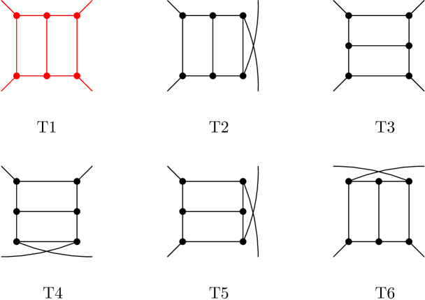
Figure 2: The reduction of the number of graphs at the topology level and the level of generic Feynman diagrams at the example of the double-box topology. For this particular example, diagrams with internal vector bosons are not shown. Topologies/diagrams in black are taken into account by applying symmetry factors onto the appropriate red diagrams rather than being computed explicitly (i.e. 3 instead of 24 generic diagrams need to be computed in total).

One of the main motivations for the results derived in this work is their application to precision calculations of the effective trilinear and quartic self-couplings of the discovered Higgs boson. In this case, one only needs to compute diagrams with identical external legs, which introduces many additional symmetries between diagrams that would otherwise not have been identical (for different external particles). Such symmetries can be found by considering the permutations of internal and external fields, which is at the heart of the canonical edges algorithm described in the previous section. Since our algorithm provides a unique edge list, two diagrams are identical if their edge lists are identical. We exploit this feature to reduce both the number of topologies to consider and the number of generic diagrams to compute. To construct a minimal and complete list of Feynman diagrams to be computed, we start by generating all possible one- and two-loop topologies using FeynArts, then calculate the corresponding edge lists, and finally remove identical topologies while simultaneously increasing a symmetry factor for them. Once a minimal set of topologies is found, we use FeynArts to insert all possible generic fields of spin 0, $\nicefrac{{1}}{{2}}$, or 1 for a renormalisable QFT. The resulting list of Feynman diagrams is again reduced by comparing edge lists and introducing appropriate symmetry factors.

In the left panel of Fig.˜2, we demonstrate the reduction of topologies and diagrams for the example of the four-point double-box diagram. The topologies T1-T6 are in general different if the external states and momenta are not identical. However, for the calculation of the effective trilinear self-coupling, all external lines are the same and the computed edge lists are identical. Therefore, we only consider T1 and introduce an additional symmetry factor of 6. In the next step, we fix all external lines to exactly the same generic scalar field and populate the internal lines with generic states of all possible spin. In the right panel of Fig.˜2, we restricted the algorithm to only consider spin 0 (S) and spin $\nicefrac{{1}}{{2}}$ (F) states for demonstrative purposes as the inclusion of vectors would greatly increase the number of diagrams to draw. In this particular sub-class of diagrams, there exists merely one diagram that contains only scalar fields. We note that this (and all other) diagram(s) inherits the symmetry factor 6 from the reduction of the topologies. In addition, FeynArts’ InsertFields function generates three more diagrams containing scalars and fermions out of which two, T1 G2 N2 and T1 G3 N3, have the same edge list and are therefore identical. In total, this sub-class of diagrams contains only 3 unique graphs (coloured in red) that need to be computed compared to the original $6\times 4=24$ diagrams.

$n$	topology-level	field-level
0	$2\to 2$	$11\to 11$
1	$3\to 3$	$25\to 25$
2	$9\to 8$	$121\to 92\,(102)$
3	$40\to 13$	$936\to 229\,(291)$
4	$265\to 29$	$10496\to 698\,(928)$

Table 1: Resulting reduction of the number of generic two-loop topologies and generic two-loop Feynman diagrams using symmetry-relations described in the text. $n$ represents the number of external legs (scalars at the field level). Numbers in brackets are obtained if diagrams, which are symmetric to diagrams with all fields replaced by their anti-fields, are kept.

In Table˜1, we summarise the reduction of the number of graphs at the level of topologies and at the level of generic fields (if scalars, fermions and vectors are allowed on the internal lines) at two loops for all scalar $n=0,1,2,3,4$-point functions. While the number of vacuum, tadpole and self-energy diagrams is only slightly reduced, the presented algorithm reduces the number of three- and four-point graphs by about one order of magnitude. It is important to note that this reduction is applied before even considering a concrete model and that, due to specific coupling structures, some models (i) may involve many more diagrams to be mapped onto the generic graphs and (ii) may also introduce more internal symmetries between certain diagrams. For both reasons, the reduction of the number of diagrams is not only a crucial step to be done before performing the tensor reduction using TwoCalc and the integral reduction discussed in Section˜2.4, but also afterwards for a given set of Feynman diagrams generated by e.g. FeynArts for a concrete model, cf. ˜3.

2.4 Integral reduction

All amplitudes are evaluated for zero external momentum. In this approximation, all scalar loop integrals can be written in the form of a $T$ or a $Y$ integral. Following the notation of Weiglein:1993hd,Goodsell:2019zfs, these are defined via

$$T_{i_{1}\cdots i_{n}} =\int\frac{\mathrm{d}^{d}q_{1}\,\mathrm{d}^{d}q_{2}}{\left[i\,\pi^{2}\left(2\,\pi\,\mu\right)^{d-4}\right]^{2}}\,\frac{1}{\left(k_{i_{1}}^{2}-m_{i_{1}}^{2}\right)\cdots\left(k_{i_{n}}^{2}-m_{i_{n}}^{2}\right)}\,,$$ (2)

$$Y_{i_{1}\cdots i_{n}}^{j_{1}\cdots j_{o}}{} =\int\frac{\mathrm{d}^{d}q_{1}\,\mathrm{d}^{d}q_{2}}{\left[i\,\pi^{2}\left(2\,\pi\,\mu\right)^{d-4}\right]^{2}}\,\frac{k_{j_{1}}^{2}\cdots k_{j_{o}}^{2}}{\left(k_{i_{1}}^{2}-m_{i_{1}}^{2}\right)\cdots\left(k_{i_{n}}^{2}-m_{i_{n}}^{2}\right)}\,,$$ (3)

where $i_{1},\dots,i_{n},j_{1},\dots,j_{o}\in\{1,2,3,4,5\}$. $d=4-2\epsilon$ with $\epsilon$ being the ultra-violet regulator, $q_{1}$ and $q_{2}$ are the loop momenta, and $\mu$ is the regularisation scale. The kinematic variables are given by

$$k_{1}=q_{1}\,,\quad k_{2}=q_{1}+p\,,\quad k_{3}=q_{2}-q_{1}\,,\quad k_{4}=q_{2}\,,\quad k_{5}=q_{2}+p,$$ (4)

where $p$ is the external momentum. We note, however, that for the rest of this work, the external momentum in $T$ or $Y$ integrals is always set to zero.

All $Y$ integrals can themselves be straightforwardly expressed in terms of $T$ integrals. These can in principle be reduced to the $T_{134}$ integral and (products of) one-loop integrals. This can, however, lead to issues during the numerical evaluation of the integrals.

Consider for example the loop integral $T_{113}(m_{1},m_{2},m_{3})$. If all masses are different, the integral can be reduced via

$$T_{113}(m_{1},m_{2},m_{3})=\frac{1}{m_{1}^{2}-m_{2}^{2}}A_{0}(m_{3}^{2})\left[A_{0}(m_{1}^{2})-A_{0}(m_{2}^{2})\right]\,.$$ (5)

This relation poses a challenge during numerical evaluation if $m_{1}\to m_{2}$. If both masses are equal, the alternative reduction formula

$$T_{113}(m_{1},m_{1},m_{3})=\frac{D-2}{2m_{1}^{2}}A_{0}(m_{1}^{2})A_{0}(m_{3}^{2})$$ (6)

should be used. If instead $m_{2}\to m_{3}$, the first relation can be used without problems.

To capture all these cases, we have generated a list of all possible mass configurations (with one or more masses being zero or equal to each other). To reduce the size of this list, we sort the mass arguments for each propagator type (e.g., $T_{113}(m_{2},m_{1},m_{3})=T_{113}(m_{1},m_{2},m_{3})$). We then derived the reduction rules for all these mass configurations, using TwoCalc. After generating this list, we checked which rules actually need to be used for the reduction and, on the other hand, which cases are already covered by a more general rule without causing any numerical instability (as in the case of $m_{2}\to m_{3}$ for the example above) and can be discarded. In this way, the number of reduction rules is greatly reduced. In the end, we obtain a list of reduction rules and an associated list of mass configurations including information about which reduction rule should be applied.

This result can then be used to implement numerical evaluation routines that automatically choose the right reduction rule based on the numerical values used as inputs for the masses. This “on-the-fly” reduction allows for stable scans of parameter spaces. A similar procedure is already used e.g. in FeynHiggs [81, 82, 83, 84, 85, 86, 87, 88, 89].

To facilitate the application of our results, we have developed the new Python package Tintegrals, which is available at

https://gitlab.com/anybsm/tint

or via “pip install Tintegrals}’’. This package provides numerical routines to evaluate all the $T$ integrals appearing in our calculation using the on-the-fly reduction explained above. Further details can be found in \crefapp:Tint.

2.5 Structure of the generic results

The steps discussed in Sections˜2.12.22.32.4 are performed for a general renormalisable theory and therefore only need to be performed once. We provide the results in the Wolfram Language format structured as follows

⬇

{

{

{1, 1, 1},

{

edge[iv[1], v[5], S[i3]], edge[iv[2], v[6], S[i4]],

edge[iv[3], v[7], S[i1]], edge[iv[4], v[8], S[i2]],

edge[v[5], v[6], -S[i9]], edge[v[5], v[7], -S[i6]],

edge[v[5], v[8], -S[i8]], edge[v[6], v[7], -S[i5]],

edge[v[6], v[8], -S[i7]]

},

-((lfac^2*SSS[i1, -i5, -i6, 1]*SSS[i2, -i7, -i8, 1]*

SSSS[i3, i6, i8, i9, 1]*SSSS[i4, i5, i7, -i9, 1]*

T[Df[k1, MS[i7]]*Df[k1, MS[i8]]*Df[k3, MS[i5]]*

Df[k3, MS[i6]]*Df[k4, MS[i9]]]

)/SF[1, 1/6, 1])

},

…

}

where the first entry is the diagram identifier used by FeynArts, the second entry is the unique edge list and the third entry is the result for the generic diagram. Therein, SF represents the various symmetry-factors assigned by FeynArts, by the reductions of the topologies, and by the reduction of diagrams discussed in Section˜2.3. For evaluations in concrete models, the replacement SF->Times should be applied. The scalar integrals

$$\texttt{T[Df[k1, m1]*...*Df[kn, mn]]}\equiv T_{i_{1}\dots i_{n}}$$ (7)

are defined in Section˜2.4 and lfac=(4*Pi)^(-2) is the loop factor. The generic couplings (here SSS[] and SSSS[] for scalar triple and quartic couplings, respectively) are defined in Goodsell:2019zfs. For a given set of diagrams in a given model, one needs to compute the edge list of every diagram, extract the couplings and masses of the diagram and insert them into the appropriate generic result above. This is discussed in the next section. For instance, the example shown above corresponds to the generic scalar double-box diagram shown in the lower right of Fig.˜2 (denoted T1 G4 N4). The full lists containing all diagrams counted in Table˜1 can be downloaded at

https://gitlab.com/anybsm/generic_scalar_2l_amplitudes.

3 Mapping to FeynArts output

To apply our generic results to a specific model, a non-trivial mapping of this model onto the conventions of our generic expressions must be performed. First, all diagrams appearing in the specific model have to be identified, and then the couplings and masses of the specific model have to be mapped to their generic counterparts. While these steps are straightforward when handling a single or a few diagrams, they can quickly become cumbersome if a larger number of diagrams is involved. We automatise these steps by providing routines to directly map FeynArts output onto our generic results. This mapping consists of the following steps:

• Use FeynArts routines to generate the Feynman diagrams.

• Map these diagrams to the canonical-form diagrams used for our generic results (applying the canonicaledges algorithm, see Section˜2.2).

• Identify the contributing fields.

• Extract the couplings that appear in the diagrams and map them to the generic couplings appearing in our generic results.

• Write out the generic results with the generic couplings and masses replaced by the model-specific expressions.

These steps can be executed with a single command. In this way, analytic results for $n=0,1,2,3,4$-point functions can be derived with minimal user intervention. An exemplary implementation of this mapping can be found at

https://gitlab.com/anybsm/generic_scalar_2l_amplitudes.

4 Cross-checks

In this Section, we cross-check our generic results by using them to derive a series of known two-loop results from the literature. Throughout the following sections, we denote the scalar $m$-point function, computed for the external fields $s_{1},\dots,s_{m}$ at the $n$-loop order, as $\Gamma_{s_{1}\dots s_{m}}^{(n)}(p_{1}^{2},\dots,p_{m}^{2})$. The superscripts “gen.” and “subloop” refer to the genuine two-loop diagrams and to the two-loop subloop renormalisation contributions, i.e. one-loop diagrams with one-loop counterterm insertions, respectively. The $n$-loop counterterm for a parameter $X$ is denoted by $\delta^{(n)}_{\rm CT}X$, while $n$-loop shifts to couplings $\lambda_{s_{1}\dots s_{m}}$ are denoted by $\delta^{(n)}\lambda_{s_{1}\dots s_{m}}$. Finally, we denote fully-renormalised loop-level quantities including external-leg corrections with a hat — e.g. $\hat{\lambda}_{hhh}$ for the complete result for the trilinear Higgs coupling.

4.1 Cross-checks in the Standard Model

As a first verification of our results in the setting of a concrete model, we reproduce in this Section the leading $\mathcal{O}(\alpha_{s}\alpha_{t})$ and $\mathcal{O}(\alpha_{t}^{2})$ corrections to $\lambda_{hhh}$ and $\lambda_{hhhh}$ in the SM, which were derived in Refs. [43, 44, 42]. We start by generating the genuine two-loop diagrams contributing at these orders to the one-, two-, three-, and four-point functions with external Higgs bosons using FeynArts and its in-built SM model file with QCD extension. At the level of the FeynArts output, we obtain for the scalar three-point (four-point) function 12 (60) diagrams at $\mathcal{O}(\alpha_{s}\alpha_{t})$ and 39 (204) at $\mathcal{O}(\alpha_{t}^{2})$; after our reduction algorithm is applied, these numbers are reduced to 4 (6) at $\mathcal{O}(\alpha_{s}\alpha_{t})$ and 13 (26) at $\mathcal{O}(\alpha_{t}^{2})$. Applying then our routines to map our generic results to these diagrams, we obtain at $\mathcal{O}(\alpha_{s}\alpha_{t})$

$$\Gamma^{(2)}_{h}\big{|}^{\text{gen.}}_{\mathcal{O}(\alpha_{s}\alpha_{t})} =\frac{\alpha_{s}m_{t}^{4}}{\pi^{3}v}\bigg{[}-\frac{3}{2\epsilon^{2}}+\frac{3\,\overline{\ln}m_{t}^{2}-2}{\epsilon}-4-\frac{\pi^{2}}{4}+4\,\overline{\ln}m_{t}^{2}-3\,\overline{\ln}^{2}m_{t}^{2}\bigg{]}\,,$$

$$\Gamma^{(2)}_{hh}(p^{2}=0)\big{|}^{\text{gen.}}_{\mathcal{O}(\alpha_{s}\alpha_{t})} =\frac{\alpha_{s}m_{t}^{4}}{\pi^{3}v^{2}}\bigg{[}-\frac{9}{2\epsilon^{2}}+\frac{9\,\overline{\ln}m_{t}^{2}}{\epsilon}-4-\frac{3\pi^{2}}{4}-9\,\overline{\ln}^{2}m_{t}^{2}\bigg{]}\,,$$

$$\Gamma^{(2)}_{hhh}(0,0,0)\big{|}^{\text{gen.}}_{\mathcal{O}(\alpha_{s}\alpha_{t})} =\frac{\alpha_{s}m_{t}^{4}}{\pi^{3}v^{3}}\bigg{[}-\frac{9}{\epsilon^{2}}+\frac{18}{\epsilon}(1+\overline{\ln}m_{t}^{2})-8-\frac{3\pi^{2}}{2}-18\,\overline{\ln}m_{t}^{2}(2+\overline{\ln}m_{t}^{2})\bigg{]}\,,$$

$$\Gamma^{(2)}_{hhhh}(0,0,0,0)\big{|}^{\text{gen.}}_{\mathcal{O}(\alpha_{s}\alpha_{t})} =\frac{\alpha_{s}m_{t}^{4}}{\pi^{3}v^{4}}\bigg{[}-\frac{9}{\epsilon^{2}}+\frac{18}{\epsilon}(3+\overline{\ln}m_{t}^{2})-80-\frac{3\pi^{2}}{2}-108\,\overline{\ln}m_{t}^{2}-18\,\overline{\ln}^{2}m_{t}^{2}\bigg{]}\,,$$ (8)

while at $\mathcal{O}(\alpha_{t}^{2})$ we have

$$\Gamma^{(2)}_{h}\big{|}^{\text{gen.}}_{\mathcal{O}(\alpha_{t}^{2})} =\ \frac{3m_{t}^{6}}{16\pi^{4}v^{3}}\bigg{[}\frac{3}{4\epsilon^{2}}+\frac{1}{\epsilon}\bigg{(}2-\frac{3}{2}\,\overline{\ln}m_{t}^{2}\bigg{)}+\frac{9}{2}+\frac{5\pi^{2}}{24}-4\,\overline{\ln}m_{t}^{2}+\frac{3}{2}\,\overline{\ln}^{2}m_{t}^{2}\bigg{]}\,,$$

$$\Gamma^{(2)}_{hh}(p^{2}=0)\big{|}^{\text{gen.}}_{\mathcal{O}(\alpha_{t}^{2})} =\ \frac{3m_{t}^{6}}{16\pi^{4}v^{4}}\bigg{[}\frac{9}{4\epsilon^{2}}+\frac{3}{\epsilon}\bigg{(}1-\frac{3}{2}\,\overline{\ln}m_{t}^{2}\bigg{)}+\frac{11}{2}+\frac{5\pi^{2}}{8}-6\,\overline{\ln}m_{t}^{2}+\frac{9}{2}\,\overline{\ln}^{2}m_{t}^{2}\bigg{]}\,,$$

$$\Gamma^{(2)}_{hhh}(0,0,0)\big{|}^{\text{gen.}}_{\mathcal{O}(\alpha_{t}^{2})} =\ \frac{3m_{t}^{6}}{16\pi^{4}v^{5}}\bigg{[}\frac{9}{2\epsilon^{2}}-\frac{3}{\epsilon}\bigg{(}1+3\,\overline{\ln}m_{t}^{2}\bigg{)}-1+\frac{5\pi^{2}}{4}+6\,\overline{\ln}m_{t}^{2}+9\,\overline{\ln}^{2}m_{t}^{2}\bigg{]}\,,$$

$$\Gamma^{(2)}_{hhhh}(0,0,0,0)\big{|}^{\text{gen.}}_{\mathcal{O}(\alpha_{t}^{2})} =\ \frac{3m_{t}^{6}}{16\pi^{4}v^{6}}\bigg{[}\frac{9}{2\epsilon^{2}}-\frac{3}{\epsilon}\bigg{(}7+3\,\overline{\ln}m_{t}^{2}\bigg{)}+11+\frac{5\pi^{2}}{4}+42\,\overline{\ln}m_{t}^{2}+9\,\overline{\ln}^{2}m_{t}^{2}\bigg{]}\,.$$ (9)

In the above equations, we use the shorthand notation $\overline{\ln}x\equiv\ln x/Q^{2}$, where $Q$ is the renormalisation scale. To these expressions, we must add contributions from subloop renormalisation, which in general form read

$$\Gamma^{(2)}_{h}\big{|}^{\text{subloop}} =\ \frac{3m_{t}^{2}}{8\pi^{2}v}\bigg{[}\frac{\delta^{(1)}_{\text{CT}}v^{2}}{v^{2}}-\delta^{(1)}_{\text{CT}}Z_{h}\bigg{]}\mathbf{A}_{0}(m_{t}^{2})$$

$$\quad-\frac{3m_{t}\delta^{(1)}_{\text{CT}}m_{t}}{2\pi^{2}v}\Big{[}\mathbf{A}_{0}(m_{t}^{2})+m_{t}^{2}\mathbf{B}_{0}(0,m_{t}^{2},m_{t}^{2})\Big{]}\,,$$

$$\Gamma^{(2)}_{hh}(p^{2}=0)\big{|}^{\text{subloop}} =\ \frac{3m_{t}^{2}}{4\pi^{2}v^{2}}\bigg{[}\frac{\delta^{(1)}_{\text{CT}}v^{2}}{v^{2}}-\delta^{(1)}_{\text{CT}}Z_{h}\bigg{]}\Big{[}\mathbf{A}_{0}(m_{t}^{2})+2m_{t}^{2}\mathbf{B}_{0}(0,m_{t}^{2},m_{t}^{2})\Big{]}$$

$$\quad-\frac{3m_{t}\delta^{(1)}_{\text{CT}}m_{t}}{2\pi^{2}v^{2}}\bigg{[}\mathbf{A}_{0}(m_{t}^{2})+m_{t}^{2}\Big{(}5\mathbf{B}_{0}(0,m_{t}^{2},m_{t}^{2})+4m_{t}^{2}\mathbf{C}_{0}(m_{t}^{2},m_{t}^{2},m_{t}^{2})\Big{)}\bigg{]}\,,$$

$$\Gamma^{(2)}_{hhh}(0,0,0)\big{|}^{\text{subloop}} =\ \frac{9m_{t}^{4}}{4\pi^{2}v^{3}}\bigg{[}\frac{\delta^{(1)}_{\text{CT}}v^{2}}{v^{2}}-\delta^{(1)}_{\text{CT}}Z_{h}\bigg{]}\Big{[}3\mathbf{B}_{0}(0,m_{t}^{2},m_{t}^{2})+4m_{t}^{2}\mathbf{C}_{0}(m_{t}^{2},m_{t}^{2},m_{t}^{2})\Big{]}$$

$$\quad-\frac{18m_{t}^{3}\delta^{(1)}_{\text{CT}}m_{t}}{\pi^{2}v^{3}}\bigg{[}\mathbf{B}_{0}(0,m_{t}^{2},m_{t}^{2})+m_{t}^{2}\Big{(}3\mathbf{C}_{0}(m_{t}^{2},m_{t}^{2},m_{t}^{2})$$

$$\hskip 113.81102pt+2m_{t}^{2}\mathbf{D}_{0}(m_{t}^{2},m_{t}^{2},m_{t}^{2},m_{t}^{2})\Big{)}\bigg{]}\,,$$

$$\Gamma^{(2)}_{hhhh}(0,0,0,0)\big{|}^{\text{subloop}} =\ \frac{9m_{t}^{4}}{\pi^{2}v^{4}}\bigg{[}\frac{\delta^{(1)}_{\text{CT}}v^{2}}{v^{2}}-\delta^{(1)}_{\text{CT}}Z_{h}\bigg{]}$$

$$\qquad\times\bigg{[}\mathbf{B}_{0}(0,m_{t}^{2},m_{t}^{2})+8m_{t}^{2}\Big{(}\mathbf{C}_{0}(m_{t}^{2},m_{t}^{2},m_{t}^{2})+m_{t}^{2}\mathbf{D}_{0}(m_{t}^{2},m_{t}^{2},m_{t}^{2},m_{t}^{2})\Big{)}\bigg{]}$$

$$\quad-\frac{18m_{t}^{3}\delta^{(1)}_{\text{CT}}m_{t}}{\pi^{2}v^{4}}\times\bigg{\{}\mathbf{B}_{0}(0,m_{t}^{2},m_{t}^{2})+m_{t}^{2}\bigg{[}13\mathbf{C}_{0}(m_{t}^{2},m_{t}^{2},m_{t}^{2})$$

$$\hskip 113.81102pt+4m_{t}^{2}\Big{(}7\mathbf{D}_{0}(m_{t}^{2},m_{t}^{2},m_{t}^{2},m_{t}^{2})$$

$$\hskip 113.81102pt+4m_{t}^{2}\mathbf{E}_{0}(m_{t}^{2},m_{t}^{2},m_{t}^{2},m_{t}^{2},m_{t}^{2})\Big{)}\bigg{]}\bigg{\}}\,,$$

where $\mathbf{A}_{0}$, $\mathbf{B}_{0}$, $\mathbf{C}_{0}$, $\mathbf{D}_{0}$, $\mathbf{E}_{0}$ denote standard, unrenormalised, one-loop Passarino-Veltmann functions [90], and where we have omitted momenta arguments for $\mathbf{C}_{0}$, $\mathbf{D}_{0}$, and $\mathbf{E}_{0}$ as these are all set to zero. We obtain the different counterterms by using the functionalities of FormCalc [91, 92] and the default SM model file for FeynArts. Moreover, for the present calculation, we only need contributions of $\mathcal{O}(\alpha_{s})$ (for $\delta^{(1)}_{\text{CT}}m_{t}$ only) and of $\mathcal{O}(\alpha_{t})$. The particular cases of the Passarino-Veltmann functions in the above equation can be simplified using the relations

$$\mathbf{C}_{0}(x,x,x)=\ \frac{1}{2}\frac{\partial}{\partial x}\mathbf{B}_{0}(0,x,x)\,,\quad \mathbf{D}_{0}(x,x,x,x)=\ \frac{1}{6}\frac{\partial^{2}}{\partial x^{2}}\mathbf{B}_{0}(0,x,x)\,,$$

$$\mathbf{E}_{0}(x,x,x,x,x)= \ \frac{1}{24}\frac{\partial^{3}}{\partial x^{3}}\mathbf{B}_{0}(0,x,x)\,.$$ (10)

$\overline{\text{MS}}$ renormalisation:

Starting with an $\overline{\text{MS}}$ renormalisation scheme, we have

$$\frac{1}{m_{t}}\delta^{(1)}_{\text{CT}}m_{t}^{\overline{\text{MS}}} =\frac{1}{\epsilon}\bigg{[}-\frac{\alpha_{s}}{\pi}+\frac{3m_{t}^{2}}{32\pi^{2}v^{2}}\bigg{]}\,,$$

$$\delta^{(1)}_{\text{CT}}Z_{h}^{\overline{\text{MS}}}=\left(\frac{\delta^{(1)}_{\text{CT}}v^{2}}{v^{2}}\right)^{\overline{\text{MS}}} =-\frac{3m_{t}^{2}}{8\pi^{2}v^{2}\epsilon}\,.$$ (11)

Additionally, genuine two-loop counterterms for $\lambda_{hhh}$ and $\lambda_{hhhh}$ are also required. However, in the SM (as well as in aligned BSM models) it can be shown that such a pure two-loop counterterm is fixed entirely in terms of the two-loop tadpole and mass counterterms — adapting for instance the discussion in Ref. [27] to the two-loop order. It follows that the combinations

$$\Gamma^{(2)}_{hhh}(0,0,0)\big{|}^{\text{gen.}}+\Gamma^{(2)}_{hhh}(0,0,0)\big{|}^{\text{subloop}}$$

$$-\frac{3}{v}\bigg{[}\Gamma^{(2)}_{hh}(0)\big{|}^{\text{gen.}}+\Gamma^{(2)}_{hh}(0)\big{|}^{\text{subloop}}-\frac{1}{v}\bigg{(}\Gamma^{(2)}_{h}\big{|}^{\text{gen.}}+\Gamma^{(2)}_{h}\big{|}^{\text{subloop}}\bigg{)}\bigg{]}$$ (12)

and

$$\Gamma^{(2)}_{hhhh}(0,0,0,0)\big{|}^{\text{gen.}}+\Gamma^{(2)}_{hhhh}(0,0,0,0)\big{|}^{\text{subloop}}$$

$$-\frac{3}{v^{2}}\bigg{[}\Gamma^{(2)}_{hh}(0)\big{|}^{\text{gen.}}+\Gamma^{(2)}_{hh}(0)\big{|}^{\text{subloop}}-\frac{1}{v}\bigg{(}\Gamma^{(2)}_{h}\big{|}^{\text{gen.}}+\Gamma^{(2)}_{h}\big{|}^{\text{subloop}}\bigg{)}\bigg{]}$$ (13)

are UV-finite, and correspond to the Higgs mass and tadpole being renormalised on-shell. These two expressions — including the finite parts of the one- and two-point functions — can then be identified, up to a minus sign, with the two-loop corrections to the trilinear and quartic Higgs couplings (i.e. $-\delta^{(2)}\lambda_{hhh}$ and $-\delta^{(2)}\lambda_{hhhh}$), respectively. Combining all expressions above, we then find

$$\left.\delta^{(2)}\lambda_{hhh}\right|^{\overline{\text{MS}}}= \ \frac{2\alpha_{s}m_{t}^{4}}{\pi^{3}v^{3}}\big{[}1+6\overline{\ln}m_{t}^{2}\big{]}-\frac{3m_{t}^{6}}{16\pi^{4}v^{5}}\big{[}6\overline{\ln}m_{t}^{2}-7\big{]}\,,$$

$$\left.\delta^{(2)}\lambda_{hhhh}\right|^{\overline{\text{MS}}}= \ \frac{16\alpha_{s}m_{t}^{4}}{\pi^{3}v^{4}}\big{[}2+3\overline{\ln}m_{t}^{2}\big{]}-\frac{3m_{t}^{6}}{2\pi^{4}v^{6}}\big{[}3\overline{\ln}m_{t}^{2}-2\big{]}\,,$$ (14)

in terms of $\overline{\text{MS}}$-renormalised parameters $m_{t}$ and $v$, and with the Higgs wave-function renormalisation (WFR) $\overline{\text{MS}}$ as well. These results correspond exactly to Eqs. (V.2) and (V.3) in Braathen:2019zoh.

On-shell renormalisation:

Next, one can also consider a full on-shell (OS) renormalisation scheme. The OS-scheme counterterms of the top-quark mass and the Higgs WFR can be found to be, up to $\mathcal{O}(\epsilon^{0})$,

$$\frac{1}{m_{t}}\delta^{(1)}_{\text{CT}}m_{t}^{\text{OS}}= \ \frac{\alpha_{s}}{\pi}\bigg{[}-\frac{1}{\epsilon}+\overline{\ln}m_{t}^{2}-\frac{4}{3}\bigg{]}+\frac{3m_{t}^{2}}{32\pi^{2}v^{2}}\bigg{[}\frac{1}{\epsilon}+\frac{8}{3}-\overline{\ln}m_{t}^{2}\bigg{]}\,,$$

$$\delta^{(1)}_{\text{CT}}Z_{h}^{\text{OS}}= \ \frac{3m_{t}^{2}}{8\pi^{2}v^{2}}\bigg{[}-\frac{1}{\epsilon}+\frac{2}{3}+\overline{\ln}m_{t}^{2}\bigg{]}\,.$$ (15)

Depending on the choice of input scheme for electroweak parameters, the finite part of the corresponding counterterm of the EW vacuum expectation value (VEV) takes different forms. A first choice (following Ref. [43, 44]) is to relate $v$ to the Fermi constant $G_{F}$, which results in

$$\left(\frac{\delta^{(1)}_{\text{CT}}v^{2}}{v^{2}}\right)^{\text{OS, }G_{F}} =\frac{3m_{t}^{2}}{16\pi^{2}v^{2}}\bigg{[}-\frac{2}{\epsilon}+2\overline{\ln}m_{t}^{2}-1\bigg{]}\,.$$ (16)

Another possibility is instead to relate the EW VEV to $M_{W}$, $M_{Z}$, and the electric charge $e$, and in this case, the OS counterterm for $v$ reads

$$\left(\frac{\delta^{(1)}_{\text{CT}}v^{2}}{v^{2}}\right)^{\text{OS, }\alpha_{\text{em}}} =\frac{\delta^{(1)}_{\text{CT}}(M_{W}^{2})^{\text{OS}}}{M_{W}^{2}}+\frac{c_{W}^{2}}{s_{W}^{2}}\bigg{(}\frac{\delta^{(1)}_{\text{CT}}(M_{Z}^{2})^{\text{OS}}}{M_{Z}^{2}}-\frac{\delta^{(1)}_{\text{CT}}(M_{W}^{2})^{\text{OS}}}{M_{W}^{2}}\bigg{)}-\frac{2\delta^{(1)}_{\text{CT}}e^{\text{OS}}}{e}=$$

$$=\frac{3m_{t}^{2}}{16\pi^{2}v^{2}}\bigg{[}-\frac{2}{\epsilon}+2\overline{\ln}m_{t}^{2}-1-\frac{c_{W}^{2}}{s_{W}^{2}}\bigg{]}\,.$$ (17)

With the first choice, we find

$$\left.\delta^{(2)}\lambda_{hhh}\right|^{\text{OS},\ G_{F}}= \ \frac{18\,\alpha_{s}M_{t}^{4}}{\pi^{3}v_{\text{OS}}^{3}}-\frac{117M_{t}^{6}}{32\pi^{4}v_{\text{OS}}^{5}}\,,$$

$$\left.\delta^{(2)}\lambda_{hhhh}\right|^{\text{OS},\ G_{F}}= \ \frac{96\,\alpha_{s}M_{t}^{4}}{\pi^{3}v_{\text{OS}}^{4}}-\frac{39M_{t}^{6}}{2\pi^{4}v_{\text{OS}}^{6}}\,,$$ (18)

in terms of the top-quark pole mass $M_{t}$ and of $v_{\text{OS}}\equiv(\sqrt{2}G_{F})^{-1/2}\simeq 246.22$ GeV. These expressions agree exactly with those in Eq. (V.6) of Braathen:2019zoh. In the second case, we obtain the following new results

$$\left.\delta^{(2)}\lambda_{hhh}\right|^{\text{OS},\ \alpha_{\text{em}}}= \ \frac{18\,\alpha_{s}M_{t}^{4}}{\pi^{3}\bar{v}_{\text{OS}}^{3}}-\frac{M_{t}^{6}}{32\pi^{4}\bar{v}_{\text{OS}}^{5}}\left[117+\frac{27\,c_{W}^{2}}{s_{W}^{2}}\right]\,,$$

$$\left.\delta^{(2)}\lambda_{hhhh}\right|^{\text{OS},\ \alpha_{\text{em}}}= \ \frac{96\,\alpha_{s}M_{t}^{4}}{\pi^{3}\bar{v}_{\text{OS}}^{4}}-\frac{M_{t}^{6}}{2\pi^{4}\bar{v}_{\text{OS}}^{6}}\left[39+\frac{9\,c_{W}^{2}}{s_{W}^{2}}\right]\,,$$ (19)

where the same top-quark pole mass $M_{t}$ is employed but with $\bar{v}_{\text{OS}}\equiv\frac{2M_{W}s_{W}}{e}\simeq 250.19$ GeV as well as $e\equiv\sqrt{4\pi\alpha_{\text{em}}(0)}$ and $c_{W}\equiv M_{W}/M_{Z}$ is the cosine of the weak mixing angle.

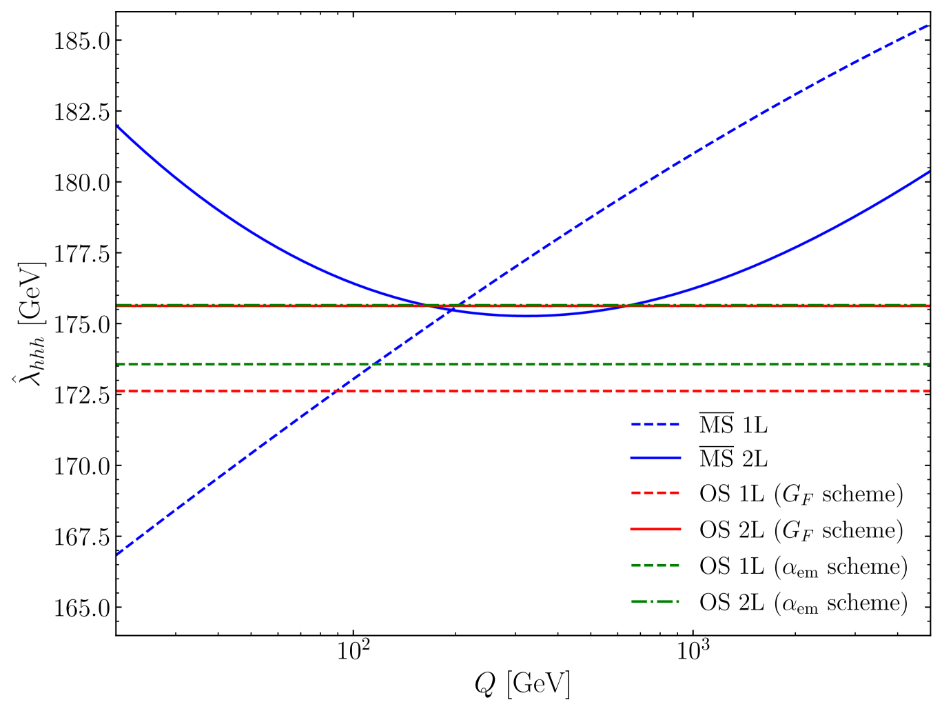
Figure 3: Trilinear Higgs coupling in the Standard Model at leading one- and two-loop orders. Blue curves correspond to the $\overline{\text{MS}}$ scheme, while the red and green ones correspond to two versions of OS scheme, with the EW VEV related respectively to $G_{F}$ (red) and to $M_{W}$, $M_{Z}$ and $\alpha_{\text{em}}(0)$ (green).

These results are illustrated in ˜3, which compares results for the total loop-corrected predictions for $\hat{\lambda}_{hhh}$ at leading one- (dashed lines) and two-loop (solid or dot-dashed lines) orders (we note that, following the choice made in Braathen:2019zoh,Braathen:2019pxr, we do not include external-leg corrections in the $\overline{\text{MS}}$ results for $\hat{\lambda}_{hhh}$). Results in the three renormalisation schemes discussed above — $\overline{\text{MS}}$, OS with the EW VEV related to $G_{F}$, and OS with the EW VEV related to $M_{W}$, $M_{Z}$ and $\alpha_{\text{em}}(0)$ — are indicated by the blue, red, and green colours, respectively. As expected, both versions of OS schemes are manifestly independent of the renormalisation scale. At one loop, the predictions for $\hat{\lambda}_{hhh}$ in the two OS schemes differ by about $950$ MeV, while at two loops this difference is reduced to $23$ MeV — which can be used as an estimate of three-loop mixed QCD–EW corrections, which are not included in this calculation.

4.2 Cross-checks in the $\mathbb{Z}_{2}$-symmetric singlet extension of the SM

As a first example of a BSM model, we investigate in this Section the application of our generic results in the context of the $\mathbb{Z}_{2}$-symmetric singlet extension of the SM ($\mathbb{Z}_{2}$SSM).

4.2.1 The model

The scalar sector of the $\mathbb{Z}_{2}$SSM contains the usual SM-like doublet $\Phi$, decomposed as

$$\Phi=\frac{1}{\sqrt{2}}\begin{pmatrix}\sqrt{2}G^{+}\\ v+h+iG\end{pmatrix}\,,$$ (20)

and a singlet $S$ that is charged under an unbroken global $\mathbb{Z}_{2}$ symmetry. In terms of these two states, the tree-level scalar potential of the $\mathbb{Z}_{2}$SSM can be written as

$$V_{\mathbb{Z}_{2}}(\Phi,S)=\mu^{2}|\Phi|^{2}+\frac{\lambda_{H}}{2}|\Phi|^{4}+\frac{\mu_{S}^{2}}{2}S^{2}+\frac{\lambda_{S}}{2}S^{4}+\frac{\lambda_{SH}}{2}S^{2}|\Phi|^{2}\,.$$ (21)

The minimisation condition of the tree-level potential reads

$$0=\frac{1}{v}\frac{\partial V_{\mathbb{Z}_{2}}}{\partial h}\bigg{|}_{h=0}=\frac{t_{h}^{(0)}}{v}=\mu^{2}+\frac{1}{2}\lambda_{H}v^{2}\,,$$ (22)

while the tree-level mass eigenstates are

$$m_{h}^{2}=\mu^{2}+\frac{3}{2}\lambda_{H}v^{2}\,,\quad\text{and}\quad m_{S}^{2}=\mu_{S}^{2}+\frac{1}{2}\lambda_{SH}v^{2}\,.$$ (23)

These relations allow us to rewrite, at the tree level, the quartic couplings $\lambda_{H}$ and $\lambda_{SH}$ as

$$\lambda_{H}=\frac{m_{h}^{2}}{v^{2}}-\frac{t_{h}^{(0)}}{v^{3}}\,,\quad\text{and}\quad\lambda_{SH}=\frac{2(m_{S}^{2}-\mu_{S}^{2})}{v^{2}}\,.$$ (24)

We consider the limit $m_{S}\gg m_{h}$ such that $m_{h}\approx 0$ and consequently $\lambda_{H}\approx 0$ are good approximations beyond tree-level. We turn now to the discussion of the counterterms required, in this approximation, to obtain a UV-finite result for $\lambda_{hhh}$ at two loops, expressed entirely in terms of OS quantities. First, for the subloop renormalisation we require the following conditions and counterterms:

• an OS renormalisation of the tree-level masses and the scalar fields:

  $$\delta^{(1)}_{\text{CT}}m_{h}^{2}=\Sigma^{(1)}_{hh}(p^{2}=0)\,,\quad\text{and}\quad\delta^{(1)}_{\text{CT}}m_{S}^{2}=\Sigma^{(1)}_{SS}(p^{2}=m_{S}^{2})\,,$$ (25)

  and

  $$\delta^{(1)}_{\text{CT}}Z_{h}=-\left.\frac{\partial}{\partial p^{2}}\Sigma^{(1)}_{hh}(p^{2})\right|_{p^{2}=0}\,,\quad\text{and}\quad\delta^{(1)}_{\text{CT}}Z_{S}=-\left.\frac{\partial}{\partial p^{2}}\Sigma^{(1)}_{SS}(p^{2})\right|_{p^{2}=m_{S}^{2}}\,,$$ (26)

• an OS renormalisation of the tadpole $\hat{t}_{h}$:

  $$\hat{t}_{h}=t_{h}^{(0)}+t_{h}^{(1)}+\delta^{(1)}_{\text{CT}}t_{h}=0\Rightarrow\delta^{(1)}_{\text{CT}}t_{h}=-t_{h}^{(1)},\,$$ (27)

  and finally,

• an “OS-like” (or “decoupling inspired”) renormalisation of $\mu_{S}$, demanding the correct decoupling behaviour of corrections involving the singlet self-coupling, following Braathen:2019zoh:

  $$\delta^{(1)}_{\text{CT}}\mu_{S}^{2}=\frac{3\lambda_{S}\mu_{S}^{2}}{8\pi^{2}m_{S}^{2}}\textbf{A}_{0}(m_{S}^{2})$$ (28)

  where $\textbf{A}_{0}$ is the (unrenormalised) scalar one-loop one-point function [90].

To cancel all divergences at the two-loop level and to ensure a proper OS description, we employ the following two-loop counterterms:

• mass counterterm of the SM-like Higgs boson:

  $$\delta^{(2)}_{\text{CT}}m_{h}^{2}=\Sigma^{(2)}_{hh}(p^{2}=0)+\frac{1}{2}\delta^{(1)}_{\text{CT}}Z_{hh}\delta^{(1)}_{\text{CT}}m_{h}^{2}\,,$$ (29)

• two-loop tadpole:

  $$\delta^{(2)}_{\text{CT}}t_{h}=-t_{h}^{(2)}-\delta^{(1)}_{\text{CT}}Z_{hh}\delta^{(1)}_{\text{CT}}t_{h}\,.$$ (30)

With these ingredients, we can construct the renormalised trilinear coupling at one loop

$$\delta^{(1)}\lambda_{hhh}=\delta^{(1)}_{\text{diag.}}\lambda_{hhh}+\frac{3}{v^{2}}\left(\delta^{(1)}_{\text{CT}}t_{h}-v\,\delta^{(1)}_{\text{CT}}m_{h}^{2}\right)\,,$$ (31)

and at two loops

$$\delta^{(2)}\lambda_{hhh}=\frac{3}{2}\delta^{(1)}\lambda_{hhh}\left(\delta^{(1)}_{\text{CT}}Z_{hh}+\Sigma_{hh}^{\prime}(0)\right)+\delta^{(2)}_{\text{diag.}}\lambda_{hhh}+\frac{3}{v^{2}}\left(\delta^{(2)}_{\text{CT}}t_{h}-v\,\delta^{(2)}_{\text{CT}}m_{h}^{2}\right)\,,$$ (32)

where the subscript “diag” denotes the sum of all Feynman-diagrammatic contributions, including one-loop diagrams with one-loop mass- and vertex-counterterm insertions (that stem from the subloop renormalisation). In ˜32 we introduce the notation $\Sigma^{\prime}(x)=\frac{\partial}{\partial p^{2}}\Sigma(p^{2})\big{|}_{p^{2}=x}$.

4.2.2 Leading two-loop corrections to the trilinear Higgs coupling

The renormalisation procedure described in the previous paragraph combined with the diagrammatic calculation of all one- and two-loop diagrams contributing to one-, two- and three-point functions of the Higgs boson using the generic results from Sections˜23 leads to exact agreement with the results obtained for the leading BSM contributions to $\lambda_{hhh}$ in the $\mathbb{Z}_{2}$SSM in Braathen:2019zoh. In contrast to our results, in Braathen:2019zoh the corrections to the trilinear coupling were obtained by taking field-derivatives of the one- and two-loop effective potential. Furthermore, in this reference, an $\overline{\text{MS}}$ renormalisation was performed already at the level of the effective potential; finite counterterm shifts were afterwards included at the level of the derivatives of the effective potential in order to obtain a full OS result for $\lambda_{hhh}$. Therefore, the approach presented in the present work is a strong independent cross-check of both the results in Braathen:2019zoh as well as of the generic results obtained in this work. First, we obtain for the genuine two-loop corrections to the one-, two-, and three-point functions the following expressions

$$\Gamma^{(2)}_{h}\big{|}^{\text{gen.}}_{\mathcal{O}(\lambda_{S}^{0})} =\frac{(m_{S}^{2}-\mu_{S}^{2})^{2}}{128\pi^{4}v^{3}}\bigg{[}\frac{\mu_{S}^{2}-2m_{S}^{2}}{\epsilon^{2}}+\frac{1}{\epsilon}\big{(}\mu_{S}^{2}-4m_{S}^{2}+(4m_{S}^{2}-2\mu_{S}^{2})\overline{\ln}m_{S}^{2}\big{)}$$

$$\qquad\qquad\qquad\quad+\mu_{S}^{2}\left(1+\frac{\pi^{2}}{6}\right)-2m_{S}^{2}\left(4+\frac{\pi^{2}}{6}\right)$$

$$\qquad\qquad\qquad\quad-2\overline{\ln}m_{S}^{2}\big{(}\mu_{S}^{2}-4m_{S}^{2}+(2m_{S}^{2}-\mu_{S}^{2})\overline{\ln}m_{S}^{2}\big{)}\bigg{]}\,,$$

$$\Gamma^{(2)}_{h}\big{|}^{\text{gen.}}_{\mathcal{O}(\lambda_{S})} =\frac{3\lambda_{S}m_{S}^{2}(m_{S}^{2}-\mu_{S}^{2})}{128\pi^{4}v}\bigg{[}-\frac{1}{\epsilon^{2}}+\frac{2\overline{\ln}m_{S}^{2}-1}{\epsilon}-1-\frac{\pi^{2}}{6}-2(\overline{\ln}m_{S}^{2}-1)\overline{\ln}m_{S}^{2}\bigg{]}\,,$$

$$\Gamma^{(2)}_{hh}(p^{2}=0)\big{|}^{\text{gen.}}_{\mathcal{O}(\lambda_{S}^{0})} =\frac{(m_{S}^{2}-\mu_{S}^{2})^{2}}{128\pi^{4}v^{4}}\bigg{[}\frac{5\mu_{S}^{2}-6m_{S}^{2}}{\epsilon^{2}}-\frac{1}{\epsilon}\bigg{(}4m_{S}^{2}+3\mu_{S}^{2}-\frac{4\mu_{S}^{4}}{m_{S}^{2}}-2(6m_{S}^{2}-5\mu_{S}^{2})\overline{\ln}m_{S}^{2}\bigg{)}$$

$$\hskip 71.13188pt+\frac{4\mu_{S}^{4}}{m_{S}^{2}}-2m_{S}^{2}\left(4+\frac{\pi^{2}}{2}\right)-\mu_{S}^{2}\left(3-\frac{5\pi^{2}}{6}\right)$$

$$\hskip 71.13188pt+2\overline{\ln}m_{S}^{2}\bigg{(}4m_{S}^{2}+3\mu_{S}^{2}-\frac{4\mu_{S}^{4}}{m_{S}^{2}}+(5\mu_{S}^{2}-6m_{S}^{2})\overline{\ln}m_{S}^{2}\bigg{)}\bigg{]}\,,$$

$$\Gamma^{(2)}_{hh}(p^{2}=0)\big{|}^{\text{gen.}}_{\mathcal{O}(\lambda_{S})} =\frac{3\lambda_{S}(m_{S}^{2}-\mu_{S}^{2})}{128\pi^{4}v^{2}}\bigg{[}\frac{2\mu_{S}^{2}-3m_{S}^{2}}{\epsilon^{2}}+\frac{m_{S}^{2}-2\mu_{S}^{2}+(6m_{S}^{2}-4\mu_{S}^{2})\overline{\ln}m_{S}^{2}}{\epsilon}$$

$$\hskip 88.2037pt+m_{S}^{2}\left(1-\frac{\pi^{2}}{2}\right)-2\mu_{S}^{2}\left(1-\frac{\pi^{2}}{6}\right)$$

$$\hskip 88.2037pt-2\overline{\ln}m_{S}^{2}\Big{(}m_{S}^{2}-2\mu_{S}^{2}+(3m_{S}^{2}-2\mu_{S}^{2})\overline{\ln}m_{S}^{2}\Big{)}\bigg{]}\,,$$

$$\Gamma^{(2)}_{hhh}(0,0,0)\big{|}^{\text{gen.}}_{\mathcal{O}(\lambda_{S}^{0})} =\frac{4(m_{S}^{2}-\mu_{S}^{2})^{3}}{128\pi^{4}v^{5}}\bigg{[}-\frac{3}{\epsilon^{2}}+\frac{1}{\epsilon}\bigg{(}4-\frac{5\mu_{S}^{2}}{m_{S}^{2}}-\frac{2\mu_{S}^{4}}{m_{S}^{4}}+6\overline{\ln}m_{S}^{2}\bigg{)}$$

$$\hskip 82.51282pt+\frac{3\mu_{S}^{2}}{m_{S}^{2}}-\frac{6\mu_{S}^{4}}{m_{S}^{4}}-\frac{\pi^{2}}{2}+\bigg{(}\frac{10\mu_{S}^{2}}{m_{S}^{2}}+\frac{4\mu_{S}^{4}}{m_{S}^{4}}-8\bigg{)}\overline{\ln}m_{S}^{2}-6\overline{\ln}^{2}m_{S}^{2}\bigg{]}\,,$$

$$\Gamma^{(2)}_{hhh}(0,0,0)\big{|}^{\text{gen.}}_{\mathcal{O}(\lambda_{S})} =\frac{3\lambda_{S}(m_{S}^{2}-\mu_{S}^{2})^{2}}{128\pi^{4}v^{3}}\bigg{[}-\frac{6}{\epsilon^{2}}+\frac{1}{\epsilon}\bigg{(}14-\frac{8\mu_{S}^{2}}{m_{S}^{2}}+12\overline{\ln}m_{S}^{2}\bigg{)}$$

$$\hskip 92.47145pt-2+\frac{8\mu_{S}^{2}}{m_{S}^{2}}-\pi^{2}+4\bigg{(}\frac{4\mu_{S}^{2}}{m_{S}^{2}}-7\bigg{)}\overline{\ln}m_{S}^{2}-12\overline{\ln}^{2}m_{S}^{2}\bigg{]}\,,$$ (33)

where we have separated terms involving $\lambda_{S}$ or not, in order to make the expressions more easily readable. As a further example of the impact of our algorithm to reduce the number of diagrams to calculate, we note that in the $\mathbb{Z}_{2}$SSM, the number of diagrams contributing to the leading BSM corrections to the Higgs three-point function decreases from 57 (at the Particles level) to 18 after reduction. Next, we require the subloop renormalisation contributions, which are found to be

$$\Gamma^{(2)}_{h}\big{|}^{\text{subloop}} =\frac{m_{S}^{2}-\mu_{S}^{2}}{32\pi^{2}v}\bigg{[}\bigg{(}\frac{\delta^{(1)}_{\text{CT}}v^{2}}{v^{2}}+\frac{2\delta^{(1)}_{\text{CT}}\lambda_{SH}}{\lambda_{SH}}+\delta^{(1)}_{\text{CT}}Z_{h}-2\delta^{(1)}_{\text{CT}}Z_{S}\bigg{)}\mathbf{A}_{0}(m_{S}^{2})$$

$$\hskip 71.13188pt+2\delta^{(1)}_{\text{CT}}m_{S}^{2}\,\mathbf{B}_{0}(0,m_{S}^{2},m_{S}^{2})\bigg{]}\,,$$

$$\Gamma^{(2)}_{hh}(p^{2}=0)\big{|}^{\text{subloop}} =\frac{m_{S}^{2}-\mu_{S}^{2}}{16\pi^{2}v^{2}}\Bigg{\{}\bigg{(}\frac{\delta^{(1)}_{\text{CT}}\lambda_{SH}}{\lambda_{SH}}+\delta^{(1)}_{\text{CT}}Z_{h}-\delta^{(1)}_{\text{CT}}Z_{S}\bigg{)}\mathbf{A}_{0}(m_{S}^{2})$$

$$\hskip-42.67912pt+\bigg{[}\delta^{(1)}_{\text{CT}}m_{S}^{2}+2(m_{S}^{2}-\mu_{S}^{2})\bigg{(}\frac{\delta^{(1)}_{\text{CT}}v^{2}}{v^{2}}+\frac{2\delta^{(1)}_{\text{CT}}\lambda_{SH}}{\lambda_{SH}}+\delta^{(1)}_{\text{CT}}Z_{h}-2\delta^{(1)}_{\text{CT}}Z_{S}\bigg{)}\bigg{]}\mathbf{B}_{0}(0,m_{S}^{2},m_{S}^{2})$$

$$\hskip 85.35826pt+4\delta^{(1)}_{\text{CT}}m_{S}^{2}(m_{S}^{2}-\mu_{S}^{2})\,\mathbf{C}_{0}(m_{S}^{2},m_{S}^{2},m_{S}^{2})\Bigg{\}}\,,$$

$$\Gamma^{(2)}_{hhh}(0,0,0)\big{|}^{\text{subloop}} =\frac{3(m_{S}^{2}-\mu_{S}^{2})^{2}}{16\pi^{2}v^{3}}\Bigg{\{}\bigg{(}4\frac{\delta^{(1)}_{\text{CT}}\lambda_{SH}}{\lambda_{SH}}+\frac{\delta^{(1)}_{\text{CT}}v^{2}}{v^{2}}+3\delta^{(1)}_{\text{CT}}Z_{h}-4\delta^{(1)}_{\text{CT}}Z_{S}\bigg{)}\mathbf{B}_{0}(0,m_{S}^{2},m_{S}^{2})$$

$$\hskip-71.13188pt+4\bigg{[}\delta^{(1)}_{\text{CT}}m_{S}^{2}+(m_{S}^{2}-\mu_{S}^{2})\bigg{(}\frac{2\delta^{(1)}_{\text{CT}}\lambda_{SH}}{\lambda_{SH}}+\frac{\delta^{(1)}_{\text{CT}}v^{2}}{v^{2}}+\delta^{(1)}_{\text{CT}}Z_{h}-2\delta^{(1)}_{\text{CT}}Z_{S}\bigg{)}\bigg{]}\mathbf{C}_{0}(m_{S}^{2},m_{S}^{2},m_{S}^{2})$$

$$\hskip 14.22636pt+8(m_{S}^{2}-\mu_{S}^{2})\delta^{(1)}_{\text{CT}}m_{S}^{2}\,\mathbf{D}_{0}(m_{S}^{2},m_{S}^{2},m_{S}^{2},m_{S}^{2})\Bigg{\}}\,,$$ (34)

having here again omitted vanishing momenta in the arguments of $\mathbf{C}_{0}$ and $\mathbf{D}_{0}$, as in ˜4.1. We have expressed these contributions in terms of the counterterm for the portal coupling $\lambda_{SH}$. This can be related to the counterterms presented in the previous Section by differentiating the expression in ˜24, i.e.

$$\delta^{(1)}_{\text{CT}}\lambda_{SH}=\frac{2}{v^{2}}\left(\delta^{(1)}_{\text{CT}}m_{S}^{2}-\delta^{(1)}_{\text{CT}}\mu_{S}^{2}\right)-\frac{2(m_{S}^{2}-\mu_{S}^{2})}{v^{2}}\frac{\delta^{(1)}_{\text{CT}}v^{2}}{v^{2}}\,.$$ (35)

Employing then the counterterm definitions discussed above (and keeping in mind the minus sign between the effective trilinear coupling and the three-point functions), we obtain results for $\delta^{(2)}\lambda_{hhh}$, first in terms of $\overline{\text{MS}}$-renormalised BSM parameters $m_{S}$ and $\mu_{S}$ (but with OS-renormalised Higgs mass and tadpole)

$$\delta^{(2)}\lambda_{hhh}\big{|}^{\overline{\text{MS}}}_{\mathcal{O}(\lambda_{S}^{0})}= \ \frac{m_{S}^{4}}{16\pi^{4}v^{5}}\left(1-\frac{\mu_{S}^{2}}{m_{S}^{2}}\right)^{4}\big{[}-m_{S}^{2}-2\mu_{S}^{2}+(2m_{S}^{2}+\mu_{S})\overline{\ln}m_{S}^{2}\big{]}\,,$$

$$\delta^{(2)}\lambda_{hhh}\big{|}^{\overline{\text{MS}}}_{\mathcal{O}(\lambda_{S})}= \ \frac{3\lambda_{S}m_{S}^{4}}{32\pi^{4}v^{3}}\left(1-\frac{\mu_{S}^{2}}{m_{S}^{2}}\right)^{3}\big{[}1+2\overline{\ln}m_{S}^{2}\big{]}\,,$$ (36)

where we again split the results between terms involving $\lambda_{S}$ or not to facilitate reading. Using OS counterterms, we find

$$\delta^{(2)}\lambda_{hhh}\big{|}^{\text{OS}}_{\mathcal{O}(\lambda_{S}^{0})}= \ \frac{3M_{S}^{6}}{16\pi^{4}v^{5}}\left(1-\frac{\tilde{\mu}_{S}^{2}}{M_{S}^{2}}\right)^{4}-\frac{M_{S}^{6}}{128\pi^{4}v^{5}}\left(1-\frac{\tilde{\mu}_{S}^{2}}{M_{S}^{2}}\right)^{5}+\frac{21M_{S}^{4}\,M_{t}^{2}}{128\pi^{4}v^{5}}\left(1-\frac{\tilde{\mu}_{S}^{2}}{M_{S}^{2}}\right)^{3}$$

$$+\frac{3M_{S}^{2}\,M_{t}^{4}}{32\pi^{4}v^{5}}\left(1-\frac{\tilde{\mu}_{S}^{2}}{M_{S}^{2}}\right)^{2}\,,$$

$$\delta^{(2)}\lambda_{hhh}\big{|}^{\text{OS}}_{\mathcal{O}(\lambda_{S})}= \ \frac{9\lambda_{S}M_{S}^{4}}{32\pi^{4}v^{3}}\left(1-\frac{\tilde{\mu}_{S}^{2}}{M_{S}^{2}}\right)^{3}\,,$$ (37)

where $M_{S}$ and $\tilde{\mu}_{S}$ denote the OS-renormalised BSM mass parameters, and $M_{t}$ is the (OS) top-quark mass. We recall that because $\lambda_{S}$ only enters the trilinear Higgs coupling at the two-loop order, no counterterm is needed for it. As stated at the beginning of the Section, our ˜4.2.24.2.2 reproduce exactly the results in Braathen:2019zoh (see Eqs. (V.25) and (V.31) therein).

4.2.3 Matching the $\mathbb{Z}_{2}$SSM onto the SM

Another result from the literature that we can reproduce in the $\mathbb{Z}_{2}$SSM is the dominant two-loop threshold corrections to the SM-like quartic Higgs coupling $\lambda_{H}$ [61] when integrating out the singlet $S$ and matching the $\mathbb{Z}_{2}$SSM onto the SM. This illustrates the fact that our results can also be applied to the derivation of two-loop matching conditions for renormalisable scalar operators, which are a crucial ingredient for e.g. precision Higgs boson mass predictions [64]. For this calculation, 348 Feynman diagrams are generated by FeynArts, which are subsequently reduced to 38 with the algorithm described in Section˜2.3. Keeping our expressions here in terms of $\lambda_{SH}$ (i.e. we do not replace this coupling using ˜24), the leading genuine two-loop contributions — of $\mathcal{O}(\lambda_{SH}^{3})$ and $\mathcal{O}(\lambda_{SH}^{2}\lambda_{S})$ — to the four-point function $\Gamma_{hhhh}$ read (omitting all momenta arguments, as they are set to zero)

$$(4\pi)^{4}\Gamma^{(2)}_{hhhh}\big{|}^{\text{gen.}}_{\text{$\mathbb{Z}_{2}$SSM}}= -\frac{3\lambda_{SH}^{2}(\lambda_{SH}+3\lambda_{S})}{\epsilon^{2}}+\frac{3\lambda_{SH}^{2}\big{[}\lambda_{SH}(2\overline{\ln}m_{S}^{2}-1)+3\lambda_{S}\left(2\overline{\ln}m_{S}^{2}+1\right)\big{]}}{\epsilon}$$

$$-\lambda_{SH}^{3}\left(6\overline{\ln}^{2}m_{S}^{2}-6\overline{\ln}m_{S}^{2}+\frac{\pi^{2}}{2}+3\right)$$

$$-3\lambda_{SH}^{2}\lambda_{S}\left(6\overline{\ln}^{2}m_{S}^{2}+6\overline{\ln}m_{S}^{2}+\frac{\pi^{2}}{2}-3\right)\,.$$ (38)

The corresponding subloop renormalisation contributions are found to be

$$(4\pi)^{2}\Gamma^{(2)}_{hhhh}\big{|}^{\text{subloop}}_{\text{$\mathbb{Z}_{2}$SSM}}=3\lambda_{SH}^{2}\bigg{[} \left(\frac{\delta^{(1)}_{\text{CT}}\lambda_{SH}}{\lambda_{SH}}+\delta^{(1)}Z_{h}-\delta^{(1)}Z_{S}\right)\mathbf{B}_{0}(0,m_{S}^{2},m_{S}^{2})$$

$$+\delta^{(1)}_{\text{CT}}m_{S}^{2}\mathbf{C}_{0}(m_{S}^{2},m_{S}^{2},m_{S}^{2})\bigg{]}\,,$$ (39)

while the genuine two-loop counterterm for $\lambda_{H}$ does not contribute at the order we are considering. For the purpose of this matching calculation, we employ an $\overline{\text{MS}}$ renormalisation scheme for $\lambda_{SH}$ and $m_{S}^{2}$, and we work in the unbroken phase of the theory (i.e. in the limit $v\to 0$). At leading order in powers of $\lambda_{SH},\lambda_{S}\gg\lambda_{H}$, we then find

$$\delta^{(1)}_{\text{CT}}Z_{h}^{\overline{\text{MS}}}= \ \delta^{(1)}_{\text{CT}}Z_{S}^{\overline{\text{MS}}}=0\,,$$

$$\delta^{(1)}_{\text{CT}}\lambda_{SH}^{\overline{\text{MS}}}= \ \frac{1}{8\pi^{2}\epsilon}\lambda_{SH}(\lambda_{SH}+3\lambda_{S})\,,$$

$$\delta^{(1)}_{\text{CT}}(m_{S}^{2})^{\overline{\text{MS}}}= \ \frac{3}{8\pi^{2}\epsilon}\lambda_{S}m_{S}^{2}\,.$$ (40)

Combining all these elements, we obtain the leading two-loop $\mathcal{O}(\lambda_{SH}^{3})$ and $\mathcal{O}(\lambda_{SH}^{2}\lambda_{S})$ threshold corrections to the SM quartic Higgs coupling $\lambda$ from integrating out the singlet state

$$\Delta^{(2)}\lambda= -\frac{1}{3}\big{[}\Gamma^{(2)}_{hhhh}\big{|}^{\text{gen.}}_{\text{$\mathbb{Z}_{2}$SSM}}+\Gamma^{(2)}_{hhhh}\big{|}^{\text{subloop, {$\overline{\text{MS}}$}}}_{\text{$\mathbb{Z}_{2}$SSM}}\big{]}$$

$$= \ \frac{\lambda_{SH}^{2}}{256\pi^{4}}\bigg{[}\lambda_{SH}\big{(}\overline{\ln}m_{S}^{2}-1\big{)}^{2}+3\lambda_{S}\big{(}\overline{\ln}^{2}m_{S}^{2}+\overline{\ln}m_{S}^{2}-1\big{)}\bigg{]}\,,$$ (41)

which corresponds exactly to Eq. (29) of Ref [93] once one takes the limits of $\lambda\to 0$ and $v\to 0$ therein. We note that as there are no SM contributions at the considered orders, there is no need to subtract SM expressions to obtain $\Delta^{(2)}\lambda$.

4.3 Matching the SM and the THDM: two-loop corrections to the quartic Higgs coupling

In this Section, we turn to a more complex BSM model and calculate the two-loop threshold correction for the quartic Higgs coupling between the SM and the Two-Higgs-Doublet Model (THDM) taking into account all contributions of $\mathcal{O}(\alpha_{t}^{2})$. Following Bahl:2018jom,Bahl:2020jaq, we work in a general THDM in which not only the second doublet couples to top quarks — with the coupling $h_{t}$ — but also the first doublet — with the coupling $h_{t}^{\prime}$ (with both $h_{t}$ and $h_{t}^{\prime}$ being assumed to be real). As in Bahl:2020jaq, we perform our calculation in the unbroken phase — i.e., we set the VEV to zero. This greatly simplifies the calculation, since no mixing between the heavy Higgs bosons needs to be considered. We do, however, retain a finite top-quark mass in order to regulate infrared singularities, once again like what was done in Bahl:2020jaq. Generating all $\mathcal{O}(\alpha_{t}^{2})$ diagrams with FeynArts, we obtain 480 Feynman diagrams at the classes level which we reduced to only 48 unique two-loop diagrams with appropriate symmetry factors by using the canonical edges formalism. The result (with all external momenta set to zero) is given by

$$(4\pi)^{4}\Gamma^{(2)}_{hhhh}\big{|}^{\mathrm{gen.}}_{\text{THDM}}= \ (c_{\beta}h_{t}-s_{\beta}h_{t}^{\prime})^{2}\,(s_{\beta}h_{t}+c_{\beta}h_{t}^{\prime})^{4}$$

$$\times\bigg{[}\frac{1}{\epsilon^{2}}\frac{27}{c_{\beta}^{2}}-\frac{1}{\epsilon}\frac{126+54\overline{\ln}m_{t}^{2}}{c_{\beta}^{2}}-27\overline{\ln}^{2}M_{H^{+}}^{2}+108\overline{\ln}M_{H^{+}}^{2}$$

$$\hskip 11.38092pt+54\overline{\ln}M_{H^{+}}\overline{\ln}m_{t}^{2}+18\frac{11-3c_{2\beta}}{c_{\beta}^{2}}\overline{\ln}m_{t}^{2}$$

$$\hskip 11.38092pt-\frac{27}{2c_{\beta}^{2}}(3-c_{2\beta}^{2})\overline{\ln}^{2}m_{t}^{2}+\frac{3}{2c_{\beta}^{2}}\pi\left(1-4c_{2\beta}\right)+6\frac{13+2c_{2\beta}}{c_{\beta}^{2}}\bigg{]}\;,$$ (42)

where $M_{H^{+}}$ is the mass scale of the heavy Higgs bosons. The additional contribution from the $\overline{\text{MS}}$ subloop renormalisation reads

$$(4\pi)^{4}\Gamma^{(2)}_{hhhh}\big{|}^{\mathrm{subloop}}_{\text{THDM}}= \ (c_{\beta}h_{t}-s_{\beta}h_{t}^{\prime})^{2}\,(s_{\beta}h_{t}+c_{\beta}h_{t}^{\prime})^{4}\,\frac{1}{c_{\beta}^{2}}$$

$$\times\bigg{[}-\frac{54}{\epsilon^{2}}+\frac{9}{\epsilon}\left(19+6\overline{\ln}m_{t}^{2}\right)-27\overline{\ln}^{2}m_{t}^{2}-171\overline{\ln}m_{t}^{2}$$

$$\hskip 12.80365pt-144-\frac{9}{2}\pi^{2}\bigg{]}\;.$$ (43)

The corresponding genuine and subloop SM corrections of $\mathcal{O}(\alpha_{t}^{2})$ are given by

$$(4\pi)^{4}\Gamma_{hhhh}^{(2)}\big{|}^{\mathrm{gen.}}_{\text{SM}}=y_{t}^{6}\bigg{[} \frac{27}{\epsilon^{2}}-\frac{18}{\epsilon}\left(7+3\overline{\ln}m_{t}^{2}\right)+54\overline{\ln}^{2}m_{t}^{2}+252\overline{\ln}m_{t}^{2}+66\bigg{]}$$ (44)

and

$$(4\pi)^{4}\Gamma_{hhhh}^{(2)}\big{|}^{\mathrm{subloop}}_{\text{SM}}=y_{t}^{6}\bigg{[} -\frac{54}{\epsilon^{2}}+\frac{9}{\epsilon}\left(19+6\overline{\ln}m_{t}^{2}\right)-27\overline{\ln}^{2}m_{t}^{2}-171\overline{\ln}m_{t}^{2}$$

$$-144-\frac{9}{2}\pi^{2}\bigg{]}\;,$$ (45)

respectively. Here, $y_{t}$ is the SM top-Yukawa coupling. The relation between the SM and the THDM Yukawa couplings, which receives a one-loop threshold correction, reads [60]

$$y_{t}(Q)=(s_{\beta}h_{t}+c_{\beta}h_{t}^{\prime})\left[1-\frac{1}{(4\pi)^{2}}\frac{3}{8}(c_{\beta}h_{t}-s_{\beta}h_{t}^{\prime})^{2}\left(1-2\overline{\ln}M_{H^{+}}^{2}\right)\right]\;.$$ (46)

Using this relation to parametrise the one- and two-loop SM corrections in terms of $h_{t}$ and $h_{t}^{\prime}$, and taking the difference between the THDM and SM two-loop corrections, we obtain the two-loop shift to the SM quartic Higgs coupling $\lambda$ at the matching scale

$$\Delta^{(2)}\lambda =-\frac{1}{3}\left[\Gamma_{hhhh}^{(2)}\big{|}^{\mathrm{gen.}}_{\text{THDM}}+\Gamma_{hhhh}^{(2)}\big{|}^{\mathrm{subloop}}_{\text{THDM}}-\Gamma_{hhhh}^{(2)}\big{|}^{\mathrm{gen.}}_{\text{SM}}-\Gamma_{hhhh}^{(2)}\big{|}^{\mathrm{subloop}}_{\text{SM}}\right]=$$

$$=\frac{1}{(4\pi)^{4}}\frac{3}{2}(c_{\beta}h_{t}-s_{\beta}h_{t}^{\prime})^{2}(s_{\beta}h_{t}+c_{\beta}h_{t}^{\prime})^{4}\left(2\pi^{2}-7+14\overline{\ln}M_{H^{+}}^{2}+6\overline{\ln}^{2}M_{H^{+}}^{2}\right)\,,$$ (47)

which agrees with Eq. (52) in Bahl:2020jaq. This result can easily be generalised to the complex THDM by replacing the two brackets containing the Yukawa couplings with absolute values.

4.4 Cross-checks in the Next-to-Minimal Supersymmetric Standard Model

In this Section, we discuss the performance potential of the framework presented in Sections˜23 and also provide further verification by applying it to a Supersymmetric (SUSY) model. SUSY models usually feature large particle spectra, many different mass scales, and a large set of complex Feynman rules. Therefore, tensor and integral reductions at the level of model-specific particle insertions often involve very large expressions and are increasingly difficult with standard tool chains. In such cases, one can largely benefit from the algorithm presented in this work because (i) the number of Feynman diagrams can be significantly reduced using symmetry relations and (ii) the tensor and integral reductions have already been carried out in a previous step, at the level of generic fields. In order to demonstrate the case made above and to further cross-check the correctness of our generic expressions and their mapping to diagrams generated via FeynArts, we consider in this Section the two-loop corrections of order $\mathcal{O}(\alpha_{t}^{2})$ to the trilinear Higgs self-coupling in the charge-parity ($\mathcal{CP}$) violating version of the Next-to-Minimal Supersymmetric Standard Model (NMSSM), which was already studied in Borschensky:2022pfc and implemented in the computer program NMSSMCALC [94]. For the cross-check with Borschensky:2022pfc, we compare our results numerically on a diagram-by-diagram level with the implementation in NMSSMCALC and find full agreement. Furthermore, we are able to demonstrate the performance improvement in our approach by comparing the number of Feynman diagrams before and after symmetry relations have been used — as shown in ˜2. For the counting, we create diagrams at the Classes level (in FeynArts), i.e. we consider different field types but we do not expand generation and colour indices. In the $\mathcal{CP}$-violating case, we cannot identify diagrams that would be identical if internal fermion propagators were reversed. Therefore, we distinguish between the $\mathcal{CP}$-conserving (numbers in brackets) and $\mathcal{CP}$-violating cases in ˜2. We find a reduction in the number of potentially non-vanishing diagrams of roughly one order of magnitude for both the genuine two-loop diagrams and the diagrams with counterterm insertions. In addition, we find full numerical agreement with the calculation presented in Borschensky:2022pfc providing an extensive independent cross-check of our results.

diagrams	topology-level	field-level
genuine two-loop	$39\to 12$	$213\to 67(32)$
subloop	$15\to 5$	$36\to 12(7)$

Table 2: Reduction of the number of two-loop $\mathcal{O}(\alpha_{t}^{2})$ three-point diagrams in the CP-violating(-conserving) NMSSM, resulting from the application of the algorithm described in Section˜2.3. The counting ignores generation indices of stops/sbottoms, electroweakinos, and Higgs bosons that appear on the internal lines.

It has been shown in the past, that higher-order corrections to the SM-like trilinear Higgs self-coupling in SUSY models can play a crucial role in a precise description of e.g. double Higgs production and Higgs-to-Higgs decays [47, 41, 48, 49]. Therefore, the results derived in this work are also of particular interest for SUSY models.

5 Two-loop corrections to the trilinear Higgs coupling in the general singlet extension

In the following, we discuss a new calculation that has been performed by applying the generic results presented in Section˜2 to the general (i.e. non-$\mathbb{Z}_{2}$-symmetric) singlet extension of the SM, using the methods described in ˜3. The calculation of the trilinear Higgs self-coupling in the SM extended with a real singlet so far has been performed in full generality only at the full one-loop level, see e.g. Bahl:2023eau. At the two-loop order, only the leading corrections in a simpler version featuring a $\mathbb{Z}_{2}$-symmetry are known, see Braathen:2019zoh and ˜4.2. In this Section, we present the calculation of the corresponding two-loop corrections in the general real-singlet extension. The potential for this model is written in terms of $\mathbb{Z}_{2}$-conserving terms $V_{\mathbb{Z}_{2}}(\Phi,S)$, cf. ˜21, and a $\mathbb{Z}_{2}$-breaking part

$$V_{\text{SSM}}(\Phi,S)=V_{\mathbb{Z}_{2}}(\Phi,S)+\frac{\kappa_{S}}{3}S^{3}+\kappa_{SH}S|\Phi|^{2}\,+\,\tilde{t}_{S}S\,.$$ (48)

The tadpole term $\tilde{t}_{S}S$ can be eliminated with the use of appropriate field- and coupling-redefinitions [95]. In the general case, both the singlet and the doublet receive VEVs, and can be expanded as

$$S=s+v_{S}\qquad\text{and}\qquad\Phi=\frac{1}{\sqrt{2}}\begin{pmatrix}\sqrt{2}G^{+}\\ v+h+iG\end{pmatrix}.$$ (49)

The $\mathbb{Z}_{2}$-breaking allows for $s$ and $h$ to mix into the mass eigenstates $h_{1}$ and $h_{2}$ via the mixing angle $\alpha$. We assume that the SM-like Higgs boson is the lighter scalar state and that there is a sizeable mass splitting, i.e.

$$m_{h_{1}}\simeq\qty{125}{GeV}\ll m_{h_{2}}\,.$$ (50)

In the following, we first discuss the calculation in the $\overline{\text{MS}}$ scheme and then generalise the one-loop OS-like prescription for the renormalisation of $\lambda_{h_{1}h_{1}h_{1}}$ described in Appendix C.2 of Bahl:2023eau, to the two-loop level. A detailed description of the notation used in the following can be found therein. We consider the case of vanishing tree-level mixing between $h_{1}$ and $h_{2}$. To simplify the two-loop calculation, and following ˜50, we also set $m_{h_{1}}=0$, which in turn implies $\lambda_{H}=0$ (see the discussion in ˜4.2). To further simplify the notation, we re-label the singlet-like state $h_{2}\equiv s$ and the doublet-like state $h_{1}\equiv h$.

Figure 4: All BSM-type diagrams contributing to the SM-like trilinear Higgs self-coupling in the general SSM using the approximations described in the text. Internal scalars can be $h$ or $s$ whereas diagrams with $hhh$- and $hhhh$-couplings vanish due to the approximations we have applied.

Calculation in the $\overline{\text{MS}}$ scheme:

In order to be able to generate Feynman diagrams for the SSM using FeynArts, we implemented the SSM in SARAH [96, 97, 98, 99, 56] and used its FeynArts output to create a model file containing all Feynman rules for tree-level and one-loop counterterm vertices. All two-loop three-point diagrams required for the calculation (after using the symmetry relations described in Section˜2.3) are shown in ˜4 and have been processed automatically using the procedures described in the previous chapters. We are left with the renormalisation of the trilinear coupling itself. Applying the two assumptions, $m_{h}=0$ and $\alpha=0$, after performing the renormalisation transformation leads to the following two-loop vertex counterterm in the $\overline{\text{MS}}$ scheme:

$$\delta^{(2)}_{\text{CT}}\lambda_{hhh}^{{\overline{\text{MS}}}}={} 3v\,\delta^{(2)}_{\text{CT}}\lambda_{H}^{{\overline{\text{MS}}}}-\frac{9\,v}{2}\delta^{(1)}_{\rm CT}\lambda^{{\overline{\text{MS}}}}_{H}\delta_{\rm CT}^{(1)}Z_{hh}$$

$$+\frac{3}{4v_{S}}\delta_{\rm CT}^{(1)}Z_{sh}\left(v\,\kappa_{SH}\delta_{\rm CT}^{(1)}Z_{sh}-2(v_{S}\,\delta_{\rm CT}^{(1)}\kappa_{SH}+v_{S}^{2}\delta_{\rm CT}^{(1)}\lambda_{SH})\right)\,,$$ (51)

where $\delta_{\rm CT}^{(n)}x^{{\overline{\text{MS}}}}$ is the $n$-loop counterterm of the parameter $x$ defined in the $\overline{\text{MS}}$ scheme. The one-loop counterterm of the doublet VEV, $\delta^{(1)}_{\text{CT}}v$, does not receive any BSM corrections in the limit $\alpha=0$ and has therefore already been set to zero in ˜51 — in which we only include terms that contribute to the leading two-loop BSM corrections — while its two-loop counterterm $\delta^{(2)}_{\text{CT}}v$ does not appear either as $m_{h}$ has been set to zero. All $\overline{\text{MS}}$ counterterms that enter the renormalised $\hat{\lambda}_{hhh}$ at the two-loop level, either as genuine two-loop counterterms or via subloop renormalisation, can be extracted from the renormalisation group equations (RGEs) computed with SARAH. We have successfully checked that the $\overline{\text{MS}}$ counterterms render the scalar one-, two- and three-point functions UV-finite at the one- and two-loop levels. Their algebraic expansions in terms of $d=4-2\epsilon$ are given in ˜A. Furthermore, we have verified that the evanescent UV-finite terms, generated by $\mathcal{O}(\epsilon)$-terms of one-loop functions multiplied with $\mathcal{O}(\epsilon^{-1})$ poles, cancel exactly. Moreover, the field renormalisation constants $\delta_{\rm CT}^{(1)}Z_{ij}$, which are defined by the relation between the bare and the renormalised fields

$$\begin{pmatrix}h\\ s\end{pmatrix}\to\left[\mathbb{1}+\frac{1}{2}\begin{pmatrix}\delta^{(1)}_{\text{CT}}Z_{hh}&\delta^{(1)}_{\text{CT}}{Z}_{sh}\\ \delta^{(1)}_{\text{CT}}{Z}_{hs}&\delta^{(1)}_{\text{CT}}Z_{ss}\\ \end{pmatrix}\right]\begin{pmatrix}h\\ s\end{pmatrix}\,,$$ (52)

drop out in the final result (after including LSZ factors, see the discussion below) and thus need not be specified further. The complete result for the renormalised trilinear Higgs self-coupling in a fully $\overline{\text{MS}}$ scheme (with tadpoles treated in the tadpole-free scheme, see e.g. Martin:2014cxa,Martin:2015lxa,Martin:2015rea,Martin:2016xsp,Martin:2018yow and references therein) is

$$(4\pi)^{4}\delta^{(2)}\lambda_{hhh}\big{|}^{{\overline{\text{MS}}}}= -\frac{3}{8}\frac{\kappa_{SH}^{2}v}{v_{S}^{5}}\Big{[}6\kappa_{S}v_{S}^{2}(3\overline{\ln}m_{s}^{2}+\overline{\ln}^{2}m_{s}^{2}-3)+8\kappa_{SH}v_{S}^{2}(-2\overline{\ln}m_{s}^{2}+\overline{\ln}^{2}m_{s}^{2}+1)$$

$$\qquad\qquad+\kappa_{SH}v^{2}(-23\overline{\ln}m_{s}^{2}-3\overline{\ln}^{2}m_{s}^{2}+35)\Big{]}$$

$$-\frac{1}{m_{s}^{2}}\frac{3\kappa_{SH}^{2}v}{16v_{S}^{6}}\Big{[}\kappa_{SH}^{2}v^{4}(35-17\overline{\ln}m_{s}^{2})-4\kappa_{S}^{2}v_{S}^{4}(\overline{\ln}m_{s}^{2}-1)$$

$$\qquad\qquad+4\kappa_{SH}v_{S}^{2}v^{2}\left(\kappa_{S}(3\overline{\ln}m_{s}^{2}-8)-6\kappa_{SH}(\overline{\ln}m_{s}^{2}-1)\right)\Big{]}$$

$$+\frac{1}{m_{s}^{4}}\frac{\kappa_{SH}^{3}v^{3}(\overline{\ln}m_{s}^{2}-2)}{16v_{S}^{7}}\Big{[}4\kappa_{S}^{2}v_{S}^{4}+4\kappa_{SH}v_{S}^{2}v^{2}(2\kappa_{SH}-3\kappa_{S})+9\kappa_{SH}^{2}v^{4}\Big{]}$$

$$+m_{s}^{2}\frac{9\kappa_{SH}^{2}v}{4v_{S}^{4}}\left(4\overline{\ln}m_{s}^{2}+\overline{\ln}^{2}m_{s}^{2}-4\right)\,.$$ (53)

In order to deal with proper on-shell external states and include corrections to external legs, we dress the relevant lower-order renormalised couplings with LSZ factors:

$$\delta^{(2)}_{\text{LSZ}}\lambda_{hhh}^{{\overline{\text{MS}}}}={} -3\left[\frac{1}{2}Z_{hh}^{(1)}\cdot\hat{\lambda}_{hhh}^{(1)}\big{|}^{\overline{\text{MS}}}+Z_{hs}^{(1)}\cdot\hat{\lambda}_{hhs}^{(1)}\big{|}^{\overline{\text{MS}}}+\left(Z_{hs}^{(1)}\right)^{2}\cdot\lambda_{hss}^{(0)}\big{|}^{\overline{\text{MS}}}\right]\,,$$ (54)

where $\hat{\lambda}_{ijk}^{(1)}\big{|}^{\overline{\text{MS}}}$ and $\lambda_{ijk}^{(0)}$ are respectively the renormalised one-loop and the tree-level vertices in the $\overline{\text{MS}}$ scheme, and

$$Z_{hh}^{(1)} =\Sigma_{hh}^{\prime}(0)+\delta_{\text{CT}}^{(1)}Z_{hh}^{(1)}\,,$$ (55a)

$$Z_{ss}^{(1)} =\Sigma_{ss}^{\prime}(0)+\delta_{\text{CT}}^{(1)}Z_{ss}^{(1)}\,,$$ (55b)

$$Z_{hs}^{(1)} =-\left[\frac{\Sigma_{hs}(p^{2})-\delta_{\rm CT}^{(1)}m_{hs}^{2}+\frac{m_{s}^{2}}{2}\delta_{\text{CT}}^{(1)}{Z}_{hs}}{p^{2}-m_{s}^{2}}\right]_{p^{2}=m_{h}^{2}=0}\,,$$ (55c)

$$Z_{sh}^{(1)} =-\left[\frac{\Sigma_{sh}(p^{2})-\delta_{\rm CT}^{(1)}m_{hs}^{2}-\frac{m_{s}^{2}}{2}\delta_{\text{CT}}^{(1)}{Z}_{sh}}{p^{2}-m_{h}^{2}}\right]_{\begin{subarray}{c}p^{2}=m_{s}^{2}\\ m_{h}^{2}=0\\ \phantom{|}\end{subarray}}\,.$$ (55d)

Analytic results for the LSZ corrections are given in ˜A. The mass mixing counterterm in ˜55,

$$\delta_{\rm CT}^{(1)}(m_{hs}^{2})^{\overline{\text{MS}}}=v\,\delta_{\rm CT}^{(1)}\kappa_{SH}^{{\overline{\text{MS}}}}+v\,v_{S}\,\delta_{\rm CT}^{(1)}\lambda_{SH}^{{\overline{\text{MS}}}}\,,$$ (56)

consists of the one-loop ${\overline{\text{MS}}}$ counterterms for $\kappa_{SH}$ and $\lambda_{SH}$, which renders the off-diagonal part of the renormalised self-energy UV-finite, cf. ˜75a. From ˜53 one can derive the leading correction in the limit of a heavy singlet mass compared to all other mass parameters,

$$\delta^{(2)}\lambda_{hhh}\big{|}^{{\overline{\text{MS}}}}\approx\frac{9vm_{s}^{2}\kappa_{SH}^{2}}{4(4\pi)^{4}v_{S}^{4}}\left(\overline{\ln}^{2}m_{s}^{2}+4\overline{\ln}m_{s}^{2}-4\right),$$ (57)

which shows that, in this parametrisation, ensuring a proportionality relation of the form $v_{S}\propto m_{s}$ is required in order to properly decouple the singlet in the limit $m_{s}\to\infty$. Furthermore, ˜57 can have a rather large renormalisation scale dependence since the $\overline{\ln}$-terms can receive a strong enhancement when the Lagrangian trilinear coupling $\kappa_{SH}$ is large and $v_{S}\ll m_{s}$. In the following, we will show that this can be avoided by using an OS renormalisation prescription that removes the dependence on the renormalisation scale and ensures manifest decoupling as well.

Calculation in the OS scheme:

Analogously to the $\overline{\text{MS}}$ scheme, we start with the vertex counterterm $\delta^{(2)}_{\text{CT}}\lambda_{hhh}^{\text{OS}}$. In the OS scheme, we rewrite the trilinear self-coupling in terms of the input parameters:

$$\underbrace{m_{h},\,m_{s},\,\alpha,\,t_{s},\,t_{h},v}_{\text{on-shell}},\,\underbrace{v_{S},\kappa_{S},\,\kappa_{SH}}_{{\overline{\text{MS}}}},\,$$ (58)

where $t_{h}$ and $t_{s}$ are the tadpoles of the doublet-like and singlet-like fields, respectively. In the general singlet extension, there are not enough mass parameters and mixing angles to trade also the singlet VEV $v_{S}$ and the trilinear couplings $\kappa_{S}$ and $\kappa_{SH}$ for an OS mass or mixing angle. One way to renormalise them OS would be by connecting them to certain decay observables, see e.g. Denner:2018opp. In the present work, we limit ourselves to an $\overline{\text{MS}}$ renormalisation of these three parameters. Within this parametrisation, we renormalise all input parameters and the fields by $x\to x+\delta^{(1)}_{\text{CT}}x+\delta^{(2)}_{\text{CT}}x$ and set $\alpha=0$, $m_{h}=0$ after performing the renormalisation transformation. When renormalising the mixing angle $\alpha$, which enters in the scalar mixing matrix, the field renormalisation transformation also receives an additional contribution from the mixing angle counterterm [27]. Thus, we replace the off-diagonal field renormalisation factors in ˜52 by

$$\delta^{(1)}_{\text{CT}}Z_{sh/hs}\to\delta^{(1)}_{\text{CT}}\hat{Z}_{sh/hs}=\delta^{(1)}_{\text{CT}}Z_{sh/hs}\pm 2\,\delta_{\text{CT}}^{(1)}\alpha$$ (59)

Taking all counterterms up to two-loop order into account, we arrive at

$$\delta^{(2)}_{\text{CT}}\lambda_{hhh}^{\text{OS}}={} \frac{3}{v^{2}}\left[\delta^{(2)}_{\text{CT}}t_{h}-v\,\delta^{(2)}_{\text{CT}}m_{h}^{2}-\left(\delta^{(1)}_{\text{CT}}\alpha\right)^{2}m_{s}^{2}+\frac{3}{2}\left(\delta^{(1)}_{\text{CT}}t_{h}-v\,\delta^{(1)}_{\text{CT}}m_{h}^{2}\right)\delta^{(1)}_{\text{CT}}Z_{hh}\right]$$

$$\qquad-\delta^{(1)}_{\text{CT}}\hat{Z}_{hs}\left[\frac{v^{3}\kappa_{SH}}{4v_{s}}\delta^{(1)}_{\text{CT}}\hat{Z}_{hs}+\frac{v\,m_{s}^{2}}{2}\delta^{(1)}_{\text{CT}}\alpha\right]\,.$$ (60)

Similar to the $\overline{\text{MS}}$ scheme, we consider the external-leg corrections

$$\delta^{(2)}_{\text{LSZ}}\lambda_{hhh}^{\text{OS}}={} -3\left[\frac{1}{2}Z_{hh}^{(1)}\cdot\lambda_{hhh}^{(1)}\big{|}^{\text{OS}}+Z_{hs}^{(1)}\cdot\lambda_{hhs}^{(1)}\big{|}^{\text{OS}}+\left(Z_{hs}^{(1)}\right)^{2}\cdot\lambda_{hss}^{(0)}\big{|}^{\text{OS}}\right]\,.$$ (61)

Due to the OS renormalisation of $\alpha$, the mixing on the external legs is already accounted for, i.e. $Z_{hs}^{(1)}=\delta_{\rm CT}^{(1)}Z_{hs}/2$. Therefore, the off-diagonal contributions in ˜61 only contain wave-function renormalisation factors, which cancel those appearing in ˜60 and in ˜4, and therefore do not contribute to the final result. It is interesting to note that, although we have assumed $\alpha=0$, the counterterm of the mixing angle, $\delta^{(1)}_{\text{CT}}\alpha$, still contributes to the finite part of the final result unlike what is the case at the one-loop order. Two-loop counterterms for $\alpha$ and the fields are not required in the scenario of vanishing tree-level mixing. The two-loop tadpole counterterm entering ˜60 reads:

$$\delta^{(2)}_{\text{CT}}t_{h}=-t^{(2)}_{h}-\frac{1}{2}\delta^{(1)}_{\text{CT}}Z_{hh}\delta^{(1)}_{\text{CT}}t_{h}-\delta^{(1)}_{\text{CT}}t_{s}\left(\frac{1}{2}\delta^{(1)}_{\text{CT}}\hat{Z}_{sh}+\delta^{(1)}_{\text{CT}}\alpha\right),\,$$ (62)

where $\delta^{(1)}_{\text{CT}}t_{h/s}=-t^{(1)}_{h/s}$ are the one-loop tadpole counterterms and $t_{h/s}^{(i)}$ are the $i$-loop one-point functions. At each loop order, the mass counterterms are fixed by requiring a vanishing on-shell renormalised self-energy. The two-loop Higgs mass counterterm in the OS scheme is thus given by

$$\delta^{(2)}_{\text{CT}}m_{h}^{2} =\left[\Sigma^{(2)}_{hh}(p^{2})-\hat{\Sigma}^{(1)}_{hh}(p^{2})\cdot\frac{\partial}{\partial p^{2}}\hat{\Sigma}^{(1)}_{hh}(p^{2})\right]_{p^{2}=m_{h}^{2}=0}$$

$$\quad-\delta^{(1)}_{\text{CT}}Z_{hh}\delta^{(1)}_{\text{CT}}m^{2}_{h}-\frac{m_{s}^{2}}{4}\left(\delta_{\text{CT}}^{(1)}\hat{Z}_{hs}\right)^{2}-m_{s}^{2}\left(Z_{hs}^{(1)}\right)^{2}\,,$$ (63)

where $\hat{\Sigma}^{(1)}_{hh}(p^{2})\equiv\Sigma_{hh}(p^{2})-\delta_{\text{CT}}^{(1)}m_{h}^{2}+(p^{2}-m_{h}^{2})\delta_{\text{CT}}^{(1)}Z_{hh}$ is the diagonal part of the renormalised one-loop Higgs boson self-energy. Note that, unlike in the $\overline{\text{MS}}$ scheme, the off-diagonal mass counterterm vanishes when renormalising $\alpha$ in the OS scheme and therefore does not contribute here. The counterterm of $\alpha$ can be fixed by demanding vanishing mixing, i.e.

$$\delta^{(1)}_{\text{CT}}\alpha=-\frac{\Sigma_{hs}^{(1)}(0)}{m_{s}^{2}}\,.$$ (64)

The two remaining parameters, which are to be renormalised at one loop in order to obtain a UV-finite result, are $\kappa_{S}$ and $\kappa_{SH}$. We choose to define them in the ${\overline{\text{MS}}}$ scheme. For their corresponding counterterms we refer to the derivation of the one-loop renormalisation in the $\overline{\text{MS}}$ scheme in ˜A. With these ingredients, we obtain a UV-finite result for the renormalised trilinear Higgs self-coupling in the OS scheme. As a further cross-check of our expressions, we have verified that all field normalisation factors, $\delta_{\text{CT}}^{(1)}Z_{ij}$ defined in ˜52, cancel out in the sum of all contributions. The final two-loop shift to the renormalised coupling is rather simple and reads

$$(4\pi)^{4}\delta^{(2)}\lambda_{hhh}\big{|}^{\mathrm{OS}} =(4\pi)^{4}\left(\delta^{(2)}_{\text{\lx@cref{creftype~refnum}{fig:SSMdiags}}}\lambda_{hhh}^{\text{OS}}+\delta^{(2)}_{\text{CT}}\lambda_{hhh}^{\text{OS}}+\delta^{(2)}_{\text{LSZ}}\lambda_{hhh}^{\text{OS}}\right)$$

$$=-\frac{9\,\kappa_{SH}^{3}\,v^{3}}{2\,v_{S}^{5}}$$

$$\quad\,-\frac{3\,\kappa_{SH}^{3}\,v^{3}}{2\,m_{s}^{2}\,v_{S}^{4}}\left[\left(\kappa_{S}+2\,\kappa_{SH}\right)\overline{\ln}m_{s}^{2}-2\left(\kappa_{S}-\kappa_{SH}\right)-3\,\kappa_{SH}\frac{v^{2}}{v_{S}^{2}}\right]$$

$$\quad\,-\frac{\kappa_{SH}^{3}\,v^{3}}{8\,m_{s}^{4}\,v_{S}^{3}}\left[4\,\kappa_{S}^{2}+\kappa_{SH}\left(\frac{7}{2}\kappa_{SH}-12\,\kappa_{S}\right)\frac{v^{2}}{v_{S}^{2}}+9\,\kappa_{SH}^{2}\frac{v^{4}}{v_{S}^{4}}\right]\,,$$ (65)

which can be safely evaluated for $m_{s}\to\infty$. We note that the tree-level expression for $\lambda_{hhh}$ in the limit $\alpha=0$ is identical to the SM and therefore vanishes in the applied approximation of $m_{h}=0$. Taking $m_{s}$ very large, the one-loop corrections also vanish (cf. ˜76a) and we obtain a rather simple result for the full two-loop renormalised trilinear coupling:

$$\hat{\lambda}^{(2)}_{hhh}\big{|}^{\mathrm{OS}}(\alpha=0,m_{s},\kappa_{S},\kappa_{SH})\overset{m_{s}\gg m_{h}}{\approx}\frac{3m_{h}^{2}}{v}-\frac{1}{(4\pi)^{4}}\frac{9\kappa_{SH}^{3}v^{3}}{2v_{S}^{5}}\,.$$ (66)

It is important to remark that — despite the OS renormalisation of the masses, mixing angle, and fields — the two-loop shift in ˜65 has a left-over dependence on the renormalisation scale $Q$, via terms of the form $\propto m_{s}^{-2}(\overline{\ln}m_{s}^{2})$, which is suppressed by the squared singlet mass. This is due to the parameters $\kappa_{S}$ and $\kappa_{SH}$ being renormalised in the ${\overline{\text{MS}}}$ scheme. In particular, $\kappa_{SH}$ enters the calculation of $\hat{\lambda}_{hhh}$ for the first time at the one-loop order (see ˜76a) and, therefore, its running induces a two-loop effect. We have explicitly checked that the two-loop shift induced via a leading-log running of $\kappa_{SH}$ in the one-loop result is cancelled by the logarithmic dependence of ˜65 on $m_{s}$, i.e. that

$$\frac{\partial}{\partial\overline{\ln}m_{s}^{2}}\delta^{(2)}\lambda_{hhh}\big{|}^{\mathrm{OS}}=-\left(\frac{\partial}{\partial\kappa_{SH}}\delta^{(1)}\lambda_{hhh}\big{|}^{\text{OS}}\right)\cdot\frac{\partial}{\partial\overline{\ln}m_{s}^{2}}\left(\left.\delta^{(1)}_{\text{CT}}\kappa_{SH}^{{\overline{\text{MS}}}}\right|_{\frac{1}{\epsilon}\to-\overline{\ln}{m_{s}^{2}}}\right)$$ (67)

which is a further strong cross-check of our result.

The $\mathbb{Z}_{2}$ limit:

Additional cross-checks of our results can be performed by taking the $\mathbb{Z}_{2}$-conserving limit and comparing with the results in the literature and ˜4.2. When computing a quantity $\mathcal{M}$ in within the general SSM, the $\mathbb{Z}_{2}$ limit is given by

$$\mathcal{M}^{\text{$\mathbb{Z}_{2}$SSM}}=\lim_{v_{S}\to 0}\left\{\mathcal{M}^{\text{SSM}}\left(\lambda_{SH}\to c_{1},\,m_{s}^{2}\to c_{2}\right)\right\}$$ (68)

with

$$c_{1}=\frac{2(m_{s}^{2}-\mu_{S}^{2})}{v^{2}},\quad\text{and}\quad c_{2}=\mu_{S}^{2}+2\kappa_{S}v_{S}+6\lambda_{S}v_{S}^{2}+\lambda_{SH}v^{2}/2\,.$$ (69)

In this limit, all two-loop one-, two- and three-point functions computed in ˜4.2 have been reproduced.

Example numerical results:

Finally, we present a numerical example for $\kappa_{\lambda}$. We choose to set $\kappa_{SH}=-10\cdot v_{s}=-3\,\,\mathrm{TeV}$. If not stated otherwise, $\kappa_{S}=\kappa_{SH}$ is chosen and the input renormalisation scale of $\kappa_{S}$ and $\kappa_{SH}$ is fixed to $m_{s}$.

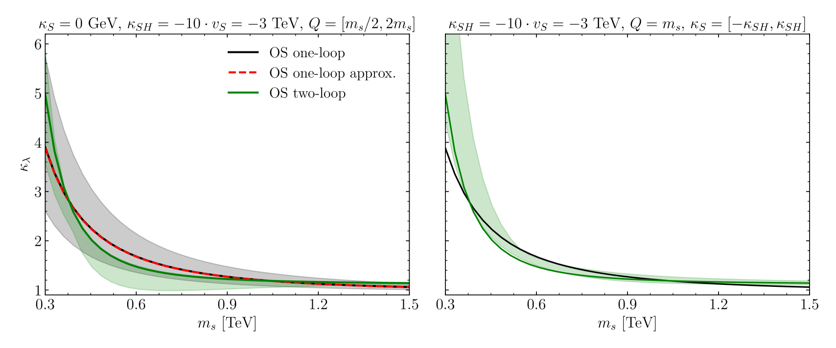
Figure 5: $\kappa_{\lambda}$ as a function of $m_{s}$ computed in the general singlet extension of the SM. Left: Comparison of the full one-loop (black solid curve), approximated one-loop (red dashed curve), and two-loop results (green solid curve) and their scale dependence. Right: Dependence of the two-loop result on $\kappa_{S}$.

In the left panel of ˜5, $\kappa_{\lambda}$ is shown as a function of $m_{s}$. The differences between the full one-loop (black solid, computed using anyH3 [14]) and the approximated one-loop (red dashed, setting $m_{h}=0$ in the one-loop corrections, cf. ˜76a) results are negligibly small, thus validating the approximation used for the calculation of the leading two-loop corrections (green solid). We note that at the tree level we always use $m_{h}=125\,\,\mathrm{GeV}$ since $m_{h}=0$ would introduce a rather large error. The two-loop corrections enhance $\kappa_{\lambda}$ by $\sim 1.2$ for $m_{s}\sim 300\,\,\mathrm{GeV}$ compared to the one-loop result. The shift induced by the two-loop corrections shrinks down for rising $m_{s}$ and then increases again for $m_{s}\gtrsim 800\,\,\mathrm{GeV}$. The reason why the asymptotic behaviour of the two-loop curve is different from the one-loop curve is that the singlet-specific one-loop corrections vanish for large $m_{s}$ while the corresponding two-loop corrections contain a part that is independent of $m_{s}$ but only suppressed by $v_{S}$, cf. the first term in ˜65. However, for a proper decoupling a relation of the form $v_{S}\propto m_{s}$ (or alternatively $\kappa_{S}=\kappa_{SH}=0$) is required, which induces the appropriate asymptotic behaviour. The left panel of ˜5 also shows the scale dependence of the one- and two-loop corrections induced by defining $\kappa_{SH}$ in the $\overline{\text{MS}}$ scheme (while all other parameters entering the one-loop correction are fixed in the OS scheme). The coloured bands are derived by varying the renormalisation scale between $Q=m_{s}/2$ and $Q=2m_{s}$, and using the leading-log approximation to relate $\kappa_{SH}(m_{S})$ to $\kappa_{SH}(Q)$. Although the scale dependence is very sizeable at the one-loop level, this dependence is significantly reduced when including the two-loop corrections, clearly showing their numerical importance — cf. the discussion around ˜67. Finally, in the right panel of ˜5, we investigate the dependence of the two-loop corrections on $\kappa_{S}$, which first enters at the two-loop level. We assess this dependence by varying $\kappa_{S}$ between $-\kappa_{SH}$ and $\kappa_{SH}$. We observe that the dependence on $\kappa_{S}$ is sizeable and especially pronounced for low $m_{s}$, while it shrinks down for higher $m_{s}$. However, even for high $m_{s}$, it remains of the same size as the difference between the one- and two-loop predictions for $\kappa_{\lambda}$ computed for $\kappa_{S}=0$. This illustrates the importance of this new class of two-loop corrections, which we have computed for the first time in this work.

6 Conclusions

The investigation of the Higgs potential is one of the main goals of the LHC programme and of future colliders. High-precision theoretical predictions are crucial to exploit the experimental constraints, or (in the future) measurements, on the trilinear and quartic Higgs couplings, in particular in order to understand implications for concrete BSM scenarios. As shown in the literature, one-loop predictions for the trilinear and quartic Higgs couplings are in this regard not sufficient for an accurate result. With this motivation in mind, we have presented a generic two-loop calculation of the scalar $n$-point functions (with $n\leq 4$) with identical external particles in the zero-momentum approximation. Besides the genuine two-loop contributions, we have also presented results for the occurring subloop-renormalisation contributions. Together, these constitute the necessary ingredients for calculations of the effective trilinear and quartic self-couplings of the detected Higgs boson, corresponding to the operators that are (or will be, for the quartic coupling) constrained by LHC data and can also be understood as operators in the Higgs Effective Field Theory (HEFT) [106, 107, 108, 109, 110, 111, 112, 113, 114, 115, 116, 117, 118, 119, 120, 121]. Building upon a unique canonical form of Feynman diagrams, we have demonstrated how the number of diagrams to compute can be reduced using symmetry relations. Moreover, we have worked out an on-the-fly reduction of the appearing loop integrals allowing for a stable numerical evaluation. These evaluation routines are available publicly in the form of the new Python package Tintegrals. Lastly, we have shown how our generic results can be mapped to amplitudes generated via FeynArts, thereby facilitating the application of our results to a wide range of theories. Using these routines, we have performed a series of cross-checks against existing results in the literature. Moreover, we have presented new two-loop results for the trilinear Higgs coupling in the general scalar singlet extension of the SM — these are in particular the first two-loop results for $\lambda_{hhh}$ including the effect of Lagrangian trilinear couplings. The obtained generic results are a core ingredient needed for automatic two-loop predictions of the trilinear and quartic Higgs couplings in arbitrary BSM models (e.g. in the anyH3 framework), which we leave for future endeavours. Our work also offers a base to build on to investigate high-precision predictions of Higgs (self-)couplings with non-vanishing external momenta, and to tackle the Goldstone Boson Catastrophe [122, 123, 124, 125, 126, 50] in this context.

Appendix A Loop-corrected scalar couplings in the general singlet extendion of the Standard Model

In this appendix, we renormalise the scalar sector of the general SSM in the approximation of vanishing tree-level mixing and of a heavy singlet mass. This is, in parts, required for the calculation of the two-loop shift presented in ˜5.

Renormalisation in the $\overline{\text{MS}}$ scheme:

As already mentioned in the main text, $\overline{\text{MS}}$ counterterms can in principle conveniently be derived from renormalisation group equations, which have been known for general renormalisable theories since a long time, see e.g. Machacek:1983tz,Machacek:1983fi,Machacek:1984zw,Sperling:2013xqa,Sperling:2013eva,Schienbein:2018fsw, and are available for concrete models in e.g. SARAH [98]. While this method can serve as a quite powerful cross-check of the UV-structure of the calculated diagrams (as we are introducing information from an independent calculation), it can have caveats in situations where approximations increase the number of scale-less integrals (as is the case in the calculation presented in this work) that we want to briefly comment on here. For demonstration purposes, we consider the scalar contributions to the one-loop beta function of $\kappa_{SH}$. The result computed by SARAH consists of three contributions

$$\beta^{(1)}_{\kappa_{SH}}=6\kappa_{SH}\lambda_{H}+2\kappa_{S}\lambda_{SH}+4\kappa_{SH}\lambda_{SH}\,,$$ (70)

which can be understood by considering the UV-divergent diagrams of the one-loop scalar contributions to the $SHH^{\dagger}$-coupling:

$$\delta^{(1)}\kappa_{SH}\sim 6\lambda_{H}\kappa_{SH}\textbf{B}_{0}(0,\mu^{2},\mu^{2})+2\lambda_{SH}\kappa_{S}\textbf{B}_{0}(0,\mu_{S}^{2},\mu_{S}^{2})+4\lambda_{SH}\kappa_{SH}\textbf{B}_{0}(0,\mu^{2},\mu^{2})$$ (71)

the first term originates in the diagram with two internal doublet scalars, which vanishes for $\lambda_{H}=0$. The second diagram contributes with two singlets in the loop. The third diagram has again two doublet scalars in the loop and is a permutation of the external legs of the first diagram. However, since $\mu^{2}=0$ (in our approximation) the third diagram is scale-less and therefore vanishes in dimensional regularisation. Thus, the actual beta function relevant for the applied approximations is just $\beta^{(1)}_{\kappa_{SH}}=2\kappa_{S}\lambda_{SH}$. Likewise, we find for the $\lambda_{S}$ beta function $\beta_{\lambda_{S}}^{(1)}=36\lambda_{S}^{2}$ instead of $\beta_{\lambda_{S}}^{(1)}=36\lambda_{S}^{2}+\lambda_{SH}^{2}$ even though we do not set $\lambda_{SH}$ to zero. Having set scale-less integrals consistently to zero across the entire calculation, we arrive at the following $\overline{\text{MS}}$ counterterms:

$$(4\pi)^{2}\delta^{(1)}_{\text{CT}}\kappa_{S}^{{\overline{\text{MS}}}} =\frac{18}{\epsilon}\kappa_{S}\lambda_{S}\,,$$ (72a)

$$(4\pi)^{2}\delta^{(1)}_{\text{CT}}\kappa_{SH}^{{\overline{\text{MS}}}} =\frac{\lambda_{SH}}{\epsilon}\left(\kappa_{S}+2\kappa_{SH}\right)\,,$$ (72b)

$$(4\pi)^{2}\delta^{(1)}_{\text{CT}}\lambda_{S}^{{\overline{\text{MS}}}} =\frac{18}{\epsilon}\lambda_{S}^{2}\,,$$ (72c)

$$(4\pi)^{2}\delta^{(1)}_{\text{CT}}\lambda_{H}^{{\overline{\text{MS}}}} =\frac{1}{2\epsilon}\lambda_{SH}^{2}\,,$$ (72d)

$$(4\pi)^{2}\delta^{(1)}_{\text{CT}}\lambda_{SH}^{{\overline{\text{MS}}}} =\frac{2\,\lambda_{SH}}{\epsilon}(3\lambda_{S}+\lambda_{SH})\,,$$ (72e)

at the one-loop and

$$\delta^{(2)}_{\text{CT}}\lambda_{H}^{{\overline{\text{MS}}}}=\frac{1}{(4\pi)^{4}}\left(\frac{1}{\epsilon^{2}}\lambda_{SH}^{2}(3\lambda_{S}+\lambda_{SH})-\frac{1}{2\epsilon}3\lambda_{SH}^{3}\right)\,.$$ (73)

at the two-loop order. Using these counterterms, we can compute the lower-order renormalised couplings required for ˜55:

$$\left.\hat{\lambda}^{(1)}_{hhh}\right|^{{\overline{\text{MS}}}} =\frac{v\kappa_{SH}^{2}}{2\,v_{S}^{3}(4\pi)^{2}}\left(\frac{v^{2}\kappa_{SH}}{m_{s}^{2}}-3v_{S}\overline{\ln}m_{s}^{2}\right)+\mathcal{O}(m_{h}^{2}/m_{s}^{2})\,,$$ (74a)

$$\left.\hat{\lambda}^{(1)}_{hhs}\right|^{{\overline{\text{MS}}}} =\frac{\kappa_{SH}}{2\,v_{S}^{3}(4\pi)^{2}}\left(v_{S}\overline{\ln}m_{s}^{2}-\frac{v^{2}\kappa_{SH}}{m_{s}^{2}}\right)\left(3m_{s}^{2}+\frac{3v^{2}\kappa_{SH}}{2v_{S}}-v_{S}\kappa_{S}\right)+\mathcal{O}(m_{h}^{2}/m_{s}^{2})\,,$$ (74b)

$$\lambda^{(0)}_{hss} =\frac{v}{v_{s}}\kappa_{SH}\,.$$ (74c)

and the appropriate LSZ factors consisting of the renormalised $\overline{\text{MS}}$ self-energies:

$$\left.Z_{hh}^{(1)}\right|^{{\overline{\text{MS}}}} =\frac{v^{2}\kappa_{SH}^{2}}{12v_{S}^{2}m_{s}^{2}(4\pi)^{2}}+\delta_{\rm CT}^{(1)}Z_{hh}\$$ (75a)

$$\left.Z_{hs}^{(1)}\right|^{{\overline{\text{MS}}}} =\frac{\hat{\Sigma}_{hs}(0)}{m_{s}^{2}}=\frac{1}{m_{s}^{2}}\left(\Sigma_{hs}(0)-v\,\delta_{\rm CT}^{(1)}\kappa_{SH}^{\overline{\text{MS}}}-v\,v_{S}\,\delta_{\rm CT}^{(1)}\lambda_{SH}^{\overline{\text{MS}}}-m_{s}^{2}\frac{\delta_{\rm CT}^{(1)}Z_{hs}}{2}\right)$$ (75b)

$$=\frac{v\kappa_{SH}}{2v_{S}^{2}m_{s}^{2}(4\pi)^{2}}\left(3m_{s}^{2}+\frac{3v^{2}\kappa_{SH}}{2v_{S}}-v_{S}\kappa_{S}\right)\overline{\ln}m_{s}^{2}-\frac{\delta_{\rm CT}^{(1)}Z_{hs}}{2}\,.$$ (75c)

Renormalisation in the OS scheme:

The OS one- and two-loop counterterms for the SSM are defined in ˜5. Their algebraic structure is rather involved and not particularly illuminating. Therefore, we only list analytic results required for the LSZ contributions, analogous to the $\overline{\text{MS}}$ scheme above. The relevant renormalised one-loop trilinear couplings read

$$\left.\hat{\lambda}^{(1)}_{hhh}\right|^{\text{OS}} =\frac{1}{(4\pi)^{2}}\frac{\kappa_{SH}^{3}v^{3}}{2v_{S}^{3}m_{s}^{2}}+\mathcal{O}(m_{h}^{2}/m_{s}^{2})\,,$$ (76a)

$$\left.\hat{\lambda}^{(1)}_{hhs}\right|^{\text{OS}} =-\frac{1}{(4\pi)^{2}}\frac{\kappa_{SH}^{2}v^{2}}{2v_{S}^{3}m_{s}^{2}}\left(3m_{s}^{2}+\frac{3\kappa_{SH}v^{2}}{2v_{S}}-v_{S}\kappa_{S}\right)+\mathcal{O}(m_{h}^{2}/m_{s}^{2})\,,$$ (76b)

whereas the finite LSZ factors are rather simple,

$$\left.Z_{hh}^{(1)}\right|^{\text{OS}} =\left.Z_{hh}^{(1)}\right|^{{\overline{\text{MS}}}}\,,$$ (77a)

$$\left.Z_{hs}^{(1)}\right|^{\text{OS}} =\frac{\delta_{\rm CT}^{(1)}Z_{hs}}{2}\,,$$ (77b)

due to the on-shell renormalisation of $\alpha$ which removes the $h-s$ mixing. The algebraic $\alpha$ counterterm, expanded to $\mathcal{O}(\epsilon^{1})$, is given by

$$\delta_{\rm CT}^{(1)}\alpha^{\text{OS}} =-\frac{\Sigma_{hs}(0)}{m_{s}^{2}}$$

$$=-\frac{v\kappa_{SH}}{2v_{S}^{2}m_{s}^{2}(4\pi)^{2}}\left(3m_{s}^{2}+\frac{3v^{2}\kappa_{SH}}{2v_{S}}-v_{S}\kappa_{S}\right)\left(\overline{\ln}m_{s}^{2}-\frac{1}{\epsilon}+\epsilon\,(1-\overline{\ln}m_{s}^{2})\right)\,,$$ (78)

where the finite part coincides with the off-diagonal LSZ factor in the $\overline{\text{MS}}$ scheme,

$$Z_{hs}^{(1)}\big{|}^{{\overline{\text{MS}}}}=-\delta_{\rm CT}^{(1)}\alpha^{{\text{OS}}}\,.$$

Validation:

To further check our calculational framework for consistency, we computed all renormalised scalar one-loop one-, two-, three-, and four-point functions of the SSM in both, the $\overline{\text{MS}}$ and the OS scheme and found UV-finite results. However, computing quantities at the $n$-loop level that implicitly involve $\mu_{S}$ at the $(n-1)$-loop level, such as e.g. $\hat{\Sigma}_{ss}^{(1)}$ or $\hat{\lambda}_{ssss}^{(1)}$, must be taken with care in the mixed OS-$\overline{\text{MS}}$ scheme since one has to distinguish between the OS counterterm for the singlet tadpole coefficient,

$$t_{s}=\left.\frac{\partial V_{\rm SSM}}{\partial s}\right|_{s=h=0}\,,$$ (79)

and the counterterm of the linear operator $\tilde{t}_{S}\cdot S$ in ˜48. While $\delta_{\rm CT}^{(1)}t_{s}$ appears e.g. in the renormalisation of $t_{h}$, cf. ˜62, the counterterm of $\mu_{S}$ is related to $t_{s}-\tilde{t}_{S}$ via the tree-level tadpole condition:

$$\mu_{S}=\frac{t_{s}-\tilde{t}_{S}}{v_{S}}-v_{S}(\kappa_{S}+2\lambda_{S}v_{S})-\frac{v^{2}}{2v_{S}}(\kappa_{SH}+\lambda_{SH}v_{S})\,.$$ (80)

Thus, $t_{s}$ and $\tilde{t}_{S}$ do not always appear in the same linear combination and need to be renormalised separately. Considering for example the UV-divergent part of the one-loop self-energy $\Sigma_{SS}$ in the gauge basis, we can compute a counterterm for $\mu_{S}$ and indeed find full agreement with the $\overline{\text{MS}}$ counterterm

$$(4\pi)^{2}\delta_{\rm CT}^{(1)}(\mu^{2})^{\overline{\text{MS}}}=(2\kappa_{S}^{2}+6\mu_{S}^{2}\lambda_{S})/\epsilon$$ (81)

extracted from the RGEs for $\mu_{S}$ computed with SARAH within our approximation (taking care of scale-less integrals as discussed above). Applying a counterterm transformation onto the right-hand side of ˜80 and using the $\overline{\text{MS}}$ counterterms in ˜72 as well as renormalising $t_{s}$ in the OS scheme, i.e.

$$\delta^{(1)}_{\rm CT}t_{s}^{{\text{OS}}}=-t_{s}^{(1)}=(\kappa_{S}+6\,v_{S}\lambda_{S})\textbf{A}_{0}(m_{s}^{2})\,,$$ (82)

we can solve for $\delta_{\rm CT}^{(1)}\tilde{t}_{S}$ and find

$$(4\pi)^{2}\delta_{\rm CT}^{(1)}\tilde{t}_{S}=\frac{\kappa_{S}}{2\epsilon}\left(v_{S}\,\kappa_{S}+\frac{v^{2}\kappa_{SH}}{2}+m_{s}^{2}\right)\,,$$ (83)

which is non-zero for $\kappa_{S}\neq 0$. Likewise, the linear combination $\delta_{\rm CT}^{(1)}\tilde{t}_{S}-\delta_{\rm CT}^{(1)}t_{s}$ enters the renormalisation of the singlet self-energy $\Sigma_{ss}$ and its cubic and quartic self-couplings, which are all rendered UV-finite by ˜83. It should be stressed that the choice of renormalising $\tilde{t}_{S}$ is not unique. It is related via a shift symmetry to the parameters $v_{S}$ and $\kappa_{S}$ which could equally be used to obtain UV-finite results.

Appendix B Tintegrals Python package

Tintegrals is a Python package to evaluate the $T$ integrals defined in Eq.˜2 numerically for vanishing external momenta. The Tintegrals source code is hosted at

https://gitlab.com/anybsm/tint.

The code is most easily used by installing the corresponding Python package by running

⬇

pip install Tintegrals

which will automatically download and install Tintegrals as well as the necessary dependencies. Running the code requires at least Python version 3.5. The Tintegrals module is loaded via e.g.

⬇

import Tintegrals as Tint

The module includes functions to numerically evaluate the UV-finite parts of all $T$ integrals needed to evaluate the generic expressions derived in this work. This implementation includes all the special cases derived during the integral reduction (see the discussion in Section˜2.4). To decide whether two masses, $m_{1}$ and $m_{2}$, should be considered numerically equal, the module checks whether

$$|m_{1}-m_{2}|<\rm{max}(\epsilon_{\text{rel}}(m_{1}+m_{2}),\epsilon_{\rm{diff}})\,.$$ (84)

where by default, $\epsilon_{\text{rel}}=10^{-10}$ and $\epsilon_{\text{diff}}=10^{-12}$. Using this criterion, the loop integrals are then evaluated e.g. via

⬇

Tint.setMudim(125**2)

Tint.T134fin(125, 125, 125)

where in the first step the renormalisation scale is set to $125\,\,\mathrm{GeV}$. In the second step, the value of the $T_{134}(m_{h},m_{h},m_{h})$ scalar integral for an internal mass of $125\,\,\mathrm{GeV}$ is calculated. Comprehensive documentation outlining the complete range of functions is accessible at

https://anybsm.gitlab.io/tint.

moreauthor morelabelname moreauthor morelabelname moreauthor morelabelname moreauthor morelabelname moreauthor morelabelname moreauthor morelabelname moreauthor morelabelname moreauthor morelabelname

References

- [1] Albert M Sirunyan “A measurement of the Higgs boson mass in the diphoton decay channel” In Phys. Lett. B 805, 2020, pp. 135425 DOI: 10.1016/j.physletb.2020.135425
- [2] Georges Aad “Measurement of the Higgs boson mass with H→ decays in 140 fb1 of s=13 TeV pp collisions with the ATLAS detector” In Phys. Lett. B 847, 2023, pp. 138315 DOI: 10.1016/j.physletb.2023.138315
- [3] Benjamin Fuks, Jeong Han Kim and Seung J. Lee “Scrutinizing the Higgs quartic coupling at a future 100 TeV proton–proton collider with taus and b-jets” In Phys. Lett. B 771, 2017, pp. 354–358 DOI: 10.1016/j.physletb.2017.05.075
- [4] Andreas Papaefstathiou, Tania Robens and Gilberto Tetlalmatzi-Xolocotzi “Triple Higgs Boson Production at the Large Hadron Collider with Two Real Singlet Scalars” In JHEP 05, 2021, pp. 193 DOI: 10.1007/JHEP05(2021)193
- [5] Panagiotis Stylianou and Georg Weiglein “Constraints on the trilinear and quartic Higgs couplings from triple Higgs production at the LHC and beyond”, 2023 arXiv:2312.04646 [hep-ph]
- [6] Vuko Brigljevic “HHH Whitepaper” In HHH Workshop, 2024 arXiv:2407.03015 [hep-ph]
- [7] Georges Aad “Combination of Searches for Higgs Boson Pair Production in pp Collisions at s=13 TeV with the ATLAS Detector” In Phys. Rev. Lett. 133.10, 2024, pp. 101801 DOI: 10.1103/PhysRevLett.133.101801
- [8] dummy “Constraining the Higgs boson self-coupling from single- and double-Higgs production with the ATLAS detector using collisions at TeV”, 2022
- [9] dummy “A portrait of the Higgs boson by the CMS experiment ten years after the discovery” In Nature 607.7917, 2022, pp. 60–68 DOI: 10.1038/s41586-022-04892-x
- [10] dummy “Constraining the Higgs boson self-coupling from single- and double-Higgs production with the ATLAS detector using collisions at TeV”, 2022 arXiv:2211.01216 [hep-ex]
- [11] Aram Hayrapetyan “Constraints on the Higgs boson self-coupling from the combination of single and double Higgs boson production in proton-proton collisions at = 13 TeV”, 2024 arXiv:2407.13554 [hep-ex]
- [12] J. Baglio et al. “ : Combined uncertainties” In Phys. Rev. D 103.5, 2021, pp. 056002 DOI: 10.1103/PhysRevD.103.056002
- [13] Henning Bahl, Johannes Braathen and Georg Weiglein “New Constraints on Extended Higgs Sectors from the Trilinear Higgs Coupling” In Phys. Rev. Lett. 129.23, 2022, pp. 231802 DOI: 10.1103/PhysRevLett.129.231802
- [14] Henning Bahl, Johannes Braathen, Martin Gabelmann and Georg Weiglein “anyH3: precise predictions for the trilinear Higgs coupling in the Standard Model and beyond” [Erratum: Eur.Phys.J.C 84, 498 (2024)] In Eur. Phys. J. C 83.12, 2023, pp. 1156 DOI: 10.1140/epjc/s10052-023-12173-8
- [15] J. Blas “Higgs Boson Studies at Future Particle Colliders”, 2019 arXiv:1905.03764 [hep-ph]
- [16] M. Cepeda “Higgs Physics at the HL-LHC and HE-LHC”, 2019 arXiv:1902.00134 [hep-ph]
- [17] Vernon D. Barger, M.. Berger, A.. Stange and R… Phillips “Supersymmetric Higgs boson hadroproduction and decays including radiative corrections” In Phys. Rev. D45, 1992, pp. 4128–4147 DOI: 10.1103/PhysRevD.45.4128
- [18] Wolfgang Hollik and Siannah Penaranda “Yukawa coupling quantum corrections to the selfcouplings of the lightest MSSM Higgs boson” In Eur. Phys. J. C23, 2002, pp. 163–172 DOI: 10.1007/s100520100862
- [19] Antonio Dobado, Maria J. Herrero, Wolfgang Hollik and Siannah Penaranda “Selfinteractions of the lightest MSSM Higgs boson in the large pseudoscalar mass limit” In Phys. Rev. D66, 2002, pp. 095016 DOI: 10.1103/PhysRevD.66.095016
- [20] K.. Williams and G. Weiglein “Precise predictions for decays in the complex MSSM” In Phys. Lett. B 660, 2008, pp. 217–227 DOI: 10.1016/j.physletb.2007.12.049
- [21] Karina E. Williams, Heidi Rzehak and Georg Weiglein “Higher order corrections to Higgs boson decays in the MSSM with complex parameters” In Eur. Phys. J. C 71, 2011, pp. 1669 DOI: 10.1140/epjc/s10052-011-1669-3
- [22] Shinya Kanemura, Mariko Kikuchi and Kei Yagyu “Radiative corrections to the Higgs boson couplings in the model with an additional real singlet scalar field” In Nucl. Phys. B907, 2016, pp. 286–322 DOI: 10.1016/j.nuclphysb.2016.04.005
- [23] Shinya Kanemura, Mariko Kikuchi and Kei Yagyu “One-loop corrections to the Higgs self-couplings in the singlet extension” In Nucl. Phys. B917, 2017, pp. 154–177 DOI: 10.1016/j.nuclphysb.2017.02.004
- [24] Shi-Ping He and Shou-hua Zhu “One-Loop Radiative Correction to the Triple Higgs Coupling in the Higgs Singlet Model” In Phys. Lett. B764, 2017, pp. 31–37 DOI: 10.1016/j.physletb.2016.11.007
- [25] Shinya Kanemura, Mariko Kikuchi, Kodai Sakurai and Kei Yagyu “Gauge invariant one-loop corrections to Higgs boson couplings in non-minimal Higgs models” In Phys. Rev. D96.3, 2017, pp. 035014 DOI: 10.1103/PhysRevD.96.035014
- [26] Shinya Kanemura et al. “New physics effect on the Higgs selfcoupling” In Phys. Lett. B558, 2003, pp. 157–164 DOI: 10.1016/S0370-2693(03)00268-5
- [27] Shinya Kanemura, Yasuhiro Okada, Eibun Senaha and C.-P. Yuan “Higgs coupling constants as a probe of new physics” In Phys. Rev. D70, 2004, pp. 115002 DOI: 10.1103/PhysRevD.70.115002
- [28] Shinya Kanemura, Mariko Kikuchi and Kei Yagyu “Fingerprinting the extended Higgs sector using one-loop corrected Higgs boson couplings and future precision measurements” In Nucl. Phys. B896, 2015, pp. 80–137 DOI: 10.1016/j.nuclphysb.2015.04.015
- [29] Abdesslam Arhrib, Rachid Benbrik, Jaouad El Falaki and Adil Jueid “Radiative corrections to the Triple Higgs Coupling in the Inert Higgs Doublet Model” In JHEP 12, 2015, pp. 007 DOI: 10.1007/JHEP12(2015)007
- [30] Shinya Kanemura, Mariko Kikuchi and Kodai Sakurai “Testing the dark matter scenario in the inert doublet model by future precision measurements of the Higgs boson couplings” In Phys. Rev. D94.11, 2016, pp. 115011 DOI: 10.1103/PhysRevD.94.115011
- [31] Jaouad El Falaki “Revisiting one-loop corrections to the trilinear Higgs boson self-coupling in the Inert Doublet Model”, 2023 arXiv:2301.13773 [hep-ph]
- [32] Mayumi Aoki, Shinya Kanemura, Mariko Kikuchi and Kei Yagyu “Radiative corrections to the Higgs boson couplings in the triplet model” In Phys. Rev. D87.1, 2013, pp. 015012 DOI: 10.1103/PhysRevD.87.015012
- [33] Cheng-Wei Chiang, An-Li Kuo and Kei Yagyu “One-loop renormalized Higgs boson vertices in the Georgi-Machacek model” In Phys. Rev. D 98.1, 2018, pp. 013008 DOI: 10.1103/PhysRevD.98.013008
- [34] Henning Bahl et al. “Tripling down on the boson mass” In Eur. Phys. J. C 82.10, 2022, pp. 944 DOI: 10.1140/epjc/s10052-022-10934-5
- [35] Shinya Kanemura, Mariko Kikuchi, Kodai Sakurai and Kei Yagyu “H-COUP: a program for one-loop corrected Higgs boson couplings in non-minimal Higgs sectors” In Comput. Phys. Commun. 233, 2018, pp. 134–144 DOI: 10.1016/j.cpc.2018.06.012
- [36] Shinya Kanemura et al. “H-COUP Version 2: a program for one-loop corrected Higgs boson decays in non-minimal Higgs sectors” In Comput. Phys. Commun. 257, 2020, pp. 107512 DOI: 10.1016/j.cpc.2020.107512
- [37] Masashi Aiko et al. “H-COUP Version 3: A program for one-loop corrected decays of any Higgs bosons in non-minimal Higgs models”, 2023 arXiv:2311.15892 [hep-ph]
- [38] Philipp Basler and Margarete Mühlleitner “BSMPT (Beyond the Standard Model Phase Transitions): A tool for the electroweak phase transition in extended Higgs sectors” In Comput. Phys. Commun. 237, 2019, pp. 62–85 DOI: 10.1016/j.cpc.2018.11.006
- [39] Philipp Basler, Margarete Mühlleitner and Jonas Müller “BSMPT v2 a tool for the electroweak phase transition and the baryon asymmetry of the universe in extended Higgs Sectors” In Comput. Phys. Commun. 269, 2021, pp. 108124 DOI: 10.1016/j.cpc.2021.108124
- [40] Philipp Basler et al. “BSMPT v3 A Tool for Phase Transitions and Primordial Gravitational Waves in Extended Higgs Sectors”, 2024 arXiv:2404.19037 [hep-ph]
- [41] Dao Thi Nhung, Margarete Muhlleitner, Juraj Streicher and Kathrin Walz “Higher Order Corrections to the Trilinear Higgs Self-Couplings in the Real NMSSM” In JHEP 11, 2013, pp. 181 DOI: 10.1007/JHEP11(2013)181
- [42] Eibun Senaha “Radiative Corrections to Triple Higgs Coupling and Electroweak Phase Transition: Beyond One-loop Analysis” In Phys. Rev. D100.5, 2019, pp. 055034 DOI: 10.1103/PhysRevD.100.055034
- [43] Johannes Braathen and Shinya Kanemura “On two-loop corrections to the Higgs trilinear coupling in models with extended scalar sectors” In Phys. Lett. B796, 2019, pp. 38–46 DOI: 10.1016/j.physletb.2019.07.021
- [44] Johannes Braathen and Shinya Kanemura “Leading two-loop corrections to the Higgs boson self-couplings in models with extended scalar sectors” In Eur. Phys. J. C 80.3, 2020, pp. 227 DOI: 10.1140/epjc/s10052-020-7723-2
- [45] Johannes Braathen, Shinya Kanemura and Makoto Shimoda “Two-loop analysis of classically scale-invariant models with extended Higgs sectors” In JHEP 03, 2021, pp. 297 DOI: 10.1007/JHEP03(2021)297
- [46] Masashi Aiko, Johannes Braathen and Shinya Kanemura “Leading two-loop corrections to the Higgs di-photon decay in the Inert Doublet Model”, 2023 arXiv:2307.14976 [hep-ph]
- [47] Mathias Brucherseifer, Ryan Gavin and Michael Spira “Minimal supersymmetric Higgs boson self-couplings: Two-loop corrections” In Phys. Rev. D90.11, 2014, pp. 117701 DOI: 10.1103/PhysRevD.90.117701
- [48] M. Mühlleitner, Dao Thi Nhung and Hanna Ziesche “The order corrections to the trilinear Higgs self-couplings in the complex NMSSM” In JHEP 12, 2015, pp. 034 DOI: 10.1007/JHEP12(2015)034
- [49] Christoph Borschensky et al. “The trilinear Higgs self-couplings at in the CP-violating NMSSM” In Eur. Phys. J. C 83.2, 2023, pp. 118 DOI: 10.1140/epjc/s10052-023-11215-5
- [50] Mark D. Goodsell and Sebastian Paßehr “All two-loop scalar self-energies and tadpoles in general renormalisable field theories” In Eur. Phys. J. C 80.5, 2020, pp. 417 DOI: 10.1140/epjc/s10052-020-7657-8
- [51] Stephen P. Martin “Two loop effective potential for a general renormalizable theory and softly broken supersymmetry” In Phys. Rev. D65, 2002, pp. 116003 DOI: 10.1103/PhysRevD.65.116003
- [52] Stephen P. Martin “Two loop scalar self energies in a general renormalizable theory at leading order in gauge couplings” In Phys. Rev. D70, 2004, pp. 016005 DOI: 10.1103/PhysRevD.70.016005
- [53] Stephen P. Martin “Evaluation of two loop selfenergy basis integrals using differential equations” In Phys. Rev. D68, 2003, pp. 075002 DOI: 10.1103/PhysRevD.68.075002
- [54] Stephen P. Martin and Hiren H. Patel “Two-loop effective potential for generalized gauge fixing” In Phys. Rev. D98.7, 2018, pp. 076008 DOI: 10.1103/PhysRevD.98.076008
- [55] M. Goodsell, K. Nickel and F. Staub “Generic two-loop Higgs mass calculation from a diagrammatic approach” In Eur. Phys. J. C75.6, 2015, pp. 290 DOI: 10.1140/epjc/s10052-015-3494-6
- [56] Florian Staub “SARAH 4 : A tool for (not only SUSY) model builders” In Comput. Phys. Commun. 185, 2014, pp. 1773–1790 DOI: 10.1016/j.cpc.2014.02.018
- [57] Florian Staub “Exploring new models in all detail with SARAH” In Adv. High Energy Phys. 2015, 2015, pp. 840780 DOI: 10.1155/2015/840780
- [58] Emanuele Bagnaschi, Javier Pardo Vega and Pietro Slavich “Improved determination of the Higgs mass in the MSSM with heavy superpartners” In Eur. Phys. J. C 77.5, 2017, pp. 334 DOI: 10.1140/epjc/s10052-017-4885-7
- [59] Peter Athron et al. “FlexibleSUSY 2.0: Extensions to investigate the phenomenology of SUSY and non-SUSY models” In Comput. Phys. Commun. 230, 2018, pp. 145–217 DOI: 10.1016/j.cpc.2018.04.016
- [60] Henning Bahl and Wolfgang Hollik “Precise prediction of the MSSM Higgs boson masses for low MA” In JHEP 07, 2018, pp. 182 DOI: 10.1007/JHEP07(2018)182
- [61] Johannes Braathen, Mark D. Goodsell and Pietro Slavich “Matching renormalisable couplings: simple schemes and a plot” In Eur. Phys. J. C 79.8, 2019, pp. 669 DOI: 10.1140/epjc/s10052-019-7093-9
- [62] Martin Gabelmann, Margarete Mühlleitner and Florian Staub “Automatised matching between two scalar sectors at the one-loop level” In Eur. Phys. J. C 79.2, 2019, pp. 163 DOI: 10.1140/epjc/s10052-019-6570-5
- [63] Henning Bahl and Ivan Sobolev “Two-loop matching of renormalizable operators: general considerations and applications” In JHEP 03, 2021, pp. 286 DOI: 10.1007/JHEP03(2021)286
- [64] P. Slavich “Higgs-mass predictions in the MSSM and beyond” In Eur. Phys. J. C 81.5, 2021, pp. 450 DOI: 10.1140/epjc/s10052-021-09198-2
- [65] Emanuele Bagnaschi, Giuseppe Degrassi, Sebastian Paßehr and Pietro Slavich “Full two-loop QCD corrections to the Higgs mass in the MSSM with heavy superpartners” In Eur. Phys. J. C 79.11, 2019, pp. 910 DOI: 10.1140/epjc/s10052-019-7417-9
- [66] T. Binoth and G. Heinrich “An automatized algorithm to compute infrared divergent multiloop integrals” In Nucl. Phys. B 585, 2000, pp. 741–759 DOI: 10.1016/S0550-3213(00)00429-6
- [67] T. Binoth and G. Heinrich “Numerical evaluation of multiloop integrals by sector decomposition” In Nucl. Phys. B 680, 2004, pp. 375–388 DOI: 10.1016/j.nuclphysb.2003.12.023
- [68] Christian Bogner and Stefan Weinzierl “Resolution of singularities for multi-loop integrals” In Comput. Phys. Commun. 178, 2008, pp. 596–610 DOI: 10.1016/j.cpc.2007.11.012
- [69] Gudrun Heinrich “Sector Decomposition” In Int. J. Mod. Phys. A 23, 2008, pp. 1457–1486 DOI: 10.1142/S0217751X08040263
- [70] S. Borowka et al. “pySecDec: a toolbox for the numerical evaluation of multi-scale integrals” In Comput. Phys. Commun. 222, 2018, pp. 313–326 DOI: 10.1016/j.cpc.2017.09.015
- [71] Francesco Moriello “Generalised power series expansions for the elliptic planar families of Higgs + jet production at two loops” In JHEP 01, 2020, pp. 150 DOI: 10.1007/JHEP01(2020)150
- [72] Michael Borinsky “Tropical Monte Carlo quadrature for Feynman integrals” In Ann. Inst. H. Poincare D Comb. Phys. Interact. 10.4, 2023, pp. 635–685 DOI: 10.4171/aihpd/158
- [73] A.. Smirnov, N.. Shapurov and L.. Vysotsky “FIESTA5: Numerical high-performance Feynman integral evaluation” In Comput. Phys. Commun. 277, 2022, pp. 108386 DOI: 10.1016/j.cpc.2022.108386
- [74] Xiao Liu and Yan-Qing Ma “AMFlow: A Mathematica package for Feynman integrals computation via auxiliary mass flow” In Comput. Phys. Commun. 283, 2023, pp. 108565 DOI: 10.1016/j.cpc.2022.108565
- [75] Michael Borinsky, Henrik J. Munch and Felix Tellander “Tropical Feynman integration in the Minkowski regime” In Comput. Phys. Commun. 292, 2023, pp. 108874 DOI: 10.1016/j.cpc.2023.108874
- [76] G. Heinrich et al. “Numerical scattering amplitudes with pySecDec” In Comput. Phys. Commun. 295, 2024, pp. 108956 DOI: 10.1016/j.cpc.2023.108956
- [77] J. Kublbeck, M. Bohm and Ansgar Denner “Feyn Arts: Computer Algebraic Generation of Feynman Graphs and Amplitudes” In Comput. Phys. Commun. 60, 1990, pp. 165–180 DOI: 10.1016/0010-4655(90)90001-H
- [78] Thomas Hahn “Generating Feynman diagrams and amplitudes with FeynArts 3” In Comput. Phys. Commun. 140, 2001, pp. 418–431 DOI: 10.1016/S0010-4655(01)00290-9
- [79] G. Weiglein, R. Scharf and M. Bohm “Reduction of general two loop selfenergies to standard scalar integrals” In Nucl. Phys. B 416, 1994, pp. 606–644 DOI: 10.1016/0550-3213(94)90325-5
- [80] G. Weiglein, R. Mertig, R. Scharf and M. Bohm “Computer algebraic calculation of two loop selfenergies in the electroweak standard model” In 2nd International Workshop on Software Engineering, Artificial Intelligence and Expert Systems for High-energy and Nuclear Physics, 1995
- [81] S. Heinemeyer, W. Hollik and G. Weiglein “FeynHiggs: A Program for the calculation of the masses of the neutral CP even Higgs bosons in the MSSM” In Comput. Phys. Commun. 124, 2000, pp. 76–89 DOI: 10.1016/S0010-4655(99)00364-1
- [82] S. Heinemeyer, W. Hollik and G. Weiglein “The Masses of the neutral CP - even Higgs bosons in the MSSM: Accurate analysis at the two loop level” In Eur. Phys. J. C 9, 1999, pp. 343–366 DOI: 10.1007/s100529900006
- [83] T. Hahn et al. “FeynHiggs: A program for the calculation of MSSM Higgs-boson observables - Version 2.6.5” In Comput. Phys. Commun. 180, 2009, pp. 1426–1427 DOI: 10.1016/j.cpc.2009.02.014
- [84] G. Degrassi et al. “Towards high precision predictions for the MSSM Higgs sector” In Eur. Phys. J. C 28, 2003, pp. 133–143 DOI: 10.1140/epjc/s2003-01152-2
- [85] M. Frank et al. “The Higgs Boson Masses and Mixings of the Complex MSSM in the Feynman-Diagrammatic Approach” In JHEP 02, 2007, pp. 047 DOI: 10.1088/1126-6708/2007/02/047
- [86] T. Hahn et al. “High-Precision Predictions for the Light CP -Even Higgs Boson Mass of the Minimal Supersymmetric Standard Model” In Phys. Rev. Lett. 112.14, 2014, pp. 141801 DOI: 10.1103/PhysRevLett.112.141801
- [87] Henning Bahl and Wolfgang Hollik “Precise prediction for the light MSSM Higgs boson mass combining effective field theory and fixed-order calculations” In Eur. Phys. J. C 76.9, 2016, pp. 499 DOI: 10.1140/epjc/s10052-016-4354-8
- [88] Henning Bahl, Sven Heinemeyer, Wolfgang Hollik and Georg Weiglein “Reconciling EFT and hybrid calculations of the light MSSM Higgs-boson mass” In Eur. Phys. J. C 78.1, 2018, pp. 57 DOI: 10.1140/epjc/s10052-018-5544-3
- [89] H. Bahl et al. “Precision calculations in the MSSM Higgs-boson sector with FeynHiggs 2.14” In Comput. Phys. Commun. 249, 2020, pp. 107099 DOI: 10.1016/j.cpc.2019.107099
- [90] G. Passarino and M… Veltman “One Loop Corrections for e+ e- Annihilation Into mu+ mu- in the Weinberg Model” In Nucl. Phys. B160, 1979, pp. 151–207 DOI: 10.1016/0550-3213(79)90234-7
- [91] T. Hahn and M. Perez-Victoria “Automatized one loop calculations in four-dimensions and D-dimensions” In Comput. Phys. Commun. 118, 1999, pp. 153–165 DOI: 10.1016/S0010-4655(98)00173-8
- [92] Thomas Hahn, Sebastian Paßehr and Christian Schappacher “FormCalc 9 and Extensions” In PoS LL2016, 2016, pp. 068 DOI: 10.1088/1742-6596/762/1/012065
- [93] Johannes Braathen et al. “-loop running should be combined with -loop matching” In Phys. Rev. D97.1, 2018, pp. 015011 DOI: 10.1103/PhysRevD.97.015011
- [94] J. Baglio et al. “NMSSMCALC: A Program Package for the Calculation of Loop-Corrected Higgs Boson Masses and Decay Widths in the (Complex) NMSSM” In Comput. Phys. Commun. 185.12, 2014, pp. 3372–3391 DOI: 10.1016/j.cpc.2014.08.005
- [95] Jose R. Espinosa, Thomas Konstandin and Francesco Riva “Strong Electroweak Phase Transitions in the Standard Model with a Singlet” In Nucl. Phys. B854, 2012, pp. 592–630 DOI: 10.1016/j.nuclphysb.2011.09.010
- [96] F. Staub “SARAH”, 2008 arXiv:0806.0538 [hep-ph]
- [97] Florian Staub “From Superpotential to Model Files for FeynArts and CalcHep/CompHep” In Comput. Phys. Commun. 181, 2010, pp. 1077–1086 DOI: 10.1016/j.cpc.2010.01.011
- [98] Florian Staub “Automatic Calculation of supersymmetric Renormalization Group Equations and Self Energies” In Comput. Phys. Commun. 182, 2011, pp. 808–833 DOI: 10.1016/j.cpc.2010.11.030
- [99] Florian Staub “SARAH 3.2: Dirac Gauginos, UFO output, and more” In Comput. Phys. Commun. 184, 2013, pp. 1792–1809 DOI: 10.1016/j.cpc.2013.02.019
- [100] Stephen P. Martin and David G. Robertson “Higgs boson mass in the Standard Model at two-loop order and beyond” In Phys. Rev. D90.7, 2014, pp. 073010 DOI: 10.1103/PhysRevD.90.073010
- [101] Stephen P. Martin “Pole Mass of the W Boson at Two-Loop Order in the Pure Scheme” In Phys. Rev. D 91.11, 2015, pp. 114003 DOI: 10.1103/PhysRevD.91.114003
- [102] Stephen P. Martin “-Boson Pole Mass at Two-Loop Order in the Pure Scheme” In Phys. Rev. D 92.1, 2015, pp. 014026 DOI: 10.1103/PhysRevD.92.014026
- [103] Stephen P. Martin “Top-quark pole mass in the tadpole-free scheme” In Phys. Rev. D93.9, 2016, pp. 094017 DOI: 10.1103/PhysRevD.93.094017
- [104] Stephen P. Martin “Matching relations for decoupling in the Standard Model at two loops and beyond” In Phys. Rev. D 99.3, 2019, pp. 033007 DOI: 10.1103/PhysRevD.99.033007
- [105] Ansgar Denner, Stefan Dittmaier and Jean-Nicolas Lang “Renormalization of mixing angles” In JHEP 11, 2018, pp. 104 DOI: 10.1007/JHEP11(2018)104
- [106] F. Feruglio “The Chiral approach to the electroweak interactions” In Int. J. Mod. Phys. A 8, 1993, pp. 4937–4972 DOI: 10.1142/S0217751X93001946
- [107] C.. Burgess, J. Matias and M. Pospelov “A Higgs or not a Higgs? What to do if you discover a new scalar particle” In Int. J. Mod. Phys. A 17, 2002, pp. 1841–1918 DOI: 10.1142/S0217751X02009813
- [108] G.. Giudice, C. Grojean, A. Pomarol and R. Rattazzi “The Strongly-Interacting Light Higgs” In JHEP 06, 2007, pp. 045 DOI: 10.1088/1126-6708/2007/06/045
- [109] Benjamin Grinstein and Michael Trott “A Higgs-Higgs bound state due to new physics at a TeV” In Phys. Rev. D 76, 2007, pp. 073002 DOI: 10.1103/PhysRevD.76.073002
- [110] R. Alonso et al. “The Effective Chiral Lagrangian for a Light Dynamical ”Higgs Particle”” [Erratum: Phys.Lett.B 726, 926 (2013)] In Phys. Lett. B 722, 2013, pp. 330–335 DOI: 10.1016/j.physletb.2013.04.037
- [111] Aleksandr Azatov, Roberto Contino and Jamison Galloway “Model-Independent Bounds on a Light Higgs” [Erratum: JHEP 04, 140 (2013)] In JHEP 04, 2012, pp. 127 DOI: 10.1007/JHEP04(2012)127
- [112] Gerhard Buchalla and Oscar Cata “Effective Theory of a Dynamically Broken Electroweak Standard Model at NLO” In JHEP 07, 2012, pp. 101 DOI: 10.1007/JHEP07(2012)101
- [113] Roberto Contino et al. “Effective Lagrangian for a light Higgs-like scalar” In JHEP 07, 2013, pp. 035 DOI: 10.1007/JHEP07(2013)035
- [114] Gerhard Buchalla, Oscar Catà and Claudius Krause “Complete Electroweak Chiral Lagrangian with a Light Higgs at NLO” [Erratum: Nucl.Phys.B 913, 475–478 (2016)] In Nucl. Phys. B 880, 2014, pp. 552–573 DOI: 10.1016/j.nuclphysb.2014.01.018
- [115] Rodrigo Alonso, Elizabeth E. Jenkins and Aneesh V. Manohar “Holomorphy without Supersymmetry in the Standard Model Effective Field Theory” In Phys. Lett. B 739, 2014, pp. 95–98 DOI: 10.1016/j.physletb.2014.10.045
- [116] Feng-Kun Guo, Pedro Ruiz-Femen´ıa and Juan José Sanz-Cillero “One loop renormalization of the electroweak chiral Lagrangian with a light Higgs boson” In Phys. Rev. D 92, 2015, pp. 074005 DOI: 10.1103/PhysRevD.92.074005
- [117] G. Buchalla, O. Cata, A. Celis and C. Krause “Fitting Higgs Data with Nonlinear Effective Theory” In Eur. Phys. J. C 76.5, 2016, pp. 233 DOI: 10.1140/epjc/s10052-016-4086-9
- [118] G. Buchalla et al. “Complete One-Loop Renormalization of the Higgs-Electroweak Chiral Lagrangian” In Nucl. Phys. B 928, 2018, pp. 93–106 DOI: 10.1016/j.nuclphysb.2018.01.009
- [119] G. Buchalla et al. “Higgs boson pair production in non-linear Effective Field Theory with full -dependence at NLO QCD” In JHEP 09, 2018, pp. 057 DOI: 10.1007/JHEP09(2018)057
- [120] Adam Falkowski and Riccardo Rattazzi “Which EFT” In JHEP 10, 2019, pp. 255 DOI: 10.1007/JHEP10(2019)255
- [121] Timothy Cohen, Nathaniel Craig, Xiaochuan Lu and Dave Sutherland “Is SMEFT Enough?” In JHEP 03, 2021, pp. 237 DOI: 10.1007/JHEP03(2021)237
- [122] J. Elias-Miro, J.. Espinosa and T. Konstandin “Taming Infrared Divergences in the Effective Potential” In JHEP 08, 2014, pp. 034 DOI: 10.1007/JHEP08(2014)034
- [123] Stephen P. Martin “Taming the Goldstone contributions to the effective potential” In Phys. Rev. D90.1, 2014, pp. 016013 DOI: 10.1103/PhysRevD.90.016013
- [124] Nilanjana Kumar and Stephen P. Martin “Resummation of Goldstone boson contributions to the MSSM effective potential” In Phys. Rev. D94.1, 2016, pp. 014013 DOI: 10.1103/PhysRevD.94.014013
- [125] Johannes Braathen and Mark D. Goodsell “Avoiding the Goldstone Boson Catastrophe in general renormalisable field theories at two loops” In JHEP 12, 2016, pp. 056 DOI: 10.1007/JHEP12(2016)056
- [126] Johannes Braathen, Mark D. Goodsell and Florian Staub “Supersymmetric and non-supersymmetric models without catastrophic Goldstone bosons” In Eur. Phys. J. C77.11, 2017, pp. 757 DOI: 10.1140/epjc/s10052-017-5303-x
- [127] Marie E. Machacek and Michael T. Vaughn “Two Loop Renormalization Group Equations in a General Quantum Field Theory. 1. Wave Function Renormalization” In Nucl. Phys. B 222, 1983, pp. 83–103 DOI: 10.1016/0550-3213(83)90610-7
- [128] Marie E. Machacek and Michael T. Vaughn “Two Loop Renormalization Group Equations in a General Quantum Field Theory. 2. Yukawa Couplings” In Nucl. Phys. B 236, 1984, pp. 221–232 DOI: 10.1016/0550-3213(84)90533-9
- [129] Marie E. Machacek and Michael T. Vaughn “Two Loop Renormalization Group Equations in a General Quantum Field Theory. 3. Scalar Quartic Couplings” In Nucl. Phys. B 249, 1985, pp. 70–92 DOI: 10.1016/0550-3213(85)90040-9
- [130] Marcus Sperling, Dominik Stöckinger and Alexander Voigt “Renormalization of vacuum expectation values in spontaneously broken gauge theories: Two-loop results” In JHEP 01, 2014, pp. 068 DOI: 10.1007/JHEP01(2014)068
- [131] Marcus Sperling, Dominik Stöckinger and Alexander Voigt “Renormalization of vacuum expectation values in spontaneously broken gauge theories” In JHEP 07, 2013, pp. 132 DOI: 10.1007/JHEP07(2013)132
- [132] Ingo Schienbein, Florian Staub, Tom Steudtner and Kseniia Svirina “Revisiting RGEs for general gauge theories” [Erratum: Nucl.Phys.B 966, 115339 (2021)] In Nucl. Phys. B 939, 2019, pp. 1–48 DOI: 10.1016/j.nuclphysb.2018.12.001