Using machine learning to measure evidence of students’ sensemaking in physics courses

Abstract

In the education system, problem-solving correctness is often inappropriately conflated with student learning. Advances in both Physics Education Research (PER) and Machine Learning (ML) provide the initial tools to develop a more meaningful and efficient measurement scheme for whether physics students are engaging in sensemaking: a learning process of figuring out the “how” and “why” for a particular phenomena. In this work, we contribute such a measurement scheme, which quantifies the evidence of students’ physical sensemaking given their written explanations for their solutions to physics problems. We outline how the proposed human annotation scheme can be automated into a deployable ML model using language encoders and shared probabilistic classifiers. The procedure is scalable for a large number of problems and students. We implement three unique language encoders with logistic regression, and provide a deployability analysis on $385$ real student explanations from the 2023 Introduction to Physics course at Tufts University. Furthermore, we compute sensemaking scores for all students, and analyze these measurements alongside their corresponding problem-solving accuracies. We find no linear relationship between these two variables, supporting the hypothesis that one is not a reliable proxy for the other. We discuss how sensemaking scores can be used alongside problem-solving accuracies to provide a more nuanced snapshot of student performance in physics class.

I Introduction

Teaching and instruction in undergraduate physics courses has largely relied on problem-solving as the standard method to measure student performance [1, 2, 3, 4, 5, 6]. Common practice is for “real-time” performance to be measured via multiple-choice or single-solution problems, where canonically correct answers determine the student’s knowledge of the core material. Accuracy scores across assignments and examinations, typically coupled with letter grades, act as signals of progress throughout the course as well as final verdicts of student success.

While problem-solving is a useful skill in a physics classroom, using the problem solution as a measure of student learning assumes a direct correlation that may not always hold. Problem-solving accuracy as a measurand assumes that students will engage in a learning process involving the core material to obtain the problem solution. Often times, there are alternative strategies for obtaining a problem solution such as rote-memorization of the rules or procedures required for solving similar problem types [7]. In this scenario, students would score very high on exams that contain these problem types; however given a previously unseen problem structure where the same core material is to be applied, the students would struggle. Here, a risk of using problem-solving accuracy as the predominant metric is an inflated sense of confidence in both the instructor and the student that the core material has been learned. It could also pose a risk for confounding variables in research studies that aim to investigate how instructional techniques influence student learning [8, 9, 10, 11, 12].

Over the last fifteen years, researchers in STEM Education (Ed.) have focused more closely on modeling a student’s learning process directly - a process typically referred to as sensemaking [13, 14, 15, 16, 17, 18, 19, 20, 21, 22, 23, 24, 25]. Different from memorizing facts, procedures, or problem types, sensemaking is a macro-cognitive process that allows one to construct a model of “how” and “why” with respect to the core material that is consistent with prior experiences and integrates new ones [13]. In physics courses, there is an emphasis on physical sensemaking, where the goal is for students to construct models that describe physical phenomena. This is separate from (blended) mathematical sensemaking, which focuses on how students understand equations and symbolic forms as physical concepts across various scientific disciplines [26, 27, 28, 29, 30, 31, 32, 33, 34].

Prior work has primarily focused on characterizing physical sensemaking through numerous qualitative analyses of in-moment social dynamics and individual student interviews [25, 23, 14, 15, 16, 17, 18, 19, 20]. In these scenarios, students were given a problem to solve, but the research objective was focused on modeling the sensemaking process that took place as a problem-solving strategy. These empirical investigations resulted in recognizable qualitative outcomes of the physical sensemaking process. It is thus a natural next step to consider whether these outcomes can be turned into a post-hoc measurement scheme that reliably quantifies evidence of physical sensemaking given student explanations. Crucially, we need such a scheme that scales well with student population size.

In this paper, we take this next step forward and answer three questions: (1) How can we measure evidence of students’ post-hoc physical sensemaking across multiple problems? (2) How can we use machine learning tools to automate this measurement procedure? (3) How can these measurements be used to obtain a more informed picture of student performance in a physics course?

Our main theoretical contribution is a measurement scheme, which quantifies the evidence of students’ physical sensemaking post-hoc by annotating their written explanations for their solutions to physics problems. We outline how this human annotation scheme can be transformed into a deployable machine learning (ML) model using language encoders and shared probabilistic classifiers, freeing up time for a human annotator. We implement three ML model variations with different text encoders, and provide a deployability analysis on real student explanations to four problems from the 2023 Introduction to Physics course at Tufts University. A pipeline based on the BERT language encoder [35] that was fine-tuned for our task achieves the best Area Under the Receiving Operator Characteristic (AUROC) score of $0.916$ on the test set, which contains explanations from students not seen in training data on the same problems as in the training data.. Lastly, we compute sensemaking scores for all students, and analyze these measurements alongside their corresponding problem-solving accuracies. The computed Point-Biserial correlation coefficients between the two variables signify that we cannot claim there exists a linear relationship between problem-solving accuracy and evidence of physical sensemaking in the classroom. This demonstrates a need to measure evidence of the sensemaking process explicitly, rather than relying on problem-solving accuracy as a proxy.

Alongside this manuscript, we contribute practical materials that can be used to help other individuals measure physical sensemaking: (1) examples of implementing the measurement scheme on four physics problems with the corresponding human annotated dataset (385 total student explanations) and (2) ready-to-implement code that generates physical sensemaking measurements for new student explanations on the same set of four problems. Both of these materials can be found in the Github Repository “AuSeM” .

II How to Measure Post-Hoc Physical Sensemaking

II.1 Defining Physical Sensemaking

Given a phenomena of interest, physical sensemaking is the macro-cognitive process that constructs the mental model of “how” and “why” for a given physical phenomena by integrating prior and new experiences until consistency is achieved [13]. Inspired by prior works across research fields that have attempted to theoretically model and empirically characterize student sensemaking [13, 14, 15, 16, 17, 18, 19, 20, 21, 22, 23, 24, 25, 37] we summarize the key features of this process: disassembling the phenomena into components, identifying characteristics (i.e. feature observations), and considering both descriptive (i.e. associations) and mechanistic (i.e. cause and effect) relationships. During the process, a student may test various hypotheses to “figure things out.” When someone has sensemade, they have formed an organized mental model of these components, characteristics, and relationships that is self-consistent. The phenomena can then be explained with natural and mathematical language. These prior works, which we discuss in greater detail in Sec. II.4, provide the foundational starting point for a quantitative post-hoc measurement scheme. Let us consider a problem which contains a physical phenomena to be sensemade as a part of the solution strategy. Provided a student’s text explanation of how they solved the problem, a human annotator can ask themselves the following questions:

1. Does the student identify the components that are relevant to the phenomena?

2. Does the student identify the characteristics of the components that are relevant to the phenomena?

3. Does the student identify the descriptive and mechanistic relationships that are relevant the phenomena?

These initial questions are general and can be further divided into criteria questions that capture more specific outcomes of the sensemaking process. Thus, we propose 8 domains that represent what we expect to observe in the student’s explanation as a result of physical sensemaking.

1. Objects. The central entities that interact to form the physical phenomena in a single hierarchical level. Each object $\leftarrow\rightarrow$ object interaction is relevant to the phenomena. Examples: “car”, “box”, “ball”, “people”, “particles”, etc.

2. Influences. The non-central environmental entities that interact with objects. Only the influence $\rightarrow$ object interaction is relevant to the phenomena. Examples: “Earth’s gravitational field”, “human interference”, “electromagnetic field”.

3. Properties. The relevant qualities that are confined to the physical boundary of an object. Examples: mass, temperature, volume.

4. Positioning. The spacial states or orientations of an object. Examples: “downwards”, “upwards”, “left”, “right”, “x-direction”, “y-direction”.

5. Movements. The motion states of an object. Examples: “initial velocity”, “slowing down”, “speeding up”.

6. Interactions. The exchanges between all object $\leftarrow\rightarrow$ object and influence $\rightarrow$ object pairs. Examples: “gravitational force”, “human pushing”, “electromagnetic force”.

7. Descriptive Relationships. The associations between properties, positioning, and movements of an object. Examples: “a change in position is a velocity of an object”, “a change in temperature is associated with a change in velocity of a particle”.

8. Mechanistic Relationships. The changes that result from object $\leftarrow\rightarrow$ object interactions and influence $\rightarrow$ object interactions. Examples: “constant acceleration of a ball caused by Earth’s gravitational field exerting a downward net force”; “acceleration of a book initially at rest caused by a human push”.

Provided a student’s text explanation as to how they arrived at a particular solution for a problem, the annotator can ask themselves whether the student identifies criteria in each of the 8 domains. For example, see Figure 1. This is a student explanation in response to Problem 4 [38] below:

Example: Problem 4 1. The net force on the box is in the positive x direction. Which of the following statements best describes the motion of the box? (a) Its acceleration is parallel to the x axis. (b) Its velocity is parallel to the x axis. (c) Both its velocity and acceleration are parallel to the x axis. (d) Neither its velocity not its acceleration need to be parallel to the x axis. 2. Briefly explain your answer to the previous question.

The physical phenomena for a student to sensemake in this problem is an object’s motion under a net external influence. Note that our measurement scheme is only made possible by the student’s response to part 2, while part 1 only captures problem-solving correctness. We interpret the response as a student’s expression of their problem-solving strategy, and we use it to measure evidence of their physical sensemaking (as shown in Fig 1).

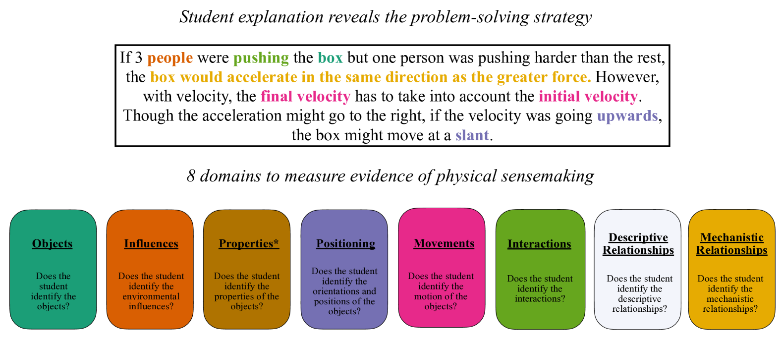
Figure 1: An annotated student explanation in response to Problem 4 (II.1) from Tufts’ Intro. to Physics course. We display the 8 domains used to classify words and phrases in the student’s text, where each domain can contain a different number of criteria to identify dependent on the problem. We color words and phrases that would prompt yes answers to the criteria questions within that same-colored domain. The descriptive relationship domain is colored light gray to represent that it is not relevant for the particular problem (i.e. the number of criteria is zero). The * next to the domain name signifies that the student failed to identify its criteria. More than one word or phrase can be annotated the same color if criteria multiplicities exist in that domain (e.g. positioning 1: “upwards” , positioning 2: “slant”). This particular student displays high evidence of physical sensemaking ($s=0.89$) by imagining a scenario where multiple interactions are influencing the boxes’ dynamics and communicating the resulting mechanistic relationship between a net external force and a change in the boxes’ motion.

II.2 Post-Hoc Measurement as Multi-Label Binary Annotation

Figure 1 demonstrates how an individual student explanation can be annotated with respect to 8 domains; however note that not all 8 domains are relevant (in Fig 1 the descriptive relationships domain is not relevant to the particular problem) and some domains occur multiple times (e.g. the object has more than one positioning in the context of the overall problem). As such, the full set of yes/no criteria questions across the 8 domains is problem-specific. Thus, for a set of $P$ problems, an annotator can follow the proposed steps:

Step 1. Select $P$ problems from a particular subject area (e.g. classical mechanics), where there exists a physical phenomena to be sensemade in each problem as a part of the strategy to solution.

Step 2. For each problem $p\in\{1,..,P\}$ and for each domain $d\in\{1,..,8\}$, determine the set of yes/no criteria questions $C^{p}_{d}$ that are pertinent to the specific problem. For example, in Problem 4 (II.1), there is only a single object and thus $|C^{4}_{1}|=1$ with the criteria question Does the student identify the object?. However, there are two positioning criteria questions $|C^{4}_{4}|=2$ that are relevant to sensemaking an object’s positioning under a net external influence: Does the student identify the object positioning before the net applied force? Does the student identify the object positioning after the net applied force? The annotator should end up with the total number of criteria questions per problem as $T_{p}=\sum_{d=1}^{8}|C^{p}_{d}|$.

Step 3. Given a student’s text response to problem $p$, the annotator will use the yes/no criteria questions to obtain a vector of binary digits representing their answers. The resulting criteria vector for a student response $n$ is denoted as $\textbf{y}^{n}\in\{0,1\}^{T_{p}}$. To further compute a sensemaking score $s\in[0,1]$ one can sum the number of $1s$ and divide by the length of the vector $T_{p}$. This score is to be interpreted as the amount of evidence of physical sensemaking. An annotator can also decide to weight the domains (or specific criteria) differently. In this work, we consider all domains and criteria to equally contribute to the sensemaking score. To finish off our example, the criteria vector for the student explanation in Fig. 1 is ${\textbf{y}}^{n}=[1,1,0,1,1,1,1,1,1]$ with the corresponding sensemaking score $0.89$. The student achieved such a high score by imagining a scenario where multiple interactions are influencing the boxes’ dynamics and communicating the resulting mechanistic relationship between a net external force and an the boxes’ change in motion. The student received a yes for all criteria except for the one in the property domain. The full list of criteria for Problem 4 is displayed in the Appendix A).

II.3 Theoretical Benefits and Limitations

Utility. This annotation scheme is intentionally designed to measure evidence of physical sensemaking given student explanations. The measurements allow for evidence of sensemaking to be quantitatively compared to other numerical values of interest, and distinguished from correctness. For example, evidence of sensemaking is different from measuring sensemaking correctness (i.e. the student is engaging in the sensemaking process with information that is determined by the authority figure to be canonically correct). The current scheme could be easily modified for this other purpose; the annotator would simply need to choose to annotate for both sensemaking and correctness according to the problem (e.g. the student identifies the correct positioning). However in this work, we stick to sensemaking scores that measure evidence of sensemaking, and leave correctness for future studies. Moreover, we emphasize that low sensemaking scores measured do not indicate that students cannot sensemake. It simply measures that in the current snapshot, evidence of sensemaking is low. There could be several reasons as to why the evidence is low (i.e. the problem itself didn’t encourage sensemaking, the student applied a memorized fact or procedure, etc.). Put concretely, our annotation scheme does not allow one to make any claims about causality.
Flexibility. Individuals can design or select their own problem sets, and then annotate the student explanations according to the same 8 domains. In proposing such an adaptive scheme, we attempt to balance imposing a systematic procedure with allowing the annotator to have enough freedom to make decisions.
Reproducibility. We provide a step-by-step outline of the annotation procedure, concise definitions of the 8 domains, and annotated examples of 385 student explanations across 4 physics problems of different criteria vector lengths. Our hope is that this content leaves little ambiguity for a new annotator looking to reproduce our results or implement the scheme in their own work. However, we acknowledge that some variability among annotators could exist and be quantified in the future with inter-rater reliability studies [39].
Reducibility. Each criteria vector length $T_{p}$ is the amount of binary information (bits) required to represent the evidence of a student’s sensemaking with respect to a particular problem. It is indeed possible that the 8 domains and criteria could be reduced such that a fewer number of binary variables are needed. While a reduced model form is not currently known; we speculate that such a form could exist.
Scalability. We acknowledge that manual annotation of a large number of student responses would require many hours of labor, often infeasible in practical settings. For example, the student explanation in Fig 1 took $\approx 3.8$ minutes to annotate. For a class of one-hundred students, this extrapolates to $\approx 6.3$ annotation hours with respect to a single problem. To resolve this scalability challenge, we show how the procedure can be automated by training an ML classification model on student explanations.

II.4 Sensemaking Related Works

Odden and Russ explicitly define sensemaking as “the dynamic process of building an explanation to resolve a perceived gap or conflict in knowledge.” The authors provide examples of individuals engaging in this process, and discuss how sensemaking can be conceptualized in three ways: a stance or framing (i.e. an individuals’ expectation of themselves in their current situation), a cognitive process built on the theory of knowledge integration, and a discourse practice related to argumentation. Each conception addresses what sensemaking is with respect to a different system level of study. Cognitive theories are based on the mental components and interactions happening during sensemaking, whereas framing can be considered one hierarchal level up as a latent description of a student’s current expectations in their environment when sensemaking is taking place. Lastly, discourse analysis is based on studying the content within and form of conversational dialogue between students.

Qualitative analysis has shaped our understanding of how sensemaking begins, functions, and ends for students. Odden and Russ [15] demonstrate how vexing questions stimulate the sensemaking process and can sustain it for longer durations of time than typically observed. Benedict-Chambers et al. [40] provides four specific types of questions focused on guiding students towards sensemaking including explication, explanation, science concept, and science practice questions. To characterize the explicit features of in-moment sensemaking, Odden and Russ [23] propose that the process be modeled as an epistemic game. This model introduces sensemaking as a three step procedure: 1. noticing a gap or inconsistency, 2. generating a mechanistic explanation, and 3. resolving the gap or inconsistency. The authors discuss a precursor to sensemaking, which includes assembling a knowledge framework by initially discussing ideas socially. This brainstorming step is necessary for one to eventually recognize a gap in their own knowledge system. During the game, the students can make moves (e.g. refining a question, appealing to reality, building an analogy, etc.) and if certain constraints are violated, students exit the game play. Three insightful constraints are discussed: 1. sensemaking is a discussion between individuals rather than an imbalanced monologue, 2. sensemaking occurs when there is a phenomena to sensemake that has not already been sensemade, and 3. sensemaking contains self-generated definitions of ideas alongside formal definitions. Kapon [20] puts forth a metric for how explanations generated during the sensemaking process are implicitly evaluated by individuals - based on intuitive knowledge, mechanism, and framing. More specifically, students evaluate explanations as “good enough” based on whether it aligns with their phenomenological experiences, is mechanistic rather than teleological, and satisfies their immediate expectations of their own understanding. Odden [19] explores how conceptual blends support sensemaking through a qualitative case study of students using concepts from kinematics to understand the mechanisms that underlie the phenomena in electric circuits. The author proposes the approach of generalizing conceptual ideas from one sub-area of physics to another as a mechanism that allows students to make connections in the sensemaking process. Furthermore, Sirnookar et al. [18] explores the role of modeling in sensemaking and analyzes the interactions of these two processes as two students are interviewed while solving a physics problem. The authors find that barriers in modeling can inhibit students’ sustained sensemaking.

In pursuit of the longer-term impacts of sensemaking, Radoff et al. [14] provides a qualitative account of a student engaging in sensemaking throughout an academic semester. Interviews and coursework demonstrated that experimentation with sensemaking caused more positive associations with learning, taking on challenges, and constructive confusion. In Kuo et al. [31], the authors show through a controlled classroom experiment that students who are instructed with mathematical sensemaking stimulation are prone to obtaining solutions to physics problems that are more accurate and insightful than those who did not receive this type of explicit instruction.

The sensemaking literature is fragmented across several scientific disciplines and is also typically broken into categories of scientific and mathematical sensemaking, where more recent work has attempted to define a blended model of the two [16, 26, 27]. Kaldaras and Wieman  [27] build upon prior works to put forth a cognitive model of blended math-science sensemaking that introduces three levels of sophistication: 1. developing qualitative relationships among relevant variables in mathematical equations that describe a particular phenomenon, 2. developing mathematical relationships among these variables, and 3. explaining how the mathematical operations used in the equation connect back to the physical phenomena. The authors attempt to validate their model by analyzing student responses from interviews, specifically probing the various levels of sophistication in the framework. While the authors found convincing evidence that the levels of sophistication were present across all student responses, it remained inconclusive as to whether there exists an actual sophistication ranking in the levels. As a result, it is still uncertain whether there exists a hierarchy among cognitive connections in math-science sensemaking. This work is directly linked with research that asks: what does it mean to understand a physics equation? [34] and seeks out structure in symbolic expressions that aid in student understanding.

The works above collectively agree on a key characteristic of the sensemaking process: the dynamic generation of mechanistic explanations for a given phenomena. When students have resolved their inconsistency, they have settled on a mechanistic explanation. The emphasis on mechanism in sensemaking is historically tied with research that characterizes student’s mechanistic reasoning in the classroom [17, 25, 41]. Russ et al. is arguably the the most influential contribution made thus far in defining mechanism in the context of STEM Ed., providing a framework for discourse analysis developed from ideas in philosophy of science [25]. In the framework, mechanistic reasoning is characterized as a process that uses experience-based evidence to construct causal relationships among objects describing “how underlying structure and activities can account for observable changes in a system”. The work puts forth a coding scheme of nine categories: 1. describing the target phenomenon they are trying to explain, 2. identifying setup conditions of the spatial and temporal organization of entities that construct the phenomena, 3. identifying the entities as components that construct the phenomena, 4. identifying activities (actions and interactions) of the entities, 5. identifying properties of entities, 6. identifying the spatial organization of entities relative to each other, 7. chaining reasoning strategy for backward or forward inference, 8. analogies, and 9. mental model animation. This framework has been widely adopted by the STEM Ed. community for qualitatively analyzing student reasoning, and we highlight that it overlaps significantly with our 8 domains presented to measure the evidence of sensemaking. There are a few key differences. The first is that we separate entities into objects and influences, where influences interact with objects in such a way that only the influence $\rightarrow$ object effect is relevant to the particular phenomena. This is especially useful when dealing with fields in physics, which are impacted from object interactions, but the effects are oftentimes ignored in classical settings or introductory courses. Our two domains positioning and movement track both the set-up and subsequent conditions of the dynamics of each object. The positioning domain also includes how the objects relate to one another structurally (i.e. object A is on top of object B) when this is relevant for the particular phenomena. As such, we reduce three of the codes (2,6,9) in Russ et al. to a single domain. As we aim to measure post-hoc explanations rather than in-moment discourse, we can code for the chaining and analogy creation process (which can be viewed as sub-sensemaking processes) proposed in Russ et al. by annotating whether the student identifies the relevant mechanistic relationships. In addition, we add a domain for descriptive relationships, which are the relations between the properties of objects - more akin to correlation than causal mechanism. Otherwise, with respect to Russ et al., our properties domain directly maps to code 5 and our interactions domain directly maps to code 4. As previously stated, our work builds off of the numerous qualitative studies discussed above that have identified the features of sensemaking and mechanistic reasoning through analyzing student discourse. We view our main contribution as transforming these features into 8 domains that contain sub-questions with binary outcomes such that we can obtain a post-hoc sensemaking measurement of a student’s explanation with respect to any particular physics problem. Introducing such a binary encoding scheme allows one to quantify evidence of student sensemaking and naturally lends itself to automating the measurement scheme with ML.

III How to Automate Measurements

III.1 Multi-Label Binary Classification Model

ML models have been shown to be capable of replacing labor-intensive encoding of qualitative data with automated procedures [41, 42, 43, 44, 45]. In this work, we only consider models which are open-access, which allows us to train classifiers for our specific task and does not require us to share student data with a 3rd party. Furthermore, we limit our consideration to models which are capable of running on consumer hardware. In our scenario, the task is the same as the human annotator’s: to map student text explanations across independent problems to sensemaking scores $s$.

From text to embeddings. Given a student explanation $n$, we can select an encoder to map all text in the response to a numerical representation $\textbf{x}^{n}$. A simple encoder design is counting; we determine a vocabulary $\mathcal{V}$ as the set of words across all student explanations in the training dataset, with an additional vocabulary entry for unknown words, and record the number of times each one appears in the $n^{th}$ example. This numerical representation, or embedding $\textbf{x}^{n}\in\mathbb{R}^{|\mathcal{V}|}$, typically called BagofWords, reduces the richness of the text explanation to the pattern of word occurrence [46, 47]. From here on, we will refer to this encoder as BoW.

Figure 2: How the proposed model makes a probabilistic prediction to answer a yes/no criteria question given a student explanation. Using a selected encoder, the student explanation is embedded into a numerical vector representation ${\textbf{x}}^{n}$. An embedded representation of the criteria context ${\textbf{q}}^{c}$ is added to ${\textbf{x}}^{n}$, producing an updated embedding ${\textbf{z}}_{c}^{n}$ contains information about both the student explanation $n$ and the current criteria question $c$. Finally, out of 8 possible domain-specific logistic regression classifiers, the current question’s domain $d$ selects its specific classifier to produce a predicted probability $\rho_{c,d}^{n}$ of answering “yes” to the criteria question. As a training objective, we use the cross-entropy loss comparing this probability to supervisory ground-truth label $y^{n}_{c,d}$. Each LR classifier’s weights and bias are updated via gradient-descent to minimize the sum of this loss over the entire training set. When using BERTfinetuned as the encoder, encoder parameters are also updated to minimize the loss.

To capture more complex patterns (e.g relative co-occurrence between all words in the explanation, in-context word occurrence, and word positional associations with grammar rules), one can use a large language model (LLM) encoder [48]. For example, Google’s BERT (Bi-directional Encoder Representations from Transformers) model combines tokenization, self-attention, and a multi-layer perceptron neural network - all pre-trained on English Wikipedia and BookCorpus to generate token embeddings [35]. A token is a set of characters containing a unique ID in BERT’s vocabulary, such that an entire text can be converted to tokens with individual embeddings $\textbf{x}^{n}_{token}\in\mathbb{R}^{768}$, which carry information about all other tokens in the sentence. BERT also uses a sentence-level embedding, known as $\textbf{x}^{n}_{CLS}\in\mathbb{R}^{768}$, which can be used as a full-response representation rather than using distinct representations for each token. From here on, we will refer to this encoder as BERTfrozen. Additionally, $\textbf{x}^{n}_{CLS}$ can be fine-tuned by training BERT’s previously trained weights $\{\bm{\theta}\}$ on new downstream classification tasks [49]. We will refer to this encoder as BERTfinetuned. While requiring more computational resources, this allows for the $\textbf{x}^{n}_{CLS}$ embedding to capture patterns in the text that are specific to the target prediction task.

Shared classifiers across problems. Given a generated embedding $\textbf{x}^{n}$ for a student explanation, we want to classify the representation into its correct criteria vector $\textbf{y}^{n}$. Thus, we have a multi-label task [50]. If we construct separate binary classification models for each criteria question, then we are required to train $T_{p}*P$ independent classifiers. Rather, we propose to work off of an informed assumption: shared domains will have similar word occurrence and grammatical structure across P problems. For example, the phrase “speeding up” should indicate evidence of sensemaking in the movement domain regardless of the problem it appears in , and words that should be classified as objects will share similar positions in the sentence across problems due to object-subject-verb rules. Thus, for $P$ problems, we can train 8 independent classifiers. We reduce from a scaling linear in $P$ to constant in $P$. Note that we are proposing to train 8 classifiers to obtain annotations for student explanations across problems, where each problem has a different number of criteria questions per domain $|C^{p}_{d}|$. Thus, to obtain an annotation for each criteria question within a domain, we add a criteria context embedding $\textbf{q}^{c}$ to each text embedding for a given student explanation. The updated embedding vector is denoted as $\textbf{z}^{n}_{c}$. The index $c\in\{1,..,|C^{p}_{d}|\}$ specifies the criteria question that we would like for the classifier to label (e.g. Does the student identify the object positioning before applied force (e.g. upwards)?). We note that there are multiple possible ways to encode this context. For example, rather than adding the vectors to obtain the updated embedding, one could concatenate the two vectors together. Additionally, one could embed the entire problem text alongside the specific criteria question. As a starting point, we’ve selected our approach of adding the embeddings together and only including the criteria question. We leave the exploration of alternative methods for future work.

Figure 2 visually illustrates how the model makes a probabilistic prediction answering a specific yes/no criteria question given a student-generated text response. Given embedding $\textbf{z}^{n}_{c,d}$, we use a domain-specific logistic regression (LR) classifier to produce the predicted probability $\rho^{n}_{c,d}\in(0,1)$. We set $\rho^{n}_{c,d}=\sigma(\textbf{W}_{d}\textbf{z}^{n}_{c,d}+b_{d})$, where $\textbf{W}_{d},b_{d}$ are the weight vector and bias scalar for domain $d$, and $\sigma$ denotes the logistic sigmoid function.

The figure also shows how that prediction impacts the loss used to train the model. For training, we have a dataset student embeddings with human annotated labels (the criteria vectors) $D_{\text{Train}}=\{\textbf{x}^{n},\textbf{y}^{n}\}_{n=1}^{N}$. Each $y^{n}_{c,d}\in\{0,1\}$ represents a single binary label with respect to criteria question $c$ of domain $d$ for the student explanation $n$. Each $y^{n}_{c,d}$ is assumed conditionally independent of other labels given $\textbf{x}^{n}$ and all model parameters.

We minimize the following binary cross entropy loss with an added regularization term over the weights averaged over all explanations, domains, and criteria:

$$\ell(\rho^{n}_{c,d},y^{n}_{c,d})=-(~y^{n}_{c,d}\log(\rho^{n}_{c,d})+(1-y^{n}_{c,d})\log(1-\rho^{n}_{c,d}))$$ (1)

For the precise loss notation utilized in our methods including regularization terms, see Appendix C. The training procedure encourages all 8 classifiers to accurately predict their assigned pieces of the criteria vector $\textbf{y}^{n}$ for an embedded student explanation $\textbf{x}^{n}$.

For some encoder choices, we do not update any encoder parameters during training; only the classifier weights and biases $\{\textbf{W}_{d},b_{d}\}_{d=1}^{D}$ are updated via gradient descent. When fine-tuning BERT, our gradient descent procedure updates encoder parameters $\{\bm{\theta}\}$ alongside classifier weights. Both are explored in our deployability analysis in IV.1.

III.2 Theoretical Benefits and Limitations

Utility. The proposed model maps new student text explanations across a set of problems to sensemaking scores $s$, freeing up time for an annotator. However, the current version of this model is limited to measuring sensemaking scores of student explanations on the same set of problems. We hypothesize that with more labeled training data across new problems, the model proposed here will have enough data to perform well on unseen problem instances in physics. However, the amount of data needed to cross such a threshold is unclear. Regardless, initial efforts to address this limitation should be directed towards collaborative annotation.
Reproducibility. The automation scheme ensures that the same student explanation receives the same annotation. The process is fully deterministic given fixed seeds to control for randomness. Randomness is only present in the initialization of the classifier weights and biases.
Sustainability. As ML research advances, new encoders may be able to improve the overall classification performance. However, many of these models require High Performance Computing (HPC) access and large amounts of energy resources for training [51]. As language modeling in ML improves, it is worth benchmarking new methods while also taking into account the amount of compute resources required to obtain only modestly better performance.

III.3 ML for Education Related Works

Machine learning tools are slowly integrating into STEM Ed. research methods, mostly with the introduction of text classification models [52, 43, 44, 45, 53]. One focus is on in-context learning, where student text responses are directly fed into a chatbot window of a large language model to be labeled [42]. This procedure can be conducted with a few examples (or zero) of student text, opening up an opportunity for non-ML practitioners to seamlessly use computation for data annotation. However, this procedure relies on the assumption that pre-trained language models are useful for specific tasks in education (e.g. classifying correctness, reasoning, sensemaking, etc.). Other works focus on training supervised ML models from scratch for their specific task [44, 45, 41]. For example, Watts et al.  [41] uses the mechanistic reasoning approach from Russ et al. to analyze student explanations in organic chemistry with the aid of ML binary classifiers. This work determines convolutional neural networks to outperform other model architectures for this task, but does not provide comparison results to other models. In our work, we provide a model comparison with three different language encoders (BoW, BERTfrozen, and BERTfinetuned), where we also fine-tune a pre-trained large language model on data for our specific task. Furthermore, we use a multi-label scheme that allows us to take advantage of shared structure across problems by providing each classifier with additional context for the problem-specific criteria we care about. As such, our classifiers are able to train on and classify new data across different physics problems without introducing new classification heads.

In response to the increasing amount of supervised ML models in STEM Ed. research, Fussell et al. [54] effectively summarizes and provides a demonstration of the best practices widely used by ML practitioners for validating these ML models. We note that our work utilizes methods advised by this work, including both cross-validation and bootstrapping. Lastly, we note that while our work does not fall under the category of unsupervised learning, these models are a promising avenue of research in STEM Ed. and can be used to cluster student data, detect static latent variables in student text, and analyze the latent dynamics within student conversations [55].

IV Practical Implementation Results

IV.1 ML Model Deployability Analysis

We seek to determine the deployability of the proposed classification models outlined in Sec. III.1. More specifically, our intention is to estimate how these models will perform given explanations from new students that it has never seen before, but on the same set of problems. Below, we outline our implementation and evaluation procedures prior to showcasing final results.

Figure 3: Model performance across sensemaking domains. For each domain, we show the average AUROC and 95% confidence interval from our 1000 bootstrapped test samples. Here, we see that BERTfrozen has the best performance in 2 domains (objects and mechanistic relationships), and BERTfinetuned has a higher average AUROC in the other 5 (other than properties). We observe that all 3 models are quite good at detecting evidence that a student has sensemade an object, but do worse on domains with less data. The properties domain only has 8 positive examples in the entire dataset, which were all used in training. As such, we are unable to report the AUROC for the properties domain.

Dataset of student explanations. Our dataset consists of 385 total de-identified student explanations across four problems distributed to students in the first few lectures of the 2023 Tufts University Introduction to Physics course. All problems have the same structure as Problem 4 II.1 shown above and are presented to the students as pre-lecture digital assignments [38]. The same $100$ students are asked to solve each problem and explain how they obtained their solution. A few students chose not to respond to a particular problem, which brings our total number of explanations to $385$. The problems capture different general core material for students to sensemake: (1) the descriptors of an object’s motion and dynamics; (2) the model of an object’s motion and dynamics under Earth’s gravitational influence; (3) the model of the relative motion of objects; (4) the model of an object’s motion dynamics under a net external influence. These problems vary in criteria vector size: $\{T_{1}=7,\ T_{2}=11,\ T_{3}=11,\ T_{4}=9\}$ (see Appendix A for exact problems and their details from [38]). The annotation procedure was carried out by a domain expert: the first author of this work who holds a doctorate in physics.

Model and training specifics. In our analysis, we use the following models BoW, BERTfrozen, and BERTfinetuned. To evaluate performance, we randomly select 15 students who responded to all four questions to use as a held-out test set and use the rest of the data for training and validation (325 samples). To prevent data leakage, we stratify the data by students to ensure that responses from the same student do not end up in both training and test/validation sets.

All models are trained with the Adam optimizer [56] for $1000$ epochs. We perform a grid search over key model hyperparameters: learning rate $\alpha$ and regularization strength $\lambda$ ($\lambda_{1}$ for classifier weights and $\lambda_{2}$ for BERT model weights), the full-details of which are available in Appendix D. For BoW and BERTfrozen, we use a 5-fold cross-validation approach for hyperparameter selection, where we select the hyperparameter combination with the best final average AUROC score across folds. AUROC is the computed area under a Receiver Operating Characteristic (ROC) curve defined by the true positive rate vs. the false positive rate of the predicted labels at different classification thresholds. There are two main reasons we believe AUROC to be the most useful metric for our context: (1) It does not require us to choose an arbitrary probability threshold to distinguish our positive predictions (label 1) from our negative predictions (label 0) for each classifier. Instead AUROC sums over all possible thresholds, providing a good summary that is still bounded, AUROC $\in(0,1)$, with increasing values indicating better performance. (2) Due to imbalanced annotations (i.e. some classifiers have more of a positive or negative class rather than a 50-50 split) in our training dataset, AUROC is a safer metric to report than precision or accuracy, as the chance baseline is $0.5$ independent of imbalance. We include an annotation summary of the data in the Appendix B.

The best model for BoW achieved an average AUROC score of $0.839$ across validation folds with the hyper-parameters: $\alpha=0.01,\lambda_{1}=0.001$. Similarly, for BERTfrozen, the best model achieved an AUROC score of $0.890$ with the hyper-parameters: $\alpha=0.001,\lambda_{1}=0.001$. For BERTfinetuned, we require a larger amount of computational resources per experiment, so we only used a single training and validation set to run the hyperparameter grid search. Note that we use an L2SP loss [57, 58] when training BERTfinetuned, consisting of two separate weight decay terms such that we can regularize the weights from the BERT encoder separately from the weights of our LR classifiers. This is done to best preserve the prior information learned in in BERT’s original training. We set the batch-size to $N_{batch}=32$, which has been shown empirically to work well with deep neural networks [59]. Overall, we run 324 fine-tuning experiments for BERTfinetuned on Tufts’ HPC services. We picked the model with the optimal final AUROC of $0.916$ on the validation set, which had the following hyperparameters: $\alpha=1e-5$, $\lambda_{1}=0.0001$, and $\lambda_{2}=0.1$.

Model evaluations. We retrain our selected models on all training and validation data, and evaluate on the held-out test set of $15$ randomly selected students (60 student explanations). To approximate uncertainty on unseen student explanations, we bootstrap our test set with replacement to generate $1000$ individual test sets for evaluating performance [60, 61]. In Figure 3, we show the average AUROC across independent test predictions for each of the 8 domain classifiers and for each model type. We are not able to report the AUROC for the properties domain as the class imbalance is extremely large and no positive examples were included in the test set. As such, we also provide the Area Under the Precision-Recall curve (AUPRC) results in Appendix E for all domain classifiers. This metric emphasizes the precision of the classifier, which informs us as to how well the model predicts the true positive labels. We note that even with AUPRC, there is too much uncertainty to make concrete claims about the deployability of the properties domain classifier. More positive data examples are necessary for improvement. We show the average AUROC across independent test set predictions for each model in Table 1. These values represent the annotation quality of our entire model. In Table 1, we also report the time taken to train the final selected model. To show the significance in results between models, we provide the $95\%$ confidence interval in Table 1 that results from our bootstrapping procedure and taking the AUROC differences between models. These values can be interpreted as the uncertainty intervals in AUROC difference across models, such that as long as zero is outside of the interval, we can be $95\%$ confident that there exists some non-zero difference between our models indicating that one is indeed better than the other. Additionally, we report the confusion matrices in Appendix F. BoW performs surprisingly well with an AUROC score of $0.839$ and trains efficiently in 1 minute. It performs nearly as well for objects as the other two models. This behavior is unsurprising as BoW reduces text to word frequency counts. BERTfrozen performs slightly better with an AUROC score of $0.890$ and takes 7 minutes to train. It performs the best for two of the domains: objects and mechanistic relationships. It is able to reliably outperform BoW on average, as 0 in not inside of the confidence interval between the AUROC classifier difference reported in Table 1. BERTfinetuned achieves an AUROC score of $0.916$. It takes 160 minutes to train, but we emphasize that this is not a prohibitive cost for a model which only needs to be trained when new student data is available. It performs the best for influences, positioning, movements, interactions, and descriptive relationships. It is able to perform the best overall despite only leading in 5 domains due to the imbalance in the occurrence of each domain. We recommend the BERTfinetuned model as we believe the average increase in performance across domains is worth the nearly 3 hour training time, and the confidence intervals in 1 indicate it is a significant improvement over BERTfrozen. However, if the annotator wants to optimize for a particular domain, they should refer to Figure 3 to decide the best model for their purpose.

	AUROC (95% CI)	Runtime
BoW	0.839 (0.803, 0.873)	1 min
BERTfrozen	0.890 (0.864, 0.915)	7 min
BERTfinetuned	0.916 (0.893, 0.939)	160 min

	Avg. (95% CI)
$\Delta\text{AUROC}_{\texttt{Finetuned}-\texttt{Frozen}}$	0.026 (0.005, 0.045)
$\Delta\text{AUROC}_{\texttt{Finetuned}-\texttt{BoW}}$	0.077 (0.051, 0.104)
$\Delta\text{AUROC}_{\texttt{Frozen}-\texttt{BoW}}$	0.051 (0.024, 0.079)

Table 1: Avg. model performance and comparison.

IV.2 Student Performance Analysis

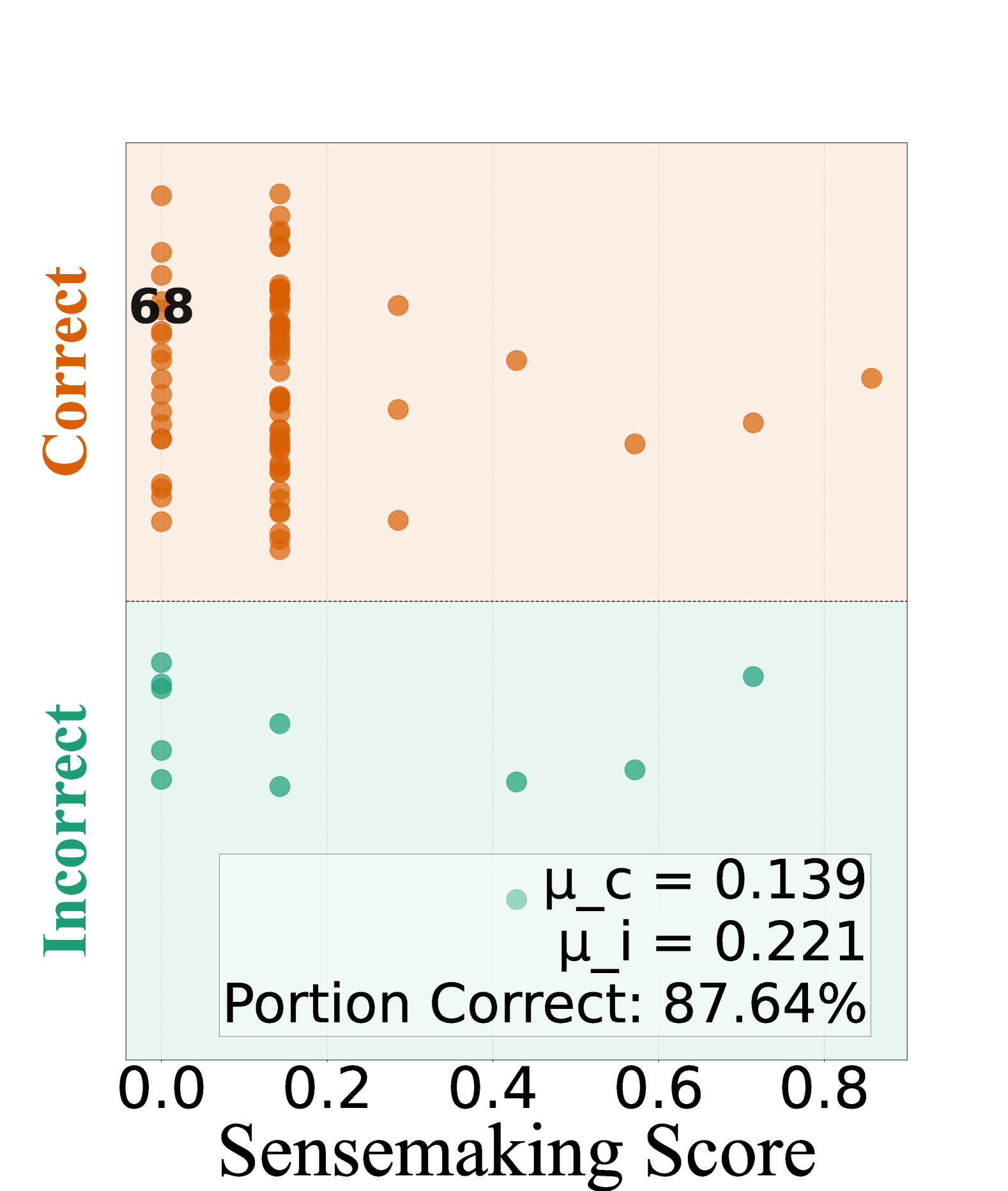
(a) Problem 1

(b) Problem 2

(c) Problem 3

(d) Problem 4

Figure 4: Student performance in Tufts Intro to Physics course. On four separate problems, we show the sensemaking scores $s$ of students alongside their binary correctness. We identify student $68$ to highlight how the measurements can be used to track sensemaking growth over time for a particular student. Here, sensemaking growth does not coincide with consistent correctness. The combination of the two variables provides a more nuanced picture of the student’s performance. In each problem, the relationship between the two variables appears different for the student popoulation: (a) high accuracies with low sensemaking scores, (b) high accuracies with varied sensemaking scores, (c) varied accuracies with high sensemaking scores, (d) varied accuracies with varied sensemaking scores. In summary, the results indicate that problem-solving accuracy is not a useful proxy for measuring evidence of physical sensemaking, nor vice versa.

We provide a quantitative snapshot of student performance in the first few weeks of the 2023 Tufts Intro. to Physics course. More specifically, we compute the sensemaking scores of students from their explanations to four problems (used in Sec. IV.1 and displayed in Appendix Sec. A), and compare these scores alongside problem-solving accuracies. Students reported their multiple-choice answer, such that accuracy here is a binary variable $a\in\{correct,incorrect\}$. Our results in Fig 4 show that assessing sensemaking scores provides a more nuanced view of student performance than correctness alone. In problem 1, we observe a high proportion of students solving the problem correctly ($87\%$) with very low sensemaking scores among correct answers ($\mu_{c}=0.139$). In problem 2, we also observe high correctness ($97\%$), but with higher sensemaking scores (an average of $\mu_{c}=0.472$) among correct answers. In these problems we observe students who obtain a correct answer with both high and low evidence of sensemaking. In fact, a closer look at the data reveals that many of these students who arrived at the correct answer without showing evidence of physical sensemaking deployed a learned mathematical rule (i.e. the derivative of velocity is acceleration).

In problems 3 and 4, we observe less correct answers across students ($71\%$ and $67\%$ respectively); however sensemaking scores remain high among both correct (average sensemaking scores of $\mu_{c}=0.607$ and $\mu_{c}=0.357$ respectively) and incorrect ($\mu_{i}=0.458$ and $\mu_{i}=0.479$ respectively) responses. Specifically in problem 4, the mean sensemaking scores for the incorrect group are higher than for the correct group. Recall that our measurement scheme determines evidence of the sensemaking process, not whether students have accurate information in the sensemaking process. Also, sensemaking has been characterized as a non-linear process to organize information that includes integrating ones phenomenological experiences, which often leads to constructive confusion [13, 14, 15, 16, 17]. Investigating the student responses reveals that students with higher sensemaking scores who arrived at the incorrect answer either used incorrect information or were unable to successfully make connections to their personal experiences with everyday physical objects.

Problem	$r_{pb}$	$95\%$ CI
1	-0.166	(-0.461, 0.145)
2	0.053	(-0.055, 0.176)
3	0.404	(0.227, 0.546)
4	-0.198	(-0.391, 0.009)

Table 2: The Point-Biserial correlation for each physics problem.

We show the Point-Biserial correlation coefficient $r_{pb}$, known as the binary-continuous form of the Pearson correlation coefficient $r$), for the student data in Table 2. The coefficient $r_{pb}\in\{-1,1\}$, where values farther from zero signals a stronger linear relationship and the sign indicates the direction. Only results in problem 3 suggest that there exists a positive linear correlation between problem-solving accuracy and sensemaking score; however, the coefficient is closer to zero than one indicating that the relationship strength is weak ($r_{pb}=0.404$). As we cannot assume normality in the underlying distributions over sensemaking scores for each binary group, we circumvent a hypothesis test with a bootstrapping procedure. We sample our data with replacement $1000$ times and generate an empirical distribution over $r_{pb}$ scores for each sample. We report the $95\%$ confidence interval in Table 2. All values within each interval remain closer to zero than $\pm 1$, except for problem 3 for the tail end of the confidence interval. The weak correlation present makes a clear point: problem-solving accuracy is not a useful proxy for measuring evidence of physical sensemaking, nor vice versa. If one were to only look at the accuracy scores, one might believe that students are learning the core material. Sensemaking scores add more nuance to this belief, suggesting that students are engaging in alternative methods to obtaining a problem solution.

There are multiple actions one could take to further analyze these measurements and use them in a practical context, especially at the individual student level. For example, measurements could be used to observe whether evidence of sensemaking for a particular student is declining, stable, or growing across problems in time. To show an example of this, we show the trend for student $68$ in Fig. 4. This student shows evidence of stable sensemaking growth, which does not always coincide with correctness. In fact, if one only observed the accuracy score, the student’s performance would appear to be declining. When both of these measures are combined, one observes a more nuanced picture of the student’s progress, which could lead to more informed interventions.

V Conclusion & Future Work

In this work, we contribute a post-hoc measurement scheme to quantify evidence of physical sensemaking via human annotation of student explanations to physics problems. To streamline the lengthy process of annotating each student explanation, we automate the measurement scheme with a trained ML model using language encoders and shared probabilistic classifiers. We implement three model variants with different language encoders and conduct a deployability analysis on real student explanations from Tufts’ 2023 Intro. to Physics course. We show that the ML models have good average performance on data from new students (0.916 AUROC for the best model), but performance is dramatically different across domains. Moreover, we show that across problems, we can now systematically measure evidence of student learning separately from problem-solving accuracy. In fact, we observe no linear correlation between these two variables. Such a result has important implications for both practical instruction and STEM Ed. research. First and foremost it suggests that we need to be more cautious with how we measure learning. It’s not always useful to make assumptions about the process from the outcome. Students obtaining correct answers does not necessarily indicate a student has engaged in physical sensemaking, as there are alternative strategies, oftentimes requiring less time in the short-term, to achieve the same goal. As previous works support, sensemaking can more directly be measured by paying attention to how students solve problems - whether that’s through a post-hoc written explanation or an in-moment oral discussion. The former is where we’ve focused our efforts, but we believe the latter can also be more efficiently executed with ML tools. Beyond this, we perceive two next-stage research questions that lie at the intersection of ML and STEM Ed. fields:

(1) How can this post-hoc measurement scheme be improved? On the ML side, a natural first reaction is more data. We hypothesize that with more labeled training data across new problems, the models proposed here will be able to achieve better performance on the current task and generalize to unseen problems. Given collaborative annotation efforts, such a model could be realized more efficiently and would save all users time in the long run. We invite interested collaborators to get in touch and encourage open sharing of sensemaking data when possible and appropriate. One could also experiment with new state-of-the-art encoders to enhance overall performance [62]. For example, using the Mistral model (open access, open source transformer model in Ref. [63]) as the LLM text encoder, pre-trained with 7 billion parameters and 2 million language tokens. As off-the-shelf language models improve, one might not need as much training data to obtain quality performance. Lastly, our ML model assumes domain independence in the classification task. Perhaps there is a shared structure across domains that could be exploited. As a brief intuitive example, consider the perspective of an annotator. Given that the annotator identifies criteria in the first two domains (objects and influences), it is more probable that the annotator will identify criteria in the other domains. On the STEM Ed. side, we need to better understand how we can design problems that are aligned with the measurement scheme without creating a new performance metric for students. We do not want the annotation criterion to be perceived by students as tasks to complete. This runs the risk of students inventing alternative strategies to effectively mimic sensemaking. An example of this would be pattern recognizing the types of explanations that lead to high sensemaking scores. As shown by our ML model, this isn’t a very difficult task. Ideally, we prompt students to sensemake and our measurement scheme does not disturb their epistemic framing. There exists an open research pursuit in STEM Ed. to understand how problems can be effectively designed and communicated to students such that genuine sensemaking is encouraged [40].

(2) How can we model the dynamics that lead to low vs. high evidence of physical sensemaking in the classroom? Our proposed measurement scheme only provides evidence of a student’s sensemaking at a single point in time. We lack a model as to how students evolve such that specific sensemaking scores are realized. It is of high interest to construct both deterministic and probabilistic ML mechanistic models that capture short and long-term developmental dynamics of student sensemaking in physics classrooms[64, 65].

Appendix A Physics Problems & Annotations

We provide all four physics problems as they originally appeared to students from Ref. [38]. For each problem, we show the specific annotation scheme - i.e. the specific criteria questions for each problem.

Problem 1 1. Which plot best represents the acceleration curve associated with the displacement and velocity curves shown here? 2. Briefly explain your answer to the previous question. Annotation Procedure 1 Components (1) Does the student identify the object (object, car, etc.)? Characteristics (2) Does the student identify the orientation (e.g. left or right)? (3) Does the student identify movement 1 (e.g. slow down)? (4) Does the student identify movement 2 (e.g. zero)? (5) Does the student identify movement 3 (e.g. speed up)? Relationships (6) Does the student identify the descriptive relationship (e.g position changes is a pos/neg velocity)? (7) Does the student identify the descriptive relationship (e.g velocity changes is a pos/neg acceleration)?

Problem 2 A physics demo launches a ball horizontally while dropping a second ball vertically at exactly the same time. 1. Which ball hits the ground first? (a) Dropped ball (b) Launched (horizontally) ball (c) Both hit at the same time 2. Briefly explain your answer to the previous question. Annotation Procedure 2 Components (1) Does the student identify object 1 (e.g. ball 1)? (2) Does the student identify object 2 (e.g. ball 2)? (3) Does the student identify the possible environmental influences on object 1 (e.g. gravity)? (4) Does the student identify the possible environmental influences on object 2 (e.g. gravity)? Characteristics (5) Does the student identify object 1 positioning (e.g. down)? (6) Does the student identify object 2 positioning (e.g. horizontal up)? (7) Does the student identify object 1 motion (e.g. speeding up)? (8) Does the student identify object 2 motion (e.g. speeding up)? Relationships (9) Does the student identify the interaction between object 1 and gravity (e.g. gravitational force)? (10) Does the student identify the interaction between object 2 and gravity (e.g. gravitational force)? (11) Does the student identify the mechanistic relationship between gravity and a change in motion (e.g. Earth’s gravitational force is a mechanism that causes the object to move down at a constantly increasing speed)?

Problem 3 A girls stands on a moving sidewalk (conveyor belt) that is moving to the right at a speed of 2 m/s relative to the ground. A dog runs on the belt toward the girl at a speed of 8 m/s/ relative to the belt. 1. What is the speed of the dog relative to the girl? (a) 10 m/s (b) 6 m/s (c) 8 m/s Annotation Procedure 3 Components (1) Does the student identify object 1 (e.g. girl)? (2) Does the student identify object 2 (e.g. dog)? (3) Does the student identify object 3 (e.g. moving sidewalk, conveyor belt)? Characteristics (4) Does the student identify the positioning of the dog (e.g. left)? (5) Does the student identify the positioning of the belt (e.g. right)? (6) Does the student identify the movement of the girl (e.g. at rest)? (7) Does the student identify the movement of the dog (e.g. 8m/s constant speed)? (8) Does the student identify the movement of the belt (e.g. 2 m/s constant speed)? Relationships (9) Does the student identify the interaction between the girl and the belt (e.g. moving her to the right)? (10) Does the student identify the interaction between the dog and the belt (e.g moving the dog to the right)? (11) Does the student identify the mechanistic relationship between motion of the observer and motion of the observed? (e.g. the speed of the observer relative to the observed object in motion causes the observed motion)

Problem 4 1. The net force on the box is in the positive x direction. Which of the following statements best describes the motion of the box? (a) Its acceleration is parallel to the x axis. (b) Its velocity is parallel to the x axis. (c) Both its velocity and acceleration are parallel to the x axis. (d) Neither its velocity not its acceleration need to be parallel to the x axis. Annotation Procedure 4 Components (1) Does the student identify the object (e.g. object, box, etc.)? (2) Does the student identify the possible environmental influence acting on the object (e.g. applied net force)? Characteristics (3) Does the student identify the object properties (e.g. mass)? (4) Does the student identify the object positioning before applied force (e.g. upwards)? (5) Does the student identify the object positioning after applied force (e.g. horizontal)? (6) Does the student identify the object movement prior to the applied force (e.g. constant velocity)? (7) Does the student identify the object movement after the applied force (e.g. final velocity)? Relationships (8) Does the student identify the interaction between the object and the net applied force (e.g. change in direction)? (9) Does the student identify the mechanistic relationship between an applied net force and a change in motion? (e.g. a net force applied in the x direction will be a mechanism that causes a change in motion/acceleration in the x direction)

Appendix B Annotation Tables

We provide an annotation summary. We showcase the number of student explanations per problem, and the number of those explanations being labeled as positive for each specific criteria.

Problem	Number of Responses
1	89
2	98
3	100
4	98

Table 3: The number of student explanations per problem.

Criteria#	Problem 1	Problem 2	Problem 3	Problem 4
1	9	89	97	66
2	4	89	96	62
3	6	49	78	8
4	1	48	36	21
5	4	40	9	46
6	6	40	80	20
7	63	46	92	44
8		46	29	41
9		21	54	42
10		20	36
11		18	13

Table 4: The number of positive criteria labels per problem.

Appendix C Loss Function Definition

Given the training dataset $D_{\text{Train}}=\{\textbf{x}^{n},\textbf{y}^{n}\}_{n=1}^{N}$ of assumed independent student embeddings with human annotated labels, we train all parameters $\Theta$ to minimize the following loss function:

$$\mathcal{L}(\Theta) =\mathcal{L}^{\text{BCE}}(\Theta)+\mathcal{R}(\Theta),$$ (2)

$$\mathcal{L}^{\text{BCE}}(\Theta) =\sum_{p=1}^{P}\sum_{i=1}^{N_{p}}\sum_{d=1}^{D=8}\sum_{c\in C^{p}_{d}}\frac{\ell^{i,p}_{c,d}}{DPN_{p}\max(1,|C^{p}_{d}|)},$$

$$\ell^{i,p}_{c,d} =-y^{i,p}_{c,d}\log(\rho^{i,p}_{c,d})-(1-y^{i,p}_{c,d})\log(1-\rho^{i,p}_{c,d}).$$

Here, $P$ is the total number of problems, $N_{p}$ is the total number of student explanations per problem in the dataset $D_{\text{Train}}$, $D=8$ is the total number of domains, and $C^{p}_{d}$ is the set of all context criteria (indexed by $c$) in a particular domain $d$ for a specific problem $p$. In the binary cross-entropy expression, $y^{i,p}_{c,d}$ is the ground truth prediction for the $i^{th}$ student explanation associated with problem $p$ with respect to domain $d$ and specific criteria $c$. $\rho^{i,p}_{c,d}$ is the corresponding predictive probability.

The loss representing fit to the training data is averaged over all examples. The overall loss also includes a regularization term $\mathcal{R}(\Theta)$ over all weights. When we train BERTfinetuned, we have both a regularization term in the loss for classifier weights $\{\textbf{W}_{d},b_{d}\}_{d=1}^{D}$ and the encoder weights of BERT $\{\bm{\theta}\}$. We use an L2SP loss [57, 58], which encourages weights for the LR classifiers to be close to zero, while encouraging BERT encoder parameters to be near pretrained values.

Appendix D Hyper-parameter Strategy

We outline our hyper-parameter procedure step by step such that the experiments in this work can be reproduced. For all experiments, we set the following seeds to control for randomness: $123$ when splitting the data, $360$ when running experiments with SGD, and $126$ when bootstrapping test sets.

BoW & BERTfrozen. We randomly select $15$ students for our held-out test set ($60$ explanations) and use the rest of the data for a randomized 5-fold cross-validation procedure, where we stratify by student ID. The student ID stratification is to ensure that there is no data leakage between students at train and test time - i.e. we don’t want the model learning student-specific correlations. As such, we ensure that all responses from a specific student are in the same fold. All splits are located in our Github Repo “AuSeM”.

We perform a grid hyper-parameter search while optimizing for the AUROC score over the following: learning rates $\alpha=\{0.1,0.01,0.001,0.0001,0.00001,0.000005,0.000001\}$, and weight decays $\lambda_{1}=\{0.1,0.01,0.001,0.0001,1e-5,0\}$. We average the value of AUROC from the last epoch from all 5 folds and pick the hyperparameter combination with the best AUROC score. The best model for BoW achieved an AUROC score of $0.875$ with the hyper-parameters: $\alpha=0.01,\lambda_{1}=0.001$. Similarly, for BERTfrozen, the best model achieved an AUROC score of $0.880$ with the hyper-parameters: $\alpha=0.001,\lambda_{1}=0.0001$.

BERTfinetuned. We use the same held-out test set, but instead of conducting a cross-validation procedure which is computationally expensive for fine tuning, we use the rest of the data as a train/val set for the hyper-parameter selection. The train/val set are also stratified by student ID. The split is located in our Github Repo. “AuSeM”.

We run a hyper-parameter grid search with an SGD optimizer for $1000$ epochs and batch-size to $N=32$ over the following: learning rate $\alpha=\{0.1,0.01,0.001,0.0001,0.00001,0.000001,0.0000005,1e-7,1,1e-8\}$, classifier weight decay $\lambda_{1}=\{0,0.1,0.01,0.001,0.0001,0.00001\}$, and BERT encoder weight decay $\lambda_{2}=\{0,0.1,0.01,0.001,0.0001,0.00001\}$. We use two weight decay variables such that we can regularize the weights from BERT separately from the weights of our LR, as we want to best preserve the information learned in the pre-trained model [57, 58]. This totals to 324 fine-tuning experiments for BERTfinetuned on Tufts’ HPC services.

We sort all models by optimal final validation AUROC and select the model that achieves the highest final AUROC $=0.946$. We observe that the model’s behavior appears stable. This model’s hyperparameters are: $\alpha=1e-05$, $\lambda_{1}=0.0001$, and $\lambda_{2}=0.1$. Note that prior to sorting by final AUROC, we sorted by $\max$ AUROC to determine whether a reasonable early stopping point could be identified. While some models did have higher intermediate validation AUROC values, this was only the case for unstable models with too-high learning rates. As such, we determined them to be unreliable, and did not find a place where early stopping would be useful.

Appendix E AUPRC Scores

We show the AUPRC scores for each independent classifier in Fig. 5 and the average AUPRC scores across models in Table 5.

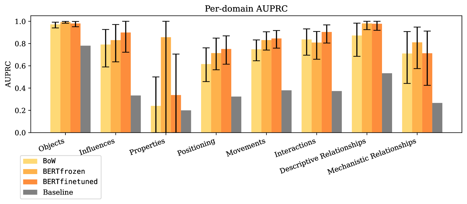
Figure 5: AUPRC model performance across sensemaking domains. For each domain, we show the average AUPRC and 95% confidence interval from our 1000 bootstrapped test samples. Here, we see that BERTfrozen has the best performance in 4 domains (objects, properties, descriptive and mechanistic relationships), and BERTfinetuned has a higher average AUPRC in the other 4 domains. We observe that all 3 models struggle in domains where there is limited data, especially in the properties domain where zero lies in the $95\%$ confidence interval. In grey we show the Baseline AUPRC value, the fraction of positive examples.

	AUPRC (95% CI)	Runtime
BoW	0.831 (0.788, 0.870)	1 min
BERTfrozen	0.881 (0.846, 0.911)	7 min
BERTfinetuned	0.896 (0.863, 0.927)	160 min

Table 5: Avg. model performance and comparison.

Appendix F Confusion Matrices

We present confusion matrices for all three methods. To produce binary predictions, we threshold the predicted probability at a value of 0.5. We observe similar performance here as in the AUROC scores (which take all possible thresholds into account). BERTfinetune has the fewest classification errors overall. However, we see that BERTfrozen makes slightly fewer false positive mistakes (45 compared to 47). For cases where one type of error has a larger cost than another, careful model and threshold selection are important.

BoW

$$\begin{array}[]{c|cc}\text{Actual}\backslash\text{Predicted}&0&1\\ \hline\cr 0&261&62\\ 1&70&177\end{array}$$

BERTfrozen

$$\begin{array}[]{c|cc}\text{Actual}\backslash\text{Predicted}&0&1\\ \hline\cr 0&278&45\\ 1&67&180\end{array}$$

BERTfinetuned

$$\begin{array}[]{c|cc}\text{Actual}\backslash\text{Predicted}&0&1\\ \hline\cr 0&276&47\\ 1&42&205\end{array}$$