Euclid Quick Data Release (Q1)

The Euclid space mission aims to investigate the nature of dark energy and dark matter by mapping the large-scale structure of the Universe. A key component of Euclid’s observational strategy is slitless spectroscopy, conducted using the Near Infrared Spectrometer and Photometer (NISP). This technique enables the acquisition of large-scale spectroscopic data without the need for targeted apertures, allowing precise redshift measurements for millions of galaxies. These data are essential for Euclid’s core science objectives, including the study of cosmic acceleration and the evolution of galaxy clustering, as well as enabling many non-cosmological investigations. This study presents the SIR processing function (PF), which is responsible for processing slitless spectroscopic data from Euclid’s NISP instrument. The objective is to generate science-grade fully-calibrated one-dimensional spectra, ensuring high-quality spectroscopic data for cosmological or astrophysical analyses. The processing function relies on a source catalogue generated from photometric data, effectively corrects detector effects, subtracts cross-contaminations, minimizes self-contamination, calibrates wavelength and flux, and produces reliable spectra for later scientific use. The first Quick Data Release (Q1) of Euclid’s spectroscopic data provides approximately three million validated spectra for sources observed in the red-grism mode from a selected portion of the Euclid Wide Survey. We find that wavelength accuracy and measured resolving power are within requirements, thanks to the excellent optical quality of the instrument. The SIR PF represents a significant step in processing slitless spectroscopic data for the Euclid mission. As the survey progresses, continued refinements and additional features will enhance its capabilities, supporting high-precision cosmological and astrophysical measurements.

1 Introduction

Slitless spectroscopy, also known as dispersed imaging, is one of the two operating modes of the Near Infrared Spectrometer and Photometer (NISP, Euclid Collaboration: Jahnke et al. 2024), one of the two instruments, along with VIS (Euclid Collaboration: Cropper et al. 2024), on board Euclid (Euclid Collaboration: Mellier et al. 2024). This high multiplexing spectrographic technique allows for the simultaneous dispersion of light from all sources within a given field of view, eliminating the need for traditional targeted apertures or slits, thereby enabling efficient spectroscopic measurements across vast regions of the sky.

The spectroscopic exposures captured by the NISP spectrometer (hereafter NISP-S) undergo comprehensive processing to generate scientifically valuable, decontaminated, wavelength- and flux-calibrated, combined one-dimensional (1D) spectra. This processing is handled by the SIR processing function (PF) within the Euclid science ground segment (SGS). The SIR PF produces spectra for all entries listed in the source catalogue independently produced by the MER PF (Euclid Collaboration: Romelli et al. 2025) from photometric data from Euclid visible (VIS PF, Euclid Collaboration: McCracken et al. 2025) and near-infrared (NIR PF, Euclid Collaboration: Polenta et al. 2025) observations, as well as selected external observations (EXT PF). The calibrated and validated spectra are subsequently passed to the SPE PF (Euclid Collaboration: Le Brun et al. 2025) for advanced spectral analyses, such as redshift determination and other spectral feature extractions. The SIR PF processes exposures from the NISP-S instrument, covering both wide and deep acquisitions, as well as red (‘RGS’, with passband ${\rm RG}_{\scriptscriptstyle\rm E}\approx\text{$12001900\text{\,}\mathrm{n}\mathrm{m}$}$ and resolving power $\mathcal{R}>480$) and blue (‘BGS’, with passband ${\rm BG}_{\scriptscriptstyle\rm E}\approx\text{$9201370\text{\,}\mathrm{n}\mathrm{m}$}$ and resolving power $\mathcal{R}>400$) grisms, although the Q1 release focuses only on red-grism data from the Euclid Wide Survey (EWS, Euclid Collaboration: Aussel et al. 2025).

During the Euclid Wide Survey (EWS), the reference observing sequence (ROS) plays a crucial role in structuring the observations (Euclid Collaboration: Scaramella et al. 2022). It is executed at every pointing, and consists of four dithers, where NISP-S and VIS observe simultaneously. Each dither involves a spectroscopic exposure with 549.6 s of integration time, covering approximately the same sky portion but with a distinct combination of red grism (RGS000 or RGS180) and grism-wheel assembly (GWA) tilt ($$$,\pm$$$), following the dithering ‘K’ sequence: RGS000+0 $\to$ RGS180+4 $\to$ RGS000-4 $\to$ RGS180+0. Consequently, each source will be observed approximately four times (except if they unfortuitously fall on detector gaps or field edges), providing as many ‘single-dither’ spectra.

In spectroscopy, it is important to distinguish between two key concepts, ‘spectrogram’ and ‘spectrum’, the counterparts of photometric concepts of observed image (2D) and inferred integrated flux (scalar).

In slitless spectroscopy, a spectrogram specifically refers to the observed two-dimensional trace of dispersed light on the detector, representing the source’s spectral content as a function of both spatial position and wavelength. By the design of the NISP instrument, SIR focuses on the trace of the first dispersion order of the grism (hereafter ‘1st-order spectrogram’), but such traces also exist for other dispersion orders (e.g., the 0th-order spectrogram).

In contrast, a spectrum refers to the one-dimensional spectrum of a source, representing its chromatic flux density independently of the dispersion order. The SIR PF will infer this ‘intrinsic’ spectrum from the 1st-order spectrogram under the ‘spectral separability’ hypothesis, which posits that the light distribution in both spatial and spectral directions can be factored into independent components: $C(x,y,\lambda)=I(x,y)\,S(\lambda)$, where $I(x,y)$ represents the spatial intensity distribution, and $S(\lambda)$ represents the spectral flux distribution. This assumption is valid for unresolved sources or spatially-resolved uniform sources. However, this hypothesis neglects potential spatial gradients in colour, internal flux distribution, or internal kinematics, which would require full-forward modelling of the spectrograms (Outini & Copin 2020).

While slitless spectroscopy offers significant advantages in efficiency and sky coverage, it is also susceptible to two major sources of contamination: ‘cross-contamination’, where the spectrograms of neighbouring sources (in the first or other dispersion orders) may overlap with the target source’s spectrogram, and ‘self-contamination’, which arises from the degeneracy of the spatial and spectral dimensions along the dispersion direction and which leads to an effective resolving power function of source spatial extent. The SIR PF mitigates these contaminations with sophisticated decontamination and virtual-slit techniques (see below), but these issues, still active fields of research, are not discussed further here.

This paper provides an overview of the SIR PF at the time of the data production (November 2024) for the Euclid Q1 release (Euclid Quick Release Q1 2025). It is organised as follows. Section 2 describes the individual processing steps that progressively transform raw slitless spectroscopic data into precise, calibrated spectra, including scientific (Sect. 2.3), calibration (Sect. 2.4), and validation and data quality control (Sect. 2.5) pipelines. Section 3 presents validation of the spectroscopic performance of the SIR PF in the light of the Euclid’s top-level mission requirements, and Sect. 4 concludes. All magnitudes are in the AB mag system (Euclid Collaboration: Schirmer et al. 2022).

2 Spectroscopic calibration and measurements

2.1 Overview

The SIR PF is split into three sets of pipelines, each of which contains individual processing elements that will be described in their respective sections. In addition to the main ‘scientific’ and ‘calibration’ pipelines (described below), a third ‘validation’ pipeline runs independently on a control field to assess and validate the software quality (Sect. 2.5).

2.1.1 The scientific pipelines

There are two independent scientific pipelines (Sect. 2.3), which are run sequentially for the processing of all scientific exposures acquired by NISP-S during the survey. Their objectives is to produce science-grade products, internal to SIR PF or for general publication, based on some pre-computed and validated calibration products.

The Spectra Extraction pipeline

delivers single-dither calibrated spectra; it runs sequentially on an observation basis during the processing of the scientific exposures. It includes the following eight science-related PEs.

Preprocessing:

identification and correction of NISP detector artefacts (e.g., dark current, nonlinearity, persistence, etc.). This step is common to the NIR PF (Euclid Collaboration: Polenta et al. 2025), since the same detectors are used both for photometry and slitless spectroscopy, although in different readout modes (Sect. 2.3.2).

Spectra location:

full mapping between the sky coordinates of an arbitrary source and the precise position of the corresponding spectrograms in the focal plane (FP) as a function of wavelength and dispersion orders (Sect. 2.3.3).

Detector scaling:

estimate of the incident spectrum on each pixel (scene model) and correction for (potentially chromatic) fluctuations of detector response (Sect. 2.3.4).

Background subtraction:

subtraction of the zodiacal light and other additive backgrounds (Sect. 2.3.5).

Spectra decontamination:

correction (or masking) of 1st-order spectrogram for additive crosstalk from adjacent sources (Sect. 2.3.6).

Spectra extraction:

estimate of the (1D) spectrum of a source from a single (2D) 1st-order spectrogram (Sect. 2.3.7).

Relative flux scaling:

rescaling of all spectra to a common instrumental flux scale (internal consistency from different detectors, pointings, epochs, instrumental configurations, etc.), up to a chromatic external zero-point (Sect. 2.3.8).

Absolute flux scaling:

rescaling of all spectra to an astronomical flux scale (external consistency, Sect. 2.3.9).

The Spectra Combination pipeline

includes a single PE to combine single-dither spectra on a MER tile basis (Euclid Collaboration: Romelli et al. 2025):

Spectra combination:

merging of all flux-calibrated spectra for a single source (from different detectors, dithers, and pointings) into a single consolidated estimate (Sect. 2.3.10).

2.1.2 The calibration pipelines

Five calibration-specific PEs are needed to provide adequate calibrations to the scientific PEs from dedicated observations – obtained during the performance-verification (PV) phase or monthly monitoring of the self-calibration field –, processing, and analyses (Sect. 2.4).

Preprocessing calibration:

production of preprocessing calibration maps (e.g., dark current, detector bad pixels, etc.), derived from dedicated ground- and space-based detector characterisation measurements; this is addressed in Euclid Collaboration: Polenta et al. (2025).

Spectra location model:

description of the distortion and dispersive behaviour of NISP-S, derived from prior knowledge of the instrumental properties and dedicated calibration exposures, including wavelength calibrators (Sect. 2.4.1).

Detector scaling calibration:

detector response to a spatially and spectrally uniform illumination, derived from ground-based measurements (Sect. 2.4.2).

Relative flux calibration:

transmission estimate of the NISP-S instrument (end-to-end, including telescope and detectors) as a function of position in the FP, derived from comparison of repeated observations of the same sources (Sect. 2.4.3).

Absolute flux calibration:

conversion factor between instrumental and physical flux units (as a function of wavelength), derived from observations of flux calibrators (Sect. 2.4.4).

2.2 Interfaces

In its standard configuration (data processing of the NISP-S exposures from the Euclid telescope), the SIR PF interfaces with LE1 (a technical PF in charge of crafting and complementing raw exposures received from spacecraft with operational meta-data), MER (Euclid Collaboration: Romelli et al. 2025), and NIR (Euclid Collaboration: Polenta et al. 2025) PFs on the input side, and the SPE PF (Euclid Collaboration: Le Brun et al. 2025) on the output side. The format of the files released with Q1 is described in the Euclid SGS Data Product Description Document (Euclid Quick Release Q1 2025).

Input.

SIR PF relies on the following input data set.

DpdNispRawFrame (LE1):

raw NISP-S exposures (signal and 8-bit quality factor computed on-board following Kubik et al. 2016) and associated meta-data (Euclid Collaboration: Jahnke et al. 2024).

DpdMerFinalCatalog (MER):

consolidated source catalogue, including source identifier (ID), sky coordinates, size and shape information, NIR broadband photometry.

DpdMerBksMosaic and DpdMerSegmentationMap (MER):

astrometrically-registered background-subtracted flux-calibrated image cutout of individual sources in each of the NISP photometer (hereafter NISP-P) filters, and their associated variance and segmentation maps.

DpdExtTwoMassCutout (EXT):

elements from the Two Micron All Sky Survey catalogue (2MASS, Skrutskie et al. 2006) to complement the MER catalogue on bright sources (see Sect. 2.3.6). Since the 2MASS $J$, $H$, and $K$ bands are not identical to Euclid $Y_{\scriptscriptstyle\rm E}$, $J_{\scriptscriptstyle\rm E}$, and $H_{\scriptscriptstyle\rm E}$ bands, colour corrections are included even in the overlapping $J$ and $H$ filters (Euclid Collaboration: Schirmer et al. 2022).

Output.

There are two SIR products delivered for the Q1 release.

DpdSirScienceFrame:

preprocessed and background-subtracted dispersed image with approximate world coordinate system set from commanded pointing.

DpdSirCombinedSpectra:

fully calibrated decontaminated integrated (1D) spectrum (both single-dither and combined) of each source identified in the input MER source catalogue. Each spectrum consists of a signal vector, an associated estimate of the variance, and a bitmask vector (see Table 1). Along each spectrum, an exhaustive list of source IDs potentially contaminating the spectrogram, and the standard deviation of the effective line-spread function (LSF) is provided.

2.3 Scientific processing elements

2.3.1 Usage of MER catalogue

The MER (photometric) source catalogue plays an important role in the running of both the main SIR PF, and the various SIR calibration PFs. Because of the very nature of the slitless spectroscopic data, it would be rather complex and prone to significant uncertainties to carry out the object detection step, necessary for the spectra extraction stage, directly on the spectroscopic data. It was therefore decided to design all of the SIR PFs to use as external input the list of detected objects provided by the imaging data (VIS and NIR, as well as EXT), as constructed and delivered by the MER catalogue. From this catalogue, the SIR PFs extract each object’s sky coordinates, VIS $I_{\scriptscriptstyle\rm E}$ and NIR $Y_{\scriptscriptstyle\rm E}$, $J_{\scriptscriptstyle\rm E}$, and $H_{\scriptscriptstyle\rm E}$ magnitudes (based on MER template-fitting photometry, see Euclid Collaboration: Romelli et al. 2025), as well as object isophotal data (semi-major axis size, position angle, and axial ratio).

Since the MER catalogue includes all detections, either on the VIS or NIR images, irrespective of the signal-to-noise ratio (S/N) associated with those detections, it is likely that at low flux limits a growing fraction of the detections included in the catalogue are actually false positive and do not correspond to real objects in the sky (e.g., due to persistence, see Euclid Collaboration: Polenta et al. 2025). Moreover, these faint sources would not contribute any significant signal on the spectroscopic data, as a result of the already faint flux being dispersed over approximately 500 pixels (the median counts-per pixel signal from an object of magnitude $H_{\scriptscriptstyle\rm E}=21.5$ is approximately 10, compared with a median background level of approximately 800). It was therefore decided that in the early stages of the Euclid spectroscopic data analysis for the Q1 release, only a subset of the objects listed in the MER catalogue would be included in the SIR PF data analysis, specifically only objects with a measured NIR magnitude $H_{\scriptscriptstyle\rm E}\leq 22.5$. For bright objects (mostly point-like) that result in saturated images in the NISP-P imaging exposures ($\lesssim 16$ mag, Euclid Collaboration: Jahnke et al. 2024), MER is not able to produce reliable flux measurements, and the SIR PF then falls back on using 2MASS photometry instead (Skrutskie et al. 2006).

2.3.2 Preprocessing

The preprocessing is the general terminology for the processing steps needed to correct for detector-related artefacts, e.g., identification of cosmetic defects (bad pixels), nonlinearity corrections, intrinsic signal pollution (dark current or persistence signal), cosmic ray hits, etc. It ultimately generates preprocessed science exposures from LE1 raw exposures. This ‘composite’ PE includes all preprocessing-related software components developed in common with NIR PF. For a detailed description of these steps, we refer to Euclid Collaboration: Polenta et al. (2025); a summarised list is provided below.

Initialisation:

initialisation of the SIR frame from LE1 raw data, including signal in analog-to-digital unit (ADU), variance estimate, as well as quality factor (QF, i.e., up-the-ramp $\chi^{2}$, see Kubik et al. 2016) and bitmask layers.

Bad pixel masking:

identification in the bitmask layer of known pixels giving unusable or suspicious signal.

Linearity correction:

correction of the nonlinear detector behaviour, saturation flagging, and conversion of signal from ADU to electrons.

Dark subtraction:

subtraction of the ‘dark’ (thermal) contribution from the detector.

Cosmic ray rejection:

identification and masking of pixels affected by cosmic rays from analysis of quality factor (QF).

SIR-specific initialisation:

interpolation-free rotation of the frames to align spectrograms mostly horizontally – in so-called SIR-coordinates $(X,Y)_{\text{SIR}}\equiv(Z,-Y)_{\text{MOSAIC}}$ (see Euclid Collaboration: Jahnke et al. 2024) – and creation of the SIR-specific bitmask.

Persistence flagging – identification and masking of pixels affected by persistent signal (Kubik et al. 2024) – was still in development for spectroscopic exposures at the time of production, and is therefore not implemented for the Q1 release. Accordingly, some high-S/N sources may in fact be spurious.

2.3.3 Spectra location

The primary objective of the SIR PF is to estimate spectra for all selected entries in the source catalogue provided by MER PF (Euclid Collaboration: Romelli et al. 2025), independently of their spectral signatures in NISP-S images (e.g., apparent continuum or noticeable emission lines). The exact mapping – hereafter the spectrometric model – between a source, identified by its sky coordinates, and the corresponding spectrogram on the detectors (including wavelength solution), is the goal of the ‘spectra location’ PE.

This PE is split into two software components.

Pointing registration:

commanded spacecraft pointing coordinates, as stored in the LE1 frames, can significantly differ from the effective values, up to $7\mathrm{″}$ (Euclid Collaboration: Mellier et al. 2024). The first step of the pipeline calculates the actual pointing of the spacecraft: positions of selected bright 0th-order spots are measured in the four central detectors (where the 0th-order optical quality is better), and a roto-translation is computed against known sky coordinates of the stars to evaluate the effective spacecraft pointing and roll angle.

Spectra location:

three geometric models provide the location and an effective description of the spectrograms of all the objects selected in the MER catalogue. For each source, a reference position of the spectrogram in the FP is first computed using the ‘astrometric model’ (so-called OPT model), mapping its sky coordinates (RA, Dec) to the 1st-order position $(x_{1},y_{1})$ of reference wavelength $\lambda_{1}$. Then, the ‘curvature model’ (so-called CRV model) is used to map the cross-dispersion position of incident light along the spectral trace for any wavelength and dispersion orders (limited to 0th- and 1st-orders for the Q1 release). Finally, the ‘inverse dispersion solution’ (IDS) provides a mapping between incident wavelength $\lambda$ and position $D$ along the spectral trace. The full ‘spectroscopic model’ is stored for all sources of the input catalogue into a single DpdSirLocationTable product, a precise description of all 0th- and 1st-order spectrograms in the frame.

The associated calibration PEs will provide astrometric and spectroscopic models (see Sect. 2.4.1), to be used as input for the PE.

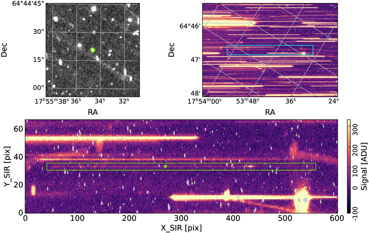
Figure 1: Illustration of the various exposures entering the SIR pipeline for object ID 2684805874647806467, a $z=1.63$ galaxy. Upper left: $50\mathrm{″}$-cutout from the MER $J_{\scriptscriptstyle\rm E}$-band stack, centred on the object (green contour). Upper right: close-up on DET42 of preprocessed background-subtracted RGS000+0 spectroscopic exposure (pointing ID 11953) around the spectrogram of the same object (blue box). Bottom: zoom into the blue box in SIR coordinates; the effective extraction window is indicated as a green box, and the position of the reference wavelength $\lambda_{1}$ is marked with a star, while original pixels flagged as unusable are in grey. We note the bright (saturated) 0th-order spectrogram in the lower right, as well as low-level persistent traces of previously-observed tilted 1st-order and 0th-order spectrograms.

2.3.4 Detector scaling

The purpose of the ‘detector scaling’ is to correct intensity variations within a detector, and across the detectors, due to differences in each pixel’s quantum efficiency (QE). This eliminates not only individual pixel-to-pixel variations on the small scale, but also larger-scale fluctuations in the detector response due to various surface properties, sometimes leading to distinctive ‘islands’ of pixels with lower-than-normal QE (see Euclid Collaboration: Jahnke et al. 2024, Euclid Collaboration: Kubik et al., in prep.). These structures can show spatially abrupt changes in QE, especially at the island boundaries, and need to be corrected to restore spatial continuity at the detector scale (see Fig. 2).

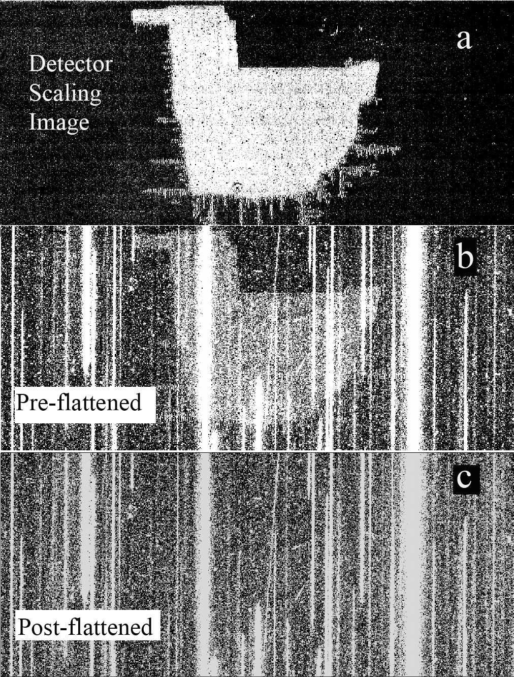
Figure 2: Illustration of the application of the detector scaling product to a small section of the DET11 images: (a) the detector scaling image centred on the ‘duck’ structure (see Sect. 2.4.2); (b) the same section of a dispersed image prior to correction, and (c) after the application of the detector scaling. The ‘duck’ structure has been successfully mitigated.

In order to eliminate intensity variations in the data due to QE variations, the spectroscopic image is divided by a ‘master flat’, one per detector. As explained in Sect. 2.4.2, the master flat is presumed to be achromatic, and computed assuming a uniform illumination scene dominated by the zodiacal background.

We note that, unlike standard photometry (where the mapping between sky and detector positions is bijective), the master flat for dispersed imaging only corrects for detector-scale effects, but cannot account for relative flux calibration at all positions and wavelengths, which are degenerate quantities on the detector; this is therefore specifically adressed by the relative flux scaling (Sect. 2.3.8).

2.3.5 Background subtraction

The ‘background subtraction’ PE is aiming at estimating and subtracting the additional flux component not directly associated with individual spatially-localised sources, e.g., zodiacal diffuse background, scattered, and stray light (diffusion), ghosts (reflections), etc.

By lack of elaborate ghost and stray light models for the spectroscopic channel at time of production, the Q1 version of the pipeline only computes a uniform background value independently for each detector, estimated from the mode of the distribution of the ‘signal-free’ pixels, i.e., not covered by 0th- and 1st-order spectrograms of sources with $J_{\scriptscriptstyle\rm E}\leq 23$, and not masked during preprocessing.

2.3.6 Spectra decontamination

Dispersed imaging – as obtained with Euclid NISP-S – suffers from cross-contamination, i.e., the spectrogram of each source is potentially contaminated by flux from other sources in its vicinity. Although the use of the four different dispersion directions in the observation strategy mitigates the contamination to a certain extent, the sensitivity of Euclid implies there is a large number of potentially-contaminating sources (${10}^{4}{10}^{5}\text{\,}\mathrm{d}\mathrm{e}\mathrm{g}^{-2}$) relative to the number of H$\alpha$ emitters (less than $4000\text{\,}\mathrm{d}\mathrm{e}\mathrm{g}^{-2}$, see Euclid Collaboration: Scaramella et al. 2022; Euclid Collaboration: Gabarra et al. 2023). These H$\alpha$ emitters are used measuring the imprint of the baryon acoustic oscillations on galaxy clustering between $0.9<z<1.8$ to determine the redshift evolution of dark energy, one of the primary science goals of Euclid (Laureijs et al. 2011).

Furthermore, the relatively coarse spatial sampling of NISP ($0.\mathrm{″}3$, Euclid Collaboration: Jahnke et al. 2024) and significant extent of the NISP-S point spread function (PSF, 20% flux outside $0.\mathrm{″}68$) mean that the spatial wings of bright sources can affect many pixels beyond the typical source extraction aperture of five pixels used in the pipeline (see Sect. 2.3.7). As an estimation, there are 10 to 30 sources that overlap the 1st-order spectrogram of each source of interest; this number is even larger in dense regions of sky such as galaxy clusters.

Contamination of the 1st-order spectrogram of a source of interest occurs because the 0th-order and the 1st-order – and possibly other dispersion orders for extremely bright sources – spectrograms of unrelated sources fall on the same region of the detector. In all cases, this will result in an extrinsic dither-dependent flux excess in the extracted spectrum of the target source, degrading both its continuum and its spectral features.

Due to the volume of data being run through the spectroscopic pipeline, there are stringent memory and computing time requirements, which result in limitations on the range of algorithms that can be used for decontaminating the spectra. For the Q1 release, a ‘standard’ decontamination PE was implemented and tested. It identifies all contaminating sources, gathers their positions, brightnesses, and surface brightness profiles from NISP-P imaging data, estimates their (1D) spectrum, builds (2D) pixel-level spectrogram models at their specific locations, and subtracts these models from the spectrogram of each source of interest at each individual roll angle (dither). If the contamination appears too large (above requirements, see below), the contaminated pixels are flagged as unusable, and will not enter the extraction step (see Fig. 5). The procedure is also used to identify and mask out 0th-order spectrograms in the dispersed images.

Contaminant catalogue.

The first step in this process is to compile accurate photometry for all the sources in the field of view. While the NISP-P photometry is accurate for sources fainter than the limit of 16th mag, there is no reliable Euclid measurement for brighter saturated sources (Euclid Collaboration: Jahnke et al. 2024). As mentioned earlier, we address this issue by using the external 2MASS photometry (Skrutskie et al. 2006) to estimate their brightness.

The second step is to use the position, size, and brightness of all the sources in the input source catalogue and corresponding spectra-location table to define the effective area within which the source spectrogram is located. For typical sources, the source size is adopted as the larger of the size in the photometric data and 5 pix; for the brightest sources ($J_{\scriptscriptstyle\rm E}<16$), however, the size of the location table is progressively widened up to 20 pixels (for sources with $J_{\scriptscriptstyle\rm E}<12$) to account for the flux of the wings of the point spread function (PSF), as described earlier. If this were not done, a fraction of sources of interest would still be contaminated by the brightest sources in the field of view.

0th-order masking.

We next use the spectrometric model (Sect. 2.3.3) to mask out the 0th-order spectrograms for all sources. We have estimated that the magnitude threshold at which the 0th-order spectrogram of a source is below the Poisson noise threshold from the background corresponds to $J_{\scriptscriptstyle\rm E}=19.5$. Not only is the 0th-order PSF not as sharp as the 1st-order one, but its extent also depends on its radial position in the FP. Additionally, for bright resolved galaxies, the spatial extent of the source matters as well. For the Q1 release, we have been conservative in the size of the 0th-order masking box by calibrating it on bright stars; however, for bright sources, particularly galaxies detected by 2MASS, the 0th order may still extend beyond the box and be left unmasked, polluting distant spectrograms. An improved modelling and masking of the 0th-order will be included in a subsequent version of the pipeline.

1st-order contaminants.

The location table is used for each source to identify all 1st-order contaminants, i.e., adjacent sources whose 1st-order spectrogram overlap the 1st-order spectrogram of interest. Since the typical spectrogram extent is 531 pixels long and approximately 5 pixels wide, if any of those 2500 pixels include flux from even the wings of an adjacent source, it is classified and listed as a contaminant. In the current pipeline runs, a catalog magnitude cut of $H_{\scriptscriptstyle\rm E}<22.5$ is adopted for identifying the sources and their contaminants. This is partly because of spurious sources being present at fainter magnitudes, likely due to persistence.

Spectral (1D) model of contaminants.

We next estimate the contribution from each identified contaminant to the source of interest. To model the continuum of each contaminant, we adopt two approaches. We first try to model the continuum by fitting a power law to the measured flux densities in the spectrograms over the uncontaminated domains. If a line is strong enough to be seen at $\gg 5\sigma$ in a single spectrogram, it is masked out when deriving the power-law fits to the continuum flux model and then added back in as a Gaussian line to the model. The contaminating source is then defined as ‘bright with detectable continuum’ if the derived continuum is consistent with the $J_{\scriptscriptstyle\rm E}$ and $H_{\scriptscriptstyle\rm E}$ broadband flux densities within 10%; we find that this criterion is matched only for a few percent of sources, mostly because of contamination, and because we have not yet included optimal profile-weighted extraction in the pipeline (see Sect. 2.3.7). For the bright sources fulfilling this consistency criterion, the power-law fit from the spectrogram continuum is used.

For fainter contaminating sources, or sources for which no consistent measurements of the continuum can be obtained from spectrograms, we directly fit a power law to its broadband flux densities. For sources with all $Y_{\scriptscriptstyle\rm E}$, $J_{\scriptscriptstyle\rm E}$, and $H_{\scriptscriptstyle\rm E}$ measurements available from NISP-P, we adopt one power law between $Y_{\scriptscriptstyle\rm E}$ and $J_{\scriptscriptstyle\rm E}$, and another between $J_{\scriptscriptstyle\rm E}$ and $H_{\scriptscriptstyle\rm E}$, with continuity between the two interpolations. For sources missing any NISP-P magnitude, the spectral model falls back to a single power law fit to the 2MASS $J$- and $H$-band flux densities. Various tests have shown that the double power-law results in better residuals than a single power-law.

Spectrogram (2D) model of contaminants.

The next challenge is to spatially distribute the model flux density of the contaminant in the spatial (cross-dispersion) direction to build a contaminating spectrogram. While one would naively adopt the spatial extent of the source in the imaging data, this is inaccurate, since the grism has optical power: the imaging and spectroscopic PSFs are different, with the imaging PSF being narrower. We use an ad hoc wavelength-dependent Gaussian kernel to degrade the source profile derived from the segmented thumbnail extracted from the $J_{\scriptscriptstyle\rm E}$ stack produced by MER (Euclid Collaboration: Romelli et al. 2025). For saturated sources that do not have source profiles measured by MER, we assume that they are point sources; this is obviously inaccurate for bright nearby galaxies and will be revised in the future. Appropriate corrections for the fraction of flux outside the extraction aperture are also applied.

We then take the Gaussian fits to the imaging profiles of the sources and degrade them with the imaging-to-spectroscopic cross-kernel to obtain the estimated wavelength-dependent spatial profile of each source in the spectroscopic data. The model flux densities derived are then distributed chromatically using this spatial profile within its corresponding location table.

Contaminant subtraction.

These modelled spectrograms of all contaminants are finally subtracted pixel-by-pixel from the native spectrogram of the source of interest. This is done for each dither separately on the preprocessed, detector-rescaled, background-subtracted dispersed images. Pixels where the total contaminating flux is larger than 10% that of the source of interest are flagged out for excessive contamination, and do not enter the extraction procedure (Sect. 2.3.7).

The end result from this decontamination process is a decontaminated spectrogram for each source of interest for each dither, along with corresponding bitmask and variance layers (see Fig. 3). The bitmask layers are crucial for identifying which pixels should be ignored either due to the 0th-order contamination or due to excessive contamination from a bright source in the subsequent steps in the pipeline (notably spectrum extraction).

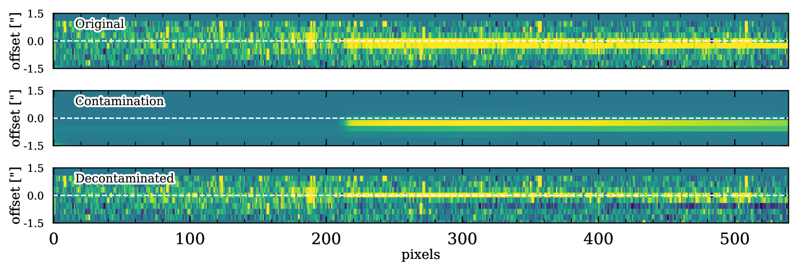
Figure 3: Illustration of the basic decontamination procedure for a line-emitting source. The top panel shows the original RGS000+0 spectrogram of object ID 2709725257636288279 in SIR coordinates, i.e., the $y$-axis being the spatial direction and $x$-axis effectively the dispersion direction. The middle panel shows the model for the bright contaminant, in this case created from broadband photometry, which affects a part of the target spectrogram. The bottom panel shows the decontaminated spectrogram of the source of interest. The flux scaling of all panels is the same.

2.3.7 Spectra extraction

Once the 1st-order spectrogram of a given object has been precisely located within the NISP-S exposure (see Sect. 2.3.3) and properly decontaminated from external sources (see Sect. 2.3.6), one needs to extract and build an estimate of the source spectrum. This includes proper handling of optical distortions and application of the wavelength solution to produce a linear wavelength ramp. This is the objective of the ‘spectra extraction’ PE, which provides both a ‘recti-linear’ 2D spectrogram (not integrated over the cross-dispersion spatial direction) and a 1D spectrum (integrated over the source extent in the cross-dispersion direction).

Spectrogram resampling.

The first step of the extraction is to resample the 2D spectrogram, in order to:

1. align and rectify the spectrogram along the horizontal direction, accounting for mean grism tilt and distortion-induced curvature;

2. include the inverse dispersion solution (IDS) to generate a spectrogram linearly sampled in wavelength in the dispersion direction;

3. move the virtual slit (see below) perpendicular to the dispersion direction to minimise the effective LSF.

The decontaminated spectrogram is resampled a single time using a $4\times 4$ hyperbolic-tangent kernel, with proper handling of masked pixels.

While the wavelength- and distortion-resamplings are classical, the virtual slit deserves more explanation. In order to minimise self-contamination – i.e., the degeneracy between the effective spectral resolution and the spatial extent of the source in the dispersion direction – and therefore improve spectral resolution by minimising the effective LSF, the 2D spectrogram of a resolved source is resampled to align the source maximal elongation in the cross-dispersion direction, the so-called ‘virtual slit’, perpendicular to the dispersion direction (see Fig. 4).

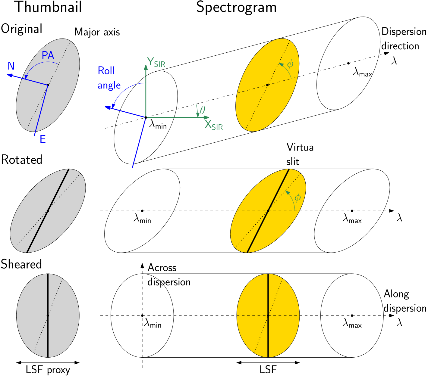
Figure 4: Illustration of the different steps in the extraction of a spectrogram (right) of an extended source, along its photometry thumbnail (left). Top: original orientation in the FP. Middle: rotation to bring the dispersion direction to horizontal. Bottom: shear to bring the virtual slit along the cross-dispersion direction and minimise self-contamination. This illustration is a simplified case with no initial tilt or curvature in the spectral trace; furthermore, in practice, rotation and shear are performed in a single step to minimise correlations between resampled pixels.

In practice, the resampling includes a transformation locally similar to

$$T=\begin{bmatrix}1&m\\ 0&1\\ \end{bmatrix}\begin{bmatrix}\cos\theta&\sin\theta\\ -\sin\theta&\cos\theta\end{bmatrix},\quad\text{with}\quad m=\frac{1-q^{2}}{\tan\phi+q^{2}/\tan\phi},$$ (1)

where $\theta$ is the dispersion direction with respect to horizontal (potentially wavelength-dependent, due to distortions), $\phi$ the source position angle with respect to dispersion direction, and $q$ the flattening of the source (both supposed achromatic). This transformation guarantees that the spectrogram is resampled horizontally, and the virtual slit brought to vertical; as a consequence, the apparent extent of the source along the dispersion direction, which directly sets the effective LSF, is minimised.

For the Q1 release, the actual width of the extraction aperture used by the spectrogram resampling is defined as follows, depending on the nature of the source. For extended objects, the size of the rectified virtual slit is set from the semi-major axis of the source as quoted in the MER catalogue (Euclid Collaboration: Romelli et al. 2025); this size is further limited to five (lower limit) and 31 pixels (upper limit). For point-like objects – defined as objects with a point-like probability $>0.7$ in the MER catalogue or cross-matched in the 2MASS catalogue, the virtual slit is five pixels long.

In addition to the ‘spatial’ components of the resampling (curvature and virtual slit), resulting in a scale of $0.\mathrm{″}3$ $\mathrm{p}\mathrm{i}\mathrm{x}^{-1}$ in the cross-dispersion direction, the resampling transformation also includes the wavelength solution in the spectral direction, so that the resampled spectrogram is linearly sampled along the dispersion direction, from $\lambda_{\min}=$1190.0\text{\,}\mathrm{n}\mathrm{m}$$ to $\lambda_{\max}=$1900.2\text{\,}\mathrm{n}\mathrm{m}$$, with a step of $\delta\lambda=$1.34\text{\,}\mathrm{n}\mathrm{m}$$ for the red grism (531 pixels).

During the resampling process, resampled pixels are a mixture of numerous (up to 16) original pixels, with no longer direct inheritance: all the original quality bits of the input pixels cannot be propagated to the output ones. For this reason, a new bitmask is computed and stored along with the 2D spectrogram (see Table 1). Since the resampling is a weighted average of the pixels within the kernel extent, a final pixel is flagged as:

NOT_USE,

if the numeral fraction of unmasked pixels used during resampling is lower than 25%;

LOW_SNR,

if the same fraction is lower than 50%;

LOW,

if only outer weights of the kernel are used, resulting in a suspicious interpolated value.

Figure 5 shows examples of signal spectrograms after resampling. Following Casertano et al. (2000), the variance layer of the spectrogram is resampled with the same procedure, rather than being propagated.

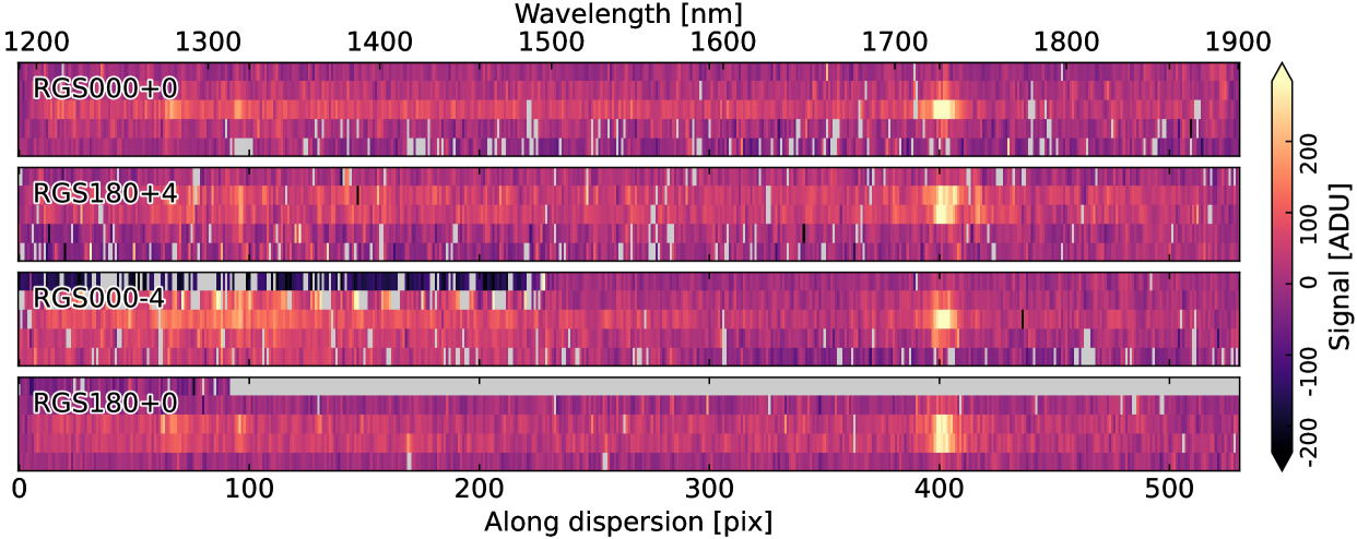
Figure 5: The four $5\times 531$ pixels (corresponding to $$$\times$711.54\text{\,}\mathrm{n}\mathrm{m}$$) resampled spectrograms for object ID 2684805874647806467 (RGS000+0, RGS180+4, RGS000-4 and RGS180+0 from top to bottom) from observation ID 2712. Resampled pixels flagged as unusable (NOT_USE) are in grey.

Averaged summation.

For the Q1 release, the spectral extraction, which generates the 1D spectrum of the source, is performed by averaging unmasked pixels along the cross-dispersion direction, and rescaling by the aperture size, i.e., the width of the 2D spectrogram along the cross-dispersion direction. This ‘averaged summation’ attenuates the impact on flux of masked pixels in the spectrogram.

The 1D bitmask is computed as:

NOT_USE,

if the fraction of unmasked pixels used in the average is lower than 50%;

LOW_SNR,

if the same fraction is lower than 75%.

Figure 6 shows examples of extracted spectra (after relative and absolute flux calibrations).

Line-spread function.

As mentioned earlier, the effective LSF of a slitless spectrum is an intricate mixing of instrumental PSF and intrinsic source extent. While the PSF part can be estimated independently from pure point sources (e.g., stars), the spatial contribution depends on the extended source properties, and presumably varies with wavelength due to colour gradients and distribution differences between stellar and gaseous components.

In practice, the effective extent of the source is estimated from the segmented $0.\mathrm{″}1$ $\mathrm{p}\mathrm{i}\mathrm{x}^{-1}$ thumbnail extracted from the $J_{\scriptscriptstyle\rm E}$ stack produced by MER (Euclid Collaboration: Romelli et al. 2025). The thumbnail at NISP-P resolution ($\sigma\approx$$$) is convolved by a 2D Gaussian to match mean NISP-S PSF ($\sigma\approx$$$), rotated, and sheared according to the spectrogram resampling procedure (see Fig. 4), and finally rebinned by a factor of three to match the NISP spatial scale of $0.\mathrm{″}3$ $\mathrm{p}\mathrm{i}\mathrm{x}^{-1}$. The LSF standard deviation is estimated from a 1D Gaussian fit to the resulting thumbnail marginalised over the cross-dispersion direction.

2.3.8 Relative flux scaling

Large-scale transmission variations in the instrument, arising from a combination of optical and detector effects, must be measured and corrected to ensure consistent flux measurement for sources. To accomplish this, a relative flux scaling solution is derived for each grism/tilt configuration using repeat observations of bright stars in the self-calibration field (see Sect. 2.4.3 for details).

The relative flux scaling is applied to the extracted spectra based on the grism/tilt configuration and the location of the spectrum in the FP. This correction ensures that a consistent instrumental flux (prior to absolute scaling) will be reported for a given source no matter where it lands on the detector/FP, which grism/tilt combination was used, or the epoch of the observation. At present, the relative flux scaling solution appears to be stable with time and hardly chromatic.

2.3.9 Absolute flux scaling

After the relative flux scaling has been applied, each extracted spectrum is divided by a grism- and tilt-specific sensitivity function produced by a dedicated calibration pipeline (Sect. 2.4.4). This converts the instrumental flux units into physical units chosen to be $\mathrm{e}\mathrm{r}\mathrm{g}\,\mathrm{c}\mathrm{m}^{-2}\,\mathrm{s}^{-1}\,\mathrm{\SIUnitSymbolAngstrom}^{-1}$. In this way, each individual spectrum is flux calibrated in an absolute sense, making them intrinsically comparable. The flags associated with the sensitivity product are carried forward in the spectrum bitmask.

2.3.10 Spectra combination

Multiple independent realisations – from different detectors and ROS dithers, potentially from different pointings at their intersections – of the intrinsic spectrum of a given source are combined by the ‘spectra combination’ PE to produce a consolidated – both from a statistic and systematic point of view – estimate of the flux-calibrated source spectrum. This operation is run for every source on a MER tile basis, and combines all spectra for the given source available to date, from pointings covering this tile.

Given the potential issues still affecting individual spectra (e.g., decontamination residuals, unmasked bad pixels, bright 0th-order diffraction spikes, ghosts, etc.), a plain average of the single-dither spectra is not robust enough. On the other hand, given the small number of single-dither spectra to be combined – typically $N\approx 4$ corresponding to the four dithers in an ROS –, a plain median is not statistically efficient.

An outlier-detection scheme, similar to Grubbs’ bilateral test (Grubbs 1969) but using the ‘pull’ in place of the z-score, is therefore run first at the pixel-level among the $N$ flux realisations $f_{i}\pm\sigma_{i}$. For each measurement $i$ of the $N$-sample, its pull $p_{i}$ is defined as

$$p_{i}=\frac{f_{i}-\bar{f}_{i}}{\sqrt{\sigma_{i}^{2}+\bar{\sigma}_{i}^{2}+\sigma_{0}^{2}}}$$ (2)

where $\bar{f}_{i}$ (resp. $\bar{\sigma}_{i}$) is the inverse-variance weighted average (resp. its associated error) of the sample without measurement $i$, and $\sigma_{0}$ is an estimate of the intrinsic (beyond statistical) dispersion among the single-dither spectra (accounting e.g., for flux calibration errors). In practice, outlying flux realisations are defined as $|p_{i}|>p_{\max}=4$. This procedure iteratively identifies and masks out significantly discordant pixels still affected by yet-unflagged bad pixels, decontamination residuals, bright 0th-order diffraction spikes, ghosts, etc.

A standard inverse-variance weighted average is then performed over the $n\leq N$ unclipped values, to compute the combined signal, its associated variance, and set the following bitmask values (see Table 1):

NOT_USE,

if $n<2$ or $n/N<50\%$ (i.e., more than 50% of the flux realisations were clipped out), or if $z>5$, where $z$ is the $z$-score (statistical significance) of the final $\chi^{2}=\sum_{i=1}^{n}p_{i}^{2}$ (i.e., the distribution of selected flux realisations is not compatible with flux errors and intrinsic dispersion);

LOW_SNR,

if $n/N<70\%$ (more than 30% of the flux realisations were clipped out);

EXT_PBR,

if $z>3$ (the distribution of selected flux realisations is barely compatible with flux errors and intrinsic dispersion);

HIGH,

if any $p_{i}>+3$, where $p_{i}$ is the pull of the selected flux realisations.

LOW,

similar to HIGH, but if any $p_{i}<-3$.

Table 1: Description of the bit used in the resampled spectrogram and combined spectrum bitmask. All bits but NOT_USE are warnings of suspicious behaviour.

No	Description
0	NOT_USE	Could not be computed
1	LOW_SNR	Low S/N
2	EXT_PBR	Suspicious spectrum extraction
3	HIGH	Suspected high
4	LOW	Suspected low
5	REL_FLUX	Suspicious relative flux scaling
6	ABS_FLUX	Suspicious absolute flux scaling

Furthermore, the standard deviation of the effective LSF of the combined spectrum is computed as the root mean square (RMS) of the standard deviation of input single-dither LSFs (see Sect. 2.3.7). Figure 6 shows examples of single-dither and combined spectra (after relative and absolute flux calibrations).

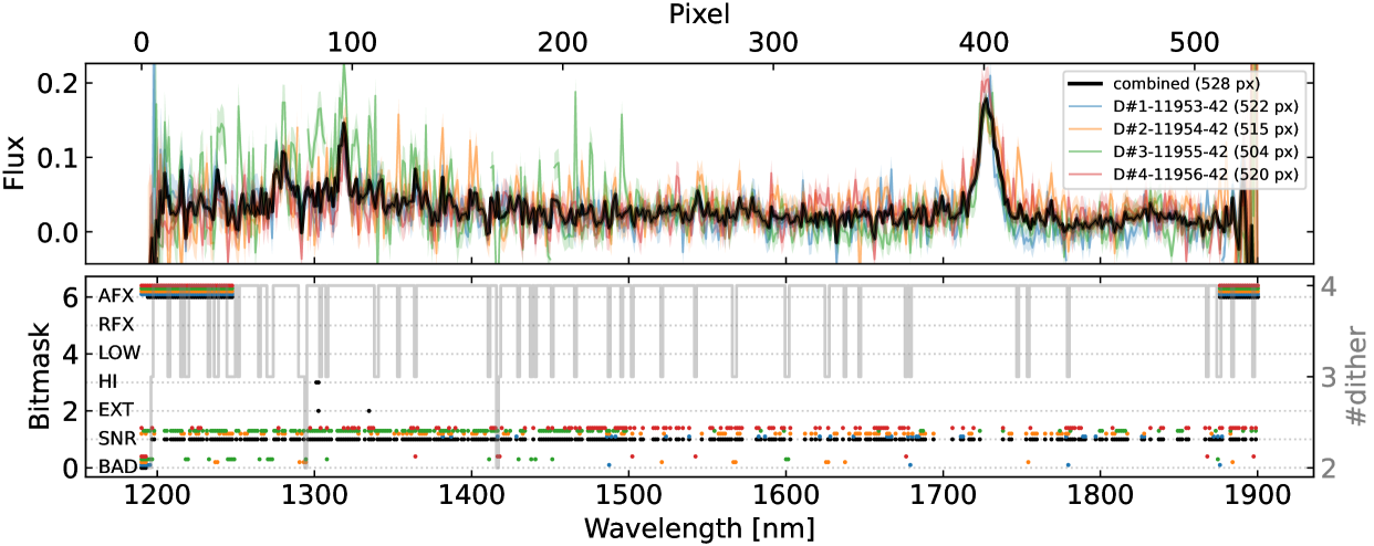
Figure 6: Top: the four single-dither extracted spectra for object ID 2684805874647806467 (coloured), as well as the combined spectrum (black); fluxes are in units of ${10}^{-17}\text{\,}\mathrm{e}\mathrm{r}\mathrm{g}\,\mathrm{c}\mathrm{m}^{-2}\,\mathrm{s}^{-1}\,\AA ^{-1}$. Bottom: individual bit flags (see Table 1) for all the 531 pixels of the single-dither spectra (coloured) and combined spectrum (black), and effective number of pixels that entered the combination (grey).

2.4 Calibration processing elements

The preprocessing calibration PEs are presented in Euclid Collaboration: Polenta et al. (2025), and we describe the relevant information there.

2.4.1 Spectra location calibration

Astrometric modelling (OPT calibration).

This calibration PE aims at deriving an astrometric model, i.e., the mapping between the sky coordinates (RA, Dec) of a source, as identified in the MER catalogue, and the corresponding 1st-order reference position in the FP, first in R-MOSAIC coordinates (in mm, Euclid Collaboration: Jahnke et al. 2024) and ultimately in detector pixel coordinates (through the use of the metrologic layout of the FP): reference positions $(x_{0},y_{0})$ for 0th-order, and $(x_{1},y_{1})$ for the 1st-order, at reference wavelength $\lambda_{1}=$1504\text{\,}\mathrm{n}\mathrm{m}$$ of the stellar spectral Mg I (blended) feature.

This calibration is derived from astrometric calibration pointings, in which numerous bright point sources are observed simultaneously, by mapping sky coordinates to measured 1st-order star absorption positions in the registered exposure. It uses a preliminary mapping specifically derived and validated during the PV phase, as well as the FP metrology to convert FP coordinates (in mm) to detector coordinates (in pixels). We note that the ground-based metrology, derived from measurements at room temperature, was not precise enough; an ad hoc effective metrology was developed – only including translation terms in the Q1 release – to insure spectral continuity between adjacent detectors.

Spectroscopic modelling (CRV and IDS calibrations).

The spectroscopic model (sky position to spectrogram mapping), including spectral distortions and wavelength solution, slightly varies over the FP. The SIR reduction pipeline describes these changes using global spectroscopic models, calibrated using the following two sets of observations.

Curvature model (CRV):

the same astrometric calibration pointings, in which many point (stellar) sources are observed simultaneously, by measuring the cross-dispersion offset of the spectral trace as a function of position along the dispersion axis, to accurately describe the geometrical shape of the spectrogram (spectral distortions).

Wavelength solution (IDS):

dedicated observations during the PV phase of a bright planetary nebula (PN SMC-SMP-20, Euclid Collaboration: Paterson et al. 2023), whereby the planetary nebula (PN) is observed at $16\times 5=80$ different positions in the NISP FP, and the bright emission lines in the PN spectrum are used to derive the mapping $\lambda(D)$ – namely the IDS – between tabulated wavelengths $\lambda$ and measured positions $D$ along the spectral trace. See Figure 15 of Euclid Collaboration: Jahnke et al. (2024) for examples of spectrograms, spectra, and reference wavelengths of PN SMC-SMP-20 used in this procedure.

By constructing the spectroscopic model over the full FP, the calibration procedure allows us to predict for each source, given its coordinates in the sky (but fully independently of its intensity), the geometric and chromatic description of the 0th- and 1st-order spectrograms. As a consequence, SIR PF can handle spectra for any source from the MER catalogue, notwithstanding its magnitude.

2.4.2 Detector scaling calibration

As mentioned in Sect. 2.3.4, the scaling acts as both small- and large-scale flat fields – correcting for detector-related QE fluctuations – but also includes the effective QE conversion factor for each pixel. The pixel-level QE was measured on the ground for all 16 detectors at 40 wavelengths between $600$ and $2550\text{\,}\mathrm{n}\mathrm{m}$, and shows a weak percent-level stochastic dependence on wavelength (Euclid Collaboration: Kubik et al., in prep.). The detector-scaling calibration product (‘master flat’) is a set of $2040\times 2040$ maps (one per detector) representing the effective QE averaged over the ${\rm RG}_{\scriptscriptstyle\rm E}$ passband (see below).

Except for the pixels illuminated by the brightest sources, most of the signal in the pixels in the grism spectroscopic data arises from the zodiacal light, which accounts for about 1000 electrons in a nominal 550 s exposure. The zodiacal light at these wavelengths is assumed to have an intensity power-law spectral density $I_{\nu}\simeq\nu^{-0.8}$ per unit of frequency $\nu$ (Kelsall et al. 1998; Gorjian et al. 2000), which, after conversion to electrons per spectral pixel using the sensitivity curve (Sect. 2.4.4), is used to compute the weighted average of the intrinsic QE values for each pixel. Although uniform weighting by the zodiacal spectrum for all pixels in the field of view is a crude approximation of the complex illumination scene, the QE spatial fluctuations are not significantly chromatic – i.e., $\delta\text{QE}(i,j,\lambda)\approx\delta_{ij}\times\overline{\text{QE}}(\lambda)$ with $\delta_{ij}$ the gray fluctuation of pixel $(i,j)$ – and this approach is therefore well justified. The master flat is the same for all red grism/tilt configurations, but since QE varies with wavelength, it still depends on the grism passband.

Local variations in the QE maps averaged over several hundreds of pixels are typically correcting the input signal at the percent level, whereas the shot-noise in the detectors is typically 3 to 4% in a blank region of the detector for standard exposure times. This means that the application of the flat for a well-behaved part of the image is relatively benign. However, the detector scaling does have a significant net-positive effect, because it also corrects for discontinuities at the boundaries of well identified detector artefacts (e.g., the ‘fish’-shaped region in DET21, or the ‘duck’-shaped structure in DET11, see Figure A.1 of Euclid Collaboration: Jahnke et al. 2024) showing abrupt changes in QE (at the 3 to 5% level). These effects are efficiently handled by the detector scaling product, and lead to a significant flattening of the images after application (see an illustration on the ‘duck’ in Fig. 2).

In the current implementation, the detector scaling calibration does not use the multi-chromatic flat exposures from the internal calibration unit (Euclid Collaboration: Jahnke et al. 2024; Euclid Collaboration: Hormuth et al. 2024), but only relies on ground-based multi-wavelength measurements. It is a foreseen development of SIR PF to estimate and correct for potential time evolution of QE maps from in-flight observations.

2.4.3 Relative flux calibration

The relative flux calibration module computes the relative transmission variations of the instrument as a function of position on the FP, wavelength, time, and the instrumental configuration (grism/tilt) used. These transmission variations are corrected for at the level of a single-dither 1D extracted spectrum in the relative flux scaling PE (Sect. 2.3.8), prior to combination of all the spectra. It is crucial that this module correctly estimates the transmission variations in order to ensure consistent flux measurements for the mission.

The spectral flux measured for the same source observed at different locations on the FP will vary due to transmission (spatial) fluctuations of the instrument, arising from a combination of optical and detector effects. For example, vignetting on the order of 10% at one edge of the focal plane is expected for acquisitions at the $\pm$$$ tilted-grism positions (Euclid Collaboration: Mellier et al. 2024). Moreover, the large-scale flat pattern may be chromatic, differing at the blue and red end of the grism spectra.

To measure and correct for this effect, we use repeat observations of bright ($16<H_{\scriptscriptstyle\rm E}<18$) stars at random positions in the self-calibration field (Euclid Collaboration: Aussel et al. 2025). Such a large-scale retrospective relative spectrophotometric self-calibration procedure has been described and tested in Markovič et al. (2017), and a working version of it has also been implemented for NISP-P (Euclid Collaboration: Polenta et al. 2025). The dithering pattern of the Euclid self-calibration observations ensures that sources will illuminate different parts of the same detector, different detectors in the focal plane, at different epochs, and with different grism/tilt configurations, thus providing the necessary constraints to map variations in the large-scale response of the instrument. The extracted spectra used for calibration have low levels of contamination (or have undergone successful decontamination). By sampling the same sources at different positions on the focal plane, we build up statistical constraints on the large-scale flat pattern that needs to be corrected to ensure consistent flux measurements regardless of source position.

In practice for the Q1 release, the large-scale response is found to be nearly achromatic, and therefore, to maximise the S/N of the solution, an achromatic solution is derived for all wavelengths that depends only on the position of the observation on the focal plane (see Fig. 7). This solution shows similarities to the NISP-P large-scale flat (Euclid Collaboration: Polenta et al. 2025) and displays the vignetting pattern in the tilted grism configurations expected based on optical simulations of the instrument. It is also shown to correct repeated spectra of bright sources such that they are in agreement. At present, the solution appears to be stable with time, and will be monitored for evolution as the mission progresses.

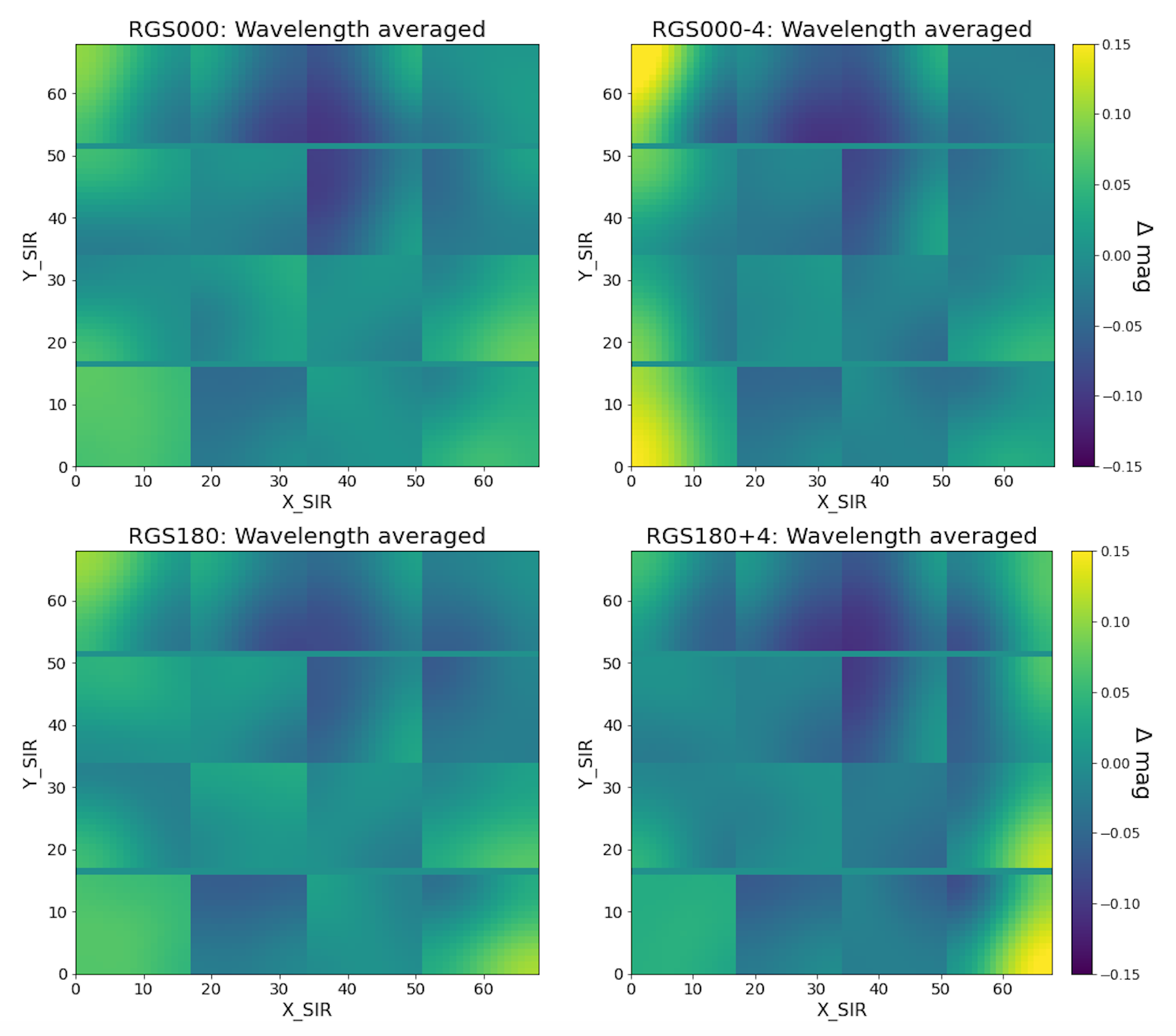
Figure 7: Relative flux solution in SIR coordinates derived for the four grism/tilt configurations by the relative flux calibration. The value $\Delta$mag indicates the correction in magnitude that should be applied to the portion of a spectrum landing at the given focal plane position. The vignetting at the focal plane sides in tilted configurations RGS000-4 (top right) and RGS180+4 (bottom right) is apparent, as are large-scale features in common with the imaging flux solution (so-called ‘flat field’, Euclid Collaboration: Polenta et al. 2025). This solution is found to be mostly achromatic, and is therefore averaged over wavelength.

2.4.4 Absolute flux calibration

The absolute flux calibration pipeline is designed to create a sensitivity function that is used to convert instrumental signal units (electrons per sampling element) into astrophysical flux units ($\mathrm{e}\mathrm{r}\mathrm{g}\,\mathrm{s}^{-1}\,\mathrm{c}\mathrm{m}^{-2}\,\AA ^{-1}$, see Sect. 2.3.9). The sensitivity function was created by first averaging repeat observations of the flux calibration star GRW+70 5824, a DA2.4 white dwarf (Gianninas et al. 2011) acquired during the PV phase in a pattern of five points on each detector (Euclid Collaboration: Jahnke et al. 2024), independently for each of the four red grism/tilt combinations (RGS000+0/-4, RGS180+0/+4). For the Q1 release, a separate sensitivity function is created for each grism/tilt combination from the pull-clipped average of $16\times 5=80$ single-dither spectra (after relative flux scaling) of the standard star.

After the single-dither spectra of the reference star have been suitably extracted and averaged, we convert the instrumental flux units into units of $\mathrm{e}\,\mathrm{s}^{-1}\,\AA ^{-1}$, and then divide by a suitably-matched reference spectrum. The reference spectrum used was a model spectrum from CALSPEC (Bohlin et al. 2020), resampled to $0.1\text{\,}\mathrm{n}\mathrm{m}$, convolved to an effective spectral resolution of $3.3\text{\,}\mathrm{n}\mathrm{m}$ (close to the spectral resolution of the red grism for a point source), and resampled onto the SIR wavelengths. The Q1 sensitivity curves for the four grism/tilt configurations are shown in Fig. 8.

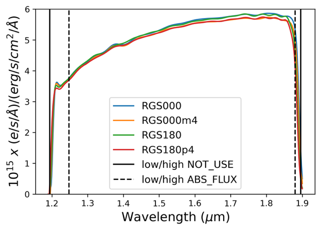
Figure 8: Sensitivity functions for the four red grisms (RGS000+0/-4, RGS180+0/+4), derived from PV observations of the white dwarf GRW+70. The vertical black solid and dashed lines represent the boundaries of the NOT_USE and ABS_FLUX (suspicious) flags. In this figure, we show the limits for RGS180+0, but each grism/tilt configuration has slightly different limits.

The bitmask layer is used to flag the sensitivity function, wavelength by wavelength: for the Q1 release, the NOT_USE flag is set on domains where the sensitivity function deviates by more than 5% from pre-launch expectations; and the ABS_FLUX (suspicious) flag is intended to emphasise spectral domains where the throughput is less than 80% of the maximum throughput at the band edges. We note that, during the Q1 production, a software error led to some excess flagging of ABS_FLUX pixels on the blue-side of the spectral domain (see Figs. 6 and 8); this problem has been resolved for future releases.

2.5 Q1 validation and data quality control

2.5.1 Validation pipeline

The current validation process for the SIR PF encompasses more than 20 test cases, designed to ascertain the conformity of the pipeline and its data products with the established requirements. The principal objective of the validation tests is to evaluate in detail the performance of each PE of the scientific pipeline, from the spectra location to combination (see Sect. 2.3). The quality of the data is instead assessed on a statistical basis through the Data Quality Control procedure (see Sect. 2.5.2). Validation tests are typically conducted on designated reference fields to assess the impact of modifications and improvements introduced in each pipeline release.

To validate the SIR pipeline used for the Q1 release, we selected four dithered pointings in an ROS over the COSMOS field (Scoville et al. 2007), one of the Euclid ancillary fields including a multitude of additional data and redshifts employed for validation purposes. We present here the results of two of the most significant validation tests, namely those that evaluate the accuracy of wavelength and flux calibration, respectively. These can provide an overall assessment of the performance of the entire pipeline.

Figure 9 illustrates the outcome of the test on the accuracy of the wavelength solution. The histogram shows the difference along the dispersion axis between the nominal position of the blended Mg I absorption line $\lambda$1504\text{\,}\mathrm{n}\mathrm{m}$$ and the position measured on the spectra in a single pointing for bright stars pre-selected in the 2MASS catalogue ($12\leq J_{{\scriptscriptstyle\rm 2MASS}}\leq 16$). The distribution has a normally-scaled median absolute deviation (sMAD) of approximately 0.5 pixel, marginally higher than the requisite 0.4 pixel ($0.54\text{\,}\mathrm{n}\mathrm{m}$). It appeared a posteriori that this slight non-conformity in the Q1 production was mostly due to errors in automatic identification and measurement of the Mg I stellar feature; the procedure has been improved for future releases.

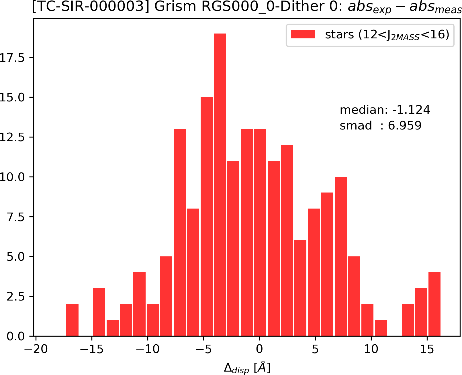
Figure 9: Distribution of the differences along the dispersion axis (in Å) between expected and measured positions of the Mg I absorption feature used as reference in the 1D extracted spectra for a sample of bright stars. Results are presented for grism RGS000+0 in a single pointing.

The accuracy of the flux calibration is shown in Fig. 10. This plot displays the difference between the $J_{{\scriptscriptstyle\rm 2MASS}}$ magnitudes and the magnitudes measured on the 1D spectra in a $50\text{\,}\mathrm{n}\mathrm{m}$ domain around the $J_{{\scriptscriptstyle\rm 2MASS}}$ effective wavelength ($1235\text{\,}\mathrm{n}\mathrm{m}$) in a single-dither pointing, for bright stars ($12\leq J_{{\scriptscriptstyle\rm 2MASS}}\leq 17$). The distribution is centred around a median offset of $-0.01$, with an sMAD of $0.04$ consistent with flux calibration objectives.

Figure 10: Comparison between the $J_{{\scriptscriptstyle\rm 2MASS}}$ magnitudes and magnitudes estimated from single-dither spectra in a $50\text{\,}\mathrm{n}\mathrm{m}$-wide region around $J_{{\scriptscriptstyle\rm 2MASS}}$ effective wavelength ($1235\text{\,}\mathrm{n}\mathrm{m}$) for bright stars in an RGS000-4 pointing. The black solid and dashed lines represent the 40-point running median and sMAD, respectively.

2.5.2 Data quality control

The SIR PF includes the calculation of a number of data quality control (DQC) parameters at each data-processing step. These parameters are critical in assessing the quality of incoming data and identifying potential calibration or reduction problems. The DQC parameters are statistical quantities, calculated on each archived data product using pre-selected sources (e.g., bright stars) or regions of the sky (e.g., excluding bad or contaminated pixels). They are computed on the fly within each PE, in both the calibration and scientific pipelines, and then stored in the Euclid archive system in the XML metadata associated with each data product (e.g., DpdSirScienceFrame, DpdSirCombinedSpectraCollection, etc.). By collecting all DQCs on hundreds of observations, we can get an overview of the general trend of each parameter and thus the average quality of the data. It is beyond the scope of this paper to provide an exhaustive and complete description of all SIR PF DQC parameters. Instead, the following discussion will focus on some of the key parameters derived from the scientific pipeline for the Q1 data processing. This will illustrate the method used for data validation and the quality of the Q1 release.

2.5.3 Quality control for Q1 data set

The SIR data released in Q1 include 117 observations with red grisms, each ROS consisting of four dithers obtained with the different grism/tilt configurations (RGS000+0/-4, RGS180+0/+4). In this section, we present the results for the Q1 release in relation to the following quantities, derived at each run of the SIR scientific pipeline for each detector on sub-samples of point sources (typically 10 to 30 per detector).

DQC.1:

difference (in pixels) between the measured and expected position of the 1504-nm absorption feature on the 1st-order spectrograms along the dispersion axis for bright point sources ($12<J_{{\scriptscriptstyle\rm 2MASS}}<16$). This is related to the accuracy of the spectra location (Sect. 2.3.3), and in particular to the optical model and zero-point of the wavelength solution (Sect. 2.4.1);

DQC.2:

difference (in pixels) between the measured and predicted peak position (of the cross-dispersion profile) along the spectrograms at seven different wavelengths for bright point sources ($12\leq J_{{\scriptscriptstyle\rm 2MASS}}\leq 16$). This is also probing the validity of the spectra location, in relation to the curvature model (Sect. 2.4.1).

DQC.3:

difference between $J$-band magnitudes measured on the spectra and those from the 2MASS catalogue for point sources with $16\leq J_{{\scriptscriptstyle\rm 2MASS}}\leq 18$, probing the reliability of the overall flux calibration (Sects. 2.3.9 and 2.4.4).

The median and sMAD per detector of each DQC parameter are stored in the metadata of the SIR products. Given their derivation from the difference between a predicted and a measured quantity, a positive outcome of the DQC parameters is associated with a median value close to zero and an sMAD within a specified threshold. In order to evaluate a single DQC criterion for each quantity, extending Knig–Huygens formula, the sum in quadrature of the median and sMAD is used as a robust estimate of the RMS:

$$\rm rRMS=\sqrt{\rm median^{2}+sMAD^{2}}.$$ (3)

This is illustrated in Fig. 11, showing the distribution of the robust RMS obtained for the Q1 release for all three DQC parameters; in each case, the distribution is reasonably well represented by a log-normal PDF. A specific pointing may exhibit anomalies if any DQC parameter yields outliers for more than three detectors in these distributions. Similarly, a standard ROS observation may be problematic if more than two grisms fail the DQC threshold. Some outlying detectors were identified in Fig. 11 (i.e., $\gtrsim 5\sigma$ away from the median RMS value), but in most cases, these are from different pointings. In cases where more than three detectors per pointing exhibited outliers, an investigation was carried out.

Figure 11: Top: distribution of the robust RMS of the spectrogram reference position offsets (DQC.1) for the Q1 release. The vertical solid line is the median of the distribution and the solid curve is the log-normal PDF. Middle: same as above but for the cross-dispersion peak-position offsets (DQC.2); since the results are not significantly chromatic, we show the robust RMS averaged over the seven wavelengths. Bottom: same as above but for $J$-band magnitude offsets (DQC.3).

While not all the Q1 spectroscopic data release is strictly within the specified requirements, no invalidating systematic errors were identified. In conclusion, this first Q1 release is considered to be of reasonable accuracy level, in line with the initial performance of the SIR pipeline, and there are reasons to be confident that it will further improve in future releases.

3 Validation of spectroscopic requirements

In this section, we briefly assess the spectroscopic performance of the NISP instrument and SIR pipeline from on-orbit observations, in regard to Euclid’s top-level mission requirements (Euclid Collaboration: Mellier et al. 2024). Since the Q1 release only covers red-grism observations from the EWS, we do not address here the specificities of the blue grism and the deep survey.

We note that flux requirements have not been evaluated at the Q1 stage, and are therefore not addressed here. Preliminary analyses show that flux performance (relative flux accuracy and flux limits) are globally on par with requirements, but we postpone in-depth (red/blue, wide/deep) analyses and validations to later SIR PF publications.

3.1 Spectral resolution

Euclid’s top-level requirement on spectral resolution (actually resolving power) of red-grism observations states:

“The NISP spectrometric channel spectral resolution considering a reference $0.\mathrm{″}5$-diameter source shall be $\mathcal{R}=\lambda/\Delta\lambda>380$ over the $12501850\text{\,}\mathrm{n}\mathrm{m}$ spectral range.

Note: resolution element ($\Delta\lambda$) is defined as the minimum wavelength separation at which two spectral lines produced by a $0.\mathrm{″}5$ object and with the same equivalent width can still be separated.”

This requirement specifically refers to the Sparrow criterion (Sparrow 1916; Jones et al. 1995), for which the physical resolution element (in pixels) is $r(\lambda)=2\sigma(\lambda)$ in the Gaussian approximation. Given the native spectral sampling $s(\lambda)\triangleq\mathrm{d}\lambda/\mathrm{d}D$ (in $\mathrm{n}\mathrm{m}\,\mathrm{p}\mathrm{i}\mathrm{x}^{-1}$, before any spectral resampling), one defines the resolving power as

$$\mathcal{R}\triangleq\frac{\lambda}{\Delta\lambda}=\frac{\lambda}{2\sigma(\lambda)\,s(\lambda)}.$$ (4)

The native spectral sampling $s(\lambda)$ is estimated from measured positions, directly in R-MOSAIC coordinates, of significant emission lines in the PN SMC-SMP-20 spectrograms acquired all over the FP during the PV phase (see Figure 15 of Euclid Collaboration: Jahnke et al. 2024, for an illustration). Overall, the sampling is not found to be significantly dependent on positions in the FP, on wavelength, or on red grism/tilt combination, and hence we adopt the following constant value:

$$s=$1.368\pm 0.025\text{\,}\mathrm{n}\mathrm{m}\,\mathrm{p}\mathrm{i}\mathrm{x}^{-1}$\quad(\text{median}\pm\text{sMAD}).$$ (5)

This value is, as it should be, slightly larger than the adopted spectral bin after wavelength resampling ($\delta\lambda=$1.34\text{\,}\mathrm{n}\mathrm{m}$$, see Sect. 2.3.7).

Under the assumption of an axisymmetric PSF, the intrinsic resolution $\sigma$ of NISP-S is evaluated during the CRV calibration (Sect. 2.4.1) from Gaussian error-function fits to the cross-dispersion profiles of 1st-order spectrograms of bright-yet-unsaturated point sources (approximately 20 per detector). The collection of measurements – for all stars and wavelengths – is then robustly combined into five spectral bins over the spectral extent (see Fig. 12), without noticeable variations over the FP. As expected from instrumental design, the spectral resolution does not show any significant differences between grism/tilt configurations.

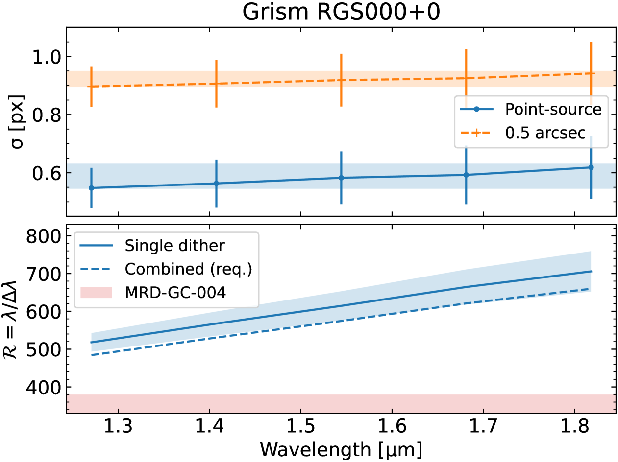
Figure 12: Top: distribution (median $\pm$ sMAD) of intrinsic spectral resolution $\sigma$ (in blue) and effective $0.\mathrm{″}5$-source $\sigma_{e}$ (in orange) for RGS000+0 (pointing ID 266626). Bottom: corresponding resolving power $\mathcal{R}$, for a single-dither spectrum (continuous line) and a 4-dither combined spectrum (dashed line), assuming an as-required wavelength accuracy (38% of a resolution element, see text); the red zone corresponds to the requirement from top-level mission document.

In dispersed imaging, the resolution element is directly degraded by the source extent projected onto the dispersion direction (see Sect. 2.3.7). The requirement refers to a fiducial $0.\mathrm{″}5$ source, understood as the full width at half maximum of an axi-symmetric Gaussian source. With a nominal NISP pixel scale of $0.\mathrm{″}3$ $\mathrm{p}\mathrm{i}\mathrm{x}\mathrm{e}\mathrm{l}^{-1}$, this corresponds to a self-contamination contribution to the resolution of $\sigma_{\text{c}}=$0.710\text{\,}\mathrm{p}\mathrm{i}\mathrm{x}\mathrm{e}\mathrm{l}$$, to be added in quadrature to intrinsic resolution $\sigma$ estimated from point sources (see Fig. 12). We note that, while the cross-dispersion profile is significantly under-sampled for point sources ($\sigma\approx$0.6\text{\,}\mathrm{p}\mathrm{i}\mathrm{x}\mathrm{e}\mathrm{l}$$), it becomes reasonably sampled for $0.\mathrm{″}5$ distant galaxies, Euclid’s primary targets.

Ultimately, the resulting resolving power $\mathcal{R}$ is computed from the effective resolution $\sqrt{\sigma^{2}+\sigma_{\text{c}}^{2}}$, and shown in Fig. 12, along with Euclid’s top-level requirement.

The spectral resolution can be computed either from individual ‘single-dither’ spectra or on ‘combined’ (multi-dither) spectra. The later estimate should therefore include a contribution from the residual wavelength solution errors, since the wavelengths may not be exactly aligned and a spectral feature is artificially broadened by the IDS inaccuracies. If, in the worst-yet-acceptable-case scenario, the wavelength accuracy only marginally meets requirement (38% of a resolution element, see below), its effective contribution to the resolution element is a net increase by approximately $\sqrt{1+0.38^{2}}-1=7\%$ (see Fig. 12).

In conclusion, the resolving power for a reference $0.\mathrm{″}5$-diameter source is compatible with $\mathcal{R}\approx\text{$500700$}$, well above Euclid’s top-level requirement, $\mathcal{R}>380$ for the red grisms. It does not show significant dependence on FP position and grism/tilt configuration. This seemingly high resolving power is a direct indication of the superb quality of the NISP-S optics; we note, however, that it is also dependent on the specific adopted definition of the resolution element.

3.2 Wavelength accuracy

Regarding wavelength accuracy, Euclid’s top-level requirement reads:

“After calibration, the maximum error in the measured position of a spectral feature in the NISP red spectrometric channel ($12501850\text{\,}\mathrm{n}\mathrm{m}$) shall be $<38\%$ of one resolution element.”

An analysis of the wavelength accuracy is performed for grism RGS000+0 from intermediate quantities obtained during the IDS calibration (Sect. 2.4.1) applied to spectrograms of PN SMC-SMP-20. The wavelength accuracy is estimated from the robust RMS error of the expected (calibrated) wavelength position compared to the observed one (the emission line position). The resolution element, presented in Sect. 3.1 for a point source, has been converted to account for the $\sigma_{\text{PN}}=$0.37\text{\,}\mathrm{p}\mathrm{i}\mathrm{x}\mathrm{e}\mathrm{l}$$ extent of PN SMC-SMP-20 (80%-energy radius $r_{80\%}=$$$, Euclid Collaboration: Paterson et al. 2023).

Finally, the wavelength accuracy, i.e., the wavelength RMS error in units of resolution element, is computed per detector and reference line. Its distribution does not show strong chromatic or spatial variations (as a function of wavelength and detector in the FP), and the marginalised distribution is shown in Fig. 13, along with Euclid’s top-level requirement.

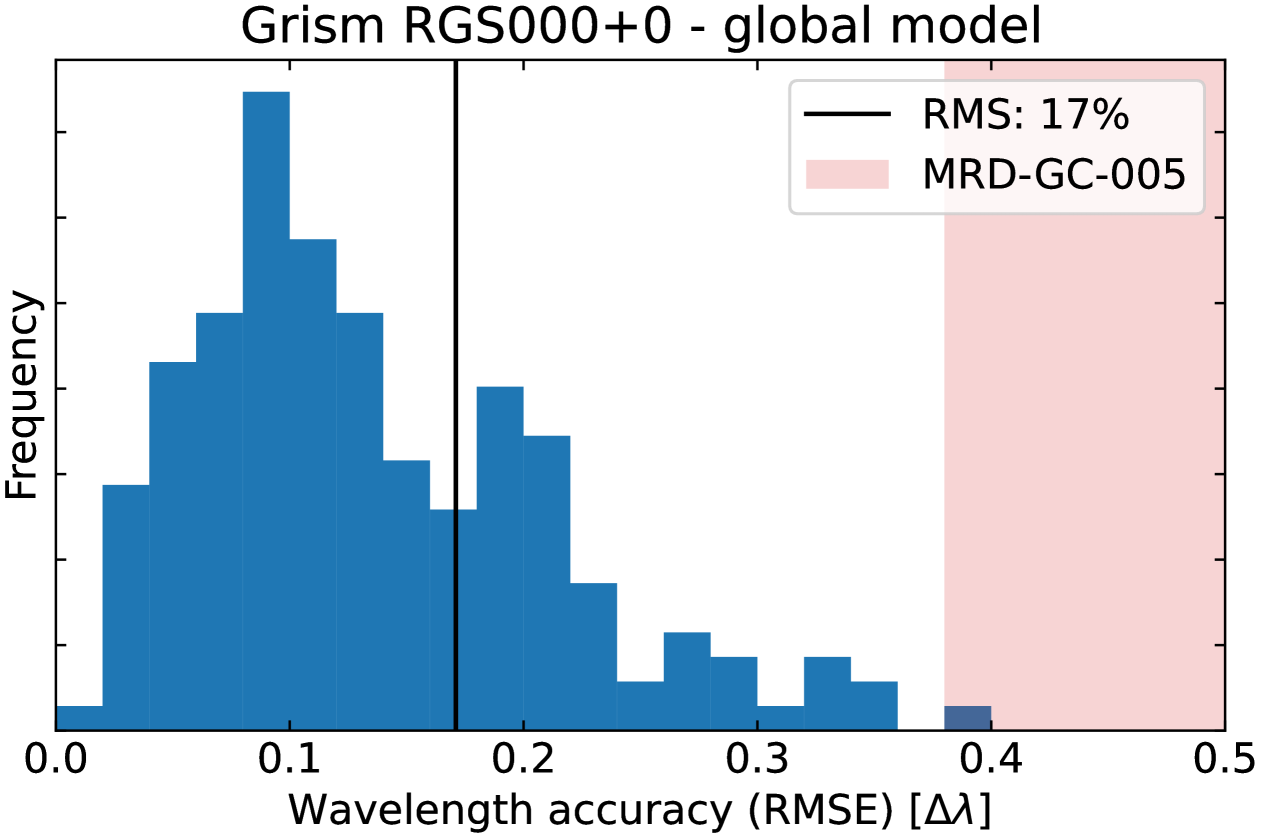
Figure 13: Overall wavelength accuracy distribution for the RGS000+0 IDS (RMS error in units of resolution element $\Delta\lambda$, marginalized over all wavelengths and detectors). The red zone corresponds to the maximum error as stipulated in top-level mission requirements document.

Overall, the IDS delivers an estimated mean wavelength accuracy of $0.23\text{\,}\mathrm{p}\mathrm{i}\mathrm{x}$, corresponding to only 17% of the effective resolution element for SMC-SMP-20 (averaged over wavelengths and detectors in the FP), well below the requirement of 38%. Even though a similar analysis has not been performed on other grism/tilt configurations (namely RGS180+4, RGS000-4, and RGS180+0) at the time of the Q1 release, it is expected that a similar wavelength accuracy would be obtained with these analogous optical configurations.

We note, however, that this analysis is a lower limit, since the wavelength accuracy has been evaluated on wavelength reference PN SMC-SMP-20 itself, a bright ($J\simeq 15.9$) and compact ($r_{80\%}=$$$) source not exactly representative of the $0.\mathrm{″}5$ galaxies that will constitute the core of the Euclid sample. Yet, the overall wavelength accuracy is confirmed by more general pipeline validation analyses (see Sect. 2.5.1), even though it is limited to bright stars and the reference spectral feature Mg I wavelength ($1504\text{\,}\mathrm{n}\mathrm{m}$). It has been repeatedly found that the robust RMS of the wavelength scatter is around $0.7\text{\,}\mathrm{n}\mathrm{m}$ (see Fig. 9), which corresponds to an error of less than 30% of the effective resolution element for a $0.\mathrm{″}5$ source (see Fig. 12). Ultimately, a consolidated assessment of the wavelength accuracy will come from redshift measurements of reference galaxies performed by SPE PF (Euclid Collaboration: Le Brun et al. 2025).

4 Conclusions and planned future work

In this paper, we have detailed the status of the SIR slitless spectroscopy science, calibration, and validation pipelines, as well as its interfaces and principal data products, at the time of the Q1 release (Euclid Quick Release Q1 2025). The SIR PF, with a codebase exceeding $150\,000$ lines – primarily written in Python and C++ – is designed to address the complexities of slitless spectroscopy data from the NISP instrument on board Euclid.

The final Q1 spectroscopic sample includes 4.314 million entries out of the 5.134 million sources with $H_{\scriptscriptstyle\rm E}\leq 22.5$ catalogued by the MER PF over an area of $63.2\text{\,}\mathrm{d}\mathrm{e}\mathrm{g}^{2}$ (Euclid Collaboration: Aussel et al. 2025). Considering only combined spectra originating from at least two dithers (to make the outlier clipping meaningful during combination), 3.778 million spectra have at least one ‘valid’ pixel (Fig. 14), defined as pixels not flagged as NOT_USE or ABS_FLUX (see Fig. 8), and 2.343 million with 300 valid pixels or more (up to 468 pixels). As expected from the ROS, a vast majority (92%) of the spectra results of the combination of three or four dithers, but a substantial number of spectra are computed from eight dithers or more (17733 with at least 400 valid pixels).

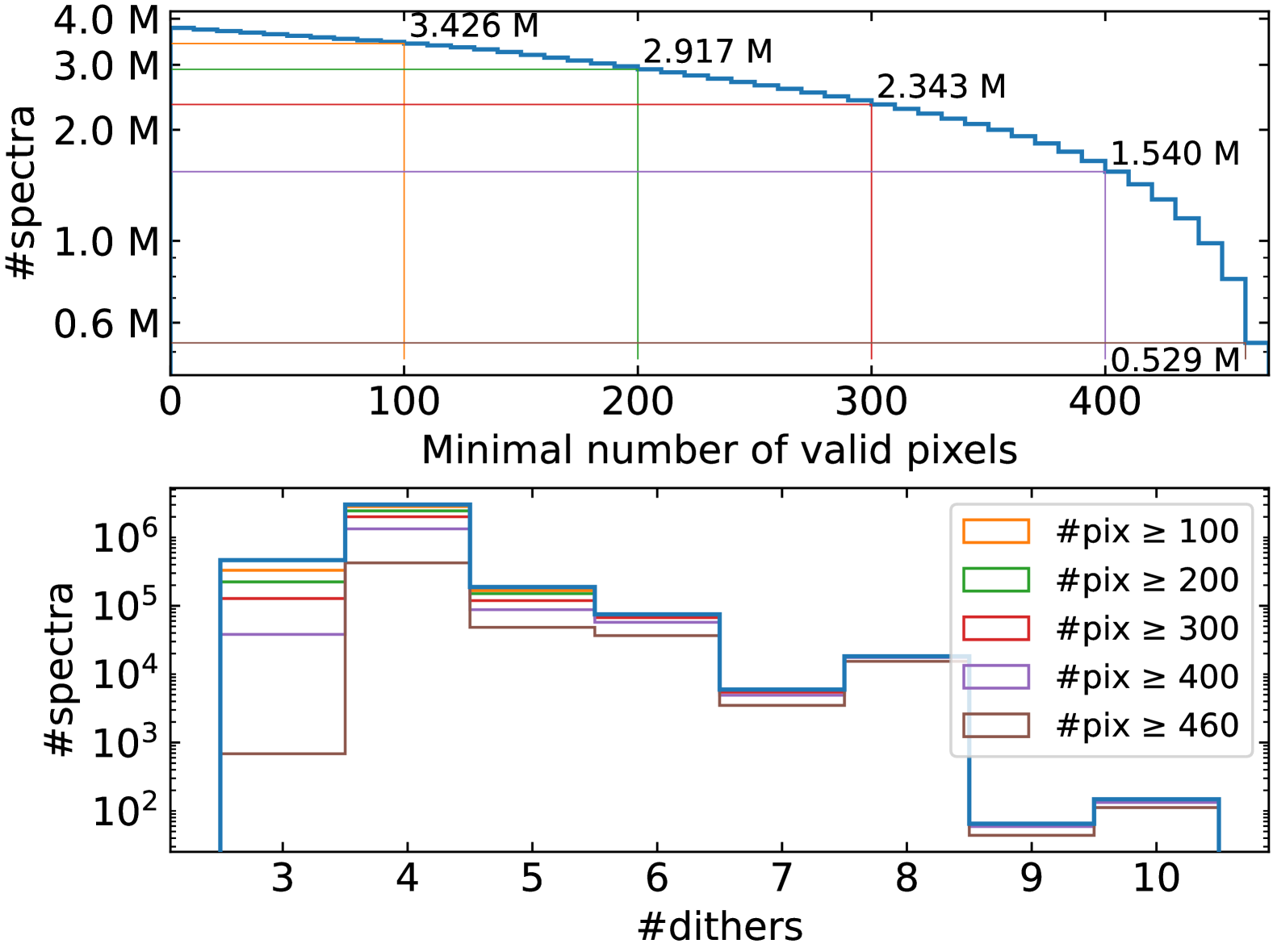
Figure 14: Top: distribution, in the Q1 release, of the number (in millions) of combined spectra originating from at least two dithers with a minimal number of ‘valid’ pixels (see text). Bottom: distribution of the number of dithers included in the spectra combination, as a function of the minimal number of valid pixels.

We also reported spectroscopic performance in favorable agreement with top-level mission requirements, in particular regarding the resolving power $\mathcal{R}\approx\text{$500700$}$, thanks to the exquisite optical quality of the instrument.

We are fully aware of the current limitations and shortcomings of the pipeline, and we urge end-users of SIR spectra to validate them thoroughly before drawing any scientific conclusion (see Euclid Collaboration: Le Brun et al. 2025). However, the modular and flexible structure of the SIR pipelines ensures that it can continuously evolve, with ongoing improvements and refinements at each step of the data calibration and reduction process. The ability to integrate new methodologies, enhance existing algorithms, and incorporate feedback from the scientific community will guarantee that the pipeline remains robust and adaptable to future requirements.

For the forthcoming first data release (DR1, in prep.), several major improvements are being implemented, notably:

• improved FP metrology, accounting for translation and rotation of the detectors in the FP;

• updated Gaussian error-function-based curvature and NISP-S chromatic PSF models;

• incorporation of an optimal extraction (Robertson 1986; Horne 1986) based on cross-dispersion profiles derived from NISP-S PSF-matched MER thumbnails;

• integration with the spectroscopic survey visibility mask estimation process, interfacing with both the SIM and LE3 PFs, respectively in charge of Euclid data simulations and cosmology analyses.

Looking beyond DR1, the pipeline will continue to evolve, with several promising improvements addressing further technical issues: persistence correction on spectroscopic exposures (Kubik et al. 2024); masking and/or subtraction of ghosts and stray light (building on Euclid Collaboration: Paterson et al., in prep.); improved background subtraction methods (e.g., Akhlaghi & Ichikawa 2015); the introduction of a dedicated model for 0th-order masking/subtraction, accounting for its complex shape and position-dependent variations across the FP. The pipeline shall also address the challenges posed by dispersion direction jitter (due to $\lesssim$$$-RMS fluctuations in the GWA position), and extend its decontamination capabilities to spectrograms from $-1$ and $+2$ dispersion orders. To ensure large-scale flux accuracy requirements, it should also implement an bercal flux-calibration scheme (Padmanabhan et al. 2008; Markovič et al. 2017).

Ultimately, the SIR PF could move to more advanced dispersed imaging methods, like advanced decontamination strategies (e.g., Bella et al. 2022), and other forward-modelling techniques (Ryan et al. 2018; Rubin et al. 2021; Neveu et al. 2024) to further enhance the reliability and precision of the extracted spectra. However, one has to keep in mind that these improved algorithms have to match the constraints on memory and computing time from the SGS; it is therefore foreseen that these developments would need to be restricted to a fraction of selected targets of interest among the approximately $50\,000$ sources of a typical NISP-S exposure.

In conclusion, the SIR processing function represents a significant achievement in the reduction of slitless spectroscopic data for the Euclid mission. As the survey progresses, along with our knowledge of the NISP-S instrument, the SIR PF ongoing development, coupled with its modular design, ensures that it will remain a key tool for advancing cosmological and astrophysical research.