Euclid Quick Data Release (Q1)

This paper describes the near-infrared processing function (NIR PF) that processes near-infrared images from the Near-Infrared Spectrometer and Photometer (NISP) instrument onboard the Euclid satellite. NIR PF consists of three main components: (i) a common pre-processing stage for both photometric (NIR) and spectroscopic (SIR) data to remove instrumental effects; (ii) astrometric and photometric calibration of NIR data, along with catalogue extraction; and (iii) resampling and stacking. The necessary calibration products are generated using dedicated pipelines that process observations from both the early performance verification (PV) phase in 2023 and the nominal survey operations. After outlining the pipelines structure and algorithms, we demonstrate its application to Euclid Q1 images. For Q1, we achieve an astrometric accuracy of 9–15 mas, a relative photometric accuracy of 5 mmag, and an absolute flux calibration limited by the 1% uncertainty of the Hubble Space Telescope (HST) CALSPEC database. We characterise the point-spread function (PSF) that we find very stable across the focal plane, and we discuss current limitations of NIR PF that will be improved upon for future data releases.

1 Introduction

Euclid was designed to study the dark Universe through a photometric and spectroscopic survey of the extragalactic sky in the visible and near-infrared bands. An overview of this European Space Agency (ESA) mission, the survey, the data products, and its science programme is presented in Euclid Collaboration: Mellier et al. (2024). The Euclid Wide Survey (EWS, Euclid Collaboration: Scaramella et al. 2022) will cover about $14\,000\,\rm{deg}^{2}$, providing tens of thousands of images to extract positions, shapes, and photometric redshifts for 1.5 billion galaxies, as well as 35 million spectroscopic redshifts. To manage and process these data in a largely automated manner, the Euclid Consortium has built a number of software pipelines and tools constituting the Science Ground Segment (SGS), which has been designed, developed, and validated through a series of data challenges and simulations (Euclid Collaboration: Castander et al. 2024) during the last 10 years, in parallel with the development of the instruments.

In this paper, we describe the NIR PF, which produces calibrated near-infrared images for the Euclid Quick Release Q1 (2025), starting from raw photometric exposures acquired by NISP (see Sect. 2 and Euclid Collaboration: Jahnke et al. 2024). This is achieved through three main steps (Sect. 3): (i) pre-processing to account for instrumental and detector effects that are common to both photometric and spectroscopic exposures (Euclid Collaboration: Copin et al. 2025); (ii) image astrometric and photometric calibration, and catalogue extraction; and (iii) resampling and stacking. The latter step will be described for a future data release, since NIR stacks and associated source catalogues are not part of the Q1 release. The relevant calibration products have been generated through dedicated pipelines designed to process specific calibration observations taken during ground calibrations, PV phase, and nominal science operations. An additional post-processing pipeline has been developed to evaluate the quality of the processing (Sect. 3.3), thus allowing us to mark valid data products and trigger further analyses on invalid ones. The resulting NIR data products, publicly available through the Euclid archive for Q1 (Euclid Collaboration: Aussel et al. 2025) are presented in Sect. 4, and their basic performance, characterisation, and current limitations are discussed in Sects. 5 and 6.

2 The NISP Instrument

NISP is the Near-Infrared Spectrometer and Photometer (Euclid Collaboration: Jahnke et al. 2024) working in parallel to the optical VIS imager (Euclid Collaboration: Cropper et al. 2024) by means of a dichroic beam splitter. Two wheels located after a correction lens select either the photometric (NISP-P) or spectroscopic mode (NISP-S), with their corresponding bandpasses. A camera-lens assembly then focusses the light on the 16 HAWAII-2RG (H2RG) detectors of 2048 $\times$ 2048 pixels, each. Light from five calibration light-emitting diodes with different wavelengths can directly illuminate the focal-plane array (FPA) without passing through any optical element. The detectors are operated in an non-destructive, multiple accumulated (MACC) sample up-the-ramp (SUTR) scheme, with several groups of exposures being averaged. In particular, photometric exposures are taken using MACC(4,16,4), that is 4 groups of 16 averaged frames, interleaved by 4 dropped frames between groups. The slope of the signal between groups is fitted on-board (Kubik et al. 2016), and only this slope and a quality image is transmitted to Earth. The details of NISP’s layout, operations, and calibration approach are described in Euclid Collaboration: Jahnke et al. (2024).

NISP-S can utilise one of three grisms in the grism wheel, covering the 926 – 1892 nm wavelength range. NISP-P can select from three broadband filters – $Y_{\scriptscriptstyle\rm E}$, $J_{\scriptscriptstyle\rm E}$, and $H_{\scriptscriptstyle\rm E}$ – in the 950 nm and 2021 nm range (Euclid Collaboration: Schirmer et al. 2022). A closed position in the filter wheel allows calibration observations without sky, either for dark frames or LED flats (Euclid Collaboration: Hormuth et al. 2024).

Euclid observes both science fields and most calibration targets using a standardised reference observation sequence (ROS, Euclid Collaboration: Scaramella et al. 2022). This approach ensures instrument stability and maintains high uniformity across science and calibration data. Special sequences are used only for specific calibration tasks. All scientific and calibration data are processed by the SGS.

3 The NIR Processing Function

The NIR PF is designed to provide fully calibrated NISP images accounting for all instrumental effects, and it consists of numerous processing elements for specific tasks. These comprise both the construction of master calibration files from dedicated calibration observations, and their application to the science images to remove the instrumental fingerprints.

3.1 Common NIR–SIR pre-processing

In this section we summarise the early PEs in NIR PF shown in Fig. 1. These correct effects mostly at the detector-level, common to both the NISP-P and NISP-S channels.

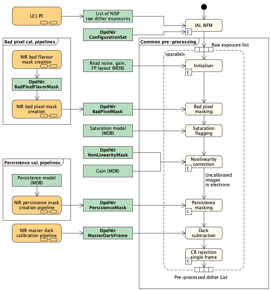
Figure 1: NIR PF pre-processing. Input products are shown as green boxes on the left. Some of them are taken from the MDB, while other products are generated by dedicated processing pipelines represented as orange boxes.

3.1.1 Detector baseline

The detector baseline is a pedestal set to ensure positive values in the analogue-to-digital converter (ADC) output, as well as an optimal use of the detectors’ dynamic range in a linear manner. The baseline PE does not manipulate or calibrate NIR Level 1 (LE 1) data. Instead, based on the results obtained from the NISP on-ground test campaign (Barbier et al. 2018, Kubik et al., in prep.), it is used to validate the correct baseline setting. This is essential for guaranteeing accurate signal measurements, that is to operate the detectors within the ADC linear range.

After an initial setting done during Euclid’s commissioning phase (Cogato et al. 2024), the detectors baseline was verified at a nominal operational temperature of 94 K. To this end, 64 consecutive dark exposures were acquired with the MACC(1,16,1) mode (Kubik et al. 2016), that is a single group of 16 co-added frames. From these, the baseline map is estimated as the median signal over the image stack after correcting raw images for reference pixel drift (Kubik et al. 2014; Medinaceli et al. 2020, Kubik et al., in prep.).

The baseline maps are verified by comparison with the ground-based differential nonlinearity (DNL) range for reference and science pixel distributions. The baseline maps are stored in the Euclid archive and the DNL outliers are included in the bad-pixel map (see Sect. 3.1.3 and Fig. 2). As a by-product of this PE, the so-called kTC noise map is estimated by computing the signal standard deviation across the dark image stack (Kubik et al., in prep.). The kTC noise originates from the thermal fluctuations in the pixels capacitance during reset.

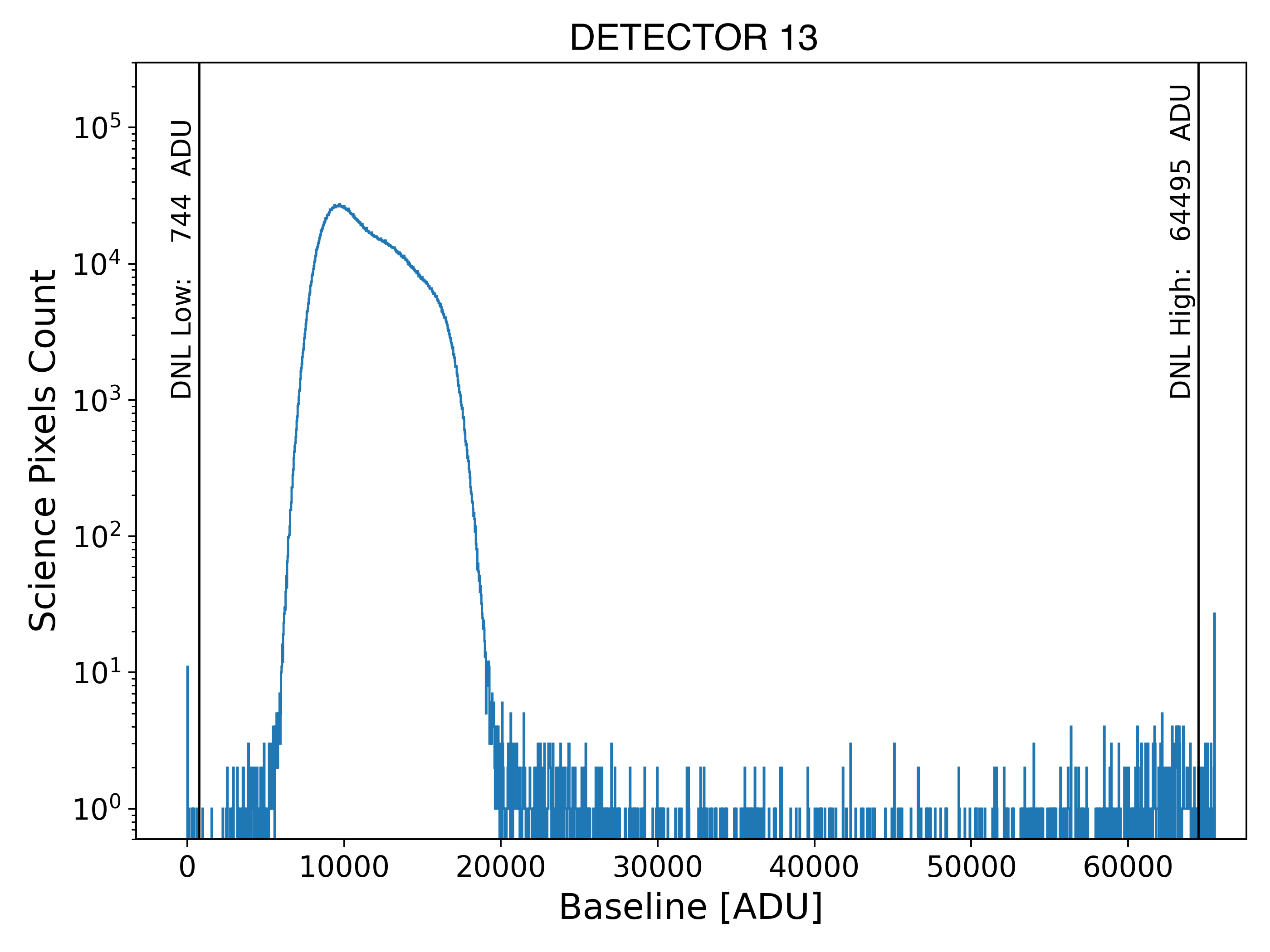
Figure 2: Example of the science pixels’ baseline distribution for one of the detectors (DET13) measured during PV. Solid black vertical lines show the boundary of the DNL range defined during the ground-test campaign.

3.1.2 Unstable channels

Euclid H2RGs detectors operate in 32-output readout mode. This means that they are divided into 32 channels of 64 2048-pixel columns, and the channels are read out in parallel. Over the 16 detectors, a few channels show a top-bottom gradient, with various amplitudes and frequency of occurrence. This effect was identified on the ground for some channels, but the set of channels affected by this has changed slightly in flight. Two types of gradients have been identified.

First, most cases show a linear slope from top to bottom. Those cases can be detected and corrected using the reference pixels. Each detector channel has four rows of reference pixels at the top and at the bottom of the array. Reference pixels are not connected to the detector photodiodes and they allow subtraction of the frame-to-frame bias and temperature drift (Kubik et al., in prep.). In flight we have access to all frames at the top and bottom of two reference lines, used to compute a gradient from top to bottom and thus identify unstable channels. The amplitude of this slope can be used to compute a correction. This procedure is currently applied to the 6 channels for which the amplitude can be detected with high significance above the noise floor.

Second, other cases show a quadratic slope, where the top and bottom parts of all columns of the channel are brighter while the middle part is darker. This happens usually with the longer integration times of the MACC(15,16,11) spectroscopic exposures, and cannot be detected with reference pixels because they do not detect the lower values near the channel’s mid-point.

3.1.3 Bad-pixel identification and masking

We use ground test data of the H2RGs as the primary resource to identify bad pixels for Q1. These pre-launch evaluations of the pixel performance were taken over three main campaigns: acceptance testing and ranking at the NASA Goddard Space Flight Center’s Detector Characterisation Laboratory (DCL) in 2016; individual component tests in 2019 at the CNRS-IN2P3 Center for Particle Physics in Marseille (CPPM); and fully-integrated flight-module tests in space-like conditions (thermal vacuum and thermal balance, or TBTV) at Laboratoire d’Astrophysique de Marseille (LAM) in 2019–2020. The TBTV and final pre-launch payload module (PLM) tests with NISP integrated into the telescope are summarised in Medinaceli et al. (2022).

In addition, baseline calibration measurements were taken during commissioning and incorporated into the bad-pixel maps for NIR PF (see Sect. 3.1.3). Calibration observations obtained during the PV Phase are not reflected in Q1.

Pixels revealed to be permanently inoperable for science, or exhibiting noteworthy performance characteristics that may affect operability, are contained in calibration data products for the NISP Level 2 pipeline. A map has been created for each pixel condition (or ‘flavour’) by detector, assigned a 16-bit unsigned integer 2ⁿ, $n$ ¿ 1, and merged into a master bad-pixel mask (BPM) that can be used by NIR PF. The BPM application updates the data quality (DQ) layer accompanying each of the 16 science frames, with no distinction between imaging and spectroscopy modes. DQ values are the bit-wise sum for pixels of more than one flavour.

The BPM is not restricted to scientifically inoperable pixels. To distinguish unusable from informational flavours, the bit 0 is reserved for the unusable cases. This ‘INVALID’ bit is summed only once, even when a pixel has been flagged with more than one fatal condition, as is often the case. Thus INVALID pixels will always have an odd DQ value. Further details, including bit assignments, can be found in Morris & Kubik (2022) and Euclid Collaboration (2025). Statistics for the non-transient – that is static – pixel masks are summarised in Table 1, and in the following we review the most important flags.

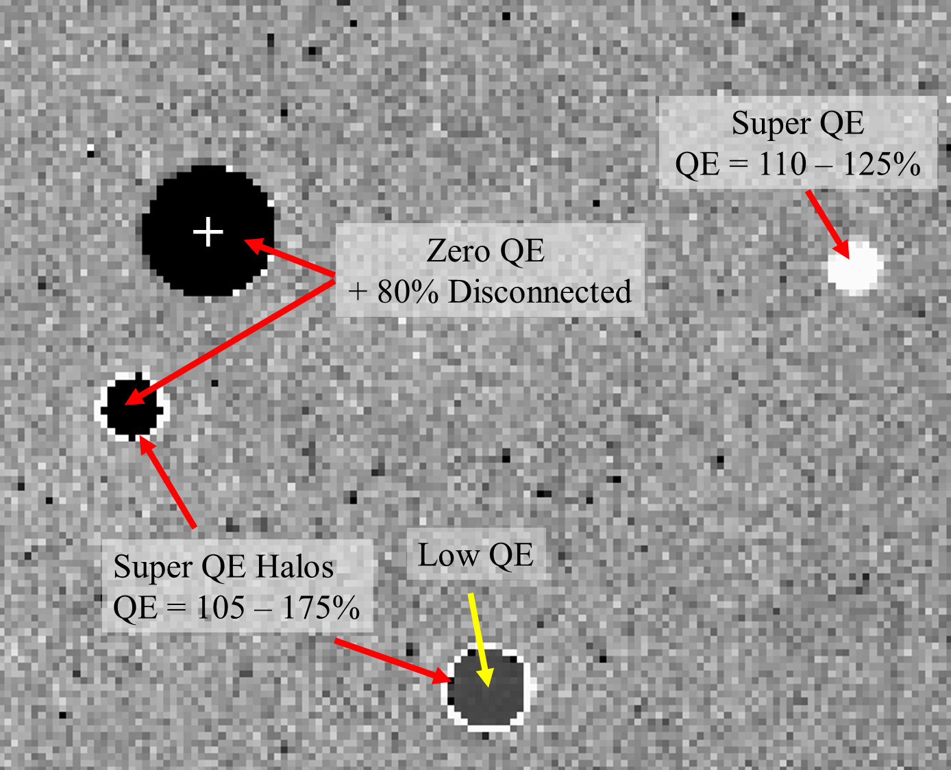
Figure 3: Representative flagged QE ‘flavours’ in Q1, detector 44 in this example. Grey background pixels are in the range of 5–100% QE. Zero and Super QE pixels are INVALID in NIR PF, while Low QE pixels are flagged for monitoring. Super QE pixels often appear as a 1-pixel wide bright halo around groups of disconnected pixels, although the largest group in this example does not exhibit a halo – the QEs of neighbouring pixels are within the nominal range to within the 5% measurement uncertainty. For reference, ‘+’ indicates pixel [$x$,$y$] = [1458,1336] in Level 2 2040 $\times$ 2040 array coordinates. The labelled QE ranges are wavelength-averaged.

Invalid flags. Pixels in Q1 data are flagged invalid if: (i) they are unresponsive due to disconnection from the readout-integrated circuit; (ii) their quantum efficiency is very low or poorly known; and (iii) if their baseline after bias reset is outside the photometrically calibratable range.

DISCONNECTED

pixels have absent or non-working indium bumps for connection to the photosensitive diodes. They terminate at the capacitor and have no detectable photo-sensitivity. Some positive residual charge is generally present for them in the readout electronics. Measurements were done under specific laboratory conditions at ambient room temperature and thus could not be repeated in the same fashion after launch.

ZERO QUANTUM EFFICIENCY

pixels were identified during detector qualification tests at the DCL. Such pixels are flagged when the measured quantum efficiency (QE) is less than 5% (corresponding to the low-end measurement uncertainty) averaged over wavelengths $920\,{\rm nm}\leq\lambda\leq 1120\,{\rm nm}$. Most disconnected pixels have zero QE.

SUPER QE

pixels have wavelength-averaged QEs greater than 110%. Such pixels generally surround clusters of disconnected pixels, creating a bright, 1-pixel wide halo under illumination as photocurrent flows from the disconnected pixels to the nearest photosensitive neighbours with usable well depths. Figure 3 shows an example. Thus the measured QEs become artificially high – reaching as much as 200% in some cases – and unrecoverable.

BAD BASELINE

pixels have baselines that are either too high or too low after bias reset and fall into a range of excessive kTC noise. Because the ground-based baseline data were obtained at a lower temperature than where the NISP FPA operates on orbit by about 6 K, the baselines were remeasured during commissioning (see Sect. 3.1.1) and updated in the BPM. This is the only flavour that has been updated with in-flight data for the Q1 release.

Informational flags. Certain flags have been reserved for monitoring purposes. In Q1, hot and low QE pixels are tracked but are not set to INVALID, pending further evaluation of their operability for science with flight data.

HOT

pixels have been defined differently in the literature by the sensor-chip manufacturers and the intended application. For NISP the signal of a hot pixel is 3 $\sigma$ above the most probable value of the detector’s measured dark current. Pixels with elevated dark currents are not necessarily INVALID, as long as the unilluminated output signal is stable and below the saturation limit. Hot pixels were identified from ground-based dark current measurements, and are updated and checked for stability in flatfield measurements taken during PV and in the routine phase with the LEDs over a range of fluences.

LOW QE

pixels are flagged when nominal requirements set by NASA are not met to within the 5% RMS uncertainty for measurements at $920\,{\rm nm}\leq\lambda\leq 2020\,{\rm nm}$,

• QE $\geq$ 74% for $\lambda\in[1120,2020]$ nm, and

• $\mathrm{QE}\geq\left[64+(\lambda/\mathrm{nm}-920)/20\right]\%$ for $\lambda\in[920;1120]$ nm.

The data from such pixels are expected to be calibratable, pending further evaluation with flight data, but will generally exhibit reduced signal-to-noise levels compared to pixels with nominal QE.

Table 1: NISP Detector Non-Transient DQ Flags and Dark Currents in Q1

DetID	Invalid pixels				Informational		Dark MPV
	DISCONN	ZEROQE	SUPERQE	BADBASE	LOWQE	HOT	Photo	Spectro
11	135	747	290	27	591	630	0.007	0.016
12	3223	5399	7038	25	953	3056	0.000	0.015
13	589	1261	551	74	219	644	0.014	0.024
14	252	1858	579	183	597	2794	0.018	0.029
21	313	1275	16	171	292	1060	0.009	0.012
22	2580	3510	1313	2127	331	1645	0.003	0.014
23	1512	1992	2373	75	605	754	0.009	0.015
24	146	698	302	15	216	420	0.000	0.010
31	1420	2054	992	72	725	1743	0.004	0.014
32	269	895	307	76	420	1161	0.004	0.013
33	262	1288	644	95	402	1535	0.003	0.014
34	970	2072	249	105	390	1159	0.002	0.013
41	198	1858	339	63	585	631	0.000	0.009
42	334	847	404	143	390	807	0.006	0.018
43	222	1129	401	17	278	369	0.007	0.017
44	255	7420	558	707	1542	4076	0.010	0.017

3.1.4 Nonlinearity correction

Nonlinearity in H2RGs is primarily caused by the behaviour of the photodiode’s junction capacitance. As charge accumulates in a pixel during exposure, the depletion region of the photodiode narrows, leading to an increase in junction capacitance. This change affects the conversion of accumulated charge to voltage, causing deviations from the ideal linear response. Additionally, other components in the signal chain, such as the source follower in the readout integrated circuit and the ADC process, can introduce further nonlinearities. These combined effects result in a nonlinear relationship between the incident photon flux and the measured signal, with the nonlinearity becoming increasingly pronounced as the flux level rises, independent of wavelength (see e.g., Plazas et al. 2017; Barbier et al. 2018).

We calibrate the pixel-level response and nonlinearity with custom-designed LEDs (Euclid Collaboration: Hormuth et al. 2024; Euclid Collaboration: Jahnke et al. 2024). Each LED has a narrow emission spectrum and can illuminate the FPA with varying fluxes. For nonlinearity calibration – conducted on-ground and in-flight – two key measurements are required: the fitted slope image (Kubik et al. 2016) that represents the nonlinear response, and the individual MACC group images that are used to approximate the linear flux $F_{\text{Linear}}$ (e.g., Vacca et al. 2004). For both photometry and spectroscopy readout modes, MACC(4,16,4) and MACC(15,16,11) respectively, five fluence levels are selected to span the dynamic range expected for each mode, accounting for their different exposure times. These measurements are then combined to derive nonlinearity calibration coefficients for each pixel.

The linear flux estimate, $F_{\text{Linear}}$, is derived by modelling the pixel response across various fluence levels using orthonormal polynomials. The first term of this model provides an approximation of the linear flux, as fully described in Kubik et al. (in prep.). Orthonormal polynomials were chosen for their practical advantages, including computational efficiency and manageable memory usage, and this approach has been successfully adopted for correcting H2RGs at several facilities. In the long term, more sophisticated models, such as a principal-component analysis, will be evaluated to enhance nonlinearity corrections (see also Rauscher et al. 2019). Before fitting, the ramps are corrected for reference pixels using sliding windows of four pixels. To optimise memory and CPU usage, the ramps, observed multiple times at each fluence level, are averaged for each run. Additionally, frames exceeding $60\,000$ ADU are rejected to avoid saturation effects.

Following preprocessing, the nonlinearity per pixel is expressed as a 4th-degree polynomial relationship between the estimate of the linearised flux $F_{\text{Linear}}$ and the measured nonlinear flux $F_{\text{Nonlinear}}$

$$F_{\text{Linear}}=\sum_{k=0,4}a_{k}F_{\text{Nonlinear}}^{k}\,.$$ (1)

The degree of the polynomial is constrained by the number of available fitting flux levels, and for consistency purposes we enforce the linear flux to be zero for a zero nonlinear flux.

Fitting these polynomials to the thermal vacuum (TV1) calibration data, we measured the nonlinearity coefficients and their covariances, which are subsequently used in the NIR PF nonlinearity correction for Q1. The validity range is dictated by the dynamic range covered by the LED fluences (1000 ADU to 30 000 ADU), below which nonlinearity effects are minimal and above which corrections are applied by linearly extending the polynomial fit rather than using the higher-order coefficients. It should be noted that the values above already include baseline removal. Considering the baseline level shown in Fig. 2, we expect saturation to occur between 40 000 and 50 000 ADU for most of the pixels. For the first data release DR1, expected in October 2026, additional fluences from PV and calibration observations are expected to enlarge the validity range. The correction step also incorporates gain conversion, and a flagging of pixels where the fit is unreliable. In addition, pixels whose signal exceeds the saturation threshold defined from the ground-test campaign are identified by this PE and flagged using both SATURATION and INVALID bits.

3.1.5 Persistence masking

Persistence model - calibration product from ground characterisation

Charge persistence is the effect of electrons being trapped in detector defects, and being released again on time scales of minutes and hours (see e.g., Smith et al. 2008; Leisenring et al. 2016; Tulloch 2018). This leads to ghost images of previous exposures in subsequent exposures, affecting photometric and spectroscopic measurements. NIR PF masks persistence using an effective persistence model calibrated on ground-characterisation data (cf. Kubik et al., in prep., Kubik et al. 2024) for illuminations below saturation.

During the TV1 characterisation campaign, a standard protocol for persistence calibration was used. It consisted of a set of flat field exposures of 87 s with increasing fluences. Each of the flat exposures was followed by a dark exposure of 430 s.

The signal in the flat fields was estimated by the linear fit to the first 50 frames of the ramp. The subsequent frames were discarded from the fit to avoid nonlinearity effects. Dark exposures were used to measure the persistence signal accumulated in exposure times that match those in the ROS (Euclid Collaboration: Jahnke et al. 2024). The first 26 or 175 frames of the dark exposures were discarded to account for the persistence decay during the dither time or slew time, respectively, between two consecutive exposures in the reference observing sequence (ROS). The remaining frames were fitted using the on-board signal estimator of Kubik et al. (2016). The photometric readout mode, MACC(4,16,4), was used to estimate persistence in photometric exposures. To estimate persistence in spectroscopic exposures MACC(7,16,1) with 16 frames per group was used, that was the maximum possible, since the dark ramps during TV1 persistence testing were too short to compute persistence in the spectroscopic exposure time. In each case, the obtained slopes were multiplied by the corresponding total exposure time, converted to electrons using the gain per channel map. The dark-current was also subtracted . All coefficients are estimated per pixel, since the persistence amplitudes have high spatial variability (Kubik et al. 2024).

The calibrated effective persistence model yields the persistence charge $Q_{\mathrm{P}}$ as a function of the previous illumination amplitude $S$ using the expression

$$Q_{\mathrm{P}}(S)=\left(\alpha+\beta S\right)\left(1-\mathrm{e}^{-S/\gamma}\right)\,.$$ (2)

Separate sets of coefficients $\alpha,\beta,and\gamma$ are needed to describe persistence in photometric and spectroscopic exposures, due to their different exposure times.

This model is effective in the sense that the persistence decay during one exposure is built in the coefficients of the model, but there is no explicit time dependence of the persistence decay. Other shortcomings of this model are that it does not take into account the superposition of persistence from multiple bright exposures, and it does not account for charge trapping, resulting in a potential lack of signal for bright sources on pixels that have previously seen a low-background exposure.

Persistence masking procedure

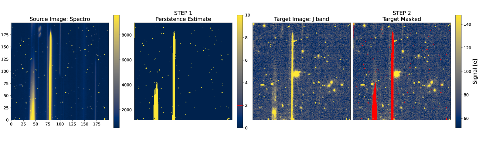
Figure 4: Persistence masking scheme. In the first step, the persistence estimate is calculated using the persistence model applied to prior exposures (source images) for each target exposure. In the second step, the persistence estimates are thresholded to identify and mask pixels where the persistence charge exceeds 2 e^- (indicated in red in the right image). Typically, the percentage of masked pixels does not exceed 2%.

There are two separate steps to mask persistence, presented schematically in Fig. 4. The first step consists of the estimation of persistence charge contributing to any of the NISP scientific exposures. It is a separate pipeline executed before the proper NIR data reduction, in which for each exposure the persistence charge originating from previous images is estimated and stored as a separate product (persistence estimate image). Taking into account the limitations of the effective model, for each photometric exposure only the persistence charge from one previous spectroscopic image is computed. To account for the persistence decay over one dither, the model computes $Q_{\mathrm{P}}$ using the calibrated set of parameters in Eq. 2 – this is the prediction of the persistence from a spectroscopic image to the $J_{\scriptscriptstyle\rm E}$-band image – and a rescaling factor is applied to estimate the persistence contribution to the $H_{\scriptscriptstyle\rm E}$- and $Y_{\scriptscriptstyle\rm E}$-band images taken next in time. We note that for Q1 processing the persistence contribution originating from photometric exposures is not taken into account because, given the Euclid ROS, that would result in masking most of the bright sources. A more accurate model to allow for a correction procedure is being developed. Likewise, the computation and masking of persistence in spectroscopic exposures is deactivated for Q1.

The second step is the persistence masking executed during the NIR scientific pipeline. In this task, for each photometric exposure, the corresponding persistence image is analysed. If the persistence charge amplitude in a pixel exceeds 2 e^-, then a PERSIST and INVALID flag is raised in the DQ layer of the science exposure (Appendix B). For some pixels the persistence coefficients could not be calibrated, and consequently the persistence charge could not be estimated. In that case, the PERMODFAIL flag is raised in the DQ layer of the corresponding image.

3.1.6 Dark current

The master dark frames were updated from ground-based (TBTV) characterisation (Kubik et al., in prep.) with two blocks of measurements taken during PV at 87 s and 548 s integration times, corresponding to the imaging and spectroscopic science modes, respectively. We refer to these as photo- and spectro-darks. The darks are taken after a sufficiently long pause to allow for the decay of previously built-up persistence charge. With the filter wheel in its closed position, the dependence of the measured dark current is thus purely on exposure time. Sets of 500 photo- and 100 spectro-darks were acquired to obtain a sufficient signal-to-noise ratio (S/N). The PE that generates the master dark uses an iterative procedure to reduce the impact of spurious detections from the active space weather near the maximum of the 25th Solar cycle.

To estimate pixel noise performances, the median absolute deviation (MAD) is measured on the array of pixel values $a_{i}$ (the 0th axis of the datacube of slope images), where the MAD is defined as the median (med) of $\left|a-{\rm{med(}}a{\rm{)}}\right|/c$. The normalisation constant is $c\approx 0.6745$. The MAD is used to set the noise threshold, outside of which values are masked from the array $a$; that is $a>$ med($a$) $\pm$ $n_{\rm MAD}\times\,$MAD are masked. However, They are not removed since this is only a noise-performance-selection step needed for the subsequent dark detection. Simulations using ground-based dark currents including readout noise and varied cosmic ray (CR) fluences in the Earth-Sun L2 orbit set the optimum value of $n_{\rm MAD}$ at 3.0.

After masking to the MAD-based threshold, the median of $a$ is taken again, and the result is evaluated for detection of the dark current above the S/N given by the two conditions $\left|{\rm{med(}}a{\rm{)}}\right|\leq$ RMS/$\sqrt{N_{\rm{fr}}}$ and RMS/$\sqrt{N_{\rm{fr}}}\leq$ 0.3$\,\times\,\sqrt{480/N_{\rm{fr}}}$ , where RMS is the standard deviation and $N_{\rm{fr}}$ is the number of measurements in each pixel meeting its initial threshold; for example, $N_{\rm{fr}}\leq 500$ in the case of the PV photo-darks. The final median dark currents and their variances comprise the master dark product, along with a DQ flag set for pixels whose dark currents could not be detected to within the two noise conditions. This flag, NODARKDET, is informational and does not necessarily represent an invalid condition. This is because some pixels in H2RGs have such a low dark current that the slopes computed are dominated by the readout noise, and for example, also a floor of weak CR-induced signal not completely compensated by the masking steps – an issue demonstrated with simulations. Strictly speaking, however, such pixels cannot be distinguished from those with sufficiently high noise arising from multiple sources that their dark currents are hidden from detection. Thus, for all flagged pixels the dark current is set to zero and these are excluded from the detector dark-current performance statistics; see Table 1 for the most probable values of the dark current applicable to Q1.

3.1.7 Cosmic-ray identification

Single-frame photometric mode

The first step in the identification of CRs in the NISP photometric data is performed by the module NIR_CrRejectionSingleFrame. This module utilises the LAcosmic algorithm (van Dokkum 2001) to locate CRs in single photometric exposures using Laplacian edge detection. The algorithm has several input parameters that strongly depend on the instrument and conditions of the observations. A balance has to be found between identifying a large fraction of the CRs without masking real (point) sources. This is especially important for NISP, which strongly undersamples the PSF (Euclid Collaboration: Jahnke et al. 2024). For each of the three NISP filters, the optimal set of input parameters were found based on simulated images, for which the ground truth is known. In this tuning, the priority was to avoid masking real objects, since CRs not identified in this module can be picked up by the multi-frame CR-rejection module (see below). The efficiency of this module is higher for the redder filter $H_{\scriptscriptstyle\rm E}$ compared to the bluest filter $Y_{\scriptscriptstyle\rm E}$, since undersampling is stronger in the bluer passband.

Pixels identified by LAcosmic as CRs are masked by adding the flags COSMIC (bit 16) and INVALID (bit 0) to the DQ layer. We also mask all eight neighbouring pixels to account for inter-pixel capacitance (IPC) that spreads charge from a pixel to its neighbors, which then also need to be masked in the case of a CR. For details about IPC see Le Graët et al. (2022) and Euclid Collaboration: Jahnke et al. (2024).

Multi-frame photometric mode

This is the second step in identifying and flagging CRs, using information from all available dithers simultaneously and implemented in the NIR_CrRejectionMultiFrame module. This task requires precise astrometric calibration (see Sect. 3.2.7). Each position in the sky, corresponding to a pixel on the array, is observed with $n$ dithers. In the EWS, the ROS dither pattern results in fractions of 1%, 8%, 40%, and 42% for $n=1$ to 4, respectively (see table 2 in Euclid Collaboration: Scaramella et al. 2022). We use pull-clipping for outlier detection that is robust on such small samples ($n\geq 3$ unflagged data points). More specifically, we reject pixels with the pull $p_{i}\geq 10$, where $p_{i}$ is defined as

$$p_{i}=\frac{(x_{i}-\bar{x_{i}})}{\sqrt{\sigma_{i}^{2}-\bar{\sigma}_{i}^{2}}}\,.$$ (3)

Here, $x_{i}$ and $\sigma_{i}$ are the respective flux and measurement error of dither $i$, and $\bar{x}_{i}$ and $\bar{\sigma}_{i}$ are the inverse-variance weighted average and the associated sample error without point $i$. We note that for the monthly visits of Euclid’s self-calibration field (see Sect. 4.2.3 in Euclid Collaboration: Mellier et al. 2024) near the North Ecliptic Pole (NEP) we have coverage of up to $n=76$, and that for $n<3$ we fall back to the single-frame mode explained above.

To counter false positive CR detections – for example stars erroneously identified as CRs – we compute the sum of pixel values in the 3 $\times$ 3 pixel region around the candidate CR. The same sum is computed for the other dithers. The CR-detection is rejected if the sums agree to within 3%. All detected CRs are flagged in the DQ layer.

For testing purposes, or in the case of a malfunction in specific scenarios, standard sigma-clipping or Grubb’s test can be enabled in NIR PF. This estimates the $z$-score,

$$z_{i}=\frac{(x_{i}-\bar{x})}{s}\,,$$ (4)

where $\bar{x}$ and $s$ are the sample mean and standard deviation, respectively. For small $n$, this method has the disadvantages that it includes outliers in the sample estimates, and that it does not fully account for individual measurement errors $\sigma_{i}$. A comparison with the pull-statistic for small sample sizes is given in Copin (2022). Since $n\leq 4$ for the EWS, we adopted the pull clipping as default statistic for the NIR PF.

Single-frame spectroscopic mode

Each MACC(15,16,11) grism exposure is associated with an 8-bit image of quality factors containing the $\chi^{2}$-statistics of the on-board slope-fit (see Kubik et al. 2016). The current version of the SIR_CrRejectionSingleFrame module in NIR PF uses this $\chi^{2}$ value to identify CRs. Figure 5 shows the $\chi^{2}$ distribution for one detector plotted together with the probability density function (PDF) with degree of freedom ${\rm DOF}=13$. According to Kubik et al. (2016), $N_{\rm dof}=n_{\rm g}-2$, where $n_{\rm g}=15$ is the number of groups in the nominal MACC spectro-mode. Figure 5 also indicates the threshold (50 counts) to detect bad pixels. From simulated data we found that the $\chi^{2}$ implementation identifies at least 99% of the CRs.

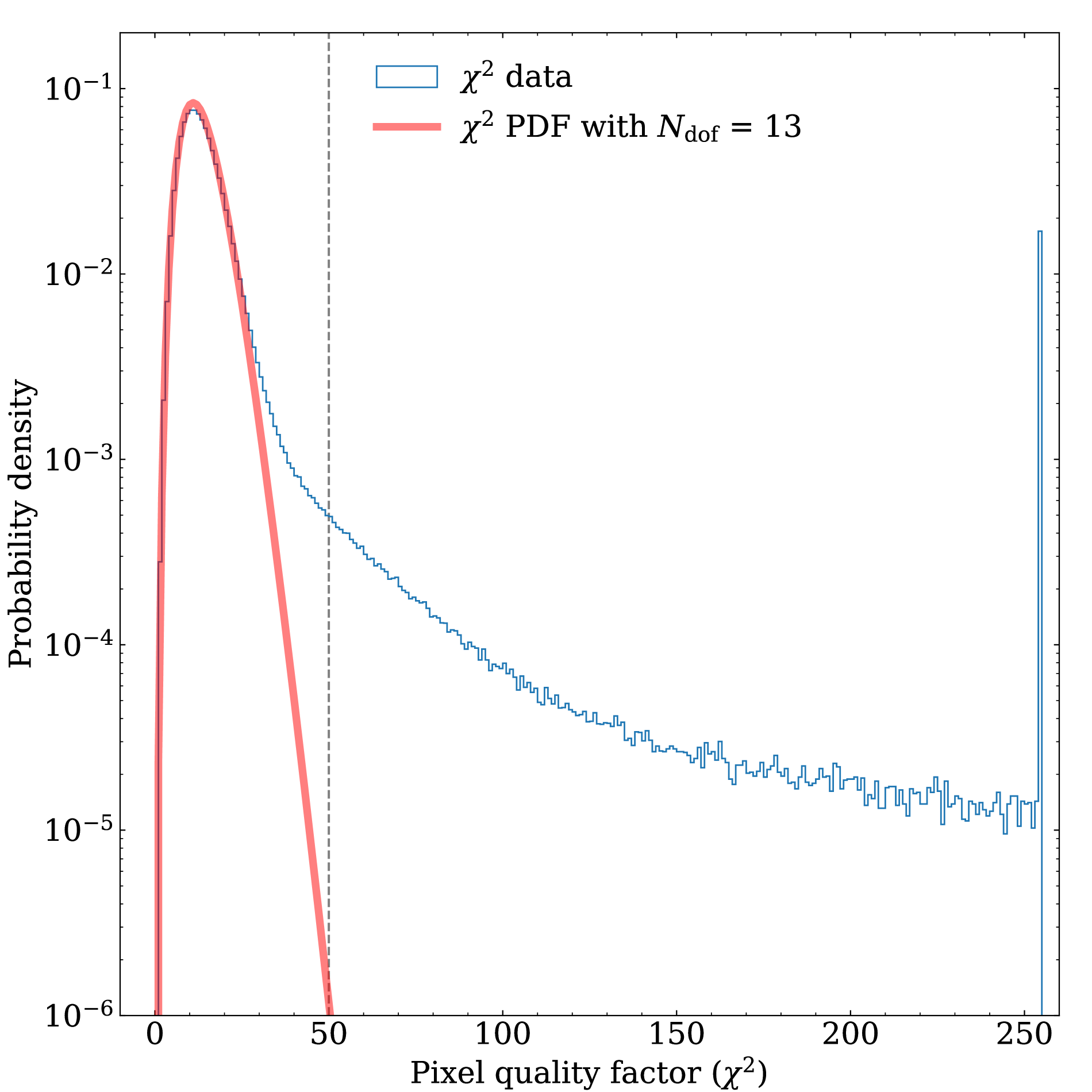
Figure 5: Comparison between the PDF of the pixel quality factors ($\chi^{2}$) for a spectroscopic MACC(15,16,11) exposure for one of the NISP detectors (blue histogram), and the PDF calculated for a $\chi^{2}$ distribution with ${N_{\rm dof}}=13$ (red line). The threshold $\chi^{2}=50$ (dashed vertical line) distinguishes good- from bad-quality pixels. The $\chi^{2}$ value is encoded on-board as an 8-bit integer and thus has an upper limit of 255. Hence, the last bin corresponding to $\chi^{2}=255$ includes not only CRs, but all other pixels with a poor slope fit, such as bad pixels.

Alternatively to using $\chi^{2}$, the single-frame spectroscopic mode can also run LAcosmic as implemented for photometry in NIR_CrRejectionSingleFrame, albeit with different configuration parameters. We find that combining LAcosmic with the $\chi^{2}$ approach does not increase the completeness fraction of detected CRs, and therefore SIR_CrRejectionSingleFrame defaults to the $\chi^{2}$ method alone.

3.2 Astrometric and photometric calibration of NISP images

In this section we describe the PEs in NIR PF that derive the astrometric and photometric calibrations (Fig. 6).

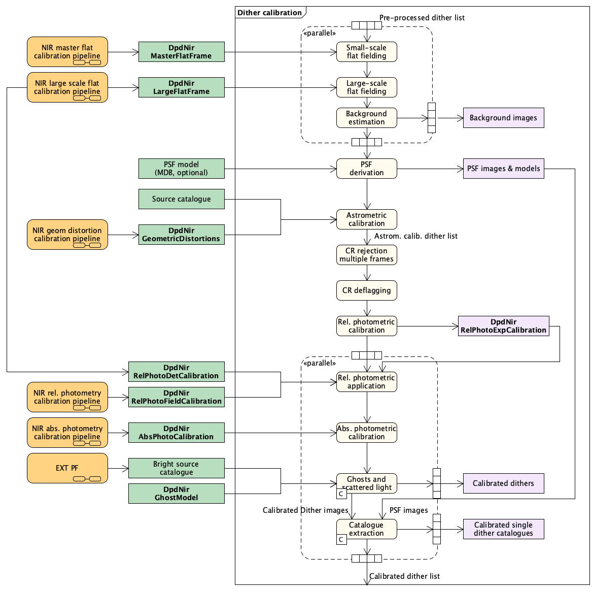
Figure 6: NIR PF astrometric and photometric calibration PEs. Input products are shown as green boxes on the left. Some of them are taken from the MDB, while other products are generated by dedicated processing pipelines represented as orange boxes.

3.2.1 PRNU correction using LED flat fields

The detectors’ pixel-response non-uniformity (PRNU) is corrected with flat fields. The ideal PRNU correction would be given by the relative detector response to a uniform illumination from a continuum white-light source. NISP, however, uses LEDs with a near-monochromatic spectral energy distribution (SED) in the near-infrared calibration unit (NI-CU; Euclid Collaboration: Hormuth et al. 2024). NI-CU incorporates five LEDs A to E, ordered by ascending central wavelengths of their spectra (Fig. 7). It illuminates the FPA directly from a small off-axis angle, without passing through a filter (see section 2.2. of Euclid Collaboration: Hormuth et al. 2024, for more details). The spatial illumination approximately follows a Lambertian cosine profile (Euclid Collaboration: Hormuth et al. 2024).

A single LED flat alone thus does not represent an ideal PRNU correction. Therefore, after going through all pre-processing steps listed in Sect. 3.1, we reconstruct filter-dependent flats from the individual LED flats. Denoting the LED flat as ${\rm FLAT_{\rm LED}}(\mathbf{x})$, with $\mathbf{x}$ being the pixel position, we compute the filter-dependent flat as

$${\rm FLAT_{Filter}}(\mathbf{x})={\rm FLAT_{\rm LED}}(\mathbf{x})\;P(\mathbf{x})\;.$$ (5)

Here,

$$P(\mathbf{x})=\frac{\int_{\lambda_{1}}^{\lambda_{2}}\mathrm{QE}(\lambda,\mathbf{x})\;T(\lambda,\mathbf{x})\;{\rm d}\lambda}{\int_{\lambda_{3}}^{\lambda_{4}}\mathrm{QE}(\lambda,\mathbf{x})\;{\rm d}\lambda}$$ (6)

propagates the LED’s SED across the detector’s QE to reconstruct a broad-band flat from a near-monochromatic light source. $T(\lambda,\mathbf{x})$ is the filter transmission curve, $[\lambda_{1},\lambda_{2}]$ is the passband of the filter, and $[\lambda_{3},\lambda_{4}]$ is a representative wavelength coverage of the LED spectrum. Notably, due to the LEDs’ narrow SED, $P$ is independent of the LED spectrum. The mathematical derivation of Eqs. 5 and 6 is given in Appendix A. The data for QE and $T(\lambda)$ used for the Q1 data processing were measured on the ground (Euclid Collaboration: Schirmer et al. 2022). We note that $P$ is in principle time-dependent over mission-duration due to radiation damage and molecular contamination (Euclid Collaboration: Schirmer et al. 2023), but in the context of the singular Q1 observations this dependence can be neglected.

Of the five LEDs available, only LEDs B to D are used to construct the broad-band flats. Given the mutual wavelength coverages, we use LED B for filter $Y_{\scriptscriptstyle\rm E}$, C for $J_{\scriptscriptstyle\rm E}$, and D for $H_{\scriptscriptstyle\rm E}$ in Eq. 5. In principle, several LEDs can be combined to reduce uncertainties from the propagator $P$, but the LED-flat S/N is so high that there is currently no need to do so, mainly because the QE curves are very flat across the passbands, and the S/N in the QE maps themselves is also very high.

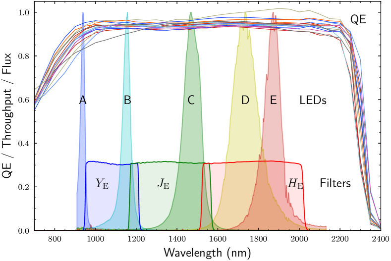
Figure 7: Comparison of the average QE curves of the 16 NISP detectors, the normalised SEDs of the LEDs, and the $Y_{\scriptscriptstyle\rm E}$, $J_{\scriptscriptstyle\rm E}$, and $H_{\scriptscriptstyle\rm E}$ passbands (reduced by a factor 3 in height to avoid cluttering near the top of the plot).

Each of the three filter flats is computed from 30 LED flats. In addition to the bad pixels identified by the pre-processing steps, the filter flats require further masking. The first type is vignetting from a baffle near the FPA, which affects the edges of detectors 11, 14, 24, 34, and 44 for LED frames (see section 2.3. of Euclid Collaboration: Hormuth et al. 2024). Pixels in the vignetting regions are flagged as VIGNET and their values are set to 1.0 in the master flat. The second type of pixels masked are ‘flower’ pixels, which typically present a cross-shaped pattern with a faint core (‘flower centre’) and bright adjacent pixels (‘flower petals’). The same type is found in James Webb Space Telescope (JWST) images, where they are referred to as ‘open’ and ‘adjacent to open’ pixels (Rauscher et al. 2014). Flower pixels are masked as FLOWER and INVALID. We detect these pixels in the flat exposures using a Laplacian kernel. Finally, pixels with values that deviate from the median of the 30 frames by over 50% are flagged as FLATLH, indicating too-low or too-high values without further discrimination.

The master flats of the three NISP bands used for the Q1 processing are shown in Fig. 8. The PRNU correction is done by dividing the science frames by the master flat, without prior removal of NI-CU’s Lambertian illumination profile.

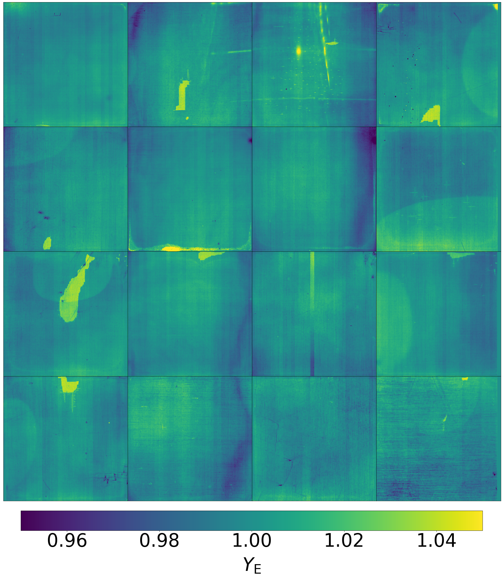
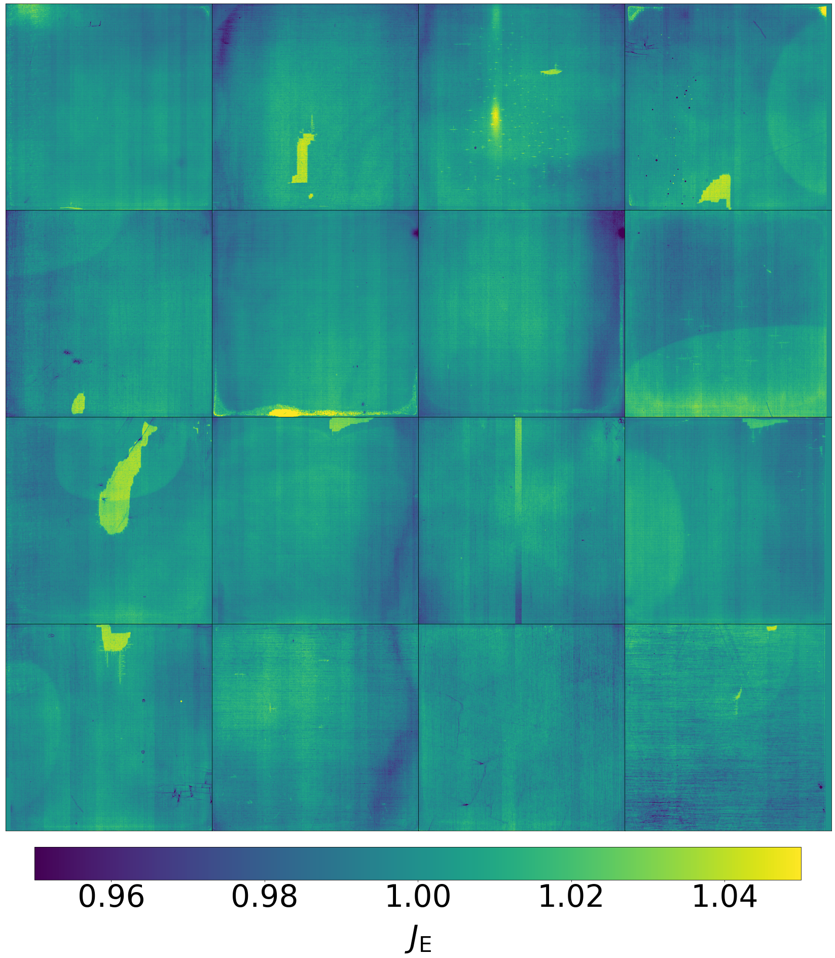
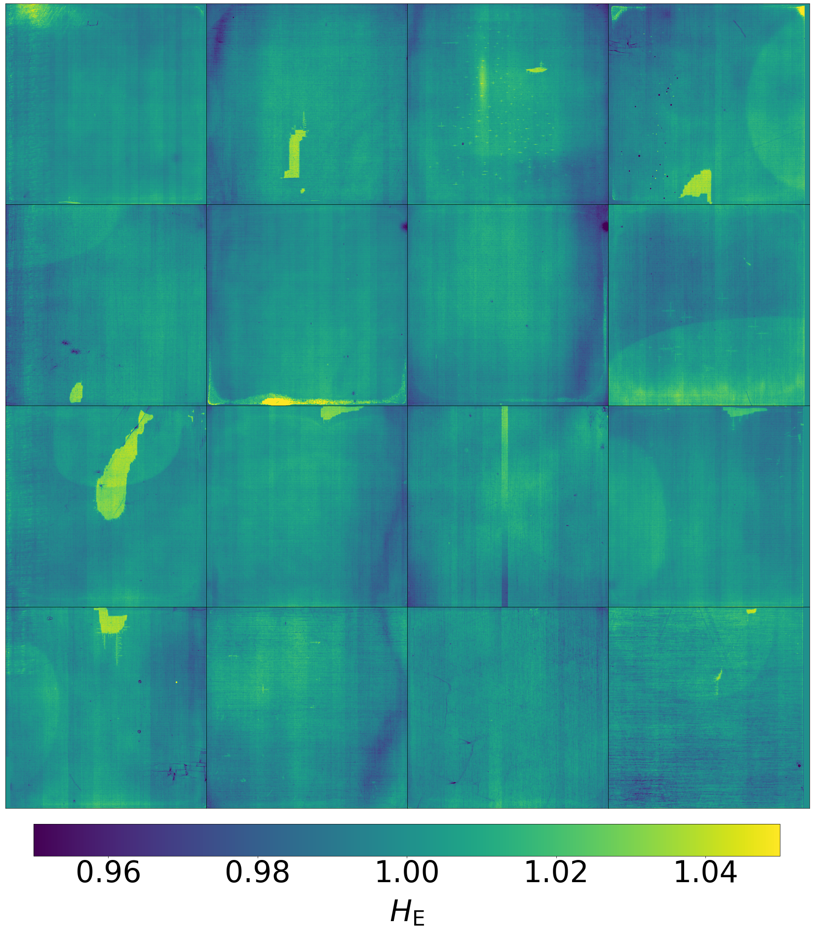
Figure 8: Master PRNU flats for Euclid $Y_{\scriptscriptstyle\rm E}$, $J_{\scriptscriptstyle\rm E}$, and $H_{\scriptscriptstyle\rm E}$ bands used for the processing of Q1 images. The uniform QE is evident from these images.

3.2.2 Large-scale illumination correction

The LED illumination profile is not removed prior to PRNU correction (Sect. 3.2.1), introducing a multiplicative flux change across the PRNU-corrected images on the order of 10%. While Euclid’s telescopic beam is free of vignetting, non-uniformities in the illumination of the FPA still arise. For example due to the cosine-fourth-power-law of illumination (Reiss 1945), modified by Euclid’s off-axis optical design (Euclid Collaboration: Mellier et al. 2024), and by angle-of-incidence dependencies of the mirror reflectances. Jointly, these are expected to be on the order of 1–2%.

A photometric flat is required to correct for these non-uniformities on scales larger than about 100 pixels; below that scale, the LED flats can be assumed to be uniform apart from PRNU. The photometric flat, or large-scale flat, is computed by measuring how the fluxes of stars change when they move to different FPA locations in the 76 widely-dithered exposures of Euclid’s self-calibration field. In NIR PF, the NIR_SelfCalib processing element performs this computation, and also applies it to the science images. This also includes a determination of the relative, average detector-to-detector sensitivity variations.

We note that the internal computations are performed in magnitudes, not in linear fluxes. Specifically, we consider observations of the same source in different locations on the FPA, and assume the observed magnitude is the sum of three contributions: the source actual apparent magnitude; an additional term due to the detector non-flat sensitivity; and a third term due to the detector average sensitivity,

$$m_{i,d}(x,y)=m_{i}+{\rm LSF}_{d}(x,y)+s_{d}\,.$$ (7)

Here, $m_{i,d}(x,y)$ is the magnitude of the $i$-th source as observed on position $(x,y)$ of detector $d$, $m_{i}$ is the magnitude of the source as observed by a PRNU-corrected detector, ${\rm LSF}_{d}(x,y)$ is the detectors’s large-scale flat, and $s_{d}$ its average sensitivity. In Eq. 7, the quantities on the right represent the model to be fit to the empirical data on the left, within the uncertainties. In particular, $m_{i}$ are nuisance parameters necessary for the fit but not interesting for our purposes, while both ${\rm LSF}_{d}(x,y)$ and $s_{d}$ are relevant to apply the large-scale-flat correction. We note that ${\rm LSF}_{d}$ and $s_{d}$ are strongly degenerate, and should be determined from the same analysis and data set. All quantities on the right-hand side are constrained up to a constant term, hence we normalise ${\rm LSF}_{d}$ and $s_{d}$ such that they have zero mean across the FPA.

To estimate a goodness of fit for the model with respect to a specific data set, we introduce the normalised residual, defined as

$$\Delta_{i,d}(x,y)=\frac{m_{i,d}(x,y)-[m_{i}+{\rm LSF}_{d}(x,y)+s_{d}]}{\delta m_{i,d}(x,y)}\,,$$ (8)

where $\delta m_{i,d}(x,y)$ is the uncertainty of $m_{i,d,x,y}$. For a representative model, we expect $\Delta_{i,d}(x,y)$ to be normally distributed with mean zero and variance one. Thus, a measure of the goodness-of-fit is given by the reduced loss

$$R_{\rm loss}=\frac{\sum_{i,d}\Delta_{i,d}(x,y)^{2}}{N_{\rm obs}}\,,$$ (9)

where $N_{\rm obs}$ is the number of observations considered. A value $R_{\rm loss}\approx 1$ represents a good fit, while considerably larger or smaller values indicate that the model is not flexible enough (underfitting), or that it is too flexible (overfitting), respectively. Figure 9 shows the large-scale flats, ${\rm LSF}_{d}$, for the three NISP filters for the self-calibration visit on 14 June 2024, together with the histograms of $\Delta_{i,d}$ and the $R_{\rm loss}$ values.

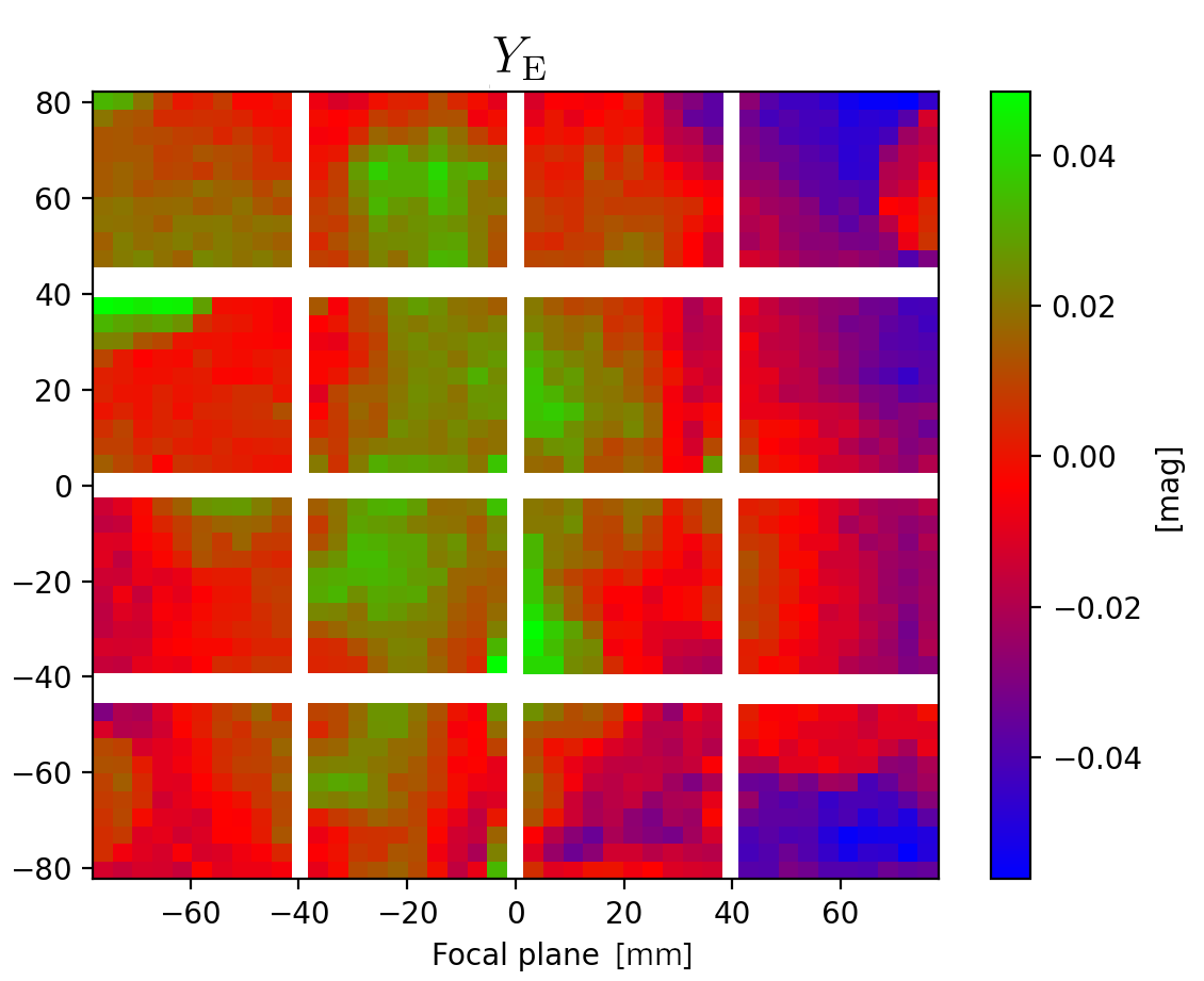
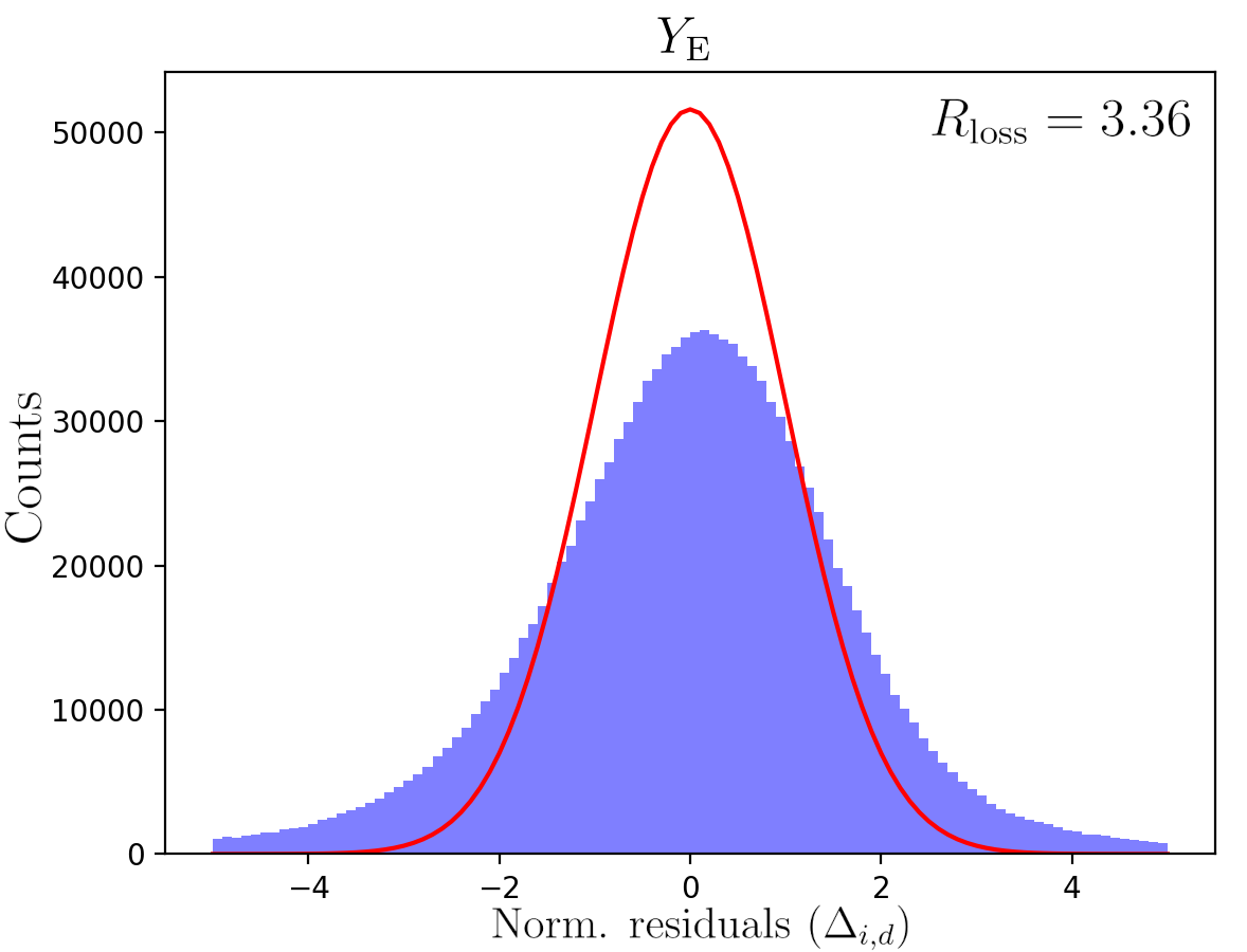
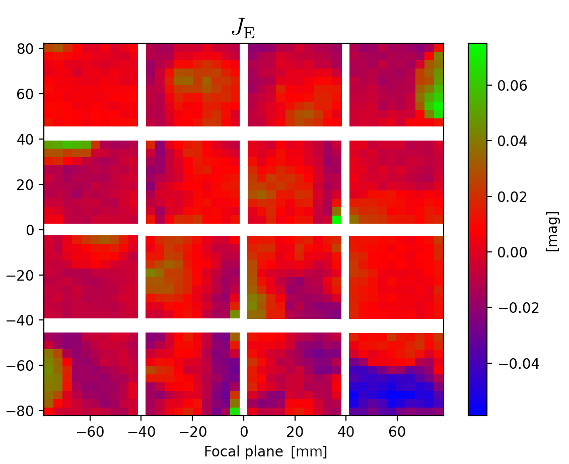
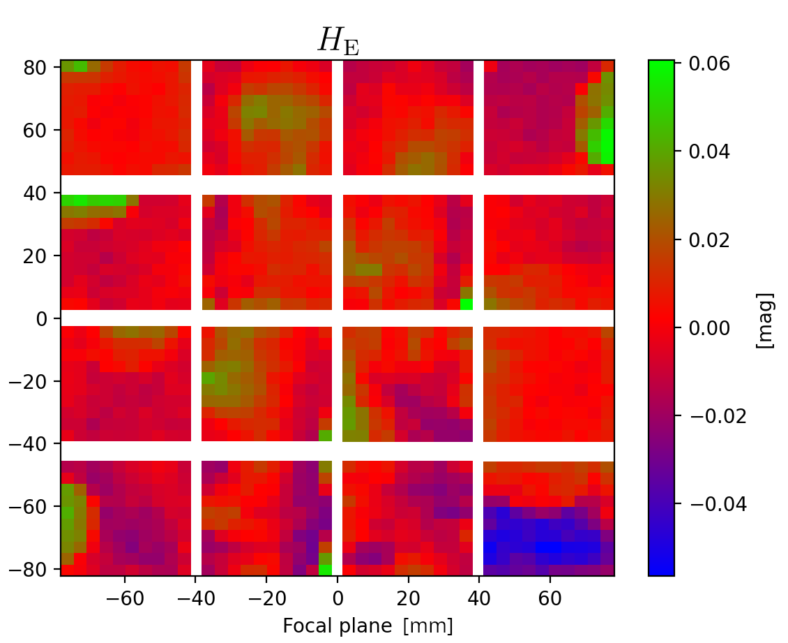
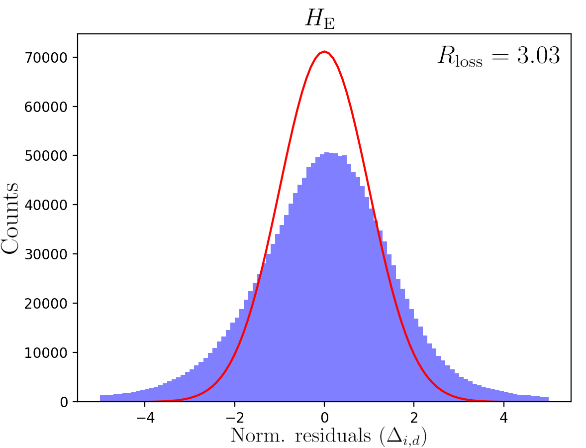
Figure 9: Left column: best-fit models of the $Y_{\scriptscriptstyle\rm E}$, $J_{\scriptscriptstyle\rm E}$, and $H_{\scriptscriptstyle\rm E}$ large-scale flats, ${\rm LSF}_{d}(x,y)$, as in Eq. 7. Right column: histograms of the normalised residuals of $\Delta_{i,d}(x,y)$ from Eq. 8, compared to a normal distribution with mean zero and variance one (red curve). The quantity $R_{\rm loss}$ from Eq. 9 is reported in the plots.

An alternative measure of the goodness-of-fit is given by the standard deviation of the observed magnitudes, once corrected for the large-scale flat and average sensitivity. That is, for the $i$-th source,

$$\sigma_{i}={\rm std}\left[m_{i,d}(x,y)-{\rm LSF}_{d}(x,y)-s_{d}\right]\,,$$ (10)

where the standard deviation is calculated over all $d$, $x$ and $y$ for which we have an observation of the $i$-th source. If the LSF and average sensitivity corrections are good enough, that is if $R_{\rm loss}\approx$ 1, we expect $\sigma_{i}$ to be approximately equal to the average of the magnitude uncertainties for the same $i$-th source, that is $\sigma_{i}\sim\langle\delta m_{i,d}(x,y)\rangle$. On the other hand, if the corrections are suboptimal and $R_{\rm loss}>1$, we expect $\sigma_{i}>\langle\delta m_{i,d}(x,y)\rangle$. Figure 10 shows the distributions of $\sigma_{i}$ versus the corresponding $m_{i}$ values for the three filters (in blue). We also show two more quantities. First, the distributions of the ‘uncorrected’ $\sigma_{i}$, namely the standard deviation of the $m_{i,d}(x,y)$ alone (in red), which are always larger than the ‘corrected’ $\sigma_{i}$, otherwise the use of the large-scale correction would be detrimental. And second, the distributions of the average magnitude uncertainties $\delta m_{i,d}(x,y)$ (in black), which are always smaller than the ‘corrected’ $\sigma_{i}$, since the large-scale flat algorithm cannot recover the random errors intrinsic to the flux measurements.

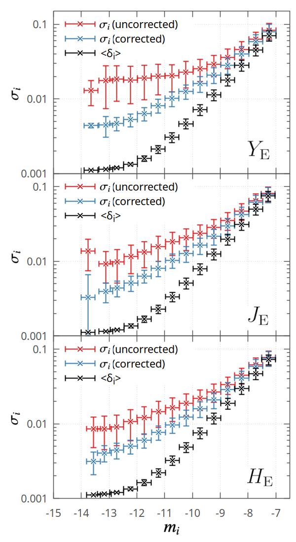
Figure 10: Comparison of the scatter in magnitude from the repeated observations of the same source (‘uncorrected’ $\sigma_{i}$, red symbols), with the same scatter after the large-scale flat ($\sigma_{i}$ from Eq. 10, blue symbols), as a function of the instrumental magnitude $m_{i}$ for the $Y_{\scriptscriptstyle\rm E}$, $J_{\scriptscriptstyle\rm E}$, and $H_{\scriptscriptstyle\rm E}$ filters. Also shown are the average of the photometric uncertainties for references (black symbols). The scatter introduced by the large-scale non-uniformities is represented by the separation between red and black symbols, while the blue symbols represent the residual scatter after the application of the large-scale flat calibration.

The separation between the blue and red symbols for the brightest sources provides a hint of the photometric offsets due to the ${\rm LSF}_{d}$ and $s_{d}$ contributions, which is of the order of 0.01 mag in all filters. These offsets are partially corrected by the application of the large-scale flat, by 0.006–0.007 mag for the brightest sources. At instrumental magnitudes $m_{i}\gtrsim-9$ the photometric uncertainties become comparable to the ‘uncorrected’ $\sigma_{i}$, that is, the large-scale-flat correction is negligible for the faintest sources.

We started this section by motivating the large-scale flat with the illumination properties of the telescope, and the LEDs’ Lambertian cosine profile, which are purely optical and geometrical effects. One would thus expect a fairly uniform pattern, whereas the derived large-scale flats shown in Fig. 9 look rather feature-rich. Some of the features, such as in the upper and lower right detectors, show almost discrete jumps between resolution elements ($200\times 200$ NISP pixels). This indicates variations on scales smaller than what the large-scale flat can resolve, consistent with underfitting suggested by $R_{\rm loss}\approx 3$. The inability of the model to fully resolve these variations is also evident when considering the histograms of the normalised residuals, $\Delta_{i,d}$. They are not Gaussian with a variance equal to one. Euclid’s optical design precludes such effects, hence the large-scale flat algorithm is picking up systematics in the photometry that are not fully corrected for by the preceding calibration efforts.

We argue that these features are due to low-level, diffuse charge persistence (Sect. 3.1.5) that is not captured by our masking efforts. Plausibly, this is caused by the alternating higher and lower zodiacal background registered by the detectors as we cycle through different filters and grisms in the ROS. Indeed, these features have a remarkable resemblance to those seen in our persistence-calibration data. This in itself is a remarkable confirmation that our large-scale flat implementation is working very well, because at no point is the algorithm informed about charge-persistence effects. Hence the large-scale flat correction does exactly what it is supposed to do: it sweeps up all residual effects that are left uncorrected – or imperfectly corrected – by the preceding calibration steps, regardless of their multiplicative, additive, or more complicated nature.

Figure 10 shows that the large-scale flat corrects about 6–7 mmag of the joint systematics in the photometry. It also shows that we still lack the remaining 2–3 mmag to bring the blue symbols closer to the black ones, also for the brightest magnitudes. We conclude that the relative photometric accuracy of the Q1 data after the large-scale flat correction has a floor of at least 2–3 mmag. A persistence correction – as opposed to masking in Q1 – in a future data release should considerably improve the photometry further.

3.2.3 Background estimation

We capture background variations while simultaneously minimising the influence of bright objects on the background estimates. The background maps are estimated in several steps using SourceExtractor (Bertin & Arnouts 1996). First, a local background is calculated in a rectangular area by iteratively clipping the histogram of the pixel values until the value converges at 3 $\sigma$ around the median. The background value is set to the mode of the histogram defined by

$$\rm{mode}=2.5\,{\rm median}-1.5\,{\rm mean}\,.$$ (11)

The size of the rectangular area in the background-subtraction task is set to $64\,\times\,64$ pixels. The background grid computed this way is subsequently median filtered using a $3\,\times\,3$ box to eliminate high background estimates due to bright stars. The final background image is given by a spline interpolation over the grid values. This is not subtracted from the corresponding scientific image, and it is provided as a companion file (Sect. 4).

While this method provides consistent results for the compact and faint objects at the core of the Euclid science programme, it results in considerable over-subtraction for extended, bright galaxies, limiting for example studies of low-surface brightness features and other faint, diffuse targets. A more refined method will be implemented for DR1.

3.2.4 PSF modelling from physical optics

The ‘MDB mode’ of the NIR_PointSpreadFunction module can derive PSF images for single exposures only. The PSF images are based on a library of PSF models that were derived from a physical-optics model of the telescope and instrument stored in the MDB. The PSF models account for different FPA positions and wavelengths, while also incorporating pixelisation and broadening effects, such as intra-pixel sensitivity and IPC (Le Graët et al. 2022).

The MDB mode cannot produce a PSF model for stacked images. This is because it is agnostic to: (i) the accuracy of the astrometric solver (Sect. 3.2.7) that corrects for dither offsets and optical distortions; and (ii) the resampling methods and performance of the stacking software (out-of-scope for this paper).

3.2.5 PSF modelling from data

Contrary to the MDB mode, the ‘Inflight mode’ of the NIR_PointSpreadFunction module derives the PSF model directly from the data. This is the standard mode used for survey-data processing. It can derive a PSF model from single images, a series of dithered single images, and also from stacked images. The derivation of PSF models for stacked images is out of the scope for this paper, because NIR PF stacks are not included in Q1. Stacks are created by the MER processing function (MER PF) that is described in a separate Q1 paper (Euclid Collaboration: Romelli et al. 2025).

The Inflight mode utilises SourceExtractor and PSFEx (Bertin 2011) to detect and extract the sources in the images, and then to derive the PSF models from these data. A relevant parameter given to SourceExtractor is VIGNET that defines the size of the image stamp centred on each detected source. PSFEx uses these stamps to derive the PSF models. The larger the size of the stamps, the more extended the derived PSF model can be.

When run in the single-image mode, SourceExtractor produces a multi-extension FITS (MEF) catalogue with one extension per detector. When several images are provided, such as all dithers from the ROS in one photometric filter, a single extension in the MEF catalogue contains the sources from all dithers for that detector. In this way, the source density is increased proportionally to the number of exposures to improve the PSF model. The PSF comprises three components: (i) the optical PSF from the telescope and the instrument’s fore-optics; (ii) a detector-electronic PSF that describes charge-sharing processes between pixels during charge-generation and readout; and (iii) a mechanical PSF from the spacecraft’s tracking performance. While optical and detector PSFs are unchanged between dithers, the mechanical PSF may vary. The precondition for using the all-dither mode is therefore that the spacecraft’s tracking is uniform across dithered exposures.

This paper focuses on the all-dithers PSF models, which is also the default mode in NIR PF. Once the catalogues are created, they are passed to PSFEx that preselects suitable sources for PSF modelling. Only unflagged point sources can enter, that is CRs, saturated stars, and other compromised sources are excluded (see Sect. 3.1). PSFex then: (i) defines the size and sampling of the derived models; (ii) accounts for variability of the PSF shape across the FPA; and (iii) sets the level of details of the models. In particular, the PSF variability can be accounted for at the level of individual detectors, or for the FPA as a whole. Currently, the PSF shape is considered variable among detectors for all three NIR passbands. In addition, for the $Y_{\scriptscriptstyle\rm E}$ band, we include variations inside the detectors, which result in a better PSF reconstruction.

The detail in the PSF model depends on how accurately it reconstructs the shape of an observed unsaturated point source. PSFex models the PSF either directly from the image pixels, or as a linear combination of basis vectors. For this paper, we chose Gauss–Laguerre basis vectors (also known as polar shapelets; Massey & Refregier 2005) that have two free parameters configurable for PSFEx: BASIS_SCALE affects the width of the PSF profile; and BASIS_NUMBER defines the level of detail in the reconstructed core and wings. We tuned a set of optimal values by minimising the difference between PSF models from the Inflight and the MDB modes. The respective best values for BASIS_SCALE and BASIS_NUMBER currently used by NIR PF are 1.4 and 5 for $Y_{\scriptscriptstyle\rm E}$ band, 1.38 and 9 for $J_{\scriptscriptstyle\rm E}$ band, and 1.7 and 5 for $H_{\scriptscriptstyle\rm E}$ band.

Figure 11 shows the 2D PSF models at the centre of each detector and for all passbands, using data from four dithered exposures of the EWS (ObservationId 3800). The number of sources effectively used by PSFEx ranges from 30 to 40 for each dither, depending on the detector. The sampling is $0.\mathrm{″}05$, the same as the MDB models and corresponding to 1/6th of the NISP pixel size. The PSFs models recover the known trefoil shape (Euclid Collaboration: Mellier et al. 2024) of Euclid’s optics, and show that the PSF is very stable across the field of view.

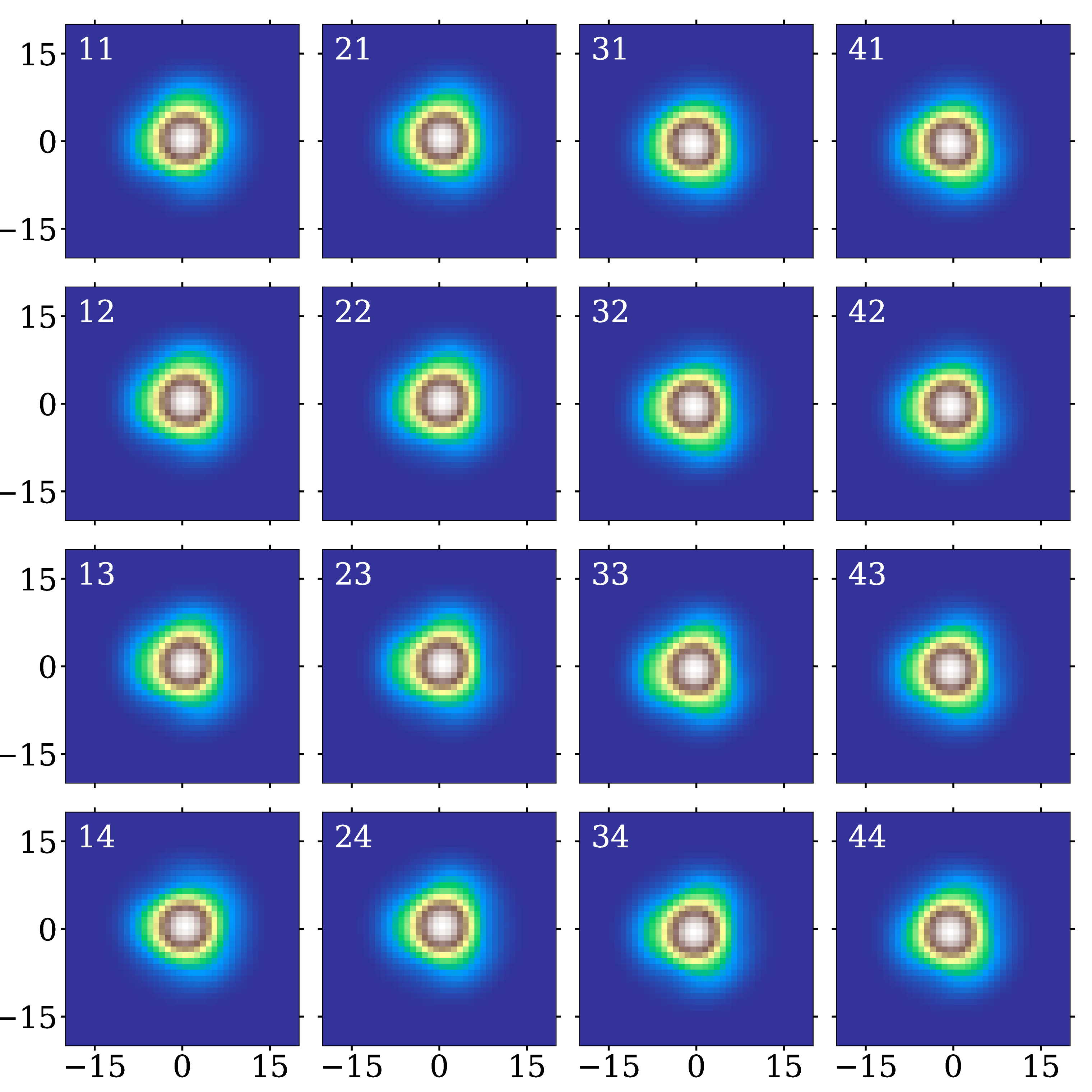
Figure 11: 2D NISP PSF models derived from a typical EWS observation. The different panels are for $Y_{\scriptscriptstyle\rm E}$ (left), $J_{\scriptscriptstyle\rm E}$ (middle), and $H_{\scriptscriptstyle\rm E}$ (right) passbands and show the models (40$\times$40 pixel stamps) derived for each of the 16 NISP detectors. The resolution here is $0.\mathrm{″}05$, subsampling the NISP pixel scale by a factor of 6.

Figure 12 shows the encircled-energy curves for all detectors in each passband. The radii encircling 50% (rEE50) and 80% (rEE80) of energy must fulfill two mission requirements on the compactness of the PSF. Specifically, ${\rm rEE50}<$$$ and ${\rm rEE80}<$$$ for all wavelengths below 1486 nm, meaning all of the $Y_{\scriptscriptstyle\rm E}$ band and most of $J_{\scriptscriptstyle\rm E}$ band. The figure shows that even the reddest passband, $H_{\scriptscriptstyle\rm E}$, easily meets these requirements, a testament to the excellent NISP optics (see also Grupp et al. 2019).

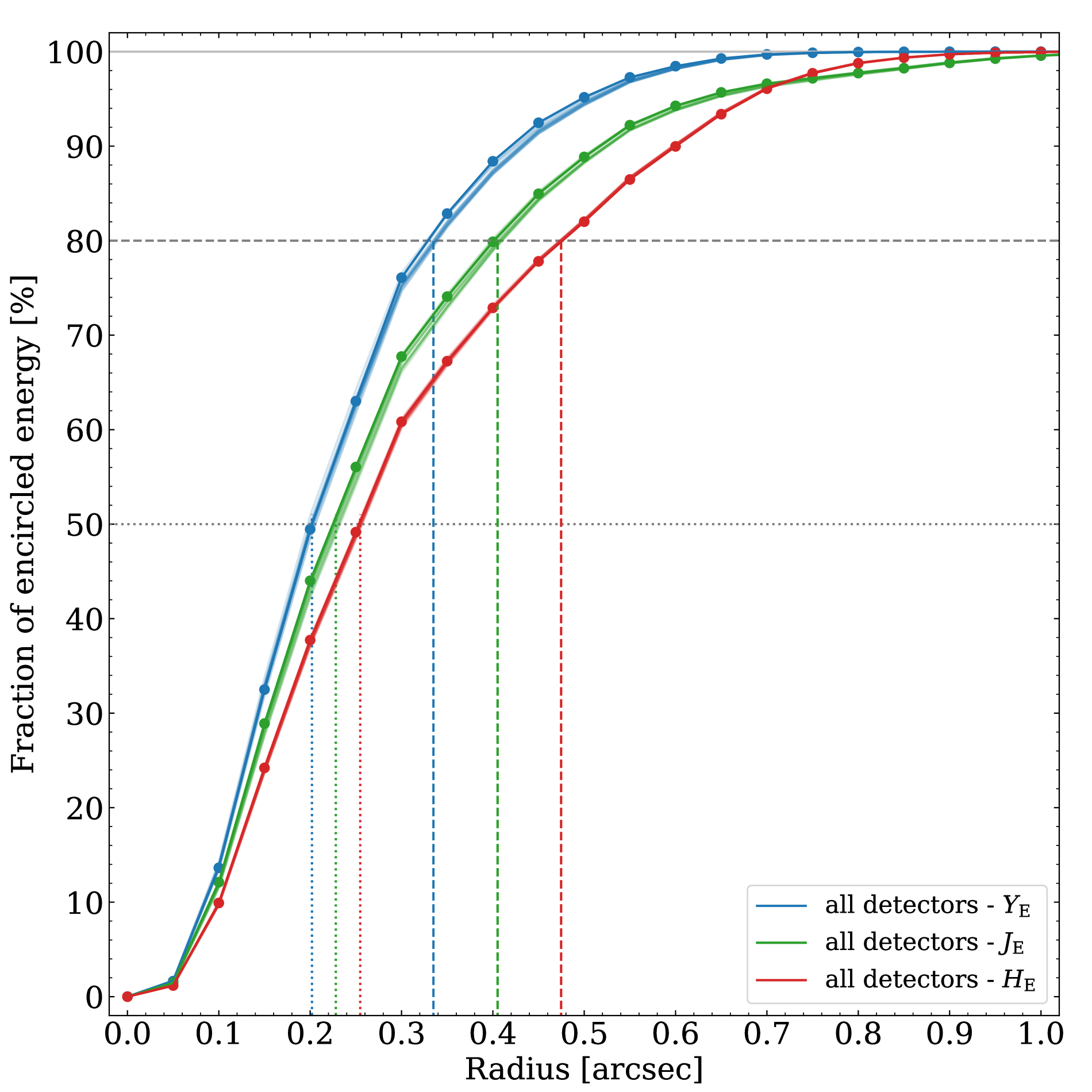
Figure 12: Fraction of encircled energy as a function of the distance to the peak of the PSF profile. These curves were calculated using the same models shown in Fig. 11 for each of the 16 detectors of the three NISP passbands. The vertical and horizontal lines indicate the average radii encircling 50% (rEE50, dotted lines) and 80% (rEE80, dashed lines).

3.2.6 Quality of the PSF model from PSF-fitting photometry

The quality of the PSF models can be further investigated by PSF-fitting photometry. To this end we pass the PSF model to SourceExtractor, which in turn fits the models to every source extracted from the images. Figure 13 (right panels) compares the PSF magnitudes (MAG_PSF) to aperture magnitudes (MAG_APER) with a diameter of 6 pixels, the default in NIR PF. This aperture then contains – for the current models – about $99.99$% for $Y_{\scriptscriptstyle\rm E}$, $98.8$% for $J_{\scriptscriptstyle\rm E}$, and $99.7$% for $H_{\scriptscriptstyle\rm E}$ of the total flux. Aperture corrections compensate for these offsets during absolute photometric calibration (Sect. 3.2.8). The three panels in Fig. 13 are colour-coded according to the FLUX_RADIUS, which contains a certain fraction of a source’s total flux. To obtain the half-light radius encompassing half of the total flux, one would set ${\rm{\tt PHOT\_FLUXFRAC}}=0.5$. Figure 13 (left panels) shows the distribution of the half-light diameter, or two times the FLUX_RADIUS, including both point- and extended sources. For each passband, we highlight the range in which the point sources are located. These are the FLUX_RADIUS ranges of the sources passed to PSFex to derive the PSF models (the same sources plotted in the right panels).

The right column in Fig. 13 shows that the PSF-fitting photometry for $H_{\scriptscriptstyle\rm E}$ band agrees to better than 1% with the aperture photometry. For the $J_{\scriptscriptstyle\rm E}$ band we see that PSF magnitudes are systematically brighter by about 3%. For the $Y_{\scriptscriptstyle\rm E}$ band, the offset increases to more than 6%, there is a slight dependence on magnitude, and the scatter is considerably larger than for the other two bands. For all three bands we also find a positive correlation between FLUX_RADIUS on the one hand, and the offset and the scatter on the other hand. For the $H_{\scriptscriptstyle\rm E}$ band, in particular, the slope of the linear regression is more prominent for more extended sources. There is ongoing work to improve the PSF models. In section 5.1 of Euclid Collaboration: Jahnke et al. (2024), we show preliminary results of PSF models derived using a larger number of point sources from self-calibration observations instead of an EWS field, a larger number of basis vectors (hundreds instead of tens), and in $$$\times$$$ stamps instead of $$$\times$$$ for each source. These updates require changes in the PSFex configuration that will be implemented for the next data release.

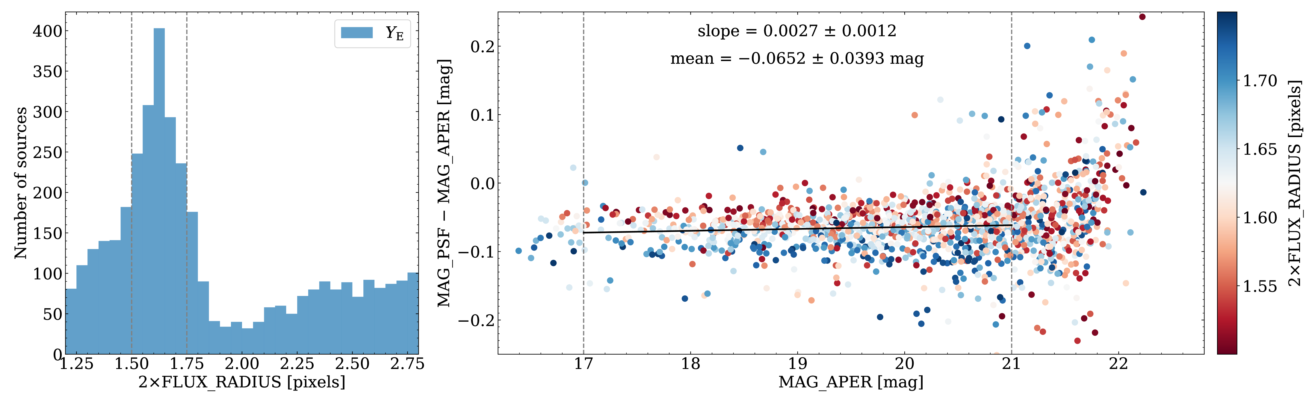
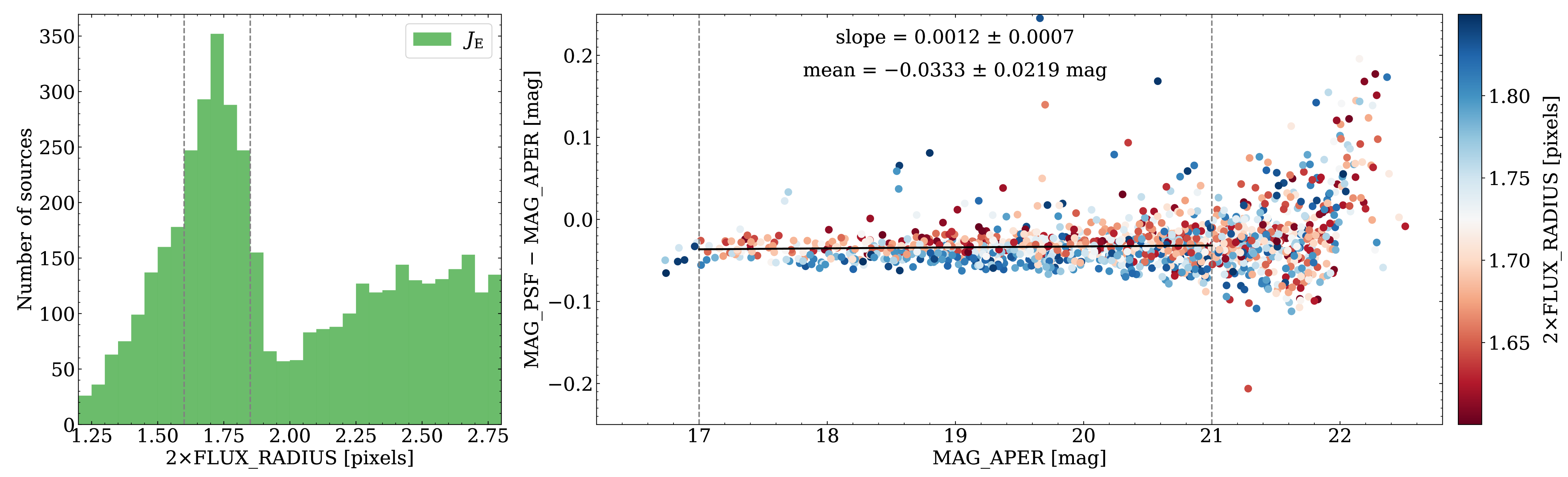
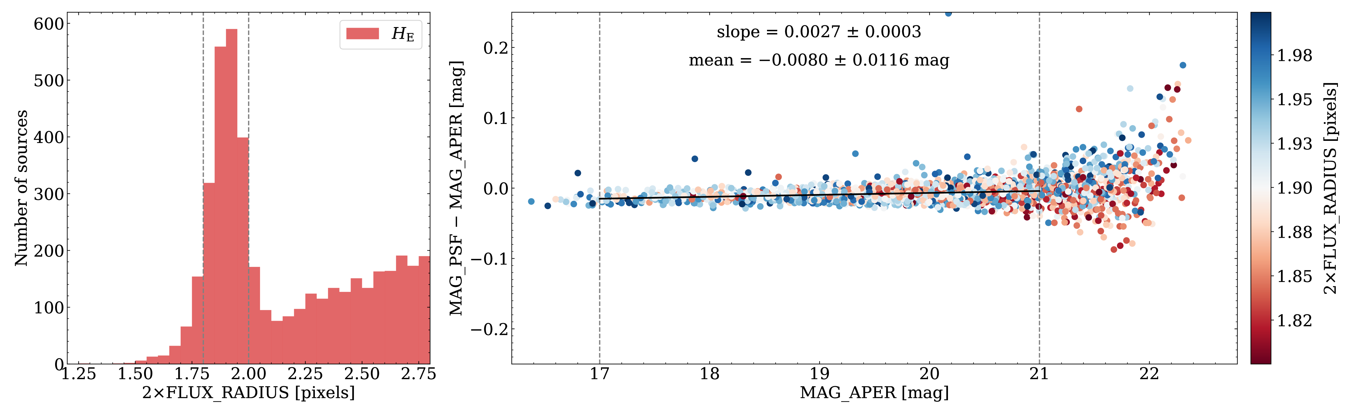
Figure 13: Comparison between PSF-fitting and aperture photometry. Left column: Histograms of the half-light diameter for the three NISP passbands. The dashed lines indicate the ranges of point-sources plotted in the right panels and used by PSFex for PSF modelling. Right column: Difference between MAG_PSF and MAG_APER, colour-coded according to the half-light diameter. The mean difference and the slope of the linear regression (black line) for magnitudes between 17 and 21 (dashed lines) are also shown.

3.2.7 Astrometric calibration

Astrometric calibration accounts for geometric distortions from instrument optics and focal-plane metrology, which define detector positions and orientations. For each pointing and band, this is done by minimising positional differences between sources detected in dithered exposures and those in an external reference catalogue. Currently, Gaia DR3 (Gaia Collaboration et al. 2023) is preferred over the VIS catalogue (Euclid Collaboration: McCracken et al. 2025), since its bright stars – saturated in VIS – remain unsaturated in NISP, providing more reliable reference sources.

Astrometric calibration is performed using SCAMP (Bertin 2006), which operates on catalogues rather than images. This requires both a reference catalogue and source catalogues for the dithered exposures. Source catalogues are provided by SourceExtractor with a configuration optimised for astrometric calibration. The astrometric solution – modelled in NIR PF as a 3rd-order polynomial per detector – is derived by minimising the $\chi^{2}$-sum of positional differences between overlapping detections.

In some cases, particularly when too few stars are available in common with the external catalogue for certain detectors, SCAMP may fail to converge unless its parameters are fine tuned. However, the optimal parameters can vary across fields with different stellar densities. To address this, we implemented an astrometric pre-solution, that is an initial model for geometric distortion along with the relative positions and orientations of the detectors. This pre-solution helps reduce sensitivity to the initial matching radius with the external catalogue. If the radius is too large, it can cause false matches. If it is too small, it may result in no matches, especially near the field edges, where distortion can shift source positions by up to $10\mathrm{″}$. As a result, the robustness of the distortion-model fitting is significantly improved.

The astrometric pre-solution is created by the distortion-model pipeline in NIR PF, where SCAMP is run on the 76 dithered exposures, per band, of the self-calibration field. SCAMP, following the polynomial PV convention (Calabretta & Greisen 2002), applies the distortion polynomial to the world coordinates. Therefore, when transferring the pre-solution to a different dither, adjusting for the different dither’s rotation on the sky is required. This is is done by first converting the pre-solution to the Simple Imaging Polynomial (SIP) convention (Shupe et al. 2005), where the distortion is instead applied to pixel coordinates. It is then translated back to the PV convention using the dither’s centre and rotation, as encoded in the world coordinate system (WCS) keywords. Currently, these transformations use polynomial fitting functions. An analytic conversion method (see e.g., Shupe et al. 2012) will be used for the next data releases.

3.2.8 Photometric calibration

For Euclid’s cosmology science aims, we have an accuracy goal of 5% on the absolute flux calibration of NISP. This comes easily, since we calibrate against spectrophotometric white dwarfs in HST CALSPEC, which have an estimated accuracy of 1% (Bohlin et al. 2014, 2017, 2020).

For NISP imaging we could use the all-sky faint WDs network (Narayan et al. 2019; Bohlin et al. 2024) in CALSPEC. However, none of them are visible in Euclid’s continuous viewing zones that extend $2.\mathrm{°}5$ from the ecliptic poles. We therefore established a faint WD, WDJ175318.65+644502.15 (Gaia SourceID 1440758225532172032) in the self-calibration field near the NEP. This was tied to CALSPEC using photometric and spectroscopic HST observations with WFC3/IR and STIS (programme IDs 16702 and 17442, Appleton et al. 2021; Deustua et al. 2023). This star is stable to within $1\%$ over timescales ranging from 100 seconds to several years. With $H_{\scriptscriptstyle\rm E}=18.36$, it is faint enough for NISP, which saturates at around 16.5 AB mag.

Flux calibration is established by comparing the observed flux $F_{\mathrm{obs}}$ in instrumental units (e^- s^-1) with the true flux $F_{\mathrm{true}}$ in $\mathrm{\muup}$Jy. The true flux integrated over a passband is obtained by convolving the WD’s model spectral flux density $S_{\nu}$ with the passbands’ spectral response $T(\nu)$,

$$F_{\mathrm{true}}=\frac{\int\dfrac{T(\nu)\,S_{\nu}}{\nu}\,{\rm d}\nu}{\int\dfrac{T(\nu)}{\nu}\,{\rm d}\nu}\,.$$ (12)

Here, $\nu$ is the frequency, and the spectral response $T(\nu)$ for passbands $Y_{\scriptscriptstyle\rm E}$, $J_{\scriptscriptstyle\rm E}$, and $H_{\scriptscriptstyle\rm E}$ is taken from Euclid Collaboration: Schirmer et al. (2022).

$F_{\mathrm{obs}}$ is measured with SourceExtractor within a fixed aperture of diameter 6 pixels. We use our PSF model (Sect. 3.2.5) to compute the fraction of the flux that falls outside this aperture, and correct $F_{\mathrm{obs}}$ accordingly. Finally, the absolute flux calibration factor, or inverse sensitivity (IS) in NIR PF, is defined as

$$\mathrm{IS}=\frac{F_{\mathrm{true}}\,[\mathrm{\muup Jy}]}{F_{\mathrm{obs}}\,[\mathrm{e}^{-}\,\mathrm{s}^{-1}]}\,.$$ (13)

Flux calibration of the Q1 data is based on the self-calibration observations – that contain the WD – in June 2024 (see Sect. 5.2). Figure 14 presents the individual measurements of the WD in two NISP detectors, together with the corresponding IS. As can be seen, the 3 $\sigma$ uncertainty of the IS is well within the required $5\%$ boundary.

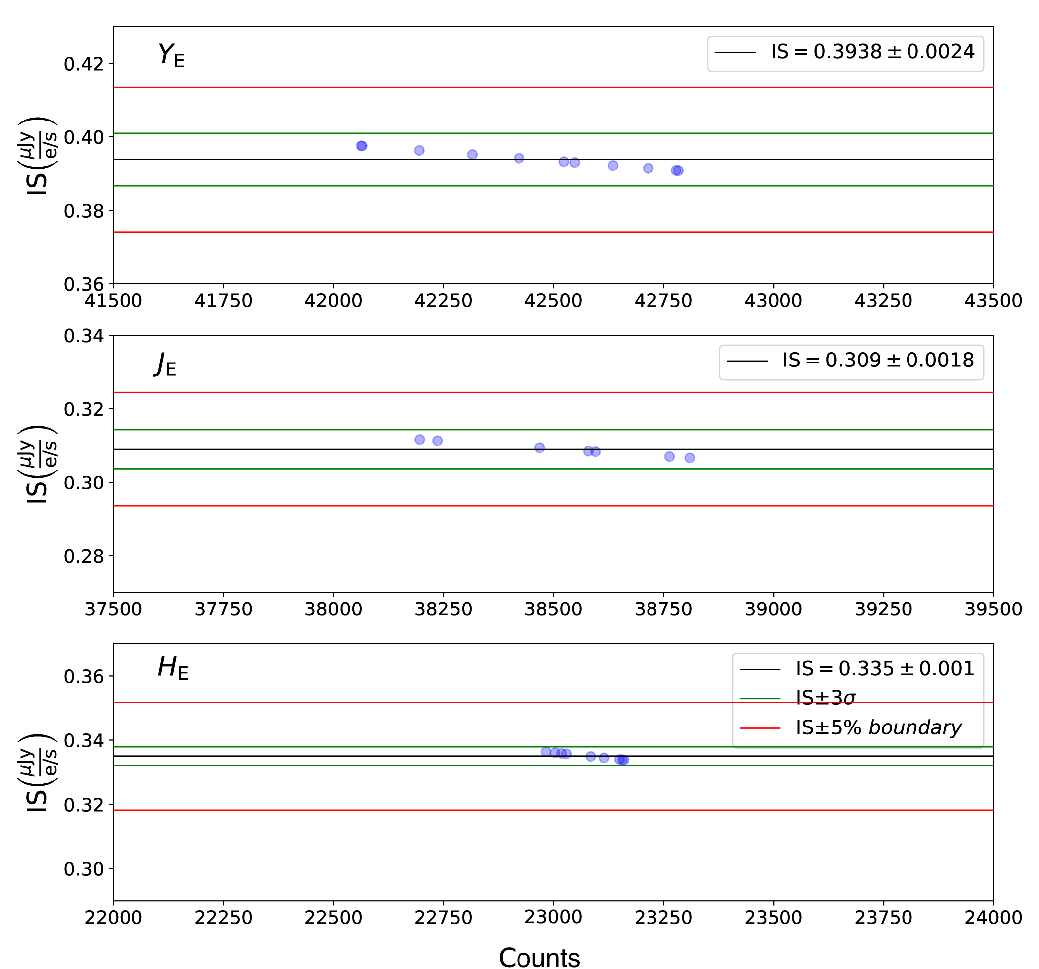
Figure 14: Absolute flux calibration factor IS as a function of the observed counts, from the June 2024 WD calibration observations used for Q1. The observed counts were corrected for aperture losses. The black and green lines indicate the respective sigma-clipped mean of the individual IS measurements and the sample’s 3 $\sigma$ uncertainty. The red lines denote the 5% requirement.

3.2.9 Ghost masking

Although a number of ghosts are seen within the NISP-P data (see Euclid Collaboration: Jahnke et al. 2024), only the dichroic and filter ghosts are masked in Q1. The ghosts’ size, shape, and position relative to their bright source stars are described in detail in Paterson et al. (in prep.). There, we also discuss the dependence on the filter used, detection methods, and lower flux limits that require masking. For the masking itself, we first select all stars from Gaia brighter than the magnitude limit set by Paterson et al. (in prep.). Pixels that fall within the computed masking area of these stars are then flagged with GHOST (bit 18) and INVALID (bit 0) in the DQ layer Appendix B.

Stars brighter than 11 mag also exhibit an arc with a curvature radius of about $1.\mathrm{\prime }7$ (see figure 19 of Euclid Collaboration: Jahnke et al. 2024). The arcs extend up to $\pm\,45$\mathrm{\SIUnitSymbolDegree}$$ from the $x$-axis in pixel coordinates. These ghosts are the result of charge persistence that accumulates when NISP switches between filters and grisms (Euclid Collaboration: Jahnke et al. 2024). The procedure to mask these arcs is similar to that of the ghosts. First, bright stars expected to produce arcs are selected from Gaia. Second, affected pixels are flagged with both PERSIST (bit 13) and INVALID in the DQ layer.

3.2.10 Catalogue production

The final step of NIR PF is catalogue extraction, producing primarily single-band catalogues for the calibrated individual and stacked images. Stacked images and their catalogues, however, are beyond the scope of this Q1 paper and we refer to MER PF instead (Euclid Collaboration: Romelli et al. 2025). In the following, we describe NIR_CatalogExtraction that operates on individual calibrated images, processing one dither at a time on a detector-by-detector basis. The module consists of two main steps, the first generates the source map, which is subsequently passed to the second step as a detection constraint for extracting source photometry.

The identification process begins by computing the second derivative of the image along four distinct directions. This technique is based on the CuTEx tool (Molinari et al. 2011). Since two-dimensional images represent discrete data sets, we employ Lagrangian methods for numerical differentiation, specifically using the 3-point formula (detailed in Hildebrand 1956). For each pixel in the input image, the algorithm applies a convolution with a kernel derived from the second-order derivative formulas along four directions ($x$, $y$, and the two $45$\mathrm{\SIUnitSymbolDegree}$$ bisectors). This ensures that the results are independent of the derivation direction. The resulting second derivative map is then used to detect objects and construct the source map, a technique that proves highly effective in crowded regions as well as in the presence of variable background without the need for dedicated tunings.

A dynamic threshold is applied for source identification, with its value automatically adjusted by the code through iterative refinement. Starting from an initial threshold, the algorithm calculates the number of detected sources and evaluates how many of these allow reliable PSF photometry. The threshold is iteratively optimised to balance source detection with photometric reliability. Once the optimal threshold is determined, a mask is generated to mark the source positions. This mask is subsequently used as input for the photometry step, where SourceExtractor processes the calibrated dither, constrained by the detection map for source positions.

The version of the code used for Q1 simultaneously performs three types of photometry for each detected object: aperture with a fixed radius of 3 pixels; automatic; and PSF fitting. Consequently, the module requires the PSF model computed by NIR_PointSpreadFunction as additional input. As discussed in Sect. 3.2.5, the fixed aperture adopted for catalogue extraction includes most of the flux for compact objects: 99.99% for $Y_{\scriptscriptstyle\rm E}$; 98.8% for $J_{\scriptscriptstyle\rm E}$; and 99.7% for $H_{\scriptscriptstyle\rm E}$.

The final output catalogue is stored as a FITS file containing 16 layers, one for each detector, to maintain correspondence with the structure of the calibrated image (Sect. 3.2.10). This approach ensures efficient and accurate extraction of sources and their photometric properties.

3.3 DQC pipeline

The LE 1 data from the selected sky patches in this release are processed using NIR PF, generating a set of Data Products per pipeline run (see Sect. 4). These DPs must be verified to ensure data quality meets the required standards.

The data quality control (DQC) pipeline inspects NIR PF DPs by checking the DQC parameters computed during processing. These parameters are stored as metadata and ingested into the Euclid Archive System (EAS) at the end of each run.

Each DQC pipeline run produces a PDF report for each input pipeline processing order (PPO) ID. The report contains test results, with each test consisting of multiple checks. In each check, selected DQC parameters from a given DP are compared against predefined thresholds to determine compliance. Test results fall into four categories: PASS, FAIL, WARN, or N/A. We maintain the list of parameter thresholds for verification.

Each test result is recorded at the beginning of the PDF report and stored in a local database. We review a summary table of all test results for a sky patch before approving them for publication. The available tests include specific and shared tests for both NIR PF and SIR PF, which check technical aspects such as input/output products and profiling. For this release, the tests use calibrated images and catalogues to evaluate PSF quality, flagged pixel percentage, astrometric RMS, background level, and photometric accuracy.

4 NIR Data Products

The Euclid Common Data Model is an XML schema (XSD) that defines all Euclid Data Products, along with a dictionary of all data types, interfaces, and FITS file formats. A Data Product is therefore represented as an XML file containing the names of data files and their corresponding metadata, which can be stored in and retrieved from the EAS.

A detailed description of the metadata for all NIR DPs is available in the Data Product Description Document (DPDD, Euclid Collaboration 2025). The DPs produced by NIR PF for Q1 are the DpdNirCalibratedFrame and the corresponding DpdNirCalibratedFrameCatalog.

4.1 Calibrated exposures

The DpdNirCalibratedFrame is a fully astrometrically and photometrically calibrated exposure, obtained by applying calibration products and corrections to each individual LE1 photometric image. Image data are stored as FITS files referenced in the DP and are organised into three main sections: DataStorage; BackgroundStorage; and PsfStorage.

DataStorage references the main MEF file that contains the calibrated image data. This file consists of a total of 49 header data units. The first HDU or primary header stores the main metadata keywords of the observation sequence that acquired the exposure. For each detector, three HDUs are provided: (i) SCI, containing the scientific image data in electrons; (ii) RMS with the associated root mean square; and (iii) DQ with the data-quality mask for each pixel (Appendix B). The header of each SCI HDU contains the detector WCS and the zero point.

BackgroundStorage references the FITS file of the background image, computed during the background-estimation step (Sect. 3.2.3). Its file structure mirrors that of the scientific image described above.

The PsfStorage section of the DP refers to two FITS files: the PSF model; and the corresponding PSF image (Sect. 3.2.5).

Another key metadata tag is QualityParams, which contains a structure to store image-quality parameters and statistics. They are used as input for the DQC pipeline (Sect. 3.3) and are computed by specific tasks in NIR PF.

4.2 Calibrated catalogues

The DpdNirCalibratedFrameCatalog is the source catalogue extracted from the calibrated exposure, as described in Sect. 3.2.10. Its global metadata structure mirrors that of DpdNirCalibratedFrame. The MEF catalogue produced is referenced under the DataStorage tag of the DP and is structured into 17 HDUs: a primary header followed by a data HDU for each detector.

The data HDUs store the source catalogue tables, which include coordinates, size, ellipticity, fluxes, and magnitudes extracted using three different methods by SourceExtractor: APER, AUTO, and PSF, as described in Sect. 3.2.10.

5 Results for Euclid Quick Release 1

Q1 includes one visit for each of the three Euclid Deep fields, North, South and Fornax, as well as observations of the Lynd’s Dark Nebula LDN1641, covering a total of 63.1 ${\rm deg}^{2}$ (Euclid Collaboration: Aussel et al. 2025). From an initial set of 1620 NISP raw exposures, we rejected seven images that did not pass the DQC pipeline (0.4%), while the remaining 1613 images are available from the Euclid Science Archive.

In the following sections we provide a characterisation of the astrometric and photometric accuracy of the NIR Q1 data set.

5.1 Accuracy of astrometric and photometric calibration based on Gaia DR3

As discussed in Sect. 3.2.7, the astrometric calibration is referenced against Gaia DR3 (Gaia Collaboration et al. 2023) and accounts for proper motion. Astrometric residuals are about 15, 12, and 9 mas, respectively, for the Euclid $Y_{\scriptscriptstyle\rm E}$, $J_{\scriptscriptstyle\rm E}$, and $H_{\scriptscriptstyle\rm E}$ bands as shown in Fig. 15. The residuals are well within the required accuracy of 100 mas.

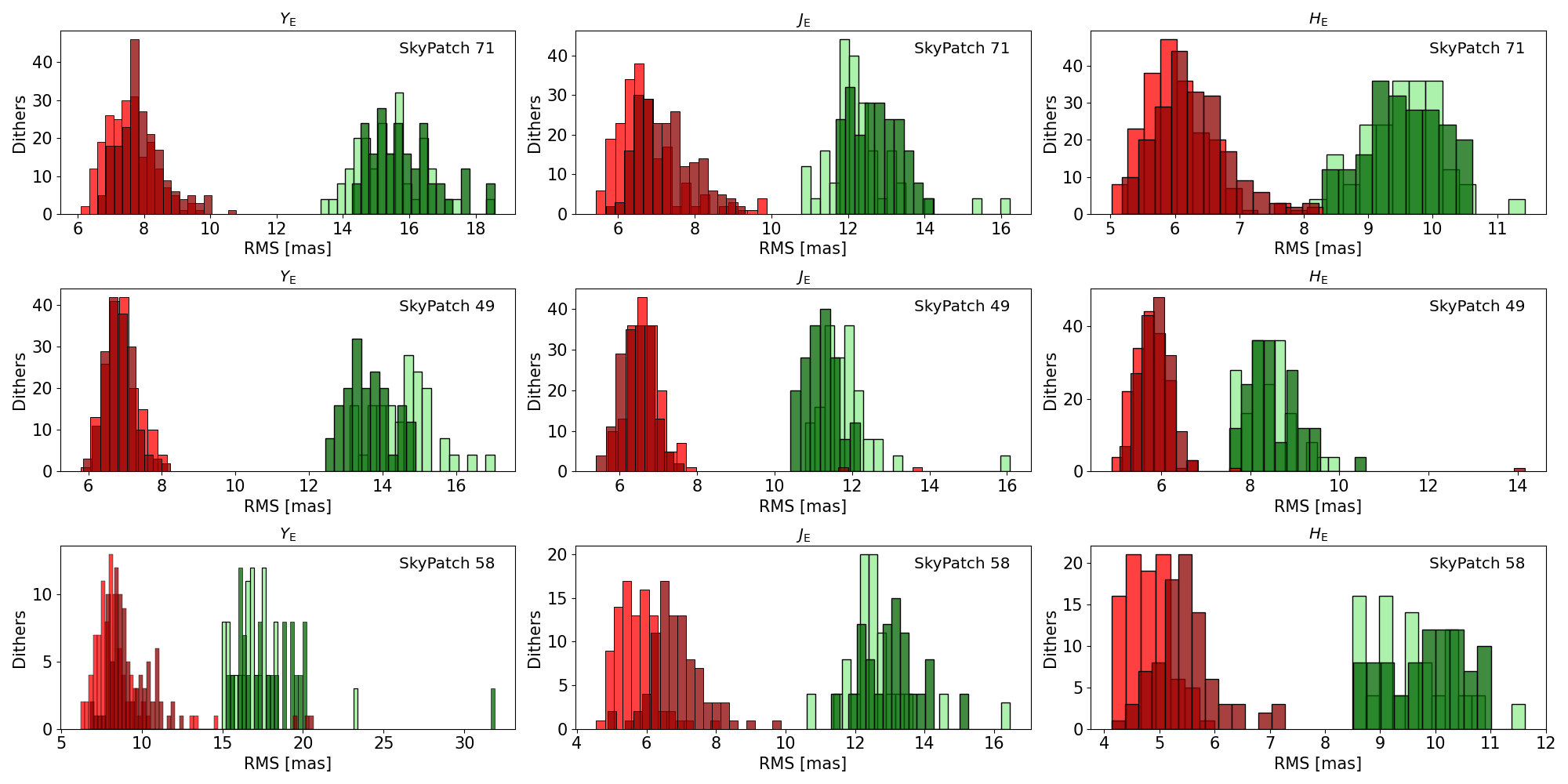
Figure 15: Astrometric RMS residuals for dithers in the three Q1 sky patches. The red histograms are the residuals obtained from overlapping detections (required accuracy: 100 mas), while the green histograms illustrate residuals obtained through comparison with Gaia positions (required accuracy: 200 mas). The RMS for $\Delta\alpha\cos(\delta)$ and $\Delta\delta$ are represented by light and dark shading, respectively. The residuals are always well within the required accuracies.

We also evaluated possible systematic effects related to the source position in the focal plane. For a given Q1 sky patch, the NIR PF source catalogues were cross-matched against Gaia DR3. Then we binned the angular distances between Euclid and Gaia positions as a function of focal-plane coordinates, taking the median value for each bin. Figure 16 shows that the astrometric accuracy has no major spatial dependence apart from a slight increase for one detector in the $Y_{\scriptscriptstyle\rm E}$ band, still well below 1/10th of a pixel. The other Q1 sky patches behave similarly.

Figure 16: Focal plane distribution of position error with respect to Gaia, combining all sources for sky patch 71.

In much the same way we analyse the positional dependence of the photometric zero points. After cross-matching with Gaia DR3, we consider the difference between Euclid and Gaia magnitudes after correcting Gaia $G_{\mathrm{RP}}$ for a colour term,

$$G_{\mathrm{RP}}^{\mathrm{Corr}}=G_{\mathrm{RP}}+A+B\,(G_{\mathrm{BP}}-G_{\mathrm{RP}})\;,$$ (14)

where $A$ and $B$ are computed for each Euclid filter. Results for sky patch 71 are reported in Fig. 17, showing that the photometric accuracy has no major spatial dependence. The only visible effect is an increase by about 0.02 mag for detector DET13 in the $Y_{\scriptscriptstyle\rm E}$ band. We note that the photometric residuals for the same detector for sky patch 49 are much smaller, suggesting a slow drift in the photometric calibration for this detector in $Y_{\scriptscriptstyle\rm E}$ band. Indeed, each detector shows a slightly different evolution of the photometric zero point over time. In this respect, DET13 has the strongest evolution, which is not perfectly modelled by the relative calibration in the Q1 data set. Further refinements will be developed and applied for DR1 and later data releases.

Figure 17: FPA distribution of photometric residuals for sky patch 71 between $Y_{\scriptscriptstyle\rm E}$, $J_{\scriptscriptstyle\rm E}$, $H_{\scriptscriptstyle\rm E}$, and Gaia photometry, after correcting for the colour term.

5.2 Zero-point stability from self-calibration observations

A complementary way to assess calibration accuracy and photometric stability – specifically, variations in filter throughput and zero points – is to analyse the monthly self-calibration observations. This field is visited with a 76-point dither pattern, providing – among many other purposes (Euclid Collaboration: Mellier et al. 2024) – a baseline for monitoring Euclid s spectrophotometric response.

The key advantage of this approach is the ability to compare fluxes across thousands of sources distributed over different detectors, within and between visits. This minimises uncertainties compared to absolute calibration based on the single WD spectrophotometric standard.

For this comparison, we used two self-calibration visits in July and August 2024 that were close in time to the Q1 observations. We take the July visit as a reference and compute magnitude differences with respect to the August visit. Both data sets were processed with the same calibration products, so that any differences would originate from actual throughput variations.

Specifically, we took the stacked-frame catalogue from July and cross-matched it with the 76 catalogues from the individual exposures of that month, using a matching radius of $0.\mathrm{″}15$ or 0.5 pixel. In this way, for each detected source in the stacked frame we have up to 76 individual measurements. This resulted in three master catalogues, one per band, with 2.0 to 2.5 million sources, each. The same procedure was repeated for the August visit. We then retained only sources in the master catalogues that had at least four flux measurements, and computed the mean flux and its error per source. The July and August master catalogues were then cross-matched with a matching radius of $0.\mathrm{″}03$ or 0.1 pixel, and we computed the individual magnitude differences ($\Delta$mag) per source and filter. These are shown in Fig. 18.

Next, we computed the mean $\Delta$mag and its error in 0.5 mag bins (red dots in Fig. 18) to check for a flux-dependence; no such dependence was found. Mean- and median-combined results were indistinguishable. The final magnitude difference was obtained using an inverse-variance weighted mean of the individual binned means. We found $\langle\Delta{\rm mag}\rangle$ of 2.9, 0.9, and 0.7 mmag, for $Y_{\scriptscriptstyle\rm E}$, $J_{\scriptscriptstyle\rm E}$, and $H_{\scriptscriptstyle\rm E}$, respectively. We conclude that the photometry has been stable to better than 0.3% over this period, and that the zero-points obtained from the self-calibration observations are applicable to the Q1 sky patches without corrections.

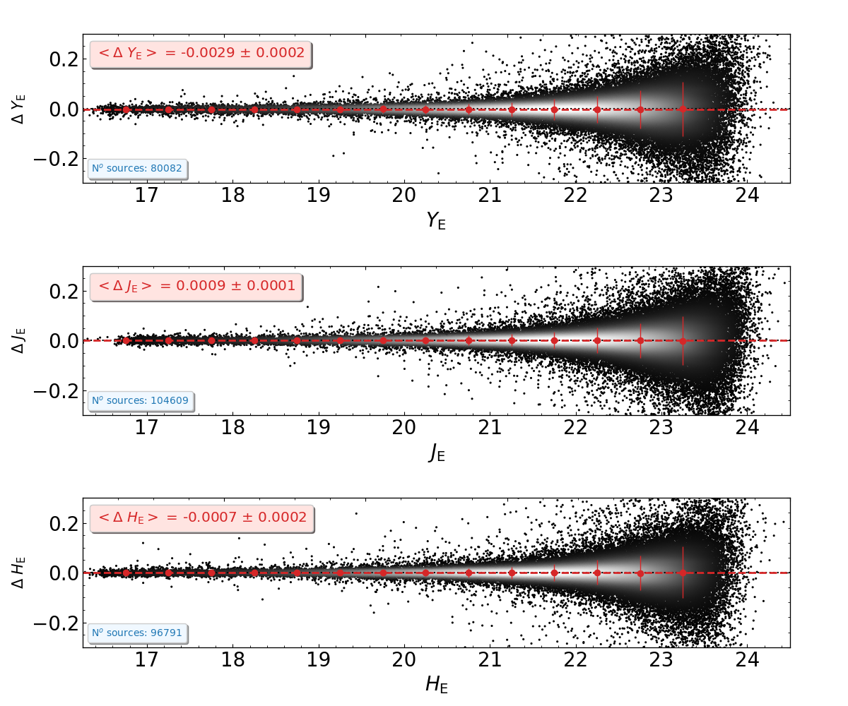
Figure 18: Photometric differences between July and August observations of the self-calibration field for the $Y_{\scriptscriptstyle\rm E}$, $J_{\scriptscriptstyle\rm E}$, and $H_{\scriptscriptstyle\rm E}$ bands. The plots illustrate the photometric stability.

6 Discussion and conclusions

This paper presents the NIR PF pipeline used to process NISP raw photometric exposures for Q1. While the calibrated images meet the key requirements for astrometric and photometric calibration, the DQC analysis and in-depth validation of the calibration products and images revealed certain limitations.

• Persistence signal. Unmasked residual streaks remain due to several factors, including the balance between masking unwanted features while preserving valid pixels and the accuracy of the model used to capture the complexities of detector physics behind persistence charges. Additionally, while masking can mitigate contamination from spectroscopic exposures on photometric ones, it cannot address persistence between consecutive photometric exposures taken at the same dither position. Persistence also impacts calibration products, such as small-scale and large-scale flats. An improved model is needed to enable an effective correction procedure, and is being worked on.

• PSF. An improved PSF model has been derived from observations of the self-calibration field, extending to larger radii and therefore providing a better characterisation of the extended PSF wings. The smaller PSF used for the Q1 processing reflects mainly on the quality of the PSF photometry in the Q1 catalogues, which is only available for bright sources.

• Background estimation. We noticed a positive correlation between the estimated background signal and the position of very bright objects, resulting in an over-subtraction in the outskirts of extended objects. This limits the accuracy of low-surface-brightness measurements on such targets, and also their detection.

• Some of the calibration products used for Q1 are based on ground calibration, and will be superseded by in-flight data in upcoming data releases.

• Unmodelled instrumental effects that are still to be fully treated. The DQC pipeline is based on metadata and statistics, and cannot fully capture the complexity of NIR images. Indeed a visual inspection performed on a subsample of the Q1 images revealed the presence of additional instrumental effects, such as diffuse arcs produced by internal reflections, affecting a very limited number of exposures. Due to the very low incidence of such artifacts, the development of a reliable model for these effects will take place on a timescale beyond Q1.

These issues are addressed in a new release of NIR PF for the preparation of DR1. This is scheduled for the end of 2025 within the Euclid Consortium, followed by a public release one year later.

Appendix A Constructing filter flats from LED flats

In general, a flat field at a 2-dimensional pixel position $\mathbf{x}$ and time $t$ can be written as

$${\rm FLAT_{Filter}}(\mathbf{x},t)=\int_{\lambda_{1}}^{\lambda_{2}}\mathrm{QE}(\lambda,\mathbf{x},t)\;T(\lambda,\mathbf{x},t)\;f_{\lambda}(\lambda,\mathbf{x},t)\;{\rm d}\lambda\;,$$ (15)

where QE is the quantum efficiency, $T$ is the filter (or dispersive element) transmission, and $f_{\lambda}$ is the spectral flux density of a flat-field lamp expressed per unit wavelength. While in theory the integration is over all wavelengths, in practice it can be bounded by some interval $[\lambda_{1},\lambda_{2}]$ that contains the bulk of the flux.

In the case of NISP, the QE varies little over the spectral range of interest, 0.9–2.2 $\mathrm{\SIUnitSymbolMicro m}$. The ideal lamp spectrum does not favour a particular wavelength, i.e. it produces the same number of photons per wavelength interval. In practice, as long as the S/N is sufficient at each wavelength while avoiding saturation, the exact shape of the lamp spectrum does not matter.

For NISP photometry, a lamp emitting the same number of photons per wavelength interval is desirable. The spectral flux density of the lamp is then

$$f_{\lambda}(\lambda,\mathbf{x},t)=f_{\lambda}^{0}(\mathbf{x},t)$$ (16)

with units photons s^-1 cm^-2 nm^-1. We chose these units because the provided spectral flux densities for the NISP LEDs have these units. The flat field itself then is

$${\rm FLAT_{Filter}}(\mathbf{x},t)=f_{\lambda}^{0}(\mathbf{x},t)\;\int_{\lambda_{1}}^{\lambda_{2}}\mathrm{QE}(\lambda,\mathbf{x},t)\;T(\lambda,\mathbf{x},t)\;{\rm d}\lambda\;.$$ (17)

The LEDs in NISP illuminate the focal plane array directly without passing through the filters or grisms. In the absence of these optical elements, the LED flat field can be written as

$${\rm FLAT_{\rm LED}}(\mathbf{x},t)=\int_{\lambda_{3}}^{\lambda_{4}}\mathrm{QE}(\lambda,\mathbf{x},t)\;f^{\rm LED}_{\lambda}(\lambda,\mathbf{x},t)\;{\rm d}\lambda\;,$$ (18)

where ${\rm FLAT_{\rm LED}}(\mathbf{x},t)$ is the observed LED flat, and $f^{\rm LED}_{\lambda}(\lambda,\mathbf{x},t)$ is the LED spectrum measured from the laboratory. The Cauchy mean value theorem states that for two continuous functions $f(x)$ and $g(x)$, with $g(x)\geq 0$ or $g(x)\leq 0$, one can always find a $x_{0}$ in the interval $[a,b]$ such that

$$\int_{a}^{b}g(x)\;f(x)\;{\rm d}x=f(x_{0})\;\int_{a}^{b}g(x)\;{\rm d}x\;.$$ (19)

This can be readily applied to Eq. 18 because QE is always positive and $f^{\rm LED}_{\lambda}$ is continuous (at least within the resolution limits of the measurements):

$${\rm FLAT_{\rm LED}}(\mathbf{x},t)=f^{\rm LED}_{\lambda}(\lambda_{0},\mathbf{x},t)\;\int_{\lambda_{3}}^{\lambda_{4}}\mathrm{QE}(\lambda,\mathbf{x},t)\;{\rm d}\lambda\;.$$ (20)

We can now solve Eq. 20 for $f^{\rm LED}_{\lambda}(\lambda_{0},\mathbf{x},t)$ and use it to replace $f_{\lambda}^{0}(\mathbf{x},t)$ in Eq. 17. This can be done because ${\rm FLAT_{Filter}}$ (and ${\rm FLAT_{LED}}$) are in the end subject to a global normalisation (chosen lamp brightness, normalisation to average unity, or else). We then have

$${\rm FLAT_{Filter}}(\mathbf{x},t)={\rm FLAT_{\rm LED}}(\mathbf{x},t)\;P(\mathbf{x},t)\;,$$ (21)

where

$$P(\mathbf{x},t)=\frac{\int_{\lambda_{1}}^{\lambda_{2}}\mathrm{QE}(\lambda,\mathbf{x},t)\;T(\lambda,\mathbf{x},t)\;{\rm d}\lambda}{\int_{\lambda_{3}}^{\lambda_{4}}\mathrm{QE}(\lambda,\mathbf{x},t)\;{\rm d}\lambda}$$ (22)

propagates the LED flat in wavelength to the bandpass $T$ of the filter in question. This propagation depends on pixel position $\mathbf{x}$, reflecting the spatially variably quantum efficiency as well as potential bandpass variations.

Appendix B Description of NIR PF data quality flags

We report for convenience the bit mask convention adopted for the NIR images from the Euclid Collaboration (2025).

Bit	Flag Name	Description	Invalid
0	INVALID	Convenience common flag
1	OBMASK	On-board flags
2	DISCONNECTED	Disconnected	Yes
3	ZEROQE	Zero QE	Yes
4	BADBASE	High or Low Baseline	Yes
5	LOWQE	QE ¡ 74% at 1120 $\leq$ $\lambda$/nm $\leq$ 2020 QE ¡ (64 + ($\lambda$/nm – 920)/20)% at 920 $\leq$ $\lambda$/nm $\leq$ 1120.
6	SUPERQE	Pixel QE ¿ 110%	Yes
7	HOT	Pixels with dark current signal falling 3 $\sigma$ above the detector median
8	RTN	Random Telegraph Noise	Yes
9	SNOWBALL	Very energetic internal deposit of signal in pixels	Yes
10	SATUR	Saturated Pixel	Yes
11	NLINEAR	Pixels whose signal in electrons are below or above the applicable signal limits
12	NLMODFAIL	Pixels whose linear correction model failed	Yes
13	PERSIST	Pixels affected by persistence charge from previous sources	Yes
14	PERMODFAIL	Pixels with persistence calibration procedure failed
15	DARKNODET	Pixels for which the dark current is not detected to within a maximum noise threshold
16	COSMIC	Cosmic ray hits	Yes
17	FLATLH	Pixels in the computed flat that have too low or too high response values
18	GHOST	Ghosts	Yes
19	SCATTER	Scattered Light
20	MOVING	Moving objects
21	TRANS	Transients
22	CROSSTALK	Cross Talk
23	FLOWER	‘Flower pixel’ found on MasterFlat	Yes
24	VIGNET	Pixels affected by vignetting on LED exposures

References

- Appleton et al. (2021) Appleton, P. N., Deustua, S. E., Scodeggio, M., et al. 2021, Cross-calibration of HST, Euclid and Roman grism/prism through WFC3-IR faint spectrophotometric white dwarf standards near the North and South Ecliptic Poles, HST Proposal. Cycle 29, ID. #16702
- Barbier et al. (2018) Barbier, R., Buton, C., Clemens, J. C., et al. 2018, in SPIE Conf. Ser., Vol. 10709, High Energy, Optical, and Infrared Detectors for Astronomy VIII, ed. A. D. Holland & J. Beletic, 107090S
- Bertin (2006) Bertin, E. 2006, in ASP Conf. Ser., Vol. 351, Astronomical Data Analysis Software and Systems XV, ed. C. Gabriel, C. Arviset, D. Ponz, & S. Enrique, 112
- Bertin (2011) Bertin, E. 2011, in Astronomical Society of the Pacific Conference Series, Vol. 442, Astronomical Data Analysis Software and Systems XX, ed. I. N. Evans, A. Accomazzi, D. J. Mink, & A. H. Rots, 435
- Bertin & Arnouts (1996) Bertin, E. & Arnouts, S. 1996, A&AS, 117, 393
- Bohlin et al. (2024) Bohlin, R. C., Deustua, S., Narayan, G., et al. 2024, AJ, 169, 40
- Bohlin et al. (2014) Bohlin, R. C., Gordon, K. D., & Tremblay, P. E. 2014, PASP, 126, 711
- Bohlin et al. (2020) Bohlin, R. C., Hubeny, I., & Rauch, T. 2020, AJ, 160, 21
- Bohlin et al. (2017) Bohlin, R. C., Mészáros, S., Fleming, S. W., et al. 2017, AJ, 153, 234
- Calabretta & Greisen (2002) Calabretta, M. R. & Greisen, E. W. 2002, A&A, 395, 1077
- Cogato et al. (2024) Cogato, F., Medinaceli Villegas, E., Barbier, R., et al. 2024, in SPIE Conf. Ser., Vol. 13092, Space Telescopes and Instrumentation 2024: Optical, Infrared, and Millimeter Wave, ed. L. E. Coyle, S. Matsuura, & M. D. Perrin, 130923G
- Copin (2022) Copin, Y. 2022, Outlier detection in small samples using pull-clipping, https://ycopin.pages.in2p3.fr/inSpec/outliers.html
- Deustua et al. (2023) Deustua, S. E., Appleton, P. N., Bohlin, R. C., Schirmer, M., & Tremblay, P.-E. 2023, Calibrating the Universe: Faint White Dwarf Standard Stars at the Ecliptic Poles for Cross-calibration of HST, Euclid and Roman, HST Proposal. Cycle 31, ID. #17442
- Euclid Collaboration (2025) Euclid Collaboration. 2025, Euclid SGS Data Product Description Document - NIR, https://euclid.esac.esa.int/msp/dpdd/v1.1/nirdpd/nirindex.html
- Euclid Collaboration: Aussel et al. (2025) Euclid Collaboration: Aussel, H., Tereno, I., Schirmer, M., et al. 2025, A&A, submitted
- Euclid Collaboration: Castander et al. (2024) Euclid Collaboration: Castander, F., Fosalba, P., Stadel, J., et al. 2024, A&A, accepted, arXiv:2405.13495
- Euclid Collaboration: Copin et al. (2025) Euclid Collaboration: Copin, Y., Fumana, M., Mancini, C., et al. 2025, A&A, submitted
- Euclid Collaboration: Cropper et al. (2024) Euclid Collaboration: Cropper, M., Al Bahlawan, A., Amiaux, J., et al. 2024, A&A, accepted, arXiv:2405.13492
- Euclid Collaboration: Hormuth et al. (2024) Euclid Collaboration: Hormuth, F., Jahnke, K., Schirmer, M., et al. 2024, A&A, accepted, arXiv:2405.13494
- Euclid Collaboration: Jahnke et al. (2024) Euclid Collaboration: Jahnke, K., Gillard, W., Schirmer, M., et al. 2024, A&A, accepted, arXiv:2405.13493
- Euclid Collaboration: McCracken et al. (2025) Euclid Collaboration: McCracken, H., Benson, K., et al. 2025, A&A, submitted
- Euclid Collaboration: Mellier et al. (2024) Euclid Collaboration: Mellier, Y., Abdurro’uf, Acevedo Barroso, J., et al. 2024, A&A, accepted, arXiv:2405.13491
- Euclid Collaboration: Romelli et al. (2025) Euclid Collaboration: Romelli, E., Kümmel, M., Dole, H., et al. 2025, A&A, submitted
- Euclid Collaboration: Scaramella et al. (2022) Euclid Collaboration: Scaramella, R., Amiaux, J., Mellier, Y., et al. 2022, A&A, 662, A112
- Euclid Collaboration: Schirmer et al. (2022) Euclid Collaboration: Schirmer, M., Jahnke, K., Seidel, G., et al. 2022, A&A, 662, A92
- Euclid Collaboration: Schirmer et al. (2023) Euclid Collaboration: Schirmer, M., Thürmer, K., Bras, B., et al. 2023, A&A, 675, A142
- Euclid Quick Release Q1 (2025) Euclid Quick Release Q1. 2025, https://doi.org/10.57780/esa-2853f3b
- Gaia Collaboration et al. (2023) Gaia Collaboration, Vallenari, A., Brown, A. G. A., et al. 2023, A&A, 674, A1
- Grupp et al. (2019) Grupp, F., Kaminski, J., Bodendorf, C., et al. 2019, in SPIE Conf. Ser., Vol. 11116, Astronomical Optics: Design, Manufacture, and Test of Space and Ground Systems II, ed. T. B. Hull, D. W. Kim, & P. Hallibert, 1111618
- Hildebrand (1956) Hildebrand, F. B. 1956, Introduction to numerical analysis, International Series in Pure and Applied Mathematics (New York: McGraw-Hill)
- Kubik et al. (2014) Kubik, B., Barbier, R., Castera, A., et al. 2014, in SPIE Conf. Ser., Vol. 9154, High Energy, Optical, and Infrared Detectors for Astronomy VI, ed. A. D. Holland & J. Beletic, 91541B
- Kubik et al. (2016) Kubik, B., Barbier, R., Chabanat, E., et al. 2016, PASP, 128, 104504
- Kubik et al. (2024) Kubik, B., Barbier, R., Smadja, G., et al. 2024, in X-Ray, Optical, and Infrared Detectors for Astronomy XI, ed. A. D. Holland & K. Minoglou, Vol. 13103, SPIE, 1310315
- Le Graët et al. (2022) Le Graët, J., Secroun, A., Barbier, R., et al. 2022, in Society of Photo-Optical Instrumentation Engineers (SPIE) Conference Series, Vol. 12191, X-Ray, Optical, and Infrared Detectors for Astronomy X, ed. A. D. Holland & J. Beletic, arXiv:2209.01831
- Leisenring et al. (2016) Leisenring, J. M., Rieke, M., Misselt, K., & Robberto, M. 2016, in High Energy, Optical, and Infrared Detectors for Astronomy VII, ed. A. D. Holland & J. Beletic, Vol. 9915, SPIE, 99152N
- Massey & Refregier (2005) Massey, R. & Refregier, A. 2005, MNRAS, 363, 197
- Medinaceli et al. (2020) Medinaceli, E., Farinelli, R., Balestra, A., et al. 2020, in SPIE Conf. Ser., Vol. 11443, Space Telescopes and Instrumentation 2020: Optical, Infrared, and Millimeter Wave, ed. M. Lystrup & M. D. Perrin, 1144359
- Medinaceli et al. (2022) Medinaceli, E., Valenziano, L., Auricchio, N., et al. 2022, in SPIE Conf. Ser., Vol. 12180, Space Telescopes and Instrumentation 2022: Optical, Infrared, and Millimeter Wave, ed. L. E. Coyle, S. Matsuura, & M. D. Perrin, 121801L
- Molinari et al. (2011) Molinari, S., Schisano, E., Faustini, F., et al. 2011, A&A, 530, 10
- Morris & Kubik (2022) Morris, P. W. & Kubik, B. 2022, Euclid SGS NIR Common Pipeline Flags, Euclid Collaboration Document, Technical Report, EUCL-IPA-TN-8-001 issue 0.9, 2022 April 4
- Narayan et al. (2019) Narayan, G., Matheson, T., Saha, A., et al. 2019, ApJS, 241, 20
- Plazas et al. (2017) Plazas, A. A., Shapiro, C., Smith, R., Rhodes, J., & Huff, E. 2017, Journal of Instrumentation, 12, C04009
- Rauscher et al. (2019) Rauscher, B. J., Arendt, R. G., Fixsen, D. J., et al. 2019, Journal of Astronomical Telescopes, Instruments, and Systems, 5, 028001
- Rauscher et al. (2014) Rauscher, B. J., Boehm, N., Cagiano, S., et al. 2014, PASP, 126, 739
- Reiss (1945) Reiss, M. 1945, J. Opt. Soc. Am., 35, 283
- Shupe et al. (2012) Shupe, D. L., Laher, R. R., Storrie-Lombardi, L., et al. 2012, in SPIE Conf. Ser., Vol. 8451, Software and Cyberinfrastructure for Astronomy II, ed. N. M. Radziwill & G. Chiozzi, 84511M
- Shupe et al. (2005) Shupe, D. L., Moshir, M., Li, J., et al. 2005, in ASP Conf. Ser., Vol. 347, Astronomical Data Analysis Software and Systems XIV, ed. P. Shopbell, M. Britton, & R. Ebert, 491
- Smith et al. (2008) Smith, R. M., Zavodny, M., Rahmer, G., & Bonati, M. 2008, in SPIE Conf. Ser., Vol. 7021, High Energy, Optical, and Infrared Detectors for Astronomy III, ed. D. A. Dorn & A. D. Holland, 70210J
- Tulloch (2018) Tulloch, S. 2018, Scientific Detector Workshop 2017, Baltimore, arXiv:1807.05217
- Vacca et al. (2004) Vacca, W. D., Cushing, M. C., & Rayner, J. T. 2004, PASP, 116, 352
- van Dokkum (2001) van Dokkum, P. G. 2001, PASP, 113, 1420