Euclid Quick Data Release (Q1)

The first Euclid Quick Data Release, Q1, comprises 63.1 deg² of the Euclid Deep Fields (EDFs) to nominal wide-survey depth. It encompasses visible and near-infrared space-based imaging and spectroscopic data, ground-based photometry in the $u$, $g$, $r$, $i$, and $z$ bands, as well as corresponding masks. Overall, Q1 contains about 30 million objects in three areas near the ecliptic poles around the EDF-North and EDF-South, as well as the EDF-Fornax field in the constellation of the same name. The purpose of this data release – and its associated technical papers – is twofold. First, it is meant to inform the community of the enormous potential of the Euclid survey data, to describe what is contained in these data, and to help prepare expectations for the forthcoming first major data release DR1. Second, it enables a wide range of initial scientific projects with wide-survey Euclid data, ranging from the early Universe to the Solar System. The Q1 data were processed with early versions of the processing pipelines, which already demonstrate good performance, with numerous improvements in implementation compared to pre-launch development. In this paper, we describe the sky areas released in Q1, the observations, a top-level view of the data processing of Euclid and associated external data, the Q1 photometric masks, and how to access the data. We also give an overview of initial scientific results obtained using the Q1 data set by Euclid Consortium scientists, and conclude with important caveats when using the data. As a complementary product, Q1 also contains observations of a star-forming area in Lynd’s Dark Nebula 1641 in the Orion A Cloud, observed for technical purposes during Euclid’s performance-verification phase. This is a unique target, of a type not commonly found in Euclid’s nominal sky survey.

1 Introduction

Euclid is a space mission of the European Space Agency (ESA) with the primary goal of studying dark matter and dark energy using two main probes, weak gravitational lensing and galaxy clustering (Euclid Collaboration: Mellier et al. 2024). Euclid uses a 1.2-m diameter Korsch telescope with a field of view of 0.54 deg², imaged by two instruments, VIS (Euclid Collaboration: Cropper et al. 2024) and the Near-Infrared Spectrometer and Photometer (NISP; Euclid Collaboration: Jahnke et al. 2024), with the mission of conducting the Euclid Wide Survey (EWS), covering 14 000 deg² of the extragalactic sky (Euclid Collaboration: Scaramella et al. 2022). VIS is a broad-band optical imager with a spatial resolution of $0.\mathrm{″}18$, designed to measure the distortion of galaxy shapes with $I_{\scriptscriptstyle\rm E}\lesssim 24.5$. NISP combines the capabilities of an imager in the near-infrared (NIR) bands $Y_{\scriptscriptstyle\rm E}$, $J_{\scriptscriptstyle\rm E}$, and $H_{\scriptscriptstyle\rm E}$ (Euclid Collaboration: Schirmer et al. 2022) to derive the photometric redshifts of the galaxies whose shapes are measured with VIS, together with a near-infrared slitless spectrograph to measure accurate redshifts of galaxies with bright emission lines.

The VIS single $I_{\scriptscriptstyle\rm E}$ band is too wide to allow for the determination of the photometric redshifts of the objects whose shapes are being measured. To this end, the Euclid space data are combined with ground-based photometry in the u, g, r, i, and z bands from large-area surveys. In the southern sky, the Dark Energy Survey (DES; Abbott et al. 2021) is currently used until deeper data from the Vera C. Rubin Observatory (Ivezić et al. 2019) become available. In the northern sky, a new collaboration has been set up, the Ultraviolet Near-Infrared Optical Northern Survey (UNIONS; Gwyn et al., in prep.), with the aim to survey the sky in the ugriz bands. This is a joint effort between the Canada-France Imaging Survey (CFIS; Ibata et al. 2017) for the u and r bands, the Panchromatic Survey Telescope and Rapid Response System (Pan-STARRS; Chambers et al. 2016) for the i band, and the Subaru Hyper Suprime Camera (HSC; Miyazaki et al. 2018) for both the g band, through the Waterloo-Hawaii-IfA g-band Survey (WHIGS, PIs K. C. Chambers and M. J. Hudson), and the z band, through the Wide Imaging with Subaru-Hyper Suprime-Cam Euclid Sky survey (WISHES, PI M. Oguri). In the Euclid project, we refer to these external data as ‘EXT’. They are ingested and recalibrated to a flux scale in common with the VIS and NISP data. Together, the space- and ground-based data form the Euclid mission data set.

In addition to the main survey, a significant fraction of observational time is spent on specific fields that, thanks to repeated visits, will accumulate greater depth than the EWS, up to a gain of about two magnitudes (Euclid Collaboration: Mellier et al. 2024). These are the Euclid Deep Fields and the Euclid Auxiliary Fields, supporting our instrument calibration and characterising the source population (Scaramella et al., in prep.).

Nominal EWS observations started on 14 February 2024. It will take Euclid 6 years to collect all of its 14 000 deg² and associated Euclid Deep Survey (EDS). The project foresees three major data releases of the survey data, DR1 to DR3, with DR1 using the first year of data collected, DR2 the first three years, and DR3 occurring after all survey observations have ended. The internal and public releases of DR1 are scheduled for October 2025 and 2026, respectively. A special data release, Q1, aimed at giving a taste of the capacities of the Euclid mission to the astronomical community was planned to take place 14 months after the start of the survey. The fields to be included in the release were to be the three EDFs and other areas of interests. The area of Q1 is not large enough to allow meaningful derivation of cosmological parameters, but it is large enough for a slew of non-cosmological studies, as testified by the more than 30 publications from consortium members based on this release.

In Sect. 2 we present the sky fields that comprise Q1, and Sect. 3 contains a summary of the associated Euclid and ground-based EXT observations. Overviews of the Euclid mission data processing are given in Sect. 4, with details expanded in separate papers, and in Sect. 5 for the EXT data. The survey masks are discussed in Sect. 6, and data access is outlined in Sect. 7. We conclude with a presentation of various scientific results enabled by the Q1 data release in Sect. 8 and discuss a few important caveats to bear in mind while using the data in Sect. 9.

All Euclid magnitudes are in the physical AB system (Oke & Gunn 1983), the astrometric calibration is against Gaia DR3 (Gaia Collaboration et al. 2023), and the photometric calibration against the Hubble Space Telescope (HST) CALSPEC database (see e.g., Bohlin et al. 2020).

2 Q1 sky content

2.1 Euclid Deep Fields

The 63.1 deg² of Q1 comprise observations of the Euclid Deep Field North (EDF-N), Euclid Deep Field South (EDF-S), and Euclid Deep Field Fornax (EDF-F) – see Table 1 – to the single-visit depth of the EWS. They provide a preview of the typical depth expected across most of the Euclid survey. By DR3 the EDFs will have been observed multiple times, reaching 2 mag deeper than the EWS over an area of 53 deg² (Euclid Collaboration: Mellier et al. 2024). The total number of visits to each EDF is adjusted to the different levels of zodiacal background present at the location of each field to reach a uniform depth at DR3. Each EDF visit consists of a so-called ‘patch’ of reference observing sequences, the building block of the EWS (Euclid Collaboration: Scaramella et al. 2022). The tiling of a patch places the ROSs side-by-side with some overlap. Each visit covers the full deep field counting toward 53 deg². A margin is needed because of the varying position angle from the orbit progression and the tiling itself, resulting in the additional 10 deg² for Q1.

The EWS and EDS differ concerning the NISP spectroscopic observations. While the EWS is exclusively observed with the ‘red grism’ (${\rm RG}_{\scriptscriptstyle\rm E}$, 1206–1892 $\mathrm{\SIUnitSymbolMicro m}$), the EDFs are also observed with the ‘blue grism’ (${\rm BG}_{\scriptscriptstyle\rm E}$, 926–1366 $\mathrm{\SIUnitSymbolMicro m}$), maintaining an approximate blue-to-red exposure-time ratio of 5:3. This enables the construction of a pure and complete spectroscopic reference sample of galaxies. The EDF observations selected for Q1 are all made with the red grism.

The main EDF properties are summarised in Table 1. EDF-N is an ecliptic-polar field with a circular shape covering 20 deg² to full depth by DR3. This field has the lowest zodiacal background, but it also has a lower Galactic latitude and thus a somewhat higher stellar density, extinction, and reddening. Because this field is always visible, it can be observed with a wide spread of position angles throughout the year. This strategy yields the diversity of spectral directions needed to build the complete and pure spectroscopic reference sample; the EDF-N Q1 data correspond to one particular orientation. EDF-S is at a lower ecliptic latitude with two relatively long visibility windows per year, meaning that the range of position angles is restricted compared to that of EDF-N. It has a stadium shape, encompassing two tangent circles each covering 10 deg², with a total coverage of 23 deg². The EDF-F covers a 10 deg² circular region centred on the Chandra Deep Field South (CDFS), a location with a considerable amount of multi-wavelength data that is easily accessible from ground-based observatories; for Euclid it has two short visibility windows per year. Figure 12 shows the EDF sky footprints of the Q1 visits. The footprints are reproduced in Appendix A as standard-format region files. Figure 1 zooms in the three EDF areas showing information on sky quality and coverage by other surveys.

Table 1: Summary of the properties of the EDFs. We list the Q1 area, and the smaller area in DR3 that reaches full target depth. Here $\lambda$ and $\beta$ refer to ecliptic longitude and latitude, respectively.

Field	Q1 area	DR3-depth area	RA	Dec	$\lambda$	$\beta$	DR3 visits
EDF-N	22.9 ${\rm deg^{2}}$	20 ${\rm deg^{2}}$	$269.\mathrm{°}733$	$-$$66.\mathrm{°}018$	$258.\mathrm{°}690$	$-$$89.\mathrm{°}446$	40
EDF-S	28.1 ${\rm deg^{2}}$	23 ${\rm deg^{2}}$	0$61.\mathrm{°}241$	$-48.\mathrm{°}423$	0$36.\mathrm{°}493$	$-66.\mathrm{°}599$	45
EDF-F	12.1 ${\rm deg^{2}}$	10 ${\rm deg^{2}}$	0$52.\mathrm{°}932$	$-28.\mathrm{°}088$	0$40.\mathrm{°}772$	$-45.\mathrm{°}397$	52

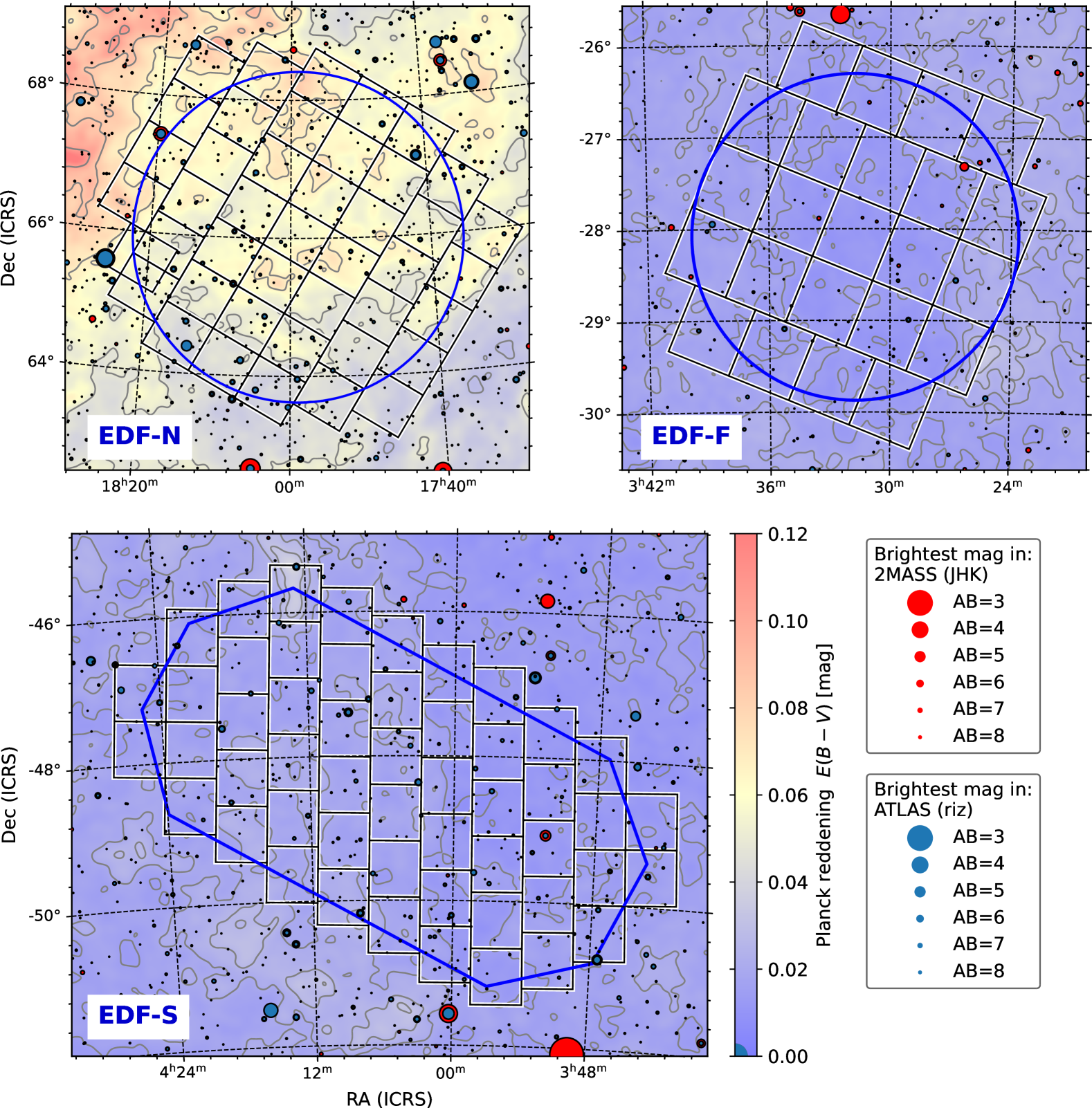
Figure 1: Layout of the three EDF tilings comprising Q1 (black squares), overlaid on the reddening map from Planck Collaboration XI (2014), with bright stars from 2MASS (Skrutskie et al. 2006) and ATLAS-Refcat2 (Tonry et al. 2018). The thick blue lines show the approximate areas that will be covered to full depth by DR3.

2.2 LDN 1641 in the Orion A Cloud

Euclid’s fine-guidance sensor (FGS) comprises four charge-coupled devices adjacent to the VIS detectors, observing in the same 530–920 nm $I_{\scriptscriptstyle\rm E}$ passband as VIS itself. To test and further optimise the performance of the FGS in September 2023, two months after launch, we needed to observe an area that had a particularly low number density of suitable guide stars. Because of thermal constraints, Euclid can observe within a narrow meridian circle only (Euclid Collaboration: Scaramella et al. 2022). The only suitable area visible at that time, where all FGS detectors would see very low guide-star densities, was a part of Lynd’s Catalogue of Dark Nebulae (LDN) 1641 (Lynds 1962), an extended dust-obscured part of the Orion A Cloud. We refer to this area observed by Euclid as the ‘dark cloud’, centred near ${\rm RA}={$$}$ and ${\rm Dec}=$$$ (see Fig. 2). Euclid observed a single field of view in the dark cloud area, i.e., approximately 0.5 deg².

This star-forming area is known for its young stellar objects (YSOs, e.g. Fang et al. 2009, 2013; Roquette et al. 2025), predominantly becoming visible at wavelengths above 1 $\mathrm{\SIUnitSymbolMicro m}$. There are targeted near-infrared HST observations of protostars (programme ID 11548, Megeath 2007) that were used, for example, by Habel et al. (2021). The area was catalogued as part of the Herschel Orion Protostar Survey (HOPS, Furlan et al. 2016), facilitating far-infrared studies (e.g. Fischer et al. 2020), and was mapped at sub-millimetre wavelengths by the Atacama Large Millimeter/Submillimeter Array (Grant et al. 2021).

The dust extinction in the area ranges from 2 to at least 19 mag in $R$-band (Schlafly & Finkbeiner 2011), with a typical value of about 7–8 mag that reduces to about 2 to 1 mag at wavelengths of 1 and 2 $\mathrm{\SIUnitSymbolMicro m}$, respectively. Accordingly, the VIS data reveal comparatively little, whereas NISP shows an unprecedented, wide and contiguous view of the embedded objects in their larger environment.

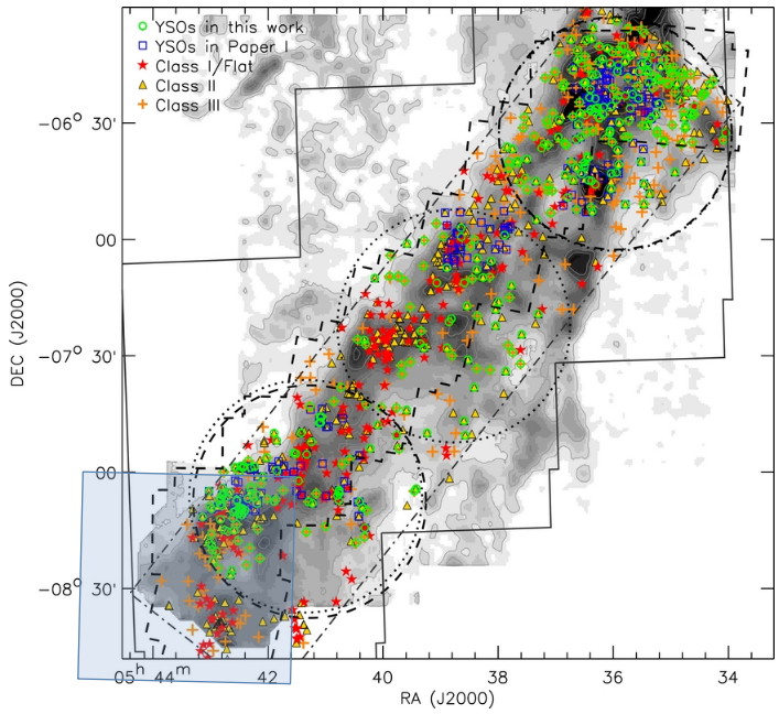
Figure 2: Map of YSOs in the Orion A Cloud (adapted from Fang et al. 2013). The markers show the various object classes, superimposed on a grey-scale ^13CO emission map. The large blue square in the bottom-left corner marks the Euclid observations, comprising about 100 YSOs.

2.3 Target populations

With 63.1 deg², the Q1 area coverage is likely to be comparable within a factor of a few to that of HST since its launch. While the range of astrophysical targets in Q1 is naturally smaller than HST’s, due to the restricted instrument suite onboard Euclid and because of Euclid’s preferred sky areas, it is nonetheless considerable. Aside from tens of millions of galaxies the data comprise, for example, three extended planetary nebulae: PN K 1-16 (Kohoutek 1963; Montez & Kastner 2013) and the well-known Cat’s Eye Nebula (NGC 6543), both in the EDF-N; and the little-studied Robin’s Egg Nebula (NGC 1360; see also Goldman et al. 2004; Garc´ıa-D´ıaz et al. 2008) in EDF-F. The Q1 data of NGC 1360 are arguably the best images ever taken of it, resolving numerous cometary globules and showing the two bipolar jets in great detail. However, we note that our pipelines have an active background subtraction geared toward cosmological science. Therefore, extended nebulosity and low-surface brightness features such as tidal tails, galactic haloes, and intra-cluster light are either suppressed, removed, or over-corrected in the stacked Q1 images (see also Euclid Collaboration: McCracken et al. 2025; Euclid Collaboration: Polenta et al. 2025; Euclid Collaboration: Romelli et al. 2025). Notably, the EDF-N contains the Euclid self-calibration field, which will eventually become the deepest Euclid field, with many hundreds of visits. The self-calibration field contains our recently published Einstein ring around the nucleus of NGC 6505 (O’Riordan et al. 2025).

3 Observations

3.1 Selection of the Q1 observations of the EDF areas

The criteria for the selection of the single pass of each EDF for Q1 were as follows. First, the pass had to be observed using the red grism to reproduce the observations of the EWS. Second, the data set had to be as complete as possible, meaning no instrument failure during observations, and absence of high Solar activity for optimal data quality. Third, the pass had to be observed shortly after Euclid’s second decontamination campaign for maximum photometric stability. Lastly, the visit had to occur in time for the planned reprocessing campaign in October 2024.

For the EDF-F, only two passes were available, one with the blue grism and one with the red (patch 59). The latter was obtained between 2024-08-05T20:56Z and 2024-08-07T00:55Z, and matched all our criteria. For the EDF-N, out of six available passes with the red grism, one was lost to high Solar activity and another was acquired with heavy ice contamination on one of the mirrors (Euclid Collaboration: Schirmer et al. 2023). Among the remaining four, we selected the one with the least data loss to cosmic rays, patch 49, obtained between 2024-07-17T16:06Z and 2024-07-19T20:43Z. For the EDF-S, we used patch 71, observed between 2024-09-05TT13:52Z and 2024-09-08T05:34Z, which was preferred over two other passes because of low Solar activity.

All selected passes were executed after Euclid’s second thermal decontamination on 8 June 2024 to remove water ice, restoring a largely stable throughput since then. The associated self-calibration observations to infer uniform relative photometric calibration at the level of a few millimag, and absolute calibration at the level of 1%, were taken on 19 June 2024, 19 July 2024, 23 August 2024, and 29 September 2024.

Further calibration products, such as biases, darks, lamp flats, nonlinearity, distortion, spectral traces, and wavelength calibration, are based on a large number of observations with varying cadences from Euclid’s routine calibration plan and performance-verification (PV) phase. They were selected to provide the best match for the Q1 data. It is beyond the scope of this paper to describe this process in detail. More information about the calibration is given in the technical papers complementing Q1 (see also Sect. 4).

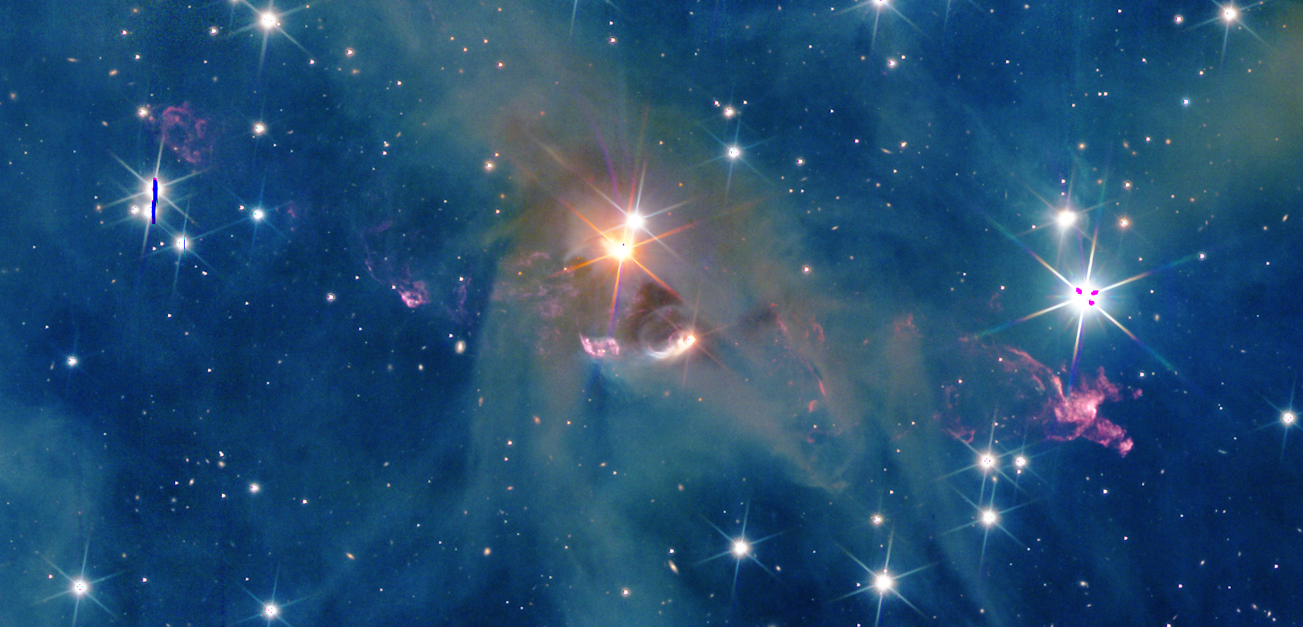
Figure 3: Small cutout of the NISP dark-cloud image. Shown near the centre is HOPS 221, a YSO with prominent outflows that can be traced across the image and beyond. North is up, east is to the left, and the field is $7\mathrm{\prime }$ wide.

3.2 Dark-cloud observations

The dark-cloud data included in Q1 were observed using the ROS on September 24 and 27, 2023, using three different roll angles of ${\rm AA}=-5.5$, $-6.5$, and $-7.5$ (see Euclid Collaboration: Mellier et al. 2024, for spacecraft angles). The slitless spectra were not processed by the pipeline due to the extended, rich nebulosity, and are therefore not available for this particular field.

In total, 68 and 34 nominal and short-science exposures were taken with VIS, for a total of 41 140 s or 17 times the EWS exposure time. However, due to the heavy dust extinction along this line of sight (Sect. 2.2), the VIS data do not reveal much. 68 exposures were also taken in each of the $Y_{\scriptscriptstyle\rm E}$, $J_{\scriptscriptstyle\rm E}$, and $H_{\scriptscriptstyle\rm E}$ bands, for a total of 5930 s per band using the standard NISP imaging mode. The NISP data also comprise 17 times the exposure time of the EWS and thus – in the absence of shot-noise from foreground emission – the $5\,\sigma$ point-source depth would be expected to be about 1.5 mag deeper than that of the EWS, or about 25.9 mag in each band. Figure 3 shows a small cut-out of the NISP data centred on HOPS 221.

3.3 Ground-based observations

The EDFs are the target of dedicated deep ground-based observations. The EDF-N is one of the targets of the Cosmic Dawn Survey (Euclid Collaboration: McPartland et al. 2024), gathering MegaCam $u$ and Subaru Hyper Suprime Camera (HSC) $g$, $r$, $i$, $z$, and $y$ imaging together with Spitzer/IRAC 3.6 $\mathrm{\SIUnitSymbolMicro m}$ and 4.5 $\mathrm{\SIUnitSymbolMicro m}$ data. The EDF-F and EDF-S sit in Vera C. Rubin Observatory’s Legacy Survey of Space and Time (LSST) footprint (Ivezić et al. 2019) and will accumulate deep data over the course of its mission. Moreover, EDF-F is one of the Vera C. Rubin Observatory’s deep-drilling fields. All these will be at least two magnitudes deeper than the EWS EXT data, and will be ideal for fully exploiting the final EDFs data accumulated in the course of the mission.

For Q1 our goal is to demonstrate the potential of the EWS, and therefore we use observations from the EXT data set that overlap with the EDFs locations and are representative of the EWS depth over the Euclid region of interest (ROI). For EDF-N we use data collected by the Ultraviolet Near-Infrared Optical Northern Survey (UNIONS) survey (Gwyn et al., in prep.), a collaboration of wide-field imaging surveys of the northern sky obtained using facilities in Hawai’i. They provide $u$ and $r$ band imaging using MegaCam (Boulade et al. 1998) at the 3.6-m Canada–France–Hawaii Telescope (CFHT) on Maunakea, $g$ and $z$ band imaging with HSC (Miyazaki et al. 2018) mounted on the Subaru 8.2-m telescope and $i$ band imaging from Pan-STARRS on Haleakala. All these data are delivered fully reduced, astrometrically calibrated and with an initial photometric calibration. For EDF-F and EDF-S, we use data taken largely by the Dark Energy Survey (DES) (Abbott et al. 2021) but supplemented with additional DECam (Flaugher et al. 2015) observations obtained by a variety of projects. These raw exposures in the $g$, $r$, $i$, and $z$ bands are then detrended and astrometrically and photometrically calibrated by the Euclid collaboration as described below in Sect. 5. As part of that ‘Euclidisation’ of these heterogeneous datasets, the UNIONS and DES data sets are photometrically calibrated as described below using the exquisite Gaia spectrophotometry.

4 Data processing

The Euclid mission data are processed by the Science Ground Segment (SGS), a distributed system across ten Science Data Centres in Europe and the United States. The SGS executes a pipeline chaining together different processing functions and producing various products. The Q1 pipeline is outlined in Fig. 4, where the various data products and PFs are identified. In this section, we present a very top-level view of the SGS pipeline only, and for details refer to the individual papers that describe the various PFs.

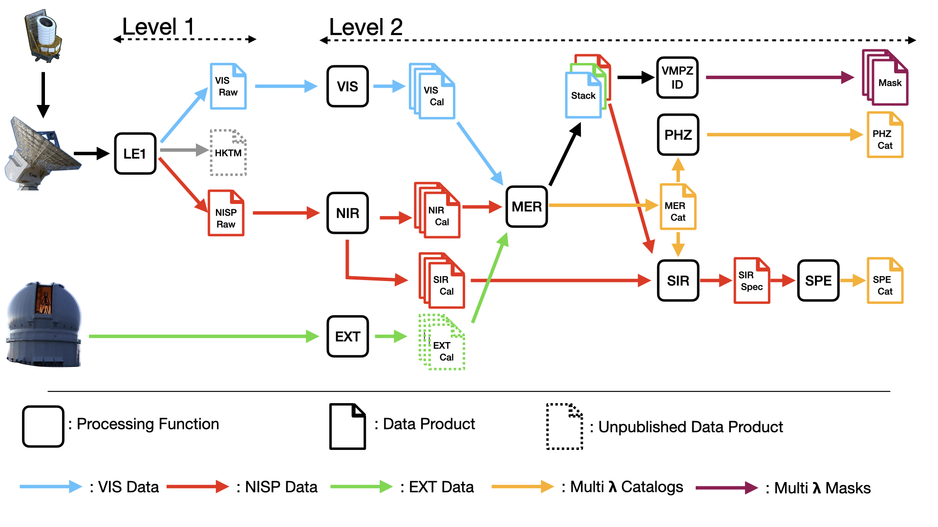
Figure 4: Overview of the Q1 data processing, showing the main data products making up the Q1 data release, together with the SGS PFs creating them, and outlining the flow of the various data sets. ‘Raw’ products refer to products created from the decommuted telemetry without any further processing. ‘Cal’ products refer to calibrated data, with instrument signatures being removed and data put on a physical scale. ‘Stack’ refers to image combinations, ‘Spec’ to combined 1D spectra, and ‘Cat’ to catalogues.

4.1 Telemetry decommutation

Decommutation is the process of extracting and reconstructing individual data streams from a time-multiplexed signal, typically in telemetry systems used for spacecraft communication. First, the telemetry from the Euclid satellite is received daily at ESA’s mission operation centre (MOC) located at the European Science Operations Centre (ESOC) in Darmstadt, Germany. It is then transferred to the Science Operations Centre (SOC) at the European Space Astronomy Centre (ESAC) in Spain. Telemetry consists of VIS and NISP detector data, together with VIS, NISP, and spacecraft housekeeping data, as well as MOC auxiliary products. It is transformed by the ‘LE1’ PF into the three Level 1 (LE1) products that are the inputs to the SGS pipeline: the VIS raw-frame product, the NISP raw-frame product, and the housekeeping telemetry (HKTM) product. The Q1 processing of the VIS data uses only VIS raw frames, and the NISP processing of both images and spectra uses only the NISP raw-frame products.

These raw-frame products are distributed in Q1 and are described in detail in the Data Product Description Document (DPDD). They are the starting point of the SGS data processing. Information from the HKTM product is used for the precise reconstruction of the VIS point-spread function (PSF), taking into account the satellite’s attitude variation during an observation. This will be used in the first data release (DR1) for accurate weak-lensing measurements, which are not part of Q1. Hence the HKTM product is not distributed in Q1. For completeness, we could not include the numerous calibration products with accurate descriptions of their validity ranges and the way they have to be applied to the data. This is well outside the scope and purpose of Q1.

4.2 Calibration and stacking

The LE1 products are then distributed among the remaining nine SDCs, according to their position on the celestial sphere, in order to be fully processed into LE2 products. This separation is required in order to minimise the amount of data transfer between SDCs during the processing.

The VIS data are processed by the VIS PF (Euclid Collaboration: McCracken et al. 2025), delivering single-frame calibrated images in the $I_{\scriptscriptstyle\rm E}$ band, together with associated catalogues. Moreover, VIS PF produces stacked images of the six frames collected during a ROS, that is four nominal science exposures of 560 s integration time and two short ones with 90 s; these stacks are not included in Q1. The NISP imaging data are processed by the NIR PF, delivering single calibrated frames in the $Y_{\scriptscriptstyle\rm E}$, $J_{\scriptscriptstyle\rm E}$, and $H_{\scriptscriptstyle\rm E}$ bands, together with associated catalogues (Euclid Collaboration: Polenta et al. 2025). The associated ground-based imaging data are processed by the EXTernal data (EXT) PF detailed in Sect. 5.

The VIS, NIR, and EXT data available on a survey tile are then collected by the MERge datasets (MER) PF that proceeds to build combined stacks per band, and creates a master catalogue selected in both the $I_{\scriptscriptstyle\rm E}$-band and in a combined $Y_{\scriptscriptstyle\rm E}$ + $J_{\scriptscriptstyle\rm E}$ + $H_{\scriptscriptstyle\rm E}$ detection stack. MER PF provides a large number of photometric and morphology measurements for each source, presented in detail in Euclid Collaboration: Romelli et al. (2025). The Sérsic morphology measurements are further discussed in Euclid Collaboration: Quilley et al. (2025). The MER stacks contain, for each tile, root mean square (RMS) and flag maps at the scale of 0$\aas@@fstack{\prime\prime}$1 for VIS and NIR (Euclid Collaboration: Polenta et al. 2025). These are combined into coarser masks over the entire data release to allow for statistical quantities to be derived by the VMPZ-ID PF (see Sect. 6).

4.3 Further catalogue and spectra extraction

The MER photometric information is used by the PHotometric redshift (PHZ) PF to determine the type, photometric redshift if applicable, and physical properties of each source. This step is described in Euclid Collaboration: Tucci et al. (2025).

Spectra of all sources detected at $H_{\scriptscriptstyle\rm E}\leq 22.5$ are extracted from the NISP spectroscopic exposures by the SIR-PF to provide calibrated spectra, as described in Euclid Collaboration: Copin et al. (2025). These are used by the SPEctroscopy (SPE) PF to measure redshifts and lines fluxes (Euclid Collaboration: Le Brun et al. 2025).

4.4 Complementary dark-cloud stacks

The MER processing divides the sky into $$$\times$$$ wide tiles with a $2\mathrm{\prime }$ wide overlap. This also applies to the dark-cloud data. The default stacks produced by MER PF for the dark cloud, however, are not ideal for two reasons.

First, the $$$\times$$$ area covered resulted in five separate tiles, some of which contain comparatively little data. While special tiles will be available in future data releases centred on dedicated objects, such as larger galaxies, they would still be restricted in size. Second, the background computed by the VIS and NIR PFs is subtracted by MER PF and not restored as a separate data product in Q1. In case of the dark cloud, the true background variations have much higher frequency than the background smoothing length in the PFs, resulting in a highly uneven result that complicates photometric measurements of objects in their local environment.

To mitigate this limitation of Q1, we provide complementary NISP stacks of the dark cloud. They were created from the released background-preserving LE2 frames with the THELI software (v3.2.0, Schirmer 2013), outside the context of the SGS. Using the software’s NISP_LE2@EUCLID instrument configuration, we corrected – as in MER PF – for the individual detector-response offsets (PHRELDT LE2 keyword), and used the astrometric solution to create single stacks per band that encompass the entire area. As in the MER PF, the stacks were created with SWarp (Bertin 2010). Notable differences are that we chose to preserve the native NISP resolution of $0.\mathrm{″}3$ pixel^-1, and normalised the stacks to a flux of 1 e^- s^-1. Also, due to the particularly strong undersampling of the NISP PSF in $Y_{\scriptscriptstyle\rm E}$ band, the bilinear resampling kernel was used for $Y_{\scriptscriptstyle\rm E}$ band, and the Lanczos2 kernel for $J_{\scriptscriptstyle\rm E}$ and $H_{\scriptscriptstyle\rm E}$. The LE2 photometric zero points were propagated to the ZPAB header keyword, and are independent of the dark-cloud observations (see also Euclid Collaboration: Polenta et al. 2025).

At the time of Q1, curation of these complementary stacks has not been fully completed. We expect them to become available at an ESA server within a few weeks after publication of the Q1 data.

5 External data processing

Euclid relies on ground-based optical imaging to complement VIS and NISP data for photometric-redshift estimation (Abdalla et al. 2008) and to derive galaxy and star spectral energy distributions, ensuring the correct SED-weighted PSF assignment in the VIS lensing analysis (Eriksen & Hoekstra 2018). A previous publication (Euclid Collaboration: Mellier et al. 2024) contains an overview of the plans for the preparation and use of the external data in the Euclid mission. Future publications prepared for Euclid DR1 will provide detailed descriptions of each step of the processing and calibration. Here we describe the specifics of the Q1 external data, which have been observed as part of UNIONS and DES, the calibration and processing applied to these data and the resulting data quality of the released data set.

Because of the heterogeneity of the external data set, we enforce a common data model that contains the information required for the calibration and processing. This common data product – termed a single-epoch frame (SEF) – consists of a detrended and astrometrically and photometrically calibrated single CCD image, the associated position-dependent PSF model and an associated catalogue that includes – at a minimum – the sky positions and PSF-fitting magnitudes of the brighter, unresolved sources. In the case of UNIONS, these SEFs are created using output data products from the external surveys. In particular, the ensemble of $i$ band SEFs from Panchromatic Survey Telescope and Rapid Response System (Pan-STARRS) is prepared using Pan-STARRS collaboration specific software (Magnier et al. 2016; Waters et al. 2016). Similarly, the HSC data in the $g$ and $z$ bands from WHIGS and WISHES are produced using output data products from HSCpipe (Bosch et al. 2018, 2019). The $r$ band SEFs from Canada-France Imaging Survey (CFIS) are created using the MegaPipe software (Gwyn 2008).

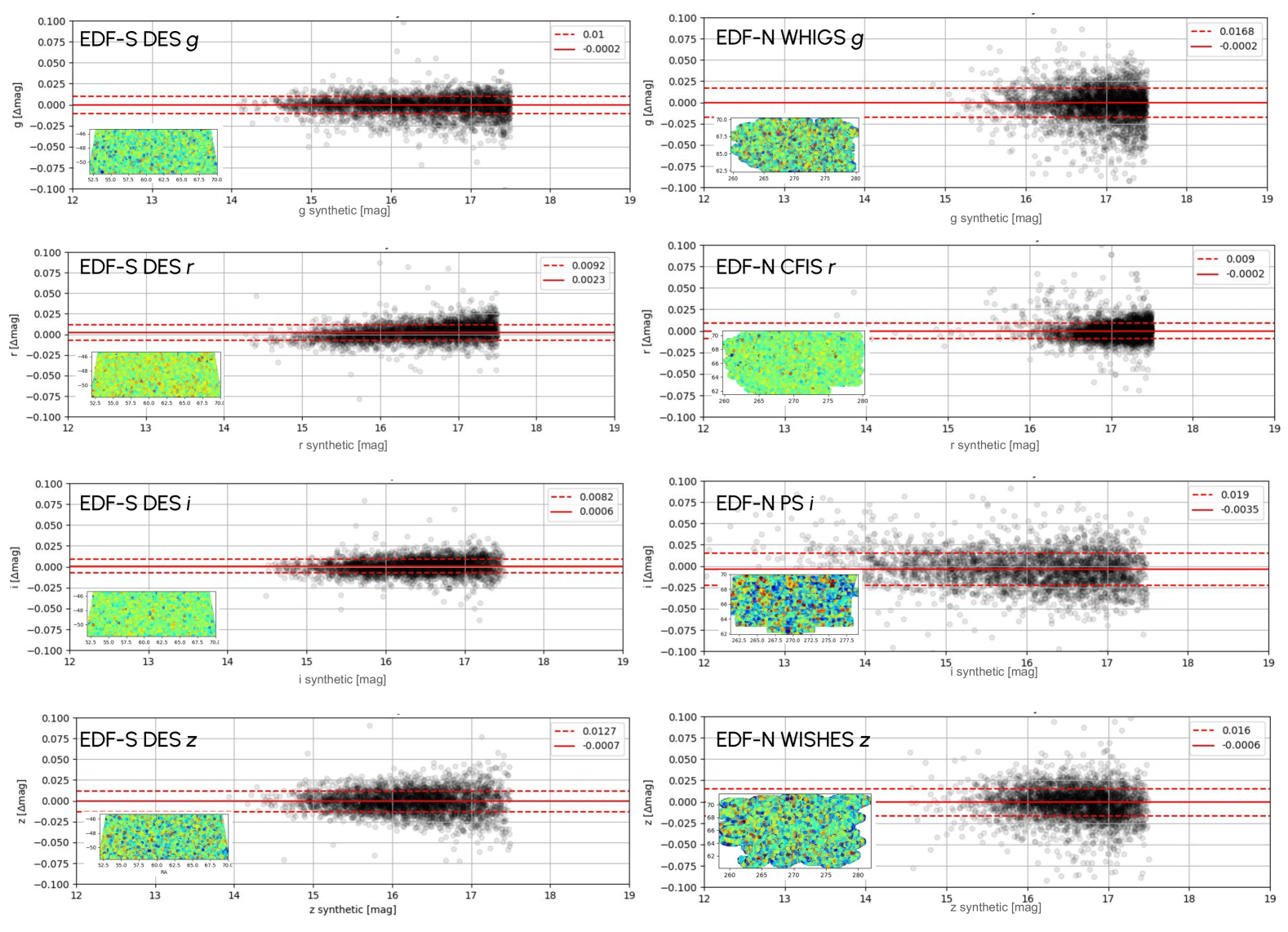
Figure 5: Photometric quality of the DES (left) and UNIONS (right) SEFs after calibration using Gaia spectrophotometry and the appropriate survey bandpass, assumed to be independent of focal plane location for Q1. Shown in each panel is the median offset (solid line) with respect to the Gaia calibrators, as well as the NMAD scatter (dashed line).

Figure 6: Per tile median magnitude residuals between the coadd PSF photometry and Gaia synthetic total magnitude for stars in the magnitude range 17–19. Top to bottom: EDF-N, EDF-S, and EDF-F. Left to right: $g$, $r$, $i$, and $z$ bands.

Figure 7: Intra-tile normalised NMAD scatter of the PSF fitting coadd photometry about the Gaia synthetic magnitudes for stars in the magnitude range 17–19. Top to bottom: EDF-N, EDF-S, and EDF-F. Left to right: $g$, $r$, $i$, and $z$ bands.

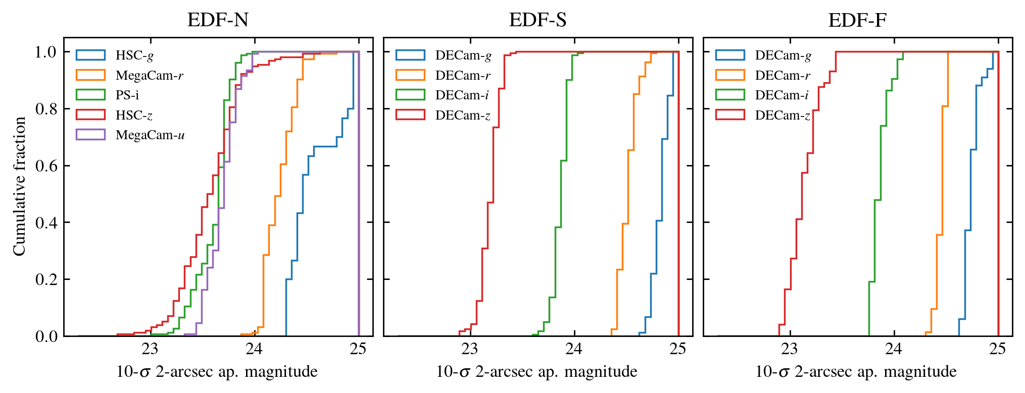
Figure 8: Cumulative fraction of the achieved depth per tile and band across the EDFs. Depth is defined as the 2″ diameter aperture magnitude for which the signal-to-noise ratio is 10.

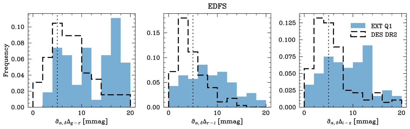
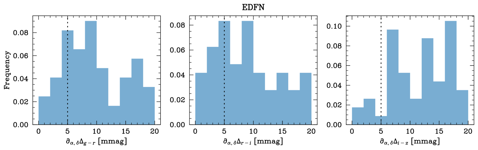
Figure 9: Colour offsets. Each panel here shows the spatial variation ($\partial_{\alpha,\delta}$) on scales of $0.\mathrm{°}3$ of the best-fit colour offset ($\Delta_{\rm color}$) for two of the EDFs. This statistic was determined for $g-r$ (left), $r-i$ (middle), and $i-z$ (right), relative to the average stellar colour distribution in the EDF-S area (top), and EDF-N (bottom). In the case of EDF-S we also show this result for DES DR2 data as the dashed dark histogram. The vertical black dotted line indicates the end-of-mission requirement.

On the other hand, the DES data (Abbott et al. 2018) and other Dark Energy Camera (DECam) (Flaugher et al. 2015) observations are processed and calibrated within the Euclid Collaboration using extended versions of pipelines originally developed for DES (Mohr et al. 2008, 2012; Desai et al. 2012) and extended for the CosmoDM data management system (Desai et al. 2015). These pipelines carry out detrending, astrometric calibration using SCAMP (Bertin 2006), position-dependent PSF modelling using PSFEx (Bertin 2011), and an initial photometric calibration using a statistical method that relies on the Gaia $G$, $BP$, and $RP$ photometry (George et al. 2020). In a final step, the DECam images are masked using a tool developed for Euclid (Desai et al. 2016), which employs PSF homogenisation (Darnell et al. 2009) in the creation of surface-brightness templates for each SEF.

The SEFs produced through the methods described above are then subjected to a homogeneous photometric calibration using the Gaia spectrophotometric data set and the corresponding survey passbands. For the Q1 calibration, these passbands are assumed to be constant across the different instrument focal planes. The Gaia data set (Gaia Collaboration: Prusti et al. 2016) offers a tremendous resource for producing stable, well-understood, ground-based photometry, because the Gaia photometry and spectroscopy are stable across the sky with a systematic uncertainty of around 2 mmag (Gaia Collaboration: Vallenari et al. 2023). As previously reported, photometric calibration of the Euclid SEF collection using the statistical transformations from Gaia $G$, $BP$, and $RP$ (George et al. 2020) to each of the external $griz$ bands demonstrated good consistency with the DES calibration, and improved photometric stability and internal consistency in comparison to the UNIONS calibration.

For the Q1 calibration, Gaia spectrophotometry is employed by using the survey passbands to create Gaia synthetic photometry for each of the Euclid external bands. Those calibrators are adopted for direct zero-point constraints and then combined with relative zero-point constraints from overlapping SEFs to solve for the SEF zero points and zero-point uncertainties within collections of SEFs that lie within overlapping patches of sky. The calibration tiles vary in size from 1–5 deg², depending on the density of SEFs in each of the EDFs.

Figure 5 shows – for a randomly selected sample of stellar sources – the scatter of the PSF-fitting stellar photometry versus the Gaia synthetic magnitude calibrators for EDF-S and EDF-N. The EDF-F data-set performance is similar to that for EDF-S. Each panel corresponds to a different band $griz$, and in the inset the median offset and normalised absolute median deviation (NMAD) scatter of the stellar PSF magnitudes are presented with respect to the calibrators. The inset sky maps plot the positional variation of the offsets and no spatial trends can be seen. In all cases, this photometric validation shows high quality and uniform SEF photometry. There are some differences from band to band in the NMAD scatter, which is reflective of the photometric flatness of the detrended SEFs and the quality of the derived zero points, which are impacted to some degree by the assumption that a single passband describes each survey band, independent of the location of the SEF within the focal plane of each instrument.

These homogeneously calibrated single-epoch images and their associated PSF models are processed into coadded images and per-object coadd-PSF models that are then used for photometry extraction alongside the VIS and NIR coadded images. The coaddition pipeline is a version of the coadd pipeline originally developed for the DES data management system (Mohr et al. 2008, 2012) and then later further developed within the CosmoDM data management system (Desai et al. 2015). The coadd pipeline uses a coadd tile definition to automatically select the relevant SEFs needed for coaddition, and then these images, their RMS noise maps and the metadata describing the zero point and world coordinate system (WCS) of each SEF are then coadded using calls to the SWarp code (Bertin et al. 2002; Bertin 2010). Similarly, RMS and flag maps are produced for each coadd image. This coadd pipeline has been applied to create high-quality, science ready, multi-band coadd imaging for a range of previous projects (e.g., Desai et al. 2012; Liu et al. 2015; Zenteno et al. 2016; Hennig et al. 2017).

The coadd-PSF modelling code has been created and validated as part of the Euclid development program. It draws upon the position-dependent PSF models extracted from every contributing SEF, scaling these models to have the measured flux and position appropriate for each SEF, and then assigning the appropriate RMS sky noise to each model. This collection of SEF-based PSF models are then coadded in the same manner as the SEF images themselves. These PSF models are created individually for every detected object, and they provide high-quality models of the resulting unresolved sources in the coadded images. PSF models for resolved objects are modelled under the assumption that the full flux of the source in each contributing SEF is assigned to the PSF model. A more complete description of this method along with validation tests will be presented in a future DR1 publication.

These coadd and PSF modelling codes have been integrated within the Euclid SGS software base for use in the external data processing. These data are validated using SourceXtractor++ to extract object catalogues from the images while using the prepared PSF models. The astrometry is cross-checked against Gaia, and the PSF-fitting magnitudes of unresolved (stellar) sources are compared to the synthetic magnitudes that have been extracted from the Gaia spectrophotometry.

To illustrate the photometric stability of the $griz$ coadd photometry in EDF-N (UNIONS: CFIS/MegaCam, HSC, PS), EDF-S, and EDF-F (DES/DECam), we show in Fig. 6 the median photometric offset between coadd PSF-fitting photometry and synthetic photometry computed from Gaia XP spectra. These figures show the relatively small tile-to-tile zero-point variations across most of each Q1 field, while also indicating that some tiles are outliers at the level of up to 0.04 mag from the photometric system of the calibrated SEFs used to create the coadds.

Figure 7 shows the normalised absolute deviation of the PSF magnitudes extracted from the coadds around the median offset described above. This measure serves as an indicator of the quality of the photometry of individual objects and can be compared to the NMAD scatter reported for the input SEFs presented in Fig. 5. In general, one would expect the photometric scatter in the coadds to always decrease relative to that seen in the input SEF population, but that is not the case for all tiles in the Q1 coadd data set. In addition, one can see that particular tiles have poorer performance than the others, suggesting imperfect performance of the coaddition and coadd PSF-modelling process. These metrics from the Q1 processing of the external data allowed us to identify and resolve these minor issues, which are being corrected in preparation for the Euclid DR1 processing.

Table 2: External data coadd and SEF data summary statistics. Photometry offsets and scatter are given in mmag, and scatter is estimated using NMAD.

Bandpasses	$g$	$r$	$i$	$z$
EDF-N
Median offset	$-1^{+9}_{-7}$	$-1^{+8}_{-4}$	$-19^{+4}_{-4}$	$\phantom{1}3^{+14}_{-8}$
Coadd scatter	$14^{+6}_{-3}$	$\phantom{-}9^{+3}_{-2}$	$\phantom{-1}8^{+1}_{-1}$	$12^{+9\phantom{0}}_{-3}$
SEF scatter	$17\phantom{{}^{+0}}$	$\phantom{-}9\phantom{{}^{+0}}$	$\phantom{-}19\phantom{{}^{+0}}$	$16\phantom{{}^{+00}}$
Depth	$25.3^{+0.3}_{-0.3}$	$24.3^{+0.2}_{-0.1}$	$23.7^{+0.1}_{-0.2}$	$23.6^{+0.2}_{-0.3}$
EDF-S
Median offset	$-1^{+6}_{-4}$	$-1^{+3}_{-3}$	$0^{+4}_{-4}$	1$-1^{+7}_{-8}$
Coadd scatter	$12^{+7}_{-3}$	$\phantom{-}7^{+2}_{-2}$	$7^{+3}_{-2}$	$\phantom{-}13^{+6}_{-4}$
SEF scatter	$10\phantom{{}^{+0}}$	$\phantom{-}9\phantom{{}^{+0}}$	$8\phantom{{}^{+0}}$	$\phantom{-}13\phantom{{}^{+0}}$
Depth	$23.9^{+1.2}_{-0.4}$	$24.0^{+1.2}_{-0.4}$	$23.9^{+1.3}_{-0.4}$	$24.1^{+1.1}_{-0.5}$
EDF-F
Median offset	$-1^{+4}_{-2}$	$-3^{+5}_{-5}$	$-2^{+5}_{-4}$	$-10^{+7}_{-7}$
Coadd scatter	$10^{+4}_{-4}$	$\phantom{-}6^{+5}_{-1}$	$\phantom{-}6^{+4}_{-2}$	$\phantom{-}10^{+5}_{-4}$
SEF scatter	$10\phantom{{}^{+0}}$	$\phantom{-}9\phantom{{}^{+0}}$	$\phantom{-}8\phantom{{}^{+0}}$	$\phantom{-}13\phantom{{}^{+0}}$
Depth	$24.1^{+1.1}_{-0.5}$	$23.9^{+1.2}_{-0.4}$	$23.9^{+0.6}_{-0.3}$	$23.9^{+1.3}_{-0.4}$

Table 2 contains summary statistics of the coadd and SEF photometry within each Q1 field. For EDF-N, EDF-S, and EDF-F, we find typical median offsets that are consistent with zero, with the exception of the PS data set. The NMAD scatter of the coadd photometry about the Gaia synthetic magnitudes is approximately 1%, and the depths are consistent with the depth requirements set by the Euclid mission. The photometric scatter within the SEFs is smaller in DES than in UNIONS, and in most cases the photometric scatter in the coadds is smaller, as expected. Figure 8 shows the depth distributions of each band within each of the Q1 fields. These depths are summarised in Table 2.

To assess the colour stability of the Q1 data set, we utilize the stellar locus (SL). We compute a fiducial SL for EDF-N and EDF-S and assume that intrinsic variations (for example, due to the spatial variations of the underlying stellar populations in the Galaxy) on the SL are minimal in these areas. We run the SL analysis in EDF-N and EDF-S. In the former case, we use the bands HSC $g$, MegaCam $r$, PS $i$, and HSC $z$, and in the latter DECam $g$, $r$, $i$, and $z$. The fiducial SL is built using high-confidence non-saturated stars with low photometric uncertainties. The magnitudes and colours adopted are measured using SourceXtractor++ on the coadd images as part of Euclid’s internal validation pipeline. For the purpose of this colour validation test we must first remove the variations due to Galactic extinction. Therefore, all magnitudes are extinction corrected using Schlegel et al. (1998) dust maps, with Schlafly & Finkbeiner (2011) corrections and adopting the Cardelli et al. (1989) extinction law.

Given a list of excellent photometric quality objects, we build the SL model by fitting a Gaussian mixture model, taking into account all the photometric uncertainties. To avoid overfitting, this model was tuned to represent the data set with the least amount of components. We then partition the sky into $0.\mathrm{°}3$ bins, each containing at least 200 stars. For each bin, we measure a colour offset that maximizes the likelihood of its stars being drawn from the fiducial SL model. The likelihood maximisation is done through a Nelder–Mead gradient descent method. This effectively produces a map of best-fit colour offsets.

To assess the stability of the colour in the Q1 EXT data we need to take the spatial derivative of the colour offset maps described above. In Fig. 9 we show this quantity for EDF-S and EDF-N. In the case of EDF-S we also compare it to what is obtained using public DES DR2 data (Abbott et al. 2021). On all panels the dotted vertical line marks the end-of-mission requirement of 5 mmag.

We note that the colour stability for the Q1 data set is generally below the end-of-mission requirements. One can see in the upper panels of Fig. 9 that the DES DR2 colour stability is better, but it also does not meet the Euclid requirements. The Q1 data quality is affected by a combination of factors that mostly have affected the integrated version of the PSF-modelling code and have since been identified and corrected. With these code fixes, the incidence of tiles with strongly outlying photometry has been reduced, but has not been completely resolved. Further work to improve the integrated versions of the coadd and PSF modelling software is ongoing in preparation for the Euclid DR1 processing.

6 Photometric masks

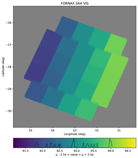
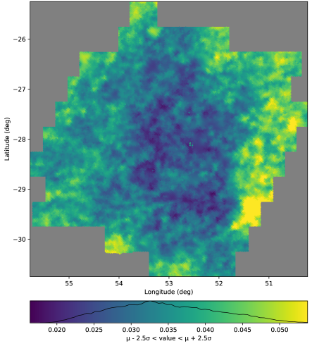
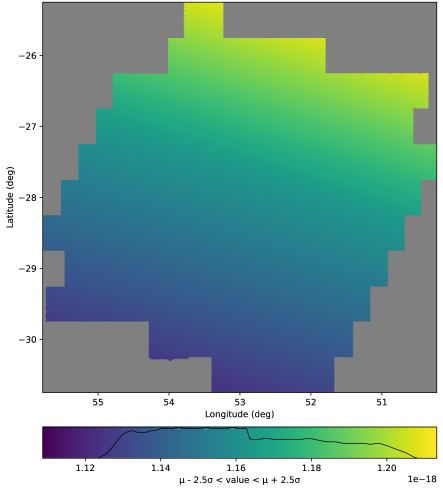
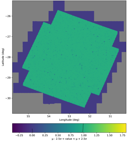
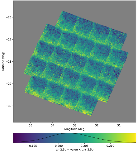
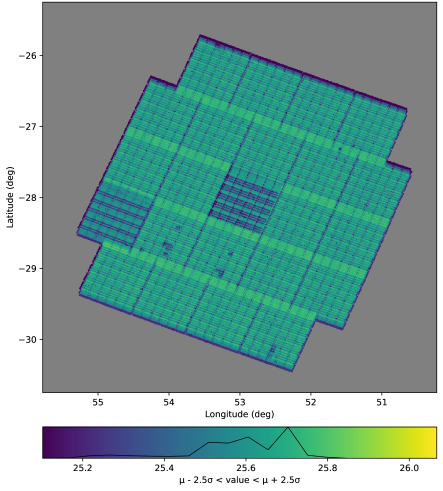
Figure 10: Examples of photometric masks for the EDF-F field. Top: SAA and VIS Galactic extinction and zodiacal light masks. Bottom: VIS coverage, PSF, and depth masks. Histograms of the represented signals are shown within the colour bars.

A set of masks allowing for the assessment of the data quality over each of the Q1 EDFs were produced by the VMPZ-ID PF. While this PF is formally a Level 3 (LE3) PF in the SGS, it is at the interface between LE2, where data are at the pixel level, and LE3 that consider the whole Euclid mission data set on the celestial sphere. The information from the VIS, NIR, EXT, and MER masks at the exposure and tile level is combined into a series of masks in the HEALPix (Górski et al. 2005) format using a $N_{\mathrm{side}}=16\,384$, which corresponds to a resolution of approximately $12.\mathrm{″}88$. VMPZ-ID also produce so–called DpdHealpixInfoMapVMPZ that enable us to track satellite and instrumental properties and project them on the sky, allowing for easy cross-check between spatial information (for example the depth at a given point of the survey) with temporal information (for example the value of a temperature sensor on the Euclid focal plane) and look for possible effects affecting the performance of the Euclid mission. The masks distributed with the Q1 data release are listed in Table 3.

Table 3: Summary of the main characteristics of the photometric maps. For each mask we give the mask family (indicating if it is related to the survey properties, to the satellite status, to the instrument performance, or to the sky emission), the mask type as defined in the text, the InfoMap type (only for InfoMap masks) and the numerical type. We also indicate if masks per band are produced.

Mask	Mask family	Mask product type	InfoMap type	Numerical	Per-band	Comments
			type	type	mask
Tile index	Survey	DpdHealpixInfoMapVMPZ	Tile	integer	no
Solar aspect angle	Survey/Satellite	DpdHealpixInfoMapVMPZ	SAA	float32	no
Alpha angle	Survey/Satellite	DpdHealpixInfoMapVMPZ	AA	float32	no
Beta angle	Survey/Satellite	DpdHealpixInfoMapVMPZ	BA	float32	no
Exposure time	Survey	DpdHealpixInfoMapVMPZ	Exposures	float32	yes	Euclid only
Footprint	Survey/Instrument	DpdHealpixFootprintMaskVMPZ	…	float32	no	all bands combined
Coverage	Survey/Instrument	DpdHealpixCoverageMaskVMPZ	…	float32	yes
Bit mask	Instrument	DpdHealpixBitMaskVMPZ	…	uint32	yes
Depth	Instrument	DpdHealpixDepthMapVMPZ	…	float32	yes
RMS Noise	Instrument	DpdHealpixInfoMapVMPZ	Noise	float32	yes
Point-spread function	Instrument	DpdHealpixInfoMapVMPZ	PSF	float32	yes
Zodiacal light	Sky emission	DpdHealpixInfoMapVMPZ	ZodiacalLight	float32	yes	Euclid only
Galactic extinction	Instrument	DpdHealpixInfoMapVMPZ	GalacticExtinction	float32	yes	Euclid only

In terms of Euclid data products the photometric masks are constructed per MER data products (Euclid Collaboration: Kang et al., in prep.) and are of five main types.
– DpdHealpixFootprintMaskVMPZ mask has value 1 if the sky region has been observed and 0 otherwise in any band (Euclid and EXT).
– DpdHealpixCoverageVMPZ has values between 0 and 1, representing the coverage for the pixel each of the Euclid and EXT bands.
- DpdHealpixBitMaskVMPZ is an unsigned integer mask with its bits associated with the MER flags.
– DpdHealpixDepthMapVMPZ is a float map representing the depth as computed from the RMS for each Euclid and EXT band.
– DpdHealpixInfoMapVMPZ is a generic mask to represent different quantities of interest.

In practice, 108 photometric masks per MER tile have been produced for the Q1 data release. In Table 3 we summarise the main properties of those masks. A more detailed description of each of the masks is given below. Examples of those masks for the EDF-F region are shown in Fig. 10.

6.1 Survey-definition masks

– Tile number: This mask, of type DpdHealpixInfoMapVMPZ, is constructed so that for each HEALPix pixel the number of the MER tile on which it lies is stored in integer form.
– Footprint: A footprint mask defining the observed or valid sky area is stored in the form of a DpdHealpixFootprintMaskVMPZ. It is constructed per Euclid and EXT bands. Starting from the MerBksMosaic maps we set the sky regions observed in all bands to one and the others to zero. MER tile pixels for which the RMS is zero or larger than a given threshold are considered as not observed. All MER tile pixels within a HEALPix pixel are combined using a logical and operator.
– Coverage: The coverage per band (Euclid and EXT) is calculated from the MER background-subtracted mosaic (hereafter MerBksMosaic maps. The footprint MER tile pixels, for which the RMS value is zero or larger than a given threshold, are considered as not observed. Furthermore, for the Euclid bands polygon masks are used to exclude sky regions affected by bright star emission. For each HEALPix pixel, the coverage is given by the fraction of valid MER tile pixels.

6.2 Satellite related masks

– Satellite orientation angles: for each HEALPix pixel the average SAA, azimuth or $\alpha$ angle (AA), and beta angle (BA) in degrees (see Euclid Collaboration: Scaramella et al. 2022) are calculated from the MER Layering files. They are stored in the form of a DpdHealpixInfoMapVMPZ.
– Exposure Time: for each of the Euclid bands the average exposure time per HEALPix pixel is calculated and stored as a DpdHealpixInfoMapVMPZ.

6.3 Instrumental properties masks

For each of the Euclid and EXT bands, we obtain masks of the main instrumental properties from the MerBksMosaic maps. For each HEALPix pixel, the weighted average of the instrumental properties is computed. We assign zero weight to MER tile pixels with RMS equal to zero or above a given threshold.
– RMS noise: DpdHealpixInfoMapVMPZ that monitors the average RMS noise in the MerBksMosaic maps.
– Depth: DpdHealpixDepthMapVMPZ that monitors the depth obtained from the RMS moise:

$$m=-2.5\log 10\left(\mathrm{RMS}\cdot d_{\mathrm{th}}\cdot\sqrt{\frac{A_{\mathrm{aper}}}{A_{\mathrm{pixel}}}}\,\right)+\textrm{ZP},$$ (1)

with ZP the zero point as found in the MerBksMosaic maps. The detection threshold, $d_{\mathrm{th}}$, is fixed to 5 corresponding to a 5$\,\sigma$ detection. $A_{\mathrm{aper}}$ and and $A_{\mathrm{pixel}}$ represent the detection aperture and pixel areas, respectively. For the Q1 data release we have chosen a 2$\arcsec$ diameter aperture to compute the depth.
– PSF: DpdHealpixInfoMapVMPZ that monitors the FWHM of the PSF. Because the full width at half maximum (FWHM) can be measured only on bright stars, 2D interpolation is performed across the tile area.
– Bit Mask: DpdHealpixBitMaskVMPZ obtained from a bit-by-bit bitwise or of the Bit Mask of the MerBksMosaic maps.

6.4 Sky emission masks

Following Euclid Collaboration: Scaramella et al. (2022) we construct per-tile masks of the zodiacal light emission and Galactic extinction at the Euclid bands. These masks are stored as DpdHealpixInfoMapVMPZ.

7 Data access

The public Euclid science archive at the ESAC Science Data Centre (ESDC) opened on 19 March 2025 offering the curated Q1 data products at the following address: https://eas.esac.esa.int/sas/. Information about the Q1 data release is presented at https://www.cosmos.esa.int/en/web/euclid/euclid-q1-data-release.

The MER mosaics in the four Euclid bands and four EXT bands, as well as VIS/NIR calibrated frames (and their auxiliary data sets) can be searched and downloaded from the web interface. An image cutout service on the mosaics is also offered. All MER, PHZ, and SPE catalogues are ingested into the database and can be queried, through the IVOA Table Access Protocol, with Astronomical Data Query Language (ADQL), for which tutorials are provided. The results of queries can be downloaded or overlaid on the different Hierarchical Progressive Survey (HiPS) maps. Spectra can also be queried and retrieved using the IVOA DataLink protocol. A subset of the data set can be accessed through ESASky at https://sky.esa.int/.

Data can also be accessed through Python with the Euclid astroquery toolkit to query catalogues or retrieve files (Ginsburg et al. 2019). However, since the FITS files are very large, we promote the use of the ESA Datalabs science platform (Navarro et al. 2024), accessible at https://datalabs.esa.int/. Access to Datalabs is limited to users with an ESA Cosmos account, which can be obtained through self-registration with invitation code ‘EUCLIDQ1’. This provides direct access to the Euclid Q1 data repository with tutorial Jupyter notebooks to access, visualise, manipulate, and analyse data.

As explained in Sect. 4.4, the complementary background-preserving stacks of the dark cloud will be fully curated soon. Their location and access will be communicated on the Euclid consortium’s website at https://www.euclid-ec.org.

8 Scientific exploitation of the Q1 data

The very large range of non-cosmological science enabled by Euclid is evidenced by already $\sim$ 30 papers submitted as an initial batch of results at the time of Q1. They range from nearby galaxies to strong lenses and quasars, including the detection of rare objects. The publications also place a strong emphasis on automated and scalable search and modelling methods, in preparation for efficient exploitation of the vast amount of Euclid data to come in DR1 to DR3.

8.1 Nearby galaxies

Marleau et al. (2025) takes advantage of the unprecedented depth, spatial resolution, and field of view of Q1 data to detect and characterise dwarf galaxies. We have identified 2674 candidates, corresponding to 188 dwarfs per deg², in a 14.25 deg² area of EDF-N. Candidates were selected using a semi-automatic method based on Euclid pipeline measurements, followed by cuts in surface brightness, magnitude, morphology, and $I_{\scriptscriptstyle\rm E}-H_{\scriptscriptstyle\rm E}$ colour. A final visual classification assigned morphology, number of nuclei, globular cluster richness, and blue compact centres.

8.2 Galaxy morphology

Q1 data are used as a vast training data set for ‘foundation’ deep-learning models. The goal is to produce catalogues of galaxy properties, in particular morphology-related features.

Euclid Collaboration: Walmsley et al. (2025b) presents a detailed visual morphology catalogue created by fine-tuning the Zoobot foundation deep-learning model on annotations from an intensive 1-month campaign by Galaxy Zoo (Lintott et al. 2008) volunteers. Placing a trained deep-learning model within the survey image processing pipeline allows immediate morphology measurements, producing a detailed visual morphology catalogue for Q1 in weeks instead of years. Detailed visual morphology refers to the recognisable features that comprise a galaxy, such as bars, spiral arms, and tidal tails. Our catalogue includes such galaxy features for the 378 000 bright ($I_{\scriptscriptstyle\rm E}<20.5$) or extended (area ${\geq}$ 700 pixels) galaxies in Q1. This catalogue is the first 0.4% of the approximately 100 million galaxies where Euclid will ultimately resolve detailed morphology. Our measurements have already proven useful for exploring the relative abundance of stellar bars in disc galaxies from $z=1$ to 0 in Euclid Collaboration: Huertas-Company et al. (2025). Stellar bars are key structures in disc galaxies, driving angular momentum redistribution and influencing processes such as bulge growth and star formation. Therefore, tracing their abundance over time serves as a proxy for disc assembly. We identified 7711 barred galaxies, which is an order of magnitude more than previous HST and James Webb Space Telescope (JWST) based results. At fixed redshift, massive galaxies exhibit higher bar fractions, while lower-mass systems show a steeper decline with redshift, suggesting earlier disc assembly in massive galaxies.

Euclid Collaboration: Siudek et al. (2025) presents the first application of AstroPT, a multi-modal autoregressive foundation model, to Euclid’s Q1 data release. Trained on around 300 000 optical and infrared images along with SEDs, AstroPT enables efficient self-supervised learning for key astrophysical tasks. We demonstrate its effectiveness in galaxy-morphology classification, redshift estimation, similarity searches, and anomaly detection. These findings showcase the potential of foundation models for scalable, data-driven astrophysical analysis in future larger Euclid data releases.

Euclid Collaboration: Quilley et al. (2025) also characterises the morphology of Q1 galaxies, but uses more conventional Sérsic profiles. Euclid’s exquisite image resolution and the large survey area of Q1 data release enable a robust morphological description for more than a million galaxies. The analysis confirms the bimodality of galaxy populations between late- and early-type galaxies, which reflects further differences in their physical properties.

8.3 Star-forming galaxies

Euclid Collaboration: Enia et al. (2025) provides a first view of the star-forming main sequence (SFMS) in the EDFs. The SFMS is a fundamental relation linking together the galaxies’ budget of cold gas, the efficiency in converting it into stars, and its stellar content. It manifests itself as a tight relation between galaxy stellar masses and star-formation rates across different epochs. We investigated the SFMS in the redshift range $0.2<z<3.0$ and recovered more than 30 000 galaxies with $\log_{10}(M_{*}/M_{\odot})>11$, giving a precise constraint of the SFMS at the high-mass end. These results highlight the potential of Euclid in studying the fundamental scaling relations that regulate galaxy formation and evolution.

At higher redshifts $z>3$, our understanding of cosmic star formation mostly relies on rest-frame UV observations. However, these observations overlook massive, dust-obscured sources, and indeed recently infrared data from the Spitzer Space Telescope and JWST have revealed a hidden population at $z\simeq 3$–6 with extreme red colours. Taking advantage of the overlap between imaging in the EDFs and ancillary Spitzer Space Telescope observations, Euclid Collaboration: Girardi et al. (2025) identified 3900 extremely red objects with $H_{\scriptscriptstyle\rm E}-\textrm{IRAC2}>2.25$, dubbed HST-to-IRAC extremely red objects. Our results confirm that HIERO galaxies may populate the high-mass end of the stellar mass function at $z>3$, with some sources reaching extreme stellar masses $(M_{*}>10^{11}M_{\odot})$ and exhibiting high dust attenuation values $(A_{V}>3)$, contributing to a more complete census of early star-forming galaxies. Given the extreme nature of this population, characterising these sources is crucial for building a comprehensive picture of galaxy evolution and stellar mass assembly across most of the history of the Universe. This work demonstrates Euclid s potential to provide statistical samples of rare objects.

The first years of observations with JWST have revealed a novel population of compact red sources, the so-called little red dots. They are characterised by a peculiar v-shaped SED, namely a blue rest-frame UV continuum and a red rest-frame optical continuum, and were mainly observed at $z>4$. The nature of these LRDs is debated, their emission being consistent with either hosting an active galactic nuclei (AGN) or emission from dusty star formation. In Euclid Collaboration: Bisigello et al. (2025) these sources are identified by combining a slope selection, a criterion for compactness and visual inspection. We found over $3000$ LRD candidates at $z<4$, while previous JWST results mostly found objects at higher redshifts. We also show that LRDs are not the dominant AGN population in this redshift range.

8.4 Passive galaxies and galaxy quenching

Galaxy quenching is the sudden cessation of star formation in galaxies. Investigating the drivers of the quenching of star formation in galaxies is key to understanding their evolution. Using Q1 data, Euclid Collaboration: Corcho-Caballero et al. (2025) develops a probabilistic classification framework, that combines the average specific star-formation rate inferred over two timescales ($10^{8}$ and $10^{9}$ years), to categorise galaxies as ‘Ageing’ (secularly evolving), ‘Quenched’ (recently halted star formation), or ‘Retired’ (dominated by old stars). At $z<0.1$ and $M_{*}\geq 3\,\times\,10^{8}M_{\odot}$, we obtain fractions of 68–72%, 8–17%, and 14–19% for Ageing, Quenched, and Retired populations, respectively, consistent with previous studies. We also explore how these fractions vary with different factors, including redshift, stellar mass, morphology, and chemical composition, finding, for example, that Ageing and Retired galaxies dominate at the low and high-mass ends, respectively, while Quenched galaxies surpass the Retired fraction for $M_{*}\leq 3\,\times\,10^{10}M_{\odot}$. Additionally, the evolution with redshift shows increasing/decreasing fraction of Ageing/Retired galaxies and Ageing galaxies generally exhibit disc morphologies and low metallicities.

8.5 AGN evolution

Several papers have used Q1 data to explore AGN science. In Euclid Collaboration: Matamoro Zatarain et al. (2025), three multi-wavelength catalogues of AGN candidates from the Q1 EDFs are introduced. Traditional photometric selections, involving optical, NIR, mid-IR, and spectroscopic diagnostics are employed to analyse the AGN populations using Euclid data. Additionally, we explore new colour-colour criteria to identify AGN. This catalogue of AGN candidates is complemented by identification of X-ray AGN in the Q1 footprint in Euclid Collaboration: Roster et al. (2025). Here, the most likely X-ray emitters among the Euclid sources are first identified and then, using machine learning, X-ray objects are classified as Galactic or extragalactic. Finally, for the extragalactic sources, photometric redshifts, their luminosity, and their basic SED properties are presented.

This multiwavelength AGN candidate catalogue is then used to understand the performance of new machine-learning methods presented in Euclid Collaboration: Stevens et al. (2025) and Euclid Collaboration: Margalef-Bentabol et al. (2025). The first paper explores a novel application of diffusion-based inpainting for the identification of AGN using VIS images alone. By exploiting the reconstruction error in regenerated galaxy cores, this method achieves high recall rates with candidates from the traditional multi-wavelength methods presented in Euclid Collaboration: Matamoro Zatarain et al. (2025) and Euclid Collaboration: Roster et al. (2025). Using only VIS images for training and inference, no prior knowledge about the presence of an AGN component is required, making it applicable for use with future Euclid data releases. The second paper (Euclid Collaboration: Margalef-Bentabol et al. 2025) presents a deep learning-based method to identify and quantify AGN in Euclid galaxy images by estimating the central point source contribution. Trained on ‘Euclidised’ mock images with injected AGN, the model accurately recovers the AGN contribution fraction. Applied to Euclid data, 8% of galaxies show an AGN contribution fraction above 20%. We also find that AGN luminosity correlates with host galaxy mass, suggesting faster supermassive black hole (SMBH) growth in massive galaxies. AGN are more common in quiescent galaxies and most luminous in massive and starburst systems, supporting a link between SMBHs and galaxy assembly.

The machine-learning approach is further explored in Euclid Collaboration: La Marca et al. (2025) to study the role of major mergers in triggering AGN using a classical binary classification of galaxies into ‘active’ and ‘non-active’. The paper also examines AGN properties, such as the point-source contribution, as well as luminosity, with four different AGN-selection techniques explored. The main results are that mergers influence all types of AGN candidates, but overall they do not seem to be the main triggering mechanism. However, major mergers become more and more important in the fuelling of the most luminous AGN, indicating that they might be the dominant triggering mechanism of the most powerful AGN in the Universe.

Q1 data also allowed us to explore the dust-obscured red quasi-stellar objects. In Euclid Collaboration: Tarsitano et al. (2025) a selection method based on machine-learning and multidimensional colour analysis is developed, identifying over 150 000 candidate red QSOs. Compared to VISTA+DECAm-based colour selection criteria, Euclid’s superior depth, resolution, and optical-to-NIR coverage improves the identification of the reddest, most obscured sources. To refine the selection function, probabilistic random-forest classification is combined with uniform manifold approximation and projection (UMAP) visualisation, achieving 98% completeness and 88% purity. This work provides a first census of candidate red QSOs in Q1 and sets the groundwork for future data releases, including spectral and host morphology analyses.

8.6 Cosmic environment

The impact of the environment in the properties of galaxies and galaxy clusters is addressed in several papers. Euclid Collaboration: Cleland et al. (2025) studies how the local environment of a galaxy affects its evolution. To do this, we measure the local environmental density for each galaxy in the Q1 sample. We then calculate the fractions of passive galaxies and early-type galaxies as function of stellar mass, environment, and redshift. We find that, up to $z\simeq 0.7$, the environment plays a significant role in transforming galaxies from star-forming to passive. At $z>0.7$, the passive fraction and early-type-galaxy fraction are mostly determined by the stellar mass, and as such the environment only has a weak effect on these properties.

Galaxy morphologies and shape orientations are also expected to correlate with their large-scale environment, as they grow by accreting matter from the cosmic web and are subject to interactions with other galaxies. Euclid Collaboration: Laigle et al. (2025) extracts cosmic filaments from the Q1 data at $0.5<z<0.9$, and analyses the 2D alignment of galaxy shapes with large-scale filaments as a function of Sérsic indices and masses. We confirm the known trend that more massive galaxies are closer to filament spines. At fixed masses, morphologies correlate with both density and distances to large-scale filaments. In addition, the large volume of this data set allows us to detect a signal indicating that there is a preferential alignment of the major axis of massive early-type galaxies along cosmic filaments.

Clusters are also shaped by their connection to the cosmic web. In particular, since they are nodes in the large-scale cosmic web, a relevant property is the number of filaments connected to a cluster, known as its ‘connectivity’. Euclid Collaboration: Gouin et al. (2025) uses Q1 data to investigate the connectivity of galaxy clusters and how it correlates with their own and their galaxy-member properties. Around 220 clusters in the redshift range $0.2<z<0.7$ were analysed. In agreement with previous measurements, we find that the most massive clusters are, on average, connected to a larger number of cosmic filaments, which is consistent with hierarchical structure formation models. We also explored possible correlations between connectivity and the fraction of early-type galaxies and the Sérsic index of galaxy members. Our result suggests that the clusters populated by early-type galaxies exhibit higher connectivity compared to clusters dominated by late-type galaxies.

8.7 Strong gravitational lensing

The combination of a wide field of view with the capability of resolving small Einstein radii makes Euclid the most efficient instrument for finding strong lenses ever built. Most galaxy-scale strong lenses are expected to have Einstein radii smaller than $1.\mathrm{″}0$, below the resolution limits of ground-based surveys, while Euclid’s space-based PSF can resolve lenses down to an Einstein radii of around $0.\mathrm{″}6$ in large numbers. Euclid Collaboration: Walmsley et al. (2025a) presents the ‘strong lensing discovery engine’, which combines the strengths of AI, citizen scientists, and experts into a system that efficiently searches for strong lenses in Euclid data. In particular, the lenses are found through an initial sweep by deep-learning models, followed by Space Warps citizen-science inspection, expert vetting, and detailed lens modelling. A catalogue of 497 galaxy-galaxy strong lenses was constructed from Q1 data, which already doubles the total number of known lens candidates with space-based imaging. Extrapolating to the complete EWS implies a likely yield of over 100 000 high-confidence candidates, transforming strong lensing science.

The Q1 search with the strong-lensing discovery engine is detailed in a series of four additional papers. Euclid Collaboration: Rojas et al. (2025) uses Q1 images containing galaxies with high velocity dispersion, spectroscopically identified in the Sloan Digital Sky Survey (SDSS) and the Dark Energy Spectroscopic Instrument experiment (DESI), to search for lenses and build an initial training set for our machine-learning models. Euclid Collaboration: Lines et al. (2025) analyses five machine learning models and compares their performance on real Euclid images. Euclid Collaboration: Li et al. (2025) reports the discovery of four new double-source-plane lenses in Q1. Strong gravitational lensing systems with multiple source planes are powerful tools for probing the density profiles and dark matter substructure of the galaxies, and the ratio of Einstein radii is related to the dark energy equation of state. DSPLs are extremely rare, but Euclid is expected to discover over 1000 such systems. Finally, Euclid Collaboration: Holloway et al. (2025) discusses lessons learned for future Euclid data releases, presenting a Bayesian ensemble method that combines lens classifiers to further optimise lens discovery within our discovery engine for DR1.

In addition to searching methods, also modelling techniques need to be optimised for handling Euclid’s vast data set. Euclid Collaboration: Busillo et al. (2025) presents a Bayesian neural network, dubbed LEns MOdelling with Neural networks (LEMON) designed to model Euclid’s gravitational lenses efficiently. LEMON estimates key parameters of the mass and light profiles and is shown to perform well on simulated Euclid lenses, real Euclidised HST lenses, and real Q1 lenses.

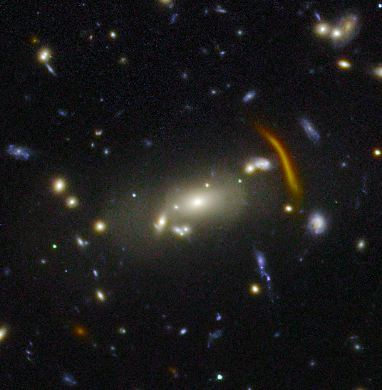
Figure 11: The strong-lensing cluster Abell 2280 in the EDF-N Q1 area. This image is at the full VIS resolution, $$$\times$$$ wide, using VIS and all NISP photometric images for colour information.

8.8 Galaxy clusters

The algorithms developed and implemented in the SGS LE3 pipeline for cluster detection have already being run on the Q1 data (Euclid Collaboration: Bhargava et al., in prep.). They found several hundred high-confidence clusters in the Q1 area, stretching across in the redshift range $0.2<z<1.5$, validating the pipelines ahead of DR1 and allowing for improvements.

Also using Q1 data, Euclid Collaboration: Bergamini et al. (2025) constructs the first catalogue of strong lensing galaxy clusters observed by Euclid, based on the visual inspection of over a thousand richness-selected known galaxy clusters. Most of these galaxy clusters had never been observed from space before (such as Abell 2280, Fig. 11), and only a few were previously known to host strong lensing features. Specifically, we identified 83 strong gravitational lenses, including 14 exhibiting secure strong lensing features such as tangential and radial arcs and multiple images. These galaxy clusters will be re-observed by Euclid multiple times during the mission as part of the EDS. Based on the number density of detected lensing galaxy clusters, we expect that Euclid will observe more than 6000 strong lensing galaxy clusters in its wide survey. This estimate is consistent with the forecasts from simulations in the $\Lambda$CDM cosmological model. Our work demonstrates the huge potential of the Euclid mission for discovering new strong lensing galaxy clusters.

Euclid Collaboration: Mai et al. (2025) deals with the detection of galaxy clusters and protoclusters at high redshift $(z>1.3)$. Euclid is expected to detect tens of thousands of such objects over the course of its mission, and Q1 is large enough to detect tens of clusters and hundreds of protoclusters at these early epochs. To extend the detection to this redshift range, we have combined Euclid and Spitzer Space Telescope observations of the Q1 EDFs. We compute local projected densities of Spitzer-selected galaxies with two methods, and use high values of the computed surface density as signposts for cluster and protocluster candidates. We found that 2–3% of the surface densities measured in EDF-N and EDF-F are $3\,\sigma$ above the mean density. This is a clear indication that a large part of the less massive galaxies in these two EDFs have larger densities than galaxies with the same mass in the field, and hence there is high potential that they belong to groups or clusters.

8.9 Transients

While Q1, in distinction to future data releases, does not include multiple epoch observations of the target fields, Duffy et al. (2025) reports on serendipitous Euclid observations of previously known transients reported to the Transient Name Server in the EDFs. We were able to make photometric measurements at the location of 161 transients, obtaining deep photometry or upper limits in $I_{\scriptscriptstyle\rm E}$, $Y_{\scriptscriptstyle\rm E}$, $J_{\scriptscriptstyle\rm E}$, and $H_{\scriptscriptstyle\rm E}$ at various phases of the transient light-curves. These observations include one of the earliest NIR detection of a Type Ia supernova, 15 days prior to peak brightness and the late-phase (435.9 days post peak) observations of the core-collapse supernova 2023aew. In addition to this the hosts galaxies of several transients were detected that previously had been classified as hostless.

9 Caveats

Q1 is the first release of Euclid data by the SGS in a sequence ultimately gearing up towards DR3 in the early 2030s. The data processing is not yet fully mature, and many of the processing functions have identified pathways towards improvements, some that will be implemented for DR1 and some whose development will be longer and appear in subsequent data releases. We take the opportunity to remind the users of Q1 data of a few important caveats to keep in mind when working with the data.

One important caveat discussed in Euclid Collaboration: Le Brun et al. (2025) is to be careful when using redshifts from the catalogues. On the one hand, by design, the SGS pipelines produce one spectrum for each source of the MER catalogue with $H_{\scriptscriptstyle\rm E}<22.5$. This corresponds to about 4.3 million spectra. On the other hand, the expected number of sources with H$\alpha$ flux above the nominal flux limit of the EWS (predicted from luminosity functions for an area of 63.1 deg²) is of the order of 100 000. This corresponds to about 2.5% of the spectra. These data also include further spectra for stars and galaxies/AGN outside of the target redshift range, measured from other lines. These will still be a small part of the total, so that the fraction of spectra allowing for the measurement of a redshift is below 10%. Yet, the SGS pipeline provides a redshift estimate for everyone of them. The challenge the SGS is confronted with is to correctly assess the reliability of the automated redshift measurements. The issue will be even more complex for DR1 when attempting to increase the limiting magnitude of the extracted sample. Meanwhile, we recommend to work with the highest quality of spectra, and to check if possible the redshift by examining the 1D spectra of the sources of interest. This can only be done for small samples of sources.

Another caveat concerns the imaging data. The SGS pipeline is optimised for the Euclid mission core science goals, namely to measure the shape and photometry of galaxies at redshifts above $z=0.5$, that is for objects with arcsecond size on the sky. While the VIS and NIR PFs do strive to preserve low surface brightness features as much as possible, these are mostly filtered out at the MER stage when the stacks are being built. Members of the Euclid Consortium working on the intracluster medium, on local galaxies, or on Galactic cirrus are devising alternative processing outputs derived from the VIS and NIR calibrated frames. These alternatives will become available in the future through the Euclid Datalabs interface discussed in Sect. 7, but not in time for Q1. We additionally caution users about the MER catalogue from the LDN 1641 region, as the structure of this field is very different from typical EWS fields for which the SGS PFs are optimised, and advise them to start their analysis from the VIS and NIR LE2 calibrated frames for this part of the data set.

Finally, we note that many PFs have issued release notes for their processing procedures, either in the papers submitted with Q1, or in the explanatory supplement published online from the release page at https://www.cosmos.esa.int/en/web/euclid/euclid-q1-data-release. We recommend all users of the Q1 data to read these descriptions carefully.

10 Conclusions

Q1 contains data from about 7 days of Euclid observations. Over these 63 deg² of the EWS Euclid already detects about 30 million sources, including galaxies, stars, quasars, brown dwarfs, and even solar system objects. This release is only the first part of Euclid’s survey data, meant as an initial batch of data for scientific use, but also to provide to the community an impression of what is to come: in the sense of types of data and data quality, to sharpen tools and define interesting science questions, but also to sensitise the community to the sheer size of the Euclid surveys. The first ‘cosmological’ data release (DR1), likely to be in late 2026, will cover 30 times the Q1 area or about $1900\,\textrm{deg}^{2}$, and hence about 1.5 orders of magnitude more objects in every category. Any science project that finds a handful objects of interest in Q1 will find hundreds in DR1; however, an easy project in Q1 involving human eyes as part of the analysis or classification cascade might become challenging in DR1, and any analysis tasks that due to sheer catalogue size are already hard in Q1 will require very different tools in DR1 to be feasible.

The first wave of scientific publications based on Q1, sketched in Sect. 8, illustrates the growing role that machine learning will play in the analysis of upcoming big data sets in astronomy – including Euclid. Approximately half of the scientific papers accompanying Q1 make use of ‘artificial intelligence’: generative and classification models are used for finding and characterising AGN in galaxies (Euclid Collaboration: Stevens et al. 2025; Euclid Collaboration: La Marca et al. 2025; Euclid Collaboration: Margalef-Bentabol et al. 2025; Euclid Collaboration: Roster et al. 2025; Euclid Collaboration: Tarsitano et al. 2025), neural-network-based morphology classification and strong gravitational lens classifiers are directly deployed in the SGS pipeline (Euclid Collaboration: Walmsley et al. 2025b, a; Euclid Collaboration: Holloway et al. 2025; Euclid Collaboration: Lines et al. 2025; Euclid Collaboration: Huertas-Company et al. 2025; Euclid Collaboration: Li et al. 2025), and simulation-based inference is also employed for characterising lenses (Euclid Collaboration: Busillo et al. 2025). The Q1 data additionally serve as benchmarks for the development of large multimodal foundation models in astronomy (Euclid Collaboration: Siudek et al. 2025), which will probably play a major role in future releases.

While the first set of astronomy results from the Euclid Consortium – many more beyond those referenced here are in progress – have a scientific goal and value in themselves, these projects were also essential for vetting the Euclid data processing pipeline that was sketched in Sects. 4 and 5. Euclid’s data processing arguably had a maturity upon launch like no or very few other mission before, due to the core cosmological mission goals being very far down the data-analysis pipeline. Their feasibility and resulting data-processing needs had to be demonstrated very early on in mission development. However, even with more than a decade of developing the Euclid SGS, the confrontation of planning with post-launch reality (Euclid Collaboration: Mellier et al. 2024) naturally led to pipeline modification, incorporating all the new knowledge directly arising from actual space-based data. These Q1 science projects provided a detailed hands-on deep-dive into all aspects of Euclid data and have directly provided valuable and essential feedback for survey, pipeline, and archiving updates. These lessons learned from Q1 data will also directly enter DR1 and future releases.

Now these billions of pixels and the catalogues of Euclid space- and ground-based data are released to the world-wide astronomy community. They will form the basis for many more science studies than those the Euclid Consortium already carried out during its short, four-month long head start. Q1 is a beginning, both of Euclid as a readily available astronomical resource, enabling more and more astronomy and cosmology studies, but also as a steadily growing and increasingly vast database of unprecedented astronomical information – as a standard reference for decades to come.

Appendix A Footprints

In order to facilitate visualisation and interaction with Euclid’s Q1 data, we reproduce below the DS9 region files around the EDF-N, EDF-S, and EDF-F fields, in an equatorial coordinate system. Figure 12 shows the EDFs sky footprints of the Q1 visits.

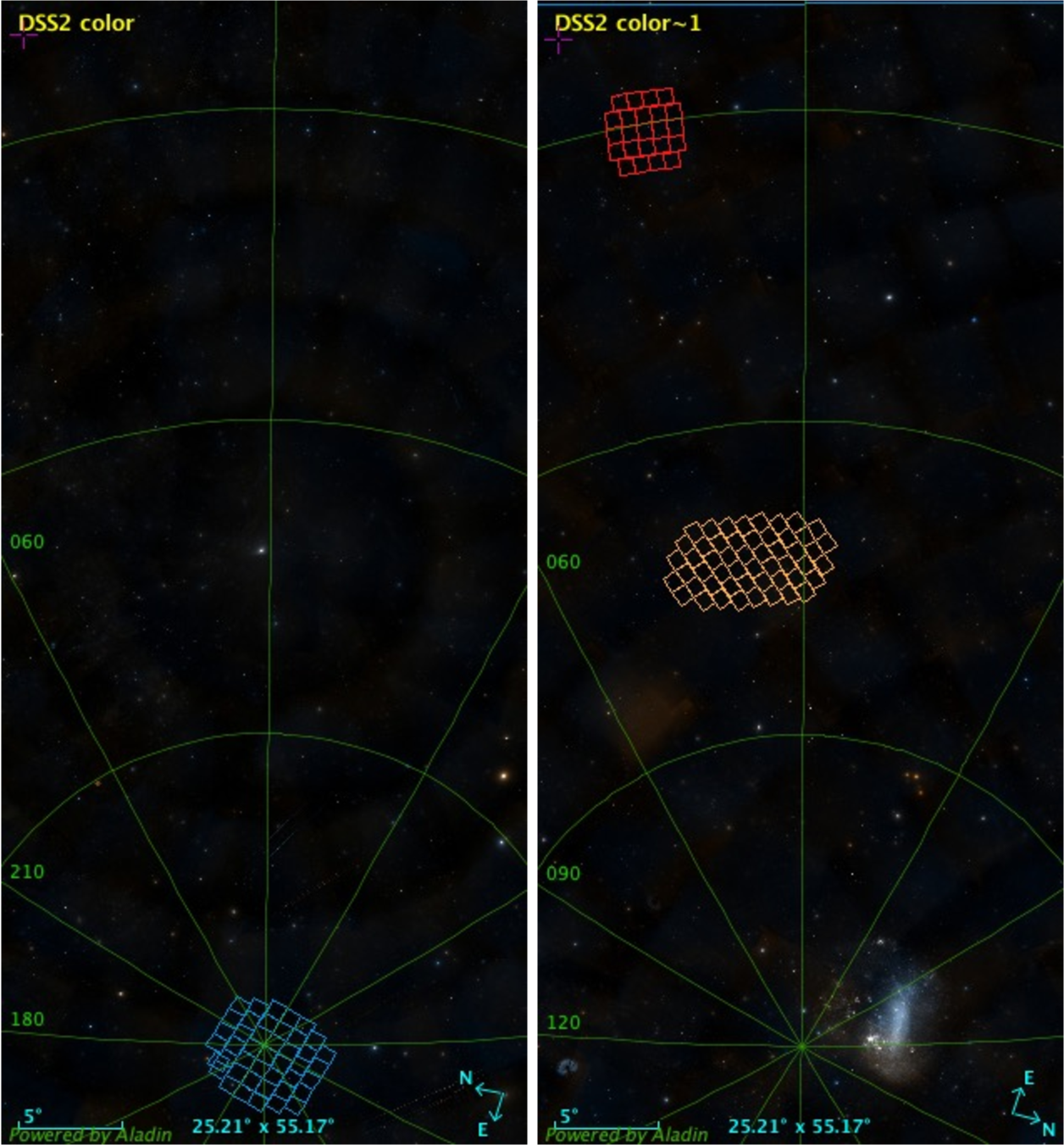
Figure 12: Footprints of the Q1 visits to the EDFs shown on the sky in ecliptic coordinates overlaid on two 25^∘ $\times$ 55^∘ cut-outs of a full-sky Digitized Sky Survey 2 optical image generated by the CDS. Left: A strip of the northern ecliptic hemisphere down to $+45^{\circ}$, showing EDF-N (blue) at the ecliptic pole in the Draco constellation; one of its fields is noticeably out of the regular pattern in order to avoid the bright 42 Dra star. Right: A strip of the southern ecliptic hemisphere down to $-45^{\circ}$ showing EDF-F (red) in the Fornax constellation and EDF-S (orange) in the Dorado constellation. The Large Magellanic Cloud is noticeable close to the ecliptic pole.

A.1 Euclid Deep Field North (Q1 visit)

# Region file format: DS9 version 4.1
global color=green dashlist=8 3 width=1 font="helvetica 10 normal roman" select=1 highlite=1 dash=0 fixed=0 edit=1 move=1 delete=1 include=1 source=1
icrs
polygon(264.893501,+66.876904, 266.545798,+67.314562, 265.507842,+67.901955, 263.834235,+67.453547)
polygon(266.544700,+67.314397, 268.257279,+67.734528, 267.243764,+68.332679, 265.506130,+67.901740)
polygon(268.256414,+67.734214, 270.029657,+68.135953, 269.045117,+68.744752, 267.242481,+68.332262)
polygon(270.502410,+67.829132, 272.320057,+68.206349, 271.394840,+68.828130, 269.543423,+68.440658)
polygon(269.219916,+67.130327, 270.963701,+67.521848, 270.029895,+68.136053, 268.256746,+67.734290)
polygon(267.533196,+66.720617, 269.220313,+67.130413, 268.257279,+67.734528, 266.544918,+67.314341)
polygon(265.902932,+66.293425, 267.533720,+66.720655, 266.545649,+67.314451, 264.892984,+66.876888)
polygon(263.820789,+66.137120, 265.405108,+66.585950, 264.371331,+67.166150, 262.769005,+66.706754)
polygon(262.808185,+65.390331, 264.329254,+65.849557, 263.301380,+66.422788, 261.765345,+65.953277)
polygon(263.805122,+64.820743, 265.310362,+65.269873, 264.328021,+65.849776, 262.806711,+65.390701)
polygon(264.824612,+65.560626, 266.390752,+65.999246, 265.404353,+66.585959, 263.819725,+66.137214)
polygon(266.866432,+65.703672, 268.475126,+66.120927, 267.533453,+66.720621, 265.902671,+66.293440)
polygon(268.474876,+66.120895, 270.136287,+66.520851, 269.220316,+67.130413, 267.533441,+66.720588)
polygon(270.136224,+66.520821, 271.850469,+66.902624, 270.963788,+67.521942, 269.220117,+67.130370)
polygon(271.412680,+67.212635, 273.196736,+67.580074, 272.320148,+68.206674, 270.502730,+67.829417)
polygon(272.764139,+67.893364, 274.621719,+68.245300, 273.759234,+68.879416, 271.863561,+68.517596)
polygon(273.617937,+67.265067, 275.437972,+67.607764, 274.621509,+68.245992, 272.764312,+67.893961)
polygon(274.427855,+66.632410, 276.211277,+66.966355, 275.437265,+67.608373, 273.617658,+67.265539)
polygon(275.197039,+65.995778, 276.944859,+66.321414, 276.210339,+66.966922, 274.427094,+66.632791)
polygon(273.099339,+65.965181, 274.817518,+66.314505, 274.027754,+66.949606, 272.276962,+66.591357)
polygon(272.277219,+66.591202, 274.028159,+66.949337, 273.196497,+67.580354, 271.412776,+67.212867)
polygon(271.008299,+65.906254, 272.693273,+66.278759, 271.850385,+66.902697, 270.136276,+66.520846)
polygon(269.372777,+65.515706, 271.008299,+65.906254, 270.136276,+66.520846, 268.474905,+66.120879)
polygon(267.786616,+65.108100, 269.372777,+65.515706, 268.474905,+66.120879, 266.866323,+65.703735)
polygon(265.784814,+64.977783, 267.331840,+65.406551, 266.390156,+65.999307, 264.824073,+65.560835)
polygon(264.760317,+64.244671, 266.249360,+64.684150, 265.309510,+65.270192, 263.803987,+64.821216)
polygon(265.676327,+63.662629, 267.148505,+64.092747, 266.248879,+64.684564, 264.759689,+64.245306)
polygon(266.555250,+63.074998, 268.010176,+63.496057, 267.148453,+64.093307, 265.676067,+63.663391)
polygon(268.427292,+63.195235, 269.915229,+63.596656, 269.091858,+64.205114, 267.583946,+63.795147)
polygon(267.583847,+63.794739, 269.091601,+64.204828, 268.231276,+64.808484, 266.703618,+64.389350)
polygon(266.703827,+64.389063, 268.231260,+64.808272, 267.331539,+65.406665, 265.784489,+64.978067)
polygon(268.666110,+64.507050, 270.229780,+64.905528, 269.372861,+65.515801, 267.786500,+65.108130)
polygon(270.229642,+64.905424, 271.839504,+65.286942, 271.008297,+65.906253, 269.372808,+65.515703)
polygon(271.839316,+65.286898, 273.495532,+65.650554, 272.693297,+66.278792, 271.008237,+65.906238)
polygon(273.881753,+65.334963, 275.568086,+65.675908, 274.816856,+66.314735, 273.098688,+65.965322)
polygon(274.776103,+65.125740, 276.460162,+65.456719, 275.737758,+66.099857, 274.021387,+65.760637)
polygon(272.631954,+64.663143, 274.259684,+65.018390, 273.495276,+65.650576, 271.839134,+65.286855)
polygon(271.048118,+64.290415, 272.632668,+64.663195, 271.839622,+65.286855, 270.229663,+64.905425)
polygon(269.507512,+63.900998, 271.048631,+64.290659, 270.229950,+64.905531, 268.666185,+64.507145)
polygon(270.313093,+63.290203, 271.831779,+63.671408, 271.048942,+64.290683, 269.507726,+63.901191)
polygon(271.830621,+63.671074, 273.390062,+64.035531, 272.632668,+64.663195, 271.048137,+64.290417)
polygon(273.388700,+64.035332, 274.988662,+64.382470, 274.259328,+65.018376, 272.631649,+64.663072)
polygon(274.627208,+64.700916, 276.282521,+65.033829, 275.567216,+65.676086, 273.880976,+65.335041)

A.2 Euclid Deep Field South (Q1 visit)

# Region file format: DS9 version 4.1 1860
global color=green dashlist=8 3 width=1 font="helvetica 10 normal roman" select=1 highlite=1 dash=0 fixed=0 edit=1 move=1 delete=1 include=1 source=1
icrs
polygon(55.365656,-48.409852, 55.290812,-49.186124, 56.372854,-49.226311, 56.431187,-48.449491)
polygon(55.291518,-49.184519, 55.213699,-49.960700, 56.312971,-50.001827, 56.373586,-49.225062)
polygon(56.313552,-50.001223, 56.250422,-50.778036, 57.369497,-50.809646, 57.414565,-50.032375)
polygon(57.392655,-50.410546, 57.346300,-51.187750, 58.475886,-51.209195, 58.503568,-50.431609)
polygon(57.436152,-49.633845, 57.391803,-50.411142, 58.502655,-50.431983, 58.529267,-49.654403)
polygon(56.373323,-49.225408, 56.312652,-50.002320, 57.413660,-50.033225, 57.456916,-49.255876)
polygon(56.431157,-48.449620, 56.372858,-49.226546, 57.456422,-49.256664, 57.498134,-48.479363)
polygon(56.487136,-47.673775, 56.431049,-48.450718, 57.498030,-48.480220, 57.538165,-47.702809)
polygon(57.558185,-47.303640, 57.518907,-48.080971, 58.578657,-48.100366, 58.602272,-47.322776)
polygon(57.518854,-48.080412, 57.477918,-48.857712, 58.554018,-48.877576, 58.578519,-48.099957)
polygon(57.478188,-48.857135, 57.435615,-49.634420, 58.528756,-49.654843, 58.554207,-48.877152)
polygon(58.546849,-49.104042, 58.520982,-49.881765, 59.619863,-49.892023, 59.628506,-49.114226)
polygon(58.521281,-49.881409, 58.494198,-50.659020, 59.611274,-50.669641, 59.620271,-49.891863)
polygon(58.494853,-50.658750, 58.466564,-51.436428, 59.602462,-51.447240, 59.611908,-50.669504)
polygon(59.614373,-50.367278, 59.604859,-51.145118, 60.733611,-51.145253, 60.724482,-50.367411)
polygon(59.623145,-49.589565, 59.614122,-50.367378, 60.724283,-50.367489, 60.715546,-49.589714)
polygon(59.631601,-48.811896, 59.623070,-49.589711, 60.715365,-49.589667, 60.706904,-48.811874)
polygon(58.571568,-48.326777, 58.546638,-49.104359, 59.628323,-49.114413, 59.636614,-48.336618)
polygon(58.595350,-47.549380, 58.571559,-48.327012, 59.636582,-48.336745, 59.644464,-47.558945)
polygon(58.618388,-46.772027, 58.595513,-47.549662, 59.644733,-47.559187, 59.652307,-46.781375)
polygon(59.654821,-46.478762, 59.647478,-47.256514, 60.690842,-47.256413, 60.683054,-46.478547)
polygon(59.647353,-47.256446, 59.639703,-48.034217, 60.698685,-48.034136, 60.690719,-47.256344)
polygon(59.639630,-48.034130, 59.631496,-48.811936, 60.706852,-48.811893, 60.698632,-48.034156)
polygon(60.702587,-48.412256, 60.710933,-49.190081, 61.794182,-49.179992, 61.769221,-48.402358)
polygon(60.710933,-49.190081, 60.719369,-49.967856, 61.820041,-49.957640, 61.794182,-49.179992)
polygon(60.719369,-49.967856, 60.727976,-50.745645, 61.846813,-50.735253, 61.820041,-49.957640)
polygon(61.807086,-49.579576, 61.833189,-50.357189, 62.942370,-50.336534, 62.898522,-49.559221)
polygon(61.781893,-48.801951, 61.807187,-49.579538, 62.898647,-49.559290, 62.856345,-48.781942)
polygon(61.757450,-48.024337, 61.781944,-48.801932, 62.856366,-48.782048, 62.815520,-48.004683)
polygon(60.694429,-47.634438, 60.702587,-48.412256, 61.769221,-48.402358, 61.745133,-47.624745)
polygon(60.686443,-46.856672, 60.694429,-47.634438, 61.745133,-47.624745, 61.721804,-46.847025)
polygon(60.678587,-46.078835, 60.686443,-46.856672, 61.721804,-46.847025, 61.699282,-46.069404)
polygon(61.687600,-45.691436, 61.710067,-46.469112, 62.737627,-46.450246, 62.700753,-45.672814)
polygon(61.710286,-46.469036, 61.733348,-47.246678, 62.775971,-47.227521, 62.737900,-46.450155)
polygon(61.733577,-47.246711, 61.757397,-48.024356, 62.815537,-48.004790, 62.776065,-47.227377)
polygon(62.799976,-47.702391, 62.840325,-48.479760, 63.907321,-48.450208, 63.851063,-47.673247)
polygon(62.840358,-48.479635, 62.881969,-49.256962, 63.965585,-49.226745, 63.907269,-48.449888)
polygon(62.881771,-49.256805, 62.924845,-50.034120, 64.025843,-50.003267, 63.965370,-49.226480)
polygon(63.923974,-48.676258, 63.982844,-49.453143, 65.069941,-49.412751, 64.994248,-48.636457)
polygon(64.958555,-48.259253, 65.032887,-49.035559, 66.109770,-48.985518, 66.019141,-48.210022)
polygon(63.867244,-47.899836, 63.924169,-48.676755, 64.994451,-48.637060, 64.921478,-47.860769)
polygon(63.812115,-47.123350, 63.867145,-47.900316, 64.921335,-47.861371, 64.850946,-47.085019)
polygon(62.760840,-46.925292, 62.799900,-47.702642, 63.850879,-47.673531, 63.796574,-46.896601)
polygon(62.722630,-46.148011, 62.760463,-46.925420, 63.796218,-46.896939, 63.743710,-46.119907)
polygon(62.685424,-45.370797, 62.722143,-46.148283, 63.743230,-46.120281, 63.692455,-45.343247)
polygon(63.706269,-45.570338, 63.757795,-46.347301, 64.781862,-46.309945, 64.716056,-45.533418)
polygon(64.749278,-45.932675, 64.816383,-46.709097, 65.846335,-46.661972, 65.764790,-45.886200)
polygon(63.758487,-46.346856, 63.811721,-47.123813, 64.850569,-47.085691, 64.782542,-46.309293)
polygon(64.817087,-46.708214, 64.886559,-47.484630, 65.931512,-47.436610, 65.847033,-46.660883)
polygon(64.886848,-47.483762, 64.958623,-48.260123, 66.019223,-48.211103, 65.931792,-47.435532)
polygon(65.931750,-47.435656, 66.019236,-48.211209, 67.077617,-48.152500, 66.974519,-47.377796)
polygon(65.846731,-46.661304, 65.931332,-47.436996, 66.974211,-47.379418, 66.874679,-46.604582)

A.3 Euclid Deep Field Fornax (Q1 visit)

# Region file format: DS9 version 4.1
global color=black dashlist=8 3 width=1 font="helvetica 10 normal roman" select=1 highlite=1 dash=0 fixed=0 edit=1 move=1 delete=1 include=1 source=11920
icrs
polygon(50.585853,-27.644678, 50.902896,-28.370438, 51.651550,-28.112633, 51.330259,-27.388680)
polygon(50.902775,-28.370157, 51.223920,-29.095156, 51.977045,-28.835778, 51.651435,-28.112564)
polygon(51.223872,-29.094851, 51.549421,-29.819124, 52.307059,-29.558040, 51.977039,-28.835567)
polygon(51.928784,-29.688937, 52.261115,-30.411604, 53.021536,-30.146543, 52.684516,-29.425819)
polygon(51.977005,-28.835685, 52.307026,-29.558158, 53.060758,-29.292837, 52.726389,-28.572241)
polygon(51.651435,-28.112564, 51.977045,-28.835778, 52.726315,-28.572265, 52.396513,-27.850868)
polygon(51.330144,-27.388611, 51.651550,-28.112633, 52.396513,-27.850868, 52.071013,-27.128622)
polygon(50.643457,-26.791823, 50.958647,-27.517318, 51.701255,-27.259222, 51.382031,-26.535410)
polygon(51.381611,-26.535441, 51.701065,-27.259178, 52.440171,-26.997106, 52.116833,-26.275027)
polygon(52.070938,-27.128647, 52.396513,-27.850868, 53.137897,-27.585053, 52.808298,-26.864604)
polygon(52.396513,-27.850868, 52.726315,-28.572265, 53.471935,-28.304710, 53.137897,-27.585053)
polygon(52.726315,-28.572265, 53.060724,-29.292954, 53.810546,-29.023558, 53.471935,-28.304710)
polygon(52.684335,-29.425985, 53.021211,-30.146756, 53.777552,-29.877536, 53.436251,-29.158735)
polygon(53.436030,-29.158806, 53.777186,-29.877654, 54.529491,-29.604313, 54.183935,-28.887325)
polygon(53.471860,-28.304734, 53.810472,-29.023581, 54.556487,-28.750127, 54.213657,-28.033135)
polygon(53.137897,-27.585053, 53.471935,-28.304710, 54.213769,-28.033206, 53.875667,-27.315354)
polygon(52.808222,-26.864628, 53.137935,-27.585148, 53.875704,-27.315448, 53.542138,-26.596771)
polygon(52.116452,-26.275149, 52.439944,-26.997179, 53.175612,-26.731160, 52.848223,-26.010814)
polygon(52.847955,-26.011004, 53.175459,-26.731420, 53.907637,-26.461622, 53.576402,-25.742964)
polygon(53.542024,-26.596913, 53.875666,-27.315566, 54.609895,-27.042002, 54.272409,-26.325098)
polygon(53.875667,-27.315354, 54.213769,-28.033206, 54.951906,-27.757769, 54.609861,-27.041696)
polygon(54.213657,-28.033135, 54.556301,-28.750079, 55.298427,-28.472743, 54.951646,-27.757531)
polygon(54.183674,-28.887301, 54.529085,-29.604334, 55.277398,-29.326907, 54.927677,-28.611815)

References

- Abbott et al. (2018) Abbott, T. M. C., Abdalla, F. B., Allam, S., et al. 2018, ApJS, 239, 18
- Abbott et al. (2021) Abbott, T. M. C., Adamów, M., Aguena, M., et al. 2021, ApJS, 255, 20
- Abdalla et al. (2008) Abdalla, F. B., Amara, A., Capak, P., et al. 2008, MNRAS, 387, 969
- Bertin (2006) Bertin, E. 2006, in ASP Conf. Ser., Vol. 351, Astronomical Data Analysis Software and Systems XV, ed. C. Gabriel, C. Arviset, D. Ponz, & S. Enrique, 112
- Bertin (2010) Bertin, E. 2010, SWarp: Resampling and Co-adding FITS Images Together, Astrophysics Source Code Library, record ascl:1010.068
- Bertin (2011) Bertin, E. 2011, in ASP Conf. Ser., Vol. 442, Astronomical Data Analysis Software and Systems XX, ed. I. N. Evans, A. Accomazzi, D. J. Mink, & A. H. Rots, 435
- Bertin et al. (2002) Bertin, E., Mellier, Y., Radovich, M., et al. 2002, ASP Conf. Ser., 281, 228
- Bohlin et al. (2020) Bohlin, R. C., Hubeny, I., & Rauch, T. 2020, AJ, 160, 21
- Bosch et al. (2019) Bosch, J., AlSayyad, Y., Armstrong, R., et al. 2019, in ASP Conf. Ser., Vol. 523, Astronomical Data Analysis Software and Systems XXVII, ed. P. J. Teuben, M. W. Pound, B. A. Thomas, & E. M. Warner, 521
- Bosch et al. (2018) Bosch, J., Armstrong, R., Bickerton, S., et al. 2018, PASJ, 70, S5
- Boulade et al. (1998) Boulade, O., Vigroux, L. G., Charlot, X., et al. 1998, in Society of Photo-Optical Instrumentation Engineers (SPIE) Conference Series, Vol. 3355, Optical Astronomical Instrumentation, ed. S. D’Odorico, 614–625
- Cardelli et al. (1989) Cardelli, J. A., Clayton, G. C., & Mathis, J. S. 1989, ApJ, 345, 245
- Chambers et al. (2016) Chambers, K. C., Magnier, E. A., Metcalfe, N., et al. 2016, arXiv:1612.05560
- Darnell et al. (2009) Darnell, T., Bertin, E., Gower, M., et al. 2009, in Astronomical Society of the Pacific Conference Series, Vol. 411, Astronomical Data Analysis Software and Systems XVIII, ed. D. A. Bohlender, D. Durand, & P. Dowler, 18
- Desai et al. (2012) Desai, S., Armstrong, R., Mohr, J. J., et al. 2012, ApJ, 757, 83
- Desai et al. (2016) Desai, S., Mohr, J. J., Bertin, E., Kümmel, M., & Wetzstein, M. 2016, Astronomy and Computing, 16, 67
- Desai et al. (2015) Desai, S., Mohr, J. J., Henderson, R., et al. 2015, Journal of Instrumentation, 10, C06014
- Duffy et al. (2025) Duffy, C., Cappellaro, E., Botticella, M., et al. 2025, A&A, submitted
- Eriksen & Hoekstra (2018) Eriksen, M. & Hoekstra, H. 2018, MNRAS, 477, 3433
- Euclid Collaboration: Bergamini et al. (2025) Euclid Collaboration: Bergamini, P., Meneghetti, M., Acebron, A., et al. 2025, A&A, submitted
- Euclid Collaboration: Bisigello et al. (2025) Euclid Collaboration: Bisigello, L., Rodighiero, G., Fotopoulou, S., et al. 2025, A&A, submitted
- Euclid Collaboration: Busillo et al. (2025) Euclid Collaboration: Busillo, V., Tortora, C., Metcalf, R., et al. 2025, A&A, submitted
- Euclid Collaboration: Cleland et al. (2025) Euclid Collaboration: Cleland, C., Mei, S., De Lucia, G., et al. 2025, A&A, submitted
- Euclid Collaboration: Copin et al. (2025) Euclid Collaboration: Copin, Y., Fumana, M., Mancini, C., et al. 2025, A&A, submitted
- Euclid Collaboration: Corcho-Caballero et al. (2025) Euclid Collaboration: Corcho-Caballero, P., Ascasibar, Y., Verdoes Kleijn, G., et al. 2025, A&A, submitted
- Euclid Collaboration: Cropper et al. (2024) Euclid Collaboration: Cropper, M., Al Bahlawan, A., Amiaux, J., et al. 2024, A&A, accepted, arXiv:2405.13492