SUM Parts: Benchmarking Part-Level Semantic Segmentation of Urban Meshes

Abstract

Semantic segmentation in urban scene analysis has mainly focused on images or point clouds, while textured meshes—offering richer spatial representation—remain underexplored. This paper introduces SUM Parts, the first large-scale dataset for urban textured meshes with part-level semantic labels, covering about $2.5\,\text{km}^{2}$ with 21 classes. The dataset was created using our own annotation tool, which supports both face- and texture-based annotations with efficient interactive selection. We also provide a comprehensive evaluation of 3D semantic segmentation and interactive annotation methods on this dataset. Our project page is available at https://tudelft3d.github.io/SUMParts/.

1 Introduction

Semantic segmentation is crucial to understanding urban scenes by accurately classifying objects and improving data usability. Recent advances have led to the development of datasets and methods primarily for images and point clouds [15, 40, 35]. Research on textured meshes has focused mainly on small-scale indoor settings [5, 16, 11], with limited work on large outdoor environments [42, 52, 19, 20]. Furthermore, a critical gap in urban scene understanding is part-level semantic segmentation, which decomposes urban objects into functional components (e.g., windows, chimneys, road markings) following the international CityGML standard [45]. To address this, we introduce the first large-scale benchmark dataset providing part-level semantic labels for urban textured meshes.

Obtaining ground truth labels for urban scene understanding often relies on manual annotation, which is time-consuming and expensive [19]. Labeling large-scale 3D scenes poses significant challenges compared to 2D image annotation, requiring flexible viewpoint management, specialized interaction methods, and advanced rendering techniques. Although considerable research has focused on interactive point cloud annotation [36, 54, 29], efforts to annotate textured meshes [49, 19] remain very sparse. Existing studies often label mesh vertices [16, 31] or faces [49, 19], neglecting the richer details provided by textures.

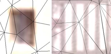
Figure 2: Mesh textures and wireframes (black).

Details such as building windows and road markings are better represented in texture images than in unconstrained mesh faces (see Fig.˜2). To address this, we introduce an efficient interactive tool for textured meshes, enabling both face- and texture-based annotations.

The main contributions are (1) the first large-scale dataset with part-level semantic labels for urban textured meshes, (2) an efficient interactive annotation tool, and (3) a comprehensive analysis of state-of-the-art 3D semantic segmentation and interactive annotation methods.

2 Related work

Annotation for semantic segmentation. Annotation for semantic segmentation is essential in computer vision, leading to the development of various interactive methods for both 2D images and 3D data.

Early interactive image segmentation methods include region-growing [2, 44], contour-based [43], graph-cut [6, 50], and random walk approaches [21]. While effective, they often require significant user input or struggle with complex images. Deep learning models like DEXTR [39] and SAM [27] have advanced the field but depend on large datasets and may perform poorly on unseen categories. Our interactive annotation method for mesh texture images overcomes these limitations, offering greater generalizability without relying on extensive training data.

Interactive 3D annotation uses data like multi-view images, point clouds, and meshes. Manual methods [26] are labor-intensive; graph-cut approaches [36] depend heavily on user input quality; region-based methods [19] can lead to segmentation errors. Deep learning techniques [29, 61] require extensive training data and struggle with new data. In contrast, our unsupervised approach requires no prior labeling and operates independently of the original imagery, using approximate user selections and template matching to enhance efficiency and accuracy in complex 3D scenes.

Semantic 3D urban datasets. While several semantic 3D urban datasets exist for LiDAR and photogrammetric point clouds [24, 53, 3, 34, 10, 35], they lack fine-grained part-level semantics essential for comprehensive urban analysis. This is partly due to inherent point cloud limitations, such as low resolution and missing data from occlusions, which hinder capturing detailed structures and small object boundaries [18]. Additionally, point clouds have larger data volumes than textured meshes, leading to longer processing times and higher storage requirements without added informational benefit. In contrast, textured meshes offer better resolution and completeness, but existing mesh datasets [9, 19] typically lack part-level semantic annotations and cover limited categories or scales, focusing on specific objects [62, 28], which limits their applicability. Moreover, existing annotations frequently overlook the rich texture information in meshes. To address these gaps, we introduce the first part-level benchmark dataset of large-scale urban meshes for comprehensive urban analysis.

3 The SUM parts dataset

We aim to use our developed interactive 3D annotation tool to create ground truth for urban textured meshes. Using Helsinki city’s mesh [4] as input, the output includes meshes with face labels and semantic texture masks. The textured meshes were generated using Bentley’s ContextCapture [57], reconstructed from oblique aerial imagery with a ground sampling distance of approximately $7.5\,\text{cm}$. The annotations were conducted in three representative areas of central Helsinki, comprising 40 tiles of $62,500\,\text{m}^{2}$ each, covering a total area of approximately $2.5\,\text{km}^{2}$.

3.1 Annotation

Our annotation aims to achieve precise semantic labeling with significantly improved efficiency for urban meshes. Our tool features two main modules for part-level semantic annotation: face-based annotation for triangle faces and texture-based annotation for texture pixels. We enhance the efficiency of both modules by incorporating interactive selection and template-matching strategies. We invited five individuals with experience in remote sensing to manually annotate the dataset using our tool: two focused on face-based annotation, two on texture pixel-based annotation, and one reviewed and corrected the annotations. The entire annotation process took approximately 640 hours in total.

3.1.1 Face-based annotation

The face-based annotation aims to assign labels to each face through user interaction, using tools like brushes, strokes, and lassos. To minimize interactions, we developed interactive 3D selection and template-matching algorithms. We first over-segment the mesh into planar segments via region growing, enabling quick selection of large areas, while protrusions are selected semi-automatically based on geometric features. Leveraging the repetitive nature of urban structures, we use structural features for template matching to facilitate rapid annotation.

1) Interactive 3D selection. We propose an interactive protrusion extraction method to address the challenges in over-segmented urban textured meshes, which often struggle with non-planar areas, sharp features, and small-scale structures due to under- or over-segmentation [20]. Our method aims to efficiently identify protrusions not part of the support plane, similar to foreground-background separation in image segmentation [50]. It involves two main steps that work seamlessly to enhance annotation efficiency.

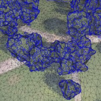
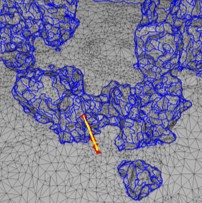
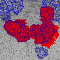
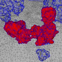
(a) Input	(b) Lasso/Stroke	(c) Candidates	(d) Protrusions

Figure 3: Interactive 3D selection. The user performs a lasso (green) or stroke selection (yellow) (b), which generates candidate faces (red) (c). Binary labeling is then applied to these candidate faces to extract protrusions (red) (d).

First, during interactive selection, users employ a lasso or stroke to generate candidate faces for labeling. The algorithm distinguishes these inputs based on the ratio of contour endpoints’ distance to the bounding box diagonal and ensures consistent candidate face extraction. For lasso input, all planar segments within the lasso are selected. For stroke input, the selection expands to neighboring faces along the stroke’s path, selecting their corresponding planar segments as candidate faces (see Fig.˜3).

Second, we formulate protrusion selection as a binary labeling problem $l^{f}=\{\text{support plane},\text{protrusion}\}$. The candidate segments $\{f_{i}\}$ are ordered by area, with the largest serving as the support plane. We construct a dual graph $\mathcal{G}^{f}=\{\nu^{f},\xi^{f}\}$ for all candidate faces $f=\{f_{i}\}$ each represented by a node in the graph and connected to adjacent faces by graph edges.

The data term $D^{f}$ evaluates the likelihood that face $f_{i}$ belongs to a protrusion:

$$D^{f}(l^{f}_{i})=\eta\times\begin{cases}p_{i}&\text{if }l^{f}_{i}\text{ is support plane},\\ 1-p_{i}&\text{if }l^{f}_{i}\text{ is protrusion},\end{cases}$$

where $\eta$ modulates sensitivity to various geometric characteristics, and $p_{i}=d_{i}+\omega_{i}\theta_{i}$ is the protrusion score. Here, $d_{i}$ is the maximum distance from face $f_{i}$ to the support plane $P^{f}_{k}$; $\theta_{i}$ is the minimum angle that quantifies the orientation deviation between the normals of face $f_{i}$ and the support plane $P^{f}_{k}$, and $\omega_{i}$ is defined as:

$$\omega_{i}=\begin{cases}1&\text{if }d_{i}>1,\\ 1-d_{i}&\text{otherwise}.\end{cases}$$

The smoothness term $V^{f}$ measures geometric similarity between adjacent faces:

$$V^{f}(l^{f}_{i},l^{f}_{j})=R_{i,j}\cdot 1_{\{l^{f}_{i}\neq l^{f}_{j}\}},$$

where $z_{\max}$ and $z_{\min}$ correspond to the range of z-values of all vertices in $\{f_{i}\}$, and $R_{i,j}=1-\min\left(1,\dfrac{2|r_{i}-r_{j}|}{z_{\max}-z_{\min}}\right)$, and $r_{i}$, $r_{j}$ are shrinking ball radii computed via the 3D medial axis transform [56]. This accounts for local geometric consistency. By combining the above terms, we define the objective function as:

$$E^{f}(l^{f})=\sum_{i}D^{f}(l^{f}_{i})+\lambda^{f}\sum_{\{i,j\}}V^{f}(l^{f}_{i},l^{f}_{j}),$$

which we minimize using a graph-cut algorithm [7]. The parameter $\lambda^{f}$ adjusts the weight of the smoothness term, controlling the influence of geometric similarity.

2) 3D template matching. To leverage repetitive structures in urban scenes and reduce annotation efforts, we employ 3D template matching using structural awareness features from user-selected faces, matching them with similar structures in the scene. This strategy unifies both planar segment and protrusion matching.

(a) User-selected segment

(b) Matched segments

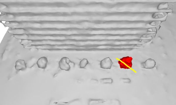
(c) User-selected protrusion

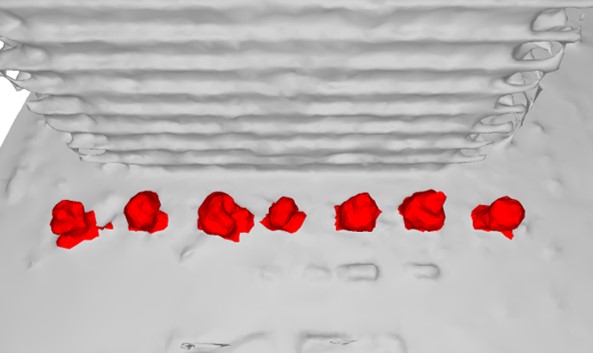
(d) Matched protrusions

Figure 4: 3D template matching. When the user selects a planar segment by clicking on it (a), the matched segments are automatically identified (b). A similar matching process also applies to protrusions via a user-drawn stroke, as shown in (c) and (d).

For planar segment matching (see Fig.˜4(a) to Fig.˜4(b)), we treat the user-selected segment $P^{(t)}$ as a template and compare it with candidate segments $\{P^{(c)}_{k}\}$ based on feature similarity. We assess characteristics such as geometric homogeneity (comparing surface areas), spatial distribution (weighted average heights), orientation (vertical orientations), shape sphericity (based on eigenvalues), and optionally photometric coherence (similarity in color), which constitute a feature vector $\mathbf{F}^{(\text{seg})}$. A match is determined when the Euclidean norm $\|\mathbf{F}^{(\text{seg})}\|<\epsilon^{(\text{seg})}$ where $\epsilon^{(\text{seg})}$ is user-defined depending on input quality.

In protrusion matching (see Fig.˜4(c) to Fig.˜4(d)), we use the user-extracted protrusions as templates to find similar structures. We first decompose the template protrusion into planar segments and match them with segments in the scene. The matched segments serve as seeds, which are expanded to neighboring segments to generate candidate regions. We apply spatial and segment scale constraints to limit the expansion:

$$\left\|O^{(e)}_{k}-O^{(a)}_{j}\right\|<\sqrt{s}\cdot\max_{i}\left\|O^{(t)}-O^{(t)}_{i}\right\|,$$

where $O^{(e)}_{k}$ is the center of the seed segment $P^{(e)}_{k}$, $O^{(a)}_{j}$ is the center of face $f^{(a)}_{j}$ in the neighboring segment $P^{(a)}_{k}$, $O^{(t)}$ is the center of the template faces $f^{(t)}$, $O^{(t)}_{i}$ is the center of individual template face $f^{(t)}_{i}$, and $s$ is the structural scale parameter controlling the expansion based on the template size. The segment scale constraint ensures that neighboring segments are comparable in size to the templates:

$$\frac{A^{(a)}_{k}}{A^{(e)}_{k}}<s\cdot\frac{\max_{j}A^{(t)}_{j}}{\min_{j}A^{(t)}_{j}},$$

where $A^{(a)}_{k}$ and $A^{(e)}_{k}$ are the areas of the neighboring segment $P^{(a)}_{k}$ and seed segment $P^{(e)}_{k}$, respectively, and $A^{(t)}_{j}$ are the areas of the template’s planar segments.

We then extract candidate protrusions based on structural features such as spatial compactness (comparing the volume occupied by the protrusion relative to its bounding box), surface complexity (assessed by the number of planar segments composing the protrusion), and eigenvalue-based characteristics like linearity, planarity, and sphericity (derived from the covariance of vertex positions). These features form a vector $\mathbf{F}^{(\text{str})}$, and a match is accepted when the Euclidean norm $\|\mathbf{F^{(\text{str})}}\|<\epsilon^{(str)}$, where $\epsilon^{(str)}$ is determined by user interaction and data quality.

3.1.2 Texture-based annotation

Mesh textures capture fine details more effectively and avoid the redundancies and discontinuities often found in image-based annotations. However, direct texture annotation is challenging due to discontinuities and computational demands. To address this, we propose a mesh texture annotation strategy based on planar segments, allowing flexible splitting and merging of segments. Our efficient interactive annotation leverages local region extraction and 2D template matching, operating under the assumption that semantic components consist of superpixels with similar geometric and color features.

1) Interactive 2D selection. We aim to capture the region of interest through user clicks. Unlike traditional methods, our approach requires only positive samples. As shown in Fig.˜5, our method consists of two main steps: local expansion and fine segmentation.

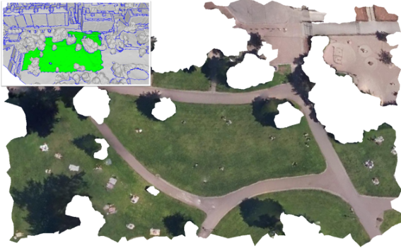
(a) Textured planar segment

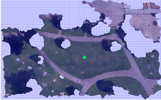
(b) User’s click selection

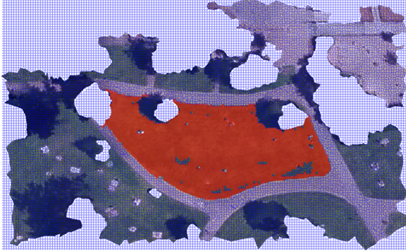
(c) Local expansion

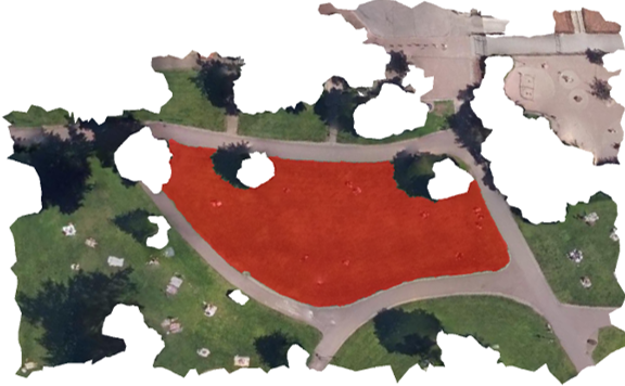
(d) Fine segmentation

Figure 5: Interactive 2D selection. The user selects a texture segment (green) (a). Superpixels are generated (blue), and the user clicks on the region of interest (green star) (b). This triggers local expansion, yielding a coarse segmentation (red) (c), followed by fine segmentation for the final selection (red) (d).

In the first local expansion step, we expand the seed superpixels selected by user clicks to encompass the entire area of interest. We first apply Simple Linear Iterative Clustering (SLIC) [1] to generate homogeneous superpixels from the textured planar segment. We then construct a local adjacency graph $\mathcal{G}^{s}=\{\nu^{s},\xi^{s}\}$, where each superpixel is a node connected to its adjacent superpixels. We formulate the expansion as a binary labeling problem $l^{s}=\{\text{similar},\text{non-similar}\}$, aiming to label adjacent superpixels based on their similarity to the initial seed superpixel $S_{0}$. The data term $D^{s}$ measures this similarity using the average Wasserstein distance of their Gaussian mixture models (GMMs) over the RGB channels:

$$D^{s}(l^{s}_{j})=\alpha\times\begin{cases}1-w_{j}&\text{if }l^{s}_{j}\text{ is non-similar},\\ w_{j}&\text{if }l^{s}_{j}\text{ is similar},\end{cases}$$

where $w_{j}=\frac{1}{K}\sum_{k=1}^{K}W(G_{k}(S_{j}),G_{k}(S_{0}))$, $K=3$ is the number of channels, and $W$ denotes the Wasserstein distance between the GMMs of the superpixels in each channel. The smoothness term $V^{s}$ captures color differences between neighboring superpixels:

$$V^{s}(l^{s}_{j},l^{s}_{j^{\prime}})=H_{j,j^{\prime}}\cdot 1_{\{l^{s}_{j}\neq l^{s}_{j^{\prime}}\}},$$

where $H_{j,j^{\prime}}=|\rho_{j}-\rho_{j^{\prime}}|$, with $\rho_{j}$ being the color distance (CIEDE2000 [38]) between superpixel $S_{j}$ and the seed $S_{0}$. The energy function combines these terms:

$$E^{s}(l^{s})=\sum_{j\in\nu^{s}}D^{s}(l^{s}_{j})+\lambda^{s}\sum_{\{j,j^{\prime}\}\in\xi^{s}}V^{s}(l^{s}_{j},l^{s}_{j^{\prime}}),$$

where $\lambda^{s}$ adjusts the weight of $V^{s}$. We minimize this energy using graph cuts [7] to obtain the expanded region.

Second, we perform fine segmentation to refine the coarse results from the local expansion,

which may be imprecise at object boundaries due to superpixel resolution and user input. Building on GrabCut [50], we perform detailed pixel-level segmentation using foreground samples while automatically generating background samples from the area beyond the optimal bounding box of the coarse results.

2) 2D template matching. To improve annotation efficiency for texture images with repetitive structures like windows and road markings, we adopt fast-matching techniques based on 2D structural awareness. We use user-defined templates to find similar structures within the textured planar segment. The template can be a user-selected region or any arbitrary shape drawn by the user. Normalized Cross-Correlation (NCC) [8] can be used to identify potential matches. However, NCC performs poorly when faced with rotation and scale changes, especially in 3D urban scenes with varying orientations (see Fig.˜6). To overcome this, we propose a region-based template matching approach by extracting structural features from the region $R^{(t)}$ created by local expansion and matching them to similar regions within the textured planar segments. We calculate the Gaussian Mixture Model (GMM) $G_{k}(R^{(t)})$ of the user-selected region. We then use the Wasserstein distance to filter candidate superpixels:

$$W(G_{k}(R^{(t)}),G_{k}(S^{(c)}_{i}))<\epsilon^{\text{seed}},$$

where $\epsilon^{\text{seed}}$ is a user-adjustable threshold, and $G_{k}(S^{(c)}_{i})$ represents the GMM of candidate superpixel $S^{(c)}_{i}$. From the qualified superpixels, we extract candidate regions $\{R^{(c)}_{i}\}$ and compute their similarity to the template region to form a feature vector $\mathbf{F}^{(\text{reg})}$, which includes: shape index (measuring elongation or flatness), shape regularity (how well the region fills its bounding box), contextual features (similarity in internal and external color distributions). We accept matches where the Euclidean norm $\|\mathbf{F}^{(\text{reg})}\|<\epsilon^{\text{reg}}$, with $\epsilon^{\text{reg}}$ depending on user input and image resolution. We also constrain the scale of matching regions using a scaling range based on the number of template pixels:

$$s^{\text{range}}\in\left[\frac{N(R^{(t)})}{s^{\text{reg}}},s^{\text{reg}}\cdot N(R^{(t)})\right],$$

where $N(R^{(t)})$ is the number of pixels in the template region, and $s^{\text{reg}}$ is the scaling factor. Notably, unlike NCC-based template matching, our method offers rotational and scale invariance, allowing it to match targets of varying orientation and size within textured planar segments.

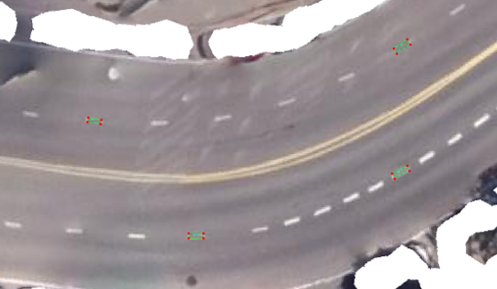
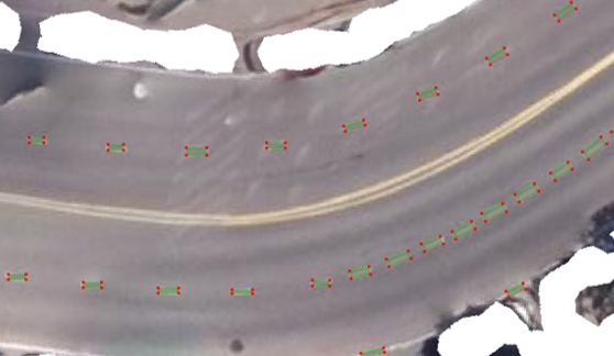
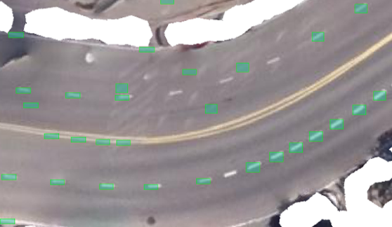
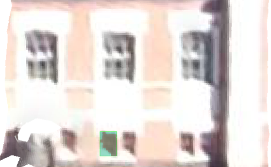
(a) Selected template

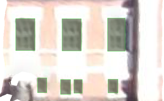
(b) Our matching

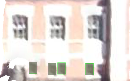
(c) NCC matching

Figure 6: 2D template matching: Extracted regions with green bounding boxes: top shows optimal bounding boxes (rotational invariance), bottom shows vertically aligned bounding boxes (scale invariance) compared to NCC-based methods [8].

3.2 Label definition

In the semantic annotation process, we defined two label types: face and pixel labels. Each triangle mesh face is assigned one of 13 semantic face labels listed in the top part of Tab.˜1. Based on these, we defined pixel labels for mesh textures to capture part-level details, introducing 8 new categories shown in the bottom part of Tab.˜1. We differentiate between two types of labeled scenes: meshes with only face labels, featuring 12 semantic classes (excluding ‘unclassified’), and meshes with both face and pixel labels, comprising 19 semantic classes (excluding ‘unclassified’, and ‘terrain’ as these are broken down into more specific pixel labels). Fig.˜7 show the details of class distribution.

Color	Name	Explanation
	terrain	Ground surfaces.
	high vegetation	Tall plants such as trees.
	water	Bodies of water.
	car	Road vehicles.
	boat	Watercraft.
	wall	Vertical barriers.
	roof surface	Building roofs.
	facade surface	Exterior building walls.
	chimney	Roof vents for smoke.
	dormer	Roof projections.
	balcony	Outdoor platforms on buildings.
	roof installation	Fixtures on roofs.
	window	Glass openings in buildings.
	door	Entrances to buildings.
	low vegetation	Short plants like grass.
	impervious surface	Non-permeable surfaces.
	road	Vehicular paths.
	road marking	Markings on roads.
	cycle lane	Bicycle paths.
	sidewalk	Pedestrian paths beside roads.
	unclassified	Elements not classified elsewhere.

Table 1: The top 12 are face label definitions, the middle 8 are pixel label definitions, and the last ‘unclassified’ applies to both.

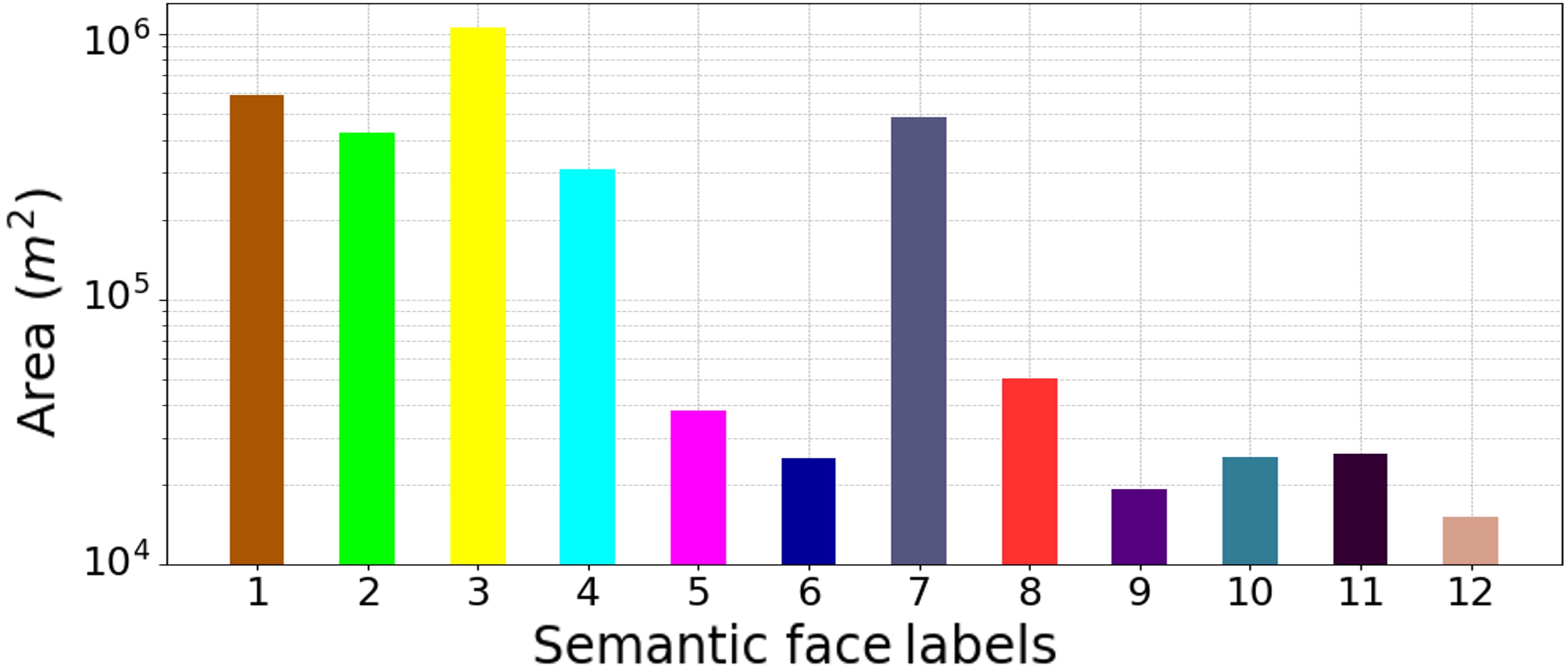
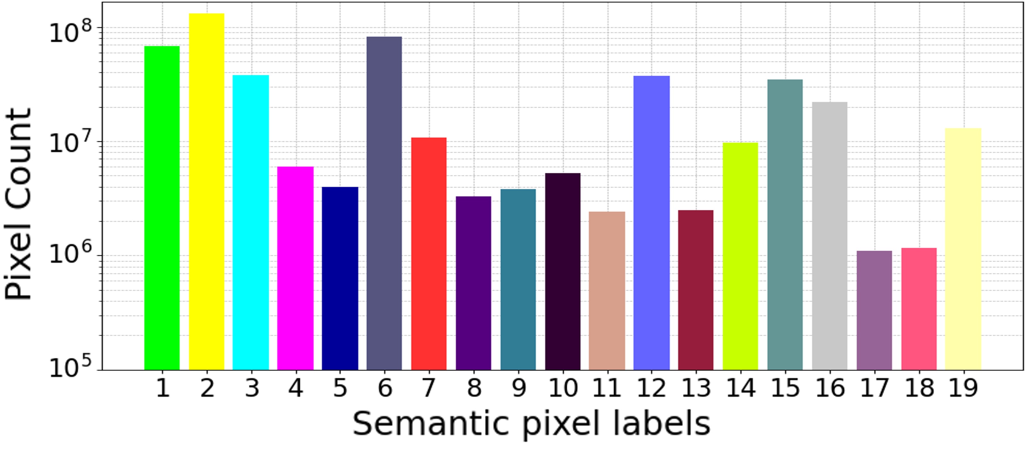
Figure 7: Statistical distribution of semantic classes across the entire dataset for face (top) and pixel-level labels (bottom).

4 Benchmarks

4.1 Evaluation of semantic segmentation

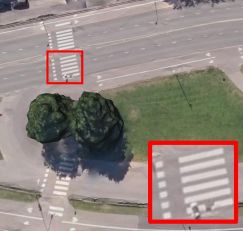
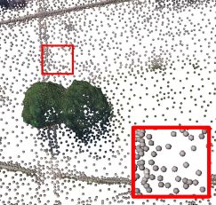
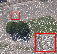
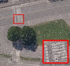
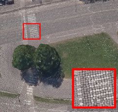
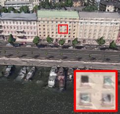
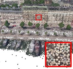
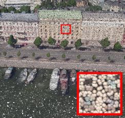
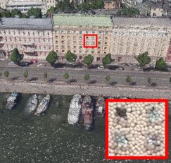
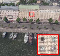
Figure 8: Comparison of mesh sampling methods. From left to right: input meshes, face-centered sampling, random sampling, Poisson-disk sampling [14], and our superpixel texture sampling.

Research shows that semantic segmentation can be performed on point clouds sampled from mesh surfaces [19, 55], mapping results back to meshes via nearest neighbor or voting methods. Traditional sampling methods (e.g., face-centered, random, Poisson-disk [14]) often miss fine details or exhibit density sensitivity issues in complex environments (see Fig.˜8). We apply SLIC [1] over-segmentation on texture images to accurately capture boundaries, then use superpixel centers to generate a texture-based point cloud, ensuring precise semantics, fewer samples, reduced computational load, and efficient pixel-to-point label transfer.

We evaluate state-of-the-art 3D semantic segmentation methods on our datasets, including mesh-based methods like RF-MRF [52], SUM-RF [19], and PSSNet [20], and point cloud based approaches like PointNet [12], PointNet++ [47], superpoint graphs (SPG) [30], SparseConvUnet [22], RandLA-Net [25], KPConv [58], PointNext [48], Point Transformer V3 (PointTransV3) [60], and PointVector [17]. It is worth noting that there are currently no semantic segmentation methods specifically designed for meshes with textured-based pixel labels. These point cloud segmentation methods were evaluated on both the face and pixel labeling tracks. We divide our data into three random splits: 24 tiles for training, 8 for validation, and 8 for testing. To address the class imbalance, we applied class weights to each method, and to reduce randomness in network predictions, results are averaged over five training runs.

We used established semantic segmentation evaluation metrics, conducting a detailed analysis that included Intersection over Union (IoU) per class, overall accuracy (OA), mean accuracy (mAcc), and mean IoU (mIoU). For the face labeling track, we determine the final labels of triangles using a voting method based on point cloud prediction results, with the area of each triangle serving as a weight for semantic evaluation metrics. For the pixel labeling track, we assign final labels to each pixel in the texture image using the nearest neighbor method based on point cloud prediction results, evaluating pixel-level semantic metrics.

	Face Labeling				Pixel Labeling
	Fc.	Rd.	Po.	Sp.	Rd.	Po.	Sp.
PointNet	5.1	8.5	5.1	15.1	2.5	5.7	2.6
PointNet++	27.1	17.3	18.4	33.1	20.6	19.5	24.7
SPG	29.9	29.7	31.5	31.7	16.0	20.0	19.2
SparseUNet	60.5	47.6	38.6	49.9	34.5	13.3	23.3
Randla-net	57.4	49.8	49.1	54.4	36.9	39.9	42.1
KPConv	57.5	56.4	46.5	52.9	38.9	26.1	42.6
PointNext	65.3	51.3	50.4	47.7	42.9	44.7	43.0
PointTransV3	59.1	49.5	51.7	54.0	38.0	36.1	37.8
PointVector	70.0	56.1	52.8	57.1	44.7	45.1	47.9
Average (mIoU)	48.0	40.7	38.2	44.0	30.6	27.8	31.5

Table 2: Evaluation against different sampling strategies on semantic segmentation using mIoU. ‘Fc.’ represents face-centered sampling, ‘Rd.’ random sampling, ‘Po.’ Poisson-disk sampling [14], and ‘Sp.’ superpixel texture sampling. The highest and average mIoUs for each method are highlighted in bold.

1) Face labeling track. The face labeling track includes 12 labels, excluding ‘unclassified’. We evaluated the impact of four mesh point cloud sampling strategies on semantic segmentation. To control point cloud density, the number of points for random and Poisson-disk samples matched the superpixel texture sample size, while face-centered samples always matched the number of mesh faces.

Tab.˜2 shows that using face-centered point clouds leads to optimal performance for most methods. This is because they adapt well to the geometric characteristics of triangulated meshes, where triangle density is lower in flat areas and higher in non-flat areas. Such a distribution enables deep learning networks to learn rich geometric features. However, this does not apply to uniform triangular meshes, indicating that the impact of point cloud sampling density on semantic segmentation is far less significant than the impact of point cloud distribution. The average mIoU in Tab.˜2 also indicates that our proposed superpixel texture sampling method outperforms other mesh sampling methods (except for face-centered point clouds).  Tab.˜3 shows that PointVector [17] surpasses all competing methods with the highest mAcc of 80.7% and mIoU of 70.0%.  Fig.˜9 presents a qualitative analysis of the top three methods.

	Face Labeling Track			Pixel Labeling Track
	Sa.	mAcc	mIoU	Sa.	mAcc	mIoU
RF_MRF	-	45.3	39.5	-	-	-
SUM_RF	-	53.6	46.0	-	-	-
PSSNet	-	56.4	47.0	-	-	-
PointNet	Sp.	22.0	15.1	Sp.	9.8	2.6
PointNet++	Sp.	46.9	33.1	Sp.	35.2	24.7
SPG	Sp.	55.0	31.7	Sp.	34.5	19.2
SparseUNet	Fc.	71.7	60.5	Rd.	45.1	34.5
Randla-net	Fc.	76.3	57.4	Sp.	57.7	42.1
KPConv	Fc.	64.7	57.5	Sp.	58.3	42.6
PointNext	Fc.	77.2	65.3	Po.	57.6	44.7
PointTransV3	Fc.	70.2	59.1	Rd.	54.1	38.0
PointVector	Fc.	80.7	70.0	Sp.	63.8	47.9

Table 3: Evaluation of semantic segmentation performance for face labeling and pixel labeling tracks. ‘Sa.’ represents sampling methods, including ‘Fc.’ for face-centered sampling, ‘Rd.’ for random sampling, ‘Po.’ for Poisson-disk sampling [14], and ‘Sp.’ for superpixel texture sampling. ‘-’ indicates not applicable.

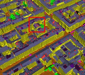
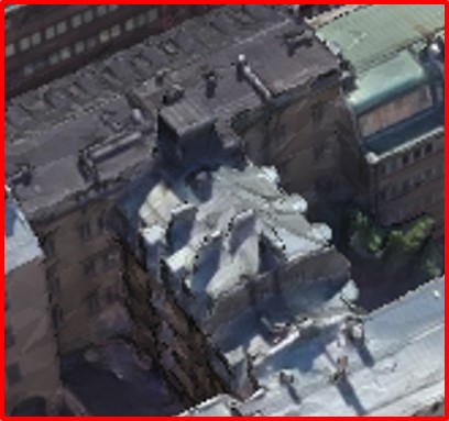
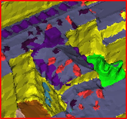
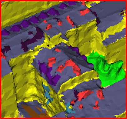
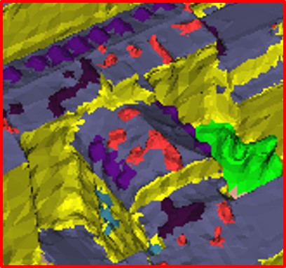
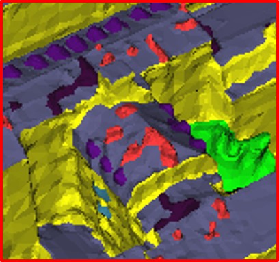
Input	SpUNetFc.	PtNextFc.	PtVectorFc.	Truth
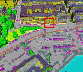
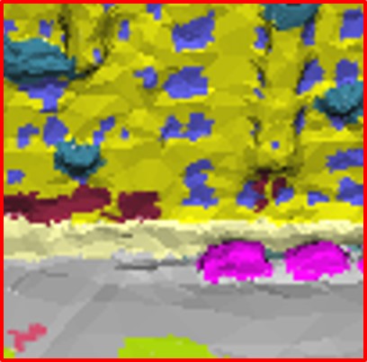
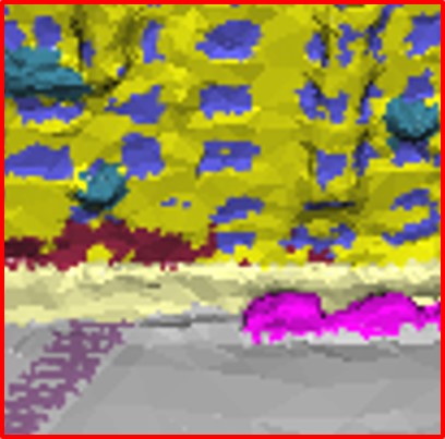
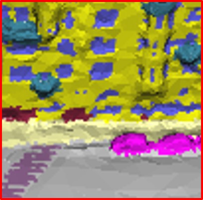
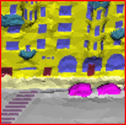
Input	KPConvSp.	PtNextPo.	PtVectorSp.	Truth

Figure 9: Qualitative analysis of face and pixel labeling. The top two rows show the three best methods for face labeling: SparseUNet^Fc. [22], PointNext^Fc. [48], and PointVector^Fc. [17]. The bottom two rows show the three best methods for pixel labeling: KPConv^Sp. [58], PointNext^Po. [48], and PointVector^Sp. [17]. ‘Fc.’ represents face-centered sampling, ‘Po.’ Poisson-disk sampling [14], and ‘Sp.’ superpixel texture sampling.

2) Pixel labeling track. The pixel labeling track consists of 19 semantic classes, as described in Sec.˜3.2, including all semantic labels except for ‘terrain’ and ‘unclassified’. We evaluated the impact of three sampling methods—random, Poisson-disk, and superpixel texture sampling—on semantic segmentation performance. Because face-centered point clouds cannot represent semantic components with pixel labels, they were excluded from testing.

The average mIoU in Tab.˜2 shows most methods achieve optimal performance with our proposed sampling, which precisely captures the boundaries of part-level objects.  Tab.˜3 shows that PointVector [17] continues to outperform all other methods, achieving a mIoU of 47.9%, significantly higher than the others. We also conducted a qualitative analysis of the top three methods, shown in Fig.˜9.

4.2 Evaluation of interactive annotation

We evaluated existing interactive annotation methods for meshes and textured images in real-world scenarios and proposed new evaluation criteria based on user studies. Traditional metrics like the number of clicks to achieve a certain IoU or Average Precision (AP) do not fully capture annotation efficiency due to limitations in evaluation comprehensiveness, interaction complexity, and efficiency measurement. To address these issues, we developed new evaluation metrics including average mean IoU ($\overline{M}$), average boundary mean IoU ($\overline{B}$), average number of mean user interactions ($\overline{O}$), average user annotation time ($\overline{T}(s)$), and average percentage of using smart interaction tools ($\overline{S}(\%)$).

	$\overline{M}(\%)$	$\overline{B}(\%)$	$\overline{O}$	$\overline{T}(s)$	$\overline{S}(\%)$
Manual	-	-	6754	4183.2	-
Segment-based	91.6	74.7	6119	3565.8	-
Ours	92.2	75.0	2992	2992.1	83.0
Manual	-	-	653	777.1	-
GrabCut	88.1	47.1	711	780.9	30.2
SAM	84.4	29.8	716	640.6	71.7
SimpleClick	81.4	30.9	252	861.3	-
Ours	87.9	49.3	582	663.3	40.3

Table 4: Comprehensive performance evaluation of interactive face (top) and texture image annotation (bottom) methods across different test scenarios. The highest values are given in bold.

In our experiments, five users were invited to annotate four representative scenes for face annotation and six for texture annotation using various methods. For interactive face annotation, we compared our method with manual [52] and segment-based interactive annotation [19]. Our method outperformed both in all metrics, reducing the number of interactions and annotation time significantly—about 1.73 times faster than manual annotation and 1.32 times faster than segment-based methods (see Tab.˜4 top and Fig.˜10). The smart interaction ratio exceeded 80% in most scenarios, indicating minimal manual intervention was needed.

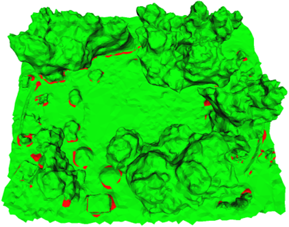
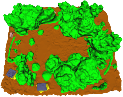
Input	Segment-based	Ours	Manual

Figure 10: Errors (red) in interactive face annotation.

For interactive texture annotation, we compared with manual annotation, GrabCut [50], SAM [27], and SimpleClick [37]. Our method surpassed deep learning methods in annotation quality and was comparable to the fastest annotation times of SAM (see Tab.˜4 bottom and Fig.˜11). It excelled in boundary accuracy due to our fine segmentation and template matching.

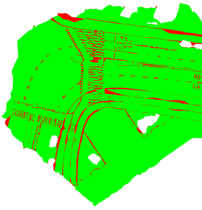
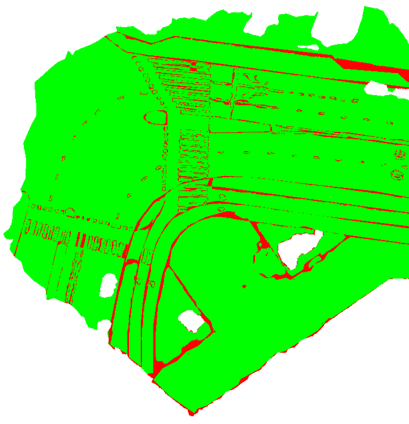
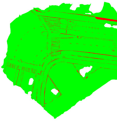
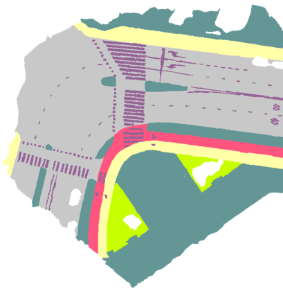
Input	GrabCut	Simclick	SAM	Ours	Manual

Figure 11: Boundary errors (red) in interactive texture annotation.

Notably, for objects with regular shapes or repetitive structures, interactive clicking can be inefficient, requiring users to manually trace shape boundaries for higher accuracy. Our method addresses this by enabling efficient annotation of similar structures using reusable templates, reducing repetitive interactions.

4.3 Sensitivity analysis

Conducting ablation studies on energy function-based methods is challenging due to the high interdependence among terms and the complexity of the optimization, complicating the evaluation of individual parts. We conducted a qualitative analysis to assess the impact of parameter adjustments and data quality on our method’s outcomes.

In face-based analysis, increasing the balance parameter $\lambda^{f}$ improves object boundary clarity while adjusting segment matching thresholds ($\epsilon^{(\text{seg})}$ and $\epsilon^{(\text{str})}$) enhances coverage of repetitive structures (see Fig.˜12 top). Our method demonstrates significant noise tolerance, accurately extracting protrusions despite added Gaussian noise, which is crucial for effective template matching (see Fig.˜13 top).

In texture-based analysis, a larger balance parameter $\lambda^{s}$ smooths local regions, while higher thresholds ($\epsilon^{\text{seed}}$ and $\epsilon^{\text{reg}}$) increase region matches but may reduce seed quality (see Fig.˜12 bottom). Default parameters perform well with minimal adjustments. Our method, using few interpretable parameters, often outperforms deep learning approaches that rely on inconsistent user clicks, effectively identifying target regions even under high noise and varying user interactions (see Fig.˜13 bottom).

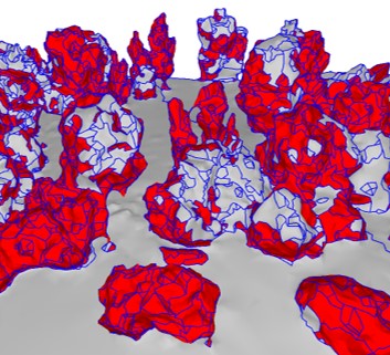
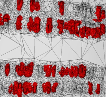
$\lambda^{f}=0.3$	$\lambda^{f}=0.6$	$\epsilon^{(seg)}=30$	$\epsilon^{(seg)}=80$	$\epsilon^{(str)}=20$	$\epsilon^{(str)}=80$
$\lambda^{s}=0.2$	$\lambda^{s}=0.4$	$\epsilon^{(seed)}=15$	$\epsilon^{(seed)}=30$	$\epsilon^{(reg)}=30$	$\epsilon^{(reg)}=60$

Figure 12: Sensitivity analysis of parameters in face (top) and texture annotation (bottom) with the same user interactions.

Mesh	$\sigma^{m}=0.0$	$\sigma^{m}=0.2$	$\sigma^{m}=0.4$
Texture image	$\sigma^{t}=0$	$\sigma^{t}=1$	$\sigma^{t}=3$

Figure 13: Sensitivity analysis of data quality in protrusion extraction (top) and local region extraction (bottom). $\sigma^{m}$ and $\sigma^{t}$ represent the standard deviations of Gaussian noise of different inputs.

5 Summary

We introduced SUM Parts, a part-level semantic segmentation dataset for urban meshes covering $2.5\,\text{km}^{2}$ with 21 classes. A novel annotation tool facilitates the semantic labeling of mesh faces and texture pixels with efficient 2D/3D selection strategies, streamlining the annotation of 3D urban scenes. Our evaluations show that our approach outperforms existing interactive annotation methods.
Applications. Our interactive annotation method can also handle complex indoor scenes, compact building models, and images (see Fig.˜14). The SUM Parts dataset advances lightweight semantic city modeling by providing part-level semantics, enabling automated reconstruction of CityGML LoD3 city models [45, 23].

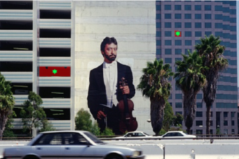
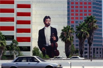
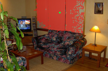
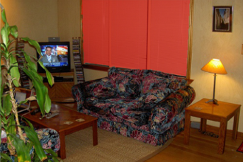
Figure 14: Applications of our annotation tool for indoor meshes (top left), building models (top right), and images (bottom).

Limitations. Our annotation method relies on geometric precision and structural clarity and may be less effective for triangle meshes with topological errors, low resolution, or poor planar over-segmentation. It is also not applicable to natural scenes (e.g., mountains) or complex structures (e.g., palaces) that do not conform to planar and protrusion-based assumptions. In texture annotation, performance can degrade with complex textures, cluttered backgrounds, smaller superpixels (increasing processing time) or larger ones (risking under-segmentation), shadows, or regions with minimal color differentiation.

Supplementary Material

6 Details on annotation tool

6.1 Face-based annotation

Protrusion score.

By measuring the distance and angle from face $f_{i}$ to support plane $P^{f}_{k}$, we define protrusion score $p_{i}=d_{i}+\omega_{i}\cdot\theta_{i},$ where

$$d_{i}=\max_{t\in\{0,1,2\}}\left(\text{dist}(v_{t,i},P^{f}_{k})\right)$$

is the maximum Euclidean distance from the vertices $v_{t}$ of the face $f_{i}$ to the support plane $P^{f}_{k}$. The angle weight $\theta_{i}$ is calculated by measuring the angle $\hat{\theta}_{i}=\cos^{-1}(\mathbf{n}_{i}\cdot\mathbf{n}_{k})$ between the normal $\mathbf{n}_{i}$ of face $f_{i}$ and the normal $\mathbf{n}_{k}$ of support planar segment $P^{f}_{k}$, defined as:

$$\theta_{i}=\frac{\min(\hat{\theta}_{i},180^{\circ}-\hat{\theta}_{i})}{90^{\circ}}.$$

Geometric consistency.

To measure the geometric consistency between adjacent faces, we utilize an interior shrinking ball algorithm derived from the 3D medial axis transform to compute the ball radii for each face [56, 46].

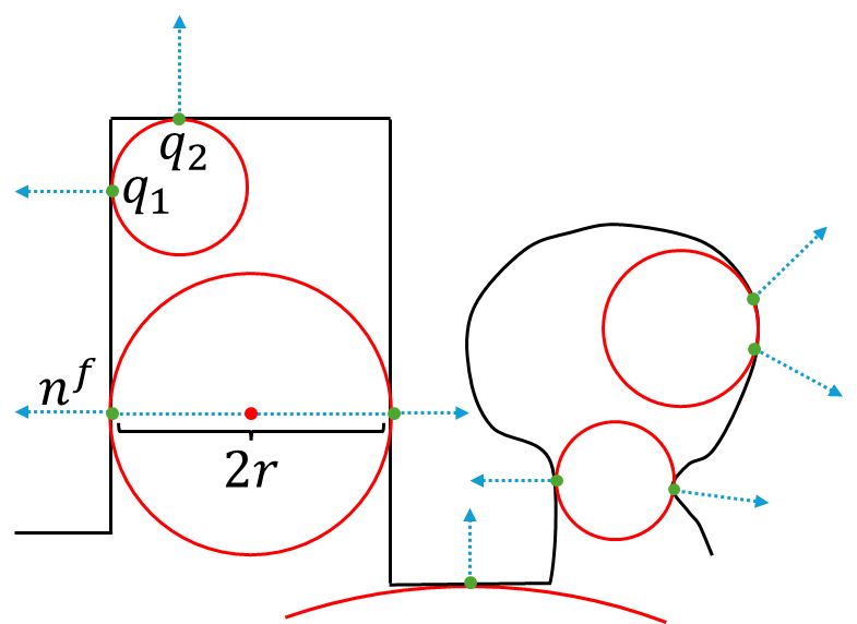
Figure 15: Cross-sectional view of interior shrinking balls (red) in urban scenarios.

In urban mesh scenarios, larger shrinking balls typically correspond to major geometric structures such as the terrain or main surfaces of buildings, whereas smaller balls indicate sharp structures or protrusions (as shown in Fig.˜15). Consequently, the size of these balls can indirectly reflect the local structural scale, suggesting that adjacent faces within the same geometric structure should have similar radii. The mesh shrinking ball radius is derived as

$$r=\frac{\|q_{1}-q_{2}\|^{2}}{2(\mathbf{n}^{f}\cdot(q_{1}-q_{2}))},$$

where $r$ refers to the radius $r_{i}$ or $r_{j}$, and $\mathbf{n}^{f}$ denotes the normal $\mathbf{n}_{i}$ or $\mathbf{n}_{j}$ of the respective faces $f_{i}$ or $f_{j}$; $q_{1}$ and $q_{2}$ are the tangent points on the faces.

Planar segment matching.

We define the feature vector $\mathbf{F^{(seg)}}$ to quantify segment matching similarity, including:

• Geometric homogeneity: Differences in area between geometrically similar segments are calculated as:

  $$\Delta A^{(seg)}=\frac{\left|\text{{area}}^{(c)}-\text{{area}}^{(t)}\right|}{\text{{area}}^{(t)}},$$

  where $\text{{area}}^{(c)}$ and $\text{{area}}^{(t)}$ are the areas of the candidate and template segments, respectively.

• Spatial distribution: Vertical distribution similarity is measured by comparing weighted average heights:

  $$\Delta H^{(seg)}=\left|\frac{\sum_{i=1}^{m^{\prime}}z_{i}\cdot a_{i}}{\text{{area}}^{(c)}}-\frac{\sum_{j=1}^{m^{\prime\prime}}z_{j}\cdot a_{j}}{\text{{area}}^{(t)}}\right|.$$

  where $z_{i}$ and $a_{i}$ denote the z-coordinate and area of each face $f_{i}$ in the candidate segment $P^{(c)}_{k}$. $z_{j}$ and $a_{j}$ denote those in the template segment $P^{(t)}$.

• Spatial orientation: Similarity in vertical orientation is assessed between segments $P^{(c)}_{k}$ and $P^{(t)}$ [51].

• Shape sphericity: Calculated using eigenvalues from triangle vertices of the segment $P^{(c)}_{k}$ and $P^{(t)}$ to evaluate similarity [59].

• Photometric coherence: Color similarity is assessed using CIELAB [38] color distance and greenness [41] difference.

Protrusion matching.

For seed expansion, in addition to spatial and segment scale constraints, we introduce optional topology constraints based on adjacency to optimize user focus and simplify inspection. In urban scenes, small protrusions (e.g., cars, balconies, dormers) reduce global matching efficiency by increasing inspection workload and computation (e.g., matching cars globally takes 5s, whereas planar facades take only 0.4s, see Fig.˜4(b)). Therefore, we set topology constraints as the default for practical efficiency by confining the search space to planar segments of the template support surface (e.g., limiting annotations to the current facade for facade installations).

The feature vector $\mathbf{F^{(str)}}$ includes:

• Spatial compactness: The compactness of a protrusion is quantified by considering its volume. We expect similar protrusions to have comparable values, defined as

  $$\Delta V^{(str)}=\left|\frac{\text{{vol}}^{(c)}}{\text{{vol}}^{(c)}_{box}}-\frac{\text{{vol}}^{(t)}}{\text{{vol}}^{(t)}_{box}}\right|,$$

  where $\text{{vol}}^{(c)}$ and $\text{{vol}}^{(c)}_{box}$ represent the volume of $f^{(c)}$ and its bounding box volume, respectively. $\text{{vol}}^{(t)}$ and $\text{{vol}}^{(t)}_{box}$ are the corresponding values for $f^{(t)}$.

• Surface complexity: We assume complex 3D shapes decompose into multiple planar segments. Surface complexity similarity is measured by the ratio of the number of planar segments in the template and candidate protrusions, defined as

  $$\Delta N^{(str)}=\left(\frac{\max(n^{(t)},n^{(c)})}{\min(n^{(t)},n^{(c)})}\right)^{\mu},$$

  where $n^{(t)}$ and $n^{(c)}$ respectively represent the number of planar segments for the template and candidate protrusions, and $\mu={\min(n^{(t)},n^{(c)})}$.

• Structural features: Measuring the similarity of protrusions involves comparing their structural features through eigenvalue analysis including linearity, planarity, and sphericity [59]. We determine similarity by the $\ell_{1}$ distance in the feature space, including differences in linearity $\Delta L^{(str)}$, planarity $\Delta P^{(str)}$, and sphericity $\Delta S^{(str)}$.

6.2 Texture-based annotation

Gaussian mixture model (GMM).

$G_{k}$ denotes the GMM for the $k$-th channel, defined as

$$G_{k}(S)=\sum_{m=1}^{M}\pi_{km}\mathcal{N}(x;\mu_{km},\Sigma_{km}),$$

where $S$ represents the superpixel $S_{0}$ or $S_{j}$. $x$ is a pixel sample point of $S$, and $M$ is the number of components in GMM ($M$ set to 5 in all experiments in this paper). $\mathcal{N}(s;\mu,\Sigma)$ denotes the multivariate normal distribution, with $\mu$ representing the mean for superpixels $S_{0}$ or $S_{j}$, and $\Sigma$ denotes their respective covariance matrices.

Local color consistency.

For local color consistency, where $\rho_{j}=\Delta E_{00}(U_{0},U_{j})$ is the color distance (i.e., CIEDE2000 [38]) from the superpixel $S_{j}$ to its seed $S_{0}$. To more accurately capture the intrinsic structure and variability within superpixels’ color distributions, we employ a GMM to compute the average Lab color, represented by $U=\sum_{m=1}^{M}\pi_{m}\mu_{m}$, where $U$ represents $U_{0}$ or $U_{j}$, with $\pi_{m}$ as the mixing weight and $\mu_{m}$ as the mean for the $m$-th Gaussian component in the Lab color space. Additionally, seed samples for $U_{0}$ are taken from its first-order neighborhood, whereas samples for $U_{j}$ come from its own pixels.

Region-based template matching.

The feature vector $\mathbf{F^{(reg)}}$ includes:

• Shape index: To assess shape similarity, we use a shape index reflecting elongation or flatness, which is defined as: $r=\frac{\min(w,h)}{\max(w,h)},$ where $w$ and $h$ represent the width and height of the object’s bounding box, respectively. The similarity between regions is calculated as: $\Delta I^{(reg)}=|r_{c}-r_{t}|,$ where $r$ represents the ratio $r_{c}$ of the candidate region or $r_{t}$ of the template region.

• Shape regularity: We assess shape regularity to calculate the similarity between areas. Similar to structural matching, compactness is used to describe how well a shape fills its bounding box, defined as:

  $$\Delta A^{(reg)}=\left|\frac{\text{{area}}^{(c)}}{\text{{area}}^{(c)}_{box}}-\frac{\text{{area}}^{(t)}}{\text{{area}}^{(t)}_{box}}\right|,$$

  where $\text{{area}}^{(c)}$ and $\text{{area}}^{(t)}$ represent the area of the candidate and template regions, respectively, and $\text{{area}}^{(c)}_{box}$ and $\text{{area}}^{(t)}_{box}$ are the areas of their bounding boxes.

• Contextual features: Similar regions should have similar internal and external color distributions. We evaluate these differences using the Wasserstein distance, calculated as: $\Delta D^{(reg)}=\left|W(G_{k}(R^{(c)}_{in}),G_{k}(R^{(c)}_{out}))-W(G_{k}(R^{(t)}_{in}),G_{k}(R^{(t)}_{out}))\right|,$ where $R^{(c)}_{in}$ and $R^{(c)}_{out}$ denote the interior and exterior pixel collections of the candidate region, respectively, and $R^{(t)}_{in}$ and $R^{(t)}_{out}$ for the template region. The external region $R_{out}$ includes pixels covered but not selected during local expansion.

Scalability.

Our workflow is fully compatible with deep learning-based frameworks like Semantic-SAM [33] and Mask DINO [32]. Combining them demonstrates the potential to accelerate template generation through prompt-based segmentation at various granularities and refine template matching with instance/object detection. Additionally, our 2D paint canvas (see Fig.˜5) converts texture segments into images that are compatible with these segmentation methods. This, combined with our annotated dataset, allows direct training on 3D textured surfaces, setting the stage for future improvements in efficiency and accuracy.

7 Details on benchmark results

7.1 Evaluation of interactive annotation

Evaluation metrics.

Traditional metrics, such as click counts to achieve specific Intersection over Union (IoU) or Average Precision (AP), are quantifiable but do not fully capture the true efficiency of the annotation process. The main shortcomings of these methods include:

• Evaluation limitations: Relying solely on IoU or AP does not fully capture annotation comprehensiveness. For example, a 90% IoU may still require multiple boundary adjustments for accuracy.

• Interaction limitations: Click-based interactions alone cannot perfectly annotate boundaries, often requiring tools like lassos or polygons. Additionally, standardized click positions do not account for individual user variations, hindering realistic efficiency assessment.

• Efficiency limitations: Average click counts do not reflect actual interaction efficiency due to varying user speeds. Measuring total annotation time provides a more accurate assessment of efficiency.

To address these issues, we developed an evaluation system comprising Intersection over Union (IoU), Boundary IoU (BIoU), number of operations (Oper), annotation time (Time), and smart interaction ratio (SR). BIoU assesses boundary annotation accuracy [13, 20]. Oper counts mouse clicks and keyboard keystrokes. Time measures annotation duration in seconds. SR quantifies the frequency of non-manual interactions (counting only click-based selections, excluding other operations). Our evaluation is based on user studies with $u$ users across $n$ test scenes, each with $c$ categories. The average metrics are calculated as follows:

• Evaluating a single scenario. For a given scenario $s$, annotated by $u$ users across $c$ categories, $\overline{mIoU}$, $\overline{mBIoU}$, $\overline{mOper}$, $\overline{mTime}$, and $\overline{mSR}$, can be obtained by averaging the $IoU$, $mBIoU$, $mOper$, $mTime$, and $mSR$ values across all users and categories.

• Evaluating multiple scenarios. To obtain $\overline{M}$, $\overline{B}$, $\overline{O}$, $\overline{T}$, and $\overline{S}$, the averages of for multiple scenarios, we take the average of each scenario’s $\overline{mIoU}$, $\overline{mBIoU}$, $\overline{mOper}$, $\overline{mTime}$, $\overline{mSR}$ and then average these values:

  $$\overline{M} =\frac{1}{n}\sum_{s=1}^{n}\overline{mIoU}_{s} \overline{B} =\frac{1}{n}\sum_{s=1}^{n}\overline{mBIoU}_{s}$$

  $$\overline{O} =\frac{1}{n}\sum_{s=1}^{n}\overline{mOper}_{s} \overline{T} =\frac{1}{n}\sum_{s=1}^{n}\overline{mTime}_{s}$$

  $$\overline{S} =\frac{1}{n}\sum_{s=1}^{n}\overline{mSR}_{s}$$

In the user study, we recorded each user’s annotation progress and interactions in real-time, requiring at least 95% scene completion based on mesh area or texture pixels.

Comparisons.

Tab.˜5 shows that our method outperforms segment-based annotation [19] in object region and boundary quality. Across all four test scenarios, it significantly reduces both interaction counts and annotation time. We also provide additional qualitative analysis, as shown in Fig.˜16 and Fig.˜17.

Metric	Method	Cour.	Stre.	Park.	Harb.
$\overline{mIoU}_{s}(\%)$	Seg	89.1	94.0	92.1	91.1
	Ours	89.5	94.2	92.9	92.2
$\overline{mBIoU}_{s}(\%)$	Seg.	72.7	85.4	70.6	70.3
	Ours.	72.4	84.5	71.9	71.0
$\overline{mOper}_{s}$	Man.	18154	1589	3559	3714
	Seg.	17645	1407	2529	2894
	Ours	13231	909	1797	1957
$\overline{mTime}_{s}(s)$	Man.	11401.0	969.5	2146.5	2215.8
	Seg.	10441.3	757.0	1441.4	1623.7
	Ours	9107.2	498.0	1105.9	1257.5
$\overline{mSR}_{s}(\%)$	Ours	66.5	94.9	85.8	84.8

Table 5: Performance evaluation of interactive mesh face annotation methods across four scenarios: Cour. (courtyard complex), Stre. (streets with vehicles), Park. (park with trees), Harb. (harbor with ships). Methods include Man. [52] and Seg. [19]. Highest values are shown in bold.

From Tab.˜6, our method has slightly lower $\overline{M}$ than GrabCut [50], but achieves higher $\overline{mIoU}_{s}$ in most scenarios and excels in boundary quality. While SimpleClick [37] is more efficient in interaction count, our method outperforms others in most scenarios. Though slower than SAM [27], our method still surpasses other methods in interaction time. The need for manual corrections enhances annotation quality without significant time cost, and our approach delivers more accurate boundaries with similar correction workloads compared to deep learning methods. We achieve this through: (1) Better quality from the user-defined template that enables pixel-level boundary control, outperforming deep learning-based clicks by approximately +3.5$\sim$6.5% mIoU and +18.4$\sim$19.5% boundary mIoU ( Tab.˜4), especially for regular shapes like windows in Fig.˜11. (2) Higher efficiency offered by reusable, scale- and rotation-invariant templates, which reduces the interaction count by -18.7% compared to SAM (582 vs. SAM’s 716) and annotation time by -23% compared to SimpleClick (663.3s vs. SimpleClick’s 861.3s), benefiting repetitive structures ( Tab.˜4). Although SAM is slightly faster and SimpleClick requires fewer interactions, our intentional design using handcrafted templates instead of intensive smart clicks prioritizes higher-quality annotations while maintaining a similar total annotation time.

Metric	Method	Fac1.	Fac2.	Par1.	Par2.	Rod1.	Rod2.
$\overline{mIoU}_{s}(\%)$	Gra.	80.2	87.3	94.0	90.4	91.3∗	85.4
	SAM	81.0	86.4	85.3	86.4	86.5	80.7
	Sip.	73.7	77.5	87.9	86.2	84.0	79.1
	Ours	79.2	88.7	95.0	91.2	91.3	82.1
$\overline{mBIoU}_{s}(\%)$	Gra.	27.8	45.4	63.7	45.8	49.9	50.1
	SAM	24.7	33.9	25.8	23.3	34.1	37.0
	Sip.	19.7	26.8	38.0	34.4	31.8	34.6
	Ours	28.1	50.5	67.8	48.6	50.5	50.6
$\overline{mOper}_{s}$	Man.	515	124	497	297	718	1764
	Gra.	717	156	462	243	960	1729
	SAM	715	319	363	319	1020	1684
	Sip.	297	119	77	78	400	539
	Ours	487	105	497	213	720	1468
$\overline{mTime}_{s}(s)$	Man.	816.9	185.6	636.7	280.1	801.7	1941.4
	Gra.	920.1	242.6	494.9	270.8	836.3	1920.6
	SAM	565.5	150.6	460.9	389.5	800.6	1476.5
	Sip.	1128.5	338.9	197.7	230.8	1526.4	1745.5
	Ours	631.1	155.8	565.9	189.1	767.9	1670.3
$\overline{mSR}_{s}(\%)$	Gra.	7.1	11.8	59.3	66.5	9.9	26.7
	SAM	94.7	92.8	78.8	78.6	49.2	36.0
	Ours	20.3	21.2	51.6	75.8	32.2	40.8

Table 6: Performance evaluation of interactive texture annotation methods across six scenarios: Man. (manual), Gra. (GrabCut [50]), SAM (Segment Anything [27]), Sip. (SimpleClick [37]), Fac1./Fac2. (facades 1 & 2), Par1./Par2. (parks 1 & 2), Rod1./Rod2. (roads 1 & 2). ^∗GrabCut on Rod1. achieved 91.29%, slightly below our method’s 91.31%. Highest values are in bold.

For regular-shaped objects, interactive clicking is suboptimal. As shown in Fig.˜18 and Fig.˜19, single clicks lack boundary precision, and multiple clicks do not significantly improve accuracy. Repetitive structures increase the annotation burden due to frequent clicking. Instead, users achieve high precision by drawing rectangles or polygons for elements like windows or doors. Our method enables efficient annotation of similar structures by creating a graphical template once. In summary, if manual corrections in semi-automatic annotations take as much or more time than fully manual annotations, the method loses its utility. Additional qualitative results from our annotation methods are presented in Fig.˜20.

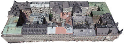
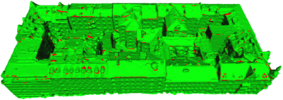
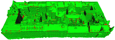
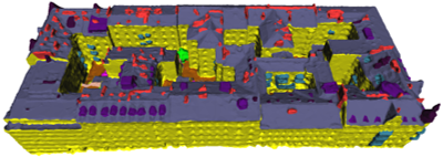
Input	Segment-based (errors) [19]	Ours (errors)	Manual [52]

Figure 16: Qualitative analysis of interactive mesh face annotations and their error maps (shown in red) for the courtyard complex.

Input	Segment-based (errors) [19]	Ours (errors)	Manual [52]

Figure 17: Qualitative analysis of interactive mesh face annotations and their error maps (shown in red) for the street with vehicles.

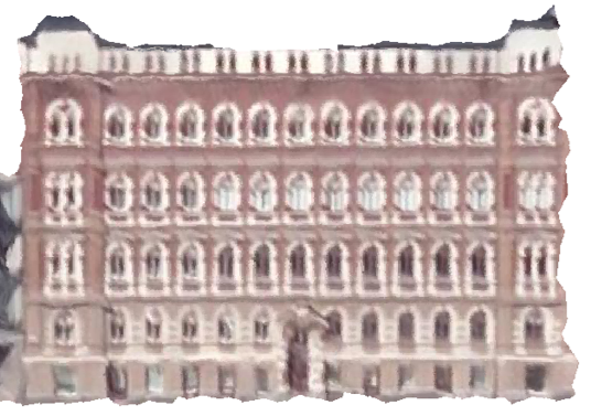
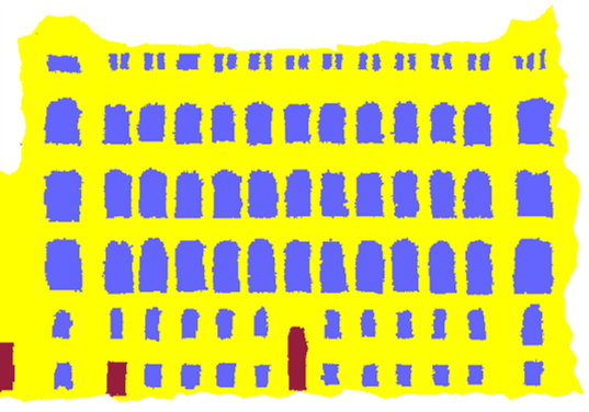
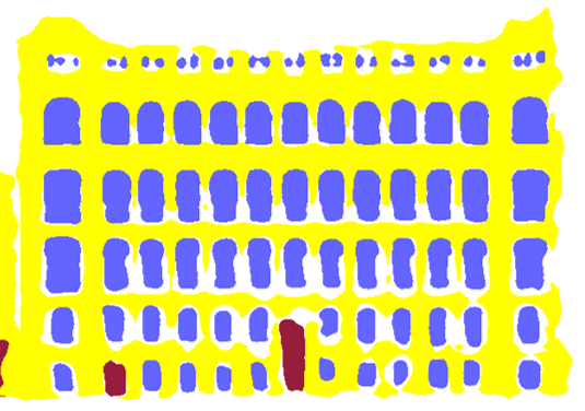
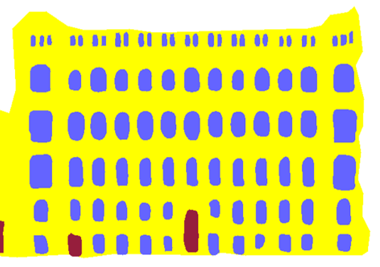
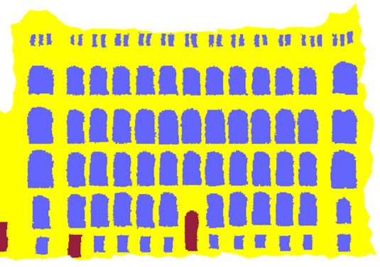
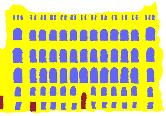
Input	GrabCut [50]	Simclick [37]	SAM [27]	Ours	Manual

Figure 18: Qualitative analysis of interactive texture annotation results for the facade.

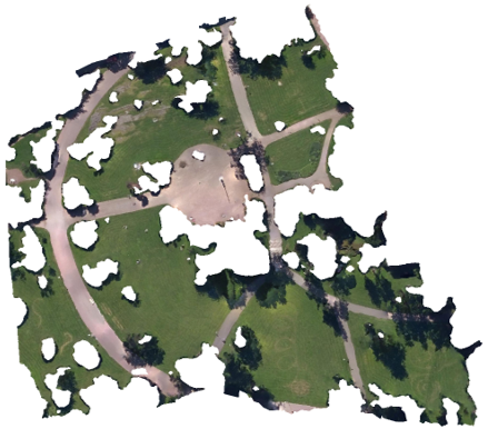
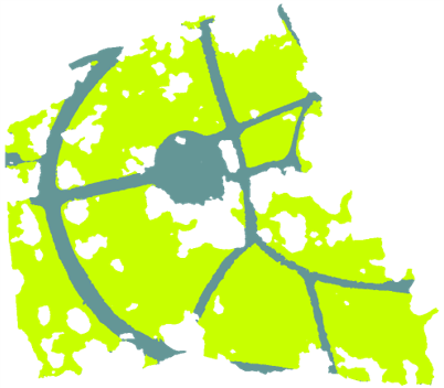
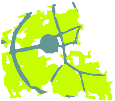
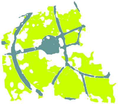
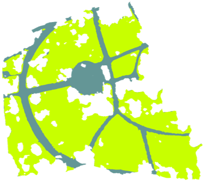
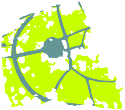
Input	GrabCut [50]	Simclick [37]	SAM [27]	Ours	Manual

Figure 19: Qualitative analysis of interactive texture annotation results for the park.

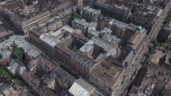
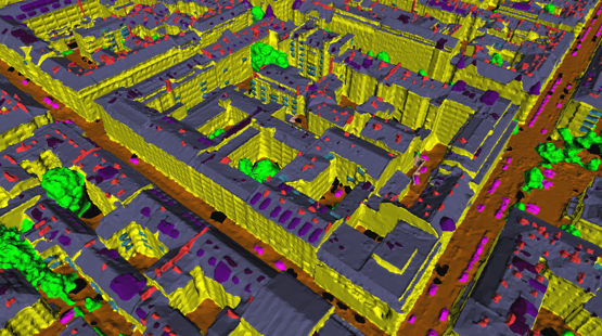
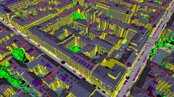
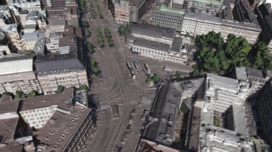
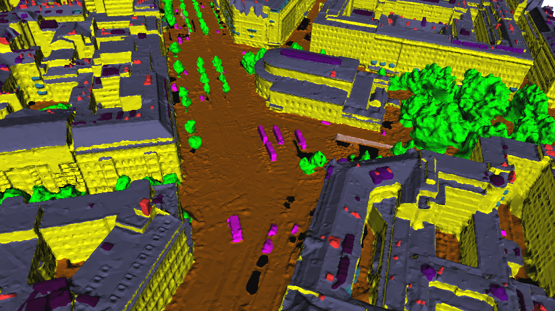
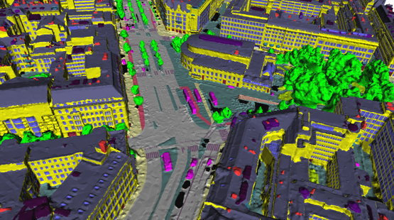
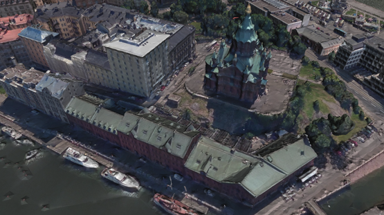
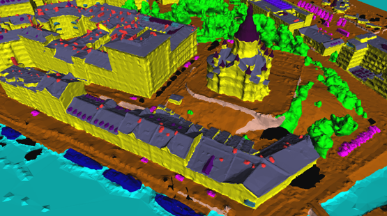
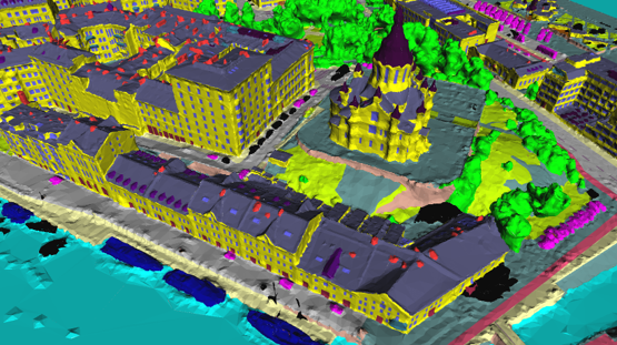
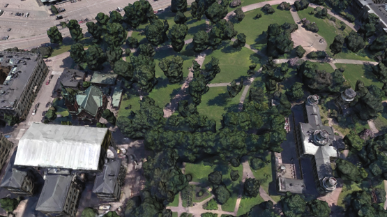
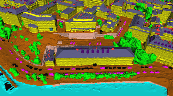
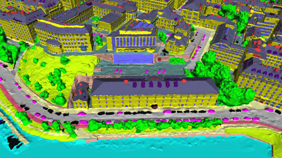
Input	Face-based annotation	Texture-based annotation

Figure 20: Examples of part-level annotated semantic urban meshes are displayed from the first to the third column, showing textured meshes, face-based semantic meshes (13 classes), and texture-based semantic meshes (19 classes), respectively.

Ablation studies on template matching.

Our feature design is grounded in geometric priors (shape properties and structural distribution), label-free operation, and computational efficiency, validated through hierarchical ablation studies (mIoU) as follows. For matching: (1) Planar segments (e.g., roofs, best 88.4% in Fig.˜16). Removing geometric homogeneity (-6.1%), spatial distribution (-13.8%), orientation (-13.3%), and shape sphericity (-1.8%) caused performance drops. (2) Protrusions (e.g., cars, best 97.0% in Fig.˜17). When spatial compactness (-2.6%), surface complexity (-1.2%), and structural features (-1.6%) were removed, precise matching suffered significantly. (3) Regions (e.g., windows, best 90.7% in Fig.˜18). Eliminating shape index (-5.2%), regularity (-38.1%), and contextual features (-20.3%) severely impaired boundary alignment and color consistency. These results highlight the essential role of each feature and their combined effectiveness, confirming our method’s superior performance.

7.2 Evaluation of semantic segmentation

1) Face labeling track.  Tab.˜7 provides a detailed comparison of results for all face-labeled classes. Due to class imbalance, most methods show better performance in categories with more samples and poorer performance in categories with fewer samples. We conducted qualitative analyses on all methods except PointNet for two scenarios, as shown in Fig.˜21 and Fig.˜22.

2) Pixel labeling track. Tab.˜8 provides a detailed comparison of results for all face-labeled and pixel-labeled classes. PointVector [17] surpasses other methods in all categories, particularly with pixel labels. However, compared to the categories shared with Tab.˜7, the IoU results for most methods have decreased. This is mainly because the three mesh sampling methods produce relatively uniform point clouds, failing to capture the geometric density variations inherent in adaptive meshes. Additionally, the increase in the number of classes has exacerbated the issue of class imbalance. We performed qualitative analyses for all methods in two scenarios, with global and zoomed-in views, as shown in Fig.˜23 and Fig.˜24.

	terr.	hveg.	faca.	wate.	car	boat	roof.	chim.	dorm.	balc.	roin.	wall	OA	mAcc	mIoU
RF_MRF	81.6	86.6	81.3	84.5	24.8	3.7	73.3	27.6	0.0	4.8	0.4	5.9	85.2	45.3	39.5
SUM_RF	84.8	88.1	84.0	79.0	42.5	10.6	77.7	42.4	3.5	22.2	4.7	12.7	86.9	53.6	46.0
PSSNet	80.7	90.5	85.2	64.2	52.6	13.0	78.1	44.0	6.6	25.7	6.9	16.6	86.3	56.4	47.0
PoinNetSp.	52.6	7.1	38.6	59.9	0.0	0.0	22.8	0.0	0.0	0.0	0.0	0.0	50.6	22.0	15.1
PoinNet++Sp.	67.9	68.7	59.2	86.1	24.2	11.1	51.1	24.9	0.0	0.0	3.3	1.1	69.0	46.9	33.1
SPGSp.	53.4	55.3	62.5	40.5	27.4	13.1	64.3	33.9	5.1	11.3	3.9	9.9	64.9	55.0	31.7
SparseUNetFc.	88.6	91.7	88.6	76.7	75.6	14.6	82.3	70.1	27.0	49.0	28.0	33.9	90.3	71.7	60.5
Randla-netFc.	86.7	92.3	81.6	87.1	82.9	41.2	71.6	55.6	21.6	27.6	19.0	21.1	86.7	76.3	57.4
KPConvFc.	86.9	90.8	88.3	81.5	66.4	16.5	81.9	66.7	16.1	45.3	21.2	28.2	90.1	64.7	57.5
PointNextFc.	91.0	95.0	90.4	81.6	91.2	17.9	83.1	74.6	33.8	56.0	30.0	39.3	91.8	77.2	65.3
PointTransV3Fc.	88.6	90.1	87.9	78.9	72.1	16.1	81.0	66.2	21.4	45.2	25.0	36.4	89.9	70.2	59.1
PointVectorFc.	92.3	96.8	91.7	85.1	95.2	22.0	85.9	82.6	47.9	62.4	38.6	40.0	93.1	80.7	70.0

Table 7: Comparison of 3D semantic segmentation methods for face labeling using optimal sampling. Semantic categories: ‘terr.’ (terrain), ‘hveg.’ (high vegetation), ‘faca.’ (facade), ‘wate.’ (water), ‘roof.’, ‘chim.’ (chimney), ‘dorm.’ (dormer), ‘balc.’ (balcony), and ‘roin.’ (roof installation). ^Fc. and ^Sp. denote face-centered and superpixel sampling, respectively. Results are presented as IoU (%), Overall Accuracy (OA %), mean Accuracy (mAcc %), and mean IoU (mIoU %). Highest values in IoU, OA, mAcc, and mIoU are highlighted in bold.

	hveg.	faca.	wate.	car	boa.	roof.	chim.	dorm.	balc.	roin.	wall	wind.	door	lveg.	impe.	road	roma.	cycl.	side.	OA	mAcc	mIoU
PoinNetSp.	0.5	13.3	16.5	0.0	2.1	7.9	0.0	0.0	0.0	0.0	0.0	0.0	0.0	0.0	8.5	0.0	0.0	0.0	0.2	17.3	9.8	2.6
PoinNet++Sp.	72.7	47.5	86.4	34.9	12.4	52.4	28.1	0.0	5.3	5.6	0.4	13.0	5.0	42.4	31.2	14.6	9.5	0.0	7.3	55.4	35.2	24.7
SPGSp.	58.2	50.8	18.4	24.1	2.7	60.4	39.9	3.1	13.6	4.4	10.5	2.4	4.0	13.4	14.6	31.0	0.0	1.7	12.1	51.5	34.5	19.2
SparseUNetRd.	88.8	70.0	5.9	51.6	2.5	79.8	55.0	12.3	45.4	22.6	31.5	32.0	12.3	15.2	43.8	44.6	5.2	0.6	35.8	72.9	45.1	34.5
Randla-netSp.	90.5	60.9	84.6	67.6	22.7	74.7	53.3	0.6	29.3	16.2	26.3	33.4	12.8	59.8	48.8	50.2	31.5	0.0	37.1	73.5	57.7	42.1
KPConvSp.	84.0	68.5	81.7	68.6	21.8	78.2	66.4	25.0	41.8	29.6	31.5∗	36.1	14.9	21.4	35.8	50.0	7.3	13.4	34.1	74.4	58.3	42.6
PointNextPo.	90.1	66.2	87.9	68.1	16.3	74.5	59.7	14.9	35.6	19.1	31.0	33.2	13.7	55.5	51.4	55.5	29.0	6.9	40.0	76.0	57.6	44.7
PointTransV3Rd.	85.9	59.9	74.6	64.7	17.8	75.9	58.7	15.3	37.2	16.2	29.3	11.8	7.9	27.1	43.3	51.5	3.5	7.2	33.4	70.6	54.1	38.0
PointVectorSp.	92.7	66.6	92.0	70.2	19.8	76.8	60.8	21.8	37.0	20.6	30.8	37.1	16.5	59.8	53.9	57.4	35.0	16.4	45.0	77.0	63.8	47.9

Table 8: Comparison of 3D semantic segmentation methods for pixel labeling using optimal sampling strategies: ‘hveg.’ (high vegetation), ‘faca.’ (facade surface), ‘wate.’ (water), ‘roof.’ (roof surface), ‘chim.’ (chimney), ‘dorm.’ (dormer), ‘balc.’ (balcony), ‘roin.’ (roof installation), ‘wind.’ (window), ‘lveg.’ (low vegetation), ‘impe.’ (impervious surfaces), ‘roma.’ (road marking), ‘cycl.’ (cycle lane), and ‘side.’ (sidewalk). Additionally, ^Sp. denotes superpixel sampling, ^Rd. for random sampling, and ^Po. for Poisson-disk sampling [14]. Results are presented as IoU (%), Overall Accuracy (OA %), mean Accuracy (mAcc %), and mean IoU (mIoU %). ^∗KPConv’s IoU for wall is 31.46%, slightly below SparseUnet’s 31.47%. Highest values in IoU, OA, mAcc, and mIoU are highlighted in bold.

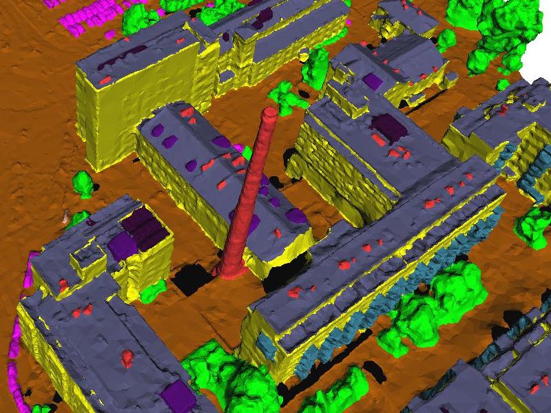
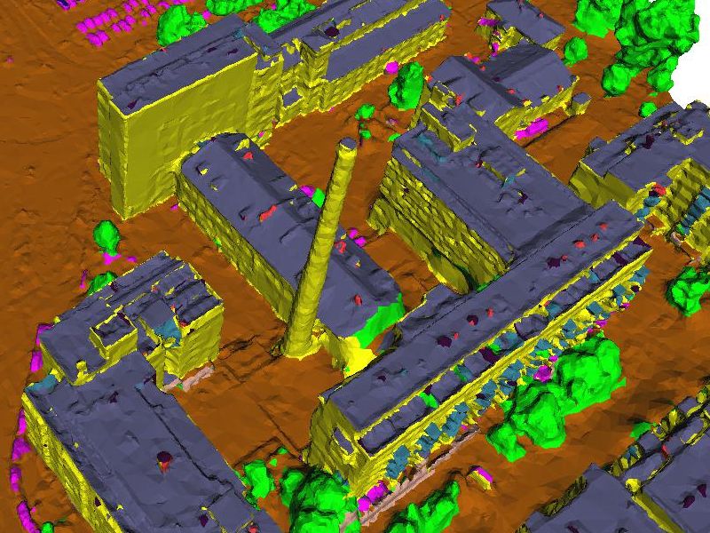
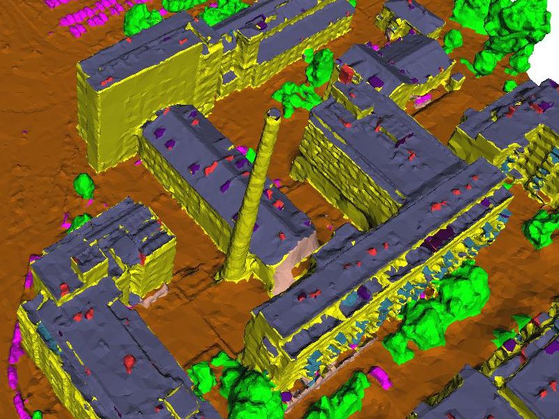
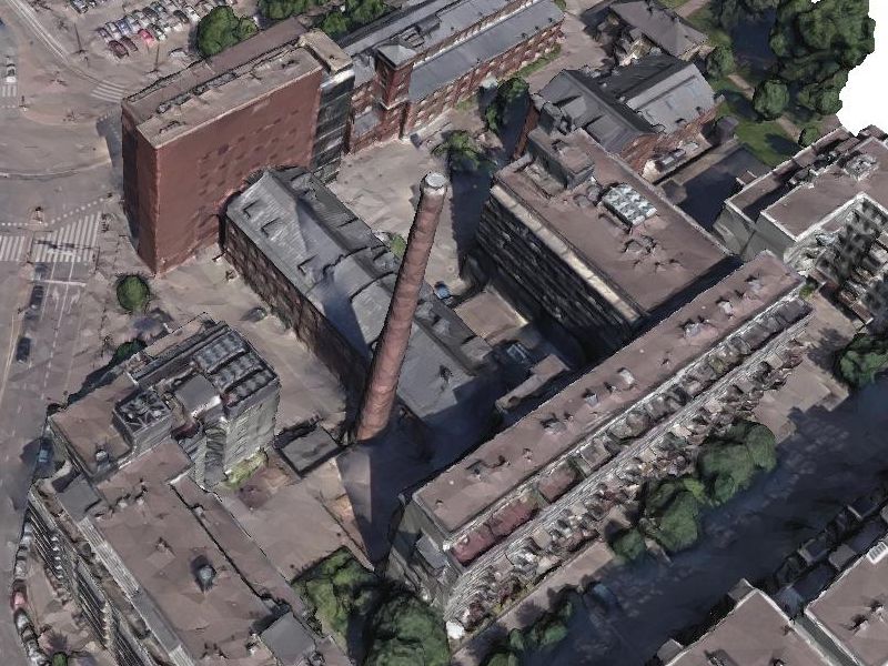
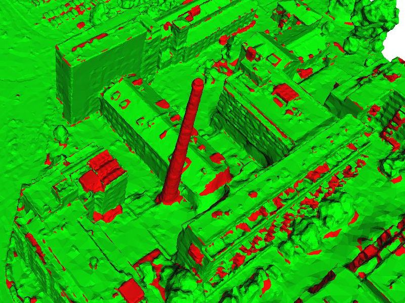
Truth (top), Mesh (bottom)	RF_MRF	SUM_RF	PSSNet
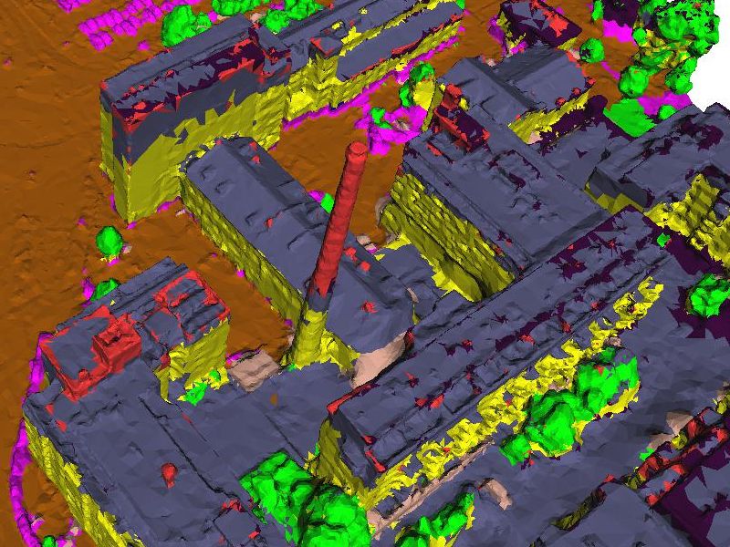
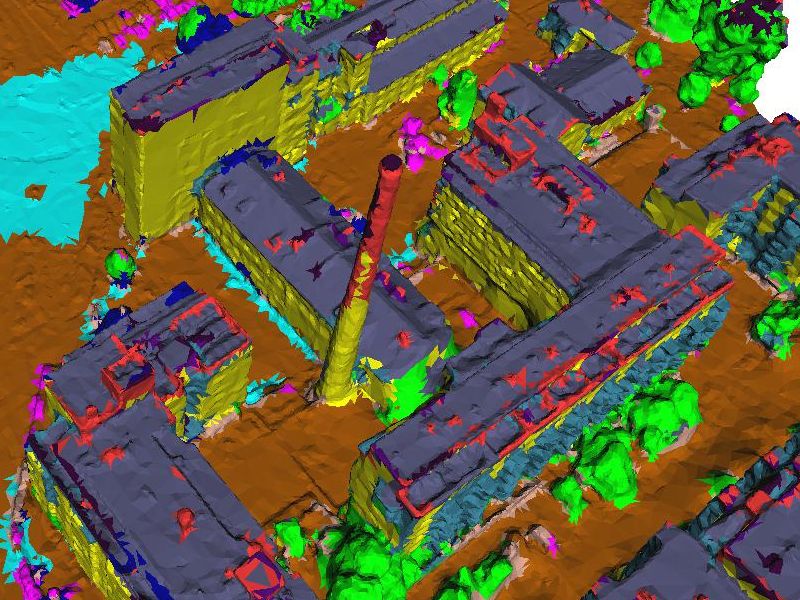
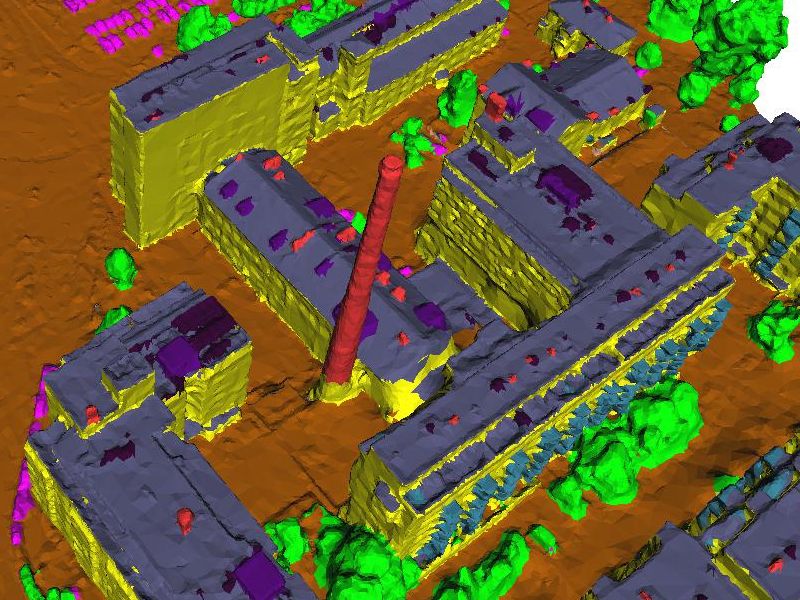
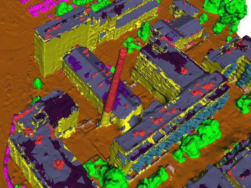
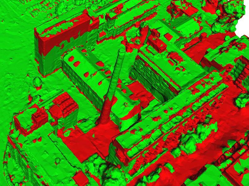
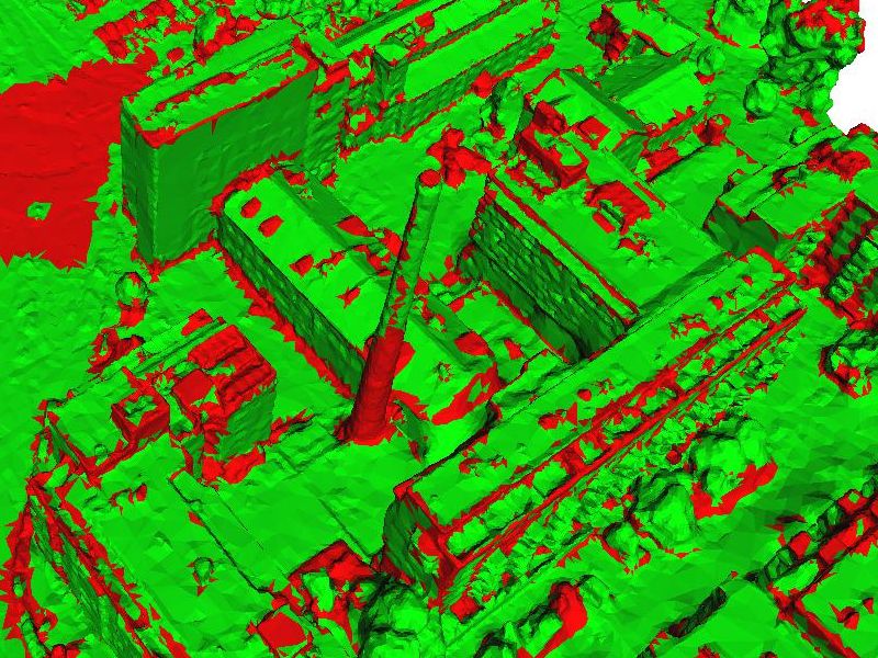
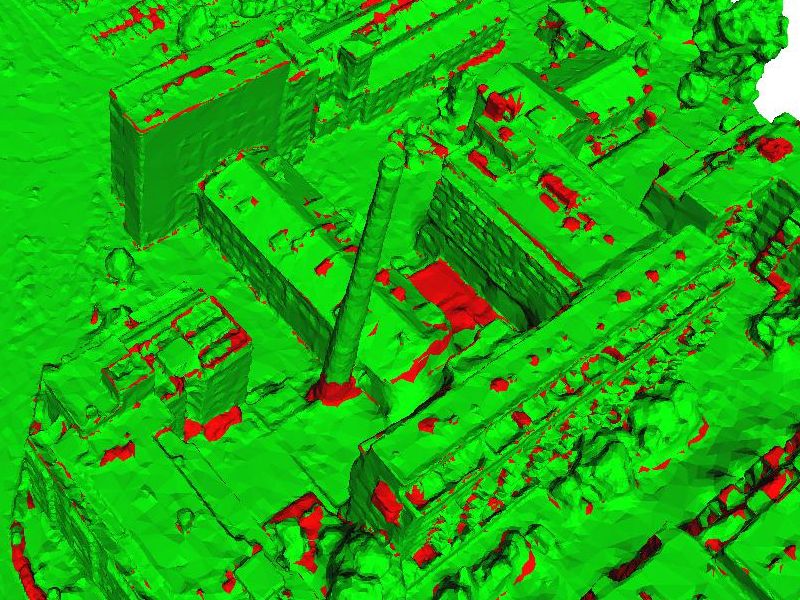
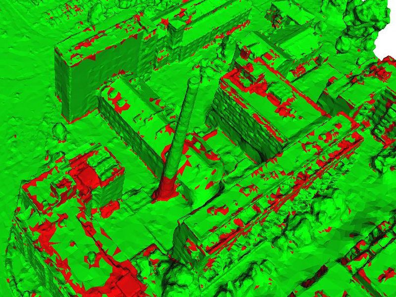
PointNet++Sp.	SPGSp.	SparseUNetFc.	Randla-netFc.
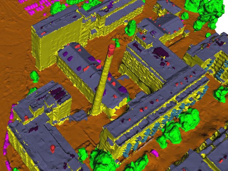
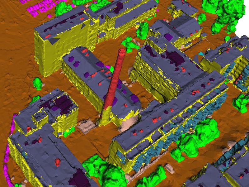
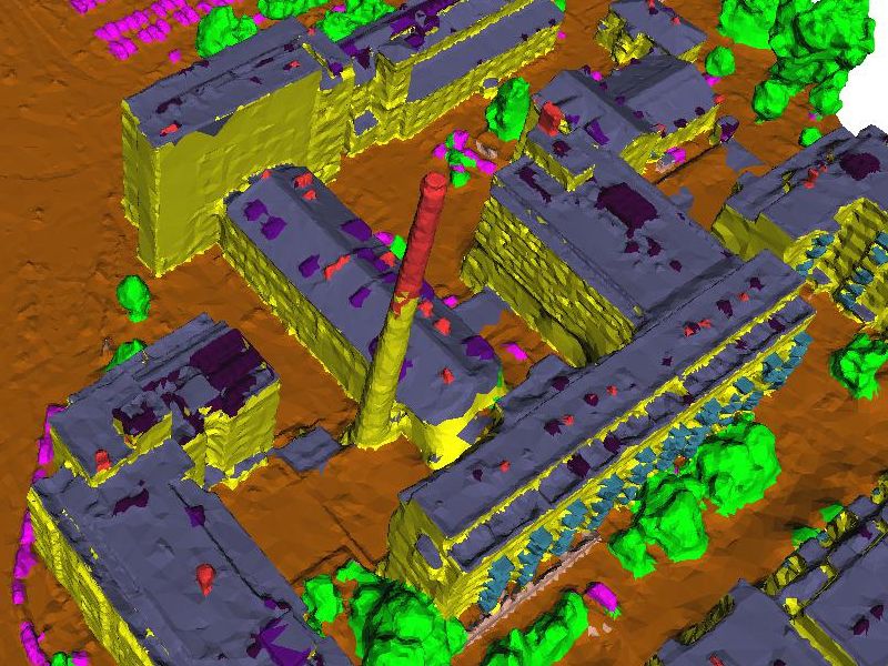
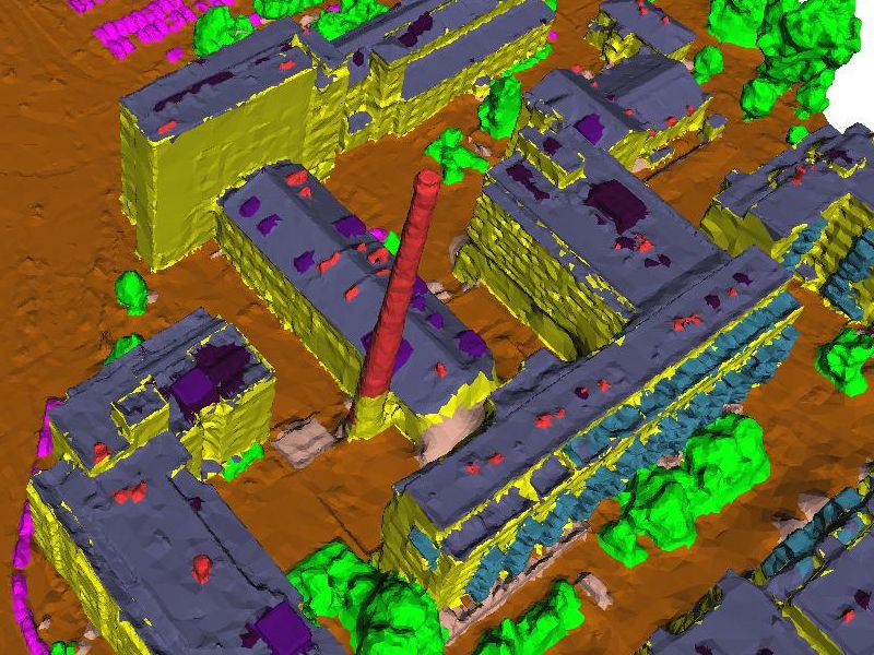
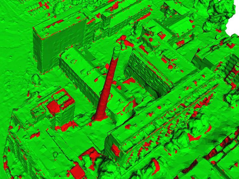
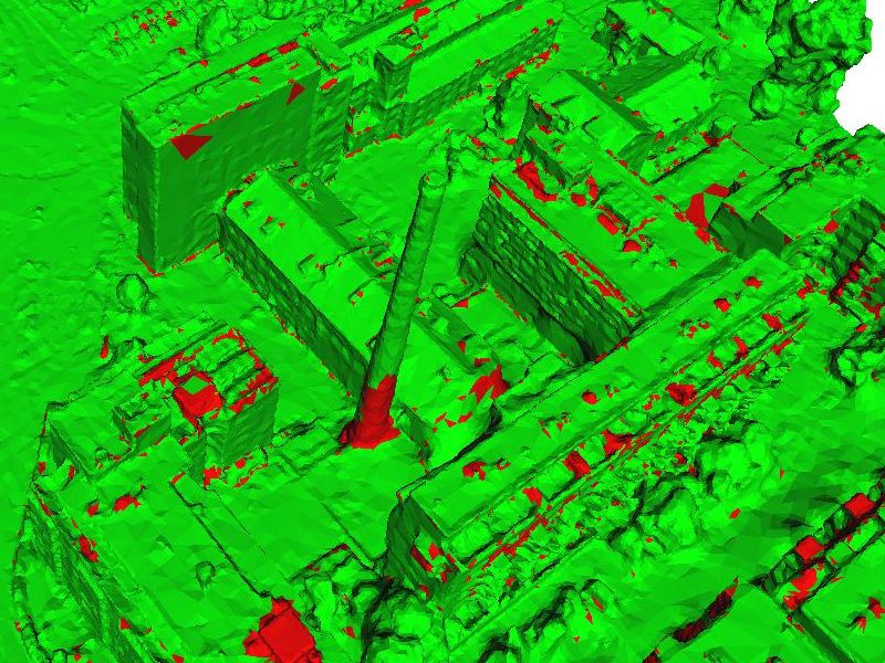
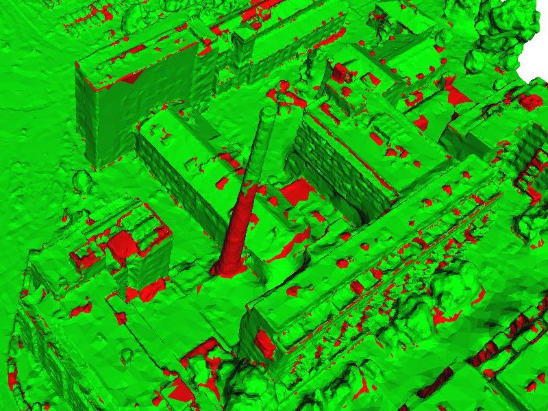
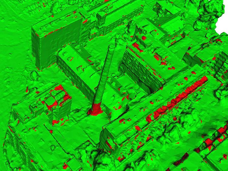
KPConvFc.	PointNextFc.	PointTransV3Fc.	PointVectorFc.

Figure 21: Qualitative analysis of semantic segmentation and error maps in the face labeling track for all methods except PointNet [12] in the first scenario. ^Fc. and ^Sp. denote face-centered and superpixel sampling, respectively.

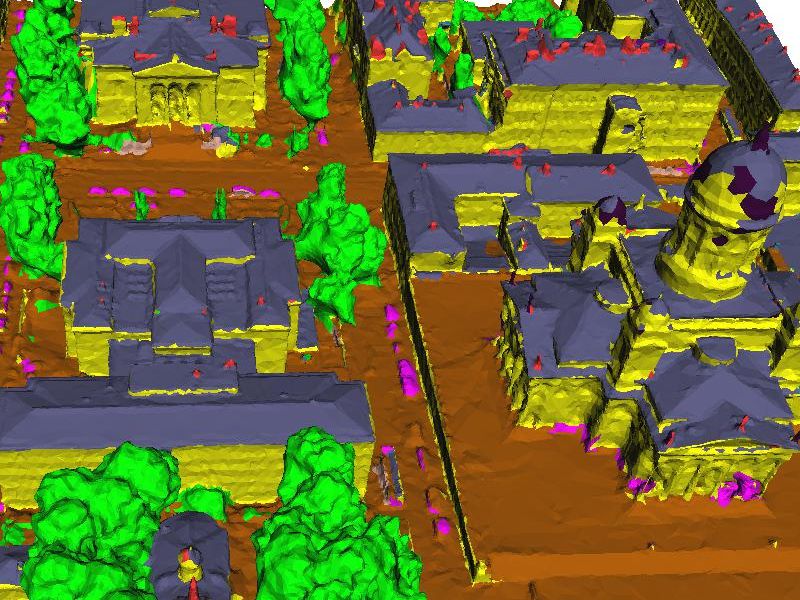
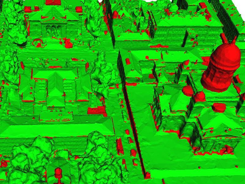
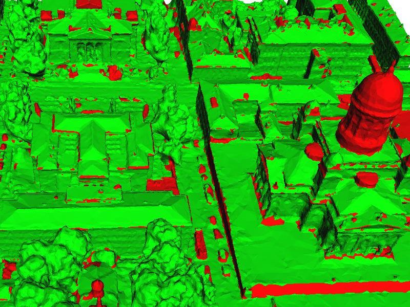
Truth (top), Mesh (bottom)	RF_MRF	SUM_RF	PSSNet
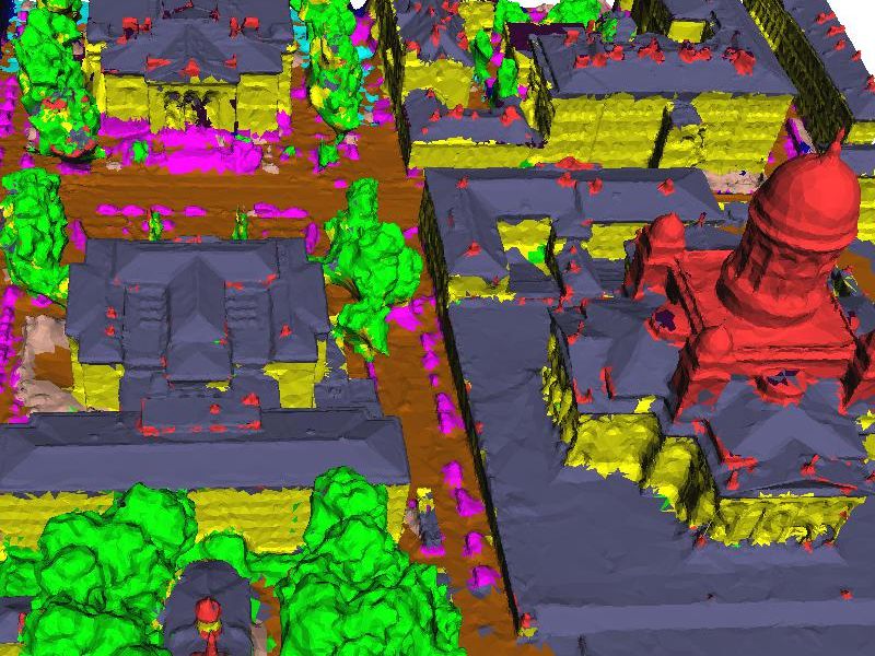
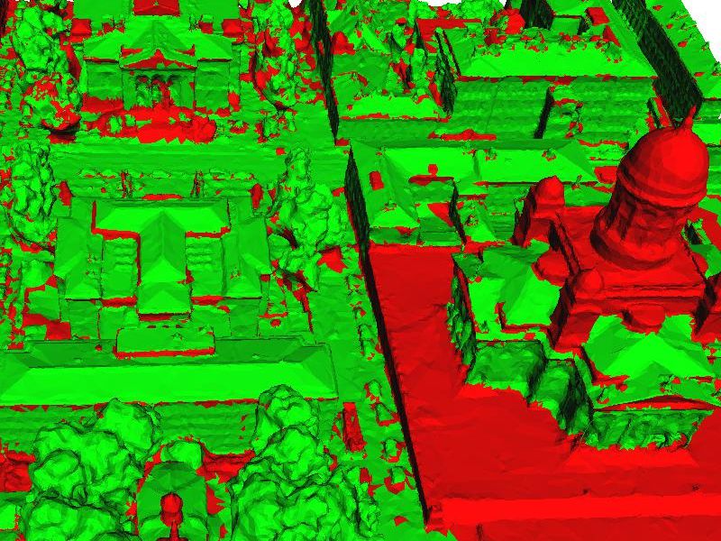
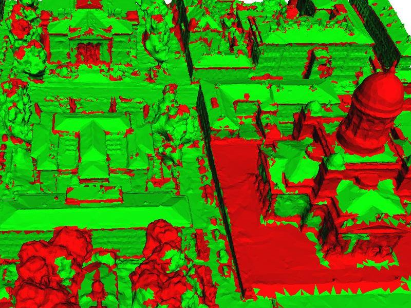
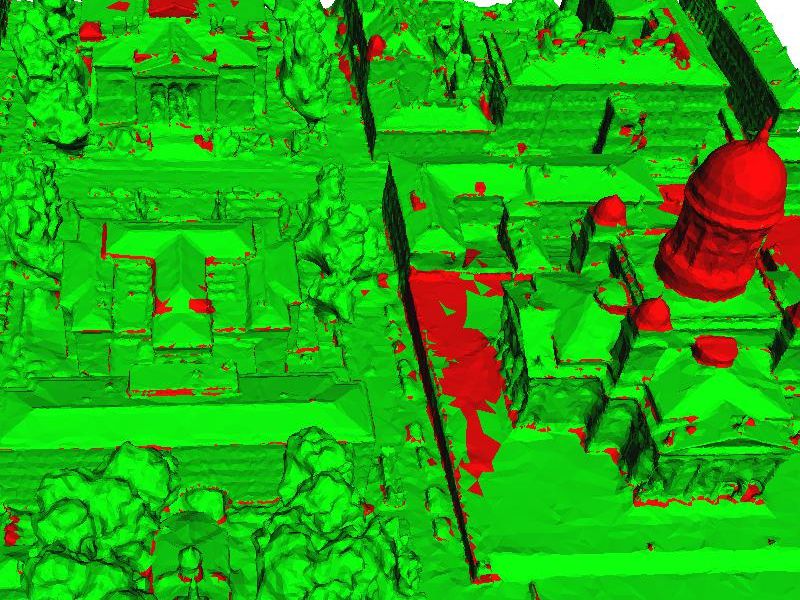
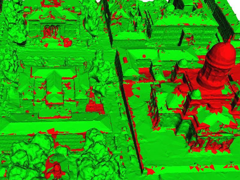
PointNet++Sp.	SPGSp.	SparseUNetFc.	Randla-netFc.
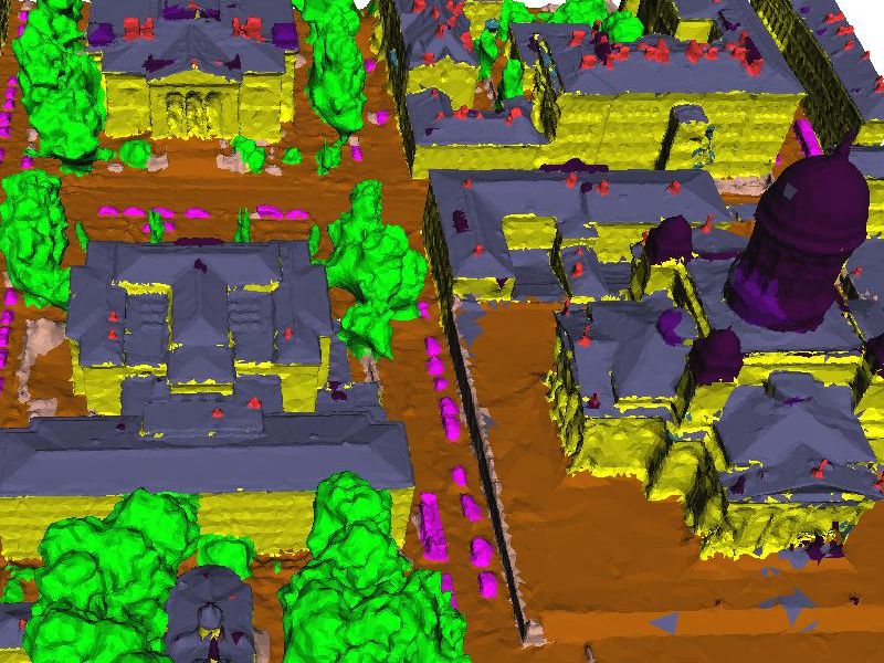
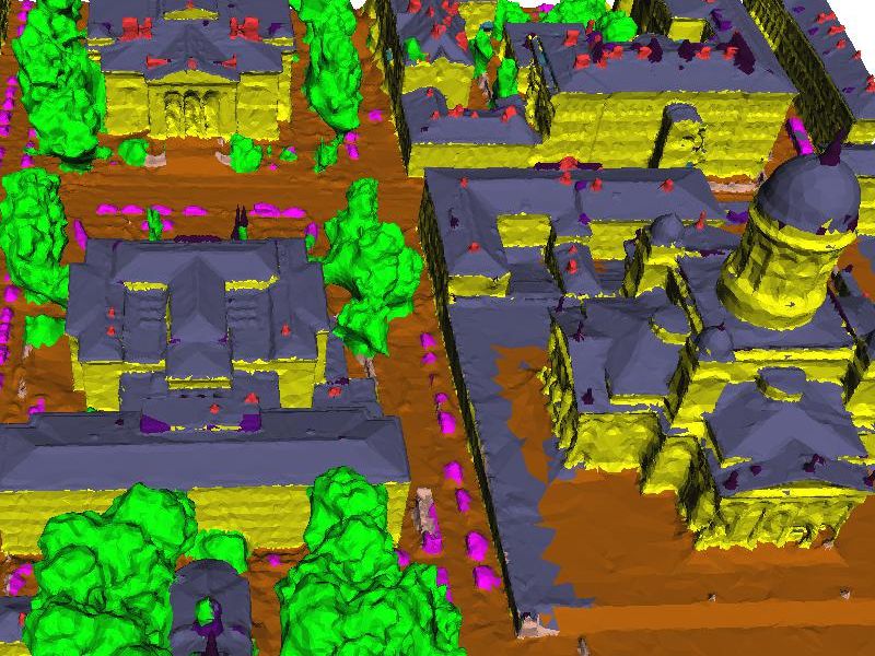
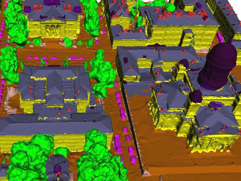
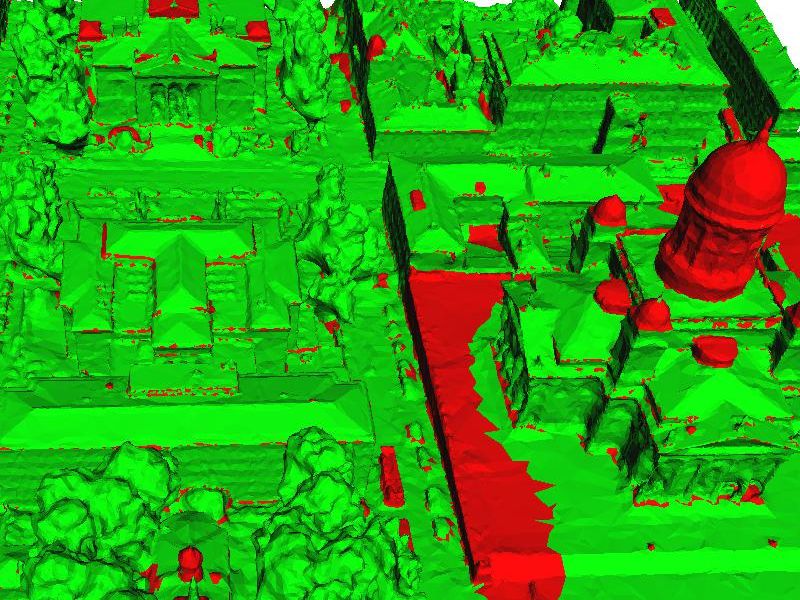
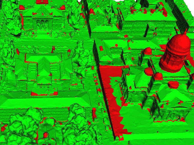
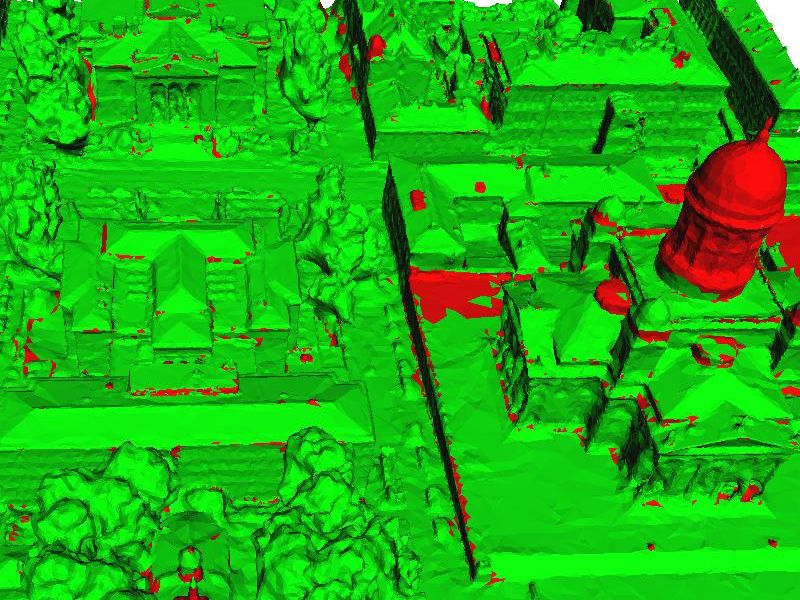
KPConvFc.	PointNextFc.	PointTransV3Fc.	PointVectorFc.

Figure 22: Qualitative analysis of semantic segmentation and error maps in the face labeling track for all methods except PointNet [12] in the second scenario. ^Fc. and ^Sp. denote face-centered and superpixel sampling, respectively.

Truth (top), Mesh (bottom)	PointNetSp.	PointNet++Sp.	SPGSp.	SparseUNetRd.
Randla-netSp.	KPConvSp.	PointNextPo.	PointTransV3Rd.	PointVectorSp.
Truth (top), Mesh (bottom)	PointNetSp.	PointNet++Sp.	SPGSp.	SparseUNetRd.
Randla-netSp.	KPConvSp.	PointNextPo.	PointTransV3Rd.	PointVectorSp.

Figure 23: Qualitative analysis of semantic segmentation and error maps in the pixel labeling track for all methods in the first scenario. ^Sp. denotes superpixel sampling, ^Rd. for random sampling, and ^Po. for Poisson-disk sampling [14]. The zoomed-in view direction is indicated in the input mesh image.

Truth (top), Mesh (bottom)	PointNetSp.	PointNet++Sp.	SPGSp.	SparseUNetRd.
Randla-netSp.	KPConvSp.	PointNextPo.	PointTransV3Rd.	PointVectorSp.
Truth (top), Mesh (bottom)	PointNetSp.	PointNet++Sp.	SPGSp.	SparseUNetRd.
Randla-netSp.	KPConvSp.	PointNextPo.	PointTransV3Rd.	PointVectorSp.

Figure 24: Qualitative analysis of semantic segmentation and error maps in the pixel labeling track for all methods in the second scenario. ^Sp. denotes superpixel sampling, ^Rd. for random sampling, and ^Po. for Poisson-disk sampling [14]. The zoomed-in view direction is indicated in the input mesh image.

8 Comparison of related datasets

Compare with SUM.

Our proposed SUM Parts dataset extends beyond SUM’s object-level labels [19], offering three key benefits: (1) finer geometric analysis, such as evaluating heat loss at the window-level rather than at the building-scale; (2) support for part-aware tasks, e.g., drone navigation for precise delivery by localizing windows, doors, and rooftop solar panel planning; (3) seamless integration with urban digital twins and BIM workflows.

Compare with KITTI-360.

KITTI-360 [35] focuses on street-view LiDAR-image fusion for autonomous driving, providing 37 Cityscapes-aligned classes, including road-accessible static and dynamic objects ($\geq$0.1m resolution) labeled via manual selection and trajectory-based matching. In contrast, SUM Parts addresses broader urban planning and sustainability challenges using oblique photogrammetry meshes. Key differences include: (1) Labeling granularity: SUM Parts offers both object- and part-level annotations (21 CityGML-aligned classes) for fine-grained urban infrastructure details. (2) Annotation tools: Our mesh-texture semi-automatic selection tools (click, stroke, lasso) with 2D/3D template matching ensure efficient annotation. (3) Coverage: SUM Parts provides full-city coverage, annotating all static objects ($\geq$0.5m resolution), including vehicle-inaccessible areas. Hence, SUM Parts complements KITTI-360 for broader urban applications.

References

- Achanta et al. [2012] Radhakrishna Achanta, Appu Shaji, Kevin Smith, Aurelien Lucchi, Pascal Fua, and Sabine Süsstrunk. SLIC superpixels compared to state-of-the-art superpixel methods. IEEE Transactions on Pattern Analysis and Machine Intelligence, 34(11):2274–2282, 2012.
- Adams and Bischof [1994] R. Adams and L. Bischof. Seeded region growing. IEEE Transactions on Pattern Analysis and Machine Intelligence, 16(6):641–647, 1994.
- AHN [2019] AHN. Actueel Hoogtebestand Nederland (AHN). https://www.ahn.nl/, 2019. Accessed: 2021-04-16.
- Airaksinen et al. [2019] E. Airaksinen, M. Bergström, H. Heinonen, K. Kaisla, K. Lahti, and J. Suomisto. The Kalasatama digital twins project—The final report of the KIRA-digi pilot project. Technical report, City of Helsinki, 2019.
- Armeni et al. [2017] I. Armeni, A. Sax, A. R. Zamir, and S. Savarese. Joint 2D-3D-semantic data for indoor scene understanding. ArXiv e-prints, 2017.
- Boykov and Jolly [2001] Y.Y. Boykov and M.-P. Jolly. Interactive graph cuts for optimal boundary & region segmentation of objects in N-D images. In Proceedings Eighth IEEE International Conference on Computer Vision. ICCV 2001, pages 105–112 vol.1, 2001.
- Boykov et al. [2001] Y. Boykov, O. Veksler, and R. Zabih. Fast approximate energy minimization via graph cuts. IEEE Transactions on Pattern Analysis and Machine Intelligence, 23(11):1222–1239, 2001.
- Briechle and Hanebeck [2001] Kai Briechle and Uwe D Hanebeck. Template matching using fast normalized cross correlation. In Optical pattern recognition XII, pages 95–102. SPIE, 2001.
- Brostow et al. [2009] Gabriel J. Brostow, Julien Fauqueur, and Roberto Cipolla. Semantic object classes in video: A high-definition ground truth database. Pattern Recognition Letters, 30(2):88–97, 2009. Video-based Object and Event Analysis.
- Can et al. [2021] Gülcan Can, Dario Mantegazza, Gabriele Abbate, Sébastien Chappuis, and Alessandro Giusti. Semantic segmentation on swiss3Dcities: A benchmark study on aerial photogrammetric 3D pointcloud dataset. Pattern Recognition Letters, 150:108–114, 2021.
- Chang et al. [2017] Angel Chang, Angela Dai, Thomas Funkhouser, Maciej Halber, Matthias Niessner, Manolis Savva, Shuran Song, Andy Zeng, and Yinda Zhang. Matterport3D: Learning from RGB-D data in indoor environments. International Conference on 3D Vision (3DV), 2017.
- Charles et al. [2017] R. Qi Charles, Hao Su, Mo Kaichun, and Leonidas J. Guibas. PointNet: Deep learning on point sets for 3D classification and segmentation. In 2017 IEEE Conference on Computer Vision and Pattern Recognition (CVPR), pages 77–85, 2017.
- Cheng et al. [2021] Bowen Cheng, Ross Girshick, Piotr Dollár, Alexander C. Berg, and Alexander Kirillov. Boundary IoU: Improving object-centric image segmentation evaluation. In 2021 IEEE/CVF Conference on Computer Vision and Pattern Recognition (CVPR), pages 15329–15337, 2021.
- Cook [1986] Robert L. Cook. Stochastic sampling in computer graphics. ACM Trans. Graph., 5(1):51–72, 1986.
- Cordts et al. [2016] M. Cordts, M. Omran, S. Ramos, T. Rehfeld, M. Enzweiler, R. Benenson, U. Franke, S. Roth, and B. Schiele. The cityscapes dataset for semantic urban scene understanding. In 2016 IEEE Conference on Computer Vision and Pattern Recognition (CVPR), pages 3213–3223, Los Alamitos, CA, USA, 2016. IEEE Computer Society.
- Dai et al. [2017] Angela Dai, Angel X. Chang, Manolis Savva, Maciej Halber, Thomas Funkhouser, and Matthias Nießner. ScanNet: Richly-annotated 3D reconstructions of indoor scenes. In 2017 IEEE Conference on Computer Vision and Pattern Recognition (CVPR), pages 2432–2443, 2017.
- Deng et al. [2023] Xin Deng, WenYu Zhang, Qing Ding, and XinMing Zhang. Pointvector: A vector representation in point cloud analysis. In 2023 IEEE/CVF Conference on Computer Vision and Pattern Recognition (CVPR), pages 9455–9465, 2023.
- Fei et al. [2022] Ben Fei, Weidong Yang, Wen-Ming Chen, Zhijun Li, Yikang Li, Tao Ma, Xing Hu, and Lipeng Ma. Comprehensive review of deep learning-based 3D point cloud completion processing and analysis. IEEE Transactions on Intelligent Transportation Systems, 23(12):22862–22883, 2022.
- Gao et al. [2021] Weixiao Gao, Liangliang Nan, Bas Boom, and Hugo Ledoux. SUM: A benchmark dataset of Semantic Urban Meshes. ISPRS Journal of Photogrammetry and Remote Sensing, 179:108–120, 2021.
- Gao et al. [2023] Weixiao Gao, Liangliang Nan, Bas Boom, and Hugo Ledoux. PSSNet: Planarity-sensible semantic segmentation of large-scale urban meshes. ISPRS Journal of Photogrammetry and Remote Sensing, 196:32–44, 2023.
- Grady [2006] L. Grady. Random walks for image segmentation. IEEE Transactions on Pattern Analysis and Machine Intelligence, 28(11):1768–1783, 2006.
- Graham et al. [2018] Benjamin Graham, Martin Engelcke, and Laurens van der Maaten. 3D semantic segmentation with submanifold sparse convolutional networks. In 2018 IEEE/CVF Conference on Computer Vision and Pattern Recognition, pages 9224–9232, 2018.
- Gröger and Plümer [2012] Gerhard Gröger and Lutz Plümer. CityGML – interoperable semantic 3D city models. ISPRS Journal of Photogrammetry and Remote Sensing, 71:12–33, 2012.
- Hackel et al. [2017] T. Hackel, N. Savinov, L. Ladicky, J. D. Wegner, K. Schindler, and M. Pollefeys. Semantic3d.net: A new large-scale point cloud classification benchmark. ISPRS Annals of the Photogrammetry, Remote Sensing and Spatial Information Sciences, IV-1/W1:91–98, 2017.
- Hu et al. [2020] Qingyong Hu, Bo Yang, Linhai Xie, Stefano Rosa, Yulan Guo, Zhihua Wang, Niki Trigoni, and Andrew Markham. RandLA-Net: Efficient semantic segmentation of large-scale point clouds. In 2020 IEEE/CVF Conference on Computer Vision and Pattern Recognition (CVPR), pages 11105–11114, 2020.
- Ibrahim et al. [2021] Muhammad Ibrahim, Naveed Akhtar, Michael Wise, and Ajmal Mian. Annotation tool and urban dataset for 3D point cloud semantic segmentation. IEEE Access, 9:35984–35996, 2021.
- Kirillov et al. [2023] Alexander Kirillov, Eric Mintun, Nikhila Ravi, Hanzi Mao, Chloe Rolland, Laura Gustafson, Tete Xiao, Spencer Whitehead, Alexander C. Berg, Wan-Yen Lo, Piotr Dollár, and Ross Girshick. Segment anything. In 2023 IEEE/CVF International Conference on Computer Vision (ICCV), pages 3992–4003, 2023.
- Kölle et al. [2021] Michael Kölle, Dominik Laupheimer, Stefan Schmohl, Norbert Haala, Franz Rottensteiner, Jan Dirk Wegner, and Hugo Ledoux. The Hessigheim 3D (H3D) benchmark on semantic segmentation of high-resolution 3D point clouds and textured meshes from UAV LiDAR and Multi-View-Stereo. ISPRS Open Journal of Photogrammetry and Remote Sensing, 1:100001, 2021.
- Kontogianni et al. [2023] Theodora Kontogianni, Ekin Celikkan, Siyu Tang, and Konrad Schindler. Interactive object segmentation in 3D point clouds. In 2023 IEEE International Conference on Robotics and Automation (ICRA), pages 2891–2897, 2023.
- Landrieu and Simonovsky [2018] Loic Landrieu and Martin Simonovsky. Large-scale point cloud semantic segmentation with superpoint graphs. In 2018 IEEE/CVF Conference on Computer Vision and Pattern Recognition, pages 4558–4567, 2018.
- Lang et al. [2024] Itai Lang, Fei Xu, Dale Decatur, Sudarshan Babu, and Rana Hanocka. iSeg: Interactive 3D segmentation via interactive attention. In SIGGRAPH Asia 2024 Conference Papers, New York, NY, USA, 2024. Association for Computing Machinery.
- Li et al. [2023] Feng Li, Hao Zhang, Huaizhe Xu, Shilong Liu, Lei Zhang, Lionel M. Ni, and Heung-Yeung Shum. Mask DINO: Towards a unified transformer-based framework for object detection and segmentation. In 2023 IEEE/CVF Conference on Computer Vision and Pattern Recognition (CVPR), pages 3041–3050, Los Alamitos, CA, USA, 2023. IEEE Computer Society.
- Li et al. [2025] Feng Li, Hao Zhang, Peize Sun, Xueyan Zou, Shilong Liu, Chunyuan Li, Jianwei Yang, Lei Zhang, and Jianfeng Gao. Segment and recognize anything at any granularity. In Computer Vision – ECCV 2024, pages 467–484, Cham, 2025. Springer Nature Switzerland.
- Li et al. [2020] Xinke Li, Chongshou Li, Zekun Tong, Andrew Lim, Junsong Yuan, Yuwei Wu, Jing Tang, and Raymond Huang. Campus3D: A photogrammetry point cloud benchmark for hierarchical understanding of outdoor scene. In Proceedings of the 28th ACM International Conference on Multimedia, page 238–246, New York, NY, USA, 2020. Association for Computing Machinery.
- Liao et al. [2023] Yiyi Liao, Jun Xie, and Andreas Geiger. KITTI-360: A novel dataset and benchmarks for urban scene understanding in 2D and 3D. IEEE Transactions on Pattern Analysis and Machine Intelligence, 45(3):3292–3310, 2023.
- Liu and Boehm [2014] K. Liu and J. Boehm. A new framework for interactive segmentation of point clouds. The International Archives of the Photogrammetry, Remote Sensing and Spatial Information Sciences, XL-5:357–362, 2014.
- Liu et al. [2023] Q. Liu, Z. Xu, G. Bertasius, and M. Niethammer. Simpleclick: Interactive image segmentation with simple vision transformers. In 2023 IEEE/CVF International Conference on Computer Vision (ICCV), pages 22233–22243, Los Alamitos, CA, USA, 2023. IEEE Computer Society.
- Luo et al. [2001] M Ronnier Luo, Guihua Cui, and Bryan Rigg. The development of the CIE 2000 colour-difference formula: CIEDE2000. Color Research & Application: Endorsed by Inter-Society Color Council, The Colour Group (Great Britain), Canadian Society for Color, Color Science Association of Japan, Dutch Society for the Study of Color, The Swedish Colour Centre Foundation, Colour Society of Australia, Centre Français de la Couleur, 26(5):340–350, 2001.
- Maninis et al. [2018] K. Maninis, S. Caelles, J. Pont-Tuset, and L. Van Gool. Deep extreme cut: From extreme points to object segmentation. In 2018 IEEE/CVF Conference on Computer Vision and Pattern Recognition (CVPR), pages 616–625, Los Alamitos, CA, USA, 2018. IEEE Computer Society.
- Martinović et al. [2015] Anđelo Martinović, Jan Knopp, Hayko Riemenschneider, and Luc Van Gool. 3D all the way: Semantic segmentation of urban scenes from start to end in 3D. In 2015 IEEE Conference on Computer Vision and Pattern Recognition (CVPR), pages 4456–4465, 2015.
- McKinnon and Hoff [2017] Tom McKinnon and Paul Hoff. Comparing RGB-based vegetation indices with NDVI for drone based agricultural sensing. Agribotix. Com, 21(17):1–8, 2017.
- Miksik et al. [2015] Ondrej Miksik, Vibhav Vineet, Morten Lidegaard, Ram Prasaath, Matthias Nießner, Stuart Golodetz, Stephen L. Hicks, Patrick Pérez, Shahram Izadi, and Philip H.S. Torr. The semantic paintbrush: Interactive 3D mapping and recognition in large outdoor spaces. In Proceedings of the 33rd Annual ACM Conference on Human Factors in Computing Systems, page 3317–3326, New York, NY, USA, 2015. Association for Computing Machinery.
- Mortensen and Barrett [1998] Eric N. Mortensen and William A. Barrett. Interactive segmentation with intelligent scissors. Graphical Models and Image Processing, 60(5):349–384, 1998.
- Ning et al. [2010] Jifeng Ning, Lei Zhang, David Zhang, and Chengke Wu. Interactive image segmentation by maximal similarity based region merging. Pattern Recognition, 43(2):445–456, 2010. Interactive Imaging and Vision.
- OGC [2021] OGC. OGC City Geography Markup Language (CityGML) Part 1: Conceptual Model Standard. Open Geospatial Consortium inc., 2021. Document 20-010, version 3.0.0, available at https://docs.ogc.org/is/20-010/20-010.html.
- Peters [2018] Ravi Peters. Geographical point cloud modelling with the 3D medial axis transform. PhD thesis, Technische Universiteit Delft, 2018.
- Qi et al. [2017] Charles R. Qi, Li Yi, Hao Su, and Leonidas J. Guibas. PointNet++: Deep hierarchical feature learning on point sets in a metric space. In Proceedings of the 31st International Conference on Neural Information Processing Systems, page 5105–5114, Red Hook, NY, USA, 2017. Curran Associates Inc.
- Qian et al. [2022] Guocheng Qian, Yuchen Li, Houwen Peng, Jinjie Mai, Hasan Hammoud, Mohamed Elhoseiny, and Bernard Ghanem. PointNext: Revisiting PointNet++ with improved training and scaling strategies. In Advances in Neural Information Processing Systems, pages 23192–23204. Curran Associates, Inc., 2022.
- Romanoni and Matteucci [2018] A. Romanoni and M. Matteucci. A data-driven prior on facet orientation for semantic mesh labeling. In 2018 International Conference on 3D Vision (3DV), pages 662–671, Los Alamitos, CA, USA, 2018. IEEE Computer Society.
- Rother et al. [2004] Carsten Rother, Vladimir Kolmogorov, and Andrew Blake. GrabCut: interactive foreground extraction using iterated graph cuts. ACM Trans. Graph., 23(3):309–314, 2004.
- Rouhani et al. [2017a] Mohammad Rouhani, Florent Lafarge, and Pierre Alliez. Semantic segmentation of 3D textured meshes for urban scene analysis. ISPRS Journal of Photogrammetry and Remote Sensing, 123:124–139, 2017a.
- Rouhani et al. [2017b] Mohammad Rouhani, Florent Lafarge, and Pierre Alliez. Semantic segmentation of 3D textured meshes for urban scene analysis. ISPRS Journal of Photogrammetry and Remote Sensing, 123:124–139, 2017b.
- Roynard et al. [2018] Xavier Roynard, Jean-Emmanuel Deschaud, and François Goulette. Paris-Lille-3D: A large and high-quality ground-truth urban point cloud dataset for automatic segmentation and classification. The International Journal of Robotics Research, 37(6):545–557, 2018.
- Schmitz et al. [2022] Patric Schmitz, Sebastian Suder, Kersten Schuster, and Leif Kobbelt. Interactive segmentation of textured point clouds. In Vision, Modeling, and Visualization. The Eurographics Association, 2022.
- Selvaraju et al. [2021] Pratheba Selvaraju, Mohamed Nabail, Marios Loizou, Maria Maslioukova, Melinos Averkiou, Andreas Andreou, Siddhartha Chaudhuri, and Evangelos Kalogerakis. BuildingNet: Learning to label 3D buildings. In 2021 IEEE/CVF International Conference on Computer Vision (ICCV), pages 10377–10387, 2021.
- Sherbrooke et al. [1996] E.C. Sherbrooke, N.M. Patrikalakis, and E. Brisson. An algorithm for the medial axis transform of 3d polyhedral solids. IEEE Transactions on Visualization and Computer Graphics, 2(1):44–61, 1996.
- SYSTEMS [2016] BENTLEY SYSTEMS. Reality and spatial modeling software. https://www.bentley.com/software/reality-and-spatial-modeling/, 2016. Accessed: 2025-03-14.
- Thomas et al. [2019] Hugues Thomas, Charles R. Qi, Jean-Emmanuel Deschaud, Beatriz Marcotegui, François Goulette, and Leonidas Guibas. KPConv: Flexible and deformable convolution for point clouds. In 2019 IEEE/CVF International Conference on Computer Vision (ICCV), pages 6410–6419, 2019.
- Weinmann et al. [2013] Martin Weinmann, Boris Jutzi, and Clément Mallet. Feature relevance assessment for the semantic interpretation of 3D point cloud data. ISPRS Workshop Laser Scanning 2013. ISPRS Annals of the Photogrammetry, Remote Sensing and Spatial Information Sciences, Vol. II-5/W2, pages 313–318, 2013.
- Wu et al. [2024] Xiaoyang Wu, Li Jiang, Peng-Shuai Wang, Zhijian Liu, Xihui Liu, Yu Qiao, Wanli Ouyang, Tong He, and Hengshuang Zhao. Point Transformer V3: Simpler, Faster, Stronger . In 2024 IEEE/CVF Conference on Computer Vision and Pattern Recognition (CVPR), pages 4840–4851, Los Alamitos, CA, USA, 2024. IEEE Computer Society.
- Yue et al. [2024] Yuanwen Yue, Sabarinath Mahadevan, Jonas Schult, Francis Engelmann, Bastian Leibe, Konrad Schindler, and Theodora Kontogianni. AGILE3D: Attention Guided Interactive Multi-object 3D Segmentation. In International Conference on Learning Representations (ICLR), 2024.
- Zolanvari et al. [2019] SM Zolanvari, Susana Ruano, Aakanksha Rana, Alan Cummins, Rogerio Eduardo da Silva, Morteza Rahbar, and Aljosa Smolic. DublinCity: Annotated LiDAR point cloud and its applications. In BMVC 30th British Machine Vision Conference, 2019.