A Sigma Point-based Low Complexity Algorithm for Multipath-based SLAM in MIMO Systems

Abstract

mpslam is a promising approach in wireless networks to jointly obtain position information of transmitters/receivers and information of the propagation environment. mpslam models specular reflections at flat surfaces as virtual anchors, which are mirror images of base stations. Particle-based methods offer high flexibility and can approximate posterior probability density functions with complex shapes. However, they often require a large number of particles to counteract degeneracy in high-dimensional parameter spaces, leading to high runtimes. Conversely using too few particles leads to reduced estimation accuracy. In this paper, we propose a low-complexity algorithm for multipath-based simultaneous localization and mapping (MP-SLAM) in MIMO systems that employs sigma point (SP) approximations via the sum-product algorithm (SPA). Specifically, we use Gaussian approximations through SP-transformations, drastically reducing computational overhead without sacrificing accuracy. Nonlinearities are handled by SP updates, and moment matching approximates the Gaussian mixtures arising from probabilistic data association (PDA). Numerical results show that our method achieves considerably shorter runtimes than particle-based schemes, with comparable or even superior performance.

I Introduction

Emerging sensing and signal processing techniques that exploit multipath propagation promise advanced capabilities in autonomous navigation, asset localization, and situational awareness for future communication networks. mpslam effectively tracks mobile transmitters or receivers while mapping the environment in wireless systems by modelling specular reflections of RF signals as VAs, which are mirror images of BSs or static transceivers called physical anchors (see Fig. 1) [1, 2, 3, 4, 5].

MP-SLAM falls under the umbrella of feature-based SLAM approaches, which focus on detecting and mapping distinct environmental features [6, 7]. MP-SLAM facilitates a factor graph (FG)-based representation of the joint posterior density and uses the SPA to solve the MP-SLAM problem in a Bayesian manner. It allows to solve the PDA problem inherent to MP-SLAM with high scalability and was shown to offer a superior trade-off between robustness and runtime [3, 4, 8, 9]. MP-SLAM has been successfully applied to a variety of different scenarios, including cooperative localization [10], the use of adaptive map feature models [11], and environments that involve reflections from rough surfaces [12]. Most MP-SLAM methods use particle-based implementations [13] to represent the joint posterior distribution [4, 8, 9, 3]. Particle-based methods offer high flexibility and can provide an asymptotically optimal approximation of posterior PDFs with complex shapes. This property is particularly useful for highly nonlinear and reduced information scenarios, such as time-of-arrival (TOA)-only MP-SLAM, where the inherent physics of the problem can induce strongly non-Gaussian PDFs [4]. While the factor graph-based approach to MP-SLAM allows for significant reduction of the problem complexity, it typically still requires a high number of particles to counteract degeneracy in high-dimensional parameter spaces, leading to high runtimes; conversely using too few particles leads to reduced estimation accuracy. In multiple input multiple output (MIMO) systems, array measurements enable jointly estimating TOA, angle-of-arrival (AOA) and angle-of-arrival (AOD). The additional information contained in AOA and AOD estimates can yield unambiguous measurement transformations, allowing the resulting joint posterior PDF to be approximated accurately by Gaussian densities. A popular method for approximating PDFs that arise from nonlinear transformations is the unscented or SP transform [14, 15, 16], which has been shown to offer superior approximation performance compared to first-order Taylor linearization employed by Kalman Filter (KF)-type methods.

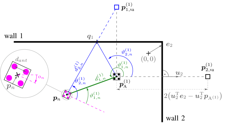
Figure 1: Exemplary indoor environment including the mobile agent at position $\bm{p}_{n}$, a PA at position $\bm{p}^{(1)}_{\text{A}}$ and two corresponding VAs at position $\bm{p}_{1,\text{va}}^{(1)}$ and $\bm{p}_{2,\text{va}}^{(2)}$. The visualization includes the array geometry used by the agent and PAs, along with the geometric relationships between the objects.

In this paper, we propose an SP-based implementation of the SPA algorithm for MP-SLAM. By approximating all PDFs using SPs, we efficiently evaluate the integrals required by the algorithm. We describe in detail the steps involved in this approximation, emphasizing the handling of nonlinearities in both the state transition and the measurement models, and discuss the use of moment matching to approximate Gaussian mixtures arising from data association. The main contributions of this paper are as follows.

• We propose a novel SP-based implementation of the SPA algorithm for MP-SLAM.

• We leverage Gaussian approximations of all PDFs by means of SPs, enabling efficient evaluation of the integrals required by the algorithm and we provide a detailed derivation of these approximations.

• We validate our method demonstrating significantly lower runtimes compared to a particle-based implementation [4, 8, 17] and also improved accuracy in certain cases.

Notations and Definitions: column vectors and matrices are denoted by boldface lowercase and uppercase letters. Random variables are displayed in san serif, upright font, e.g., $\mathsfbr{x}$ and $\bm{\mathsfbr{x}}$ and their realizations in serif, italic font, e.g. $x$. $f({x})$ and $p({x})$ denote, respectively, the PDF or probability mass function (PMF) of a continuous or discrete random variable $\mathsfbr{x}$ (these are short notations for $f{x}({x})$ or $p{x}({x})$). $(\cdot)^{\mathrm{T}}$, denotes the matrix transpose. $\lVert\cdot\rVert$ is the Euclidean norm. $|\cdot|$ represents the cardinality of a set. $\operatorname{blkdiag}\{\bm{A},\bm{B}\}$ denotes a block-diagonal matrix with $\bm{A}$ and $\bm{B}$ on the diagonal and zero matrices in the off-diagonal blocks. $\bm{I}_{[\cdot]}$ is an identity matrix of dimension given in the subscript. Furthermore, ${1}_{\mathbb{A}}(\bm{x})$ denotes the indicator function that is ${1}_{\mathbb{A}}(\bm{x})=1$ if $\bm{x}\in\mathbb{A}$ and 0 otherwise, for $\mathbb{A}$ being an arbitrary set and $\mathbb{R}^{\text{+}}$ is the set of positive real numbers. The Gaussian PDF is $f_{\text{N}}(x;\mu,\sigma)=1/(\sqrt{2\pi}\sigma){e}^{(-(x-\mu)^{2}/(2\sigma^{2}))}$ with mean $\mu$, standard deviation $\sigma$ and the uniform PDF $f_{\mathrm{U}}(x;a,b)=1/(b-a){1}_{[a,b]}(x)$.

II System Setup and Geometrical Relations

At each time step $n$, we consider a mobile agent located at position $\bm{p}_{n}\triangleq[{p}_{\text{x}\hskip 0.5ptn}\;{p}_{\text{y}\hskip 0.5ptn}]^{\text{T}}$, equipped with $\sqrt{N_{\text{ant}}}$ times $\sqrt{N_{\text{ant}}}$ uniform planar array (UPA) with $N_{\text{ant}}$ antenna elements spaced distance $d_{\text{ant}}$ apart and oriented at angle $\kappa_{n}$. Similarly, $J$ BSs acting as PAs and placed at fixed positions $\bm{p}_{\text{A}}^{(j)}\triangleq[{p}_{\text{x\hskip 0.5ptA}}^{(j)}\;{p}_{\text{y\hskip 0.5ptA}}^{(j)}]^{\text{T}}$ are also equipped with an $N_{\text{ant}}^{(j)}$-element UPA, with spacing $d_{\text{ant}}^{(j)}$. A radio signal $\bm{r}_{n}^{(j)}$ transmitted by the mobile agent at carrier frequency $f_{\text{c}}$ and with signal-bandwidth $B$ arrives at the receiver via the line-of-sight (LOS) path as well as via multipath components originating from the reflection of surrounding objects.

II-1 Feature Model

Reflections caused by flat surfaces are modelled by VAs [9, 5, 12], mirroring the position of the physical anchors on the respective surfaces, located at $\bm{p}_{k,\mathrm{va}}^{(j)}=\bm{p}_{n}+2(\bm{u}_{k}^{\text{T}}\bm{e}_{k}-\bm{u}_{k}^{\text{T}}\bm{p}_{\text{A}}^{(j)})\bm{u}_{k}$ for first-order reflections, with the vector $\bm{e}_{k}$ pointing from the coordinate origin to the surface $k$ and the unit vector $\bm{u}_{k}$ normal to that same surface. For notational conciseness, PAs positions will be referred to as $\bm{p}_{\text{A}}^{(j)}\triangleq\bm{p}_{1,\mathrm{va}}^{(j)}$. Further, we denote the distance between the agent and any anchor as $d_{k,n}^{(j)}\triangleq d(\bm{p}_{n},\bm{p}_{k,\mathrm{va}}^{(j)})=||\bm{p}_{n}-\bm{p}_{k,\mathrm{va}}^{(j)}||$, the AOA as $\theta_{k,n}^{(j)}\triangleq\angle{(\bm{p}_{n},\bm{p}_{k,\mathrm{va}}^{(j)})}+\kappa_{n}=\operatorname{atan2}{({p}_{\text{y\hskip 0.5ptA}}^{(j)}-{p}_{\text{y}\hskip 0.5ptn},{p}_{\text{x\hskip 0.5ptA}}^{(j)}-{p}_{\text{x}\hskip 0.5ptn})}+\kappa_{n}$ and the AOD as $\vartheta_{k,n}^{(j)}=\angle{(\bm{p}_{n},\bm{p}_{\text{A}}^{(j)})}=\operatorname{atan2}{({p}_{\text{y}\hskip 0.5ptn}-{p}_{\text{y\hskip 0.5ptA}}^{(j)},{p}_{\text{x}\hskip 0.5ptn}-{p}_{\text{x\hskip 0.5ptA}}^{(j)})}$ for PAs and $\vartheta_{k,n}^{(j)}=\angle{(\bm{p}_{n},\bm{q}_{k,n}^{(j)})}=\operatorname{atan2}{({p}_{\text{y}\hskip 0.5ptn}-{p}_{\text{y}\hskip 0.5ptk,n}^{(j)},{p}_{\text{x}\hskip 0.5ptn}-{p}_{\text{x}\hskip 0.5ptk,n}^{(j)})}$ for VAs (see Fig. 1). The reflection point $\bm{q}_{k,n}^{(j)}\triangleq[{p}_{\text{x}\hskip 0.5ptk,n}^{(j)}\;{p}_{\text{y}\hskip 0.5ptk,n}^{(j)}]^{\text{T}}$, needed to relate the AOD to a VA is given by

$$\bm{q}_{k,n}^{(j)}=\bm{p}_{k,\mathrm{va}}^{(j)}+\frac{(\bm{p}_{\text{A}}^{(j)}-\bm{p}_{k,\mathrm{va}}^{(j)})^{\mathrm{T}}\bm{u}_{k}}{2(\bm{p}_{n}-\bm{p}_{k,\mathrm{va}}^{(j)})^{\mathrm{T}}\bm{u}_{k}}(\bm{p}_{n}-\bm{p}_{k,\mathrm{va}}^{(j)}).$$ (1)

II-2 Measurement Extraction

For each time $n$ and anchor $j$, a channel estimation and detection algorithm (CEDA) [18, 19, 20, 21] extracts an unknown number of measurements $m\in{\cal{M}}_{n}^{(j)}\triangleq\{1,\,\dots\,,M_{n}^{(j)}\}$ from a received RF signal vector $\bm{r}_{n}^{(j)}$. Each measurement $\bm{z}^{(j)}_{m,n}=[{z_{\mathrm{d}}^{(j)}}_{\hskip-0.85358pt\hskip-0.85358pt\hskip-0.85358pt\hskip-0.85358pt\hskip-0.85358pt\hskip-0.85358pt\hskip-0.85358ptm,n}\;{z_{\mathrm{\theta}}^{(j)}}_{\hskip-0.85358pt\hskip-0.85358pt\hskip-0.85358pt\hskip-0.85358pt\hskip-0.85358pt\hskip-0.85358pt\hskip-0.85358ptm,n}\;{z_{\mathrm{\vartheta}}^{(j)}}_{\hskip-0.85358pt\hskip-0.85358pt\hskip-0.85358pt\hskip-0.85358pt\hskip-0.85358pt\hskip-0.85358pt\hskip-0.85358ptm,n}\;{z_{\mathrm{u}}^{(j)}}_{\hskip-0.85358pt\hskip-0.85358pt\hskip-0.85358pt\hskip-0.85358pt\hskip-0.85358pt\hskip-0.85358pt\hskip-0.85358ptm,n}]^{\mathrm{T}}$ contains a distance ${z_{\mathrm{d}}^{(j)}}_{\hskip-0.85358pt\hskip-0.85358pt\hskip-0.85358pt\hskip-0.85358pt\hskip-0.85358pt\hskip-0.85358pt\hskip-0.85358ptm,n}=[0,d_{\text{max}}]$, AOA ${z_{\mathrm{\theta}}^{(j)}}_{\hskip-0.85358pt\hskip-0.85358pt\hskip-0.85358pt\hskip-0.85358pt\hskip-0.85358pt\hskip-0.85358pt\hskip-0.85358ptm,n}=[-\pi,\pi]$, AOD ${z_{\mathrm{\vartheta}}^{(j)}}_{\hskip-0.85358pt\hskip-0.85358pt\hskip-0.85358pt\hskip-0.85358pt\hskip-0.85358pt\hskip-0.85358pt\hskip-0.85358ptm,n}=[-\pi,\pi]$ and normalized amplitude ${z_{\mathrm{u}}^{(j)}}_{\hskip-0.85358pt\hskip-0.85358pt\hskip-0.85358pt\hskip-0.85358pt\hskip-0.85358pt\hskip-0.85358pt\hskip-0.85358ptm,n}=[\gamma,\infty)$ component, where $d_{\text{max}}$ is the maximum distance and $\gamma$ the detection threshold of the CEDA. In effect, channel estimation and detection is a compression of the information contained in $\bm{r}_{n}^{(j)}$ into the measurement vector ${\bm{z}^{(j)}_{n}}=[\bm{z}^{(j)\text{T}}_{1,n}\dots\bm{z}^{(j)\text{T}}_{{\cal{M}}_{n}^{(j)},n}]$. Note that in contrast to related work, such as [22, 23], in this work the amplitude ${z_{\mathrm{u}}^{(j)}}_{\hskip-0.85358pt\hskip-0.85358pt\hskip-0.85358pt\hskip-0.85358pt\hskip-0.85358pt\hskip-0.85358pt\hskip-0.85358ptm,n}$ is used exclusively to calculate the measurement variances of ${z_{\mathrm{d}}^{(j)}}_{\hskip-0.85358pt\hskip-0.85358pt\hskip-0.85358pt\hskip-0.85358pt\hskip-0.85358pt\hskip-0.85358pt\hskip-0.85358ptm,n}$, ${z_{\mathrm{\theta}}^{(j)}}_{\hskip-0.85358pt\hskip-0.85358pt\hskip-0.85358pt\hskip-0.85358pt\hskip-0.85358pt\hskip-0.85358pt\hskip-0.85358ptm,n}$, and ${z_{\mathrm{\vartheta}}^{(j)}}_{\hskip-0.85358pt\hskip-0.85358pt\hskip-0.85358pt\hskip-0.85358pt\hskip-0.85358pt\hskip-0.85358pt\hskip-0.85358ptm,n}$ according to [8].

III System Model

The state of the mobile agent is given as $\bm{\mathsfbr{x}}_{n}=[\bm{\mathsfbr{p}}_{n}^{\text{T}}\;\bm{\mathsfbr{v}}_{n}^{\text{T}}\;\bm{\skappa}_{n}]^{\text{T}}$, with its position $\bm{\mathsfbr{p}}_{n}=[\mathsfbr{p}_{\text{x},n}\;\mathsfbr{p}_{\text{y},n}]^{\text{T}}$, velocity $\bm{\mathsfbr{v}}_{n}=[\mathsfbr{v}_{\text{x},n}\;\mathsfbr{v}_{\text{y},n}]^{\text{T}}$, and orientation $\skappa_{n}$. In line with [4, 24], we account for an unknown number of VAs by introducing potential virtual anchors $k\in\{1,\dots,K_{n}^{(j)}\}\triangleq\mathcal{K}_{n}^{(j)}$. The PVA states are denoted as $\bm{\mathsfbr{y}}^{(j)}_{k,n}\triangleq[\bm{\spsi}^{(j)}_{k,n}{}^{\mathrm{T}}\;\mathsfbr{r}^{(j)}_{k,n}]^{\mathrm{T}}$, where $\bm{\spsi}^{(j)}_{k,n}$ represents the PVA position and $\mathsfbr{r}^{(j)}_{k,n}\in\{0,1\}$ is an existence variable modeling the existence/nonexistence of PVA $k$, i.e., $r^{(j)}_{k,n}=1$ if the PVA exists. Formally, its state is maintained even if PVA $k$ is nonexistent, i.e., if $r^{(j)}_{k,n}=0$. In that case, the position $\bm{\spsi}_{k,n}^{(j)}$ is irrelevant. Therefore, all PDFs defined for PVA states, $f(\bm{y}_{k,n}^{(j)})=f(\bm{\psi}_{k,n}^{(j)},r_{k,n}^{(j)})$, are of the form $f(\bm{\psi}_{k,n}^{(j)},r_{k,n}^{(j)}=0)=f_{k,n}^{(j)}\,f_{\mathrm{d}}(\bm{\psi}_{k,n}^{(j)})$, where $f_{\mathrm{d}}(\bm{\psi}_{k,n}^{(j)})$ is an arbitrary “dummy PDF,” and $f_{k,n}^{(j)}\in[0,1]$ is a constant representing the probability of non-existence [24, 4]. Note that for $k\in\{2,\dots,K_{n}^{(j)}\}$, the PVAs have unknown states $\bm{\mathsfbr{y}}^{(j)}_{k,n}$. In contrast, the PVA labeled $k=1$ represent the PA, whose position $\bm{\spsi}^{(j)}_{1,n}$ is assumed to be known. All PVAs states and agent states up to time $n$ are denoted as $\bm{\mathsfbr{y}}_{n}\!\triangleq[\bm{\mathsfbr{y}}_{n}^{(1)\text{T}}\hskip-0.85358pt\cdots\hskip 0.85358pt\bm{\mathsfbr{y}}_{n}^{(J)\text{T}}]^{\mathrm{T}}\hskip-0.85358pt$ and $\bm{\mathsfbr{y}}_{0:n}\!\triangleq[\bm{\mathsfbr{y}}_{0}^{\text{T}}\hskip-0.85358pt\cdots\hskip 0.85358pt\bm{\mathsfbr{y}}_{n}^{\text{T}}]^{\mathrm{T}}\hskip-0.85358pt$ and $\bm{\mathsfbr{x}}_{0:n}\!\triangleq[\bm{\mathsfbr{x}}_{0}^{\text{T}}\hskip-0.85358pt\cdots\hskip 0.85358pt\bm{\mathsfbr{x}}_{n}^{\text{T}}]^{\mathrm{T}}\hskip-0.85358pt$, respectively.

III-A State Evolution

The movement of the agent follows a linear model $\bm{\mathsfbr{x}}_{n}=\bm{A}\bm{\mathsfbr{x}}_{n-1}+\bm{\mathsfbr{w}}_{n}$, where $\bm{\mathsfbr{w}}_{n}$ is zero mean, Gaussian and i.i.d. across $n$, with covariance matrix $\bm{C}_{\text{x}}$, where we denote the associated state-transition distribution as $f(\bm{x}_{n}|\bm{x}_{n-1})$. We distinguish between two types of PVAs, based on their origin:

1. Legacy PVAs $\underline{\bm{\mathsfbr{y}}}_{k,n}^{(j)}$ ($k\hskip-0.85358pt\in\hskip-0.85358pt\mathcal{K}_{n-1}^{(j)}$) corresponding to PVAs that existed at the previous time $\underline{\bm{\mathsfbr{y}}}_{k,n-1}^{(j)}$.

2. New PVAs $\overline{\bm{\mathsfbr{y}}}_{m,n}^{(j)}$ ($m\hskip-0.85358pt\in\hskip-0.85358pt\mathcal{M}_{n}^{(j)}$) appearing at the current time $n$ for the first time[24, 4]. For each measurement $\bm{z}^{(j)}_{n}$ at time $n$ a new PVA is introduced.

Legacy PVAs evolve according to the joint state-transition PDF

$$f(\bm{x}_{n},\underline{\bm{y}}_{n}|\bm{x}_{n-1},\bm{y}_{n-1})$$

$$\hskip 42.67912pt=f(\bm{x}_{n}|\bm{x}_{n-1})\hskip-0.85358pt\hskip-0.85358pt\prod_{j=1}^{J}\prod_{k=1}^{K_{n-1}^{(j)}}\hskip-0.85358pt\hskip-0.85358pt\hskip-0.85358pt\hskip-0.85358ptf(\underline{\bm{y}}_{k,n}^{(j)}|\bm{y}_{k,n-1}^{(j)})$$ (2)

where $f(\underline{\bm{y}}_{k,n}^{(j)}|\bm{y}_{k,n-1}^{(j)})\hskip-0.85358pt\hskip-0.85358pt=\hskip-0.85358pt\hskip-0.85358ptf(\underline{\bm{\psi}}_{k,n}^{(j)},\underline{r}_{k,n}^{(j)}|\bm{\psi}_{k,n-1}^{(j)},r_{k,n-1}^{(j)})$ is the augmented state-transition PDF assuming that the augmented agent state as well as the PVA states evolve independently across $k$, $n$ and $j$ [24]. At time $n$, a PVA that existed at time $n-1$ either dies or survives with probability $p_{\mathrm{s}}$. In the case it does survive, its state is distributed according to the state-transition PDF $f(\underline{\bm{\psi}}_{k,n}^{(j)}|\bm{\psi}_{k,n-1}^{(j)})$, leading to

$$\hskip-0.85358pt\hskip-0.85358pt\hskip-0.85358pt\hskip-0.85358pt\hskip-0.85358pt\hskip-0.85358pt\hskip-0.85358ptf(\underline{\bm{\psi}}_{k,n}^{(j)},\underline{r}_{k,n}^{(j)}|\bm{\psi}_{k,n\text{-}1}^{(j)},1)\hskip-0.85358pt=\hskip-0.85358pt\hskip-0.85358pt\begin{cases}(1-p_{\mathrm{s}})f_{\mathrm{d}}(\underline{\bm{\psi}}_{k,n}^{(j)}),\hskip-0.85358pt\hskip-0.85358pt\hskip-0.85358pt\hskip-0.85358pt\hskip-0.85358pt&\underline{r}_{k,n}^{(j)}=0\\ p_{\mathrm{s}}f(\underline{\bm{\psi}}_{k,n}^{(j)}|\bm{\psi}_{k,n\text{-}1}^{(j)}),\hskip-0.85358pt\hskip-0.85358pt\hskip-0.85358pt\hskip-0.85358pt\hskip-0.85358pt&\underline{r}_{k,n}^{(j)}=1\end{cases}.\hskip-0.85358pt\hskip-0.85358pt\hskip-0.85358pt\hskip-0.85358pt\hskip-0.85358pt$$ (3)

If a PVA did not exist at time $n\hskip-0.85358pt\hskip-0.85358pt-\hskip-0.85358pt\hskip-0.85358pt1$, i.e., $r_{k,n-1}^{(j)}\hskip-0.85358pt\hskip-0.85358pt=\hskip-0.85358pt\hskip-0.85358pt0$, it cannot exist at time $n$ as a legacy PVA, meaning

$$f(\underline{\bm{\psi}}_{k,n}^{(j)},\underline{r}_{k,n}^{(j)}|\bm{\psi}_{k,n-1}^{(j)},0)=\begin{cases}f_{\mathrm{d}}(\underline{\bm{\psi}}_{k,n}^{(j)}),&\underline{r}_{k,n}^{(j)}=0\\ 0,&\underline{r}_{k,n}^{(j)}=1\end{cases}\,.$$ (4)

New PVAs are modeled by a Poisson point process with mean number of new PVA ${\mu}_{\mathrm{n}}$ and PDF $f_{\mathrm{n}}(\overline{\bm{\psi}}_{m,n}^{(j)})$, where ${\mu}_{\mathrm{n}}$ is assumed to be a known constant. Here, $\overline{r}_{m,n}^{(j)}=1$ indicates that the measurement $\bm{\mathsfbr{z}}_{m,n}^{(j)}$ was generated by a newly detected PVA. New PVAs become legacy PVAs at time $n+1$. Accordingly, the number of legacy PVAs is updated as $K_{n}^{(j)}=K_{n-1}^{(j)}+M_{n}^{(j)}$. To prevent the indefinite growth in the number of PVAs, PVA states with low existence probability (but not PAs) are removed, as described in Sec.  IV-A.

III-B Measurement Model

Prior to being observed, measurements ${\bm{\mathsfbr{z}}^{(j)}_{n}}$, and consequently their number $\mathsfbr{M}^{(j)}_{n}$, are considered random and are represented by the vector ${\bm{\mathsfbr{z}}^{(j)}_{n}}=[\bm{\mathsfbr{z}}^{(j)\text{T}}_{1,n}\dots\bm{\mathsfbr{z}}^{(j)\text{T}}_{\mathsfbr{M}_{n}^{(j)},n}]$. Both quantities are stacked into matrices containing all current measurements $\bm{\mathsfbr{z}}_{n}=[\bm{\mathsfbr{z}}^{(1)\,\text{T}}_{n}...\,\bm{\mathsfbr{z}}^{(J)\,\text{T}}_{n}]^{\text{T}}$ and their numbers $\bm{\mathsfbr{M}}_{n}=[\mathsfbr{M}^{(1)}_{n}\dots\mathsfbr{M}^{(J)}_{n}]$. We assume the likelihood function (LHF) of a measurement $f(\bm{z}_{m,n}^{(j)}|\bm{x}_{n},\bm{\psi}_{k,n}^{(j)})$ to be conditionally independent across its components ${z_{\mathrm{d}}^{(j)}}_{\hskip-0.85358pt\hskip-0.85358pt\hskip-0.85358pt\hskip-0.85358pt\hskip-0.85358pt\hskip-0.85358pt\hskip-0.85358ptm,n}$, ${z_{\mathrm{\theta}}^{(j)}}_{\hskip-0.85358pt\hskip-0.85358pt\hskip-0.85358pt\hskip-0.85358pt\hskip-0.85358pt\hskip-0.85358pt\hskip-0.85358ptm,n}$ and ${z_{\mathrm{\vartheta}}^{(j)}}_{\hskip-0.85358pt\hskip-0.85358pt\hskip-0.85358pt\hskip-0.85358pt\hskip-0.85358pt\hskip-0.85358pt\hskip-0.85358ptm,n}$, i.e.,

$$\hskip-0.85358ptf(\bm{z}_{m,n}^{(j)}|\bm{x}_{n},\bm{\psi}_{k,n}^{(j)})\hskip-0.85358pt =\hskip-0.85358ptf({z_{\mathrm{d}}^{(j)}}_{\hskip-0.85358pt\hskip-0.85358pt\hskip-0.85358pt\hskip-0.85358pt\hskip-0.85358pt\hskip-0.85358pt\hskip-0.85358ptm,n}|\bm{p}_{n},\bm{p}_{k,\mathrm{va}}^{(j)})\hskip 0.85358ptf({z_{\mathrm{\vartheta}}^{(j)}}_{\hskip-0.85358pt\hskip-0.85358pt\hskip-0.85358pt\hskip-0.85358pt\hskip-0.85358pt\hskip-0.85358pt\hskip-0.85358ptm,n}|\bm{p}_{n},\bm{p}_{k,\mathrm{va}}^{(j)})$$

$$\hskip 14.22636pt\times f({z_{\mathrm{\theta}}^{(j)}}_{\hskip-0.85358pt\hskip-0.85358pt\hskip-0.85358pt\hskip-0.85358pt\hskip-0.85358pt\hskip-0.85358pt\hskip-0.85358ptm,n}|\bm{p}_{n},\kappa_{n},\bm{p}_{k,\mathrm{va}}^{(j)})$$ (5)

where all factors are given by Gaussian PDFs (details can be found in [17]). False alarm measurements are assumed to be statistically independent of PVA states and are modeled by a Poisson point process with mean ${{\mu}_{\mathrm{fa}}}$ and PDF $f_{\mathrm{fa}}(\bm{z}_{m,n}^{(j)})$, which is assumed to factorize as $f_{\mathrm{fa}}(\bm{z}_{m,n}^{(j)})=f_{\mathrm{fa}}({z_{\mathrm{d}}^{(j)}}_{\hskip-0.85358pt\hskip-0.85358pt\hskip-0.85358pt\hskip-0.85358pt\hskip-0.85358pt\hskip-0.85358pt\hskip-0.85358ptm,n})f_{\mathrm{fa}}({z_{\mathrm{\theta}}^{(j)}}_{\hskip-0.85358pt\hskip-0.85358pt\hskip-0.85358pt\hskip-0.85358pt\hskip-0.85358pt\hskip-0.85358pt\hskip-0.85358ptm,n})f_{\mathrm{fa}}({z_{\mathrm{\vartheta}}^{(j)}}_{\hskip-0.85358pt\hskip-0.85358pt\hskip-0.85358pt\hskip-0.85358pt\hskip-0.85358pt\hskip-0.85358pt\hskip-0.85358ptm,n})$. All individual false alarm LHFs are uniformly distributed in their respective domain. We approximate the mean number of false alarms as $\mu_{\text{fa}}=N_{\text{s}}\,e^{-\gamma^{2}}$, where the right-hand side expression corresponds to the false alarm probability $p_{\text{fa}}(u)=\int\hskip-0.85358ptf_{\text{TRayl}}(u\,;\sqrt{1/2}\,,\gamma)\,\mathrm{d}u=e^{-\gamma^{2}}$ [23, p. 5].

III-C Data Association Uncertainty

The inference problem at hand is complicated by the data association uncertainty: at time $n$, it is unknown which measurement $\bm{z}_{m,n}^{(j)}$ (extracted with detection probability $p_{\text{d}}$ from PA $j$) originates from a PVA, a PA, or clutter. Moreover, one has take into account missed detections and the possibility that a PVA has just become visible or obstructed during the current time step $n$. In line with [4, 24], we apply the ”point object assumption”, i.e. we assume that each PVA generates at most one measurement and each measurement is generated by at most one PVA, per time $n$. We use a redundant formulation of the data association problem using two association vectors $\underline{\bm{\mathsfbr{a}}}_{n}^{(j)}\triangleq[\underline{\mathsfbr{a}}_{1,n}^{(j)}\hskip 0.85358pt\cdots\hskip 0.85358pt\underline{\mathsfbr{a}}_{\mathsfbr{K}_{n-1},n}^{(j)}]^{\mathrm{T}}$ and $\overline{\bm{\mathsfbr{a}}}_{n}^{(j)}\triangleq[\overline{\mathsfbr{a}}_{1,n}^{(j)}\hskip 0.85358pt\cdots\hskip 0.85358pt\overline{\mathsfbr{a}}_{\mathsfbr{M}_{n},n}^{(j)}]^{\mathrm{T}}$ leading to an algorithm that is scalable for large numbers of PVAs and measurements [25, 4, 24]. The first variable, $\underline{\mathsfbr{a}}_{k,n}^{(j)}$ takes values $m\in\{0,1,\dots,{M}_{n}^{(j)}\}$, is PVA-oriented indicating which measurement $m$ was generated by PVA $k$, where $0$ represents the event that no measurement was generated by PVA $k$ (missed detection). The second variable $\overline{\mathsfbr{a}}_{m,n}^{(j)}$ is measurement-oriented taking values $k\in\{0,1,\dots,{K}_{n}^{(j)}\}$ and specifying the source $k$ of each measurement $m$, where $0$ represents a measurement not originating from a legacy PVA (i.e, it originates from a new PVA or clutter). To enforce the point target assumption the exclusion functions $\Psi(\underline{\bm{a}}_{n}^{(j)},\overline{\bm{a}}_{n}^{(j)})$ and $\Gamma_{\overline{a}_{m,n}^{(j)}}(\overline{r}_{m,n}^{(j)})$ are applied. The former prevents two legacy PVAs from being generated by the same measurement, while the latter ensures that a measurement cannot be generated by both a new PVA and a legacy PVA simultaneously. The function $\Psi(\underline{\bm{a}}_{n}^{(j)},\overline{\bm{a}}_{n}^{(j)})\triangleq\prod_{k=1}^{K_{n-1}^{(j)}}\prod_{m=1}^{M_{n}^{(j)}}\psi(\underline{a}_{k,n}^{(j)},\overline{a}_{m,n}^{(j)})$ is defined by its factors, given as

$$\psi(\underline{a}_{k,n}^{(j)},\overline{a}_{m,n}^{(j)})\hskip-0.85358pt\hskip-0.85358pt\triangleq\hskip-0.85358pt\hskip-0.85358pt\begin{cases}0,&\text{\parbox{433.62pt}{$\underline{a}_{k,n}^{(j)}=m$ and $\overline{a}_{m,n}^{(j)}\neq k$ or\\ $\overline{a}_{m,n}^{(j)}=k$ and $\underline{a}_{k,n}^{(j)}\neq m$}}\\[2.84526pt] 1,&\text{else}\\[-2.84526pt] \end{cases}$$ (6)

and $\Gamma_{\overline{a}_{m,n}^{(j)}}(\overline{r}_{m,n}^{(j)})$ is given as

$$\Gamma_{\overline{a}_{m,n}^{(j)}}(\overline{r}_{m,n}^{(j)})\hskip-0.85358pt\hskip-0.85358pt\triangleq\hskip-0.85358pt\hskip-0.85358pt\begin{cases}0,&\text{\parbox{433.62pt}{$\overline{r}_{m,n}^{(j)}=1$ and $\overline{a}_{m,n}^{(j)}\neq 0$}}\\[2.84526pt] 1,&\text{else}\\[-2.84526pt] \end{cases}.$$ (7)

The joint vectors containing all association variables for times $n$ are given by $\underline{\bm{\mathsfbr{a}}}_{n}\triangleq[\underline{\bm{\mathsfbr{a}}}_{1}^{(j)\hskip 0.5pt\mathrm{T}}\,...\,\underline{\bm{\mathsfbr{a}}}_{n}^{(j)\hskip 0.5pt\mathrm{T}}]^{\mathrm{T}}$, $\overline{\bm{\mathsfbr{a}}}_{n}\triangleq[\overline{\bm{\mathsfbr{a}}}_{1}^{(j)\hskip 0.5pt\mathrm{T}}\,...\,\overline{\bm{\mathsfbr{a}}}_{n}^{(j)\hskip 0.5pt\mathrm{T}}]^{\mathrm{T}}$.

IV Problem Formulation and Proposed Method

In this section we formulate the estimation problem, introduce the joint posterior distribution, and outline proposed sum-product algorithm (SPA).

IV-A Problem Formulation and State Estimation

We aim to estimate the agent state $\bm{x}_{n}$ considering all measurements $\bm{z}_{1:n}$ up to the current time $n$. In particular, we calculate an estimate by using the minimum mean-square error (MMSE), which is given as [26]

$$\hat{{\bm{x}}}^{\text{MMSE}}_{n}\,\triangleq\int\hskip-0.85358pt{\bm{x}}_{n}\,f({\bm{x}}_{n}|\bm{z}_{1:n})\,\mathrm{d}{\bm{x}}_{n}$$ (8)

with $\hat{{\bm{x}}}^{\text{MMSE}}_{n}=[\hat{\bm{p}}_{n}^{\text{MMSE T}}\;\hat{\bm{v}}_{n}^{\text{MMSE T}}\;\hat{\kappa}_{n}^{\text{MMSE}}]^{\text{T}}$. We also aim to determine an estimate of the environment map, represented by an unknown number of PVAs with their respective positions $\bm{\psi}^{(j)}_{k,n}$. To this end, we determine the marginal posterior existence probabilities $p({r}_{k,n}^{(j)}\!=\!1\big{|}\bm{z}_{1:n})=\hskip-0.85358pt\int\hskip-0.85358ptf({\bm{\psi}}_{k,n}^{(j)}\hskip 0.85358pt,r_{k,n}^{(j)}\!=\!1\big{|}\bm{z}_{1:n})\hskip 0.85358pt\mathrm{d}{\bm{\psi}}_{k,n}^{(j)}$ and the marginal posterior PDFs $f(\bm{\psi}_{k,n}^{(j)}|r_{k,n}^{(j)}=1,\bm{z}_{1:n})=f(\bm{\psi}_{k,n}^{(j)},r_{k,n}^{(j)}=1|\bm{z}_{1:n})/p(r_{k,n}^{(j)}=1|\bm{z}_{1:n})$. A PVAs $k$ is declared to exist if $p(r_{k,n}^{(j)}=1|\bm{z}_{1:n})>p_{\mathrm{de}}$, where $p_{\mathrm{de}}$ is a detection threshold. To avoid that the number of PVAs states grows indefinitely, PVAs states with $p(r_{k,n}^{(j)}=1|\bm{z}_{1:n})<p_{\mathrm{pr}}$ are removed from the state space. For existing PVAs, an position estimate $\bm{\psi}_{k,n}^{(j)}$ is again calculated by the MMSE [26]

$$\hat{\bm{\psi}}^{(j)\hskip 0.5pt\text{MMSE}}_{k,n}\triangleq\int\hskip-0.85358pt\bm{\psi}_{k,n}^{(j)}\,f(\bm{\psi}_{k,n}^{(j)}|r_{k,n}^{(j)}=1,\bm{z}_{1:n})\,\mathrm{d}\bm{\psi}_{k,n}^{(j)}.$$ (9)

As a direct computation of marginal distributions from the joint posterior $f(\bm{x}_{0:n},\bm{y}_{1:n},\underline{\bm{a}}_{1:n},\overline{\bm{a}}_{1:n},\bm{m}_{1:n}|\bm{z}_{1:n})$ is infeasible [24], we perform message passing on the factor graph that represents the factorization of the joint distributions. The messages at issue are computed efficiently by applying a Gaussian approximation to all PDFs.

IV-B Joint Posterior and Factor Graph

Applying Bayes’ rule as well as some commonly used independence assumptions[24, 4], the joint posterior PDF is given as

$$f(\bm{x}_{0:n},\bm{y}_{1:n},\underline{\bm{a}}_{1:n},\overline{\bm{a}}_{1:n},\bm{m}_{1:n}|\bm{z}_{1:n})$$

$$\hskip 11.38109pt\propto f(\bm{x}_{0})\prod^{J}_{j^{\prime}=1}\hskip-0.85358pt\hskip-0.85358pt\hskip-0.85358ptf(\underline{\bm{y}}^{(j^{\prime})}_{1,0})\prod^{n}_{n^{\prime}=1}\hskip-0.85358pt\!\Phi_{\mathrm{x}}(\bm{x}_{n^{\prime}}|\bm{x}_{n^{\prime}-1})\prod^{J}_{j=1}\hskip-0.85358pt\hskip-0.85358pt\Psi\big{(}\underline{\bm{a}}^{(j)}_{n^{\prime}}\hskip-0.85358pt,\overline{\bm{a}}^{(j)}_{n^{\prime}}\big{)}$$

$$\hskip 11.38109pt\times\hskip-0.85358pt\prod^{K^{(j)}_{n^{\prime}-1}}_{k=1}\hskip-0.85358pt\hskip-0.85358pt\hskip-0.85358pt\Phi_{k}\big{(}\underline{\bm{y}}^{(j)}_{k,n^{\prime}}\big{|}\bm{y}^{(j)}_{k,n^{\prime}-1}\big{)}\underline{g}\big{(}\bm{x}_{n^{\prime}},\underline{\bm{\psi}}^{(j)}_{k,n^{\prime}},\underline{r}^{(j)}_{k,n^{\prime}},\underline{a}^{(j)}_{k,n^{\prime}};\bm{z}^{(j)}_{n^{\prime}}\big{)}\hskip-0.85358pt$$

$$\hskip 11.38109pt\times\prod^{M^{(j)}_{n^{\prime}}}_{m=1}\overline{g}\big{(}\bm{x}_{n^{\prime}},\overline{\bm{\psi}}^{(j)}_{m,n^{\prime}},\overline{r}^{(j)}_{m,n^{\prime}},\overline{a}^{(j)}_{m,n^{\prime}};\bm{z}^{(j)}_{n^{\prime}}\big{)}$$ (10)

where we introduced the state-transition functions $\Phi_{\mathrm{x}}({\bm{x}}_{n}|{\bm{x}}_{n-1})\triangleq f({\bm{x}}_{n}|{\bm{x}}_{n-1})$, and $\Phi_{k}(\underline{\bm{y}}_{k,n}^{(j)}|\bm{y}_{k,n-1}^{(j)})\triangleq f(\underline{\bm{y}}_{k,n}^{(j)}|\bm{y}_{k,n-1}^{(j)})$, as well as the pseudo LHFs $\underline{g}\big{(}\bm{x}_{n},\underline{\bm{\psi}}^{(j)}_{k,n},\underline{r}^{(j)}_{k,n},\underline{a}^{(j)}_{k,n};\bm{z}^{(j)}_{n}\big{)}$ and $\overline{g}\big{(}\bm{x}_{n},\overline{\bm{\psi}}^{(j)}_{m,n},\overline{r}^{(j)}_{m,n},\overline{a}^{(j)}_{m,n};\bm{z}^{(j)}_{n}\big{)}$, for legacy PVAs and new PVAs, respectively. For $\underline{g}\big{(}\bm{x}_{n},\underline{\bm{\psi}}^{(j)}_{k,n},\underline{r}^{(j)}_{k,n},\underline{a}^{(j)}_{k,n};\bm{z}^{(j)}_{n}\big{)}$ one obtains

$$\underline{g}\big{(}\bm{x}_{n},\underline{\bm{\psi}}^{(j)}_{k,n},1,\underline{a}^{(j)}_{k,n};\bm{z}^{(j)}_{n}\big{)}$$

$$\hskip 2.84526pt=\begin{cases}\displaystyle\frac{p_{\text{d}}\hskip 0.85358ptf(\bm{z}_{m,n}^{(j)}|\bm{x}_{n},\underline{\bm{\psi}}_{k,n}^{(j)})}{\mu_{\mathrm{fa}}\hskip 0.85358ptf_{\mathrm{fa}}\big{(}\bm{z}^{(j)}_{m,n}\big{)}}\hskip 0.85358pt,&\hskip-0.85358pt\underline{a}^{(j)}_{k,n}\!=\hskip-0.85358ptm\in\!{\cal{M}}^{(j)}_{n}\\[12.80373pt] 1\!-\hskip-0.85358ptp_{\text{d}}\hskip 0.85358pt,&\hskip-0.85358pt\underline{a}^{(j)}_{k,n}\!=\hskip-0.85358pt0\end{cases}$$ (11)

and $\underline{g}\big{(}\bm{x}_{n},\underline{\bm{\psi}}^{(j)}_{k,n},0,\underline{a}^{(j)}_{k,n};\bm{z}^{(j)}_{n}\big{)}=1_{\{0\}}\big{(}\underline{a}^{(j)}_{k,n}\big{)}$. Similarly, for $\overline{g}\big{(}\bm{x}_{n},\overline{\bm{\psi}}^{(j)}_{m,n},\overline{r}^{(j)}_{m,n},\overline{a}^{(j)}_{m,n};\bm{z}^{(j)}_{n}\big{)}$ one can write

$$\overline{g}\big{(}\bm{x}_{n},\overline{\bm{\psi}}^{(j)}_{m,n},1,\overline{a}^{(j)}_{m,n};\bm{z}^{(j)}_{n}\big{)}$$

$$\triangleq\begin{cases}0\hskip 0.85358pt,&\hskip-0.85358pt\hskip-0.85358pt\hskip-0.85358pt\hskip-0.85358pt\hskip-0.85358pt\hskip-0.85358pt\overline{a}^{(j)}_{m,n}\!\in\hskip-0.85358pt{\cal{K}}^{(j)}_{n-1}\\[4.2679pt] \displaystyle\frac{\mu_{\mathrm{n}}\hskip 0.85358ptf_{\mathrm{n}}(\overline{\bm{\psi}}_{m,n}^{(j)})\hskip 0.85358ptf(\bm{z}_{m,n}^{(j)}|\bm{x}_{n},\overline{\bm{\psi}}_{m,n}^{(j)})}{\mu_{\mathrm{fa}}\hskip 0.85358ptf_{\mathrm{fa}}\big{(}\bm{z}^{(j)}_{m,n}\big{)}}\hskip 0.85358pt,&\hskip-0.85358pt\hskip-0.85358pt\hskip-0.85358pt\hskip-0.85358pt\hskip-0.85358pt\hskip-0.85358pt\overline{a}^{(j)}_{m,n}\hskip-0.85358pt=\hskip-0.85358pt0\end{cases}$$ (12)

and $\overline{g}\big{(}\bm{x}_{n},\overline{\bm{\psi}}^{(j)}_{m,n},0,\overline{a}^{(j)}_{m,n};\bm{z}^{(j)}_{n}\big{)}\hskip-0.85358pt\triangleq\hskip-0.85358ptf_{\mathrm{d}}\big{(}\overline{\bm{\psi}}^{(j)}_{m,n}\big{)}$. A detailed derivation of (10) is provided in [4, 23].

IV-C Sum-Product Algorithm (SPA)

To compute the marginal distributions of Eq. (10), we apply belief propagation (BP) by means of the sum-product algorithm (SPA) rules [27, 28] on the FG depicted in Fig. 2(a). A full derivation of these messages is provided in the supplementary material of [23].

IV-D Sigma Point Transform

The nonlinear measurement model is handled by means of the unscented transform or SP transform, which entails calculating a set of $I$ points, called sigma points (SPs) with corresponding weights $\{(\bm{s}^{(i)},w_{m}^{(i)},w_{c}^{(i)}\}_{i=0}^{I}$ from a Gaussian PDF with mean vector $\bm{\mu}_{\text{s}}$ and covariance matrix $\bm{C}_{\text{s}}$ [14]. The SPs are then propagated through the nonlinear function $\bm{t}=H(\bm{s})$, resulting in the set $\{(\bm{s}^{(i)},\bm{t}^{(i)},w_{m}^{(i)},w_{c}^{(i)}\}_{i=0}^{I}$ from which the approximated mean, covariance and cross-covariance are calculated as [14]

$$\hskip-5.69054pt\tilde{\bm{\mu}}_{\text{t}}=\sum_{i=0}^{2I}w_{m}^{(i)}\bm{t}^{(i)},\hskip 2.84526pt\hskip 2.84526pt\tilde{\bm{C}}_{\text{t}}=\sum_{i=0}^{2I}w_{c}^{(i)}(\bm{t}^{(i)}-\tilde{\bm{\mu}}_{\text{t}})(\bm{t}^{(i)}-\tilde{\bm{\mu}}_{\text{t}})^{\mathsf{T}}$$ (13)

$$\text{and}\quad\tilde{\bm{C}}_{\text{st}}=\sum_{i=0}^{2I}w_{c}^{(i)}(\bm{s}^{(i)}-\bm{\mu}_{\text{s}})(\bm{t}^{(i)}-\tilde{\bm{\mu}}_{\text{t}})^{\mathsf{T}}.$$ (14)

Expressions involving the measurement model (Sec. III-B) are approximated by the equations given above as shown explicitly in [16].

IV-E Message Approximation

In this section, we discuss the calculation of SPA messages through a selection of examples. To reiterate, we approximate all distributions as Gaussians because it leads to integrals that are easily solvable. Messages subject to approximation are denoted in the factor graph in Fig. 2(a).

IV-E1 Prediction

The state prediction is calculated by applying the KF prediction [29, p. 202] to the PDF contained in the beliefs from the previous time step. The belief of the agent is normally distributed with mean $\bm{\hat{x}}_{n-1}$ and covariance $\bm{P}_{n-1}$ and the associated prediction message is denoted as $\tilde{\chi}_{\text{x}}(\bm{x}_{n})=f_{\text{N}}(\bm{x}_{n};\;\bm{\hat{x}}_{n}^{-},\bm{P}_{n}^{-})$. Note, that in the case of a nonlinear state transition model, the prediction can be calculated via the SP transformations given in Sec. IV-D.

IV-E2 Measurement Evaluation

We display the case of new PVAs with $\overline{a}^{(j)}_{m,n}=0$ and insert Eq. (12) and the predicted agent state into [23, Eq. 7], which results in

$$\tilde{\xi}\big{(}\overline{a}^{(j)}_{m,n}\big{)} =1+\frac{{\mu}_{\mathrm{n}}}{\mu_{\mathrm{fa}}\hskip 0.85358ptf_{\mathrm{fa}}(\bm{z}_{m,n}^{(j)})}\int\!\!\!\int\hskip-0.85358pt\hskip-0.85358ptf_{\text{N}}(\bm{x}_{n};\;\bm{\hat{x}}_{n}^{-},\bm{P}_{n}^{-})f_{\mathrm{n}}\big{(}\overline{\bm{\psi}}_{m,n}^{(j)}\big{)}$$

$$\times f\big{(}\bm{z}_{m,n}^{(j)}|\bm{x}_{n},\overline{\bm{\psi}}_{m,n}^{(j)}\big{)}\,\mathrm{d}\bm{x}_{n}\hskip 0.85358pt\mathrm{d}\overline{\bm{\psi}}_{m,n}^{(j)}.$$ (15)

Within the Gaussian framework, the uniform PDF $f_{\text{U}}(\overline{\bm{\psi}}_{m,n}^{(j)})$ cannot be modelled straightforwardly, instead the outer integral is approximated as described in the appendix to [3] and entails performing importance sampling with $f_{\text{U}}(\overline{\bm{\psi}}_{m,n}^{(j)})$ acting as target distribution. The proposal density

$$f_{\mathrm{n}}\big{(}\overline{\bm{\psi}}_{m,n}^{(j)}\big{)}=f_{\text{N}}(\overline{\bm{\psi}}_{m,n}^{(j)};\overline{\hat{\bm{\psi}}}_{m,n}^{(j)},\overline{\bm{Q}}_{m,n}^{(j)})$$ (16)

is calculated by transforming new measurements into the VA domain, which is discussed later on. The outer integral is approximated by a sum over $\mathrm{P}$ samples $\overline{\bm{\psi}}_{m,n,p}^{(j)}$, with corresponding weights $w_{m,n,p}^{(j)}=f_{\text{U}}(\overline{\bm{\psi}}_{m,n}^{(j)})/f_{\text{N}}(\overline{\bm{\psi}}_{m,n}^{(j)};\overline{\hat{\bm{\psi}}}_{m,n}^{(j)},\overline{\bm{Q}}_{m,n}^{(j)})$ drawn from the proposal density leading to

$$\tilde{\xi}\big{(}\overline{a}^{(j)}_{m,n}\big{)}\approx 1+\frac{{\mu}_{\mathrm{n}}}{\mu_{\mathrm{fa}}\hskip 0.85358ptf_{\mathrm{fa}}(\bm{z}_{m,n}^{(j)})}\sum^{P}_{p=0}w_{m,n,p}^{(j)}\int\hskip-0.85358pt\hskip-0.85358ptf_{\text{N}}(\bm{x}_{n};\;\bm{\hat{x}}_{n}^{-},\bm{P}_{n}^{-})$$

$$\hskip 42.67912pt\times f_{\text{N}}(\overline{\bm{\psi}}_{m,n}^{(j)};\overline{\hat{\bm{\psi}}}_{m,n}^{(j)},\overline{\bm{Q}}_{m,n}^{(j)})f\big{(}\bm{z}_{m,n}^{(j)}|\bm{x}_{n},\overline{\bm{\psi}}_{m,n}^{(j)}\big{)}\mathrm{d}\bm{x}_{n}.$$ (17)

The inner integral is solved by the KF innovation equation [29, p. 202], leading to

$$\tilde{\xi}\big{(}\overline{a}^{(j)}_{m,n}\big{)} \approx 1+\frac{{\mu}_{\mathrm{n}}}{\mu_{\mathrm{fa}}\hskip 0.85358ptf_{\mathrm{fa}}(\bm{z}_{m,n}^{(j)})}\sum^{P}_{p=0}w_{m,n,p}^{(j)}$$

$$\hskip 14.22636pt\times f_{\text{N}}(\bm{z}_{m,n}^{(j)};\;\overline{\bm{\mu}}_{m,n}^{(j)},\;\bm{C}_{\text{z}}+\overline{\bm{C}}_{m,n}^{(j)})$$ (18)

where $\overline{\bm{\mu}}_{m,n}^{(j)}$ and $\overline{\bm{C}}_{m,n}^{(j)}$ are calculated as shown in IV-D. To calculate the proposal density, a set of SPs is calculated for both agent state $\{(\bm{\tilde{x}}_{n}^{\text{(i)}},w_{m}^{\text{(i)}},w_{c}^{\text{(i)}})\}_{i=0}^{I}$ and measurements $\{(\bm{\tilde{z}}_{m,n}^{\text{(l)}},w_{m}^{\text{(l)}},w_{c}^{\text{(l)}})\}_{l=0}^{L}$, with $I$ and $L$ denoting the number of SPs necessary to cover the respective state dimensionality. Then, using geometrical relations from Sec. II, birthplaces are calculated from all possible point combinations, resulting in the set $\{(\overline{\bm{\psi}}_{m,n}^{(\text{o},j)},w_{m}^{\text{(o)}},w_{c}^{\text{(o)}})\}_{o=0}^{O=I\cdot L}$. From this set, mean and covariance are calculated as shown in IV-D. For legacy PVAs, the measurement evaluation is again solved by applying the KF innovation equation to compute the integral

$$\tilde{\beta}_{\text{part}}\big{(}\underline{a}_{k,n}^{(j)}\big{)}\hskip-0.85358pt\hskip-0.85358pt\hskip-0.85358pt =\hskip-0.85358pt\hskip-0.85358pt\hskip-0.85358pt\int\!\!\!\hskip-0.85358pt\hskip-0.85358pt\int\hskip-0.85358pt\hskip-0.85358ptf_{\text{N}}(\bm{x}_{n};\;\bm{\hat{x}}_{n}^{-},\bm{P}_{n}^{-})f_{\text{N}}(\underline{\bm{\psi}}_{k,n}^{(j)};\underline{\hat{\bm{\psi}}}_{k,n}^{(j)-},\underline{\bm{Q}}_{k,n}^{(j)-})$$

$$\hskip 14.22636pt\times f\big{(}\bm{z}_{m,n}^{(j)}|\bm{x}_{n},\underline{\bm{\psi}}_{k,n}^{(j)}\big{)}\mathrm{d}\bm{x}_{n}\mathrm{d}\underline{\bm{\psi}}_{k,n}^{(j)}$$

$$=f_{\text{N}}(\bm{z}_{m,n}^{(j)};\;\underline{\bm{\mu}}_{k,n}^{(j)},\;\bm{C}_{\text{z}}+\underline{\bm{C}}_{k,n}^{(j)})$$ (19)

with $\tilde{\beta}_{\text{part}}\big{(}\underline{a}_{k,n}^{(j)}\big{)}$ denoting a partial result which corresponds to the evidence of this local problem and $\underline{\bm{\psi}}_{k,n}^{(j)}$ as the PVA state contained in the prediction message (see Eq. (26)).

IV-E3 Belief Calculation

The agent belief [23, Eq. 18] is calculated by inserting [23, Eq. 13] and disregarding the constant factor, as the final distribution has to follow a Gaussian PDF

$$\tilde{q}(\bm{x}_{n})\hskip-0.85358pt =\hskip-0.85358pt\prod_{j=1}^{J}\hskip-0.85358pt\hskip-0.85358pt\hskip-0.85358pt\prod_{k\in{\cal{K}}_{n-1}^{(j)}}\hskip-0.85358pt\hskip-0.85358pt\hskip-0.85358pt\hskip-0.85358pt\hskip-0.85358pt\hskip-0.85358ptA_{k,n}^{(j)}f_{\text{N}}(\bm{x}_{n};\;\bm{\hat{x}}_{n}^{-},\bm{P}_{n}^{-})+B_{k,n}^{(j)}\hskip-0.85358pt\hskip-0.85358pt\hskip-0.85358pt\hskip-0.85358pt\sum^{M_{n}^{(j)}}_{\underline{a}_{k,n}^{(j)}=1}\!\!\tilde{\eta}\big{(}\underline{a}_{k,n}^{(j)}\big{)}$$

$$\hskip 14.22636pt\times\hskip-0.85358pt\hskip-0.85358pt\int\hskip-0.85358pt\hskip-0.85358ptf_{\text{N}}(\bm{x}_{n};\;\bm{\hat{x}}_{n}^{-},\bm{P}_{n}^{-})f_{\text{N}}(\underline{\bm{\psi}}_{k,n}^{(j)};\underline{\hat{\bm{\psi}}}_{k,n}^{(j)-},\underline{\bm{Q}}_{k,n}^{(j)-})$$

$$\hskip 14.22636pt\times f\big{(}\bm{z}_{m,n}^{(j)}|\bm{x}_{n},\underline{\bm{\psi}}_{k,n}^{(j)}\big{)}\mathrm{d}\underline{\bm{\psi}}_{k,n}^{(j)}.$$ (20)

Here $A_{k,n}^{(j)}$ and $B_{k,n}^{(j)}$ denote constant factors and $\tilde{\eta}\big{(}\underline{a}_{k,n}^{(j)}\big{)}$ is calculated by loopy BP (see Sec. VII). The integral is computed using a KF update for both the agent and PVA $k$ of anchor $j$ by stacking their moments into $\bm{\mu}_{k,n}^{-(j)}=[\bm{\hat{x}}_{n}^{-\text{T}}\underline{\hat{\bm{\psi}}}_{k,n}^{(j)-\hskip 0.85358pt\text{T}}]^{\text{T}}$ and $\bm{C}_{k,n}^{(j)}=\operatorname{blkdiag}{\{\bm{P}_{n}^{-},\underline{\bm{Q}}_{k,n}^{(j)-}\}}$ as

$$\bm{\mu}_{k,n}^{(j)} =\bm{\mu}_{k,n}^{-(j)}+\bm{K}_{n}(\bm{z}_{n}-\tilde{\bm{\mu}}_{k,n}^{-(j)})$$ (21)

$$\bm{C}_{k,n}^{(j)} =\bm{C}_{k,n}^{-(j)}-\bm{K}_{n}(\tilde{\bm{C}}_{k,n}^{-(j)}+\bm{C}_{\text{z}})\bm{K}_{n}^{T}$$ (22)

where $\bm{K}_{n}=\tilde{\bm{C}}_{\text{z},k,n}^{-(j)}(\tilde{\bm{C}}_{k,n}^{-(j)}+\bm{C}_{\text{z}})^{-1}$ is the Kalman gain, $\tilde{\bm{\mu}}_{k,n}^{-(j)}$ and $\tilde{\bm{C}}_{k,n}^{-(j)}$ are calculated as in Eq. (13) and $\tilde{\bm{C}}_{\text{z},k,n}^{-(j)}$ as in Eq. (14). The mean $\bm{\hat{x}^{\prime}}_{n}$ and covariance matrix $\bm{P}_{n}^{\prime}$ are recovered from $\bm{\mu}_{k,n}^{(j)}$ and $\bm{C}_{k,n}^{(j)}$ (ignoring the block-crossvariance matrices) leading to

$$\tilde{q}(\bm{x}_{n}) =\prod_{j=1}^{J}\prod_{k\in{\cal{K}}_{n-1}^{(j)}}A_{k,n}^{(j)}f_{\text{N}}(\bm{x}_{n};\;\bm{\hat{x}}_{n}^{-},\bm{P}_{n}^{-})+B_{k,n}^{(j)}$$

$$\hskip 14.22636pt\times\sum^{M_{n}^{(j)}}_{\underline{a}_{k,n}^{(j)}=1}\!\!\tilde{\eta}\big{(}\underline{a}_{k,n}^{(j)}\big{)}\tilde{\beta}_{\text{part}}(\underline{a}_{k,n}^{(j)})f_{\text{N}}(\bm{x}_{n};\;\bm{\hat{x}^{\prime}}_{n},\bm{P}_{n}^{\prime}).$$ (23)

Since the Kalman update provides the posterior PDF, the evidence term needs to be accounted for as stated in Bayes’ theorem, i.e. the resulting distribution has to be multiplied with $\tilde{\beta}_{\text{part}}(\underline{a}_{k,n}^{(j)})$ from (19). The weighted sum of Gaussian PDFs found in the equation above needs to be approximated by a Gaussian PDF as well. This is achieved using the so-called moment matching method described in [29, p. 55], which provides the mean $\bm{\hat{x}}_{k,n}^{(j)}$ and covariance matrix $\bm{P}_{k,n}^{(j)}$ of the resulting ”matched” PDF. Finally, neglecting the normalization constant, the product of Gaussian PDFs is determined by [30]

$$\tilde{q}(\bm{x}_{n}) =\prod_{j=1}^{J}\prod_{k\in{\cal{K}}_{n-1}^{(j)}}f_{\text{N}}(\bm{x}_{n};\;\bm{\hat{x}}_{k,n}^{(j)},\bm{P}_{k,n}^{(j)})$$

$$\propto f_{\text{N}}(\bm{x}_{n};\;\bm{\hat{x}}_{n},\bm{P}_{n})$$ (24)

where $\bm{P}_{n}=\big{(}\sum_{j=1}^{J}\sum_{k\in{\cal{K}}_{n-1}^{(j)}}\bm{P}_{k,n}^{-1(j)}\big{)}^{-1}$ and $\bm{\hat{x}}_{n}=\bm{P}_{n}\sum_{j=1}^{J}\sum_{k\in{\cal{K}}_{n-1}^{(j)}}\bm{P}_{k,n}^{-1(j)}\bm{\hat{x}}_{k,n}^{(j)}$.

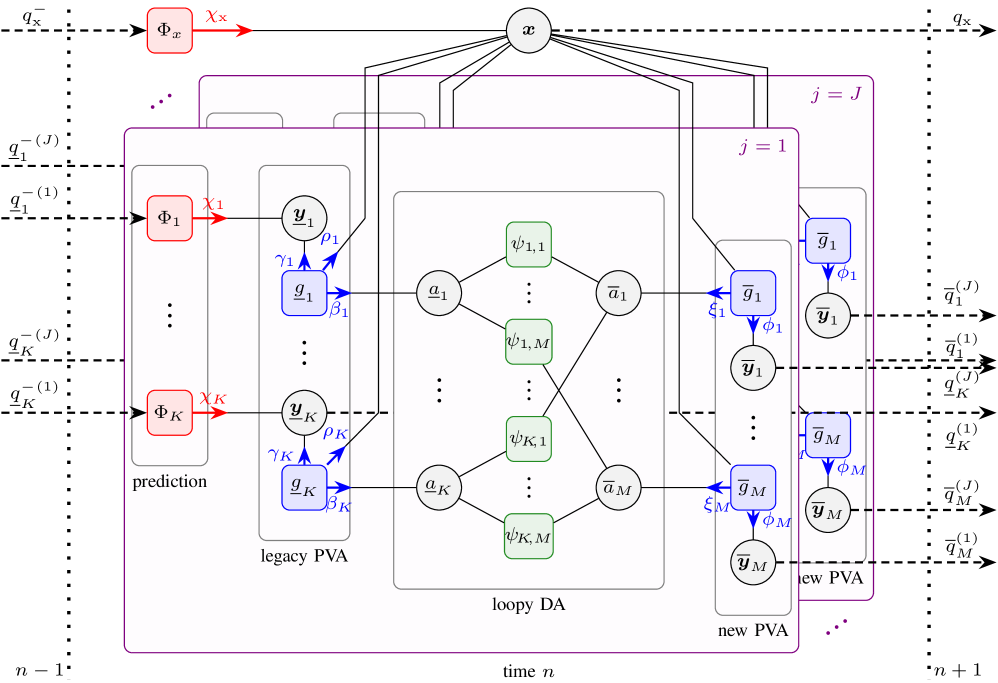
(a)

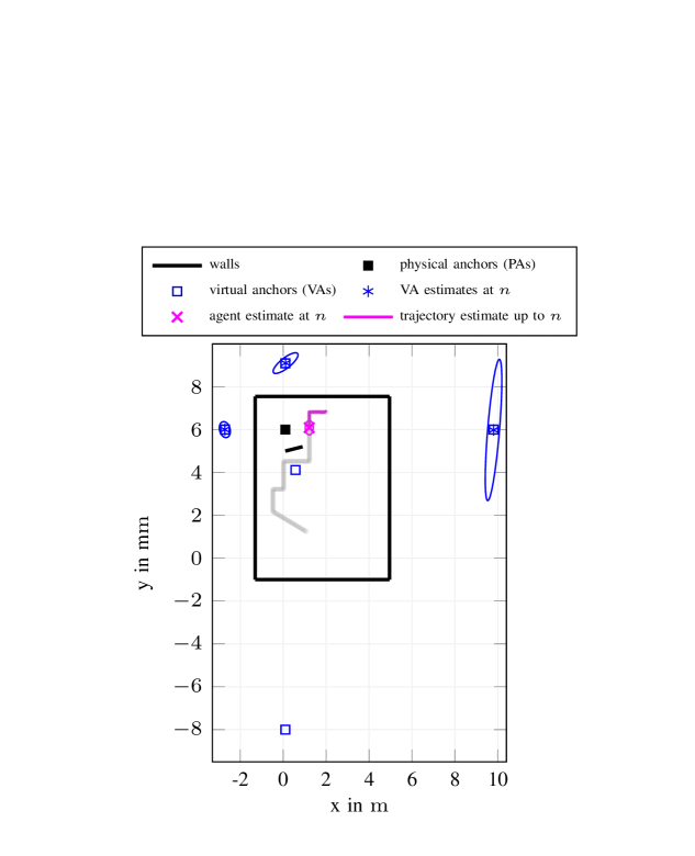
(b)

Figure 2: (a) Factor graph corresponding to the factorization shown in (10). Dashed arrows represent messages that are only passed in one direction. The following short notations are used: $K\triangleq K_{n-1}^{(j)}$, $M\triangleq M_{n}^{(j)}$; variable nodes: $\underline{a}_{k}\triangleq\underline{a}_{k,n}^{(j)}$, $\overline{a}_{m}\triangleq\overline{a}_{m,n}^{(j)}$, $\bm{x}\triangleq\bm{x}_{n}$, $\underline{\bm{y}}_{k}\triangleq\underline{\bm{y}}_{k,n}^{(j)}$, $\overline{\bm{y}}_{m}\triangleq\overline{\bm{y}}_{m,n}^{(j)}$; $\underline{r}_{0}\triangleq\underline{r}_{0,n}^{(j)}$; factor nodes: $\Phi_{x}\triangleq\Phi_{x}(\bm{x}_{n}|\bm{x}_{n})$, $\Phi_{k}\triangleq\Phi_{k}(\underline{\bm{y}}_{k,n}^{(j)}|\bm{y}_{k,n-1}^{(j)})$, $\underline{g}_{k}\triangleq\underline{g}(\bm{x}_{n},\underline{\bm{\psi}}^{(j)}_{k,n},\underline{r}^{(j)}_{k,n},\underline{a}^{(j)}_{k,n};\bm{z}^{(j)}_{n})$, $\overline{g}_{m}\triangleq\overline{g}(\bm{x}_{n},\overline{\bm{\psi}}^{(j)}_{m,n},\overline{r}^{(j)}_{m,n},\overline{a}^{(j)}_{m,n};\bm{z}^{(j)}_{n})$, $\psi_{k,m}\triangleq\psi(\underline{a}_{k,n}^{(j)},\overline{a}_{m,n}^{(j)})$; prediction: $\chi_{k}\triangleq\chi(\underline{\bm{\psi}}_{k,n}^{(j)},\underline{\mathsfbr{r}}_{k,n}^{(j)})$, $\chi_{\text{x}}\triangleq\chi_{\text{x}}(\bm{x}_{n})$; measurement evaluation: $\beta_{k}\triangleq\beta(\underline{a}_{k,n}^{(j)})$, $\xi_{m}\triangleq\xi(\overline{a}_{m,n}^{(j)})$; loopy DA: $\nu_{m,k}\triangleq\nu_{m\rightarrow k}(\underline{a}_{k,n}^{(j)})$, $\zeta_{k,m}\triangleq\zeta_{k\rightarrow m}(\overline{a}_{m,n}^{(j)})$, $\eta_{k}\triangleq\eta(\underline{a}_{k,n}^{(j)})$, $\varsigma_{m}\triangleq\varsigma(\overline{a}_{m,n}^{(j)})$; measurement update: $\gamma_{k}\triangleq\gamma(\underline{\bm{\psi}}_{k,n}^{(j)},\underline{\mathsfbr{r}}_{k,n}^{(j)})$, $\rho_{k}\triangleq\rho_{k}^{(j)}(\bm{x}_{n})$, $\phi_{m}\triangleq\phi(\overline{\bm{\psi}}^{(j)}_{m,n},\overline{r}_{m,n}^{(j)})$, $\kappa_{m}\triangleq\kappa_{m}^{(j)}(\bm{x}_{n})$; belief calculation: $q_{\mathrm{x}}\triangleq q(\bm{x}_{n}),\underline{q}_{k}^{(j)}\triangleq{q}(\underline{\bm{y}}_{k,n}^{(j)}),\overline{q}_{m}^{(j)}\triangleq{q}(\overline{\bm{y}}_{m,n}^{(j)}),q_{\mathrm{x}}^{-}\triangleq q(\bm{x}_{n\hskip-0.85358pt-\hskip-0.85358pt1}),\underline{q}_{k}^{-(j)}\triangleq{q}(\underline{\bm{y}}_{k,n\hskip-0.85358pt-\hskip-0.85358pt1}^{(j)})$. (b) Scenario used to generate synthetic data showing the true map, i.e. one PA with its VAs, the room and a wall temporarily obstructing the LOS, as well as the estimated agent and VA positions along with a visualization of their covariance matrix (100-fold) at time $n=52$.

V Numerical Evaluation

We apply the proposed algorithm to several different settings and compare it against the performance of a MIMO implementation of particle-based MP-SLAM following [4, 8, 17], using a varying number of particles. For the agent, the positioning error is quantified in terms of the root mean squared error (RMSE) and the empirical cumulative distribution function (eCDF) of the error magnitude $e_{\text{pos}}$, while for VAs we show the mean optimal subpattern assignment (OSPA) with a cut-off parameter of 5 and order of 2 [31] and the cardinality error. Furthermore, we display the Cramèr-Rao Lower Bound (CRLB) [32, 33, 34] as a benchmark and the mean runtime of the algorithm per iteration.

V-A Simulation and Algorithm Parameters

Measurements are generated according to the model described in Sec. III-B and only considering first order reflections. The scenario’s geometry depicted in Fig. 2(b) shows the agent’s $N_{\text{steps}}=300$ step long trajectory through an approximately $6.5\mathrm{m}\times 7.5\mathrm{m}$ sized room, equipped with one physical anchor. The signal is transmitted at $f_{c}=6\mathrm{GHz}$ with a bandwidth of $B=500\mathrm{MHz}$ and a root-raised cosine pulse shape with roll-off factor $\beta=0.6$. The signal power follows a free-space path loss model and is equal to $40\mathrm{dB}$ at one-meter distance with each reflection causing a $3\mathrm{dB}$ attenuation. Receiver and transmitter both have a $3\times 3$ antenna array, each element spaced $d_{\text{ant}}=\frac{\lambda}{4}$ apart. The mean number of false alarms is approximated according to $\mu_{\text{fa}}=2N_{\text{ant}}\cdot{e}^{-\gamma^{2}}$ [23] with a detection threshold of $\gamma=9\mathrm{dB}$, which results in a mean clutter rate of $\mu_{\text{fa}}\approx 5$. All experiments were performed with a total of $500$ realizations, except particle implementations involving $100,000$ and $200,000$ particles, which were performed with $200$ realizations. New PVAs are initialized with a mean number of $\mu_{\text{n}}=0.1$ and distributed uniformly on a disc with radius $d_{\text{max}}=15\mathrm{m}$. The survival probability is set to $p_{s}=0.999$ and the threshold of existence above which a VA is considered detected or lost equals $p_{\text{de}}=0.5$ and $p_{\text{pr}}=10^{-4}$ respectively. The loopy data association performs a maximum of $N_{\text{DA}}=10^{5}$ message passing iterations and the number of samples $P$, used to approximate the distribution of new PVAs is $P=10$. Further, we model the movement of the agent according to the continuous velocity and stochastic acceleration model $\bm{\mathsfbr{x}}_{n}=\bm{A}\bm{\mathsfbr{x}}_{n-1}+\bm{B}\bm{\mathsfbr{w}}_{n}^{\prime}$ detailed in [29, p.  273], where $\bm{\mathsfbr{w}}_{n}^{\prime}$ is a zero mean Gaussian noise process, i.i.d. across $n$, and with covariance matrix ${\sigma_{\text{a}}^{2}}\,\bm{I}_{2}$. Here, ${\sigma_{\text{a}}^{2}}$ denotes the acceleration standard deviation, and the state transition matrices are given as

$$\bm{A}=\begin{bmatrix}1&\Delta T\\ 0&1\\ \end{bmatrix}\otimes\bm{I}_{N_{\text{D}}}\hskip 28.45274pt\text{and}\hskip 28.45274pt\bm{B}=\begin{bmatrix}\frac{\Delta T^{2}}{2}\\ \Delta T\\ \end{bmatrix}\otimes\bm{I}_{N_{\text{D}}}$$

with $\Delta T$ as the observation period, set to $1\mathrm{s}$. The model is rewritten to fit the model in Sec. III-A by setting $\bm{\mathsfbr{w}}_{n}\triangleq\bm{B}\bm{\mathsfbr{w}}_{n}^{\prime}$, where $\bm{\mathsfbr{w}}_{n}$ is still zero mean and i.i.d. across $n$, but with covariance matrix

$$\bm{C}_{\text{x}}=\left[\begin{array}[]{cc}\frac{\Delta T^{4}}{4}&\frac{\Delta T^{3}}{2}\\ \frac{\Delta T^{3}}{2}&\Delta T^{2}\end{array}\right]\otimes\bm{I}_{N_{\mathrm{D}}}\sigma_{\mathrm{a}}^{2}.$$

The velocity state transition noise is chosen to be $\sigma_{\text{a}}^{2}=9\cdot 10^{-4}\mathrm{m/s^{2}}$ in accordance with the boundaries given in [29, p. 274] and the orientation variance to $\sigma_{\text{a}}^{2}=5^{\circ}$. The initial agent state is drawn from a normal distribution centred around the true agent position with standard deviations $\sigma_{\text{p},0}=0.1\mathrm{m}$, $\sigma_{\text{v},0}=0.01\mathrm{m/s}$ and $\sigma_{\kappa,0}=10^{\circ}$ for its position, velocity and orientation. The location of all PAs is assumed to be fixed and known, however for numerical reasons a small regularization noise with variance ${\sigma_{\text{reg}}^{2}}=0.01^{2}\mathrm{m}$ is added to their position.

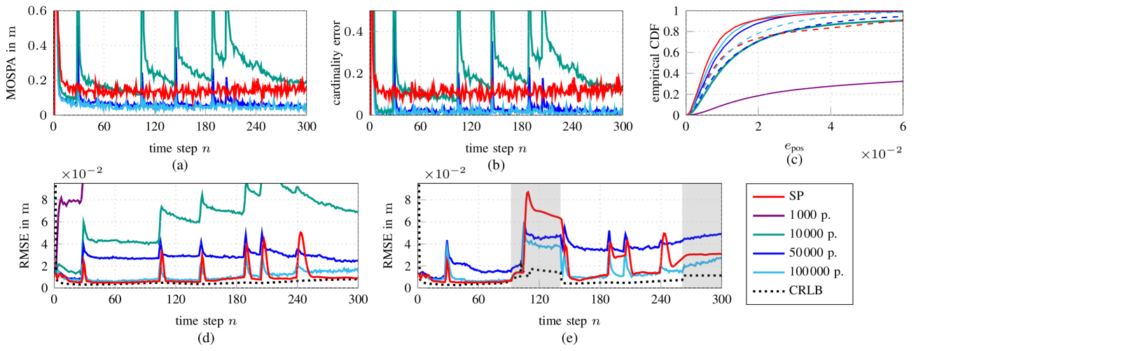
Figure 3: Simulation results in terms of the agent position RMSE from Ex.1 (d) and Ex.2 (e), as well as the mean OSPA of all VAs (a) and associated cardinality error (b) from Ex.1 over all time steps. (c) shows the eCDF of the agent position error for Ex.1 (full) and Ex.2 (dashed). Gray areas in (e) indicate OLOS situations between agent and PA.

V-B Numerical Results

Experiment 1

We consider a scenario, in which the agent and PA have a line-of-sight (LOS) connection throughout the whole trajectory and display the results in Fig. 3a - 3d. The eCDF of the agent’s position error in Fig. 3c and the RMSE in Fig. 3d show similar results for the SP and particle-based implementations with $100\hskip 0.85358pt000$ particles, both of them coming close to the CRLB. The mean OSPA of all VAs (Fig. 3a) is higher for the SP implementation when compared to the $50\hskip 0.85358pt000$ and $100\hskip 0.85358pt000$ particle versions, which can be traced back to a higher mean cardinality error displayed in Fig. 3b. The $10\hskip 0.85358pt000$-particle implementation leads to an agent estimation error larger than $10\mathrm{cm}$ in $8\%$ of cases. The differences in runtime are significant, with the SP version being about $100$ times faster than the comparison algorithm with $100\hskip 0.85358pt000$ particles and around $10$ times faster for $10\hskip 0.85358pt000$ particles. Comparable runtimes could be achieved using $1\hskip 0.85358pt000$ particles, which leads to a total loss of the agent’s trajectory in all $500$ realizations.

TABLE I: Mean runtime per iteration.

SP	1000 p.	10000 p.	50000 p.	100000 p.
$0.029\mathrm{s}$	$0.039\mathrm{s}$	$0.275\mathrm{s}$	$0.948\mathrm{s}$	$1.936\mathrm{s}$

Experiment 2

The overall setting of Ex. 1 is unchanged with an additional wall added to the room, which at times obstructs the LOS connection to the PA as well as to some VAs (Fig. 2(b)). The best result is achieved by the particle-based implementation with $100\hskip 0.85358pt000$ particles, as displayed in Fig. 3 (c) and (e). For the SP implementation the agent position is lost in $1\%$ of realizations, which were removed from the RMSE plot in Fig. 3(e). Execution times remain the same as for Ex. 1 and are listed in Tab. I.

VI Conclusion

We proposed a low complexity implementation of the SPA algorithm for MP-SLAM. By using the uncented or SP transform to approximate PDFs as Gaussian, integrals involved in the SPA can be efficiently evaluated and posterior PDFs accurately represented. This is particularly suitable for MIMO systems, where the joint availability of TOA, AOA and AOD measurements leads to unambiguous transformations, allowing the resulting joint posterior PDF to be approximated accurately by Gaussian densities. Through numerical evaluation in two different MIMO settings, we demonstrated that the proposed algorithm achieves accurate and robust localization results with runtimes in the order of tens of milliseconds. In comparison, a particle-based MP-SLAM algorithm required a high number of particles to achieve similar localization performance, resulting in significantly increased runtimes.

VII Appendix

This appendix provides approximation results for all messages displayed in Fig. 2(a).

Prediction

Applying the agent state transition model stated in Sec. III-A gives

$$\tilde{\chi}_{\text{x}}(\bm{x}_{n})=f_{\text{N}}(\bm{x}_{n};\;\bm{\hat{x}}_{n}^{-},\bm{P}_{n}^{-})\hskip 11.38109pt\text{with}$$

$$\bm{\hat{x}}_{n}^{-}=\bm{A}\bm{\hat{x}}_{n-1},\hskip 14.22636pt\bm{P}_{n}^{-}=\bm{A}\bm{P}_{n-1}\bm{A}^{T}+\bm{C}_{\text{x}}.$$ (25)

PVAs are affected by the survival probability $p_{s}$ as

$$\tilde{\chi}\big{(}\underline{\bm{\psi}}_{k,n}^{(j)}\hskip 0.85358pt,1\big{)}=p_{\mathrm{s}}e_{k,n-1}^{(j)}f_{N}(\underline{\bm{\psi}}_{k,n}^{(j)};\;\underline{\hat{\bm{\psi}}}_{k,n}^{(j)-},\underline{\bm{Q}}_{k,n}^{(j)-})$$ (26)

with $\underline{\hat{\bm{\psi}}}_{k,n}^{(j)-}\hskip-0.85358pt=\hskip-0.85358pt\underline{\hat{\bm{\psi}}}_{k,n-1}^{(j)}$, $\underline{\bm{Q}}_{k,n}^{(j)-}\hskip-0.85358pt=\hskip-0.85358pt\underline{\bm{Q}}_{k,n-1}^{(j)}$ and $e_{k,n-1}^{(j)}$ denoting the existence probability of time $n-1$ calculated in (VII).

Measurement Evaluation legacy PVAs

In the case $\underline{a}_{k,n}^{(j)}=0$ the message equals $\tilde{\beta}\big{(}\underline{a}_{k,n}^{(j)}\big{)}=(1-p_{\text{d}})\chi_{k,n}^{(j)}$ with $\chi_{k,n}^{(j)}=(1-p_{s}e_{k,n-1}^{(j)})$ and otherwise

$$\tilde{\beta}\big{(}\underline{a}_{k,n}^{(j)}\big{)}=\frac{p_{\mathrm{s}}p_{\text{d}}e_{k,n-1}^{(j)}}{\mu_{\mathrm{fa}}f_{\mathrm{fa}}(\bm{z}_{m,n}^{(j)})}f_{\text{N}}(\bm{z}_{m,n}^{(j)};\;\underline{\bm{\mu}}_{k,n}^{(j)},\;\bm{C}_{\text{z}}+\underline{\bm{C}}_{k,n}^{(j)})$$ (27)

where the normal PDF corresponds to $\tilde{\beta}_{\text{part}}\big{(}\underline{a}_{k,n}^{(j)}\big{)}$ in (19).

Measurement Evaluation new PVAs

$$\tilde{\xi}\big{(}\overline{a}^{(j)}_{m,n}\big{)} \approx 1+\frac{{\mu}_{\mathrm{n}}}{\mu_{\mathrm{fa}}\hskip 0.85358ptf_{\mathrm{fa}}(\bm{z}_{m,n}^{(j)})}$$

$$\times\sum^{P}_{p=0}w_{m,n,p}^{(j)}f_{\text{N}}(\bm{z}_{m,n}^{(j)};\;\overline{\bm{\mu}}_{m,n}^{(j)},\;\bm{C}_{\text{z}}+\overline{\bm{C}}_{m,n}^{(j)})$$ (28)

where the computation of $f_{\text{N}}(\cdot)$ and $w_{m,n,p}^{(j)}$ is discussed in Sec. (IV-E).

Loopy Data Association

Messages $\tilde{\beta}\big{(}\underline{a}_{k,n}^{(j)}\big{)}$ and $\tilde{\xi}\big{(}\overline{a}^{(j)}_{m,n}\big{)}$ are fed into the loopy data association, which, after converging, outputs $\tilde{\eta}\big{(}\underline{a}_{k,n}^{(j)}\big{)}$ and $\tilde{\varsigma}\big{(}\overline{a}_{m,n}^{(j)}\big{)}$ according to [25].

Agent Belief

$$\vskip-2.84526pt\tilde{q}(\bm{x}_{n}) =\prod_{j=1}^{J}\prod_{k\in{\cal{K}}_{n-1}^{(j)}}f_{\text{N}}(\bm{x}_{n};\;\bm{\hat{x}}_{k,n}^{(j)}\bm{P}_{k,n}^{(j)}),$$

$$\propto f_{\text{N}}(\bm{x}_{n};\;\bm{\hat{x}}_{n},\bm{P}_{n})$$ (29)

where we refer to Sec. IV-E for a detailed explanation of all terms involved.

Legacy PVAs belief

$$\tilde{q}\big{(}\underline{\bm{\psi}}_{k,n}^{(j)},1\big{)} =p_{\mathrm{s}}e_{k,n-1}^{(j)}f_{\text{N}}(\underline{\bm{\psi}}_{k,n}^{(j)};\;\underline{\hat{\bm{\psi}}}_{k,n}^{(j)-},\underline{\bm{Q}}_{k,n}^{(j)-})\tilde{\eta}\big{(}\underline{a}_{k,n}^{(j)}\!\hskip-0.85358pt=\!0\big{)}$$

$$\times(1\!-\hskip-0.85358ptp_{\text{d}}\hskip 0.85358pt)+\frac{p_{\text{d}}p_{\mathrm{s}}e_{k,n-1}^{(j)}}{\mu_{\mathrm{fa}}\hskip 0.85358ptf_{\mathrm{fa}}(\bm{z}_{m,n}^{(j)})}\sum^{M_{n}^{(j)}}_{\underline{a}_{k,n}^{(j)}=1}\!\!\tilde{\eta}\big{(}\underline{a}_{k,n}^{(j)}\big{)}$$

$$\times\tilde{\beta}_{\text{part}}(\underline{a}_{k,n}^{(j)})f_{\text{N}}(\underline{\bm{\psi}}_{k,n}^{(j)};\;\underline{\hat{\bm{\psi}}^{\prime}}_{k,n}^{(j)},\underline{\bm{Q}^{\prime}}_{k,n}^{(j)})$$

$$\approx e_{k,n}^{(j)}f_{\text{N}}(\underline{\bm{\psi}}_{k,n}^{(j)};\;\underline{\hat{\bm{\psi}}}_{k,n}^{(j)},\underline{\bm{Q}}_{k,n}^{(j)}).$$ (30)

where $\underline{\hat{\bm{\psi}}^{\prime}}_{k,n}^{(j)}$ and $\underline{\bm{Q}^{\prime}}_{k,n}^{(j)}$ result from the KF update, the partial result $\tilde{\beta}_{\text{part}}(\underline{a}_{k,n}^{(j)})$ is given in (19) and the sum is approximated according to [29, p. 55].

New PVAs belief

The measurement update isn’t applied, instead the proposal density from Sec. IV-C is used as distribution for all new PVAs.

Existence of legacy PVAs

$$\vskip-2.84526pte_{k,n}^{(j)} =p_{\mathrm{s}}e_{k,n-1}^{(j)}\tilde{\eta}\big{(}\underline{a}_{k,n}^{(j)}\!\hskip-0.85358pt=\!0\big{)}(1\!-\hskip-0.85358ptp_{\text{d}}\hskip 0.85358pt)+\frac{p_{\mathrm{s}}e_{k,n-1}^{(j)}p_{\text{d}}\hskip 0.85358pt}{\mu_{\mathrm{fa}}\hskip 0.85358ptf_{\mathrm{fa}}(\bm{z}_{m,n}^{(j)})}$$

$$\times\hskip-0.85358pt\hskip-0.85358pt\sum^{M_{n}^{(j)}}_{\underline{a}_{k,n}^{(j)}=1}\!\!\tilde{\eta}\big{(}\underline{a}_{k,n}^{(j)}\big{)}f_{\text{N}}(\bm{z}_{m,n}^{(j)};\;\underline{\bm{\mu}}_{k,n}^{(j)},\;\bm{C}_{\text{z}}+\underline{\bm{C}}_{k,n}^{(j)})$$ (31)

where $f_{\text{N}}(\cdot)$ is the same as in (19) and the sum is again approximated according to [29, p. 55].

Existence of new PVAs

$$\vskip-2.84526pte_{m,n}^{(j)} =\tilde{\varsigma}\big{(}\overline{a}_{m,n}^{(j)}\!\hskip-0.85358pt=\!0\big{)}\frac{\mu_{\mathrm{n}}}{\mu_{\mathrm{fa}}\hskip 0.85358ptf_{\mathrm{fa}}(\bm{z}_{m,n}^{(j)})}$$

$$\times f_{\text{N}}(\bm{z}_{m,n}^{(j)};\;\overline{\bm{\mu}}_{m,n}^{(j)},\;\bm{C}_{\text{z}}+\overline{\bm{C}}_{m,n}^{(j)})+\phi^{(j)}_{m,n}$$ (32)

with $f_{\text{N}}(\cdot)$ given in (18) and $\phi_{m,n}^{(j)}\triangleq\hskip 0.85358pt\tilde{\phi}\big{(}\overline{\bm{\psi}}^{(j)}_{m,n},0\big{)}=\hskip-0.85358pt\sum^{K_{n-1}^{(j)}}_{\overline{a}_{m,n}^{(j)}=0}\!\!\tilde{\varsigma}\big{(}\overline{a}_{m,n}^{(j)}\big{)}$.

References

- [1] K. Witrisal, P. Meissner, E. Leitinger, Y. Shen, C. Gustafson, F. Tufvesson, K. Haneda, D. Dardari, A. F. Molisch, A. Conti, and M. Z. Win, “High-accuracy localization for assisted living: 5G systems will turn multipath channels from foe to friend,” IEEE Signal Process. Mag., vol. 33, no. 2, pp. 59–70, Mar. 2016.
- [2] C. Gentner, T. Jost, W. Wang, S. Zhang, A. Dammann, and U. C. Fiebig, “Multipath assisted positioning with simultaneous localization and mapping,” IEEE Trans. Wireless Commun., vol. 15, no. 9, pp. 6104–6117, Sept. 2016.
- [3] H. Kim, K. Granström, L. Svensson, S. Kim, and H. Wymeersch, “PMBM-based SLAM filters in 5G mmWave vehicular networks,” IEEE Trans. Veh. Technol., pp. 1–1, May 2022.
- [4] E. Leitinger, F. Meyer, F. Hlawatsch, K. Witrisal, F. Tufvesson, and M. Z. Win, “A belief propagation algorithm for multipath-based SLAM,” IEEE Trans. Wireless Commun., vol. 18, no. 12, pp. 5613–5629, Dec. 2019.
- [5] E. Leitinger, A. Venus, B. Teague, and F. Meyer, “Data fusion for multipath-based SLAM: Combining information from multiple propagation paths,” IEEE Trans. Signal Process., vol. 71, pp. 4011–4028, Sep. 2023.
- [6] M. Montemerlo, S. Thrun, D. Koller, and B. Wegbreit, “FastSLAM: A factored solution to the simultaneous localization and mapping problem,” in Proc. AAAI-02, Edmonton, Canda, Jul. 2002, pp. 593–598.
- [7] H. Durrant-Whyte and T. Bailey, “Simultaneous localization and mapping: Part I,” IEEE Robot. Autom. Mag., vol. 13, no. 2, pp. 99–110, Jun. 2006.
- [8] E. Leitinger, S. Grebien, and K. Witrisal, “Multipath-based SLAM exploiting AoA and amplitude information,” in Proc. IEEE ICCW-19, Shanghai, China, May 2019, pp. 1–7.
- [9] R. Mendrzik, F. Meyer, G. Bauch, and M. Z. Win, “Enabling situational awareness in millimeter wave massive MIMO systems,” IEEE J. Sel. Topics Signal Process., vol. 13, no. 5, pp. 1196–1211, Sep. 2019.
- [10] H. Kim, K. Granström, L. Gao, G. Battistelli, S. Kim, and H. Wymeersch, “5G mmWave cooperative positioning and mapping using multi-model PHD filter and map fusion,” IEEE Trans. Wireless Commun., vol. 19, no. 6, pp. 3782–3795, Mar. 2020.
- [11] X. Li, X. Cai, E. Leitinger, and F. Tufvesson, “A belief propagation algorithm for multipath-based SLAM with multiple map features: A mmwave MIMO application,” in Proc. IEEE ICC 2024, Aug. 2024, pp. 269–275.
- [12] L. Wielandner, A. Venus, T. Wilding, K. Witrisal, and E. Leitinger, “MIMO multipath-based SLAM for non-ideal reflective surfaces,” in Proc. Fusion-2024, Venice, Italy, Jul. 2024.
- [13] M. S. Arulampalam, S. Maskell, N. Gordon, and T. Clapp, “A tutorial on particle filters for online nonlinear/non-Gaussian Bayesian tracking,” IEEE Trans. Signal Process., vol. 50, no. 2, pp. 174–188, Feb. 2002.
- [14] S. J. Julier and J. K. Uhlmann, “Unscented filtering and nonlinear estimation,” Proc. IEEE, vol. 92, no. 3, pp. 401–422, Mar. 2004.
- [15] I. Arasaratnam and S. Haykin, “Cubature Kalman filters,” IEEE Trans. Autom. Control, vol. 54, no. 6, pp. 1254–1269, 2009.
- [16] F. Meyer, O. Hlinka, and F. Hlawatsch, “Sigma point belief propagation,” IEEE Signal Process. Lett., vol. 21, no. 2, pp. 145–149, 2014.
- [17] E. Leitinger, L. Wielandner, A. Venus, and K. Witrisal, “Multipath-based SLAM with cooperation and map fusion in MIMO systems,” in Proc. Asilomar-24, Pacifc Grove, CA, USA, Oct. 2024.
- [18] T. L. Hansen, M. A. Badiu, B. H. Fleury, and B. D. Rao, “A sparse Bayesian learning algorithm with dictionary parameter estimation,” in Proc. IEEE SAM-14, 2014, pp. 385–388.
- [19] T. L. Hansen, B. H. Fleury, and B. D. Rao, “Superfast line spectral estimation,” IEEE Trans. Signal Process., vol. PP, no. 99, pp. 2511 – 2526, Feb. 2018.
- [20] S. Grebien, E. Leitinger, K. Witrisal, and B. H. Fleury, “Super-resolution estimation of UWB channels including the dense component – An SBL-inspired approach,” IEEE Trans. Wireless Commun., vol. 23, no. 8, pp. 10 301–10 318, Feb. 2024.
- [21] J. Möderl, A. M. Westerkam, and E. Leitinger, “A block-sparse Bayesian learning algorithm with dictionary parameter estimation for multi-sensor data fusion,” submitted to Fusion 2025, Jul. 7–11, 2025, Rio de Janeiro, Brazil.
- [22] X. Li, E. Leitinger, A. Venus, and F. Tufvesson, “Sequential detection and estimation of multipath channel parameters using belief propagation,” IEEE Trans. Wireless Commun., pp. 1–1, Apr. 2022.
- [23] A. Venus, E. Leitinger, S. Tertinek, F. Meyer, and K. Witrisal, “Graph-based simultaneous localization and bias tracking,” IEEE Trans. Wireless Commun., vol. 23, no. 10, pp. 13 141–13 158, May 2024.
- [24] F. Meyer, T. Kropfreiter, J. L. Williams, R. Lau, F. Hlawatsch, P. Braca, and M. Z. Win, “Message passing algorithms for scalable multitarget tracking,” Proc. IEEE, vol. 106, no. 2, pp. 221–259, Feb. 2018.
- [25] J. Williams and R. Lau, “Approximate evaluation of marginal association probabilities with belief propagation,” IEEE Trans. Aerosp. Electron. Syst., vol. 50, no. 4, pp. 2942–2959, Oct. 2014.
- [26] S. M. Kay, Fundamentals of Statistical Signal Processing: Estimation Theory. Upper Saddle River, NJ, USA: Prentice Hall, 1993.
- [27] F. Kschischang, B. Frey, and H.-A. Loeliger, “Factor graphs and the sum-product algorithm,” IEEE Trans. Inf. Theory, vol. 47, no. 2, pp. 498–519, Feb. 2001.
- [28] H.-A. Loeliger, “An introduction to factor graphs,” IEEE Signal Process. Mag., vol. 21, no. 1, pp. 28–41, Feb. 2004.
- [29] Y. Bar-Shalom, T. Kirubarajan, and X.-R. Li, Estimation with Applications to Tracking and Navigation. New York, NY, USA: John Wiley & Sons, Inc., 2002.
- [30] P. Bromiley, “Products and convolutions of Gaussian probability density functions,” 2003. [Online]. Available: leimao.github.io
- [31] D. Schuhmacher, B.-T. Vo, and B.-N. Vo, “A consistent metric for performance evaluation of multi-object filters,” IEEE Trans. Signal Process., vol. 56, no. 8, pp. 3447–3457, Aug. 2008.
- [32] P. Tichavsky, C. Muravchik, and A. Nehorai, “Posterior cramer-rao bounds for discrete-time nonlinear filtering,” IEEE Trans. Signal Process., vol. 46, no. 5, pp. 1386–1396, May 1998.
- [33] E. Leitinger, P. Meissner, C. Rudisser, G. Dumphart, and K. Witrisal, “Evaluation of position-related information in multipath components for indoor positioning,” IEEE J. Sel. Areas Commun., vol. 33, no. 11, pp. 2313–2328, Nov. 2015.
- [34] O. Kaltiokallio, Y. Ge, J. Talvitie, H. Wymeersch, and M. Valkama, “mmWave simultaneous localization and mapping using a computationally efficient EK-PHD filter,” in Proc. IEEE Fusion 2021, Nov. 2021, pp. 1–8.