Polynomial and Parallelizable Preconditioning
for Block Tridiagonal Positive Definite Matrix

Abstract

The efficient solution of moderately large-scale linear systems arising from the KKT conditions in optimal control problems (OCPs) is a critical challenge in robotics. With the stagnation of Moore’s law, there is growing interest in leveraging GPU-accelerated iterative methods, and corresponding parallel preconditioners, to overcome these computational challenges. To improve the computational performance of such solvers, we introduce a parallel-friendly, parametrized multi-splitting polynomial preconditioner framework that leverages positive and negative factors. Our approach results in improved convergence of the linear systems solves needed in OCPs. We construct and prove the optimal parametrization of multi-splitting theoretically and demonstrate empirically a 76% reduction in condition number and 46% in iteration counts on a series of numerical benchmarks.

I Introduction

The efficient solution of moderately large-scale linear systems arising from the Karush-Kuhn-Tucker (KKT) conditions in optimal control problems (OCPs) is a fundamental challenge in model predictive control (MPC) and trajectory optimization [1]. These problems are central to enabling real-time, high-performance robotic behaviors in tasks ranging from locomotion to manipulation [2, 3, 4, 5, 6]. The structure of these systems, typically characterized by a block tridiagonal positive definite matrix due to stage-wise equality constraints, makes direct factorization computationally prohibitive for large problem instances. This necessitates the development of custom solvers optimized for scalable efficiency on their target computational platforms [7, 8].

At the same, as Moore’s law slows and traditional CPU performance scaling stagnates [9, 10], interest in acceleration on parallel computational hardware, such as GPUs, has greatly increased. As a result, iterative methods, particularly the Conjugate Gradient (CG) algorithm [11], have grown in popularity as they are well-suited for parallel computation [12, 13]. However, the performance of these iterative solvers is strongly dependent on the choice of numerical preconditioners, which are essential for both the convergence and the computational efficiency of the algorithm [14].

Unfortunately, many popular preconditioners place limitations on the underlying matrix structure and as such only support specific classes of problems. For example, block-structure preconditioners may require non-negativity of off-diagonal entries (M-matrix) [15], or diagonal dominance [16], or specific sparsity patterns (e.g. Toeplitz structure [17]). For the structured KKT matrices arising from OCPs, none of these properties hold. Similarly, many standard preconditioning techniques based on optimization methods (e.g. SDP) [18] and block incomplete factorization [15, 16] are not inherently parallel-friendly, limiting their effectiveness in GPU-accelerated and distributed computing settings.

To address these challenges, we propose a novel polynomial preconditioner tailored for symmetric positive definite block tridiagonal matrices, which frequently arise in OCPs [7, 19]. Our approach emphasizes parallelizability, making it well-suited for GPU-accelerated and large-scale robotics applications. Our framework constructs a parametrized multi-splitting family of preconditioners that retain computational efficiency while enabling inherent parallelism. The key contributions of this work include: (1) the development of a parametrized family of polynomial preconditioners; (2) a rigorous analysis of their convergence properties; and (3) a demonstration of their effectiveness through numerical experiments. Overall we prove that a multi-splitting using both positive and negative factors qualifies for preconditioning and construct an optimal splitting which is able to halve the number of distinct eigenvalues and numerically reduce the condition number and resulting solver iteration counts by as much as 76% and 46% respectively on a series of numerical benchmarks as compared with the state-of-the-art [19].

II Preliminaries

II-A Symmetric positive definite block tridiagonal matrix

We focus on s.p.d. block tridiagonal matrices $A\in S^{Nn}_{++}$, where $N$ denotes the number of diagonal blocks and $n$ denotes the block size. $N=3$ will be used throughout the paper:

$$A=\begin{bmatrix}D_{1}&O_{1}&\\ O_{1}^{\mathrm{T}}&D_{2}&O_{2}\\ &O_{2}^{\mathrm{T}}&D_{3}\end{bmatrix},\quad D_{k},O_{k}\in\mathbb{R}^{n\times n}.$$ (1)

An immediate result of $A\in S^{Nn}_{++}$ is $D_{k}\in S_{++}^{n},\forall k$. No assumption is placed towards sparsity of $D_{k},O_{k}$, i.e., they are viewed as general dense blocks with $n^{2}$ entries each.

II-B Matrix splittings and polynomial preconditioning

Many preconditioners arise from matrix splittings. In this section, we review the definitions and properties of so-called P-regular splittings and their connections to multi-splittings:

Definition 2.1.

[20] Let $A,B,C\in\mathbb{R}^{n\times n}$. $A=B-C$ is a P-regular splitting of $A$ if $B$ is nonsingular and $B+C$ is p.d.

Lemma 2.1.

[20] If $A\in\mathbb{R}^{n\times n}$ is s.p.d and $A=B-C$ is a P-regular splitting, then $\rho(B^{-1}C)<1$.

Definition 2.2.

[21] Let $A,B_{k},C_{k},D_{k}\in\mathbb{R}^{n\times n}$. $(B_{k},C_{k},D_{k})$ is called a multi-splitting of $A$ if

• $A=B_{k}-C_{k},k=1,\dots,K$ with each $B_{k}$ invertible.

• $\sum_{k=1}^{K}D_{k}=I$ with each $D_{k}$ diagonal and $D_{k}\geq 0$.

Given a multi-splitting, we construct the notations

$$H \coloneqq\sum_{k=1}^{K}D_{k}B_{k}^{-1}C_{k} G \coloneqq\sum_{k=1}^{K}D_{k}B_{k}^{-1}$$ (2)

Although $G$ and $H$ stem from multi-splitting, they can be interpreted as deriving from a single splitting $A=B-C$

$$B =G^{-1} C =G^{-1}H$$ (3)

Since $B$ and $G$ are invertible, (3) is equivalent to

$$G =B^{-1} H =B^{-1}C$$ (4)

Lemma 2.2.

[21] If $(B_{k},C_{k})$ is a P-regular splitting of a s.p.d. matrix $A$ and $D_{k}=\alpha_{k}I$, $\forall k$, then $\rho(H)<1$.

The introduction of P-regular splitting with $\rho(B^{-1}C)<1$ and multi-splitting composed with P-regular splittings $\rho(H)<1$, both of which are convergent [14], is justified.

Lemma 2.3.

[22][Neumann series] If $A,B,C\in\mathbb{R}^{n\times n}$, $A,B$ are nonsingular, $A=B-C$ and $\rho(B^{-1}C)<1$, then with (4),

$$\lim_{k\rightarrow\infty}\Big{(}I+H+H^{2}+\dots+H^{k}\Big{)}G=A^{-1}$$ (5)

Definition 2.3.

[23][Truncated Neumann series] Under the same conditions as Lemma 2.3, to approximate $A$, the $m$-step polynomial preconditioner $M_{m}$ is defined as:

$$M_{m}\coloneqq G^{-1}(I+H+H^{2}+\dots+H^{m-1})^{-1}$$ (6)

In this paper, the inverse of (6) is used more frequently:

$$M_{m}^{-1}=(I+H+H^{2}+\dots+H^{m-1})G$$ (7)

While convergence of the splitting is needed, it is insufficient for $M_{m}$ to be a s.p.d. preconditioner for the CG method. As such, we present two more lemmas to fill that gap:

Lemma 2.4.

[23] If $A=B-C$ is s.p.d. and $B$ is symmetric and nonsingular, then with (4),

1. $M_{m}$ is symmetric.

2. For $m$ odd, $M_{m}$ is p.d. if and only if $B$ is p.d.

3. For $m$ even, $M_{m}$ is p.d. if and only if $B+C$ is p.d.

Lemma 2.5.

[23][Continuation of Lemma 2.1] Under the same conditions as Lemma 2.4, $\rho(B^{-1}C)<1$ if and only if $B+C$ is p.d.

II-C Splittings of s.p.d. block tridiagonal matrix

In this section, we examine two fundamental types of parallel-friendly splittings of $A$ in (1), which serve as the basis for both multi-splittings and polynomial preconditioner.

II-C1 Diagonal splitting

The diagonal splitting $A=B_{d}-C_{d}$ is defined as:

$$B_{d}=\begin{bmatrix}D_{1}&\\ &D_{2}&\\ &&D_{3}\end{bmatrix}\mkern 9.0muC_{d}=\begin{bmatrix}0&-O_{1}&\\ -O_{1}^{\mathrm{T}}&0&-O_{2}\\ &-O_{2}^{\mathrm{T}}&0\end{bmatrix}$$ (8)

Lemma 2.6.

The diagonal splitting is P-regular.

Proof.

$B_{d}$ is s.p.d. and thus invertible. $B_{d}+C_{d}$ is symmetric so it suffices to prove it is p.d. $A$ is s.p.d $\Rightarrow\forall x=\begin{bmatrix}x_{1}^{\mathrm{T}}&x_{2}^{\mathrm{T}}&x_{3}^{\mathrm{T}}\end{bmatrix}^{\mathrm{T}}\neq 0,x^{\mathrm{T}}Ax>0$. Given $x$, define two vectors $x_{e}=\begin{bmatrix}x_{1}^{\mathrm{T}}&-x_{2}^{\mathrm{T}}&x_{3}^{\mathrm{T}}\end{bmatrix}^{\mathrm{T}}$ and $x_{o}=\begin{bmatrix}-x_{1}^{\mathrm{T}}&x_{2}^{\mathrm{T}}&-x_{3}^{\mathrm{T}}\end{bmatrix}^{\mathrm{T}}$. By construction, $x^{\mathrm{T}}Ax=x_{e}^{\mathrm{T}}(B_{d}+C_{d})x_{e}=x_{o}^{\mathrm{T}}(B_{d}+C_{d})x_{o}>0,\forall x,x_{e},x_{o}$. The deduction generalizes to all $N$. ∎

II-C2 Stair splittings

The left and right stair splittings $A=B_{l}-C_{l}=B_{r}-C_{r}$ are defined as:

$$B_{l} =\begin{bmatrix}D_{1}&&\\ O_{1}^{\mathrm{T}}&D_{2}&O_{2}\\ &&D_{3}\end{bmatrix}\mkern 9.0muC_{l}=\begin{bmatrix}0&-O_{1}&\\ &0&\\ &-O_{2}^{\mathrm{T}}&0\end{bmatrix}$$ (9)

$$B_{r} =\begin{bmatrix}D_{1}&O_{1}&\\ &D_{2}&\\ &O_{2}^{\mathrm{T}}&D_{3}\end{bmatrix}\mkern 9.0muC_{r}=\begin{bmatrix}0&&\\ -O_{1}^{\mathrm{T}}&0&-O_{2}\\ &&0\end{bmatrix}$$

Lemma 2.7.

The left and right stair splittings are P-regular.

Proof.

$B_{l},B_{r}$ are invertible because they contain all the diagonal s.p.d. blocks. $sym(B_{l}+C_{l})=sym(B_{r}+C_{r})=B_{d}$, which is s.p.d., holds by construction. ∎

Remark 2.1.

[24] The inverse of $B_{l}$ and $B_{r}$ are still in respective stair shapes and parallel-friendly to compute. The diagonal blocks of $B_{l}^{-1}$ and $B_{r}^{-1}$ are $D_{i}^{-1}$. The off-diagonal blocks w.r.t. $O_{i}$ only involve consecutive $D_{i}^{-1}$ and $D_{i+1}^{-1}$.

Due to the sparsity pattern of $B_{l}$ and $B_{r}$, we introduce the following notation to discuss their eigenvalues. For $v^{\mathrm{T}}=(v_{1}^{\mathrm{T}},v_{2}^{\mathrm{T}},\dots,v_{i}^{\mathrm{T}},\dots,v_{N}^{\mathrm{T}})\in\mathbb{R}^{Nn}$ and $v_{i}\in\mathbb{R}^{n}$, denote $v_{e}^{\mathrm{T}}=(0,v_{2}^{\mathrm{T}},\dots,0,v_{2j}^{\mathrm{T}},\dots)$ and $v_{o}^{\mathrm{T}}=(v_{1}^{\mathrm{T}},0,\dots,v_{2j+1}^{\mathrm{T}},0,\dots)$ such that $v=v_{e}+v_{o}$.

III m-step preconditioners from multi-splitting

In this section, we construct a family of parametric multi-splittings from diagonal splitting (8) and stair splittings (9), prove their properties if viewed as single splittings, and extend the single splittings to $m$-step preconditioners (6) or its inverse (7). Finally, we discuss how the choice of parameters influences the quality of the resulting preconditioners.

III-A Parametric multi-splitting family

Following Definition 2.2, a family of multi-splittings is constructed with $(B_{k},C_{k},D_{k}),k\in\{d,l,r\},K=3$ and $D_{l}=D_{r}=aI,D_{d}=bI$ where $(a,b)\in\mathcal{C}$

$$\mathcal{C}=\{a,b\in\mathbb{R}\mid 2a+b=1\}$$ (10)

Mimicking (2), the corresponding family of matrices $(G_{ab},H_{ab})$ is defined as

$$G_{ab} \coloneqq a(B_{l}^{-1}+B_{r}^{-1})+bB_{d}^{-1}$$ (11)

$$H_{ab} \coloneqq a(B_{l}^{-1}C_{l}+B_{r}^{-1}C_{r})+bB_{d}^{-1}C_{d}$$

By construction, $G_{ab}$ is symmetric and $G_{ab}A+H_{ab}=I,\forall(a,b)\in\mathcal{C}$. So if $(\lambda,v)$ is an eigenpair of $G_{ab}A$, $(1-\lambda,v)$ will be an eigenpair of $H_{ab}$. The same statement holds in the opposite direction.

Motivated by (3), $G_{ab}$ and $H_{ab}$ can be interpreted as deriving from a single splitting $A=B_{ab}-C_{ab}$

$$B_{ab} \coloneqq G_{ab}^{-1} C_{ab} \coloneq G_{ab}^{-1}H_{ab}$$ (12)

The inverse of $m$-step preconditioner related to the single splitting (12) is defined as:

$$_{ab}M_{m}^{-1}\coloneqq(I+H_{ab}+H_{ab}^{2}+\dots+H_{ab}^{m-1})G_{ab}$$ (13)

III-B Multi-splitting with nonnegative $a,b$

In this subsection, inspired by the widely-used non-negative weightings in multi-splitting [21], we focus on the set $\mathcal{C}_{+}$, a subset of $\mathcal{C}$:

$$\mathcal{C}_{+}=\{a,b\in\mathbb{R}\mid 2a+b=1,a,b\geq 0\}$$ (14)

Theorem 3.1.

$\forall a,b\in\mathcal{C}_{+}$,

1. $G_{ab}$ is s.p.d.

2. The splitting (12) is convergent, i.e., $\rho(H_{ab})<1$.

3. $\forall m\in\mathbb{N}$, the matrix ${}_{ab}M_{m}^{-1}$ in (13) is s.p.d.

Proof.

Since $B_{l}^{-1}+B_{r}^{-1}$ and $B_{d}^{-1}$ are s.p.d., their non-negatively weighted sum $G_{ab}$ is s.p.d.. Point 2) follows from Lemma 2.2 directly. According to Lemma 2.5, $\rho(H_{ab})<1\Rightarrow B_{ab}+C_{ab}$ is p.d. For $m$ even, Point 3) follows from points 1 & 3 of Lemma 2.4. For $m$ odd, Point 3) follows from points 1 & 2 of Lemma 2.4. ∎

We explore two extreme cases to motivate the generalization of Theorem 3.1 presented in the following subsection.

III-B1 Extreme case $a=0,b=1$

$G_{0,1}$ is block diagonal. $H_{0,1}$ is block tridiagonal.

$$G_{0,1} =B_{d}^{-1} H_{0,1} =B_{d}^{-1}C_{d}$$ (15)

$G_{0,1}$ is the commonly-used block diagonal Jacobi preconditioner. It is the special case of ${}_{0,1}M_{m}^{-1}$ when $m=0$.

Lemma 3.1.

If $(\lambda\neq 0,v=v_{e}+v_{o})$ is an eigenpair of $B_{l}^{-1}C_{l}$,

• $(\pm\sqrt{\lambda},v_{e}\pm\sqrt{\lambda}v_{o})$ are eigenpairs of $H_{0,1}$.

• $(1-(\pm\sqrt{\lambda}),v_{e}\pm\sqrt{\lambda}v_{o})$ are eigenpairs of $G_{0,1}A$.

Proof.

According to [19], $B_{d}^{-1}C_{l}v=B_{d}^{-1}C_{l}v_{e}=\lambda v_{o}$. The counterpart $B_{d}^{-1}C_{r}v=B_{d}^{-1}C_{r}v_{o}=v_{e}$ holds symmetrically.

$$H_{0,1}(\alpha v_{e}+\beta v_{o}) =B_{d}^{-1}C_{d}(\alpha v_{e}+\beta v_{o})$$ (16)

$$=B_{d}^{-1}(C_{l}+C_{r})(\alpha v_{e}+\beta v_{o})$$

$$=\alpha B_{d}^{-1}C_{l}v_{e}+\beta B_{d}^{-1}C_{r}v_{o}$$

$$=\alpha\lambda v_{o}+\beta v_{e}$$

(16) holds iff $\frac{\alpha\lambda}{\beta}=\frac{\beta}{\alpha}\Leftrightarrow\alpha^{2}\lambda=\beta^{2}\Leftrightarrow\beta=\pm\sqrt{\lambda}\alpha$. ∎

Lemma 3.2.

All non-zero eigenvalues of $B_{l}^{-1}C_{l}$ (or equivalently $B_{r}^{-1}C_{r}$) are real and contained in $(0,1)$.

Proof.

$G_{0,1}$ is s.p.d, so $X=G_{0,1}^{\frac{1}{2}}$ is well-defined and s.p.d.. $P=G_{0,1}A$ is similar to the matrix $Q=XAX$ because $X^{-1}PX=Q$, so $P,Q$ has the same sets of eigenvalues. $Q$ is congruent to $A$ so only has positive eigenvalues. Hence all eigenvalues of $P$ are real and positive. $\forall\lambda\in\sigma(B_{l}^{-1}C_{l})$ that are non-zero, $1\pm\sqrt{\lambda}$ are the eigenvalues of $P$ and they are real and positive. As a result, $\lambda\in\mathbb{R}$ and $\lambda\in(0,1)$. ∎

TABLE I: Comparison of ${}_{ab}M_{m}^{-1}$ for different sets of $a,b$

Values of $a,b$		$a=0,b=1$	$a=\frac{1}{2},b=0$	$a=1,b=-1$
unique eigenvalues of $M^{-1}A$		$Nn$	$Nn$	${\color[rgb]{1,0,0}\frac{N}{2}n}$ or ${\color[rgb]{1,0,0}\left\lfloor\frac{N}{2}\right\rfloor n+1}$
$m=1$ $M^{-1}=G$	closed-form	$B_{d}^{-1}$	$\frac{1}{2}(B_{l}^{-1}+B_{r}^{-1})$	$B_{l}^{-1}+B_{r}^{-1}-B_{d}^{-1}$
	shape	block diagonal	block tridiagonal
	$M^{-1}A$ spectrum	$(0,2)$	$(0,\frac{9}{8}]$	$(0,1]$ or $(0,1)$
$m=2$ $M^{-1}=(I+H)G$	closed-form	$B_{d}^{-1}C_{d}$	$\frac{1}{2}(B_{l}^{-1}C_{l}+B_{r}^{-1}C_{r})$	$B_{l}^{-1}C_{l}+B_{r}^{-1}C_{r}-B_{d}^{-1}C_{d}$
	$H$ shape	sparse block tridiagonal	dense block pentadiagonal	(checkerboard) sparse block pentadiagonal
	shape	block tridiagonal	block heptadiagonal
	$M^{-1}A$ spectrum	$(0,1]$

III-B2 Extreme case $a=\frac{1}{2},b=0$

$G_{\frac{1}{2},0}$ is block tridiagonal. $H_{\frac{1}{2},0}$ is block penta-diagonal.

$$G_{\frac{1}{2},0} =\frac{1}{2}(B_{l}^{-1}+B_{r}^{-1}) H_{\frac{1}{2},0} =\frac{1}{2}(B_{l}^{-1}C_{l}+B_{r}^{-1}C_{r})$$ (17)

$G_{\frac{1}{2},0}$ is named as additive stair preconditioner in [19]. It is the special case of ${}_{\frac{1}{2},0}M_{m}^{-1}$ when $m=1$.

Lemma 3.3.

[19] If $(\lambda\neq 0,v=v_{e}+v_{o})$ is an eigenpair of $B_{l}^{-1}C_{l}$, then

• $(\frac{1}{2}(\lambda\pm\sqrt{\lambda}),v_{e}\pm\sqrt{\lambda}v_{o})$ are eigenpairs of $H_{\frac{1}{2},0}$.

• $(1-\frac{1}{2}(\lambda\pm\sqrt{\lambda}),v_{e}\pm\sqrt{\lambda}v_{o})$ are eigenpairs of $G_{\frac{1}{2},0}A$.

III-C Multi-splitting when $a,b$ can be negative

Since Lemma 2.2 only works when all $D_{k}=\alpha_{k}I,\alpha_{k}\geq 0$, the conclusions of Theorem 3.1 might not hold if $a$ or $b$ is negative. In this subsection, we extend Theorem 3.1 to negative $b$ and prove that negative $a$ invalidates the theorem. To the best of author’s knowledge, this is the first time negative weightings are introduced in multi-splitting with guarantees. We conclude the subsection with an optimal pair of $a,b$ in terms of clustered spectrum, CG iteration numbers, and storage usage (Table I).

III-C1 General case

The following theorem generalizes Lemmas 3.1 and 3.3. Let $f_{a}(\lambda)$ denotes $f_{a+}(\lambda)$ or $f_{a-}(\lambda)$, where

$$f_{a\pm}(\lambda) \coloneqq a\lambda\pm(1-a)\sqrt{\lambda}$$ (18)

Lemma 3.4 (Generalization of Lemmas 3.1 and 3.3).

If $(\lambda\neq 0,v=v_{e}+v_{o})$ is an eigenpair of $B_{l}^{-1}C_{l}$,

• $(f_{a+}(\lambda),v_{e}+\sqrt{\lambda}v_{o})$ and $(f_{a-}(\lambda),v_{e}-\sqrt{\lambda}v_{o})$ are eigenpairs of $H_{ab}$.

• $(1-f_{a+}(\lambda),v_{e}+\sqrt{\lambda}v_{o})$ and $(1-f_{a-}(\lambda),v_{e}-\sqrt{\lambda}v_{o})$ are eigenpairs of $G_{ab}A$.

Proof.

Follow similar deduction as in (16). ∎

Denote the maximum eigenvalue of $B_{l}^{-1}C_{l}$ as $\lambda_{max}$. The following theorem shows how $a$ influences the convergence of matrix splitting $A=B_{ab}-C_{ab}$ and the spectrum of $G_{ab}A$.

Lemma 3.5.

[On $\rho(H_{ab})$ and spectrum of $G_{ab}A$]

1. $a\in[0,1]$ is the only condition guarantees $\rho(H_{ab})<1$.

   1. $\rho(H_{ab})=\max(1-2a,f_{a+}(\lambda_{max}))$ if $a\in[0,\frac{1}{3}]$.

   2. $\rho(H_{ab})=\max(\frac{(1-a)^{2}}{4a},f_{a+}(\lambda_{max}))$ if $a\in(\frac{1}{3},1]$.

   3. If $a\in(-\infty,0)\cup(1,\infty)$, there might be some $\lambda\in\sigma(B_{l}^{-1}C_{l})$ that lead to $\rho(H_{ab})>1$.

2. $a\in[-1,1]$ is the only condition that guarantees positive eigenvalues of $G_{ab}A$, i.e. $\mathcal{I}_{G_{ab}A}\subset\mathbb{R}_{>0}$.

   1. If $a\in[-1,\frac{1}{3}]$, then $\mathcal{I}_{G_{ab}A}=(0,2-2a)$.

   2. If $a\in(\frac{1}{3},1]$, then $\mathcal{I}_{G_{ab}A}=(0,\frac{(1-a)^{2}}{4a})$.

   3. If $a\in(-\infty,-1)\cup(1,\infty)$, there might be some $\lambda\in\sigma(B_{l}^{-1}C_{l})$ that leads to negative eigenvalue of $G_{ab}A$.

Proof.

See Appendix -A. ∎

As a result,  12 is convergent and $G_{ab}A$ has positive eigenvalues hold simultaneously only if $a\in[0,1]$. A more general set is defined considering the new restriction on $a$:

$$\mathcal{C}_{g}=\{a,b\in\mathbb{R}\mid 2a+b=1,a\geq 0,{\color[rgb]{1,0,0}b\geq-1}\}$$ (19)

Theorem 3.2.

$\forall(a,b)\in\mathcal{C}_{g}$,

1. $G_{ab}$ is s.p.d.

2. The splitting (12) is convergent, i.e., $\rho(H_{ab})<1$.

3. $\forall m\in\mathbb{N}$, the matrix ${}_{ab}M_{m}^{-1}$ in (13) is s.p.d.

Proof.

According to Lemma 3.5, $(a,b)\in\mathcal{C}_{g}\Rightarrow\rho(H_{ab})<1\Rightarrow B_{ab}+C_{ab}$ is p.d. $(a,b)\in\mathcal{C}_{g}$ also means that all eigenvalues of $X=G_{ab}A$ are real and positive. Then $G_{ab}=XA^{-1}$. Multiplying $G_{ab}$ by $A^{\frac{1}{2}}$ on the left and right, we have $A^{\frac{1}{2}}G_{ab}A^{\frac{1}{2}}=A^{\frac{1}{2}}XA^{-\frac{1}{2}}$. The matrix on the right is similar to $X$ and hence has the same eigenvalues, while the matrix on the left is congruent to $G_{ab}$ and hence has the same number of positive eigenvalues. Thus $G_{ab}$ has the same number of positive eigenvalues as $X$ and so is p.d. The rest of proof is the same as for Theorem 3.1. ∎

Lemma 3.6.

If $\lambda\neq 0$ is an eigenvalue of $B_{l}^{-1}C_{l}$, ${}_{ab}M_{m}^{-1}A$ has a pair of eigenvalues at $1-f_{a+}(\lambda)^{m}$ and $1-f_{a-}(\lambda)^{m}$.

Proof.

According to Lemma 3.4, let $v$ be an eigenvector of $G_{ab}A$ and $H_{ab}$. $\forall j\in\mathbb{N}$:

$$H_{ab}^{j}G_{ab}Av=(1-f_{a}(\lambda))f_{a}(\lambda)^{j}v$$ (20)

Recall the definition of ${}_{ab}M_{m}^{-1}A$ by (13):

$$_{ab}M_{m}^{-1}Av =(I+H_{ab}+H_{ab}^{2}+\dots+H_{ab}^{m-1})G_{ab}Av$$

$$=(1-f_{a}(\lambda))(1+f_{a}(\lambda)+\dots+f_{a}(\lambda)^{m-1})v$$

$$=(1-f_{a}(\lambda)^{m})v$$ (21)

(III-C1) follows from the sum of geometric progression. ∎

Remark 3.1.

Lemma 3.6 explains more intuitively why $\forall(a,b)\in\mathcal{C}_{g}$, larger $m$ generates ${}_{ab}M_{m}^{-1}$ that is closer to $A^{-1}$. The reason is $\forall\lambda\in(0,1),\forall a\in[0,1],f_{a}(\lambda)\in(0,1)\Rightarrow\lim_{m\rightarrow\infty}f_{a}(\lambda)^{m}=0$. Larger $m$ will cause all eigenvalues tend to one, which means ${}_{ab}M_{m}^{-1}A$ tends to the identity matrix. For fixed $m$, the smaller $f_{a}(\lambda)$ is, the better.

III-C2 Optimal case $a=1,b=-1$

$G_{1,-1}$ is block tridiagonal. $H_{1,-1}$ is block penta-diagonal with zero super and sub-diagonal blocks like a checkerboard.

$$G_{1,-1} =B_{l}^{-1}+B_{r}^{-1}-B_{d}^{-1}$$ (22)

$$H_{1,-1} =B_{l}^{-1}C_{l}+B_{r}^{-1}C_{r}-B_{d}^{-1}C_{d}$$

We note that $G_{1,-1}$ is named the symmetric stair preconditioner in [19], where $H_{1,-1}$ was not explicitly defined and positive definiteness of $G_{1,-1}$ was not proved. It is the special case of ${}_{1,-1}M_{m}^{-1}$ when $m=1$.

Remark 3.2.

By inspection, $\forall m\in\mathbb{N},_{1,-1}M_{m}^{-1}=_{0,1}M_{2m}^{-1}$.

Remark 3.3.

[19] If $(\lambda,v=v_{e}+v_{o})$ is an eigenpair of $B_{l}^{-1}C_{l}$, then $(\lambda,v_{o})$ and $(\lambda,v_{e})$ are eigenpairs of $H_{1,-1}$ and $(1-\lambda,v_{o})$ and $(1-\lambda,v_{e})$ are eigenpairs of $G_{1,-1}A$ due to the degeneracy of $f_{a}$ to the identity map. This is a special case of Lemma 3.4

Lemma 3.6 and Remark 3.3 together show that the eigenvalues of ${}_{1,-1}M_{m}^{-1}A$ come in pairs, $\forall m\in\mathbb{N}$. Tables III and II summarize the spectrum of matrices arising from $G_{1,-1},H_{1,-1}$ for even and odd $N$. We summarize the optimality of choosing $a=1,b=-1$

• The interval $\mathcal{I}_{G_{ab}A}$ has the smallest length. This follows from point 2 of Lemma 3.5.

• $\rho(H_{ab})=f_{a+}(\lambda_{max})$ achieves its minimum $\lambda_{max}$ at $a=1$ because $\sqrt{\lambda}>\lambda,\forall\lambda\in(0,1)$. So with fixed $m$, $\max_{a,b}\sigma_{min}(_{ab}M_{m}^{-1}A)=\sigma_{min}(_{1,-1}M_{m}^{-1}A)$, which is equivalent to $\mathcal{I}_{{}_{ab}M_{m}^{-1}A}$ having the smallest length.

• The checkerboard matrix $H_{1,-1}$ has $(3N-4)n^{2}$ entries thus achieves minimum storage in the family of $H_{ab}$, which has $(5N-6)n^{2}$ entries in general.

• $\forall m\in\mathbb{N}$, ${}_{1,-1}M_{m}^{-1}A$ has $d_{N,n}$ distinct eigenvalues.

  $$d_{N,n}=\begin{cases}\frac{N}{2}n&\text{ if $N$ is even}\\ \left\lfloor\frac{N}{2}\right\rfloor n+1&\text{ if $N$ is odd}\end{cases}$$ (23)

  The preconditioned CG method converges in at most $d_{N,n}$ iterations under exact arithmetic [25].

TABLE II: Spectrum of matrices related to $G_{1,-1}=G_{s},H_{1,-1}=H_{s}\in\mathbb{R}^{Nn\times Nn}$, $N=2k-1$

Matrix	# Exact Zeros	Eigenvalues in $(0,1)$			# Exact Ones
		# Distinct	Pair?	Example
$B_{l}^{-1}C_{l}$ or $B_{r}^{-1}C_{r}$	$kn$	$(k-1)n$	✗	$\lambda$	0
$H_{s}$	$n$	$(k-1)n$	✓	$\lambda$	0
$G_{s}A$	0	$(k-1)n$	✓	$1-\lambda$	$n$
$H_{s}G_{s}A$	$n$	$(k-1)n$	✓	$(1-\lambda)\lambda$	0
$(I+H_{s})G_{s}A$	0	$(k-1)n$	✓	$1-\lambda^{2}$	$n$
${}_{s}M_{m}^{-1}A$	0	$(k-1)n$	✓	$1-\lambda^{m}$	$n$

TABLE III: Spectrum of matrices related to $G_{1,-1}=G_{s},H_{1,-1}=H_{s}\in\mathbb{R}^{Nn\times Nn}$, $N=2k$

Matrix	# Exact Zeros	Eigenvalues in $(0,1)$			# Exact Ones
		# Distinct	Pair?	Example
$B_{l}^{-1}C_{l}$ or $B_{r}^{-1}C_{r}$	$kn$	$kn$	✗	$\lambda$	0
$H_{s}$	0	$kn$	✓	$\lambda$	0
$G_{s}A$	0	$kn$	✓	$1-\lambda$	0
$H_{s}G_{s}A$	0	$kn$	✓	$(1-\lambda)\lambda$	0
$(I+H_{s})G_{s}A$	0	$kn$	✓	$1-\lambda^{2}$	0
${}_{s}M_{m}^{-1}A$	0	$kn$	✓	$1-\lambda^{m}$	0

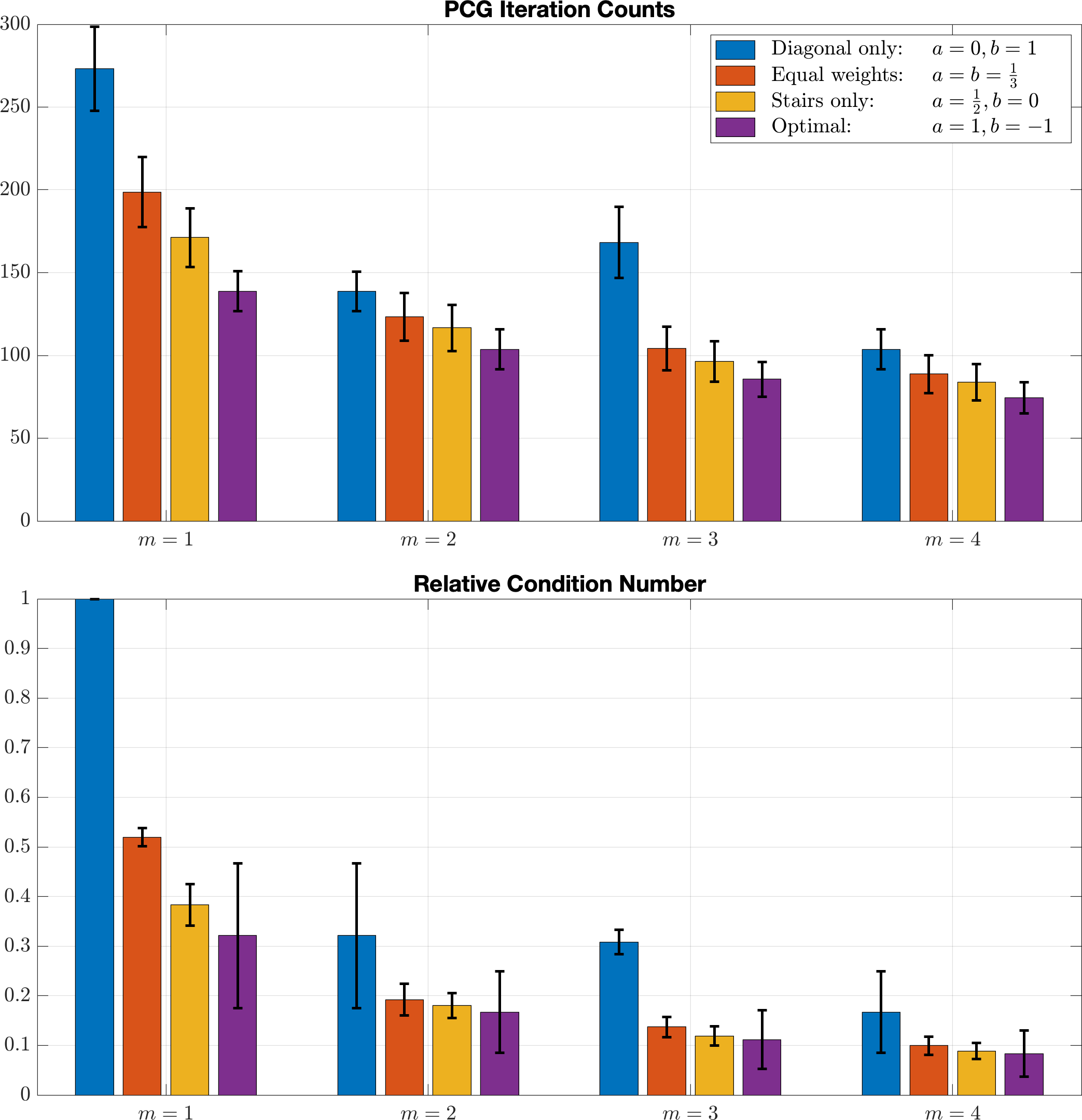
Figure 1: Average PCG iterations and condition number when varying $a,b$ for randomly generated s.p.d. block tridiagonal matrices with $N=20,n=15$. The purple bars correspond to the optimal pair $a=1,b=-1$ which is best on both metrics for all $m$.

IV Numerical results

In this section, we present a numerical evaluation of the $m$-step polynomial preconditioner (13) based on the proposed family of multi-splittings (12). We evaluate the resulting number of iterations of PCG needed for convergence (exiting condition: $\left\lVert Ax-b\right\rVert<1\mathrm{e}{-6}$) as well as relative condition number after preconditioning. We construct random s.p.d. block tridiagonal matrices and right hand side vectors by viewing the classical LQR problem as a Quadratic Program (QP), formulating the equivalent KKT system, and computing the Schur complement with respect to the Hessian as done in current state-of-the-art parallel solvers [7]. The resulting randomized, but structured, linear systems are then solved using our $m$-step preconditioners.

Figure 1 shows the average PCG iteration counts and relative condition number for varing polynomial orders $m$ and parameters $a,b$ in (13). “Diagonal only” corresponds to (15) where the diagonal splitting contributes to the multi-splitting only, “Stairs only” corresponds to (17) where only the stair splittings contribute, “Optimal” corresponds to (22) which is the optimal parametrization within (19), and “Equal weights” corresponds to equal weighting of the diagonal and stair splittings. For each setting, $50$ matrices $A$ and $100$ vectors $b$ are randomly generated for the PCG algorithm to solve $Ax=b$. The condition number are normalized to the “Diagonal only” + “$m=1$” case to enable comparison across settings which have large differences in the absolute condition number.

For all pairs of $a,b$, larger $m$ leads to smaller PCG iteration counts and condition number, as predicted in Remark 3.1. With $m=2,3,4$, the optimal $a=1,b=-1$ (purple) reduces on average $50\%,65\%,53\%$ of condition number and $25\%,49\%,28\%$ of PCG iteration counts compared with respective polynomial block Jacobi (blue) and $50\%,68\%,76\%$ of condition number and $25\%,38\%,46\%$ of PCG iteration counts compared with the its own base case $m=1$, which is the current state-of-the-art proposed by [19].

V Conclusion

In this study, we develop a family of $m$-step polynomial preconditioners tailored for symmetric positive definite block tridiagonal matrices. Building on the findings of [19], we extend the base case ($m=1$) to a general case of $m\in\mathbb{N}$, while preserving parallel efficiency. We also introduce the necessary and sufficient conditions, as well as a detailed analysis of the resulting eigenvalue distribution, for both both positive and negative parametrized multi-splittings, which form the basis of our family of preconditioners. We further demonstrate the uniqueness of the optimal parameters for the family root in terms of achieving a clustered spectrum, minimizing conjugate gradient (CG) iteration counts, and optimizing storage requirements. Numerical experiments substantiate all these theoretical claims showing as much as $76\%$ reduction in condition number and $46\%$ reduction in resulting PCG iterations for OCPs.

In future work, we aim to develop extensions to our approaches that further reduce the PCG iteration number, by parametrizing the polynomial (13) with proper coefficients [26]. We also aim to leverage the proposed preconditioner to improve upon existing parallel (S)QP solvers to solve OCPs more efficiently. Finally, we plan to apply our preconditioner to other scientific domains (e.g. solving PDE) where symmetric positive definite block tridiagonal matrices are prevalent.

-A Proof of Lemma 3.5

TABLE IV: Extreme points of $f_{a-}(\lambda)$ for $\lambda\in(0,1)$ if $a\in[0,1]$

$a$	max			min
	arg	reachable?	value	arg	reachable?	value
$[0,\frac{1}{3}]$	$0$	✗	$0$	$1$	✗	$2a-1\in[-1,-\frac{1}{3})$
$(\frac{1}{3},\frac{1}{2}]$	$0$	✗	$0$	$\lambda^{*}$	✓	$-\frac{(1-a)^{2}}{4a}\in(-\frac{1}{3},-\frac{1}{8}]$
$(\frac{1}{2},1]$	$1$	✗	$2a-1\in(0,1]$	$\lambda^{*}$	✓	$-\frac{(1-a)^{2}}{4a}\in(-\frac{1}{8},0]$

TABLE V: Range of $f_{a-}$, $1-f_{a-}$, and spectrum of $H_{ab},G_{ab}A$ if $a\in[0,1]$

$a$	range of $f_{a-}$	$\mathcal{I}_{H_{ab}}$	range of $1-f_{a-}$	$\mathcal{I}_{G_{ab}A}$
$[0,\frac{1}{3}]$	$(2a-1,0)$	$(2a-1,1)$	$(1,2-2a)$	$(0,2-2a)$
$(\frac{1}{3},\frac{1}{2}]$	$[-\frac{(1-a)^{2}}{4a},0)$	$[-\frac{(1-a)^{2}}{4a},1)$	$(1,1+\frac{(1-a)^{2}}{4a}]$	$(0,1+\frac{(1-a)^{2}}{4a}]$
$(\frac{1}{2},1]$	$[-\frac{(1-a)^{2}}{4a},2a-1)$	$[-\frac{(1-a)^{2}}{4a},1)$	$(2-2a,1+\frac{(1-a)^{2}}{4a}]$	$(0,1+\frac{(1-a)^{2}}{4a}]$

Proof.

All points are discussed in the most conservative scenario: $\lambda\in\sigma(B_{l}^{-1}C_{l})$ may take any value within $(0,1)$.

1. If $a\in[0,1]$:

   • $f_{a+}$ is monotonically increasing because $a$ and $1-a$ are non-negative. Since $f_{a+}(0)=0,f_{a+}(1)=1$, $f_{a+}\in(0,1)$ and $1-f_{a+}\in(0,1)$.

   • $f_{a-}$ is discussed case by case. The extreme points are summarized in Table IV.

     • If $a=0$, $f_{a-}=-\sqrt{\lambda}\in(-1,0)$ so it is monotonically decreasing.

     • If $a\in(0,1]$, calculate when the derivative vanishes: $f_{a-}(\lambda^{*})^{\prime}=0\Rightarrow\lambda^{*}=\frac{(1-a)^{2}}{4a^{2}}\geq 0$. Three candidate points for extreme: $f_{a-}(0)=0$, $f_{a-}(1)=2a-1$ and $f_{a-}(\lambda^{*})=-\frac{(1-a)^{2}}{4a}$.

     • If $\lambda^{*}\in(0,1)\Rightarrow\frac{(1-a)^{2}}{4a^{2}}<1\Rightarrow a>\frac{1}{3}$, $f_{a-}$ decreases on $(0,\lambda^{*})$ and increases on $(\lambda^{*},1)$. So $f_{a-}$ achieves its maximum at $\lambda=0$ or $\lambda=1$ (depends on whether $a\geq\frac{1}{2}$) and minimum at $\lambda^{*}$.

     • If $a\leq\frac{1}{3}\Rightarrow\lambda^{*}\geq 1$, $f_{a-}$ decreases on $(0,1)$, so the maximum is at $\lambda=0$ and minimum at $\lambda=1$.

   • $\rho(H_{ab})<1\Leftrightarrow\mathcal{I}_{H_{ab}}\subset(-1,1)$ is concluded from the third column of Table V. $\mathcal{I}_{G_{ab}A}\subset\mathbb{R}_{>0}$ and $\mu_{max}$ are concluded from the fifth column.

2. If $a\in(1,+\infty)$, $f_{a-}(\lambda)=a\lambda+(a-1)\sqrt{\lambda}$ is monotonically increasing because $a$ and $a-1$ are positive. $\frac{1}{a}\in(0,1)$ holds. $f_{a-}(\frac{1}{a})=1+(a-1)\sqrt{\frac{1}{a}}>1$, so $\forall\lambda\in[\frac{1}{a},1)$ leads to $\rho(H_{ab})>1$ and negative eigenvalues of $G_{ab}A$.

3. If $a\in(-\infty,0)$, $f_{a-}(\lambda)=a\lambda+(a-1)\sqrt{\lambda}<0$ is monotonically decreasing because $a$ and $a-1$ are negative. $\frac{1}{(1-a)^{2}}\in(0,1)$ holds. $f_{a-}(\frac{1}{(1-a)^{2}})=\frac{a}{(1-a)^{2}}-1<-1$, so $\forall\lambda\in[\frac{1}{(1-a)^{2}},1)$ leads to $\rho(H_{ab})>1$.
   $f_{a-}(\lambda)<0\Rightarrow 1-f_{a-}(\lambda)>0$, so the signs of eigenvalues of $G_{ab}A$ depend on $f_{a+}$:

   • The derivative of $f_{a+}$ vanishes at $\lambda^{*}=\frac{(1-a)^{2}}{4a^{2}}>0$.

   • If $\lambda^{*}\in(0,1)\Rightarrow\frac{(1-a)^{2}}{4a^{2}}<1\Rightarrow a<-1$, $f_{a+}$ increases on $(0,\lambda^{*})$, decreases on $(\lambda^{*},1)$, and achieves its maximum at $f_{a+}(\lambda^{*})=-\frac{(1-a)^{2}}{4a}>1\Rightarrow$ $G_{ab}A$ has negative eigenvalue.

   • If $a\geq-1\Rightarrow\lambda^{*}\geq 1$, $f_{a+}$ is monotonically increasing on $(0,1)$. So $f_{a+}(\lambda)\in(0,1)$ and $1-f_{a+}(\lambda)\in(0,1)$. At the same time, $f_{a-}\in(2a-1,0)$ and $1-f_{a-}\in(1,2-2a)$ coincide with the first rows of Tables IV and V.

All points are proved. ∎

References

- [1] J. T. Betts, “Survey of numerical methods for trajectory optimization,” Journal of guidance, control, and dynamics, vol. 21, no. 2, pp. 193–207, 1998.
- [2] F. R. Hogan, E. R. Grau, and A. Rodriguez, “Reactive planar manipulation with convex hybrid mpc,” in 2018 IEEE International Conference on Robotics and Automation (ICRA). IEEE, 2018, pp. 247–253.
- [3] J.-P. Sleiman, F. Farshidian, M. V. Minniti, and M. Hutter, “A unified mpc framework for whole-body dynamic locomotion and manipulation,” IEEE Robotics and Automation Letters, vol. 6, no. 3, pp. 4688–4695, 2021.
- [4] R. Grandia, F. Jenelten, S. Yang, F. Farshidian, and M. Hutter, “Perceptive locomotion through nonlinear model-predictive control,” IEEE Transactions on Robotics, vol. 39, no. 5, pp. 3402–3421, 2023.
- [5] M. Tranzatto, F. Mascarich, L. Bernreiter, C. Godinho, M. Camurri, S. Khattak, T. Dang, V. Reijgwart, J. Loeje, D. Wisth et al., “Cerberus: Autonomous legged and aerial robotic exploration in the tunnel and urban circuits of the darpa subterranean challenge,” arXiv preprint arXiv:2201.07067, vol. 3, 2022.
- [6] P. M. Wensing, M. Posa, Y. Hu, A. Escande, N. Mansard, and A. Del Prete, “Optimization-based control for dynamic legged robots,” IEEE Transactions on Robotics, vol. 40, pp. 43–63, 2023.
- [7] E. Adabag, M. Atal, W. Gerard, and B. Plancher, “Mpcgpu: Real-time nonlinear model predictive control through preconditioned conjugate gradient on the gpu,” in 2024 IEEE International Conference on Robotics and Automation (ICRA). IEEE, 2024, pp. 9787–9794.
- [8] K. Nguyen, S. Schoedel, A. Alavilli, B. Plancher, and Z. Manchester, “Tinympc: Model-predictive control on resource-constrained microcontrollers,” in 2024 IEEE International Conference on Robotics and Automation (ICRA). IEEE, 2024, pp. 1–7.
- [9] H. Esmaeilzadeh, E. Blem, R. St. Amant, K. Sankaralingam, and D. Burger, “Dark silicon and the end of multicore scaling,” in Proceedings of the 38th annual international symposium on Computer architecture, 2011, pp. 365–376.
- [10] G. Venkatesh, J. Sampson, N. Goulding, S. Garcia, V. Bryksin, J. Lugo-Martinez, S. Swanson, and M. B. Taylor, “Conservation cores: reducing the energy of mature computations,” ACM Sigplan Notices, vol. 45, no. 3, pp. 205–218, 2010.
- [11] S. C. Eisenstat, “Efficient implementation of a class of preconditioned conjugate gradient methods,” SIAM Journal on Scientific and Statistical Computing, vol. 2, no. 1, pp. 1–4, 1981.
- [12] R. Helfenstein and J. Koko, “Parallel preconditioned conjugate gradient algorithm on gpu,” Journal of Computational and Applied Mathematics, vol. 236, no. 15, pp. 3584–3590, 2012.
- [13] M. Schubiger, G. Banjac, and J. Lygeros, “Gpu acceleration of admm for large-scale quadratic programming,” Journal of Parallel and Distributed Computing, vol. 144, pp. 55–67, 2020.
- [14] Y. Saad, Iterative methods for sparse linear systems. SIAM, 2003.
- [15] J. H. Yun, “Block incomplete factorization preconditioners for a symmetric block-tridiagonal m-matrix,” Journal of computational and applied mathematics, vol. 94, no. 2, pp. 133–152, 1998.
- [16] P. Concus, G. H. Golub, and G. Meurant, “Block preconditioning for the conjugate gradient method,” SIAM Journal on Scientific and Statistical Computing, vol. 6, no. 1, pp. 220–252, 1985.
- [17] F. Di Benedetto, G. Fiorentino, and S. Serra, “Cg preconditioning for toeplitz matrices,” Computers & Mathematics with Applications, vol. 25, no. 6, pp. 35–45, 1993.
- [18] Z. Qu, W. Gao, O. Hinder, Y. Ye, and Z. Zhou, “Optimal diagonal preconditioning,” Operations Research, 2024.
- [19] X. Bu and B. Plancher, “Symmetric stair preconditioning of linear systems for parallel trajectory optimization,” in 2024 IEEE International Conference on Robotics and Automation (ICRA). IEEE, 2024, pp. 9779–9786.
- [20] J. M. Ortega, Numerical analysis: a second course. SIAM, 1990.
- [21] D. P. O’leary and R. E. White, “Multi-splittings of matrices and parallel solution of linear systems,” SIAM Journal on algebraic discrete methods, vol. 6, no. 4, pp. 630–640, 1985.
- [22] C. Neumann, Untersuchungen über das logarithmische und Newton’sche Potential. BG Teubner, 1877.
- [23] L. Adams, “M-step preconditioned conjugate gradient methods,” SIAM Journal on Scientific and Statistical Computing, vol. 6, no. 2, pp. 452–463, 1985.
- [24] H. Lu, “Stair matrices and their generalizations with applications to iterative methods i: A generalization of the successive overrelaxation method,” SIAM journal on numerical analysis, vol. 37, no. 1, pp. 1–17, 1999.
- [25] J. Nocedal and S. J. Wright, Numerical optimization. Springer, 1999.
- [26] Y. Saad, “Practical use of polynomial preconditionings for the conjugate gradient method,” SIAM Journal on Scientific and Statistical Computing, vol. 6, no. 4, pp. 865–881, 1985.