Satellite Selection for In-Band
Coexistence of Dense LEO Networks

Abstract

We study spectrum sharing between two dense low-earth orbit (LEO) satellite constellations, an incumbent primary system and a secondary system that must respect interference protection constraints on the primary system. In particular, we propose a secondary satellite selection framework and algorithm that maximizes capacity while guaranteeing that the time-average interference and absolute interference inflicted upon each primary ground user never exceeds specified thresholds. We solve this NP-hard constrained, combinatorial satellite selection problem through Lagrangian relaxation to decompose it into simpler problems which can then be solved through subgradient methods. A high-fidelity simulation is developed based on public FCC filings and technical specifications of the Starlink and Kuiper systems. We use this case study to illustrate the effectiveness of our approach and that explicit protection is indeed necessary for healthy coexistence. We further demonstrate that deep learning models can be used to predict the primary satellite system associations, which helps the secondary system avoid inflicting excessive interference and maximize its own capacity.

I Introduction

Dense low-earth orbit (LEO) satellite constellations are poised to play a vital role in delivering seamless global broadband wireless services across the globe [1, 2, 3, 4]. With Starlink, a prominent frontrunner, already delivering commercial services using more than 6,000 satellites in orbit [5], the potential of LEO networks to bridge connectivity gaps and provide universal broadband access is increasingly evident. In addition to Starlink, other companies like OneWeb, AST Spacemobile, Amazon, and other emerging players are actively advancing LEO satellite communication systems for a variety of use cases including direct-to-handset.

To facilitate fair and efficient spectrum sharing, the Federal Communications Commission (FCC) gives precedence (or incumbency) to LEO systems which applied for launch rights in earlier so-called processing rounds, referred to as primary systems, than others [6], termed secondary systems. Consequently, it is the expectation of the FCC that each system either coordinates with or protects systems which acquired launch rights in earlier processing rounds [6]. This work examines how two dense LEO satellite systems—one the primary and the other secondary—can coexist in the same frequency band under such expectations. Specifically, we investigate practical mechanisms for the secondary system to determine its satellite-to-ground cell associations, choosing which satellite should serve each ground cell. The goal is to optimize the secondary system’s performance while ensuring it does not inflict excessive interference onto ground users of the primary system.

I-A Background and Related Work

The principle of spectrum sharing is concerned with so-called secondary systems not inflicting significant interference onto primary (or incumbent) systems when attempting to operate in some portion of frequency spectrum [7, 8, 9]. Extensive research has explored various cognitive radio (CR) techniques to enable such spectrum sharing, but the practical deployment of these conventional CR paradigms remains limited. Spectrum sharing in LEO satellite communications introduces additional complexities due to the high mobility of satellites and substantial communication link latency [10], leading to outdated spectrum perception and diminished effectiveness of traditional spectrum access strategies [11]. Despite the shortcomings of CR techniques, LEO satellite communications offer a unique opportunity for revitalizing spectrum sharing strategies. Several key factors contribute to this potential: (i) highly directional communication links, which result in some natural orthogonality, (ii) known satellite locations in space, which usually have predictable line-of-sight propagation to Earth, (iii) advances in machine learning (ML) for spectrum prediction and resource optimization, and (iv) the absence of alternative spectrum-sharing solutions suitable for the LEO environment.

ML-driven spectrum inference utilizes historical and real-time data to predict spectrum occupancy and environmental dynamics, enabling a transition from reactive sensing to proactive prediction and enhancing spectrum management and decision-making [12]. ML-powered CR systems integrate two key capabilities: perception, which predicts spectrum occupancy and primary system behavior, and reconfigurability, which optimizes spectrum access and resource allocation [13]. Most environment perception schemes in CR systems, including satellite communication systems, primarily focus on predicting spectrum occupancy—that is, determining whether the primary system is actively using the spectrum—using various neural network architectures [14, 15, 16, 17]. Understanding spectrum usage of the primary system is vital, but in satellite systems, it is especially critical to identify directions in which primary satellites and ground users steer their beams. This directional information and separation allows secondary systems to share frequency resources even when the primary system is active [18]. Existing studies emphasize that avoiding interference in specific angular directions—referred to as “avoidance angles” can effectively safeguard geostationary satellite systems from harmful interference from non-geostationary orbit (NGSO) systems [19]. Additionally, this approach has demonstrated potential in mitigating interference between NGSO satellites, including those in LEO and medium-earth orbit [20, 18, 21, 22].

Building on spectrum prediction, reinforcement learning is often proposed for dynamic spectrum access decisions [23, 24] in relatively small and simple satellite systems. However, the application of reinforcement learning to larger and more complex systems is extremely difficult due to the increased state and action spaces, resulting in slower convergence and higher computational overhead [25, 26]. In dense LEO networks, the challenge extends beyond simple spectrum access decisions. Rather, it involves determining the optimal satellite-to-ground cell associations across an entire constellation of multi-beam satellites to maximize the secondary system’s spectrum utilization while guaranteeing sufficient protection of primary users—which is the focus of this work.

I-B Contributions

Our recent work [22] demonstrated that in-band coexistence of two dense LEO satellite systems is in principle feasible through strategic satellite selection, meaning that the secondary system would have at least one satellite that could serve a given secondary ground user in light of the primary satellite-to-ground user association. In other words, no matter what the primary system is doing as far as serving its ground users, the secondary system can in principle work around it, since it has at least one satellite that can avoid interfering with any hypothetical primary ground user. While this is an encouraging result, how to actually execute such a selection reliably and on global scale was left as an open problem. We are unaware of any other work that solves such a problem.

The main contribution of the present paper, therefore, is to propose a framework and practical algorithm for optimal satellite selection across a secondary constellation. Optimal in this context being defined as maximizing the capacity of the secondary system while limiting the interference it inflicts onto primary users, meanwhile accounting for any other operational constraints. The interference protection constraint has often been formulated in quite a strict manner, limiting the increase in the effective temperature of a primary user’s receiver to be no more than 6% [27, 28] due to interference from the secondary system, which translates to an interference-to-noise ratio (INR) of at most $-12.2$ dB.

Novel framework and formulation for LEO spectrum sharing. Our work formulates a novel interference protection constraint and shows that it offers more flexibility to the secondary system in its satellite selection, while still offering comparable levels of protection as the aforementioned strict $-12.2$ dB constraint. We then employ this proposed constraint to formulate a satellite selection problem which aims to maximize the capacity of the secondary system while limiting the interference inflicted upon each primary ground user—both in an absolute sense and time-averaged sense. This problem formulation and our approach to solving it are centered on grouping ground cells into clusters, each of which is served by a single satellite. This not only offers dimensionality reduction and mathematical tractability but also aligns well with the operation of practical deployments like Starlink and Kuiper.

Practical algorithm to achieve optimal satellite associations. We develop a practical algorithm by transforming the challenging combinatorial nature of the formulated NP-hard problem into a sequence of simpler problems via Langrangian relaxation, each of which can be solved through subgradient iterations. In turn, our satellite selection mechanism offers computational efficiency yet remains capable of reliably protecting primary ground users from excessive interference. Conceptually, this is accomplished through strategically associating secondary cells with satellites which are spatially separated from active primary satellites serving nearby ground cells—offering protection to primary ground users while also reducing the interference received by secondary ground users from primary satellites.

High-fidelity simulation of Starlink and Kuiper inter-operation. We develop a high-fidelity simulation of two prominent LEO satellite systems—Starlink as the primary system and Kuiper as the secondary system—each consisting of thousands of satellites, using publicly available data from their FCC filings [29, 30]. To ensure regulatory compliance, we implement a power control mechanism that adjusts transmission power based on the satellite’s path distance while adhering to maximum effective isotropic radiated power (EIRP) and power flux density (PFD) limits [31]. The simulation models each system’s satellite-to-cluster associations as satellites traverse their orbits, incorporating satellite handover dynamics across multiple ground cells and association policies. Ground cells are modeled using Earth-centered Earth-fixed (ECEF) coordinates [10], and each satellite is equipped with multiple spot beams [30, 32, 33], following a predefined transmit beam gain pattern within the beam mask [34]. Each beam is allocated to a single ground cell at any given time [30], utilizing a specific time and frequency resource.

While there is an inherent trade-off between the secondary system’s capacity and the level of protection afforded to the primary system, results indicate that the secondary system can coexist with the primary system using the proposed secondary satellite selection algorithm. Our proposed interference protection constraint introduces flexibility in secondary satellite selection while maintaining a well-controlled compromise in protection. Furthermore, we demonstrate that secondary satellite selection can be effectively performed by leveraging deep learning (DL) models that learn an undisclosed underlying primary satellite association policy. These learned models can then be employed to optimize the proposed secondary satellite selection process.

II System Model

In this section, we present the system model and key performance metrics necessary for analyzing the coexistence of two dense LEO satellite systems. We begin by defining the satellite systems’ ground cell planning methodology over a wide geographical area. We then define the set of available satellites capable of serving these ground cells and establish performance metrics based on satellite-to-ground associations. This provides a structured framework for evaluating spectrum sharing and inter-system interference management in the coexistence scenario considered in this work.

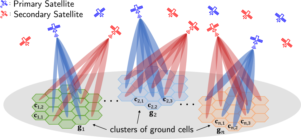
Figure 1: Primary and secondary satellite systems serve their ground users with multiple satellites, each forming $N_{\mathrm{B}}$ spot beams. Cluster ${{\mathbf{g}}}_{n}$ is served by a single satellite and consists of ${N_{\mathrm{C}}}\gg N_{\mathrm{B}}$ ground cells ${{\mathbf{c}}}_{n,\ell}$, with each cell served by a single spot beam.

II-A Ground Cells and Clusters

Satellites serve ground users by forming $N_{\mathrm{B}}$ highly directional spot beams per satellite at once. The area served by each spot beam is termed a cell—typically spanning $300$–$500$ km² [30]—and the cells formed by a single satellite are tessellated on the ground, often in a hexagonal arrangement similar to those in terrestrial networks. With its multiple spot beams, each satellite is assumed responsible for serving a cluster of ${N_{\mathrm{C}}}$ cells during the time period between handovers. In practical systems, it is often the case that $N_{\mathrm{B}}\ll{N_{\mathrm{C}}}$, with $N_{\mathrm{B}}$ on the order of $16$ [32, 33], and thus each satellite must employ spatial, time, and/or frequency multiplexing [35, 30] to provide adequate coverage over a wide area. Each cluster of ${N_{\mathrm{C}}}$ cells is fixed over time, though the satellite serving them will certainly change. For simplicity of notation, let us assume the primary and secondary systems aim to serve their respective ground users distributed across overlapping cells and clusters, as illustrated in Figure 1. With this, let $\mathcal{G}$ be the set of ${N_{\mathrm{G}}}$ clusters spanning some region of interest, defined as

$$\mathcal{G}={\left\{{{\mathbf{g}}}_{n}:n={1,\dots,{N_{\mathrm{G}}}}\right\}},$$ (1)

where ${{\mathbf{g}}}_{n}$ denotes the $n$-th cluster of ${N_{\mathrm{C}}}$ ground cells ${{\mathbf{g}}}_{n}={\left\{{{\mathbf{c}}}_{n,\ell}:\ell=1,\dots,N_{\mathrm{C}}\right\}}$. To provide some context, the geographical area of interest used in our numerical results is shown in Figure 2, where each hexagon represents a cluster consisting of ${N_{\mathrm{C}}}=127$ cells. This clustering coincides with coverage provided by practical multi-beam LEO satellites like Starlink [35, 36].

II-B Available Satellites and Ground Associations

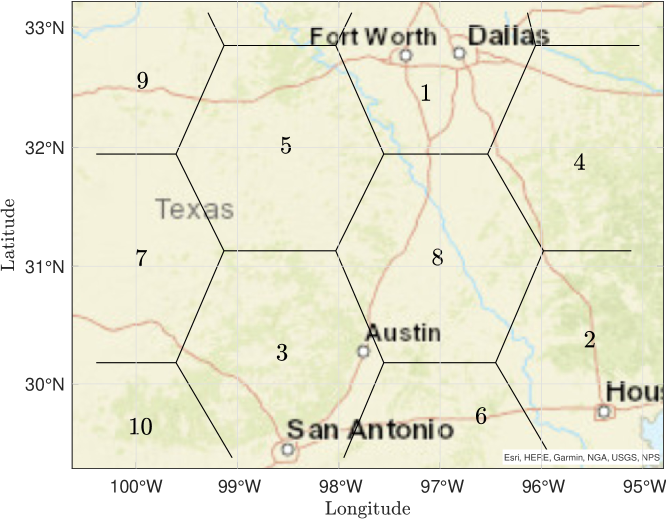
Figure 2: Geographical region considered in this work. Each hexagon represents a cluster with ${N_{\mathrm{C}}}=127$ cells.

Let $\bar{\mathcal{P}}^{t}={\left\{{{\mathbf{p}}}^{t}_{i}:i=1,\dots,{N_{\mathrm{P}}}\right\}}$ denote the set of all ${N_{\mathrm{P}}}$ satellites in the primary constellation at time $t$, with ${{\mathbf{p}}}_{i}^{t}$ denoting the $i$-th primary satellite at time $t$. Similarly, let $\bar{\mathcal{S}}^{t}={\left\{{{\mathbf{s}}}^{t}_{m}:m=1,\dots,{N_{\mathrm{S}}}\right\}}$ be the set of all ${N_{\mathrm{S}}}$ satellites in the secondary system’s constellation at time $t$, with ${{\mathbf{s}}}_{m}^{t}$ being the $m$-th secondary satellite at time $t$. Out of all satellites in orbit, only those whose elevation angle—relative to a specified ground location—which exceeds the minimum elevation angle $\epsilon_{\mathrm{min}}$ can transmit signals toward that ground location, according to regulations [36, 30]. Thus, the overhead sets of primary and secondary satellites capable of serving a particular ground cluster ${{\mathbf{g}}}_{n}$ at time $t$ can be defined as

$$\mathcal{P}^{t}_{n}={\left\{{{\mathbf{p}}}\in\overline{\mathcal{P}}^{t}:\epsilon({{\mathbf{g}}}_{n},{{\mathbf{p}}})\geq\epsilon_{\mathrm{min}}\right\}},$$ (2)

$$\mathcal{S}^{t}_{n}={\left\{{{\mathbf{s}}}\in\overline{\mathcal{S}}^{t}:\epsilon({{\mathbf{g}}}_{n},{{\mathbf{s}}})\geq\epsilon_{\mathrm{min}}\right\}},$$ (3)

where $\epsilon({{\mathbf{g}}}_{n},{{\mathbf{x}}})$ denotes the minimum elevation of a satellite ${{\mathbf{x}}}$ relative to the horizon at any location within ground cluster ${{\mathbf{g}}}_{n}$. Building on this definition of overhead satellites, which is established with respect to a single cluster ${{\mathbf{g}}}_{n}$, we define the set of all satellites spanning clusters in $\mathcal{G}$ at time $t$ as

$$\mathcal{P}^{t}_{\mathcal{G}}=\mathcal{P}^{t}_{1}\cup\cdots\cup\mathcal{P}^{t}_{{N_{\mathrm{G}}}},$$ (4)

$$\mathcal{S}^{t}_{\mathcal{G}}=\mathcal{S}^{t}_{1}\cup\cdots\cup\mathcal{S}^{t}_{{N_{\mathrm{G}}}}.$$ (5)

We are particularly interested in how the secondary system satellites are associated to serve each cluster. Let us therefore define $x^{t}_{m,n}$ as a binary satellite-to-cluster association variable

$$x^{t}_{m,n}=\begin{cases}1,&\parbox[t]{156.49014pt}{if the $m$-th secondary satellite serves cells in cluster ${{\mathbf{g}}}_{n}$ at time $t$}\\ 0,&\text{otherwise}.\end{cases}$$ (6)

Let us denote by ${\mathbf{X}}^{t}\in{\left\{0,1\right\}}^{{N_{\mathrm{S}}}\times{N_{\mathrm{G}}}}$ the secondary system association matrix at time $t$ containing all binary association variables $x_{m,n}^{t}$. Considering each satellite has a limited capacity and limited number of spot beams [32, 33], we assume that clusters are sized such that each satellite may only serve one cluster at any given time $t$, leading to the constraint

$$\sum_{n=1}^{{N_{\mathrm{G}}}}x^{t}_{m,n}\leq 1\ \forall\ m=1,2,\dots,{N_{\mathrm{S}}},$$ (7)

It is also reasonable to assume that, at a given frequency, a single cluster may only be served by one satellite at any given time to avoid intra-system interference, meaning

$$\sum_{m=1}^{{N_{\mathrm{S}}}}x^{t}_{m,n}\leq 1\ \forall\ n=1,2,\dots,{N_{\mathrm{G}}}.$$ (8)

Having assumed a single satellite may not necessarily serve all cells in a cluster at a given time due to a limited number of spot beams, we also define the binary satellite-to-cell association variable of the secondary system at time $t$ within a cluster as

$$y^{t}_{m,n,\ell}=\begin{cases}1,&\parbox[t]{156.49014pt}{if the $m$-th secondary satellite serves the $\ell$-th cell ${{\mathbf{c}}}_{n,\ell}$ in cluster $n$ at time $t$}\\ 0,&\text{otherwise}.\end{cases}$$ (9)

The number of cells served by a satellite at once within a single cluster is bounded by its number of spot beams, i.e.,

$$\sum_{\ell=1}^{{N_{\mathrm{C}}}}y^{t}_{m,n,\ell}\leq N_{\mathrm{B}}\ \forall\ m,n,t.\vskip-8.5359pt$$ (10)

II-C Key Performance Metrics

Let us define the transmit antenna gain of primary satellite ${{\mathbf{p}}}$ in the direction of a primary user ${\mathtt{u}}$ as ${G_{\mathrm{tx}}}({\mathtt{u}},{{\mathbf{p}}},{{\mathbf{c}}})$ when ${{\mathbf{p}}}$ steers its beam toward ${{\mathbf{c}}}$. Similarly, let ${G_{\mathrm{rx}}}({\mathtt{u}},{{\mathbf{p}}})$ denote the receive antenna gain of the primary user ${\mathtt{u}}$ in the direction of the primary satellite ${{\mathbf{p}}}$. Path loss between a user ${\mathtt{u}}$ and satellite ${{\mathbf{p}}}$ is denoted by $L({\mathtt{u}},{{\mathbf{p}}})$ and modeled as [10]

$${\left[L({\mathtt{u}},{{\mathbf{p}}})\right]}_{\mathrm{dB}}=32.45+20\,\mathrm{log}_{10}{\left(f\right)}+20\,\mathrm{log}_{10}{\left(d({\mathtt{u}},{{\mathbf{p}}})\right)},$$ (11)

where $f$ is the carrier frequency and $d({\mathtt{u}},{{\mathbf{p}}})$ is the path distance between ${\mathtt{u}}$ and ${{\mathbf{p}}}$. Based on these definitions, the signal-to-noise ratio (SNR) at a primary ground user ${\mathtt{u}}$ in cell ${{\mathbf{c}}}$ when receiving from its serving satellite ${{\mathbf{p}}}$ is given by

$$\mathsf{SNR}({\mathtt{u}},{{\mathbf{p}}},{{\mathbf{c}}})=\frac{{P_{\mathrm{tx}}}({{\mathbf{p}}})\ {G_{\mathrm{tx}}}({\mathtt{u}},{{\mathbf{p}}},{{\mathbf{c}}})\ {G_{\mathrm{rx}}}({\mathtt{u}},{{\mathbf{p}}})}{{P_{\mathrm{n}}}({\mathtt{u}})\ L({\mathtt{u}},{{\mathbf{p}}})},$$ (12)

where ${P_{\mathrm{tx}}}({{\mathbf{p}}})$ represents the transmit power of satellite ${{\mathbf{p}}}$, and ${P_{\mathrm{n}}}({\mathtt{u}})$ denotes the noise power at user ${\mathtt{u}}$.

In this work, we are interested in the downlink interference inflicted onto a primary user ${\mathtt{u}}$ by secondary satellites. Let us thus suppose a secondary satellite ${{\mathbf{s}}}$ steers its beam toward cell ${{\mathbf{c}}}$ and, in doing so, inflicts interference onto primary ground user ${\mathtt{u}}$ being served by a satellite ${{\mathbf{p}}}$. Then, the resulting INR at the primary ground user ${\mathtt{u}}$ can be written as

$$\mathsf{INR}({\mathtt{u}},{{\mathbf{p}}};{{\mathbf{s}}},{{\mathbf{c}}})=\frac{{P_{\mathrm{tx}}}({{\mathbf{s}}})\ {G_{\mathrm{tx}}}({\mathtt{u}};{{\mathbf{s}}},{{\mathbf{c}}})\ {G_{\mathrm{rx}}}({\mathtt{u}},{{\mathbf{p}}};{{\mathbf{s}}},{{\mathbf{c}}})}{{P_{\mathrm{n}}}({\mathtt{u}})\ L({\mathtt{u}},{{\mathbf{s}}})}.$$ (13)

Here, we have slightly extended the notation of ${G_{\mathrm{tx}}}(\cdot)$ and ${G_{\mathrm{rx}}}(\cdot)$ to make it clear that ${G_{\mathrm{tx}}}({\mathtt{u}};{{\mathbf{s}}},{{\mathbf{c}}})$ represents the transmit gain of satellite ${{\mathbf{s}}}$ in the direction of the primary user ${\mathtt{u}}$ when ${{\mathbf{s}}}$ serves its ground cell ${{\mathbf{c}}}$. Similarly, ${G_{\mathrm{rx}}}({\mathtt{u}},{{\mathbf{p}}};{{\mathbf{s}}},{{\mathbf{c}}})$ represents the receive gain in the direction of the secondary satellite ${{\mathbf{s}}}$ when the user ${\mathtt{u}}$ steers its beam toward its serving satellite ${{\mathbf{p}}}$.

Having considered multiple satellites serving multiple ground cells, we are concerned with the aggregate interference inflicted onto a given primary user by all active spot beams in the secondary system. Let us define the collective interference inflicted by a single secondary satellite ${{\mathbf{s}}}_{m}$ onto a primary user ${\mathtt{u}}$ at time $t$ as

$$\mathsf{INR}^{t}({\mathtt{u}},{{\mathbf{p}}};{{\mathbf{s}}}^{t}_{m},{{\mathbf{g}}}_{n})\triangleq\sum_{\ell=1}^{{N_{\mathrm{C}}}}\mathsf{INR}^{t}({\mathtt{u}},{{\mathbf{p}}};{{\mathbf{s}}}^{t}_{m},{{\mathbf{c}}}_{n,\ell})\cdot y^{t}_{m,n,\ell},$$ (14)

where the user has steered its beam toward satellite ${{\mathbf{p}}}$.

Recall, the binary association variable $x^{t}_{m,n}$ indicates whether secondary satellite ${{\mathbf{s}}}_{m}$ actively serves cluster ${{\mathbf{g}}}_{n}$ at time $t$, thereby contributing interference to the primary user ${\mathtt{u}}$. The aggregate interference inflicted upon primary user ${\mathtt{u}}$ by all secondary satellites at time $t$ can thus be stated as

$$\mathsf{INR}^{t}({\mathtt{u}},{{\mathbf{p}}})\triangleq\sum_{m=1}^{{N_{\mathrm{S}}}}\sum_{n=1}^{N_{\mathrm{G}}}\mathsf{INR}^{t}({\mathtt{u}},{{\mathbf{p}}};{{\mathbf{s}}}^{t}_{m},{{\mathbf{g}}}_{n})\cdot x^{t}_{m,n}.$$ (15)

The signal-to-interference-plus-noise ratio (SINR) of a primary user ${\mathtt{u}}$ in cell ${{\mathbf{c}}}$ when served by satellite ${{\mathbf{p}}}$ at time $t$ is then

$$\mathsf{SINR}^{t}({\mathtt{u}},{{\mathbf{p}}},{{\mathbf{c}}})=\frac{\mathsf{SNR}^{t}({\mathtt{u}},{{\mathbf{p}}},{{\mathbf{c}}})}{1+\mathsf{INR}^{t}({\mathtt{u}},{{\mathbf{p}}})},$$ (16)

where intra-system interference inflicted by the primary system onto its own users has been ignored for simplicity. In a similar manner, the SINR of a secondary user ${\mathtt{v}}$ served by secondary satellite ${{\mathbf{s}}}$ at time $t$ is of the form

$$\mathsf{SINR}^{t}({\mathtt{v}},{{\mathbf{s}}},{{\mathbf{c}}})=\frac{\mathsf{SNR}^{t}({\mathtt{v}},{{\mathbf{s}}},{{\mathbf{c}}})}{1+\mathsf{INR}^{t}({\mathtt{v}},{{\mathbf{s}}})},$$ (17)

where $\mathsf{INR}^{t}({\mathtt{v}},{{\mathbf{s}}})$ is analogously the aggregate interference inflicted upon ${\mathtt{v}}$ by the primary system.

III Optimizing Secondary Satellite
Selection for Coexistence

In our prior work [22], we showed that there is promise in enabling the LEO coexistence paradigm laid forth through the strategic selection of secondary serving satellites—courtesy of the spatial diversity across primary and secondary satellite constellations at virtually any given time. Creating practical mechanisms to perform such a selection on a network scale remains an open problem, however, which amounts to optimizing the secondary system satellite-cluster association matrix ${\mathbf{X}}^{t}$ over time $t$ to maximize a desired objective while abiding by certain constraints. More specifically, in selecting which secondary satellites serve its ground users, we aim to maximize the downlink performance of the secondary satellite system while guaranteeing primary ground users are protected from a certain level of interference inflicted by secondary satellites.

III-A Interference Protection Constraint

$$\max_{{\mathtt{u}}\in\mathcal{U}}\,\underset{\tau\in[t-{T_{\mathrm{w}}},t+{T_{\mathrm{h}}})}{\mathbb{E}}{\left[\mathsf{INR}^{\tau}({\mathtt{u}},{{\mathbf{p}}}^{\tau}_{\mathtt{u}})\right]} \leq\frac{1}{T_{\mathrm{w}}+T_{\mathrm{h}}}{\left[\max_{{\mathtt{u}}\in\mathcal{U}}\,\sum_{\tau=t-T_{\mathrm{w}}}^{t-1}\mathsf{INR}^{\tau}({\mathtt{u}},{{\mathbf{p}}}^{\tau}_{\mathtt{u}})+\max_{{\mathtt{u}}\in\mathcal{U}}\,\sum_{\tau=t}^{t+T_{\mathrm{h}}-1}\mathsf{INR}^{\tau}({\mathtt{u}},{{\mathbf{p}}}^{\tau}_{\mathtt{u}})\right]}$$ (22)

$$\max_{{\mathtt{u}}\in\mathcal{U}}\,\frac{1}{{T_{\mathrm{h}}}}\sum_{\tau=t}^{t+T_{\mathrm{h}}-1}\mathsf{INR}^{\tau}({\mathtt{u}},{{\mathbf{p}}}^{\tau}_{\mathtt{u}})\leq\underbrace{\frac{1}{{T_{\mathrm{h}}}}{\left[{\left({T_{\mathrm{w}}}+{T_{\mathrm{h}}}\right)}\cdot\overline{\mathsf{INR}}_{\mathrm{th}}-\max_{{\mathtt{u}}\in\mathcal{U}}\sum_{\tau=t-T_{\mathrm{w}}}^{t-1}\mathsf{INR}^{\tau}({\mathtt{u}},{{\mathbf{p}}}^{\tau}_{\mathtt{u}})\right]}}_{\triangleq\,\overline{\mathsf{INR}}_{\mathrm{th}}^{t}}$$ (23)

$$\frac{1}{{T_{\mathrm{h}}}}\sum_{\tau=t}^{t+T_{\mathrm{h}}-1}\mathsf{INR}^{\tau}({\mathtt{u}},{{\mathbf{p}}}^{\tau}_{\mathtt{u}})=\sum_{m=1}^{{N_{\mathrm{S}}}}\sum_{n=1}^{N_{\mathrm{G}}}\underbrace{\frac{1}{{T_{\mathrm{h}}}}\sum_{\tau=t}^{t+T_{\mathrm{h}}-1}\mathsf{INR}^{\tau}({\mathtt{u}},{{\mathbf{p}}}^{\tau}_{\mathtt{u}};{{\mathbf{s}}}_{m},{{\mathbf{g}}}_{n})}_{\triangleq\,\overline{\mathsf{INR}}_{{T_{\mathrm{h}}}}^{t}({\mathtt{u}},{{\mathbf{p}}}_{\mathtt{u}};{{\mathbf{s}}}_{m},{{\mathbf{g}}}_{n})}\,x^{t}_{m,n}.$$ (24)

 

The key condition for the secondary system to coexist with the primary system is that it must not inflict prohibitive interference on the primary system. Defining an interference protection constraint is therefore important in the context of this work, especially since the precise definition of prohibitive interference remains fluid, especially on a global scale [27, 37]. Recall, the aggregate interference inflicted by the secondary system upon a given ground user ${\mathtt{u}}$ at time $t$ is denoted by $\mathsf{INR}^{t}({\mathtt{u}},{{\mathbf{p}}}_{\mathtt{u}})$ and is calculated by summing the interference inflicted by all active spot beams of satellites, as defined in (15). Perhaps the simplest yet strictest way to define an interference protection constraint is therefore to require that the aggregate interference be below a specified threshold $\mathsf{INR}_{\mathrm{th}}$ at all primary users and at all times, i.e.,

$$\mathsf{INR}^{t}({\mathtt{u}},{{\mathbf{p}}}^{t}_{\mathtt{u}})\leq\mathsf{INR}_{\mathrm{th}}\ \forall\ {\mathtt{u}}\in\mathcal{U},\ t\in[0,\infty),$$ (18)

where ${{\mathbf{p}}}^{t}_{\mathtt{u}}$ is the serving satellite of ${\mathtt{u}}$ at time $t$ and $\mathcal{U}$ is the set of all primary ground users to protect. While this strict constraint is intuitive and certainly very protective, we have found it to be too restrictive for realistic thresholds $\mathsf{INR}_{\mathrm{th}}$, often leading to poor utilization of the secondary system, as we will show in numerical results. Furthermore, when employing this strict constraint, we found that interference levels fall well below $\mathsf{INR}_{\mathrm{th}}$ for most users the majority of the time. This motivates us to consider more flexible still well-defined interference protection constraints.

In this pursuit, we formalize three proposed principles. First, since handover in practical LEO systems usually happens on time scales of seconds or tens of seconds [38, 39], protection should be proactive in the sense that it should be guaranteed throughout the time period between handovers. Second, given the complexity and time-varying nature of this coexistence paradigm, infrequent, short-lived spikes in interference at a given user are extremely difficult to completely eliminate without frequent service interruptions and should thus be forgiven to a certain extent, to facilitate plausible coexistence. Third, interference should nonetheless never exceed a specified threshold at any given primary user.

To properly formulate a constraint with these principles in mind, suppose we are interested in performing secondary satellite-cluster association at time $t$, i.e., we seek to optimize ${\mathbf{X}}^{t}$. Let us denote by $T_{\mathrm{h}}>0$ the time between secondary system handovers, and assume that secondary association is fixed between handover instances, after which a new association will be made. Put simply, if a handover is performed at time $t$, then ${\mathbf{X}}^{t}={\mathbf{X}}^{\tau}\ \forall\ \tau\in[t,t+T_{\mathrm{h}})$. It is important to keep in mind, however, that interference levels will nonetheless fluctuate throughout the handover period $[t,t+T_{\mathrm{h}})$, since both the secondary and primary satellites will move along their orbits. Now, if interference had been relatively high leading up to handover time $t$, it is sensible to be less tolerable of interference during the upcoming handover period $[t,t+T_{\mathrm{h}})$, and vice versa. To capture this, let us formulate the following constraint on the time-averaged interference across the time horizon $[t-T_{\mathrm{w}},t+T_{\mathrm{h}})$:

$$\underset{\tau\in[t-{T_{\mathrm{w}}},t+{T_{\mathrm{h}}})}{\mathbb{E}}{\left[\mathsf{INR}^{\tau}({\mathtt{u}},{{\mathbf{p}}}^{\tau}_{\mathtt{u}})\right]}\leq\overline{\mathsf{INR}}_{\mathrm{th}}\ \forall\ {\mathtt{u}}\in\mathcal{U},$$ (19)

for all handover times $t$, where ${T_{\mathrm{w}}}\geq 0$ is the duration of the past time window considered when averaging interference.

Ultimately, our satellite-cluster association problem amounts to finding the optimal sequence of associations at each handover instance across all time, i.e., ${\left\{{\mathbf{X}}^{t}:t=k{T_{\mathrm{h}}},k=0,1,\dots\right\}}$. Since our time-averaged constraint (19) spans more than one handover period when ${T_{\mathrm{w}}}>0$, the association at time $t$ impacts the association at time $t+{T_{\mathrm{h}}}$ and thus finding an optimal sequence of associations ${\left\{{\mathbf{X}}^{t}\right\}}$ is a joint optimization problem. The challenging combinatorial nature of this problem motivates us to tackle it in a sequential manner by solving for ${\mathbf{X}}^{t-{T_{\mathrm{h}}}}$ at time $t-{T_{\mathrm{h}}}$, then for ${\mathbf{X}}^{t}$ at time $t$, and so on. In doing so, the interference inflicted up to time $t$ becomes fixed when solving for ${\mathbf{X}}^{t}$ and makes this problem more manageable, as will become clear next.

Henceforth, let us discretize time and treat $t$ as a time slot index and $T_{\mathrm{w}}$ and $T_{\mathrm{h}}$ have being in units of time slots. Then, we can write the left-hand side of (19) as the summation

$$\!\underset{\tau\in[t-{T_{\mathrm{w}}},t+{T_{\mathrm{h}}})}{\mathbb{E}}{\left[\mathsf{INR}^{\tau}({\mathtt{u}},{{\mathbf{p}}}^{\tau}_{\mathtt{u}})\right]}$$

$$\!\!=\frac{1}{T_{\mathrm{w}}+T_{\mathrm{h}}}\!{\left[\sum_{\tau=t-T_{\mathrm{w}}}^{t-1}\!\mathsf{INR}^{\tau}({\mathtt{u}},{{\mathbf{p}}}^{\tau}_{\mathtt{u}})\!+\!\sum_{\tau=t}^{t+T_{\mathrm{h}}-1}\!\mathsf{INR}^{\tau}({\mathtt{u}},{{\mathbf{p}}}^{\tau}_{\mathtt{u}})\right]},\!$$ (20)

where we have split the sum into the interference inflicted during $[t-{T_{\mathrm{w}}},t)$ and that during $[t,t+{T_{\mathrm{h}}})$. Suppose we aim to find an association ${\mathbf{X}}^{t}$ at time $t$ that satisfies constraint (19), and solely for the sake of discussion, let us suppose ${T_{\mathrm{w}}}\leq{T_{\mathrm{h}}}$. Given some association ${\mathbf{X}}^{t-{T_{\mathrm{h}}}}$ made at time $t-{T_{\mathrm{h}}}$ and used throughout the handover period $[t-{T_{\mathrm{h}}},t)$, satisfying constraint (19) depends only on the second summation in (20) spanning $[t,t+{T_{\mathrm{h}}})$, since the first summation depends only on ${\mathbf{X}}^{t-{T_{\mathrm{h}}}}$.

Since (19) must be satisfied for all primary users ${\mathtt{u}}\in\mathcal{U}$, it can be written equivalently as

$$\max_{{\mathtt{u}}\in\mathcal{U}}\,\underset{\tau\in[t-{T_{\mathrm{w}}},t+{T_{\mathrm{h}}})}{\mathbb{E}}{\left[\mathsf{INR}^{\tau}({\mathtt{u}},{{\mathbf{p}}}^{\tau}_{\mathtt{u}})\right]}\leq\overline{\mathsf{INR}}_{\mathrm{th}},$$ (21)

for all handover times $t$. Plugging (20) into (21) and distributing the maximum across the two summations allows us to arrive at inequality (22). Note that by ensuring the right-hand side of (22) is less than the threshold $\overline{\mathsf{INR}}_{\mathrm{th}}$, the left-hand side is guaranteed to also be below $\overline{\mathsf{INR}}_{\mathrm{th}}$. Substituting the right-hand side of (22) into the left-hand side of (21) and rearranging terms, we arrive at (23), whose right-hand side is deterministic at time $t$, assuming prior associations have been made. Put simply, only the left-hand side of (23) depends on ${\mathbf{X}}^{t}$. For this reason, we denote by $\overline{\mathsf{INR}}_{\mathrm{th}}^{t}$ the time-averaged interference threshold imposed on the association ${\mathbf{X}}^{t}$ made at time $t$.

Further, leveraging the fact that $x^{\tau}_{m,n}=x^{t}_{m,n}$ for all $\tau\in[t,t+T_{\mathrm{h}})$, we arrive at (24), allowing us to simplify (23) as

$$\max_{{\mathtt{u}}\in\mathcal{U}}\,\sum_{m=1}^{{N_{\mathrm{S}}}}\sum_{n=1}^{N_{\mathrm{G}}}\overline{\mathsf{INR}}_{{T_{\mathrm{h}}}}^{t}({\mathtt{u}},{{\mathbf{p}}}_{\mathtt{u}};{{\mathbf{s}}}_{m},{{\mathbf{g}}}_{n})\,x^{t}_{m,n}\leq\overline{\mathsf{INR}}_{\mathrm{th}}^{t},$$ (25)

where $\overline{\mathsf{INR}}_{{T_{\mathrm{h}}}}^{t}({\mathtt{u}},{{\mathbf{p}}}_{\mathtt{u}};{{\mathbf{s}}}_{m},{{\mathbf{g}}}_{n})$ is defined in (24). For any associations made up until time $t$, satisfying (25) when optimizing the association ${\mathbf{X}}^{t}$ will ensure that the time-averaged interference inflicted upon any primary user ${\mathtt{u}}\in\mathcal{U}$ over the time horizon $[t-{T_{\mathrm{w}}},t+{T_{\mathrm{h}}})$ will be less than a specified threshold $\overline{\mathsf{INR}}_{\mathrm{th}}$. Since this time-averaged constraint (25) imposes no bounds on interference at any given instant, an absolute constraint can be employed in tandem with (25) as

$$\max_{\begin{subarray}{c}{\mathtt{u}}\in\mathcal{U}\\ \tau\in\mathcal{T}\end{subarray}}\sum_{m=1}^{{N_{\mathrm{S}}}}\sum_{n=1}^{{N_{\mathrm{G}}}}\mathsf{INR}^{\tau}({\mathtt{u}},{{\mathbf{p}}}^{t}_{\mathtt{u}};{{\mathbf{s}}}_{m},{{\mathbf{g}}}_{n})x_{m,n}^{t}\ \leq\ \mathsf{INR}_{\mathrm{th}}^{\mathrm{max}},$$ (26)

for some threshold $\mathsf{INR}_{\mathrm{th}}^{\mathrm{max}}\geq\overline{\mathsf{INR}}_{\mathrm{th}}$, where $\mathcal{T}=[t,t+{T_{\mathrm{h}}})$ denotes the handover period. This ensures that the interference inflicted upon each primary user does not exceed some desired threshold at any given time during the entire handover period $\mathcal{T}$. Figure 3 illustrates how our proposed time-averaged interference constraint and absolute constraint ensure a desired level of protection is maintained across mutliple handover periods.

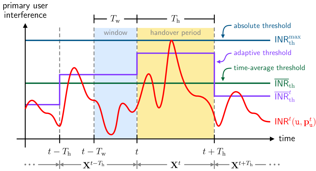
Figure 3: Combining a time-average constraint $\overline{\mathsf{INR}}_{\mathrm{th}}$ and an absolute constraint $\mathsf{INR}_{\mathrm{th}}^{\mathrm{max}}$ provides flexibility in secondary satellite selection while guaranteeing a certain level of protection to primary users.

$$g({\mathbf{X}}^{t},\lambda,\mu,\bm{\nu})=\sum_{n=1}^{{N_{\mathrm{G}}}}{\sum_{m=1}^{{N_{\mathrm{S}}}}{\left(c^{t}_{m,n}-\lambda\cdot\max_{{\mathtt{u}}\in\mathcal{U}}\,\overline{\mathsf{INR}}_{{T_{\mathrm{h}}}}^{t}({\mathtt{u}},{{\mathbf{p}}}_{\mathtt{u}};{{\mathbf{s}}}_{m},{{\mathbf{g}}}_{n})-\mu\cdot\max_{{\mathtt{u}}\in\mathcal{U},\tau\in\mathcal{T}}\mathsf{INR}^{\tau}({\mathtt{u}},{{\mathbf{p}}}_{\mathtt{u}};{{\mathbf{s}}}_{m},{{\mathbf{g}}}_{n})-\nu_{m}\right)}\cdot x^{t}_{m,n}}\\ +\lambda\cdot\overline{\mathsf{INR}}^{t}_{\mathrm{th}}+\mu\cdot\mathsf{INR}_{\mathrm{th}}^{\mathrm{max}}+\sum_{m=1}^{{N_{\mathrm{S}}}}\nu_{m}$$ (29)

$$\max_{{\mathbf{X}}^{t}} \sum_{m=1}^{N_{s}}{\left\{c_{m,n}^{t}-\lambda\cdot\max_{{\mathtt{u}}\in\mathcal{U}}\,\overline{\mathsf{INR}}_{{T_{\mathrm{h}}}}^{t}({\mathtt{u}},{{\mathbf{p}}}_{\mathtt{u}};{{\mathbf{s}}}_{m},{{\mathbf{g}}}_{n})-\mu\cdot\max_{{\mathtt{u}}\in\mathcal{U},\tau\in\mathcal{T}}\mathsf{INR}^{\tau}({\mathtt{u}},{{\mathbf{p}}}_{\mathtt{u}};{{\mathbf{s}}}_{m},{{\mathbf{g}}}_{n})-\nu_{m}\right\}}\cdot x_{m,n}^{t}\ \forall\ n$$ (32)

$$m^{\star}_{n}=\operatorname*{argmax}_{m=1,\dots,{N_{\mathrm{S}}}}{\left\{c_{m,n}^{t}-\lambda\cdot\max_{{\mathtt{u}}\in\mathcal{U}}\,\overline{\mathsf{INR}}_{{T_{\mathrm{h}}}}^{t}({\mathtt{u}},{{\mathbf{p}}}_{\mathtt{u}};{{\mathbf{s}}}_{m},{{\mathbf{g}}}_{n})-\mu\cdot\max_{{\mathtt{u}}\in\mathcal{U},\tau\in\mathcal{T}}\mathsf{INR}^{\tau}({\mathtt{u}},{{\mathbf{p}}}_{\mathtt{u}};{{\mathbf{s}}}_{m},{{\mathbf{g}}}_{n})-\nu_{m}\right\}}\ \forall\ n$$ (33)

 

III-B Problem Formulation

Having formulated a suitable time-averaged interference protection constraint, we now set our sights on optimizing the association made at handover time $t$, i.e., ${\mathbf{X}}^{t}$. In doing so, we assume the secondary system aims to maximize its own performance in terms of its capacity, though other measures could also be suitable. In this vein, let us define the aggregate capacity across secondary users in cluster ${{\mathbf{g}}}_{n}$ when served by secondary satellite ${{\mathbf{s}}}_{m}$ throughout the handover period $\mathcal{T}$ as

$$c_{m,n}^{t} \triangleq\sum_{\tau=t}^{t+{T_{\mathrm{h}}}-1}\!\!\sum_{{\mathtt{v}}\in\mathcal{V}_{n,\ell}}\log_{2}{\left(1+\gamma^{\tau}({\mathtt{v}},{{\mathbf{s}}}_{m},{{\mathbf{c}}}_{n,\ell})\right)}\cdot y^{\tau}_{m,n,\ell},$$ (27)

where $\gamma^{\tau}({\mathtt{v}},{{\mathbf{s}}}_{m},{{\mathbf{c}}}_{n,\ell})=\mathsf{SINR}^{\tau}({\mathtt{v}},{{\mathbf{s}}}_{m},{{\mathbf{c}}}_{n,\ell})\,\mathbbm{1}{\left[{{\mathbf{s}}}_{m}\in\mathcal{S}^{t}_{n}\right]}$, which captures the minimum elevation requirement in (3). Treating this notion of sum capacity as our objective, our association problem at handover time $t$ can be formulated by imposing the interference projection constraint derived before, along with aforementioned system constraints.

$$\max_{{\mathbf{X}}^{t}}\, \sum_{m=1}^{{N_{\mathrm{S}}}}\sum_{n=1}^{{N_{\mathrm{G}}}}c^{t}_{m,n}\cdot x^{t}_{m,n}$$ (28a)

$$\mathrm{s.t.~} \max_{{\mathtt{u}}\in\mathcal{U}}\sum_{m=1}^{{N_{\mathrm{S}}}}\sum_{n=1}^{{N_{\mathrm{G}}}}\overline{\mathsf{INR}}_{{T_{\mathrm{h}}}}^{t}({\mathtt{u}},{{\mathbf{p}}}_{\mathtt{u}};{{\mathbf{s}}}_{m},{{\mathbf{g}}}_{n})x_{m,n}^{t}\leq\overline{\mathsf{INR}}^{t}_{\mathrm{th}}$$ (28b)

$$\max_{\begin{subarray}{c}{\mathtt{u}}\in\mathcal{U}\\ \tau\in\mathcal{T}\end{subarray}}\sum_{m=1}^{{N_{\mathrm{S}}}}\sum_{n=1}^{{N_{\mathrm{G}}}}\mathsf{INR}^{\tau}({\mathtt{u}},{{\mathbf{p}}}^{t}_{\mathtt{u}};{{\mathbf{s}}}_{m},{{\mathbf{g}}}_{n})x_{m,n}^{t}\!\leq\!\mathsf{INR}_{\mathrm{th}}^{\mathrm{max}}$$ (28c)

$$\sum_{n=1}^{{N_{\mathrm{G}}}}x^{t}_{m,n}\leq 1\ \forall\ m$$ (28d)

$$\sum_{m=1}^{{N_{\mathrm{S}}}}x^{t}_{m,n}\leq 1\ \forall\ n$$ (28e)

$$x^{t}_{m,n}\in{\left\{0,1\right\}}\ \forall\ m,n$$ (28f)

Solving problem (28) at handover time $t$ would yield the secondary system satellite-cluster association ${\mathbf{X}}^{t}$ that maximizes the sum capacity throughout the handover period $[t,t+{T_{\mathrm{h}}})$ while ensuring the average and absolute interference inflicted upon any given primary user are constrained to some specified thresholds. Notice that maximizing the secondary system sum capacity amounts to choosing the association ${\mathbf{X}}^{t}$ that delivers high SINR to its users and yields lower received interference inflicted by the primary system. In other words, the optimal secondary satellite serving a given cluster of secondary users would likely be spatially separated from the primary satellites serving nearby primary users, in terms of both its own capacity and interference protection. It is important to note that, if the interference constraints are particularly strict, the secondary system may be unable to serve certain clusters during a given handover period. Such outage events are an undesired yet natural consequence of overly protective interference constraints.

III-C Lagrangian Relaxation and Subgradient Iterations

Problem (28) is a matching problem [40], known to be NP-hard [41]. In light of this, we solve it by relaxing inequality constraints (28b), (28c), and (28d) through Lagrangian relaxation [42]. This transforms the original problem into a dual problem which can be decomposed into smaller, independent subproblems that are easier to solve using dynamic programming. The Lagrangian multipliers can then be optimized via subgradient iteration [43], i.e., iteratively updated based on the violation of the original constraints.

Let ${\lambda}\in\mathbb{R}$, ${\mu}\in\mathbb{R}$, and $\bm{\nu}\in\mathbb{R}^{{N_{\mathrm{S}}}\times 1}$ be Lagrange multipliers and define $g({\mathbf{X}}^{t},{\lambda},\mu,\bm{\nu})$ as in (29). Due to the inequality constraints (28b), (28c), and (28d), we have

$$\max_{{\mathbf{X}}^{t}}\,g({\mathbf{X}}^{t},{\lambda},\mu,\bm{\nu})\geq\max_{{\mathbf{X}}^{t}}\,\sum_{m=1}^{{N_{\mathrm{S}}}}\sum_{n=1}^{{N_{\mathrm{G}}}}c^{t}_{m,n}\,x^{t}_{m,n},$$ (30)

for all $\lambda\geq 0$, $\mu\geq 0$, and $\bm{\nu}\geq\bm{0}$. The dual function $g(\lambda,\mu,\bm{\nu})$ is obtained by maximizing the Lagrangian over ${\mathbf{X}}^{t}$:

$$g(\lambda,\mu,\bm{\nu})\triangleq\max_{{\mathbf{X}}^{t}}\ g({\mathbf{X}}^{t};\lambda,\mu,\bm{\nu})$$ (31a)

$$\mathrm{s.t.~} \sum_{m}x_{m,n}^{t}\leq 1,\,\ x_{m,n}^{t}\in{\left\{0,1\right\}}.$$ (31b)

Note that Lagrangian relaxation with ${\left\{0,1\right\}}$ constraints in (31b) preserves the optimality of the original problem [42].

Given the Lagrangian multipliers, the dual function (31a) can be decomposed into independent cluster-level subproblems as in (32). Thus, at each cluster $n$, we find the optimal satellite $m_{n}^{\star}$ satisfying (33): if $m=m^{\star}_{n}$ we have $x_{m,n}^{t}=1$, otherwise $x_{m,n}^{t}=0$, for each $n$. The Lagrangian multipliers can then be optimized by subgradient iteration [43], and the dual problem $\min_{\lambda\geq 0,\mu\geq 0,\bm{\nu}\geq\bm{0}}\,g(\lambda,\mu,\bm{\nu})$ is optimized to provide bounds on the original problem’s solution [42]. This concludes our proposed secondary satellite selection mechanism, which we thoroughly assess in the next section.

IV Evaluating Our Secondary
Satellite Selection Mechanism

To conduct a thorough and relevant analysis on the in-band coexistence of two dense LEO satellite communication systems under our proposed selection mechanism, we consider two preeminent commercial systems at $20$ GHz: Starlink as the primary and Kuiper as the secondary system; this is motivated by the fact that Starlink has priority rights over Kuiper to transmit downlink in the $19.7$–$20.2$ GHz band. We simulate the Starlink and Kuiper constellations in a Walker-Delta fashion [44], using Matlab’s Aerospace Toolbox [45], based on the orbital parameters detailed in Table I and Table II, which are extracted from public filings [30, 46, 47]. The total numbers of primary and secondary satellites are correspondingly ${N_{\mathrm{P}}}=6900$ and ${N_{\mathrm{S}}}=3236$. Primary and secondary satellite locations are sampled every $0.1$ sec in simulation. Although ${T_{\mathrm{h}}}$ and ${T_{\mathrm{w}}}$ were defined in the previous section in units of time samples, they are expressed here in seconds to provide a more meaningful interpretation.

TABLE I: SpaceX’s Starlink Constellation Parameters [46, 47]

Altitude	Inclination	Planes	Satellites/Plane	Total No. Satellites
$540$ km	$53.2^{\circ}$	$72$	$22$	$1584$
$550$ km	$53^{\circ}$	$72$	$22$	$1584$
$560$ km	$97.6^{\circ}$	$4$	$43$	$172$
$560$ km	$97.6^{\circ}$	$6$	$58$	$348$
$570$ km	$70^{\circ}$	$36$	$20$	$720$
$530$ km	$33^{\circ}$	$28$	$89$	$2492$

TABLE II: Amazon’s Project Kuiper Constellation Parameters [30]

Altitude	Inclination	Planes	Satellites/Plane	Total No. Satellites
$590$ km	$33^{\circ}$	$28$	$28$	$784$
$610$ km	$42^{\circ}$	$36$	$36$	$1296$
$630$ km	$51.9^{\circ}$	$34$	$34$	$1156$

Each satellite is equipped with 64$\times$64 phased array antennas capable of generating multiple spot beams to serve ground users, delivering a maximum transmit beam gain of $36$ dBi, and the receive antenna of ground users are modeled with 32$\times$32 phased array antennas. Based on the resulting $-3$ dB transmit beam contours, the radius of ground cells is approximately $10$ km, and we consider ${N_{\mathrm{G}}}=10$ clusters as illustrated in Figure 2, each comprised with ${N_{\mathrm{C}}}=127$ ground cells. These values are on par with their public filings [36, 48]. We evaluate coexistence of the two satellite systems for a various number of spot beams per satellite, exploring four configurations: 8, 16, 24, and 32 beams [32, 33]. We consider a frequency reuse factor of three, following [30]. To assess a worst-case interference scenario, we assume that both the primary and secondary systems share the same ground cell and cluster deployment with overlapping cell centers, and users are uniformly distributed across all ground cells. To comply with power flux density regulations [31] set by regulatory authorities such as the FCC, a simple transmit power control mechanism is implemented at each satellite based on path distance and elevation angle. Specifically, the maximum EIRP provided in Table III applies only to satellites operating at nadir at the highest altitude in the constellation. Despite the high velocity of LEO satellites, which induces significant Doppler effects, we do not explicitly account for such in our analysis, as they are accurately estimated and compensated for in practice based on satellite orbits and user locations [49, 50]. Key simulation parameters are summarized in Table III, all of which are based on public filings and 3GPP specifications [36, 48, 51].

TABLE III: Key Simulation Parameters [36, 48, 51]

Primary and Secondary Satellites
Tx. Antenna Array	No. Antennas	64$\times$64
	3 dB Beamwidth	$1.6^{\circ}$
	Max. Beam Gain	$36$ dBi
Max. EIRP	Primary Sat.	$-54.3$ dBW/Hz
	Secondary Sat.	$-53.3$ dBW/Hz
Primary and Secondary Ground Users
Rx. Antenna Array	No. Antennas	32$\times$32
	Max. Beam Gain	$30$ dBi
	3 dB Beamwidth	$3.2^{\circ}$
Noise Power Spectral Density		$-174$ dBm/Hz
Noise Figure		$1.2$ dB

IV-A Satellite-to-Cluster Association of Primary System

A natural starting point in our evaluation is to assess system performance when the secondary system makes no attempt to protect the primary system. It is thus necessary to define the association policies initially employed by both systems. (Afterwards, the secondary system association will be governed by our proposed satellite selection mechanism.) In this vein, we consider two plausible handover policies: highest elevation (HE) and maximum contact time (MCT) [52]. Under the HE policy, a given satellite system selects the satellite with the highest elevation angle relative to the cluster it aims to serve. In this case, the handover period is set to ${T_{\mathrm{h}}}=15$ sec, coinciding with that observed in Starlink [38]. In contrast, the MCT policy prioritizes the satellite that offers the longest visible time above the minimum elevation angle. In this approach, a handover is initiated when the serving satellite is expected to descend below the minimum elevation angle, transitioning to the satellite that provides the longest remaining visibility. In applying these policies cluster-by-cluster, the prioritization numbering shown in Figure 2 is used to dictate the order in which this association is carried out. This can capture prioritizing denser areas for higher capacity. Under the HE policy, if a particular satellite is that with the highest elevation across multiple clusters, it is assigned to the highest priority cluster. This prioritization is analogously applied to the MCT policy.

IV-B Independent Operation of the Two Systems

We begin our evaluation by assessing the performance when the secondary system operates without any attempt to protect the primary system. To do so, at each time step in our simulation (under a 0.1 sec resolution), we compute the INR and SINR of both primary and secondary users after performing the aforementioned satellite-to-cluster association policies. Note that the only interference considered, for the sake of clarity, is that inflicted by the other system. In reality, intra-system interference would also be present but may be carefully controlled by each constellation separately, and we therefore omit it to focus exclusively on inter-system interference.

We examine the primary user INR for a various number of spot beams per satellite and assess performance under the aforementioned handover policies of HE and MCT. Figure 4 depicts the cumulative distribution function (CDF) of the INR across primary users and across time, representing the aggregate interference from all active satellites and spot beams of the secondary system, i.e., $\mathsf{INR}^{t}({\mathtt{u}},{{\mathbf{p}}})$ as defined in (15). Solid lines in the figure represent scenarios where the secondary system adopts the same handover policy as the primary system, and dotted lines indicate cases where the secondary system differs in its handover policy, using MCT. We can see that adopting a different handover policy at the secondary system slightly reduces the INR inflicted onto primary users. This marginal improvement is presumably due to improved spatial separation of the selected primary and secondary satellites, as MCT naturally tends to select satellites earlier in their overhead pass and thus closer to the horizon, whereas HE selects those closer to nadir.

Takeaway 1: Independent operation of the two systems leads to prohibitively high interference.

As evident in Figure 4, even with only $N_{\mathrm{B}}=8$ spot beams per satellite, there is substantial interference inflicted onto primary users a non-negligible fraction of the time. Referencing an INR threshold of $-12.2$ dB, as widely employed by the ITU [27, 28], we can see that around $20\%$ of primary users would exceed this interference threshold. This naturally worsens as the number of spot beams increases. With $N_{\mathrm{B}}=32$, this INR threshold is exceeded for around $50\%$ of users, regardless of the policies employed by the two independent systems. These results motivate the need for mechanisms to explicitly protect primary users, in order to facilitate a healthy coexistence paradigm between two dense LEO satellite constellations.

IV-C Coexistence Under Our Proposed Approach

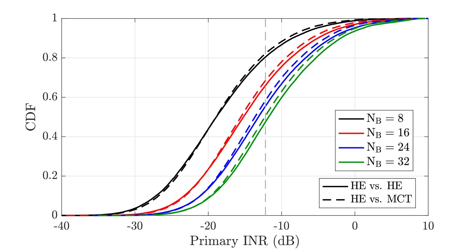
Figure 4: The CDF of INR across primary users and across time for a various number of spot beams and handover policies. The INR at approximately $20\%$ of primary users exceeds $-12.2$ dB when $N_{\mathrm{B}}=8$, further increasing with $N_{\mathrm{B}}$. The upper tail motivates the need for the secondary system to explicitly protect primary users.

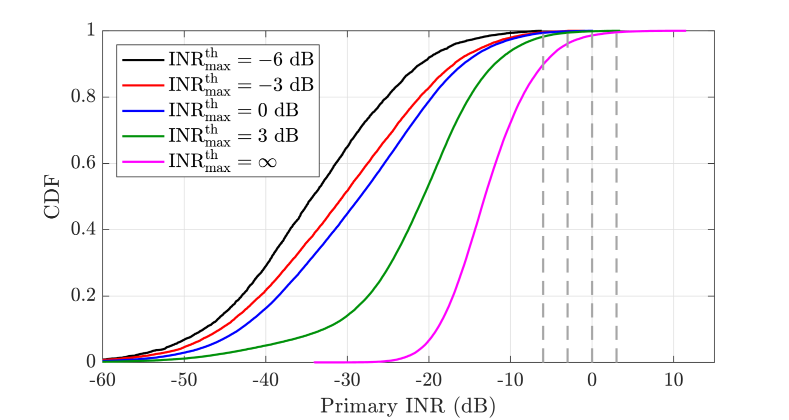
Figure 5: The CDF of the primary user INR (across users and time) for various $\mathsf{INR}_{\mathrm{th}}^{\mathrm{max}}$ values under our proposed approach. The average INR threshold $\overline{\mathsf{INR}}_{\mathrm{th}}$ is set to $-6$ dB, with ${T_{\mathrm{h}}}=15$ sec and ${T_{\mathrm{w}}}=10$ sec.

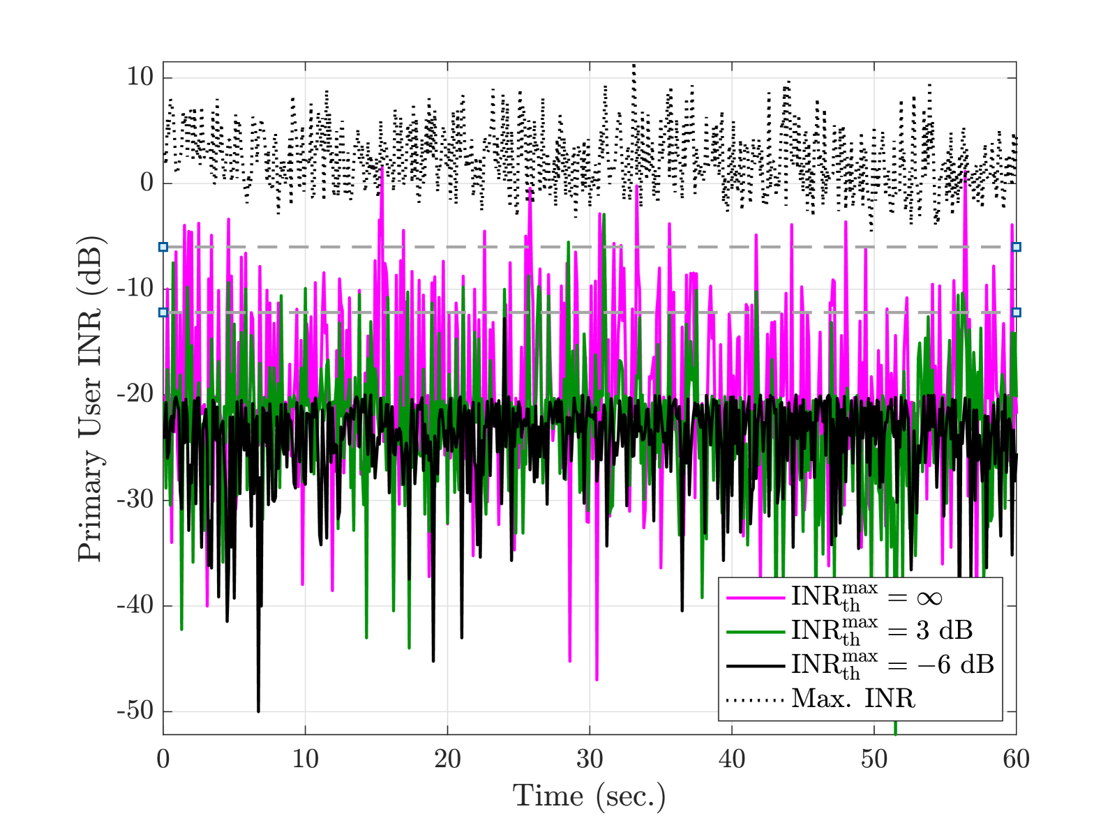
Figure 6: Instantaneous INR experienced by a single primary ground user during a $60$-sec period under our proposed scheme for various absolute thresholds $\mathsf{INR}_{\mathrm{th}}^{\mathrm{max}}$. The dotted line indicates the maximum INR across all primary ground users throughout the handover period. The time-average INR constraint is set to $\overline{\mathsf{INR}}_{\mathrm{th}}=-6$ dB, with ${T_{\mathrm{h}}}=15$ sec and ${T_{\mathrm{w}}}=10$ sec.

Having motivated the need for explicit protection mechanisms, we now turn our attention toward assessing our proposed approach described in Section III, with $N_{\mathrm{B}}=16$, the typical number of spot beams per satellite in Starlink [33]. In Figure 5, we plot the CDF of the primary INR (across users and time) when employing our protection mechanism with absolute protection thresholds $\mathsf{INR}_{\mathrm{th}}^{\mathrm{max}}$, where the time-average threshold has been set to $\overline{\mathsf{INR}}_{\mathrm{th}}=-6$ dB. The black line with $\mathsf{INR}_{\mathrm{th}}^{\mathrm{max}}=-6$ dB is thus equivalent to the strict protection constraint described in (18). In this case, we can see that indeed the primary INR never exceeds $-6$ dB and is orders of magnitude below $-6$ dB most of the time. Upon increasing the absolute threshold $\mathsf{INR}_{\mathrm{th}}^{\mathrm{max}}$, the distribution shifts rightward but still lies well below $-6$ dB most of the time. The upper tail exceeds $-6$ dB, however, as a consequence of the flexibility provided by increasing $\mathsf{INR}_{\mathrm{th}}^{\mathrm{max}}$. Since the time-average threshold remains at $\overline{\mathsf{INR}}_{\mathrm{th}}=-6$ dB, the distribution is nonetheless constrained to remain mostly below $-6$ dB. We can see that, even with $\mathsf{INR}_{\mathrm{th}}^{\mathrm{max}}=3$ dB, the primary INR only exceeds $-6$ dB about 3% of the time. If an instantaneous INR of $-12.2$ dB were used to define protection, we can see that a time-average threshold of $\overline{\mathsf{INR}}_{\mathrm{th}}=-6$ dB does meet this a high percentage of the time for a suitably chosen $\mathsf{INR}_{\mathrm{th}}^{\mathrm{max}}$. This illustrates that, by pairing an absolute interference constraint with a time-averaged one, our proposed protection mechanism is capable of meeting more flexible yet still protective operating points for appropriately chosen $\overline{\mathsf{INR}}_{\mathrm{th}}$ and $\mathsf{INR}_{\mathrm{th}}^{\mathrm{max}}$. Soon, we will show that this flexibility greatly improves secondary system performance.

Thus far, we have evaluated the performance of our proposed approach in terms of the CDF of INR across all primary users and time. To gain clearer insight into our approach’s behavior, we now examine the instantaneous INR of a single primary user over 60 sec (four handover periods). This is shown in Figure 6 for various absolute thresholds $\mathsf{INR}_{\mathrm{th}}^{\mathrm{max}}$ with the time-averaged INR constraint $\overline{\mathsf{INR}}_{\mathrm{th}}=-6$ dB, when ${T_{\mathrm{w}}}=10$ sec and ${T_{\mathrm{h}}}=15$ sec. Notice that with $\mathsf{INR}_{\mathrm{th}}^{\mathrm{max}}=-6$ dB, the INR at this particular user remains well below the time-average constraint of $-6$ dB throughout the entire handover period; there is only one narrow spike that approaches $-12.2$ dB. Increasing to $\mathsf{INR}_{\mathrm{th}}^{\mathrm{max}}=3$ dB leads to occasional, short-lived spikes in INR exceeding $-12.2$ dB. However, this particular user only sees a worst-case INR around $-5$ dB and INR only exceeds the time-average threshold of $\overline{\mathsf{INR}}_{\mathrm{th}}=-6$ dB twice in this minute-long duration. When $\mathsf{INR}_{\mathrm{th}}^{\mathrm{max}}=\infty$, INR far more frequently exceeds both $-12.2$ dB and $-6$ dB and occasionally approaches or exceeds $0$ dB. For context, we have included the maximum INR across users when $\mathsf{INR}_{\mathrm{th}}^{\mathrm{max}}=\infty$ in the dotted line, which illustrates that there are indeed users across the network that do incur prohibitively high INR at virtually any given time. However, the interference profile of this single user suggests that high INR at any one user is typically short-lived. This motivates us to quantify the fraction of primary users that see high INR at any given time next, but let us first draw the following conclusions.

Takeaway 2: For a fixed satellite association, primary user INR can fluctuate rapidly and widely throughout a handover period.

This can be attributed to the many satellites and beams that comprise this complex, time-varying interference setting, further illustrating the challenges in meeting a strict protection constraint throughout an entire handover period. Furthermore, increasing (or even removing) the absolute INR constraint does not necessarily result in all users seeing extremely high INR. As we will see, this relaxation can greatly improve utilization of the secondary system by allowing it to select satellites which would otherwise be unable to serve particularly problematic primary users.

While raw primary user INR is certainly important, it is only one component in assessing coexistence. For this reason, we introduce two metrics to more straightforwardly assess coexistence under our proposed satellite selection mechanism:

• the violation rate, defined as the fraction of primary users whose instantaneous INR exceeds the time-average threshold $\overline{\mathsf{INR}}_{\mathrm{th}}$, i.e., $\frac{1}{|\mathcal{U}|}\sum_{{\mathtt{u}}\in\mathcal{U}}\mathbbm{1}{\left[\mathsf{INR}^{t}({\mathtt{u}},{{\mathbf{p}}})>\overline{\mathsf{INR}}_{\mathrm{th}}\right]}$;

• secondary system utilization, defined as the fraction of secondary ground users actively served by the secondary system, i.e., $\frac{1}{{N_{\mathrm{G}}}}\sum_{m=1}^{N_{\mathrm{S}}}\sum_{n=1}^{N_{\mathrm{G}}}x^{t}_{m,n}$.

We seek a low violation rate and a high utilization for healthy coexistence, both of which depend on the time-average constraint $\overline{\mathsf{INR}}_{\mathrm{th}}$ and the absolute constraint $\mathsf{INR}_{\mathrm{th}}^{\mathrm{max}}$. Note that the violation rate will be zero when $\mathsf{INR}_{\mathrm{th}}^{\mathrm{max}}=\overline{\mathsf{INR}}_{\mathrm{th}}$, but this may lead to poor utilization for strict $\mathsf{INR}_{\mathrm{th}}^{\mathrm{max}}$, as the secondary system may be unable to serve its users while guaranteeing protection, forcing it to leave some clusters un-served in a given handover period.

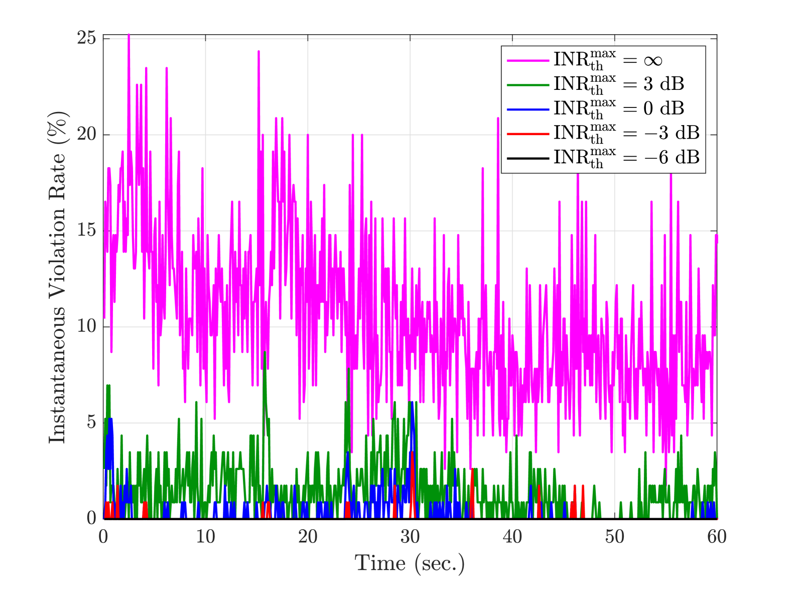
Figure 7: Instantaneous violation rate (across primary users) for various absolute thresholds $\mathsf{INR}_{\mathrm{th}}^{\mathrm{max}}$, where $\overline{\mathsf{INR}}_{\mathrm{th}}=-6$ dB, ${T_{\mathrm{h}}}=15$ sec, and ${T_{\mathrm{w}}}=10$ sec.

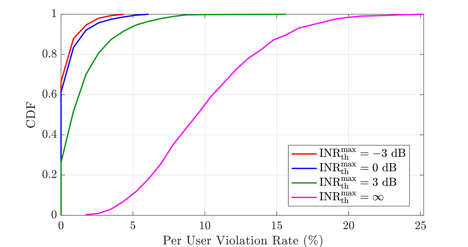
Figure 8: The CDF of violation rate per primary user (across time) for various absolute thresholds $\mathsf{INR}_{\mathrm{th}}^{\mathrm{max}}$, where $\overline{\mathsf{INR}}_{\mathrm{th}}=-6$ dB, ${T_{\mathrm{h}}}=15$ sec, and ${T_{\mathrm{w}}}=10$ sec.

In Figure 7, we plot the instantaneous violation rate for various $\mathsf{INR}_{\mathrm{th}}^{\mathrm{max}}$ across the same 60-sec period of Figure 6. We can see that for $\mathsf{INR}_{\mathrm{th}}^{\mathrm{max}}=\infty$, around $10$–$15$% of users consistently see interference that exceeds $\overline{\mathsf{INR}}_{\mathrm{th}}=-6$ dB. This violation rate exceeds $25$% at its peak and dips below $5$% at its lowest. When setting $\mathsf{INR}_{\mathrm{th}}^{\mathrm{max}}=3$ dB, the violation rate drastically drops to below $5$% the vast majority of the time. This trend continues as $\mathsf{INR}_{\mathrm{th}}^{\mathrm{max}}$ is decreased further, intuitively reaching $0$% when $\mathsf{INR}_{\mathrm{th}}^{\mathrm{max}}=\overline{\mathsf{INR}}_{\mathrm{th}}=-6$ dB.

Further exploring violation, let us examine how frequently each individual primary user experiences violation. We define the per-user violation rate as the fraction of time in which a primary user’s INR exceeds $\overline{\mathsf{INR}}_{\mathrm{th}}$. Figure 8 shows the CDF of the per-user violation rate across all primary users for various absolute thresholds $\mathsf{INR}_{\mathrm{th}}^{\mathrm{max}}$, given $\overline{\mathsf{INR}}_{\mathrm{th}}=-6$ dB. With $\mathsf{INR}_{\mathrm{th}}^{\mathrm{max}}\leq 3$ dB, we see fairly encouraging results: over 90% of users experience violations less than 5% of the time. For $\mathsf{INR}_{\mathrm{th}}^{\mathrm{max}}=\infty$, all users see violations much more frequently. Still, it is encouraging to see that more than half of users see violations less than 10% of the time. Moreover, we can see that a worst-case user sees violations at most 25% of the time.

To shed light on utilization along with violation, Table IV summarizes both for various time-average thresholds $\mathsf{INR}_{\mathrm{th}}$ and absolute thresholds $\mathsf{INR}_{\mathrm{th}}^{\mathrm{max}}$. Let us first recognize that, when $\overline{\mathsf{INR}}_{\mathrm{th}}=\mathsf{INR}_{\mathrm{th}}^{\mathrm{max}}=-12.2$ dB, which corresponds to a conventional strict protection constraint as described in (18), there is no violation, but this leads to an average utilization of merely $3.47$%. Similarly, when $\overline{\mathsf{INR}}_{\mathrm{th}}=\mathsf{INR}_{\mathrm{th}}^{\mathrm{max}}=-6$ dB, utilization is only $22.16$%. The average violation naturally increases as $\mathsf{INR}_{\mathrm{th}}^{\mathrm{max}}$ is relaxed but only modestly so. Average utilization, on the other hand, increases substantially to over $80$% with $\overline{\mathsf{INR}}_{\mathrm{th}}=-12.2$ dB and to $100$% for $\overline{\mathsf{INR}}_{\mathrm{th}}=-6$ dB.

Takeaway 3: Trading off minor increases in violation rate for major increases in utilization rate is the key advantage of our proposed protection constraint.

With a conventional strict constraint, the secondary system must make substantial sacrifices in utilization to meet extremely low INR thresholds across all users throughout entire handover periods. With our approach, however, short-lived spikes in INR are tolerated in order to enhance secondary system utilization, while still ensuring a certain level of protection is maintained at all users throughout handover periods. This balance is crucial for effective coexistence.

TABLE IV: Utilization and Violation ($\%$)

	$\overline{\mathsf{INR}}_{\mathrm{th}}=-12.2$ dB		$\overline{\mathsf{INR}}_{\mathrm{th}}=-6$ dB
$\mathsf{INR}_{\mathrm{th}}^{\mathrm{max}}$	Utilization	Violation	Utilization	Violation
$-12.2$ dB	3.47	0	N/A	N/A
$-6$ dB	22.16	1.34	22.16	0
$-3$ dB	53.44	3.70	56.45	0.47
$0$ dB	66.05	4.55	73.75	0.63
$3$ dB	84.76	10.09	93.92	1.79
$\infty$	87.41	13.07	100	10.20

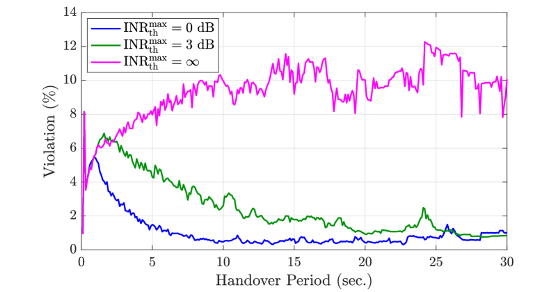
(a) Average violation rate.

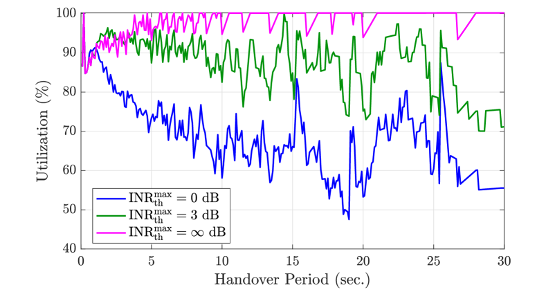
(b) Average secondary system utilization.

Figure 9: Average violation and utilization rates as a function of handover period ${T_{\mathrm{h}}}$ for various $\mathsf{INR}_{\mathrm{th}}^{\mathrm{max}}$, when $\overline{\mathsf{INR}}_{\mathrm{th}}=6$ dB and ${T_{\mathrm{w}}}=10$ sec. When $\mathsf{INR}_{\mathrm{th}}^{\mathrm{max}}$ is high, increasing ${T_{\mathrm{h}}}$ tends to increase utilization, since it provides longer durations to average out spikes in INR, but this leads to a higher violation rate. When $\mathsf{INR}_{\mathrm{th}}^{\mathrm{max}}$ is low, increasing ${T_{\mathrm{h}}}$ tends to decrease utilization since the secondary system cannot meet the protection without putting some clusters into outage; this naturally decreases the violation rate.

Let us now examine Figure 9a, which depicts average violation rate as a function of the handover period ${T_{\mathrm{h}}}$, for $\overline{\mathsf{INR}}_{\mathrm{th}}=-6$ dB and various $\mathsf{INR}_{\mathrm{th}}^{\mathrm{max}}$. We can see that the violation rate is generally lower for a stricter absolute protection constraint $\mathsf{INR}_{\mathrm{th}}^{\mathrm{max}}$, but we can observe two noteworthy trends beyond this. First, when $\mathsf{INR}_{\mathrm{th}}^{\mathrm{max}}=\infty$, the violation rate tends to increase with handover period ${T_{\mathrm{h}}}$. This can be explained by the fact that a longer handover period allows the system to tolerate (average out) high spikes in INR while still meeting the time-average protection constraint. Even when $\mathsf{INR}_{\mathrm{th}}^{\mathrm{max}}=\infty$, the violation rate caps at about $12\%$. The second trend can be stated as, when $\mathsf{INR}_{\mathrm{th}}^{\mathrm{max}}$ is lower, violation rate tends to decrease as the handover period is increased. This is because, for strict absolute thresholds $\mathsf{INR}_{\mathrm{th}}^{\mathrm{max}}$, it is more difficult for the secondary satellite system to meet the constraint; this exacerbates as the handover period is increased, since the same association is used throughout the entire handover period. Consequently, the secondary system is more often incapable of serving some clusters when $\mathsf{INR}_{\mathrm{th}}^{\mathrm{max}}$ is low, which naturally reduces the violation rate.

This can be confirmed from Figure 9b, which shows the corresponding secondary system utilization as a function of handover period. We can see that the secondary system utilization is heavily impacted by the handover period for strict $\mathsf{INR}_{\mathrm{th}}^{\mathrm{max}}$, as utilization can drop to around $50\%$ for a handover period of ${T_{\mathrm{h}}}\approx 18$ sec. Again, this is because the secondary system is incapable of meeting such a strict absolute constraint across all users throughout long handover periods and is forced to leave certain clusters in outage. When $\mathsf{INR}_{\mathrm{th}}^{\mathrm{max}}$ is increased, utilization increases thanks to the relaxed protection constraint. However, even in the most relaxed case when $\mathsf{INR}_{\mathrm{th}}^{\mathrm{max}}=\infty$, there are select cases where the time-average constraint cannot be met. Furthermore, one can notice that when the handover period ${T_{\mathrm{h}}}$ is made small (which relaxes the absolute constraint), the utilization still falls short of 100% and is in fact not maximized. This can be best explained by the fact that a small ${T_{\mathrm{h}}}$ results in a more restrictive time-average constraint, as a shorter handover period offers less time to average out spikes in interference. When ${T_{\mathrm{h}}}$ is increased, more frequent and/or higher spikes in interference can be tolerated, as there is more time to average them out and meet the time-average constraint $\overline{\mathsf{INR}}_{\mathrm{th}}$. Thus, to maximize secondary system utilization under a given $\overline{\mathsf{INR}}_{\mathrm{th}}$, $\mathsf{INR}_{\mathrm{th}}^{\mathrm{max}}$ and ${T_{\mathrm{h}}}$ should both be high.

Takeaway 4: Optimizing coexistence entails careful selection of a number of parameters.

Given the complexity of this interference scenario, it is difficult to state a one-size-fits-all solution. With our proposed framework, however, multiple parameters can be tuned to reliably arrive at a satellite selection mechanism which meets an acceptable violation rate while maximizing utilization. Regulators will play a pivotal role in defining violation rates and worst-case INR that are acceptable in this context. Beyond this, the rate at which the secondary system can perform handovers will also have decisive impact on its ability to coexist with the primary system.

V Coexistence Under Uncertainty
about the Primary System

Until now, we have implicitly assumed that the secondary system has perfect knowledge of the primary system association at any given time. This assumption may be sound in cases where the two systems communicate with one another (or through a third party, such as a regulator), but this is not expected nor mandated in today’s LEO landscape. Motivated by this, this section presents and assesses schemes which use DL to learn the primary system’s association policy. More specifically, we propose using secondary ground users to measure the received power from primary satellites, which can then be used to infer the primary serving satellites over time in a given area. These inferred primary serving satellites are then used to train a centralized DL model, which can then be used to forecast the primary satellite which serves a given location at any point in the future, based solely on the primary satellite locations—which is publicly available.

Let the input of our DL model be ${\mathbf{I}}={\left\{\mathcal{P}^{t}_{\mathcal{G}},\mathcal{G},\mathcal{E}^{t}\right\}}$, comprised of the primary available satellite locations at time $t$, the locations of all cluster centers, and the elevation angles of all available satellites with respect to each cluster at time $t$. The output of the DL model $\hat{{\mathbf{Y}}}=f({\mathbf{I}};\bm{\theta})\in\mathbb{R}^{{N_{\mathrm{G}}}}$ represents the index of the estimated primary serving satellite for each cluster, where $f(\cdot;\bm{\theta})$ is a learnable function defined by the DL model’s parameters $\bm{\theta}$. To compare the effectiveness of different DL models, we evaluated a single-layer (1L) perceptron, a three-layer (3L) multilayer perceptron (MLP), and an attention-based network. For the perceptron models, we use the scaled exponential linear unit (SELU) [53] as the activation function to enable self-normalization with a hidden size of 2048. Training data was generated by simulating the primary system’s satellite-to-cluster associations using Starlink’s constellation over the considered geographical area in Figure 2, using all of the same simulation parameters described in the previous section.

Table V presents the test accuracy of the considered DL models for each handover policy. Note that the model is not provided any explicit information about the primary system’s handover policy, as this is what it must learn. Accuracy is computed as the percentage of clusters (averaged over time) for which the model correctly predicts their serving primary satellites. The results indicate that the three DL models have difficulty in precisely identifying the primary serving satellites, achieving accuracies that range from about $51$–$67\%$. This suggests that learning even fairly simple association policies like HE and MCT is a more complex task than it may appear. Tackling this problem more extensively in dedicated work would thus make a valuable contribution.

On the other hand, given that the number of available satellites ranges from approximately $20$ to $25$ at each time instance, our learning algorithm shows promising results by correctly identifying the serving satellite for at least five out of the ten clusters. Although “$5$ out of $10$ correct” may seem like modest accuracy, the ample combinatorial possibilities in assigning a unique satellite to each of the 10 clusters indicate that this accuracy is still noteworthy. Additionally, the table provides accuracy metrics when predicting the top three or top five potential serving satellites, with performance for top-5 easily exceeding $90\%$. The implications of the DL models’ accuracy will be further evaluated in the context of primary and secondary satellite system coexistence in the following.

TABLE V: Test Data Accuracy of Various DL Models ($\%$)

Policy	DL Model	Top-$1$	Top-$3$	Top-$5$
HE	1L Perceptron	$57.66$	$88.21$	$95.26$
	3L MLP	$55.75$	$86.95$	$95.19$
	Attention	$51.21$	$83.52$	$92.27$
MCT	1L Perceptron	$60.86$	$88.83$	$96.07$
	3L MLP	$67.12$	$91.34$	$97.01$
	Attention	$57.94$	$86.72$	$94.78$

TABLE VI: Violation/Utilization Rate (each in $\%$) of $\overline{\mathsf{INR}}_{\mathrm{th}}$
(${T_{\mathrm{w}}}=10$ sec, ${T_{\mathrm{h}}}=15$ sec, $\mathsf{INR}_{\mathrm{max}}=\infty$)

$\overline{\mathsf{INR}}_{\mathrm{th}}$	True Sat.	Top-$1$	Top-$3$	Top-$5$
$-12.2$ dB	$13.07$/$87.41$	$15.74$/$42.53$	$2.13$/$26.04$	$2.24$/$14.03$
$-10$ dB	$12.91$/$92.04$	$13.63$/$87.19$	$2.63$/$32.19$	$1.84$/$20.03$
$-6$ dB	$10.22$/$100$	$10.71$/$98.53$	$3.81$/$46.02$	$0.71$/$24.04$
$0$ dB	$1.71$/$100$	$1.83$/$100$	$1.92$/$98.01$	$1.34$/$80.04$

The coexistence performance of the secondary system, based on the inferred primary system’s satellite-to-cluster association using a single-layer (1L) perceptron, is presented in Table VI, which reports utilization and violation metrics for various $\overline{\mathsf{INR}}_{\mathrm{th}}$ values. Despite the modest prediction accuracy being below $60\%$ (Table V), both utilization and violation metrics remain close to those obtained using true primary association data, except in the case of $\overline{\mathsf{INR}}_{\mathrm{th}}=-12.2$ dB. Specifically, when $\overline{\mathsf{INR}}_{\mathrm{th}}=-10$ dB, the utilization of the secondary system under the top-1 estimate is approximately $5\%$ lower than that obtained with true data, while the violation increases by less than $2\%$. These results indicate that, under a strict average threshold of $-12.2$ dB, a single violation due to an incorrect primary satellite estimate can disproportionately impact the association, highlighting an opportunity for further improvements of primary satellite prediction. However, with a more relaxed constraint, the inferred primary association data using the simple 1L perceptron enables performance comparable to that achieved with true data.

On the other hand, despite top-3 and top-5 estimates exhibiting a high prediction accuracy, notable reduction in utilization and violation is observed when the secondary system relies on the top-3 or top-5 estimates. This indicates that the secondary system overly protects the primary system and excessively refrain from assigning satellites to its clusters.

Takeaway 5: Leveraging DL models can facilitate the coexistence of dense LEO satellite systems.

The primary system’s satellite-to-cluster association can be estimated using a DL model by capturing spatial relationships and temporal patterns within the data. These patterns are influenced by satellite locations, handover policies, and cluster-specific priorities. A simple single-layer (1L) perceptron can achieve a modest accuracy in estimating this association. While high learning accuracy is not strictly necessary, even a moderate level of accuracy can effectively support the secondary system’s operation under a relaxed average INR constraint. However, under a strict constraint, this modest accuracy can significantly impact performance, emphasizing the need for more sophisticated learning models.

VI Conclusion and Future Directions

This work investigates the in-band coexistence of two dense LEO satellite communication systems through the lens of two leading commercial entities: SpaceX’s Starlink as the primary system and Amazon’s Project Kuiper as the secondary system. To enable coexistence, we propose a practical mechanism that strategically selects secondary serving satellites to maximize the secondary system capacity while guaranteeing protection to primary ground users. In doing so, we formulate a novel interference protection constraint that combines an absolute interference threshold and a time-averaged threshold, which provides flexibility in trading off interference violation rate for system utilization. We use Lagrangian relaxation and subgradient methods to solve our satellite selection problem and thoroughly evaluate performance through high-fidelity simulation based on public FCC filings and technical specifications.

Results show that independent operation of Starlink and Kuiper leads to prohibitively high interference, motivating the need for mechanisms such as ours that explicitly ensure protection. However, we observe that a conventional absolute protection constraint leads to either under-utilization of the secondary system or high interference at the primary users. With our proposed scheme and novel protection constraints, however, utilization and protection can be better balanced by tolerating infrequent, short-lived spikes in interference. This allows the primary and secondary systems to both enjoy high capacity while coexisting alongside one another. Finally, we demonstrated the potential use of DL techniques to infer the primary satellite associations at any given time based purely on the knowledge of overhead satellites, which can then be used by our proposed scheme to find near-optimal secondary satellite associations to enable coexistence.

A number of valuable directions are motivated by this work, including more extensively exploring DL techniques to improve the estimation of the primary system’s satellite-to-cluster association. Additionally, it would be valuable to consider cases where there is limited communication/coordination between the primary and secondary systems. Another promising direction is to investigate the coexistence of three or more satellite constellations, extending our analysis to more complex multi-system scenarios.

References

- [1] S. Chen, S. Sun, and S. Kang, “System integration of terrestrial mobile communication and satellite communication —the trends, challenges and key technologies in B5G and 6G,” China Commun., vol. 17, no. 12, pp. 156–171, Dec. 2020.
- [2] M. Sheng et al., “6G service coverage with mega satellite constellations,” China Commun., vol. 19, no. 1, pp. 64–76, Jan. 2022.
- [3] X. Lin et al., “On the path to 6G: Embracing the next wave of low Earth orbit satellite access,” IEEE Commun.Mag., pp. 36–42, Dec. 2021.
- [4] J. Heo et al., “MIMO satellite communication systems: A survey from the PHY layer perspective,” IEEE Commun. Surv. Tut., Jul. 2023.
- [5] J. C. McDowell. Jonathan’s space report. Oct. 2023. [Online]. Available: https://planet4589.org/space/con/star/stats.html
- [6] Report and Order and Further Notice of Proposed Rulemaking. FCC, Washington, DC, USA, Mar. 2023. [Online]. Available: https://docs.fcc.gov/public/attachments/DOC-392201A1.pdf
- [7] S. K. Sharma, S. Chatzinotas, and B. Ottersten, “Satellite cognitive communications: Interference modeling and techniques selection,” in Adv. Sat. Multimedia Sys. Conf. and Signal Process. Space Commun. Workshop, Oct. 2012, pp. 111–118.
- [8] M. Jia et al., “Broadband satellite-terrestrial communication systems based on cognitive radio toward 5G,” IEEE Wireless Commun., vol. 23, no. 6, pp. 96–106, Dec. 2016.
- [9] J. Hu et al., “Energy-efficient cooperative spectrum sensing in cognitive satellite terrestrial networks,” IEEE Access, pp. 161 396–161 405, 2020.
- [10] Study on New Radio (NR) to support non-terrestrial networks (NTN). Technical Report 38.811, v.15.3.0, 3GPP, Jul. 2020.
- [11] Y.-C. Liang et al., “Realizing intelligent spectrum management for integrated satellite and terrestrial networks,” J. Commun. Inf. Netw., vol. 6, no. 1, pp. 32–43, Mar. 2021.
- [12] G. Ding et al., “Spectrum inference in cognitive radio networks: Algorithms and applications,” IEEE Communs. Surv. Tut., pp. 150–182, Sep. 2017.
- [13] X. Zhou, M. Sun, G. Y. Li, and B.-H. Fred Juang, “Intelligent wireless communications enabled by cognitive radio and machine learning,” China Communs., vol. 15, no. 12, pp. 16–48, 2018.
- [14] Z. Chen, D. Guo, and J. Zhang, “Deep learning for cooperative spectrum sensing in cognitive radio,” in IEEE Int. Conf. Communs. Technol., Oct. 2020, pp. 741–745.
- [15] C. Liu, J. Wang, X. Liu, and Y.-C. Liang, “Deep CM-CNN for spectrum sensing in cognitive radio,” IEEE J. Sel. Areas Communs., vol. 37, no. 10, pp. 2306–2321, Oct. 2019.
- [16] D. Janu, K. Singh, S. Kumar, and S. Mandia, “Hierarchical cooperative LSTM-based spectrum sensing,” IEEE Communs. Lett., vol. 27, no. 3, pp. 866–870, Mar. 2023.
- [17] S. Solanki et al., “Spectrum sensing in cognitive radio using CNN-RNN and transfer learning,” IEEE Access, pp. 113 482–113 492, Oct. 2022.
- [18] S. Tonkin and P. de Vries, “NewSpace spectrum sharing: Assessing interference risk and mitigations for new satellite constellations,” in 46th Res. Conf. Commun., Inf. Internet Policy, Oct. 2018, pp. 1–102.
- [19] Methodology to Assess the Interference Environment in Relation to Nos. 9.12, 9.12A and 9.13 of the Radio Regulations When Non-geostationary Satellite Orbit Fixed-Satellite Service Systems are Involved. ITU-R. S 1526, Sep. 2002.
- [20] Y. He, Y. Li, and H. Yin, “Co-frequency interference analysis and avoidance between NGSO constellations: Challenges, techniques, and trends,” China Commun., vol. 20, no. 7, pp. 1–14, Jul. 2023.
- [21] C. Braun, A. M. Voicu, L. Simić, and P. Mähönen, “Should we worry about interference in emerging dense NGSO satellite constellations?” in IEEE Int. Symp. Dyn. Spectr. Acc. Netw., Dec. 2019, pp. 1–10.
- [22] E. Kim, I. P. Roberts, and J. G. Andrews, “Feasibility analysis of in-band coexistence in dense LEO satellite communication systems,” IEEE Trans. Wireless Communs., vol. 24, no. 2, pp. 1663–1677, Feb. 2025.
- [23] Z. Ren, J. Jin, W. Li, and Y. Zhan, “Intelligent action selection for NGSO networks with interference constraints: A modified Q-learning approach,” IEEE Trans. Aerosp. Electron. Sys., no. 3, pp. 2231–2242, Jun. 2022.
- [24] J. Yun et al., “Dynamic downlink interference management in LEO satellite networks without direct communications,” IEEE Access, vol. 11, pp. 24 137–24 148, 2023.
- [25] Z. Xiong et al., “Deep reinforcement learning for mobile 5G and beyond: Fundamentals, applications, and challenges,” IEEE Veh. Technol. Mag., pp. 44–52, Jun. 2019.
- [26] Y. Chen et al., “Reinforcement learning meets wireless networks: A layering perspective,” IEEE Internet of Things J., pp. 85–111, Jan. 2021.
- [27] C. M. Guiterrez and M. D. Gallagher. Interference Protection Criteria Phase 1—Compilation from existing sources. NTIA, Washington, DC, USA, Tech. Rep. NTIA 05-432, Oct. 2005.
- [28] Maximum Permissible Levels of Interference in a Satellite Network (GSO/FSS; Non-GSO/FSS; Non-GSO/MSS Feeder Links) in the Fixed-Satellite Service Caused by Other Codirectional Networks Below 30 GHz . ITU-R. S 1323, Feb. 2015.
- [29] Order and Authorization and Order on Reconsideration. FCC, Washington, DC, USA, Apr. 2021.
- [30] Technical Appendix, Application of Kuiper Systems LLC for Authority to Launch and Operate a NGSO Satellite System in Ka-band Frequencies. Kuiper Syst., Redmon, WA, USA, Jul. 2019.
- [31] Title 47 Code of Federal Regulations (CFR) 25.208 Power Flux-density Limits. FCC, Washington, DC, 2025.
- [32] I. del Portillo Barrios, B. Cameron, and E. Crawley, “A technical comparison of three low Earth orbit satellite constellation systems to provide global broadband,” ACTA Astronautica, vol. 159, Mar. 2019.
- [33] Z. M. Kassas et al., “Navigation with multi-constellation LEO satellite signals of opportunity: Starlink, OneWeb, Orbcomm, and Iridium,” in Position, Location and Navigation Symposium, Apr. 2023, pp. 338–343.
- [34] Satellite antenna radiation patterns for NGSOsatellite antennas operating in the fixed-satellite service below 30 GHz. ITU-R. S 1528.
- [35] H. Fenech, S. Amos, A. Tomatis, and V. Soumpholphakdy, “High throughput satellite systems: An analytical approach,” IEEE Trans. Aerosp. Electron. Sys., vol. 51, no. 1, pp. 192–202, Jan. 2015.
- [36] Attachment Sched S Tech Report for Modification on Satellite Space Stations Filling. Space Explor. Holdings, Washington, DC, USA, 2016. [Online]. Available: https://fcc.report/IBFS/SAT-MOD-20200417-00037/2318032
- [37] Title 47 Code of Federal Regulations (CFR) 25.261 Sharing among NGSO FSS Space Stations. FCC, Washington, DC, 2025. [Online]. Available: https://www.ecfr.gov/current/title-47/chapter-I/subchapter-B/part-25/subpart-C/section-25.261
- [38] J. Garcia, S. Sundberg, G. Caso, and A. Brunstrom, “Multi-timescale evaluation of Starlink throughput,” in ACM LEO-NET, Oct. 2023, pp. 31–36.
- [39] D. Laniewski, E. Lanfer, and N. Aschenbruck, “Measuring mobile Starlink performance: A comprehensive look,” IEEE Open J. Communs. Soc., pp. 1–1, Feb. 2025.
- [40] D. Pisinger, “A minimal algorithm for the multiple-choice knapsack problem,” Eur. J. Oper. Res., vol. 83, no. 2, pp. 394–410, 1995.
- [41] M. L. Fisher, R. Jaikumar, and L. N. V. Wassenhove, “A multiplier adjustment method for the generalized assignment problem,” Management Science, vol. 32, no. 9, pp. 1095–1103, 1986.
- [42] M. Guignard, “Lagrangean relaxation,” An Official J. Spanish Soc. Statist. Oper. Res., vol. 11, pp. 151–200, 02 2003.
- [43] L. A. Wolsey and G. L. Nemhauser, Integer and Combinatorial Optimization. Newark: John Wiley & Sons, 1988.
- [44] J. G. Walker, “Circular orbit patterns providing continuous whole earth coverage.” Roy. Airc. Establishment, Farnborough, U.K., Tech. Rep. 702011, pp. 369–84, Nov. 1970.
- [45] Aerospace Toolbox Documentation. The MathWorks. [Online]. Available: https://www.mathworks.com/help/aerotbx/
- [46] Application for Modification of Authorization for the SpaceX NGSO Satellite System. Space Explor. Holdings, Washington, DC, USA, 2020.
- [47] Application of Space Exploration Holdings, LLC, For Approval of Orbital Deployment and Operating Authority for the SpaceX Gen2 NGSO Satellite System. Space Explor. Holdings, Washington, DC, USA,.
- [48] Attachement Sched S Tech Report, Application of Kuiper Systems LLC for Authority to Launch and Operate a NGSO System in Ka-band Frequencies. Kuiper Syst., Redmond, WA, USA, Jul. 2019. [Online]. Available: https://fcc.report/IBFS/SAT-LOA-20190704-00057/1773983
- [49] M. Arti, “Two-way satellite relaying with estimated channel gains,” IEEE Trans. Commun., vol. 64, no. 7, pp. 2808–2820, Jul. 2016.
- [50] T. Darwish et al., “LEO satellites in 5G and beyond networks: A review from a standardization perspective,” IEEE Access, vol. 10, pp. 35 040–35 060, 2022.
- [51] Solutions for New Radio (NR) to support non-terrestrial networks (NTN). Technical Report 38.821 v.16.0.0, 3GPP, Dec. 2019.
- [52] P. K. Chowdhury, M. Atiquzzaman, and W. Ivancic, “Handover schemes in satellite networks: state-of-the-art and future research directions,” IEEE Communs. Surv. Tut., vol. 8, no. 4, pp. 2–14, Jan. 2007.
- [53] G. Klambauer, T. Unterthiner, A. Mayr, and S. Hochreiter, “Self-normalizing neural networks,” in Neur. Inf. Process. Sys., Jun. 2017.