Fractional Brownian motion with mean-density interaction

Abstract

Fractional Brownian motion is a Gaussian stochastic process with long-range correlations in time; it has been shown to be a useful model of anomalous diffusion. Here, we investigate the effects of mutual interactions in an ensemble of particles undergoing fractional Brownian motion. Specifically, we introduce a mean-density interaction in which each particle in the ensemble is coupled to the gradient of the total, time-integrated density produced by the entire ensemble. We report the results of extensive computer simulations for the mean-square displacements and the probability densities of particles undergoing one-dimensional fractional Brownian motion with such a mean-density interaction. We find two qualitatively different regimes, depending on the anomalous diffusion exponent $\alpha$ characterizing the fractional Gaussian noise. The motion is governed by the interactions for $\alpha<4/3$ whereas it is dominated by the fractional Gaussian noise for $\alpha>4/3$. We develop a scaling theory explaining our findings. We also discuss generalizations to higher space dimensions and nonlinear interactions as well as applications to the growth of strongly stochastic axons (e.g., serotonergic fibers) in vertebrate brains.

I Introduction

Diffusive transport is a widespread phenomenon that occurs in numerous physical, chemical, and biological systems. Its scientific investigation encompasses two centuries, ranging from Robert Brown’s seminal experiment in 1827 [1] to cutting-edge research today. The modern notion of diffusion is based on the groundbreaking discoveries of Einstein [2], Smoluchowski [3], and Langevin [4] according to which normal diffusion results from a stochastic process that is local in both time and space, fulfilling three conditions: (i) Individual particles are independent of each other; (ii) the process features a finite correlation time after which individual increments are statistically independent, and (iii) the displacements over a correlation time are symmetrically distributed in the positive and negative directions and feature a finite variance. If these conditions are fulfilled, the central limit theorem holds, yielding the celebrated linear dependence $\langle x^{2}\rangle\sim t$ of the mean-squared displacement of the moving particle on the elapsed time $t$ [5].

Anomalous diffusion, i.e., random motion that does not obey the linear relation $\langle x^{2}\rangle\sim t$, can occur in systems that violate at least one of the conditions listed above. Anomalous diffusion is instead characterized by the power law $\langle x^{2}\rangle\sim t^{\alpha}$ where $\alpha$ is the anomalous diffusion exponent. For $\alpha<1$, the motion is subdiffusive (i.e., $\langle x^{2}\rangle$ grows slower than $t$), whereas it is superdiffusive for $\alpha>1$ (i.e., $\langle x^{2}\rangle$ grows faster than $t$). Both types of motion have been experimentally observed in numerous systems; and different mathematical models have been proposed to describe the resulting data (for reviews see, e.g., Refs. [6, 7, 8, 9, 10, 11, 12] and references therein).

For example, anomalous diffusion can be caused by slowly decaying long-time correlations between the increments (steps) of the stochastic process. The paradigmatic mathematical model for this situation is fractional Brownian motion (FBM) [13, 14], a non-Markovian self-similar Gaussian stochastic process with stationary increments. Positive, persistent correlations between the increments lead to superdiffusion ($1<\alpha<2$), whereas negative, anti-persistent correlations produce subdiffusion ($0<\alpha<1$). For $\alpha=1$, FBM is identical to normal Brownian motion with uncorrelated increments. FBM has been successfully applied to model the dynamics in a wide variety of systems including diffusion inside biological cells [15, 16, 17, 18, 19, 20], the dynamics of polymers [21, 22], electronic network traffic [23], as well as fluctuations of financial markets [24, 25].

Recently, reflected FBM [26, 27, 28] was employed to explain the inhomogeneous spatial distribution of serotonergic fibers (axons) in vertebrate brains [29, 30, 31]. To this end, the set of serotonergic fibers is modeled as an ensemble of FBM trajectories that propagate inside the brain, starting from the cell bodies in the brainstem. So far, different fibers have been treated as independent in this approach. However, experimental evidence in mouse models suggests that the growth of serotonergic fibers is sensitive to the extracellular levels of serotonin (released by the fibers themselves) [32, 33, 34], and that active self-repulsion (as opposed to physical volume exclusion) contributes to the distribution of serotonergic fibers in the brain [35]. Specifically, a lack of serotonin synthesis in the developing brain increases serotonergic fiber densities in some forebrain regions [33], and a pharmacologically-induced increase in brain serotonin levels (using fluoxetine, a widely prescribed antidepressant) results in a decrease in the serotonergic fiber densities in some of the same regions [36, 37]. These findings suggest that growing fibers may be sensitive to the local coarse-grained density of the entire fiber ensemble and be repulsed from regions where this density is high.

In this paper, we therefore introduce an interaction that models this idea by coupling each of the particles in a large ensemble of particles to the gradient of the total, time-integrated density of an entire ensemble. We then investigate, by means of large-scale computer simulations, the behavior of FBM under the influence of this “ mean-density” interaction. We find two qualitatively different regimes. If the anomalous diffusion exponent $\alpha$ of the underlying FBM is below 4/3, the motion is governed by the interactions whereas it is dominated by the fractional Gaussian noise for $\alpha>4/3$. To explain this interesting threshold behavior, we develop a one-parameter scaling theory.

Our paper is organized as follows. We define FBM, introduce the mean-density interaction, and discuss the details of our numerical approach in Sec. II. In Sec. III, we present the simulations results for the mean-square displacement. The scaling theory is developed in Sec. IV. In Sec. V, we present simulation results for the instantaneous and integrated probability densities and compare them to the scaling theory predictions. We also consider generalizations to higher space dimensions and nonlinear interactions in Sec. VI, and we conclude in Sec. VII.

II Model

II.1 Fractional Brownian motion

FBM can be defined as a continuous-time centered Gaussian stochastic process for the position $X$ of a particle that is located at the origin at time $t=0$. The covariance function of the position at later times $s$ and $t$ is given by

$$\langle X(s)X(t)\rangle=K(s^{\alpha}-|s-t|^{\alpha}+t^{\alpha})~,$$ (1)

with $\alpha$ in the range $0<\alpha<2$. Setting $s=t$, this relation simplifies to $\langle X^{2}\rangle=2Kt^{\alpha}$ showing that FBM leads to anomalous diffusion with anomalous diffusion exponent $\alpha$. The probability density function of the position variable takes the Gaussian form

$$P(X,t)=\frac{1}{\sqrt{4\pi Kt^{\alpha}}}\exp{\left(-\frac{X^{2}}{4Kt^{\alpha}}\right)}~.$$ (2)

For computer simulations, it is convenient to work with a discrete-time version of FBM [38]. We discretize time by defining $x_{n}=X(t_{n})$ with $t_{n}=\epsilon n$ where $\epsilon$ is the time step and $n$ is an integer. The time evolution of the position $x_{n}$ takes the form of a random walk with identically Gaussian distributed but long-time correlated steps, governed by the recursion relation

$$x_{n+1}=x_{n}+\xi_{n}~.$$ (3)

Here, the increments or steps $\xi_{n}$ constitute a discrete fractional Gaussian noise, i.e., a stationary Gaussian process of zero mean, variance $\sigma^{2}=2K\epsilon^{\alpha}$, and covariance function

$$C_{n}=\langle\xi_{m}\xi_{m+n}\rangle=\frac{1}{2}\sigma^{2}(|n+1|^{\alpha}-2|n|^{\alpha}+|n-1|^{\alpha})~.$$ (4)

In the marginal case, $\alpha=1$, the covariance vanishes for all $n\neq 0$, i.e., we recover normal Brownian motion. For $n\to\infty$, the covariance takes the power-law form $\langle\xi_{m}\xi_{m+n}\rangle\sim\alpha(\alpha-1)|n|^{-\gamma}$ with $\gamma=2-\alpha$. The correlations are positive (persistent) for $\alpha>1$ and negative (anti-persistent) for $\alpha<1$.

To achieve the continuum limit, the standard deviation $\sigma$ of an individual step must be small compared to the considered distances. Equivalently, the time step $\epsilon$ must be small compared to the total time. $t$. The continuum limit can thus be reached either by taking $\epsilon$ to zero at fixed $t$ or by taking $t$ to infinity at fixed $\epsilon$. In this paper, we fix $\epsilon=1$ and consider the long-time limit $t\to\infty$.

II.2 Mean-density interaction

We now consider a large ensemble of $N$ particles, each performing an independent FBM process starting at time $t=0$. In addition, the particles experience a generalized “force” that is proportional to the gradient of the total time-integrated density of the entire ensemble since the starting time,

$$P_{\mathrm{tot}}(x,t_{n})=\sum_{j=1}^{N}\sum_{m=1}^{n}\delta[x-x^{(j)}_{m}]~.$$ (5)

This is an appropriate choice for the application of the process to serotonergic fibers, as discussed in Sec. I. Because each fiber is represented by an FBM trajectory, $P_{\mathrm{tot}}(x,t_{n})$ corresponds to the (coarse-grained) density of the entire ensemble of fibers grown from time $t_{0}$ to $t_{n}$. We will return to this definition and possible alterrnatives in the concluding section.

The recursion relation for the position of particle $j$,

$$x_{n+1}^{(j)}=x_{n}^{(j)}+\xi_{n}^{(j)}+f(x_{n}^{(j)},t_{n})$$ (6)

now contains two terms, the fractional Gaussian noise $\xi_{n}^{(j)}$ with covariance

$$\langle\xi_{m}^{(i)}\xi_{m+n}^{(j)}\rangle=C_{n}\delta_{ij}$$ (7)

and the force term

$$f(x_{n}^{(j)},t_{n}) = -\frac{A}{N}\left.\frac{\partial}{\partial x}P_{\mathrm{tot}}(x,t_{n})\right|_{x=x_{n}^{(j)}}$$ (8)

$$= -A\left.\frac{\partial}{\partial x}P_{\mathrm{int}}(x,t_{n})\right|_{x=x_{n}^{(j)}}$$ (9)

Here, $P_{\mathrm{int}}=P_{\mathrm{tot}}/N$ is the mean integrated density of the ensemble. The factor $1/N$ in the relation between the total integrated density $P_{\mathrm{tot}}$ and the force is introduced in the spirit of mean-field theory to permit a well-defined thermodynamic limit $N\to\infty$. The parameter $A$ controls the character and strength of the interaction. For positive $A$, the particles are pushed away from regions of high density, whereas they are attracted to high-density regions for negative $A$. Note that the normalization of $P_{\mathrm{int}}$ is proportional to time

$$\int_{-\infty}^{\infty}dxP_{\mathrm{int}}(x,t_{n})=n~,$$ (10)

reflecting the growth of the trajectories with time.

In the application of FBM to the growth of serotonergic neurons in vertebrate brains discussed in Sec. I, $P_{\mathrm{tot}}$ represents the total density of the growing set of serotonergic fibers. Assuming that the fibers are repulsed from regions of higher density, we are interested in positive $A$ in the following.

II.3 Simulation details

We have performed computer simulations of discrete-time one-dimensional FBM with mean-density interaction for anomalous diffusion exponents $\alpha$ in the range between 0.7 (in the subdiffusive regime) and 1.7 (deep in the superdiffusive regime). We fix the time step at $\epsilon=1$ and set $K=1/2$, leading to a variance $\sigma^{2}=1$ of the individual steps. The particles start at the origin $x=0$ at $t=0$ and perform up to $2^{27}\approx 134$ million time steps.

The correlated Gaussian random numbers $\xi_{n}$ that represent the fractional noise for each particle are precalculated before the simulation by means of the Fourier-filtering method [39]. This technique starts from a sequence of independent Gaussian random numbers $\chi_{n}$ of zero mean and unit variance (which we generate using the Box-Muller transformation with the LFSR113 random number generator proposed by L’Ecuyer [40] as well as the 2005 version of Marsaglia’s KISS [41]). The Fourier transform $\tilde{\chi}_{\omega}$ of these numbers is converted via ${\tilde{\xi}_{\omega}}=[\tilde{C}(\omega)]^{1/2}\tilde{\chi}_{\omega}$, using the Fourier transform $\tilde{C}(\omega)$ of the covariance function (4). The inverse Fourier transformation of the ${\tilde{\xi}_{\omega}}$ yields the fractional Gaussian noise.

To implement the mean-density interaction, we consider ensembles of up to $N=128$ particles. The mean integrated density $P_{\mathrm{int}}(x,t_{n})$ is collected as a histogram with a narrow bin width $\Delta x=0.1$. To achieve a smooth mean integrated density for our moderately large ensemble sizes, we replace the $\delta$ functions in the definition (5) of $P_{\mathrm{int}}(x,t_{n})$ by Gaussians of variance 0.25. The gradient in the definition of the force (9) is computed via a simple two-point formula directly from the histogram. We have confirmed that small changes of these parameters do not lead to qualitative changes of the results .

To further reduce the statistical errors, the results are averaged over up to 1080 independent ensembles.

III Results: Mean-squared displacement

We now turn to the results of our computer simulations. Figure 1 presents the time evolution of the mean-squared displacement $\langle x^{2}\rangle$ of several ensembles of random walkers performing FBM with mean-density interaction.

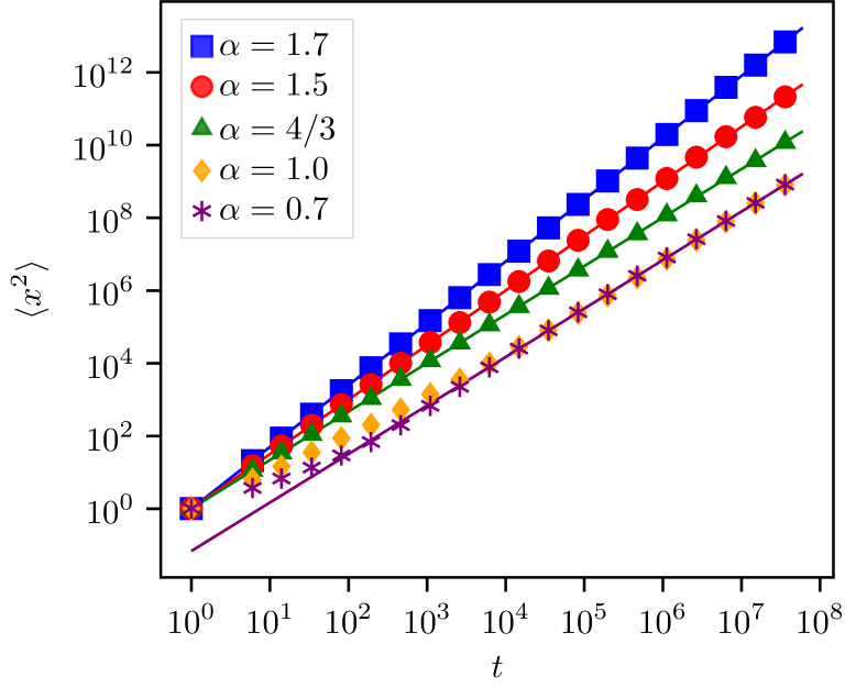
Figure 1: Mean-squared displacement $\langle x^{2}\rangle$ of FBM with mean-density interaction vs. time $t$ for interaction strength $A=1/40$ and several $\alpha$. The data are averages over 16 ensembles of 128 random walkers each. The resulting statistical errors are much smaller than the symbol size. The solid lines are power-law fits of the long-time behavior with $\langle x^{2}\rangle=c\,t^{\bar{\alpha}}$. They yield $\bar{\alpha}=\alpha$ for $\alpha\geq 4/3$ and $\bar{\alpha}=4/3$ for $\alpha<4/3$, for details see text.

In all cases, the mean-squared displacement follows a power-law time dependence $\langle x^{2}\rangle\sim t^{\bar{\alpha}}$ for sufficiently long times. Note that we need to distinguish the exponent $\alpha$ that parameterizes the fractional Gaussian noise, as defined in eq. (4), from the exponent $\bar{\alpha}$ that characterizes the mean-squared displacement of the interacting system.

A detailed analysis of the data in Fig. 1 reveals two different regimes. For $\alpha=1.7$, 1.5, and 4/3, the mean-squared displacement features power-law behavior over the entire time range. Fits with $\langle x^{2}\rangle\sim t^{\bar{\alpha}}$ where both $c$ and $\bar{\alpha}$ are fit parameters yield $\bar{\alpha}$ values very close to the corresponding FBM value $\alpha$. In fact, the data can be fitted with high quality (reduced $\chi^{2}$ values below unity) with $\bar{\alpha}$ fixed at $\bar{\alpha}=\alpha$. The solid lines in Fig. 1 for $\alpha=1.7$, 1.5, and 4/3 show these fits.

The data for $\alpha=0.7$ and 1.0, in contrast, show a more complex behavior. At short times, the mean-squared displacement $\langle x^{2}\rangle$ increases more slowly, as would be expected for (noninteracting) FBM with a lower $\alpha$. For longer times, $\langle x^{2}\rangle$ crosses over to a faster power-law behavior that can be fitted very well (reduced $\chi^{2}$ values below unity) with $\langle x^{2}\rangle\sim t^{\bar{\alpha}}$ with $\bar{\alpha}=4/3$ for both $\alpha=0.7$ and 1.0. The solid lines in Fig. 1 for $\alpha=0.7$ and 1 correspond to such fits for times larger than $10^{6}$. In fact, the mean-squared displacement curves for $\alpha=0.7$ and 1.0 are essentially indistinguishable for times beyond $10^{5}$. This suggests that the long-time behavior for these $\alpha$ values is dominated by interactions whereas the fractional Gaussian noise plays a subleading role.

Further evidence for a crossover between FBM-like behavior at short times and interaction-dominated behavior at long times can be found in Fig. 2 which shows the mean-squared displacement at $\alpha=0.7$ for several different interaction strengths $A$.

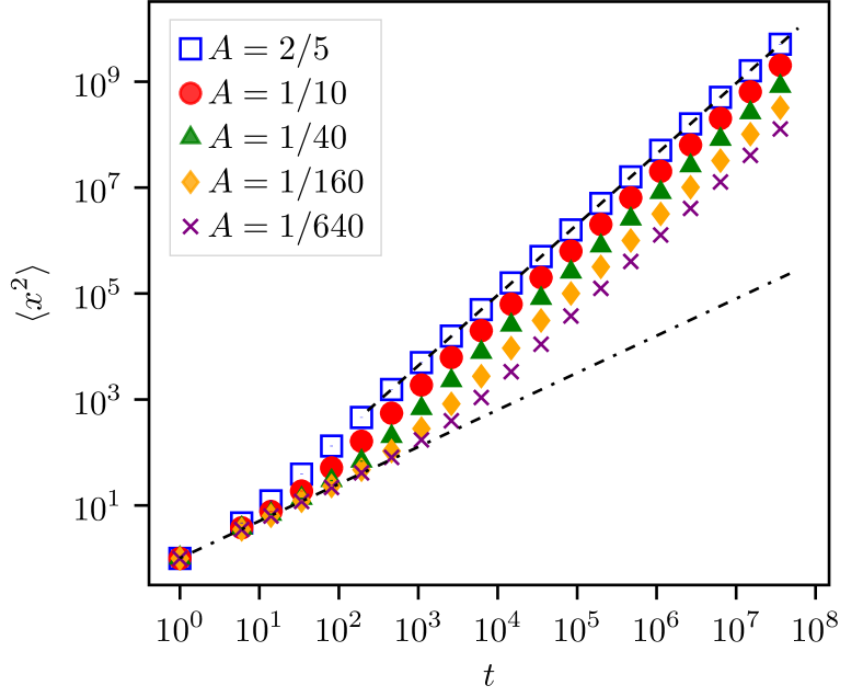
Figure 2: Mean-squared displacement $\langle x^{2}\rangle$ of FBM with mean-density interaction vs. time $t$ for $\alpha=0.7$ and serval values of the interaction strength $A$. The data are averages over 60 ensembles of 128 random walkers each. The resulting statistical errors are much smaller than the symbol size. The dashed line represents a fit of the long-time behavior for $A=2/5$ with $\langle x^{2}\rangle=c\,t^{4/3}$ whereas the dash-dotted line shows the FBM relation $\langle x^{2}\rangle=\sigma^{2}t^{0.7}$.

At the earliest times, the mean-squared displacements are independent of $A$ and follow the FBM relation $\langle x^{2}\rangle=\sigma^{2}t^{0.7}$. After a crossover time $t_{x}$, the behavior of the mean-squared displacement changes to $\langle x^{2}\rangle\sim t^{4/3}$ with an $A$-dependent prefactor. $t_{x}$ increases with decreasing interaction strength $A$.

This crossover behavior can be understood as follows. At short times, the integrated density $P_{\mathrm{int}}$ is small. The interaction terms (forces) (9) therefore do not yet play a role in the recursion relation (6), and the process behaves just like (non-interacting) FBM. As $P_{\mathrm{int}}$ increases with time, the interaction terms (9) also increase. At the crossover time $t_{x}$, they become comparable to the fractional Gaussian noise. The crossover time increases with decreasing interaction strength $A$ because, for smaller $A$, a larger integrated density $P_{\mathrm{int}}$ is required for the same generalized force $f$. Beyond the crossover time, the process is interaction dominated, as discussed above.

IV Scaling theory

In this section, we develop a scaling theory for FBM with mean-density interaction to explain the computer simulation results quantitatively. Consider an ensemble of $N$ random walkers starting at the origin $x=0$ at time $t=0$. The scaling theory is based on the assumption that, for sufficiently long times, the integrated distribution $P_{\mathrm{int}}(x,t)$ approaches a universal functional form characterized by a single length scale $b(t)$ that increases with time $t$. This can be expressed via the scaling ansatz

$$P_{\mathrm{int}}(x,t)=\frac{t}{b(t)}Y\left[\frac{x}{b(t)}\right]~.$$ (11)

The factor $t$ accounts for the fact that the space-integral over of the integrated density $P_{\mathrm{int}}(x,t)$ increases linearly with time. As a result, the scaling function $Y$ can be normalized to unity

$$\int_{-\infty}^{\infty}Y(y)dy=1~.$$ (12)

Using this scaling form, the force term in the FBM recursion (6) can be expressed as

$$f(x,t)=-A\frac{\partial}{\partial x}P_{\mathrm{int}}(x,t)=-\frac{At}{b^{2}(t)}Y^{\prime}\left[\frac{x}{b(t)}\right]~.$$ (13)

Here $Y^{\prime}$ denotes the derivative of the scaling function with respect to its argument. Let us further assume that the length scale $b(t)$ increases according to the power law

$$b(t)\sim t^{\delta}$$ (14)

with an unknown (positive) exponent $\delta$. Equation (13) then implies that the typical force varies with time as

$$f(x,t)\sim t^{1-2\delta}~.$$ (15)

If the force term dominates the motion of the particles (compared to the fractional Gaussian noise), the leading behavior of the displacement is simply given by a time integral over the force. The typical displacement is thus expected to behave as

$$x_{\mathrm{typ}}(t)\sim\int_{0}^{t}dt^{\prime}\,f_{\mathrm{typ}}(t^{\prime})\sim t^{2-2\delta}~.$$ (16)

For the theory to be self-consistent, the time dependence of $x_{\mathrm{typ}}$ needs to match the assumed time dependence of the length scale $b(t)$,

$$t^{\delta}\propto t^{2-2\delta}~,$$ (17)

yielding $\delta=2/3$. In the force-dominated regime, the mean-squared displacement is therefore expected to behave as

$$\langle x^{2}\rangle\sim b^{2}(t)\sim t^{4/3}~.$$ (18)

To further check the self-consistency of the scaling theory, let us discuss what happens if the length scale $b(t)$ increases faster than $t^{2/3}$, as is expected to happen if the motion is driven by fractional Gaussian noise with an anomalous diffusion exponent $\alpha>4/3$. In this case, the displacement contribution (16) resulting from integrating the forces would grow more slowly than $t^{2/3}$. This implies that the contribution of the forces to the displacement is subleading compared to the fractional Gaussian noise.

If we assume, on the other hand, that the length scale $b(t)$ increases more slowly than $t^{2/3}$, the hypothetical contribution of the forces to the displacement would increase faster than $t^{2/3}$, leading to a contradiction. The scaling theory therefore predicts that one-dimensional FBM with mean-density interaction in free space is dominated by the fractional Gaussian noise (and behaves like regular FBM) for $\alpha>4/3$ (i.e., $\gamma<2/3)$, whereas it is interaction-dominated for $\alpha<4/3$ (i.e., $\gamma>2/3$). This yields the following mean-squared displacement behaviors,

$$\langle x^{2}\rangle\sim\left\{\begin{array}[]{ll}t^{4/3}&\qquad\textrm{for }\alpha<4/3\\ t^{\alpha}=t^{2-\gamma}&\qquad\textrm{for }\alpha>4/3\end{array}\right.~.$$ (19)

These predictions agree with the Monte Carlo results of Sec. III.

V Results: Probability densities

In this section, we present the Monte Carlo results for the mean integrated density $P_{\mathrm{int}}$, defined in eqs. (5) and (9) as

$$P_{\mathrm{int}}(x,t_{n})=\frac{1}{N}\sum_{j=1}^{N}\sum_{m=1}^{n}\delta[x-x^{(j)}_{m}]~.$$ (20)

This not only provides additional insight into the behavior of FBM with mean-density interaction, but also allows us to test the assumptions underlying the scaling theory developed in Sec. IV. In addition, we also analyze the instantaneous (fixed time) probability density of the diffusing particles,

$$P(x,t_{n})=\frac{1}{N}\sum_{j=1}^{N}\delta[x-x^{(j)}_{n}]~.$$ (21)

In the application to serotonergic neurons, it represents the density of the active tips of the growing fibers.

For reference, we first consider the case of non-interacting FBM. The (instantaneous) probability density is given by eq. (2). It can be expressed in terms of the parameters of our discrete-time FBM version as

$$P(x,t_{n})=\frac{1}{\sqrt{2\pi\sigma^{2}t_{n}^{\alpha}}}\exp{\left(-\frac{x^{2}}{2\sigma^{2}t_{n}^{\alpha}}\right)}~.$$ (22)

The integrated density $P_{\mathrm{int}}(x,t_{n})$ is obtained by summing this Gaussian over time steps 1 to $n$. In the continuum limit, the summation can be replaced by an integration, yielding

$$P_{\mathrm{int}}(x,t_{n})=\frac{|x|^{2/\alpha-1}}{\alpha\pi^{1/2}(2\sigma^{2})^{1/\alpha}}\,\Gamma\left(\frac{1}{2}-\frac{1}{\alpha},\frac{x^{2}}{2\sigma^{2}t_{n}^{\alpha}}\right)~,$$ (23)

where $\Gamma$ is the incomplete Gamma function (for details, see the Appendix). This function has a maximum (with a cusp) at $x=0$ and a Gaussian tail (up to a power-law prefactor) for large $x$.

We now turn to our simulation results for the (instantaneous) probability density $P(x,t)$ and the time-integrated density $P_{\mathrm{int}}(x,t)$ for FBM with mean-density interaction. We have studied in detail two values of $\alpha$, one in the fractional-noise-dominated regime $\alpha>4/3$ and one in the interaction-dominated regime $\alpha<4/3$.

We start by discussing $\alpha=1.5$ in the noise-dominated regime. Figure 3(a) shows the integrated density for several different times.

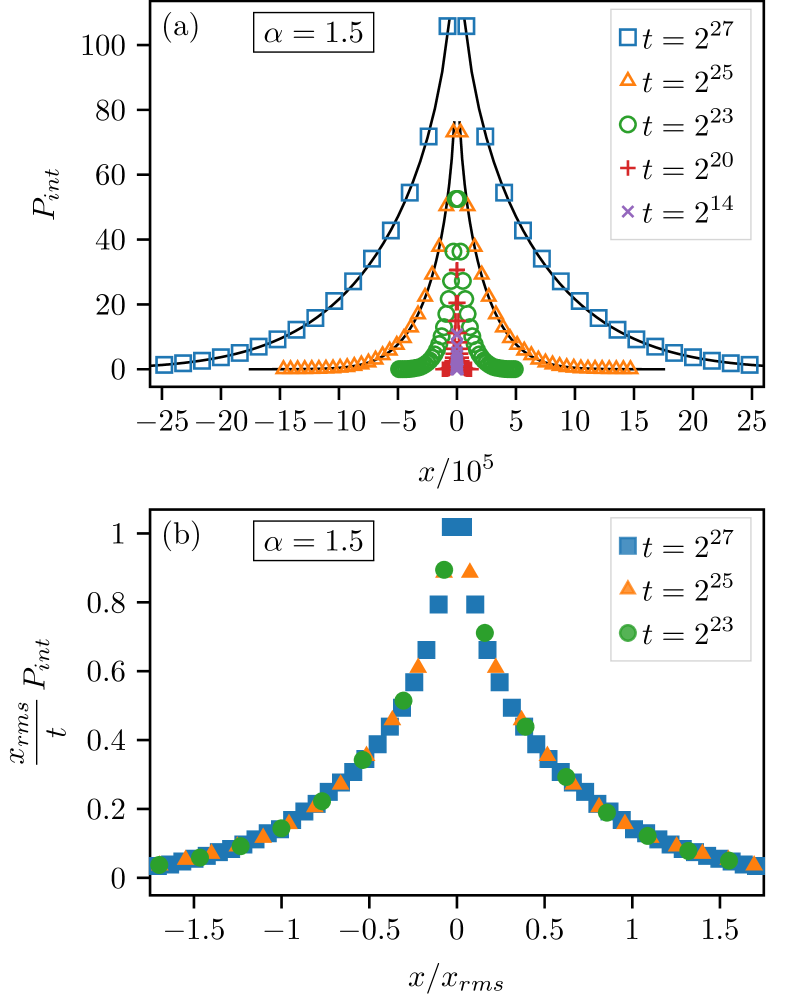
Figure 3: (a) Integrated density $P_{\mathrm{int}}(x,t)$ for $\alpha=1.5$, $A=1/40$, and several $t$. The data are averages over 120 ensembles of 64 random walkers each. To reduce the statistical noise in the figures, the histograms have been re-binned using 50 bins over the nonzero part of the histogram. The resulting statistical errors are much smaller than the symbol size. The solid lines shown for $t=2^{25}$ and $2^{27}$ correspond to the result (23) for noninteracting FBM. (b) Scaled integrated density $x_{\mathrm{rms}}P_{\mathrm{int}}(x,t)/t$ vs. $x/x_{\mathrm{rms}}$ with $x_{\mathrm{rms}}=\sqrt{\langle x^{2}(t)\rangle}$.

As expected, $P_{\mathrm{int}}$ broadens with time, and its normalization increases, reflecting the growth of the trajectories with time. Figure 3(a) also compares the simulation results for times $t=2^{25}$ and $2^{27}$ with the integrated density (23) of noninteracting FBM for the same $\alpha$. The agreement is nearly perfect and demonstrates that, for $\alpha=1.5$, the interaction does not affect the integrated density distribution at sufficiently long times. This agrees with the conclusion of the scaling theory of Sec. IV which predicts that for $\alpha>4/3$, the force terms in the recursion (6) become negligibly small compared to the fractional Gaussian noise for $t\to\infty$. Figure 3(b) shows that the integrated density fulfills the scaling form (11) with the root-mean-squared displacement $x_{\mathrm{rms}}(t)=\sqrt{\langle x^{2}(t)\rangle}$ playing the role of the length scale $b(t)$. This confirms the key assumption of the scaling theory.

In addition to the integrated density, we have also studied the (instantaneous) probability density $P(x,t)$. Simulation results for $\alpha=1.5$ are shown in Fig. 4(a).

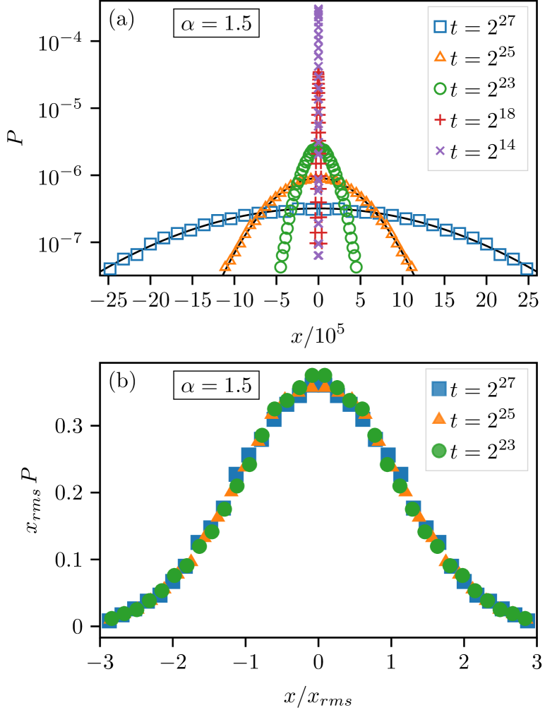
Figure 4: (a) (Instantaneous) probability density $P(x,t)$ for $\alpha=1.5$, $A=1/40$, and several $t$. The data are averages over 120 ensembles of 64 random walkers each. To reduce the statistical noise in the figures, the histograms have been re-binned using 50 bins over the nonzero part of the histogram. The resulting statistical errors are about the symbol size. The solid lines shown for $t=2^{25}$ and $2^{27}$ correspond to the Gaussian distribution (22) for noninteracting FBM. (b) Scaled probability density $x_{\mathrm{rms}}P(x,t)$ vs. $x/x_{\mathrm{rms}}$ with $x_{\mathrm{rms}}=\sqrt{\langle x^{2}(t)\rangle}$.

In agreement with the notion that the interactions become negligible for long times, $P(x,t)$ agrees with the Gaussian distribution (22) of (noninteracting) FBM. Figure 4(b) confirms that the probability density fulfills the scaling form

$$P(x,t)=\frac{1}{b(t)}Z\left[\frac{x}{b(t)}\right]$$ (24)

with $b(t)=x_{\mathrm{rms}}(t)=\sqrt{\langle x^{2}(t)\rangle}$ and $Z$ being a dimensionless scaling function. Of course, for noninteracting FBM, this follows directly from eq. (22).

After having discussed the fractional-noise-dominated regime $\alpha>4/3$, we now consider the interaction-dominated regime $\alpha<4/3$. This regime is arguably more interesting, because we expect the behavior of our process to differ qualitatively from that of noninteracting FBM. We have performed extensive simulations for $\alpha=0.7$ and 1.0 in the interaction-dominated regime. In the following, we discuss the case $\alpha=1.0$ as an example.

Figure 5(a) shows the time-integrated density $P_{\mathrm{int}}(x,t)$ for $\alpha=1.0$ and several values of the time $t$.

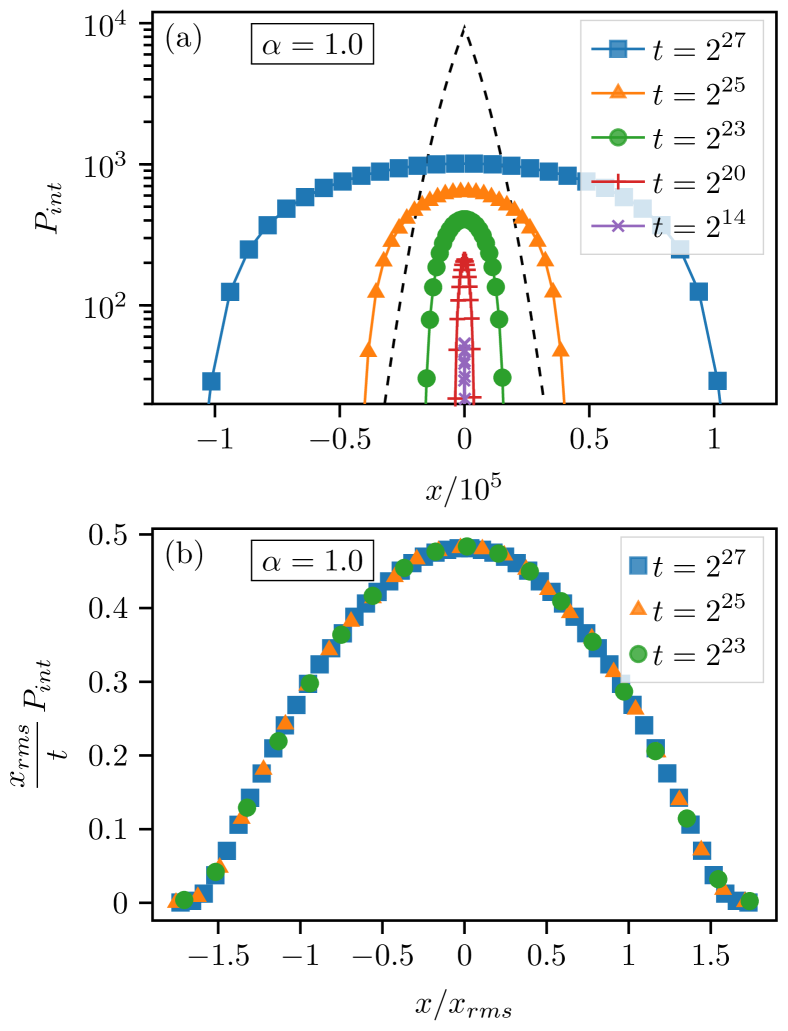
Figure 5: (a) Integrated density $P_{\mathrm{int}}(x,t)$ for $\alpha=1.0$, $A=1/40$, and several $t$. The data are averages over 120 ensembles of 64 random walkers each. To reduce the statistical noise in the figures, the histograms have been re-binned using 30 bins over the nonzero part of the histogram. The resulting statistical errors are much smaller than the symbol size. For comparison, the dashed line shows the result (23) for noninteracting FBM at time $t=2^{27}$. (b) Scaled integrated density $x_{\mathrm{rms}}P_{\mathrm{int}}(x,t)/t$ vs. $x/x_{\mathrm{rms}}$ with $x_{\mathrm{rms}}=\sqrt{\langle x^{2}(t)\rangle}$.

$P_{\mathrm{int}}$ broadens with time, and its normalization increases, as expected. The figure also presents (as a dashed line) the integrated density (23) of noninteracting FBM for the same $\alpha=1$ at time $t=2^{27}$. The data clearly show that the interacting integrated density is much broader than that of noninteracting FBM, and it has a different shape (in particular, no cusp at $x=0$). This agrees with the notion that, for $\alpha<4/3$, the interactions dominate the time evolution and lead to a more rapid expansion of the particle “cloud” than the fractional Gaussian noise would. Nonetheless, the integrated density fulfills the scaling form (11) with $b(t)=x_{\mathrm{rms}}(t)=\sqrt{\langle x^{2}(t)\rangle}$, as is demonstrated in Fig. 5(b). This confirms that the key assumption of the scaling theory holds not just in the fractional-noise-dominated regime but also in the interaction-dominated regime.

Simulation results for the (instantaneous) probability density $P(x,t)$ for $\alpha=1.0$ are shown in Fig. 6(a).

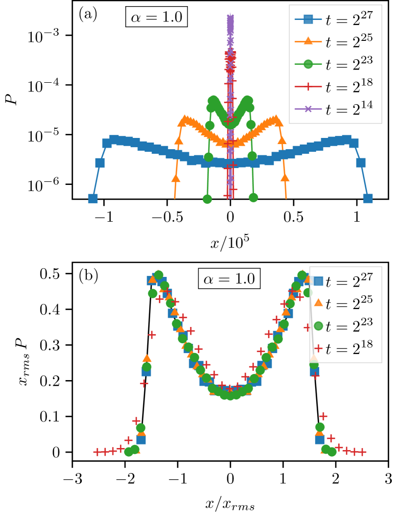
Figure 6: (a) (Instantaneous) probability density $P(x,t)$ for $\alpha=1.0$, $A=1/40$, and several $t$. The data are averages over 120 ensembles of 64 random walkers each. To reduce the statistical noise in the figures, the histograms have been re-binned using 40 bins over the nonzero part of the histogram. The resulting statistical errors are about the symbol size. (b) Scaled probability density $x_{\mathrm{rms}}P(x,t)$ vs. $x/x_{\mathrm{rms}}$ with $x_{\mathrm{rms}}=\sqrt{\langle x^{2}(t)\rangle}$.

The figure demonstrates that the probability density in the interaction-dominated regime differs significantly from that of FBM and is highly non-Gaussian. Interestingly, the maximum of $P(x,t)$ is not at the center $x=0$. Instead, there are two symmetric maxima after which $P(x,t)$ rapidly drops to zero. This can be understood as follows. In the interaction-dominated regime, the force terms in the recursion (6) push the particles strongly away from the center region where the integrated density (i.e., the density of the entire ensemble of trajectories) accumulated during previous time steps. At any given time, the “active” particles (i.e., the tips of the trajectories) are therefore concentrated near the boundary of the integrated density. For example, Fig. 5(a) shows that the integrated density at $t=2^{27}$ roughly extends to $x=\pm 10^{5}$. Correspondingly, the maxima of the instantaneous probability density in Fig. 6(a) for $t=2^{27}$ are at positions $x\approx\pm 10^{5}$.

Despite its highly non-Gaussian form, the probability density in the interaction-dominated regime fulfills the scaling form (24) with $b(t)=x_{\mathrm{rms}}(t)=\sqrt{\langle x^{2}(t)\rangle}$, as can be seen in Fig. 6(b). The small deviations from perfect scaling collapse for the shortest time in the figure can be attributed to finite-time effects. Specifically, the force terms do not completely dominate at $t=2^{18}$, and the fractional Gaussian noise produces the small tails at large $|x|$.

We note that similar bimodal probability densities are observed, for different physical reasons, in Levy walks, certain heterogeneous diffusion processes, fractional wave equations, and the end-to-end distance of semi-flexible polymers.

VI Generalizations

So far, we have considered motion in one space dimension under the influence of a force that is proportional to the gradient of the integrated density. It is interesting to ask how the system behaves in higher dimensions and for other functional forms of the density-dependent force. The scaling theory of Sec. IV is easily generalized to $d$ space dimensions and forces that behave as the $\lambda$-th power of the gradient of $P_{\mathrm{int}}(\mathbf{x},t_{n})$.

In $d$ dimensions, the scaling form (11) of the integrated mean density generalizes to

$$P_{\mathrm{int}}(\mathbf{x},t)=\frac{t}{b^{d}(t)}Y\left[\frac{\mathbf{x}}{b(t)}\right]~.$$ (25)

If we again assume that the length scale $b(t)$ increases as $t^{\delta}$ with unknown $\delta$, the force term behaves as

$$|\mathbf{f}(\mathbf{x},t)|=\left|A\frac{\partial}{\partial\mathbf{x}}P_{\mathrm{int}}(\mathbf{x},t)\right|^{\lambda}\sim t^{\lambda-(d+1)\delta\lambda}~.$$ (26)

In the force-dominated regime, the typical displacement is obtained by integrating this force over time. It is thus expected to behave as $x_{\mathrm{typ}}\sim t^{1+\lambda-(d+1)\delta\lambda}$. Self-consistency with the assumption $b(t)\sim t^{\delta}$ requires $1+\lambda-(d+1)\delta\lambda=\delta$. Solving for the value of $\delta$ yields

$$\delta=\frac{1+\lambda}{1+(d+1)\lambda}~.$$ (27)

For $d=\lambda=1$, we recover the result of Sec.  IV, $\delta=2/3$.

Repeating the arguments at the end of Sec.  IV, we conclude that the motion of FBM with mean-density interaction will be interaction dominated if the FBM anomalous diffusion exponent $\alpha$ is smaller than $2\delta$. In this case the mean-squared displacement is expected to behave as $\langle\mathbf{x}^{2}\rangle\sim t^{2\delta}$. If on the other hand, $\alpha>2\delta$, the motion will be dominated by the fractional Gaussian noise leading to $\langle\mathbf{x}^{2}\rangle\sim t^{\alpha}$. Equation (27) shows that $\delta$ decreases with increasing space dimensionality $d$. This implies that the marginal value of $\alpha$, below which the interactions dominate over the noise, decreases with increasing $d$. The result that the interaction effects are strongest in one dimension and decrease with increasing $d$ is perhaps not unexpected as crowding is more easily achieved in lower dimensions.

Computer simulations of FBM in higher space dimensions require a significantly larger numerical effort. For this reason, a numerical test of the generalized scaling theory is relegated to future work.

VII Conclusions

In this paper, we have introduced FBM with mean-density interaction, a process in which each particle of an ensemble evolves under the influence of both fractional Gaussian noise and a force proportional to the gradient of the time-integrated density of the entire ensemble. This work was motivated by the recent application of (reflected) FBM to the growth of serotonergic fibers in vertebrate brains [29, 30, 31]. However, we believe our model to be applicable to a much broader class of anomalous diffusion processes in which the particles interact with a (coarse-grained) density of the resulting trajectories.

Employing large-scale computer simulations as well as a one-parameter scaling theory, we have found that the behavior of one-dimensional, unbounded FBM with mean-density interaction falls in one of two regimes, depending on the value of the exponent $\alpha$ characterizing the fractional Gaussian noise. For $\alpha>4/3$, the long-time behavior is governed by the fractional Gaussian noise, and the force terms become negligibly small. Consequently, in this regime, the mean-squared displacement and the probability density agree with the corresponding quantities of noninteracting FBM for sufficiently long times. For $\alpha<4/3$, in contrast, the long-time behavior of the model is dominated by the interactions, and the fractional Gaussian noise only makes subleading contributions. As a result, the mean-squared displacement grows like $t^{4/3}$ for all $\alpha\leq 4/3$ and the probability density becomes highly non-Gaussian.

Our work suggests many interesting extensions that may stimulate further research. These include the questions of higher space dimensions and nonlinear forces that we have already touched upon in Sec.  VI. It is also interesting to study what happens in applications in which the particles are attracted rather than repulsed by regions of high (integrated) density. Moreover, we expect a nontrivial interplay between the mean-density interaction and reflecting walls that confine the process to some finite or semi-finite region of space. In the current model, motivated by the growth of serotonergic fibers in the brain, the particles interact with the density of the entire trajectory ensemble, accumulated since the starting time. In addition, one can ask what changes if the interaction effect decays over time. These and other questions remain tasks for the future.

Appendix A Integrated density of FBM

In this Appendix, we sketch the derivation of the expression (23) for the integrated density of (non-interacting) FBM. Equations (20) and (21) imply that the integrated density simply is a sum over the (instantaneous) probability densities,

$$P_{\mathrm{int}}(x,t_{n})=\sum_{m=1}^{n}P(x,t_{m})~.$$ (28)

As we are interested in the continuum limit $t\gg\epsilon=1$ (or $n\gg 1$), the sum can be replaced by an integral which reads

$$P_{\mathrm{int}}(x,t) = \int_{0}^{t}d\tau P(x,\tau)$$ (29)

$$= \int_{0}^{t}d\tau\frac{1}{\sqrt{2\pi\sigma^{2}\tau^{\alpha}}}\exp{\left(-\frac{x^{2}}{2\sigma^{2}\tau^{\alpha}}\right)}$$

Substituting $z=x^{2}/(2\sigma^{2}\tau^{\alpha})$ leads to

$$P_{\mathrm{int}}(x,t)=\frac{|x|^{2/\alpha-1}}{\alpha\pi^{1/2}(2\sigma^{2})^{1/\alpha}}\int_{x^{2}/(2\sigma^{2}t^{\alpha})}^{\infty}dz\,z^{-1/\alpha-1/2}e^{-z}~.$$ (30)

The integral over $z$ yields the incomplete Gamma function, which concludes the derivation of eq. (23). It is worth emphasizing that the expression (23) fulfills the scaling form (11) with $b(t)=x_{\mathrm{rms}}(t)=\sigma t^{\alpha/2}$. This can be seen explicitly by rewriting (23) as

$$P_{\mathrm{int}}(x,t) = \frac{t}{\sigma t^{\alpha/2}}\,Y\left(\frac{x}{\sigma t^{\alpha/2}}\right)$$ (31)

$$Y(y) = \frac{1}{\alpha\pi^{1/2}2^{1/\alpha}}\,|y|^{2/\alpha-1}\Gamma\left(\frac{1}{2}-\frac{1}{\alpha},\frac{y^{2}}{2}\right)~.~$$ (32)

References

- Brown [1828] R. Brown, A brief account of microscopical observations made in the months of June, July and August 1827, on the particles contained in the pollen of plants; and on the general existence of active molecules in organic and inorganic bodies, Phil. Mag. 4, 161 (1828).
- Einstein [1956] A. Einstein, Investigations on the Theory of the Brownian Movement (Dover, New York, 1956).
- von Smoluchowski [1918] M. von Smoluchowski, Versuch einer mathematischen Theorie der Koagulationskinetik kolloider Lösungen, Z. Phys. Chem. 92U, 129 (1918).
- Langevin [1908] P. Langevin, Sur la théorie du mouvement brownien, C. R. Acad. Sci. Paris 146, 530 (1908).
- Hughes [1995] B. Hughes, Random Walks and Random Environments, Volume 1: Random Walks (Oxford University Press, Oxford, 1995).
- Metzler and Klafter [2000] R. Metzler and J. Klafter, The random walk’s guide to anomalous diffusion: a fractional dynamics approach, Physics Reports 339, 1 (2000).
- Höfling and Franosch [2013] F. Höfling and T. Franosch, Anomalous transport in the crowded world of biological cells, Rep. Progr. Phys. 76, 046602 (2013).
- Bressloff and Newby [2013] P. C. Bressloff and J. M. Newby, Stochastic models of intracellular transport, Rev. Mod. Phys. 85, 135 (2013).
- Metzler et al. [2014] R. Metzler, J.-H. Jeon, A. G. Cherstvy, and E. Barkai, Anomalous diffusion models and their properties: non-stationarity, non-ergodicity, and ageing at the centenary of single particle tracking, Phys. Chem. Chem. Phys. 16, 24128 (2014).
- Meroz and Sokolov [2015] Y. Meroz and I. M. Sokolov, A toolbox for determining subdiffusive mechanisms, Physics Reports 573, 1 (2015).
- Metzler et al. [2016] R. Metzler, J.-H. Jeon, and A. Cherstvy, Non-Brownian diffusion in lipid membranes: Experiments and simulations, Biochimica et Biophysica Acta 1858, 2451 (2016).
- Nørregaard et al. [2017] K. Nørregaard, R. Metzler, C. M. Ritter, K. Berg-Sørensen, and L. B. Oddershede, Manipulation and motion of organelles and single molecules in living cells, Chemical Reviews 117, 4342 (2017).
- Kolmogorov [1940] A. N. Kolmogorov, Wienersche Spiralen und einige andere interessante Kurven im Hilbertschen raum, C. R. (Doklady) Acad. Sci. URSS (N.S.) 26, 115 (1940).
- Mandelbrot and Ness [1968] B. B. Mandelbrot and J. W. V. Ness, Fractional brownian motions, fractional noises and applications, SIAM Review 10, 422 (1968).
- Szymanski and Weiss [2009] J. Szymanski and M. Weiss, Elucidating the origin of anomalous diffusion in crowded fluids, Phys. Rev. Lett. 103, 038102 (2009).
- Magdziarz et al. [2009] M. Magdziarz, A. Weron, K. Burnecki, and J. Klafter, Fractional Brownian motion versus the continuous-time random walk: A simple test for subdiffusive dynamics, Phys. Rev. Lett. 103, 180602 (2009).
- Weber et al. [2010] S. C. Weber, A. J. Spakowitz, and J. A. Theriot, Bacterial chromosomal loci move subdiffusively through a viscoelastic cytoplasm, Phys. Rev. Lett. 104, 238102 (2010).
- Jeon et al. [2011] J.-H. Jeon, V. Tejedor, S. Burov, E. Barkai, C. Selhuber-Unkel, K. Berg-Sørensen, L. Oddershede, and R. Metzler, In vivo anomalous diffusion and weak ergodicity breaking of lipid granules, Phys. Rev. Lett. 106, 048103 (2011).
- Jeon et al. [2012] J.-H. Jeon, H. M.-S. Monne, M. Javanainen, and R. Metzler, Anomalous diffusion of phospholipids and cholesterols in a lipid bilayer and its origins, Phys. Rev. Lett. 109, 188103 (2012).
- Tabei et al. [2013] S. M. A. Tabei, S. Burov, H. Y. Kim, A. Kuznetsov, T. Huynh, J. Jureller, L. H. Philipson, A. R. Dinner, and N. F. Scherer, Intracellular transport of insulin granules is a subordinated random walk, Proc. Nat. Acad. Sci. 110, 4911 (2013).
- Chakravarti and Sebastian [1997] N. Chakravarti and K. Sebastian, Fractional Brownian motion models for polymers, Chem. Phys. Lett. 267, 9 (1997).
- Panja [2010] D. Panja, Generalized Langevin equation formulation for anomalous polymer dynamics, J. Stat. Mech. 2010, L02001 (2010).
- Mikosch et al. [2002] T. Mikosch, S. Resnick, H. Rootzen, and A. Stegeman, Is network traffic appriximated by stable Levy motion or fractional Brownian motion?, Ann. Appl. Probab. 12, 23 (2002).
- Comte and Renault [1998] F. Comte and E. Renault, Long memory in continuous-time stochastic volatility models, Math. Financ. 8, 291 (1998).
- Rostek and Schöbel [2013] S. Rostek and R. Schöbel, A note on the use of fractional Brownian motion for financial modeling, Econom. Model. 30, 30 (2013).
- Wada and Vojta [2018] A. H. O. Wada and T. Vojta, Fractional Brownian motion with a reflecting wall, Phys. Rev. E 97, 020102 (2018).
- Guggenberger et al. [2019] T. Guggenberger, G. Pagnini, T. Vojta, and R. Metzler, Fractional Brownian motion in a finite interval: correlations effect depletion or accretion zones of particles near boundaries, New J. Phys. 21, 022002 (2019).
- Vojta et al. [2020] T. Vojta, S. Halladay, S. Skinner, S. Janušonis, T. Guggenberger, and R. Metzler, Reflected fractional Brownian motion in one and higher dimensions, Phys. Rev. E 102, 032108 (2020).
- Janušonis and Detering [2019] S. Janušonis and N. Detering, A stochastic approach to serotonergic fibers in mental disorders, Biochimie 161, 15 (2019).
- Janušonis et al. [2020] S. Janušonis, N. Detering, R. Metzler, and T. Vojta, Serotonergic axons as fractional Brownian motion paths: Insights into the self-organization of regional densities, Front. Comp. Neuroscience 14, 56 (2020).
- Janušonis et al. [2023] S. Janušonis, J. H. Haiman, R. Metzler, and T. Vojta, Predicting the distribution of serotonergic axons: a supercomputing simulation of reflected fractional Brownian motion in a 3d-mouse brain model, Front. Comp Neurosci. 17, 1189853 (2023).
- Daubert et al. [2010] E. A. Daubert, D. S. Heffron, J. W. Mandell, and B. G. Condron, Serotonergic dystrophy induced by excess serotonin, Mol Cell Neurosci. 44, 297 (2010).
- Migliarini et al. [2013] S. Migliarini, G. Pacini, B. Pelosi, G. Lunardi, and M. Pasqualetti, Lack of brain serotonin affects postnatal development and serotonergic neuronal circuitry formation, Mol Psychiatry 18, 1106 (2013).
- Vicenzi et al. [2021] S. Vicenzi, L. Foa, and R. J. Gasperini, Serotonin functions as a bidirectional guidance molecule regulating growth cone motility, Cell Mol Life Sci. 78, 2247 (2021).
- Chen et al. [2017] W. V. Chen, C. L. Nwakeze, C. A. Denny, S. O’Keeffe, M. A. Rieger, G. Mountoufaris, A. Kirner, J. D. Dougherty, R. Hen, Q. Wu, and T. Maniatis, Pcdhac2 is required for axonal tiling and assembly of serotonergic circuitries in mice, Science 356, 406 (2017).
- Nazzi et al. [2019] S. Nazzi, G. Maddaloni, M. Pratelli, and M. Pasqualetti, Fluoxetine induces morphological rearrangements of serotonergic fibers in the hippocampus, ACS Chemical Neuroscience 10, 3218 (2019), pMID: 31243951.
- Nazzi et al. [2024] S. Nazzi, M. Picchi, S. Migliarini, G. Maddaloni, N. Barsotti, and M. Pasqualetti, Reversible morphological remodeling of prefrontal and hippocampal serotonergic fibers by fluoxetine, ACS Chemical Neuroscience 15, 1702 (2024), pMID: 38433715.
- Qian [2003] H. Qian, Fractional brownian motion and fractional gaussian noise, in Processes with Long-Range Correlations: Theory and Applications, edited by G. Rangarajan and M. Ding (Springer, Berlin, Heidelberg, 2003) pp. 22–33.
- Makse et al. [1996] H. A. Makse, S. Havlin, M. Schwartz, and H. E. Stanley, Method for generating long-range correlations for large systems, Phys. Rev. E 53, 5445 (1996).
- L’Ecuyer [1999] P. L’Ecuyer, Tables of maximally equidistributed combined lfsr generators, Math. Comput. 68, 261 (1999).
- Marsaglia [2005] G. Marsaglia, Double precision RNGs, Posted to sci.math.num-analysis (2005), http://sci.tech-archive.net/Archive/sci.math.num-analysis/2005-11/msg00352.html.
- Note [1] If the functions in the definition (5) of are not smoothed, however, the histogram of the mean integrated density develops an unphysical oscillatory instability.