QuMATL: Query-based Multi-annotator Tendency Learning

Abstract.

Different annotators often assign different labels to the same sample due to backgrounds or preferences, and such labeling patterns are referred to as “tendency”. In multi-annotator scenarios, we introduce a novel task called Multi-annotator Tendency Learning (MATL), which aims to capture each annotator’s tendency. Unlike traditional tasks that prioritize consensus-oriented learning, which averages out annotator differences and leads to tendency information loss, MATL emphasizes learning each annotator’s tendency, better preserves tendency information. To this end, we propose an efficient baseline method, Query-based Multi-annotator Tendency Learning (QuMATL), which uses lightweight query to represent each annotator for tendency modeling. It saves the costs of building separate conventional models for each annotator, leverages shared learnable queries to capture inter-annotator correlations as an additional hidden supervisory signal to enhance modeling performance. Meanwhile, we provide a new metric, Difference of Inter-annotator Consistency (DIC), to evaluate how effectively models preserve annotators’ tendency information. Additionally, we contribute two large-scale datasets, STREET and AMER, providing averages of 4,300 and 3,118 per-annotator labels, respectively. Extensive experiments verified the effectiveness of our QuMATL.

1. Introduction

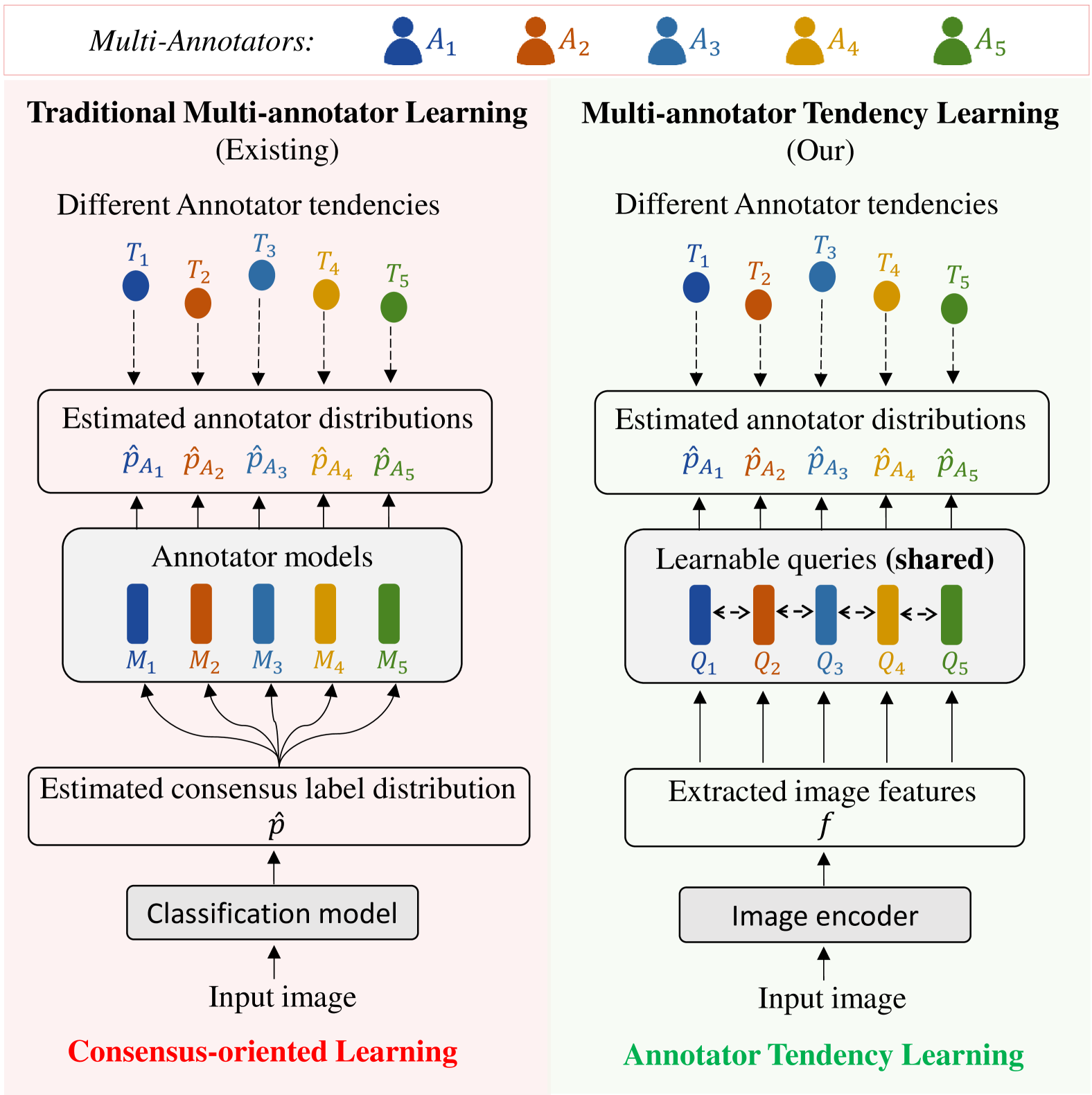
Figure 1. Task and model comparisons. We take five different annotators as an example. They give different labels to the same image due to preferences, we define such labeling patterns as tendency, corresponding to circles at different positions reflected dataset labels. The existing task in left focus on a consensus-oriented learning, uses multi-annotator supervision to indirectly train for a single consensus label prediction, easily tends to average out annotator differences leading to tendency information loss. Our introduced new task MATL focuses on learning each annotator’s tendency by only building a dedicated annotator model, which can better preserve tendency information. Compared to existing methods, our proposed QuMATL uses lightweight query to represent each annotator for tendency modeling and save costs of building separate conventional models for each annotator, leverages shared learnable queries to capture inter-annotator correlations as an additional hidden supervisory signal to enhance modeling performance.

In real-world multi-annotation scenarios, such as medical image analysis (Liao et al., 2024), sentiment analysis (Lian et al., 2023), and visual perception (Zhang et al., 2023c), different annotators often provide different labels to the same sample (Raykar et al., 2010) due to different personal backgrounds, subjective interpretations, and preferences. We refer to such labeling patterns exhibited by each annotator as tendency, and we introduce a new task called Multi-annotator Tendency Learning (MATL), which aims to capture each annotator’s tendency.

Let us suppose we have five annotators $A_{i},i\in\{1,\cdots,5\}$ for example, as shown in Figure 1, and use circles at different positions to represent the varying tendency $T_{i}$ of annotators reflected in the multi-annotator dataset labels. The left part represents the traditional multi-annotator learning tasks, which typically implement consensus-oriented learning. For example, it often builds a classification model that outputs a unique consensus label distribution prediction $\hat{p}$ for an input image and builds annotator models that capture different tendency of each annotator to predict each annotator’s label distribution$\hat{p}_{A_{i}}$ the input image. These models are trained with a dataset with multi-annotator labels. This way, a single model is trained through the labels from multiple annotators. This consensus-oriented learning often has an impact on the effects of the annotator tendency capturing process, such as reducing different annotators’ nuanced judgments on individual samples to simplified prediction-level biases, which easily causes tendency information loss during annotator modeling, i.e., the learned annotator models reduced differences among annotators’ tendencies.

In contrast, the right part illustrates our introduced MATL task, which focuses on annotator tendency learning. It emphasizes building models for different annotators to learn their tendencies, and then attempts to validate that these trained models with more tendency information effectively help implement specific tasks better. To this end, we proposed a query-based multi-annotator tendency learning (QuMATL) method. It assumes that differences between annotators are attributed to what observers focus on. Our method leverages learnable queries (${Q}_{i}$) of query transformer (Q-Former) (Li et al., 2023) to model different annotators’ tendencies, uses cross-attention module to interact with image features $f$ extracted by image encoder from the input image to capture different annotators’ nuanced judgments to maximize preservation of tendency information, and then predicts the annotator’s label distributions for an input image ($\hat{p}_{A_{i}}$) supervised by multi-annotator dataset labels for training. This way, our learned annotator models better preserve the differences among annotators’ tendencies, can gain more information about the annotator’s tendency.

Compared to the existing methods, which typically build separate annotator models (shown in the left figure) for each annotator without considering inter-annotator correlations, which makes individual annotator modeling only rely on annotator labels for learning, our method QuMATL shared all specified annotators’ queries (i.e., ${Q}_{i}$ in the right figure) in the Q-Former’s self-attention module. This allows the model to capture inter-annotator correlations, providing an additional hidden supervisory signal from inter-annotator consistency to enhance modeling performance. Here, inter-annotator consistency reflects the agreement levels among annotators on given samples. Additionally, lightweight representing each annotator by query greatly reduces the cost of building separate conventional models for each annotator.

To evaluate how effectively the trained model preserves annotator tendency information, we provide a novel metric, the difference of inter-annotator consistency (DIC), which quantifies how inter-annotator correlations differ between ground-truths and predictions. To maximize the preservation of annotator tendency information, their correlation coefficients should be close, with smaller differences indicating that the model captures correlations and reflecting that the model well preserves the inherent patterns of disagreement among annotators.

Furthermore, we constructed two new large-scale datasets: STREET (city impression evaluation) and AMER (video emotion recognition), each providing substantial consecutive labels per annotator ID. In contrast, although crowdsourcing platforms have numerous annotators, only a small subset of samples are annotated consecutively with consistent annotator IDs. Our datasets offer valuable open-source resources to the community and further researchers. It is worth noting that AMER is the first multi-annotator multimodal dataset in this field. Our work makes the following contributions:

• A new multi-annotator tendency learning task: We introduce a new MATL task that focuses on learning each annotator’s tendency, better preserves tendency information. In contrast, existing tasks focus on consensus-oriented learning, learning a consensus label prediction via multi-annotator supervision, which easily averages out annotator differences and leads to tendency information loss.

• An efficient query-based baseline method for new task: We propose a model QuMATL that uses lightweight queries to represent each annotator for tendency modeling and save costs of building separate conventional models for each annotator, leverages shared learnable queries to capture inter-annotator correlations as an additional hidden supervisory signal to enhance modeling performance.

• Two new large-scale datasets, a new metric: We contribute two new datasets: STREET and AMER, providing averages of 4,300 and 3,118 per-annotator labels. We provide a new DIC metric to evaluate how effectively models preserve annotators’ tendency information.

Table 1. Dataset comparison. Compared to existing multi-annotator datasets, our dataset contains a greater number of samples annotated by each annotator, which helps promote annotator tendency learning. Meanwhile, AMER is the first multimodal multi-annotator dataset.

Dataset	Dataset description	Modality	# samples per annotator
QUBIQ-kidney (Menze et al., 2020)	kidney image	image	24
QUBIQ-tumor (Menze et al., 2020)	brain tumor image	image	32
QUBIQ-growth (Menze et al., 2020)	brain growth image	image	39
QUBIQ-prostate (Menze et al., 2020)	prostate image	image	55
CIFAR-10H (Peterson et al., 2019b)	object recognition	image	200
MUSIC (Rodrigues et al., 2013a)	music genre classification	audio	2$\sim$368
MURA (Rajpurkar et al., 2017)	radiographic image	image	556
RIGA (Almazroa et al., 2017)	retinal cup and disc segmentation	image	750
LIDC-IDRI (Armato III et al., 2011)	lung nodule image	image	1,018
STREET (Ours)	city impression evaluation	image	4,300
AMER (Ours)	video emotion recognition	audio, video, text	970$\sim$5,202

2. Related work

2.1. Multi-annotator Tendency Learning Task

To the best of our knowledge, the multi-annotator tendency learning task has not yet been investigated. Traditional multi-annotator learning tasks focus on estimating consensus or ground-truth labels from multiple noisy annotations. These include early probabilistic models (Dawid and Skene, 1979), EM algorithms (Whitehill et al., 2009), Gaussian models (Rodrigues et al., 2014), and biased estimation (Welinder et al., 2010). Tanno et al. (Tanno et al., 2019a) proposed modeling annotator confusion matrices as learnable parameters in neural networks. Cao et al. (Cao et al., 2019) introduced max-MIG to learn from multiple annotators. NEAL (Chen et al., 2023) employs neural expectation-maximization to jointly learn annotator expertise and true labels. Later methods used probabilistic frameworks to aggregate multiple annotations into a consensus or ground-truth label by confusion matrix (Tanno et al., 2019b), agreement distribution (Wang et al., 2023), and Gaussian distributions (Liao et al., 2024). This consensus-oriented learning often easily averages out annotator differences and leads to tendency information loss. In contrast, our introduced MATL task focuses on learning each annotator’s tendency, better preserving tendency information.

2.2. Annotator Tendency Learning Framework

Previous studies typically construct independent models for each annotator to learn their specific behavioral patterns (Hashmi et al., 2023), or build separate distributions based on input features to fit each annotator (Liao et al., 2024), or use individual confusion matrices to approximate each annotator’s tendencies (Zhang et al., 2023c). Recent research associates annotator influences with model outcomes. TAX (Cheng et al., 2023) explains pixel-level assignment decisions for semantic segmentation by associating learned convolutional kernels with a prototype library representing annotator tendencies. MAGI (Zhang et al., 2023a) leverages multiple annotators’ explanations addressing challenges of noisy annotations and missing annotator correspondences. Schaekermann et al. (Schaekermann et al., 2019) revealed how factors like expert background and data quality contribute to annotation disagreements. These approaches build separate conventional models for each annotator without considering inter-annotator correlations, which makes individual annotator modeling only rely on annotator labels for learning. In contrast, our method QuMATL uses lightweight queries to represent each annotator for tendency modeling and save the costs of building separate conventional models for each annotator. It also leverages shared learnable queries to capture inter-annotator correlations as an additional hidden supervisory signal to enhance modeling performance.

2.3. Multi-annotator Datasets

Most existing multi-annotator datasets often have only a small subset of samples with consecutive annotations from consistent annotator IDs. CIFAR-10H (Peterson et al., 2019a), based on the CIFAR-10 (Krizhevsky, 2009) dataset, includes 10,000 test samples labeled by 2,571 annotators, but each annotator ID has on average only about 200 consecutive labels. LabelMe (Rodrigues and Pereira, 2018) includes an average of approximately 42.4 consecutive labels per annotator ID. Audio dataset Music (Rodrigues et al., 2013b) contains an average of about 46.1 consecutive labels. The medical datasets are commonly used in multi-annotator studies, consecutive annotator labels are even sparser. QUBIQ (Ji et al., 2021), a dataset for quantifying uncertainty in biomedical image segmentation, includes four distinct segmentation datasets with an average of only 40 samples, and even then, annotator IDs have only around 8 consecutive labeled samples each. More consecutive individual annotator labels facilitate MATL, we contribute two large-scale datasets: STREET and AMER, averaging 4,300 and 3,118 consecutive labels per annotator ID, respectively. These datasets contribute significant open-source resources that we believe will benefit the research community.

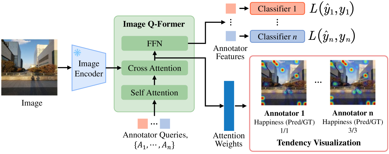
Figure 2. QuMATL architecture for image-specific pipeline. A frozen pre-trained image encoder extracts features, which interact with annotator-specific learnable queries in the Image Q-Former through cross-attention, producing annotator-specific features for classification. Different annotators’ cross-attention weights represent different annotator tendencies and provide visualization for analysis.

3. Dataset Construction

We contribute two new large-scale datasets: STREET (city impression assessment) and AMER (multi-modal emotion recognition) for our introduced MATL task. Table 1 compares the current multi-annotator datasets. We observe that in existing datasets, the number of samples annotated by each annotator is relatively small, and there is a lack of multi-annotator multimodal datasets. For example, in the RIGA dataset (Almazroa et al., 2017), each annotator labels 750 samples, while in the CIFAR-10H dataset (Peterson et al., 2019b), each annotator labels 200 samples.

(1) STREET is an urban perception dataset with multi-annotators, which contains $4,300$ high-resolution images covering various urban elements, such as streets, public spaces, and infrastructure. The images were captured during a series of city strolling surveys, which aim to analyze emotions in relation to various factors associated with the city. The surveys were conducted by an organization to which one of our co-authors belongs. Voluntary participants walked around their own familiar city, took photos of various factors that may affect their subjective feelings (i.e., happiness/health), and assigned labels related to these feelings to each image (though we do not use these labels but ones assigned by crowd workers in our experiments). Thirteen survey sessions were conducted in five different cities (three urban areas and two suburban areas). A total of 327 participants, ranging in age from their 10s to 60s, took part in the survey. Each session lasted about one hour, with each participant taking an average of 12.6 photos. We outsourced the annotation process to a company, which selected $10$ annotators with balanced age, gender, and location diversity on a platform similar to Amazon Mechanical Turk, assessing five perception dimensions: happiness, healthiness, safety, liveliness, and orderliness, using a $6$-point scale ($-3$ to $+3$). Each annotator spent approximately three weeks on their annotations. This multi-annotator dataset provides comprehensive human perception data for urban environments, enabling the quantitative analysis of environmental features and their emotional impact.

(2) AMER is a multimodal emotion dataset; the raw data is sourced from MER2024 (Lian et al., 2024), which contains $5,207$ video samples from movies and TV series, with multi-annotator emotion labels. Each sample typically contains one person, with relatively complete speech content. We annotated AMER using the open-source software Label Studio (Tkachenko et al., 2025). We hired $15$ annotators, who were students of our co-author’s institution, and underwent a training session with $10$ samples. We retained $13$ annotators after screening out careless and irresponsible ones. Each annotator completed the task in approximately two weeks, with scheduled breaks to maintain annotation quality, where each annotator selects the most likely label from 8 candidate labels, i.e., worry, happiness, neutrality, anger, surprise, sadness, other, and unknown. Among all annotators, $10$ annotators show consistent participation, each providing approximately $970$ to $1,096$ labels, while the remaining 3 annotators contribute over $5,000$ labels each. This rich multi-annotator setup provides reliable emotion annotation results and allows for a robust evaluation of emotion recognition performance.

4. Methodology

We propose QuMATL method for introduced new MATL task. We take the image classification task to illustrate the image-specific architecture, which consists of a pre-trained image encoder, the annotator-specific learnable queries representing the tendencies of multi-annotators, an image Q-Former, and the classifiers for corresponding annotators, as shown in Figure 2. Note that this architecture is specifically designed for image inputs from the STREET dataset. For experiments on the AMER video dataset, we have a different video-specific architecture, which is detailed in the supplementary material.

As Fig. 2 illustrates, given an image input $I\in\mathbb{R}^{H\times W\times 3}$, a frozen pre-trained image encoder (Sun et al., 2023) first extracts image features, which are then input to the Image Q-Former (Li et al., 2023). Subsequently, we define the unique tendency for annotator $A_{k}$ ($k=1,\dots,n$) through each learnable query in a Q-Former, then all annotator-specific queries in cross-attention simultaneously interact with input features to capture their diverse tendencies and obtain annotator-specific feature. Finally, the specific annotator features are mapped through a fully connected layer to an appropriate feature dimension and then connected to each annotator’s corresponding classifier to output classification results. Note that although we assign a separate query for each annotator, they are processed by a multi-head attention module, typically with 12 heads. This setup provides each query with diverse perspectives. Our experiments have verified that the learned tendency information is as expected and effective.

This attention-based architecture design assumes that differences between annotators are attributed to what observers focus on, leverages learnable queries of Q-Former to model tendencies of different annotators, and uses a cross-attention module to interact with input features and capture different annotators’ nuanced judgments to maximize preservation of tendency information. Meanwhile, all specified annotators’ queries are shared in the self-attention module, allowing the model to capture inter-annotator correlations. This provides additional supervision signals from hidden inter-annotator consistency to enhance modeling performance. Here, inter-annotator consistency reflects the agreement levels among annotators on given samples. Additionally, lightweight representing each annotator by query greatly reduces the cost of building separate conventional models for each annotator.

For visualization, the cross-attention weights reflecting different focus points of annotators based on their tendencies can enable effective visualization for analysis. As shown in Figure 2, the focus points to image input are based on all patches of the image. Different annotators’ varying levels of focus on the specific semantics through different patches indicate their tendency differences: compared to annotator 1, annotator n exhibits a higher level of focus on the silhouettes of the two people holding hands in the image. This dataset is for city impression emotion classification. Analyzing the annotation and results reveals interesting patterns: annotator n labeled a higher score than Annotator 1 to the “happiness” dimension, a difference that could potentially be linked to their varying levels of focus on specific image patches, which might have influenced their judgments to some extent. This further suggests that MATL is an intriguing task with notable potential research value.

4.1. Loss Function

Finally, as shown in Figure 2, the total training loss $\mathcal{L}_{\text{total}}$ for the proposed multi-annotator classification model, QuMATL, is defined as the sum of individual cross-entropy losses for each annotator:

(1) $$\mathcal{L}_{\text{total}}=\sum_{k=1}^{n}\mathcal{L}(\hat{y}_{k},y_{k}),$$

where each annotator $A_{k}$ has a specific predicted probabilities $\hat{y}_{k}\in[0,1]^{C}$, a reference label $y_{k}\in\{0,1\}^{C}$ in one-hot vector representation, and $C$ is the number of classes.

5. Experiment

We conduct extensive experiments to compare our QuMATL with competing approaches, focusing on individual annotator modeling, inter-annotator consistency, and complemented with visualization analysis. To verify the effectiveness of QuMATL, we select three representative baselines: D-LEMA (Mirikharaji et al., 2021) is an ensemble architecture for multi-annotator learning; PADL (Liao et al., 2024) uses Gaussian distribution fitting each annotator’s tendency; MaDL (Herde et al., 2023), which employs individual confusion matrices to approximate each annotator’s tendency. Meanwhile, to verify that the model has truly learned the tendency information rather than the features from the encoder, we specifically set a Base baseline that only retains the encoder and classifiers as a reference. We evaluate and discuss results on our two novel datasets using the new DIC metric. Note that additional experiments such as model efficiency and additional results, along with extended discussions, are provided in the supplementary material due to space limitation.

Table 2. For individual annotator modeling performance, we use the Accuracy metric to evaluate our method and baselines on the STREET dataset for each annotator $A^{k}$, k = 1, …, 10, and report the average performance (Avg). Higher is better.

Perspectives	Methods	$A_{1}$	$A_{2}$	$A_{3}$	$A_{4}$	$A_{5}$	$A_{6}$	$A_{7}$	$A_{8}$	$A_{9}$	$A_{10}$	Avg
Happiness	Base	0.80	0.12	0.27	0.38	0.56	0.35	0.44	0.44	0.31	0.55	0.42
	D-LEMA (Mirikharaji et al., 2021)	0.85	0.71	0.44	0.36	0.70	0.43	0.46	0.54	0.41	0.47	0.54
	PADL (Liao et al., 2024)	0.93	0.74	0.48	0.53	0.57	0.47	0.42	0.51	0.50	0.60	0.58
	MaDL (Herde et al., 2023)	0.91	0.77	0.44	0.38	0.70	0.47	0.46	0.54	0.48	0.47	0.56
	Ours	0.94	0.80	0.54	0.55	0.69	0.51	0.53	0.54	0.52	0.64	0.63
Healthiness	Base	0.77	0.19	0.14	0.47	0.87	0.36	0.43	0.44	0.51	0.54	0.47
	D-LEMA (Mirikharaji et al., 2021)	0.83	0.77	0.44	0.43	0.87	0.41	0.44	0.46	0.55	0.46	0.57
	PADL (Liao et al., 2024)	0.92	0.72	0.55	0.44	0.84	0.47	0.46	0.44	0.52	0.55	0.59
	MaDL (Herde et al., 2023)	0.89	0.77	0.44	0.44	0.90	0.41	0.44	0.46	0.55	0.46	0.58
	Ours	0.92	0.75	0.56	0.52	0.90	0.49	0.48	0.54	0.64	0.61	0.64
Safety	Base	0.58	0.65	0.36	0.36	0.61	0.37	0.56	0.40	0.32	0.53	0.47
	D-LEMA (Mirikharaji et al., 2021)	0.62	0.69	0.27	0.41	0.50	0.46	0.48	0.40	0.35	0.50	0.47
	PADL (Liao et al., 2024)	0.72	0.78	0.24	0.44	0.69	0.44	0.53	0.42	0.46	0.48	0.52
	MaDL (Herde et al., 2023)	0.63	0.63	0.27	0.32	0.61	0.38	0.46	0.42	0.36	0.52	0.46
	Ours	0.72	0.80	0.38	0.48	0.71	0.54	0.53	0.50	0.52	0.58	0.58
Liveliness	Base	0.79	0.60	0.53	0.46	0.76	0.30	0.35	0.36	0.53	0.57	0.53
	D-LEMA (Mirikharaji et al., 2021)	0.79	0.58	0.37	0.42	0.74	0.38	0.44	0.41	0.50	0.46	0.51
	PADL (Liao et al., 2024)	0.85	0.66	0.56	0.46	0.75	0.44	0.43	0.47	0.56	0.57	0.58
	MaDL (Herde et al., 2023)	0.78	0.56	0.35	0.40	0.76	0.34	0.48	0.42	0.47	0.47	0.50
	Ours	0.87	0.68	0.57	0.53	0.80	0.49	0.48	0.51	0.62	0.61	0.62
Orderliness	Base	0.50	0.64	0.39	0.45	0.86	0.31	0.39	0.34	0.31	0.49	0.47
	D-LEMA (Mirikharaji et al., 2021)	0.55	0.60	0.32	0.36	0.82	0.39	0.42	0.36	0.37	0.47	0.47
	PADL (Liao et al., 2024)	0.73	0.65	0.44	0.45	0.93	0.45	0.45	0.36	0.42	0.63	0.55
	MaDL (Herde et al., 2023)	0.61	0.60	0.34	0.36	0.86	0.37	0.47	0.36	0.37	0.49	0.48
	Ours	0.74	0.71	0.52	0.55	0.94	0.47	0.54	0.44	0.56	0.62	0.61

Table 3. For individual annotator modeling performance, we use the Accuracy metric to evaluate our method and baselines on the AMER dataset for each annotator $A_{k}$, k = 1, …, 13, and report the average performance (Avg). Higher is better.

Methods	$A_{1}$	$A_{2}$	$A_{3}$	$A_{4}$	$A_{5}$	$A_{6}$	$A_{7}$	$A_{8}$	$A_{9}$	$A_{10}$	$A_{11}$	$A_{12}$	$A_{13}$	Avg
Base	0.30	0.29	0.43	0.25	0.24	0.20	0.26	0.19	0.34	0.10	0.41	0.48	0.19	0.28
D-LEMA (Mirikharaji et al., 2021)	0.86	0.88	0.85	0.87	0.89	0.86	0.88	0.87	0.85	0.86	0.45	0.51	0.33	0.84
PADL (Liao et al., 2024)	0.89	0.90	0.88	0.93	0.87	0.91	0.86	0.94	0.89	0.88	0.47	0.54	0.35	0.87
MaDL (Herde et al., 2023)	0.93	0.91	0.90	0.89	0.90	0.88	0.90	0.89	0.87	0.97	0.50	0.53	0.37	0.88
Ours	0.94	0.93	0.93	0.94	0.94	0.92	0.93	0.95	0.93	0.93	0.59	0.61	0.40	0.92

5.1. Implementation Details

For the model pipeline as shown in Figure 2, we use ViT-G/14 from EVA-CLIP (Sun et al., 2023) as the encoder, with the image Q-Former initialized from InstructBLIP (Dai et al., 2023) (the Frame Q-Former is same, Video Q-Former is initialized from Video-LLaMA (Zhang et al., 2023b) in video-specific pipeline from supplementary material). The input image and video are resized to 224$\times$224 and further normalized. The number of query tokens matches the number of annotators, and each annotator’s classifier model uses an MLP. During training, we use the AdamW optimizer with an initial learning rate of 1e-4, weight decay of 0.01, and a maximum gradient norm of 1.0 for gradient clipping. A linear warmup strategy is applied for the first 20% steps followed by cosine learning rate decay. We set the maximum number of epochs to 200, with early stopping (patience being 25) to prevent overfitting. To accelerate training, the model is trained using distributed data parallel (DDP) on four NVIDIA V100 GPUs.

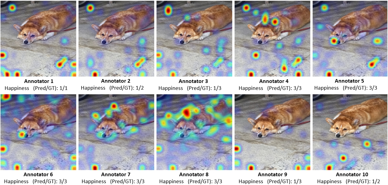
Figure 3. We provide the visualization analysis of the annotator tendencies on the STREET dataset. The focuses of 10 annotators reveal distinct preferences, where annotators 4, 5, 6, 7, and 8 exhibit centralized focuses on a cute dog compared to other annotators.

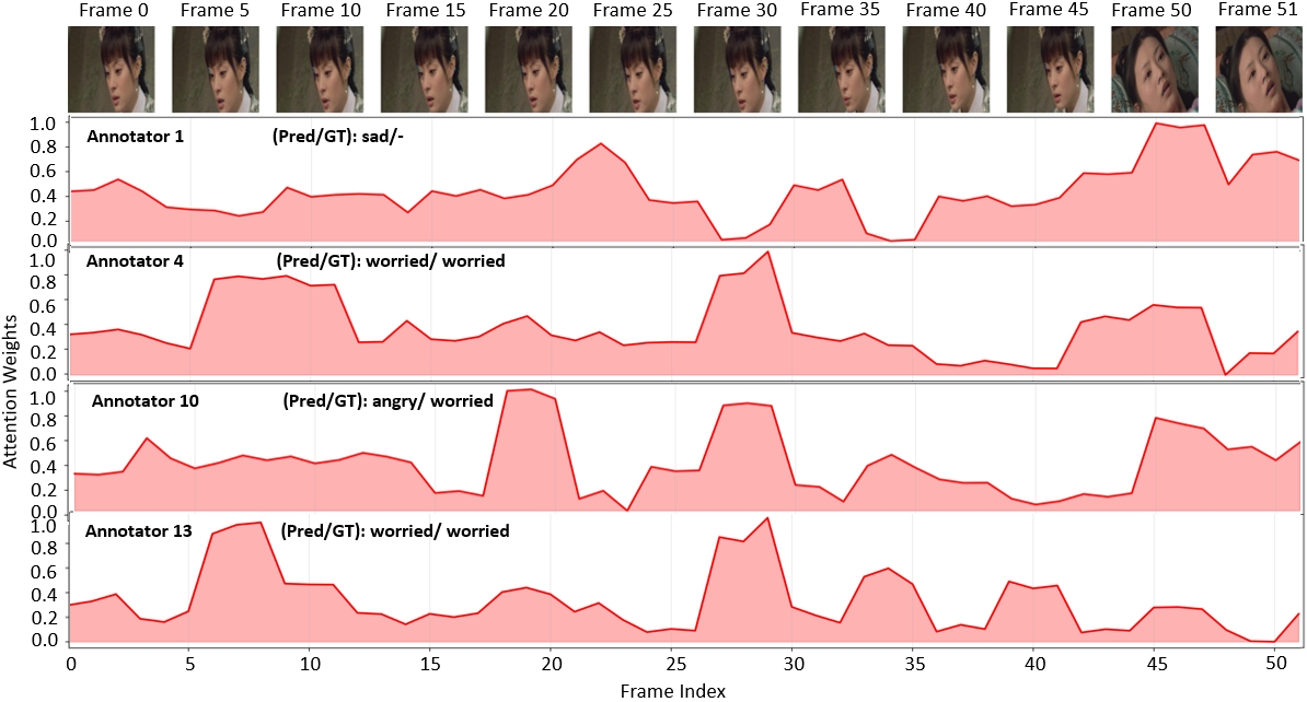
Figure 4. We provide the visualization analysis of the annotator tendencies on the AMER dataset. The annotator 1 exhibits focus on final frames (the frames contain different person), while annotators 4 and 13 focus on the middle frames.

5.2. Evaluation Metrics

For evaluating MATL task, accuracy is the fundamental metric for individual annotator modeling performance. To evaluate how effectively trained models preserve annotators’ tendency information, we propose a new metric, coined difference of inter-annotator consistency (DIC).

Difference of inter-annotator consistency (DIC) quantifies how inter-annotator correlations differ between ground-truths and predictions. To maximize the preservation of annotator tendency information, their correlation coefficients should be close, with smaller differences indicating that the model captures correlations and reflects that the model well preserves the inherent patterns of disagreement among annotators. The annotations given by different annotators differ, and their consistency can be measured by Cohen’s kappa coefficient (Viera and Garrett, 2005). Let $Y_{k}$ and $Y_{l}$ denote the set of all annotations by annotators $A_{k}$ and $A_{l}$. We can compute inter-annotator consistency matrix $M$ whose $(k,l)$-th element $m_{kl}$ is given by

(2) $$m_{kl}=\kappa(Y_{k},Y_{l}),$$

where $\kappa(Y_{k},Y_{l})$ gives Cohen’s kappa coefficient for $Y_{k}$ and $Y_{l}$. We can also compute the inter-annotator consistency matrix $M^{\prime}$ but for predictions $\hat{Y}_{k}$ and $\hat{Y}_{l}$, where its $(k,l)$-th element $m^{\prime}_{kl}$ is given by

(3) $$m^{\prime}_{kl}=\kappa(\hat{Y}_{k},\hat{Y}_{l}).$$

The better the model preserves the tendency information and fits patterns, the smaller the difference between these matrices. We quantify it by

(4) $$\text{DIC}=\|M-M^{\prime}\|_{F},$$

where $\|\cdot\|_{F}$ denotes the Frobenius norm. A lower DIC indicates that the model better preserves the annotator tendency information and successfully captures each annotator’s tendency (with respect to the others).

Table 4. DIC scores to evaluate inter-annotator tendency discrepancy patterns on STREET and AMER datasets, lower values indicate better tendency preservation. -Ha, -He, -Sa, -Li, and -Or represents five perspectives of STREET dataset: happiness, healthiness, safety, liveliness, and orderliness.

Datasets	D-LEMA	PADL	MaDL	Ours
S-Ha	0.62	0.48	0.45	0.43
S-He	0.59	0.52	0.45	0.38
S-Sa	0.36	0.32	0.29	0.24
S-Li	0.51	0.43	0.39	0.27
S-Or	0.61	0.57	0.59	0.54
AMER	0.42	0.36	0.31	0.23

5.3. Quantitative Results

For individual annotator modeling, the accuracy scores in Tables 2 and 3 demonstrate that our method achieves higher scores on both datasets: STREET (covering five perception dimensions: happiness, healthiness, safety, liveliness, and orderliness) and AMER for each annotator. Particularly, our method consistently outperforms other models in terms of average accuracy. In addition, by comparing the results with the Base baseline, it is indicated that the model learned effective annotator information. For inter-annotator consistency, the DIC scores in Table 4 also show that our method surpasses baseline approaches on both STREET and AMER datasets. We indirectly quantify how well the model preserves the annotators’ tendency information through the inter-annotator consistency matrices. These comparative results verify the superiority of our proposed method in modeling individual annotators and the ability to better preserve annotators’ tendency information.

5.4. Qualitative Results

We qualitatively analyze and discuss the visualization of annotator tendencies, which are exhibited by cross-attention weights of Q-former reflecting different focus points of annotators based on their tendencies.

As shown in Figure 3, on the STREET dataset, different annotators’ varying levels of focus on the specific semantics through different patches indicate their tendency differences: annotator 4, 5, 6, 7, and 8 centralized focus more on a cute dog in the image, while other annotators show less focus on this element. This dataset is for city impression emotion classification. Analyzing the annotation and visualization results reveals: annotator 4, 5, 6, 7, and 8 labeled higher scores to the “happiness” dimension, a difference which could potentially be linked to their varying levels of focus on specific semantic of image patches, which might have influenced their judgments. As shown in Figure 4, on the AMER dataset, annotators demonstrate diverse preferences through their varying focus on different frames: annotator 1 shows higher focus on the final frames (45-50), while annotator 4 and 13 focuses more on the early frames (5-10), annotator 10 shows a different focus. This dataset is video emotion classification. Analyzing the annotation and visualization results reveals that annotator 1 predicted “sad”, while annotator 4 and 13 predicted “worried”. The differences in the person or conversations of frame segments they focused on might partially contribute to the variations in their judgments.

Table 5. Ablation study. The average performance of replacing some modules for annotator modeling, removing inter-annotator correlations, as well as a comparison of label aggregation with and without annotator tendency modeling, evaluated by accuracy.

Method	S-Ha	S-He	S-Sa	S-Li	S-Or	AMER
Base	0.42	0.47	0.47	0.53	0.47	0.28
w/ U-cls	0.50	0.56	0.49	0.56	0.49	0.69
w/o S-Attn	0.52	0.54	0.46	0.53	0.56	0.81
Pre-mv	0.62	0.62	0.56	0.58	0.60	0.43
Post-mv	0.62	0.58	0.61	0.59	0.62	0.60
Average	0.63	0.64	0.58	0.62	0.61	0.92

5.5. Ablation Study

We conduct an ablation study for model structure verification. First, we remove Q-Former reducing to the Base model; Second, we only use a unified classifier (w/ U-cls). As shown in Table 5, either of these decreases the overall annotator modeling performance, highlighting their effectiveness in our architecture. To verify the effectiveness of inter-annotator correlations as additional supervision enhancing modeling performance, we remove the self-attention module (w/o S-Attn) in Q-Former. Experimental results show that this decreases the performance, which demonstrates the advantage of capturing inter-annotator correlations in our architecture design. In addition, we also compared the majority voting consensus label training results (Pre-mv) with the majority voting results after modeling individual annotators (Post-mv). For Pre-mv, we perform majority voting on multiple annotator labels to obtain a label $L_{mv}$ and then apply global average pooling on whole queries of Q-Former to a single classifier for end-to-end training to obtain a single inference result $R_{pre}$. For Post-mv, we model annotators’ tendency by learnable queries to independent classifiers for training and then integrate all annotators’ inference results through majority voting to obtain a single result $R_{post}$. Evaluation results comparing $R_{pre}$ and $R_{post}$ with $L_{mv}$ show that Post-mv outperforms Pre-mv overall, validating our insight that modeling tendencies of individual annotators may lead to better specific task results.

6. Conclusion

This paper introduces a new Multi-annotator Tendency Learning (MATL) task, proposes a baseline method QuMATL for this task, provides a new DIC metric, and constructs two large-scale datasets: AMER and STREET. Compared to existing multi-annotator tasks causing the tendency information loss, MATL better preserves the tendency information. Our proposed method captures inter-annotator correlations, which provide an additional supervisory signal from hidden inter-annotator consistency to enhance annotator modeling performance compared to other models. Extensive experiments verified the effectiveness of our method.

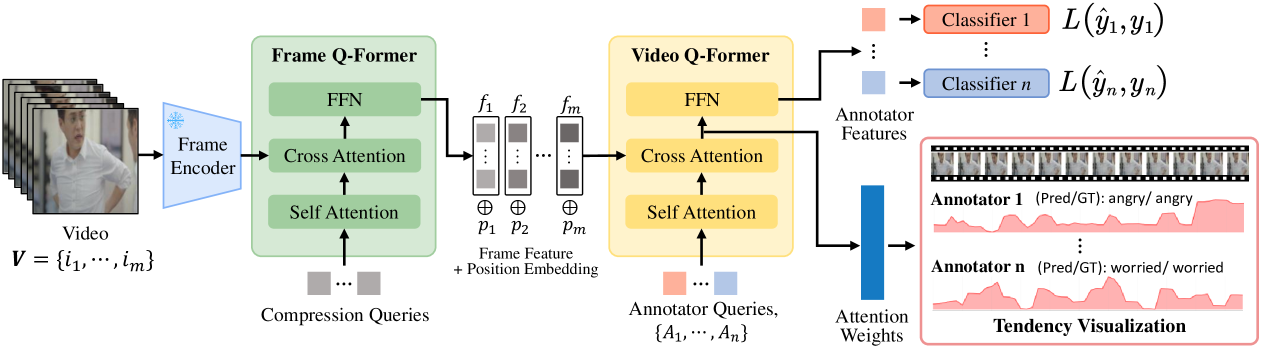
Figure 5. QuMATL architecture for video-specific pipeline. A frozen pre-trained encoder extracts frame features, which are compressed through the Frame Q-Former. With added frame position embedding, these interact with $1,\dots,n$ annotator-specific learnable queries in the Video Q-Former through cross-attention, producing annotator-specific features for classification. Different annotators’ cross-attention weights represent different annotator tendencies and provide visualization for analysis.

7. Supplementary Material

7.1. Overview

In this supplementary, we first illustrate the detailed video-specific architecture in Section 7.2. We provide the analysis of model efficiency in Section 7.3. Also, the extended discussion is provided in Section 7.4. Finally, we show the additional experimental results in Section 7.5.

7.2. Video-specific Architecture

Different from the image input pipeline in the main paper, Figure 5 presents the video input pipeline specifically designed for the AMER, etc. video datasets. Specifically, given a video input $V\in\mathbb{R}^{T\times H\times W\times 3}$, a frozen pre-trained image encoder (Sun et al., 2023) first extracts frame features, which are then further compressed by the image Q-Former using a specific number of compression queries, typically 32, to alleviate subsequent computational costs (Li et al., 2023). The frame position embedding is then added and input to the video Q-Former. Subsequently, we define the unique tendency for annotator $A_{k}$ ($k=1,\dots,n$) through each learnable query in a Q-Former, then all annotator-specific queries in cross-attention simultaneously interact with input features to capture their diverse tendencies and obtain annotator-specific feature. Finally, the specific annotator features are mapped through a fully connected layer to an appropriate feature dimension and then connected to each annotator’s corresponding classifier to output classification results.

For visualization, the focus points to video input are based on all frames of the video. Different annotators’ varying levels of focus on different frames indicate their tendency differences: annotator 1 shows more focus on the final frames, while annotator n focuses more on the middle frames. This dataset is video emotion classification. Analyzing the annotation and visualization results, we see that annotators labeled emotions “anger” and “worried”. The differences in the frame segments they focused on might partially contribute to the variations in their judgments.

Table 6. Model efficiency analysis. In this table, we report the number of parameters and the average inference time per sample. Lower values for both metrics indicate higher model efficiency.

Models	Parameters (M)	Average Processing Time (s)
D-LEMA	$214.18$	$5.64$
PADL	$168.94$	$4.59$
MaDL	$201.37$	$5.06$
Ours	$\bf{106.02}$	$\bf{4.28}$

7.3. Model Efficiency Analysis

This section evaluates the model efficiency from two aspects: model complexity and inference time. For model complexity, we use the number of parameters as the evaluation metric; for inference time, we compute the average processing time per sample. To ensure a fair comparison, Table 6 compares the performance of different methods in the image input pipeline (see Figure 2 in the main paper). Specifically, we evaluate the efficiency of different methods on one perspective of the STREET dataset with 10 annotators. It is worth noting that different methods use different backbone networks. To ensure fairness, we standardize the backbone network to ResNet-34 for all methods. In Table 6, we observe that our model has fewer parameters than the other models, while also maintaining competitive average processing time. This validates our claim in the paper that, compared to the baselines that create separate conventional models for each annotator, our architecture demonstrates significant advantages in model efficiency.

Table 7. Validation randomly deleting labels from STREET and AMER datasets with different proportions for scenarios of sparse continuous annotations per single annotator.

Method	S-Ha	S-He	S-Sa	S-Li	S-Or	AMER
20%-PADL	0.53	0.52	0.46	0.51	0.50	0.80
20%-Ours	0.61	0.60	0.55	0.58	0.59	0.88
30%-PADL	0.48	0.47	0.41	0.46	0.45	0.76
30%-Ours	0.58	0.57	0.52	0.55	0.56	0.85
40%-PADL	0.44	0.42	0.37	0.43	0.41	0.73
40%-Ours	0.55	0.53	0.49	0.52	0.54	0.82
Full-PADL	0.58	0.59	0.52	0.58	0.55	0.87
Full-Ours	0.63	0.64	0.58	0.62	0.61	0.92

7.4. Discussion

We supplement some extended discussions about our work here. First, given that existing multi-annotator datasets often have sparse continuous annotation samples per single annotator, to validate the applicability of our model in these scenarios, we conducted an experiment by randomly deleting labels from AMER and STREET with different proportions, such as 20%, 30%, and 40%. As shown in Table 7, compared to the competing baseline PADL, we maintain superiority across different proportions, with lower performance degradation. Particularly when 40% of labels are deleted, our average performance only decreases by 14%, while PADL decreases by 24%. This superiority may come from our model’s ability to capture inter-annotator correlations during modeling, considering the overall hidden an additional supervisory signal among shared annotators. The experimental results indicate that our model remains effective and applicable to datasets with sparse continuous annotations from single annotators. In the future, we plan to apply and validate it on many other different real-world scenario datasets.

Second, our architecture design superiorly balances effectiveness and complexity, provides an accompanying visualization analysis of annotator tendencies through cross-attention weights. This has potential value and interest for understanding different annotator judgments as described in the main paper. Currently, it is introduced as an accompanying function rather than a main contribution of our paper, but in the future, we hope it can be developed into a mature interpretability solution. We plan to explore to enhance it, which may need pixel-level annotations indicating specific regions that annotators focus on during the annotation process, although this could be expensive. We could also explore quantitative evaluation ways to this further interpretability, such as feature importance ranking consistency, attention-based fidelity metrics, and human intuition consistency assessments through user studies, etc, to further enhance its value and contribution to the community.

Finally, in the ablation study of our main paper, we validated an insight that modeling multiple annotator tendencies can obtain more annotator information and demonstrated its effectiveness through experimental results based on consensus aggregation using majority voting. In future work, we plan to extend more similar experimental scenarios and validations to enhance the explanation of how multi-annotator tendency learning helps and adds benefits to specific applications.

7.5. Additional Results

We provide additional experimental results about visualization analysis of annotator tendencies on both AMER and STREET datasets.

As shown in Figure 6, on the AMER dataset, annotators demonstrate different tendencies through varying focus on different frames. Sample 1 reveals the differences: annotators 5, 10, and 11 show similarly higher focus on the final frames (45-54), while annotator 12 focuses more on middle frames (30-35). They all predict the correct label “happy”, but the different focus positions indicate that annotator 12’s preference pattern for happiness in sample 1 differs from most annotators. Sample 2 shows: annotators 2, 8, and 13 exhibit similarly higher focus on the final frames (45-55), while annotator 12 focuses more on early frames (5-10). They all predict “sad” but annotator 12 demonstrates a different preference pattern.

As shown in Figure 7, on the STREET dataset, annotators exhibit different tendencies through varying focus on different semantic elements within the same input image. In sample 1 from the orderliness perspective, the focus regions show differences: annotator 5 focuses more intensively on graffiti in the image compared with other annotators. The results show that prediction and ground truth are highly consistent in the emotion reflected in the semantics, corresponding to this annotator’s expected lowest score. In sample 2 of the healthiness perspective, most annotators focus on uncleaned garbage and leaves, and only annotator 6 shows more focus on the surrounding environment, like cars and buildings, which might influence the result of not giving a low score.

(a) Sample 1.

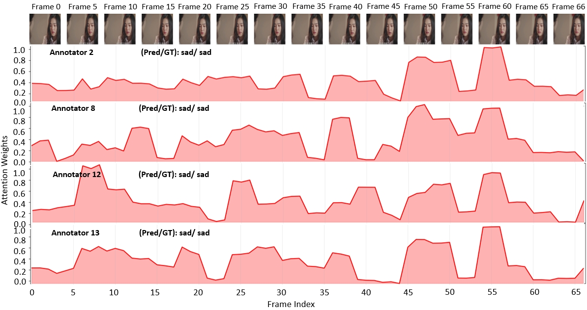
(b) Sample 2.

Figure 6. Additional sample experimental results visualize the annotator tendencies on the AMER video dataset. The tendencies of multi-annotators reveal distinct preferences.

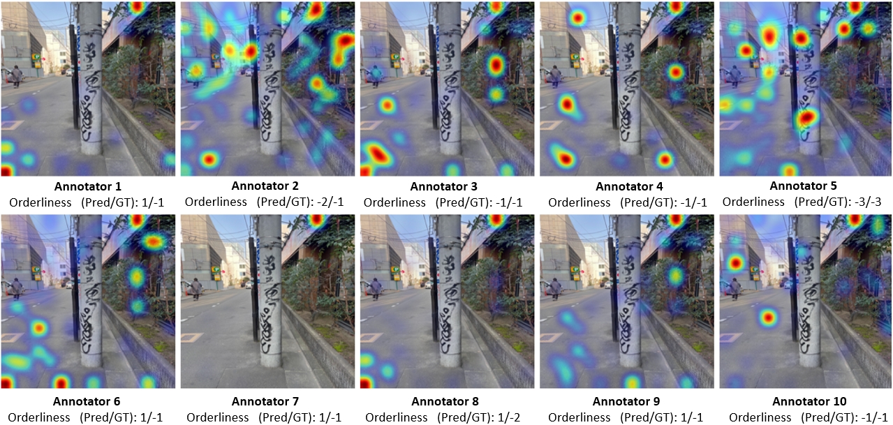
(a) Sample 1 for orderliness perspective.

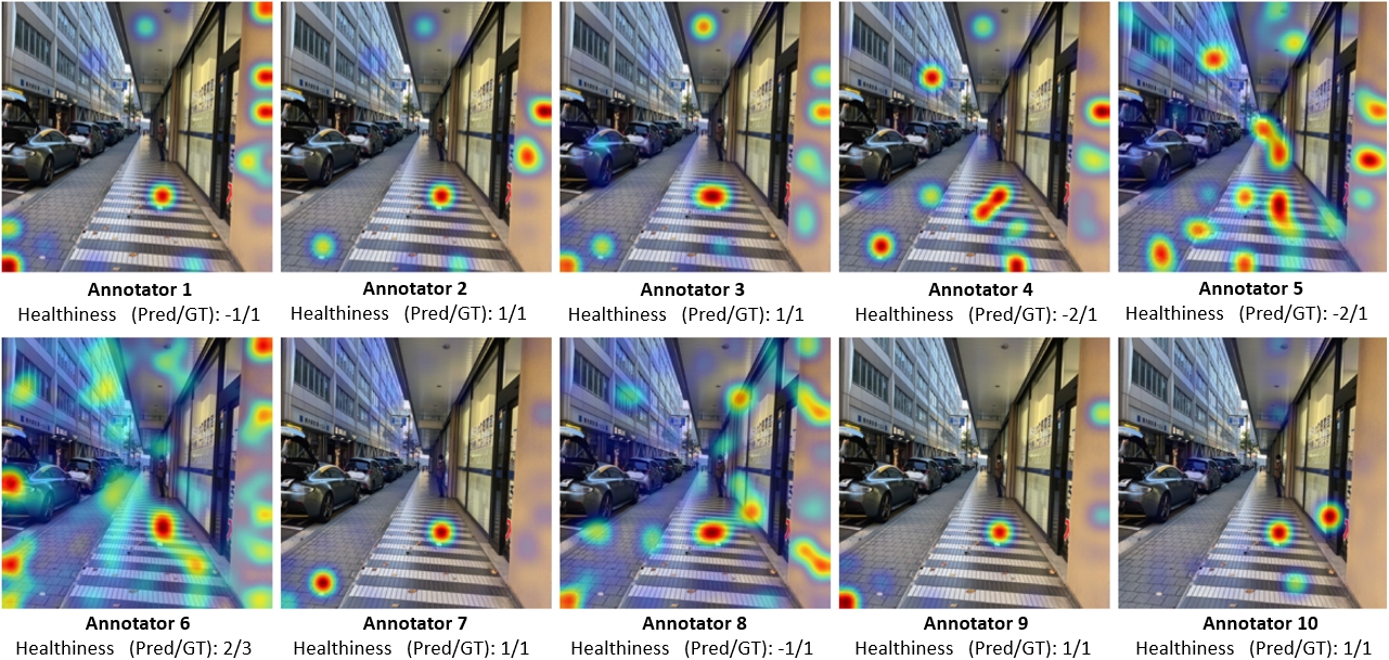
(b) Sample 2 for healthiness perspective.

Figure 7. Additional sample experimental results visualize the annotator tendencies on the STREET image dataset. The tendencies of 10 annotators reveal distinct preferences.

References

- (1)
- Almazroa et al. (2017) Ahmed Almazroa, Sami Alodhayb, Essameldin Osman, Eslam Ramadan, Mohammed Hummadi, Mohammed Dlaim, Muhannad Alkatee, Kaamran Raahemifar, and Vasudevan Lakshminarayanan. 2017. Agreement among ophthalmologists in marking the optic disc and optic cup in fundus images. International ophthalmology 37 (2017), 701–717.
- Armato III et al. (2011) Samuel G Armato III, Geoffrey McLennan, Luc Bidaut, Michael F McNitt-Gray, Charles R Meyer, Anthony P Reeves, Binsheng Zhao, Denise R Aberle, Claudia I Henschke, Eric A Hoffman, et al. 2011. The lung image database consortium (LIDC) and image database resource initiative (IDRI): a completed reference database of lung nodules on CT scans. Medical physics 38, 2 (2011), 915–931.
- Cao et al. (2019) Peng Cao, Yilun Xu, Yuqing Kong, and Yizhou Wang. 2019. Max-mig: an information theoretic approach for joint learning from crowds. arXiv preprint arXiv:1905.13436 (2019).
- Chen et al. (2023) Junfan Chen, Richong Zhang, Jie Xu, Chunming Hu, and Yongyi Mao. 2023. A Neural Expectation-Maximization Framework for Noisy Multi-Label Text Classification. IEEE Transactions on Knowledge and Data Engineering 35, 11 (2023), 10992–11003. https://doi.org/10.1109/TKDE.2022.3223067
- Cheng et al. (2023) Yuan-Chia Cheng, Zu-Yun Shiau, Fu-En Yang, and Yu-Chiang Frank Wang. 2023. TAX: Tendency-and-Assignment Explainer for Semantic Segmentation with Multi-Annotators. arXiv preprint arXiv:2302.09561 (2023).
- Dai et al. (2023) Wenliang Dai, Junnan Li, Dongxu Li, Anthony Tiong, Junqi Zhao, Weisheng Wang, Boyang Li, Pascale Fung, and Steven Hoi. 2023. InstructBLIP: Towards General-purpose Vision-Language Models with Instruction Tuning. In Thirty-seventh Conference on Neural Information Processing Systems. https://openreview.net/forum?id=vvoWPYqZJA
- Dawid and Skene (1979) Alexander Philip Dawid and Allan M Skene. 1979. Maximum likelihood estimation of observer error-rates using the EM algorithm. Journal of the Royal Statistical Society: Series C (Applied Statistics) 28, 1 (1979), 20–28.
- Hashmi et al. (2023) Asma Ahmed Hashmi, Aigerim Zhumabayeva, Nikita Kotelevskii, Artem Agafonov, Mohammad Yaqub, Maxim Panov, and Martin Takáč. 2023. Learning Confident Classifiers in the Presence of Label Noise. arXiv preprint arXiv:2301.00524 (2023).
- Herde et al. (2023) Marek Herde, Denis Huseljic, and Bernhard Sick. 2023. Multi-annotator Deep Learning: A Probabilistic Framework for Classification. arXiv preprint arXiv:2304.02539 (2023).
- Ji et al. (2021) Wei Ji, Shuang Yu, Junde Wu, Kai Ma, Cheng Bian, Qi Bi, Jingjing Li, Hanruo Liu, Li Cheng, and Yefeng Zheng. 2021. Learning calibrated medical image segmentation via multi-rater agreement modeling. In Proceedings of the IEEE/CVF Conference on Computer Vision and Pattern Recognition. 12341–12351.
- Krizhevsky (2009) Alex Krizhevsky. 2009. Learning Multiple Layers of Features from Tiny Images. (Jan 2009).
- Li et al. (2023) Junnan Li, Dongxu Li, Silvio Savarese, and Steven Hoi. 2023. Blip-2: Bootstrapping language-image pre-training with frozen image encoders and large language models. In International conference on machine learning. PMLR, 19730–19742.
- Lian et al. (2023) Zheng Lian, Haiyang Sun, Licai Sun, Kang Chen, Mngyu Xu, Kexin Wang, Ke Xu, Yu He, Ying Li, Jinming Zhao, et al. 2023. Mer 2023: Multi-label learning, modality robustness, and semi-supervised learning. In Proceedings of the 31st ACM International Conference on Multimedia. 9610–9614.
- Lian et al. (2024) Zheng Lian, Haiyang Sun, Licai Sun, Zhuofan Wen, Siyuan Zhang, Shun Chen, Hao Gu, Jinming Zhao, Ziyang Ma, Xie Chen, et al. 2024. MER 2024: Semi-Supervised Learning, Noise Robustness, and Open-Vocabulary Multimodal Emotion Recognition. In MRAC’24: Proceedings of the 2nd International Workshop on Multimodal and Responsible Affective Computing. 41–48.
- Liao et al. (2024) Zehui Liao, Shishuai Hu, Yutong Xie, and Yong Xia. 2024. Modeling annotator preference and stochastic annotation error for medical image segmentation. Medical Image Analysis 92 (2024), 103028.
- Menze et al. (2020) Bjoern Menze, Leo Joskowicz, Spyridon Bakas, Andras Jakab, Ender Konukoglu, Anton Becker, and et al. 2020. Quantification of uncertainties in biomedical image quantification challenge. https://qubiq.grand-challenge.org/.
- Mirikharaji et al. (2021) Zahra Mirikharaji, Kumar Abhishek, Saeed Izadi, and Ghassan Hamarneh. 2021. D-lema: Deep learning ensembles from multiple annotations-application to skin lesion segmentation. In Proceedings of the IEEE/CVF Conference on Computer Vision and Pattern Recognition. 1837–1846.
- Peterson et al. (2019a) Joshua Peterson, Ruairidh Battleday, Thomas Griffiths, and Olga Russakovsky. 2019a. Human uncertainty makes classification more robust. In 2019 IEEE/CVF International Conference on Computer Vision (ICCV). https://doi.org/10.1109/iccv.2019.00971
- Peterson et al. (2019b) Joshua C Peterson, Ruairidh M Battleday, Thomas L Griffiths, and Olga Russakovsky. 2019b. Human uncertainty makes classification more robust. In Proceedings of the IEEE/CVF international conference on computer vision. 9617–9626.
- Rajpurkar et al. (2017) Pranav Rajpurkar, Jeremy Irvin, Aarti Bagul, Daisy Ding, Tony Duan, Hershel Mehta, Brandon Yang, Kaylie Zhu, Dillon Laird, Robyn L Ball, et al. 2017. Mura: Large dataset for abnormality detection in musculoskeletal radiographs. arXiv preprint arXiv:1712.06957 (2017).
- Raykar et al. (2010) Vikas C. Raykar, Shipeng Yu, Linda H. Zhao, Gerardo Hermosillo Valadez, Charles Florin, Luca Bogoni, and Linda Moy. 2010. Learning From Crowds. Journal of Machine Learning Research 11, 43 (2010), 1297–1322. http://jmlr.org/papers/v11/raykar10a.html
- Rodrigues and Pereira (2018) Filipe Rodrigues and Francisco Pereira. 2018. Deep learning from crowds. In Proceedings of the AAAI conference on artificial intelligence, Vol. 32.
- Rodrigues et al. (2013a) Filipe Rodrigues, Francisco Pereira, and Bernardete Ribeiro. 2013a. Learning from multiple annotators: distinguishing good from random labelers. Pattern Recognition Letters 34, 12 (2013), 1428–1436.
- Rodrigues et al. (2013b) Filipe Rodrigues, Francisco Pereira, and Bernardete Ribeiro. 2013b. Learning from multiple annotators: distinguishing good from random labelers. Pattern Recognition Letters 34, 12 (2013), 1428–1436.
- Rodrigues et al. (2014) Filipe Rodrigues, Francisco Pereira, and Bernardete Ribeiro. 2014. Gaussian Process Classification and Active Learning with Multiple Annotators. In Proceedings of the 31st International Conference on Machine Learning (Proceedings of Machine Learning Research, Vol. 32), Eric P. Xing and Tony Jebara (Eds.). PMLR, Bejing, China, 433–441. https://proceedings.mlr.press/v32/rodrigues14.html
- Schaekermann et al. (2019) Mike Schaekermann, Graeme Beaton, Minahz Habib, Andrew Lim, Kate Larson, and Edith Law. 2019. Understanding Expert Disagreement in Medical Data Analysis through Structured Adjudication. Proc. ACM Hum.-Comput. Interact. 3, CSCW, Article 76 (Nov. 2019), 23 pages. https://doi.org/10.1145/3359178
- Sun et al. (2023) Quan Sun, Yuxin Fang, Ledell Wu, Xinlong Wang, and Yue Cao. 2023. Eva-clip: Improved training techniques for clip at scale. arXiv preprint arXiv:2303.15389 (2023).
- Tanno et al. (2019a) Ryutaro Tanno, Ardavan Saeedi, Swami Sankaranarayanan, Daniel C. Alexander, and Nathan Silberman. 2019a. Learning From Noisy Labels by Regularized Estimation of Annotator Confusion. In Proceedings of the IEEE/CVF Conference on Computer Vision and Pattern Recognition (CVPR).
- Tanno et al. (2019b) Ryutaro Tanno, Ardavan Saeedi, Swami Sankaranarayanan, Daniel C Alexander, and Nathan Silberman. 2019b. Learning from noisy labels by regularized estimation of annotator confusion. In Proceedings of the IEEE/CVF conference on computer vision and pattern recognition. 11244–11253.
- Tkachenko et al. (2025) Maxim Tkachenko, Mikhail Malyuk, Andrey Holmanyuk, and Nikolai Liubimov. 2020-2025. Label Studio: Data labeling software. https://github.com/HumanSignal/label-studio Open source software available from https://github.com/HumanSignal/label-studio.
- Viera and Garrett (2005) AnthonyJ. Viera and JoanneM. Garrett. 2005. Understanding interobserver agreement: the kappa statistic. Family Medicine,Family Medicine (May 2005).
- Wang et al. (2023) Chongyang Wang, Yuan Gao, Chenyou Fan, Junjie Hu, Tin Lum Lam, Nicholas D Lane, and Nadia Bianchi-Berthouze. 2023. Learn2agree: Fitting with multiple annotators without objective ground truth. In International Workshop on Trustworthy Machine Learning for Healthcare. Springer, 147–162.
- Welinder et al. (2010) Peter Welinder, Steve Branson, Pietro Perona, and Serge Belongie. 2010. The multidimensional wisdom of crowds. Advances in neural information processing systems 23 (2010).
- Whitehill et al. (2009) Jacob Whitehill, Ting-fan Wu, Jacob Bergsma, Javier Movellan, and Paul Ruvolo. 2009. Whose vote should count more: Optimal integration of labels from labelers of unknown expertise. Advances in neural information processing systems 22 (2009).
- Zhang et al. (2023b) Hang Zhang, Xin Li, and Lidong Bing. 2023b. Video-LLaMA: An Instruction-tuned Audio-Visual Language Model for Video Understanding. In Proceedings of the 2023 Conference on Empirical Methods in Natural Language Processing: System Demonstrations. 543–553.
- Zhang et al. (2023c) Le Zhang, Ryutaro Tanno, Moucheng Xu, Yawen Huang, Kevin Bronik, Chen Jin, Joseph Jacob, Yefeng Zheng, Ling Shao, Olga Ciccarelli, et al. 2023c. Learning from multiple annotators for medical image segmentation. Pattern Recognition 138 (2023), 109400.
- Zhang et al. (2023a) Yifei Zhang, Siyi Gu, Yuyang Gao, Bo Pan, Xiaofeng Yang, and Liang Zhao. 2023a. Magi: Multi-annotated explanation-guided learning. In Proceedings of the IEEE/CVF International Conference on Computer Vision. 1977–1987.