Sig2text, a Vision-language model for Non-cooperative Radar Signal Parsing

Abstract

Automatic non-cooperative analysis of intercepted radar signals is essential for intelligent equipment in both military and civilian domains. Accurate modulation identification and parameter estimation enable effective signal classification, threat assessment, and the development of countermeasures. In this paper, we propose a symbolic approach for radar signal recognition and parameter estimation based on a vision-language model that combines context-free grammar with time-frequency representation of radar waveforms. The proposed model, called Sig2text, leverages the power of vision transformers for time-frequency feature extraction and transformer-based decoders for symbolic parsing of radar waveforms. By treating radar signal recognition as a parsing problem, Sig2text can effectively recognize and parse radar waveforms with different modulation types and parameters. We evaluate the performance of Sig2text on a synthetic radar signal dataset and demonstrate its effectiveness in recognizing and parsing radar waveforms with varying modulation types and parameters. The training code of the model is available at https://github.com/Na-choneko/sig2text.

1 Introduction

Automatic non-cooperative analysis of intercepted radar signals is essential for intelligent equipment in both military [32] and civilian domains [17, 2]. Accurate modulation identification and parameter estimation enable effective signal classification, threat assessment, and the development of countermeasures. However, the increasing prevalence of software-defined radar systems [12, 4] has introduced new challenges. Modern radar systems now employ advanced techniques such as low power transmission, spread spectrum methods, frequency agility, and complex modulation schemes, which complicate the detection and analysis of radar signals [19, 22].

Traditional approaches for radar signal intra pulse modulation recognition and parameter estimation primarily relied on statistical signal processing techniques. The modulation recognition often involves signal feature extraction followed by classification using statistical pattern recognition algorithms. For example, [16] extracted a set of features from Wigner and Choi–Williams time-frequency distributions of intercepted signals and then pruned redundant ones using an information-theoretic approach. In [31] signals are decomposed into time-frequency atoms via a fast matching pursuit algorithm to enabled robust clustering of radar emitter signatures. In [18, 27], decision-theoretic frameworks and statistical tests are introduced for intrapulse modulation recognition. For parameter estimation, For parameter estimation, several methods have been developed that address the challenges of low signal-to-noise ratios and the inherent complexity of modern radar signals. In [6], a cyclostationary approach is employed to extract key modulation parameters of low probability of intercept (LPI) radar signals, achieving estimation errors well below 6% and demonstrating improved performance over traditional methods. Similarly, the work in [3] reformulates chirp rate estimation as a series of frequency estimation problems through the use of multiple discrete polynomial phase transforms (DPT) combined with an optimal weighting strategy. In addition, [22] presents a framework that integrates time-frequency representations with visibility graph techniques to enhance the detection and estimation of multicomponent LPI radar signals. Despite the effectiveness of these methods, they often rely on handcrafted features for specific signal types and can not adapt to newly emerging signals with complex modulation schemes.

With the rapid advancement of deep learning techniques, numerous approaches have been developed. These methods can be roughly categorized based on their input: those that directly process sampled sequence from analog-to-digital convertor (ADC) and those that utilize time-frequency image representations. The sequence-based approaches directly input the sampled radar signals into the neural networks for timeseries, which then automaticly learns to extract features and classify the modulation type. For example, convolutional neural networks (CNNs) and long short-term memory (LSTM) networks and their variant have been studied in [14, 25, 21, 26] and promising results were shown. The time-frequency image(TFI)-based approaches first transform the radar signals into time-frequency images, which are then fed into the neural networks that processing images for feature extraction and classification. Methods with special desinged achitectures [13, 20, 10, 11] have been proposed and promising results were also shown. In the simulations section, we will compare the sequence-based and image-based network architecture in detail.

The above metioned methods can only recognize the intra-pulse modulations and modulation parameter estimation is not performed. To address this issue, multi-task learning has been introduced. Akyön et al. [1] proposed a multi-task learning and recurrent neural network-based technique for joint SNR estimation, pulse detection, and modulation classification. Zhu et al. [30] proposed JMRPE-Net, a deep multitask network for joint modulation recognition and parameter estimation of cognitive radar signals, which can process sequences of radar pulse signals and perform multiple tasks in parallel. For overlapped signals, Chen et al. [5] developed a joint semantic learning deep convolutional neural network, which jointly performs feature restoration, modulation classification, and parameter regression. However, those model usually have fixed number of output heads, which can not adapt to radar signals with varying number of parameters and types (e.g radar signals with complex hybrid modulations).

In this paper, we propose a symbolic approach for radar signal recognition and parameter estimation based on a vision-language model that combines context-free grammar(CFG) with time frequency representation of radar waveforms. The proposed model, called Sig2text, leverages the power of vision transformers for time-frequency feature extraction and transformer-based decoders for symbolic parsing of radar waveforms. By treating radar signal recognition as a parsing problem, Sig2text can effectively recognize and parse radar waveforms with different modulation types and parameters. We evaluate the performance of Sig2text on a synthetic radar signal dataset and demonstrate its effectiveness in recognizing and parsing radar waveforms with varying modulation types and parameters.

2 Problem formulation

2.1 Signal Model

For a non-cooperative radar signal receiver, the signal $y(k)$ with additive Gaussian white noise (AWGN) after sampling can be modeled as:

$$y(k)=A*\exp\left(j\cdot\left(\theta(k)+2\pi\frac{f_{c}}{f_{s}}k\right)+\theta_{p}\right)+n(k)$$ (1)

where , $A$ is the amplitude of the signal that is constant within the pulse width, $\theta(k)$ is the instantaneous phase of the signal, $f_{c}$ is the carrier frequency, $f_{s}$ is the sampling frequency, $\theta_{p}$ is the phase offset, and $n(k)$ is the AWGN.

Based on the instantaneous phase $\theta(k)$, basic radar signals can roughly be categorized into three types: frequency modulated (FM), phase coded (PC), and frequency coded (FC) waveforms [4]. FM waveforms use continuous phase modulation to achieve pulse compression, with linear frequency modulation (LFM) being a common example. PC waveforms subdivide the pulse into constant-amplitude chips each modulated by discrete phase values (either binary or polyphase). FC waveforms modulates its frequency in a predetermined stepped-frequency sequences, with Costas codes being a common example. Table 1 shows the basic radar waveforms and some of their subclasses.

Table 1: Basic radar waveforms and their some of their subclasses

Waveform Type	Subclasses
FM	LFM, Triangular Waveform (Tri)
PC	Barker, Polyphase, Frank, P1, P2, P3, P4
FC	Costas

In addition to the basic waveforms, radar signals in practice can involve hybrid modulations. For example, FM and PC waveforms can be combined to create signals like LFM/binary phase shift keying (BPSK) to achieve low probability of interception. And FC and PC waveforms can be combined to achieve effective jamming suppression[9]. Even multiple LFM with different slops can be combined to achieve better velocity estimation for Synthetic Aperture Radar(SAR)[29].

Because of the uncertain number of signal with exponential number of combinations, the task of radar signal analysis can no longer be viewed as a simple classification or regression problem. Instead, we formulate it as a parsing problem from signal domain to the symbolic domain, which will be described in the next section.

2.2 The task of radar signal parsing

Just like humans can use natural language with finite alphabet to describe the content of any images, a language can be defined to describe the content of a radar signal. Formally, Let $\Sigma$ be a finite alphabet, i.e., a finite set of symbols. The set of all finite strings over a alphabet $\Sigma$ is defined as

$$\Sigma^{*}=\bigcup_{n=0}^{\infty}\Sigma^{n},$$

where $\Sigma^{n}$ denotes the set of all strings of length $n$ (with $\Sigma^{0}=\{\varepsilon\}$, where $\varepsilon$ is the empty string). A formal language is any subset of $\Sigma^{*}$:

$$L\subseteq\Sigma^{*}.$$

Despite the finite nature of the alphabet $\Sigma$, the set $\Sigma^{*}$ is infinite because symbols can be concatenated arbitrarily. This inherent property endows formal languages with vast expressive power, as it allows the encoding of an unbounded amount of information. Moreover, many formal languages are defined by grammars that incorporate recursive production rules, enabling the construction of nested and hierarchical structures essential for representing complex syntactic patterns.

With the language, we can formalize radar signal parsing as a mapping from a continuous signal domain to a discrete symbolic domain. Let a radar signal be represented by a vector

$$I\in\mathbb{R}^{N\times 1},$$

where $N$ denotes the total number of sample points. Define a finite alphabet (i.e., the vocabulary) $\Sigma$, and consider the set of all finite strings over $\Sigma$, denoted by $\Sigma^{*}$. The corresponding symbolic description of the radar signal is modeled as a sequence (or string)

$$T=(w_{1},w_{2},\dots,w_{n})\in\Sigma^{*},$$

with each symbol $w_{t}\in\Sigma$. Our goal is to learn a mapping

$$f:\mathbb{R}^{N\times 1}\rightarrow\Sigma^{*}$$

by maximizing the conditional probability $P(T\mid I)$. Applying the chain rule, this probability can be factorized as

$$P(T\mid I)=\prod_{t=1}^{n}P\bigl{(}w_{t}\mid I,w_{1},\dots,w_{t-1}\bigr{)}.$$

Therefore, the parsing problem can be viewed as a conditional, next token prediction task, and the learning of the mapping $f$ is converted to the estimation of the conditional probability $P(w_{t}\mid I,w_{1},\dots,w_{t-1})$, which can be achieved by training a neural network.

The choice of the types of the language is crucial for clear and concise representation of radar signals and in the next section, we will describe how this is achieved with a special designed language that can represent arbitrary radar waveforms with different parameters.

3 Method

In this section we first describe the symbolic representation of radar waveforms, and then introduce the vision transformer architecture for time-frequency feature extraction and transformer-based decoders for symbolic parsing of radar waveforms.

3.1 Symbolic representation of radar waveforms

In this section, we describe an artificial language that can represent arbitrary radar waveforms with different parameters, so that the recognition and parameter estimation of radar waveforms can be viewed as a language parsing problem.

The first question is how to choose the types of the language. A naive approach is to use natural language to describe the radar signals, but this approach is not efficient because the natural languages(such as English and Chinese) have vast amount of vocabulary, which is too expressive and can not be easily parsed by the machine. Observe that the radar signals have a limited number of types and parameters, we artificially design a language with CFG.

CFG is a formal grammar in which every production rule is of the form $A\rightarrow\alpha$, where $A$ is a non-terminal symbol and $\alpha$ is a string of terminal and/or non-terminal symbols. The language generated by a CFG is the set of strings that can be derived from the start symbol by applying a sequence of production rules. For example, the CFG $G=(\{S\},\{a,b\},\{S\rightarrow aSb,S\rightarrow\epsilon\},S)$ generates the language $\{a^{n}b^{n}|n\geq 0\}$, which consists of all strings of the form $a^{n}b^{n}$. With a few simple rules, CFG can generate complex languages, which has been used in image processes [7] and Multifunction Radar modeling [24].

In our applications, for basic waveforms such as FM waveform, phase code, and frequency code, the string representations have the following forms: <type> <sub> <parameter_list>. The type field represents the major category of signal modulation, which only contain ’FM’,’PC’,’FC’, sub_type represents the subcategory of signal modulation under each major category, for example, ’backer’ is a valid subtype under the major category ’PC’. The parameter_list field represents a list of parameters of the signal such as bandwidth, carrier frequency, code sequence, etc. An exemplar grammar for the language is shown in Table 2. For example, suppose the unit of frequency is MHZ, the string FM LFM cf 100.0 B 10.0 represents a linear frequency modulated waveform with a center frequency of 100.0 MHz and a bandwidth of 10.0 MHz. The string FC Costas cf 100.0 FH 1.0 Code 7 6 2 10 1 4 8 9 11 5 3 represents a frequency code waveform with a Costas code sequence, a center frequency of 100.0 MHz, a frequency hop of 1.0 MHz, and a code sequence of 7 6 2 10 1 4 8 9 11 5 3.

Table 2: Simple grammar Rules that describe 5 basic radar waveforms:LFM, P1, P2, P4, CostasFM. The terminal symbols are defined as follows: $<FM>$,$<PM>$,$FC$,$<P1>$, $<P2>$, $<P4>$, $<Costas>$, $<LFM>$ are the waveform types, $<cf>$, $<B>$, $<FH>$, $<Code>$ are the parameter that need to be estimated, $<FLOAT>$ $<INT>$ represent specific value of a parameter.

Non-terminal	Productions
$<ENTRY>$	$<FM\_ENTRY>\mid<PM\_ENTRY>\mid<FC\_ENTRY>$
$<FM\_ENTRY>$	$<FM><LFM><cf><FLOAT><B><FLOAT>$
$<PM\_ENTRY>$	$<PM><P\_TYPE><cf><FLOAT><code\_length><INT>$
$<FC\_ENTRY>$	$<FC><Costas><cf><FLOAT><FH><FLOAT><Code><INT\_LIST>$
$<P\_TYPE>$	$<P1>\mid<P2>\mid<P4>$
$<INT\_LIST>$	$<INT><INT\_LIST>\mid<INT>$

For composite waveforms, we could recursively use the grammar rules by adding another production rule $<S>\rightarrow<ENTRY><S>\mid<ENTRY>$. For example, the string FM LFM cf 100.0 B 10.0 PM P1 cf 100.0 code_length 10 represents a radar signal that is a combination of a linear frequency modulated waveform with phase modulated waveform, the carrier frequency is 100.0 MHz, the bandwidth is 10.0 MHz and the code length is 10. Notice the carrier frequency has been repeated in the string, which is not a problem because in the parsing process, we will only keep the first occurrence of the carrier frequency.

One futher step needs to be applied to the string representation is to convert the continuous values (e.g $<FLOAT>$) in to discrete tokens, because the decoder can only output discrete tokens. Depending on the measurement range and expected precision of the continuous values, we can use different size of quantization unit. The quantization process can be done by simply dividing the continuous value by the quantization unit and rounding to the nearest integer. Take the bandwidth parameter as an example, if the range is between 0 and 100MHZ, and the quantization unit is 0.1, for signals with 23.43MHZ bandwidth, the quantized representation will be $234$.

3.2 Architecture of Sig2text

In this study, to make the learned features more interpretable, and robust to noise, we apply Time-frequency Transform to the radar waveforms before feeding to the encoders. Specifically, for computational efficiency, we use Short-Time Fourier Transform (STFT) for feature extraction. Because the phase of the STFT contain less useful information, we only use the magnitude of the STFT, resulting a time-frequency image of one channel.

In previous studies, Convolutional Neural Networks (CNNs) have been widely used for recognizing time-frequency images of radar waveforms. However, the receptive fields of CNNs are limited by the size of the convolutional kernels, which makes it difficult for CNNs to capture long-range dependencies in the input image. To address this issue, we propose to use the Vision Transformer (ViT) [8] . The ViT is a transformer-based model that has been shown to be effective for image processing tasks. The ViT divides the input image into patches and processes them using a transformer encoder. The transformer encoder captures the long-range dependencies in the input image by allowing each patch to attend to all other patches. The ViT has been shown to outperform CNNs on several image processing tasks such as recognition, segmentation and [28] .

Suppose the size the time-frequency image is of size $N\times M$, we divide the whole image into patches of size $n\times m$, where $n$ is the number of time bins and $m$ is the number of frequency bins. Additionally, $n$ is a divisor of $N$, and $m$ is a divisor of $M$. This flexible choice of patch size allows the model to adapt to the varying time-frequency images generated by waveforms with different pulse widths. Each patch is then flattened into a vector and linearly projected into a $D$ dimensional embedding space. The resulting vectors are of size $\mathbb{R}^{\left(\frac{N}{n}\times\frac{M}{m}\right)\times D}$, which are then used as input to the Transformer model.

Since the attention blocks in the Transformer model contain no inherent positional information, we add a learnable positional encoding to the input vectors. In detail, a parameter matrix $P\in\mathbb{R}^{L\times D}$ is initialized, where $L=\left(\frac{N}{n}\times\frac{M}{m}\right)$ is the total number of patches and $D$ is the dimension of the projected patch vectors. Each row of $P$ corresponds to a unique positional embedding that is added element-wise to its corresponding patch vector. During training, these embeddings are optimized along with the rest of the model, allowing the network to learn an appropriate spatial representation that informs the Transformer about each patch’s position within the original time-frequency image.

The backbone of the encoder is a stack of $L$ identical layers, each containing a multi-head self-attention layer followed by a layer with normalization, just like standard transformer[23]. The output of the final layer is then passed to a linear layer that maps the output to a $K$-dimensional vector, which served as the input to the decoder for parsing.

Just like standard transformer[23], the decoder consists of $L$ identical layers, each containing a masked multi-head self-attention layer followed by a layer with normalization. Except that a residual connection is added between the embedding and each decoder layer. The output of the final layer is then passed to a linear layer that maps the output to a $K$-dimensional vector, which is then used to predict the next token in the sequence. The overview of the Sig2text architecture is shown in Figure 1, which demonstrates the process of converting raw sequence input into tokens using encoder and decoder blocks.

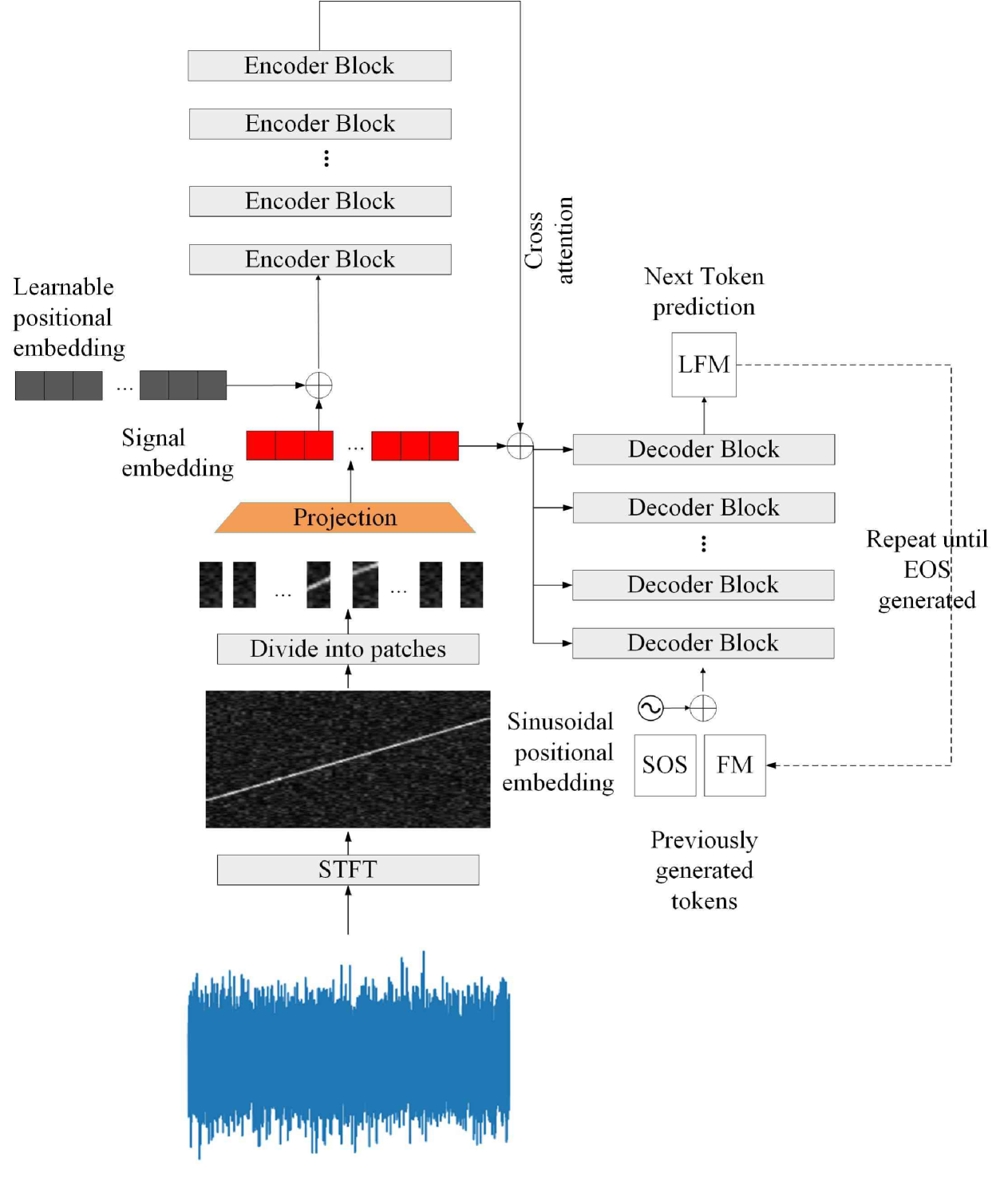
Figure 1: An overview of Sig2text architecture.

3.3 Training and inference

Given a set of sampled radar signals $x^{(1)},x^{(2)},...,x^{(N)}$, and their corresponding symbolic representation $s^{(1)},s^{(2)},...,s^{(N)}$, our learning objective is to learn the model parameter $\theta$ that maximize the likelihood of the string $s^{(i)}$ given the input $x^{(i)}$. Specifically, the log-likelihood function is defined as:

$$\mathcal{L}(\theta)=\frac{1}{N}\sum_{i=1}^{N}\log p_{\theta}(s^{(i)}|x^{(i)})$$ (2)

, where $\theta$ is the set of parameters of the model. However, directly maximizing the log-likelihood function can be inefficient because it requires the model to predict all the preceding tokens in the sequence autoregressivly. To address this issue, we use the teacher forcing technique. The idea is to use the ground truth tokens as input to the decoder during training, instead of using the predicted tokens. With teacher forcing, the final learning objective becomes:

$$loss(\theta)=-\frac{1}{N}\sum_{i=1}^{N}\sum_{t=1}^{T_{i}}\log p_{\theta}(s_{t}^{(i)}|s_{1}^{(i)},...,s_{t-1}^{(i)},x^{(i)})$$ (3)

, where $T_{i}$ is the length of the string $s^{(i)}$, and $p_{\theta}(s_{t}^{(i)}|s_{1}^{(i)},...,s_{t-1}^{(i)},x^{(i)})$ is the probability of the $t$-th token in the string given the previous tokens and the input sample. With the negative log-likelihood function, we can use gradient descent to update the model parameters. The full training procedure is shown in Algorithm 1. Notice two special tokens $<sos>$ and $<eos>$ are added to the beginning and the end of the string, respectively. The $<sos>$ token is used to indicate the beginning of the string, and the $<eos>$ token is used to indicate the end of the string.

Algorithm 1 Training Procedure

0: Training data $\mathcal{D}=\{(x^{(i)},s^{(i)})\}_{i=1}^{N}$, learning rate $\eta$, number of epochs $E$, batch size $B$

1: Quantization of continuous values in $s^{(i)}$ to discrete tokens

2: Add start token $<sos>$, end token $<eos>$ to each string, and build vocabulary from the training data.

3: for $epoch=1,\dots,E$ do

4:  for each mini-batch $\mathcal{B}\subset\mathcal{D}$ do

5:   Compute the magnitude specturm of STFT from input signal $x$

6:   Divide time-frequency image into patches and project into $D$-dimensional embeddings

7:   Add learnable positional encodings to patch embeddings

8:   Forward pass through the Transformer encoder to obtain latent representation

9:   Use Transformer decoder to predict the distribution of the next token

10:   Compute negative log-likelihood loss (same as the cross-entropy loss)

11:   Backpropagate and update model parameters using gradient descent with learning rate $\eta$

12:  end for

13:  Optionally: Validate model performance on a held-out set

14: end for

During inference, we use beam search decode to predict the string from the input sample.The algorithm maintains a fixed-size beam of the most promising results. Suppose the size of beam width is $K$, at each level, the algorithm expands all nodes in the beam and selects the $K$ most promising nodes to form the new beam. The process is repeated until the end of the string is reached. The full inference procedure is shown in Algorithm 2.

Algorithm 2 Inference Procedure

0: Input signal $x$, beam width $K$, maximum length of the string $T_{max}$

1: Compute the magnitude specturm of STFT from input signal $x$

2: Divide time-frequency image into patches and project into $D$-dimensional embeddings

3: Add learnable positional encodings to patch embeddings

4: Forward pass through the Transformer encoder to obtain latent representation

5: Initialize the beam with the start token $<sos>$

6: for $t=1,\dots,T_{max}$ do

7:  for each node in the beam do

8:   Use Transformer decoder to predict the next token

9:   Compute the log-likelihood of the predicted token

10:   Add the predicted token to the node

11:  end for

12:  Select the $K$ most promising nodes to form the new beam

13:  if any node in the beam ends with $<eos>$ then

14:   Break

15:  end if

16: end for

17: Select the string corresponding to the node with the highest log-likelihood and convert it back to the types and parameters of the radar waveform.

4 Simulations

In this section, we evaluate the performance of the proposed Sig2text model on a synthetic radar signal dataset. We compare the performance of Sig2text on both type recognition and parameter estimation on a data set containing 13 signal classes. We also investigate the transfer learning ability of the model by training on a dataset with complex hybrid modulations.

4.1 Dataset description

In this section we describe the synthetic datasets used to evaluate the performance of different models. The dataset is generated using a radar simulator written in CUDA, which models the whole transmission and receiving chain. The sampling frequency of the receiver is set to 100MHZ and the pulse width of each pulse is between 50us and 100us. Due to different Effective Radiated Power(ERP) and distance from the emitter to the receiver, the signal-to-noise ratio (SNR) of the signals varies from -10dB to 10dB. The first dataset contains 500,000 samples evenly distributed across 13 classes, including LFM, sinusoidal(Sin) frequency modulation, Triangular frequency modulation, Frank , P1 to P4,T1 to T4 and Costas FC. The modulation parameters are randomly generated within a certain range, which is shown in Table 3.

Table 3: Approximate Parameter Ranges for LPI Signals

Parameter	Range	Remarks	Description
$cf$	10–40 MHz	All signal types	Center frequency
$B$	2–10 MHz	LFM: 2–10; Sin/Tri: 10–20	Signal bandwidth
$T$	5–20 $\mu$s	Sin/Tri signals	Modulation period
$FH$	$\geq$0.5 MHz	Costas; upper limit depends on Code	Frequency hop step
segment_num	1–4	T1/T2/T3/T4	Number of segments
phasestate_num	2–4	T1/T2/T3/T4	Number of phase states
$\Delta F$	1–10 MHz	T3/T4	Modulation bandwidth
code_length	3-10	P1/P2/P3/P4	Phase code length
Code	-	Costas	Costas sequences

The second dataset contains 10000 samples with complex hybrid modulations, which are generated by combining two basic waveforms from the first dataset. The possible ways of combinations are summarized in Table 4.

Table 4: Summary of Hybrid Modulation Types

Hybrid Type	Subtypes	Ways of combinations
FM+FM	Multiple LFM	Sequential combinations
FM+PM	LFM + Polyphase (P1-4, T1-4, Frank)	Multiplicative combinations
FM+FC	LFM + Costas	Multiplicative combinations
PM+FC	Polyphase (P1-4, T1-4, Frank) + Costas	Multiplicative combinations
PM+PM	Two Polyphase (P1-4, Frank)	Sequential combinations

4.2 Hyperparameters and Baseline Methods

In this section, we describe the hyperparameters used in the experiments and the baseline methods used for comparison.

Because none of the existing approaches can perform complete signal recognition and parameter estimation on the second dataset, we only compare full functionality of the proposed method with the baseline methods on the first dataset. And for the second dataset, we only compare the recognition performance. The selected baseline methods are as follows:

• JMRPE-Net[30]: A deep multi-task network combined with the CNN, LSTM and self-attention modules. The model is trained with to jointly recognize the modulation type and estimate the modulation parameters of radar signals.

• MTViT: A vision transformer encoder same as the proposed model, but with a fixed number of output heads. The model is for Ablation Study.

And the hyperparameters of the proposed model and the baseline methods are shown in Table 5.

Table 5: Key component hyperparameters across the three network architectures

Layers	JMRPENet	MTVit	Sig2text
CNN	3 layers (1,64,7) → (64,128,5) → (128,256,3)	-	-
LSTM	Bidirectional Input: 256 Hidden: 128	-	-
Attention	8-head Hidden: 256	8-head Hidden: 128	8-head Hidden: 128
Transformer Encoder	-	Layers: 3 Hidden: 128 FF size: 512	Layers: 6 Hidden: 128 FF size: 1024
Transformer Decoder	-	-	Layers: 6 Hidden: 128 FF size: 1024

For Sig2text, we define the following CFG rules to describe the 13 basic radar waveforms along with the hybrid modulations. The CFG rules are shown in Table 2. Using those rules, we generate symbolic strings that describe the radar signals based on its parameters and types. For continuous values in the generated strings, we use a quantization unit of 0.01.

Table 6: CFG Productions that describe basic radar waveforms and their hybrid modulations. In the productions, the strings enclosed by " ", along with the ’Number’ are the terminal symbols that will ultimately appear in the radar signal symbolic representation.

Non-Terminal	Production Rule
$S$	$SimpleString\mid CompoundString$
$SimpleString$	$TypeChoice\ SubTypeChoice\ para$
$CompoundString$	$CompoundTypeChoice\ SimpleString\ SimpleString$
$TypeChoice$	"FM" $\mid$ "PM" $\mid$ "FC"
$CompoundTypeChoice$	"FM-FM" $\mid$ "FM-PM" $\mid$ "FM-FC" $\mid$ "PM-FC" $\mid$ "PM-PM"
$SubTypeChoice$	"LFM" $\mid$ "Sin" $\mid$ "Tri" $\mid$ "Costas" $\mid$ "T1" $\mid$ "T2" $\mid$ "T3" $\mid$ "T4" $\mid$ "P3" $\mid$ "P4" $\mid$ "P1" $\mid$ "P2" $\mid$ "Frank"
$para$	$LFMpara\mid SinTripara\mid Costaspara\mid T12para\mid T34para\mid Ppara$
$LFMpara$	"cf" $Cf$ "B" $Bv$
$SinTripara$	"cf" $Cf$ "B" $Bv$ "T" $Tv$
$Costaspara$	"cf" $Cf$ "FH" $FHv$ "Code" $CS$
$T12para$	"cf" $Cf$ "seg_num" $SN$ "phasestate_num" $PSN$
$T34para$	"cf" $Cf$ "seg_num" $SN$ "phasestate_num" $PSN$ "deltaF" $DF$
$Ppara$	"cf" $Cf$ "code_length" $CL$
$Cf$	$Number$
$Bv$	$Number$
$Tv$	$Number$
$FHv$	$Number$
$CS$	$Number\mid Number\ \texttt{" "}\ CS$
$SN$	$Number$
$PSN$	$Number$
$DF$	$Number$
$CL$	$Number$
$SCL$	$Number$

The models are trained on the first dataset with a batch size of 128 and a learning rate of 0.001 and the learning rate is reduced by a factor of 0.5 every 20 epochs. We hold out 3000 samples for validation and the models are trained until the validation loss does not decrease for 10 epochs. The ADAMW[15] optimizer is adopted for efficient training.

4.3 Training and evaluation

The models are evaluated on the test set using the accuracy of the type(or code) recognition and the mean square error (MSE) of the parameter estimation, which are defined as:

$$\text{Accuracy}=\frac{\text{Number of correct predictions}}{\text{Total number of predictions}}$$ (4)

$$\text{MSE}=\frac{1}{N}\sum_{i=1}^{N}(\hat{para}_{i}-para_{i})^{2}$$ (5)

where $\hat{para}_{i}$ is the predicted parameter value and $para_{i}$ is the ground truth parameter value. The ’correct predictions’ means the model correctly predict all the possible types(or codes) in one signal.

We first test the models with the radar simulator by generate 1000 samples of evenly distributed 13 basic radar waveforms, the SNR is set to 0dB and the results are shown in Table 7. Due to larger model size, Sig2text consistently outperforms JMRPENet and MTvit across most parameters, exhibiting notably lower MSE values, especially for the parameters in frequency domain, such as $cf$ and $B$. However,the number of segments in T codes are not well estimated by Sig2text, and JMRPENet but is well estimated by MTvit. The performance discrepancy may stem from two aspects: first, the difference in loss functions—Sig2text employs a token-prediction-based cross-entropy loss, while MTvit uses a regression loss; second, the difference in input features. MTvit leverages STFT results, exhibiting stronger noise robustness than JMRPENet

For type recognition accuracy, the method leverages STFT achieves near-perfect classification performance while JMRPENet trails with 0.944. This demonstrates that processing TFI can still have a positive results comparing with the processing of raw sampled sequences on the type recognition task.

Table 7: Performance Metrics of different method at SNR=0 dB

Metric	Sig2text	JMRPENet	MTvit
cf	0.0003	0.0203	0.6852
B	0.0053	0.0222	0.1441
T	0.0034	0.0031	0.0980
segment_num	1.4759	1.7730	0.1683
phasestate_num	0.0214	0.1639	0.1239
FH	0.0001	0.0093	0.0217
code_length	0.0000	0.0358	0.0250
deltaF	0.0098	0.0010	0.0024
Type Accuracy	0.999	0.944	0.996

To further validate the performance in different SNR, we vary the SNR of the testing samples from -10dB to 10dB and plots results of Type Accuracy, the MSE of $cf$, $B$, $T$ and $segment\_num$ the results are shown in Figure 2 and Figure 3. For parameter estimation performance, Sig2text consistently outperforms JMRPENet and MTvit in other parameters while struggling with the estimation of the number of segments. And interesting the performance of JMRPE-Net catches up as the SNR increases, which futher validates our hypothesis.

Figure 3(a) further illustrates that for type recognition accuracy, Sig2text consistently outperforms other models across all SNR ranges, achieving over 94% accuracy even at -10dB. JMRPENet shows the most significant SNR dependence, with accuracy dropping to 66% at -10dB but eventually matching other models at 5dB and above. This again shows that TFI features are more robust to noise. Additionally, for the costas code sequence, the Sig2text demonstrates excellent performance, maintaining perfect estimation above -2.5dB and showing reasonable robustness even at lower SNR levels.

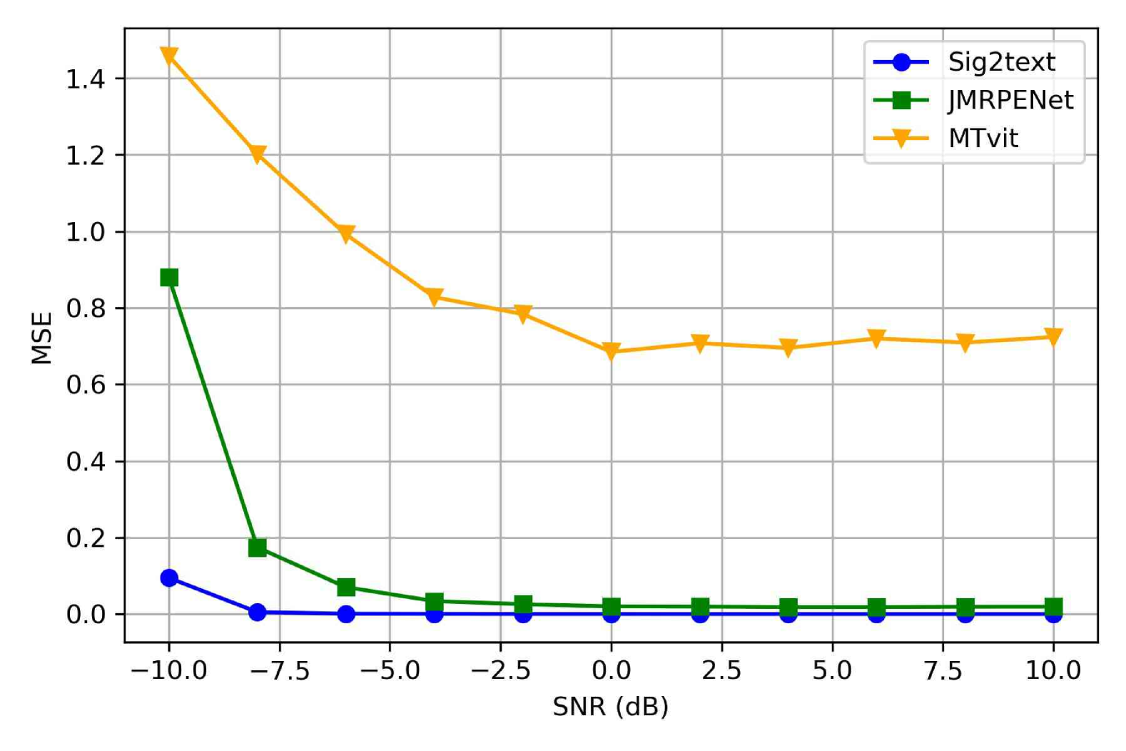
(a) cf

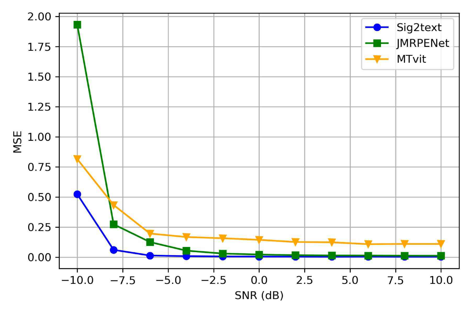
(b) B

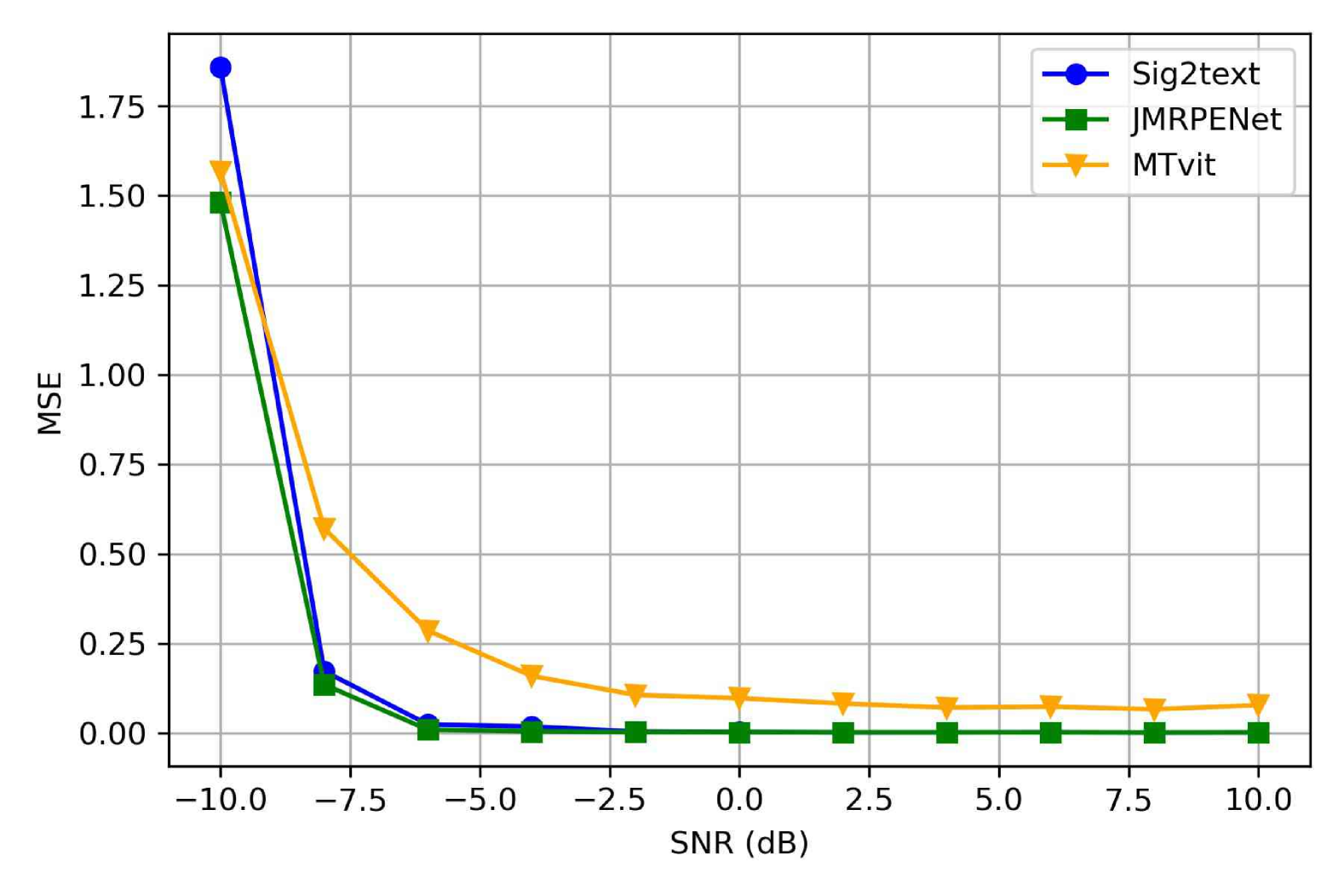
(c) T

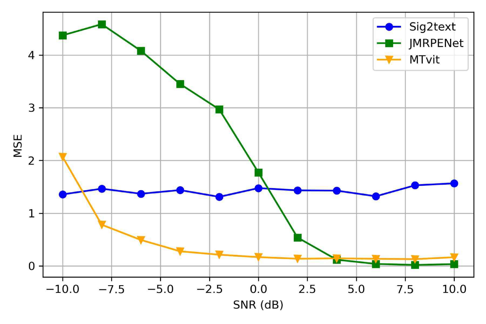
(d) segment_num

Figure 2: Parameters estimation performance for different method on different SNR levels

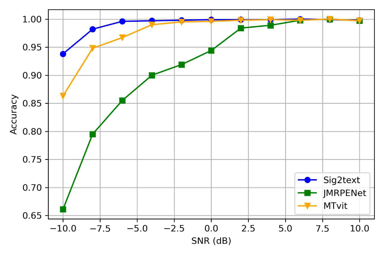
(a) Type Recognition Accuracy

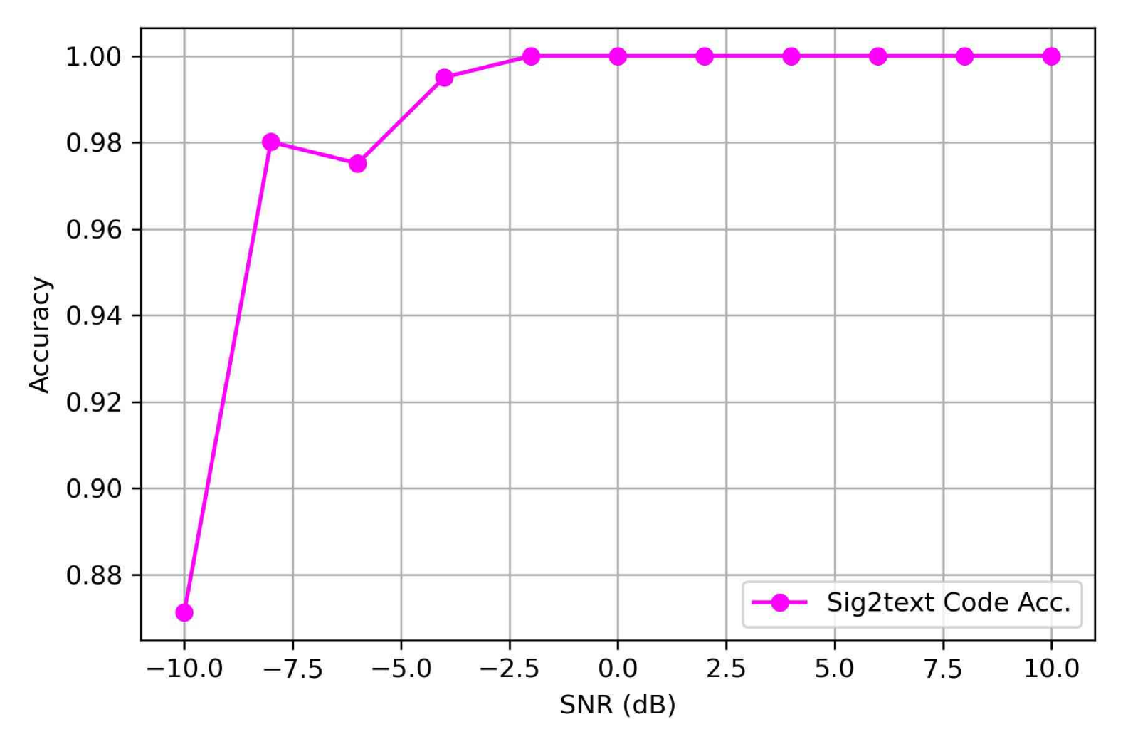
(b) Code Estimation Accuracy

Figure 3: Accuracy comparison and Sig2text Code Accuracy

5 Conclusion

In this paper, we propose Sig2text for radar signal recognition and parameter estimation. The method leverages the Vision Transformer architecture to extract time-frequency features from radar signals and uses a transformer-based decoder to parse the symbolic representation of the radar signals. The proposed method is evaluated on a synthetic radar signal dataset and compared with the baselines. The results show that Sig2text outperforms the baseline methods in both type recognition and parameter estimation tasks. The method is robust to noise and can achieve near-perfect performance even at low SNR levels.

References

- [1] Fatih Çağatay Akyön, Mustafa Atahan Nuhoğlu, Yaşar Kemal Alp, and Orhan Arıkan. Multi-Task Learning Based Joint Pulse Detection and Modulation Classification. In 2019 27th Signal Processing and Communications Applications Conference (SIU), pages 1–4, April 2019.
- [2] Canan Aydogdu, Musa Furkan Keskin, Gisela K Carvajal, Olof Eriksson, Hans Hellsten, Hans Herbertsson, Emil Nilsson, Mats Rydstrom, Karl Vanas, and Henk Wymeersch. Radar interference mitigation for automated driving: Exploring proactive strategies. IEEE Signal Processing Magazine, 37(4):72–84, 2020.
- [3] Guo Bai, Yufan Cheng, Wanbin Tang, and Shaoqian Li. Chirp Rate Estimation for LFM Signal by Multiple DPT and Weighted Combination. IEEE Signal Processing Letters, 26(1):149–153, January 2019.
- [4] Shannon D. Blunt and Eric L. Mokole. Overview of radar waveform diversity. IEEE Aerospace and Electronic Systems Magazine, 31(11):2–42, November 2016.
- [5] Kuiyu Chen, Lipo Wang, Jingyi Zhang, Si Chen, and Shuning Zhang. Semantic Learning for Analysis of Overlapping LPI Radar Signals. IEEE Transactions on Instrumentation and Measurement, 72:1–15, 2023.
- [6] Raja Kumari Chilukuri, Hari Kishore Kakarla, and K. Subbarao. Estimation of Modulation Parameters of LPI Radar Using Cyclostationary Method. Sensing and Imaging, 21(1):51, October 2020.
- [7] Freddy C Chua and Nigel P Duffy. DeepCPCFG: Deep learning and context free grammars for end-to-end information extraction. In International Conference on Document Analysis and Recognition, pages 838–853. Springer, 2021.
- [8] Alexey Dosovitskiy, Lucas Beyer, Alexander Kolesnikov, Dirk Weissenborn, Xiaohua Zhai, Thomas Unterthiner, Mostafa Dehghani, Matthias Minderer, Georg Heigold, Sylvain Gelly, et al. An image is worth 16x16 words: Transformers for image recognition at scale. arXiv preprint arXiv:2010.11929, 2020.
- [9] Zhiting Fei, Jiachen Zhao, Zhe Geng, Xiaohua Zhu, and Jindong Zhang. Hybrid FSK-PSK Waveform Optimization for Radar Based on Alternating Direction Method of Multiplier (ADMM). Sensors, 21(23):7915, January 2021.
- [10] Qiang Guo, Xin Yu, and Guoqing Ruan. LPI Radar Waveform Recognition Based on Deep Convolutional Neural Network Transfer Learning. Symmetry, 11(4):540, April 2019.
- [11] Yuanpu Guo, Haixin Sun, Hui Liu, and Zhenmiao Deng. Radar Signal Recognition Based on CNN With a Hybrid Attention Mechanism and Skip Feature Aggregation. IEEE Transactions on Instrumentation and Measurement, 73:1–13, 2024.
- [12] Sevgi Zubeyde Gurbuz, Hugh D. Griffiths, Alexander Charlish, Muralidhar Rangaswamy, Maria Sabrina Greco, and Kristine Bell. An Overview of Cognitive Radar: Past, Present, and Future. IEEE Aerospace and Electronic Systems Magazine, 34(12):6–18, December 2019.
- [13] Thien Huynh-The, Van-Sang Doan, Cam-Hao Hua, Quoc-Viet Pham, Toan-Van Nguyen, and Dong-Seong Kim. Accurate LPI Radar Waveform Recognition With CWD-TFA for Deep Convolutional Network. IEEE Wireless Communications Letters, 10(8):1638–1642, August 2021.
- [14] Zehuan Jing, Peng Li, Bin Wu, Shibo Yuan, and Yingchao Chen. An Adaptive Focal Loss Function Based on Transfer Learning for Few-Shot Radar Signal Intra-Pulse Modulation Classification. Remote Sensing, 14(8):1950, January 2022.
- [15] Ilya Loshchilov and Frank Hutter. Decoupled weight decay regularization. In International Conference on Learning Representations.
- [16] Jarmo Lunden and Visa Koivunen. Automatic Radar Waveform Recognition. IEEE Journal of Selected Topics in Signal Processing, 1(1):124–136, June 2007.
- [17] Dingyou Ma, Nir Shlezinger, Tianyao Huang, Yimin Liu, and Yonina C Eldar. Joint radar-communication strategies for autonomous vehicles: Combining two key automotive technologies. IEEE signal processing magazine, 37(4):85–97, 2020.
- [18] Jin Ming, Sheng xulong, and Hu Guobing. Intrapulse modulation recognition of radar signals based on statistical tests of the time-frequency curve. In Proceedings of 2011 International Conference on Electronics and Optoelectronics, volume 1, pages V1–300–V1–304, July 2011.
- [19] Phillip E. Pace. Detecting and Classifying Low Probability of Intercept Radar. Artech House Radar Library. Artech House, Boston, 2nd ed edition, 2009.
- [20] Zhiyu Qu, Wenyang Wang, Changbo Hou, and Chenfan Hou. Radar signal intra-pulse modulation recognition based on convolutional denoising autoencoder and deep convolutional neural network. IEEE Access, 7:112339–112347, 2019.
- [21] Jun Sun, Guangluan Xu, Wenjuan Ren, and Zhiyuan Yan. Radar emitter classification based on unidimensional convolutional neural network. IET Radar, Sonar & Navigation, 12(8):862–867, August 2018.
- [22] Wan Tao, Jiang Kaili, Liao Jingyi, Jia Tingting, and Tang Bin. Research on LPI radar signal detection and parameter estimation technology. Journal of Systems Engineering and Electronics, 32(3):566–572, June 2021.
- [23] Ashish Vaswani, Noam Shazeer, Niki Parmar, Jakob Uszkoreit, Llion Jones, Aidan N Gomez, Łukasz Kaiser, and Illia Polosukhin. Attention is All you Need. In Advances in Neural Information Processing Systems, volume 30. Curran Associates, Inc., 2017.
- [24] Nikita Visnevski, Vikram Krishnamurthy, Alex Wang, and Simon Haykin. Syntactic Modeling and Signal Processing of Multifunction Radars: A Stochastic Context-Free Grammar Approach. Proceedings of the IEEE, 95(5):1000–1025, May 2007.
- [25] Shunjun Wei, Qizhe Qu, Hao Su, Mou Wang, Jun Shi, and Xiaojun Hao. Intra-pulse modulation radar signal recognition based on CLDN network. IET Radar, Sonar & Navigation, 14(6):803–810, 2020.
- [26] Shibo Yuan, Bin Wu, and Peng Li. Intra-Pulse Modulation Classification of Radar Emitter Signals Based on a 1-D Selective Kernel Convolutional Neural Network. Remote Sensing, 13(14):2799, January 2021.
- [27] Deguo Zeng, Hui Xiong, Jun Wang, and Bin Tang. An Approach to Intra-Pulse Modulation Recognition Based on the Ambiguity Function. Circuits, Systems and Signal Processing, 29(6):1103–1122, December 2010.
- [28] Jingyi Zhang, Jiaxing Huang, Sheng Jin, and Shijian Lu. Vision-Language Models for Vision Tasks: A Survey. IEEE Transactions on Pattern Analysis and Machine Intelligence, 46(8):5625–5644, August 2024.
- [29] Yuefeng Zhao, Shengliang Han, Jimin Yang, Liren Zhang, Huaqiang Xu, and Jingjing Wang. A Novel Approach of Slope Detection Combined with Lv’s Distribution for Airborne SAR Imagery of Fast Moving Targets. Remote Sensing, 10(5):764, May 2018.
- [30] Mengtao Zhu, Ziwei Zhang, Cong Li, and Yunjie Li. JMRPE-Net: Joint modulation recognition and parameter estimation of cognitive radar signals with a deep multitask network. IET Radar, Sonar & Navigation, 15(11):1508–1524, 2021.
- [31] Ming Zhu, Wei-Dong Jin, Yun-Wei Pu, and Lai-Zhao Hu. Classification of radar emitter signals based on the feature of time-frequency atoms. In 2007 International Conference on Wavelet Analysis and Pattern Recognition, volume 3, pages 1232–1236, November 2007.
- [32] Bahman Zohuri. Radar Energy Warfare and the Challenges of Stealth Technology. Springer, 2020.