Constraining Axially Symmetric Bianchi Type I Model with Self-Consistent Recombination History and Observables

Abstract

Recent cosmological measurements suggest the possibility of an anisotropic universe. As a result, the Bianchi Type I model, being the simplest anisotropic extension to the standard Friedmann–Lemaître–Robertson–Walker metric has been extensively studied. In this work, we show how the recombination history should be modified in an anisotropic universe and derive observables by considering the null geodesic. We then constrain the axially symmetric Bianchi Type I model by performing Markov Chain Monte Carlo with the acoustic scales in Cosmic Microwave Background (CMB) and Baryon Acoustic Oscillation data, together with local measurements of $H(z)$ and Pantheon Supernova data. Our results reveal that the anisotropic model is not worth a bare mention compared to the $\Lambda$CDM model, and we obtain a tight constraint on the anisotropy that generally agrees with previous studies under a maximum temperature anisotropy fraction of $2\text{\times}{10}^{-5}$. To allow for a non-kinematic CMB dipole, we also present constraints based on a relaxed maximum temperature anisotropy comparable to that of the CMB dipole. We stress that there is a significant difference between the geodesic-based observables and the naive isotropic analogies when there is a noticeable anisotropy. However, the changes in recombination history are insignificant even under the relaxed anisotropy limit.

I Introduction

The Cosmological Principle (CP) of homogeneity and isotropy on large scales is a foundational assumption in the standard $\Lambda$CDM cosmological model with the flat Friedmann–Lemaître–Robertson–Walker (FLRW) metric

$$ds^{2}=-dt^{2}+\mathfrak{a}^{2}(t)\left(dx^{2}+dy^{2}+dz^{2}\right),$$ (1)

where $\mathfrak{a}$ is the usual scale factor. However, recent analyses of cosmological measurements at both large and local scales challenge this assumption.

Global measurements, such as those of the Cosmic Microwave Background (CMB), have long been suspected to exhibit large-scale anisotropies. Even back in the Wilkinson Microwave Anisotropy Probe (WMAP) data, anomalies that hint at a large-scale spatial anisotropy emerge, such as the alignment of the quadrupole and octopole axes [1, 2, 3, 4], the North-South asymmetry [5, 6, 7, 8], and hints of some preferred axes [9, 5, 6, 10, 11]. Furthermore, several cosmological parameters ($n_{s}$, $A_{s}$, and $\Omega_{b0}$) exhibit anisotropic distributions across the full sky [12].

Such anomalies did not disappear with the more precise data from Planck. Instead, more and more evidence suggests the existence of large-scale anisotropy. An example is the CMB parity asymmetry which has a preferred axis roughly aligning the CMB dipole, quadrupole, and octopole [13, 14, 15, 16]. In addition, all six cosmological parameters $\set{\Omega_{b}h^{2},\Omega_{c}h^{2},n_{s},100\theta_{\mathrm{MC}},\tau,\ln{(10^{10}A_{s})}}$, in addition to the Hubble constant $H_{0}$, are found to exhibit a dipole distribution at 2-3$\sigma$ level, with generally aligned dipole directions [17]. Hence, both the Wilkinson Microwave Anisotropy Probe (WMAP) and Planck data indicate an anisotropic universe, contradicting the assumed CP.

Interestingly, several local measurements also show anisotropic features. In particular, the bulk flow of galaxies [18, 19] and the quasar polarization [20] have been observed to align with the CMB dipole. Various Type Ia Supernova (SNIa) measurements [21, 22, 23, 24, 25] also suggest directional dependency in cosmic acceleration and $H_{0}$, with a generally larger value near the CMB dipole direction [22, 23, 24, 25]. However, the directions of the preferred axes vary in different studies. For a detailed review, see Ref. [21, 26, 27].

These observations suggest that either significant unknown systematics pollute both the CMB and local measurements or CP is indeed inexact. We are thus motivated to consider a Bianchi Type I model

$$ds^{2}=-dt^{2}+a^{2}(t)dx^{2}+b^{2}(t)dy^{2}+c^{2}(t)dz^{2}$$ (2)

which is anisotropic but homogeneous and is a natural anisotropic extension of the FLRW metric [28, 29, 30, 31, 32]. Here, $a(t)$, $b(t)$, and $c(t)$ are the scale factors in the $x$, $y$ and $z$ directions, respectively, which may be distinct from the FLRW scale factor $\mathfrak{a}$. To reduce the number of parameters, we consider a subset of the Bianchi Type I model, the axially symmetric model, where $a(t)=b(t)$, though our method can be extended to the general Bianchi Type I model.

There have been attempts to constrain the extent of anisotropy of a Bianchi Type I universe using global and local cosmological data [28, 29, 30, 33, 31, 34]. The authors of Ref. [28, 30, 33, 31] considered the evolution of the geometric mean of the scale factors $a,\ b$ and $c$ by a modified Friedmann equation and observables constructed from the mean scale factors. Besides, some authors would fix the physical baryon density to the $\Lambda$CDM value [28, 33]. Meanwhile, although Ref. [32] did not adopt such definitions of observables, only order-of-magnitude constraints were derived at the fixed decoupling time $t_{\mathrm{CMB}}\sim$0.38\text{\,}\mathrm{Myr}$$, based on the CMB temperature anisotropy or at the fixed time of Big Bang nucleosynthesis (BBN). These prompt us to re-constrain an axially symmetric Bianchi Type I model with self-consistently defined recombination history, distances, and hence observables.

In Sec. II, we first introduce the anisotropic universe model considered. In particular, the expansion equations and corresponding thermodynamics history are discussed. Subsequently, we review the definitions of observables adopted by previous works in Sec. III and present how comoving distances, observables and their full-sky averages should be defined. Next, we discuss how we constrain the anisotropic cosmological parameters (Sec. IV). The results are presented and discussed in Sec. V. Finally, in Sec. VI, we conclude.

II The Anisotropic universe

II.1 Axially Symmetric Bianchi Type I Model

In the Bianchi Type I model, the line element in the matter-comoving coordinate (4-velocity $u^{\mu}=\delta^{\mu}_{0}$) is given by Eq. 2 [28, 33, 32, 30, 34]. Note that the corresponding scale factors for the 3 directions $\set{a(t),b(t),c(t)}$ are generally different, implying an anisotropic universe. Subsequently, the Hubble parameters in the 3 directions are defined as

$$H_{x} =\frac{\dot{a}}{a}, H_{y} =\frac{\dot{b}}{b}, H_{z} =\frac{\dot{c}}{c}.$$ (3)

The dot here denotes a derivative with respect to time.

On the other hand, the energy-momentum tensor $T\indices{{}^{\mu}_{\nu}}$, including radiation ($r$), matter ($m$), and dark energy (in the form of the cosmological constant $\Lambda$) takes the form

$$T\indices{{}^{\mu}_{\nu}} =\text{diag}(-\rho,p_{x},p_{y},p_{z}),$$ (4)

$$=\text{diag}(-\rho,p,p,p)$$

where $\rho=\sum\rho_{X}=\rho_{r}+\rho_{m}+\rho_{\Lambda}$ and $p=\sum p_{X}=p_{r}+p_{m}+p_{\Lambda}$ are, respectively, the total energy density and the total pressure. Note that the assumption of isotropic pressure is applied in the second line [28, 30, 33, 29, 32] and radiation includes contribution from massless neutrinos. Applying the local conservation law

$$\nabla_{\mu}T\indices{{}^{\mu\nu}}=0$$ (5)

to the energy-momentum tensor gives the time evolution equation

$$\dot{\rho}_{X}+(1+w_{X})\rho_{X}(H_{x}+H_{y}+H_{z}) =0,$$ (6)

with $p_{X}=w_{X}\rho_{X}$. Here, the equation of state (EOS) parameters $(w_{r},w_{m},w_{\Lambda})$ equal to $(1/3,0,-1)$. To study how energy densities vary with the scale factors, Eq. 6 can be solved analytically

$$\rho_{X}=\rho_{X0}\left(\frac{abc}{a_{0}b_{0}c_{0}}\right)^{-(1+w_{X})}.$$ (7)

The subscript ‘0’ denotes the current-day value throughout this work. The energy densities scale just like under the FLRW metric but with $\mathfrak{a}^{3}$ replaced by $(abc)$.

The expansion history is given by solving the Einstein Field Equation

$$G\indices{{}_{\mu\nu}}=8\pi T\indices{{}_{\mu\nu}},$$ (8)

which contains 4 non-trivial equations

$$H_{x}H_{y}+H_{y}H_{z}+H_{z}H_{x}=8\pi\rho,$$ (9)

$$\frac{\ddot{b}}{b}+H_{y}H_{z}+\frac{\ddot{c}}{c}=-8\pi p,$$ (10)

$$\frac{\ddot{c}}{c}+H_{z}H_{x}+\frac{\ddot{a}}{a}=-8\pi p,$$ (11)

$$\frac{\ddot{a}}{a}+H_{x}H_{y}+\frac{\ddot{b}}{b}=-8\pi p.$$ (12)

Now, we restrict ourselves to an axially symmetric model $(a=b)$ [32, 31] and examine Eqs. 10, 11 and 12, which reduce to

$$\ddot{a}=-a\left(4\pi p+\frac{1}{2}H_{x}^{2}\right),$$ (13)

$$\ddot{c}=-c\left(8\pi p+H_{x}H_{z}+\frac{\ddot{a}}{a}\right).$$ (14)

Combining Eqs. 13 and 14 with the axially symmetric version of Eq. 6

$$\dot{\rho}_{X}+(1+w_{X})\rho_{X}(2H_{x}+H_{z})=0,$$ (15)

one can solve the time evolution of the universe by providing the initial conditions $(H_{x0},H_{z0},\rho_{m0},\rho_{r0},\rho_{\Lambda 0})$. In particular, the current values of the scale factors are set to one, i.e., $a_{0}=c_{0}=1$ since the line element in Eq. 2 is invariant if $a\rightarrow\lambda a,\ dx\rightarrow dx/\lambda$ and similarly for $c$. Lastly, it is important to emphasize that we are considering a flat universe, $\rho_{r0}+\rho_{m0}+\rho_{\Lambda 0}=\rho_{\text{crit0}}$, the critical density of the universe. Hence, we only have 2 energy densities as model parameters. From Eq. 9, the flatness criterion implies [35]

$$\rho_{r0}+\rho_{m0}+\rho_{\Lambda 0}=\rho_{\text{crit}0}=\frac{H_{x0}^{2}+2H_{x0}H_{z0}}{8\pi}.$$ (16)

II.2 Thermodynamics of the Anisotropic Universe

One needs to consider the thermodynamics of the universe to track the recombination history. This work assumes thermal equilibrium from the beginning of time till the last scattering of CMB photons, justified by the rapid interactions. After the last scattering, photons propagate freely while maintaining the shape of a blackbody spectrum. Under the Bianchi Type I model, photons traveling in different directions experience different cosmological redshifts due to the directional-dependent scale factor. Hence, the temperature and the blackbody spectrum would have a directional dependency. However, by enforcing that the CMB temperature anisotropies at present-day are of the order of ${10}^{-5}$ [36], the directional dependency of temperature is negligible, and an isotropic temperature is a good approximation. Furthermore, we stress that the anisotropy exists only at the metric level, manifesting through the scale factors. Hence, the usual thermodynamics equations are valid with suitable modifications related to the scale factors. For instance, by considering radiation with $\rho_{r}\propto T^{4}$ (from statistical mechanics) and $\rho_{r}\propto(abc)^{-4/3}$ [from Eq. 7], we obtain

$$T\propto(abc)^{-1/3},$$ (17)

analogous to that under the FLRW metric.

The thermodynamics are crucial in finding the moment of the last scattering. There are well-developed thermodynamics codes such as HyRec [37, 38] that calculate the recombination process by keeping track of complicated atomic transitions. However, they use the FLRW scale factor $\mathfrak{a}$ as the temporal coordinate and thus cannot be easily modified for our model. Instead, we consider the contribution from Hydrogen only and follow Peebles’ formalism [39, 40, 41] to approximate the electron fraction $X_{e}$ evolution and the recombination history. This approach also offers the advantage of providing a more analytical understanding of how the recombination history is influenced by anisotropy. Most factors in the Peebles’ formalism are independent of the expansion of the universe, so we need not change anything except for $\Lambda_{\alpha}$, which is the rate of recombination via resonance escape [40]. Under the usual FLRW metric,

$$\Lambda_{\alpha}=\frac{27}{128\zeta(3)}\frac{\mathfrak{H}(t)}{[1-X_{e}(t)]\eta[k_{B}T(t)/E_{I}]^{3}},$$ (18)

where $\eta$ is the baryon-to-photon ratio, $k_{B}$ is the Boltzmann constant, and $E_{I}$ is the ionization energy of Hydrogen. Here, $\mathfrak{H}$ is the Hubble parameter under the FLRW metric that describes the cosmological redshift of photons and thus needs to be modified [40, 41]. Suppose a photon is emitted in a FLRW universe at $t=t_{e}$ and is measured at $t=t^{\prime}$, the photon frequency is redshifted by

$$\frac{\left.\mathfrak{a}\right\rvert_{t_{e}}}{\left.\mathfrak{a}\right\rvert_{t^{\prime}}}.$$ (19)

By Taylor expanding near $t^{\prime}=t_{e}$, we have

$$\frac{\left.\mathfrak{a}\right\rvert_{t_{e}}}{\left.\mathfrak{a}\right\rvert_{t^{\prime}}}=1-\left.\frac{\dot{\mathfrak{a}}}{\mathfrak{a}}\right\rvert_{t_{e}}(t^{\prime}-t_{e})=1-\mathfrak{H}(t_{e})(t^{\prime}-t_{e}).$$ (20)

For an axially symmetric Bianchi Type I metric, the photon frequency is redshifted by

$$\frac{\left.(a^{2}c)^{1/3}\right\rvert_{t_{e}}}{\left.(a^{2}c)^{1/3}\right\rvert_{t^{\prime}}}.$$ (21)

Expanding around $t^{\prime}=t_{e}$, we obtain

$$\frac{\left.(a^{2}c)^{1/3}\right\rvert_{t_{e}}}{\left.(a^{2}c)^{1/3}\right\rvert_{t^{\prime}}}=1-\frac{1}{3}\left[2\frac{\dot{a}}{a}+\frac{\dot{c}}{c}\right]_{t_{e}}(t^{\prime}-t_{e}).$$ (22)

Therefore, by replacing

$$\mathfrak{H}\to\frac{1}{3}\left(2\frac{\dot{a}}{a}+\frac{\dot{c}}{c}\right),$$ (23)

one obtains the resonance escape rate $\Lambda_{\alpha}$ under the axially symmetric universe and by extension, the $X_{e}$ evolution.

Consequently, we are equipped to find the optical depths by ignoring the contribution from reionization. Following the definition of Planck [42, 43, 36], we denote the time when the photon optical depth

$$\tau=\int_{t_{*}}^{t_{0}}\sigma_{T}n_{b}X_{e}dt$$ (24)

and the time when the baryon-drag optical depth

$$\tau_{\mathrm{drag}}=\int_{t_{\mathrm{drag}}}^{t_{0}}R\sigma_{T}n_{b}X_{e}dt$$ (25)

equal to unity by $t_{*}$ and $t_{\mathrm{drag}}$, respectively. Note that $\sigma_{T}$ is the Thomson cross-section, $n_{b}$ is the baryon number density and $R=[3\rho_{b}(t)]/[4\rho_{r}(t)]$.

III Distance and Observables

III.1 Comments on Previous Definitions

Ref. [28, 30, 33] solved the expansion history of a Bianchi Type I universe by considering the evolution of the geometric mean of the directional scale factors

$$\tilde{a}=\sqrt[3]{abc},$$ (26)

$$1+\tilde{z}=\frac{1}{\tilde{a}},$$ (27)

$$\tilde{H}=\frac{\dot{\tilde{a}}}{\tilde{a}}=\frac{1}{3}(H_{x}+H_{y}+H_{z}).$$ (28)

From this, they derived the corresponding first Friedmann equation [28, 30, 33]

$$\tilde{H}(\tilde{a})^{2}=\tilde{H}_{0}^{2}\left(\tilde{\Omega}_{r0}\tilde{a}^{-4}+\tilde{\Omega}_{m0}\tilde{a}^{-3}+\tilde{\Omega}_{\Lambda 0}+\tilde{\Omega}_{\sigma 0}\tilde{a}^{-6}\right),$$ (29)

where $\tilde{\Omega}_{X0}$ here is the dimensionless energy density defined using $\tilde{H}$ instead of the $\Lambda$CDM $\mathfrak{H}$. Moreover, there is an additional energy density $\tilde{\Omega}_{\sigma 0}=\sigma^{2}/(3\tilde{H}^{2})$ generated by the shear scalar $\sigma^{2}$ [28, 30, 33]. The above is equivalent to the previous treatment in section II.1 and can even be applied in section II.2. The authors obtained a neat modified Friedmann equation in exchange for information on individual scale factors $a$, $b$, and $c$.

However, inconsistency arises when the authors try to define observables in the same manner as they would within the $\Lambda$CDM framework. For instance, the authors [28, 33] define the comoving sound horizon at drag redshift $\tilde{z}_{d}$ as

$$\tilde{r}_{s}=\int_{\tilde{z}_{d}}^{\infty}\frac{c_{s}d\tilde{z}}{\tilde{H}(\tilde{z})},$$ (30)

in the same way as in the FLRW metric. Obviously, the sound horizon $\tilde{r}_{s}$ lacks directional dependency, a major characteristic of any anisotropic model. Hence, such observables constructed by drawing parallels between the Bianchi Type I and the FLRW metrics are not appropriate. Indeed, the geometric mean of the scale factors $\tilde{a}$ only serves as a convenient tool to solve for the dynamics of the Bianchi Type I universe, but it should not be used in defining observables.

III.2 Comoving Distance

The comoving distance is defined as the distance between two points in comoving coordinates [44]

$$dD_{C}^{2}=dx^{2}+dy^{2}+dz^{2}.$$ (31)

Now, consider a null geodesic [44]

$$1=a^{2}\left(\frac{dx}{dt}\right)^{2}+b^{2}\left(\frac{dy}{dt}\right)^{2}+c^{2}\left(\frac{dz}{dt}\right)^{2},$$ (32)

connecting the observer who is, without loss of generality, positioned at the origin, and the source which is positioned at a polar angle $\Theta$ and an azimuthal angle $\phi$ such that

$$\frac{dy}{dx}=\tan\phi,$$ (33)

$$\frac{d\ell}{dz}=\tan\Theta,$$ (34)

$$d\ell^{2}=dx^{2}+dy^{2}.$$ (35)

Thus, in agreement with Ref. [34],

$$D_{C}(\Theta,\phi,t_{1},t_{2})=\int_{t_{1}}^{t_{2}}\frac{dt}{\sqrt{\xi^{2}\sin^{2}\Theta+c^{2}\cos^{2}\Theta}},$$ (36)

$$\xi^{2}=a^{2}\cos^{2}\phi+b^{2}\sin^{2}\phi.$$ (37)

For an axially symmetric universe ($a=b$), Eq. 36 is simplified to

$$D_{C}(\Theta,t_{1},t_{2})=\int_{t_{1}}^{t_{2}}\frac{dt}{\sqrt{a^{2}\sin^{2}\Theta+c^{2}\cos^{2}\Theta}}.$$ (38)

An effective scale factor can thus be defined

$$a_{\mathrm{eff}}(\Theta,t)=\sqrt{a(t)^{2}\sin^{2}\Theta+c(t)^{2}\cos^{2}\Theta},$$ (39)

such that

$$D_{C}(\Theta,t_{1},t_{2})=\int_{t_{1}}^{t_{2}}\frac{dt}{a_{\mathrm{eff}}},$$ (40)

resembling the comoving distance in the FLRW metric, but now with explicit directional dependency.

III.3 Observables

Observables like angular acoustic scales in CMB and Baryon Acoustic Oscillation (BAO) as well as Supernova distance moduli are derived from more fundamental quantities such as the transverse comoving diameter distance. In the following, we discuss how the observables are defined under the axially symmetric model.

III.3.1 Directional Hubble Parameter

The effective scale factor at the polar angle $\Theta$ and time $t_{\mathrm{obs}}$ is defined in Eq. 39. Consequently, one can construct the corresponding Hubble parameter

$$H(\Theta,t_{\mathrm{obs}}) =\frac{1}{a_{\mathrm{eff}}(\Theta,t_{\mathrm{obs}})}\frac{da_{\mathrm{eff}}}{dt}$$ (41)

$$=\frac{a\dot{a}\sin(\Theta)^{2}+c\dot{c}\cos(\Theta)^{2}}{a^{2}\sin(\Theta)^{2}+c^{2}\cos(\Theta)^{2}}.$$

III.3.2 Comoving Sound Horizon

Considering a general last scattering time $t_{\mathrm{ls}}$, we derive the equation for the comoving sound horizon $r_{\mathrm{ls}}$. At $t_{\mathrm{ls}}$, the sound waves would have propagated out to an ellipsoidal surface. According to Eq. 38, its semi-axes along the principal directions are

$$\begin{aligned} L_{x,y}&=\int_{0}^{t_{\mathrm{ls}}}\frac{c_{s}(t)dt}{a(t)},&&\text{for $x$ and $y$-direction},\\ L_{z}&=\int_{0}^{t_{\mathrm{ls}}}\frac{c_{s}(t)dt}{c(t)},&&\text{for $z$ direction},\end{aligned}$$ (42)

$$c_{s}(t)=\frac{1}{\sqrt{3(1+R(t))}}.$$ (43)

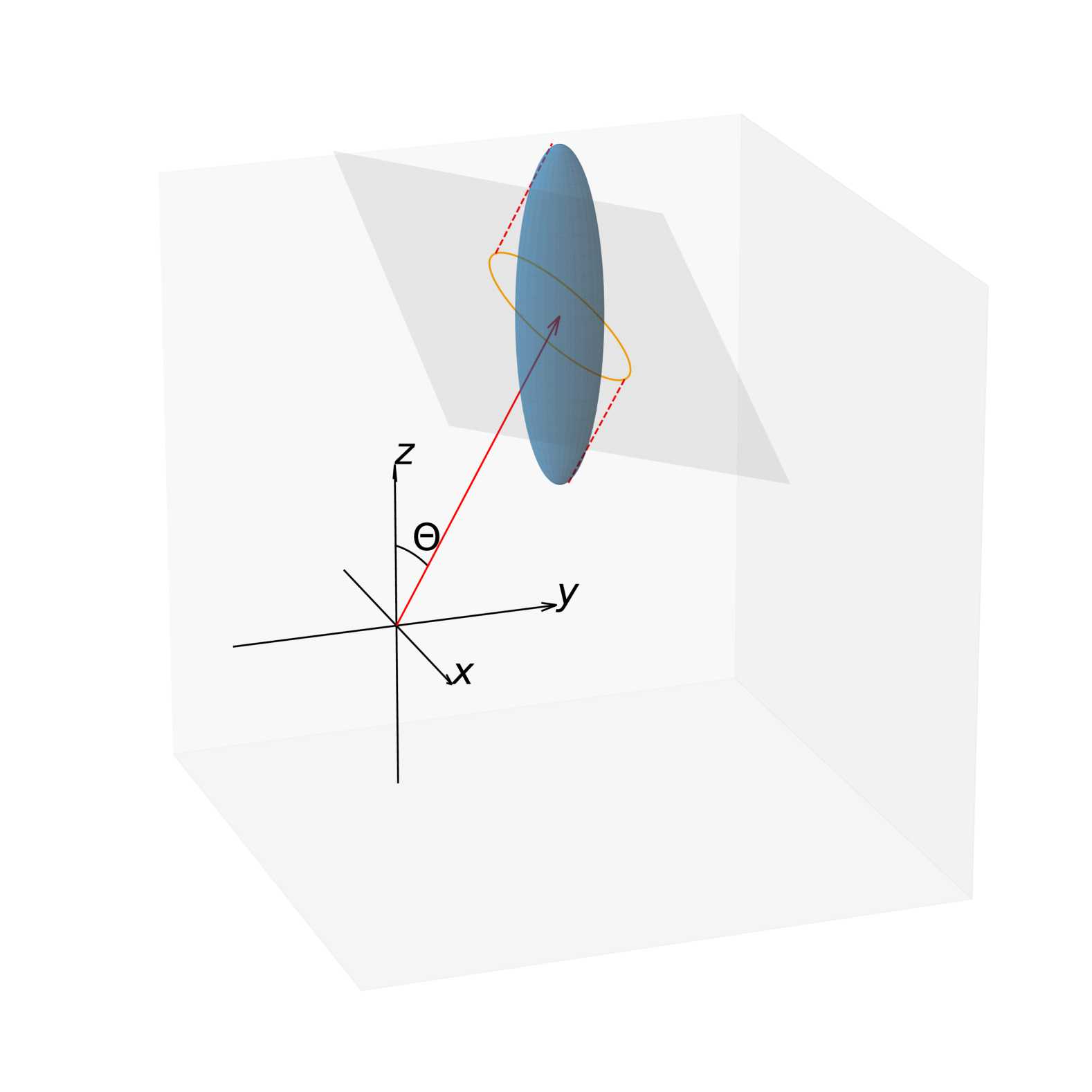
Figure 1: Schematic of the sound horizon at a polar angle $\Theta$. The sound waves form an ellipsoidal surface (the blue surface) and the observer at the origin would observe an ellipse (the orange line) as the projection along the radial direction.

The maximum region of correlation observed at a polar angle $\Theta$ is defined by the projection of the ellipsoid along the radial direction, as indicated by the orange ellipse in Fig. 1. By geometry, an observer at the origin observes an ellipse with semi-axes

$$\tilde{L}_{1}=L_{x,y},$$ (44)

$$\tilde{L}_{2}=\sqrt{L_{x,y}^{2}\cos^{2}\Theta+L_{z}^{2}\sin^{2}\Theta}.$$ (45)

Note that due to the symmetry in the $x$ and $y$-axes, $\tilde{L}_{1}=L_{x,y}$. We consider the area of the ellipse and define an effective comoving sound horizon by

$$r_{\mathrm{ls}}(\Theta,t_{\rm ls})=\sqrt{\frac{\rm{Area}(\Theta,t_{\rm ls})}{\pi}},$$ (46)

$$\mathrm{Area}=\pi\tilde{L}_{1}\tilde{L}_{2}=\pi L_{x,y}\sqrt{L_{x,y}^{2}\cos^{2}\Theta+L_{z}^{2}\sin^{2}\Theta}.$$ (47)

III.3.3 Angular Scales and Inverse Angular Scales

The CMB angular acoustic scale at angle $\Theta$ is defined as the ratio of the sound horizon $r_{*}$ and the transverse comoving diameter distance $D_{M,*}$:

$$\theta_{*}(\Theta)=\frac{r_{*}}{D_{M,*}(\Theta)},$$ (48)

$$r_{*}(\Theta)=r_{\mathrm{ls}}(\Theta,t_{*}),$$ (49)

$$D_{M,*}(\Theta)=D_{C}(\Theta,t_{*},t_{0}).$$ (50)

The BAO observables are defined similarly. For objects at time $t_{\mathrm{obs}}$, we follow the definition of DESI [45] and define the BAO-related distances as

$$r_{d}(\Theta)=r_{\mathrm{ls}}(\Theta,t_{d}),$$ (51)

$$D_{M,d}(\Theta,t_{\mathrm{obs}})=D_{C}(\Theta,t_{\mathrm{obs}},t_{0}),$$ (52)

$$D_{A,d}(\Theta,t_{\mathrm{obs}})=a_{\mathrm{eff}}(\Theta,t_{\mathrm{obs}})D_{M,d}(\Theta,t_{\mathrm{obs}}),$$ (53)

$$D_{H,d}(\Theta,t_{\mathrm{obs}})=\frac{1}{H(\Theta,t_{\mathrm{obs}})},$$ (54)

$$D_{V,d}(\Theta,t_{\mathrm{obs}})=\left(D_{M,d}^{2}\frac{1}{a_{\mathrm{eff}}+1}D_{V,d}\right)^{1/3}.$$ (55)

From Eqs. 51, 52, 53, 54 and 55, we can construct the (inverse) angular acoustic scales $D_{M,d}/r_{d}$, $D_{A,d}/r_{d}$, $D_{H,d}/r_{d}$, $D_{V,d}/r_{d}$, $Hr_{d}$ and $r_{d}/D_{V,d}$.

III.3.4 Type Ia Supernova Luminosity Distance

In $\Lambda$CDM, the luminosity distance of a Supernova at the heliocentric redshift $z_{\text{helio}}$ and the CMB rest frame redshift $z_{\text{CMB}}$ is [28]

$$d_{L} =(1+z_{\text{helio}})\int_{0}^{z_{\text{CMB}}}\frac{dz}{H(z)}$$ (56)

$$=(1+z_{\text{helio}})\cdot\text{ Comoving Distance to }z_{\text{CMB}}.$$

Extending this to the anisotropic universe is straightforward, by replacing the FLRW comoving distance by $D_{C}$ defined in Eq. 38.

IV Methodology and Data

IV.1 Methodology

We numerically solve the thermodynamics evolution and the expansion of the universe using the LSODA method [46, 47]. Notably, we use the Saha equation to solve for the electron fraction $X_{e}$ at the early times. Once the temperature cools to $6500\text{\,}\mathrm{K}$, we solve for $X_{e}(t)$, and thus, $t_{*}$ and $t_{d}$ by using the modified Peebles’ formalism outlined in section II.2. To account for the approximation in Peebles’ formalism and possible numerics, a small correction factor is introduced to $t_{*}$ and $t_{d}$ based on a comparison with the standard cosmological code CLASS [48] alongside the recombination code HyRec [37, 38]. We also check for the accuracy of our code by comparing it with CLASS [48] under the standard $\Lambda$CDM setting. The discrepancies in both the photon last scattering redshift and $100\theta_{*}$ are within the Planck error bars, indicating good agreement.

To search for suitable anisotropic cosmological parameters, we make use of the Monte Carlo code Cobaya [49, 50] with the built-in Markov Chain Monte Carlo (MCMC) sampler [51, 52]. A convergence threshold of Gelman-Rubin statistics quantity $R-1<0.01$ is chosen. We consider the parameter space $\{H_{x0},\omega_{b0},\omega_{c0},\alpha\}$, where

$$\alpha\equiv\frac{H_{z0}}{H_{x0}}-1,$$ (57)

and the physical densities

$$\omega_{b0}\equiv\frac{8\pi\rho_{b0}}{3}\xrightarrow{\text{\acs{FLRW}}}\Omega_{b}h^{2},$$ (58)

$$\omega_{c0}\equiv\frac{8\pi\rho_{c0}}{3}\xrightarrow{\text{\acs{FLRW}}}\Omega_{c}h^{2},$$ (59)

carrying similar meaning as $\Omega_{b}h^{2}$ and $\Omega_{c}h^{2}$ under the FLRW metric, respectively. The priors are summarized in Table 1. In particular, only a relatively small $|\alpha|<${10}^{-9}$$ is considered since we require the present-day CMB temperature anisotropies $\delta T/T\equiv|T_{x0}-T_{z0}|/$2.7255\text{\,}\mathrm{K}$<$2\text{\times}{10}^{-5}$$ with

$$T_{x0}=T(t_{*})\cdot\frac{a(t_{*})}{a_{0}}, T_{z0}=T(t_{*})\cdot\frac{c(t_{*})}{c_{0}}.$$ (60)

Moreover, since $\alpha$ can be positive or negative, corresponding to whether the $z$-axis is expanding faster than the $x$ and $y$-axes or not, we consider 2 different choices of the prior for $\alpha$, referred to as Prior A and B, respectively.

Due to the alignment of the CMB dipole, quadrupole and octopole [13, 14, 15, 16], it is natural to question the validity of the pure kinematic origin of the CMB dipole. Hence, we are motivated to consider the case that the intrinsic anisotropy of the universe contributes to a significant proportion of the observed CMB dipole, that is, we relax the constraint on temperature anisotropy to $\delta T/T<${10}^{-3}$$. Therefore, we consider 2 additional sets of prior, Prior C and D with a wider range for $\alpha$. Finally, the results are analyzed using the Python package GetDist [53] and a modified version of MCEvidence [54], specifically adapted for Cobaya chains.

		$\delta T/T<$2\text{\times}{10}^{-5}$$		$\delta T/T<${10}^{-3}$$
Parameter	$\Lambda$CDM	Prior A	Prior B	Prior C	Prior D
$H_{x0}$	$\mathcal{U}$($60$, $75$)	$\mathcal{U}$($60$, $80$)	$\mathcal{U}$($60$, $80$)	$\mathcal{U}$($60$, $80$)	$\mathcal{U}$($60$, $80$)
$\omega_{b0}$	$\mathcal{U}$($0.005$, $0.1$)	$\mathcal{U}$($0.005$, $0.030$)	$\mathcal{U}$($0.005$, $0.030$)	$\mathcal{U}$($0.005$, $0.030$)	$\mathcal{U}$($0.005$, $0.030$)
$\alpha$	0	$\mathcal{U}$($-1\text{\times}{10}^{-9}$, $0$)	$\mathcal{U}$($0$, $1\text{\times}{10}^{-9}$)	$\mathcal{U}$($-3\text{\times}{10}^{-8}$, $0$)	$\mathcal{U}$($0$, $3\text{\times}{10}^{-8}$)

Table 1: The priors used in this work. The four sets of anisotropic priors considered are referred to as A, B, C, and D. For $\omega_{c0}$, all prior sets use $\mathcal{U}$($0.001$, $0.99$). Here, $\mathcal{U}(x_{1},x_{2})$ refers to a uniform distribution over the interval $x_{1}$ to $x_{2}$.

IV.2 Data

Due to the rapid isotropization [55, 28, 32], only the measurements involving early time quantities have decent constraining power on the anisotropy. Hence, we are motivated to consider observations of the CMB angular acoustic scale and the BAO (inverse) angular acoustic scales. To supplement and to better constrain the standard cosmological parameters, $H(z)$ measurements from cosmic chronometer, Lyman-alpha, and BAO, as well as magnitude measurements from SNeIa are employed.

Since CMB and BAO measurements already cover a large portion of the sky, full-sky averaged quantities approximate the actual observations well. The definition of full-sky observables is

$$\langle\mathrm{Observable}\rangle=\frac{1}{2}\int_{0}^{\pi}(\mathrm{Observable})\sin\Theta d\Theta.$$ (61)

In contrast, Hubble parameter measurements and SNIa measurements are often based on well-localized observations. Thus, it seems that we should consider their position information which would introduce three additional Euler angles to describe the orientation of the anisotropic axes relative to our astronomical coordinate system. However, owing to the rapid isotropization [55, 28, 32], at late times, when Supernova and Hubble parameter measurements are based, $a_{\mathrm{eff}}\approx a\approx c$ within ${10}^{-8}$ levels. Therefore, there is virtually no anisotropy in these local observables, meaning that treating these observables as full-sky averaged quantities is a reasonable approximation, and it has the advantage of reducing the number of parameters by three. Explicitly, this work considers the averaged quantities $\langle H\rangle$ and $\langle d_{L}\rangle$ for Hubble parameter and SNIa measurements, respectively.

In addition, we must develop a conversion between redshift and cosmological time since measurements are often given in redshift while our model is a function of cosmological time. For a given redshift $z_{\mathrm{obs}}$, the corresponding time $t_{\mathrm{obs}}$ should satisfy

$$1+z_{\mathrm{obs}}=\frac{1}{\langle a_{\mathrm{eff}}\rangle(t_{\mathrm{obs}})},$$ (62)

where

$$\langle a_{\mathrm{eff}}\rangle(t_{\mathrm{obs}})=\frac{1}{2}\int_{0}^{\pi}a_{\mathrm{eff}}(\Theta,t_{\mathrm{obs}})\sin\Theta d\Theta,$$ (63)

is the full-sky averaged scale factor.

IV.2.1 CMB Angular Acoustic Scale

Planck 2018 gives a highly precise measurement of the angular acoustic scale with $100\theta_{*,\text{ P18}}={1.04109}\pm{0.00030}$ (Planck 2018 base_plikHM_TTTEEE_lowl_lowE) [36]. Although this value is obtained under the $\Lambda$CDM model, the geometric nature of $\theta_{*}$ implies that it is rather independent of cosmology (see Sec. 3.1 and Table 5 in Ref. [36]). Thus, even for an anisotropic universe, this value serves as a good reference, and we can construct a Gaussian log-likelihood as

$$\ln\mathcal{L}=-\frac{(100\langle\theta_{*,\text{th}}\rangle-100\theta_{*,\text{P18}})^{2}}{2\sigma_{\text{P18}}^{2}},$$ (64)

where $\sigma_{\text{P18}}=$0.000\,30$$ and the subscript ‘th’ implies the theoretical value from the anisotropic model.

IV.2.2 BAO (Inverse) Angular Acoustic Scales

This work considers the recent DESI 2024 BAO measurements [56, 45, 57] with the SDSS DR16 [58], DR7 [59] and 6dF [60] BAO measurements. We adopt the BAO likelihood code in Cobaya [49, 50] with slight modifications. We adjust the code to consider the full-sky averaged observables and to marginalize BAO observables not listed in section III.3.3, such as $f\sigma_{8}$.

IV.2.3 H(z) Measurements

We follow Ref. [28] and evaluate our model under the same $H(z)$ dataset, namely a total of 36 Hubble parameter measurements from Cosmic Chronometer (CC) [61, 62, 63, 64, 65, 66], Lyman-alpha (alone or with quasi-stellar objects) (Ly-$\alpha$) [67, 68] and BAO signals in galaxy distribution [69] (see Table II in Ref. [28] for details). We also adopt the $\chi^{2}$ definition in Ref. [28], viz. (1) for the uncorrelated CC and Ly-$\alpha$ measurements

$$\ln\mathcal{L}=\frac{\chi_{\text{CC/Ly-}\alpha}^{2}}{2}=\sum_{\text{CC/Ly-}\alpha}\frac{\Bigl{(}\langle H_{\text{th}}\rangle(z_{i})-H_{\text{obs}}(z_{i})\Bigr{)}^{2}}{2\sigma_{\text{obs}}^{2}(z_{i})},$$ (65)

and (2) for correlated galaxy distribution measurements

$$\ln\mathcal{L}=\frac{\chi_{\text{galaxy}}^{2}}{2}=\frac{1}{2}D^{T}C^{-1}D.$$ (66)

Here, $H_{\text{obs}}$ ($\langle H_{\text{th}}\rangle$) is the full-sky averaged Hubble parameter measured (predicted), $\sigma^{2}_{\text{obs}}$ is the square of the measurement error, $D$ is the vector of the differences between the predicted and measured values, and $C$ is the covariance matrix of the measurements.

IV.2.4 SNIa Measurements

The anisotropic model is analyzed with the Pantheon dataset [70] alongside the built-in likelihood code in Cobaya [49, 50] modified to take into account the full-sky averaged luminosity distance.

V Results and Discussion

We would like to highlight the unique expansion history of a Bianchi Type I universe. Depending on which axis expands faster, the universe may undergo contraction along a direction initially and expansion in a later epoch, or the universe may start with a finite scale factor instead of zero. This is in agreement with Ref. [32] and is illustrated in Fig. 2 with exaggerated $\alpha$ variables. The asymmetry between positive and negative $\alpha$ is due to the axial symmetric nature. Positive $\alpha$ means two axes are expanding at a faster rate while negative $\alpha$ implies one axis expands faster than the rest. Another key property of the Bianchi Type I model is the rapid isotropization of the universe [55, 28, 32]. From Fig. 2, we can see that even with exaggerated $\alpha$ variables, the anisotropy is still quickly washed out around the time of photon decoupling which happens at approximately the same time as $\Lambda$CDM. Hence, we would expect CMB and BAO, which probe physics at early times, to give the most stringent anisotropy constraint while local measurements are rather weak in detecting anisotropy.

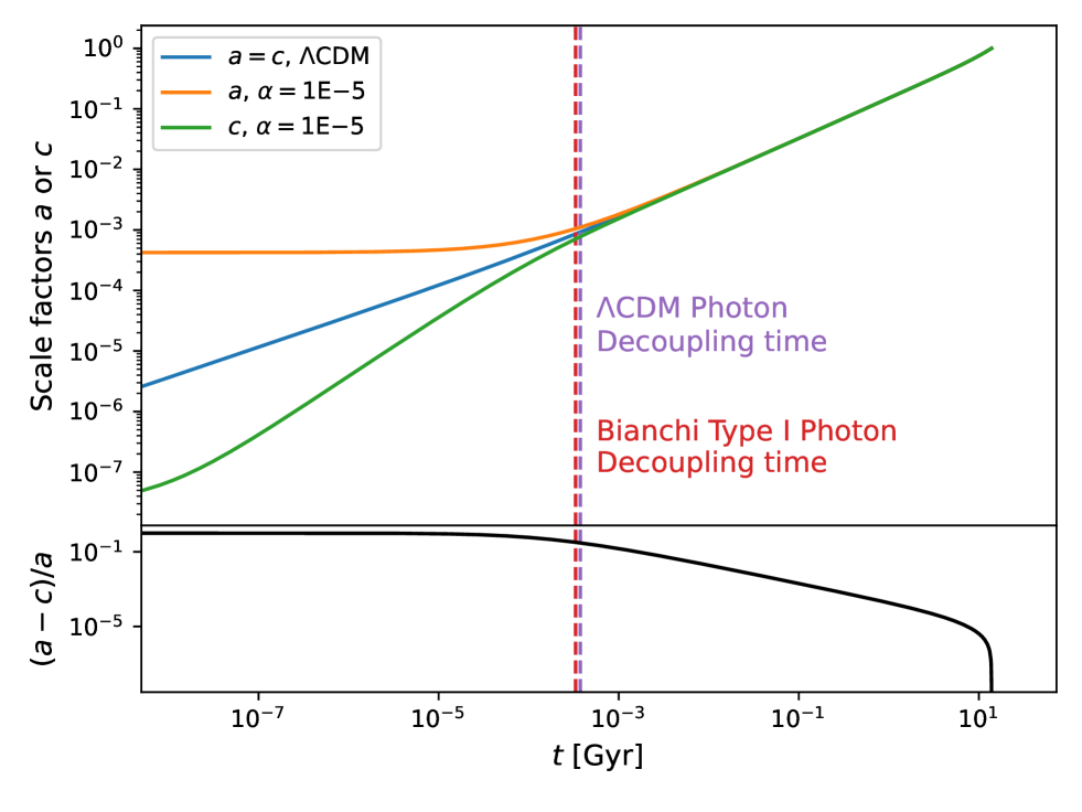
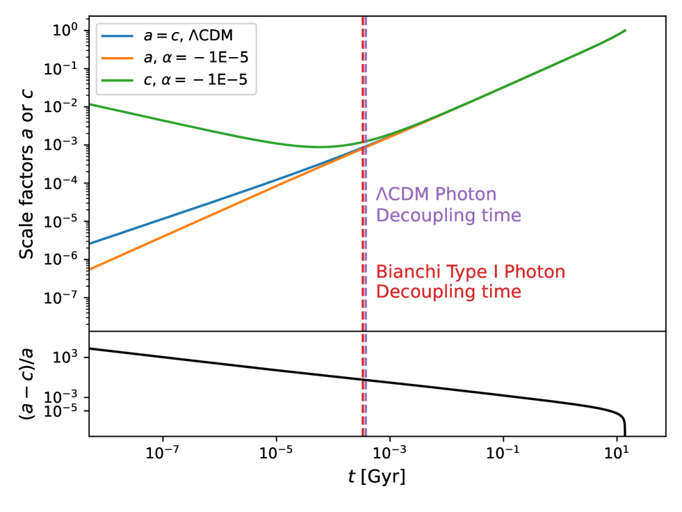
Figure 2: Expansion histories of $\Lambda$CDM and anisotropic universes with $\alpha=\pm 10^{-5}$, $+$ ($-$) for the upper (bottom) figure. The bottom panel of each figure shows the fractional difference of the scale factors in the anisotropic universes. The photon decoupling time in each model is shown in the vertical dashed line. Here, $H_{x0}$ (or $\mathfrak{H}_{0}$ for $\Lambda$CDM) and the energy densities of all universes are from Planck TTTEEE+low l+low E.

Table 2 summarizes the MCMC result as well as the log-Bayesian evidence and Akaike information criterion (AIC). Log-Bayesian evidence and AIC are the model selection criteria, in particular

$$\text{AIC}=2k-2\ln\mathcal{L}_{\text{max}},$$ (67)

where $k$ is the number of parameters and $\mathcal{L}_{\text{max}}$ is the maximum likelihood of the model.

From Table 2, one can see that the mean and variance of the standard cosmological parameters ($H_{x0}$, $\omega_{b0}$, $\omega_{c0}$, $\omega_{m0}$) are consistent with the $\Lambda$CDM values for anisotropic priors. Moreover, the absolute anisotropy $|\alpha|$ is tightly constrained, with a 95% limit of $<$4.74\text{\times}{10}^{-10}$$ for Priors A and B combined. The constraint is almost 50 times weaker when the maximum temperature anisotropy is relaxed to ${10}^{-3}$. A pictorial representation of the MCMC result is shown in Fig. 3 and 4 which plot the one and two-dimensional marginalized distributions (68% and 95% contours) of the parameters under different priors. Besides, Table 2 provides the constraints on $\tilde{\Omega}_{\sigma 0}$ and $\delta_{ac}$ defined in Ref. [28] and [32]

$$\tilde{\Omega}_{\sigma 0}=\frac{(H_{x0}-H_{z0})^{2}}{(2H_{x0}+H_{z0})^{2}},$$ (68)

$$\delta_{ac}=\frac{2|H_{x}(t_{*})-H_{z}(t_{*})|}{H_{x}(t_{*})+H_{z}(t_{*})},$$ (69)

for comparison. We find that under the tight temperature anisotropy limit of $2\text{\times}{10}^{-5}$, our result ($\tilde{\Omega}_{\sigma 0}<$2.5\text{\times}{10}^{-20}$$, $\delta_{xz}<$2.7\text{\times}{10}^{-5}$$) generally agrees with those in Ref. [28, 32] ($\tilde{\Omega}_{\sigma 0}\lesssim$4\text{\times}{10}^{-20}$$, $\delta_{xz}\lesssim${10}^{-5}$$, respectively).

		$\delta T/T<$2\text{\times}{10}^{-5}$$		$\delta T/T<${10}^{-3}$$
Parameter	$\Lambda$CDM	Prior A	Prior B	Prior C	Prior D
$H_{x0}$	$68.21\pm 0.96$	$68.15\pm 0.98$	$68.18\pm 0.98$	$68.17\pm 0.97$	$68.16\pm 0.98$
$\omega_{b0}$	$0.0220\pm 0.0013$	$0.0220\pm 0.0014$	$0.0220\pm 0.0014$	$0.0220\pm 0.0014$	$0.0220\pm 0.0013$
$\omega_{c0}$	$0.1156^{+0.0012}_{-0.0014}$	$0.1157^{+0.0012}_{-0.0013}$	$0.1156\pm 0.0013$	$0.1156\pm 0.0013$	$0.1156\pm 0.0012$
$|\alpha|$ (95% C.I.)	—	$<4.72\cdot 10^{-10}$	$<4.74\cdot 10^{-10}$	$<2.37\cdot 10^{-8}$	$<2.36\cdot 10^{-8}$
$\omega_{m0}$	$0.1377^{+0.0022}_{-0.0025}$	$0.1376^{+0.0022}_{-0.0026}$	$0.1376\pm 0.0024$	$0.1376\pm 0.0024$	$0.1376\pm 0.0023$
$\delta_{xz}$ (95% C.I.)	—	$<2.69\cdot 10^{-5}$	$<2.70\cdot 10^{-5}$	$<0.00136$	$<0.00134$
$\tilde{\Omega}_{\sigma 0}$ (95% C.I.)	—	$<2.48\cdot 10^{-20}$	$<2.50\cdot 10^{-20}$	$<6.26\cdot 10^{-17}$	$<6.21\cdot 10^{-17}$
$\ln\mathcal{E}$	$-555.32$	$-554.97$	$-555.01$	$-554.47$	$-554.50$
AIC	$1090.47$	$1092.45$	$1092.46$	$1092.45$	$1092.44$

Table 2: Means and 68% limits of the cosmological parameters corresponding to the $\Lambda$CDM model and the anisotropic priors under different maximum temperature anisotropy $\delta T/T$. For $\alpha$, $\tilde{\Omega}_{\sigma 0}$ and $\delta_{ac}$, the 95% upper limits are shown. The log-Bayesian evidence and AIC are also listed. Note that for Priors A and C, $\alpha$ is negative.

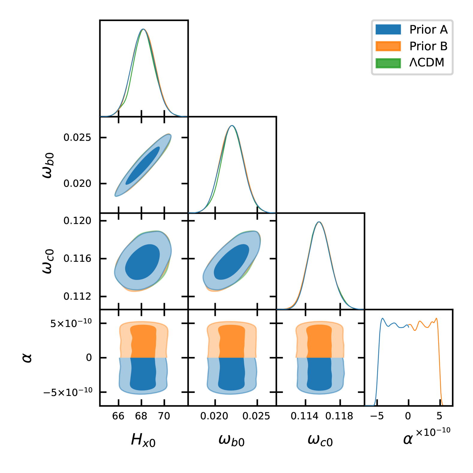
Figure 3: One and two-dimensional marginalized distributions (68% and 95% contours) of the cosmological parameters for the $\Lambda$CDM model and the anisotropic model with Priors A and B.

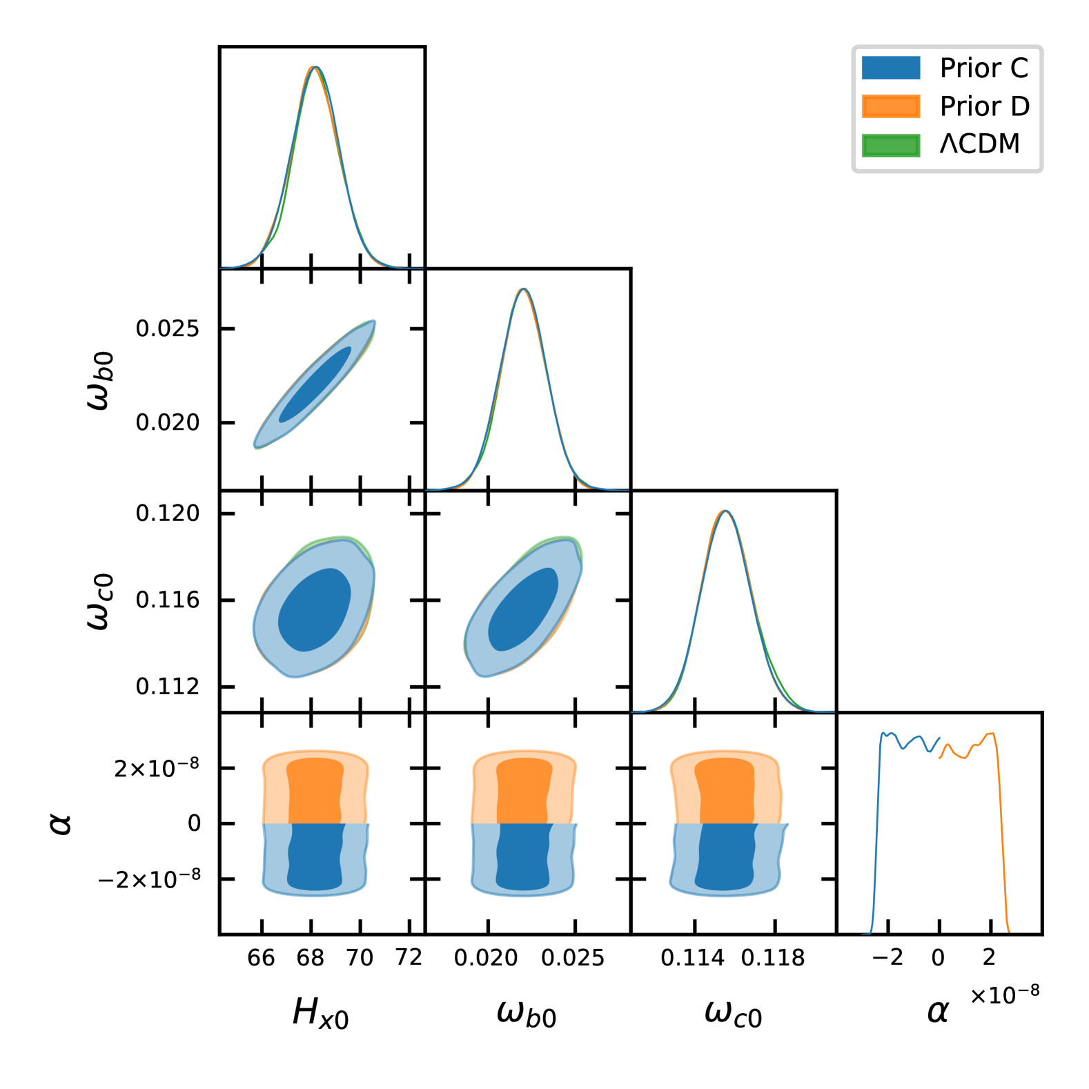
Figure 4: Same as Fig. 3, but for Priors C and D.

To determine whether the anisotropic model is preferred over $\Lambda$CDM, one would need to consider the Bayes factor or AIC. The Bayes factor $\mathcal{B}$ is defined as the ratio of the evidence of the model under consideration to that of the fiducial model [71]. A ratio larger than 1 implies the model under consideration is favored over the fiducial [71]. In contrary, a positive $\Delta\text{AIC}\equiv\text{AIC}_{\text{model}}-\text{AIC}_{\text{fiducial}}$ implies the model under consideration is disfavored [72]. We find that regardless of the prior choice, the axial symmetric Bianchi Type I model is consistently not worth a bare mention compared to $\Lambda$CDM, with a log-Bayes factor $<$1$$ and a $\Delta$AIC $<$2$$. The lack of preference over $\Lambda$CDM mainly stems from the fact that the $\Lambda$CDM can produce a full-sky averaged angular acoustic scale $\langle\theta_{*}\rangle$ as good as the axially symmetric Bianchi Type I, within Planck error bars. We expect that the anisotropic model might be preferred over $\Lambda$CDM to a large extent if the $\theta_{*}$ at each direction is studied instead of taking the full sky average. Observations are already able to detect anisotropy in $100\theta_{\text{MC}}$, which is approximately $100\theta_{*}$, by dividing the sky into $48$ half-skies [17]. It would be interesting to follow up on this direction in the future.

$\ln\mathcal{B}$	Evidence against fiducial
0 to 1	Not worth a bare mention
1 to 3	Positive evidence
3 to 5	Strong evidence
$>5$	Very strong evidence
$\Delta\text{AIC}$	Evidence for fiducial
0 to 2	Substantial evidence
4 to 7	Considerably less evidence
$>10$	Essentially no evidence

Table 3: Jeffery’s scale for Bayes factor [71] alongside the correspondence between $\Delta$AIC and evidence for the fiducial [72].

In the following, we discuss the significance of the modifications in the definitions of observables and the recombination history. First, it must be stressed that the proper way to define observables is through considering geodesics. One should not take the definitions in the FLRW metric and promote the FLRW scale factor $\mathfrak{a}$ to the geometric averaged scale factor $\tilde{a}$ without any justification. Although the definitions agree with each other by reducing to the standard ones in the FLRW metric when anisotropy could be negligible, it is important to distinguish them especially when the anisotropy is large, suggested by some observations such as those in Ref. [17]. For instance, we consider the means of parameters in Prior A and C and study how the CMB angular acoustic scales differ. In Prior A, the difference in $100\langle\theta_{*}\rangle$ between the definitions is only around $7\text{\times}{10}^{-3}$%, substantially smaller than the percentage error of Planck (0.03%)[36]. However, in Prior C which is 50 times more anisotropic than the former, the difference in $100\langle\theta_{*}\rangle$ grows to a considerable level of 0.2%, an order larger than the error of Planck.

In contrast, the modified recombination history has little to no impact on the last scattering time $t_{*}$. Our parameter means from MCMC suggest that the last scattering time $t_{*}$ differ by $<0.01\%$ in all prior sets, compared to our $\Lambda$CDM MCMC result, $t_{*}\sim$3.79\text{\times}{10}^{-4}\text{\,}\mathrm{Gyr}$$. Moreover, the corresponding redshifts as defined in Eq. 27 are consistent with that from our $\Lambda$CDM result, $\tilde{z}_{*}\sim 1085$. Thus, under realistic anisotropy, one can safely ignore the change in the recombination history of the Bianchi Type I model. Since the thermodynamics are not significantly changed, we redo the MCMC analysis for $\delta T/T<$2\text{\times}{10}^{-3}$$ and the $\Lambda$CDM case using the codes HyRec [38, 37] and modified CLASS [48], based on the equations prescribed in section II.1 and Ref. [28] for a more sophisticated atomic treatment. The results, presented in Appx. A, are generally consistent with Table 2, indicating our thermodynamics treatment which follows Peebles’ three-level atom model, is decent. We also point out that since there is no strong correlation between $\alpha$ and $\omega_{b0}$ for the range of anisotropy we considered, varying baryon density only introduces larger error bars to the standard cosmological parameters.

This work is motivated by the anisotropy observed in global and local measurements, particularly directional dependencies in the Hubble constant [17, 22, 23, 24, 25]. A meaningful comparison can be made between our constraints and the observed anisotropies. Generally, local observations on SNeIa [22, 23, 24, 25] find that the Hubble constant varies by $\sim$1\text{\,}\mathrm{km}\text{\,}{\mathrm{s}}^{-1}\text{\,}{\mathrm{Mpc}}^{-1}$$ with direction, equivalent to a fractional difference of $\sim 1\%$. Our result, on the other hand, suggests that the fractional difference is no more than $\sim${10}^{-6}$$% even when considering the looser limits, i.e., results from Priors C and D. Hence, the Bianchi Type I model is definitely inadequate in explaining the observed SNeIa anisotropy, which is not surprising. Recall that the Bianchi Type I model isotropizes at late times. To achieve a $1\text{\,}\mathrm{km}\text{\,}{\mathrm{s}}^{-1}\text{\,}{\mathrm{Mpc}}^{-1}$ variation in the Hubble constant, the universe must be highly anisotropic at late times and even more so at early times, disrupting physics at the last scattering surface. Therefore, the observed anisotropy in SNeIa needs a model that anisotropize at late times to explain, such as through the presence of anisotropic matter sources [34]. Alternatively, the anisotropy may just be due to local effects, but it is challenging to explain its alignment with CMB multipoles.

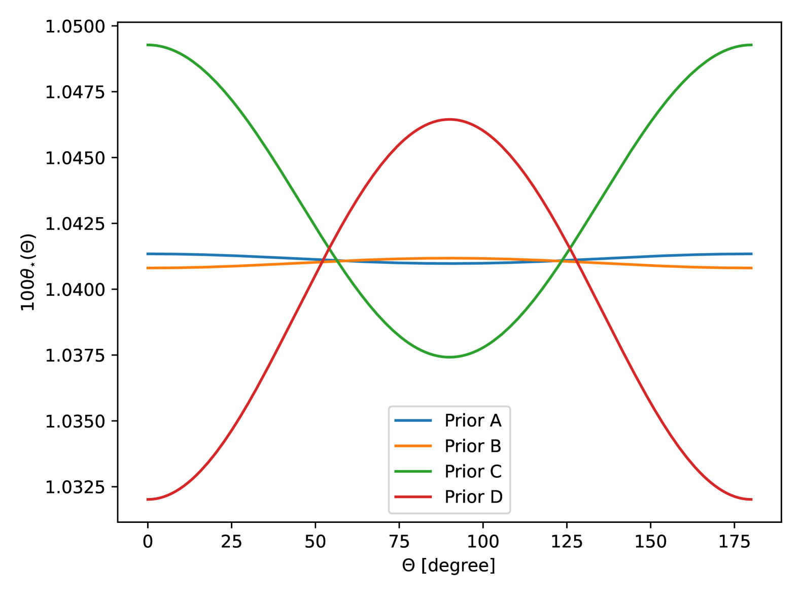
Figure 5: Directional variation of $100\theta_{*}$ from mean values of different priors.

Comparing our results with the observed CMB anisotropies in $\{\Omega_{b}h^{2},\Omega_{c}h^{2},n_{s},100\theta_{\mathrm{MC}},\tau,\allowbreak\ln{(10^{10}A_{s})},\allowbreak H_{0}\}$ is challenging, as these are derived from MCMC analyzes of Planck half-skies power spectra with the standard $\Lambda$CDM cosmology [17]. If the universe is indeed anisotropic, the MCMC result obtained using the $\Lambda$CDM model is inconsistent and, thus, not representative. Regardless, one can still compare our result with Ref. [17]. Clearly, our model assumes that energy densities have no directional variation which disagrees with Ref. [17]. Moreover, Ref. [17] observed a variation in $H_{0}$ with amplitude $\sim$5\text{\,}\mathrm{km}\text{\,}{\mathrm{s}}^{-1}\text{\,}{\mathrm{Mpc}}^{-1}$$. Again, such a large variation is unreachable in our model. However, it may be more important to compare the anisotropy in $100\theta_{\mathrm{MC}}$ due to its geometric nature and robustness to different cosmologies [36]. The large directional variations in Hubble constant and energy densities may be the consequence of fitting the standard $\Lambda$CDM cosmology to the observed $100\theta_{\mathrm{MC}}$ anisotropy instead. From Fig. 5, we can see that Prior A (B) predicts a variation roughly between $1.04101.0413$ ($1.04081.0412$) while it is between $1.03741.0493$($1.03201.0464$) for Prior C (D). To compare, Ref. [17] reports a fluctuation from $1.03911.0423$, slightly larger than that from Prior A and B. Hence, if we relax the temperature anisotropy constraint, say by including the effect of a small non-kinematic dipole, our model can explain the amplitude of the observed anisotropy in $100\theta_{\mathrm{MC}}$. Yet, our axial symmetric model cannot explain the azimuthal dependency observed [17]. It would be our next focus to study such anisotropy in $100\theta_{\mathrm{MC}}$ with the fully asymmetry Bianchi Type I model.

To further improve the constraints on the anisotropic model with currently available data, one needs to develop the theory and cosmological codes for BBN and the CMB power spectra under the Bianchi Type I model. Current BBN and cosmological codes such as PArthENoPE and CLASS [73, 48] assume the FLRW metric. Significant work is needed to modify the codes for the Bianchi Type I metric, especially for CLASS which adopts FLRW scale factor $\mathfrak{a}$ as the temporal coordinate. For an order-of-magnitude constraint on $\tilde{\Omega}_{\sigma 0}$ and $\delta_{xy}$, one can refer to Ref. [28, 32] since our result is consistent with theirs under a maximum temperature anisotropy $\delta T/T$ of $2\text{\times}{10}^{-5}$. However, their analysis should be taken with caution since the authors assume that the BBN time or redshift is not affected by the anisotropy [28, 32]. Without proper study, the possibility of a drastically modified BBN history with similar element fractions cannot be ruled out, especially since BBN does not have a strong implication on isotropy like CMB. Meanwhile, the constraints can be improved if one detects primordial relics such as primordial neutrinos. Their energy would have directional dependency due to the anisotropic dilution after freeze out [32]. Contrarily, if the CMB dipole is found to have a non-zero kinematic contribution, it would be a strong piece of evidence for the anisotropic universe and possibly for the Bianchi Type I model. Rigorous studies on BBN, which occurred at a more anisotropic time than CMB’s, would be particularly valuable. The ongoing Euclid mission and the future Roman mission could provide crucial tests on the kinematic nature of CMB by measuring the Cosmic Infrared Background (CIB) dipole [74, 75, 76].

VI Conclusion

In this paper, we present a self-consistent constraint on the axially symmetric Bianchi Type I model. Instead of assuming a fixed recombination redshift or time, we calculate the recombination history with a modified Peebles’ formalism based on the anisotropic model. Moreover, we improve on previous works [28, 30, 33, 31] by constructing distances and observables, including CMB and BAO angular acoustic scales, based on geodesic, achieving truly directional dependent observables. To constrain the model, we construct and modify existing likelihood codes to compare the full-sky averaged observables with observations in companion with MCMC. Our key conclusions are summarized below:

1. By considering full-sky averages, the axially symmetric Bianchi Type I model is not worth a bare mention compared to the $\Lambda$CDM model for maximum allowed temperature anisotropy $\delta T/T<$2\text{\times}{10}^{-5}$$ and ${10}^{-3}$.

2. The anisotropy parameter $\alpha$ is tightly constrained with an upper bound in $|\alpha|$ of $4.7\text{\times}{10}^{-10}$ ($2.4\text{\times}{10}^{-8}$) at $95\%$ confidence level when the maximum temperature anisotropy $\delta T/T$ equals $2\text{\times}{10}^{-5}$ (${10}^{-3}$). The tighter constraint is generally consistent with Ref. [28, 17] obtained using similar temperature anisotropy.

3. We stress the importance of geodesic-based observables in anisotropic cosmology by showing that the geodesic-based CMB angular scale is drastically different from that defined by drawing simple parallels with $\Lambda$CDM [28, 30, 33, 31] under a non-negligible anisotropy.

4. The modifications in the recombination history are insignificant, even under a large anisotropy such that maximum temperature anisotropy $\delta T/T$ is comparable to the CMB dipole.

5. The anisotropic model cannot account for the observed directional dependency in SNeIa observations [22, 23, 24, 25]. On the other hand, the magnitude of the $100\theta_{\mathrm{MC}}$ anisotropy observed in CMB [17] can be explained with our model with a maximum temperature anisotropy $\delta T/T$ slightly larger than $2\text{\times}{10}^{-5}$.

Appendix A MCMC Results with CLASS Thermodynamics

Since Peebles’ formalism neglects most atomic transitions and considers only a three-level Hydrogen atom [39, 40, 41], it is crucial to verify that our results are consistent with those obtained from a more accurate thermodynamics code that incorporates contributions from Helium and a multi-level atomic treatment. As demonstrated in Sec. V, the thermodynamics remain virtually unchanged compared to the $\Lambda$CDM framework. Consequently, we employ the recombination code HyRec [38, 37] alongside a modified version of the cosmological code CLASS [48] according to section II.1 and Ref. [28]. We then perform MCMC analyses on both the $\Lambda$CDM model and the anisotropic model, with the condition $\delta T/T<$2\text{\times}{10}^{-5}$$. The results, which are consistent with those derived using Peebles’ formalism, are presented in Table 4. This confirms that our findings are robust against more sophisticated treatments of thermodynamics and recombination.

	Peebles’ formalism			HyRec + modified CLASS
Parameter	$\Lambda$CDM	Prior A	Prior B	$\Lambda$CDM HR	Prior A HR	Prior B HR
$H_{x0}$	$68.21\pm 0.96$	$68.15\pm 0.98$	$68.18\pm 0.98$	$68.24\pm 0.94$	$68.20\pm 0.97$	$68.16\pm 0.99$
$\omega_{b0}$	$0.0220\pm 0.0013$	$0.0220\pm 0.0014$	$0.0220\pm 0.0014$	$0.0221\pm 0.0014$	$0.0220\pm 0.0014$	$0.0220\pm 0.0014$
$\omega_{c0}$	$0.1156^{+0.0012}_{-0.0014}$	$0.1157^{+0.0012}_{-0.0013}$	$0.1156\pm 0.0013$	$0.1157\pm 0.0012$	$0.1157\pm 0.0011$	$0.1157\pm 0.0012$
$|\alpha|$ (95% C.I.)	—	$<4.72\cdot 10^{-10}$	$<4.74\cdot 10^{-10}$	—	$<4.72\cdot 10^{-10}$	$<4.72\cdot 10^{-10}$
$\omega_{m0}$	$0.1377^{+0.0022}_{-0.0025}$	$0.1376^{+0.0022}_{-0.0026}$	$0.1376\pm 0.0024$	$0.1378^{+0.0020}_{-0.0023}$	$0.1377\pm 0.0022$	$0.1377\pm 0.0022$
$\delta_{xz}$ (95% C.I.)	—	$<2.69\cdot 10^{-5}$	$<2.70\cdot 10^{-5}$	—	$<2.69\cdot 10^{-5}$	$<2.69\cdot 10^{-5}$
$\tilde{\Omega}_{\sigma 0}$ (95% C.I.)	—	$<2.48\cdot 10^{-20}$	$<2.50\cdot 10^{-20}$	—	$<2.48\cdot 10^{-20}$	$<2.48\cdot 10^{-20}$
$\ln\mathcal{E}$	$-555.32$	$-554.97$	$-555.01$	$-555.26$	$-554.94$	$-554.95$
AIC	$1090.47$	$1092.46$	$1092.46$	$1090.48$	$1092.46$	$1092.50$

Table 4: Similar to Table 2, but comparing MCMC results from Peebles’ recombination formalism and HyRec with the modified CLASS. ‘HR’ here refers to the cases with HyRec and modified CLASS.

References

- Bielewicz et al. [2005] P. Bielewicz, H. K. Eriksen, A. J. Banday, K. M. Górski, and P. B. Lilje, Multipole vector anomalies in the first-year WMAP data: A cut-sky analysis, Astrophysical. J. 635, 750 (2005).
- de Oliveira-Costa et al. [2004] A. de Oliveira-Costa, M. Tegmark, M. Zaldarriaga, and A. Hamilton, Significance of the largest scale CMB fluctuations in WMAP, Phys. Rev. D 69, 063516 (2004).
- Tegmark et al. [2003] M. Tegmark, A. de Oliveira-Costa, and A. J. S. Hamilton, High resolution foreground cleaned CMB map from WMAP, Phys. Rev. D 68, 123523 (2003).
- Wiaux et al. [2006] Y. Wiaux, P. Vielva, E. Martínez-González, and P. Vandergheynst, Global universe anisotropy probed by the alignment of structures in the cosmic microwave background, Phys. Rev. Lett. 96, 151303 (2006).
- Hansen et al. [2004] F. K. Hansen, A. J. Banday, and K. M. Górski, Testing the cosmological principle of isotropy: local power-spectrum estimates of the WMAP data, Mon. Not. R. Astron. Soc. 354, 641 (2004).
- Eriksen et al. [2004] H. K. Eriksen, F. K. Hansen, A. J. Banday, K. M. Górski, and P. B. Lilje, Asymmetries in the cosmic microwave background anisotropy field, Astrophysical. J. 605, 14 (2004).
- Bernui, A. et al. [2006] Bernui, A., Villela, T., Wuensche, C. A., Leonardi, R., and Ferreira, I., On the cosmic microwave background large-scale angular correlations, Astron. Astrophys. 454, 409 (2006).
- Bernui [2008] A. Bernui, Anomalous CMB north-south asymmetry, Phys. Rev. D 78, 063531 (2008).
- Bunn and Scott [2000] E. F. Bunn and D. Scott, A preferred-direction statistic for sky maps, Mon. Not. R. Astron. Soc. 313, 331 (2000).
- Bernui et al. [2007] A. Bernui, B. Mota, M. J. Reboucas, and R. Tavakol, Mapping the large-scale anisotropy in the WMAP data, Astron. Astrophys. 464, 479 (2007).
- Hansen et al. [2009] F. Hansen, A. Banday, K. Gorski, H. Eriksen, and P. Lilje, Power asymmetry in cosmic microwave background fluctuations from full sky to sub-degree scales: is the universe isotropic?, Astrophysical. J. 704, 1448 (2009).
- Axelsson et al. [2013] M. Axelsson, Y. Fantaye, F. Hansen, A. Banday, H. Eriksen, and K. Gorski, Directional dependence of CDM cosmological parameters, Astrophysical. J. Lett. 773, L3 (2013).
- Naselsky et al. [2012] P. Naselsky, W. Zhao, J. Kim, and S. Chen, Is the cosmic microwave background asymmetry due to the kinematic dipole?, Astrophysical. J. 749, 31 (2012).
- Zhao [2014] W. Zhao, Directional dependence of CMB parity asymmetry, Phys. Rev. D 89, 023010 (2014).
- Cheng et al. [2016] C. Cheng, W. Zhao, Q.-G. Huang, and L. Santos, Preferred axis of CMB parity asymmetry in the masked maps, Phys. Lett. B 757, 445 (2016).
- Aluri et al. [2017] P. K. Aluri, J. P. Ralston, and A. Weltman, Alignments of parity even/odd-only multipoles in CMB, Mon. Not. R. Astron. Soc. 472, 2410 (2017).
- Yeung and Chu [2022] S. Yeung and M.-C. Chu, Directional variations of cosmological parameters from the planck CMB data, Phys. Rev. D 105, 083508 (2022).
- Kashlinsky et al. [2008] A. Kashlinsky, F. Atrio-Barandela, D. Kocevski, and H. Ebeling, A measurement of large-scale peculiar velocities of clusters of galaxies: results and cosmological implications, Astrophysical. J. 686, L49 (2008).
- Watkins et al. [2009] R. Watkins, H. A. Feldman, and M. J. Hudson, Consistently large cosmic flows on scales of 100 h- 1 mpc: a challenge for the standard CDM cosmology, Mon. Not. R. Astron. Soc. 392, 743 (2009).
- Hutsemékers et al. [2005] D. Hutsemékers, R. Cabanac, H. Lamy, and D. Sluse, Mapping extreme-scale alignments of quasar polarization vectors, Astron. Astrophys. 441, 915 (2005).
- Antoniou and Perivolaropoulos [2010] I. Antoniou and L. Perivolaropoulos, Searching for a cosmological preferred axis: Union2 data analysis and comparison with other probes, J. Cosmol. Astropart. Phys. 2010 (12), 012.
- Javanmardi et al. [2015] B. Javanmardi, C. Porciani, P. Kroupa, and J. Pflamm-Altenburg, Probing the isotropy of cosmic acceleration traced by Type Ia supernovae, Astrophysical. J. 810, 47 (2015).
- Krishnan et al. [2022] C. Krishnan, R. Mohayaee, E. Ó. Colgáin, M. Sheikh-Jabbari, and L. Yin, Hints of FLRW breakdown from supernovae, Phys. Rev. D 105, 063514 (2022).
- Luongo et al. [2022] O. Luongo, M. Muccino, E. O. Colgáin, M. M. Sheikh-Jabbari, and L. Yin, Larger values in the CMB dipole direction, Phys. Rev. D 105, 103510 (2022).
- Hu et al. [2024] J. Hu, Y. Wang, J. Hu, and F. Wang, Testing the cosmological principle with the pantheon+ sample and the region-fitting method, Astron. Astrophys. 681, A88 (2024).
- Zhao and Santos [2016] W. Zhao and L. Santos, Preferred axis in cosmology, arXiv preprint arXiv:1604.05484 (2016), arXiv:1604.05484 [astro-ph.CO] .
- Perivolaropoulos and Skara [2022] L. Perivolaropoulos and F. Skara, Challenges for CDM: An update, New Astronomy Reviews 95, 101659 (2022).
- Akarsu et al. [2019] Ö. Akarsu, S. Kumar, S. Sharma, and L. Tedesco, Constraints on a Bianchi type I spacetime extension of the standard CDM model, Phys. Rev. D 100, 023532 (2019).
- Shekh and Chirde [2020] S. H. Shekh and V. R. Chirde, Accelerating bianchi type dark energy cosmological model with cosmic string in gravity, Astrophysics and Space Science 365, 10.1007/s10509-020-03772-y (2020).
- Sarmah and Goswami [2022] P. Sarmah and U. D. Goswami, Bianchi type i model of universe with customized scale factors, Modern Physics Letters A 37, 10.1142/s0217732322501346 (2022).
- Koussour et al. [2023] M. Koussour, S. Shekh, M. Govender, and M. Bennai, Thermodynamical aspects of bianchi type-i universe in quadratic form of f(q) gravity and observational constraints, Journal of High Energy Astrophysics 37, 15–24 (2023).
- Hertzberg and Loeb [2024] M. P. Hertzberg and A. Loeb, Constraints on an anisotropic universe, Phys. Rev. D 109, 083538 (2024).
- Yadav [2023] V. Yadav, Measuring hubble constant in an anisotropic extension of CDM model, Physics of the Dark Universe 42, 101365 (2023).
- Koivisto and Mota [2008] T. Koivisto and D. F. Mota, Anisotropic dark energy: dynamics of the background and perturbations, J. Cosmol. Astropart. Phys. 2008 (06), 018.
- Russell et al. [2014] E. Russell, C. B. Kılınç, and O. K. Pashaev, Bianchi I model: an alternative way to model the present-day Universe, Mon. Not. R. Astron. Soc. 442, 2331 (2014).
- Aghanim, N. et al. [2020] Aghanim, N. et al. (Planck), Planck 2018 results - vi. cosmological parameters, Astron. Astrophys. 641, A6 (2020).
- Lee and Ali-Haïmoud [2020] N. Lee and Y. Ali-Haïmoud, hyrec-2: A highly accurate sub-millisecond recombination code, Phys. Rev. D 102, 083517 (2020).
- Ali-Haïmoud and Hirata [2011] Y. Ali-Haïmoud and C. M. Hirata, Hyrec: A fast and highly accurate primordial hydrogen and helium recombination code, Phys. Rev. D 83, 043513 (2011).
- Peebles [1968] P. J. E. Peebles, Recombination of the Primeval Plasma, Astrophys. J. 153, 1 (1968).
- Baumann [2022] D. Baumann, Cosmology (Cambridge University Press, 2022).
- Weinberg [2008] S. Weinberg, Cosmology (OUP Oxford, 2008).
- Ade, P. A. R. et al. [2014] Ade, P. A. R. et al. (Planck), Planck 2013 results. xvi. cosmological parameters, Astron. Astrophys. 571, A16 (2014).
- Ade, P. A. R. et al. [2016] Ade, P. A. R. et al. (Planck), Planck 2015 results - xiii. cosmological parameters, Astron. Astrophys. 594, A13 (2016).
- Delliou et al. [2020] M. L. Delliou, M. Deliyergiyev, and A. del Popolo, An anisotropic model for the universe, Symmetry 12, 10.3390/sym12101741 (2020).
- Adame et al. [2024a] A. G. Adame et al. (DESI), DESI 2024 VI: Cosmological Constraints from the Measurements of Baryon Acoustic Oscillations, arXiv preprint arXiv:2404.03002 (2024a), arXiv:2404.03002 [astro-ph.CO] .
- Hindmarsh [1983] A. C. Hindmarsh, Odepack, a systemized collection of ode solvers, Scientific computing (1983).
- Petzold [1983] L. Petzold, Automatic selection of methods for solving stiff and nonstiff systems of ordinary differential equations, SIAM journal on scientific and statistical computing 4, 136 (1983).
- Blas et al. [2011] D. Blas, J. Lesgourgues, and T. Tram, The cosmic linear anisotropy solving system (CLASS). part ii: approximation schemes, J. Cosmol. Astropart. Phys. 2011 (07), 034.
- Torrado and Lewis [2019] J. Torrado and A. Lewis, Cobaya: Bayesian analysis in cosmology, Astrophysics Source Code Library, record ascl:1910.019 (2019).
- Torrado and Lewis [2021] J. Torrado and A. Lewis, Cobaya: Code for bayesian analysis of hierarchical physical models, J. Cosmol. Astropart. Phys. 2021 (05), 057.
- Lewis and Bridle [2002] A. Lewis and S. Bridle, Cosmological parameters from CMB and other data: A Monte Carlo approach, Phys. Rev. D 66, 103511 (2002).
- Lewis [2013] A. Lewis, Efficient sampling of fast and slow cosmological parameters, Phys. Rev. D 87, 103529 (2013).
- Lewis [2019] A. Lewis, Getdist: A Python package for analysing Monte Carlo samples, arXiv preprint arXiv:1910.13970 (2019), arXiv:1910.13970 [astro-ph.IM] .
- Heavens et al. [2017] A. Heavens, Y. Fantaye, A. Mootoovaloo, H. Eggers, Z. Hosenie, S. Kroon, and E. Sellentin, Marginal likelihoods from Monte Carlo Markov Chains, arXiv preprint arXiv:1704.03472 (2017), arXiv:1704.03472 [stat.CO] .
- Wald [1983] R. M. Wald, Asymptotic behavior of homogeneous cosmological models in the presence of a positive cosmological constant, Phys. Rev. D 28, 2118 (1983).
- Adame et al. [2024b] A. G. Adame et al. (DESI), DESI 2024 IV: Baryon Acoustic Oscillations from the Lyman Alpha Forest, arXiv preprint arXiv:2404.03001 (2024b), arXiv:2404.03001 [astro-ph.CO] .
- Adame et al. [2024c] A. G. Adame et al. (DESI), DESI 2024 III: Baryon Acoustic Oscillations from Galaxies and Quasars, arXiv preprint arXiv:2404.03000 (2024c), arXiv:2404.03000 [astro-ph.CO] .
- Alam and others [eBOSS Collaboration] S. Alam and others (eBOSS Collaboration) (eBOSS), Completed SDSS-IV extended Baryon Oscillation Spectroscopic Survey: Cosmological implications from two decades of spectroscopic surveys at the Apache Point Observatory, Phys. Rev. D 103, 083533 (2021).
- Ross et al. [2015] A. J. Ross, L. Samushia, C. Howlett, W. J. Percival, A. Burden, and M. Manera, The clustering of the SDSS DR7 main Galaxy sample – I. A 4 per cent distance measure at , Mon. Not. R. Astron. Soc. 449, 835 (2015).
- Beutler et al. [2012] F. Beutler, C. Blake, M. Colless, D. H. Jones, L. Staveley-Smith, G. B. Poole, L. Campbell, Q. Parker, W. Saunders, and F. Watson, The 6df galaxy survey: measurements of the growth rate and 8, Mon. Not. R. Astron. Soc. 423, 3430 (2012).
- M. Moresco et al. [2012] M. Moresco et al., Improved constraints on the expansion rate of the universe up to z 1.1 from the spectroscopic evolution of cosmic chronometers, J. Cosmol. Astropart. Phys. 2012 (08), 006.
- Zhang et al. [2014] C. Zhang, H. Zhang, S. Yuan, S. Liu, T.-J. Zhang, and Y.-C. Sun, Four new observationalh(z) data from luminous red galaxies in the sloan digital sky survey data release seven, Res. Astron. Astrophys. 14, 1221 (2014).
- Simon et al. [2005] J. Simon, L. Verde, and R. Jimenez, Constraints on the redshift dependence of the dark energy potential, Phys. Rev. D. 71, 10.1103/PhysRevD.71.123001 (2005).
- Moresco et al. [2016] M. Moresco, L. Pozzetti, A. Cimatti, R. Jimenez, C. Maraston, L. Verde, D. Thomas, A. Citro, R. Tojeiro, and D. Wilkinson, A 6% measurement of the hubble parameter at z 0.45: direct evidence of the epoch of cosmic re-acceleration, J. Cosmol. Astropart. Phys. 2016 (05), 014.
- Ratsimbazafy et al. [2017] A. L. Ratsimbazafy, S. I. Loubser, S. M. Crawford, C. M. Cress, B. A. Bassett, R. C. Nichol, and P. Väisänen, Age-dating luminous red galaxies observed with the southern african large telescope, Mon. Not. R. Astron. Soc. 467, 3239 (2017).
- Moresco [2015] M. Moresco, Raising the bar: new constraints on the hubble parameter with cosmic chronometers at z 2, Mon. Not. R. Astron. Soc. Lett. 450, L16 (2015).
- Delubac et al. [2015] T. Delubac et al., Baryon acoustic oscillations in the Lyforest of BOSS DR11 quasars, Astron. Astrophys. 574, A59 (2015).
- Font-Ribera et al. [2014] A. Font-Ribera et al., Quasar-Lyman forest cross-correlation from BOSS DR11: Baryon acoustic oscillations, J. Cosmol. Astropart. Phys. 2014 (05), 027.
- Alam et al. [2017] S. Alam et al., The clustering of galaxies in the completed SDSS-III baryon oscillation spectroscopic survey: cosmological analysis of the DR12 galaxy sample, Mon. Not. R. Astron. Soc. 470, 2617 (2017).
- Scolnic et al. [2018] D. M. Scolnic et al., The Complete Light-curve Sample of Spectroscopically Confirmed SNe Ia from Pan-STARRS1 and Cosmological Constraints from the Combined Pantheon Sample, Astrophys. J. 859, 101 (2018).
- Kass and Raftery [1995] R. E. Kass and A. E. Raftery, Bayes factors, Journal of the American Statistical Association 90, 773 (1995).
- Burnham et al. [1998] K. P. Burnham, D. R. Anderson, K. P. Burnham, and D. R. Anderson, Practical use of the information-theoretic approach (Springer, 1998).
- Consiglio et al. [2018] R. Consiglio, P. de Salas, G. Mangano, G. Miele, S. Pastor, and O. Pisanti, Parthenope reloaded, Computer Physics Communications 233, 237 (2018).
- Kashlinsky and Atrio-Barandela [2022] A. Kashlinsky and F. Atrio-Barandela, Probing the rest-frame of the universe with the near-ir cosmic infrared background, Mon. Not. R. Astron. Soc. Lett. 515, L11 (2022).
- Kashlinsky and others [Euclid Collaboration] A. Kashlinsky and others (Euclid Collaboration) (Euclid), Euclid preparation-xlvi. the near-infrared background dipole experiment with euclid, Astron. Astrophys. 689, A294 (2024).
- Akeson et al. [2019] R. Akeson et al., The wide field infrared survey telescope: 100 hubbles for the 2020s, arXiv preprint arXiv:1902.05569 (2019), arXiv:1902.05569 [astro-ph.IM] .
- Harris et al. [2020] C. R. Harris et al., Array programming with NumPy, Nature 585, 357 (2020).
- Virtanen et al. [2020] P. Virtanen et al., SciPy 1.0: Fundamental Algorithms for Scientific Computing in Python, Nature Methods 17, 261 (2020).
- Lam et al. [2015] S. K. Lam, A. Pitrou, and S. Seibert, Numba: A llvm-based python jit compiler, in Proceedings of the Second Workshop on the LLVM Compiler Infrastructure in HPC (2015) pp. 1–6.
- Hunter [2007] J. D. Hunter, Matplotlib: A 2d graphics environment, Computing in Science & Engineering 9, 90 (2007).