Continual Multimodal Contrastive Learning

Abstract

Multimodal contrastive learning (MCL) advances in aligning different modalities and generating multimodal representations in a joint space. By leveraging contrastive learning across diverse modalities, large-scale multimodal data enhances representational quality. However, a critical yet often overlooked challenge remains: multimodal data is rarely collected in a single process, and training from scratch is computationally expensive. Instead, emergent multimodal data can be used to optimize existing models gradually, i.e., models are trained on a sequence of modality pair data. We define this problem as Continual Multimodal Contrastive Learning (CMCL), an underexplored yet crucial research direction at the intersection of multimodal and continual learning. In this paper, we formulate CMCL through two specialized principles of stability and plasticity. We theoretically derive a novel optimization-based method, which projects updated gradients from dual sides onto subspaces where any gradient is prevented from interfering with the previously learned knowledge. Two upper bounds provide theoretical insights on both stability and plasticity in our solution. Beyond our theoretical contributions, we conduct experiments on multiple datasets by comparing our method against advanced continual learning baselines. The empirical results further support our claims and demonstrate the efficacy of our method. The code will be publicly available.

1 Introduction

Humans perceive the world in a multimodal way: capture and process information from what we see, hear, smell, and touch; machines are evolving towards multisensory processing to mimic this capability by leveraging specialized latent representations to interpret the world effectively [1, 2, 3, 4, 5, 6]. Multimodal contrastive learning (MCL) builds upon uni-modal [7, 8, 9] and cross-modal contrastive learning [10, 11], which demonstrates exceptional representational power and broad applicability. The core principle behind it is to bring modality pairs (e.g., vision-text or vision-audio data) from the same instance closer together while simultaneously pushing apart representations of different instances. Consequently, MCL constructs a unified representation space yet capable of accommodating diverse modalities [12, 13, 14, 15]. Such effective paradigms inspire researchers to explore how to collect more extensive multimodal data.

Extensive data support is critical for ensuring representational quality. Recent studies have focused on either compensating to the existing modality data [14, 15] or introducing the emergent ones [16]. Besides learning from scratch, collected data can also be incrementally introduced to gradually enhance a model’s capabilities, thereby resolving two significant challenges: 1) the difficulty of collecting all prepared multimodal data in a single process, and 2) the high computational expense associated with training on mixed datasets from initialization. With the emergent multimodal data, multimodal models can be progressively elevated via continual/incremental learning. Unfortunately, recent research in MCL primarily advances in an “all in one go” manner. Moreover, it is intractable for current continual learning methods to address this problem [17, 18, 19, 20], due to the inter-modal complexity and the task-agnostic constraints, where the objective of contrasting different modalities remains consistent over time.

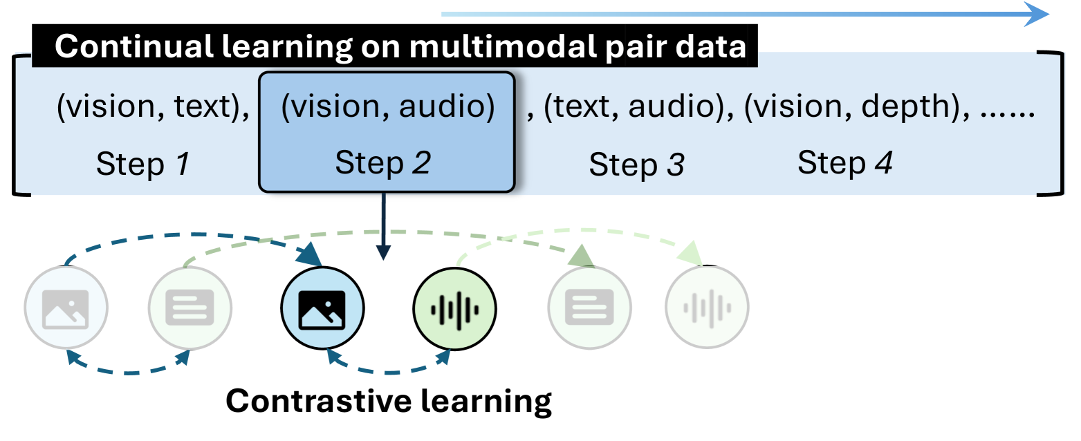
(a)

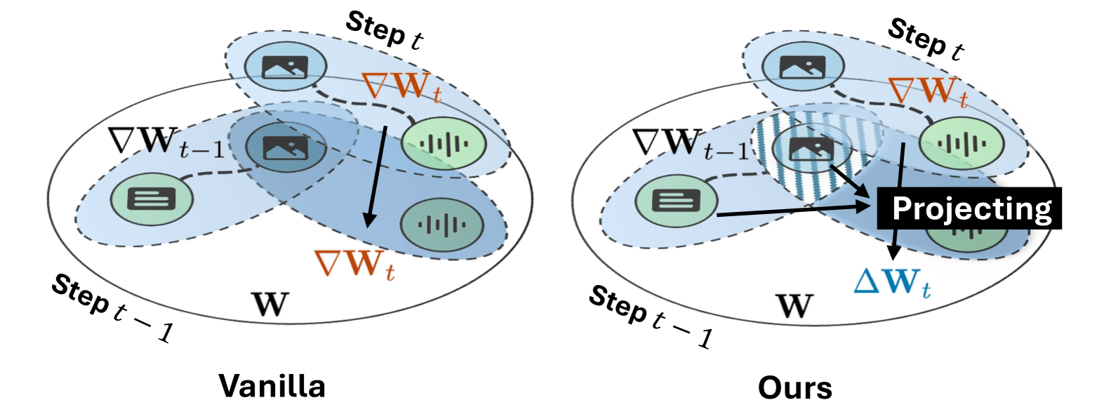
(b)

Figure 1: (a) The problem of Continual Multimodal Contrastive Learning (CMCL). Multimodal models learn from data step by step. At each step, the two modalities are aligned through contrastive learning. Different pairs of modalities are involved at different steps. (b) Our gradient-projection method (right) compared with the vanilla (left). Within the parameter space spanned by $\mathbf{W}$, the gradient updated at the previous step $\nabla\mathbf{W}_{t-1}$ is directly overridden in vanilla training. However, our method projects the new gradient $\nabla\mathbf{W}_{t}$ onto the non-effective subspaces of the old, denoting $\Delta\mathbf{W}_{t}$, to maintain both stability and plasticity in CMCL.

Aware of this, we pioneer the formulation of Continual Multimodal Contrastive Learning (CMCL) in this paper. In CMCL, a sequence of multimodal data is utilized for training. At each training step, two modalities are aligned through contrastive learning, and the new modality pair is subsequently integrated into the following step, as illustrated in Figure 1(a). We specify two definitions of stability and plasticity in CMCL. Here stability refers to the model’s capability to retain acquired knowledge over previously interacted modalities, while plasticity denotes that the model can learn effectively from new modality pairs. Building upon this foundation, we theoretically derive a novel CMCL method by projecting updated parameter gradients from dual sides onto specialized subspaces, as shown in Figure 1(b). We project gradients based on both their own modality knowledge and their interacted ones, i.e., a dual-sided projection. These inter-modality histories are utilized to construct the corresponding gradient projectors. Incorporating new data at the current training step within these projected subspaces does not adversely impact model performance on datasets from previous steps. Furthermore, we provide theoretical guarantees by establishing two bounds addressing stability and plasticity. These bounds substantiate our method’s effectiveness theoretically, further supported by empirical analyses. Besides, we showcase the flexibility of our method by extending it to any steps and any modality pairs thus achieving both efficacy and efficiency in practice. We conduct experiments on 7 datasets to evaluate our solution for classification and retrieval tasks. The results well justify our claims. The proposed method consistently achieves superior performance in plasticity and stability. Compared with previous state-of-the-art (SOTA) baselines of the continual learning field, it demonstrates remarkable results across multiple metrics.

Before delving into details, we clearly emphasize our contributions as follows:

• Conceptually, we take the initiative to formulate continual multimodal contrastive learning explicitly and provide specialized definitions of stability and plasticity that guide methodological development. Our work establishes a foundational framework for exploring this previously unaddressed problem and encourages future contributions to CMCL.

• Technically, we introduce a novel method that operates on the parameter gradients. These gradients are projected onto the subspaces where any updated gradients have no effect on the previous knowledge. This method is built upon existing modality-binding models and can be readily extendable to any training steps and modality pairs in the practical training procedure.

• Theoretically, we rigorously derive our method based on the fundamental requirements (stability and plasticity), supported by detailed theoretical proofs. Additionally, we provide two theoretical bounds that guarantee the objectives, which can be tightened in practice to reinforce our claim.

• Empirically, we conduct experiments on 7 datasets to evaluate the performance in the CMCL setting. Utilizing three modality-binding methods as backbones, we demonstrate superior performance compared to SOTA continual learning baselines, which confirms the effectiveness of our solution.

2 Preliminaries

Multimodal learning. Typical multimodal learning can be formulated as:

$$\mathbb{P}(\mathbf{x},y)\triangleq\mathbb{P}_{y|\mathbf{x}}\left(y\mid h\circ g(\mathbf{x})\right)\mathbb{P}_{\mathbf{x}}(\mathbf{x}),$$ (1)

where $g$ is the multimodal encoder that generates corresponding representation $\mathbf{z}$ given the input $\mathbf{x}$, and $h$ is the task mapping (e.g., linear classifier [11, 12] or even Large Language Models (LLMs) [21, 22, 23]). In general, $g$ is modal-agnostic. Here we use $g_{m}$ as the modal-specific encoder indicating that we do not make any assumption to a shared model architecture or parameters. For different modalities, a unified representation space is desired to facilitate the development of $h$, so that, one well-trained $h$ serves all $\{g_{m}\}_{m\in\mathcal{M}}$.

Modality-binding (modality pairs for training). Note that $g$ is normally implemented by modality-binding methods to obtain representations for different modalities in a unified space. These methods utilize paired data $\mathcal{X}^{m;m^{\prime}}=\{(\mathbf{x}^{m}_{1},\mathbf{x}^{m^{\prime}}_{1}),\dots\}\subset\mathcal{X}^{m}\times\mathcal{X}^{m^{\prime}}$ to optimize the contrastive objective derived from CLIP:

$$\mathcal{L}=-\log\frac{\exp(\mathbf{z}^{m\top}_{i}\mathbf{z}^{m^{\prime}}_{i}/\tau)}{\exp(\mathbf{z}^{m\top}_{i}\mathbf{z}^{m^{\prime}}_{i}/\tau)+\sum_{j\neq i}\exp(\mathbf{z}^{m\top}_{i}\mathbf{z}^{m^{\prime}}_{j}/\tau)},$$ (2)

where $\tau$ is the temperature hyperparameter. The two modalities $m$ and $m^{\prime}$ from one instance $i$ are pulled closer while being pushed away from different instances $j$. Despite having only two modalities in each batch, more diverse datasets are introduced to achieve multimodal contrastive learning with more paired modality data. The typical utilization of modality-binding is exemplified by CLIP, which is contrastive learning for bi-modality. Here only two modalities (i.e., image/vision and text) are used for training. However, several works [12, 16, 14] have recently extended this approach with more modalities on different modality pair data, e.g., image-audio or audio-text pairs.

Range-Null space. Given a matrix $\mathbf{A}$, its pseudo-inverse $\mathbf{A}^{\dagger}$ satisfies $\mathbf{A}\mathbf{A}^{\dagger}\mathbf{A}\equiv\mathbf{A}$. $\mathbf{A}^{\dagger}\mathbf{A}$ projects $\mathbf{b}$ to the range space of $\mathbf{A}$, formally, $\mathbf{A}(\mathbf{A}^{\dagger}\mathbf{A})\mathbf{b}\equiv\mathbf{A}\mathbf{b}$. $(\mathbf{I}-\mathbf{A}^{\dagger}\mathbf{A})$ can be seen as the null space projector that directly satisfies $\mathbf{A}(\mathbf{I}-\mathbf{A}^{\dagger}\mathbf{A})\mathbf{b}\equiv 0$. And there are several ways to resolve the pseudo-inverse $\mathbf{A}^{\dagger}$, for instance, in singular value decomposition (SVD), $\mathbf{A}^{\dagger}=\mathbf{V\Lambda^{\dagger}U^{\top}}$ for $\{\mathbf{U},\mathbf{\Lambda},\mathbf{V}^{\top}\}=\mathrm{SVD}(\mathbf{A})$, where $\mathbf{\Lambda^{\dagger}}$ take the reciprocal of the nonzero singular values in $\mathbf{\Lambda}$ while leaving zeros unchanged. Null space projection is used in prior works like Adam-NSCL [17], which constructs the null space projector based on layer-wise features. Despite the inspiration, it is not capable of tackling the inter-modality complexity in CMCL. A specialized solution is still desirable for CMCL.

3 Continual Multimodal Contrastive Learning

3.1 Problem Setup and Two Goals

Problem setup. Assuming we have a sequence of datasets $\mathcal{X}=\{\mathcal{X}^{m;m^{\prime}}_{1},\dots\}$, where $\mathcal{X}^{m;m^{\prime}}_{1}$ denotes the dataset containing modalities $m$ and $m^{\prime}$ at the initial step and the sequence length is $N$, The parameters of each modality encoder $g_{m}$ are optimized with different pairs, signifying $\mathbf{W}^{m}_{0},\dots,\mathbf{W}^{m}_{N}$. Note that $\mathbf{W}^{m}_{i}=\mathbf{W}^{m}_{i+1}$ when $\mathcal{X}_{i+1}$ does not include the modality $m$. Without the loss of generality, we consider two continuous training datasets, denoted as $\mathcal{X}^{m_{1},m_{2}}_{t-1}$ and $\mathcal{X}^{m_{1},m_{3}}_{t}$, which share at least one common modality. This corresponding encoder $g_{m_{1}}$ will be continually optimized with different data. Here we formulate multimodal learning on multiple datasets in a sequential learning paradigm:

$$\mathbf{W}^{m_{1}}_{t}=\arg\min_{\mathbf{W}^{m_{1}}_{t-1}}\sum_{(\mathbf{x}^{m_{1}}_{t},\mathbf{x}^{m_{3}}_{t})\in\mathcal{X}_{t}^{m_{1};m_{3}}}\mathcal{L}(g_{m_{1}}(\mathbf{x}^{m_{1}}_{t};\mathbf{W}^{m_{1}}_{t-1}),g_{m_{3}}(\mathbf{x}^{m_{3}}_{t};\mathbf{W}^{m_{3}}_{t-1})).$$ (3)

Note that $\mathbf{W}^{m_{1}}_{t-1}$ is trained on $\mathcal{X}^{m_{1},m_{2}}_{t-1}$. Besides, if $m_{3}:=m_{2}$, this formulation can be generalized to the case in CLIP [11], the bi-modality continual training [24, 25, 26].

Two goals in CMCL. The main goal is to maintain alignment stability along with continual learning. This alignment is typically defined as the inner product between different modalities of the same instance [11, 12, 16], signifying $\mathbf{z}^{m\top}_{i}\mathbf{z}^{m^{\prime}}_{i}$. This formulation is also utilized in multimodal contrastive learning as mentioned in Eq. (2).

Definition 1 (Stability).

Given two adjacent training datasets $\mathcal{X}_{t-1}^{m_{1},m_{2}}$ and $\mathcal{X}_{t}^{m_{1},m_{3}}$, the model satisfies stability if:

$$\underbrace{(\mathbf{Z}_{{{t-1}};{{t}}}^{m_{1}})^{\top}\mathbf{Z}_{{{t-1}};{{t}}}^{m_{2}}}_{\text{model at current step}\ t}=\underbrace{(\mathbf{Z}_{{{t-1}};{{t-1}}}^{m_{1}})^{\top}\mathbf{Z}_{{{t-1}};{{t-1}}}^{m_{2}}}_{\text{model at previous step}\ t-1},$$ (4)

where $\mathbf{Z}_{{{t-1}};{{t}}}^{m_{1}}$ denotes the representations for modality $m_{1}$ in $t-1$-th dataset generated by the model trained after step $t$. $\mathbf{Z}_{{{t-1}};{{t-1}}}^{m_{1}}$ represents the representations generated by the model immediately trained on the dataset at its own step $t-1$.

For the dataset used previously ($\mathcal{X}_{t-1}^{m_{1},m_{2}}$), the current model parameterized by $\mathbf{W}_{t}$ can perform well aligned with the previous model parameterized by $\mathbf{W}_{t-1}$. For simplicity, we denote the alignment scores between two modalities (i.e., $m_{1}$ and $m_{2}$) as $\mathbf{A}^{m_{1},m_{2}}_{t-1;t}$, utilizing the model at step $t$ for dataset $\mathcal{X}_{t-1}$. Consequently, we simplify Eq. (4) to $\mathbf{A}^{m_{1},m_{2}}_{t-1;{{t}}}=\mathbf{A}^{m_{1},m_{2}}_{t-1;{{t-1}}}$.

Definition 2 (Plasticity).

The model has the capability to learn from new datasets, adhering to the objective of multimodal contrastive learning: $\mathbf{Z}^{m\top}_{t;t}\mathbf{Z}^{m^{\prime}}_{t;t}\sim p^{m,m^{\prime}}_{t}$, where $p^{m,m^{\prime}}_{t}$ is the distribution that samples the $t$-th dataset for two different modalities.

Another goal indicates that the model even with constraints to memorize the old can still have the plasticity to accept the new. Specifically, given the dataset at the current step $t$-th, the parameter of the model can still be optimized by multimodal contrastive learning objective to fit its distribution.

Synergies (potentially). In CMCL, the continual learning procedure potentially produces synergies. Intuitively, CMCL helps construct a more separable space for each modality. One modality can be more representative when compared with other modalities within or across the instances.

Dilemmas. We consider the post-training paradigm to elevate the existing pre-trained models that are already trained with various datasets. Current methods without a continual learning objective face a significant challenge of forgetting: the alignment plasticity is broken when the model is trained with new datasets (i.e., $\mathbf{A}^{m_{1},m_{2}}_{t-1;{{t}}}\neq\mathbf{A}^{m_{1},m_{2}}_{t-1;{{t-1}}}$).

3.2 Dual-sided Null Space (DNS) for CMCL

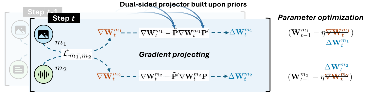
Figure 2: The paradigm of the proposed method for CMCL. At the current step $t$, gradients ($\nabla\mathbf{W}_{t}^{m_{1}}$ and $\nabla\mathbf{W}_{t}^{m_{1}}$) derived by contrastive learning between modalities $m_{1}$ and $m_{2}$ are projected from dual sides to $\Delta\mathbf{W}_{t}^{m_{1}}$ and $\Delta\mathbf{W}_{t}^{m_{1}}$. The projectors are built upon the features at the previous steps to constrain the gradients. By substituting for the gradients, model parameters are optimized from new modality pair data while retraining the prior knowledge.

Stability requirement. Recall the stability requirement in CMCL of $(\mathbf{Z}_{t-1;t}^{m_{1}})^{\top}\mathbf{Z}_{t-1;t}^{m_{2}}=\mathbf{A}^{m_{1},m_{2}}_{t-1;t-1}$: given the same modality pair data from the previous step, the model trained on new datasets should maintain the alignments on modality pairs from earlier steps. This implies that new updates (i.e., gradients) should not interfere with effective parts within the parameter space.

Plasticity requirement. According to the contrastive learning objective defined in Eq. (3), unconstrained gradients naturally encourage parameters optimized for previous datasets to adapt to new datasets. Thus, plasticity emerges directly from the inherent learning process. In vanilla CMCL, where the model sequentially trains on datasets without any explicit constraints, plasticity is inherently maintained. Introducing additional regularization strategies inherently increases risks to plasticity.

Theoretical motivation. Building upon the above analyses, we explore gradient updates in detail to establish theoretical motivations. Let us consider the left-hand side of Eq. (4), $(\mathbf{Z}_{t-1;t}^{m_{1}})^{\top}\mathbf{Z}_{t-1;t}^{m_{2}}$. We introduce the prior encoders of $g^{*}_{m}$ (cf., plasticity) and a linear operator that transfers the priors $\mathbf{Z}^{m_{1}}_{t-1;*}$ and $\mathbf{Z}^{m_{2}}_{t-1;*}$, with $\mathbf{Z}^{m_{1}}_{t-1;t}=\mathbf{W}^{m_{1}}_{t}\mathbf{Z}^{m_{1}}_{t-1;*}$ and $\mathbf{W}^{m_{1}}_{t}\in\mathbb{R}^{d\times d},{\mathbf{Z}^{m_{1}}_{t-1;*}\in\mathbb{R}^{d\times n}}$, where $d$ is the feature dimension and $n$ denotes the batch size. Besides, we consider the gradient update rule as $\mathbf{W}_{t}^{m}=\mathbf{W}_{t-1}^{m}-\eta\nabla\mathbf{W}_{t}^{m}$, where $\eta$ is the learning rate. Therefore, we have:

$$\quad(\mathbf{Z}_{t-1;t}^{m_{1}})^{\top}\mathbf{Z}_{t-1;t}^{m_{2}}$$ (5)

$$=(\mathbf{Z}^{m_{1}}_{t-1;*})^{\top}\underbrace{(\mathbf{W}^{m_{1}}_{t})^{\top}\mathbf{W}^{m_{2}}_{t}}_{\text{global parameters at step }t}\mathbf{Z}^{m_{2}}_{t-1;*}$$

$$=(\mathbf{Z}^{m_{1}}_{t-1;*})^{\top}{(\mathbf{W}^{m_{1}}_{t-1}-\eta\nabla\mathbf{W}_{t}^{m_{1}})^{\top}(\mathbf{W}^{m_{2}}_{t-1}}-\eta\nabla\mathbf{W}_{t}^{m_{2}})\mathbf{Z}^{m_{2}}_{t-1;*}$$

$$=(\mathbf{Z}^{m_{1}}_{t-1;*})^{\top}\underbrace{(\mathbf{W}^{m_{1}}_{t-1})^{\top}\mathbf{W}^{m_{2}}_{t-1}}_{\text{global parameters at step }t-1}\mathbf{Z}^{m_{2}}_{t-1;*}-\eta(\mathbf{Z}^{m_{1}}_{t-1;*})^{\top}\underbrace{\left((\mathbf{W}^{m_{1}}_{t-1})^{\top}\nabla\mathbf{W}^{m_{2}}_{t}+(\nabla\mathbf{W}^{m_{1}}_{t})^{\top}\mathbf{W}^{m_{2}}_{t-1}-\eta(\nabla\mathbf{W}^{m_{1}}_{t})^{\top}\nabla\mathbf{W}^{m_{2}}_{t}\right)}_{\text{updated global parameters }\tilde{\mathbf{W}}}\mathbf{Z}^{m_{2}}_{t-1;*}.$$

Projecting $\tilde{\mathbf{W}}$ (globally). We consider the parameter update globally, where $\tilde{\mathbf{W}}$ is used to update $(\mathbf{W}^{m_{1}}_{t-1})^{\top}\mathbf{W}^{m_{2}}_{t-1}$ via $(\mathbf{W}^{m_{1}}_{t})^{\top}\mathbf{W}^{m_{2}}_{t}=(\mathbf{W}^{m_{1}}_{t-1})^{\top}\mathbf{W}^{m_{2}}_{t-1}-\eta\tilde{\mathbf{W}}$. To keep stability for the previous datasets, we need to satisfy $(\mathbf{Z}^{m_{1}}_{t-1;*})^{\top}\tilde{\mathbf{W}}\mathbf{Z}^{m_{2}}_{t-1;*}=\mathbf{0}$. Therefore, $\mathbf{A}_{t-1;t}^{m_{1},m_{2}}=\mathbf{A}_{t-1;t-1}^{m_{1},m_{2}}+\mathbf{0}$.

Theorem 3.

Let the global parameter update follow $(\mathbf{W}_{t}^{m_{1}})^{\top}\mathbf{W}_{t}^{m_{2}}=(\mathbf{W}_{t-1}^{m_{1}})^{\top}\mathbf{W}_{t-1}^{m_{2}}-\eta\bar{\mathbf{W}}$, and the original parameter update be denoted as:

$$\tilde{\mathbf{W}}=\left((\mathbf{W}^{m_{1}}_{t-1})^{\top}\nabla\mathbf{W}^{m_{2}}_{t}+(\nabla\mathbf{W}^{m_{1}}_{t})^{\top}\mathbf{W}^{m_{2}}_{t-1}-\eta(\nabla\mathbf{W}^{m_{1}}_{t})^{\top}\nabla\mathbf{W}^{m_{2}}_{t}\right).$$ (6)

Then, the stability holds if

$$\bar{\mathbf{W}}:=\tilde{\mathbf{W}}-\mathbf{P^{\prime}}\tilde{\mathbf{W}}\mathbf{P},$$ (7)

where $\mathbf{P^{\prime}}$ and $\mathbf{P}$ are the space projectors for $\mathbf{Z}_{t-1;*}^{m_{1}}$ and $\mathbf{Z}_{t-1;*}^{m_{2}}$, respectively. See proof in Appendix B.1.

Projecting $\nabla\mathbf{W}$ (locally). Following this, we hope to update the local gradients in practice, i.e., optimizing the model parameters corresponding to each modality, to satisfy the stability. In the following, we find the deviation of the gradients close to the $\tilde{\mathbf{W}}-\mathbf{P^{\prime}}\tilde{\mathbf{W}}\mathbf{P}$ lies in the null space.

Theorem 4.

Let the local parameter update follow $\mathbf{W}_{t}^{m}=\mathbf{W}_{t-1}^{m}-\eta\Delta\mathbf{W}_{t}^{m}$, the stability holds if

$$\left\{\begin{aligned} \Delta\mathbf{W}_{t}^{m_{1}}&:=\nabla\mathbf{W}_{t}^{m_{1}}-\tilde{\mathbf{P}}\nabla\mathbf{W}_{t}^{m_{1}}\mathbf{P^{\prime}},\\ \Delta\mathbf{W}_{t}^{m_{2}}&:=\nabla\mathbf{W}_{t}^{m_{2}}-\tilde{\mathbf{P}}^{\prime}\nabla\mathbf{W}_{t}^{m_{2}}\mathbf{P},\end{aligned}\right.$$ (8)

where $\tilde{\mathbf{P}}^{\prime}$ and $\tilde{\mathbf{P}}$ are the space projectors for $\mathbf{Z}_{t-1;t-1}^{m_{1}}$ and $\mathbf{Z}_{t-1;t-1}^{m_{2}}$, respectively. See proof in Appendix B.2.

3.3 The Theoretical Guarantee: Bounds and Capabilities

After inferring the method to achieve CMCL, we examine the performance guarantees theoretically. Besides, we introduce the extensions for any steps and any modality pairs during the practical training procedure.

Theorem 5 (The upper bound of loss of stability).

In CMCL, the upper bound of loss of stability is:

$$\|\mathbf{A}^{m_{1},m_{2}}_{t-1;t}-\mathbf{A}^{m_{1},m_{2}}_{t-1;t-1}\|_{2}\leq\eta^{2}\cdot\|\mathbf{Z}^{m_{1}}_{t-1;*}\|_{2}\|\mathbf{Z}^{m_{2}}_{t-1;*}\|_{2}\cdot\mathcal{F}(\nabla\mathbf{W}),$$ (9)

where $\mathcal{F}$ represents the interactions between different updated gradients $\nabla\mathbf{W}_{t}^{m_{1}}$ and $\nabla\mathbf{W}_{t}^{m_{2}}$. Specifically, $\mathcal{F}(\nabla\mathbf{W}):=2\|\nabla\mathbf{W}^{m_{1}}_{t}\|_{2}\|\nabla\mathbf{W}^{m_{2}}_{t}\|_{2}+\|\nabla\mathbf{W}^{m_{1}}_{t}\|^{2}_{2}+\|\nabla\mathbf{W}^{m_{2}}_{t}\|^{2}_{2}$. See proof in Appendix B.3.

Theorem 6 (The upper bound of plasticity).

By transforming the gradients, the loss $\mathcal{L}_{t}$ update at step $t$ from the previous loss $\mathcal{L}_{t-1}$ is following:

$$\mathcal{L}_{t}-\mathcal{L}_{t-1}\leq 0$$ (10)

to keep the plasticity when $\frac{o(\eta)}{\eta}\leq 0$ at the time $t$. See proof in Appendix B.4.

Extension for any steps $\{\mathbf{A}^{m,m^{\prime}}_{i;*}\}_{<t}$. In general, on continual learning, we hope to maintain stability for any seen datasets. Hence, we have:

$${\textbf{A}^{m_{1},m_{2}}_{i;t}}={\textbf{A}^{m_{1},m_{2}}_{i;i}},\quad\forall i<t.$$ (11)

That means we need to project $\tilde{\mathbf{W}}$ onto the null space of all previous datasets, via $\mathbf{P}_{<t}$. We utilize the uncentered feature covariance [17] to obtain the null space projector via SVD approximation (Section 2). Let $\bar{\mathbf{Z}}^{m}_{<t}=\frac{\bar{n}_{t-2}}{\bar{n}_{t-1}}\bar{\mathbf{Z}}^{m}_{<t-1}+\frac{{n}_{t-1}}{\bar{n}_{t-1}}\tilde{\mathbf{Z}}^{m}_{t-1}$, where $\tilde{\mathbf{Z}}^{m}_{t-1}\triangleq\frac{1}{n_{t-1}}(\mathbf{Z}^{m}_{t-1})^{\top}\mathbf{Z}^{m}_{t-1}$ (the equality is proved in Appendix B.5). Similarly, for local gradient updates, $\mathbf{\Delta}:=\mathbf{P^{\prime}}_{<t}\tilde{\mathbf{W}}\mathbf{P}_{<t}$ for extension. For the local gradient update, we are required to maintain an additional feature covariance constructed from the previous models. We can achieve this in efficiency. For instance, $\Delta\mathbf{W}_{t}^{m_{2}}:=\nabla\mathbf{W}_{t}^{m_{2}}-\tilde{\mathbf{P}}^{\prime}\nabla\mathbf{W}_{t}^{m_{2}}\mathbf{P}$, where $\tilde{\mathbf{P}}^{\prime}$ is the space projector for $\mathbf{Z}_{t-1;t-1}^{m_{1}}$. Note that, the guarantee for stability and plasticity can be easily extended to any step, as we only modify the projectors that are able to project the features onto the space that covers all previous datasets.

Extension for any modality pairs $\{m,m^{\prime}\}_{<t}$. In particular, on CMCL, diverse modality pairs are involved to optimize corresponding encoders. In this case, we can simply extend the previous gradient update on $\{m_{1},m_{2}\}$ in step $t-1$ and $t$ to any different adjacent modality pairs. Assume training on modality pairs of $\{m_{1},m_{2}\}$ at step $t-1$ and $\{m_{1},m_{3}\}$ at step $t$, if $m_{3}:=m_{2}$, it follows Theorem 4. If $m_{3}\neq m_{2}$, we can set $\nabla\mathbf{W}_{t}^{m_{3}}=\mathbf{0}$. Furthermore, the corresponding feature projector update can be omitted as well to save computational cost. Therefore, only features at relevant steps are required to be updated rather than considering all steps. The algorithm flow and pseudo-code are provided in Appendix A.1.

Table 1: The statistics of datasets for modality pair training, which involve modalities of V$\leftrightarrow$Vision, A$\leftrightarrow$Audio, T$\leftrightarrow$Text, VI$\leftrightarrow$VIdeo, TH$\leftrightarrow$THermal, TA$\leftrightarrow$TActile, and D$\leftrightarrow$Depth.

Dataset	Modalities							Evaluation	Tasks		Modes	#Examples	#Classes
	V	A	T	VI	TH	TA	D		Retrieval	Classification
UCF101	-	-	✓	✓	-	-	-	Acc	-	✓	Train, Test	8,080	101
ESC50	-	✓	✓	-	-	-	-	Recall, Acc	✓	✓	Train, Test	2,000	50
NYUDv2	✓	-	-	-	-	-	✓	Recall	✓	-	Train, Test	48,238	-
VGGSound-S	-	✓	✓	✓	-	-	-	Recall, Acc	✓	✓	Train, Test	12,000	309
Clotho	-	✓	✓	-	-	-	-	Recall	✓	-	Train, Test	4,885	-
TVL	✓	-	✓	-	-	✓	-	Recall	✓	-	Train, Test	43,741	-
LLVIP	✓	-	-	-	✓	-	-	Recall	✓	-	Train, Test	15,488	-

4 Experiments

4.1 Experimental Setups

Tasks & datasets. We evaluate on 7 multimodal datasets, including UCF101 [28], ESC50 [29], NYUDv2 [30], VGGSound-S [31], Clotho [32], TVL [33], and LLVIP [34]. For performance comparison, we mainly categorize the evaluation tasks as retrieval and classification. The important statistics are provided in Table 1. More details are provided in Appendix A.2. For datasets with more than two modalities, we split them into bi-modal ones to cater to the modality pair training. For instance, VGGSound-S will be reorganized into three versions (VI-A, VI-A, and T-A). As a result, 11 training steps are involved in our training and evaluation.

Implementation details. We utilize pre-trained modality-binding methods as priors, followed by linear learners for each modality for training. Specifically, we employ ImageBind [12], LanguageBind [16], and UniBind [14], which are already trained with a sequence of modality pairs and are capable of generating multimodal representations in a joint space. Upon these powerful priors, we construct the projection module that projects the novel knowledge onto the dual-side null space of the previous one within the trainable parameters. We utilize PyTorch [35] for implementation. The model is optimized via an AdamW optimizer [36] with a learning rate of 0.0001 and weight decay of 0.001. The batch size is set to 64. We approximate the null space projection with truncated SVD, where a minimum eigenvalue $\lambda_{\min}$ is set to 0.01 for ImageBind and Unibind, while 0.0001 for LanguageBind. See more implementation details in Appendix A.3 and A.5.

Baselines. We consider various methods from continual learning fields. Specifically, we select Vanilla (continual training without any strategy) [12], Gradient Episodic Memory (GEM) [37], Dark Experience Replay (DER & DER++) [38], Elastic Weight Consolidation (EWC) [39], Contrastive Continual Learning (Co²L) [18], C-Flat [40], and Contrastive Incremental Learning with Adaptive distillation (CILA) [19]. Notably, our method is replay-free, which maintains efficiency. We adapt these methods for the CMCL setting. More details of the baselines are provided in Appendix A.4.

Evaluation metrics. We consider the evaluation metrics from both consistency (learnability) and determinism (anti-forgetting) perspectives. For consistency, we employ Recall@$k$ for cross-modal retrieval tasks, where $k$ is set in the range of $\{1,5,10\}$. Besides, we use average accuracy (Acc) for classification tasks. For determinism, we employ backward transfer (BWT), which computes the average drop of performance at the previous step after learning the current dataset. In this case, higher appearance scores of these metrics indicate higher consistency and determinism. More details of the metrics can be checked in Appendix A.5.

Table 2: Average performance (mean$\pm$std.) on classification and retrieval tasks. Here “R@$k$” is the abbreviation of “Recall@$k$”. The results are calculated over ten independent trials. The best result in each case is marked as bold.

Method		Classification		Retrieval
		Acc	BWT${}_{\text{A}}$	R@1	R@5	R@10	BWT${}_{\text{R10}}$
ImageBind	Vanilla	47.32$\ {\pm 0.27}$	-5.72$\ {\pm 0.44}$	9.93$\ {\pm 0.09}$	27.86$\ {\pm 0.18}$	38.56$\ {\pm 0.14}$	-3.34$\ {\pm 0.09}$
	GEM	40.98$\ {\pm 1.65}$	-9.75$\ {\pm 1.64}$	9.53$\ {\pm 0.14}$	27.00$\ {\pm 0.28}$	37.38$\ {\pm 0.31}$	-2.91$\ {\pm 0.26}$
	DER	47.34$\ {\pm 0.41}$	-5.70$\ {\pm 0.54}$	9.91$\ {\pm 0.08}$	27.88$\ {\pm 0.18}$	38.55$\ {\pm 0.20}$	-3.32$\ {\pm 0.08}$
	DER++	47.40$\ {\pm 0.15}$	-4.71$\ {\pm 0.48}$	9.94$\ {\pm 0.12}$	27.95$\ {\pm 0.18}$	38.72$\ {\pm 0.13}$	-3.09$\ {\pm 0.11}$
	EWC	48.34$\ {\pm 1.53}$	-4.82$\ {\pm 1.18}$	10.07$\ {\pm 0.24}$	28.35$\ {\pm 0.55}$	39.22$\ {\pm 0.69}$	-2.55$\ {\pm 0.76}$
	Co2L	50.13$\ {\pm 0.52}$	-3.74$\ {\pm 0.51}$	9.79$\ {\pm 0.04}$	27.99$\ {\pm 0.21}$	38.66$\ {\pm 0.23}$	-1.77$\ {\pm 0.19}$
	C-FLAT	50.96$\ {\pm 0.34}$	-4.17$\ {\pm 0.48}$	9.92$\ {\pm 0.09}$	28.90$\ {\pm 0.14}$	39.97$\ {\pm 0.19}$	-1.41$\ {\pm 0.19}$
	CILA	50.73$\ {\pm 0.48}$	-3.20$\ {\pm 0.74}$	9.68$\ {\pm 0.11}$	27.76$\ {\pm 0.20}$	38.25$\ {\pm 0.20}$	-1.28$\ {\pm 0.21}$
	DNS (ours)	52.52$\ {\pm 0.23}$	-0.02$\ {\pm 0.30}$	10.38$\ {\pm 0.09}$	29.53$\ {\pm 0.17}$	40.89$\ {\pm 0.10}$	-1.07$\ {\pm 0.12}$
LanguageBind	Vanilla	51.86$\ {\pm 1.13}$	-15.71$\ {\pm 1.22}$	7.51$\ {\pm 0.10}$	25.36$\ {\pm 0.32}$	36.02$\ {\pm 0.49}$	-10.19$\ {\pm 0.53}$
	GEM	60.15$\ {\pm 0.63}$	-4.98$\ {\pm 0.52}$	8.32$\ {\pm 0.13}$	28.92$\ {\pm 0.14}$	41.24$\ {\pm 0.22}$	-4.12$\ {\pm 0.18}$
	DER	52.55$\ {\pm 1.08}$	-14.96$\ {\pm 0.88}$	7.55$\ {\pm 0.16}$	25.47$\ {\pm 0.36}$	36.08$\ {\pm 0.46}$	-10.11$\ {\pm 0.46}$
	DER++	55.86$\ {\pm 1.64}$	-10.45$\ {\pm 1.58}$	7.33$\ {\pm 0.20}$	25.66$\ {\pm 0.53}$	36.50$\ {\pm 0.61}$	-9.58$\ {\pm 0.62}$
	EWC	54.03$\ {\pm 1.94}$	-13.45$\ {\pm 2.34}$	8.00$\ {\pm 0.26}$	27.11$\ {\pm 0.92}$	38.14$\ {\pm 1.26}$	-7.71$\ {\pm 1.44}$
	Co2L	58.08$\ {\pm 0.64}$	-5.79$\ {\pm 1.22}$	8.33$\ {\pm 0.12}$	28.33$\ {\pm 0.24}$	40.15$\ {\pm 0.31}$	-3.92$\ {\pm 0.37}$
	C-FLAT	57.84$\ {\pm 0.75}$	-7.57$\ {\pm 0.92}$	8.23$\ {\pm 0.10}$	28.02$\ {\pm 0.17}$	39.72$\ {\pm 0.25}$	-5.00$\ {\pm 0.32}$
	CILA	59.30$\ {\pm 0.62}$	-2.63$\ {\pm 0.91}$	8.32$\ {\pm 0.14}$	28.31$\ {\pm 0.26}$	40.48$\ {\pm 0.27}$	-1.09$\ {\pm 0.40}$
	DNS (ours)	64.07$\ {\pm 0.37}$	-0.09$\ {\pm 0.59}$	8.71$\ {\pm 0.06}$	29.81$\ {\pm 0.23}$	42.44$\ {\pm 0.20}$	-3.00$\ {\pm 0.21}$
UniBind	Vanilla	47.48$\ {\pm 0.56}$	-5.46$\ {\pm 0.61}$	10.09$\ {\pm 0.10}$	28.16$\ {\pm 0.26}$	38.93$\ {\pm 0.24}$	-3.52$\ {\pm 0.20}$
	GEM	41.37$\ {\pm 1.52}$	-9.29$\ {\pm 1.20}$	9.61$\ {\pm 0.14}$	27.32$\ {\pm 0.31}$	37.94$\ {\pm 0.34}$	-2.97$\ {\pm 0.39}$
	DER	47.64$\ {\pm 0.57}$	-5.35$\ {\pm 0.65}$	10.10$\ {\pm 0.09}$	28.16$\ {\pm 0.25}$	38.95$\ {\pm 0.26}$	-3.51$\ {\pm 0.20}$
	DER++	47.75$\ {\pm 0.23}$	-4.69$\ {\pm 0.71}$	10.06$\ {\pm 0.08}$	28.30$\ {\pm 0.21}$	39.10$\ {\pm 0.15}$	-3.39$\ {\pm 0.12}$
	EWC	48.21$\ {\pm 1.48}$	-5.06$\ {\pm 1.19}$	10.24$\ {\pm 0.25}$	28.60$\ {\pm 0.54}$	39.47$\ {\pm 0.66}$	-2.89$\ {\pm 0.67}$
	Co2L	50.45$\ {\pm 0.59}$	-3.47$\ {\pm 0.92}$	9.87$\ {\pm 0.08}$	28.30$\ {\pm 0.16}$	39.21$\ {\pm 0.20}$	-1.87$\ {\pm 0.21}$
	C-FLAT	51.25$\ {\pm 0.42}$	-4.36$\ {\pm 0.49}$	10.00$\ {\pm 0.06}$	29.19$\ {\pm 0.17}$	40.51$\ {\pm 0.12}$	-1.48$\ {\pm 0.18}$
	CILA	51.03$\ {\pm 0.41}$	-2.93$\ {\pm 0.75}$	9.76$\ {\pm 0.08}$	28.07$\ {\pm 0.14}$	38.80$\ {\pm 0.17}$	-1.40$\ {\pm 0.20}$
	DNS (ours)	52.86$\ {\pm 0.29}$	0.31$\ {\pm 0.46}$	10.52$\ {\pm 0.06}$	29.97$\ {\pm 0.10}$	41.44$\ {\pm 0.11}$	-1.19$\ {\pm 0.12}$

4.2 Results

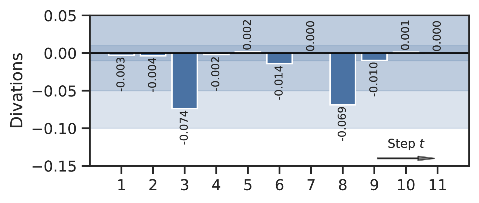
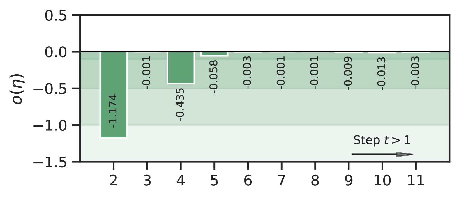
(a)

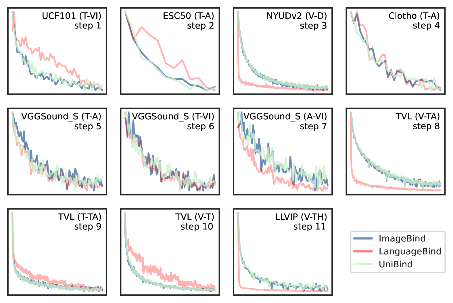
(b)

Figure 3: (a) The illustrations on stability and plasticity: the top showcases deviations between $\mathbf{A}_{N;t-1}$ (bars) and $\mathbf{A}_{t-1;t-1}$ (middle line); the bottom represents the average of high-order terms at each steps $t>1$. (b) The curves plot batch-wise training losses.

Overall evaluation. We compare our method (DNS) with selected baselines on both classification and retrieval tasks with results being reported in Table 2. This result demonstrates that DNS outperforms all baselines on two types of performance metrics (i.e., Acc and Recall). Particularly in the classification task, DNS (ours) consistently achieves the highest accuracy and exhibits minimal or even positive BWT${}_{\text{A}}$, whereas other methods generally suffer from higher negative transfer. In the retrieval task, DNS outperforms other methods in all Recall@$k$ (R@1, R@5, and R@10) metrics, and it also demonstrates good backward transfer ability. These results highlight the effectiveness of DNS in mitigating catastrophic forgetting (stability) and achieving superior performance (plasticity) across both classification and retrieval tasks.

Stability analyses. To test the stability defined in Eq. (4), we compare the alignment scores from two sides. At each step, we average the scores of modality pairs, which will be compared at subsequent steps, with the results shown in Figure 3(a). We can observe that the deviations are small and even reach nearly zero at some steps, further sustaining the stability maintaining of DNS.

Plasticity analyses. We provide empirical support corresponding to the theoretical insights on plasticity in Theorem 6. Specifically, we compute the high-order term and verify whether it satisfies $\frac{o(\eta)}{\eta}\leq 0$. We report the results in Figure 3(a) and have the following observations. At each step $t>1$, the averaged $o(\eta)$ is negative and near to 0, which confirms our claim in Theorem 6 in a practical scenario. Furthermore, the training loss converging supports the plasticity as well, in Section 4.3.

4.3 More Analyses and Justifications

Training loss curves. We evaluate the stability and plasticity through training losses over batches. The batch-wise training loss illustrates the learning status at the own step (plasticity). The results are showcased in Figure 3(b). From the observation, our method can achieve a stable training loss even after the model is optimized by new datasets and the batch-wise loss also successfully converges. These findings demonstrate DNS reaches a balance between stability and plasticity.

Table 3: The time recording (s) for vanilla, replay (DER), and DNS training for one step.

	Vanilla	Replay-based	DNS
ImageBind	32.35	547.42	36.51 (0.52)
LanguageBind	31.89	541.53	33.77 (0.46)
UniBind	34.10	543.67	36.05 (0.81)

Efficiency analyses. DNS maintains efficiency for CMCL, which differs from replay-based methods that require additional buffer memory and further introduce more computational costs. Here we evaluate the efficiency of our methods by recording the time in training, as shown in Table 3. The replay-based method requires more training time compared to both the vanilla method and DNS. DNS introduces a slight increase in training time due to the gradient projection and SVD approximation (detailed in parentheses), while still preserving overall training efficiency.

5 Conclusion and Discussion

In this paper, we introduce and formally define Continual Multimodal Contrastive Learning (CMCL), a research question on how to incrementally integrate multimodal data through contrastive learning. We specify the definitions of stability and plasticity in CMCL. Theoretically, we derive a novel method, termed DNS, which employs a dual-sided gradient-projection strategy to balance the incorporation of new modality pairs while preserving existing multimodal knowledge effectively. The parameter gradients are projected from one side of its own modality and another side of the interacted modalities onto subspaces. Any newly-projected gradient within these subspaces makes no effect to the prior effective parameter spaces. Furthermore, two upper bounds are provided with theoretical insights on both stability and plasticity and support the effectiveness of our gradient-projection method. Empirical results across seven datasets demonstrate our method’s superiority over current state-of-the-art continual learning baselines, which confirms both its robustness and efficiency.

The CMCL framework holds significant potential for applications in complex fields like medicine and neuroscience, where modalities such as MRI, CT scans, and electrophysiological signals require incremental integration. In medical diagnostics, CMCL can incrementally incorporate diverse imaging modalities. In neuroscience research, our framework can facilitate the progressive understanding of neural correlates by continually integrating modalities like functional MRI, EEG, and MEG, thereby providing richer insights into brain functions and disorders. CMCL presents an exciting avenue for future interdisciplinary research to enhance both interpretability and performance.

Appendix A Implementation Details

A.1 Training and Inference Procedures

Here we provide the training algorithm flow in Algorithm 1 and the corresponding pseudo-code. The inference algorithm flow is demonstrated in Algorithm 2. Algorithm 1 describes the Continual Multimodal Contrastive Learning training process with our method DNS, which enables a model to progressively learn from new multimodal data while maintaining stability in previously learned modality alignments.

Algorithm 1 DNS for Continual Multimodal Contrastive Learning (Training)

0: Inputs:    Pre-trained encoders $\{g^{*}_{m}\}_{m\in\mathcal{M}}$ and follow-up learner $\{\mathbf{W}^{m}\}_{m\in\mathcal{M}}$ for each modality $m$, learning rate $\eta$,    A sequence of training datasets $\{\mathcal{X}^{m,m^{\prime}}_{t}\}_{t=1}^{N}$, each containing modality pairs.    Feature covariance matrix $\{\bar{\mathbf{Z}}_{<t;*}^{m}\}_{m\in\mathcal{M}}$ and $\{\bar{\mathbf{Z}}_{<t;<t}^{m}\}_{m\in\mathcal{M}}$ (initially $t=1$).

0: Updated model parameters $\{\mathbf{W}_{t}^{m}\}$ (i.e., $\{\mathbf{\theta}_{m}^{t}\}$) that preserve alignment stability on previously seen data.

1: Initialize features covariance storages $\{\bar{\mathbf{Z}}_{<t;*}^{m}\}_{m\in\mathcal{M}}$ and $\{\bar{\mathbf{Z}}_{<t;<t}^{m}\}_{m\in\mathcal{M}}$ to zero.

2: Initialize local parameters from $\{\mathbf{W}^{m}\}_{m\in\mathcal{M}}$.

3: for $t=1$ to $N$ do

4:  Prior to the new step $\{m,m^{\prime}\}$:

5:   ① Retrieve feature variance $\{\bar{\mathbf{Z}}_{<t;*}^{m}\}_{m\in\{m,m^{\prime}\}}$ and $\{\bar{\mathbf{Z}}_{<t;<t}^{m}\}_{m\in\{m,m^{\prime}\}}$.

6:   ② Compute the projectors:

7:   

$$\mathbf{P}_{<t}\leftarrow\bar{\mathbf{Z}}_{<t;*}^{m},\quad\tilde{\mathbf{P}}_{<t}\leftarrow\bar{\mathbf{Z}}_{<t;<t}^{m},\quad\mathbf{P^{\prime}}_{<t}\leftarrow\bar{\mathbf{Z}}_{<t;*}^{m^{\prime}},\quad\tilde{\mathbf{P^{\prime}}}_{<t}\leftarrow\bar{\mathbf{Z}}_{<t;<t}^{m^{\prime}}$$

8:  Train on the new dataset $\mathcal{X}^{m,m^{\prime}}_{t}$:

9:   Repeat until convergence:

10:    ① Sample a mini-batch $\{(\mathbf{x}^{m},\mathbf{x}^{m^{\prime}})\}$ from $\mathcal{X}^{m,m^{\prime}}_{t}$.

11:    ② Compute representations and the multimodal contrastive loss:

$$\mathcal{L}_{m,m^{\prime}}=\mathcal{L}\bigl{(}g_{m}(\mathbf{x}^{m};\mathbf{W}_{t-1}^{m}),\;g_{m^{\prime}}(\mathbf{x}^{m^{\prime}};\mathbf{W}_{t-1}^{m^{\prime}})\bigr{)}.$$

12:    ③ Compute the raw gradients:

$$\nabla\mathbf{W}_{t}^{m}\leftarrow\frac{\partial\mathcal{L}_{m,m^{\prime}}}{\partial\mathbf{W}_{t-1}^{m}},\quad\nabla\mathbf{W}_{t}^{m^{\prime}}\leftarrow\frac{\partial\mathcal{L}_{m,m^{\prime}}}{\partial\mathbf{W}_{t-1}^{m^{\prime}}}.$$

13:    ④ Project the gradients so that old alignments are preserved (Theorem 4):

$$\Delta\mathbf{W}_{t}^{m}\;\;=\;\;\nabla\mathbf{W}_{t}^{m}\;-\;\tilde{\mathbf{P}}_{<t}\,\nabla\mathbf{W}_{t}^{m}\,\mathbf{P}^{\prime}_{<t},$$

$$\Delta\mathbf{W}_{t}^{m^{\prime}}\;\;=\;\;\nabla\mathbf{W}_{t}^{m}\;-\;\tilde{\mathbf{P}}^{\prime}_{<t}\,\nabla\mathbf{W}_{t}^{m}\,\mathbf{P}_{<t},$$

14:    ⑤ Update the parameters:

$$\mathbf{W}_{t}^{m}\;\leftarrow\;\mathbf{W}_{t-1}^{m}\;-\;\eta\,\Delta\mathbf{W}_{t}^{m},\quad\mathbf{W}_{t}^{m^{\prime}}\;\leftarrow\;\mathbf{W}_{t-1}^{m^{\prime}}\;-\;\eta\,\Delta\mathbf{W}_{t}^{m^{\prime}}.$$

15:   End mini-batch.

16:  Update the feature covariances (step-wise or batch-wise):

17:   $\bar{\mathbf{Z}}^{m}_{<t+1;*}=\frac{\bar{n}_{t-1}}{\bar{n}_{t}}\bar{\mathbf{Z}}^{m}_{<t;*}+\frac{1}{\bar{n}_{t}}(\mathbf{Z}^{m}_{t;*})^{\top}\mathbf{Z}^{m}_{t;*}$,  $\bar{\mathbf{Z}}^{m}_{<t+1;<t+1}=\frac{\bar{n}_{t-1}}{\bar{n}_{t}}\bar{\mathbf{Z}}^{m^{\prime}}_{<t;<t}+\frac{1}{\bar{n}_{t}}(\mathbf{Z}^{m^{\prime}}_{t;t})^{\top}\mathbf{Z}^{m^{\prime}}_{t;t}$,

18:   $\bar{\mathbf{Z}}^{m^{\prime}}_{<t+1;*}=\frac{\bar{n}_{t-1}}{\bar{n}_{t}}\bar{\mathbf{Z}}^{m^{\prime}}_{<t;*}+\frac{1}{\bar{n}_{t}}(\mathbf{Z}^{m^{\prime}}_{t;*})^{\top}\mathbf{Z}^{m^{\prime}}_{t;*}$,  $\bar{\mathbf{Z}}^{m^{\prime}}_{<t+1;<t+1}=\frac{\bar{n}_{t-1}}{\bar{n}_{t}}\bar{\mathbf{Z}}^{m}_{<t;<t}+\frac{1}{\bar{n}_{t}}(\mathbf{Z}^{m}_{t;t})^{\top}\mathbf{Z}^{m}_{t;t}$.

19:   

20: end for

21: Return: $\{\mathbf{W}_{N}^{m}\}$ preserving stability for all previously learned pairs $(m,m^{\prime})$.

DNS provides a convenient way to modify gradients before the optimizer step. By applying structured transformations using precomputed projection matrices, it ensures better optimization while keeping the implementation modular and flexible. The pseudo-code for gradient updates is shown below.

Algorithm 2 describes the inference process for Continual Multimodal Contrastive Learning. The goal is to perform inference on a given test sample from a specific modality and generate aligned representations.

Algorithm 2 DNS for Continual Multimodal Contrastive Learning (Inference)

0: Inputs:    Pre-trained encoders $\{g^{*}_{m}\}_{m\in\mathcal{M}}$ and trained learner $\{\mathbf{W}^{m}\}_{m\in\mathcal{M}}$ for each modality $m$,    A test sample (or a query) in modality $m$, denoted $\mathbf{x}^{m}$.

0:  Inference outputs (e.g., aligned representations, retrieval scores).

1: Obtain representation:

$$\mathbf{z}^{m}=\mathbf{W}_{N}^{m}g_{m}\bigl{(}\mathbf{x}^{m}\bigr{)},\quad\mathbf{z}^{m^{\prime}}=\mathbf{W}_{N}^{m^{\prime}}g_{m^{\prime}}\bigl{(}\mathbf{x}^{m^{\prime}}\bigr{)}.$$

2: Perform downstream task:

3:  For example, retrieve the best match in another modality $m^{\prime}$ via

$$\max_{\mathbf{z}^{m^{\prime}}}\;(\mathbf{z}^{m})^{\top}\mathbf{z}^{m^{\prime}}\quad\text{(or apply other alignment criteria)}.$$

4: Output the alignment scores, predicted labels, or retrieved results, etc.

A.2 Datasets

Below, we introduce the used datasets in more detail.

• UCF101 [28] is a widely used dataset for action recognition across 101 action categories, sourced from YouTube. It extends the UCF50 dataset, introducing greater diversity and real-world complexity with significant variations in camera motion, object appearance, viewpoint, background clutter, and illumination. The 101 action categories span 5 broad types: 1) Human-Object Interaction (e.g., cutting in kitchen); 2) Body-Motion Only (e.g., jump rope and Tai Chi); 3) Human-Human Interaction (e.g., boxing and head massage); 4) Playing Musical Instruments (e.g., playing violin and playing tabla); 5) Sports (e.g., basketball dunk and pole vault). In our case, we select 70 examples for each category for training, and 10 examples for each category for testing to balance the distribution.

• ESC50 [29] is a collection of 2,000 five-second environmental audio recordings, designed for benchmarking methods in environmental sound classification. It consists of 50 semantically distinct classes, each containing 40 examples, grouped into 5 major categories: 1) Animals (e.g., dog, cat, and frog); 2) Natural Soundscapes & Water Sounds (e.g., rain, sea waves, and thunderstorm); 3) Human Non-Speech Sounds (e.g., laughing, sneezing, and footsteps); 4) Interior/Domestic Sounds (e.g., door knock, washing machine, and clock alarm); 5) Exterior/Urban Noises (e.g., car horn, airplane, and fireworks). All clips have been manually extracted from public field recordings available on Freesound.org. To evaluate the performance, we randomly split the data with a ratio of 4:1 for training (1,600) and testing (400).

• NYUDv2 [30, 41] is a dataset originally for depth estimation and semantic segmentation, which features video sequences of indoor scenes captured with both RGB and depth cameras from Microsoft Kinect. We use the preprocessed version of the original NYU Depth V2 dataset linked above. It is also used in the TensorFlow dataset. In this version, 47,584 examples are used for training, and 654 examples are for testing.

• VGGSound-S [31] is extracted from content-sharing platform, YouTube, consisting of short clips of audio sounds. It consists of 10-second video segments collected “in the wild”, which ensures that the sound source is visually evident in each clip. The dataset spans a wide range of acoustic environments and diverse noise conditions, making it highly representative of real-world applications. To facilitate the training and evaluation, we downsample a small version of VGGSound, namely VGGSound-S, which consists of 10,000 examples for training and 2,000 examples for testing.

• Clotho [32] is an audio captioning dataset, with all audio examples being from the Freesound platform. The duration of the audio is in the range of 15 to 30 seconds. Each audio has captions up to 20 words in length, collected by AMT or a specific protocol for crowd-sourcing audio annotations. We only keep one caption per audio in our case and use its development set (3,840) for training and evaluation set (1,045) for testing.

• TVL [33] is a large-scale image-touch dataset designed for multimodal learning, combining two datasets: 1) SSVTP [42], a robot-collected dataset with 4,587 image-touch pairs, manually labeled with image annotations; and 2) HCT, a large-scale dataset with 39,154 synchronously captured in-the-wild image-touch pairs, labeled using GPT-4V [43] based on visual inputs. We use its provided split for training and testing.

• LLVIP [34] is a visible-infrared paired dataset designed for low-light vision applications, which contains 30,976 images (15,488 pairs) captured in extremely dark scenes. All images are strictly aligned in time and space. We also use its default split for training and testing.

A.3 Modality-Binding Methods

Table 4: Details of different modality-binding methods, which include the supported modalities (V$\leftrightarrow$Vision, T$\leftrightarrow$Text, VI$\leftrightarrow$VIdeo, A$\leftrightarrow$Audio, D$\leftrightarrow$Depth, TH$\leftrightarrow$THermal, IMU$\leftrightarrow$Inertial Measurement Unit, EV$\leftrightarrow$EVent, and P$\leftrightarrow$Point cloud), feature dimension, and the number of datasets for pre-training.

	Modalities	Feature dimension	#Datasets
ImageBind	V, T, VI, A, D, TH, IMU	1,024	4
LanguageBind	V, T, VI, A, D, TH	768	6
UniBind	V, T, VI, A, TH, EV, P	1,024	13

Here we introduce three modality-binding methods used in this work (also check the details in Table 4).

• ImageBind [12] aligns six modalities, i.e., images, text, audio, depth, thermal, and IMU, into a joint embedding space, with vision-relevant modality pair data. It utilizes 4 datasets, containing video-audio (Audioset [44]), image-depth (SUN RGB-D [45]), image-thermal (LLVIP [34]), and video-IMU (Ego4D [46]), for pre-training.

• LanguageBind [16] takes language (i.e., text) as the bind across different modalities, including video, infrared, depth, audio and text. Languagebind is pre-trained on the collected dataset VIDAL-10M [16], which is extracted from 6 datasets: YouTube-8M [47], MSR-VTT [48], COCO [49], AVA [50], HMDB-51 [51], and ImageNet [52].

• UniBind [14] learns a unified and balanced representation space with large language models (LLMs) for data augmentation. All modality embeddings are aligned with the embedding centers yielded from LLM-augmented data. 1,000 descriptions for each category are generated via LLMs (GPT-4 [43] and LLaMA [53]), and multimodal data descriptions are obtained by multimodal LLMs like BLIP2 [54] and LLaMA-Adapter [55].

A.4 Baselines

Below, we discuss the used baselines in more detail.

• GEM [37] utilizes an episodic memory to store observed examples for each task. GEM computes gradients on the current task and compares them to gradients on the stored episodic memory. The inner product between these loss gradient vectors is assumed to be positive ($\langle\nabla_{t},\nabla_{k}\rangle\geq 0,\forall k<t$) so that the proposed parameter update $\nabla_{t}$ is unlikely to increase the loss at the previous tasks.

• DER & DER++ [38] maintain the network’s logits from the past tasks with being compared to the logits at the current task. In particular, DER++ further introduces the ground-truth labels serving as an additional regularization to stabilize the optimization. In our case, since we do not have explicit labels, we directly use a binary class to determine whether the modality pairs are from the same instance.

• EWC [39] utilizes the Fisher information matrix to estimate the importance of each parameter from previous tasks. Besides, EWC penalizes significant deviations from previous optimal values. As a result, it adds a quadratic constraint term to the loss function. The posterior is approximated as a Gaussian distribution and resolved via a Laplace approximation.

• Co²L [18] is a replay-based continual contrastive learning method. In more detail, Co²L modifies the supervised contrastive loss by viewing the examples within current tasks as the anchor, while examples at past tasks as the negatives. The instance-wise relations from the previous model are distilled to preserve the learned knowledge. Therefore, two objectives are combined with a controllable hyperparameter for the optimization of model parameters.

• C-FLAT [40] introduces an optimization method to enhance the existing continual learning method by promoting loss landscape flatness. It incorporates zeroth-order and first-order sharpness-aware optimization, balancing both local minima selection and landscape smoothness. C-FLAT is also encapsulated as a “plug-and-play” optimizer. In our case, we implement this method built upon Co²L.

• CILA [19] decomposes the continual learning objective into two components: a supervised contrastive loss and a distillation loss, following Co²L. In particular, CILA introduces an adaptive distillation induced by theoretical analyses. The distillation coefficients are dynamically updated based on the ratio of past distillation and contrastive losses.

We implement these methods following public repositories like mammoth, Co2L, and GradientEpisodicMemory.

A.5 Evaluation Settings

Evaluation metrics. We use $\text{Recall@}k$, Acc, and BWT for retrieval and classification tasks. BWT indicates the anti-forgetting capability. $\text{Recall@}k$ measures the ability of a model to retrieve the correct item among the top-$k$ candidates. Formally, for a dataset with $n$ queries, $\text{Recall@}k$ is defined as:

$$\text{Recall@}k:=\frac{1}{n}\sum_{i=1}^{n}\mathbb{I}(r(i)\leq k),$$ (12)

where $\mathbb{I}(\cdot)$ is the indicator function that returns 1 if the condition is true and 0 otherwise; $r(\cdot)$ denotes the position of the ground truth item for the $i$-th query in the ranked retrieval list. For classification tasks, average accuracy (Acc) is employed to measure the proportion of correctly predicted labels. Specifically, given the ground-truth label $y_{i}$ and the predicted label $\hat{y}_{i}$ for each instance in datasets with size of $n$, accuracy is given by:

$$\text{Acc}:=\frac{1}{n}\sum_{i=1}^{n}\mathbb{I}(y_{i}=\hat{y}_{i}).$$ (13)

Here $\hat{y}_{i}$ is calculated by finding the closest categories vectors with the query vector, i.e., $(\mathbf{z}_{i}^{m})^{\top}\mathbf{z}^{\text{T}}_{c}$, where $\mathbf{z}^{\text{T}}_{c}$ represents the textual category vector. BWT measures the effect of learning from new datasets on the performance of previously learned datasets. Let $T$ be the total number of training steps. Different steps involve different datasets. That $R_{t;t}$ is the performance at step $t$ immediately after the model is learned on the $t$-th dataset; $R_{t;T}$ is the performance on $i$-th dataset after leaning at the final step $T$. BWT can be formulated as:

$$\text{BWT}:=\frac{1}{T-1}\sum_{t=1}^{T-1}(R_{t;T}-R_{t;t}).$$ (14)

Note that for different tasks, we compute corresponding backward transfer metrics, i.e., BWT${}_{\text{R}}$ for the retrieval task and BWT${}_{\text{A}}$ for the classification task.

Hyperparameter settings. We elaborate on the hyperparameter settings to facilitate reproducibility. We employ linear layers for each modality built upon well-trained modality-binding models (see Appendix A.3). This architecture is also similar to UniBind [14]. In practice, we set the same dimension between the input and output features, $\mathbf{W}_{1}^{m}\in\mathbb{R}^{d\times d}$, and initialized them as unit matrices. On the one hand, it can directly maintain the original performance from the prior encoders at the initial step. On the other hand, the full-rank property indicates $\text{Col}(\mathbf{Z}_{1}^{m})\subseteq\text{Col}(\mathbf{W}_{1}^{m})$, which further weakens our suppose. During the training, we employ the Adam optimizer. All models are trained for 5 epochs at every step. The order is consistent for 10 independent trials. In general, we set the learning rate within the range of $\{0.01,0.001,0.0001\}$ and the weight decay in $\{0,0.5,0.1,0.05,0.01,0.005,0.001\}$. The batch size is selected within $\{32,64,128,256\}$. As for the SVD approximation, we set the minimal eigenvalue in the range of $\{0,0.1,0.01,0.001\}$.

Appendix B Proofs of Theoretical Results

B.1 Proof of Theorem 3

Proof.

Expand $(\mathbf{Z}^{m_{1}}_{t-1;*})^{\top}\mathbf{Z}^{m_{2}}_{t-1;*}$ with the weight updating:

$$(\mathbf{Z}^{m_{1}}_{t-1;t})^{\top}\mathbf{Z}^{m_{2}}_{t-1;t}=\ (\mathbf{Z}^{m_{1}}_{t-1;*})^{\top}\left(\mathbf{W}^{m_{1}}_{t-1}-\eta\nabla\mathbf{W}^{m_{1}}_{t}\right)^{\top}\left(\mathbf{W}^{m_{2}}_{t-1}-\eta\nabla\mathbf{W}^{m_{2}}_{t}\right)\mathbf{Z}^{m_{2}}_{t-1;*}$$ (17)

$$=\ \underbrace{(\mathbf{Z}^{m_{1}}_{t-1;*})^{\top}(\mathbf{W}^{m_{1}}_{t-1})^{\top}\mathbf{W}^{m_{2}}_{t-1}\mathbf{Z}^{m_{2}}_{t-1;*}}_{\textbf{A}^{m_{1},m_{2}}_{t-1;t-1}}-\eta(\mathbf{Z}^{m_{1}}_{t-1;*})^{\top}(\mathbf{W}^{m_{1}}_{t-1})^{\top}\nabla\mathbf{W}^{m_{2}}_{t}\mathbf{Z}^{m_{2}}_{t-1;*}$$ (18)

$$-\eta(\mathbf{Z}^{m_{1}}_{t-1;*})^{\top}(\nabla\mathbf{W}^{m_{1}}_{t})^{\top}\mathbf{W}^{m_{2}}_{t-1}\mathbf{Z}^{m_{2}}_{t-1;*}+\eta^{2}(\mathbf{Z}^{m_{1}}_{t-1;*})^{\top}(\nabla\mathbf{W}^{m_{1}}_{t})^{\top}\nabla\mathbf{W}^{m_{2}}_{t}\mathbf{Z}^{m_{2}}_{t-1;*}$$ (19)

$$=\ \textbf{A}^{m_{1},m_{2}}_{t-1;t-1}-\eta(\mathbf{Z}^{m_{1}}_{t-1;*})^{\top}\left((\mathbf{W}^{m_{1}}_{t-1})^{\top}\nabla\mathbf{W}^{m_{2}}_{t}+(\nabla\mathbf{W}^{m_{1}}_{t})^{\top}\mathbf{W}^{m_{2}}_{t-1}-\eta(\nabla\mathbf{W}^{m_{1}}_{t})^{\top}\nabla\mathbf{W}^{m_{2}}_{t}\right)\mathbf{Z}^{m_{2}}_{t-1;*}.$$ (20)

For the stability to hold, the perturbations introduced by the weight updates must not interfere with the alignment. Thus, the following terms must vanish:

$$(\underbrace{\mathbf{Z}^{m_{1}}_{t-1;*}}_{\mathbf{Z^{\prime}}\in{\mathbb{R}^{d\times N}}})^{\top}\underbrace{\left((\mathbf{W}^{m_{1}}_{t-1})^{\top}\nabla\mathbf{W}^{m_{2}}_{t}+(\nabla\mathbf{W}^{m_{1}}_{t})^{\top}\mathbf{W}^{m_{2}}_{t-1}-\eta(\nabla\mathbf{W}^{m_{1}}_{t})^{\top}\nabla\mathbf{W}^{m_{2}}_{t}\right)}_{\tilde{\mathbf{W}}\in{\mathbb{R}^{d\times d}}}\underbrace{\mathbf{Z}^{m_{2}}_{t-1;*}}_{\mathbf{Z}\in{\mathbb{R}^{d\times N}}}=0.$$ (21)

① Find the general solution for $\mathbf{Z^{\prime\top}\bar{\mathbf{W}}Z=0}$.

According to the Lemma 7, we can solve the equation $\mathbf{Z^{\prime\top}\bar{\mathbf{W}}Z=0}$ and obtain its general solution:

$$\bar{\mathbf{W}} =\underbrace{\mathbf{0}}_{\text{trivial}}+\underbrace{\mathbf{Y}-\mathbf{Z^{\prime\top\dagger}}\mathbf{Z^{\prime\top}}\mathbf{Y}\mathbf{Z}\mathbf{Z^{\dagger}}}_{\text{non-trivial}}=\mathbf{Y}-(\mathbf{Z^{\prime}}\mathbf{Z^{\prime\dagger}})^{\top}\mathbf{Y}\mathbf{Z}\mathbf{Z^{\dagger}}=\mathbf{Y}-(\mathbf{P}^{\prime})^{\top}\mathbf{Y}\mathbf{P}=\mathbf{Y}-\mathbf{P}^{\prime}\mathbf{Y}\mathbf{P},$$ (23)

where $\mathbf{Y}$ is arbitrary, $\mathbf{P^{\prime}}$ and $\mathbf{P}$ are the col-space projectors of $\mathbf{Z^{\prime}}$ and $\mathbf{Z}$, respectively.

Any element $\bar{\mathbf{W}}$ in set $\{\mathbf{Y-P^{\prime}YP}|\mathbf{Y}\in\mathbb{R}^{d\times d}\}$ satisies $\mathbf{Z^{\prime\top}\bar{\mathbf{W}}Z=0}$.

② Find the optimal solution for $\mathbf{Z^{\prime}}^{\top}\bar{\mathbf{W}}\mathbf{Z}=\mathbf{0}$. Now given the set:

$$S=\{\mathbf{Y-P^{\prime}YP}\mid\mathbf{Y}\in\mathbb{R}^{d\times d}\},$$ (24)

where $\mathbf{P}\in\mathbb{R}^{d\times d}$ and $\mathbf{P^{\prime}}\in\mathbb{R}^{d\times d}$ are projection matrices, (i.e., $\mathbf{P}^{2}=\mathbf{P}$ and $\mathbf{P^{\prime}}^{2}=\mathbf{P^{\prime}}$); and their L2 norms are either 1 or 0 (see Lemma 4). Given the matrix $\tilde{\mathbf{W}}\in\mathbb{R}^{d\times d}$, we hope to find the closest element in set $S$, in other words, we need to solve the following equation:

$$\min_{\mathbf{Y}}\|\mathbf{Y-P^{\prime}YP}-\tilde{\mathbf{W}}\|_{F}^{2}.$$ (25)

Here, we verify the convexity of the above objective function.

The expression for $f(\mathbf{Y})$ ca be written as:

$$f(\mathbf{Y}) =\|\mathbf{Y-P^{\prime}YP}-\tilde{\mathbf{W}}\|_{F}^{2}=\text{tr}\left((\mathbf{Y-P^{\prime}YP}-\tilde{\mathbf{W}})^{\top}(\mathbf{Y-P^{\prime}YP}-\tilde{\mathbf{W}})\right).$$ (26)

$\|\cdot\|_{F}$ denote the Frobenius norm. The gradient of $f(Y)$ is given by:

$$\nabla_{\mathbf{Y}}f(\mathbf{Y}) =2\left(\mathbf{Y-P^{\prime}YP}-\tilde{\mathbf{W}}-\mathbf{P^{\prime}(Y-P^{\prime}YP}-\tilde{\mathbf{W})\mathbf{P}}\right)=2\left(\mathbf{Y-P^{\prime}YP}-\tilde{\mathbf{W}}+\mathbf{P^{\prime}}\tilde{\mathbf{W}}\mathbf{P}\right).$$ (27)

We then vectorize the expression using the properties of the Kronecker product:

$$\text{vec}(\mathbf{P^{\prime}}\mathbf{Y}\mathbf{P})=(\mathbf{P}^{\top}\otimes\mathbf{P^{\prime}})\text{vec}(\mathbf{Y}).$$ (28)

The gradient can be rewritten as:

$$\text{vec}(\nabla_{\mathbf{Y}}f(\mathbf{Y}))=2\left(\mathbf{I}-\mathbf{P}\otimes\mathbf{P}^{\prime}\right)\text{vec}(\mathbf{Y}-\tilde{\mathbf{W}}).$$ (29)

The second-order derivative (Hessian matrix) is defined as the derivative of the gradient with respect to $\text{vec}(\mathbf{Y})$. Therefore, we have:

$$\mathbf{H}=\frac{\partial\text{vec}(\nabla_{\mathbf{Y}}f(\mathbf{Y}))}{\partial\text{vec}(\mathbf{Y})^{\top}}=2\left(\mathbf{I}-\mathbf{P}\otimes\mathbf{P}^{\prime}\right),$$ (30)

where $\mathbf{I}$ is the identity matrix of appropriate dimension matching $\mathbf{Y}$, and $\otimes$ represents the Kronecker product.

Due the the eigenvalues of the projection matrices lie in the set $\{0,1\}$, the eigenvalues of $\mathbf{P\otimes P^{\prime}}$ are either 0 or 1. The corresponding eigenvalue $\lambda_{i}(\mathbf{H})$ is:

$$\lambda_{i}(\mathbf{H}) =2\left(1-\lambda_{j}(\mathbf{P}\otimes\mathbf{P^{\prime}})\right)=\left\{\begin{aligned} &2(1-0)=2,\quad\text{if\ }\lambda_{i}(\mathbf{P}\otimes\mathbf{P^{\prime}})=0,\\ &2(1-1)=0,\quad\text{if\ }\lambda_{i}(\mathbf{P}\otimes\mathbf{P^{\prime}})=1.\end{aligned}\right.$$ (31)

$\lambda_{i}(\mathbf{P}\otimes\mathbf{P^{\prime}})\in\{0,1\}$. Since the eigenvalues of $\mathbf{H}$ are non-negative (0 or 2), $\mathbf{H}$ is positive semidefinite. Therefore, the function $f(\mathbf{Y})=\|\mathbf{Y-P^{\prime}YP}-\tilde{\mathbf{W}}\|_{F}^{2}$ is convex.

Set the gradient $\nabla_{\mathbf{Y}}f(\mathbf{Y})=0$, which gives the extreme value condition:

$$\mathbf{Y-P^{\prime}YP}-\tilde{\mathbf{W}}=\mathbf{P^{\prime}(Y-P^{\prime}YP}-\tilde{\mathbf{W}})\mathbf{P}.$$ (32)

Substitute $\mathbf{Y}=\tilde{\mathbf{W}}$ into the extreme value condition:

$$\mathbf{Y-P^{\prime}YP}-\tilde{\mathbf{W}} =\mathbf{W-P^{\prime}}\tilde{\mathbf{W}}\mathbf{P}-\tilde{\mathbf{W}}=\mathbf{-P^{\prime}}\tilde{\mathbf{W}}\mathbf{P}\quad\quad(\text{left-hand side})$$ (33)

$$\mathbf{P^{\prime}(Y-P^{\prime}YP}-\tilde{\mathbf{W}})\mathbf{P} =\mathbf{P^{\prime}}(\tilde{\mathbf{W}}-\mathbf{P^{\prime}}\tilde{\mathbf{W}}\mathbf{P}-\tilde{\mathbf{W}})\mathbf{P}=\mathbf{P^{\prime}(-P^{\prime}}\tilde{\mathbf{W}}\mathbf{P)P}$$ (34)

$$=\mathbf{-P^{\prime}P^{\prime}}\tilde{\mathbf{W}}\mathbf{PP}=\mathbf{-P^{\prime}}\tilde{\mathbf{W}}\mathbf{P}\quad\quad\text{(right-hand side)}$$ (35)

Therefore, the left-hand side equals the right-hand side, confirming that $\mathbf{Y}=\tilde{\mathbf{W}}$ satisfies the extreme value condition, implying $\mathbf{Y}=\tilde{\mathbf{W}}$ is an extreme point, and further the optimal solution ($f(\mathbf{Y})$ is convex). Thus, the closest element in the set $S$ to the matrix $\tilde{\mathbf{W}}$ is: $\bar{\mathbf{W}}:=\tilde{\mathbf{W}}-\mathbf{P^{\prime}}\tilde{\mathbf{W}}\mathbf{P}$. ∎

B.2 Proof of Theorem 4

Proof.

We restate the problem of how to optimize the model or update the gradients:

Assumption 7.

Since $\|\eta(\nabla\mathbf{W}^{m_{1}}_{t})^{\top}\nabla\mathbf{W}^{m_{2}}_{t}\|\leq\eta C\to 0$ when $\eta\to 0$, where $C$ denotes the product of the maximum gradient norms, we omit this high-order term and analyze the remaining terms. Therefore, our goal is to update the gradients through $\Delta\mathbf{W}_{t}^{m_{1}}:=\tau_{1}(\nabla\mathbf{W}_{t}^{m_{1}})$ and $\Delta\mathbf{W}_{t}^{m_{2}}:=\tau_{2}(\nabla\mathbf{W}_{t}^{m_{1}})$, and achieve $\left((\mathbf{W}^{m_{1}}_{t-1})^{\top}\Delta\mathbf{W}^{m_{2}}_{t}+(\Delta\mathbf{W}^{m_{1}}_{t})^{\top}\mathbf{W}^{m_{2}}_{t-1}\right)$ closed to $\tilde{\mathbf{W}}-\mathbf{P^{\prime}}\tilde{\mathbf{W}}\mathbf{P}$. $\tau_{1}$ and $\tau_{2}$ are the transformation functions for gradients.

According to Lemma 9, we have the general solution for solving for $\mathbf{AX+YB=C}$:

$$\left\{\begin{aligned} &\mathbf{X=A^{\dagger}C+A^{\dagger}NB+(I-A^{\dagger}A)M},\\ &\mathbf{Y=(I-AA^{\dagger})CB^{\dagger}-N+(I-AA^{\dagger})NBB^{\dagger}}.\end{aligned}\right.$$ (37)

For simplification, let $\mathbf{A}=(\mathbf{W}_{t-1}^{m_{1}})^{\top},\mathbf{B}=\mathbf{W}_{t-1}^{m_{2}}$, $\mathbf{X}_{0}=\nabla\mathbf{W}_{t}^{m_{2}}$, $\mathbf{Y}_{0}=(\nabla\mathbf{W}_{t}^{m_{1}})^{\top}$, and the right-hand side $\mathbf{C}$ being $\tilde{\mathbf{W}}-\mathbf{P^{\prime}}\tilde{\mathbf{W}}\mathbf{P}$.

Before obtaining the solution, we consider whether $\mathbf{C}$ satisfies the condition. The first term $\tilde{\mathbf{W}}:=\mathbf{A}\mathbf{X}_{0}+\mathbf{Y}_{0}\mathbf{B}$ satisfies $(\mathbf{I-AA}^{\dagger})\tilde{\mathbf{W}}(\mathbf{I-B}^{\dagger}\mathbf{B})=\mathbf{0}$, as:

$$\mathbf{(I-AA^{\dagger})}(\mathbf{A}\mathbf{A}_{0}+\mathbf{Y}_{0}\mathbf{B})\mathbf{(I-B^{\dagger}B)}=\underbrace{\mathbf{(I-AA^{\dagger})A}}_{\mathbf{A-A=0}}\mathbf{X(I-B^{\dagger}B)+(I-AA^{\dagger})Y}\underbrace{\mathbf{B(I-B^{\dagger}B)}}_{\mathbf{B-B=0}}=\mathbf{0}.$$ (38)

We then analyze the second term:

$$\mathbf{(I-AA^{\dagger})P^{\prime}}\tilde{\mathbf{W}}\mathbf{P(I-B^{\dagger}B)}=\mathbf{(I-AA^{\dagger})P^{\prime}A}\mathbf{X(I-B^{\dagger}B)+(I-AA^{\dagger})Y}{\mathbf{BP(I-B^{\dagger}B)}}$$ (39)

Suppose to satisfy $\mathbf{(I-AA^{\dagger})P^{\prime}}\tilde{\mathbf{W}}\mathbf{P(I-B^{\dagger}B)=0}$, the columns space of $\mathbf{Z}^{m_{1}}_{t-1}$ should be a subset of the columns space of the parameter $\mathbf{W}_{t-1}^{m_{1}}$ (i.e., $\mathbf{A}$). Similarly, $\text{col}(\mathbf{Z}_{t-1}^{m_{2}})\subseteq\text{col}(\mathbf{W}_{t-1}^{m_{2}})$. That means, at step $t-1$, $\mathbf{W}_{t-1}$ should be trained well to capture the key features from the input data $\mathbf{Z}_{t-1}$. According to the Lemmas 10 and  11, the condition satisfies for the general solution.

Afterward, we can update the solutions:

$$\mathbf{Y} =\mathbf{(I-AA^{\dagger})CB^{\dagger}-N+(I-AA^{\dagger})NBB^{\dagger}}$$ (40)

$$=\mathbf{(I-AA^{\dagger})}(\tilde{\mathbf{W}}-\mathbf{P^{\prime}}\tilde{\mathbf{W}}\mathbf{P)B^{\dagger}-N+(I-AA^{\dagger})NBB^{\dagger}}$$ (41)

$$=\mathbf{(I-AA^{\dagger})}\tilde{\mathbf{W}}\mathbf{B^{\dagger}-(I-AA^{\dagger})P^{\prime}}\tilde{\mathbf{W}}\mathbf{PB^{\dagger}-N+(I-AA^{\dagger})NBB^{\dagger}}$$ (42)

$$=\mathbf{(I-AA^{\dagger})}(\mathbf{A}\mathbf{X}_{0}+\mathbf{Y}_{0}\mathbf{B})\mathbf{B^{\dagger}-(I-AA^{\dagger})P^{\prime}}\tilde{\mathbf{W}}\mathbf{PB^{\dagger}-N+(I-AA^{\dagger})NBB^{\dagger}}\quad\quad(\text{replace $\tilde{\mathbf{W}}$})$$ (43)

$$=\mathbf{(I-AA^{\dagger})}\mathbf{A}\mathbf{X}_{0}\mathbf{B^{\dagger}+(I-AA^{\dagger})}\mathbf{Y}_{0}\mathbf{BB^{\dagger}-(I-AA^{\dagger})P^{\prime}}\tilde{\mathbf{W}}\mathbf{PB^{\dagger}}\mathbf{-N+(I-AA^{\dagger})NBB^{\dagger}}$$ (44)

$$=\mathbf{(I-AA^{\dagger})}\mathbf{A}\mathbf{X}_{0}\mathbf{B^{\dagger}+(I-AA^{\dagger})}\mathbf{Y}_{0}\mathbf{BB^{\dagger}-(I-AA^{\dagger})P^{\prime}}\tilde{\mathbf{W}}\mathbf{PB^{\dagger}}$$ (45)

$$\quad+\mathbf{Y}_{0}+\mathbf{P^{\prime}}\mathbf{Y}_{0}\mathbf{BPB^{\dagger}}+\mathbf{(I-AA^{\dagger})}(-\mathbf{Y}_{0}-\mathbf{P^{\prime}}\mathbf{Y}_{0}\underbrace{\mathbf{BPB^{\dagger}}}_{\tilde{\mathbf{P}}})\mathbf{BB^{\dagger}}\quad\quad(\text{set\ }\mathbf{N}=-\mathbf{Y}_{0}-\mathbf{P^{\prime}}\mathbf{Y}_{0}\mathbf{BPB^{\dagger}})$$ (46)

$$=\mathbf{Y}_{0}-\mathbf{P^{\prime}}\mathbf{Y}_{0}\tilde{\mathbf{P}}=(\nabla\mathbf{W}_{t}^{m_{1}})^{\top}-\mathbf{P^{\prime}}(\nabla\mathbf{W}_{t}^{m_{1}})^{\top}\tilde{\mathbf{P}}.$$ (47)

$$\mathbf{X} =\mathbf{A^{\dagger}C+A^{\dagger}NB+(I-A^{\dagger}A)M}$$ (48)

$$=\mathbf{A^{\dagger}}(\tilde{\mathbf{W}}-\mathbf{P^{\prime}}\tilde{\mathbf{W}}\mathbf{P})+\mathbf{A^{\dagger}NB+(I-A^{\dagger}A)M}$$ (49)

$$=\mathbf{A^{\dagger}}\tilde{\mathbf{W}}-\mathbf{A^{\dagger}P^{\prime}}\tilde{\mathbf{W}}\mathbf{P+A^{\dagger}NB+(I-A^{\dagger}A)M}$$ (50)

$$=\mathbf{A^{\dagger}}(\mathbf{A}\mathbf{X}_{0}+\mathbf{Y}_{0}\mathbf{B})-\mathbf{A^{\dagger}P^{\prime}}\tilde{\mathbf{W}}\mathbf{P+A^{\dagger}NB+(I-A^{\dagger}A)M}$$ (51)

$$=\mathbf{A^{\dagger}A}\mathbf{X}_{0}+\mathbf{A^{\dagger}}\mathbf{Y}_{0}\mathbf{B}-\mathbf{A^{\dagger}P^{\prime}}\tilde{\mathbf{W}}\mathbf{P+A^{\dagger}NB+(I-A^{\dagger}A)M}$$ (52)

$$=\mathbf{A^{\dagger}A}\mathbf{X}_{0}+\mathbf{A^{\dagger}}\mathbf{Y}_{0}\mathbf{B}-\mathbf{A^{\dagger}P^{\prime}}\tilde{\mathbf{W}}\mathbf{P}-\mathbf{A^{\dagger}}\mathbf{Y}_{0}\mathbf{B}-\mathbf{A^{\dagger}}\mathbf{P^{\prime}}\mathbf{Y}_{0}\mathbf{BPB^{\dagger}B+(I-A^{\dagger}A)}\mathbf{X}_{0}\quad(\text{set}\ \mathbf{M=X}_{0})$$ (53)

$$=\mathbf{X}_{0}-\tilde{\mathbf{P}}^{\prime}\mathbf{X}_{0}\mathbf{P}=\nabla\mathbf{W}_{t}^{m_{2}}-\tilde{\mathbf{P}}^{\prime}\nabla\mathbf{W}_{t}^{m_{2}}\mathbf{P}.$$ (54)

Therefore, we can update the gradients:

$$\left\{\begin{aligned} \Delta\mathbf{W}_{t}^{m_{1}}&:=\nabla\mathbf{W}_{t}^{m_{1}}-\tilde{\mathbf{P}}\nabla\mathbf{W}_{t}^{m_{1}}\mathbf{P^{\prime}},\\ \Delta\mathbf{W}_{t}^{m_{2}}&:=\nabla\mathbf{W}_{t}^{m_{2}}-\tilde{\mathbf{P}}^{\prime}\nabla\mathbf{W}_{t}^{m_{2}}\mathbf{P},\end{aligned}\right.$$ (55)

∎

B.3 The Upper Bound of Loss of Stability

Proof.

Here we define the measuring of the loss of stability, which is implemented by the difference between $\mathbf{A}^{m_{1},m_{2}}_{t-1;t}$ and $\mathbf{A}^{m_{1},m_{2}}_{t-1;t-1}$.

$$\|\mathbf{A}^{m_{1},m_{2}}_{t-1;t} -\mathbf{A}^{m_{1},m_{2}}_{t-1;t-1}\|_{2}=\|\eta(\mathbf{Z}^{m_{1}}_{t-1;*})^{\top}\left((\mathbf{W}^{m_{1}}_{t-1})^{\top}\Delta\mathbf{W}^{m_{2}}_{t}+(\Delta\mathbf{W}^{m_{1}}_{t})^{\top}\mathbf{W}^{m_{2}}_{t-1}-\eta(\Delta\mathbf{W}^{m_{1}}_{t})^{\top}\Delta\mathbf{W}^{m_{2}}_{t}\right)\mathbf{Z}^{m_{2}}_{t-1;*}\|_{2}.$$ (57)

We first analyze each term:

$$(\mathbf{W}^{m_{1}}_{t-1})^{\top}\Delta\mathbf{W}^{m_{2}}_{t} =(\mathbf{W}^{m_{1}}_{t-1})^{\top}\nabla\mathbf{W}_{t}^{m_{2}}-(\mathbf{W}^{m_{1}}_{t-1})^{\top}\tilde{\mathbf{P}}^{\prime}\nabla\mathbf{W}_{t}^{m_{2}}\mathbf{P}.$$ (58)

$$(\Delta\mathbf{W}^{m_{1}}_{t})^{\top}\mathbf{W}^{m_{2}}_{t-1} =(\nabla\mathbf{W}_{t}^{m_{1}})^{\top}\mathbf{W}^{m_{2}}_{t-1}-\mathbf{P^{\prime}}(\nabla\mathbf{W}_{t}^{m_{1}})^{\top}\tilde{\mathbf{P}}\mathbf{W}^{m_{2}}_{t-1}.$$ (59)

$$(\Delta\mathbf{W}_{t}^{m_{1}})^{\top})\Delta\mathbf{W}_{t}^{m_{2}} =\left(\nabla\mathbf{W}_{t}^{m_{1}}-\tilde{\mathbf{P}}\nabla\mathbf{W}_{t}^{m_{1}}\mathbf{{P^{\prime}}}\right)^{\top}\left(\nabla\mathbf{W}_{t}^{m_{2}}-\tilde{\mathbf{P}}^{\prime}\nabla\mathbf{W}_{t}^{m_{2}}\mathbf{P}\right)$$ (60)

$$=(\nabla\mathbf{W}_{t}^{m_{1}})^{\top}{\nabla\mathbf{W}_{t}^{m_{2}}}-(\nabla\mathbf{W}_{t}^{m_{1}})^{\top}\tilde{\mathbf{P}}^{\prime}\nabla\mathbf{W}_{t}^{m_{2}}\mathbf{P}$$ (61)

$$\quad-\mathbf{P^{\prime}}(\nabla\mathbf{W}_{t}^{m_{1}})^{\top}\tilde{\mathbf{P}}{\nabla\mathbf{W}_{t}^{m_{2}}}+{\mathbf{P^{\prime}}(\nabla\mathbf{W}_{t}^{m_{1}})^{\top}\tilde{\mathbf{P}}\tilde{\mathbf{P}}^{\prime}\nabla\mathbf{W}_{t}^{m_{2}}\mathbf{P}}.$$ (62)

Thus, we update the deviation computation:

$$\|\mathbf{A}^{m_{1},m_{2}}_{t-1;t}-\mathbf{A}^{m_{1},m_{2}}_{t-1;t-1}\|_{2}$$ (63)

$$=\|\eta\underbrace{\mathbf{Z}_{t-1;*}^{m_{1}}(\tilde{\mathbf{W}}-\mathbf{P}^{\prime}\tilde{\mathbf{W}}\mathbf{P})\mathbf{Z}_{t-1;*}^{m_{2}}}_{\mathbf{=0}}-\eta\mathbf{Z}_{t-1;*}^{m_{1}}(\eta(\Delta\mathbf{W}_{t}^{m_{1}})^{\top}\Delta\mathbf{W}_{t}^{m_{2}})\mathbf{Z}_{t-1;*}^{m_{2}}\|_{2}$$ (64)

$$=\|\eta\mathbf{Z}_{t-1;*}^{m_{1}}(\eta(\Delta\mathbf{W}_{t}^{m_{1}})^{\top}\Delta\mathbf{W}_{t}^{m_{2}})\mathbf{Z}_{t-1;*}^{m_{2}}\|_{2}$$ (65)

$$\leq\eta^{2}\|\mathbf{Z}_{t-1;*}^{m_{1}}\|_{2}\|\mathbf{Z}_{t-1;*}^{m_{2}}\|_{2}\quad\quad(\text{sub-multiplicative property of matrix norms})$$ (66)

$$\quad\Big{(}\|(\nabla\mathbf{W}_{t}^{m_{1}})^{\top}\nabla\mathbf{W}_{t}^{m_{2}})\|_{2}+\|(\nabla\mathbf{W}_{t}^{m_{1}})^{\top}\tilde{\mathbf{P}}^{\prime}\nabla\mathbf{W}_{t}^{m_{2}}\mathbf{P}\|_{2}$$ (67)

$$\quad+\|\mathbf{P^{\prime}}(\nabla\mathbf{W}_{t}^{m_{1}})^{\top}\tilde{\mathbf{P}}\nabla\mathbf{W}_{t}^{m_{2}})\|_{2}+\|\mathbf{P^{\prime}}(\nabla\mathbf{W}_{t}^{m_{1}})^{\top}\tilde{\mathbf{P}}\tilde{\mathbf{P}}^{\prime}\nabla\mathbf{W}_{t}^{m_{2}}\mathbf{P}\|_{2}\Big{)}\quad\quad(\text{triangle inequality})$$ (68)

$$\leq\eta^{2}\|\mathbf{Z}_{t-1;*}^{m_{1}}\|_{2}\|\mathbf{Z}_{t-1;*}^{m_{2}}\|_{2}$$ (69)

$$\quad\Big{(}\ \|\nabla\mathbf{W}^{m_{1}}_{t}\|_{2}\|\nabla\mathbf{W}^{m_{2}}_{t}\|_{2}+\|\nabla\mathbf{W}^{m_{1}}_{t}\|^{2}_{2}+\|\nabla\mathbf{W}^{m_{2}}_{t}\|^{2}_{2}+\|\nabla\mathbf{W}^{m_{1}}_{t}\|_{2}\|\nabla\mathbf{W}^{m_{2}}_{t}\|_{2}\Big{)}.\quad\quad(\|\mathbf{P}\|_{2}\leq 1)$$ (70)

Here we use $\mathcal{F}$ to denote the interactions among different gradient norms $\|\nabla\mathbf{W}_{t}\|$:

$$\mathcal{F}(\nabla\mathbf{W}):=2\|\nabla\mathbf{W}^{m_{1}}_{t}\|_{2}\|\nabla\mathbf{W}^{m_{2}}_{t}\|_{2}+\|\nabla\mathbf{W}^{m_{1}}_{t}\|^{2}_{2}+\|\nabla\mathbf{W}^{m_{2}}_{t}\|^{2}_{2}.$$ (71)

Therefore, we obtain the upper bound of loss of stability:

$$\|\mathbf{A}^{m_{1},m_{2}}_{t-1;t}-\mathbf{A}^{m_{1},m_{2}}_{t-1;t-1}\|_{2}\leq\eta^{2}\cdot\|\mathbf{Z}^{m_{1}}_{t-1;*}\|_{2}\|\mathbf{Z}^{m_{2}}_{t-1;*}\|_{2}\cdot\mathcal{F}(\nabla\mathbf{W}).$$ (72)

∎

B.4 The Upper Bound of Plasticity

Proof.

Here we consider the capability to learn from new modality paired data (plasticity), and provide the upper bound from the loss optimization perspective. We know that

$$\underbrace{\mathcal{L}(\mathbf{W}_{t}^{m_{1}},\mathbf{W}_{t}^{m_{2}})}_{\mathcal{L}_{t}} =\underbrace{\mathcal{L}(\mathbf{W}_{t-1}^{m_{1}},\mathbf{W}_{t-1}^{m_{2}})}_{\mathcal{L}_{t-1}}-\eta\Big{(}\langle\nabla\mathbf{W}_{t}^{m_{1}},\Delta\mathbf{W}_{t}^{m_{1}}\rangle+\langle\nabla\mathbf{W}_{t}^{m_{2}},\Delta\mathbf{W}_{t}^{m_{2}}\rangle\Big{)}+o(\eta).$$ (74)

Analyze the first-order term:

$$\langle\nabla\mathbf{W}_{t}^{m_{1}},\Delta\mathbf{W}_{t}^{m_{1}}\rangle+\langle\nabla\mathbf{W}_{t}^{m_{2}},\Delta\mathbf{W}_{t}^{m_{2}}\rangle$$ (75)

$$=\langle\nabla\mathbf{W}_{t}^{m_{1}},\nabla\mathbf{W}_{t}^{m_{1}}-\tilde{\mathbf{P}}\nabla\mathbf{W}_{t}^{m_{1}}\mathbf{P^{\prime}}\rangle+\langle\nabla\mathbf{W}_{t}^{m_{2}},\nabla\mathbf{W}_{t}^{m_{2}}-{\tilde{\mathbf{P}}^{\prime}}\nabla\mathbf{W}_{t}^{m_{2}}\mathbf{P}\rangle$$ (76)

$$=\|\nabla\mathbf{W}_{t}^{m_{1}}\|_{F}^{2}+\|\nabla\mathbf{W}_{t}^{m_{2}}\|_{F}^{2}-\langle\nabla\mathbf{W}_{t}^{m_{1}},\tilde{\mathbf{P}}\nabla\mathbf{W}_{t}^{m_{1}}\mathbf{P^{\prime}}\rangle-\langle\nabla\mathbf{W}_{t}^{m_{2}},{\tilde{\mathbf{P}}^{\prime}}\nabla\mathbf{W}_{t}^{m_{2}}\mathbf{P}\rangle$$ (77)

$$=\|\nabla\mathbf{W}_{t}^{m_{1}}\|_{F}^{2}-\langle\nabla\mathbf{W}_{t}^{m_{1}},\tilde{\mathbf{P}}\nabla\mathbf{W}_{t}^{m_{1}}\mathbf{P^{\prime}}\rangle+\|\nabla\mathbf{W}_{t}^{m_{2}}\|_{F}^{2}-\langle\nabla\mathbf{W}_{t}^{m_{2}},{\tilde{\mathbf{P}}^{\prime}}\nabla\mathbf{W}_{t}^{m_{2}}\mathbf{P}\rangle$$ (78)

$$=\|\nabla\mathbf{W}_{t}^{m_{1}}\|_{F}^{2}-\langle\nabla\mathbf{W}_{t}^{m_{1}},\tilde{\mathbf{P}}\nabla\mathbf{W}_{t}^{m_{1}}\mathbf{P^{\prime}}\rangle+\|\nabla\mathbf{W}_{t}^{m_{2}}\|_{F}^{2}-\langle\nabla\mathbf{W}_{t}^{m_{2}},{\tilde{\mathbf{P}}^{\prime}}\nabla\mathbf{W}_{t}^{m_{2}}\mathbf{P}\rangle$$ (79)

$$\geq\|\nabla\mathbf{W}_{t}^{m_{1}}\|_{F}^{2}-\langle\nabla\mathbf{W}_{t}^{m_{1}},\nabla\mathbf{W}_{t}^{m_{1}}\rangle+\|\nabla\mathbf{W}_{t}^{m_{2}}\|_{F}^{2}-\langle\nabla\mathbf{W}_{t}^{m_{2}},\nabla\mathbf{W}_{t}^{m_{2}}\rangle$$ (80)

$$=\|\nabla\mathbf{W}_{t}^{m_{1}}\|_{F}^{2}-\|\nabla\mathbf{W}_{t}^{m_{1}}\|_{F}^{2}+\|\nabla\mathbf{W}_{t}^{m_{2}}\|_{F}^{2}-\|\nabla\mathbf{W}_{t}^{m_{2}}\|_{F}^{2}$$ (81)

$$=0$$ (82)

Since $\frac{|o(\eta)|}{\eta}\to 0$ when $\eta\to 0$, there exists a $\bar{\eta}$ such that $|o(\eta)|<\eta\Big{(}\langle\nabla\mathbf{W}_{t}^{m_{1}},\Delta\mathbf{W}_{t}^{m_{1}}\rangle+\langle\nabla\mathbf{W}_{t}^{m_{2}},\Delta\mathbf{W}_{t}^{m_{2}}\rangle\Big{)}$. Therefore, $\mathcal{L}_{t}-\mathcal{L}_{t-1}\leq 0$. ∎

B.5 Extension to Any Steps

Theorem 8.

Let $\bar{\mathbf{Z}}_{<t}=\bar{\mathbf{Z}}_{<t-1}+\tilde{\mathbf{Z}}_{t-1}$, where $\tilde{\mathbf{Z}}_{t-1}=\frac{1}{n_{t-1}}\mathbf{Z}_{t-1}\mathbf{Z}_{t-1}^{\top}$. Then, the column space of $\bar{\mathbf{Z}}_{<t}$ is equal to the column space of $[\mathbf{Z}_{1},\mathbf{Z}_{2},\dots,\mathbf{Z}_{t-1}]$.

Proof.

First consider the base case ($t=2$). The column space of $\bar{\mathbf{Z}}_{<2}$ is $\text{span}\{\mathbf{Z}_{1}\}$, which is equal to the column space of $[\mathbf{Z}_{1}]$. $\bar{\mathbf{Z}}_{<2}=\tilde{\mathbf{Z}}_{1}=\frac{1}{n_{1}}\mathbf{Z}_{1}\mathbf{Z}_{1}^{\top}$. Thus, the statement holds for $t=2$.

Assume that for some $k\geq 2$, $\text{Col}(\bar{\mathbf{Z}}_{<k})=\text{Col}([\mathbf{Z}_{1},\mathbf{Z}_{2},\dots,\mathbf{Z}_{k-1}])$. Then, consider the inductive Step ($t=k+1$). By definition, $\bar{\mathbf{Z}}_{<k+1}=\bar{\mathbf{Z}}_{<k}+\tilde{\mathbf{Z}}_{k}$. From the inductive hypothesis, $\text{Col}(\bar{\mathbf{Z}}_{<k})=\text{span}\{\mathbf{Z}_{1},\mathbf{Z}_{2},\dots,\mathbf{Z}_{k-1}\}$. Since $\tilde{\mathbf{Z}}_{k}=\frac{1}{n_{k}}\mathbf{Z}_{k}\mathbf{Z}_{k}^{\top}$, its column space is $\text{span}\{\mathbf{Z}_{k}\}$. The column space of $\bar{\mathbf{Z}}_{<k+1}$ is the sum of the column spaces of $\bar{\mathbf{Z}}_{<k}$ and $\tilde{\mathbf{Z}}_{k}$, which is:

$$\text{Col}(\bar{\mathbf{Z}}_{<k+1}) =\text{Col}(\bar{\mathbf{Z}}_{<k})+\text{Col}(\tilde{\mathbf{Z}}_{k})=\text{span}\{\mathbf{Z}_{1},\mathbf{Z}_{2},\dots,\mathbf{Z}_{k-1}\}+\text{span}\{\mathbf{Z}_{k}\}=\text{span}\{\mathbf{Z}_{1},\mathbf{Z}_{2},\dots,\mathbf{Z}_{k}\}$$ (83)

The column space of $[\mathbf{Z}_{1},\mathbf{Z}_{2},\dots,\mathbf{Z}_{k}]$ is also $\text{span}\{\mathbf{Z}_{1},\mathbf{Z}_{2},\dots,\mathbf{Z}_{k}\}$. Therefore, $\text{Col}(\bar{\mathbf{Z}}_{<k+1})=\text{Col}([\mathbf{Z}_{1},\mathbf{Z}_{2},\dots,\mathbf{Z}_{k}])$, and the statement holds for $t=k+1$. ∎

Due to the same column space, we can use the feature covariance to compute the projection matrix to save the computational cost.

Appendix C Technical Lemmas

Lemma 1 (Four properties of pseudo-inverse matrix).

If $\mathbf{A}^{\dagger}$ is the pseudo-inverse matrix of $\mathbf{A}$, then it satisfies:

$$\mathbf{AA^{\dagger}A=A},\quad\mathbf{A^{\dagger}AA^{\dagger}=A^{\dagger}},\quad\mathbf{(AA^{\dagger})^{\top}=AA^{\dagger}},\quad\mathbf{(A^{\dagger}A)^{\top}=A^{\dagger}A}.$$ (84)

Lemma 2 (Idempotent property).

For the matrix $\mathbf{P}=\mathbf{I}-\mathbf{U}\mathbf{U}^{\top}$, where $\{\mathbf{U},\mathbf{\Lambda},\mathbf{U}\}=\text{SVD}(\mathbf{A})$, it satisfies $\mathbf{P}^{2}=\mathbf{P}$.

Proof.

$$\mathbf{P}^{2} =(\mathbf{I}-\mathbf{U}\mathbf{U}^{\top})(\mathbf{I}-\mathbf{U}\mathbf{U}^{\top})=\mathbf{I}+\underbrace{\mathbf{U}\mathbf{U}^{\top}\mathbf{U}\mathbf{U}^{\top}}_{\mathbf{U}\mathbf{U}^{\top}}-\mathbf{U}\mathbf{U}^{\top}-\mathbf{U}\mathbf{U}^{\top}=\mathbf{I}-\mathbf{U}\mathbf{U}^{\top}=\mathbf{P}$$ (85)

∎

Lemma 3 (Symmetry property).

For the matrix $\mathbf{P}=\mathbf{I}-\mathbf{U}\mathbf{U}^{\top}$, where $\{\mathbf{U},\mathbf{\Lambda},\mathbf{U}\}=\text{SVD}(\mathbf{A})$, it satisfies $\mathbf{P}^{\top}=\mathbf{P}$.

Proof.

$\mathbf{P^{\top}=I^{\top}-(UU^{\top})^{\top}=I-UU^{\top}=P}$.∎

Lemma 4 (Eigenvalues of idempotent matrix).

For an idempotent matrix $\mathbf{P}$, satisfies $\mathbf{P}^{2}=\mathbf{P}$, its eigenvalues $\lambda\in\{0,1\}$.

Proof.

If $\mathbf{P}v=\lambda v$ for the nonzero vector $v$, then apply $\mathbf{P}$ again to both sides of the equation:

$$\mathbf{P}^{2}v =\mathbf{P}(\mathbf{P}v)=\mathbf{P}(\lambda v)=\lambda\mathbf{P}v=\lambda^{2}v$$ (86)

$$=\mathbf{P}v=\lambda v.$$ (87)

Thus, we have $\lambda^{2}v=\lambda v$, which indicates $\lambda\in\{1,0\}$ since $v\neq\mathbf{0}$. ∎

Lemma 5.

A matrix $\mathbf{A}$ is positive semi-definite if and only if all its eigenvalues are non-negative.

Lemma 6.

If the Hessian matrix $\mathbf{H}$ of $f(\cdot)$ is positive semidefinite (PSD) for all $x$ in the domain, then $f(\cdot)$ is a convex function.

Lemma 7 (Solving $\mathbf{AXB=C}$ [56]).

A necessary and sufficient condition for the equation $\mathbf{A}\mathbf{X}\mathbf{B}=\mathbf{C}$ to have a solution is

$$\mathbf{A}\mathbf{A^{\dagger}}\mathbf{X}\mathbf{B^{\dagger}}\mathbf{B}=\mathbf{C},$$ (88)

in which case the general solution is

$$\mathbf{X}=\underbrace{\mathbf{A^{\dagger}}\mathbf{C}\mathbf{B^{\dagger}}}_{\text{particular}}+\underbrace{\mathbf{Y}-\mathbf{A^{\dagger}}\mathbf{A}\mathbf{Y}\mathbf{B}\mathbf{B^{\dagger}}}_{\text{homogeneous}},$$ (89)

where $\mathbf{Y}$ is arbitrary.

Lemma 8 (Solving $\mathbf{AX-YB=C}$ [57]).

Let $\mathbf{A}\in\mathbb{R}^{m\times k}$, $\mathbf{B}\in\mathbb{R}^{l\times n}$ and $\mathbf{C}\in\mathbb{R}^{m\times n}$. For

$$\mathbf{AX}-\mathbf{YB}=\mathbf{C},$$ (90)

the equation has $a$ solution $\mathbf{X}\in\mathbb{R}^{k\times n},\mathbf{Y}\in\mathbb{R}^{m\times l}$ if and only if

$$(\mathbf{I-AA}^{\dagger})\mathbf{C}(\mathbf{I-B}^{\dagger}\mathbf{B})=\mathbf{0}.$$ (91)

If this is the case, the general solution of (90) has the form

$$\left\{\begin{aligned} &\mathbf{X=A^{\dagger}C+A^{\dagger}NB+(I-A^{\dagger}A)M},\\ &\mathbf{Y=-(I-AA^{\dagger})CB^{\dagger}+N-(I-AA^{\dagger})NBB^{\dagger}}.\end{aligned}\right.$$ (92)

with $\mathbf{M}\in\mathbb{R}^{k\times n}$ and $\mathbf{N}\in\mathbb{R}^{m\times l}$ being arbitrary.

Lemma 9 (Solving $\mathbf{AX+YB=C}$).

$\mathbf{AX+YB=C}$ has a solution if and only if

$$(\mathbf{I-AA}^{\dagger})\mathbf{C}(\mathbf{I-B}^{\dagger}\mathbf{B})=\mathbf{0}.$$ (93)

If this is the case, the general solution is:

$$\left\{\begin{aligned} &\mathbf{X=A^{\dagger}C+A^{\dagger}NB+(I-A^{\dagger}A)M},\\ &\mathbf{Y=(I-AA^{\dagger})CB^{\dagger}-N+(I-AA^{\dagger})NBB^{\dagger}}.\end{aligned}\right.$$ (94)

Lemma 10.

If $\mathbf{(I-AA^{\dagger})P^{\prime}A=0}$ where $\mathbf{P^{\prime}}$ is a projection matrix, then $\mathbf{AA^{\dagger}P^{\prime}A=P^{\prime}A}$.

Lemma 11.

If $\mathbf{AA^{\dagger}P^{\prime}A=P^{\prime}A}$, where $\mathbf{P}$ is an orthogonal projection matrix, then $\mathbf{A^{\dagger}P^{\prime}A}$ is a projection matrix as well.

Proof.

If $\mathbf{P^{\prime}}$ is an orthogonal projection matrix, it satisfies $\mathbf{P}^{\prime 2}=\mathbf{P}^{\prime}$, since $\mathbf{(A}^{\dagger}\mathbf{P}^{\prime}\mathbf{A})^{2}=\mathbf{A^{\dagger}}\mathbf{P}^{\prime}\mathbf{A}\mathbf{A}^{\dagger}\mathbf{P}^{\prime}\mathbf{A}=\mathbf{A}^{\dagger}\mathbf{P}^{\prime}\mathbf{P}^{\prime}\mathbf{A}=\mathbf{A}^{\dagger}\mathbf{P}^{\prime}\mathbf{A}$, $\mathbf{A}^{\dagger}\mathbf{P}^{\prime}\mathbf{A}$ is a projection matrix. ∎

Appendix D Related Literature

We review the topics of multimodal contrastive learning and continual learning, which are highly related to this work.

D.1 Multimodal Contrastive Learning

Multimodal contrastive learning builds upon the principles of cross-modal contrastive learning [58, 10, 59] and has demonstrated remarkable success across various tasks. The fundamental philosophy of contrastive learning is to align different views of the same instance while distinguishing between distinct instances. In unimodal contrastive learning, an instance is augmented into two different views and brought closer in the feature space, following the paradigm of self-supervised learning [7, 60]. This concept extends naturally to cross-modal scenarios, as exemplified by models such as CLIP [11], ALIGN [26], VideoCLIP [25], and CLAP [24]. Recently, there has been growing interest in multimodal contrastive learning, which incorporates a broader range of modalities, e.g., AudioCLIP [61] and WAV2CLIP [62]. Besides, ImageBind [12] introduces a vision-centric approach by leveraging large-scale multimodal data. Similarly, LanguageBind [16] and PointBind [63] shift the focus toward text and point cloud modalities, respectively. Other methods either enhance these frameworks (e.g., FreeBind [15]) or explore alternative center-free strategies (e.g., OmniBind [64] and UniBind [14]).

Multimodal contrastive learning empowers models to learn rich and informative latent representations across different modalities. This enhances AI’s ability to comprehend inter-modal relationships, which is necessitated for many real-world tasks (e.g., multimodal search [65, 66], multimodal generation [67, 68, 69], and recent multimodal AI-assistant [70, 21, 13, 71]). Furthermore, the exploration of modality uniqueness and commonness (i.e., invariance) contributes to advancing the foundational research on machine learning and deep learning [72, 73, 74].

Despite the significance, the innate data-intensiveness raises questions on how to learn it efficiently. Large-scale multimodal datasets are difficult to acquire in a single collection process, and training models on such diverse data from scratch incurs substantial computational costs. A more practical and scalable way is to incrementally integrate emerging data into existing modality-aligned models. Motivated by this, we systematically investigate this research problem and propose a novel method with rigorous theoretical analysis and guarantees.

D.2 Continual Learning

Continual learning, also referred to as incremental learning, aims to enable models to learn from new data effectively in a streaming way while retaining previously acquired knowledge [75, 76]. The primary challenge lies in integrating new information without causing catastrophic forgetting. Among existing approaches, replay-based methods have showcased superior performance through a buffer memory [77]. This buffer typically stores the previous samples, which are then leveraged in the subsequent training steps under additional constraints (e.g., meta-experience replay (MER) [78], gradient episodic memory (GEM) [37], and dark-experience replay (DER) [38]). Another prominent category, regularization-based methods, mainly focuses on stabilizing network updates. These methods either constrain the variance of network parameters (weight regularization [79, 39, 80, 81]) or regulate the model’s output space (function regularization [82, 83]) to mitigate forgetting. In contrast, parameter isolation methods dynamically allocate distinct subsets of model parameters to different tasks, thereby preventing interference and reducing forgetting [84, 85, 86]. Existing continual learning works mainly focus on two settings of task-incremental learning (TIL) [87] and class-incremental learning (CIL) [88]. Recent advancements have extended continual learning to multimodal scenarios, giving rise to multimodal continual learning (MMCL) [2]. Beyond conventional CL methods, MMCL incorporates prompt-based approaches as a specialized adaptation [89, 90, 91]. These methods introduce learnable prompt parameters as part of the input, enabling the model to differentiate tasks based on the learned prompts.

Research in continual learning has advanced significantly while leaving a blank in continual multimodal contrastive learning (CMCL). Some solutions from continual uni-modal or cross-modal contrastive learning show potential while overlooking the modality complexity. Existing MMCL approaches primarily focus on task-specific continual learning scenarios, neglecting fundamental representation-level challenges, which are task-agnostic. The absence of task boundaries and introduced modality complexity make extending these methods to CMCL highly challenging. To fill this blank, we take the initiative to investigate CMCL and propose solutions with theoretical analyses. We believe our contributions provide a strong foundation for future research, which inspires further advancements in both academia and industry.

Appendix E Supplementary Experimental Settings

In this section, we elaborate on the experimental settings, especially concerning the baseline implementation. For all buffer-required baselines, like GEM and DER, we set the number of buffer memory to 256. In the following, we list the specialized settings for each baseline. We implement the Vanilla training with the same settings with DNS, while omitting the specialized one of $\lambda_{\min}$. GEM is equipped with a margin of 0.5. For DER, we set the penalty weight to 0.1. Note that DER++ is built upon DER. The additional hyperparameter of DER++, i.e., $\alpha$, which controls the strength of ground-truth prediction, is set to 0.1 for the case where LanguageBind is the backbone and 0.001 for ImageBind and UniBind. For EWC, the regulation for the quadratic constraint term is set to 0.5. For Co²L, the distillation power is set to 1.0 and the temperature in CL is set to 1. C-FLAT uses AdamW as the base optimizer which is the default optimizer in our evaluation, and the gradient reduction method is the mean. The radius $\rho$ is 0.2 for the gradient norm and the balance hyperparameter of loss terms is also set to 0.2. For CILA, the balancing distillation coefficient is set to 5.0. All the experiments are conducted with 4$\times$NVIDIA RTX A5000 GPUs and 256GB memory.

Appendix F Additional Experimental Results

We report the detailed experimental results in this section. Specifically, we provide the training loss and performance (recall@5 and accuracy) changes in terms of different hyperparameter settings, including weight decays and minimum eigenvalues in truncated SVD. The results are illustrated in Figures 4, 5, and 6, corresponding to different modality-binding methods. It demonstrates that our method, DNS, can achieve superior performance compared to the vanilla training and maintain the performance over time. We also track the training loss and recall variations at each step, as illustrated in Figures 7, 8, and  9. In most cases, DNS exhibits a decreasing training loss and improving performance, particularly when using ImageBind and UniBind as backbones. Moreover, DNS maintains stable training loss and performance after completing its designated training step.

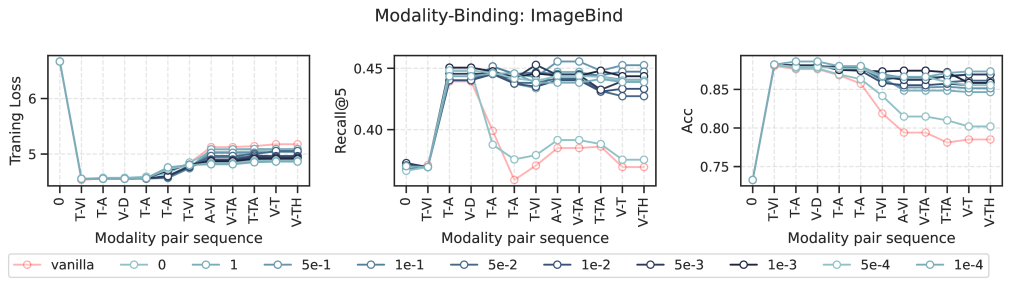
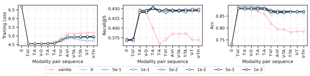
Figure 4: Detailed training loss (left), recall@5 (middle), and accuracy (right) results on the data at the first step. The top figure indicates the results about different $\lambda_{\min}$, while the bottom is for different weight decays, with ImageBind as the backbone. The red line indicates the performance of the vanilla method in CMCL.

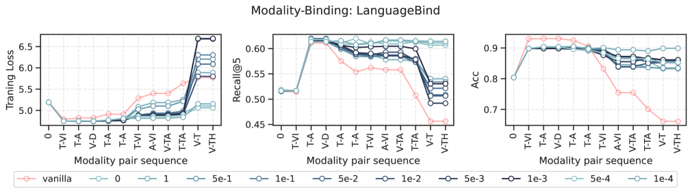
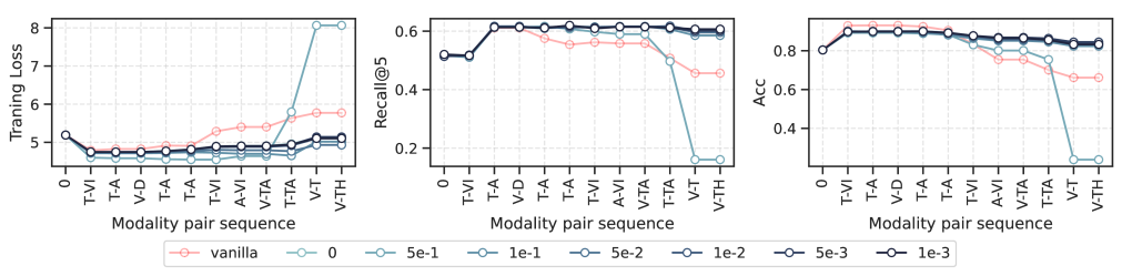
Figure 5: Detailed training loss (left), recall@5 (middle), and accuracy (right) results on the data at the first step. The top figure indicates the results about different $\lambda_{\min}$, while the bottom is for different weight decays, with LanguageBind as the backbone. The red line indicates the performance of the vanilla method in CMCL.

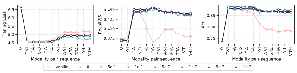
Figure 6: Detailed training loss (left), recall@5 (middle), and accuracy (right) results on the data at the first step. The top figure indicates the results about different $\lambda_{\min}$, while the bottom is for different weight decays, with UniBind as the backbone. The red line indicates the performance of the vanilla method in CMCL.

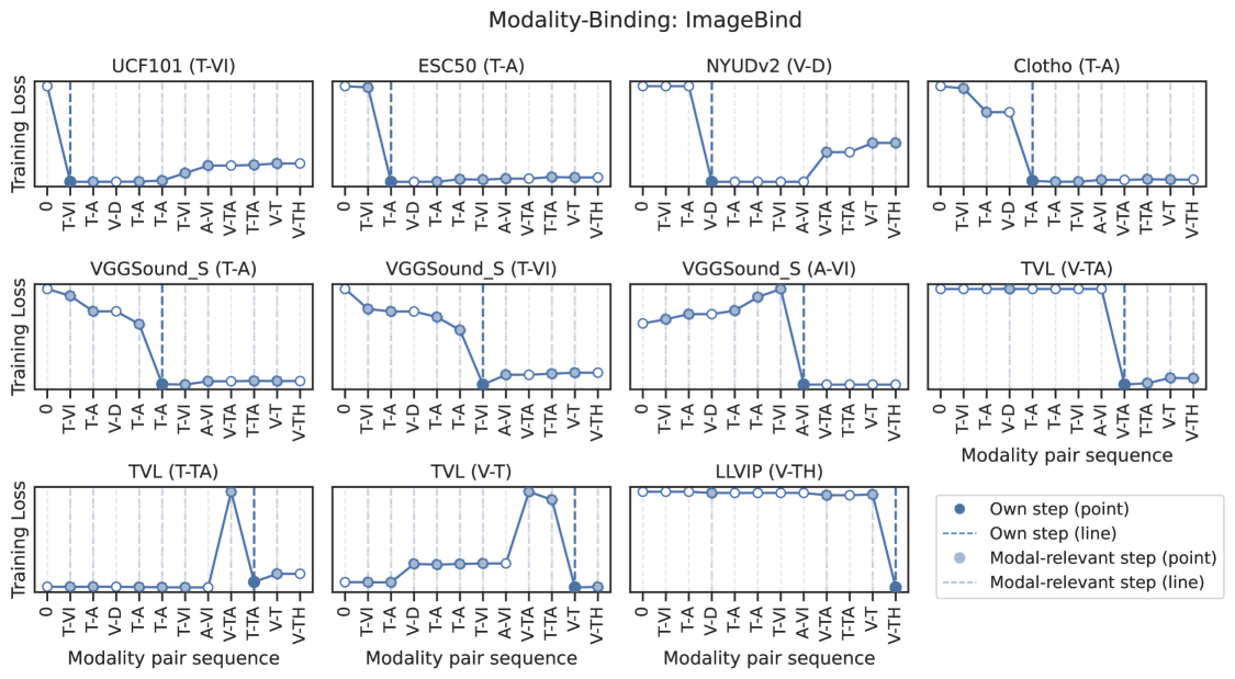
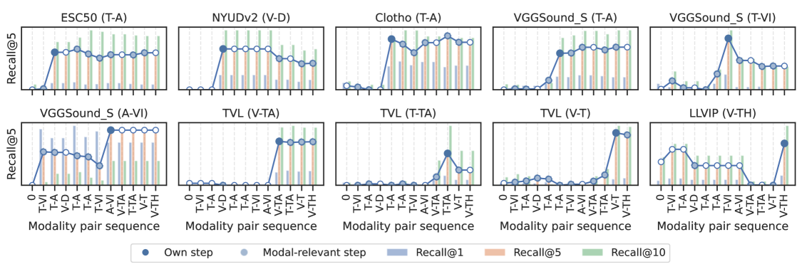
Figure 7: Detailed experimental results of the training loss (the top three rows) and recall (the last two rows) over a sequence of modality pair data, with ImageBind as the modality-binding backbone. Notably, the y-values are normalized for better visualization.

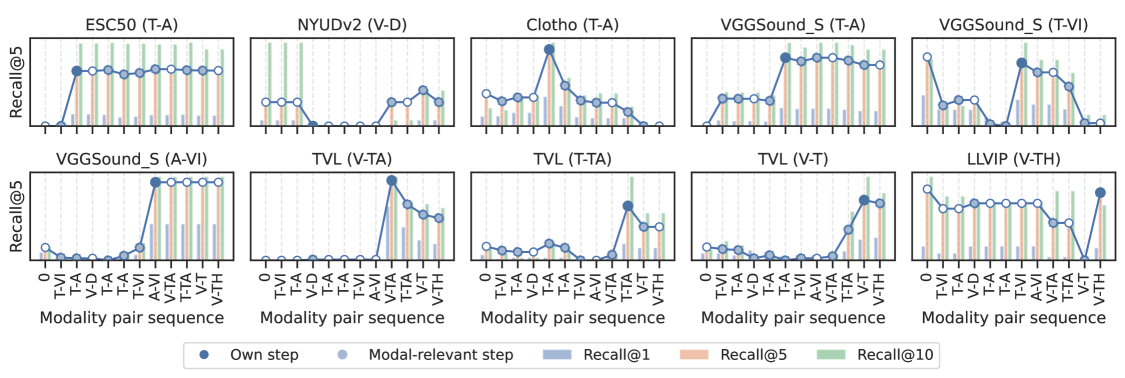
Figure 8: Detailed experimental results of the training loss (the top three rows) and recall (the last two rows) over a sequence of modality pair data, with LanguageBind as the modality-binding backbone. Notably, the y-values are normalized for better visualization.

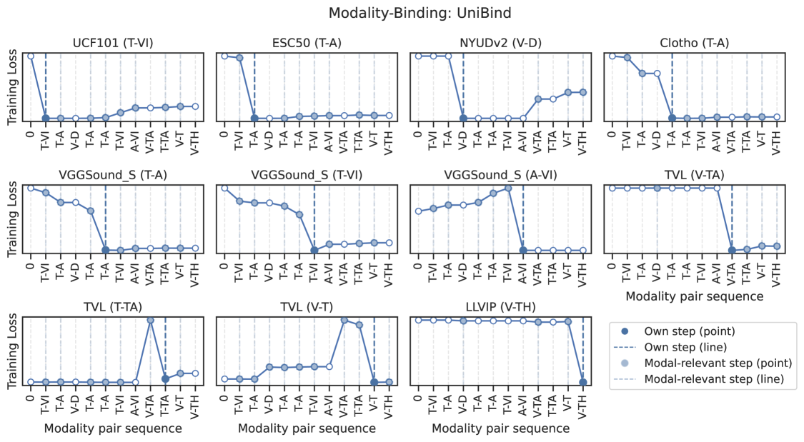
Figure 9: Detailed experimental results of the training loss (the top three rows) and recall (the last two rows) over a sequence of modality pair data, with UniBind as the modality-binding backbone. Notably, the y-values are normalized for better visualization.

Appendix G Impact Statement

This research aims to contribute positively to the machine learning and multimodal learning fields by advancing continual multimodal contrastive learning, which enables models to dynamically integrate and retain knowledge from diverse multimodal data sources over time. Although we believe our work is unlikely to have direct negative societal impacts, we acknowledge the importance of considering potential misuse scenarios, such as the exploitation of continuously adapting systems in unethical surveillance or misinformation campaigns. The broader implication of our study is that it elevates multimodal models with the capability to seamlessly adapt to evolving multimodal environments with minimal retraining, which makes them particularly suitable for real-time applications in adaptive human-computer interaction and autonomous systems. Such advancements could lead to more versatile, resilient, and context-aware AI applications across various real-world domains.

Appendix H Reproducibility

We provide comprehensive implementation details, including illustrative algorithm flows and core pseudo-code. Additionally, source codes will be publicly released.

Appendix I Limitations

This paper fills in the blank of continual multimodal contrastive learning in the development of both multimodal learning and continual learning research. Specifically, this paper introduces a method that projects the gradient onto specialized subspaces, where the incorporation of new data does not interfere with previously acquired knowledge. Although our work is supported by systematic theoretical analyses and empirical studies, it does not yet examine the generalization errors [92] of the proposed method in downstream tasks. We regard addressing the limitation as our future direction.

References

- [1] Tadas Baltrušaitis, Chaitanya Ahuja, and Louis-Philippe Morency. Multimodal machine learning: A survey and taxonomy. IEEE Transactions on Pattern Analysis and Machine Intelligence, 2018.
- [2] Dianzhi Yu, Xinni Zhang, Yankai Chen, Aiwei Liu, Yifei Zhang, Philip S Yu, and Irwin King. Recent advances of multimodal continual learning: A comprehensive survey. arXiv preprint arXiv:2410.05352, 2024.
- [3] Peng Xu, Xiatian Zhu, and David A Clifton. Multimodal learning with transformers: A survey. IEEE Transactions on Pattern Analysis and Machine Intelligence, 45(10):12113–12132, 2023.
- [4] Xiaohao Liu, Xiaobo Xia, Zhuo Huang, and Tat-Seng Chua. Towards modality generalization: A benchmark and prospective analysis. arXiv preprint arXiv:2412.18277, 2024.
- [5] Run Luo, Haonan Zhang, Longze Chen, Ting-En Lin, Xiong Liu, Yuchuan Wu, Min Yang, Minzheng Wang, Pengpeng Zeng, Lianli Gao, et al. Mmevol: Empowering multimodal large language models with evol-instruct. arXiv preprint arXiv:2409.05840, 2024.
- [6] Run Luo, Yunshui Li, Longze Chen, Wanwei He, Ting-En Lin, Ziqiang Liu, Lei Zhang, Zikai Song, Xiaobo Xia, Tongliang Liu, et al. Deem: Diffusion models serve as the eyes of large language models for image perception. arXiv preprint arXiv:2405.15232, 2024.
- [7] Ting Chen, Simon Kornblith, Mohammad Norouzi, and Geoffrey Hinton. A simple framework for contrastive learning of visual representations. In ICML, pages 1597–1607, 2020.
- [8] Kaiming He, Haoqi Fan, Yuxin Wu, Saining Xie, and Ross Girshick. Momentum contrast for unsupervised visual representation learning. In CVPR, pages 9729–9738, 2020.
- [9] Xinlei Chen, Haoqi Fan, Ross Girshick, and Kaiming He. Improved baselines with momentum contrastive learning. arXiv preprint arXiv:2003.04297, 2020.
- [10] Han Zhang, Jing Yu Koh, Jason Baldridge, Honglak Lee, and Yinfei Yang. Cross-modal contrastive learning for text-to-image generation. In CVPR, pages 833–842, 2021.
- [11] Alec Radford, Jong Wook Kim, Chris Hallacy, Aditya Ramesh, Gabriel Goh, Sandhini Agarwal, Girish Sastry, Amanda Askell, Pamela Mishkin, Jack Clark, et al. Learning transferable visual models from natural language supervision. In ICML, pages 8748–8763, 2021.
- [12] Rohit Girdhar, Alaaeldin El-Nouby, Zhuang Liu, Mannat Singh, Kalyan Vasudev Alwala, Armand Joulin, and Ishan Misra. Imagebind: One embedding space to bind them all. In CVPR, pages 15180–15190, 2023.
- [13] Shaohan Huang, Li Dong, Wenhui Wang, Yaru Hao, Saksham Singhal, Shuming Ma, Tengchao Lv, Lei Cui, Owais Khan Mohammed, Barun Patra, et al. Language is not all you need: Aligning perception with language models. In NeurIPS, pages 72096–72109, 2023.
- [14] Yuanhuiyi Lyu, Xu Zheng, Jiazhou Zhou, and Lin Wang. Unibind: Llm-augmented unified and balanced representation space to bind them all. In CVPR, pages 26752–26762, 2024.
- [15] Zehan Wang, Ziang Zhang, Xize Cheng, Rongjie Huang, Luping Liu, Zhenhui Ye, Haifeng Huang, Yang Zhao, Tao Jin, Peng Gao, et al. Freebind: Free lunch in unified multimodal space via knowledge fusion. arXiv preprint arXiv:2405.04883, 2024.
- [16] Bin Zhu, Bin Lin, Munan Ning, Yang Yan, Jiaxi Cui, HongFa Wang, Yatian Pang, Wenhao Jiang, Junwu Zhang, Zongwei Li, et al. Languagebind: Extending video-language pretraining to n-modality by language-based semantic alignment. arXiv preprint arXiv:2310.01852, 2023.
- [17] Shipeng Wang, Xiaorong Li, Jian Sun, and Zongben Xu. Training networks in null space of feature covariance for continual learning. In CVPR, pages 184–193, 2021.
- [18] Hyuntak Cha, Jaeho Lee, and Jinwoo Shin. Co2l: Contrastive continual learning. In ICCV, pages 9516–9525, 2021.
- [19] Yichen Wen, Zhiquan Tan, Kaipeng Zheng, Chuanlong Xie, and Weiran Huang. Provable contrastive continual learning. In ICML, pages 52819–52838, 2024.
- [20] Shipeng Wang, Xiaorong Li, Jian Sun, and Zongben Xu. Training networks in null space of feature covariance with self-supervision for incremental learning. IEEE Transactions on Pattern Analysis and Machine Intelligence, 2024.
- [21] Shengqiong Wu, Hao Fei, Leigang Qu, Wei Ji, and Tat-Seng Chua. Next-gpt: Any-to-any multimodal llm. In ICML, 2024.
- [22] Jiaming Han, Renrui Zhang, Wenqi Shao, Peng Gao, Peng Xu, Han Xiao, Kaipeng Zhang, Chris Liu, Song Wen, Ziyu Guo, et al. Imagebind-llm: Multi-modality instruction tuning. arXiv preprint arXiv:2309.03905, 2023.
- [23] Lei Zhang, Yunshui Li, Jiaming Li, Xiaobo Xia, Jiaxi Yang, Run Luo, Minzheng Wang, Longze Chen, Junhao Liu, and Min Yang. Hierarchical context pruning: Optimizing real-world code completion with repository-level pretrained code llms. arXiv preprint arXiv:2406.18294, 2024.
- [24] Benjamin Elizalde, Soham Deshmukh, Mahmoud Al Ismail, and Huaming Wang. Clap learning audio concepts from natural language supervision. In ICASSP, pages 1–5, 2023.
- [25] Hu Xu, Gargi Ghosh, Po-Yao Huang, Dmytro Okhonko, Armen Aghajanyan, Florian Metze, Luke Zettlemoyer, and Christoph Feichtenhofer. Videoclip: Contrastive pre-training for zero-shot video-text understanding. arXiv preprint arXiv:2109.14084, 2021.
- [26] Chao Jia, Yinfei Yang, Ye Xia, Yi-Ting Chen, Zarana Parekh, Hieu Pham, Quoc Le, Yun-Hsuan Sung, Zhen Li, and Tom Duerig. Scaling up visual and vision-language representation learning with noisy text supervision. In ICML, pages 4904–4916, 2021.
- [27] Shuo Chen, Chen Gong, Jun Li, Jian Yang, Gang Niu, and Masashi Sugiyama. Learning contrastive embedding in low-dimensional space. In NeurIPS, pages 6345–6357, 2022.
- [28] Khurram Soomro, Amir Roshan Zamir, and Mubarak Shah. Ucf101: A dataset of 101 human actions classes from videos in the wild. arXiv preprint arXiv:1212.0402, 2012.
- [29] Karol J Piczak. Esc: Dataset for environmental sound classification. In ACM MM, pages 1015–1018, 2015.
- [30] Pushmeet Kohli Nathan Silberman, Derek Hoiem and Rob Fergus. Indoor segmentation and support inference from rgbd images. In ECCV, 2012.
- [31] Honglie Chen, Weidi Xie, Andrea Vedaldi, and Andrew Zisserman. Vggsound: A large-scale audio-visual dataset. In ICASSP, pages 721–725, 2020.
- [32] Konstantinos Drossos, Samuel Lipping, and Tuomas Virtanen. Clotho: An audio captioning dataset. In ICASSP, pages 736–740, 2020.
- [33] Letian Fu, Gaurav Datta, Huang Huang, William Chung-Ho Panitch, Jaimyn Drake, Joseph Ortiz, Mustafa Mukadam, Mike Lambeta, Roberto Calandra, and Ken Goldberg. A touch, vision, and language dataset for multimodal alignment. arXiv preprint arXiv:2402.13232, 2024.
- [34] Xinyu Jia, Chuang Zhu, Minzhen Li, Wenqi Tang, and Wenli Zhou. Llvip: A visible-infrared paired dataset for low-light vision. In ICCV, pages 3496–3504, 2021.
- [35] Adam Paszke, Sam Gross, Francisco Massa, Adam Lerer, James Bradbury, Gregory Chanan, Trevor Killeen, Zeming Lin, Natalia Gimelshein, Luca Antiga, et al. Pytorch: An imperative style, high-performance deep learning library. In NeurIPS, 2019.
- [36] Ilya Loshchilov and Frank Hutter. Decoupled weight decay regularization. In ICLR, 2019.
- [37] David Lopez-Paz and Marc’Aurelio Ranzato. Gradient episodic memory for continual learning. In NeurIPS, 2017.
- [38] Pietro Buzzega, Matteo Boschini, Angelo Porrello, Davide Abati, and Simone Calderara. Dark experience for general continual learning: a strong, simple baseline. In NeurIPS, pages 15920–15930, 2020.
- [39] James Kirkpatrick, Razvan Pascanu, Neil Rabinowitz, Joel Veness, Guillaume Desjardins, Andrei A Rusu, Kieran Milan, John Quan, Tiago Ramalho, Agnieszka Grabska-Barwinska, et al. Overcoming catastrophic forgetting in neural networks. Proceedings of the National Academy of Sciences, 114(13):3521–3526, 2017.
- [40] Ang Bian, Wei Li, Hangjie Yuan, Mang Wang, Zixiang Zhao, Aojun Lu, Pengliang Ji, Tao Feng, et al. Make continual learning stronger via c-flat. In NeurIPS, pages 7608–7630, 2024.
- [41] Wofk, Diana and Ma, Fangchang and Yang, Tien-Ju and Karaman, Sertac and Sze, Vivienne. FastDepth: Fast Monocular Depth Estimation on Embedded Systems. In ICRA, 2019.
- [42] Justin Kerr, Huang Huang, Albert Wilcox, Ryan Hoque, Jeffrey Ichnowski, Roberto Calandra, and Ken Goldberg. Self-supervised visuo-tactile pretraining to locate and follow garment features. arXiv preprint arXiv:2209.13042, 2022.
- [43] Josh Achiam, Steven Adler, Sandhini Agarwal, Lama Ahmad, Ilge Akkaya, Florencia Leoni Aleman, Diogo Almeida, Janko Altenschmidt, Sam Altman, Shyamal Anadkat, et al. Gpt-4 technical report. arXiv preprint arXiv:2303.08774, 2023.
- [44] Jort F Gemmeke, Daniel PW Ellis, Dylan Freedman, Aren Jansen, Wade Lawrence, R Channing Moore, Manoj Plakal, and Marvin Ritter. Audio set: An ontology and human-labeled dataset for audio events. In ICASSP, pages 776–780, 2017.
- [45] Shuran Song, Samuel P Lichtenberg, and Jianxiong Xiao. Sun rgb-d: A rgb-d scene understanding benchmark suite. In CVPR, pages 567–576, 2015.
- [46] Kristen Grauman, Andrew Westbury, Eugene Byrne, Zachary Chavis, Antonino Furnari, Rohit Girdhar, Jackson Hamburger, Hao Jiang, Miao Liu, Xingyu Liu, et al. Ego4d: Around the world in 3,000 hours of egocentric video. In CVPR, pages 18995–19012, 2022.
- [47] Sami Abu-El-Haija, Nisarg Kothari, Joonseok Lee, Paul Natsev, George Toderici, Balakrishnan Varadarajan, and Sudheendra Vijayanarasimhan. Youtube-8m: A large-scale video classification benchmark. arXiv preprint arXiv:1609.08675, 2016.
- [48] Jun Xu, Tao Mei, Ting Yao, and Yong Rui. Msr-vtt: A large video description dataset for bridging video and language. In CVPR, pages 5288–5296, 2016.
- [49] Tsung-Yi Lin, Michael Maire, Serge Belongie, James Hays, Pietro Perona, Deva Ramanan, Piotr Dollár, and C Lawrence Zitnick. Microsoft coco: Common objects in context. In ECCV, pages 740–755, 2014.
- [50] Chunhui Gu, Chen Sun, David A Ross, Carl Vondrick, Caroline Pantofaru, Yeqing Li, Sudheendra Vijayanarasimhan, George Toderici, Susanna Ricco, Rahul Sukthankar, et al. Ava: A video dataset of spatio-temporally localized atomic visual actions. In CVPR, pages 6047–6056, 2018.
- [51] Hildegard Kuehne, Hueihan Jhuang, Estíbaliz Garrote, Tomaso Poggio, and Thomas Serre. Hmdb: a large video database for human motion recognition. In ICCV, pages 2556–2563, 2011.
- [52] Jia Deng, Wei Dong, Richard Socher, Li-Jia Li, Kai Li, and Li Fei-Fei. Imagenet: A large-scale hierarchical image database. In CVPR, pages 248–255, 2009.
- [53] Hugo Touvron, Thibaut Lavril, Gautier Izacard, Xavier Martinet, Marie-Anne Lachaux, Timothée Lacroix, Baptiste Rozière, Naman Goyal, Eric Hambro, Faisal Azhar, et al. Llama: Open and efficient foundation language models. arXiv preprint arXiv:2302.13971, 2023.
- [54] Junnan Li, Dongxu Li, Silvio Savarese, and Steven Hoi. Blip-2: Bootstrapping language-image pre-training with frozen image encoders and large language models. In ICML, pages 19730–19742, 2023.
- [55] Renrui Zhang, Jiaming Han, Chris Liu, Peng Gao, Aojun Zhou, Xiangfei Hu, Shilin Yan, Pan Lu, Hongsheng Li, and Yu Qiao. Llama-adapter: Efficient fine-tuning of language models with zero-init attention. arXiv preprint arXiv:2303.16199, 2023.
- [56] Roger Penrose. A generalized inverse for matrices. In Mathematical proceedings of the Cambridge philosophical society, volume 51, pages 406–413, 1955.
- [57] JK Baksalary and R Kala. The matrix equation ax- yb= c. Linear Algebra and its Applications, 25:41–43, 1979.
- [58] Mohammadreza Zolfaghari, Yi Zhu, Peter Gehler, and Thomas Brox. Crossclr: Cross-modal contrastive learning for multi-modal video representations. In ICCV, pages 1450–1459, 2021.
- [59] Yiwei Zhou, Xiaobo Xia, Zhiwei Lin, Bo Han, and Tongliang Liu. Few-shot adversarial prompt learning on vision-language models. In NeurIPS, pages 3122–3156, 2024.
- [60] Shikun Li, Xiaobo Xia, Shiming Ge, and Tongliang Liu. Selective-supervised contrastive learning with noisy labels. In CVPR, pages 316–325, 2022.
- [61] Andrey Guzhov, Federico Raue, Jörn Hees, and Andreas Dengel. Audioclip: Extending clip to image, text and audio. In ICASSP, pages 976–980, 2022.
- [62] Ho-Hsiang Wu, Prem Seetharaman, Kundan Kumar, and Juan Pablo Bello. Wav2clip: Learning robust audio representations from clip. In ICASSP, pages 4563–4567, 2022.
- [63] Ziyu Guo, Renrui Zhang, Xiangyang Zhu, Yiwen Tang, Xianzheng Ma, Jiaming Han, Kexin Chen, Peng Gao, Xianzhi Li, Hongsheng Li, et al. Point-bind & point-llm: Aligning point cloud with multi-modality for 3d understanding, generation, and instruction following. arXiv preprint arXiv:2309.00615, 2023.
- [64] Zehan Wang, Ziang Zhang, Hang Zhang, Luping Liu, Rongjie Huang, Xize Cheng, Hengshuang Zhao, and Zhou Zhao. Omnibind: Large-scale omni multimodal representation via binding spaces. arXiv preprint arXiv:2407.11895, 2024.
- [65] Oriol Barbany, Michael Huang, Xinliang Zhu, and Arnab Dhua. Leveraging large language models for multimodal search. In CVPR, pages 1201–1210, 2024.
- [66] Sheng-Chieh Lin, Chankyu Lee, Mohammad Shoeybi, Jimmy Lin, Bryan Catanzaro, and Wei Ping. Universal multimodal retrieval with multimodal llms. In ICLR, 2025.
- [67] Felix Kreuk, Gabriel Synnaeve, Adam Polyak, Uriel Singer, Alexandre Défossez, Jade Copet, Devi Parikh, Yaniv Taigman, and Yossi Adi. Audiogen: Textually guided audio generation. arXiv preprint arXiv:2209.15352, 2022.
- [68] Jade Copet, Felix Kreuk, Itai Gat, Tal Remez, David Kant, Gabriel Synnaeve, Yossi Adi, and Alexandre Défossez. Simple and controllable music generation. In NeurIPS, pages 47704–47720, 2023.
- [69] Robin Rombach, Andreas Blattmann, Dominik Lorenz, Patrick Esser, and Björn Ommer. High-resolution image synthesis with latent diffusion models. In CVPR, pages 10684–10695, 2022.
- [70] Zijing Liang, Yanjie Xu, Yifan Hong, Penghui Shang, Qi Wang, Qiang Fu, and Ke Liu. A survey of multimodel large language models. In CAICE, pages 405–409, 2024.
- [71] Runpei Dong, Chunrui Han, Yuang Peng, Zekun Qi, Zheng Ge, Jinrong Yang, Liang Zhao, Jianjian Sun, Hongyu Zhou, Haoran Wei, et al. Dreamllm: Synergistic multimodal comprehension and creation. In ICLR, 2024.
- [72] Yiping Wang, Yifang Chen, Wendan Yan, Alex Fang, Wenjing Zhou, Kevin G Jamieson, and Simon S Du. Cliploss and norm-based data selection methods for multimodal contrastive learning. In NeurIPS, pages 15028–15069, 2024.
- [73] Simon Schrodi, David T Hoffmann, Max Argus, Volker Fischer, and Thomas Brox. Two effects, one trigger: on the modality gap, object bias, and information imbalance in contrastive vision-language representation learning. arXiv preprint arXiv:2404.07983, 2024.
- [74] Zhuo Huang, Gang Niu, Bo Han, Masashi Sugiyama, and Tongliang Liu. Towards out-of-modal generalization without instance-level modal correspondence. In ICLR, 2025.
- [75] Sebastian Thrun and Tom M Mitchell. Lifelong robot learning. Robotics and Autonomous Systems, 15(1-2):25–46, 1995.
- [76] Liyuan Wang, Xingxing Zhang, Hang Su, and Jun Zhu. A comprehensive survey of continual learning: Theory, method and application. IEEE Transactions on Pattern Analysis and Machine Intelligence, 2024.
- [77] Ameya Prabhu, Philip HS Torr, and Puneet K Dokania. Gdumb: A simple approach that questions our progress in continual learning. In ECCV, pages 524–540, 2020.
- [78] Matthew Riemer, Ignacio Cases, Robert Ajemian, Miao Liu, Irina Rish, Yuhai Tu, and Gerald Tesauro. Learning to learn without forgetting by maximizing transfer and minimizing interference. arXiv preprint arXiv:1810.11910, 2018.
- [79] Zhizhong Li and Derek Hoiem. Learning without forgetting. IEEE Transactions on Pattern Analysis and Machine Intelligence, 40(12):2935–2947, 2017.
- [80] Xialei Liu, Marc Masana, Luis Herranz, Joost Van de Weijer, Antonio M Lopez, and Andrew D Bagdanov. Rotate your networks: Better weight consolidation and less catastrophic forgetting. In ICPR, pages 2262–2268, 2018.
- [81] Kibok Lee, Kimin Lee, Jinwoo Shin, and Honglak Lee. Overcoming catastrophic forgetting with unlabeled data in the wild. In ICCV, pages 312–321, 2019.
- [82] Itay Evron, Edward Moroshko, Rachel Ward, Nathan Srebro, and Daniel Soudry. How catastrophic can catastrophic forgetting be in linear regression? In COLT, pages 4028–4079, 2022.
- [83] Xuyang Zhao, Huiyuan Wang, Weiran Huang, and Wei Lin. A statistical theory of regularization-based continual learning. In ICML, 2024.
- [84] Jaehong Yoon, Saehoon Kim, Eunho Yang, and Sung Ju Hwang. Scalable and order-robust continual learning with additive parameter decomposition. In ICLR, 2020.
- [85] Ching-Yi Hung, Cheng-Hao Tu, Cheng-En Wu, Chien-Hung Chen, Yi-Ming Chan, and Chu-Song Chen. Compacting, picking and growing for unforgetting continual learning. In NeurIPS, 2019.
- [86] Jaehong Yoon, Eunho Yang, Jeongtae Lee, and Sung Ju Hwang. Lifelong learning with dynamically expandable networks. In ICLR, 2018.
- [87] Gido M Van de Ven, Tinne Tuytelaars, and Andreas S Tolias. Three types of incremental learning. Nature Machine Intelligence, 4(12):1185–1197, 2022.
- [88] Marc Masana, Xialei Liu, Bartłomiej Twardowski, Mikel Menta, Andrew D Bagdanov, and Joost Van De Weijer. Class-incremental learning: survey and performance evaluation on image classification. IEEE Transactions on Pattern Analysis and Machine Intelligence, 2022.
- [89] Zifeng Wang, Zizhao Zhang, Sayna Ebrahimi, Ruoxi Sun, Han Zhang, Chen-Yu Lee, Xiaoqi Ren, Guolong Su, Vincent Perot, Jennifer Dy, et al. Dualprompt: Complementary prompting for rehearsal-free continual learning. In ECCV, pages 631–648, 2022.
- [90] Zi Qian, Xin Wang, Xuguang Duan, Pengda Qin, Yuhong Li, and Wenwu Zhu. Decouple before interact: Multi-modal prompt learning for continual visual question answering. In ICCV, pages 2953–2962, 2023.
- [91] Yabin Wang, Zhiwu Huang, and Xiaopeng Hong. S-prompts learning with pre-trained transformers: An occam’s razor for domain incremental learning. In NeurIPS, pages 5682–5695, 2022.
- [92] Qi Zhang, Yifei Wang, and Yisen Wang. On the generalization of multi-modal contrastive learning. In ICML, pages 41677–41693, 2023.