Real Eigenvalues of Asymmetric Wishart Matrices:
Expected Number, Global Density and Integrable Structure

Abstract

We investigate the real eigenvalues of asymmetric Wishart matrices of size $N$, indexed by the rectangular parameter $\nu\in\mathbb{N}$ and the non-Hermiticity parameter $\tau\in[0,1]$. The rectangular parameter $\nu$ is either fixed or proportional to $N$. The non-Hermiticity parameter $\tau$ is either fixed or $\tau=1-O(1/N)$, corresponding to the strongly and weakly non-Hermitian regimes, respectively.

We establish a decomposition structure for the finite-$N$ correlation kernel of the real eigenvalues, which form Pfaffian point processes. Taking the symmetric limit $\tau=1$, where the model reduces to the Laguerre orthogonal ensemble, this decomposition structure reduces to the known rank-one perturbation structure established by Adler, Forrester, Nagao, and van Moerbeke, as well as by Widom. Using the decomposition structure, we show that the expected number of real eigenvalues is proportional to $\sqrt{N}$ in the strongly non-Hermitian regime and to $N$ in the weakly non-Hermitian regime, providing explicit leading coefficients in both cases. Furthermore, we derive the limiting real eigenvalue densities, which recovers the Marchenko-Pastur distribution in the symmetric limit.

1 Introduction and main results

For given non-negative integers $N$ and $\nu$, let $\mathrm{P}$ and $\mathrm{Q}$ be $N\times(N+\nu)$ random matrices with independent real Gaussian entries, each having mean 0 and variance $1/(2N)$. The matrices $\mathrm{P}$ and $\mathrm{Q}$ are independent and are referred to as rectangular Ginibre matrices [22]. By definition, the asymmetric Wishart matrix $X$ is given by

$$X:=X_{+}X_{-}^{\mathsf{T}},\qquad X_{\pm}=\sqrt{1+\tau}\,\mathrm{P}\pm\sqrt{1-\tau}\,\mathrm{Q},$$ (1.1)

where $\tau\in[0,1]$ and $A^{\mathsf{T}}$ denotes the transposition of a matrix $A$. Here, the rectangular parameter $\nu\equiv\nu_{N}$ and the non-Hermiticity parameter $\tau\equiv\tau_{N}$ possibly depend on $N$. The model $X$ appears in the literature also under the name of sample cross-covariance matrix or chiral elliptic Ginibre ensemble, and finds applications in various areas such as quantum chromodynamics and ecosystem stability; see e.g. [19, 61, 14, 62] and references therein. Note in particular that the parameter $\tau\in[0,1]$ quantifies the asymmetry of the model. In the extremal, symmetric case when $\tau=1$, the matrix model $X$ becomes the classical Wishart matrix (the Laguerre orthogonal ensemble) [39, Chapter 3].

Beyond the matrix with real elements, the complex and quaternionic counterparts of non-Hermitian Wishart matrices have also been extensively studied in the literature; see e.g. [65, 27, 9, 4, 5, 6, 15, 11, 29, 56] and references therein. A remarkable property of the eigenvalues in the complex and quaternionic cases is their interpretation as one-component Coulomb gas ensembles [39, 67, 22]. In contrast, such a one-component realisation is no longer valid for matrices with real elements. The key distinction lies in the fact that, in the real case, there is a non-trivial probability of having purely real eigenvalues; see Figure 1.

In this paper, we investigate the real eigenvalues of asymmetric Wishart matrices. The main contributions of this work are summarised as follows:

• Expected number of real eigenvalues (Theorem 1.1);

• Macroscopic density of real eigenvalues (Theorem 1.2);

• Decomposition structure of the correlation kernel (Theorem 2.1).

Analogous results in the context of the elliptic Ginibre matrices were established in [36, 46, 24, 37].

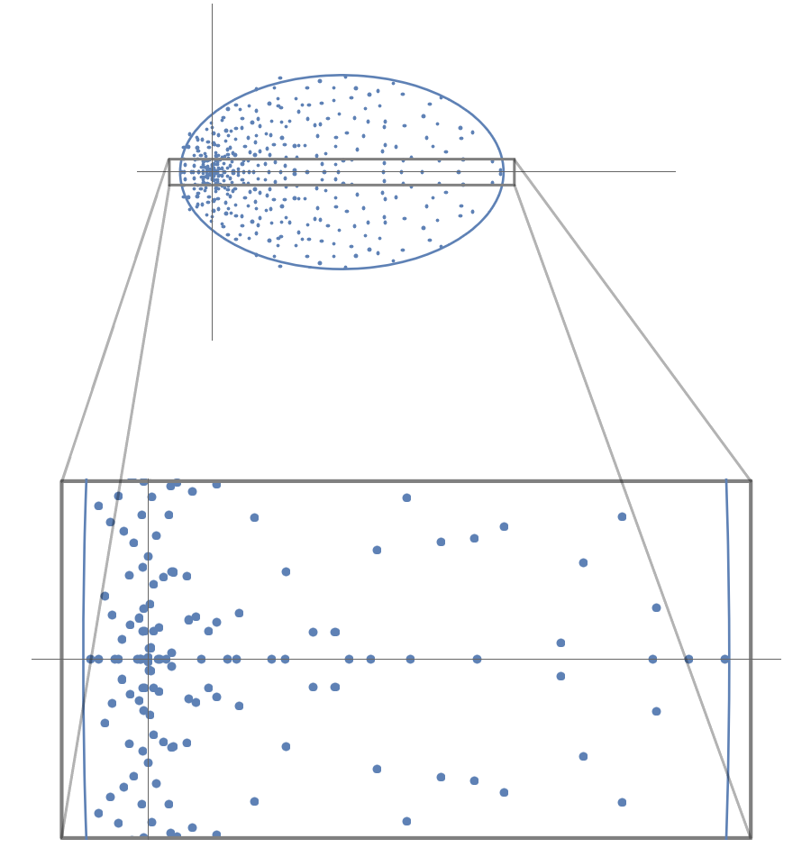
(a) $\nu=0$

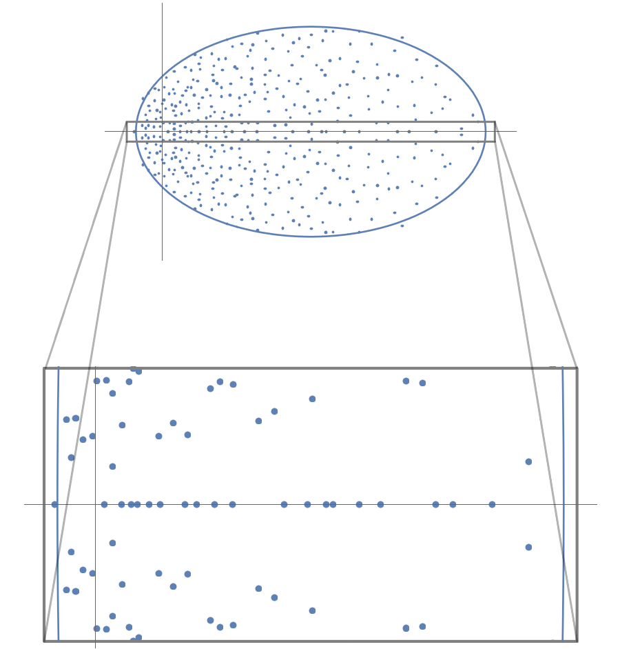
(b) $\nu=N$

Figure 1: The plots show the eigenvalues of asymmetric Wishart matrices with $N=400$ and $\tau=1/2$. In the zoomed-in images, the presence of purely real eigenvalues is clearly visible. Furthermore, in the case of $\nu=0$, there is an accumulation of eigenvalues near the origin, reflecting the divergent density.

In the study of asymmetric Wishart matrices, various interesting regimes emerge, depending on the scaling properties of the parameters.

• Strongly non-Hermitian regime. This is the case where $\tau$ stays away from the extremal, symmetric case $\tau=1$. In particular, we usually consider the case where $\tau\in[0,1)$ is fixed.

• Weakly non-Hermitian regime. This is the case when $\tau\uparrow 1$ with a proper speed. This regime, first pioneered in [50, 51, 52] for the elliptic Ginibre matrices, allows one to observe a non-trivial transition to Hermitian matrices. In particular, we mainly consider the regime $1-\tau=O(N^{-1})$.

• Singular density regime. This is the case where $\nu=o(N)$. In this case, for general $\tau\in[0,1)$, the origin is contained in the limiting spectrum with divergent density; cf. Figure 1 (A).

• Regular density regime. This is the case where $\nu=\varrho N$ with a positive $\varrho>0$. Whether the origin is contained in the limiting spectrum is determined by the sign of $\tau\sqrt{1+\varrho}-1$; see (1.18) and (1.20). If the sign is positive, the origin is included in the spectrum; however, the density at the origin remains bounded. See Figure 1 (B).

Following the notations in the previous literature, we use the parametrisation

$$\tau=1-\frac{\alpha^{2}}{2N},\qquad\alpha>0$$ (1.2)

for the weakly non-Hermitian regime. (See also a recent work [10] where various mesoscopic regimes were explored.) We also note that when discussing macroscopic properties, it is often unnecessary to distinguish between the two cases of rectangular parameters. By combining these cases, one can assume that

$$\lim_{N\to\infty}\frac{\nu}{N}=\varrho\in[0,\infty).$$ (1.3)

In the following, we focus on the case where $N$ is an even integer, as this choice simplifies the overall presentation and analysis. While the case of odd $N$ is also tractable, it requires additional computations. For instance, the odd $N$ case was addressed in [70, 43] for the real Ginibre matrix.

Let $\mathcal{N}\equiv\mathcal{N}_{\tau,\nu}$ denote the number of real eigenvalues. We denote by $\mathbf{R}_{N,k}$ the $k$-point correlation function of real eigenvalues; see [22, Chapter 7]. In particular, the $1$-point function $\mathbf{R}_{N}\equiv\mathbf{R}_{N,1}$ can be characterised by

$$\mathbb{E}\Big{[}\sum_{j=1}^{\mathcal{N}}f(x_{j})\Big{]}=\int_{\mathbb{R}}f(x)\,\mathbf{R}_{N}(x)\,dx,$$ (1.4)

where $f$ is a test function. For general $k$, the correlation function $\mathbf{R}_{N,k}$ can be written explicitly in terms of a certain Pfaffian; see (2.7) below.

When exploring the real eigenvalues of asymmetric random matrices, a natural object of interest is their number/counting statistics. A fundamental aspect of this is determining the typical number of real eigenvalues. This has been studied in various models, beginning with the seminal work on the real Ginibre matrix [36, 45] and extending to its variants, including the elliptic Ginibre matrix in both the strongly [46] and weakly [24] non-Hermitian regimes, as well as truncated matrices and their products [48, 60, 47], spherical ensembles [36, 44], and products of Ginibre matrices [7, 69, 40]. Furthermore, [72] established that matrices with general i.i.d. elements asymptotically exhibit the same number of real eigenvalues, thereby demonstrating universality. (We also refer the reader to [30, 16, 8, 53, 33, 55] and the references therein for the counting statistics of various two-dimensional point processes.)

In this work, we address these questions for asymmetric Wishart matrices. For this purpose, let

$$E_{N,\tau}^{\nu}:=\mathbb{E}\mathcal{N}=\int_{\mathbb{R}}\mathbf{R}_{N}(x)\,dx$$ (1.5)

be the expected number of real eigenvalues of $X$. Here, the second identity follows from (1.4). We write

$$\xi_{\pm}:=\tau(2+\varrho)\pm(1+\tau^{2})\sqrt{1+\varrho}.$$ (1.6)

Recall that the modified Bessel function $I_{\nu}$ of the first kind is given by

$$I_{\nu}(z):=\sum_{k=0}^{\infty}\frac{(z/2)^{2k+\nu}}{k!\,\Gamma(\nu+k+1)};$$ (1.7)

see e.g. [64, Chapter 10].

Theorem 1.1 (Expected number of real eigenvalues).

Suppose that $\nu=\varrho N$ with $\varrho>0$ fixed, or that $\nu\geq 0$ is fixed.

• (Strongly non-Hermitian regime) Let $\tau\in[0,1)$ be fixed. Then as $N\to\infty,$ we have

  $$E_{N,\tau}^{\nu}=\Big{(}\frac{1}{4\pi}\frac{N}{1-\tau^{2}}\Big{)}^{\frac{1}{2}}c(\tau,\varrho)+o(\sqrt{N}),$$ (1.8)

  where

  $$\begin{split}c(\tau,\varrho):=\int_{\xi_{-}}^{\xi_{+}}(x^{2}+(1-\tau^{2})^{2}\varrho^{2}/4)^{-\frac{1}{4}}\,dx.\end{split}$$ (1.9)

  Here, $\xi_{\pm}$ are given by (1.6). If $\nu\geq 0$ is fixed, then the result holds with $\varrho=0$.

• (Weakly non-Hermitian regime) Let $\tau$ be given by (1.2). Then as $N\to\infty,$ we have

  $$E_{N,\tau}^{\nu}=c(\alpha)\,N+o(N),$$ (1.10)

  where

  $$c(\alpha):=e^{-\alpha^{2}/2}[I_{0}(\tfrac{\alpha^{2}}{2})+I_{1}(\tfrac{\alpha^{2}}{2})].$$ (1.11)

  Here, $I_{\nu}$ is the modified Bessel function (1.7).

See Figure 2 for the numerics on Theorem 1.1.

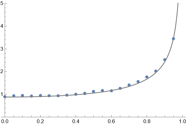
(a) Strong non-Hermiticity

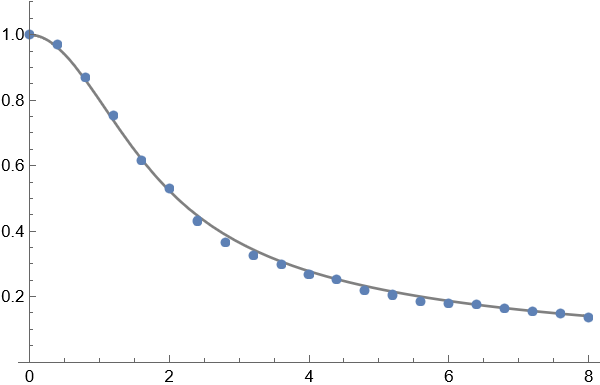
(b) Weak non-Hermiticity

Figure 2: Plot (A) shows $\tau\mapsto E_{N,\tau}^{\nu}/\sqrt{N}$ (blue dots) and its comparison with $c(\tau,\varrho)$ (solid gray line). Plot (B) illustrates $\alpha\mapsto E_{N,\tau}^{\nu}/N$ (blue dots) for $\tau$ given by (1.2), compared to $c(\alpha)$ (solid gray line). Here, we use 20 samples of $X$ with size $N=400$ and $\nu=N$.

Remark 1.1 (Alternative expressions).

The coefficient $c(\tau,\varrho)$ in (1.9) can also be expressed as

$$c(\tau,\varrho)=\sqrt{\frac{2}{\varrho}}(1-\tau^{2})^{-\frac{1}{2}}\bigg{[}{}_{2}F_{1}\Big{(}\frac{1}{4},\frac{1}{2};\frac{3}{2};-\frac{4\xi_{+}^{2}}{\varrho^{2}(1-\tau^{2})^{2}}\Big{)}\xi_{+}-{}_{2}F_{1}\Big{(}\frac{1}{4},\frac{1}{2};\frac{3}{2};-\frac{4\xi_{-}^{2}}{\varrho^{2}(1-\tau^{2})^{2}}\Big{)}\xi_{-}\bigg{]},$$ (1.12)

where ${}_{2}F_{1}$ is the hypergeometric function, which can be defined by the Euler integral formula

$${}_{2}F_{1}(a,b,c,z)=\frac{1}{\Gamma(b)\Gamma(c)\Gamma(c-b)}\int_{0}^{1}\frac{t^{b-1}(1-t)^{c-b-1}}{(1-zt)^{a}}\,dt,\qquad(c>b>0);$$ (1.13)

see e.g. [64, Chapter 15]. On the other hand, by using (1.7), the coefficient $c(\alpha)$ in (1.11) can be written as

$$c(\alpha)=\sum_{k=0}^{\infty}\frac{(2k-1)!!}{2^{k}\,k!\,(k+1)!}(-1)^{k}\alpha^{2k}.$$ (1.14)

Remark 1.2 (Special case $\varrho=0$ and comparison with previous results at strong non-Hermiticity).

By letting $\varrho=0$ in (1.9), one can see that $c(\tau,0)=4$. Therefore, if $\nu$ is fixed, the asymptotic behaviour (1.15) becomes simplified as

$$E_{N,\tau}^{\nu}\Big{|}_{\varrho=0}=\Big{(}\frac{4}{\pi}\frac{N}{1-\tau^{2}}\Big{)}^{\frac{1}{2}}+o(\sqrt{N}).$$ (1.15)

This formula was previously proposed in [66, Chapter 6] using the Dirac picture of the matrix model.

For the special case when $\tau=\nu=0$, the asymmetric Wishart matrix $X$ reduces to the product of two Ginibre matrices. For general fixed $m\in\mathbb{N}$, it was obtained in [69] that the expected number of real eigenvalues of products of $m$ independent Ginibre matrices is asymptotically $(2mN/\pi)^{1/2}$. One can observe that this formula for $m=2$ agrees with (1.15) for $\tau=0$.

Remark 1.3 (Independence of the rectangular parameter at weak non-Hermiticity).

In the strongly non-Hermitian regime, the leading-order coefficient in (1.8) depends on the rectangular parameter $\nu=\varrho N$. In contrast, the leading asymptotic behaviour at weak non-Hermiticity is independent of the order of the rectangular parameter $\nu$. In other words, in (1.10), the coefficient $c(\alpha)$ depends only on $\alpha$ and not on $\varrho$.

Moreover, the function $c(\alpha)$ also arises in the context of the elliptic Ginibre matrices at weak non-Hermiticity; see [24, Theorem 2.1]. These observations suggest a possible universal phenomenon, indicating that the function $c(\alpha)$ might appear in a broader class of random matrix ensembles.

We now present the limiting density of the real eigenvalues. First, recall that in the extremal symmetric case when $\tau=1$, the limiting empirical distribution is given by the celebrated Marchenko-Pastur law [63]

$$\rho_{\textup{MP},\varrho}(x):=\mathbbm{1}_{[\lambda_{-},\lambda_{+}]}(x)\cdot\frac{1}{2\pi}\frac{\sqrt{(\lambda_{+}-x)(x-\lambda_{-})}}{x},\qquad\lambda_{\pm}=(\sqrt{\varrho+1}\pm 1)^{2}.$$ (1.16)

For a fixed $\tau\in[0,1)$, it was shown that the limiting empirical distribution of the total (complex and real) eigenvalues is given by the non-Hermitian extension of the Marchenko-Pastur law (also called shifted elliptic law) [75, 9]

$$d\mu(z):=\frac{1}{1-\tau^{2}}\frac{1}{\sqrt{4|z|^{2}+(1-\tau^{2})^{2}\varrho^{2}}}\cdot\mathbbm{1}_{S_{\varrho}}(z)\,\frac{d^{2}z}{\pi},$$ (1.17)

where

$$S_{\varrho}:=\Big{\{}(x,y)\in\mathbb{R}^{2}:\Big{(}\frac{x-\tau(2+\varrho)}{(1+\tau^{2})\sqrt{1+\varrho}}\Big{)}^{2}+\Big{(}\frac{y}{(1-\tau^{2})\sqrt{1+\varrho}}\Big{)}^{2}\leq 1\Big{\}}.$$ (1.18)

Observe here that for each $\tau\in[0,1)$ the right and left endpoints of $S_{\varrho}$ are given by $\xi_{\pm}$ in (1.6). Furthermore, one can also notice that the endpoints $\lambda_{\pm}$ of the Marchenko-Pastur law (1.16) corresponds to the symmetric limits of $\xi_{\pm}$, i.e. $\lambda_{\pm}:=\lim_{\tau\to 1}\xi_{\pm}.$

However, the limiting distribution (1.17) does not provide direct information about the real eigenvalues. As determined in Theorem 1.1, in the strongly non-Hermitian regime, the typical number of real eigenvalues is of order $O(\sqrt{N})$, which is subdominant compared to the total $N$ eigenvalues. Furthermore, in the weakly non-Hermitian regime, no previous work has demonstrated the macroscopic behaviour of the eigenvalues. In the next result, we address both of these aspects.

Let us write

$$\rho_{N,\tau}^{\nu}(x):=\frac{1}{E_{N,\tau}}\mathbf{R}_{N}(x)$$ (1.19)

for the averaged density of real eigenvalues.

Theorem 1.2 (Limiting density of real eigenvalues).

Suppose that $\nu=\varrho N$ with $\varrho>0$ fixed, or that $\nu\geq 0$ is fixed. Then for any bounded continuous test function $f$, we have the following.

• (Strongly non-Hermitian regime) Let $\tau\in[0,1)$ be fixed. Define

  $$\rho_{\tau,\varrho}^{s}(x):=\mathbbm{1}_{[\xi_{-},\xi_{+}]}(x)\cdot\frac{(x^{2}+(1-\tau^{2})^{2}\varrho^{2}/4)^{-\frac{1}{4}}}{c(\tau,\varrho)},$$ (1.20)

  where $c(\tau,\varrho)$ is given by (1.9). Then we have

  $$\lim_{N\to\infty}\int_{\mathbb{R}}f(x)\rho_{N,\tau}^{\nu}(x)\,dx=\int_{\mathbb{R}}f(x)\rho_{\tau,\varrho}^{s}(x)\,dx.$$ (1.21)

  Furthermore, for any fixed $x\in(\xi_{-},\xi_{+})$, we have the pointwise limit

  $$\lim_{N\to\infty}\rho_{N,\tau}^{\nu}(x)=\rho_{\tau,\varrho}^{s}(x).$$ (1.22)

• (Weakly non-Hermitian regime) Let $\tau$ be given by (1.2). Define

  $$\rho_{\alpha,\varrho}^{w}(x):=\mathbbm{1}_{[\lambda_{-},\lambda_{+}]}(x)\cdot\frac{1}{c(\alpha)}\frac{1}{2\alpha\sqrt{\pi}}\frac{1}{\sqrt{x}}\operatorname{erf}\Big{(}\frac{\alpha}{2}\sqrt{\frac{(\lambda_{+}-x)(x-\lambda_{-})}{x}}\Big{)},$$ (1.23)

  where $\operatorname{erf}(x)=\frac{2}{\sqrt{\pi}}\int_{0}^{x}e^{-t^{2}}\,dt$ is the error function. Then we have

  $$\lim_{N\to\infty}\int_{\mathbb{R}}f(x)\rho_{N,\tau}^{\nu}(x)\,dx=\int_{\mathbb{R}}f(x)\rho_{\alpha,\varrho}^{w}(x)\,dx.$$ (1.24)

  Furthermore, for any fixed $x\in(\lambda_{-},\lambda_{+})$, we have the pointwise limit

  $$\lim_{N\to\infty}\rho_{N,\tau}^{\nu}(x)=\rho_{\alpha,\varrho}^{w}(x).$$ (1.25)

See Figure 3 for the numerics.

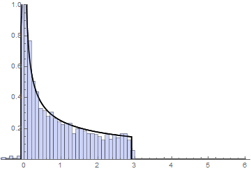
(a) $\nu=0$

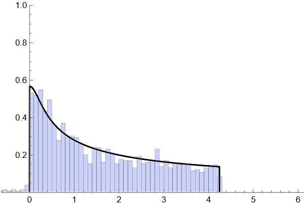
(b) $\nu=N$

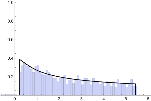
(c) $\nu=2N$

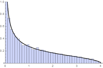
(d) $\nu=0$

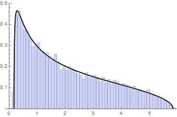
(e) $\nu=N$

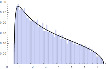
(f) $\nu=2N$

Figure 3: The plots (A)–(C) present histograms of real eigenvalues for 20 samples of $X$ with size $N=2000$, compared to $\rho_{\tau,\varrho}^{s}$, where $\tau=1/\sqrt{2}$. Similarly, the plots (D)–(F) illustrate histograms of real eigenvalues for 20 samples of $X$ with size $N=400$, where $\tau$ is defined by (1.2), compared to $\rho_{\alpha,\varrho}^{w}$, with $\alpha=1$.

Remark 1.4 (Normalisation constants).

By definition (1.9), $c(\tau,\varrho)$ is the normalisation constant that turns $\rho_{\tau,\varrho}^{s}$ into a probability density function. For the weak non-Hermiticity, the mass-one condition of $\rho_{\alpha,\varrho}^{w}$ follows from the identity: for any $\varrho\geq 0$,

$$c(\alpha)=\frac{1}{2\alpha\sqrt{\pi}}\int_{\lambda_{-}}^{\lambda_{+}}\frac{1}{\sqrt{x}}\operatorname{erf}\Big{(}\frac{\alpha}{2}\sqrt{\frac{(\lambda_{+}-x)(x-\lambda_{-})}{x}}\Big{)}\,dx.$$ (1.26)

To show this identity (1.26), one can use the expansion of the error function [64, Eq. (7.6.1)] to write

$$\frac{1}{2\alpha\sqrt{\pi}}\operatorname{erf}\Big{(}\frac{\alpha}{2}\sqrt{\frac{(\lambda_{+}-x)(x-\lambda_{-})}{x}}\Big{)}=\frac{1}{2\pi}\sum_{k=0}^{\infty}\frac{1}{2^{2k}\,k!\,(2k+1)}\Big{(}\frac{(\lambda_{+}-x)(x-\lambda_{-})}{x}\Big{)}^{k+\frac{1}{2}}(-1)^{k}\alpha^{2k}.$$

Then, (1.26) follows from term-by-term integration using the Euler integral formula (1.13) and the identity [64, Eq. (15.4.17)].

Remark 1.5 (Square root relation between complex and real eigenvalue densities at strong non-Hermiticity).

In [73], Tarnowski introduced an interesting relation for general asymmetric random matrices at strong non-Hermiticity: the continuous part of the limiting density of real eigenvalues is proportional to the square root of the limiting density of complex eigenvalues evaluated on the real line. Furthermore, it was observed that this relation holds for certain known real and complex eigenvalue densities, such as those of product matrices. In Theorem 1.2 (i), one can observe that such a square root relation also holds for asymmetric Wishart matrix at strong non-Hermiticity. Namely, up to a multiplicative constant, the density $\rho_{\tau,\varrho}^{s}$ is the square root of that of the equilibrium measure (1.17).

Remark 1.6 (Interpolating properties).

By using the well-known asymptotic behaviours of the error function [64, Eqs. (7.6.1), (7.12.1)] and (1.26), it follows that the function $c(\alpha)$ satisfies

$$c(\alpha)\sim\begin{cases}1&\text{as}\quad\alpha\to 0\,,\\ \frac{2}{\alpha\sqrt{\pi}}&\text{as}\quad\alpha\to\infty\,.\end{cases}$$ (1.27)

These asymptotic behaviours allow us to observe the interpolating properties. In the symmetric limit $\alpha\to 0$, it is obvious that the expected number of real eigenvalues equals the total number of eigenvalues, which is consistent with $Nc(\alpha)\sim N$ as $\alpha\to 0$. Conversely, in the non-Hermitian limit $\alpha\to\infty$, the asymptotic behaviour aligns with the result of Theorem 1.1 (i) at strong non-Hermiticity, since for $\tau$ given in (1.2), we have

$$\begin{split}\Big{(}\frac{1}{\pi}\frac{1}{1-\tau^{2}}c(\tau,\varrho)N\Big{)}^{\frac{1}{2}}&\sim\Big{(}\frac{1}{\pi}\frac{2N}{1-\tau^{2}}(\sqrt{\lambda_{+}}-\sqrt{\lambda_{-}})\Big{)}^{\frac{1}{2}}\sim\frac{2N}{\alpha\sqrt{\pi}}.\end{split}$$ (1.28)

Similarly, one can also observe that

$$\lim_{\alpha\to 0}\rho_{\alpha,\varrho}^{w}(x)=\rho_{\textup{MP},\varrho}(x),\qquad\lim_{\alpha\to\infty}\rho_{\alpha,\varrho}^{w}(x)=\mathbbm{1}_{[\lambda_{-},\lambda_{+}]}(x)\cdot\frac{1}{4\sqrt{x}}.$$ (1.29)

Here, the latter limit can be interpreted as $\rho_{\tau,\varrho}^{s}(x)\big{|}_{\tau=1}$. Therefore, one can see that the density $\rho_{\alpha,\varrho}^{w}$ also exhibits a natural interpolating property, recovering the Marchenko-Pastur law in the symmetric limit.

Remark 1.7 (Comparison with the elliptic Ginibre matrix).

The asymmetric Wishart matrix is often referred to as the chiral version of the elliptic Ginibre matrices. As previously mentioned, analogous results to Theorems 1.1 and 1.2 for the real eigenvalues of the elliptic Ginibre matrices were obtained in [36, 45, 46, 24]. In general, the analysis of asymmetric Wishart matrices is more technical and involved than that of the elliptic Ginibre matrices due to the additional rectangular parameter. Compared to [46, 24], determining the expected number of real eigenvalues is particularly more challenging. For the elliptic Ginibre matrices, the symmetry with respect to the origin leads to significant cancellations, particularly canceling the integral term in the $1$-point function (see [21, Appendix A] for more details). Furthermore, this simplification, along with the evaluation of the integral [21, Eq. (A.15)] involving the Hermite polynomial, allows the use of several properties of the hypergeometric function. However, such a simplification is no longer valid in our present case due to the absence of both the cancellations and an integral evaluation. In addition, contrary to the elliptic Ginibre matrices, where the associated potential is given by an exponential, the potential for the asymmetric Wishart matrices involves the modified Bessel function. This makes it impossible to utilise many advantageous properties, particularly the factorisation of exponentials.

We conclude this section with a comment on our result on the integrable structure, Theorem 2.1 below, which we regard as one of the most significant contributions of our work. In the study of correlation kernels of random matrices with real entries, one of the few successful approaches for asymptotic analysis involves establishing a relationship with their complex counterparts, for which more analytical techniques are available. This idea was first applied to the classical orthogonal ensembles [2, 76], where it was shown that the correlation kernel of real matrices can be decomposed into two components: one corresponding to the correlation kernel of their complex counterpart and the other expressed in terms of certain integrals involving the associated (skew-)orthogonal polynomials; cf. (2.20). This relationship, often referred to as the rank-one perturbation of the correlation kernel, has proven to be highly useful in studying universality for Hermitian random matrices [34], as well as in various applications, such as establishing connections between Toda and Pfaff lattices [3]. However, beyond the classical ensembles, such a rank-one perturbation structure has been less extensively developed. (Nonetheless, recent progress has been made in [42, 59] on the $q$-deformed models.)

For the real eigenvalues of the elliptic Ginibre matrices, such a decomposition structure was established by Forrester and Nagao in [45, 46]. This result arises from remarkable manipulations of the correlation kernel, utilising various properties of Hermite polynomials. This decomposition has proven to be highly useful, as it facilitates the derivation of many important properties of the elliptic Ginibre matrices, including the expected number of real eigenvalues and their densities [46, 24, 8], scaling limits [20, 46, 45, 13], finite-size corrections [25, 17], spectral moments [23, 21], fluctuations/large deviations in the number of real eigenvalues [26, 41, 57], and eigenvector statistics [49, 31, 54].

Beyond the elliptic Ginibre matrices, the decomposition structure has not been established for any other class of real asymmetric matrices, to the best of our knowledge. In the following section, we derive it for asymmetric Wishart matrices, which will serve as a crucial tool for the subsequent asymptotic analysis. The statement in Theorem 2.1 requires introducing additional notation, so it is not included in this section. Nevertheless, from a technical perspective and considering its potential applications in future studies, we regard this as one of the most significant contributions of our work. In addition, we stress that the decomposition structure in Theorem 2.1 is even new for the $\tau=0$, the product of rectangular GinOE matrices, while it recovers the previous findings in [2, 76] for the $\tau=1$, the Laguerre orthogonal ensemble; see Remarks 2.1 and  2.2 for further details.

Organisation of the paper

In Section 2 we present and prove the decomposition theorem (Theorem 2.1). Section 3 provides the necessary preliminaries, including the strong asymptotic behaviour of orthogonal polynomials. Section 4 contains the proofs of the main results, Theorems 1.1 and 1.2, concerning strong non-Hermiticity, while Section 5 addresses analogous results for weak non-Hermiticity. The analysis in Sections 4 and 5 focuses on the case where $\nu=\varrho N$ with $\varrho>0$. The case of fixed $\nu$ follows a similar argument but requires additional treatment due to the singularity at the origin. This aspect is addressed separately in Appendix A, which may be helpful for readers interested in full details.

2 Integrable structure of real eigenvalues

In this section, we introduce the integrable structure of real eigenvalue and prove Theorem 2.1.

As in the classical Laguerre orthogonal ensemble, the integrable properties of real eigenvalues of asymmtric Wishart matrices can be effectively described using the generalised Laguerre polynomial

$$L_{j}^{(\nu)}(z):=\sum_{k=0}^{j}\frac{\Gamma(j+\nu+1)}{(j-k)!\,\Gamma(\nu+k+1)}\frac{(-z)^{k}}{k!}.$$ (2.1)

Following [12], we define

$$\begin{split}p_{2j}(x)&:=\tau^{2j}(2j)!\,L_{2j}^{\nu}\Bigl{(}\frac{x}{\tau}\Bigr{)},\\ p_{2j+1}(x)&:=-\tau^{2j+1}(2j+1)!\,L_{2j+1}^{\nu}\Bigl{(}\frac{x}{\tau}\Bigr{)}+\tau^{2j-1}(2j)!(2j+\nu)\,L_{2j-1}^{\nu}\Bigl{(}\frac{x}{\tau}\Bigr{)}.\end{split}$$ (2.2)

The modified Bessel function $K_{\nu}$ of the second kind (see e.g. [64, Chapter 10]) is defined by

$$K_{\nu}(z)=\frac{\pi}{2}\frac{I_{-\nu}(z)-I_{\nu}(z)}{\sin(\nu\pi)},$$ (2.3)

where $I_{\nu}$ is given by (1.7). We write

$$\begin{split}\Phi_{j}(y)&:=\int_{\mathbb{R}}\operatorname{sgn}(y-v)|v|^{\nu/2}K_{\nu/2}\Bigl{(}\frac{|v|}{1-\tau^{2}}\Bigr{)}\exp\Bigl{(}\frac{\tau\,v}{1-\tau^{2}}\Bigr{)}p_{j}(v)\,dv,\end{split}$$ (2.4)

and

$$r_{j}:=2\pi(1-\tau^{2})\Gamma(2j+1)\Gamma(2j+1+\nu).$$ (2.5)

These are building blocks to define

$$\begin{split}S_{N}(x,y)&:=|x|^{\nu/2}K_{\nu/2}\Bigl{(}\frac{|x|}{1-\tau^{2}}\Bigr{)}\exp\Bigl{(}\frac{\tau\,x}{1-\tau^{2}}\Bigr{)}\sum_{j=0}^{N/2-1}\frac{p_{2j+1}(x)\Phi_{2j}(y)-\Phi_{2j+1}(x)p_{2j}(y)}{r_{j}}.\end{split}$$ (2.6)

It is well known that the real eigenvalues of an asymmetric Wishart matrix form a Pfaffian point process. To be more precise, the $k$-th correlation function $\mathbf{R}_{N,k}$ can be expressed as

$$\mathbf{R}_{N,k}(x_{1},\cdots,x_{k})={\textup{Pf}}\Big{[}\mathbf{K}_{N}(x_{j},x_{l})\Big{]}_{j,l=1}^{k},$$ (2.7)

where $\mathbf{K}_{N}$ is a $2\times 2$ correlation kernel of the form

$$\mathbf{K}_{N}(x,y)=\begin{pmatrix}\mathbf{D}_{N}(x,y)&\mathbf{S}_{N}(x,y)\vskip 3.0pt plus 1.0pt minus 1.0pt\\ -\mathbf{S}_{N}(y,x)&\widetilde{\mathbf{I}}_{N}(x,y)\end{pmatrix}.$$ (2.8)

Here, $\mathbf{S}_{N}$ is expressed in terms of $S_{N}$ given in (2.6) as

$$\mathbf{S}_{N}(x,y)=NS_{N}(Nx,Ny);$$ (2.9)

see [12, 14]. The other functions $\mathbf{D}_{N}$ and $\widetilde{\mathbf{I}}_{N}$ are given in terms of $\mathbf{S}_{N}$ as

$$\mathbf{D}_{N}(x,y):=-\frac{1}{N}\frac{\partial}{\partial y}\mathbf{S}_{N}(x,y),\qquad\widetilde{\mathbf{I}}_{N}(x,y):=\int_{x}^{y}\mathbf{S}_{N}(t,y)\,dt+\frac{1}{2}\operatorname{sgn}(x-y).$$ (2.10)

In particular, the $1$-point function is written as

$$\mathbf{R}_{N}(x)=\mathbf{S}_{N}(x,x)=NR_{N}(Nx),\qquad R_{N}(x):=S_{N}(x,x).$$ (2.11)

As previously mentioned, in order to establish the decomposition structure, we define

$$\mathcal{K}_{N}(x,y)\equiv\mathcal{K}_{N}^{(\nu)}(x,y):=\sum_{j=0}^{N-1}\frac{j!\,\tau^{2j}}{\Gamma(j+\nu+1)}L_{j}^{(\nu)}\Bigl{(}\frac{x}{\tau}\Bigr{)}L_{j}^{(\nu)}\Bigl{(}\frac{y}{\tau}\Bigr{)}.$$ (2.12)

This corresponds to the kernel of the complex non-Hermitian Wishart ensemble, which forms a determinantal point process; see e.g. [27].

Theorem 2.1 (Decomposition structure of the correlation kernel).

For any even integer $N$, $\tau\in(0,1)$ and $\nu>-1$, we have

$$S_{N}(x,y)=S_{N,1}(x,y)+\widetilde{S}_{N,1}(x,y)+S_{N,2}(x,y),$$ (2.13)

where

$$\begin{split}S_{N,1}(x,y)&:=\frac{1}{\pi}\frac{1}{1-\tau^{2}}|xy|^{\nu/2}K_{\nu/2}\Bigl{(}\frac{|x|}{1-\tau^{2}}\Bigr{)}e^{\frac{\tau}{1-\tau^{2}}x}\\ &\quad\times\bigg{[}\tau yK_{\nu/2}\Bigl{(}\frac{|y|}{1-\tau^{2}}\Bigr{)}+|y|K_{\nu/2+1}\Bigl{(}\frac{|y|}{1-\tau^{2}}\Bigr{)}\bigg{]}e^{\frac{\tau}{1-\tau^{2}}y}\mathcal{K}_{N-1}(x,y),\end{split}$$ (2.14)

$$\widetilde{S}_{N,1}(x,y) :=\frac{1}{\pi}y|xy|^{\nu/2}K_{\nu/2}\Bigl{(}\frac{|x|}{1-\tau^{2}}\Bigr{)}K_{\nu/2}\Bigl{(}\frac{|y|}{1-\tau^{2}}\Bigr{)}e^{\frac{\tau}{1-\tau^{2}}(x+y)}\partial_{y}\mathcal{K}_{N-1}^{(\nu)}(x,y),$$ (2.15)

$$\begin{split}S_{N,2}(x,y)&=\frac{1}{\pi}\frac{\tau^{2N-3}}{1-\tau^{2}}\frac{(N-1)!}{\Gamma(N+\nu-1)}|x|^{\nu/2}K_{\nu/2}\Bigl{(}\frac{|x|}{1-\tau^{2}}\Bigr{)}e^{\frac{\tau}{1-\tau^{2}}x}L_{N-1}^{(\nu)}\Bigl{(}\frac{x}{\tau}\Bigr{)}\\ &\quad\times\int_{\mathbb{R}}\Big{(}\frac{1}{2}-\mathbbm{1}_{(-\infty,y)}(t)\Big{)}|t|^{\nu/2}K_{\nu/2}\Bigl{(}\frac{|t|}{1-\tau^{2}}\Bigr{)}e^{\frac{\tau}{1-\tau^{2}}t}L_{N-2}^{(\nu)}\Bigl{(}\frac{t}{\tau}\Bigr{)}\,dt.\end{split}$$ (2.16)

Theorem 2.1 also holds for $\tau=0$, where one needs to take the proper limits of the Laguerre polynomials. This results in the replacement of $L_{k}^{(\nu)}(z/\tau)$ with monic polynomials that have the same leading coefficient.

As an immediate consequence of Theorem 2.1, the 1-point function $R_{N}$ can be written as

$$R_{N}(x)=R_{N,1}(x)+\widetilde{R}_{N,1}(x)+R_{N,2}(x),$$ (2.17)

where

$$R_{N,1}(x):=S_{N,1}(x,x),\qquad\widetilde{R}_{N,1}(x):=\widetilde{S}_{N,1}(x,x),\qquad R_{N,2}(x):=S_{N,2}(x,x).$$ (2.18)

Before proceeding with the proof, we first discuss the extremal cases of Theorem 2.1.

Remark 2.1 (Products of two rectangular GinOEs; $\tau=0$).

As mentioned in Remark 1.2, if $\tau=0$, the model (1.1) becomes the two products of rectangular GinOEs. In this case, the skew-orthogonal polynomials (2.2) becomes simplified as

$$p_{2k}(z)=z^{2k},\qquad p_{2k+1}(z)=z^{2k+1}-2j(2j+\nu)z^{2k-1};$$

see also [22, Eqs. (9.46), (9.47)]. Note that in this case,

$$R_{N}(x)\Big{|}_{\tau=0}=\frac{|x|^{\nu/2}}{2\pi}K_{\nu/2}(|x|)\int_{\mathbb{R}}\operatorname{sgn}(x-y)(x-y)|y|^{\nu/2}K_{\nu/2}(|y|)f_{N-2}^{(\nu)}(xy)\,dy,$$

where

$$f_{N-2}^{(\nu)}(x):=\sum_{j=0}^{N-2}\frac{x^{j}}{j!\Gamma(j+\nu+1)}.$$

Then it follows from Theorem 2.1 that

$$\begin{split}R_{N}(x)\Big{|}_{\tau=0}&=\frac{|x|^{\nu}K_{\nu/2}(|x|)}{2\pi}\Bigl{(}xK_{\nu/2}(|x|)\partial_{x}f_{N-2}^{(\nu)}(x^{2})+2|x|K_{\nu/2+1}(|x|)f_{N-2}^{(\nu)}(x^{2})\Bigr{)}\\ &\quad+\frac{x^{N-1}|x|^{\nu/2}K_{\nu/2}(|x|)}{\pi(N-2)!(N-2+\nu)!}\int_{0}^{x}y^{N-2+\nu/2}K_{\nu/2}(y)\,dy.\end{split}$$ (2.19)

Even for the $\tau=0$ case, the relation (2.19) is new to our knowledge.

Remark 2.2 (Wishart matrices; $\tau=1$).

We now discuss how the result in [2] can be recovered from Theorem 2.1. The eigenvalue density of the Laguerre unitary ensemble with the weight $x^{\nu}e^{-x}$ is given by

$$\rho(x;\mathrm{UE}_{N-1}(x^{\nu}e^{-x}))=x^{\nu}e^{-x}\sum_{k=0}^{N-2}\frac{k!}{\Gamma(k+\nu+1)}L_{k}^{\nu}(x)^{2}.$$

Its counterpart for the Laguerre orthogonal ensemble with weight $x^{(\nu-1)/2}e^{-x/2}$ is given by

$$\rho(x;\mathrm{OE}_{N}(x^{(\nu-1)/2}e^{-x/2}))=\frac{x^{(\nu-1)/2}e^{-x/2}}{4}\sum_{k=0}^{N/2-1}\frac{\Phi_{2k}(x)q_{2k+1}(x)-\Phi_{2k+1}(x)q_{2k}(x)}{(2k)!(2k+\nu)!}\bigg{|}_{\tau=1}.$$

Then, by [2, Proposition 4.1], we have

$$\begin{split}\rho(x;\mathrm{OE}_{N}(x^{(\nu-1)/2}e^{-x/2}))=\rho(x;\mathrm{UE}_{N-1}(x^{\nu}e^{-x}))+\rho_{2}(x),\end{split}$$ (2.20)

where

$$\rho_{2}(x):=\frac{1}{2}\frac{(N-1)!}{\Gamma(\nu+N-1)}x^{(\nu-1)/2}e^{-x/2}L_{N-1}^{(\nu)}(x)\int_{0}^{\infty}\Big{(}\frac{1}{2}-\mathbbm{1}_{(0,x)}(t)\Big{)}t^{(\nu-1)/2}e^{-t/2}L_{N-2}^{(\nu)}(t)\,dt.$$

One can observe that the relation (2.20) can be recovered from Theorem 2.1 by taking $\tau\to 1$ limit. For this, recall that the modified Bessel function satisfies the asymptotic behaviour

$$K_{\nu/2}(z)=\sqrt{\frac{\pi}{2z}}e^{-z}\Bigl{(}1+\frac{\nu^{2}-1}{8z}+O(z^{-2})\Bigl{)},\qquad z\to\infty,$$ (2.21)

see e.g. [64, Eq. (10.40.2)]. Then as $\tau\to 1$, we have

$$K_{\nu/2}\Bigl{(}\frac{|x|}{1-\tau^{2}}\Bigr{)}e^{\frac{\tau}{1-\tau^{2}}x}\sim\sqrt{\frac{\pi(1-\tau^{2})}{2|x|}}\times\begin{cases}\displaystyle e^{-x/2}&\text{if $x\geq 0$},\vskip 3.0pt plus 1.0pt minus 1.0pt\\ e^{x/(1-\tau)}&\text{if $x<0$}.\end{cases}$$

Therefore for $x\geq 0$, one can observe that

$$R_{N,1}(x)\to\rho(x;\mathrm{UE}_{N-1}(x^{\nu}e^{-x})),\qquad\widetilde{R}_{N,1}(x)\to 0,\qquad R_{N,2}(x)\to\rho_{2}(x),$$

as $\tau\to 1$. This gives (2.20).

We now prove Theorem 2.1. The following identities of the generalised Laguerre polynomials will be used in the proof below.

• Recurrence relations:

  $$L_{k}^{(\nu)}(z) =L_{k}^{(\nu+1)}(z)-L_{k-1}^{(\nu+1)}(z),$$ (2.22)

  $$kL_{k}^{(\nu)}(z) =(k+\nu)L_{k-1}^{(\nu)}(z)-zL_{k-1}^{(\nu+1)}(z).$$ (2.23)

• Differentiation rules:

  $$\partial_{z}L_{k}^{(\nu)}(z) =-L_{k-1}^{(\nu+1)}(z),$$ (2.24)

  $$\partial_{z}\bigl{(}z^{\nu}L_{k}^{(\nu)}(z)\bigr{)} =(k+\nu)z^{\nu-1}L_{k}^{(\nu-1)}(z).$$ (2.25)

We also make use of some properties of the modified Bessel function.

• Asymptotic behaviours:

  $$K_{\nu}(z)\sim\begin{cases}-\log z&\text{if $\nu=0$},\vskip 3.0pt plus 1.0pt minus 1.0pt\\ (2/z)^{\nu}\,\Gamma(\nu)/2&\text{if $\operatorname{Re}\nu>0$},\end{cases}\quad\text{as $z\to 0$}.$$ (2.26)

• Differentiation rules:

  $$\partial_{t}\Bigl{[}t^{\frac{\nu}{2}+1}K_{\frac{\nu}{2}}(at)\Bigr{]} =t^{\frac{\nu}{2}}\Bigl{[}(\nu+1)K_{\frac{\nu}{2}}(at)-atK_{\frac{\nu}{2}+1}(at)\Bigr{]},$$ (2.27)

  $$\partial_{t}\Bigl{[}t^{\frac{\nu}{2}+1}K_{\frac{\nu}{2}+1}(at)\Bigr{]} =-at^{\frac{\nu}{2}+1}K_{\frac{\nu}{2}}(at).$$ (2.28)

Recall that $\mathcal{K}_{N}$ is defined in (2.12). Let us write

$$\widehat{\mathcal{K}}_{N}(z,w):=e^{\frac{\tau}{1-\tau^{2}}z}\mathcal{K}_{N}(z,w).$$ (2.29)

We first show the following lemma.

Lemma 2.2.

Let

$$\mathrm{J}_{N}(x,y)=\int_{y}^{\infty}|t|^{\frac{\nu}{2}}K_{\frac{\nu}{2}}\Bigl{(}\frac{|t|}{1-\tau^{2}}\Bigr{)}(x-t)\,\widehat{\mathcal{K}}_{N-1}(t,x)\,dt.$$ (2.30)

Then we have

$$\begin{split}\mathrm{J}_{N}(x,y)&=-(1-\tau^{2})^{2}\,y\,|y|^{\frac{\nu}{2}}K_{\frac{\nu}{2}}\Bigl{(}\frac{y}{1-\tau^{2}}\Bigr{)}\partial_{y}\widehat{\mathcal{K}}_{N-1}(y,x)\\ &\quad-(1-\tau^{2})|y|^{\frac{\nu}{2}+1}K_{\frac{\nu}{2}+1}\Bigl{(}\frac{y}{1-\tau^{2}}\Bigr{)}\widehat{\mathcal{K}}_{N-1}(y,x)-\mathrm{III}_{N}(x,y),\end{split}$$ (2.31)

where

$$\begin{split}\mathrm{III}_{N}(x,y)&:=\frac{(N-1)!\,\tau^{2N-3}}{\Gamma(N+\nu-1)}\int_{y}^{\infty}|t|^{\frac{\nu}{2}}K_{\frac{\nu}{2}}\Bigl{(}\frac{|t|}{1-\tau^{2}}\Bigr{)}e^{\frac{\tau}{1-\tau^{2}}t}\\ &\quad\times\bigg{[}L_{N-2}^{(\nu)}\Bigl{(}\frac{t}{\tau}\Bigr{)}L_{N-1}^{(\nu)}\Bigl{(}\frac{x}{\tau}\Bigr{)}-\tau^{2}\,L_{N-1}^{(\nu)}\Bigl{(}\frac{t}{\tau}\Bigr{)}L_{N-2}^{(\nu)}\Bigl{(}\frac{x}{\tau}\Bigr{)}\bigg{]}\,dt.\end{split}$$ (2.32)

In particular, we have

$$\mathrm{J}_{N}(x):=\mathrm{J}_{N}(x,-\infty)=-\mathrm{III}_{N}(x,-\infty).$$ (2.33)

Proof.

One of the key ingredients of our proof is the following generalised Christoffel-Darboux formula recently established in [27, Theorem 1.1]: for any $\tau\in[0,1]$, $\nu\in\mathbb{R}$ and $N\in\mathbb{N}$,

$$\begin{split}&\quad\bigg{[}(1-\tau^{2})\,z\,\partial_{z}^{2}+\Big{(}(1-\tau^{2})(\nu+1)+2\tau z\Big{)}\partial_{z}+\frac{\tau^{2}z-w}{1-\tau^{2}}+(\nu+1)\tau\bigg{]}\mathcal{K}_{N}(z,w)\\ &=\frac{N!}{\Gamma(N+\nu)}\frac{\tau^{2N-1}}{1-\tau^{2}}\bigg{[}L_{N-1}^{(\nu)}\Bigl{(}\frac{z}{\tau}\Bigr{)}L_{N}^{(\nu)}\Bigl{(}\frac{w}{\tau}\Bigr{)}-\tau^{2}L_{N}^{(\nu)}\Bigl{(}\frac{z}{\tau}\Bigr{)}L_{N-1}^{(\nu)}\Bigl{(}\frac{w}{\tau}\Bigr{)}\bigg{]}.\end{split}$$ (2.34)

By using (2.29) and (LABEL:CDI_for_complex_kernel), we have

$$\begin{split}x\widehat{\mathcal{K}}_{N-1}(t,x)&=(1-\tau^{2})^{2}\bigl{[}t\,\partial_{t}^{2}+(\nu+1)\partial_{t}\bigr{]}\widehat{\mathcal{K}}_{N-1}(t,x)\\ &\quad-e^{\frac{\tau}{1-\tau^{2}}t}\frac{(N-1)!\,\tau^{2N-3}}{\Gamma(N+\nu-1)}\bigg{[}L_{N-2}^{(\nu)}\Bigl{(}\frac{t}{\tau}\Bigr{)}L_{N-1}^{(\nu)}\Bigl{(}\frac{x}{\tau}\Bigr{)}-\tau^{2}\,L_{N-1}^{(\nu)}\Bigl{(}\frac{t}{\tau}\Bigr{)}L_{N-2}^{(\nu)}\Bigl{(}\frac{x}{\tau}\Bigr{)}\bigg{]}.\end{split}$$ (2.35)

We first assume that $y\geq 0$. Note that by (2.35), we have

$$\quad\int_{y}^{\infty}t^{\frac{\nu}{2}}K_{\frac{\nu}{2}}\Bigl{(}\frac{t}{1-\tau^{2}}\Bigr{)}x\,\widehat{\mathcal{K}}_{N-1}(t,x)\,dt+\mathrm{III}_{N}(x,y)$$

$$=(1-\tau^{2})^{2}\bigg{[}\int_{y}^{\infty}t^{\frac{\nu}{2}+1}K_{\frac{\nu}{2}}\Bigl{(}\frac{t}{1-\tau^{2}}\Bigr{)}\partial_{t}^{2}\widehat{\mathcal{K}}_{N-1}(t,x)\,dt+(\nu+1)\int_{y}^{\infty}t^{\frac{\nu}{2}}K_{\frac{\nu}{2}}\Bigl{(}\frac{t}{1-\tau^{2}}\Bigr{)}\partial_{t}\widehat{\mathcal{K}}_{N-1}(t,x)\,dt\bigg{]}.$$

Here, it follows from (2.27) and integration by parts that

$$\quad\int_{y}^{\infty}t^{\frac{\nu}{2}+1}K_{\frac{\nu}{2}}\Bigl{(}\frac{t}{1-\tau^{2}}\Bigr{)}\partial_{t}^{2}\widehat{\mathcal{K}}_{N-1}(t,x)\,dt+y^{\frac{\nu}{2}+1}K_{\frac{\nu}{2}}\Bigl{(}\frac{t}{1-\tau^{2}}\Bigr{)}\partial_{y}\widehat{\mathcal{K}}_{N-1}(x,y)$$

$$=-\int_{y}^{\infty}t^{\frac{\nu}{2}}\bigg{[}(\nu+1)K_{\frac{\nu}{2}}\Big{(}\frac{t}{1-\tau^{2}}\Big{)}-\frac{t}{1-\tau^{2}}K_{\frac{\nu}{2}+1}\Big{(}\frac{t}{1-\tau^{2}}\Big{)}\bigg{]}\partial_{t}\widehat{\mathcal{K}}_{N-1}(t,x)\,dt,$$

where we have used (2.21). Combining all of the above, it follows that for $y\geq 0$,

$$\begin{split}\mathrm{J}_{N}(x,y)&=-(1-\tau^{2})^{2}y^{\frac{\nu}{2}+1}K_{\frac{\nu}{2}}\Bigl{(}\frac{y}{1-\tau^{2}}\Bigr{)}\partial_{y}\widehat{\mathcal{K}}_{N-1}(y,x)\\ &\quad+(1-\tau^{2})\int_{y}^{\infty}t^{\frac{\nu}{2}+1}K_{\frac{\nu}{2}+1}\Bigl{(}\frac{t}{1-\tau^{2}}\Bigr{)}\partial_{t}\widehat{\mathcal{K}}_{N-1}(t,x)\,dt\\ &\quad-\int_{y}^{\infty}t^{\frac{\nu}{2}+1}K_{\frac{\nu}{2}}\Bigl{(}\frac{t}{1-\tau^{2}}\Bigr{)}\widehat{\mathcal{K}}_{N-1}(t,x)\,dt-\mathrm{III}_{N}(x,y).\end{split}$$

Furthermore, by using (2.28) and integration by parts, we have

$$\quad(1-\tau^{2})\int_{y}^{\infty}t^{\frac{\nu}{2}+1}K_{\frac{\nu}{2}+1}\Bigl{(}\frac{t}{1-\tau^{2}}\Bigr{)}\partial_{t}\widehat{\mathcal{K}}_{N-1}(t,x)\,dt$$

$$=-(1-\tau^{2})y^{\frac{\nu}{2}+1}K_{\frac{\nu}{2}+1}\Bigl{(}\frac{y}{1-\tau^{2}}\Bigr{)}\widehat{\mathcal{K}}_{N-1}(y,x)+\int_{y}^{\infty}t^{\frac{\nu}{2}+1}K_{\frac{\nu}{2}}\Bigl{(}\frac{t}{1-\tau^{2}}\Bigr{)}\widehat{\mathcal{K}}_{N-1}(t,x)\,dt.$$

Therefore, we obtain the desired expression (2.31).

For the case $y<0$, we consider the decomposition

$$\mathrm{J}_{N}(x,y) =\mathrm{J}_{N}(x,0)+\int_{y}^{0}(-t)^{\frac{\nu}{2}}K_{\frac{\nu}{2}}\Bigl{(}\frac{-t}{1-\tau^{2}}\Bigr{)}x\,\widehat{\mathcal{K}}_{N-1}(t,x)\,dt+\int_{y}^{0}(-t)^{\nu/2+1}K_{\frac{\nu}{2}}\Bigl{(}\frac{-t}{1-\tau^{2}}\Bigr{)}\widehat{\mathcal{K}}_{N-1}(t,x)\,dt.$$

Then the desired expression (2.31) follows from similar computations as above together with (2.26). ∎

Now, we are ready to show Theorem 2.1.

Proof of Theorem 2.1.

Recall that $S_{N}$ is given by (2.6). It was shown in [14, Subsection 4.2] that $S_{N}$ can be expressed as

$$\begin{split}S_{N}(x,y)=\frac{\tau}{2\pi}\frac{1}{1-\tau^{2}}&\int_{\mathbb{R}}\operatorname{sgn}(y-t)|xt|^{\frac{\nu}{2}}K_{\frac{\nu}{2}}\Bigl{(}\frac{|x|}{1-\tau^{2}}\Bigr{)}K_{\frac{\nu}{2}}\Bigl{(}\frac{|t|}{1-\tau^{2}}\Bigr{)}\exp\Bigl{(}\frac{\tau}{1-\tau^{2}}(x+t)\Bigr{)}\\ &\quad\times\Bigl{(}t\frac{\partial}{\partial t}-x\frac{\partial}{\partial x}-\frac{t-x}{\tau}\Bigr{)}\mathcal{K}_{N-1}(t,x)\,dt.\end{split}$$ (2.36)

By using (2.23) and (2.24), we have

$$\quad\Bigl{(}t\frac{\partial}{\partial t}-x\frac{\partial}{\partial x}-\frac{t-x}{\tau}\Bigr{)}\mathcal{K}_{N-1}(x,t)$$

$$=\frac{1}{1-\tau^{2}}\frac{x-t}{\tau}\mathcal{K}_{N-1}(x,t)+\frac{1}{1-\tau^{2}}\frac{(N-1)!\tau^{2N-2}}{\Gamma(N+\nu-1)}\bigg{(}L_{N-1}^{(\nu)}\Bigl{(}\frac{x}{\tau}\Bigr{)}L_{N-2}^{(\nu)}\Bigl{(}\frac{t}{\tau}\Bigr{)}-L_{N-2}^{(\nu)}\Bigl{(}\frac{x}{\tau}\Bigr{)}L_{N-1}^{(\nu)}\Bigl{(}\frac{t}{\tau}\Bigr{)}\bigg{)}.$$

Therefore (2.36) can be written as

$$S_{N}(x,y)=\frac{1}{2\pi}\frac{1}{(1-\tau^{2})^{2}}|x|^{\frac{\nu}{2}}K_{\frac{\nu}{2}}\Bigl{(}\frac{|x|}{1-\tau^{2}}\Bigr{)}\exp\Bigl{(}\frac{\tau}{1-\tau^{2}}x\Bigr{)}\Big{[}\mathrm{I}_{N}(x,y)+\mathrm{II}_{N}(x,y)\Big{]},$$

where

$$\begin{split}\mathrm{I}_{N}(x,y)&:=\mathrm{J}_{N}(x)-2\,\mathrm{J}_{N}(x,y),\end{split}$$

$$\begin{split}\mathrm{II}_{N}(x,y)&:=\frac{2(N-1)!\tau^{2N-1}}{\Gamma(N+\nu-1)}\int_{\mathbb{R}}\Big{(}\frac{1}{2}-\mathbbm{1}_{(-\infty,y)}(t)\Big{)}|t|^{\frac{\nu}{2}}K_{\frac{\nu}{2}}\Bigl{(}\frac{|t|}{1-\tau^{2}}\Bigr{)}e^{\frac{\tau}{1-\tau^{2}}t}\\ &\quad\times\Bigl{[}L_{N-1}^{(\nu)}\Bigl{(}\frac{x}{\tau}\Bigr{)}L_{N-2}^{(\nu)}\Bigl{(}\frac{t}{\tau}\Bigr{)}-L_{N-2}^{(\nu)}\Bigl{(}\frac{x}{\tau}\Bigr{)}L_{N-1}^{(\nu)}\Bigl{(}\frac{t}{\tau}\Bigr{)}\Bigr{]}\,dt.\end{split}$$

Here, $\mathrm{J}_{N}$ is given by (2.30). Then by combining Lemma 2.2 with

$$\partial_{t}\widehat{\mathcal{K}}_{N-1}(t,x)=\frac{\tau}{1-\tau^{2}}e^{\frac{\tau}{1-\tau^{2}}t}\mathcal{K}_{N-1}(t,x)+e^{\frac{\tau}{1-\tau^{2}}t}\partial_{t}\mathcal{K}_{N-1}(t,x),$$

straightforward computations yield the theorem. ∎

Remark 2.3 (Negative non-Hermiticity parameter $\tau\in(-1,0)$).

We have primarily focused on the case where the non-Hermiticity parameter $\tau$ is nonnegative, but the model (1.1) is naturally well-defined for $\tau\in(-1,0)$ as well. Indeed, for $-1<\tau<0$, by (2.6) and the change of variables $x\mapsto-x$, $y\mapsto-y$, the building kernel (2.6) for $-1<\tau<0$ coincides with (2.6) for $0<\tau<1$ for all $x,y\in\mathbb{R}$. Therefore most of the results presented in this paper extend naturally to the case $-1<\tau<0$.

3 Preliminary analysis for the correlation kernel

In this section, we gather some preliminary results needed to prove our main results. While this requires some book-keeping, it is otherwise quite elementary.

3.1 Plancherel-Rotach asymptotis of the Laguerre polynomials

We present the Plancherel-Rotach asymptotics of the Laguerre polynomials. There are several methods for obtaining the asymptotic behaviour of classical orthogonal polynomials with complex arguments, such as the Wentzel-Kramers-Brillouin (WKB) approximation (see e.g. [58, Appendix B]) or the Deift-Zhou nonlinear steepest descent method for Riemann–Hilbert problems (see e.g. [35, 32]).

In this framework, the conformal map associated with the droplet (1.18) plays a crucial role. For $\varrho\geq 0$, we define

$$\psi_{\varrho}(z):=\frac{z-\tau(2+\varrho)+\sqrt{(z-\tau(2+\varrho))^{2}-4(1+\varrho)\tau^{2}}}{2\sqrt{1+\varrho}},\qquad z\in\mathbb{C}\backslash[F_{-}^{(\varrho)},F_{+}^{(\varrho)}],$$ (3.1)

where

$$F_{\pm}\equiv F_{\pm}^{(\varrho)}:=\tau(\sqrt{1+\varrho}\pm 1)^{2}$$ (3.2)

are the foci of the ellipse (1.18). In particular, we write $\psi(z)\equiv\psi_{0}(z)$. The function $\psi_{\varrho}$ defines a conformal map from the exterior of the droplet (1.18) to the exterior of the unit disc; see [9].

Lemma 3.1 (Exponential regime).

Fix $\tau\in[0,1)$, and let $m$ and $r$ be fixed integers.

• (Large parameter $\nu=\varrho\,N$ with $\varrho>0$) Assume $\nu=\varrho N$ with $\varrho>0$. As $N\to\infty$, we have

  $$L_{N+r}^{(\nu+m)}\Bigl{(}\frac{N}{\tau}z\Bigr{)}=\frac{1}{\sqrt{2\pi N}}\frac{(-1)^{N+r}}{\tau^{N+r}}\sqrt{\varrho+1}^{\frac{2r+1}{2}}\sqrt{\psi^{\prime}_{\varrho}(z)}\psi_{\varrho}(z)^{r}\varpi(z)^{m}e^{Ng_{\tau}^{(\varrho)}(z)}\Bigl{(}1+O(\frac{1}{N})\Bigr{)},$$ (3.3)

  uniformly over any compact subset of $\mathbb{C}\backslash[F_{-}^{(\varrho)},F_{+}^{(\varrho)}]$, where

  $$\begin{split}g_{\tau}^{(\varrho)}(z)&:=\frac{z-\sqrt{(z-(2+\varrho)\tau)^{2}-4(\varrho+1)\tau^{2}}}{2\tau}\\ &\quad+(1+\varrho)\log\Bigl{(}z-\tau(2+\varrho)+\sqrt{(z-\tau(2+\varrho))^{2}-4(\varrho+1)\tau^{2}}\Bigr{)}\\ &\quad-\varrho\log\Bigl{(}z-\tau\varrho+\sqrt{(z-\tau(2+\varrho))^{2}-4(\varrho+1)\tau^{2}}\Bigr{)}-\log 2-\frac{\varrho}{2}\end{split}$$ (3.4)

  and

  $$\varpi(z):=\frac{2\tau(1+\varrho)}{z+\varrho\tau-\sqrt{(z-\tau(2+\varrho))^{2}-4(\varrho+1)\tau^{2}}}.$$ (3.5)

• (Fixed parameter $\nu>-1$) Assume $\nu>-1$ is fixed. As $N\to\infty$, we have

  $$L_{N+r}^{(\nu)}\Bigl{(}\frac{N}{\tau}z\Bigr{)}=\frac{1}{\sqrt{2\pi N}}\frac{(-1)^{N+r}}{\tau^{N+r}}\frac{\psi(z)^{r+\frac{\nu}{2}}\sqrt{\psi^{\prime}(z)}}{z^{\nu/2}}e^{Ng_{\tau}(z)}\Bigl{(}1+O(\frac{1}{N})\Bigr{)},$$ (3.6)

  uniformly over any compact subset of $\mathbb{C}\backslash[0,4\tau]$, where $g_{\tau}\equiv g_{\tau}^{(0)}$.

Lemma 3.1 for $\nu=\varrho\,N$ with $\varrho>0$ can be derived from [32, Theorem 1 (d)]. For fixed $\nu>-1$, it can be found in [74].

As a consequence of Lemma 3.1 and [32, Theorem 1 (a), (b), and (c)], we obtain the following estimate, which will be useful in the subsequent asymptotic analysis.

Lemma 3.2.

Fix $\tau\in(0,1)$, and we assume $\nu=\varrho N$ with $\varrho>0$. Let $r$ be a fixed integer. Then we have

$$\Bigl{|}e^{-Ng_{\tau}^{(\varrho)}(z)}L_{N+r}^{(\nu)}\Bigl{(}\frac{N}{\tau}z\Bigr{)}\Bigr{|}\leq\frac{1}{\tau^{N+r}}\cdot O(\frac{1}{\sqrt{N}}),$$ (3.7)

where the $O(N^{-1/2})$-term is uniform for $z\in\mathbb{C}$. Furthermore, (3.7) also holds for fixed $\nu>-1$ including $\varrho=0$ over $\mathbb{C}\backslash B_{\delta}(0)$ with a small $\delta>0$.

For the weakly non-Hermitian case, we require the asymptotic behaviour of the Laguerre polynomials in both the oscillatory and critical regimes. The following result, stated in for instance [32, Theorem 1 (c)] and [74, Theorem 2.4 (b)], is presented here using notation adapted to our setting.

Lemma 3.3 (Oscillatory regime).

Let $\tau=1-\frac{\alpha^{2}}{2N}$ with fixed $\alpha>0$, and let $r$ and $m$ be fixed integers.

• (Large parameter $\nu=\varrho\,N$ with $\varrho>0$) Assume $\nu=\varrho N$ with $\varrho>0$. Given $\delta>0$ small, as $N\to\infty$, we have

  $$\begin{split}L_{N+r}^{(\nu+m)}\Bigl{(}\frac{N}{\tau}z\Bigr{)}&=\frac{\sqrt{2}(-1)^{N+r}(1+\varrho)^{\frac{N(1+\varrho)+r+m}{2}+\frac{1}{4}}e^{\frac{2N+\alpha^{2}}{4}(z-\varrho)}\cos(\Psi_{N+r,m}(z))}{\sqrt{\pi N}(z-\lambda_{-})^{\frac{1}{4}}(\lambda_{+}-z)^{\frac{1}{4}}z^{\frac{N\varrho+m}{2}}}\Bigl{(}1+O(\frac{1}{N})\Bigr{)},\end{split}$$ (3.8)

  uniformly for $z\in[\lambda_{-}+\delta,\lambda_{+}-\delta]$. Here,

  $$\Psi_{N+r,m}(z):=\boldsymbol{\psi}_{N}(z)-\frac{2r+1+m}{2}\arccos\boldsymbol{p}(z)+m\arccos\boldsymbol{q}(z)+\frac{\pi}{4},$$ (3.9)

  where

  $$\boldsymbol{\psi}_{N}(z) :=N\boldsymbol{\psi}^{(1)}(z)+\boldsymbol{\psi}^{(2)}(z),\qquad\boldsymbol{p}(z):=\frac{z-(\varrho+2)}{2\sqrt{1+\varrho}},\qquad\boldsymbol{q}(z):=\frac{(2+\varrho)z-\varrho^{2}}{2\sqrt{1+\varrho}z},$$ (3.10)

  $$\begin{split}\boldsymbol{\psi}^{(1)}(z)&:=\frac{1}{2}\Bigl{[}\sqrt{(z-\lambda_{-})(\lambda_{+}-z)}+\varrho\arccos\Bigl{(}\frac{(2+\varrho)z-\varrho^{2}}{2\sqrt{1+\varrho}z}\Bigr{)}-(2+\varrho)\arccos\Bigl{(}\frac{z-(\varrho+2)}{2\sqrt{1+\varrho}}\Bigr{)}\Bigr{]},\end{split}$$ (3.11)

  $$\boldsymbol{\psi}^{(2)}(z) :=\frac{c^{2}}{2}\sqrt{(z-\lambda_{-})(\lambda_{+}-z)}.$$ (3.12)

• (Fixed parameter $\nu>-1$) Assume $\nu>-1$ is fixed. Given $\delta,\delta^{\prime}>0$ small, as $N\to\infty$, we have

  $$L_{N+r}^{(\nu+m)}\Bigl{(}\frac{N}{\tau}x\Bigr{)} =\frac{(-1)^{N+r}N^{N+r}}{(N+r)!}\frac{2\,e^{(\frac{x}{2}-1)N+\frac{\alpha^{2}}{4}x}}{x^{1/4}(4-x)^{1/4}x^{(\nu+m)/2}}\mathcal{B}_{1}^{(m,r)}(x)\Bigl{(}1+O(\frac{1}{N})\Bigr{)},$$ (3.13)

  uniformly for $x\in[\delta^{\prime},4-\delta]$, where

  $$\mathcal{B}_{1}^{(m,r)}(x) :=\cos\Bigl{(}b_{-1}(x)N+b_{0}^{(\nu,m,\alpha,r)}(x)\Bigr{)}.$$

  Here,

  $$b_{-1}(x) :=\frac{1}{2}\sqrt{x(4-x)}-2\arccos\Big{(}\frac{\sqrt{x}}{2}\Big{)},$$

  $$b_{0}^{(\nu,m,\alpha,r)}(x) :=\frac{\alpha^{2}}{4}\sqrt{(4-x)x}-(2r+\nu+m+1)\arccos\Big{(}\frac{\sqrt{x}}{2}\Big{)}+\frac{\pi}{4}.$$

Recall that the Airy function of the first kind is given by

$$\operatorname{Ai}(x):=\frac{1}{\pi}\int_{0}^{\infty}\cos\Big{(}\frac{t^{3}}{3}+xt\Big{)}\,dt;$$ (3.14)

see e.g. [64, Chapter 9]. The following can be derived from [32, Theorem 1 (a) and (b)] for the large parameter $\nu=\varrho\,N$ with $\varrho>0$ and [74, Theorem 2.4] or [71, Theorem 8.22.8 (c)] for fixed $\nu>-1$.

Lemma 3.4 (Airy regime).

Let $\tau=1-\frac{\alpha^{2}}{2N}$ with fixed $\alpha>0$, and let $r$ and $m$ be fixed integers.

• (Large parameter $\nu=\varrho\,N$ with $\varrho>0$) Assume $\nu=\varrho N$ with $\varrho>0$. Given $\delta>0$ small, as $N\to\infty$, we have

  $$\begin{split}L_{N+r}^{(\nu+m)}\Bigl{(}\frac{N}{\tau}z\Bigr{)}&=\frac{(-1)^{N+r}}{\sqrt{2}N^{\frac{1}{3}}}\frac{(1+\varrho)^{\frac{(1+\varrho)N}{2}+\frac{r+m}{2}+\frac{1}{24}}}{(\sqrt{1+\varrho}+1)^{\frac{1}{3}}z^{\frac{N\varrho+m}{2}}}(z-\lambda_{-})^{\frac{1}{4}}\exp\Bigl{(}\frac{2N+\alpha^{2}}{4}(z-\varrho)\Bigr{)}\\ &\quad\times\operatorname{Ai}\Bigl{(}N^{\frac{2}{3}}\frac{(1+\varrho)^{\frac{1}{6}}}{(\sqrt{1+\varrho}+1)^{\frac{4}{3}}}(z-\lambda_{+})\Bigr{)}\Bigl{(}1+O(|z-\lambda_{+}|^{\frac{3}{2}})\Bigr{)},\end{split}$$ (3.15)

  uniformly for $|z-\lambda_{+}|<\delta$, and

  $$\begin{split}L_{N+r}^{(\nu+m)}\Bigl{(}\frac{N}{\tau}z\Bigr{)}&=\frac{1}{\sqrt{2}N^{\frac{1}{3}}}\frac{(1+\varrho)^{\frac{(1+\varrho)N}{2}+\frac{r+m}{2}+\frac{1}{24}}}{(\sqrt{1+\varrho}-1)^{\frac{1}{3}}z^{\frac{N\varrho+m}{2}}}(\lambda_{+}-z)^{\frac{1}{4}}\exp\Bigl{(}\frac{2N+\alpha^{2}}{4}(z-\varrho)\Bigr{)}\\ &\quad\times\operatorname{Ai}\Bigl{(}-N^{\frac{2}{3}}\frac{(1+\varrho)^{\frac{1}{6}}}{(\sqrt{1+\varrho}-1)^{\frac{4}{3}}}(z-\lambda_{-})\Bigr{)}\Bigl{(}1+O(|z-\lambda_{-}|^{\frac{3}{2}})\Bigr{)},\end{split}$$ (3.16)

  uniformly for $|z-\lambda_{-}|<\delta$.

• (Fixed parameter $\nu>-1$) Assume $\nu>-1$ is fixed. Given $\delta>0$ small, as $N\to\infty$, we have

  $$L_{N+r}^{(\nu)}\Bigl{(}\frac{N}{\tau}u\Bigr{)}=(-1)^{N+r}2^{-\nu-\frac{1}{3}}N^{-\frac{1}{3}}e^{\frac{N}{2}u+\frac{\alpha^{2}}{4}u}\Bigl{[}\operatorname{Ai}\Bigl{(}\frac{N^{\frac{2}{3}}}{2^{\frac{4}{3}}}(u-4)\Bigr{)}+O(\frac{1}{N^{\frac{1}{3}}})\Bigr{]},$$ (3.17)

  uniformly for $u\in\{x\in\mathbb{R}:|x-4|<\delta\}$.

Recall that the Bessel function $J_{\nu}$ is given by

$$J_{\nu}(z):=\sum_{k=0}^{\infty}\frac{(-1)^{k}\,(z/2)^{2k+\nu}}{k!\,\Gamma(\nu+k+1)};$$ (3.18)

see [64, Chapter 10]. The following asymptotic behaviour near the origin can be found in [71].

Lemma 3.5 (Bessel regime).

For a fixed $\nu>-1$, as $N\to\infty$, we have

$$(N+\nu)^{-\nu}L_{N}^{(\nu)}\Bigl{(}\frac{z}{N+\nu}\Bigr{)}=z^{-\frac{\nu}{2}}J_{\nu}(2\sqrt{z})-\frac{1}{2N}z^{-\frac{\nu-2}{2}}J_{\nu-2}(2\sqrt{z})+O(\frac{1}{N^{2}}),$$ (3.19)

uniformly for $z$ in a compact subset of $\mathbb{C}$.

3.2 Complex correlation kernel and rescaling

Recall that $\mathcal{K}_{N}$ is given by (2.12). In order to discuss the rescaled correlation kernels, it is convenient to introduce

$$S_{N}^{\rm c}(x,y):=\frac{2N^{\nu+2}}{1-\tau^{2}}\mathcal{K}_{N}(Nx,Ny)=\frac{2N^{\nu+2}}{1-\tau^{2}}\sum_{j=0}^{N-2}\frac{j!\,\tau^{2j}}{\Gamma(j+\nu+1)}L_{j}^{(\nu)}\Bigl{(}\frac{N}{\tau}x\Bigr{)}L_{j}^{(\nu)}\Bigl{(}\frac{N}{\tau}y\Bigr{)}$$ (3.20)

and $R_{N}^{\rm c}(x):=S_{N}^{\mathrm{c}}(x,x).$ For $x\not=0$, we denote by

$$\omega^{\rm c}_{N}(x):=|x|^{\nu}K_{\nu}\Bigl{(}\frac{2N}{1-\tau^{2}}|x|\Bigr{)}\exp\Bigl{(}\frac{2N\tau}{1-\tau^{2}}x\Bigr{)}$$ (3.21)

the weight function associated with the complex non-Hermitian Wishart ensemble. Here, by using the asymptotic behaviour of $K_{\nu}$ near the origin (see e.g. [64, Eq. (10.30.2)]), we set

$$\omega^{\rm c}_{N}(0)=\frac{\Gamma(\nu)}{2}\Big{(}\frac{N}{1-\tau^{2}}\Big{)}^{-\nu}.$$ (3.22)

Then we define

$$\mathbf{K}_{N}^{\mathrm{c}}(x,y):=\sqrt{\omega_{N}^{\text{c}}(x)\omega_{N}^{\text{c}}(y)}S_{N}^{\mathrm{c}}(x,y),\qquad\mathbf{R}_{N}^{\mathrm{c}}(x):=\mathbf{K}_{N}^{\mathrm{c}}(x,x).$$ (3.23)

This corresponds to the weighted kernel for the complex non-Hermitian Wishart ensemble; see e.g. [9, 27].

We also define the weight functions

$$\omega_{N,1}(x) :=K_{\nu/2}\Big{(}\frac{N}{1-\tau^{2}}|x|\Big{)}^{2}K_{\nu}\Big{(}\frac{2N}{1-\tau^{2}}|x|\Big{)}^{-1},$$ (3.24)

$$\omega_{N,2}(x) :=K_{\nu/2}\Big{(}\frac{N}{1-\tau^{2}}|x|\Big{)}K_{\nu/2+1}\Big{(}\frac{N}{1-\tau^{2}}|x|\Big{)}K_{\nu}\Big{(}\frac{2N}{1-\tau^{2}}|x|\Big{)}^{-1},$$ (3.25)

$$\omega_{N,3}(x) :=K_{\nu-1}\Big{(}\frac{2N}{1-\tau^{2}}|x|\Big{)}K_{\nu}\Big{(}\frac{2N}{1-\tau^{2}}|x|\Big{)}^{-1}.$$ (3.26)

Recall that the one-point density $\mathbf{R}_{N}$ of the real eigenvalues is given by (2.11).

Lemma 3.6 (Decomposition structure of the $1$-point function).

We have

$$\mathbf{R}_{N}(x)=\widehat{\mathbf{R}}_{N,1}(x)+\mathbf{R}_{N,2}(x),$$ (3.27)

where

$$\widehat{\mathbf{R}}_{N,1}(x):=\frac{|x|}{2\pi}\Big{(}\omega_{N,1}(x)\,\omega_{N,3}(x)+\omega_{N,2}(x)\Big{)}\mathbf{R}_{N}^{\mathrm{c}}(x)+\frac{1}{2\pi}\frac{1-\tau^{2}}{2N}x\,\omega_{N,1}(x)\partial_{x}\mathbf{R}_{N}^{\mathrm{c}}(x),$$ (3.28)

and

$$\mathbf{R}_{N,2}(x):=\frac{N^{3}}{2\pi(1-\tau^{2})}\mathbf{R}_{N,2}^{(1)}(x)\cdot\mathbf{R}_{N,2}^{(2)}(x).$$ (3.29)

Here,

$$\mathbf{R}_{N,2}^{(1)}(x) :=\sqrt{\frac{N^{\nu-1}(N-1)!}{\Gamma(N-1+\nu)}}\tau^{N-1}|x|^{\frac{\nu}{2}}K_{\nu/2}\Bigl{(}\frac{N|x|}{1-\tau^{2}}\Bigr{)}e^{\frac{N\tau}{1-\tau^{2}}x}L_{N-1}^{(\nu)}\Bigl{(}\frac{N}{\tau}x\Bigr{)},$$ (3.30)

$$\mathbf{R}_{N,2}^{(2)}(x) :=2\sqrt{\frac{N^{\nu-1}(N-1)!}{\Gamma(N-1+\nu)}}\tau^{N-2}\int_{\mathbb{R}}\Big{(}\frac{1}{2}-\mathbbm{1}_{(-\infty,x)}(t)\Big{)}|t|^{\frac{\nu}{2}}K_{\nu/2}\Bigl{(}\frac{N|t|}{1-\tau^{2}}\Bigr{)}e^{\frac{N\tau}{1-\tau^{2}}t}L_{N-2}^{(\nu)}\Bigl{(}\frac{N}{\tau}t\Bigr{)}\,dt.$$ (3.31)

Proof.

This immediately follows from Theorem 2.1, together with definitions (2.11), (3.30) and (3.31). ∎

3.3 Differential equation for complex counterpart of kernel

In this subsection, we formulate the limiting differential equations, which play an important role in the subsequent asymptotic analysis. To this end, we introduce a further change of the weight functions, which gives rise to limiting differential equations that are convenient to analyse.

Recall that $S_{N}^{\rm c}$ is given by (3.20) and $R_{N}^{\rm c}(x)=S_{N}^{\rm c}(x,x)$. We define

$$\mathfrak{R}_{N}^{\mathrm{c}}(x):=\sqrt{x^{2}+\tfrac{\varrho^{2}(1-\tau^{2})^{2}}{4}}W_{N}^{\rm c}(x)R_{N}^{\mathrm{c}}(x),$$ (3.32)

where

$$\begin{split}W_{N}^{\rm c}(x)&:=\sqrt{\frac{\pi(1-\tau^{2})}{4N}}\Bigl{(}\sqrt{x^{2}+\tfrac{\varrho^{2}(1-\tau^{2})^{2}}{4}}+\tfrac{\varrho(1-\tau^{2})}{2}\Bigr{)}^{\varrho N}\Bigl{(}x^{2}+\tfrac{\varrho^{2}(1-\tau^{2})^{2}}{4}\Bigr{)}^{-\frac{1}{4}}\\ &\quad\times\exp\Bigl{(}-\frac{2N}{1-\tau^{2}}\Bigl{(}\sqrt{x^{2}+\tfrac{\varrho^{2}(1-\tau^{2})^{2}}{4}}-\tau x\Bigr{)}\Bigr{)}.\end{split}$$ (3.33)

Lemma 3.7.

The 1-point function $\mathbf{R}_{N}^{\rm c}$ in (3.23) is related to $\mathfrak{R}_{N}^{\mathrm{c}}$ in (3.32) as

$$\mathbf{R}_{N}^{\rm c}(x)=\Big{(}x^{2}+\tfrac{\varrho^{2}(1-\tau^{2})^{2}}{4}\Big{)}^{-\frac{1}{2}}\frac{|x|^{\nu}K_{\nu}\bigl{(}\frac{2N}{1-\tau^{2}}|x|\bigr{)}e^{\frac{2N\tau}{1-\tau^{2}}x}}{W_{N}^{\rm c}(x)}\mathfrak{R}_{N}^{\rm c}(x).$$ (3.34)

Furthermore, for $\tau\in[0,1)$ which may depend on $N$, as $N\to\infty,$ we have

$$\mathbf{R}_{N}^{\rm c}(x)=\Big{(}x^{2}+\tfrac{\varrho^{2}(1-\tau^{2})^{2}}{4}\Big{)}^{-\frac{1}{2}}\mathfrak{R}_{N}^{\rm c}(x)\Bigl{(}1+O(\frac{1}{N})\Bigr{)},$$ (3.35)

uniformly for $0<|x|<\infty.$

Proof.

The first assertion immediately follows from the definitions (3.23) and (3.32).

By [64, Eq. (10.41.4)], for fixed $m\in\mathbb{N}$ and $r\in\mathbb{Z}$, we have

$$\begin{split}K_{\frac{m\nu}{2}+r}\Bigl{(}\frac{mN}{1-\tau^{2}}|t|\Bigr{)}&=\sqrt{\frac{\pi(1-\tau^{2})}{2mN}}\Bigl{(}|t|^{2}+\tfrac{\varrho^{2}(1-\tau^{2})^{2}}{4}\Bigr{)}^{-\frac{1}{4}}\exp\Bigl{(}-\frac{mN}{1-\tau^{2}}\sqrt{|t|^{2}+\tfrac{\varrho^{2}(1-\tau^{2})^{2}}{4}}\Bigr{)}\\ &\quad\times\Bigl{(}\frac{\sqrt{|t|^{2}+\frac{\varrho^{2}(1-\tau^{2})^{2}}{4}}+\frac{\varrho(1-\tau^{2})}{2}}{|t|}\Bigr{)}^{\frac{m\varrho N}{2}+r}\Bigl{(}1+O(\frac{1}{N})\Bigr{)},\end{split}$$ (3.36)

as $N\to\infty$, uniformly for $0<|t|<\infty$. On the other hand, for a fixed $\nu>-\frac{1}{2}$, we need the following asymptotic expansion of the modified Bessel functions that for fixed $\nu>-1$ and fixed $m,r\in\mathbb{Z}$, by [64, Eq. (10.40.2)]

$$\begin{split}K_{\frac{m\nu}{2}+r}\Bigl{(}\frac{mN|x|}{1-\tau^{2}}\Bigr{)}&=\sqrt{\frac{\pi(1-\tau^{2})}{2mN|x|}}e^{-\frac{mN|x|}{1-\tau^{2}}}\Bigl{[}1+\frac{(1-\tau^{2})(4(\frac{m\nu}{2}+r)^{2}-1)}{8mN|z|}+O(\frac{1}{N^{2}})\Bigr{]},\end{split}$$ (3.37)

uniformly for $0<|x|<\infty$. Using these asymptotic behaviours, it follows that

$$|x|^{\nu}K_{\nu}\Bigl{(}\frac{2N|x|}{1-\tau^{2}}\Bigr{)}e^{\frac{2N\tau}{1-\tau^{2}}x}=W_{N}^{\rm c}(x)\Bigl{(}1+O(\frac{1}{N})\Bigr{)},$$ (3.38)

as $N\to\infty$, uniformly for $0<|x|<\infty$. This completes the proof. ∎

The motivation for introducing $\mathfrak{R}_{N}^{\mathrm{c}}$ in (3.32) becomes clear from the following lemma.

Lemma 3.8.

As $N\to\infty$, we have

$$\partial_{x}\mathfrak{R}_{N}^{\mathrm{c}}(x)=\mathfrak{I}_{N}^{\mathrm{c}}(x)\Bigl{(}1+O(\frac{1}{N})\Bigr{)},$$ (3.39)

where

$$\mathfrak{I}_{N}^{\mathrm{c}}(x) :=\mathcal{I}_{N,1}(x)\cdot\mathcal{I}_{N,2}(x),$$ (3.40)

and

$$\begin{split}\mathcal{I}_{N,1}(x)&:=\frac{N^{\nu+2}}{1-\tau^{2}}\frac{(N-1)!\,\tau^{2N-3}}{\Gamma(N+\nu-1)}W_{N}^{\rm c}(x),\end{split}$$ (3.41)

$$\mathcal{I}_{N,2}(x) :=L_{N-1}^{(\nu)}\Bigl{(}\frac{N}{\tau}x\Bigr{)}L_{N-2}^{(\nu)}\Bigl{(}\frac{N}{\tau}x\Bigr{)}+L_{N-2}^{(\nu+1)}\Bigl{(}\frac{N}{\tau}x\Bigr{)}L_{N-1}^{(\nu-1)}\Bigl{(}\frac{N}{\tau}x\Bigr{)}.$$ (3.42)

Here, $W_{N}^{\rm c}$ is given by (3.33).

Proof.

We use the generalised Christoffel-Darboux formula [27, Theorem 1.1] for the diagonal case: for any $\tau\in[0,1]$, $\nu\in\mathbb{R}$ and $N\in\mathbb{N}$, we have

$$\begin{split}&\quad\Bigl{[}(1-\tau^{2})x\partial_{x}^{2}+\bigl{(}4\tau x+(2\nu+1)(1-\tau^{2})\bigr{)}\partial_{x}-2\bigl{(}2x-(2\nu+1)\tau\bigr{)}\Bigr{]}\mathcal{K}_{N-1}(x,x)\\ &=\frac{2(N-1)!\tau^{2N-3}}{\Gamma(N+\nu-1)}\Bigl{[}L_{N-1}^{(\nu)}\Bigl{(}\frac{x}{\tau}\Bigr{)}L_{N-2}^{(\nu)}\Bigl{(}\frac{x}{\tau}\Bigr{)}+L_{N-2}^{(\nu+1)}\Bigl{(}\frac{x}{\tau}\Bigr{)}L_{N-1}^{(\nu-1)}\Bigl{(}\frac{x}{\tau}\Bigr{)}\Bigr{]}.\end{split}$$ (3.43)

Then (3.39) follows from our definitions (3.20), (3.32), and also by extracting the leading term in (3.39). Here, we note that the existence of the limit of (3.32) follows from [7, Lemma 3.5]. ∎

3.4 Auxiliary asymptotics

We end this section by recalling some elementary results. We first record the asymptotic behaviour of the weight functions (3.24), (3.25), and (3.26), which follows from straightforward computations using (3.36).

Lemma 3.9.

We assume $\tau\in[0,1)$, which may depend on $N$, and $\nu=\varrho N$ with $\varrho>0$. Then as $N\to\infty$, we have

$$\omega_{N,1}(x) =\sqrt{\frac{\pi(1-\tau^{2})}{N}}\Big{(}|x|^{2}+\tfrac{\varrho^{2}(1-\tau^{2})^{2}}{4}\Big{)}^{-\frac{1}{4}}(1+o(1)),$$ (3.44)

$$\omega_{N,2}(x) =\sqrt{\frac{\pi(1-\tau^{2})}{N}}\Big{(}|x|^{2}+\tfrac{\varrho^{2}(1-\tau^{2})^{2}}{4}\Big{)}^{-\frac{1}{4}}\Big{(}\sqrt{|x|^{2}+\tfrac{\varrho^{2}(1-\tau^{2})^{2}}{4}}+\tfrac{\varrho(1-\tau^{2})}{2}\Big{)}(1+o(1)),$$ (3.45)

$$\omega_{N,3}(x) =\frac{1}{|x|}\Bigl{(}\sqrt{|x|^{2}+\tfrac{\varrho^{2}(1-\tau^{2})^{2}}{4}}-\tfrac{\varrho(1-\tau^{2})}{2}\Bigr{)}(1+o(1)),$$ (3.46)

uniformly for $0<|x|<\infty$. In particular, we have

$$\frac{|x|}{2\pi}\Bigl{(}\omega_{N,1}(x)\omega_{N,3}(x)+\omega_{N,2}(x)\Bigr{)}=\sqrt{\frac{1-\tau^{2}}{\pi N}}\Bigl{(}x^{2}+\frac{\varrho^{2}(1-\tau^{2})^{2}}{4}\Bigr{)}^{\frac{1}{4}}(1+o(1)).$$ (3.47)

For $\varrho\geq 0$, we define

$$\begin{split}\Omega_{\varrho}(x)&:=\frac{2}{1-\tau^{2}}\Bigl{(}\sqrt{x^{2}+\tfrac{(1-\tau^{2})^{2}\varrho^{2}}{4}}-\tau x\Bigr{)}\\ &\quad-\varrho\log\Big{(}\sqrt{x^{2}+\tfrac{(1-\tau^{2})^{2}\varrho^{2}}{4}}+\tfrac{(1-\tau^{2})\varrho}{2}\Big{)}-\varrho+(1+\varrho)\log(1+\varrho)-2g_{\tau}^{(\varrho)}(x),\end{split}$$ (3.48)

where $g_{\tau}^{(\varrho)}$ is given by (3.4). The following lemma can be established using the same strategy as in [27, Lemma 4.2], where the case $\varrho=0$ was considered.

Lemma 3.10.

For $\varrho\geq 0$ and all $z\in\mathbb{C}$, it holds that $\Omega_{\varrho}(z)\geq 0$, with equality if and only if $z\in\partial S_{\varrho}$. Furthermore, it also holds for $\nu>-1$, with $\varrho=0$.

Recall that $\xi_{\pm}$ is given by (1.6). For $p\in[\xi_{-},\xi_{+}]$, we write

$$\delta\equiv\delta(p):=\frac{1}{2(1-\tau^{2})}\Big{(}p^{2}+\frac{\varrho^{2}(1-\tau^{2})^{2}}{4}\Big{)}^{-\frac{1}{2}}$$ (3.49)

for the density of the equilibrium measure (1.17). By performing straightforward computations similar to those in [27, Section 4], we have the following.

Lemma 3.11.

Assume that $\tau\in[0,1)$ is fixed. For $\varrho\geq 0$ and for a fixed $p=\xi_{\pm}$ given by (1.6) and $\zeta\in\mathbb{R}$, let

$$x\equiv x(\zeta):=p+\mathbf{n}(p)\frac{\zeta}{\sqrt{N\delta}},$$ (3.50)

where $\mathbf{n}(p)$ is the outward unit normal vector at $p$. Then as $N\to\infty$, we have

$$\Omega_{\varrho}(x)=\frac{2}{N}\zeta^{2}+O(\frac{1}{N^{\frac{3}{2}}}).$$ (3.51)

4 Proofs of Theorems 1.1 and 1.2 at strong non-Hermiticity

This section is devoted to the proofs of Theorems 1.1 and 1.2 at strong non-Hermiticity.

As previously mentioned, when presenting results on macroscopic behaviour, it is not necessary to distinguish between the large-parameter case $\nu=O(N)$ and the fixed-parameter case $\nu$. However, in the proofs, this distinction becomes necessary. While the overall ideas and arguments remain the same with slight modifications, the fixed-parameter case sometimes requires different asymptotic behaviour of the Laguerre polynomials. For clarity of presentation, in this subsection, we focus on the large-parameter case and provide the necessary modifications in Appendix A.

4.1 Outline of the proof

We first derive the macroscopic behaviour of the one-point density $\mathbf{R}_{N}$ given by (2.11). Given $\epsilon>0$ sufficiently small (which should be taken by $0<\epsilon<\frac{1}{6}$), we write

$$\mathcal{E}_{N}:=(\xi_{-}+N^{-\frac{1}{2}+\epsilon},\xi_{+}-N^{-\frac{1}{2}+\epsilon}),$$ (4.1)

where $\xi_{\pm}$ are given by (1.6). Then we show the following.

Proposition 4.1 (Macroscopic behaviour of the one-point density).

Fix $\tau\in(0,1)$ and $\nu=\varrho\,N>0$ with $\varrho>0$. Then as $N\to\infty$, we have

$$\mathbf{R}_{N}(x)=\frac{1}{2}\sqrt{\frac{N}{\pi(1-\tau^{2})}}\Bigl{(}x^{2}+\tfrac{\varrho^{2}(1-\tau^{2})^{2}}{4}\Bigr{)}^{-\frac{1}{4}}(1+o(1)),$$ (4.2)

uniformly for $x\in\mathcal{E}_{N}$.

This proposition will be shown in Subsection 4.2.

To complete the proofs of Theorems 1.1 and 1.2 in the regime of strong non-Hermiticity, we need to show that the integral over the complement of $\mathcal{E}_{N}$ does not contribute to the leading term. Thus, we establish an a priori $L^{1}$-estimate. To this end, for the set of real eigenvalues of (1.1), a test function $f$, and a measurable set $A\subset\mathbb{R}$, we define the linear statistics

$$\Xi_{N}^{A}(f):=\sum_{j=1}^{\mathcal{N}}f(x_{j})\mathbbm{1}_{\{x_{j}\in A\}},\qquad\Xi_{N}(f):=\Xi_{N}^{\mathbb{R}}(f).$$ (4.3)

We divide the linear statistics (4.3) into

$$\Xi_{N}(f)=\Xi_{N}^{\mathcal{E}_{N}}(f)+\Xi_{N}^{\mathcal{E}_{N}^{\rm c}}(f),$$ (4.4)

where $A^{\rm c}$ denotes the complement of a set $A$.

Lemma 4.2 ($L^{1}$-estimate for linear statistics).

Fix $\tau\in(0,1)$ and $\nu=\varrho\,N>0$ with $\varrho>0$. Let $f$ be a locally integrable and measurable function satisfying

$$\chi(f):=\sup_{x\in\mathbb{R}}\Bigl{(}|f(x)|e^{-c|x|}\Bigr{)}<\infty,$$ (4.5)

for some small $c>0$. Then for $0<\epsilon<\frac{1}{2}$ sufficiently small, the complementary statistic $\Xi_{N}^{\mathcal{E}_{N}^{\rm c}}(f)$ satisfies

$$\mathbb{E}\bigl{[}|\Xi_{N}^{\mathcal{E}_{N}^{\rm c}}(f)|\bigr{]}=O(N^{\epsilon}).$$ (4.6)

This lemma will be shown in Subsection 4.3.

By combining Proposition 4.1 with Lemma 4.2, we complete the proofs of Theorems 1.1 and 1.2 for $\nu=\varrho\,N$ in the regime of strong non-Hermiticity.

Proof of Theorems 1.1 (i) and  1.2 (i).

Recall that the expected number of real eigenvalues $E_{N,\tau}$ can be expressed in terms of the 1-point function; see (1.5). By Proposition 4.1 and Lemma 4.2, we have

$$E_{N,\tau}^{\nu}=\int_{\mathbb{R}}\mathbf{R}_{N}(x)\,dx=\int_{\mathcal{E}_{N}}\mathbf{R}_{N}(x)\,dx\,\bigl{(}1+o(1)\bigr{)}=\frac{1}{2}\sqrt{\frac{N}{\pi(1-\tau^{2})}}c(\tau,\varrho)(1+o(1)),$$

where $c(\tau,\varrho)$ is given by (1.9). This shows Theorem 1.1 (i).

Recall that $\rho_{N,\tau}^{\nu}$ is given by (1.19). Then (1.21) follows from Lemma 4.2, while the pointwise limit follows immediately from Proposition 4.1 and Theorem 1.1 (i). Hence, the proof of Theorem 1.2 (i) is complete. ∎

4.2 Macroscopic behaviour of the one-point density; Proof of Proposition 4.1

In this subsection, we prove Proposition 4.1.

By Lemma 3.6, it suffices to determine the asymptotic behaviour of $\widehat{\mathbf{R}}_{N,1}$ and $\mathbf{R}_{N,2}$, given in (3.28) and (3.29), respectively. In particular, we verify that the leading-order contribution to $\mathbf{R}_{N}$ comes from $\widehat{\mathbf{R}}_{N,1}$, while $\mathbf{R}_{N,2}$ decays exponentially. These results are formulated in the following two lemmas.

Lemma 4.3.

Fix $\tau\in(0,1)$ and $\nu=\varrho\,N$ with $\varrho>0$. Then as $N\to\infty$, we have

$$\mathbf{R}_{N}^{\rm c}(x)=\frac{N}{2(1-\tau^{2})}\Bigl{(}x^{2}+\tfrac{\varrho^{2}(1-\tau^{2})^{2}}{4}\Bigr{)}^{-\frac{1}{2}}\Bigl{(}1+O(\frac{1}{\sqrt{N}})\Bigr{)},$$ (4.7)

uniformly for $x\in\mathcal{E}_{N}$. Consequently, by (3.28), we have

$$\widehat{\mathbf{R}}_{N,1}(x)=\frac{1}{2}\sqrt{\frac{N}{\pi(1-\tau^{2})}}\Bigl{(}x^{2}+\tfrac{\varrho^{2}(1-\tau^{2})^{2}}{4}\Bigr{)}^{-\frac{1}{4}}(1+o(1)),$$ (4.8)

uniformly for $x\in\mathcal{E}_{N}$.

Lemma 4.4.

Fix $\tau\in(0,1)$ and $\nu=\varrho\,N$ with $\varrho>0$. Then for $0<\epsilon<\frac{1}{2}$ sufficiently small, as $N\to\infty$, we have

$$\mathbf{R}_{N,2}(x)=O(e^{-cN^{2\epsilon}}),$$ (4.9)

uniformly for $x\in\mathcal{E}_{N}$ and for some $c>0$.

(a) $\tau=0.35$

(b) $\tau=0.65$

Figure 4: The plots the boundary of the droplet $S_{\varrho}$ in (1.18), along with the right and left endpoints $\xi_{\pm}$ and the foci $F_{\pm}$. Here, $\varrho=3$ thereby $\tau_{\varrho}=0.5$.

In the asymptotic analysis of non-Hermitian Wishart ensembles with the large parameter $\nu=\varrho\,N$ for $\varrho>0$, one often distinguishes between the cases where the droplet contains the origin and where it does not. For a given $\varrho>0$, this transition occurs at the critical value

$$\tau_{\varrho}:=\frac{1}{\sqrt{1+\varrho}}.$$ (4.10)

Then, if $\tau<\tau_{\varrho}$, the droplet contains the origin, whereas if $\tau>\tau_{\varrho}$, it does not. See Figure 4.

We now prove Lemma 4.3.

Proof of Lemma 4.3.

By (3.35), it suffices to show that

$$\mathfrak{R}_{N}^{\,\rm c}(x)=\frac{N}{2(1-\tau^{2})}\Bigl{(}1+O(\frac{1}{\sqrt{N}})\Bigr{)},$$ (4.11)

uniformly for $x\in\mathcal{E}_{N}$. We shall make use of Lemma 3.8 and

$$\mathfrak{R}_{N}^{\rm c}(x)=\mathfrak{R}_{N}^{\rm c}(0)+\int_{0}^{x}\partial_{t}\mathfrak{R}_{N}^{\rm c}(t)\,dt.$$ (4.12)

We first derive the asymptotic behaviour of $\mathfrak{R}_{N}^{\rm c}(0)$. By combining (3.28), (3.22) with

$$L_{n}^{(\nu)}(0)=\frac{\Gamma(n+\nu+1)}{n!\Gamma(\nu+1)},$$

we have

$$\mathbf{R}_{N}^{\rm c}(0)=\frac{N^{2}}{\nu}(1-\tau^{2})^{\nu-1}\sum_{j=0}^{N-2}\tau^{2j}\frac{\Gamma(j+\nu+1)}{j!\,\Gamma(\nu+1)}.$$

Recall that the regularised incomplete beta function $I_{x}$ is given by

$$I_{x}(a,b):=\frac{B_{x}(a,b)}{B_{1}(a,b)},\qquad B_{x}(a,b):=\int_{0}^{x}t^{a-1}(1-t)^{b-1}\,dt;$$ (4.13)

see [64, Chapter 8]. Then by using [64, Eq. (8.17.5)], we have

$$\mathbf{R}_{N}^{\rm c}(0)=\frac{N}{\varrho(1-\tau^{2})^{2}}\Bigl{(}1-I_{\tau^{2}}(N-1,\nu+1)\Bigr{)}.$$ (4.14)

This expression allows us to use the well known uniform asymptotics of the incomplete beta function; see e.g. [28, Lemma 2.2]. Consequently, it follows that

$$\mathbf{R}_{N}^{\rm c}(0)=\frac{N}{\varrho(1-\tau^{2})^{2}}\times\begin{cases}1+O(e^{-\epsilon N}),&\text{if $0<\tau<\tau_{\varrho}$},\vskip 3.0pt plus 1.0pt minus 1.0pt\\ \frac{1}{2}+O(N^{-\frac{1}{2}}),&\text{if $\tau=\tau_{\varrho}$},\vskip 3.0pt plus 1.0pt minus 1.0pt\\ O(e^{-\epsilon N}),&\text{if $\tau_{\varrho}<\tau<1$},\end{cases}$$ (4.15)

where $\epsilon>0$ may change in each line, and each $O(\cdot)$-term is uniform. Notice that this gives rise to (4.7) for $x=0$. Note that by (3.34), we also have

$$\mathfrak{R}_{N}^{\rm c}(0)=\frac{N}{2(1-\tau^{2})}\times\begin{cases}1+O(e^{-\epsilon N}),&\text{if $0<\tau<\tau_{\varrho}$},\vskip 3.0pt plus 1.0pt minus 1.0pt\\ \frac{1}{2}+O(N^{-\frac{1}{2}}),&\text{if $\tau=\tau_{\varrho}$},\vskip 3.0pt plus 1.0pt minus 1.0pt\\ O(e^{-\epsilon N}),&\text{if $\tau_{\varrho}<\tau<1$}.\end{cases}$$ (4.16)

By (4.11) and (4.12), it suffices to estimate the second term of (4.12). We make use of Lemma 3.8, together with the asymptotic behaviours of $\mathcal{I}_{N,1}$ and $\mathcal{I}_{N,2}$. Note that by Stirling formula, we have

$$\frac{N^{\nu+2}\,(N-1)!}{\Gamma(N+\nu-1)}=(1+\varrho)^{\frac{3}{2}}N^{3}\exp\Bigl{(}N\bigl{(}\varrho-(1+\varrho)\log(1+\varrho)\bigr{)}\Bigr{)}\Bigl{(}1+O(\frac{1}{N})\Bigr{)}.$$ (4.17)

The asymptotic behaviour of $\partial_{t}\mathfrak{R}_{N}^{\rm c}(t)$ depends on whether $0$ is contained in the droplet. Therefore we analyse these cases separately.

We first consider the case $0<\tau<\tau_{\varrho}$. For $t\in[0,x]$ and for a sufficiently large $N$, it follows from (3.40), (4.17), and Lemma 3.2 that there exists a positive constant $C>0$ such that

$$\bigl{|}\mathfrak{I}_{N}^{\mathrm{c}}(t)\bigr{|}\leq CN^{\frac{3}{2}}e^{-N\Omega_{\varrho}(t)},$$ (4.18)

where $\Omega_{\varrho}(t)$ is given by (3.48). Since $\Omega_{\varrho}$ is strictly positive over a compact subset of $\mathcal{E}_{N}$ by Lemma 3.10, the right hand side of this inequality is uniformly bounded by $O(e^{-\delta N})$ with $\min_{t\in[0,x]\subset\mathcal{E}_{N}}\Omega_{\varrho}(t)\geq\delta>0$. Then by (3.39) and (4.18), we obtain the exponentially decay for the second term of (4.12).

Next, we consider the case $\tau=\tau_{\varrho}$, the case where the origin is on the boundary of the droplet. If $x\in\mathcal{E}_{N}$, then by (4.16), we have

$$\mathfrak{R}_{N}^{\rm c}(x)=\frac{N}{4(1-\tau^{2})}\Bigl{(}1+O(\frac{1}{\sqrt{N}})\Bigr{)}+\int_{0}^{x}\partial_{t}\mathfrak{R}_{N}^{\mathrm{c}}(t)dt.$$ (4.19)

For a sufficiently small $0<\epsilon<\frac{1}{2}$, we split the interval $[0,x]$ into intervals $[0,\frac{N^{\epsilon}}{\sqrt{N\delta(0)}}]\cup[\frac{N^{\epsilon}}{\sqrt{N\delta(0)}},x]$, where $\delta\equiv\delta(p)$ is given by (3.49). By Lemma 3.1 (i), (3.40), and (4.17), we have

$$\mathfrak{I}_{N}^{\mathrm{c}}(t)=-\frac{(1+\varrho)^{2}N\sqrt{N\delta(t)}}{\sqrt{2\pi}}e^{-N\Omega_{\varrho}(t)}\frac{\psi_{\varrho}^{\prime}(t)}{\psi_{\varrho}(t)^{3}}\Bigl{(}1+O(\frac{1}{\sqrt{N}})\Bigr{)}.$$ (4.20)

By change of variable, Taylor expansion, Lemma 3.11, (3.39), and the saddle point approximation, we have

$$\int_{0}^{\frac{N^{\epsilon}}{\sqrt{N\delta(0)}}}\partial_{t}\mathfrak{R}_{N}^{\mathrm{c}}(t)\,dt=\frac{N}{\sqrt{2\pi}}\frac{1}{(1-\tau^{2})}\int_{-\infty}^{0}e^{-2t^{2}}\,dt\cdot\Bigl{(}1+O(\frac{1}{\sqrt{N}})\Bigr{)}=\frac{N}{4(1-\tau^{2})}\Bigl{(}1+O(\frac{1}{\sqrt{N}})\Bigr{)}.$$

On the other hand, on $[\frac{N^{\epsilon}}{\sqrt{N\delta(0)}},x]$, by Lemma 3.10 and Taylor expansion, there exists a positive constant $c>0$ such that $N\Omega_{\varrho}(x)\geq cN^{2\epsilon}$. Thus we obtain the estimate for the second term of (4.12).

Finally, we consider the case $\tau_{\varrho}<\tau<1$. For $x\in\mathcal{E}_{N}$ and for a sufficiently small $\epsilon>0$, let

$$\mathcal{E}_{N,\mathrm{L}}^{(-)}:=\Bigl{[}0,\xi_{-}-\tfrac{N^{\epsilon}}{\sqrt{N\delta(\xi_{-})}}\Bigr{)},\qquad\mathcal{E}_{N,\mathrm{R}}^{(-)}:=\Bigl{(}\xi_{-}+\tfrac{N^{\epsilon}}{\sqrt{N\delta(\xi_{-})}},x\Bigr{]},$$

and

$$\mathcal{E}_{N}^{(\pm)}:=\Bigl{[}\xi_{\pm}-\tfrac{N^{\epsilon}}{\sqrt{N\delta(\xi_{\pm})}},\xi_{\pm}+\tfrac{N^{\epsilon}}{\sqrt{N\delta(\xi_{\pm})}}\Bigr{]}.$$ (4.21)

We split the interval $[0,x]$ into

$$[0,x]=\mathcal{E}_{N,\mathrm{L}}^{(-)}\cup\mathcal{E}_{N}^{(-)}\cup\mathcal{E}_{N,\mathrm{R}}^{(-)}.$$

On $\mathcal{E}_{N,\mathrm{L}}^{(-)}$ and $\mathcal{E}_{N,\mathrm{R}}^{(-)}$, by Lemma 3.10 and Taylor expansion, there exists a positive constant $c>0$ such that $N\Omega_{\varrho}(x)\geq cN^{2\epsilon}$. On the other hand, by (3.39), (4.20), Taylor expansion, Lemma 3.11, and the saddle point approximation, we have

$$\int_{\mathcal{E}_{N}^{(-)}}\partial_{t}\mathfrak{R}_{N}^{\mathrm{c}}(t)\,dt=\frac{N}{\sqrt{2\pi}}\frac{1}{(1-\tau^{2})}\int_{-\infty}^{\infty}e^{-2t^{2}}\,dt\cdot\Bigl{(}1+O(\frac{1}{\sqrt{N}})\Bigr{)}=\frac{N}{2(1-\tau^{2})}\Bigl{(}1+O(\frac{1}{\sqrt{N}})\Bigr{)}.$$

Therefore, we obtain the desired result uniformly for $x\in\mathcal{E}_{N}$. Finally, by combining the above all estimates with (3.34), we obtain (4.7). This completes the proof. ∎

Next, we prove Lemma 4.4.

Proof of Lemma 4.4.

Recall that $\mathbf{R}_{N,2}$ is given by (3.29), where $\mathbf{R}_{N,2}^{(1)}$ and $\mathbf{R}_{N,2}^{(2)}$ are given by (3.30) and (3.31), respectively.

By Lemma 3.10, there exists a positive constant $c>0$ such that $N\Omega_{\varrho}(x)\geq cN^{2\epsilon}$ for $x\in\mathcal{E}_{N}$. Then by (3.30), there exists $C>0$ such that

$$\mathbf{R}_{N,2}^{(1)}(x)\leq Ce^{-cN^{2\epsilon}},$$ (4.22)

uniformly for $x\in\mathcal{E}_{N}$. Next, we show that there exists a positive constant $C>0$ such that

$$\mathbf{R}_{N,2}^{(2)}(x)\leq\frac{C}{N\sqrt{N}}\Bigl{(}1+O(\frac{1}{N^{\frac{1}{2}-\epsilon}})\Bigr{)}.$$ (4.23)

Combining (4.22) and (4.23), the lemma follows.

We write

$$\widetilde{w}_{N,r}(t):=\sqrt{\frac{N^{\nu-1}(N-1)!}{\Gamma(N-1+\nu)}}\tau^{N-r}|t|^{\frac{\nu}{2}}K_{\nu/2}\Bigl{(}\frac{N|t|}{1-\tau^{2}}\Bigr{)}e^{\frac{N\tau}{1-\tau^{2}}t}.$$ (4.24)

For a measurable set $A$ in $\mathbb{R}$, we define

$$J_{r,A}\equiv J_{r}[A]:=\int_{A}\widetilde{w}_{N,r}(t)L_{N-r}^{(\nu)}\Bigl{(}\frac{N}{\tau}t\Bigr{)}\,dt.$$ (4.25)

Then by (3.31) and (4.25), one can write

$$\mathbf{R}_{N,2}^{(2)}(x)=J_{2}[\mathbb{R}]-2J_{2}[(-\infty,x)].$$ (4.26)

Therefore, in order to show (4.23), it suffices to show that for a sufficiently small $0<\epsilon<\frac{1}{2}$,

$$\begin{split}J_{2}[\mathbb{R}]&=\frac{\sqrt{2\pi(1-\tau^{2})}}{N\sqrt{N}}\frac{(-1)^{N-2}}{(1+\varrho)^{\frac{1}{4}}}\Bigl{(}1+O(\frac{1}{N^{\frac{1}{2}-\epsilon}})\Bigr{)}.\end{split}$$ (4.27)

Recall that $\mathcal{E}_{N}^{(+)}$ is given by (4.21). By Lemmas 3.1 and  3.11, and the saddle point approximation, we have

$$J_{2}[\mathcal{E}_{N}^{(+)}] =\frac{(-1)^{N-2}}{N}\sqrt{\frac{\pi(1-\tau^{2})}{4\pi}}\int_{\mathcal{E}_{N}^{(+)}}\frac{\psi_{\varrho}(t)^{-2}\sqrt{\psi_{\varrho}^{\prime}(t)}}{(t^{2}+\frac{(1-\tau^{2})^{2}\varrho^{2}}{4})^{\frac{1}{4}}}e^{-\frac{N}{2}\Omega_{\varrho}(t)}\,dt\cdot\Bigl{(}1+O(\frac{1}{N})\Bigr{)}$$

$$=\frac{\sqrt{2\pi(1-\tau^{2})}}{2N\sqrt{N}}\frac{(-1)^{N-2}}{(1+\varrho)^{\frac{1}{4}}}\Bigl{(}1+O(\frac{1}{N^{\frac{1}{2}-\epsilon}})\Bigr{)}.$$

Similarly, we have

$$J_{2}[\mathcal{E}_{N}^{(-)}]=\frac{\sqrt{2\pi(1-\tau^{2})}}{2N\sqrt{N}}\frac{(-1)^{N-2}}{(1+\varrho)^{\frac{1}{4}}}\Bigl{(}1+O(\frac{1}{N^{\frac{1}{2}-\epsilon}})\Bigr{)}.$$

On the other hand, for $x\in(\mathcal{E}_{N}^{(-)}\cup\mathcal{E}_{N}^{(+)})^{\mathrm{c}}$, by Lemma 3.10 and Taylor expansion, there exists a positive constant $c>0$ such that $\frac{N}{2}\Omega_{\varrho}(x)\geq cN^{2\epsilon}$. Therefore, we have

$$J_{2}[(\mathcal{E}_{N}^{(-)}\cup\mathcal{E}_{N}^{(+)})^{\mathrm{c}}]=O(e^{-cN^{2\epsilon}}).$$

Therefore, we have shown (4.27). ∎

4.3 $L^{1}$-estimate for linear statistics; Proof of Lemma 4.2

This subsection is devoted to the proof of Lemma 4.2. We first show the following.

Lemma 4.5.

Fix $\tau\in(0,1)$ and $\nu=\varrho\,N>0$ with $\varrho>0$. Then as $N\to\infty$, we have

$$\frac{1}{N\delta}\mathbf{R}_{N}^{\mathrm{c}}\Big{(}\xi_{\pm}\pm\frac{\zeta}{\sqrt{N\delta(\xi_{\pm})}}\Big{)}=\frac{1}{2}\operatorname{erfc}(\sqrt{2}\zeta)\Bigl{(}1+O(\frac{1}{\sqrt{N}})\Bigr{)}$$ (4.28)

and

$$\widehat{\mathbf{R}}_{N,1}\Big{(}\xi_{\pm}\pm\frac{\zeta}{\sqrt{N\delta(\xi_{\pm})}}\Big{)}=\pm\frac{\sqrt{N\delta}}{2\sqrt{2\pi}}\operatorname{erfc}(\sqrt{2}\zeta)\Bigl{(}1+O(\frac{1}{\sqrt{N}})\Bigr{)},$$ (4.29)

uniformly for $\zeta$ in a compact subset of $\mathbb{R}$.

Proof.

Let $x\equiv x(\zeta)$ be given by (3.50) for $\zeta\in\mathbb{R}$. Recall that $\mathfrak{I}_{N}^{\mathrm{c}}$ is given by (3.40). By Lemmas 3.1 and  3.11, we have

$$\begin{split}\mathfrak{I}_{N}^{\rm c}(x)&=-\frac{N}{2}\sqrt{\frac{2(1+\varrho)}{\pi}}\sqrt{\frac{N}{2(1-\tau^{2})(x^{2}+\frac{\varrho^{2}(1-\tau^{2})^{2}}{4})^{\frac{1}{2}}}}\frac{\psi_{\varrho}^{\prime}(x)}{\psi_{\varrho}(x)^{3}}e^{-N\Omega_{\varrho}(x)}\Bigl{(}1+O(\frac{1}{N})\Bigr{)}\\ &=-\frac{N\sqrt{N\delta}}{2(1-\tau^{2})}\sqrt{\frac{2}{\pi}}e^{-2\zeta^{2}}\Bigl{(}1+O(\frac{1}{\sqrt{N}})\Bigr{)}.\end{split}$$ (4.30)

Therefore, by the initial condition $\mathfrak{R}_{N}^{\rm c}(x)\to 0$ as $x\to\infty$ and the change of variable $x=x(\zeta)$, we have

$$\begin{split}\mathfrak{R}_{N}^{\rm c}(x)&=-\frac{N}{2(1-\tau^{2})}\sqrt{\frac{2}{\pi}}\int_{\infty}^{\zeta}e^{-2s^{2}}\,ds\cdot\Bigl{(}1+O(\frac{1}{\sqrt{N}})\Bigr{)}\\ &=\Bigl{(}p^{2}+\frac{\varrho^{2}(1-\tau^{2})^{2}}{4}\Bigr{)}^{\frac{1}{2}}\cdot\frac{N\delta}{2}\operatorname{erfc}(\sqrt{2}\zeta)\Bigl{(}1+O(\frac{1}{\sqrt{N}})\Bigr{)}.\end{split}$$ (4.31)

As a consequence, by (3.38) and (3.34), we obtain (4.28).

The second assertion follows from (4.28), (3.28) and Lemma 3.9. ∎

Remark 4.1 ($\nu>-1$ fixed case).

It is worth noting that Lemma 4.5 essentially establishes the universality of the edge scaling limit of the one-point density for the non-Hermitian complex Wishart ensemble in the large-parameter regime $\nu=\varrho N$. For the fixed-parameter case $\nu>-1$, it was obtained in [27, Theorem 1.4].

Now we are ready to show Lemma 4.2.

Proof of Lemma 4.2.

Given a sufficiently small $\epsilon>0$, let us denote

$$\alpha_{N}:=\xi_{+}-\frac{1}{N^{\frac{1}{2}-\epsilon}},\qquad\quad\beta_{N}:=\xi_{-}+\frac{1}{N^{\frac{1}{2}-\epsilon}}.$$ (4.32)

Using these, we consider the decompositions

$$I_{\xi_{+}}:=I_{\xi_{+}}^{1}+I_{\xi_{+}}^{2}+I_{\xi_{+}}^{3},\qquad I_{\xi_{-}}:=I_{\xi_{-}}^{1}+I_{\xi_{-}}^{2}+I_{\xi_{-}}^{3},$$ (4.33)

where for $\delta^{\prime}>0$ small,

$$I_{\xi_{+}}^{1}:=\int_{\alpha_{N}}^{\xi_{+}}|f(x)|\mathbf{R}_{N}(x)\,dx,\qquad I_{\xi_{+}}^{2}:=\int_{\xi_{+}}^{\xi_{+}+\delta^{\prime}}|f(x)|\mathbf{R}_{N}(x)\,dx,\qquad I_{\xi_{+}}^{3}:=\int_{\xi_{+}+\delta^{\prime}}^{\infty}|f(x)|\mathbf{R}_{N}(x)\,dx,$$ (4.34)

$$I_{\xi_{-}}^{1}:=\int_{\xi_{-}}^{\beta_{N}}|f(x)|\mathbf{R}_{N}(x)\,dx,\qquad I_{\xi_{-}}^{2}:=\int_{\xi_{-}-\delta^{\prime}}^{\xi_{-}}|f(x)|\mathbf{R}_{N}(x)\,dx,\qquad I_{\xi_{-}}^{3}:=\int_{-\infty}^{\xi_{-}-\delta^{\prime}}|f(x)|\mathbf{R}_{N}(x)\,dx.$$ (4.35)

Then we have

$$\mathbb{E}\bigl{[}|\Xi_{N}^{\mathcal{E}_{N}^{\mathrm{c}}}(f)|\bigr{]}\leq I_{1}+I_{2},$$ (4.36)

Since $I_{\xi_{-}}$ can be estimated in a similar manner to $I_{\xi_{+}}$, we focus on estimating $I_{\xi_{+}}$. We show that given $\epsilon>0$ sufficiently small, there exists $c>0$ such that

$$I_{\xi_{+}}^{1}=O(N^{\epsilon}),\qquad I_{\xi_{+}}^{2}=O(1),\qquad I_{\xi_{+}}^{3}=O(e^{-cN}),$$ (4.37)

which gives $I_{\xi_{+}}=O(N^{\epsilon})$. See Figure 5 for an illustration.

Figure 5: Illustration of the decomposition of $I_{\xi_{+}}$

Recall from Lemma 3.6 that $\mathbf{R}_{N}=\widehat{\mathbf{R}}_{N,1}+\mathbf{R}_{N,2}$. We begin with estimating $\mathbf{R}_{N,2}$. First note that by (3.29), there exists $C>0$ such that for any $x\in\mathcal{E}_{N}^{\rm c}$, we have

$$\bigl{|}\mathbf{R}_{N,2}(x)\bigr{|}\leq CN^{\frac{3}{2}}\bigl{|}\mathbf{R}_{N,2}^{(1)}(x)\bigr{|}\Bigl{(}1+O(\frac{1}{N^{1/2}})\Bigr{)}.$$

By Lemma 3.1, we have

$$\bigl{|}\widetilde{w}_{N,r}(t)L_{N-r}^{(\nu)}\Bigl{(}\frac{N}{\tau}t\Bigr{)}\bigr{|}\leq\frac{C}{N}\frac{\sqrt{|\psi_{\varrho}^{\prime}(t)|}}{|\psi_{\varrho}(t)|^{r}}e^{-\frac{N}{2}\Omega_{\varrho}(t)}\Bigl{(}1+O(\frac{1}{N})\Bigr{)},$$

uniformly for $t\in\mathcal{E}_{N}^{\rm c}$, where $C>0$ does not depend on $N$. By Lemma 3.10, $\Omega_{\varrho}(t)\geq 0$ for any $t\in\mathcal{E}_{N}^{\rm c}$. In addition, we have

$$\Omega_{\varrho}(t)=0\quad\textup{for }t\in\mathcal{E}_{N}^{\rm c},\qquad\textup{if and only if}\qquad t=\xi_{\pm}.$$

Note also that $\Omega_{\varrho}(t)$ grows linearly as $|t|\to\infty$. Then, by using Lemma 3.11 and change of variables, we have

$$\int_{\alpha_{N}}^{\xi_{+}}|f(x)||\mathbf{R}_{N,2}(x)|\,dx\leq C\sqrt{N}\int_{\alpha_{N}}^{\xi_{+}}e^{-\frac{N}{2}\Omega_{\varrho}(t)}\,dt\leq C\int_{-\sqrt{\delta(\xi_{+})}N^{\epsilon}}^{0}e^{-s^{2}}\,ds=O(1),$$ (4.38)

for some $C>0$. Next, we observe that for $\delta^{\prime}>0$ small,

$$\int_{\xi_{+}}^{\xi_{+}+\delta^{\prime}}|f(x)||\mathbf{R}_{N,2}(x)|\,dx\leq C\sqrt{N}\int_{\xi_{+}}^{\xi_{+}+\delta^{\prime}}e^{-\frac{N}{2}\Omega_{\varrho}(t)}\,dt\leq C\int_{0}^{\delta^{\prime}\sqrt{N\delta(\xi_{+})}}e^{-s^{2}}\,ds=O(1).$$ (4.39)

By combining the above fact with $\min_{x>\xi_{+}+\delta^{\prime}}\Omega_{\varrho}(x)\geq\Omega_{\varrho}(\xi_{+}+\delta^{\prime})>0$ due to Lemma 3.10, for $t\geq\xi_{+}+\delta^{\prime}$, we have

$$\Omega_{\varrho}(t)\geq\vartheta t-(\xi_{+}+\delta^{\prime})\vartheta+\Omega_{\varrho}(\xi_{+}+\delta^{\prime}),\qquad\vartheta=\Omega_{\varrho}^{\prime}(\xi_{+}+\delta^{\prime})>0.$$ (4.40)

Then, by the assumption (4.5), for $x\geq\xi_{+}+\delta^{\prime}$, we have

$$\begin{split}\int_{\xi_{+}+\delta^{\prime}}^{\infty}|f(x)||\mathbf{R}_{N,2}(x)|\,dx&\leq C\chi(f)\sqrt{N}e^{-\frac{N-1}{2}\vartheta(\xi_{+}+\delta^{\prime})-\frac{N}{2}\Omega_{\varrho}(\xi_{+}+\delta^{\prime})+\frac{N}{2}(\xi_{+}+\delta^{\prime})\vartheta}\int_{\xi_{+}+\delta^{\prime}}^{\infty}e^{-(\vartheta-2c)\frac{x}{2}}\,dx\\ &=O(e^{-c_{\delta^{\prime}}N}),\end{split}$$ (4.41)

for $c_{\delta^{\prime}}>0$, where we have chosen $c>0$ so that $\vartheta>2c$.

Now we are ready to complete the proof. By (4.38) and (4.29), we have

$$I_{\xi_{+}}^{1}\leq C\int_{\alpha_{N}}^{\xi_{+}}\widehat{\mathbf{R}}_{N,1}(x)\,dx+O(1)\leq C\int_{0}^{\sqrt{\delta}N^{\epsilon}}\operatorname{erfc}(\sqrt{2}s)\,ds+O(1)=O(N^{\epsilon}),$$ (4.42)

for some $C>0$, where $\delta=\delta(\xi_{+})$ is given by (3.49). By using (4.39) and (4.29) again, we have

$$I_{\xi_{+}}^{2}\leq C\int_{0}^{\delta^{\prime}\sqrt{N\delta(\xi_{+})}}\frac{1}{\sqrt{N\delta(\xi_{+})}}\mathbf{R}_{N,1}\Bigl{(}\xi_{+}+\frac{u}{\sqrt{N\delta}}\Bigr{)}\,du+O(1)\leq C\int_{0}^{\infty}\operatorname{erfc}(\sqrt{2}s)\,ds+O(1)=O(1),$$ (4.43)

for some $C>0$. Finally, for $x>\xi_{+}+\delta^{\prime}$, it follows from (3.23), (3.32), (3.38) and (4.18) that

$$\mathbf{R}_{N}^{\rm c}(x)\leq CN^{\frac{3}{2}}\frac{\omega_{N}^{\rm c}(x)}{\sqrt{x^{2}+\frac{\varrho^{2}(1-\tau^{2})^{2}}{4}}W_{N}^{\rm c}(x,x)}\int_{x}^{\infty}e^{-N\Omega_{\varrho}(t)}\,dt\leq CN^{\frac{3}{2}}\int_{x}^{\infty}e^{-N\Omega_{\varrho}(t)}\,dt.$$

Here we have used the boundary condition at $x\to\infty$. Then by Lemmas 3.6 and  3.9 together with (4.40), we have for $x\geq\xi_{+}+\delta^{\prime}$,

$$\widehat{\mathbf{R}}_{N,1}(x)\leq CNe^{-N\Omega_{\varrho}(\xi_{+}+\delta^{\prime})}\int_{x}^{\infty}e^{-N(\vartheta t-(\xi_{+}+\delta^{\prime})\vartheta)}dt\leq CNe^{-N\Omega_{\varrho}(\xi_{+}+\delta^{\prime})}e^{-N(\vartheta x-(\xi_{+}+\delta^{\prime})\vartheta)}.$$

Then it follows from (4.41) that

$$I_{\xi_{+}}^{3}\leq CNe^{-(N-1)(\vartheta-c)(\xi_{+}+\delta^{\prime})-N(\Omega_{\varrho}(\xi_{+}+\delta^{\prime})-(\xi_{+}+\delta^{\prime})\vartheta)}\int_{\xi_{+}+\delta^{\prime}}^{\infty}e^{-(\vartheta-c)x}\,dx+O(e^{-c_{\delta^{\prime}}N})=O(e^{-c_{\delta^{\prime}}^{\prime}N}),$$ (4.44)

where a small positive constant $c$ is chosen to satisfy $0<2c<\vartheta$ (thus, $c_{\delta^{\prime}}>0$), and $c_{\delta^{\prime}}^{\prime}>0$ is a positive constant, which depend on $\delta^{\prime}>0$ but does not depend on $N$. Therefore, by (4.42), (4.43), and (4.44), we have shown (4.37), which completes the proof. ∎

5 Proofs of Theorems 1.1 and 1.2 at weak non-Hermiticity

5.1 Outline of the proof

This section is devoted to proving our main results in the regime of weak non-Hermiticity. Throughout this section, we assume that $\tau=1-\frac{\alpha^{2}}{2N}$ with $\alpha>0$. As in the previous section, we assume that $\nu=\varrho N$ with $\varrho>0$, while the case of fixed $\nu$ will be addressed in the appendix.

Give $0<\epsilon<\frac{2}{3}$ sufficiently small, let

$$\mathcal{B}_{N}:=\bigl{[}\lambda_{-}+N^{-\frac{2}{3}+\epsilon},\lambda_{+}-N^{-\frac{2}{3}+\epsilon}\bigr{]}.$$ (5.1)

As a counterpart of Proposition 4.1, we have the following.

Proposition 5.1 (Macroscopic behaviour of the one-point density).

Assume $\nu=\varrho\,N$ for $\varrho>0$. Let $\tau=1-\frac{\alpha^{2}}{2N}$ with fixed $\alpha>0$. Then as $N\to\infty$, we have

$$\mathbf{R}_{N}(x)=\frac{N}{2\alpha\sqrt{\pi}}\frac{1}{\sqrt{x}}\operatorname{erf}\Bigl{(}\frac{\alpha}{2}\sqrt{\frac{(x-\lambda_{-})(\lambda_{+}-x)}{x}}\Bigr{)}(1+o(1)),$$ (5.2)

uniformly for $x\in\mathcal{B}_{N}$.

As in the regime of strongly non-Hermiticity, we split the linear statistics (4.3) into

$$\Xi_{N}(f)=\Xi_{N}^{\mathcal{B}_{N}}(f)+\Xi_{N}^{\mathcal{B}_{N}^{\rm c}}(f).$$ (5.3)

Then as a counterpart of Lemma 4.2, we have the following.

Lemma 5.2 ($L^{1}$-estimate for linear statistics).

Assume $\nu=\varrho\,N$ for $\varrho>0$. Let $\tau=1-\frac{\alpha^{2}}{2N}$ with fixed $\alpha>0$. Let $f$ be a locally integrable and measurable function satisfying

$$\chi(f):=\sup_{x\in\mathbb{R}}\Bigl{(}|f(x)|e^{-\gamma|x|}\Bigr{)}<\infty,$$ (5.4)

for some small positive $\gamma>0$. For $0<\epsilon<\frac{2}{3}$ sufficiently small, the complementary statistics $\Xi_{N}^{\mathcal{B}_{N}^{\rm c}}(f)$ satisfies the $L^{1}$-estimate

$$\mathbb{E}\Bigl{[}\bigl{|}\Xi_{N}^{\mathcal{B}_{N}^{\rm c}}(f)\bigr{|}\Bigr{]}=O(N^{\frac{1}{3}+\epsilon}).$$ (5.5)

Then we can complete the proof of Theorem.

Proof of Theorem 1.1 (ii) and 1.2 (ii).

By combining Proposition 5.1, Lemma 5.2 and (1.26), we have

$$E_{N,\tau}^{\nu}=\int_{\mathcal{B}_{N}}\mathbf{R}_{N}(x)\,dx\,(1+o(1))=N\,c(\alpha)(1+o(1)),$$ (5.6)

as $N\to\infty$. This gives rise to Theorem 1.1 (ii). Then Theorem 1.2 (ii) immediately follows from Theorem 1.1 (ii) and Lemma 5.2. ∎

5.2 Macroscopic behaviour of the one-point density; Proof of Proposition 5.1

In this subsection, we prove Proposition 5.1. Our proof follows from the subsequent lemmas, which serve as counterparts to Lemmas 4.3 and 4.4.

Lemma 5.3.

Assume $\nu=\varrho\,N$ for $\varrho>0$ and $\tau=1-\frac{\alpha^{2}}{2N}$ with fixed $\alpha>0$. Then as $N\to\infty$, we have

$$\mathbf{R}_{N}^{\mathrm{c}}(x)=\frac{N^{2}}{2\alpha^{2}}\frac{1}{x}\operatorname{erf}\Bigl{(}\frac{\alpha}{2}\sqrt{\frac{(x-\lambda_{-})(\lambda_{+}-x)}{x}}\Bigr{)}(1+o(1)),$$ (5.7)

uniformly for $x\in\mathcal{B}_{N}$. Consequently, we have

$$\widehat{\mathbf{R}}_{N,1}(x)=\frac{N}{2\alpha\sqrt{\pi}}\frac{1}{\sqrt{x}}\operatorname{erf}\Bigl{(}\frac{\alpha}{2}\sqrt{\frac{(x-\lambda_{-})(\lambda_{+}-x)}{x}}\Bigr{)}(1+o(1)),$$ (5.8)

uniformly for $x\in\mathcal{B}_{N}$.

Lemma 5.4.

Assume $\nu=\varrho\,N$ for $\varrho>0$ and $\tau=1-\frac{\alpha^{2}}{2N}$ with fixed $\alpha>0$. Then as $N\to\infty$, we have

$$\mathbf{R}_{N,2}(x)=O(1),$$ (5.9)

uniformly for $x\in\mathcal{B}_{N}$.

These lemmas, together with Lemma 3.6, immediately yield Proposition 5.1. We first show Lemma 5.3.

Proof of Lemma 5.3.

By (3.35), it is enough to show

$$\mathfrak{R}_{N}^{\mathrm{c}}(x)=\frac{N^{2}}{2\alpha^{2}}\operatorname{erf}\Bigl{(}\frac{\alpha}{2}\sqrt{\frac{(x-\lambda_{-})(\lambda_{+}-x)}{x}}\Bigr{)}(1+o(1)),$$ (5.10)

uniformly for $x\in\mathcal{B}_{N}$. We again use (4.12) and Lemma 3.8.

First, we show that $N^{-2}\mathfrak{R}_{N}^{\rm c}(\lambda_{-})\to 0$ as $N\to\infty$, which will be used as the initial condition. Note that by Stirling formula, we have

$$\sqrt{\frac{\pi(1-\tau^{2})}{4N}} =\frac{\alpha\sqrt{\pi}}{2N}+O(\frac{1}{N^{2}}),$$ (5.11)

$$\frac{N^{\nu+2}}{1-\tau^{2}}\frac{(N-1)!\,\tau^{2N-3}}{\Gamma(N+\nu-1)} =\frac{(1+\varrho)^{\frac{3}{2}}e^{-\alpha^{2}}}{\alpha^{2}}\frac{N^{4}\,e^{N\varrho}}{(1+\varrho)^{(1+\varrho)N}}\Bigl{(}1+O(\frac{1}{N})\Bigr{)}.$$ (5.12)

For a fixed $x>0$, it follows from Taylor expansion that

$$\begin{split}&\quad\frac{\Bigl{(}\sqrt{x^{2}+\frac{\varrho^{2}(1-\tau^{2})^{2}}{4}}+\frac{\varrho(1-\tau^{2})}{2}\Bigr{)}^{\varrho N}}{\Bigl{(}x^{2}+\frac{\varrho^{2}(1-\tau^{2})^{2}}{4}\Bigr{)}^{\frac{1}{4}}}\exp\Bigl{(}-\frac{2N}{1-\tau^{2}}\Bigl{(}\sqrt{x^{2}+\frac{\varrho^{2}(1-\tau^{2})^{2}}{4}}-\tau x\Bigr{)}\Bigr{)}\\ &=\frac{1}{\sqrt{x}}x^{N\varrho}\exp\Bigl{(}-Nx-\frac{\alpha^{2}(x^{2}-\varrho^{2})}{4x}\Bigr{)}\Bigl{(}1+O(\frac{1}{N})\Bigr{)}.\end{split}$$ (5.13)

Therefore, combining (5.11), (5.12), and (LABEL:cINdiag_weak_3) with (3.41), we obtain

$$\mathcal{I}_{N,1}(x)=N^{3}\sqrt{\frac{\pi}{2}}\frac{(1+\varrho)^{\frac{3}{2}}e^{-\alpha^{2}}}{\sqrt{2}\alpha(1+\varrho)^{(1+\varrho)N}}\frac{1}{\sqrt{x}}x^{N\varrho}\exp\Bigl{(}-N(x-\varrho)-\frac{\alpha^{2}(x^{2}-\varrho^{2})}{4x}\Bigr{)}\Bigl{(}1+O(\frac{1}{N})\Bigr{)},$$ (5.14)

uniformly for $x>0$. On the other hand, let $\delta>0$ be small, and for $\lambda_{-}-\delta<x<\lambda_{-}$, by Lemma 3.4 and (3.42), we have

$$\begin{split}\mathcal{I}_{N,2}(x)&=\frac{1}{N^{\frac{2}{3}}}\frac{(1+\varrho)^{(1+\varrho)N-\frac{3}{2}+\frac{1}{12}}}{(\sqrt{1+\varrho}-1)^{\frac{2}{3}}x^{N\varrho}}(\lambda_{+}-x)^{\frac{1}{2}}e^{\frac{2N+\alpha^{2}}{2}(x-\varrho)}\\ &\quad\times\operatorname{Ai}^{2}\Bigl{(}-\frac{N^{\frac{2}{3}}(1+\varrho)^{\frac{1}{6}}}{(\sqrt{1+\varrho}-1)^{\frac{4}{3}}}(x-\lambda_{-})\Bigr{)}\Bigl{(}1+O((x-\lambda_{-})^{\frac{3}{2}})\Bigr{)}.\end{split}$$ (5.15)

Combining (5.14) and (5.15) with Lemma 3.8, we have

$$\mathfrak{R}_{N}^{\rm c}(\lambda_{-})-\mathfrak{R}_{N}^{\rm c}(\lambda_{-}-\delta) =N^{\frac{7}{3}}\frac{\sqrt{\pi}e^{-\alpha^{2}}}{2\alpha}\frac{(1+\varrho)^{+\frac{1}{12}}}{(\sqrt{1+\varrho}-1)^{\frac{2}{3}}}$$

$$\times\int_{\lambda_{-}-\delta}^{\lambda_{-}}\frac{e^{\frac{\alpha^{2}(x-\varrho)^{2}}{4x}}(\lambda_{+}-x)^{\frac{1}{2}}}{\sqrt{x}}\operatorname{Ai}^{2}\Bigl{(}-\frac{N^{\frac{2}{3}}(1+\varrho)^{\frac{1}{6}}(x-\lambda_{-})}{(\sqrt{1+\varrho}-1)^{\frac{4}{3}}}\Bigr{)}\Bigl{(}1+O((\lambda_{-}-x)^{\frac{3}{2}})\Bigr{)}\,dx.$$

We use the inequality

$$\operatorname{Ai}(x)<\frac{x^{-\frac{1}{4}}}{2\sqrt{\pi}}\,e^{-\frac{2}{3}x^{\frac{3}{2}}},\qquad\textup{for }x>0;$$

see e.g. [64, Eq. (9.7.15)]. Then for a sufficiently large $N$ and $\lambda_{-}-\delta<x<\lambda_{-}$, we have

$$\frac{e^{\frac{\alpha^{2}(x-\varrho)^{2}}{4x}}(\lambda_{+}-x)^{\frac{1}{2}}}{\sqrt{x}}\operatorname{Ai}^{2}\Bigl{(}-\frac{N^{\frac{2}{3}}(1+\varrho)^{\frac{1}{6}}(x-\lambda_{-})}{(\sqrt{1+\varrho}-1)^{\frac{4}{3}}}\Bigr{)} \leq\frac{C}{N^{\frac{1}{3}}}\frac{e^{\frac{\alpha^{2}(x-\varrho)^{2}}{4x}}(\lambda_{+}-x)^{\frac{1}{2}}}{\sqrt{x}(\lambda_{-}-x)^{\frac{1}{2}}}e^{-\frac{4}{3}N(\lambda_{-}-x)^{\frac{3}{2}}}$$

$$\leq\frac{C}{N^{\frac{1}{3}}}\frac{e^{-\frac{4}{3}N(\lambda_{-}-x)^{\frac{3}{2}}}}{(\lambda_{-}-x)^{\frac{1}{2}}},$$

for some $C>0$. Hence we obtain

$$\mathfrak{R}_{N}^{\rm c}(\lambda_{-})-\mathfrak{R}_{N}^{\rm c}(\lambda_{-}-\delta)=O(N^{\frac{5}{3}}).$$ (5.16)

On the other hand, by Lemma 3.1, (3.41), and (3.42), we have

$$\mathfrak{R}_{N}^{\rm c}(\lambda_{-}-\delta)-\mathfrak{R}_{N}^{\rm c}(0)=\frac{(1+\varrho)^{\frac{1}{2}}N^{2}}{4\alpha\sqrt{\pi}}\int_{0}^{\lambda_{-}-\delta}\frac{1}{\sqrt{|x|}}\frac{\psi^{\prime}_{\varrho}(x)}{\psi_{\varrho}(x)^{3}}e^{-N\Omega_{\varrho}(x)}\,dx\Bigr{|}_{\tau=1-\frac{\alpha^{2}}{2N}}\cdot\Bigl{(}1+O(\frac{1}{N})\Bigr{)}.$$

(Note that the positivity of $\Omega_{\varrho}(t)$ for $t>\lambda_{+}$ and $t<\lambda_{-}$, as stated in Lemma 3.10, holds for $\tau=1-\frac{\alpha^{2}}{2N}$ with fixed $\alpha>0$. Moreover, Lemma 3.1 remains valid for $\tau=1-\frac{\alpha^{2}}{2N}$.)

By (3.48), for sufficiently large $N$, $\Omega_{\varrho}(t)$ evaluated at $\tau=1-\frac{\alpha^{2}}{2N}$ is a monotonically increasing function for all $t\geq\lambda_{+}+\delta$ and grows linearly as $|t|\to\infty$. In particular, by Lemma 3.10, since $\min_{x>\lambda_{+}+\delta}\Omega_{\varrho}(t)\geq\Omega_{\varrho}(\lambda_{+}+\delta)$, it follows that for $t\geq\lambda_{+}+\delta$, we have

$$\Omega_{\varrho}(t)|_{\tau=1-\alpha^{2}/(2N)}\geq\mu t-(\lambda_{+}+\delta)\mu+\widetilde{\Omega}_{\varrho}(\lambda_{+}+\delta)=:\varphi(t)>0,$$ (5.17)

where $\widetilde{\Omega}_{\varrho}(t)$ is the $O(1)$-leading term of $\Omega_{\varrho}(t)$ as $N\to\infty$, which is the function with respect to $t$ and can be explicitly given. Here, $\mu:=\widetilde{\Omega}_{\varrho}^{\prime}(\lambda+\delta)>0$. In particular, $\varphi(\lambda_{+}+\delta)>0$. Therefore, there exists $c>0$ such that we have

$$\mathfrak{R}_{N}^{\rm c}(\lambda_{-}-\delta)-\mathfrak{R}_{N}^{\rm c}(0)=O(N^{2}e^{-cN}).$$ (5.18)

Note that as in (4.16), it is straightforward to see that $\mathfrak{R}_{N}^{\rm c}(0)=O(\frac{{c^{\prime}}^{N}}{N^{N\varrho-1}})$ for some $c^{\prime}>0$. Therefore, combining (5.16) with (5.18), we obtain

$$\mathfrak{R}_{N}^{\rm c}(\lambda_{-})=O(N^{\frac{5}{3}}).$$ (5.19)

We now complete the proof of (5.10). By Lemma 3.3 and (3.42), we have

$$\mathcal{I}_{N,2}(x) =\frac{2}{\pi N}\frac{(-1)^{2N-3}(1+\varrho)^{N(1+\varrho)-1}}{(x-\lambda_{-})^{\frac{1}{2}}(\lambda_{+}-x)^{\frac{1}{2}}}\frac{\exp\bigl{(}\frac{2N+\alpha^{2}}{2}(x-\varrho)\bigr{)}}{x^{N\varrho}}$$

$$\quad\times\Bigl{\{}\cos(\Psi_{N-1,0}(x))\cos(\Psi_{N-2,0}(x))+\cos(\Psi_{N-2,1}(x))\cos(\Psi_{N-1,-1}(x))\Bigr{\}}\Bigl{(}1+O(\frac{1}{N})\Bigr{)},$$

uniformly for $x\in\mathcal{B}_{N}$, where $\lambda_{\pm}$ are given by (1.16). Note that by the trigonometric identity, we have

$$\cos(\Psi_{N-1,0}(x))\cos(\Psi_{N-2,0}(x))+\cos(\Psi_{N-2,1}(x))\cos(\Psi_{N-1,-1}(x))=\Pi(x)-\Theta_{N}(x),$$

where

$$\Pi(x):=\frac{1}{2\sqrt{1+\varrho}}\frac{x^{2}-\varrho^{2}}{2x},\qquad\Theta_{N}(x):=\sin\Bigl{(}2N\boldsymbol{\psi}^{(1)}(x)+2\boldsymbol{\psi}^{(2)}(x)+2\arccos\boldsymbol{p}(x)\Bigr{)}.$$ (5.20)

By elementary trigonometric identity, we have

$$\Theta_{N}(x) =\sin\bigl{(}2N\boldsymbol{\psi}^{(1)}(x)+2\boldsymbol{\psi}^{(2)}(x)\bigr{)}\cos\bigl{(}2\arccos\boldsymbol{p}(x)\bigr{)}+\cos\bigl{(}2N\boldsymbol{\psi}^{(1)}(x)+2\boldsymbol{\psi}^{(2)}(x)\bigr{)}\sin\bigl{(}2\arccos\boldsymbol{p}(x)\bigr{)}$$

$$=\sin\bigl{(}2N\boldsymbol{\psi}^{(1)}(x)+2\boldsymbol{\psi}^{(2)}(x)\bigr{)}\Bigl{(}2\boldsymbol{p}(x)^{2}-1\Bigr{)}+\cos\bigl{(}2N\boldsymbol{\psi}^{(1)}(x)+2\boldsymbol{\psi}^{(2)}(x)\bigr{)}2\boldsymbol{p}(x)\sqrt{1-\boldsymbol{p}(x)^{2}}.$$

Combining all of the above with (3.40), we obtain

$$\mathfrak{I}_{N}^{\mathrm{c}}(x) =-N^{2}\sqrt{\frac{2}{\pi}}\frac{(1+\varrho)^{\frac{1}{2}}}{\sqrt{2}\alpha}\frac{1}{\sqrt{x}}\frac{\exp\Bigl{(}-\frac{(\lambda_{+}-x)(x-\lambda_{-})}{4x}\alpha^{2}\Bigr{)}\Bigl{(}\Pi(x)-\Theta_{N}(x)\Bigr{)}}{(\lambda_{+}-x)^{\frac{1}{2}}(x-\lambda_{-})^{\frac{1}{2}}}\Bigl{(}1+O(\frac{1}{N})\Bigr{)}$$

$$=-N^{2}\Bigl{(}\mathfrak{I}_{N,1}^{\mathrm{c}}(x)-\mathfrak{I}_{N,2}^{\mathrm{c}}(x)\Bigr{)}\Bigl{(}1+O(\frac{1}{N})\Bigr{)},$$

uniformly for $x\in\mathcal{B}_{N}$, where

$$\mathfrak{I}_{N,1}^{\mathrm{c}}(x) =\frac{1}{4\sqrt{\pi}\alpha}\frac{\exp\Bigl{(}\frac{(x-\lambda_{+})(x-\lambda_{-})}{4x}\alpha^{2}\Bigr{)}}{(\lambda_{+}-x)^{\frac{1}{2}}(x-\lambda_{-})^{\frac{1}{2}}}\frac{x^{2}-\varrho^{2}}{x^{\frac{3}{2}}}=-\frac{1}{2\alpha^{2}}\frac{d}{dt}\biggl{[}\operatorname{erf}\Bigl{(}\frac{\alpha}{2}\sqrt{\frac{(t-\lambda_{-})(\lambda_{+}-t)}{t}}\Bigr{)}\bigg{]},$$ (5.21)

$$\mathfrak{I}_{N,2}^{\mathrm{c}}(x) =\sqrt{\frac{2}{\pi}}\frac{(1+\varrho)^{\frac{1}{2}}}{\sqrt{2}\alpha}\frac{1}{\sqrt{x}}\frac{\exp\Bigl{(}-\frac{(\lambda_{+}-x)(x-\lambda_{-})}{4x}\alpha^{2}\Bigr{)}}{(\lambda_{+}-x)^{\frac{1}{2}}(x-\lambda_{-})^{\frac{1}{2}}}\Theta_{N}(x).$$ (5.22)

We recall a basic estimate for the oscillatory integral from [25, Lemma 3.7]. Let $f$ and $\psi$ be $\mathcal{C}^{2}$-functions on a neighborhood of an interval $[a,b]$. Suppose $\psi$ has no critical point in $[a,b]$. Then as $N\to\infty$, we have

$$\int_{a}^{b}f(u)e^{iN\psi(u)}du=i\Big{(}\frac{f(a)}{\psi^{\prime}(a)}e^{iN\psi(a)}-\frac{f(b)}{\psi^{\prime}(b)}e^{iN\psi(b)}\Big{)}\frac{1}{N}+O(\frac{1}{N^{2}}).$$ (5.23)

Notice that $\Theta_{N}$ in (5.20) can be written as

$$\Theta_{N}(x) =(2\boldsymbol{p}(x)^{2}-1)\operatorname{Im}\bigl{[}e^{2i(N\boldsymbol{\psi}^{(1)}(x)+\boldsymbol{\psi}^{(2)}(x))}\bigr{]}+2\boldsymbol{p}(x)\sqrt{1-2\boldsymbol{p}(x)^{2}}\operatorname{Re}\bigl{[}e^{2i(N\boldsymbol{\psi}^{(1)}(x)+\boldsymbol{\psi}^{(2)}(x))}\bigr{]}.$$

Using this and (5.23), we obtain

$$\int_{\lambda_{-}}^{x}\mathfrak{I}_{N,2}^{\mathrm{c}}(t)\,dt=O(\frac{1}{N}).$$

Combining (5.19) with all of the above, we obtain

$$\mathfrak{R}_{N}^{\mathrm{c}}(x) =\frac{N^{2}}{2\alpha^{2}}\int_{\lambda_{-}}^{x}\frac{d}{dt}\Bigl{[}\operatorname{erf}\Bigl{(}\frac{\alpha}{2}\sqrt{\frac{(t-\lambda_{-})(\lambda_{+}-t)}{t}}\Bigr{)}\Bigr{]}dt\Bigl{(}1+O(\frac{1}{N^{\frac{1}{3}}})\Bigr{)}$$

$$=\frac{N^{2}}{2\alpha^{2}}\operatorname{erf}\Bigl{(}\frac{\alpha}{2}\sqrt{\frac{(x-\lambda_{-})(\lambda_{+}-x)}{x}}\Bigr{)}\Bigl{(}1+O(\frac{1}{N^{\frac{1}{3}}})\Bigr{)},$$

uniformly for $x\in\mathcal{B}_{N}$. Therefore, by (3.23), we obtain the first assertion. (5.8) follows from (3.23), Lemma 3.6, (3.24), (3.25), and (3.26). ∎

We next show Lemma 5.4.

Proof of Lemma 5.4.

By (3.29), it suffices to derive the asymptotic behaviours of $\mathbf{R}_{N,2}^{(1)}$ and $\mathbf{R}_{N,2}^{(2)}$ given in (3.30) and (3.31), respectively. Then it suffices to show that

$$\mathbf{R}_{N,2}^{(1)}(x)=\mathcal{O}(\frac{1}{N^{\frac{3}{2}}}),\qquad\mathbf{R}_{N,2}^{(2)}(x)=\mathcal{O}(\frac{1}{N^{\frac{5}{2}}}),$$ (5.24)

uniformly for $x\in\mathcal{B}_{N}$.

Note that by definition of $\widetilde{w}_{N,r}$ in (4.24), for $t>0$, it follows from (3.36) that

$$\widetilde{w}_{N,r}(t)=\frac{\alpha}{N}\sqrt{\frac{\pi}{2}}\frac{(1+\varrho)^{\frac{3}{4}}e^{-\frac{\alpha^{2}}{2}}}{(1+\varrho)^{\frac{N(1+\varrho)}{2}}}t^{\frac{N\varrho}{2}-\frac{1}{2}}e^{-\frac{N}{2}(t-\varrho)-\frac{\alpha^{2}(t^{2}-\varrho^{2})}{8t}}\Bigl{(}1+O(\frac{1}{N})\Bigr{)},$$ (5.25)

and by Lemma 3.3, as $N\to\infty$ and for $r=1,2$ and $t\in\mathcal{B}_{N}$, we have

$$L_{N-r}^{(\nu)}\Bigl{(}\frac{N}{\tau}t\Bigr{)}=\frac{(1+\varrho)^{\frac{1}{4}-\frac{r}{2}}}{\sqrt{N}}\sqrt{\frac{2}{\pi}}\frac{(-1)^{N-r}(1+\varrho)^{\frac{N(1+\varrho)}{2}}}{(t-\lambda_{-})^{\frac{1}{4}}(\lambda_{+}-t)^{\frac{1}{4}}}\frac{e^{\frac{2N+\alpha^{2}}{4}(t-\varrho)}}{t^{\frac{N\varrho}{2}}}\cos\bigl{(}\Psi_{N-r,0}(t)\bigr{)}\Bigl{(}1+O(\frac{1}{N})\Bigr{)}.$$ (5.26)

Then the estimate for $\mathbf{R}_{N,2}^{(1)}$ in (5.24) follows from straightforward computations using (3.30).

Next, we estimate $\mathbf{R}_{N,2}^{(2)}$. Recall that $J_{r}[A]$ is defined in (4.25), and that $\mathbf{R}_{N,2}^{(2)}$ can be expressed in terms of $J_{r}[A]$ as given in (4.26). Furthermore, recall that $\mathcal{B}_{N}$ is defined in (5.1). For convenience, we write $\mathcal{B}_{N,1}=\mathcal{B}_{N}$. Given a small $\epsilon>0$, we introduce the following partition of the real axis:

$$\mathcal{B}_{N,2}:=\bigl{[}\lambda_{+}-N^{-\frac{2}{3}+\epsilon},\lambda_{+}+N^{-\frac{2}{3}+\epsilon}\bigr{)},\qquad\mathcal{B}_{N,3}:=\bigl{[}\lambda_{+}+N^{-\frac{2}{3}+\epsilon},\infty\bigr{)},$$

$$\mathcal{B}_{N,4}:=\bigl{(}\lambda_{-}-N^{-\frac{2}{3}+\epsilon},\lambda_{-}+N^{-\frac{2}{3}+\epsilon}\bigr{]},\qquad\mathcal{B}_{N,5}:=\bigl{(}-\infty,\lambda_{-}-N^{-\frac{2}{3}+\epsilon}\bigr{]}.$$

Then we show that as $N\to\infty$,

$$J_{2}[\mathcal{B}_{N,1}]=O(\frac{1}{N^{\frac{5}{2}}}),\qquad J_{2}[\mathcal{B}_{N,3}]=O(e^{-cN^{\frac{3}{2}\epsilon}}),\qquad J_{2}[\mathcal{B}_{N,5}]=O(e^{-cN^{\frac{3}{2}\epsilon}}),$$ (5.27)

$$J_{2}[\mathcal{B}_{N,2}]=\frac{\alpha}{(1+\varrho)^{\frac{1}{4}}}\sqrt{\frac{\pi}{2}}\frac{1}{N^{2}}\Bigl{(}1+O(\frac{1}{N})\Bigr{)},\qquad J_{2}[\mathcal{B}_{N,4}]=\frac{\alpha}{(1+\varrho)^{\frac{1}{4}}}\sqrt{\frac{\pi}{2}}\frac{1}{N^{2}}\Bigl{(}1+O(\frac{1}{N})\Bigr{)}.$$ (5.28)

Then since $J_{2}[\mathbb{R}]=\sum_{k=1}^{5}J_{2}[\mathcal{B}_{N,k}]$, we obtain

$$J_{2}[\mathbb{R}]=\frac{\alpha\sqrt{2\pi}}{(1+\varrho)^{\frac{1}{4}}}\frac{1}{N^{2}}\Bigl{(}1+O(\frac{1}{N})\Bigr{)}.$$ (5.29)

Combining these with (4.26), the estimate for $\mathbf{R}_{N,2}^{(2)}$ in (5.24) follows.

Now, we estimate each term $J_{2}[\mathcal{B}_{N,k}]$ for $k=1,2,3,4,5$. Since $J_{2}[\mathcal{B}_{N,4}]$ and $J_{2}[\mathcal{B}_{N,5}]$ can be handled with minor modifications to the estimates for $J_{2}[\mathcal{B}_{N,2}]$ and $J_{2}[\mathcal{B}_{N,3}]$, respectively, we focus on estimating $J_{2}[\mathcal{B}_{N,k}]$ for $k=1,2,3$.

Let $t\in\mathcal{B}_{N,1}$. Then by (5.26) and (5.23), we have

$$J_{r}[\mathcal{B}_{N,1}]=(-1)^{N-r}\frac{\alpha(1+\varrho)^{1-\frac{r}{2}}e^{-\frac{\alpha^{2}}{2}-\frac{\alpha^{2}\varrho}{4}}}{N^{\frac{3}{2}}}\mathrm{Re}\Bigl{[}\int_{\mathcal{B}_{N}}\mathfrak{h}_{\mathcal{B}}(t)e^{i\Psi_{N-2,0}(t)}\Bigl{(}1+O(\frac{1}{N})\Bigr{)}dt\Bigr{]}=O(\frac{1}{N^{\frac{5}{2}}}),$$ (5.30)

where

$$\mathfrak{h}_{\mathcal{B}}(t):=\frac{e^{\frac{\alpha^{2}(t^{2}+\varrho^{2})}{8t}}}{t^{\frac{1}{2}}(t-\lambda_{-})^{\frac{1}{4}}(\lambda_{+}-t)^{\frac{1}{4}}}.$$

This shows the estimate for $J_{r}[\mathcal{B}_{N,1}]$ in (5.27).

Next, let $t\in\mathcal{B}_{N,2}$. Then by Lemma 3.4 and (5.25), we have

$$\widetilde{w}_{N,r}(t)L_{N-r}^{(\nu)}\Bigl{(}\frac{N}{\tau}t\Bigr{)} =\frac{(-1)^{N-r}\alpha\sqrt{\pi}}{2N^{\frac{4}{3}}}\frac{(1+\varrho)^{\frac{19}{24}-\frac{r}{2}}}{(\sqrt{1+\varrho}+1)^{\frac{1}{3}}}\frac{e^{-\frac{\alpha^{2}}{2}+\frac{\alpha^{2}}{4}(t-\varrho)-\frac{\alpha^{2}(t^{2}-\varrho^{2})}{8t}}}{t^{\frac{1}{2}}}(t-\lambda_{-})^{\frac{1}{4}}$$

$$\quad\times\operatorname{Ai}\Bigl{(}N^{\frac{2}{3}}\frac{(1+\varrho)^{\frac{1}{6}}}{(\sqrt{1+\varrho}+1)^{\frac{4}{3}}}(t-\lambda_{+})\Bigr{)}\Bigl{(}1+O(\frac{1}{N})\Bigr{)}.$$

Let

$$C_{\alpha,\varrho}:=\alpha\sqrt{\frac{\pi}{2}}\frac{(1+\varrho)^{\frac{11}{12}-\frac{r}{2}}}{(\sqrt{1+\varrho}+1)^{\frac{4}{3}}}.$$

Then we have

$$J_{r}[\mathcal{B}_{N,2}] =C_{\alpha,\varrho}\frac{(-1)^{N-r}}{N^{2}}\int_{-N^{\epsilon}}^{N^{\epsilon}}\operatorname{Ai}\Bigl{(}\frac{(1+\varrho)^{\frac{1}{6}}}{(\sqrt{1+\varrho}+1)^{\frac{4}{3}}}s\Bigr{)}\,ds\cdot\Bigl{(}1+O(\frac{1}{N})\Bigr{)}$$

$$=C_{\alpha,\varrho}\frac{(\sqrt{1+\varrho}+1)^{\frac{4}{3}}}{(1+\varrho)^{\frac{1}{6}}}\frac{(-1)^{N-r}}{N^{2}}\Bigl{(}1+O(\frac{1}{N})\Bigr{)}=\alpha\sqrt{\frac{\pi}{2}}(1+\varrho)^{\frac{3}{4}-\frac{r}{2}}\frac{(-1)^{N-r}}{N^{2}}\Bigl{(}1+O(\frac{1}{N})\Bigr{)},$$

where we have used the fact that $\int_{\mathbb{R}}\operatorname{Ai}(ax)\,dx=a^{-1}$ for $a>0$. This shows the estimate for $J_{r}[\mathcal{B}_{N,2}]$ in (5.28) since $N\in\mathbb{N}$ is even.

Finally, let $t\in\mathcal{B}_{N,3}$. Then by (3.3) in Lemma 3.1, we have

$$L_{N-r}^{(\nu)}\Bigl{(}\frac{N}{\tau}t\Bigr{)}=\frac{(-1)^{N-r}}{\sqrt{2\pi N}}e^{\frac{\alpha^{2}}{2}}(\varrho+1)^{-\frac{r}{2}+\frac{1}{4}}\frac{\sqrt{\psi^{\prime}_{\varrho}(z)}}{\psi_{\varrho}(t)^{r}}e^{Ng_{\tau}^{(\varrho)}(t)}\Bigr{|}_{\tau=1-\frac{\alpha^{2}}{2N}}\Bigl{(}1+O(\frac{1}{N})\Bigr{)},$$

which gives

$$J_{r}[\mathcal{B}_{N,3}]\leq\frac{C}{N^{\frac{3}{2}}}\int_{\lambda_{+}+N^{-\frac{2}{3}+\epsilon}}^{\infty}\frac{\sqrt{\psi^{\prime}_{\varrho}(t)}}{\psi_{\varrho}(t)^{r}}e^{-\frac{N}{2}\Omega_{\varrho}(t)}\,dt.$$ (5.31)

Note that by Taylor expansion, there exists $c_{\varrho}>0$ such that as $t\to\lambda_{+}$ as the right limit, we have

$$\Omega_{\varrho}(t)=c_{\varrho}(t-\lambda_{+})^{\frac{3}{2}}\bigl{(}1+O(t-\lambda_{+})\bigr{)}.$$

Therefore, combining the above with (5.31), we obtain the estimate for $J_{r}[\mathcal{B}_{N,3}]$ in (5.27). ∎

Remark 5.1.

In the proof of Lemma 5.4, in addition to estimating $\mathbf{R}_{N,2}^{(2)}$ in $\mathcal{B}_{N}$, we also established the existence of a constant $C>0$ such that for any $x\in\mathbb{R}$,

$$\bigl{|}\mathbf{R}_{N,2}^{(2)}(x)\bigr{|}\leq\frac{C}{N^{2}}.$$ (5.32)

This result will be used in the proof of Lemma 5.2 in the next subsection.

5.3 $L^{1}$-estimate for linear statistics; Proof of Lemma 5.2

In this subsection, we prove Lemma 5.2. The proof follows the same strategy as that of Lemma 5.4.

Proof of Lemma 5.2.

Let $0<\epsilon<\frac{2}{3}$ be small, and let $\delta>0$ be a small constant. We write intervals by

$$\mathcal{Q}_{1} :=\bigl{(}\lambda_{+}-N^{-\frac{2}{3}+\epsilon},\lambda_{+}\bigr{]},\qquad\mathcal{Q}_{2}:=\bigl{(}\lambda_{+},\lambda_{+}+\delta\bigr{)},\qquad\mathcal{Q}_{3}:=\bigl{[}\lambda_{+}+\delta,\infty\bigr{)},$$

$$\mathcal{Q}_{4} :=\bigl{[}\lambda_{-},\lambda_{-}+N^{-\frac{2}{3}+\epsilon}\bigr{)},\qquad\mathcal{Q}_{5}:=\bigr{(}\lambda_{-}-\delta,\lambda_{-}\bigr{)},\qquad\mathcal{Q}_{6}:=\bigl{(}-\infty,\lambda_{-}-\delta\bigr{]},$$

where $\lambda_{\pm}$ are given by (1.16), and define

$$I_{\lambda_{+}}:=I_{\lambda_{+}}^{1}+I_{\lambda_{+}}^{2}+I_{\lambda_{+}}^{3},\qquad I_{\lambda_{-}}:=I_{\lambda_{-}}^{1}+I_{\lambda_{-}}^{2}+I_{\lambda_{-}}^{3},$$ (5.33)

where for $k=1,2,3$,

$$I_{\lambda_{+}}^{k}:=\int_{\mathcal{Q}_{k}}|f(x)|\mathbf{R}_{N}(x)\,dx,\qquad I_{\lambda_{-}}^{k}:=\int_{\mathcal{Q}_{k+3}}|f(x)|\mathbf{R}_{N}(x)\,dx.$$ (5.34)

Then we have

$$\mathbb{E}\Bigl{[}\bigl{|}\Xi_{N}^{\mathcal{B}_{N}^{\rm c}}(f)\bigr{|}\Bigr{]}\leq I_{\lambda_{+}}+I_{\lambda_{-}}.$$ (5.35)

Since $I_{\lambda_{-}}$ can be estimated in a similar manner to $I_{\lambda_{+}}$, we focus on estimating $I_{\lambda_{+}}$. We show that given $0<\epsilon<\frac{2}{3}$ sufficiently small, there exists $c>0$ and such that

$$I_{\lambda_{+}}^{1}=O(N^{\frac{1}{3}+\epsilon}),\qquad I_{\lambda_{+}}^{2}=O(1),\qquad I_{\lambda_{+}}^{3}=O(e^{-cN}),$$ (5.36)

which gives $I_{\lambda_{+}}=O(N^{\frac{1}{3}+\epsilon})$. Similarly, $I_{\lambda_{-}}=O(N^{\frac{1}{3}+\epsilon})$.

Recall from Lemma 3.6 that $\mathbf{R}_{N}=\widehat{\mathbf{R}}_{N,1}+\mathbf{R}_{N,2}$. We first estimate the integrals involving the term $\mathbf{R}_{N,2}.$

By (5.32), and as in the derivation of (5.27), it follows from (5.23) that

$$\begin{split}\int_{\mathcal{B}_{N}}|f(x)|\mathbf{R}_{N,2}(x)\,dx&=O(N^{2})\times\int_{\mathcal{B}_{N}}e^{\gamma x}\mathbf{R}_{N,2}^{(1)}(x)\,dx\\ &=O(N^{\frac{1}{2}})\times\mathrm{Re}\Bigl{[}\int_{\mathcal{B}_{N}}e^{\gamma x}\mathfrak{h}_{\mathcal{B}}(x)e^{i\Psi_{N-1,0}(x)}\Bigl{(}1+O(\frac{1}{N})\Bigr{)}\,dx\Bigr{]}=O(\frac{1}{\sqrt{N}}).\end{split}$$ (5.37)

By (3.15) and (5.32), as $N\to\infty$, we have

$$\int_{\mathcal{Q}_{1}}|f(x)|\mathbf{R}_{N,2}(x)\,dx=O(1)\times\int_{-N^{\epsilon}}^{0}\operatorname{Ai}\Bigl{(}\frac{(1+\varrho)^{\frac{1}{6}}}{(\sqrt{1+\varrho}+1)^{\frac{4}{3}}}s\Bigr{)}\,ds=O(1),$$ (5.38)

where we have used the fact that $\int_{-\infty}^{0}\operatorname{Ai}(s)\,ds=\frac{2}{3}$. Similarly, we have

$$\int_{\mathcal{Q}_{2}}|f(x)|\mathbf{R}_{N,2}(x)\,dx=O(N^{\frac{2}{3}})\times\int_{0}^{\delta}\operatorname{Ai}\Bigl{(}N^{\frac{2}{3}}\frac{(1+\varrho)^{\frac{1}{6}}}{(\sqrt{1+\varrho}+1)^{\frac{4}{3}}}s\Bigr{)}\,ds=O(1),$$ (5.39)

where we have used $\int_{0}^{\infty}\operatorname{Ai}(s)\,ds=\frac{1}{3}$. On the other hand, by (5.31), we have

$$\int_{\mathcal{Q}_{3}}|f(x)|\mathbf{R}_{N,2}(x)\,dx\leq CNe^{-cN^{\frac{3}{2}\epsilon}}\int_{\lambda_{+}+N^{-2/3+\epsilon}}^{\infty}e^{\gamma x}\frac{\sqrt{\psi^{\prime}_{\varrho}(t)}}{\psi_{\varrho}(t)^{r}}e^{-\frac{N}{2}\Omega_{\varrho}(t)}\,dt.$$

By the discussion of (5.17), we see that for $c_{\delta}>0$,

$$\int_{\mathcal{Q}_{3}}|f(x)|\mathbf{R}_{N,2}(x)\,dx\leq CNe^{-\frac{(N-1)}{2}\varphi(\lambda_{+}+\delta)}\int_{\lambda_{+}+\delta}^{\infty}e^{-\frac{\varphi(x)}{2}+\gamma x}\,dx=O(e^{-c_{\delta}N}).$$ (5.40)

Here, $\gamma>0$ in (5.4) should be chosen so that $\frac{\mu}{2}-\gamma>0$. Hence, by (5.38), (5.39), and (5.40), we obtain

$$\int_{\mathcal{B}_{N}^{\mathsf{c}}}|f(x)|\mathbf{R}_{N,2}(x)\,dx=O(1).$$ (5.41)

Next, we estimate the integrals involving the term $\widehat{\mathbf{R}}_{N,1}$. Note that by (3.28), we have

$$\widehat{\mathbf{R}}_{N,1}(x)=\sqrt{\frac{1-\tau^{2}}{\pi N}}\Bigl{[}\Bigl{(}x^{2}+\frac{\varrho^{2}(1-\tau^{2})^{2}}{4}\Bigr{)}^{\frac{1}{4}}\mathbf{R}_{N}^{\,\rm c}(x)+\frac{(4N)^{-1}(1-\tau^{2})}{(x^{2}+\frac{\varrho^{2}(1-\tau^{2})^{2}}{4})^{\frac{1}{4}}}\partial_{x}\mathbf{R}_{N}^{\,\rm c}(x)\Bigr{]}\Bigl{(}1+O(\frac{1}{N})\Bigr{)}.$$ (5.42)

Then by 3.7, it suffices to determine the asymptotics of $\mathfrak{R}_{N}^{\mathrm{c}}$, to which we can apply Lemma 3.8.

Recall that by (5.14), we have

$$\mathcal{I}_{N,1}(t)=N^{3}\sqrt{\frac{\pi}{2}}\frac{(1+\varrho)^{\frac{3}{2}}e^{-\alpha^{2}}}{\sqrt{2}\alpha(1+\varrho)^{(1+\varrho)N}}\frac{1}{\sqrt{t}}t^{N\varrho}e^{-N(t-\varrho)-\frac{\alpha^{2}(t^{2}-\varrho^{2})}{4t}}\Bigl{(}1+O\Bigl{(}\frac{1}{N}\Bigr{)}\Bigr{)},$$

uniformly for $t>0.$ For $t\in\mathcal{Q}_{1}\cup\mathcal{Q}_{2}$, by (3.42) and Lemma 3.4 (i), we have

$$\mathcal{I}_{N,2}(t) =\frac{(-1)^{2N-3}}{2N^{\frac{2}{3}}}\frac{(1+\varrho)^{(1+\varrho)N-\frac{3}{2}+\frac{1}{12}}}{(\sqrt{1+\varrho}+1)^{1/3}t^{N\varrho}}(t-\lambda_{-})^{1/2}\exp\Bigl{(}N(t-\varrho)+\frac{\alpha^{2}}{2}(t-\varrho)\Bigr{)}$$

$$\quad\times\operatorname{Ai}^{2}\Bigl{(}N^{\frac{2}{3}}\frac{(1+\varrho)^{\frac{1}{6}}}{(\sqrt{1+\varrho}+1)^{\frac{4}{3}}}(t-\lambda_{+})\Bigr{)}\Bigl{(}1+O(t-\lambda_{+})\Bigr{)}.$$

Let $x\in\mathcal{Q}_{1}$. Using the boundary condition as Lemma 5.3 and combining the above with (3.39) and (3.40), as $N\to\infty$, we have

$$\begin{split}\mathfrak{R}_{N}^{\rm c}(x)&=\int_{\lambda_{-}}^{x}\mathcal{I}_{N,1}(t)\cdot\mathcal{I}_{N,2}(t)\,dt\,(1+o(1))\\ &=(-1)^{2N-3}N^{\frac{7}{3}}\frac{\sqrt{\pi}e^{-\alpha^{2}}(1+\varrho)^{\frac{1}{12}}}{4\alpha(\sqrt{1+\varrho}+1)^{\frac{1}{3}}}e^{-\frac{\alpha^{2}\varrho}{2}}\\ &\quad\times\int_{\lambda_{-}}^{x}\frac{(t-\lambda_{-})^{\frac{1}{2}}e^{\frac{\alpha^{2}}{4}t+\frac{\alpha^{2}\varrho^{2}}{4t}}}{\sqrt{t}}\operatorname{Ai}^{2}\Bigl{(}\frac{N^{\frac{2}{3}}(1+\varrho)^{\frac{1}{6}}}{(\sqrt{1+\varrho}+1)^{\frac{4}{3}}}(t-\lambda_{+})\Bigr{)}\,dt\,(1+o(1)).\end{split}$$ (5.43)

Then by using (3.35), (5.42), and (5.43), for $x\in\mathcal{Q}_{1}$, we obtain

$$\begin{split}\int_{\mathcal{Q}_{1}}|f(x)|\widehat{\mathbf{R}}_{N,1}(x)\,dx&\leq CN^{\frac{4}{3}}\int_{\mathcal{Q}_{1}}\frac{e^{\gamma x}}{\sqrt{x}}\int_{\lambda_{-}}^{x}\frac{(t-\lambda_{-})^{\frac{1}{2}}e^{\frac{\alpha^{2}}{4}t+\frac{\alpha^{2}\varrho^{2}}{4t}}}{\sqrt{t}}\operatorname{Ai}^{2}\Bigl{(}\frac{N^{\frac{2}{3}}(1+\varrho)^{\frac{1}{6}}}{(\sqrt{1+\varrho}+1)^{\frac{4}{3}}}(t-\lambda_{+})\Bigr{)}\,dt\\ &\leq CN\int_{\mathcal{Q}_{1}}\int_{\lambda_{-}}^{x}\sqrt{\frac{t-\lambda_{-}}{t(\lambda_{+}-t)}}e^{\frac{\alpha^{2}}{4}t+\frac{\alpha^{2}\varrho^{2}}{4t}}\,dt\\ &\leq CN\int_{\mathcal{Q}_{1}}\bigl{(}\sqrt{\lambda_{+}-\lambda_{-}}-\sqrt{\lambda_{+}-x}\bigr{)}\,dx=O(N^{\frac{1}{3}+\epsilon}),\end{split}$$ (5.44)

where we have used the asymptotics of the Airy function

$$\operatorname{Ai}(-r)=\frac{r^{-\frac{1}{4}}}{\pi^{\frac{1}{2}}}\Bigl{(}\cos\bigl{(}\tfrac{2}{3}r^{\frac{3}{2}}-\tfrac{\pi}{4}\bigr{)}+O(r^{-\frac{3}{2}})\Bigr{)},\qquad r\to\infty.$$

Next, let $x\in\mathcal{Q}_{2}$. By combining the above with (3.39) and (3.40), as $N\to\infty$, we have

$$\begin{split}\mathfrak{R}_{N}^{\rm c}(x)&=\int_{+\infty}^{x}\mathcal{I}_{N,1}(t)\cdot\mathcal{I}_{N,2}(t)\,dt\,(1+o(1))\\ &=(-1)^{2N-3}N^{\frac{7}{3}}\frac{\sqrt{\pi}e^{-\alpha^{2}}(1+\varrho)^{\frac{1}{12}}}{4\alpha(\sqrt{1+\varrho}+1)^{\frac{1}{3}}}e^{-\frac{\alpha^{2}\varrho}{2}}\\ &\quad\times\int_{\infty}^{x}\frac{(t-\lambda_{-})^{\frac{1}{2}}e^{\frac{\alpha^{2}}{4}t+\frac{\alpha^{2}\varrho^{2}}{4t}}}{\sqrt{t}}\operatorname{Ai}^{2}\Bigl{(}\frac{N^{\frac{2}{3}}(1+\varrho)^{\frac{1}{6}}}{(\sqrt{1+\varrho}+1)^{\frac{4}{3}}}(t-\lambda_{+})\Bigr{)}\,dt\,(1+o(1)),\end{split}$$ (5.45)

where we have used the boundary condition at $x=+\infty$. In particular, to apply the dominated convergence theorem, we have used the asymptotics of the Airy function

$$\operatorname{Ai}(r)=\frac{r^{-\frac{1}{4}}e^{-\frac{2}{3}r^{\frac{3}{2}}}}{2\sqrt{\pi}}\bigl{(}1+O(r^{-\frac{3}{2}})\bigr{)},\qquad r\to\infty.$$

By (3.35), (5.45), and (5.42), for $x\in\mathcal{Q}_{2}$, we obtain

$$\begin{split}\int_{\mathcal{Q}_{2}}|f(x)|\widehat{\mathbf{R}}_{N,1}(x)\,dx&\leq CN^{\frac{4}{3}}\int_{\mathcal{Q}_{2}}\frac{e^{\gamma x}}{\sqrt{x}}\int_{\infty}^{x}\frac{(t-\lambda_{-})^{1/2}e^{\frac{\alpha^{2}}{4}t+\frac{\alpha^{2}\varrho^{2}}{4t}}}{\sqrt{t}}\operatorname{Ai}^{2}\Bigl{(}\frac{N^{\frac{2}{3}}(1+\varrho)^{\frac{1}{6}}(t-\lambda_{+})}{(\sqrt{1+\varrho}+1)^{\frac{4}{3}}}\Bigr{)}\,dt\,dx\\ &\leq C\int_{0}^{\infty}\Bigl{[}\int_{\infty}^{x}\operatorname{Ai}^{2}\Bigl{(}\frac{(1+\varrho)^{\frac{1}{6}}s}{(\sqrt{1+\varrho}+1)^{\frac{4}{3}}}\Bigr{)}\,ds\Bigr{]}dx=O(1),\end{split}$$ (5.46)

where $C>0$ may change in each line, but it does not depend on $N$.

Finally, let $x\in\mathcal{Q}_{3}$. Applying the procedure used to derive (5.40), we obtain

$$\mathbf{R}_{N}^{\rm c}(x) \leq CN^{\frac{3}{2}}\int_{\infty}^{x}\frac{e^{-N\Omega_{\varrho}(t)}\,dt}{\sqrt{(t-(2+\varrho))^{2}-4(1+\varrho)}(t-(2+\varrho)+\sqrt{(t-(2+\varrho))^{2}-4(1+\varrho)})^{2}},$$

where $c^{\prime}=(\lambda_{+}+\delta)\mu-\widetilde{\Omega}_{\varrho}(\lambda_{+}+\delta)$; cf. (5.17). Therefore it follows that

$$\int_{\mathcal{Q}_{3}}|f(x)|\widehat{\mathbf{R}}_{N,1}(x)\,dx\leq C\sqrt{N}e^{-(N-1)\varphi(\lambda_{+}+\delta)}\int_{\lambda_{+}+\delta}^{\infty}e^{-\varphi(x)+\gamma x}\,dx\leq C\sqrt{N}e^{-c_{\delta}^{\prime}N},$$ (5.47)

where $c_{\delta}^{\prime}>0$ and $C>0$ may change in each line. Here, if $\mu-2\gamma>0$ hold then $\mu>\gamma$ also hold.

By combining (5.44), (5.46), (5.47), and (5.41), we obtain the desired result (5.5). ∎

Appendix A Asymptotic analysis for fixed parameter $\nu$

This appendix provides an exposition of our main results when the parameter $\nu$ is fixed. While the overall proof follows the same structure as in the previous sections, additional details are required near the singular origin. The macroscopic behaviour of the one-point densities (Propositions 4.1 and 5.1) remains unchanged from the large parameter case. Therefore, we focus on the $L^{1}$ estimates of the exterior linear statistics (Lemmas 4.2 and 5.2).

A.1 Proof of Lemma 4.2: fixed parameter case

As in the large parameter case, given $0<\epsilon<\frac{1}{2}$ sufficiently small, we consider the subset of $[\xi_{-},\xi_{+}]$:

$$\mathcal{F}_{N}:=F_{N,(+)}\cup F_{N,(-)},$$ (A.1)

where

$$F_{N,(+)}:=\bigl{(}N^{-1+\epsilon},\xi_{+}-N^{-\frac{1}{2}+\epsilon}\bigr{)},\qquad F_{N,(-)}:=\bigl{(}\xi_{-}+N^{-\frac{1}{2}+\epsilon},N^{-1+\epsilon}\bigr{)}.$$

For a fixed $\nu>-1$ and a test function $f$, we define

$$\Xi_{N}^{(\rm fixed)}(f):=\Xi_{N}^{\mathcal{F}_{N}}(f)+\Xi_{N}^{\mathcal{F}_{N}^{\rm c}}(f).$$ (A.2)

We first verify that for any fixed $\tau\in(0,1)$ and $\nu\geq 0$, there exist $\epsilon>0$ and $c>0$ such that

$$\mathbf{R}_{N,2}(x)=O(e^{-cN^{2\epsilon}})$$ (A.3)

uniformly for $x\in\mathcal{F}_{N}$.

Proof of (A.3).

Note that

$$\mathbf{R}_{N,2}^{(2)}(x)=\frac{1}{2}\bigl{(}J_{2}[[x,\infty)]-J_{2}[(-\infty,x)]\bigr{)}.$$

If $x>0$ then for $M>0$, we decompose $J_{2}[(-\infty,x)]$ into

$$J_{2}[(-\infty,x)]=J_{2}[(-\infty,-MN^{-1}]]+J_{2}[(-MN^{-1},MN^{-1})]+J_{2}[[MN^{-1},x]].$$

If $x<0$ the we similarly decompose $J_{2}[[x,\infty)]$ into

$$J_{2}[[x,\infty)]=J_{2}[[x,-MN^{-1}]]+J_{2}[(-MN^{-1},MN^{-1})]+J_{2}[[MN^{-1},\infty)].$$

We firstly estimate $J_{2}[(-MN^{-1},MN^{-1})]$.

$$J_{2}[(-MN^{-1},MN^{-1})] =\int_{-MN^{-1}}^{MN^{-1}}\sqrt{\frac{N^{\nu-1}(N-1)!}{\Gamma(N-1+\nu)}}\tau^{N-2}|t|^{\frac{\nu}{2}}K_{\frac{\nu}{2}}\Bigl{(}\frac{N|t|}{1-\tau^{2}}\Bigr{)}e^{\frac{N\tau}{1-\tau^{2}}t}L_{N-2}^{(\nu)}\Bigl{(}\frac{N}{\tau}t\Bigr{)}\,dt$$

$$=\frac{\tau^{N+\frac{\nu}{2}-1}}{N^{\frac{\nu}{2}+1}}\int_{-\frac{M}{\tau}}^{\frac{M}{\tau}}\sqrt{\frac{N^{\nu-1}(N-1)!}{\Gamma(N-1+\nu)}}|t|^{\frac{\nu}{2}}K_{\frac{\nu}{2}}\Bigl{(}\frac{\tau|t|}{1-\tau^{2}}\Bigr{)}e^{\frac{\tau^{2}t}{1-\tau^{2}}}L_{N-2}^{(\nu)}(t)\,dt.$$

By (3.19), for a sufficiently large $N$, we have

$$\quad\frac{\tau^{N+\frac{\nu}{2}-1}}{N^{\frac{\nu}{2}+1}}\sqrt{\frac{N^{\nu-1}(N-1)!}{\Gamma(N-1+\nu)}}|t|^{\frac{\nu}{2}}K_{\frac{\nu}{2}}\Bigl{(}\frac{\tau|t|}{1-\tau^{2}}\Bigr{)}e^{\frac{\tau^{2}t}{1-\tau^{2}}}L_{N-2}^{(\nu)}(t)$$

$$\leq\tau^{\frac{\nu}{2}-1}|t|^{\frac{\nu}{2}}K_{\frac{\nu}{2}}\Bigl{(}\frac{\tau|t|}{1-\tau^{2}}\Bigr{)}e^{\frac{\tau^{2}t}{1-\tau^{2}}}\frac{N^{\frac{\nu}{2}-1}}{\Gamma(\nu+1)}e^{-N\log\frac{1}{\tau}+2\sqrt{N}|\operatorname{Im}\sqrt{t}|+\frac{t}{2}}=O(e^{-cN}),$$

over $t$ in a compact subset of $\mathbb{R}$. Here, we have used

$$|J_{\nu}(z)|\leq\frac{|z|^{\nu}e^{|\operatorname{Im}z|}}{2^{\nu}\Gamma(\nu+1)},\qquad(\nu\geq-\frac{1}{2}).$$ (A.4)

Therefore, for $0<\tau<1$, we have

$$J_{2}[(-MN^{-1},MN^{-1})]=O(e^{-cN}).$$ (A.5)

The estimates for the remaining parts follow the same approach as in the proof of Lemma 4.2, with modifications incorporating the asymptotics of the Laguerre polynomials for fixed $\nu$. In particular, one can show that there exists $C>0$ such that

$$\mathbf{R}_{N,2}^{(2)}(x)\leq\frac{C}{N\sqrt{N}}\Bigl{(}1+O(\frac{1}{N^{\frac{1}{2}-\epsilon}})\Bigr{)}.$$ (A.6)

Then we obtain (A.3) in a similar manner to (4.22). ∎

Lemma A.1 ($L^{1}$-estimate for a fixed parameter $\nu\geq 0$ case at strong non-Hermiticity).

Fix $\tau\in(0,1)$ and $\nu\geq 0$. Assume that $\chi(f)<\infty$, where $\chi(f)$ is given by (4.5). Then the complementary statistic $\Xi_{N}^{\mathcal{F}_{N}^{\mathrm{c}}}(f)$ satisfies the $L^{1}$-estimate

$$\mathbb{E}\bigl{[}|\Xi_{N}^{\mathcal{F}_{N}^{\rm c}}(f)|\bigr{]}=O(N^{\epsilon})$$ (A.7)

for some $\epsilon>0.$

Proof.

The only difference from Lemma 4.2 is the treatment of the singularity at the origin. Thus, we focus on estimating its contribution.

For a sufficiently large $M>0$ independent of $N$, we define

$$I_{1,1}^{(\rm origin)} :=\int_{0}^{MN^{-1}}|f(x)|\mathbf{R}_{N}(x)\,dx,\qquad I_{1,2}^{(\rm origin)}:=\int_{MN^{-1}}^{N^{-1+\epsilon}}|f(x)|\mathbf{R}_{N}(x)\,dx,$$ (A.8)

$$I_{2,1}^{(\rm origin)} :=\int_{-MN^{-1}}^{0}|f(x)|\mathbf{R}_{N}(x)\,dx,\qquad I_{2,2}^{(\rm origin)}:=\int_{-N^{-1+\epsilon}}^{-MN^{-1}}|f(x)|\mathbf{R}_{N}(x)\,dx,$$ (A.9)

and

$$I_{1}^{(\rm origin)}:=I_{1,1}^{(\rm origin)}+I_{1,2}^{(\rm origin)},\qquad I_{2}^{(\rm origin)}:=I_{2,1}^{(\rm origin)}+I_{2,2}^{(\rm origin)}.$$ (A.10)

Then we have

$$\mathbb{E}\bigl{[}\bigl{|}\Xi_{N}^{\mathcal{F}_{N}^{\rm c}}(f)\bigr{|}\bigr{]}\leq I_{1}+I_{2}+I_{1}^{(\rm origin)}+I_{2}^{(\rm origin)},$$ (A.11)

where $I_{1},I_{2}$ are defined by (4.34).

Note that $I_{1}$ and $I_{2}$ in (A.11) can be bounded similarly to the proof of Lemma 4.2. Thus, it suffices to estimate (A.8), as (A.9) can be handled in the same way based on the proof below. Note that by Lemma 3.6, we have

$$I_{1,1}^{(\rm origin)}=I_{1,1,(1)}^{(\rm origin)}+I_{1,1,(2)}^{(\rm origin)},\qquad I_{1,2}^{(\rm origin)}=I_{1,2,(1)}^{(\rm origin)}+I_{1,2,(2)}^{(\rm origin)},$$

where

$$I_{1,1,(1)}^{(\rm origin)}:=\int_{0}^{MN^{-1}}|f(x)|\widehat{\mathbf{R}}_{N,1}(x)\,dx,\qquad I_{1,1,(2)}^{(\rm origin)}:=\int_{0}^{MN^{-1}}|f(x)|\mathbf{R}_{N,2}(x)\,dx,$$

and

$$I_{1,2,(1)}^{(\rm origin)}:=\int_{MN^{-1}}^{N^{-1+\epsilon}}|f(x)|\widehat{\mathbf{R}}_{N,1}(x)\,dx,\qquad I_{1,2,(2)}^{(\rm origin)}:=\int_{MN^{-1}}^{N^{-1+\epsilon}}|f(x)|\mathbf{R}_{N,2}(x)\,dx.$$

By the change of variable $x\mapsto x/N$, we have

$$\frac{1}{N}\widehat{\mathbf{R}}_{N,1}(N^{-1}x)=S_{N,1}(x,x)+\widetilde{S}_{N,1}(x,x),$$

where $S_{N,1}$ and $\widetilde{S}_{N,1}$ are given by (2.14) and (2.15), respectively. By (2.12) and Hardy-Hille formula [64, Eq. (18.18.27)], as $N\to\infty$, we have

$$\quad\mathfrak{s}_{\mathrm{s},1}(x):=\lim_{N\to\infty}\frac{1}{N}\widehat{\mathbf{R}}_{N,1}(N^{-1}x)$$

$$=\frac{1}{\pi(1-\tau^{2})^{2}}\Bigl{(}\frac{|xy|}{xy}\Bigr{)}^{\frac{\nu}{2}}K_{\frac{\nu}{2}}\Bigl{(}\frac{|x|}{1-\tau^{2}}\Bigr{)}\Bigl{[}\sqrt{xy}I_{\nu+1}\Bigl{(}\frac{2\sqrt{xy}}{1-\tau^{2}}\Bigr{)}K_{\frac{\nu}{2}}\Bigl{(}\frac{|y|}{1-\tau^{2}}\Bigr{)}+|y|I_{\nu}\Bigl{(}\frac{2\sqrt{xy}}{1-\tau^{2}}\Bigr{)}K_{\frac{\nu}{2}+1}\Bigl{(}\frac{|y|}{1-\tau^{2}}\Bigr{)}\Bigr{]},$$

where the convergence is uniformly for $x,y$ in compact subsets of $\mathbb{R}$. Therefore, as $N\to\infty,$

$$I_{1,1,(1)}^{(\rm origin)}\leq\chi(f)e^{\gamma M}\int_{0}^{M}\frac{1}{N}\widehat{\mathbf{R}}_{N,1}(N^{-1}x)\,dx\leq C\int_{0}^{M}\mathfrak{s}_{\mathrm{s},1}(x)\,dx<\infty,$$ (A.12)

for some $C>0$. On the other hand, for $I_{1,1,(2)}^{(\rm origin)}$, using (A.6) and similar computations as in (A.5), we obtain

$$I_{1,1,(2)}^{(\rm origin)}=O(e^{-cN}),$$ (A.13)

for some $c>0$. Therefore, by (A.12), (A.13) and by straightforward computation based on (A.5), as $N\to\infty$

$$I_{1,1}^{(\rm origin)}=O(1),\qquad I_{2,1}^{(\rm origin)}=O(1).$$ (A.14)

Finally, we shall estimate $I_{2,1}^{(\rm origin)}$. By applying Lemma 4.3 for $\varrho=0$, we have

$$I_{1,2,(1)}^{(\rm origin)}\leq C\int_{M^{-\frac{1}{2}}N^{-\frac{1}{2}}}^{N^{-\frac{1}{2}+\frac{\epsilon}{2}}}x\widehat{\mathbf{R}}_{N,1}(x^{2})\,dx\leq CN^{\frac{\epsilon}{2}},$$ (A.15)

for some positive constant $C>0$. On the other hand, by Lemma 3.1 (ii), 3.2 with $\varrho=0$, and 3.10 with $\varrho=0$, we have

$$I_{1,2,(2)}^{(\rm origin)}\leq CN\int_{M^{-1}N^{-1}}^{N^{-1+\epsilon}}e^{-N\Omega(x)}\,dx=O(N^{\epsilon}e^{-cN}),$$ (A.16)

where we have used $\min_{x\in[M^{-1}N^{-1},N^{-1+\epsilon}]}\Omega(x)\geq c>0$, which does not depend on $N$, by Taylor expansion. This completes the proof. ∎

A.2 Proof of Lemma 5.2: fixed parameter case

We now consider the weakly non-Hermitian regime $\tau=1-\frac{\alpha^{2}}{2N}$ for $\alpha>0$.

Lemma A.2.

Assume $\tau=1-\frac{\alpha^{2}}{2N}$ for $\alpha>0$ and let $\nu\geq 0$ be fixed. Then the estimate (5.9) holds.

Proof.

Let $0<\epsilon<\frac{2}{3}$ be sufficiently small, and for a large $M>0$, we define intervals by

$$\mathcal{U}_{N,1} :=\bigl{[}N^{-1},4-N^{-\frac{2}{3}+\epsilon}\bigr{]},\qquad\mathcal{U}_{N,2}:=\bigl{(}4-N^{-\frac{2}{3}+\epsilon},4+N^{-\frac{2}{3}+\epsilon}\bigr{)},$$

$$\mathcal{U}_{N,3} :=\bigl{[}4+N^{-\frac{2}{3}+\epsilon},\infty\bigr{)},\qquad\mathcal{U}_{N,4}=\bigl{(}N^{-1},N^{-1}\bigr{)},\qquad\mathcal{U}_{N,5}:=\bigl{(}-\infty,-N^{-1}\bigr{]}.$$

As in Lemma 5.4, it suffices to show that as $N\to\infty$,

$$\mathbf{R}_{N,2}^{(1)}(x)=O(\frac{1}{N^{\frac{3}{2}}}),\qquad\mathbf{R}_{N,2}^{(2)}(x)=O(\frac{1}{N^{\frac{5}{2}}}),$$

uniformly for $x\in\mathcal{U}_{N,1}$. The estimate for $\mathbf{R}_{N,2}^{(1)}$ in (5.24) follows immediately, similar to Lemma 5.4. Thus, we focus on estimating $\mathbf{R}_{N,2}^{(2)}(x)$ for all $x\in\mathbb{R}$. To this end, following the proof of Lemma 5.4, and noting that $J_{2}[\mathbb{R}]=\sum_{k=1}^{5}J_{2}[\mathcal{U}_{N,k}]$, it suffices to show that as $N\to\infty$,

$$J_{2}[\mathcal{U}_{N,1}]=O(\frac{1}{N^{\frac{5}{2}}}),\qquad J_{2}[\mathcal{U}_{N,3}]=O(e^{-cN^{\frac{3}{2}\epsilon}}),\qquad J_{2}[\mathcal{U}_{N,5}]=O(e^{-c^{\prime}N}),$$ (A.17)

$$J_{2}[\mathcal{U}_{N,2}]=\alpha\sqrt{\frac{\pi}{2}}\frac{1}{N^{2}}\Bigl{(}1+O(\frac{1}{N})\Bigr{)},\qquad J_{2}[\mathcal{U}_{N,4}]=\alpha\sqrt{\frac{\pi}{2}}\frac{1}{N^{2}}\Bigl{(}1+O(\frac{1}{N})\Bigr{)},$$ (A.18)

for some $c,c^{\prime}>0$. These estimates for $\mathcal{U}_{N,k}$ with $k=1,2,3,5$ follow in a similar manner as in Lemma 5.4. On the other hand, for $k=4$, it follows from Lemma 3.5 that

$$J_{r}[\mathcal{U}_{N,4}] =\int_{-MN^{-1}}^{MN^{-1}}\sqrt{\frac{N^{\nu-1}(N-1)!}{\Gamma(N-1+\nu)}}\tau^{N-r}|t|^{\frac{\nu}{2}}K_{\frac{\nu}{2}}\Bigl{(}\frac{N|t|}{1-\tau^{2}}\Bigr{)}e^{\frac{N\tau}{1-\tau^{2}}t}L_{N-r}^{(\nu)}\Bigl{(}\frac{N}{\tau}t\Bigr{)}\,dt$$

$$=\frac{\tau^{N-r+1+\frac{\nu}{2}}}{N^{\frac{\nu}{2}+1}}\int_{-\tau^{-1}M}^{\tau^{-1}M}\sqrt{\frac{N^{\nu-1}(N-1)!}{\Gamma(N-1+\nu)}}|t|^{\frac{\nu}{2}}K_{\frac{\nu}{2}}\Bigl{(}\frac{\tau|t|}{1-\tau^{2}}\Bigr{)}e^{\frac{\tau^{2}}{1-\tau^{2}}t}L_{N-r}^{(\nu)}(t)\,dt$$

$$=\frac{\alpha^{2}e^{-\frac{\alpha^{2}}{2}}}{N^{2}}\int_{-\alpha^{-2}MN}^{\alpha^{-2}MN}\frac{|t|^{\frac{\nu}{2}}}{t^{\frac{\nu}{2}}}K_{\frac{\nu}{2}}(|t|)e^{t}J_{\nu}(2\alpha\sqrt{t})\,dt\cdot\Bigl{(}1+O(\frac{1}{N})\Bigr{)}$$

$$=\frac{\alpha^{2}e^{-\frac{\alpha^{2}}{2}}}{N^{2}}\Bigl{(}\int_{0}^{\infty}K_{\frac{\nu}{2}}(t)e^{t}J_{\nu}(2\alpha\sqrt{t})\,dt+(-1)^{\frac{\nu}{2}}\int_{0}^{\infty}K_{\frac{\nu}{2}}(t)e^{-t}J_{\nu}(2\alpha\sqrt{-t})\,dt\Bigr{)}\Bigl{(}1+O(\frac{1}{N})\Bigr{)}.$$

Then the desired estimate follows from

$$\int_{0}^{\infty}K_{\frac{\nu}{2}}(t)e^{t}J_{\nu}(2\alpha\sqrt{t})\,dt =\frac{e^{\frac{\alpha^{2}}{2}}}{\alpha}\sqrt{\frac{\pi}{2}}\frac{\Gamma(\frac{\nu+1}{2},\frac{\alpha^{2}}{2})}{\Gamma(\frac{\nu+1}{2})},$$

$$(-1)^{\frac{\nu}{2}}\int_{0}^{\infty}K_{\frac{\nu}{2}}(t)e^{-t}J_{\nu}(2\alpha\sqrt{-t})\,dt =\frac{e^{\frac{\alpha^{2}}{2}}}{\alpha}\sqrt{\frac{\pi}{2}}\frac{\Gamma(\frac{\nu+1}{2})-\Gamma(\frac{\nu+1}{2},\frac{\alpha^{2}}{2})}{\Gamma(\frac{\nu+1}{2})}.$$

This completes the proof. ∎

Recall that for a fixed $\nu\geq 0$, the support of the spectral droplet of real eigenvalues becomes $[0,4]$ at the weakly non-Hermitian regime. Thus, given a small $0<\epsilon<\frac{2}{3}$, we consider the following subset of $[0,4]$:

$$\mathcal{G}_{N}:=\bigl{(}N^{-1+\epsilon},4-N^{-\frac{2}{3}+\epsilon}\bigr{)}.$$ (A.19)

For a fixed $\nu\geq 0$ and a test function $f$, we redefine

$$\Xi_{N}^{(\text{fixed})}(f):=\Xi_{N}^{\mathcal{G}_{N}}(f)+\Xi_{N}^{\mathcal{G}_{N}^{\mathsf{c}}}(f).$$ (A.20)

Then as in Lemma 5.2, we show the following $L^{1}$-estimate.

Lemma A.3.

Assume $\tau=1-\frac{\alpha^{2}}{2N}$ for $\alpha>0$ and $\nu\geq 0$, and let $0<\epsilon<\frac{2}{3}$ be sufficiently small. Let $f$ be a locally integrable and measurable function satisfying (5.4). Then we have

$$\mathbb{E}\Bigl{[}|\Xi_{N}^{\mathcal{G}_{N}^{\mathsf{c}}}(f)|\Bigr{]}=O(N^{\frac{\epsilon+1}{2}}).$$ (A.21)

Proof.

We provide only the estimate for the origin. The other cases are handled in the same way as in Lemma 5.2 for the large parameter case. We write

$$I_{1}^{(\text{origin},\mathrm{w})}:=I_{1,1}^{(\text{origin},\mathrm{w})}+I_{1,2}^{(\text{origin},\mathrm{w})},\qquad I_{2}^{(\text{origin},\mathrm{w})}:=I_{2,1}^{(\text{origin},\mathrm{w})}+I_{2,2}^{(\text{origin},\mathrm{w})},$$ (A.22)

where

$$I_{1,1}^{(\text{origin},\mathrm{w})} :=\int_{0}^{MN^{-1}}|f(x)|\mathbf{R}_{N}(x)\,dx,\qquad I_{1,2}^{(\text{origin},\mathrm{w})}:=\int_{MN^{-1}}^{N^{-1+\epsilon}}|f(x)|\mathbf{R}_{N}(x)\,dx,$$ (A.23)

$$I_{2,1}^{(\text{origin},\mathrm{w})} :=\int_{-MN^{-1}}^{0}|f(x)|\mathbf{R}_{N}(x)\,dx,\qquad I_{2,2}^{(\text{origin},\mathrm{w})}:=\int_{-\infty}^{-MN^{-1}}|f(x)|\mathbf{R}_{N}(x)\,dx,$$ (A.24)

for $M>0$ large. Then, using the same notations as in the proof of Lemma 5.2, we have

$$\mathbb{E}\Bigl{[}\bigl{|}\Xi_{N}^{\mathcal{G}_{N}^{\mathsf{c}}}(f)\bigr{|}\Bigr{]}\leq I_{\lambda_{+}}\bigr{|}_{\varrho=0}+I_{1}^{(\text{origin},\mathrm{w})}+I_{2}^{(\text{origin},\mathrm{w})}.$$ (A.25)

We provide bounds for $I_{1,1}^{(\text{origin},\mathrm{w})}$ and $I_{1,2}^{(\text{origin},\mathrm{w})}$. The other cases are handled similarly: $I_{2,1}^{(\text{origin},\mathrm{w})}$ follows the same approach as $I_{1,1}^{(\text{origin},\mathrm{w})}$, while $I_{2,2}^{(\text{origin},\mathrm{w})}$ is treated as in Lemma A.2.

Note that

$$I_{1,1}^{(\mathrm{origin,w})}\leq C\chi(f)\Bigl{(}\int_{0}^{M\alpha^{-2}}\alpha^{2}\widehat{R}_{N,1}(\alpha^{2}x)\,dx+\int_{0}^{MN^{-1}}\mathbf{R}_{N,2}(x)\,dx\Bigr{)}$$

for some $C>0$. Here $\widehat{R}_{N,1}(x):=R_{N,1}(x)+\widetilde{R}_{N,1}(x)$, where $R_{N,1}(x)$ and $\widetilde{R}_{N,1}(x)$ are given by (2.18). It was shown in [65] and [15, Subsection 6.2] that

$$\begin{split}\frac{\alpha^{2\nu+2}}{N^{\nu+1}}\mathcal{K}_{N-1}\Bigl{(}\frac{\alpha^{2}}{N}x,\frac{\alpha^{2}}{N}x\Bigr{)}&=4\,\mathcal{J}_{\nu}(x)(1+o(1)),\qquad\mathcal{J}_{\nu}(x):=x^{-\nu}\int_{0}^{\alpha}e^{-s^{2}}J_{\nu}(2s\sqrt{x})^{2}\,ds,\end{split}$$ (A.26)

where the convergence is uniform for $x$ in a compact subset of $\mathbb{R}$. By (2.11), as $N\to\infty$, we have

$$\frac{\alpha^{2}}{N}\widehat{R}_{N,1}\Bigl{(}\frac{\alpha^{2}}{N}x\Bigr{)} =\frac{4|x|^{\nu}e^{2x}}{\pi}\Bigl{(}K_{\nu/2}(|x|)\bigl{[}xK_{\nu/2}(|x|)+|x|K_{\nu/2+1}(|x|)\bigr{]}\mathcal{J}_{\nu}(x)+\frac{x}{2}K_{\nu/2}(|x|)^{2}\partial_{x}\mathcal{J}_{\nu}(x)\Bigr{)}(1+o(1)).$$

This gives

$$\begin{split}\int_{0}^{NM\alpha^{-2}}\widehat{R}_{N,1}(\alpha^{2}x)\,dx&\sim\alpha^{2}\int_{0}^{NM\alpha^{-2}}\frac{4}{\pi}x^{\nu+1}K_{\nu/2}(x)e^{2x}\bigl{[}K_{\nu/2}(x)+K_{\nu/2+1}(x)\bigr{]}\mathcal{J}_{\nu}(x)\,dx\\ &\quad+\alpha^{2}\int_{0}^{NM\alpha^{-2}}\frac{2}{\pi}x^{\nu+1}K_{\nu/2}(x)K_{\nu/2}(x)e^{2x}\partial_{x}\mathcal{J}_{\nu}(x)\,dx<\infty,\end{split}$$ (A.27)

where we have used the Fubini’s theorem, and the asymptotics of the Bessel functions. For the remainder term, by Lemma A.2, as $N\to\infty$, we have

$$\int_{0}^{MN^{-1}}\mathbf{R}_{N,2}(x)\,dx=O(N^{2})\cdot\int_{0}^{MN^{-1}}\mathbf{R}_{N,2}^{(1)}(x)\,dx=O(N^{2})\cdot J_{[0,MN^{-1},1]}=O(1),$$ (A.28)

where we have used (A.18). Therefore, by (A.27) and (A.28), as $N\to\infty$, we have

$$I_{1,1}^{(\rm origin,w)}=O(1).$$ (A.29)

For $I_{1,2}^{(\rm origin,w)}$, similar to $I_{1,1}^{(\rm origin,w)}$, note that

$$I_{1,2}^{(\rm origin,w)}\leq C\chi(f)\Bigl{(}\int_{MN^{-1}}^{N^{-1+\epsilon}}\widehat{\mathbf{R}}_{N,1}(x)\,dx+\int_{MN^{-1}}^{N^{-1+\epsilon}}\mathbf{R}_{N,2}(x)\,dx\Bigr{)},$$

for some $C>0$. By applying Lemma 5.3 for $\varrho=0$ (which remains valid and can be verified by repeating the proof of Lemma 5.3 for fixed $\nu\geq 0$) and Lemma A.2, we obtain

$$\int_{MN^{-1}}^{N^{-1+\epsilon}}\mathbf{R}_{N}(x)\,dx\sim\frac{N}{2\alpha\sqrt{\pi}}\int_{MN^{-1}}^{N^{-1+\epsilon}}\frac{1}{\sqrt{x}}\operatorname{erf}\Bigl{(}\frac{\alpha}{2}\sqrt{4-x}\Bigr{)}\,dx=O(N^{\frac{\epsilon+1}{2}}),$$ (A.30)

as $N\to\infty$. By choosing a sufficiently small $0<\epsilon<\frac{2}{3}$ such that $\frac{1}{3}+\epsilon\leq\frac{1+\epsilon}{2}$, we obtain the desired result. This completes the proof. ∎

Acknowledgements

Sung-Soo Byun was supported by the New Faculty Startup Fund at Seoul National University and by the National Research Foundation of Korea grant (NRF-2016K2A9A2A13003815, RS-2023-00301976, RS-2025-00516909). Kohei Noda was supported by JSPS KAKENHI Grant Numbers JP22H05105, JP23H01077 and JP23K25774, and also supported in part JP21H04432. We would like to express our gratitude to Peter J. Forrester for his valuable feedback on the draft of this paper.

References

- [1]
- [2] M. Adler, P. J. Forrester, T. Nagao and P. van Moerbeke, Classical skew orthogonal polynomials and random matrices, J. Stat. Phys. 99 (2000), 141–170.
- [3] M. Adler and P. van Moerbeke, Hermitian, symmetric and symplectic random ensembles: PDEs for the distribution of the spectrum, Ann. Math. 153 (2001), 149–189.
- [4] G. Akemann, The complex Laguerre symplectic ensemble of non-Hermitian matrices, Nuclear Phys. B 730 (2005), 253–299.
- [5] G. Akemann and F. Basile, Massive partition functions and complex eigenvalue correlations in matrix models with symplectic symmetry, Nuclear Phys. B 766 (2007), 150–177.
- [6] G. Akemann and M. Bender, Interpolation between Airy and Poisson statistics for unitary chiral non-Hermitian random matrix ensembles, J. Math. Phys. 51 (2010), 103524.
- [7] G. Akemann and S.-S. Byun, The product of real Ginibre matrices: real eigenvalues in the critical regime , Constr. Approx. 59 (2024), 31–59.
- [8] G. Akemann, S.-S. Byun, M. Ebke and G. Schehr, Universality in the number variance and counting statistics of the real and symplectic Ginibre ensemble, J. Phys. A 56 (2023), 495202.
- [9] G. Akemann, S.-S. Byun and N.-G. Kang, A non-Hermitian generalisation of the Marchenko–Pastur distribution: from the circular law to multi-criticality, Ann. Henri Poincare 22 (2021), 1035–1068.
- [10] G. Akemann, M. Duits and L. D. Molag, Fluctuations in various regimes of non-Hermiticity and a holographic principle, arXiv:2412.15854.
- [11] G. Akemann, M. Ebke and I. Parra, Skew-orthogonal polynomials in the complex plane and their Bergman-like kernels, Comm. Math. Phys. 389 (2022), 621–659.
- [12] G. Akemann, M. Kieburg and M. J. Phillips, Skew-orthogonal Laguerre polynomials for chiral real asymmetric random matrices, J. Phys. A 43 (2010), 375207.
- [13] G. Akemann and M. J. Phillips, The interpolating Airy kernels for the and elliptic Ginibre ensembles, J. Stat. Phys. 155 (2014), 421–465.
- [14] G. Akemann, M. J. Phillips and H.-J. Sommers, The chiral Gaussian two-matrix ensemble of real asymmetric matrices, J. Phys. A 43 (2010), 085211.
- [15] Y. Ameur and S.-S. Byun, Almost-Hermitian random matrices and bandlimited point processes, Anal. Math. Phys. 13 (2023), 52.
- [16] Y. Ameur, C. Charlier, J. Cronvall and J. Lenells, Disk counting statistics near hard edges of random normal matrices: the multi-component regime, Adv. Math. 441 (2024), 109549.
- [17] G. Ben Arous, Y. V. Fyodorov and B. A. Khoruzhenko. Counting equilibria of large complex systems by instability index, Proc. Natl. Acad. Sci. USA 118 (2021), e2023719118.
- [18] M. Bender, Edge scaling limits for a family of non-Hermitian random matrix ensembles, Probab. Theory Relat. Fields 147 (2010), 241–271.
- [19] M. Bhattacharjee, A. Bose and A. Dey, Joint convergence of sample cross-covariance matrices, ALEA, Lat. Am. J. Probab. Math. Stat. 20 (2023), 395–423.
- [20] A. Borodin and C. D. Sinclair, The Ginibre ensemble of real random matrices and its scaling limit, Comm. Math. Phys. 291 (2009), 177–224.
- [21] S.-S. Byun, Harer-Zagier type recursion formula for the elliptic GinOE, Bull. Sci. Math. 197 (2024), 103526, 43pp.
- [22] S.-S. Byun and P. J. Forrester, Progress on the study of the Ginibre ensembles, KIAS Springer Ser. Math. 3 Springer, 2025, 221pp.
- [23] S.-S. Byun and P. J. Forrester, Spectral moments of the real Ginibre ensemble, Ramanujan J. 64 (2024), 1497–1519.
- [24] S.-S. Byun, N.-G. Kang, J. O. Lee and J. Lee, Real eigenvalues of elliptic random matrices, Int. Math. Res. Not. 2023 (2023), 2243–2280.
- [25] S.-S. Byun and Y.-W. Lee, Finite size corrections for real eigenvalues of the elliptic Ginibre matrices, Random Matrices Theory Appl. 13 (2024), No. 01, 2450005.
- [26] S.-S. Byun, L. D. Molag and N. Simm, Large deviations and fluctuations of real eigenvalues of elliptic random matrices, Electron. J. Probab. (to appear), arXiv:2305.02753.
- [27] S.-S. Byun and K. Noda, Scaling limits of complex and symplectic non-Hermitian Wishart ensembles, J. Approx. Theory 308 (2025), 106148.
- [28] S.-S. Byun and S. Park, Large gap probabilities of complex and symplectic spherical ensembles with point charges, arXiv:2405.00386.
- [29] S. Chang, T. Jiang and Y. Qi, Eigenvalues of large chiral non-Hermitian random matrices, J. Math. Phys. 61 (2020), 013508.
- [30] C. Charlier, Asymptotics of determinants with a rotation-invariant weight and discontinuities along circles, Adv. Math. 408 (2022), 108600.
- [31] M. J. Crumpton, Y. V. Fyodorov and T. R. Würfel, Mean eigenvector self-overlap in the real and complex elliptic Ginibre ensembles at strong and weak non-Hermiticity, arXiv:2402.09296.
- [32] D. Dai, M. E. H. Ismail and J. Wang, Asymptotics for Laguerre polynomials with large order and parameters, J. Approx. Theory 193 (2015), 4–19.
- [33] B. De Bruyne, P. Le Doussal, S. N. Majumdar and G. Schehr, Linear statistics for Coulomb gases: higher order cumulants, J. Phys. A 57 (2024), 155002.
- [34] P. Deift and D. Gioev, Universality at the edge of the spectrum for unitary, orthogonal and symplectic ensembles of random matrices, Commun. Pure Appl. Math. 60 (2007), 867–910.
- [35] P. Deift, T. Kriecherbauer, K.T.-R. McLaughlin, S. Venakides and X. Zhou, Strong asymptotics of orthogonal polynomials with respect to exponential weights, Comm. Pure Appl. Math. 52 (1999), 1491–1552.
- [36] A. Edelman, E. Kostlan and M. Shub, How many eigenvalues of a random matrix are real? J. Amer. Math. Soc. 7 (1994), 247–267.
- [37] K. B. Efetov, Directed quantum chaos, Phys. Rev. Lett. 79 (1997), 491.
- [38] W. FitzGerald and N. Simm, Fluctuations and correlations for products of real asymmetric random matrices, Ann. Inst. Henri Poincaré Probab. Stat. 59 (2023), 2308–2342.
- [39] P. J. Forrester, Log-gases and random matrices, Princeton University Press, Princeton, NJ, 2010.
- [40] P. J. Forrester, Probability of all eigenvalues real for products of standard Gaussian matrices, J. Phys. A 47 (2014), 065202.
- [41] P. J. Forrester, Local central limit theorem for real eigenvalue fluctuations of elliptic GinOE matrices, Electron. Commun. Probab. 29 (2024), 1–11.
- [42] P. J. Forrester and S.-H. Li, Classical discrete symplectic ensembles on the linear and exponential lattice: skew orthogonal polynomials and correlation functions, Trans. Amer. Math. Soc. 373 (2020), 665–698.
- [43] P. J. Forrester and A. Mays, A method to calculate correlation functions for random matrices of odd size, J. Stat. Phys. 134 (2009), 443–462.
- [44] P. J. Forrester and A. Mays, Pfaffian point processes for the Gaussian real generalised eigenvalue problem, Prob. Theory and Rel. Fields 154 (2012), 1–47.
- [45] P. J. Forrester and T. Nagao, Eigenvalue statistics of the real Ginibre ensemble, Phys. Rev. Lett. 99 (2007), 050603.
- [46] P. J. Forrester and T. Nagao, Skew orthogonal polynomials and the partly symmetric real Ginibre ensemble, J. Phys. A 41 (2008), 375003.
- [47] P. J. Forrester and J. R. Ipsen, Real eigenvalue statistics for products of asymmetric real Gaussian matrices, Linear Algebra Appl. 510 (2016), 259–290.
- [48] P. J. Forrester, J. R. Ipsen and S. Kumar, How many eigenvalues of a product of truncated orthogonal matrices are real?, Exp. Math. 29 (2020), 276–290.
- [49] Y. V. Fyodorov, On statistics of bi-orthogonal eigenvectors in real and complex Ginibre ensembles: combining partial Schur decomposition with supersymmetry, Comm. Math. Phys. 363 (2018), 579–603.
- [50] Y. V. Fyodorov, B. A. Khoruzhenko and H.-J. Sommers, Almost-Hermitian random matrices: crossover from Wigner-Dyson to Ginibre eigenvalue statistics, Phys. Rev. Lett. 79 (1997), 557–560.
- [51] Y. V. Fyodorov, B. A. Khoruzhenko and H.-J. Sommers, Almost-Hermitian random matrices: eigenvalue density in the complex plane, Phys. Lett. A. 226 (1997), 46–52.
- [52] Y. V. Fyodorov, B. A. Khoruzhenko and H.-J. Sommers, Universality in the random matrix spectra in the regime of weak non-Hermiticity, Ann. Inst. H. Poincaré Phys. Théor. 68 (1998), 449–489.
- [53] Y. V. Fyodorov, B. A. Khoruzhenko and T. Prellberg, Zeros of conditional Gaussian analytic functions, random sub-unitary matrices and -series, arXiv:2412.06086.
- [54] Y. V. Fyodorov and W. Tarnowski, Condition numbers for real eigenvalues in the real elliptic Gaussian ensemble, Ann. Henri Poincaré 22 (2021), 309–330.
- [55] A. Goel, P. Lopatto and X. Xie, Central limit theorem for the complex eigenvalues of Gaussian random matrices, Electron. Commun. Probab. 29 (2024), Paper No. 16, 13 pp.
- [56] E. Kanzieper and N. Singh, Non-Hermitean Wishart random matrices (I), J. Math. Phys. 51 (2010), 103510.
- [57] E. Kanzieper, M. Poplavskyi, C. Timm, R. Tribe and O. Zaboronski, What is the probability that a large random matrix has no real eigenvalues?, Ann. Appl. Probab. 26 (2016), 2733–2753.
- [58] S.-Y. Lee and R. Riser, Fine asymptotic behavior for eigenvalues of random normal matrices: Ellipse case, J. Math. Phys. 57 (2016), 023302.
- [59] S.-H. Li, B.-J. Shen, G.-F. Yu and P. J. Forrester, Discrete orthogonal ensemble on the exponential lattices, Adv. Appl. Math. 164 (2025), 102836.
- [60] A. Little, F. Mezzadri and N. Simm, On the number of real eigenvalues of a product of truncated orthogonal random matrices, Electron. J. Probab. 27 (2022), 1–32.
- [61] Y. Liu, J. Hu and J. Gore, Ecosystem stability relies on diversity difference between trophic levels, Proc. Natl. Acad. Sci. USA 121 (2024), e2416740121.
- [62] Y. Liu, J. Hu, H. Lee and J. Gore, Complex ecosystems lose stability when resource consumption is out of Niche, Phys. Rev. X 15 (2025), 011003.
- [63] V. A. Marcenko and L. A. Pastur, Distribution of eigenvalues in certain sets of random matrices, (Russian) Mat. Sb. (N.S.) 72 (114)(1967), 507–536.
- [64] F. W. J. Olver, D. W. Lozier, R. F. Boisvert, and C. W. Clark, eds. NIST Handbook of Mathematical Functions, Cambridge: Cambridge University Press, 2010.
- [65] J. C. Osborn, Universal results from an alternate random matrix model for QCD with a baryon chemical potential, Phys. Rev. Lett. 93 (2004), 222001.
- [66] M. J. Phillips, A random matrix model for two-colour QCD at non-zero quark density, Ph.D. Thesis, Brunel University, UK, 2010.
- [67] S. Serfaty, Lectures on Coulomb and Riesz Gases, arXiv:2407.21194.
- [68] N. Simm, Central limit theorems for the real eigenvalues of large Gaussian random matrices, Random Matrices Theory Appl. 6 (2017), 1750002.
- [69] N. Simm, On the real spectrum of a product of Gaussian matrices, Electron. Commun. Probab. 22 (2017), 11.
- [70] C. D. Sinclair, Averages over Ginibre’s ensemble of random real matrices, Int. Math. Res. Not. 2007 (2007), rnm015, 15 pp.
- [71] G. Szegő, Orthogonal Polynomials, American Mathematical Society, New York, 1939.
- [72] T. Tao and V. Vu, Random matrices: universality of local spectral statistics of non-Hermitian matrices, Ann. Probab. 43 (2015), 782–874.
- [73] W. Tarnowski, Real spectra of large real asymmetric random matrices, Phys. Rev. E 105 (2022), L012104.
- [74] M. Vanlessen, Strong asymptotics of Laguerre-type orthogonal polynomials and applications in random matrix theory, Constr. Approx. 25 (2007), 125–175.
- [75] Vinayak and L. Benet, Spectral domain of large nonsymmetric correlated Wishart matrices, Phys. Rev. E 90 (2014), 042109.
- [76] H. Widom, On the relation between orthogonal, symplectic and unitary matrix ensembles, J. Stat. Phys. 94 (1999), 347–363.