Paper Title

Linear programming approach to partially identified econometric models

\vskip-12.0pt

Sharp bounds on partially identified parameters are often given by the values of linear programs (LPs). This paper introduces a novel estimator of the LP value. Unlike existing procedures, our estimator is $\sqrt{n}$-consistent, pointwise in the probability measure, whenever the population LP is feasible and finite. Our estimator is valid under point-identification, over-identifying constraints, and solution multiplicity. Turning to uniformity properties, we prove that the LP value cannot be uniformly consistently estimated without restricting the set of possible distributions. We then show that our estimator achieves uniform consistency under a condition that is minimal for the existence of any such estimator. We obtain computationally efficient, asymptotically normal inference procedure with exact asymptotic coverage at any fixed probability measure. To complement our estimation results, we derive LP sharp bounds in a general identification setting. We apply our findings to estimating returns to education. To that end, we propose the conditionally monotone IV assumption (cMIV) that tightens the classical monotone IV (MIV) bounds and is testable under a mild regularity condition. Under cMIV, university education in Colombia is shown to increase the average wage by at least $5.5\%$, whereas classical conditions fail to yield an informative bound.

Keywords: partial identification, linear programming, bounds estimation, stochastic programming, uniform estimation, returns to education.

1. Introduction

In many partially identified models, the sharp bounds on parameters correspond to the values of linear programs (LPs) that depend on identified functionals of the underlying probability measure. Examples include conditional moment inequalities Andrews et al. (2023), generalized IV models Mogstad et al. (2018), revealed preference restrictions Kline and Tartari (2016), intersection bounds Honoré and Lleras-Muney (2006), dynamic discrete choice panels Honoré and Tamer (2006) and shape restrictions Manski and Pepper (2000).

In these settings, the bounds take the form $B(\mathbb{P})=B(\theta_{0}(\mathbb{P}))$, where

$$B(\theta)\equiv\underset{Mx\geq c}{\min}\leavevmode\nobreak\ p^{\prime}x,$$ (1)

and $\theta_{0}(\mathbb{P})$ is the true value of parameter $\theta=(p^{\prime},\text{vec}(M)^{\prime},c^{\prime})^{\prime}$, estimated via a $\sqrt{n}$-consistent estimator $\hat{\theta}_{n}$. However, optimization problem (1) exhibits non-regular behavior, particularly when the underlying model is rich enough that some linear functionals of $x$ are nearly or exactly point-identified over $\Theta_{I}=\{x\in\mathbb{R}^{d}:Mx\geq c\}$. In such cases, existing estimators of the LP value $B(\mathbb{P})$ are either inconsistent or rate-conservative, creating an undesirable tradeoff in empirical work: richer models provide tighter bounds but complicate their estimation.

To address this issue, we develop a novel debiased penalty function estimator of $B(\mathbb{P})$. Only assuming that the true polytope $\Theta_{I}$ is non-empty and contained in a known compact set, we show that our estimator is $\sqrt{n}-$consistent, pointwise in the probability measure. In contrast, the plug-in estimator is not generally consistent and may fail to exist with non-vanishing probability, while the alternative set-expansion estimator based on Chernozhukov et al. (2007) is rate-conservative and may fail to exist in finite samples. Figure 1 gives a preview of the comparative performance of these estimators.

Figure 1: Comparison of estimators for two measures with true values $0$ (left) and $-1$ (right). Averages over $10^{4}$ simulations. The plug-in estimator is inconsistent for the right-side measure, while the set-expansion estimator is conservative for the left-side measure. The debiased penalty estimator performs well for both. See Section 2.6 for details.

We obtain an asymptotically normal version of our estimator via sample-splitting and construct confidence regions with exact asymptotic coverage at any fixed probability measure. By comparison, existing procedures either rely on further conditions Gafarov (2024), or result in asymptotically conservative inference Cho and Russell (2023). Notably, the approach most commonly used in applied research—combining plug-in estimation with bootstrap (De Haan (2017), Cygan-Rehm et al. (2017), Siddique (2013), Kreider et al. (2012), Gundersen et al. (2012), Blundell et al. (2007))—may not provide valid confidence intervals even when the underlying model is far from point-identification. In addition, our procedure is the most computationally efficient in the existing literature.

Turning to uniform asymptotic theory, we first establish a general impossibility result: using Le Cam’s binary testing method, we show that no uniformly consistent estimator exists when the estimated functional is discontinuous in the total variation norm. This result implies that the LP value cannot be uniformly consistently estimated over the unrestricted set of distributions $\mathcal{P}$. To make progress, we introduce the ‘$\delta-$condition’ that parametrizes $\mathcal{P}$ by restricting it to the measures at which the smallest singular value of some full-rank submatrix of constraints binding at an optimal vertex is lower-bounded by a $\delta>0$. This condition is minimal in the sense that any measure from $\mathcal{P}$ satisfies it for some $\delta$, ensuring the family of restricted measures’ sets covers $\mathcal{P}$ as $\delta$ grows small. Unlike the conditions in Gafarov (2024), it does not exclude economically relevant problematic cases, such as point-identification and over-identification, nor does it preclude solution multiplicity. Under the $\delta-$condition, our estimator is shown to be uniformly consistent.

To complement our estimation procedure, we derive sharp (and novel) LP bounds for a broad class of causal parameters under affine inequalities over conditional moments (AICM), potentially augmented with affine almost sure restrictions and missing data conditions. In the simplest case, AICM identifying restrictions have the form

$$M^{*}(\mathbb{E}[Y(d)|T=t,Z=z])_{d,t,z}+b^{*}\geq 0\quad\text{and}\quad\tilde{M}(Y(d))_{d}+\tilde{b}\geq 0\text{ a.s.},$$ (2)

where $(Y(d))_{d}$ are continuous potential outcomes corresponding to the legs of treatment $T$ and $Z\in\mathbb{R}^{d_{Z}}$ are other covariates. Identified matrices $M^{*},\tilde{M}$ and vectors $b^{*},\tilde{b}$ are chosen by the researcher. In AICM models, $\theta$ from (1) is usually a function of identified conditional moments $(\mathbb{E}[Y|T=t,Z=z])_{t,z}$ and the identified joint distribution of $T,Z$, while $x$ collects relevant unobserved conditional moments. Our approach accommodates arbitrary combinations of existing ‘nonparametric bounds’ restrictions, allows to conduct sensitivity analysis, and extends to more complex conditions where sharp bounds were previously unavailable.

Finally, we apply our approach to estimating returns to education in Colombia. To that end, we first introduce a family of conditionally monotone instrumental variables assumptions (cMIV), which are nested within (2). A variable is a cMIV if the potential outcomes are mean-monotone in it both unconditionally and within selected treatment subgroups. While an explicit form for the sharp bounds under cMIV may not be feasible, their LP representation follows from our general identification result for (2). The cMIV conditions yield tighter bounds than the classical MIV assumption of Manski and Pepper (2000). We argue, however, that they remain unrestrictive in many applications, including ours. While empirical studies (e.g., De Haan (2017)) have assessed the monotonicity of observed conditional moments to justify applying MIV, such monotonicity is instead equivalent to a particular form of cMIV given that MIV holds and under a mild regularity condition. The formal test of cMIV is obtained as an extension of Chetverikov (2019). Using Saber test scores as a cMIV, we find that earning a university degree increases average wages by at least $5.5\%$ in Colombia. In contrast, the classical conditions fail to produce an informative bound.

This paper also contributes two auxiliary results. The first one is concerned with an important special case of (2) - the combination of all classical Manski and Pepper (2000) conditions. Since this combination has the strongest identifying power among classical restrictions, it has been used in empirical work even without a formal justification, sometimes leading to incorrect bounds (see Lafférs (2013)). We provide sharp bounds under continuous outcomes in this setting. Another auxiliary contribution is a novel lower bound on the $\ell_{1}$-deviation from a non-empty bounded polytope in terms of Euclidean distance from the polytope. It may offer insights into the behavior of $\ell_{1}$-penalized solutions of systems of linear inequalities studied in the control theory literature (e.g. Pinar and Chen (1999)).

We briefly note the limitations of our approach. On the identification side, the absence of restrictions on treatment selection prevents us from studying more granular parameters, such as marginal treatment responses. Furthermore, our identification results are given for discrete treatment and instrument. An extension to the continuous case is feasible, but is outside the scope of this paper. On the estimation side, while our estimator is pointwise $\sqrt{n}-$consistent in general, we only establish $\sqrt{n}/w_{n}$-uniform consistency for a slowly diverging sequence $w_{n}$. We provide further evidence on the uniform rate of consistency in Appendix E. A theoretically $\sqrt{n}-$uniformly consistent estimator follows from our analysis, but it depends on an unobserved parameter $\delta$ that is difficult to estimate, so we do not recommend using it in practice. Finally, while our inference procedure naturally extends to uniform setup under sufficient regularity conditions, exploring this is left for future work.

The strand of literature relevant to the estimation of (1) is concerned with statistical inference in the LP estimation framework. Semenova (2023) considers a LP with an estimated constraint vector $\hat{c}_{n}$ but known $M$ and $p$, while Bhattacharya (2009) considers LPs with an estimated $\hat{p}_{n}$ and known $M,c$. Methods developed under a known $M$ assumption do not easily extend to the setting when $M$ is estimated. Mogstad et al. (2018) construct a set-expansion estimator and prove its consistency. Gafarov (2024) develops uniform inference for a LP described by affine inequalities over unconditional moments, provided uniform Linear Independence Constraint Qualification (LICQ) and Slater’s condition (SC) hold. Gafarov’s conditions may be restrictive in some applications - for example, under AICM, see Section 2. Cho and Russell (2023) obtain uniformly valid, yet conservative inference for the case when $\theta$ is affine in unconditional moments. Their practical procedure implicitly assumes that the SC holds. Andrews et al. (2023) develop an inference procedure for the LP value in a special case in which SC holds. Syrgkanis et al. (2021) develop a testing procedure for the failure of LP feasibility. We conduct Monte Carlo simulations to compare our approach with relevant existing methods in Section 2.6.

Despite the similar name, AICM approach is unrelated to the model in Andrews et al. (2023) beyond producing LP bounds. Instead, it generalizes the nonparametric bounds analysis of Manski and Pepper (2000, 2009). The LP sharp bounds in Theorem 3.2 coincide with or tighten the bounds in Blundell et al. (2007), Boes (2009), Siddique (2013), Kreider et al. (2012), De Haan (2017) and Cygan-Rehm et al. (2017). These studies combine the plug-in estimator $B(\hat{\theta}_{n})$ with bootstrap for inference, an approach that relies on strong assumptions (see Section 2.2.b). The exact inference procedure in Algorithm 1 could be used instead. AICM also complements the findings of Mogstad et al. (2018), who develop identification theory for generalized IV estimators and obtain bounds in the form (1). Their method imposes a Heckman and Vytlacil (1999, 2005) selection mechanism in the binary treatment case and thus restricts them to valid IVs, but allows to accommodate arbitrary a.s. restrictions on the marginal treatment response functions and derive bounds for potentially more granular causal parameters. Even though (2) nests mean-independence conditions, AICM approach is most useful when a valid IV is not available.

Notation

All vectors are column vectors, and $M^{\prime}$ denotes the transpose of $M\in\mathbb{R}^{n\times m}$. If $A$ is a set, $A^{\prime}$ stands for its complement. A collection $(x_{j})_{j\in J}$ is a column vector. $2^{A}$ denotes the powerset of set $A$, and $[n]$ is the collection of integers from $1$ to $n\in\mathbb{N}$. $\times$ is a Cartesian product of sets, while $\otimes$ is the Kronecker product. The sign $\sqcup$ denotes a disjoint union. Signs $\land$ and $\lor$ stand for logical ‘and’ and ‘or’ operators respectively. For $M\in\mathbb{R}^{m\times n}$ and $A\subseteq[m]$, $M_{A}\in\mathbb{R}^{|A|\times n}$ is the submatrix of the rows of $M$ with indices in $A$. If $j\in[m]$, write $M_{j}\equiv M^{\prime}_{\{j\}}$. $\mathcal{R}(M)$ stands for the range of $M$, while $\text{rk}{(M)}$ denotes its rank. $\sigma_{d}(M)$ is the $d-$th largest singular value of $M$, and $M^{\dagger}$ denotes the Moore-Penrose pseudoinverse of $M$. In a normed space $S$, the distance between $x\in S$ and $A\subseteq S$ is written as $d(x,A)\equiv\inf_{a\in A}||x-a||$, and $d_{H}(A,B)\equiv\max\{\sup_{b\in B}d(b,A),\sup_{a\in A}d(a,B)\}$ is the Hausdorff distance between $A,B\subseteq S$. For $A\subseteq S$ the open expansion is $A^{\varepsilon}\equiv\{s\in S:d(s,A)<\varepsilon\}$. $Int(A)$ and $Cl(A)$ are the interior and closure of $A\subseteq\mathbb{R}^{d}$, while $Cone(A)$ is its conical hull. If $A$ is a matrix, $Cone(A)$ is the conical hull of its columns. $s(x,A)\equiv{\max}_{{a\in A}}\leavevmode\nobreak\ x^{\prime}a$ for a compact $A\subseteq\mathbb{R}^{d}$ and $x\in\mathbb{R}^{d}$ is a support function. For $v=(v_{j})_{j\in[d]}$, define $v^{+}\equiv(\max\{v_{j},0\})_{j\in[d]}$. For $v,u\in\mathbb{R}^{d}$ vector inequalities $v>u$ and $v\geq u$ mean $v_{i}>u_{i}\leavevmode\nobreak\ \forall i\in[d]$ and $v_{i}\geq u_{i}\leavevmode\nobreak\ \forall i\in[d]$ respectively. $\iota_{d}\in\mathbb{R}^{d}$ is a vector of ones, $I_{d}\in\mathbb{R}^{d\times d}$ is the identity matrix, and the subscript is dropped occasionally. Operator $\mathbb{E}_{\mathbb{P}}$ is the expectation under a measure $\mathbb{P}$, and the subscript is dropped whenever it does not cause confusion. The statement $w_{n}\to\infty$ w.p.a.1 means that $\forall M>0,$ $\lim_{n\to\infty}\mathbb{P}[w_{n}>M]=1$. We adopt the convention $\inf\emptyset=+\infty$, and $\sup\emptyset=-\infty$.

2. LP estimation framework

In many partial identification settings, bounds on the parameters of interest can be characterized as the values of linear programs (see Kline and Tamer (2023) for a review). Readers who prefer to first see an identification framework leading to such bounds may refer to Section 3, where LP sharp bounds are derived for a general class of AICM models. This section focuses on the estimation theory for such problems. The LP value function is given by

$$B(\theta)\equiv\underset{Mx\geq c}{\inf}p^{\prime}x,$$ (3)

where $M\in\mathbb{R}^{q\times d}$, $c\in\mathbb{R}^{q}$ and $p\in\mathbb{R}^{d}$. The vector $\theta\equiv(p^{\prime},\text{vec}(M)^{\prime},c^{\prime})^{\prime}$ collects parameters of the LP. The estimable value of these parameters at a fixed true measure is denoted by $\theta_{0}\in\mathbb{R}^{S}$, with $S=qd+q+d$. The value of interest is therefore $B(\theta_{0})$. Note that (3) does not rule out equality constraints, as $Ax=b\iff Ax\geq b\land-Ax\geq-b$.

We denote the constraint set by $\Theta_{I}(\theta)\equiv\{x\in\mathbb{R}^{d}|Mx\geq c\}$ and omit the argument when $\theta_{0}$ is concerned. In the context of Section 3 and other existing applications (e.g. Mogstad et al. (2018)), the set $\Theta_{I}$ is the identified set for an unobserved feature $x$ of the underlying distribution. Under Assumption A0.i-ii, the set $\Theta_{I}$ is a convex polytope.

Assumption A0 (Pointwise setup).

Suppose that at the fixed true parameter $\theta_{0}$: i) The identified set is non-empty, $\Theta_{I}(\theta_{0})\neq\emptyset$; ii) $\Theta_{I}(\theta_{0})\subseteq\mathcal{X}$ for a known compact $\mathcal{X}\subseteq\mathbb{R}^{d}$ and iii) There is an estimator $\hat{\theta}_{n}\equiv(\hat{p}^{\prime}_{n},\text{vec}(\hat{M}_{n})^{\prime},\hat{c}^{\prime}_{n})^{\prime}$: $||\hat{\theta}_{n}-\theta_{0}||=O_{p}(1/\sqrt{n})$

Assumption A0 is maintained throughout this section, while other conditions are stated explicitly. A0.i ensures feasibility of the population LP. In partially identified models it means that there exists a distribution consistent with the identifying restrictions, which does not imply correct model specification. A0.ii is a mild restriction that usually holds in applications, for example under bounded outcomes in AICM models (see Section 3). The estimator in A0.iii is typically warranted by CLT and the Delta-Method. We focus on the case in which $\theta_{0}$ is $\sqrt{n}-$estimable for expositional simplicity, but our results generalize to any rate $r_{n}\uparrow\infty$.

The following primal and dual solution sets will prove useful in our discussion:

$$\mathcal{A}(\theta)\equiv\underset{Mx\geq c}{\arg\min}\leavevmode\nobreak\ p^{\prime}x,\quad\Uplambda(\theta)=\underset{M^{\prime}\lambda=p,\leavevmode\nobreak\ \lambda\geq 0}{\arg\max}\leavevmode\nobreak\ c^{\prime}\lambda.$$

Assumption A0 implies that a finite $B(\theta_{0})$ is attained as a minimum in (3), $\Theta_{I}(\theta_{0})$ and $\mathcal{A}(\theta_{0})$ are non-empty compact sets, and $\Uplambda(\theta_{0})$ is non-empty. We now briefly discuss the typically imposed regularity conditions.

Definition.

Slater’s condition (SC) is the assertion that $\text{Int}(\Theta_{I})\neq\emptyset$.

SC rules out point-identification of any linear functional of $x$. In particular, it precludes exact point-identification of the target $p^{\prime}x$ and point-identification of $x$, i.e. the case when $|\Theta_{I}|=1$. Most existing methods rely on SC explicitly (Gafarov (2024)) or implicitly (Cho and Russell (2023), Andrews et al. (2023)). Even an ‘approximate’ failure of SC, when the true identified set $\Theta_{I}$ becomes ‘thin’, can be problematic for the existing methods in finite samples. Our simulation evidence illustrates this, see Section 2.6. This creates an undesirable tradeoff in applications: higher identification power comes with poorer estimation quality.

Definition.

Linear independence constraint qualification (LICQ) is the assertion that the submatrix of binding inequality constraints at any $x\in\mathcal{A}(\theta_{0})$ is full-rank.

LICQ precludes the existence of overidentifying constraints at the optimum. It may be hard to justify in ‘bigger’ models, like the one we develop and apply in Sections 4 and 5. These feature a larger number of inequality constraints that may have similar identifying power, so it is not ex-ante clear why there must not be overidentification at the optimum. LICQ also rules out parameters-on-the-boundary, as the following remark clarifies.

Remark 2.1.

Example 2.1 in Fang and Santos (2018) can be restated as a LP: $B(\theta_{0})=\max\{0,\mathbb{E}[X]\}=\min_{t\in\mathbb{R}}t\leavevmode\nobreak\ \text{s.t.}\leavevmode\nobreak\ t\geq 0,t\geq\mathbb{E}[X]$. LICQ fails in that program if $\mathbb{E}[X]=0$, which corresponds to the parameter-on-the-boundary case from Andrews (1999, 2000).

Definition.

No flat faces condition (NFF) is the assertion that $|\mathcal{A}(\theta_{0})|=1$.

The notion of flat faces thus corresponds to $|\mathcal{A}(\theta_{0})|\neq 1$, i.e. the situation in which the bound on the target parameter $p^{\prime}x$ is achieved at multiple partially identified features $x$.

Assumption A0 does not impose LICQ or SC, nor does it rule out flat faces. Estimating $B(\theta_{0})$ without these conditions is challenging due to the irregular behavior of $B(\cdot)$. If SC fails, $B(\cdot)$ may be discontinuous at $\theta_{0}$, and the plug-in estimator $B(\hat{\theta}_{n})$ may not be pointwise consistent.

(a) $b<0,\leavevmode\nobreak\ B(b)=0$

(b) $b=0,\leavevmode\nobreak\ B(b)=-1$

Figure 2: The feasible region in (4) for two values of $b$.

Fix any $d\in\mathbb{N}$. Then, i) for any $q\geq d+2$, there exist $\theta_{0}$ and $\hat{\theta}_{n}$ satisfying Assumption A0, with $B(\hat{\theta}_{n})-B(\theta_{0})\neq o_{p}(1)$ and $|B(\hat{\theta}_{n})|<+\infty$ for all $n\in\mathbb{N}$ surely; and ii) for any $q\geq d+1$, there exist $\theta_{0}$ and $\hat{\theta}_{n}$ satisfying Assumption A0, with $B(\hat{\theta}_{n})-B(\theta_{0})\neq o_{p}(1)$ and $B(\hat{\theta}_{n})=+\infty$ with non-vanishing probability. The proposition above can be illustrated using two simple examples.

Example 2.1.

For the first part of Proposition 2, consider

$$B(b)=\underset{x\in\mathbb{R}^{2}}{\min}\leavevmode\nobreak\ x_{1}\quad\text{s.t.}:x_{2}\geq(1+b)x_{1},\leavevmode\nobreak\ x_{2}\leq x_{1},\leavevmode\nobreak\ x_{1}\in[-1;1],$$ (4)

where $b$ is estimated via $\hat{b}_{n}=b+\frac{1}{n}\sum_{i=1}^{n}U_{i}$ with $U_{i}\sim U[-1;1]$ i.i.d. Suppose in population $b=0$, as in Figure 2(b). The true value is then $B(0)=-1$, attained at $x^{*}=-\iota$. The plug-in estimator collapses to $B(\hat{b}_{n})=-\mathds{1}\{\hat{b}_{n}\geq 0\}$, and does not converge to $-1$ in probability.

Example 2.2.

To illustrate the second part of Proposition 2, consider

$$B(a)=\underset{x\in\mathbb{R}^{2}}{\min}\leavevmode\nobreak\ x_{1}\quad\text{s.t.}:x_{2}\geq x_{1}+a,\leavevmode\nobreak\ x_{2}\leq x_{1},\leavevmode\nobreak\ x_{1}\in[-1;1],$$

where $a$ is estimated via $\hat{a}_{n}=a+\frac{1}{n}\sum^{n}_{i=1}U_{i}$ with $U_{i}\sim U[-1;1]$ i.i.d. Suppose $a=0$. If $\hat{a}_{n}>0$, the sample LP is infeasible, so $B(\hat{b}_{n})=+\infty$. This occurs w.p. $1/2$ for any $n\in\mathbb{N}$.

In some special cases (e.g., Honoré and Tamer (2006)), SC may be argued to hold, ensuring the continuity of $B(\cdot)$. However, an additional challenge arises: $B(\cdot)$ is not necessarily Hadamard differentiable unless further regularity conditions hold. This complicates inference, as Proposition 2.2.b in Section 2.2 illustrates.

This section addresses Propositions 2 and 2.2.b. Section 2.1 introduces the penalty function estimator and its debiased version, which we show to be $\sqrt{n}$-pointwise consistent under A0. Section 2.2 develops a computationally efficient inference procedure with exact asymptotic coverage under A0. Turning to uniform properties, Section 2.3 presents a general impossibility result for discontinuous functionals. It implies that the LP value cannot be uniformly consistently estimated under a uniform version of A0 alone. We then characterize a broad class of measures over which a uniformly consistent estimator exists. Sections 2.4 and 2.5 establish the uniform rates of the penalty function estimators over this class. Section 2.6 provides simulation evidence.

2.1. Consistency

2.1.a. Penalty function estimator

We now develop a consistent estimator that is inspired by the theory of exact penalty functions. The idea is to restate (3) as an unconstrained penalized problem. Define the $L_{1}-$penalized version of the LP objective as

$$L(x;\theta,w)\equiv p^{\prime}x+w^{\prime}(c-Mx)^{+},$$

and consider the unconstrained problem

$$\tilde{B}(\theta;w)\equiv\underset{x\in\mathcal{X}}{\min}\leavevmode\nobreak\ L(x;\theta,w), \quad\tilde{\mathcal{A}}(\theta;w)\equiv\underset{x\in\mathcal{X}}{\arg\min}\leavevmode\nobreak\ L(x;\theta,w).$$ (5)

We use $\tilde{B}(\cdot)$ to obtain a preliminary estimator of the LP value, which we term the penalty function estimator. Note that $L(x;\theta,w)=p^{\prime}x$ at any $x\in\Theta_{I}(\theta)$, i.e. the penalized objective function is equal to the LP objective function whenever the constraints in (3) are satisfied.

Assumption A1 (Penalty parameter).

The penalty vector $w\in\mathbb{R}^{q}$ and the true parameter $\theta_{0}\in\mathbb{R}^{S}$ are such that in the problem (3) evaluated at $\theta_{0}$ there exists a KKT vector $\lambda^{*}\in\Uplambda(\theta_{0})$, such that $w>\lambda^{*}$.

Note that Assumption A1 does not require $w$ to be component-wise larger than all KKT vectors. In any finite and feasible LP there exists at least one $\lambda^{*}<\infty$, so at any fixed $\theta_{0}$ there always exists a large enough $w$ that satisfies A1.

Remark 2.2.

If it is known that i) $B(\theta_{0})<K$ for some $K>0$, and ii) $c>\underline{c}>0$ for some known $\underline{c}>0$, Assumption A1 is satisfied by $\theta_{0}$ and known $w=\iota K/\underline{c}$ by duality.

The following Lemma is key to understanding the penalty function approach. It asserts that under Assumption A1 the $L_{1}-$penalty function is exact for the LP in (3). For any $\theta\in\mathbb{R}^{S}$, and $w\in\mathbb{R}^{q}_{+}$, if $\Theta_{I}(\theta)\subseteq\mathcal{X}$, then

$$\tilde{B}(\theta;w)\leq B(\theta).$$ (6)

Moreover, if $\theta_{0}$ and $w$ satisfy Assumption A1, then: i) (6) holds with an equality at $\theta=\theta_{0}$, and ii) solutions coincide, $\tilde{\mathcal{A}}(\theta_{0};w)=\mathcal{A}(\theta_{0})$. The deterministic result in Lemma 2.1.a, combined with the observation that the objective function converges in probability uniformly in $x$ under A0, establish that the penalty function estimator with a fixed $w$ is consistent under A1. Under Assumption A1,

$$\tilde{B}(\hat{\theta}_{n};w)\xrightarrow{p}B(\theta_{0}).$$

For ease of notation, from now on we treat $w\in\mathbb{R}_{+}$ as a scalar penalty that induces the penalty vector $w\iota$. Our results extend immediately to the case when the coordinates of the penalty vector differ. Based on Lemma 2.1.a and Proposition 2.1.a, it might seem that $w$ should be selected to be as large as possible. This, however, yields a generally inconsistent estimator if SC fails.

Example 2.1 (cont’d).

Consider (4) with $b=0$ and suppose $w>2$. If $\hat{b}_{n}<0$, there exists a sample KKT vector $\hat{\lambda}_{n}\in\Uplambda(\hat{b}_{n})$, whose largest coordinate is $||\hat{\lambda}_{n}||_{\infty}=|\hat{b}^{-1}_{n}|$. So, if also $w>|\hat{b}^{-1}_{n}|$, the penalty estimator selects an incorrect optimum $(0,0)$ in light of Lemma 2.1.a. Since $\hat{b}_{n}\xrightarrow{p}0$, at a large enough sample size $|\hat{b}^{-1}_{n}|$ will exceed any fixed $w$ with high probability and the correct minimum of $-1$ will be estimated. However, that logic fails in finite samples if $w$ is ‘large’.

This observation justifies the need to study $w\to\infty$ asymptotic theory. We show that the penalty parameter can be allowed to diverge at the rate dominated by $\sqrt{n}$. For any $w_{n}\to\infty$ w.p.a.1 with $\frac{w_{n}}{\sqrt{n}}\xrightarrow{p}0$, we have

$$|\tilde{B}_{n}(\hat{\theta}_{n},w_{n})-B(\theta_{0})|=O_{p}\left(\frac{w_{n}}{\sqrt{n}}\right)$$

Observe that the estimator in Theorem 2.1.a does not rely on Assumption A1, as the latter is always satisfied at a fixed measure for a large enough $n$ when $w_{n}\to\infty$.

2.1.b. Debiased penalty estimator

The $w_{n}n^{-1/2}$ rate of convergence in Theorem 2.1.a is determined by the slowly vanishing penalty term. This term is a product of the deviation from the true polytope, that vanishes at $n^{-1/2}$, and an exploding sequence $w_{n}$. It is thus reasonable to ask whether the $\sqrt{n}-$rate could be restored by dropping the penalty term, i.e. debiasing the penalty function. We show that this can be done. Before we proceed, let us make the following simplification. Without loss of generality, suppose that

$$\hat{p}_{n}=p\leavevmode\nobreak\ -\text{non-random.}$$ (7)

To see why (7) can be assumed w.l.g., note that one can set $p=e_{1}=(1\leavevmode\nobreak\ 0\dots 0)^{\prime}$ and add an auxiliary variable for the value of the problem in the first position of $x$ (see Gafarov (2024)).

We define the debiased penalty function estimator as

$$\hat{B}(\hat{\theta}_{n};w_{n})\equiv\max_{x\in\tilde{\mathcal{A}}(\hat{\theta}_{n};w_{n})}p^{\prime}x.$$

The following theorem establihes its rate, and is one of the main contributions of this paper.

Suppose $\mathcal{A}(\theta_{0})\subseteq Int(\mathcal{X})$. For any $w_{n}\to\infty$ w.p.a.1 with $\frac{w_{n}}{\sqrt{n}}\xrightarrow{p}0$,

$$\underset{x\in\tilde{\mathcal{A}}(\hat{\theta}_{n},w_{n})}{\max}\leavevmode\nobreak\ \left|p^{\prime}x-B(\theta_{0})\right|=O_{p}\left(\frac{1}{\sqrt{n}}\right).$$

Remark 2.3.

The result in Theorem 2.1.b is uniform over the argmin set, so one may use any measurable selection from $\tilde{\mathcal{A}}(\hat{\theta}_{n};w_{n})$ to obtain a $\sqrt{n}-$consistent estimator. In the context of lower/upper bound estimation, $\max/\min_{\tilde{\mathcal{A}}(\hat{\theta}_{n};w_{n})}p^{\prime}x$ respectively yield the tightest bound.

Remark 2.4.

The argmin set of the penalty function estimator can be computed by solving a LP with $d+q$ variables and $2q$ constraints. Specifically, in Appendix A.3 we show that, w.p.a.1, $\tilde{\mathcal{A}}(\hat{\theta}_{n};w_{n})=\arg\min_{x,a\in\mathbb{R}^{d}\times\mathbb{R}^{q}}p^{\prime}x+w_{n}\iota^{\prime}a,\text{ s.t.: }a\geq 0,a\geq\hat{c}_{n}-\hat{M}_{n}x$.

Remark 2.5.

An alternative estimator can be constructed using a set-expansion argument: $\check{B}_{n}=\min_{x\in\mathbb{R}^{d}}\hat{p}_{n}^{\prime}x\leavevmode\nobreak\ \text{s.t.}\leavevmode\nobreak\ \hat{M}_{n}x\geq\hat{c}_{n}-\sqrt{\kappa_{n}}n^{-1/2}\iota$. In Appendix G, we show that the results from Chernozhukov et al. (2007) and the geometry of polytopes imply that $\check{B}_{n}$ with an appropriately chosen, diverging $\kappa_{n}$, is consistent for $B(\theta_{0})$. However, it can be rate-conservative, converging at $\sqrt{{n}}\kappa_{n}^{-1/2}$. It appears to perform worse than the debiased penalty function estimator in our simulations, see Section 2.6.

We now outline the main ideas behind Theorem 2.1.b. For $x\in\mathbb{R}^{d}$, let $J(x;\tilde{\theta})\equiv\{j\in[q]:\tilde{M}_{j}x=\tilde{c}_{j}\}$ denote the set of constraints that bind at $x$ when evaluated at $\tilde{\theta}$. For ease of notation, from now on we write $\theta_{0}=(\text{vec}(M)^{\prime},c^{\prime})^{\prime}$. Let us introduce the following terminology.

Definition (Vertex).

We call $x\in\tilde{\mathcal{A}}(\hat{\theta}_{n};w_{n})$ a vertex-solution if the corresponding matrix of binding constraints, $\hat{M}_{nJ(x;\hat{\theta}_{n})}$, has full column rank.

Definition (Nice face).

We say that a nonempty set $A\subseteq[q]$ corresponds to a nice face $F\equiv\{x\in\mathbb{R}^{d}:M_{A}x=c_{A}\}$ if $p^{\prime}x=B(\theta_{0})$ for any $x\in F$.

Intuitively, the proof of Theorem 2.1.b proceeds in two steps. First, by anti-concentration arguments we establish that with high probability asymptotically the penalty function estimator manages to select a vertex-solution $\hat{x}_{n}$ such that the set of constraints that bind at it, $\hat{A}_{n}=J(\hat{x}_{n};\hat{\theta}_{n})$, corresponds to a nice face $F=\{x\in\mathbb{R}^{d}:M_{\hat{A}_{n}}x=c_{\hat{A}_{n}}\}$. Once a nice face has been selected, the $\sqrt{n}-$convergence of $p^{\prime}\hat{x}_{n}$ to $B(\theta_{0})$ obtains as a consequence of $(\hat{M}_{nA},\hat{c}_{nA})$ converging to $(M_{A},c_{A})$ at this rate for a fixed $A\subseteq[q]$.

The discussion of uniform asymptotic theory in Section 2.3 sheds light on the role of $w_{n}$ and the trade-off involved in its selection. The practical guidance on selecting $w_{n}$ is then developed on the basis of our results and random matrix theory in Appendix H.

2.2. Inference

This section develops an inference procedure for a general LP estimator, in which all parameters are inferred from the data. This procedure nests special cases in which some parameters remain fixed, as in Semenova (2023) or Bhattacharya (2009).

Assumption B0 (Random sample).

Suppose $\hat{\theta}_{n}=\hat{\theta}_{n}(\mathcal{D}_{n})$ is a measurable function of the sample $\mathcal{D}_{n}\equiv\{W_{1},W_{2},\dots,W_{n}\}$, where $W_{i}\in\mathbb{R}^{d_{W}},\leavevmode\nobreak\ i\in[n]$ are i.i.d. random vectors.

We suppose that Assumption B0 holds throughout Section 2.2, whereas the rest of the conditions are imposed explicitly.

Assumption B1 (Asymptotic normality).

The estimator $\hat{\theta}_{n}$ is such that, for $\Sigma<\infty$,

$$\sqrt{n}(\hat{\theta}_{n}-\theta_{0})\xrightarrow{L}\mathbb{G}_{0}\sim\mathcal{N}(0,\Sigma).$$

Assumption B1 is typically warranted by reference to CLT and the Delta Method when $\hat{\theta}_{n}=g(n^{-1}\sum^{n}_{i=1}W_{i})$ for some smooth $g(\cdot)$, as in the AICM models (2), see Section 3.

2.2.a. Exact inference on a debiased estimator

We construct a method for statistical inference on $B(\theta_{0})$ that achieves exact asymptotic coverage under minimal regularity conditions. Our approach is based on an asymptotically normal version of the debiased penalty estimator with $w_{n}\to\infty$ w.p.a.1 and is outlined in Algorithm 1. Before stating the main result, we introduce key auxiliary constructions and discuss our assumptions.

Algorithm 1 (Inference procedure)

Given data $\mathcal{D}_{n}$, estimators $\hat{\theta}(\mathcal{D}_{n})$ and $\hat{\Sigma}_{n}=\hat{\Sigma}(\mathcal{D}_{n})$, penalty vector $w(n,\mathcal{D}_{n})\in\mathbb{R}^{q}$ and constants $\gamma\in(0;1)$, $\overline{v}>0$, follow the steps below to obtain confidence intervals for $B(\theta_{0})$.
Step 1 (Split the sample):

1:Randomly split $\mathcal{D}_{n}$ into two folds $\{\mathcal{D}^{(f)}\}_{f=1,2}$ of sizes $n_{1}=\lfloor\gamma n\rfloor$, $n_{2}=n-n_{1}$

2:Compute $\hat{\theta}^{(f)}\equiv\hat{\theta}(\mathcal{D}^{(f)})=(\text{vec}(\hat{M}^{(f)})^{\prime},\hat{c}^{(f)\prime})^{\prime}$ for $f=1,2$

Step 2 (Find the vertex):

1:On the first fold, compute the penalty estimator’s $\arg\min$ as

$$\hat{\mathcal{A}}\equiv\arg\min_{x\in\mathbb{R}^{d},a\in\mathbb{R}^{q}}p^{\prime}x+w(n_{1},\mathcal{D}^{(1)})^{\prime}a,\quad\text{s.t.: }a\geq\hat{c}^{(1)}-\hat{M}^{(1)}x,\leavevmode\nobreak\ a\geq 0.$$

2:Find the (finite) set of vertex-solutions $\hat{\mathcal{V}}_{x}\equiv\{x\in\mathbb{R}^{d}:(x,a)\in\hat{\mathcal{A}},\leavevmode\nobreak\ \text{rk}(\hat{M}^{(1)}_{J(x;\hat{\theta}^{(1)})})=d\}$

3:Find the optimal vertex-solution $\hat{x}\in\arg\max_{x\in\hat{\mathcal{V}}_{x}}p^{\prime}x$

4:Find the set of binding inequalities $\hat{A}\equiv J(\hat{x};\hat{\theta}^{(1)})$

5:Compute $\check{v}=\arg\min_{v\in\mathbb{R}^{|\hat{A}|}}||p-\hat{M}_{\hat{A}}^{(1)\prime}v||^{2},\text{ s.t. }||v||\leq\overline{v}$

Step 3 (Construct the C.I.)

1:Compute $\hat{\sigma}^{2}_{n}=\sigma^{2}(\hat{A},\hat{x},\hat{v},\hat{\Sigma}_{n})$ using the formula in Lemma B.2.

2:Compute an updated estimate $\breve{B}\equiv\check{v}^{\prime}(\hat{c}^{(2)}_{\hat{A}}-\hat{M}^{(2)}_{\hat{A}}\hat{x})+p^{\prime}\hat{x}$

3:The right, two-side and left $\alpha-$confidence intervals for $B(\theta_{0})$ are given by, respectively,

$$\left(\breve{B}-\frac{\hat{\sigma}_{n}}{\sqrt{n_{2}}}z_{1-\alpha};+\infty\right),\quad\left(\breve{B}-\frac{\hat{\sigma}_{n}}{\sqrt{n_{2}}}z_{1-\alpha/2};\breve{B}+\frac{\hat{\sigma}_{n}}{\sqrt{n_{2}}}z_{1-\alpha/2}\right),\quad\left(-\infty;\breve{B}+\frac{\hat{\sigma}_{n}}{\sqrt{n_{2}}}z_{1-\alpha}\right).$$

For the true $\theta_{0}=(\text{vec}(M)^{\prime},c^{\prime})^{\prime}$ and some subset of indices $A\subseteq[q]$, consider conditions

$$\exists x\in\mathcal{A}(\theta_{0}):M_{A}x=c_{A},$$ (8)

$$p\in\mathcal{R}(M^{\prime}_{A}).$$ (9)

Equation (8) is satisfied if constraints $A$ may bind simultaneously at some solutions of the original LP, while (9) holds if the objective function’s gradient $p$ is a linear combination of the gradients of inequalities from $A$. For example, if $A$ is a set of all binding constraints at some $x\in\mathcal{A}(\theta_{0})$, equation (9) follows from KKT conditions.

Continuing the discussion in Section 2.1.b, we note that subsets $A$ that satisfy (8) and (9) correspond to the nice faces.

If $A\subseteq[q]$ satisfies (8) and (9), then $F=\{x\in\mathbb{R}^{d}:M_{A}x=c_{A}\}$ is a nice face,

$$B(\theta_{0})=p^{\prime}x,\quad\forall x\in F.$$

Define the set $\mathbb{A}\equiv\{A\in 2^{[q]}:|A|\geq d,A\text{ satisfies \eqref{optimality} and \eqref{range_req}}\}$. It is non-empty in any feasible finite LP. With probability approaching $1$, the penalty function estimator manages to select a vertex-solution $\hat{x}_{n}\in\tilde{\mathcal{A}}(\hat{\theta}_{n};w_{n})$, determined by the binding constraints $\hat{A}_{n}=J(\hat{x}_{n};\hat{\theta}_{n})\in\mathbb{A}$ that satisfy (8) and (9) and thus correspond to a nice face by Lemma 2.2.a.

The debiased estimator may hence be understood as a two-stage procedure: one first finds the set of binding inequalities $\hat{A}_{n}\in\mathbb{A}$, and then estimates $B(\theta_{0})$ as $p^{\prime}\hat{M}_{n\hat{A}_{n}}^{\dagger}\hat{c}_{n\hat{A}_{n}}$. Performing inference on that object directly would require working with the complex joint distribution of $\hat{A}_{n}$, and $\hat{\theta}_{n}$, and would likely result in an asymptotically non-normal estimator.

We address this by ‘disentangling’ the variation in $\hat{A}_{n}$ and $\hat{\theta}_{n}$ via sample splitting. Intuitively, a vertex is estimated on one part of the sample, while the noise in the parameter estimation comes from the other. We now state our assumptions and present the main result.

Assumption B2 (Variance estimator).

B1 holds, and there exists an estimator $\hat{\Sigma}_{n}\xrightarrow{p}\Sigma$.

Assumption B2 requires the researcher to possess a consistent estimator of the asymptotic variance of $\hat{\theta}_{n}$. If $\hat{\theta}_{n}=g\left(n^{-1}\sum_{i=1}^{n}W_{i}\right)$ for some smooth and known $g(\cdot)$, such estimator can typically be obtained from the estimated covariance matrix of $W_{i}$ via Delta-method. In more complicated scenarios, bootstrap on $\hat{\theta}_{n}$ may be employed.

Define the set $\mathcal{S}_{A}\equiv\{v\in\mathbb{R}^{|A|}:p=M^{\prime}_{A}v\}$ and note that (9) is equivalent to $\mathcal{S}_{A}\neq\emptyset$.

Assumption B3.

For a constant $\overline{v}>0$, $\underset{A\in\mathbb{A}}{\max}\underset{v\in\mathcal{S}_{A}}{\min}||v||\leq\overline{v}$.

Assumption B3 is a technical condition ensuring that we can find a sequence approaching $\mathcal{S}_{A}$ asymptotically, i.e. $d(\check{v},\mathcal{S}_{A})=o_{p}(1)$ for $\check{v}$ defined in (10). Practical guidance on choosing $\overline{v}$ is provided in Appendix E.2. Simulation evidence in Figure 16 in Appendix E.2 suggests that the specific value of $\overline{v}$ has no impact on inference, as long as it is sufficiently large.

Definition (Optimal triplet).

We call $(A,x,v)\in 2^{[q]}\times\mathbb{R}^{d}\times\mathbb{R}^{q}$ an optimal triplet if i) $|A|\geq d$, ii) $x\in\mathcal{A}(\theta_{0})$, iii) $M_{A}x=c_{A}$, iv) $p=M_{A}^{\prime}v_{A}$, and v) $A=\text{Supp}(v)$.

We randomly split $\mathcal{D}_{n}$ into two disjoint, collectively exhaustive folds $\mathcal{D}^{(f)}_{n}$ of size $n_{f}$ for $f=1,2$, with $n_{1}=\lfloor\gamma n\rfloor$ and $n_{2}=n-\lfloor\gamma n\rfloor$ for some fixed $\gamma\in(0;1)$. Our inference procedure uses the data from $\mathcal{D}^{(1)}$ to estimate an optimal triplet $(\hat{A},\hat{x},\hat{v})$. The vertex is estimated as

$$\hat{x}\in\arg\max_{x\in\tilde{\mathcal{A}}(\hat{\theta}^{(1)};w_{n_{1}})}p^{\prime}x\leavevmode\nobreak\ \quad\text{s.t.:}\quad\text{rk}(\hat{M}_{J(x;\hat{\theta}^{(1)})})=d,$$

the set of binding constraints that define it is denoted by $\hat{A}\equiv J(\hat{x};\hat{\theta}^{(1)})$, and

$$\check{v}\in\arg\min_{||v||\leq\overline{v}}||\hat{M}_{\hat{A}}^{(1)\prime}v-p||^{2}.$$ (10)

Finally, we define $\hat{v}\in\mathbb{R}^{q}$ so that $\hat{v}_{\hat{A}}=\check{v}$ and $\hat{v}_{j}=0$ for $j\notin\hat{A}$.

Our procedure is then based on showing that, for large $n$,

$$\sqrt{n_{2}}\left(\check{v}^{\prime}(\hat{c}^{(2)}_{\hat{A}}-\hat{M}^{(2)}_{\hat{A}}\hat{x})+p^{\prime}\hat{x}-B(\theta_{0})\right) \approx\mathcal{N}(0,\sigma^{2}(\hat{A},\hat{x},\hat{v},\Sigma)),$$

where $\sigma^{2}(\cdot)$ is derived in Appendix B.2.

Assumption B4 (Non-degeneracy).

B1 holds, and $\sigma(A,x,v,\Sigma)>0$ for any optimal triplet $A,x,v$.

An inspection of the proof of Theorem 2.2.a below reveals that Assumption B4 rules out the scenarios when finding an $A\in\mathbb{A}$ determines the value $B(\theta_{0})$, even though $\hat{\theta}$ is noisy. This may occur, for example, if the corresponding $\hat{c}_{A},\hat{M}_{A}$ are deterministic. In this case, if $A$ is also unique, meaning $|\mathbb{A}|=1$, the debiased estimator has $0$ asymptotic variance, because $A$ and therefore $B(\theta_{0})$ are correctly estimated with probability approaching $1$.

Suppose $\mathcal{A}(\theta_{0})\subseteq\text{Int}(\mathcal{X})$ and Assumptions B1, B3, B4 hold. Moreover,

$$\hat{\sigma}_{n}(A,x,v)\xrightarrow{p}\sigma(A,x,v,\Sigma)$$

for any optimal triplet $(A,x,v)$ with $||v||\leq\overline{v}$, which holds for $\hat{\sigma}_{n}(A,x,v)=\sigma(A,x,v,\hat{\Sigma}_{n})$ under Assumption B2. Then, for any $\alpha\in(0;1)$, and any $w_{n}\to\infty$ w.p.a.1 such that $w_{n}=o_{p}(\sqrt{n})$,

$$\mathbb{P}\left[\frac{\sqrt{n_{2}}}{\hat{\sigma}_{n}(\hat{A},\hat{v},\hat{x})}\left(\check{v}^{\prime}(\hat{c}^{(2)}_{\hat{A}}-\hat{M}^{(2)}_{\hat{A}}\hat{x})+p^{\prime}\hat{x}-B(\theta_{0})\right)\leq z_{1-\alpha}\right]=1-\alpha+o(1).$$

Remark 2.6.

Following Gafarov (2024), one can drop Assumption B4 by using $\max\{\hat{\sigma}_{n}(\cdot),\underline{\sigma}\}$ for some small $\underline{\sigma}>0$ instead of $\hat{\sigma}_{n}(\cdot)$ in Theorem 2.2.a. In that case, the test controls level, but may have a conservative size.

Remark 2.7.

If an estimator $\hat{\Sigma}_{n}$ is not available and is not obtained via bootstrap on $\hat{\theta}_{n}$, one may alternatively construct confidence intervals using the quantiles of $\sqrt{n}_{2}(\breve{B}-B(\theta_{0}))$. These can be computed via bootstrap on $\sqrt{n}_{2}\hat{v}^{\prime}_{\hat{A}}(\hat{c}_{\hat{A}}^{(2)}-c_{\hat{A}}-(\hat{M}^{(2)}_{\hat{A}}-M_{\hat{A}})\hat{x})$, where $\hat{A},\hat{x},\hat{v}$ remain fixed, while $\hat{c}^{(2)}$ and $\hat{M}^{(2)}$ are bootstrapped over the second fold data $\mathcal{D}^{(2)}$.

2.2.b. Bootstrapping the plug-in fails even under SC

To further justify the need for our inferential procedure, we examine the properties of the approach that combines bootstrap on $\hat{\theta}_{n}$ with the plug-in estimator $B(\hat{\theta}_{n})$. This method is widely used in empirical literature applying AICM conditions (Blundell et al. (2007), Kreider et al. (2012), Gundersen et al. (2012), Siddique (2013), De Haan (2017), and Cygan-Rehm et al. (2017)). In light of Proposition 2, this approach is inapplicable when SC fails. In practice, researchers attempting to apply it to a LP with a small or empty interior of $\Theta_{I}$ may encounter frequent LP infeasibility in the bootstrap draws.

In some cases, SC may be established. This is true, for example, if the bound of interest can be expessed as an intersection bound $B(\theta_{0})=\max\{c_{1},c_{2},\dots,c_{q}\}=\min_{t\in\mathbb{R}}t\leavevmode\nobreak\ \leavevmode\nobreak\ \text{s.t. }t\geq c_{i},\leavevmode\nobreak\ i\in[q]$, where $\theta_{0}=(1\leavevmode\nobreak\ \iota^{\prime}\leavevmode\nobreak\ c^{\prime})^{\prime}$ (as in Chernozhukov et al. (2013)). Yet, even if SC holds, we demonstrate that bootstrap inference based on the plug-in estimator is not valid, unless further regularity conditions hold. This observation can be viewed as a generalization of the parameter-on-the-boundary problem of Andrews (1999, 2000).

Definition.

Let $\mathbb{D}$ and $\mathbb{E}$ be Banach spaces, and $f:\mathbb{D}_{f}\subseteq\mathbb{D}\to\mathbb{E}$. The map $f$ is said to be Hadamard directionally differentiable (H.d.d.) at $\upsilon\in\mathbb{D}_{f}$ tangentially to $\mathbb{D}_{0}\subseteq\mathbb{D}$, if there is a continuous map $f^{\prime}_{\upsilon}:\mathbb{D}_{0}\to\mathbb{E}$, such that

$$\underset{n\to\infty}{\lim}\left\lVert\frac{f(\upsilon+t_{n}h_{n})-f(\upsilon)}{t_{n}}-f^{\prime}_{\upsilon}(h)\right\rVert_{\mathbb{E}}=0,$$

for all sequences $\{h_{n}\}\subset\mathbb{D}$ and $\{t_{n}\}\subset\mathbb{R}_{+}$ such that $t_{n}\to 0^{+}$, $h_{n}\to h\in\mathbb{D}_{0}$ as $n\to\infty$ and $\upsilon+t_{n}h_{n}\in\mathbb{D}_{f}$ for all $n$. If, moreover, $f^{\prime}_{v}(h)$ is linear in $h$, the map $f$ is said to be fully Hadamard differentiable at $\upsilon$.

For simplicity of exposition, we abstract from the case of ‘true equalities’ in $\Theta_{I}$. The results extend trivially to this case if SC is defined in terms of relative interior. [Duan et al. (2020)] Under SC, $B(\cdot)$ is Hadamard directionally differentiable at $\theta_{0}$. The directional derivative is given by

$$B^{\prime}_{\theta_{0}}(h)=\underset{x\in\mathcal{A}(\theta_{0})}{\inf}\underset{\lambda\in\Uplambda(\theta_{0})}{\sup}h^{\prime}_{p}x+\sum^{Q}_{i=1}\lambda_{i}(h_{c_{i}}-h^{\prime}_{M_{i}}x),$$ (11)

where $h=(h^{\prime}_{p},h^{\prime}_{M_{1}},\dots,h^{\prime}_{M_{q}},h_{c_{1}},\dots,h_{c_{q}})^{\prime}$ is the direction of the increment in $\theta$. Hadamard directional differentiability of $B(\cdot)$ is sufficient for convergence in law. Under SC and Assumption B1, it follows that

$$\sqrt{n}(B(\hat{\theta}_{n})-B(\theta_{0}))\xrightarrow{L}B^{\prime}_{\theta_{0}}(\mathbb{G}_{0})$$

Proof.

Fang and Santos (2018) Theorem 2.1. combined with Lemma Definition. ∎

Gaussianity of $B^{\prime}_{\theta_{0}}(\mathbb{G}_{0})$ is a necessary condition for bootstrap consistency Fang and Santos (2018). Consequently, the empirical literature using bootstrap with the plug-in estimator has implicitly relied on this assumption. However, $B^{\prime}_{\theta_{0}}(\mathbb{G}_{0})$ is not normal unless full Hadamard differentiability holds, i.e. $B^{\prime}_{\theta_{0}}(h)$ is linear in $h$. As (11) suggests, this is not generally the case. Theorem 3.1 in Fang and Santos (2018) establishes that bootstrap is inconsistent for the distribution when $B^{\prime}_{\theta_{0}}(h)$ fails to be linear. The typically applied plug-in and bootstrap combination is then only valid under further restrictive assumptions: If SC and Assumption B1 hold, $\text{Supp}(\mathbb{G}_{0})=\mathbb{R}^{S}$ and $\theta^{*}_{n}$ satisfies Assumption 3 in Fang and Santos (2018), bootstrap is consistent in the sense that

$$\underset{f\in BL_{1}}{\sup}\left|\mathbb{E}[f(\sqrt{n}(B(\theta^{*}_{n})-B(\hat{\theta}_{n})))|\mathcal{D}_{n}]-\mathbb{E}[f(B^{\prime}_{\theta_{0}}(\mathbb{G}_{0}))]\right|=o_{p}(1),\$$

where $BL_{1}\equiv\{f:\mathbb{R}\to\mathbb{R}\text{ s.t. }|f(a)|\leq 1,|f(a)-f(b)|\leavevmode\nobreak\ \leq|a-b|\leavevmode\nobreak\ \forall a,b\in\mathbb{R}\}$, if and only if i) NFF and ii) SMFCQ also hold at $\theta_{0}$.

Remark 2.8.

Strict Mangasarian-Fromovitz Constraint Qualification (SMFCQ) that we define in Appendix F.3 is equivalent to $|\Uplambda(\theta_{0})|=1$, which is necessary for bootstrap consistency. However, it depends on both the vector $p$ and on $\Theta_{I}$. In Appendix F.4, we show that $|\Uplambda(\cdot)|=1$ uniformly over all objective functions minimized at some $x\in\Theta_{I}$ if and only if (pointwise) LICQ holds at $x$. Both SMFCQ and LICQ are high-level and may be restrictive in models with potentially overidentifying constraints, as in Sections 4 and 5.

Remark 2.9.

A consistent estimator for the distribution of $B(\hat{\theta}_{n})$ under SC can be obtained by combining the Functional Delta Method (FDM) of Fang and Santos (2018) with the Numerical Delta Method (NDM) given in Hong and Li (2015), see Appendix F.1. In Appendix F.2, we also show that the penalty function estimator is H.d.d. in $\theta$ , so FDM + NDM combination yields exact inference for it. This approach relies on an arbitrarily selected NDM step size and a fixed $w$, and so does not appear satisfactory. Finally, the set-expansion estimator enforces SC and has a Lipschitz-bounded bias (see Appendix F.1). A conservative inference procedure based on it can then also be obtained via FDM and NDM.

2.3. Impossibility result

The optimization problem (1) is challenging to study under no further assumptions, as it may exhibit instability under arbitrary perturbations of parameters. We now show that this not only leads the plug-in $B(\hat{\theta}_{n})$ to fail pointwise, but also precludes the existence of a uniformly consistent LP estimator over the unrestricted set of measures.

We first establish a new impossibility result that complements the findings of Hirano and Porter (2012). Specifically, we show that no uniformly consistent estimator exists for any discontinuous functional from the space of probability measures endowed with the total variation norm to an arbitrary metric space $(\mathcal{V},\rho)$.

Suppose a functional $V:(\mathcal{P},||\cdot||_{TV})\to(\mathcal{V},\rho)$ is discontinuous at $\mathbb{P}_{0}\in\mathcal{P}$. Then, there exists no uniformly consistent estimator $\hat{V}_{n}=\hat{V}_{n}(X)$, which is a sequence of measurable functions of the data $X\sim\mathbb{P}^{n}$. Moreover, if $\varepsilon>0$ is a lower bound on the discontinuity, i.e. for any $\delta>0$ there exists $\mathbb{P}_{1}\in\mathcal{P}$ such that $||\mathbb{P}_{0}-\mathbb{P}_{1}||_{TV}<\delta$ and $\rho(V(\mathbb{P}_{0}),V(\mathbb{P}_{1}))>\varepsilon$, then

$$\underset{\hat{V}_{n}}{\inf\leavevmode\nobreak\ }\underset{\mathbb{P}\in\mathcal{P}}{\sup\leavevmode\nobreak\ }\mathbb{E}_{\mathbb{P}}\left[\rho\left(V(\mathbb{P}),\hat{V}_{n}(X(\mathbb{P}^{n}))\right)\right]\geq\frac{\varepsilon}{4},\quad\forall n\in\mathbb{N},$$

where infinum is taken over all measurable functions of the data.

In this section, we treat the parameter $\theta_{0}$ as a functional of the underlying probability measure $\mathbb{P}\in\mathcal{P}$. We then make the following assumption on the pair $\theta_{0}(\cdot),\mathcal{P}$:

Assumption U0 (Uniform setup).

The functional $\theta_{0}(\cdot)$ and the set of probability measures $\mathcal{P}$ are such that: i) $\theta_{0}:(\mathcal{P},||\cdot||_{TV})\to(\mathbb{R}^{S},||\cdot||_{2})$ is continuous; ii) $\theta_{0}(\mathcal{P})=\{y\in\mathbb{R}^{S}\text{ s.t. }\Theta_{I}(y)\neq\emptyset,\Theta_{I}(y)\subseteq\mathcal{X}\}$ for a known and fixed compact $\mathcal{X}$

Assumption U0 formalizes the notion of the unrestricted set of measures. U0.i demands that the true parameter be continuous in $P$, which holds, for example, in AICM models (see Example 2.4). U0.ii assumes that $\theta_{0}$ has full support over $\mathcal{P}$, meaning that any $\theta$ corresponding to a consistent model with $\Theta_{I}(\theta)\subseteq\mathcal{X}$ is attained at some $P\in\mathcal{P}$. Under U0, there exists no uniformly consistent estimator of $B(\theta_{0})$.

Proof.

Combining U0, Lemma 2.3 and Proposition 2. ∎

Given this negative result, it is natural to seek a minimal restriction on $\mathcal{P}$ for which a uniformly consistent estimator may exist. We now show that the condition ensuring uniform consistency of the penalty function approach can be considered minimal in the sense to be made precise in Proposition 2.3 .

Our examination of Example 2.1 has shown that $w_{n}$ cannot be allowed to diverge faster than $\sqrt{n}$, as otherwise the penalty approach may fail at measures where SC fails. At the same time, if all KKT vectors $\lambda^{*}\in\Uplambda(\theta_{0})$ grow large, an arbitrarily large $w$ is needed for Assumption A1 to hold. This occurs when optimal vertices become ‘sharp’, i.e. all relevant full-rank submatrices of binding inequality constraints grow closer to being degenerate. The condition that ensures uniform consistency of the penalty function approach should therefore bound such ‘sharpness’.

We begin our construction with an existence result based on the Caratheodory’s Conical Hull Theorem.

The problem (3) admits a solution $x^{*}$ and the associated KKT vector $\lambda^{*}$ such that for some index subset $J^{*}\subseteq\{1,\dots,q\}$ with $|J^{*}|=d$, $M_{J^{*}}$ is invertible and:

$$x^{*}=M_{J^{*}}^{-1}c_{J^{*}},$$

$$\lambda^{*}_{J^{*}}=M_{J^{*}}^{-1\prime}p,$$

$$\lambda^{*}_{i}=0\leavevmode\nobreak\ \text{if}\leavevmode\nobreak\ i\notin J^{*}.$$

Proposition 2.3 asserts that any finite and feasible LP has an optimal vertex $x^{*}$ at which there is a subset $J^{*}$ of binding constraints, such that i) the corresponding gradients form a full-rank square matrix, and ii) the objective function gradient belongs to the conical hull formed by the gradients of the constraints from $J^{*}$.

Assumption U1 ($\delta$-condition).

The class of measures $\overline{\mathcal{P}}$ satisfies the $\delta-$condition for a given $\delta>0$, if

$$\underset{\mathbb{P}\in\overline{\mathcal{P}}}{\inf}\underset{J^{*}\in\mathcal{J}^{*}(\theta(\mathbb{P}))}{\max}\leavevmode\nobreak\ \sigma_{d}(M_{J^{*}}(\mathbb{P}))>\delta,$$ (12)

where $\mathcal{J}^{*}(\theta(\mathbb{P}))$ collects all $J^{*}$ defined in Proposition 2.3 at a given $\theta(\mathbb{P})$.

The $\delta$-condition does not rule out the failure of LICQ, SC or NFF, and is weaker than the conditions under which uniform consistency of LP estimators has been established. To formalize this, let us introduce three families of measures. Firstly, denote the family of measures satisfying U1 for a given $\delta>0$ by $\mathcal{P}^{\delta}$. A measure satisfies the Slater’s condition if $\mathbb{P}\in\mathcal{P}^{SC}\equiv\{\mathbb{P}\in\mathcal{P}|\text{Int}(\Theta_{I}(\theta(\mathbb{P})))\neq\emptyset\}$. Similarly, a measure satisfies a uniform $\varepsilon$-LICQ condition (as in Gafarov (2024)) if $\mathbb{P}\in\mathcal{P}^{LICQ;\varepsilon}$, where

$$\mathcal{P}^{LICQ;\varepsilon}\equiv\{\mathbb{P}\in\mathcal{P}|M(\mathbb{P{}})_{A}\in\mathbb{R}^{d\times d},\sigma_{d}(M(\mathbb{P})_{A})>\varepsilon\leavevmode\nobreak\ \forall A\in\mathcal{V}(\mathbb{P})\},$$

where the set $\mathcal{V}(\mathbb{P})\subseteq 2^{[q]}$ consists of sets of indices of binding inequalities that define vertices of the polytope $\Theta_{I}(\theta(\mathbb{P}))$.

The following hold:

1. $\mathcal{P}^{Slater}\cup\mathcal{P}^{LICQ;0}\subset\mathcal{P}=\bigcup_{\delta>0}\mathcal{P}^{\delta}$, where the inclusion is strict

2. $\mathcal{P}^{LICQ;\varepsilon}\subset\mathcal{P}^{\delta}$ for any $\delta\leq\varepsilon$, where the inclusion is strict

Proof.

Part 1 follows by Proposition 2.3, the definition of $\mathcal{P}^{\delta}$, and using part ii) in Appendix C.7. Part 2 follows by definition of $\mathcal{P}^{LICQ;\varepsilon}$. ∎

Intuitively, the $\delta>0$ in Assumption U1 merely parametrizes the degree of irregularity that the researcher is willing to allow for the identified polytope over the considered set of measures. The resulting family of sets ‘covers’ the unconstrained set of measures asymptotically as $\delta$ decreases to $0$. Uniform LICQ and SC, on the contrary, both restrict the set of measures. That is because measures like the one in Figure 2(b) do not belong to either $\mathcal{P}^{LICQ;\varepsilon}$ for any $\varepsilon\geq 0$, or $\mathcal{P}^{SC}$.

(a) $J=\{1,2\}$, LICQ holds

(b) $J=\{1,2,3\}$, LICQ fails

Figure 3: Illustrating the difference between LICQ and $\mathcal{P}^{\delta}$. In (a) and (b) the $\delta-$condition holds with the same $\delta=\sigma_{2}(M_{\{1,2\}})\gg 0$.

Example 2.1 (cont’d).

Figure 4 plots the range of $b-$values that correspond to the measures satisfying the $\delta-$condition for a given $\delta>0$ in (4). The $\delta-$condition cuts off an interval of $b$ along which the optimal vertex becomes ‘too sharp’. Recall that the case $b=0$ leads to the failure of SC. However, it satisfies the $\delta-$condition for a relatively large $\delta$, because at the optimum $x^{*}=(-1,-1)^{\prime}$ there is a set $J^{*}=\{1,3\}$ from Proposition 2.3 such that the relevant matrix of binding constraints $M_{J^{*}}$ has the smallest singular value $\sigma_{2}(M_{J^{*}})\approx 0.62\gg 0$.

Figure 4: The set of $b$ in problem (4) satisfying a $\delta-$condition.

Example 2.3.

There are LPs in which SC, LICQ and NFF all fail, but the $\delta-$condition is satisfied for a relatively large $\delta$. One example is the problem

$$\min-x_{1}+x_{2},\quad\text{s.t.}\quad x_{2}\leq x_{1},x_{2}\geq x_{1},x_{1}\in[-1;1],$$

where the $\delta-$condition is satisfied for $\delta>\sigma_{2}(M_{\{1,3\}})\approx 0.62$. It is large relative to the values of $\delta$, for which the penalty vector suggested in Appendix H is valid for small $n$. There are flat faces, as any pair with $x_{2}=x_{1}$ and $x_{1}\in[-1;1]$ is a solution, SC fails, as $\text{Int}(\Theta_{I})=\emptyset$, and LICQ fails, as at an optimal $x_{2}=x_{1}=-1$ there are three binding constraints.

2.4. Uniform consistency of penalty function estimator

The penalty function estimator converges to the LP value $B(\mathbb{P})$ a.s. at rate $\sqrt{n}w_{n}^{-1}$, uniformly over the set of distributions that satisfy the $\delta-$condition for some $\delta>0$. Suppose that i) $\hat{\theta}_{n}=\hat{\theta}_{n}(\mathbb{P})$ converges to $\theta_{0}(\mathbb{P})$ a.s. uniformly over $\mathcal{P}$ at rate $\overline{r}_{n}\uparrow\infty$, i.e. for all $r_{n}\uparrow\infty$ with $r_{n}=o(\overline{r}_{n})$ and any $\varepsilon>0$,

$$\underset{n\to\infty}{\lim}\underset{\mathbb{P}\in\mathcal{P}}{\sup\leavevmode\nobreak\ }\mathbb{P}[\underset{m\geq n}{\sup}r_{m}||\hat{\theta}_{m}-\theta(\mathbb{P})||\geq\varepsilon]=0,$$ (13)

and ii) $w_{n}(\mathbb{P})=w_{n}\to\infty$ w.p.a.1 a.s. uniformly over $\mathcal{P}$, i.e. for any $M>0$,

$$\lim_{n\to\infty}\inf_{\mathbb{P}\in\mathcal{P}}\mathbb{P}[\inf_{m\geq n}w_{m}>M]=1.$$

Then, for all $r_{n}\uparrow\infty$ with $r_{n}=o(\frac{\overline{r}_{n}}{w_{n}})$ and any $\varepsilon>0$,

$$\sup_{\delta>0}\underset{n\to\infty}{\lim}\underset{\mathbb{P}\in\mathcal{P}^{\delta}}{\sup\leavevmode\nobreak\ }\mathbb{P}[\underset{m\geq n}{\sup}r_{m}|\tilde{B}(\hat{\theta}_{m};w_{m})-B(\theta_{0}(\mathbb{P}))|\geq\varepsilon]=0.$$

In applications, condition i) in Theorem 2.4 can usually be established with rate $\overline{r}_{n}=\sqrt{n}$ by reference to the uniform LLN, provided $\theta_{0}$ is uniformly continuous in population moments.

Example 2.4.

In the AICM models (2), $\theta_{0}$ is linear in moments of interactions of $Y(t)$ with treatment indicators and linear or hyperbolic in probabilities of $\{T=t,Z=z\}$ (see Section 3). Thus, condition i) in Theorem 2.4 is established by, firstly, imposing integrability

$$\underset{C\to\infty}{\lim}\underset{\mathbb{P}\in\mathcal{P}}{\sup\leavevmode\nobreak\ }\mathbb{E}_{\mathbb{P}}||\mathbb{Y}||\mathds{1}\{||\mathbb{Y}||>C\}=0,\quad\mathbb{Y}\equiv(Y(t))_{t\in\mathcal{T}},$$

which holds whenever bounded outcomes are assumed. If also a full-support condition holds,

$$\inf_{\mathbb{P}\in\mathcal{P},\leavevmode\nobreak\ (t,z)\in\mathcal{T}\times\mathcal{Z}}\mathbb{P}[T=t,Z=z]>C,$$

for some $C>0$, then $\theta(\cdot)$ is uniformly continuous in population moments. Combining this with the LLN uniform in probability measure (see Proposition A.5.1 on p. 456 of Van Der Vaart and Wellner (1996)) yields condition (ii). If one additionally assumes that

$$\underset{C\to\infty}{\lim}\underset{\mathbb{P}\in\mathcal{P}}{\sup\leavevmode\nobreak\ }\mathbb{E}_{\mathbb{P}}||\mathbb{Y}||^{2}\mathds{1}\{||\mathbb{Y}||>C\}=0,$$

the rate in (13) is $r_{n}=\sqrt{n}$ (see Proposition A.5.2 on p. 457 of Van Der Vaart and Wellner (1996)).

Remark 2.10.

The existence of a uniformly consistent estimator over $\mathcal{P}$ implies that $B(\cdot)$ is continuous over $\theta_{0}(\mathcal{P})$. However, as Example 2.1 illustrates, it is not necessarilly continuous over the support of $\hat{\theta}_{n}$. It is straightforward to see that the case $b=0$ in (4) satisfies the $\delta$-condition for a relatively large $\delta$, but the plug-in estimator is still pointwise inconsistent at such measure.

2.5. Uniform consistency of the debiased estimator

This subsection provides a variation of the $\delta-$condition under which the debiased penalty estimator is shown to be uniformly consistent. Intuitively, the debiased estimator achieves uniform consistency whenever for all considered measures it is true that if the distance of $x\in\mathcal{X}$ from the polytope $\Theta_{I}(\mathbb{P})$ is large, then the constraint violation $\iota^{\prime}(c(\mathbb{P})-M(\mathbb{P})x)^{+}$ is also large. To develop that notion formally, we introduce the following two terms.

Definition (Face condition number).

For a proper $k$-face of a polytope $\Theta=\{x\in\mathbb{R}^{d}:\tilde{M}x\geq\tilde{c}\}$, given by $f$ and described by binding constraints $A\subseteq[q]$ with $|A|\geq d-k$ such that $\text{rk}(\tilde{M}_{A})=d-k$, define the face condition number to be

$$\tilde{\kappa}(f)\equiv\underset{B\subseteq A:\leavevmode\nobreak\ \text{rk}(\tilde{M}_{B})=d-k}{\min}\sigma_{d-k}(\tilde{M}_{B}).$$

Definition (Polytope condition number).

For a polytope $\Theta$, define the polytope condition number as

$$\kappa(\Theta)=\underset{f-\text{proper face of $\Theta$}}{\min}\tilde{\kappa}(f).$$

The following proposition simplifies the interpretation of $\kappa(\Theta)$. It asserts that in the definition of $\kappa(\Theta)$ it suffices to only consider the vertices of $\Theta$, For any polytope $\Theta$, $\kappa(\Theta)>0$, and

$$\kappa(\Theta)=\underset{f-\text{vertex of $\Theta$}}{\min}\tilde{\kappa}(f).$$

We are now ready to define the polytope $\delta-$condition.

Assumption U2 (Polytope $\delta$-condition).

The class of measures $\overline{\mathcal{P}}$ satisfies the polytope $\delta-$condition for a given $\delta>0$, if

$$\underset{\mathbb{P}\in\overline{\mathcal{P}}}{\inf}\kappa(\Theta_{I}(\mathbb{P}))\geq\delta.$$

(a) Larger $\kappa(\Theta)$

(b) Smaller $\kappa(\Theta)$

Figure 5: Illustration of Lemma 2.5. $\iota^{\prime}(\tilde{c}-\tilde{M}x)^{+}$ is the sum of the lengths of red perpendiculars from $x$ to the inequalities that define the vertex. The distance $d(x,\Theta)$ is the same in both graphs, which is marked by $\sim$, but the $L_{1}-$deviation is larger in the left panel.

The polytope $\delta-$condition lower bounds the smallest singular values of all full-rank matrices that can be constructed from the vertices of the polytope. Similarly to Assumption U1, it parametrizes the unconstrained set of probability measures, since at any fixed $\mathbb{P}\in\mathcal{P}$ we have $\kappa(\Theta_{I}(\mathbb{P}))>0$ by definition. Proposition 2.3 continues to hold for U2, if one substitutes $\mathcal{P}^{\delta}$ with $\mathcal{P}_{p}^{\delta}$ - the family of measures satisfying U2 for a given $\delta>0$.

The following Lemma provides a minorization of the $L_{1}-$deviation from a polytope, and appears to be mathematically novel. Intuitively, $\kappa(\Theta)$ determines ‘sharpness’ of the vertices of a polytope. The less sharp is a vertex, the greater the polytope constraints’ violations need to be in terms of the distance from the polytope. Figure 5 illustrates that point.

For any non-empty and bounded polytope $\Theta=\{x\in\mathbb{R}^{d}|\tilde{M}x\geq\tilde{c}\}$:

$$\iota^{\prime}(\tilde{c}-\tilde{M}x)^{+}\geq d(x,\Theta)\kappa(\Theta)$$

By Theorem 2.4, the biased penalty estimator is uniformly consistent at rate $\frac{\sqrt{n}}{w_{n}}$ under the $\delta$-condition. The following Theorem asserts that the debiased estimator converges at least at the same rate.

Suppose that the hypotheses i) and ii) of Theorem 2.4 are satisfied. Then, for all $r_{n}\uparrow\infty$ with $r_{n}=o(\overline{r}_{n}w^{-1}_{n})$ and any $\varepsilon>0$,

$$\sup_{\delta>0}\underset{n\to\infty}{\lim}\underset{\mathbb{P}\in\mathcal{P}_{p}^{\delta}}{\sup\leavevmode\nobreak\ }\mathbb{P}[\underset{m\geq n}{\sup}r_{m}|\hat{B}(\hat{\theta}_{m};w_{m})-B(\theta(\mathbb{P}))|\geq\varepsilon]=0.$$

Moreover, for all $r_{n}\uparrow\infty$ with $r_{n}=o(\overline{r}_{n})$ and any $\varepsilon>0$,

$$\sup_{\delta>0}\underset{n\to\infty}{\lim}\underset{\mathbb{P}\in\mathcal{P}_{p}^{\delta}}{\sup\leavevmode\nobreak\ }\mathbb{P}[\underset{m\geq n}{\sup}r_{m}(B(\theta(\mathbb{P}))-\hat{B}(\hat{\theta}_{m};w_{m})))\geq\varepsilon]=0.$$

Remark 2.11.

Theorem 2.5 establishes that under the polytope $\delta-$condition the debiased estimator converges at least at the rate $\sqrt{n}w^{-1}_{n}$ for some slowly growing $w_{n}$. Moreover, it converges from below at the rate $\sqrt{n}$ uniformly.

Remark 2.12.

It is unclear if the $\sqrt{n}w_{n}^{-1}$ uniform rate is sharp. The simulation evidence in Appendix E suggests that this may be the case, but only along the sequences of measures $\{\mathbb{P}_{k}\}_{k\in\mathbb{N}}\subseteq\mathcal{P}$, for which SC, LICQ and NFF all fail in the limit. Once such sequences are ruled out, the rate of $\sqrt{n}$ appears to be restored uniformly.

2.6. Monte Carlo

Consistency and inference simulations use $10^{4}$ and $10^{3}$ repetitions respectively.

2.6.a. Consistency

We first describe Example 2.1 in more detail. Consider a setup with $d=2$ variables and $q=4$ constraints. Recall that $\theta=(p^{\prime},\text{vec}(M)^{\prime},c^{\prime})^{\prime}$. In this case, the parameters are defined as

$$p=\begin{pmatrix}1\\ 0\end{pmatrix},\quad M=\begin{pmatrix}-(1+b)&1\\ 1&-1\\ 1&0\\ -1&0\end{pmatrix},\quad c=\begin{pmatrix}0\\ 0\\ -1\\ -1\end{pmatrix}.$$ (14)

The sample analogues $\hat{M}_{n},\hat{c}_{n}$ of parameters in (14) are obtained by substituting $b$ with its estimator $\hat{b}_{n}$. In our simulation study, that estimator is given by $\hat{b}_{n}=b+n^{-1}\sum^{n}_{i=1}U^{b}_{i}$, where $U^{b}_{i}\sim U[-1;1]$ for $i\in[n]$ are i.i.d.

The true parameter $b$ is in one-to-one correspondence with the underlying measure, and $\theta$ is completely described by it: $\theta_{0}(\mathbb{P})=\theta_{0}(b(\mathbb{P}))$. Consequently, it is sufficient to index the parameter $\theta$, the identified polytope $\Theta_{I}$ and the program’s value $B$ by $b$ only.

Observe that the example (14) is so engineered that $\Theta_{I}(\hat{b}_{n})$ would never be empty or unbounded, ensuring the existence of the plug-in estimator $B(\hat{b}_{n})$. A slight modification to that setup, that we consider in the next subsection, would lead the identified polytope to be empty with a potentially non-vanishing probability.

Measures

We consider two values of $b$: $b=0$ and $b=-0.05$. At $b=0$, SC fails, because $\Theta_{I}(0)$ has an empty interior. LICQ also fails at $b=0$, as at the optimum $x^{*}=(-1,-1)^{\prime}$, inequalities $1,2,4$ are binding. There are no flat faces at $b=0$. At $b=-0.05$, SC, LICQ and NFF all hold. The values $b=0$ and $b=-0.05$ result in the smallest singular values of $M_{J^{*}(b)}(b)$ matrices that correspond to the $75-$th and the $19-$th percentiles of the Tao-Vu distribution given in Theorem H in the Online Appendix.

If $b<0$, the norm of the ‘smallest’ KKT vector $\lambda$ in the true LP corresponding to (14) is proportional to $|b^{-1}|$. So, for a small negative $b$, the $\delta$-condition is only satisfied for a small value of $\delta>0$. In this case the ‘optimal’ $w$ is large. By that logic, the plug-in estimator, which in this case obtains as the limit $w\to\infty$, should perform well at such $b$, and potentially outperform the debiased penalty estimator. This is partly an artifact of the setup in (14): additional noise in one of the slated lines’ intercepts would render the problem infeasible with positive probability, which would worsen the performance of the plug-in estimator in finite samples (see Figure 9).

At $b\geq 0$, the $\delta$-condition is satisfied with a relatively large $\delta=\frac{\sqrt{5}-1}{2}$, and so the ‘optimal’ $w$ is relatively small. If $b=0$, in 50% of the cases, $\hat{b}_{n}<0$ is estimated. If, moreover, $w_{n}>\text{const}\times|\hat{b}_{n}^{-1}|$, the debiased penalty estimator would select the incorrect maximum of $0$ in such cases. A larger $w$ at $b=0$ thus hampers the performance of the debiased penalty estimator.

Parameters

We set $w_{n}=\delta^{-1}_{0.2}(d)||p||\frac{\ln\ln n}{\ln\ln 100}$, where $\delta_{\alpha}(d)$ is the $\alpha-$quantile of the $d-$dimensional Tao-Vu distribution given in Theorem H in Appendix H. To ensure the same expansion rate for the set-expansion estimator, we set $\sqrt{\kappa_{n}}=\kappa_{0}\times\ln\ln n$. There is no guidance as to the selection of $\kappa_{0}$. Our baseline is $\kappa_{0}=0.1$, and we explore other values in Figure 8.

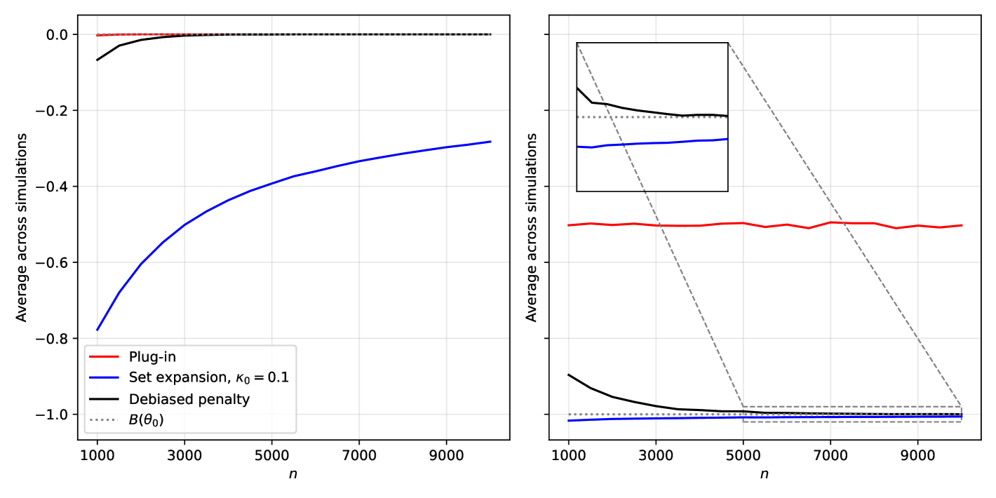
Figure 6: Simulation of example in (14) for $b=-0.05$ and $b=0$ respectively.

Discussion

Consider the right panel of Figure 6, corresponding to $b=0$. The plug-in estimator is inconsistent, while the set-expansion estimator performs well, approaching $-1$ from below for larger $n$. The debiased penalty-function estimator is slightly upward-biased for smaller $n$, but yields the value of almost exactly $-1$ in larger samples. In contrast, the set-expansion estimator has a conservative rate, and remains slightly downward-biased even in larger samples.

The case of $b=-0.05$ is depicted in the left panel of Figure 6. The plug-in estimator is consistent and appears to be the best estimator out of the three. The set-expansion estimator is severely downward-biased. This is because when the optimal vertex has a ‘sharp’ angle, a small expansion of the inequalities’ RHS may lead to a large shift of the vertex. To see that, consider shifting both inequalities outwards in Figure 2 for a small and a large absolute value of $b$, when $b$ is negative. Once the expansion grows smaller, the set-expansion estimator slowly converges to the true value of $0$ from below. While selecting a smaller $\kappa_{0}$ parameter would improve the performance of the set-expansion estimator at $b=-0.05$, in the next part of our analysis we demonstrate that in this example $\kappa_{0}=0.1$ is close to being optimal in the uniform sense, because smaller $\kappa_{0}$ worsens the estimator’s performance at $b=0$. The debiased penalty estimator, in contrast, converges rather quickly. It is slightly conservative at smaller $n$, as it selects the incorrect vertex of $-1$ whenever $\hat{b}_{n}<0$ and $|\hat{b}^{-1}_{n}|>\text{const}\times w_{n}$, i.e. when the penalty parameter is not large enough.

Robustness of the debiased penalty estimator

For $b<0$, the debiased estimator may be expected to perform better at measures with a larger $|b|$. Figure 8 illustrates that point:

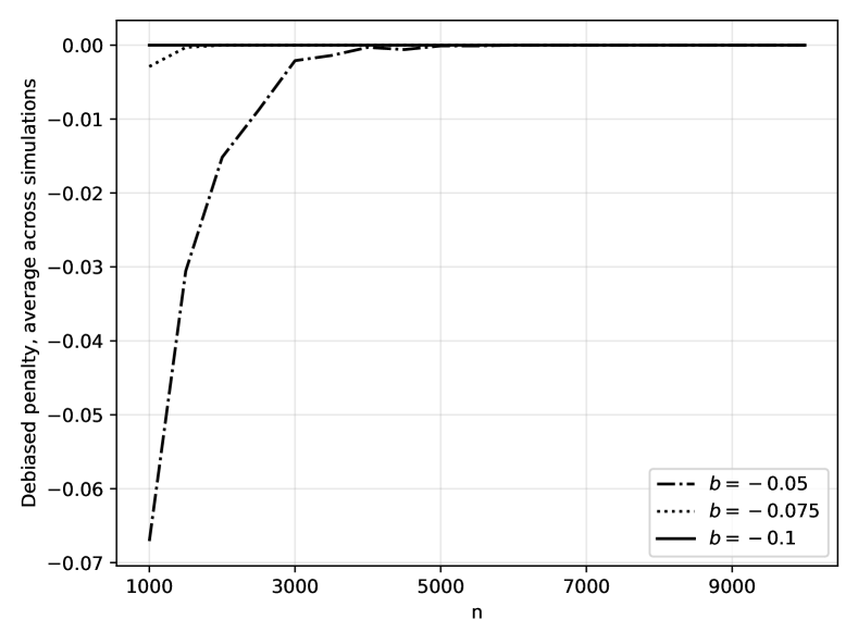
Figure 7: Performance of the debiased penalty estimator for different $b$ in example (14).

Researchers applying any LP estimator should exercise caution when operating in smaller samples due to irregularity inherent in 3. In example (14), the debiased penalty estimator exhibits desirable behavior even along highly irregular measures for sample sizes of order $n=5000$. Such sample sizes are not uncommon in partially identified settings. In our application, estimation is performed on $664633$ observations.

Alternative $\kappa_{0}$

We now investigate to which extent the behavior of the set-expansion estimator can be improved by selecting an alternative $\kappa_{0}$ parameter. Clearly, a larger $\kappa_{n}$ makes the set-expansion estimator more conservative. However, $\kappa_{n}$ cannot be selected as small as possible. If the expansion is too small, it may be insufficient to counteract the noise involved in estimating $\Theta_{I}$, leading to poor performance of the estimator at measures where SC fails to hold.

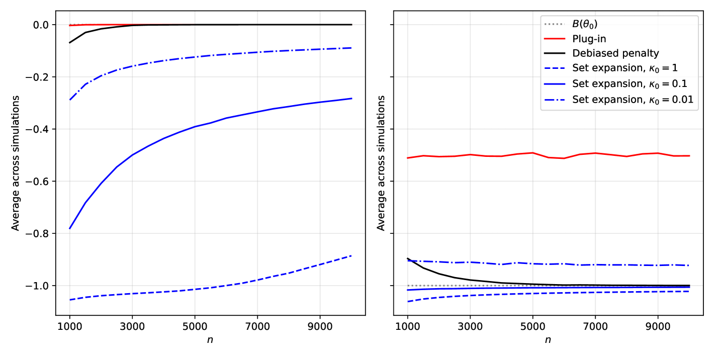
Figure 8: Simulation of (14) for $b=-0.05$ and $b=0$ resp., different $\kappa_{0}$.

That tradeoff is very clear in Figure 8. Compare the performance of the estimator with $\kappa_{0}=0.01$ to the baseline of $\kappa_{0}=0.1$. Decreasing $\kappa_{0}$ down to $0.01$ makes the estimator less conservative at $b=-0.05$, but results in an upward bias at $b=0$. This occurs, because at $\kappa_{0}=0.01$ the resulting set-expansion sequence $\kappa_{n}$ is too small to counteract the estimation noise for the considered sample sizes. This logic is ‘monotone’, meaning that selecting an even smaller $\kappa_{0}$ would worsen the performance at $b=0$ further. Even at $\kappa_{0}=0.01$, the set-expansion estimator is quite conservative for the measure $b=-0.05$, and the parameter can clearly not be reduced any further without affecting the validity of the estimator at $b=0$. It appears that the baseline choice of $\kappa_{0}=0.1$ is close to being optimal in our example. Therefore, the conservative behavior of the set-expansion estimator at $b=-0.05$ is not explained by a poor choice of the tuning parameter, but rather is a feature of the estimator itself.

Noise in $\hat{c}_{n}$

We also report the result of consistency simulations for the DGP described in (15). This DGP features noise on the right-hand-side of the inequalities that describe the polytope, which allows the estimated polytope to be empty.

Figure 9: Simulation of (15) for $b=-0.05$ and $b=0$ resp., different $\kappa_{0}$. Averages for the plug-in and set-expansion estimators ignore failed iterations.

In Figure 9, the plug-in and the debiased penalty estimators perform equally well at $b=-0.05$. The rest of the conclusions are qualitatively unchanged.

2.6.b. Inference

In this section, we assess the performance of our inferential procedure. We compare it to the performance of two recently developed methods, Cho and Russell (2023) (CR) and Gafarov (2024) (BG). We consider a slightly modified version of example (14):

$$M=\begin{pmatrix}-(1+b)&1\\ 1+\zeta&-1\\ 1&0\\ -1&0\end{pmatrix},\quad c=\begin{pmatrix}\nu\\ \zeta\\ -1-\nu\\ -1\end{pmatrix}$$ (15)

The sample analogues $\hat{M}_{n},\hat{c}_{n}$ of parameters in (15) are obtained by substituting $b,\zeta,\nu$ with their estimators:

$$\hat{b}_{n}=b+n^{-1}\sum^{n}_{i=1}U^{b}_{i},\quad\hat{\zeta}_{n}=n^{-1}\sum^{n}_{i=1}U_{i}^{\zeta},\quad\hat{\nu}_{n}=n^{-1}\sum^{n}_{i=1}U_{i}^{\nu},$$

where $U^{k}_{i}\sim U[-0.5;0.5]$, i.i.d. across $i\in[n]$ and $k\in\{b,\zeta,\nu\}$. We consider measures, for which the true values of $\zeta=\nu=0$, whereas we still vary $b$ as in the example before. As before, we mainly consider $b=-0.05$ and $b=0$.

Note that in (15) the plug-in estimator of the polytope $\hat{\Theta}_{I}$ may be empty for some realizations of $\{U^{k}_{i}\}_{i,k}$. That is the case, for example, if $\hat{b}_{n}=\hat{\zeta}_{n}=0$ and $\hat{\nu}_{n}>0$.

Other methods

In case SC fails, the BG estimator is not applicable. It fails to exist in around 25% of cases at $b=0$. The CR estimator in the main text of the paper also relies on $B(\hat{\theta}_{n})$ and is not applicable if SC fails. The procedure described on p.47 of the Supplementary Appendix in Cho and Russell (2023) would not be practically applicable without the results contained in the present paper. It can be shown that the CR augmented procedure combines a random, non-vanishing set expansion and objective function perturbation with the penalty function approach. The authors, however, treat the analogue of the penalty parameter as ‘some [fixed] large value’. They proceed to argue that the inequalities, which establish the size of their inference procedure, hold for any value of $w$, which appears to suggest that its selection is unimportant. There is no practical guidance on $w$ selection, and CR do not implement the augmented estimator in their simulations. In this paper, we studied penalized estimation in great detail, and our results suggest that the appropriate choice of $w$ is critical. Both our previous findings and simulations in Figure 10 demonstrate that for different values of $w$ the performance of the CR procedure ranges from highly conservative to invalid. Selecting ‘a large value’ of $w$ does not yield a valid procedure in finite samples. Our simulations also suggest that CR augmented approach can perform relatively well if combined with our results on the rate and level of $w_{n}$. Unlike our approach, however, it remains asymptotically conservative due to the use of non-vanishing random expansions.

Implementation details

As mentioned in Section 2.2, one can obtain an estimator $\hat{\Sigma}_{n}$ for the asymptotic covariance matrix of $\hat{\theta}_{n}$ via resampling. One then plugs it into the expression for $\sigma(\cdot)$ to obtain the required s.e. An even simpler approach is to obtain an estimator for $\sigma(\hat{A},\hat{x},\hat{v},\Sigma)$ directly by bootstrapping the quantities estimated on the second fold, while keeping the first fold quantities fixed. We have verified that the performance of the two approaches is similar to using the closed-form estimator for $\Sigma$, namely $\hat{\Sigma}_{n}=G\hat{\Omega}_{n}G^{\prime}$, where $G\equiv\frac{\partial\theta}{\partial(b\leavevmode\nobreak\ \zeta\leavevmode\nobreak\ \nu)^{\prime}}$ and $\hat{\Omega}_{n}$ is the sample covariance matrix of $(b_{i}\leavevmode\nobreak\ \zeta_{i}\leavevmode\nobreak\ \nu_{i})^{\prime}$. We employ the latter estimator in our simulations. When implementing the procedure in Cho and Russell (2023) (CR), we use uniform noise with the support size of $0.001$, as recommended in the paper. Note that we refer to their parameter $M$ as $w$. The estimator in Gafarov (2024) (BG) was implemented using the code kindly provided by the author.

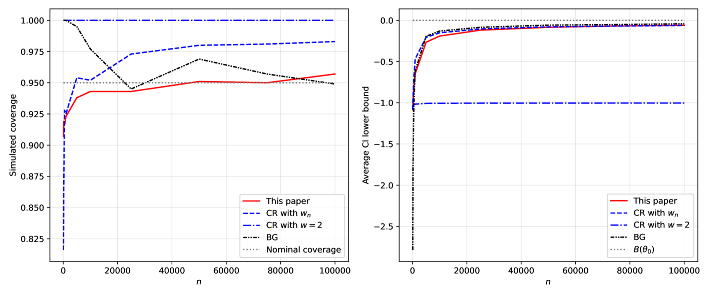
(a) $b=-0.05$. For BG, the number of failed simulations was $206,158,46,6$ at $n=100,200,500,1000$ respectively, none at larger $n$.

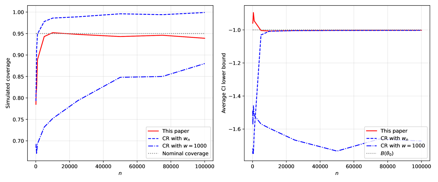
(b) $b=0$. BG omitted, as around $250$ simulations fail.

Figure 10: Performance of different inferential procedures over $1000$ simulations of (15). Left panel - estimated coverage of a $95\%$ one-sided C.I.; right panel - average lower confidence bound.

Discussion

Results of our simulations are given in Figure 10. Overall, it appears that our estimator has the correct nominal level even at smaller sample sizes, whereas the CR with penalty $w_{n}$ overcovers asymptotically. BG estimator achieves nominal coverage asymptotically, although it over-covers in smaller samples and may yield a very conservative left confidence bound, as is evident from the right panel. It fails at $b=0$, because the SC fails. For different fixed values of $w$ the Cho-Russell procedure’s performance may range from highly conservative to invalid. We illustrate this by adding lines with $w=2$ and $w=1000$ to the figures corresponding to $b=-0.05$ and $b=0$, respectively.

3. Special case of LP bounds

Let $Y\in\mathbb{R}$ denote the outcome of interest, $T\in\mathbb{R}$ stand for the treatment, and $Z\in\mathbb{R}^{d_{Z}}$ be the candidate instrument. Here treatment is any variable which effect on $Y$ we attempt to infer, whereas the term instrument refers to an auxiliary variable that allows us to partially identify the causal effect of interest. Our approach nests the case when $Z$ is the usual IV. The reader seeking an economic intuition may refer to Section 5, where $Y$ is the log-wage, $T$ is the level of education, and $Z$ is a proxy for the level of ability.

Denote the supports $Y,T,Z$ as $\mathcal{Y}$, $\mathcal{T}$ and $\mathcal{Z}$ respectively. Throughout this section we consider the case of continuous outcome and discrete treatment and instrument, namely $\mathcal{Y}$ is a (possibly infinite) interval, while $N_{T}\equiv|\mathcal{T}|<\infty$ and $N_{Z}\equiv|\mathcal{Z}|<\infty$. In non-parametric bounds literature it is rather conventional to employ a discrete instrument at the estimation stage (see Manski and Pepper (2009)). While our main identification result may be extended to continuous $Z$, estimation in such settings is left for future research.

Our setup accommodates missing observations of the dependent variable. Namely, we split the set of treatments into two disjoint subsets $\mathcal{T}=\mathcal{O}\sqcup\mathcal{U}$. Whenever $T\in\mathcal{O}$, the researcher observes $Y,T,Z$, whereas if $T\in\mathcal{U}$, only the covariates $T,Z$ are observed. For example, in Blundell et al. (2007) the wage is observed only if an individual is employed. Corresponding to the legs of the treatment are the potential outcomes $Y(t),\leavevmode\nobreak\ t\in\mathcal{T}$:

$$Y=\sum_{t\in\mathcal{O}}\mathds{1}\{T=t\}Y(t)+\sum_{t\in{\mathcal{U}}}\mathds{1}\{T=t\}Y(t)$$

Continuing the wages and education example, the value of $Y(t)$ for a fixed $t\in\mathcal{T}$ may then correspond to the potential wage that an individual with the associated random characteristics would get, had she obtained education $t$.

Let us collect the potential outcomes in the vector $\mathbb{Y}\equiv(Y(t))_{t\in\mathcal{T}}\in\mathbb{R}^{N_{T}}$. Variables $(\mathbb{Y},T,Z,Y)$ are jointly defined on the true probability space $(\mathbb{P},\Omega,\mathcal{S})$ and we let $\mathcal{P}$ denote the considered collection of probability measures on $(\Omega,\mathcal{S})$, such that $\mathbb{P}\in\mathcal{P}$. We impose the following conditions on the set of considered measures throughout this section:

Assumption I0 (Conditions on $\mathcal{P}$).

$\mathcal{P}$ is such that $P\in\mathcal{P}$ if: i) $P$ generates $F_{T,Z}(\cdot)$ and $\{F_{Y|T=t,Z}(\cdot)\}_{t\in\mathcal{O}}$; ii) $P[T=d,Z=z]>0$ $\forall d,z\in\mathcal{T}\times\mathcal{Z}$ and iii) $|\mathbb{E}_{P}[Y(t)|T=d,Z=z]|<\infty$ for all $z\in\mathcal{Z}$ and $t,d\in\mathcal{T}$

Part i) of the Assumption I0 formalizes the assumed identification pattern. It says that the joint distribution of $T,Z$ is always identified and the researcher also observes the joint distribution of $Y,T,Z$ whenever $T\in\mathcal{O}$. Parts ii) and iii) of I0 ensure that all conditional expectations and probabilities are well-defined and finite.

Remark 3.1.

Under no missing data, i.e. $\mathcal{T}=\mathcal{O}$, condition i) is equivalent to $P$ generating the identified joint distribution $F_{Y,T,Z}(\cdot)$.

We define the vector $m$ collecting all elementary conditional moments as

$$m(P)\equiv(\mathbb{E}_{P}[\mathbb{Y}|T=d,Z=z])_{d\in\mathcal{T},z\in\mathcal{Z}}\in\mathbb{R}^{N^{2}_{T}N_{Z}},$$

and suppose that the researcher is interested in the target parameter $\beta^{*}$, given by

$$\beta^{*}=\mu^{*}(\mathbb{P})^{\prime}m(\mathbb{P}),$$ (16)

where $\mu^{*}:\mathcal{P}\to\mathbb{R}^{N^{2}_{T}N_{Z}}$ is identified and chosen by the researcher. It parametrizes the choice of the outcome of interest, as the following remark clarifies.

Remark 3.2.

The form (16) nests i) $\mathbb{E}[Y(t)]$, ii) $ATE_{td}=\mathbb{E}[Y(t)-Y(d)]$ and iii) $CATE_{td,A,B}=\mathbb{E}[Y(t)-Y(d)|T\in A,Z\in B]$.

3.1. Affine inequalities over conditional moments

We now introduce the general class of identifying conditions described by affine inequalities over conditional moments, potentially augmented with affine a.s. restrictions. These restrict the set of admissible measures to $\mathcal{P}^{*}$:

$$\mathcal{P}^{*}\equiv\{P\in\mathcal{P}|(M^{*}m+b^{*})(P)\geq 0\land(\tilde{M}\mathbb{Y}+\tilde{b})(P)\geq 0\text{\leavevmode\nobreak\ $P$-a.s.}\},$$ (17)

where $b^{*}:\mathcal{P}\to\mathbb{R}^{R}$, $M^{*}:\mathcal{P}\to\mathbb{R}^{R\times N^{2}_{T}N_{Z}}$, $\tilde{b}:\mathcal{P}\to\mathbb{R}^{\tilde{R}}$ and $\tilde{M}:\mathcal{P}\to\mathbb{R}^{\tilde{R}\times N_{T}}$ are identified parameters, chosen by the researcher. These parametrize the choice of $R\in\mathbb{N}$ identifying inequalities on conditional moments of potential outcomes as well as $\tilde{R}\in\mathbb{N}$ almost sure inequalities on the potential outcomes. In general, $\psi(P)\equiv(\mu^{*}(P),b^{*}(P),M^{*}(P),\tilde{b}(P),\tilde{M}(P))$ and $m(P)$ are functionals of $P$. We omit this dependence whenever it does not cause confusion.

The family of models that can be written in the form (17) is very rich, as illustrated by the following examples.

Example 3.1 (MIV).

$Z\in\mathbb{R}$ is a monotone IV Manski and Pepper (2000) if, for each $t\in\mathcal{T}$ and $z,z^{\prime}\in\mathcal{Z}$, if $z^{\prime}\geq z$, then $\mathbb{E}[Y(t)|Z=z^{\prime}]\geq\mathbb{E}[Y(t)|Z=z]$. MIV is nested in AICM for an appropriate choice of matrix $M^{*}=M_{MIV}$ and $b^{*}=0$, and no a.s. restrictions, $\tilde{M}=0,\leavevmode\nobreak\ \tilde{b}=0$. Monotone treatment selection assumption in Manski and Pepper (2000) obtains under $Z=T$.

Example 3.2 (IV).

$Z\in\mathbb{R}$ is mean-independent of potential outcomes if, for each $t\in\mathcal{T}$ and $z,z^{\prime}\in\mathcal{Z}$, $\mathbb{E}[Y(t)|Z=z^{\prime}]=\mathbb{E}[Y(t)|Z=z]$. This assumption is nested in AICM for $M^{*}=M_{IV}\equiv(M^{\prime}_{MIV}\quad-M^{\prime}_{MIV})^{\prime}\leavevmode\nobreak\$, $b^{*}=0$, and no a.s. restrictions.

Example 3.3 (MTR).

Monotone treatment response assumption Manski and Pepper (2000) imposes that, for each $t,t^{\prime}\in\mathcal{T}$, if $t^{\prime}>t$, then $Y(t^{\prime})\geq Y(t)$ a.s. It is nested in AICM for an appropriate choice of matrix $\tilde{M}=\tilde{M}_{MTR}$ with $\tilde{b}=0$, and no inequalities over conditional moments, $M^{*}=0,\leavevmode\nobreak\ b^{*}=0$.

Example 3.4 (Roy model).

Lafférs (2019) imposes that for each $t,z\in\mathcal{T}\times\mathcal{Z}$, the individual’s choice is, on average, optimal: $\mathbb{E}[Y(t)|T=t,Z=z]=\max_{d\in\mathcal{T}}\leavevmode\nobreak\ \mathbb{E}[Y(d)|T=t,Z=z]$. It is nested for an appropriate choice of matrix $M^{*}=M_{ROY}$ and $b^{*}=0$, and no a.s. restictions.

Example 3.5 (Missing data).

Blundell et al. (2007) derives bounds on $F(w|x)$ - the cdf of wages evaluated at some $w\in\mathbb{R}$, conditional on $X=x$. The wage is observed if the individual is employed, $E=1$, and unobserved otherwise ($E=0$). Introduce $\mathcal{O}=\{1\}$ and $\mathcal{U}=\{0\}$. Let $Y(t)\equiv\mathds{1}\{W\leq w\}$, so that $\mathbb{E}[Y(t)|X=x]=F(w|x)$. Our approach allows to accommodate all identifying conditions in the original paper by appropriately choosing $M^{*},b^{*}$ and $\tilde{M},\tilde{b}$.

Remark 3.3.

Combinations of assumptions are obtained by stacking the respective matrices, as in Example 3.2. Sensitivity analysis can be performed via relaxations $b_{\ell}^{*}=b^{*}+\ell$, or $\tilde{b}_{\ell}=\tilde{b}+\ell$ for some $\ell\geq 0$. For example, given some $\ell=\{\ell(t,z,z^{\prime})\}_{t,z,z^{\prime}}\geq 0$, inequalities $\mathbb{E}[Y(t)|Z=z^{\prime}]-\mathbb{E}[Y(t)|Z=z]\geq-\ell(t,z,z^{\prime})$ for $z,z^{\prime}\in\mathcal{Z}$ with $z^{\prime}>z$ and $t\in\mathcal{T}$ yield a relaxation of MIV. In De Haan (2017) the shape of observed moments may suggest a failure of monotonicity near the boundaries of $\text{Supp}(Z)$. Selecting positive $\ell(z,z^{\prime})$ for values of $z,z^{\prime}$ close to the boundaries could constitute a meaningful robustness check.

3.2. Linear programming bounds

We now provide the general identification result for the models described by $\mathcal{P}^{*}$. Let us construct $x$ that collects unobserved pointwise-conditional moments and the vector $\overline{x}$ of those pointwise-conditional moments that are identified:

$$x \equiv(\mathbb{E}[Y(t)|T=d,Z=z])_{z\in\mathcal{Z}\land(t,d\in\mathcal{T}:t\neq d\lor t,d\in\mathcal{U}:t=d)},$$

$$\overline{x} \equiv(\mathbb{E}[Y(t)|T=t,Z=z])_{z\in\mathcal{Z},t\in\mathcal{O}}.$$

For known selector matrices $P_{m},\overline{P}_{m}$, one can then decompose $m$ as

$$m=\underbrace{P_{m}x}_{\text{partially identified}}+\underbrace{\overline{P}_{m}\overline{x}}_{\text{identified}}.$$

It is also straightforward to observe that $\tilde{M}\mathbb{Y}+\tilde{b}\geq 0$ a.s. implies

$$(I_{N_{T}N_{Z}}\otimes\tilde{M})m+\iota_{N_{T}N_{Z}}\otimes\tilde{b}\geq 0.$$ (18)

Before we state the main identification result, let us construct the matrix $M^{**}$ and the vector $b^{**}$ that combine the conditional restrictions with the implications of the almost sure restrictions in (18), as

$$M^{**}\equiv\begin{pmatrix}I_{N_{T}N_{Z}}\otimes\tilde{M}\\ M^{*}\end{pmatrix},\quad b^{**}\equiv\begin{pmatrix}\iota_{N_{T}N_{Z}}\otimes\tilde{b}\\ b^{*}\end{pmatrix}.$$ (19)

Suppose Assumption I0 holds. For any $\psi$, the sharp identified set $\mathcal{B}^{*}$ for $\beta^{*}$ satisfies

$$\mathcal{B}^{*}\equiv(\mu^{*\prime}m)(\mathcal{P}^{*})\subseteq\{\beta\in\mathbb{R}|\underset{x:Mx\geq c}{\inf}p^{\prime}x\leq\beta-\overline{p}^{\prime}\overline{x}\leq\underset{x:Mx\geq c}{\sup}p^{\prime}x\},$$ (20)

where

$$\overline{p}\equiv\overline{P}^{\prime}_{m}\mu^{*},\quad p\equiv P^{\prime}_{m}\mu^{*},\quad M\equiv M^{**}P_{m},\quad c\equiv-b^{**}-M^{**}\overline{P}_{m}\overline{x}.$$

Reverse inclusion in (20) holds if $\tilde{M}=0,\tilde{b}=0$, or if one of the following is true:

1. MTR holds, i.e. $Y(t_{1})\geq Y(t_{0})$ a.s. $\forall t_{1},t_{0}\in\mathcal{T}$ s.t. $t_{1}>t_{0}$:

   $$\tilde{M}=\tilde{M}_{MTR},\quad\tilde{b}=0_{N_{T}-1}$$

2. Outcomes are bounded, $Y(t)\in[K_{0};K_{1}]$, $\forall t\in\mathcal{T}$ a.s. for known $K_{1}>K_{0}$:

   $$\tilde{M}=\tilde{M}_{b}\equiv\begin{pmatrix}I_{N_{T}}\\ -I_{N_{T}}\end{pmatrix},\quad\tilde{b}=\tilde{b}_{b}\equiv\begin{pmatrix}-K_{0}\cdot\iota_{N_{T}}\\ K_{1}\cdot\iota_{N_{T}}\end{pmatrix}.$$ (21)

3. MTR holds, outcomes are bounded and $(\Omega,\mathcal{S})$ can support a $U[0;1]$ r.v.:

   $$\tilde{M}=\begin{pmatrix}\tilde{M}_{MTR}\\ \tilde{M}_{b}\end{pmatrix},\quad\tilde{b}=\begin{pmatrix}\tilde{b}_{MTR}\\ 0_{N_{T}-1}\end{pmatrix}.$$ (22)

The matrix $\tilde{M}_{MTR}$ is defined in Appendix D.3.

Theorem 3.2 postulates that bounds on the target parameter $\beta^{*}$ under $\mathcal{P}^{*}$ can be obtained by solving two linear programs. The LP bounds are sharp if there are no a.s. inequalities in the model, or if the a.s. inequalities parametrize three special cases that are typically used in the literature. Otherwise, the LP bounds are valid, but not necessarily sharp, as we show in Appendix D.2. This is because, in general, the entire distribution of $\mathbb{Y},T,Z$ is relevant for $\beta^{*}$ under a.s. restrictions. The naive approach of searching over such joint distributions, however, would involve infinite-dimensional optimization, because $|\mathcal{Y}|=\infty$.

Remark 3.4.

We are not aware of affine a.s. restrictions $\tilde{M},\tilde{b}$ used in applied work that are not special cases 1-3 in Theorem 3.2. The special cases 1-3 appear in Blundell et al. (2007), Kreider et al. (2012), Gundersen et al. (2012), Siddique (2013).

Remark 3.5.

The empirical literature has extensively relied on the MIV + MTR + MTS combination of Manski and Pepper (2000) assumptions, as it yields the tightest bounds out of all classical conditions. In the absence of a theoretical justification, this has led to errors Lafférs (2013). Theorem 3.2 provides the first available sharp bounds under this combination when $Y$ is continuous.

Remark 3.6.

In any of the sharp cases in Theorem 3.2, the polytope $\Theta_{I}\equiv\{x\in\mathbb{R}^{q}:Mx\geq c\}$ gives the sharp identified set for the vector of unobserved pointwise-conditional moments $x$ under the corresponding AICM model described by $M,c$.

4. Conditional monotonicity assumptions

A particular family of identifying conditions that can be written in the form (17) is the conditional monotonicity class of assumptions. These impose that potential outcomes are mean-monotone in the instrument even within some treatment subgroups. While more restrictive than the conventional MIV, conditionally monotone instrumental variables (cMIV) allow to sharpen the bounds on the outcomes of interest. Throughout this section, we assume that outcomes are bounded $Y(t)\in[K_{0};K_{1}]\leavevmode\nobreak\ a.s.$ for known $K_{0},K_{1}\in\mathbb{R}$, $K_{0}<K_{1}$. We also suppose that there are no missing data, i.e. $\mathcal{T}=\mathcal{O}$.

We argue that cMIV assumptions are reasonable in classical applications, discuss the difference between MIV and cMIV and develop a formal testing strategy for a particular version of cMIV. This testing procedure relies on the observed outcomes’ monotonicity, which has been typically used in applied work to justify applying MIV. Our results imply that if such monotonicity is observed and the researcher is comfortable with MIV, the cMIV assumption is inexpensive, and can be applied to sharpen the bounds on the outcomes of interest. In some applications, as is the case in Section 5, cMIV yields informative bounds even when the classical conditions fail to do so.

While we only discuss three variations of cMIV, the class of such assumptions is potentially richer, and Theorem 3.2 applies in any such framework.

Assumption cMIV-s.

Suppose that for any $t\in\mathcal{T}$, $A\subseteq\mathcal{T}:A\neq\{t\}$ and $z,z^{\prime}\in\mathcal{Z}$ s.t. $z^{\prime}>z$ we have:

$$\mathbb{E}[Y(t)|T\in A,Z=z^{\prime}]\geq\mathbb{E}[Y(t)|T\in A,Z=z],$$

i.e. the potential outcomes are, on average, non-decreasing in $Z$ for any treatment subgroup.

The strong conditional monotonicity assumption possesses the greatest identifying power across all considered cMIV conditions. To see that cMIV-s implies MIV, set $A=\mathcal{T}$ in the definition above.

Assumption cMIV-w.

Suppose MIV holds and for any $t\in\mathcal{T}$ and $z,z^{\prime}\in\mathcal{Z}$ s.t. $z^{\prime}>z$ we have:

$$\mathbb{E}[Y(t)|T\neq t,Z=z^{\prime}]\geq\mathbb{E}[Y(t)|T\neq t,Z=z],$$

i.e. the potential outcomes are, on average, non-decreasing in $Z$ for the non-treated and the whole population.

The weak conditional monotonicity assumption allows for closed-form expressions for sharp bounds that are easy to compute and perform inference on.

Assumption cMIV-p.

Suppose MIV holds and for any $t\in\mathcal{T},d\in\mathcal{T}\setminus\{t\}$ and $z,z^{\prime}\in\mathcal{Z}$ s.t. $z^{\prime}>z$ we have:

$$\mathbb{E}[Y(t)|T=d,Z=z^{\prime}]\geq\mathbb{E}[Y(t)|T=d,Z=z],$$

i.e. the potential outcomes are, on average, non-decreasing in $Z$ conditional on any counterfactual level of treatment.

The pointwise conditional monotonicity assumption is directly testable under a mild homogeneity condition, see Section 4.2.

Conditional monotonicity restrictions differ in the collection of treatment subsets over which monotonicity in the instrument is assumed. The strong conditionally monotone instruments are such that, among individuals from any given counterfactual treatment subgroup, higher values of $Z$ are, on average, associated with higher potential outcomes. The weak conditional monotonicity restriction only imposes the same mean-monotonicity on the whole population and on the untreated, whereas the pointwise form assumes it over the entire population as well as conditional on each counterfactual level of treatment.

Remark 4.1.

All cMIV assumptions imply MIV. Moreover, cMIV-w, cMIV-p are implied by cMIV-s. If treatment is binary, cMIV-s, cMIV-w and cMIV-p are equivalent.

While it is possible for the general apporach of form (17), cMIV conditions avoid assuming monotonicity over the observed treatment subset $\{T=t\}$. This is because such monotonicity is identified. If it holds, it should not add any identifying power to our conditions in theory. However, large violations of the observed outcomes’ monotonicity will lead the test developed in Section 4.2 to reject cMIV-p and cMIV-s.

The following observation motivates the use of cMIV assumptions.

Manski and Pepper (2000) MIV bounds are not sharp under either cMIV-s, cMIV-w or cMIV-p.

Proof.

Consider a binary treatment $T$, three levels of the instrument $Z\in\{z_{0},z_{1},z_{2}\}$ with $z_{0}<z_{1}<z_{2}$ and $-K_{0}=K_{1}=1$. Suppose for a fixed $t\in\{0,1\}$, we have $\mathbb{E}[Y(t)|T=t,Z=z_{i}]=0$, with $P[T\neq t|Z=z_{0}]=0.125$, $P[T\neq t|Z=z_{1}]=0.5$, $P[T\neq t|Z=z_{2}]=0.25$. The no-assumptions lower bounds on $\mathbb{E}[Y(t)|Z=z_{i}]$ are $(-0.125,\leavevmode\nobreak\ -0.5,\leavevmode\nobreak\ -0.25)$. MIV ‘irons’ the no-assumptions bounds to $(-0.125,\leavevmode\nobreak\ -0.125,\leavevmode\nobreak\ -0.125)$, which also implies the lower bounds on $\mathbb{E}[Y(t)|T\neq t,Z=z_{i}]$: $(-1,\leavevmode\nobreak\ -0.25,\leavevmode\nobreak\ -0.5)$. Under cMIV, one can further ‘iron’ these to improve the lower bound for $z_{2}$ up to $-0.25$, so that the lower bound on $\mathbb{E}[Y(t)|Z=z_{2}]$ becomes $-1/16>-1/8$. ∎

Sharp bounds for all versions for cMIV follow from Theorem 3.2. We also show that under cMIV-w the bounds can be characterized explicitly, which is especially convenient if the treatment is binary, so that all cMIV assumptions coincide (see Appendix I.1). For didactic purposes, we also provide detailed guidance on how to construct the triplet $M,c,p$ from Theorem 3.2 under cMIV-s, cMIV-p and MIV in Appendix I.2.

4.1. Discussion of cMIV

This section illustrates the difference between MIV and cMIV by considering two parametric examples with classical applications.

4.1.a. Education selection

Consider the following empirical setup. Suppose $T$ is an indicator of whether or not an individual has a university degree, $Y(t)$ are potential log wages and $Z$ is an observed indicator of ability.

MIV assumption on $Z$ implies that more able individuals can do better both with and without a college degree on average: $\mathbb{E}[Y(t)|Z=z]$ - monotone in $z$. cMIV additionally imposes that: i) among those who have a college degree, a smarter individual could have done relatively better on average than their counterpart if both did not have it: $\mathbb{E}[Y(0)|Z=z,T=1]$ - monotone in $z$; and ii) among those who do not have a college degree, a smarter individual could have done relatively better on average than their counterpart if both had it: $\mathbb{E}[Y(1)|Z=z,T=0]$ - monotone in $z$.

We now consider a parametric example. Suppose that $\eta$ measures how diligent one is from birth and is ex-ante mean-independent of $Z$. While $Z$ is observed by both the employers and the econometrician (e.g. an IQ score), the employer additionally observes the employee effort level $\eta+\varepsilon$ with $\varepsilon\rotatebox[origin={c}]{90.0}{$\models$}(Z,T,\eta)$. Suppose $Var(Z)=Var(\eta)=1$ and $\mathbb{E}[Z]=\mathbb{E}[\eta]=\mathbb{E}[\varepsilon]=0$. Suppose that, on average, employees choose $T$ to maximize their expected earnings. This motivates a stylized Roy selection model, with

$$Y(t)=\beta_{0}(t)+\beta_{1}(t)Z+\beta_{2}(t)\eta+\varepsilon(t),\quad T=\mathds{1}\{\mathbb{E}[Y(1)-Y(0)|Z,\eta]+\nu\geq 0\},$$

where $\nu\rotatebox[origin={c}]{90.0}{$\models$}(Z,\eta,\varepsilon)$ is remaining heterogeneity, and $\varepsilon(t)\equiv\beta_{2}(t)\varepsilon$. MIV demands that

$$(\text{MIV}):\beta_{1}(t)\geq 0.$$

MIV postulates that the direct effect of ability on potential earnings is positive. It seems reasonable to suppose that $\beta_{i}(t)\geq 0,\leavevmode\nobreak\ i=1,2,\leavevmode\nobreak\ t=0,1$, i.e. both effort and ability increase potential wages. Letting $\delta_{z}\equiv\beta_{1}(1)-\beta_{1}(0)$ and $\delta_{\eta}\equiv\beta_{2}(1)-\beta_{2}(0)$ denote the differentials in the effects of ability and effort respectively, the additional requirement of cMIV is that:

$$\underbrace{\beta_{1}(0)z}_{\text{direct effect}}+\underbrace{\beta_{2}(0)\mathbb{E}[\eta|\delta_{z}z+\delta_{\eta}\eta+\tilde{\nu}\geq 0]}_{\text{selection given $T=1$}}-\text{increasing}$$ (23)

$$\underbrace{\beta_{1}(1)z}_{\text{direct effect}}+\underbrace{\beta_{2}(1)\mathbb{E}[\eta|\delta_{z}z+\delta_{\eta}\eta+\tilde{\nu}\leq 0]}_{\text{selection given $T=0$}}-\text{increasing},$$ (24)

where $\tilde{\nu}\equiv\beta_{0}(1)-\beta_{0}(0)+\nu$.

Notice that if $\delta_{z}$ and $\delta_{\eta}$ are of different signs, for example because the jobs that one may apply for with a college degree are more ability-intensive ($\delta_{z}>0$), whereas those which are available otherwise are more skill-intensive ($\delta_{\eta}<0$), the additional conditional monotonicity requirements (23)-(24) are less strict than MIV. This is because, conditional on both having a degree and not having it, ability and effort are positively associated.

Intuitively, among those who do not have a degree ($T=0$), people of higher ability must have had stronger incentives to forgo college. This should have been because a higher level of diligence gives them a comparative advantage in effort-intensive jobs. Among those with a degree, higher ability implies a comparative advantage in ability-intensive occupations, which explains their willingness to select into this option ($T=1$). It does not, therefore, signal as low an effort level as it would for a less capable individual.

Now consider the same setup with $\delta_{z}=\delta_{\eta}>0$ and $\tilde{\nu}=0$,

$$T=\mathds{1}\{\eta+Z\geq 0\}.$$

This selection mechanism can be explained by the fact that to get a degree one needs to be either hard-working or of high ability. The requirement of MIV is unchanged, and cMIV necessitates that:

$$\beta_{1}(0)z+\beta_{2}(0)\mathbb{E}[\eta|\eta\geq-z]-\text{increasing}$$ (25)

$$\beta_{1}(1)z+\beta_{2}(1)\mathbb{E}[\eta|\eta\leq-z]-\text{increasing}$$ (26)

In this case, conditional on each level of education, effort level $\eta$ and ability $Z$ are negatively associated, so the conditional selection terms in (25)-(26) make cMIV a stricter assumption than MIV. Intuitively, a more able individual with a college degree did not need to work as hard to get it as her counterpart with a lower ability. Similarly, if an individual is capable, but does not have a degree, she has to be of lower effort as otherwise she would have selected into education.

Even if MIV holds, cMIV can thus fail if employer prefers effort over ability to the extent that the conditional negative association between the two outweighs the direct impact of ability on wages as well as any ex-ante positive correlation between the employer-observed signal of diligence and the ability.

An examination of equations (23) and (24) suggests that cMIV is more likely to hold whenever $\delta_{z}$ is small relative to $\delta_{\eta}$, while $\beta_{1}(\cdot)$ is large relative to $\beta_{2}(\cdot)$. This means that $Z$ should be relatively weak in the parlance of the classical IV models, and strongly monotone.

Overall, it seems reasonable to use a proxy for the level of ability as a conditionally monotone instrument in the estimation of returns to schooling. One would be inclined to think that while $Z$ does enter selection, it affects the potential outcomes directly and strongly enough, so that there are no subgroups by schooling for which a higher value of ability would correspond to lower potential wages on average.

4.1.b. Simultaneous equations

As some aspects of mathematical intuition may be muted in discrete models, we also consider a simple continuous setup to confirm the insights derived from the previous analysis. For illustrative purposes, we drop the boundedness and discreteness assumptions and consider the supply and demand simultaneous equations,

$$q^{k}(p)=\alpha^{k}(p)+\beta^{k}(p)Z+\gamma^{k}(p)\eta+\kappa^{k}(p)\varepsilon^{k},\leavevmode\nobreak\ k\in\{s,d\}.$$

The observed log-price $P$ clears the market in expectation,

$$P\in\{p\in\mathbb{R}|\mathbb{E}[q^{s}(p)|Z,\eta]=\mathbb{E}[q^{d}(p)|Z,\eta]\},$$ (27)

where $\eta,Z$ are continuous unobserved and observed random variables respectively, with $\mathbb{E}[\eta|Z]=0$ a.s. and $\mathbb{E}[\varepsilon^{k}]=0$ with $\varepsilon^{k}\rotatebox[origin={c}]{90.0}{$\models$}(\eta,Z,\varepsilon^{-k})$ for $k\in\{s,d\}$. Further assume that all functions of $p$ are continuous.

Potential price $p$ indexes the potential outcomes, giving rise to the demand and supply schedules. Suppose we aim to identify the elasticity of supply, $\mathbb{E}[(q^{s}(p_{1})-q^{s}(p_{0}))/(p_{1}-p_{0})]$ for some $p_{1}>p_{0}$, and $Z$ is a monotone instrument for $q^{s}(p)$, while $P$ can be interpreted as treatment. $\eta$ is unobserved heterogeneity and $\varepsilon^{k}$ are random violations from the market clearing condition or measurement errors independent of the rest of the model. For an individual realization of market clearing an econometrician observes $\{P,\{q^{k}(P)\}_{k},Z\}$, but does not observe the schedules at other prices $\{q^{k}(p)\}_{k}\text{ for }p\neq P$, nor disturbances $\{\eta,\{\varepsilon^{k}\}_{k}\}$.

Define $\delta_{z}(p)\equiv\beta^{s}(p)-\beta^{d}(p)$ and similarly for $\eta$, with $\delta_{p}(p)\equiv\alpha^{s}(p)-\alpha^{d}(p)$. As stated, the model is potentially incomplete or incoherent, as for a given vector $(Z,\eta)$ equation (27) may have multiple or no solutions. To avoid that, so long as that the support of $Z,\eta,\varepsilon^{k}$ is full, it is necessary that $\delta_{z}(p)$, $\delta_{\eta}(p)$ be constant. We shall assume that for simplicity. Provided that $\delta_{p}(p)$, which determines the excess supply at fixed $(Z,\eta)$, is strictly increasing and has full image, the model is complete and coherent, and

$$P=\delta^{-1}_{p}(-\delta_{z}Z-\delta_{\eta}\eta).$$ (28)

Equation (28) introduces a deterministic linear relationship between $Z$ and $\eta$ conditional on each given value of $P$. As we saw in the previous example, this constitutes the worst-case scenario for cMIV, if $\delta_{z}$ and $\delta_{\eta}$ have the same sign. A noisier selection mechanism would relax the conditional link between $Z$ and $\eta$, and would thus weaken the conditional selection channel.

Note that the reduced-form error is $u\equiv\gamma^{s}(P)\eta+\kappa^{s}(P)\varepsilon^{s}$ and there is a simultaneity bias, as

$$\mathbb{E}[Pu]=\mathbb{E}[P\gamma^{s}(P)\underbrace{\mathbb{E}[\eta|\delta_{z}Z+\delta_{\eta}\eta=P]}_{\text{simultaneity/ommited variable}}]\neq 0.$$

In this setup, MIV requires that

$$(\text{MIV}):\leavevmode\nobreak\ \beta^{s}(p)\geq 0,\leavevmode\nobreak\ \forall p\in\mathbb{R}.$$

Whereas cMIV-p additionally imposes that

$$\beta^{s}(p)z+\gamma^{s}(p)\mathbb{E}[\eta|\delta_{z}z+\delta_{\eta}\eta=-\delta_{p}(d)]\geq 0-\text{increasing in}\leavevmode\nobreak\ z,\leavevmode\nobreak\ \forall p,d\in\mathbb{R}:d\neq p.$$ (29)

Suppose that $\delta_{z},\delta_{\eta}\neq 0$ to rule out uninteresting cases. (29) then implies

$$\beta^{s}(p)\geq\gamma^{s}(p)\frac{\beta^{s}(p)-\beta^{d}(p)}{\gamma^{s}(p)-\gamma^{d}(p)}.$$ (30)

For concreteness, consider two positive supply shocks, i.e. $\beta^{s}(p),\gamma^{s}(p)>0$. Equation (30) means that either $\eta$ and $Z$ affect the reduced-form equilibrium price in different directions (recall the comparative advantage example), or the effect of $Z$ on the equilibrium price relative to its effect on the supply schedule is smaller than that of $\eta$,

$$\text{sgn}(\delta_{\eta})\neq\text{sgn}(\delta_{z})\quad\text{or}\quad\left|\frac{\beta^{s}(p)-\beta^{d}(p)}{\beta^{s}(p)}\right|\leq\left|\frac{\gamma^{s}(p)-\gamma^{d}(p)}{\gamma^{s}(p)}\right|.$$ (31)

Under $\text{sgn}(\delta_{\eta})=\text{sgn}(\delta_{z})$, equation (31) once again requires that $Z$ be strongly monotone and relatively weak for cMIV-p to hold. The logic we described may help the researcher navigate the potential economic forces in a given application to decide whether cMIV-p is a suitable assumption.

For example, consider estimating the supply elasticity in the market for plane tickets in the early days of Covid-19 pandemic. Suppose $Z$ is an inverse Covid-stringency index for the economy, while $\eta$ may be interpreted as residual cost shocks, defined to be mean-independent of $Z$. It is likely that $\delta_{\eta}\approx\gamma^{s}$, i.e. residual cost shocks affect mainly the supply in that sector, and not the demand. It is also likely that either supply is less responsive to $Z$ than demand (so that cMIV is implied by MIV), or the effects are of the same order of magnitude. $Z$ is therefore likely to be a conditionally monotone instrument.

4.2. Testing cMIV

One could argue against cMIV conditions whenever $\mathbb{E}[Y(t)|T=t,Z=z]$ fail to be monotone in the data. In general, the power and size of that test are unclear. There is, however, a special case when cMIV can be tested directly, provided that the researcher is willing to assume MIV. In some applications one may conjecture that the potential outcomes’ functions $Y(t)$, either in the reduced or in the structural form, are such that the relative effects of $Z$ and the unobserved variable(s) $\eta$, potentially correlated with $Z$, are unchanged across outcome indices $t$.

Researchers often impose even stricter versions of this homogeneity assumption. For example, Manski and Pepper (2009) discuss MIV identification under HLR condition: $Y(t)=\beta t+\eta$. Conditions in Proposition 4.2 relax HLR to an arbitrary shape of response of a potential outcome to treatment and allow for a generally heteroscedastic/treatment-specific response to unobserved variables and instrument, so long as the relative effects are unchanged across potential outcomes. All functions in the proposition below are assumed to be measurable.

Suppose that a): i) $Y(t)=g(t,\xi)+h(t)\psi(Z,\eta)$, $h(t)\neq 0$ for all $t\in\mathcal{T}$, with $\xi\rotatebox[origin={c}]{90.0}{$\models$}(T,Z,\eta)$ and ii) MIV holds, strictly for some $z,z^{\prime}\in\mathcal{Z}$ with $z^{\prime}>z$; or b): i) $Y(t)=g(t,\xi,T)+h(t)\psi(Z,\eta)$ for all $t\in\mathcal{T}$, with $\xi\rotatebox[origin={c}]{90.0}{$\models$}(T,Z,\eta)$, ii) $\frac{h(t)}{h(d)}>0\leavevmode\nobreak\ \forall t,d\in\mathcal{T}$; and iii) MIV holds. Then Assumption cMIV-p holds iff $\mathbb{E}[Y(t)|T=t,Z=z]$ are all monotone. Note that whether or not $h(t)\neq 0$ is observable in the data for case $(a)$ and whether or not $h(t)/h(d)>0$ is also identified for $(b)$.

Remark 4.2.

The monotonicity of observed outcomes has been routinely used in applied work to motivate the use of MIV condition (e.g. De Haan (2017)). We show that, given that MIV holds and under a homogeneity condition, the observed monotonicity is instead equivalent to cMIV-p.

Remark 4.3.

cMIV is testable in Example 4.1.b because the reduced form expression has the form $b):i)$. It is testable in Example 4.1.a if instead of separately observing $\eta,Z$, employers on average observe a mixed signal of ability and effort, $s\equiv aZ+b\eta$ for some $a,b\in\mathbb{R}$.

A test of cMIV-p is thus the test of all $f_{t}(z)\equiv\mathbb{E}[Y(t)|T=t,Z=z]$ being monotone,

$$\mathcal{H}_{0}:f_{t}(z)-\text{increasing in }z,\leavevmode\nobreak\ \forall t\in\mathcal{T}.$$

To obtain such a test, we may extend the procedure in Chetverikov (2019). Denote the set of all observations with treatment level $t$ as $\mathcal{I}_{t}\equiv\{i\in[n]:T_{i}=t\}$ with $n_{t}\equiv|\mathcal{I}_{t}|$. Suppose $\phi^{t}_{n_{t}}$ is the corresponding Chetverikov’s regression monotonicity test (or a corresponding parametric test for discrete $Z$) with the confidence level $\alpha_{t}\in(0;0.5)$. We define the joint test as

$$\phi_{n}\equiv\max_{t\in\mathcal{T}}\leavevmode\nobreak\ \phi^{t}_{n_{t}}.$$

Denote $\mathcal{P}^{C}$ to be the set of probability measures, such that for all $P\in\mathcal{P}^{C}$ and all $t\in\mathcal{T}$ the conditional probability measure given $T=t$ that $P$ generates satisfies the regularity conditions in Theorem 3.1 in Chetverikov (2019). Similarly, let $\mathcal{P}^{C}_{t}$ be the set of all the conditional probability measures given $T=t$ that measures from $\mathcal{P}^{C}$ generate.

If $\Pi_{t\in\mathcal{T}}(1-\alpha_{t})\geq 1-\alpha$, then

$$\inf_{P\in\mathcal{P}^{C}\cap\mathcal{H}_{0}}\leavevmode\nobreak\ P[\phi_{n}=0]\geq 1-\alpha+o(1),$$

as $n\to\infty$.

Proof.

Notice that each $\phi^{t}_{n_{t}}$ is a function of the observations from $\mathcal{I}_{t}$ only. Since $\mathcal{I}_{t}$ are mutually exclusive by construction and because the data are i.i.d., we have $P[\phi_{n}=0]=\Pi_{t\in\mathcal{T}}P[\phi^{t}_{n_{t}}=0]$. By the standard optimization argument, we have

$$\Pi_{t\in\mathcal{T}}\underset{P\in\mathcal{P}_{t}^{C}}{\inf}\leavevmode\nobreak\ P[\phi^{t}_{n_{t}}=0]\leq\underset{P\in\mathcal{P}^{C}}{\inf}\Pi_{t\in\mathcal{T}}P[\phi^{t}_{n_{t}}=0].$$

Theorem 3.1 from Chetverikov (2019) and $\Pi_{t\in\mathcal{T}}(1-\alpha_{t})\geq 1-\alpha$ then yield the result. ∎

Remark 4.4.

One may set $\alpha_{t}=1-(1-\alpha)^{1/N_{T}}$ as a baseline. If the domain knowledge suggests that for some treatments monotonicity is more likely to hold, one can set a higher $\alpha_{t}$ for them, so long as $\Pi_{t\in\mathcal{T}}(1-\alpha_{t})\geq 1-\alpha$. This may improve the power of the test.

5. Returns to education in Colombia

Our data is comprised of 861492 observations from Colombian labor force. The sample represents a snapshot of those individuals who could be matched across the educational, formal employment and census datasets in 2021. For 664633 individuals from this dataset we observe their average lifetime wages, education level and Saber 5 or Saber 11 scores for Mathematics and Spanish language tests.

The outcome variable we consider ($Y_{i}$) is a log-wage, and $T_{i}$ is the education level. We distinguish four education levels: primary, secondary and high school, as well as ‘university’. Our measure of ability $Z_{i}$ is constructed as a CES aggregator of Mathematics and Spanish language test scores. To apply Theorem 3.2, we then split $Z_{i}$ into deciles. Formally, we have

$$Z_{i}\equiv(MATH^{1/2}_{i}+SPANISH^{1/2}_{i})^{2}.$$

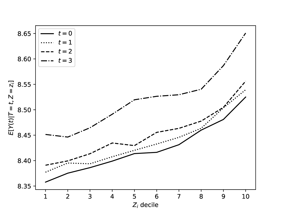
Figure 11: Estimated conditional moments of log-wages given ability and education level.

We first test whether cMIV is a reasonable assumption in our setup by implementing the test developed in Section 4.2. To that end, we use the parameters and kernel functions recommended by Chetverikov (2019) and focus on the theoretically most powerful procedure, the step-down approach. The estimated $p$-value of the test is $0.29$, see Table 1. We thus conclude that cMIV-p is a credible assumption provided that MIV holds.

$t$	$R^{st}_{t}$	$R^{crit}_{t;0.1}$	$p$-value	$n_{t}$
0	0.98	2.33	0.34	274295
1	-1.17	2.17	0.95	143299
2	-1.51	2.30	1.00	216336
3	1.86	2.38	0.08	30703

Table 1: Results of the monotonicity test, see Section 4.2. Second column gives the estimated Chetverikov (2019) test-statistic, third column contains the $\alpha=0.1$ critical values, corresponding to $\alpha_{t}=1-(1-0.1)^{1/4}\approx 0.026$ individual critical value. The last column gives a $p$-value against the individual null for each $t$. The overall $p$-value is $0.29$.

The data we study is rather noisy. One would expect a considerable measurement error in the construction of both treatment levels and the outcome variable. In line with that, the strongest form of cMIV is not sufficient to provide identification in the absence of further assumptions. While the resulting bounds are tighter than that under MIV, they remain uninformative.

To achieve identification, we supplement our assumptions with the MTR condition, which appears reasonable in our setting. The estimated bounds and confidence intervals are presented in Figure 12. While MIV and cMIV-w remain uninformative, both cMIV-p and cMIV-s yield positive lower bounds on the ATEs. Under cMIV-p, the effect of obtaining a university education is estimated to be at least $3.54\%$, and at least $5.5\%$ under cMIV-s. These findings align with previous evidence: causal estimates for the U.S. (Card (1993), Brand and Xie (2010), Angrist and Chen (2011)) suggest returns of at least $10\%$ for a four-year college degree. Recent evidence indicates that this figure may be substantially lower for Colombia Gomez (2022).

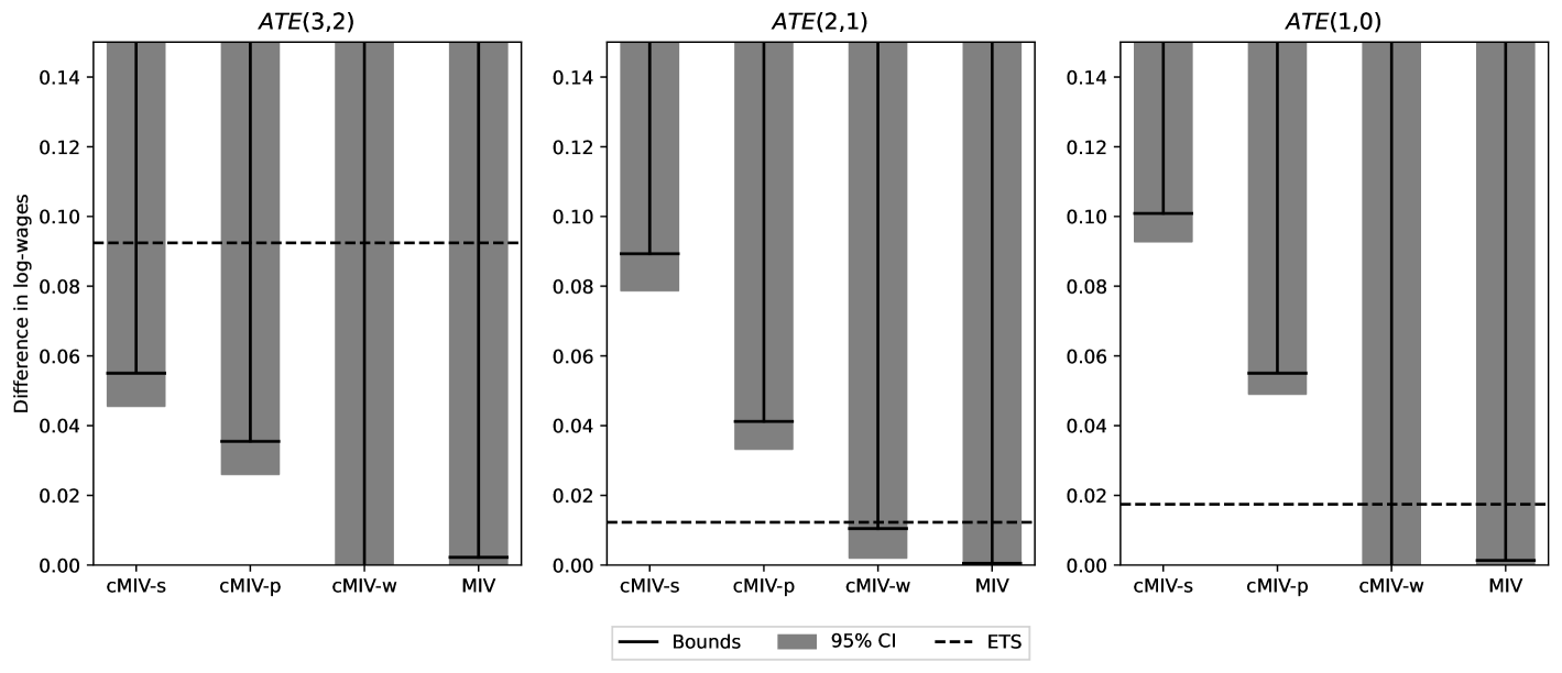
Figure 12: Estimation results for the monotonicity assumptions augmented with MTR. $5\%$ two-sided CI constructed according to Algorithm 1 using $2.5\%$ one-sided bounds. Parameters are selected according to Appendix H and E.2. The bounds’ point estimates are given by $\breve{B}$, while the exogenous treatment selection (ETS) estimates are the sample analogues of $ATE^{ETS}_{t,d}\equiv\mathbb{E}[Y|T=t]-\mathbb{E}[Y|T=d]$.

We also find significantly positive effects at other education stages, see Figure 12. Further results and details on the estimation procedure are available in Appendix J.

Part Online Appendices

Appendix A Consistency of penalty function estimators

A.1. Proof of Lemma 2.1.a

Proof.

Recall that for any sets $A,B$, we have $\inf A\cup B=\min\{\inf A,\inf B\}$. Fix any $(\theta,w)\in\mathbb{R}^{S}\times\mathbb{R}^{q}$ such that $\Theta_{I}(\theta)\subseteq\mathcal{X}$ and take $A\equiv L(\Theta_{I}(\theta);\theta,w)$, $B\equiv L(\mathcal{X}\cap\Theta_{I}(\theta)^{\prime};\theta,w)$. Note that $A\cup B=L(\mathcal{X};\theta,w)$. Substituting the definitions, it follows that

$$\tilde{B}(\theta;w)=\min\{\inf_{x\in\Theta_{I}(\theta)}p^{\prime}x, \inf_{x\in\mathcal{X}\cap\Theta_{I}(\theta)^{\prime}}p^{\prime}x+w^{\prime}(c-Mx)^{+}\}$$

$$=\min\{B(\theta), \inf_{xx\in\mathcal{X}\cap\Theta_{I}(\theta)^{\prime}}p^{\prime}x+w^{\prime}(c-Mx)^{+}\}\leq B(\theta),$$

which establishes (6).

For the second part, fix any pair $(\theta_{0},w)$ that satisfies Assumption A0. We write $\theta_{0}=(p^{\prime},\text{vec}(M)^{\prime},c^{\prime})^{\prime}$. Let $\lambda^{*}$ be the KKT vector from Assumption A1. The definition of KKT vector (see Section 28 in Rockafellar (1970)) requires that

$$B(\theta_{0})=\inf_{x\in\mathbb{R}^{d}}p^{\prime}x+\lambda^{*\prime}(c-Mx).$$ (32)

Note that, for any $x\in\mathbb{R}^{d}$,

$$B(\theta_{0})\leq p^{\prime}x+\lambda^{*\prime}(c-Mx)\leq p^{\prime}x+\lambda^{*\prime}(c-Mx)^{+}\leq p^{\prime}x+w^{\prime}(c-Mx)^{+},$$ (33)

where the first inequality follows from (32), the second inequality follows from $\lambda^{*}\geq 0$ and $(t)^{+}\geq t$ for any $t\in\mathbb{R}$, and the third inequality follows by Assumption A1. Taking infinum over $x\in\mathcal{X}$ on both sides of (33) and combining with (6) yields

$$\tilde{B}(\theta_{0};w)=B(\theta_{0})$$ (34)

We now wish to show that $\mathcal{A}(\theta_{0})=\tilde{\mathcal{A}}(\theta_{0};w)$. From (34), the fact that $L(x;\theta_{0},w)=p^{\prime}x$ for $x\in\Theta_{I}(\theta_{0})$ and $\mathcal{A}(\theta_{0})\subseteq\Theta_{I}(\theta_{0})$, it follows that:

$$\mathcal{A}(\theta_{0})\subseteq\tilde{\mathcal{A}}(\theta_{0};w)$$ (35)

To establish the other direction, we proceed by contradiction. Suppose $\exists x^{*}\in\tilde{\mathcal{A}}(\theta_{0};w)\cap\mathcal{A}(\theta_{0})^{\prime}$. Suppose $x^{*}\in\Theta_{I}(\theta_{0})$. Since $x^{*}\notin\mathcal{A}(\theta_{0})$, it must then be that $p^{\prime}x^{*}>B(\theta_{0})$, but $\tilde{B}(\theta_{0};w)=L(x^{*};\theta_{0},w)=p^{\prime}x^{*}$, which yields a contradiction with (34). So, $x^{*}\notin\Theta_{I}(\theta_{0})$. Consider

$$\tilde{B}(\theta_{0};w)=p^{\prime}x^{*}+w^{\prime}(c-Mx^{*})^{+}>p^{\prime}x^{*}+\lambda^{*\prime}(c-Mx^{*})^{+}\geq p^{\prime}x^{*}+\lambda^{*\prime}(c-Mx^{*})$$ (36)

where the first inequality follows from Assumption A1 and the fact that $x^{*}\notin\Theta_{I}(\theta_{0})\implies\exists j:c_{j}-M_{j}x^{*}>0$. Combining (36) with (32), one gets $\tilde{B}(\theta_{0};w)>B(\theta_{0})$, which yields a contradiction with (34). So, $\mathcal{A}(\theta_{0})\supseteq\tilde{\mathcal{A}}(\theta_{0};w)$. Combining with (35) establishes

$$\mathcal{A}(\theta_{0})=\tilde{\mathcal{A}}(\theta_{0};w).$$

This concludes the proof of the lemma. ∎

A.2. Proof of Theorem 2.1.a

Proof.

Fix the true $\theta_{0}=(p^{\prime},\text{vec}(M)^{\prime},c^{\prime})^{\prime}$. Recall that for any $g_{1},g_{2}\in\mathcal{C}(\mathcal{X})$, we can bound

$$|\inf_{\mathcal{X}}g_{1}-\inf_{\mathcal{X}}g_{2}|\leq\sup_{\mathcal{X}}|g_{1}-g_{2}|.$$ (37)

Clearly, $L(\cdot;\theta,w)\in\mathcal{C}(\mathcal{X})$ for any $(\theta,w)\in\mathbb{R}^{S}\times\mathbb{R}_{+}$. Using this, the bound (37) and the definition of $\tilde{B}(\cdot)$, one gets

$$|\tilde{B}(\hat{\theta}_{n};w_{n})-\tilde{B}(\theta_{0};w_{n})|\leq\sup_{x\in\mathcal{X}}|L(x;\hat{\theta}_{n},w_{n})-L(x;\theta_{0},w_{n})|$$ (38)

Using the definition of $L(\cdot)$, triangle and Cauchy-Schwarz inequalities, for every $x\in\mathcal{X}$

$$|L(x;\hat{\theta}_{n},w_{n})-L(x;\theta_{0},w_{n})|\leq||\hat{p}_{n}-p||\cdot||x||+w_{n}\sqrt{q}||(\hat{c}_{n}-\hat{M}_{n}x)^{+}-(c-Mx)^{+}||.$$ (39)

It is straightforward to observe that for any $v_{1},v_{2}\in\mathbb{R}^{q}$

$$||v^{+}_{1}-v^{+}_{2}||\leq||v_{1}-v_{2}||$$ (40)

Further, recall that for any $A\in\mathbb{R}^{q\times d}$ and $x\in\mathbb{R}^{d}$

$$||Ax||\leq||x||\sup_{||y||\leq 1}||Ay||=||x||\cdot||A||_{2},$$ (41)

where $||A||_{2}$ is the spectral norm of $A$. Also recall that if $||\cdot||_{F}$ is the Frobenius norm,

$$||A||_{2}\leq||A||_{F}=||\text{vec}(A)||.$$ (42)

Combining (40), (41), (42) and using triangle inequality, one gets

$$|L(x;\hat{\theta}_{n},w_{n})-L(x;\theta_{0},w_{n})|\leq||\hat{p}_{n}-p||\cdot||x||$$

$$+w_{n}\sqrt{q}\left(||\hat{c}_{n}-c||+||\text{vec}(\hat{M}_{n})-\text{vec}(M)||\cdot||x||\right),$$

where taking sup on both sides and using (38) yields

$$|\tilde{B}(\hat{\theta}_{n};w_{n})-\tilde{B}(\theta_{0};w_{n})|\leq||\hat{p}_{n}-p||\cdot||x||_{\infty}$$ (43)

$$+w_{n}\sqrt{q}\left(||\hat{c}_{n}-c||+||\text{vec}(\hat{M}_{n})-\text{vec}(M)||\cdot||x||_{\infty}\right)=O_{p}\left(\frac{w_{n}}{\sqrt{n}}\right),$$

where $||x||_{\infty}=\sup_{x\in\mathcal{X}}||x||<\infty$ by Assumption A0.ii, and the last equality follows from Assumption A0.iii.

Finally, since $\theta_{0}$ satisfies A0, there exists some $\lambda^{*}$ in $\Uplambda(\theta_{0})$ with $||\lambda^{*}||_{\infty}<\infty$. Let $E_{n}\equiv\{w_{n}>||\lambda^{*}||_{\infty}\}$. By Lemma 2.1.a, $E_{n}\subseteq\{\tilde{B}(\theta_{0};w_{n})=B(\theta_{0})\}$, so, for any deterministic $\{r_{n}\}_{n\in\mathbb{N}}$ and any $\varepsilon>0$,

$$\mathbb{P}\left[r_{n}|\tilde{B}(\hat{\theta}_{n};w_{n})-B(\theta_{0})|>\varepsilon\right]=$$ (44)

$$\mathbb{P}\left[r_{n}|\tilde{B}(\hat{\theta}_{n};w_{n})-\tilde{B}(\theta_{0};w_{n})|>\varepsilon,E_{n}\right]+\mathbb{P}\left[r_{n}|\tilde{B}(\hat{\theta}_{n};w_{n})-B(\theta_{0})|>\varepsilon,E_{n}^{\prime}\right]\leq$$

$$\mathbb{P}\left[r_{n}|\tilde{B}(\hat{\theta}_{n};w_{n})-\tilde{B}(\theta_{0};w_{n})|>\varepsilon\right]+\mathbb{P}[E^{\prime}_{n}]$$

By definition, $w_{n}\to\infty$ w.p.a.1 implies $\mathbb{P}[w_{n}>||\lambda^{*}||_{\infty}]\to 1$, so $\mathbb{P}[E^{\prime}_{n}]\to 0$. Combining this, (43) and (44), one obtains:

$$\tilde{B}(\hat{\theta}_{n};w_{n})-B(\theta_{0})=O_{p}\left(\frac{w_{n}}{\sqrt{n}}\right)$$

This concludes the proof of the Theorem.

∎

A.3. Proof of Theorem 2.1.b

Proof.

Fix $\theta=(p^{\prime},\text{vec}(M)^{\prime},c^{\prime})^{\prime}=\theta_{0}$. We proceed in six steps, first proving the following lemma: Consider $B\equiv\arg\min_{x\in A}f(x)$ and $c\equiv f(x^{*})$ for any $x^{*}\in B$, where $f(\cdot)$ is continuous and $A$ is a non-empty compact. Then, for any measurable random sequence $\{x_{n}\}\subseteq A$ such that $f(x_{n})\xrightarrow{p}c$, there exists a measurable random sequence $\{x^{*}_{n}\}\subseteq B$ such that $||x^{*}_{n}-x_{n}||\xrightarrow{p}0$.

Proof.

Under the assumptions of the Lemma, Berge’s maximum theorem implies that $B$ is a non-empty compact. Because the distance is continuous, the projection $x^{*}_{n}$ of $x_{n}$ onto $B$ is always well-defined for each $n$. If it is not unique, we select one of the values that yield the minimum distance. Measurability of at least one such selection is established by reference to Theorem 18.19 in Aliprantis and Border (2007). We then proceed by contradiction. Suppose that $\exists\varepsilon>0$:

$$\mathbb{P}[||x^{*}_{n}-x_{n}||>\varepsilon]\not\to 0$$ (45)

Then, there exists a $\delta>0$ and a subsequence $\{n_{k}\}^{\infty}_{k=1}$ such that, for all $k\in\mathbb{N}$:

$$\mathbb{P}[||x^{*}_{n_{k}}-x_{n_{k}}||>\varepsilon]>\delta$$ (46)

Consider the following problem:

$$\min_{x\in A,\leavevmode\nobreak\ d(x,B)\geq\varepsilon}f(x)$$ (47)

Notice that the constraint set is compact. It is also non-empty, as for any $k$ some of the realisations of $x_{n_{k}}$ are in it by (46). Therefore the minimum is attained at some $\tilde{x}$. Suppose that the minimum is equal to $f(\tilde{x})=\tilde{c}$. If $\tilde{c}=c$, it follows that $\tilde{x}\in B$, which is not possible as $d(\tilde{x},B)\geq\varepsilon$. Clearly, $\tilde{c}<c$ is also infeasible as the constraint set of that problem is smaller than that of the original one. Therefore, $\tilde{c}-c=K>0$. Then, note that for any $k\in\mathbb{N}$:

$$||x^{*}_{n_{k}}-x_{n_{k}}||>\varepsilon\implies f(x_{n_{k}})\geq f(\tilde{x})=c+K>c$$ (48)

So,

$$\mathbb{P}[f(x_{n_{k}})-f(x^{*})\geq K]\geq\mathbb{P}[||x^{*}_{n_{k}}-x_{n_{k}}||>\varepsilon]>\delta>0,$$ (49)

where the LHS goes to $0$ as $k\to\infty$, since $f(x_{n_{k}})\xrightarrow{p}f(x^{*})$ by assumption of the Lemma. This yields a contradiction. Therefore, $||x^{*}_{n}-x_{n}||\xrightarrow{p}0$. ∎

1. We first prove that $\exists$ $\{\delta_{n}\}\to 0^{+}$ such that $\mathcal{A}(\hat{\theta}_{n},w_{n})\subseteq\mathcal{A}(\theta_{0})^{\delta_{n}}$ w.p. $1$ asymptotically. For this purpose, recall that by Theorem 3 for any sequence $x_{n}\in\mathcal{A}(\hat{\theta}_{n},w_{n})$ for all $n$ and for any $x^{*}\in\mathcal{A}(\theta_{0})$, we have:

   $$p^{\prime}x_{n}+w_{n}\iota^{\prime}(\hat{c}_{n}-\hat{M}_{n}x_{n})^{+}-p^{\prime}x^{*}=o_{p}(1)$$ (50)

   Furthermore, since $w_{n}=o_{p}(\sqrt{n})$, we have:

   $$w_{n}||\hat{c}_{n}-\hat{M}_{n}x-c+Mx||_{\infty}=o_{p}(1)$$ (51)

   Because the argmin is contained in a compact, $\mathcal{A}(\hat{\theta}_{n},w_{n})\subseteq\mathcal{X}$, the first term in (50) is bounded in probability: $p^{\prime}x_{n}=O_{p}(1)$, thus, from (50), it also follows that $w_{n}\iota(\hat{c}_{n}-\hat{M}_{n}x_{n})^{+}=O_{p}(1)$. By triangle inequality and using with (51), we therefore conclude:

   $$w_{n}\iota^{\prime}(c-Mx_{n})^{+}=O_{p}(1)$$ (52)

   As $w_{n}\to\infty$, it further follows that:

   $$(c-Mx_{n})^{+}=o_{p}(1)$$ (53)

   We shall now consider $\tilde{x}_{n}$ - a projection of $x_{n}$ onto $\{x\in\mathbb{R}^{d}|Mx\geq c\}$. Note that it exists, because distance is a continuous function and the set is a non-empty compact. Note that $\eqref{conv_to_set}$ implies that, for some random $\kappa_{n}\geq 0$ for all $n$:

   $$c-Mx_{n}\leq\iota\kappa_{n}$$ (54)

   where $\kappa_{n}=o_{p}(1)$. We get:

   $$||x_{n}-\tilde{x}_{n}||=d(x_{n},\{x\in\mathbb{R}^{d}|Mx\geq c\})\leq$$ (55)

   $$\leq d_{H}(\{x\in\mathbb{R}^{d}|Mx\geq c-\kappa_{n}\},\{x\in\mathbb{R}^{d}|Mx\geq c\})\leq C\kappa_{n},$$ (56)

   where $C>0$ is some fixed constant. The first equality is by definition of projection, the second inequality follows from the definition of the Hausdorff distance and (54) as well as:

   $$d(x_{n},\{x\in\mathbb{R}^{d}|Mx\geq c\})\leq\underset{x\in\{x\in\mathbb{R}^{d}|Mx\geq c-\kappa_{n}\}}{\sup}d(x,\{x\in\mathbb{R}^{d}|Mx\geq c\}))$$ (57)

   The final inequality is implied by Lipschitz-continuity of polytopes in Hausdorff distance with respect to RHS expansions (see Li (1993)). Therefore:

   $$\tilde{x}_{n}-x_{n}\xrightarrow{p}0$$ (58)

   We now wish to show that $p^{\prime}x_{n}\xrightarrow{p}p^{\prime}x^{*}$, where $x^{*}$ is some value from $\mathcal{A}(\theta_{0})$. For arbitrary $\varepsilon>0$ note that:

   $$\mathbb{P}[|p^{\prime}x_{n}+w_{n}\iota^{\prime}(\hat{c}_{n}-\hat{M}_{n}x_{n})-p^{\prime}x^{*}|>\varepsilon]\geq$$ (59)

   $$\mathbb{P}[p^{\prime}x_{n}>p^{\prime}x^{*}+\varepsilon-w_{n}\iota^{\prime}(\hat{c}_{n}-\hat{M}_{n}x_{n})]\geq$$ (60)

   $$\mathbb{P}[p^{\prime}x_{n}>p^{\prime}x^{*}+\varepsilon]$$ (61)

   As the LHS goes to $0$ by (50), we have:

   $$\mathbb{P}[p^{\prime}x_{n}>p^{\prime}x^{*}+\varepsilon]\to 0$$ (62)

   To prove the other side, note that, as $\tilde{x}_{n}\in\Theta_{I}(\theta_{0})$, by definition of $x^{*}$, it must be that $p^{\prime}\tilde{x}_{n}\geq p^{\prime}x^{*}$. Therefore,

   $$\mathbb{P}[p^{\prime}x_{n}<p^{\prime}x^{*}-\varepsilon]\leq\mathbb{P}[p^{\prime}x_{n}<p^{\prime}\tilde{x}_{n}-\varepsilon]\to 0,$$ (63)

   where the RHS converges to $0$ by (58) and CMT. We thus conclude that $p^{\prime}x_{n}\xrightarrow{p}p^{\prime}x^{*}$ and, moreover, $p^{\prime}\tilde{x}_{n}\xrightarrow{p}p^{\prime}x^{*}$.

   Notice that by Lemma 2, for a fixed, large enough $w$ satisfying Assumption A1 Lemma A.3 applies, where one sets $f(x)=L(x;\theta_{0},w)$, $B=\mathcal{A}(\theta_{0})$ with $f(x^{*})=p^{\prime}x^{*}$ for any $x^{*}\in\mathcal{A}(\theta_{0})$. Thus, $\exists x^{*}_{n}\in\mathcal{A}(\theta_{0})$ such that $||x_{n}-x^{*}_{n}||\xrightarrow{p}0$. Therefore, $\exists\delta_{n}\to 0^{+}$ such that:

   $$\mathbb{P}[||x_{n}-x^{*}_{n}||<\delta_{n}]\to 1$$ (64)

   Recall that the sequence $x_{n}$ was arbitrarily selected from $\mathcal{A}(\hat{\theta}_{n},w_{n})$, and we can, for example, select a measurable $\{x_{n}\}^{\infty}_{n=1}$ (by Theorem 18.19 in Aliprantis and Border (2007)):

   $$x_{n}\in\underset{x\in\mathcal{A}(\hat{\theta}_{n},w_{n})}{\arg\max}d(x,\mathcal{A}(\theta_{0}))$$ (65)

   For such $x_{n}$, we get:

   $$||x_{n}-x^{*}_{n}||<\delta_{n}\implies d(x,\mathcal{A}(\theta_{0}))<\delta_{n}\leavevmode\nobreak\ \forall x\in\mathcal{A}(\hat{\theta}_{n},w_{n})$$ (66)

   So:

   $$\mathbb{P}[\mathcal{A}(\hat{\theta}_{n},w_{n})\subseteq\mathcal{A}(\theta_{0})^{\delta_{n}}]\geq\mathbb{P}[||x_{n}-x^{*}_{n}||<\delta_{n}]\to 1$$ (67)

   This establishes the existence of a deterministic $\delta_{n}\to 0^{+}$ such that $\mathcal{A}(\hat{\theta}_{n},w_{n})\subseteq\mathcal{A}(\theta_{0})^{\delta_{n}}$ w.p.a.1.

2. By (67) and using the representation found in Proposition F.2 we have that:

   $$\underset{x\in\mathcal{X}}{\inf}\leavevmode\nobreak\ L(x;\hat{\theta}_{n},w_{n})=\underset{x\in\mathcal{A}(\theta_{0})^{\delta_{n}}}{\inf}\leavevmode\nobreak\ L(x;\hat{\theta}_{n},w_{n})+o_{p}(1)$$ (68)

   $$=\underset{x\in\mathcal{A}(\theta_{0})^{\delta_{n}}}{\min}p^{\prime}x+w_{n}\underset{j\in[2^{q}]}{\max}\leavevmode\nobreak\ \left\{\sum_{i\in\Pi_{j}}(\hat{c}_{ni}-\hat{M}_{ni}^{\prime}x)\right\}+o_{p}(1),$$ (69)

   where $o_{p}(1)$ encompasses realizations at which $\mathcal{A}(\hat{\theta}_{n},w_{n})\notin\mathcal{A}(\theta_{0})^{\delta_{n}}$ or where $\hat{\theta}_{n}$ is not in a fixed open vicinity of $\theta_{0}$ that was argued to exist in Proposition F.2. Suppose that at $\theta_{0}$ the constraints that do not bind at any $x\in\mathcal{A}(\theta_{0})$ are given by $I\subseteq\{1,2,\dots,q\}$. By continuity, it follows that $\exists$ $\delta>0$ and $\varepsilon>0$ such that:

   $$c_{i}-M_{i}x<-\varepsilon,\forall i\in I$$ (70)

   for any $x\in\mathcal{A}(\theta_{0})^{\delta}$. From (67) it then also follows that:

   $$\underset{x\in\mathcal{X}}{\inf}\leavevmode\nobreak\ L(x;\hat{\theta}_{n},w_{n})=\underset{x\in\mathcal{A}(\theta_{0})^{\delta_{n}}}{\min}p^{\prime}x+w_{n}\underset{\Pi\in 2^{[q]\setminus I}}{\max}\leavevmode\nobreak\ \left\{\sum_{i\in\Pi_{j}}(\hat{c}_{ni}-\hat{M}_{ni}^{\prime}x)\right\}+o_{p}(1)$$ (71)

3. Consider the problem in the linear programming representation found in Proposition F.2, which it admits w.p.a. $1$:

   $$\inf_{x\in\mathcal{X}}L(x;\hat{\theta}_{n};w_{n})=\underset{t,x}{\min}\leavevmode\nobreak\ t\quad\text{s.t.: }\begin{cases}t\in[\underline{t};\overline{t}]\\ x\in\mathcal{X}\\ p^{\prime}x+\sum_{i\in\Pi_{j}}w_{n}(\hat{c}_{ni}-\hat{M}_{ni}^{\prime}x)\leq t,j\in[2^{q}]\end{cases}$$ (72)

   The Lagrangian reads as:

   $$\mathcal{L}=t+\sum_{\Pi\in 2^{[q]}}\lambda_{\Pi}\left(p^{\prime}x-t+w_{n}\sum_{j\in\Pi}\hat{c}_{nj}-\hat{M}_{nj}^{\prime}x\right),$$ (73)

   Where the constraints $x\in\mathcal{X}$ and $t\in[\underline{t};\overline{t}]$ are omitted, as they are not binding with probability $1$ as. This holds, as $\mathcal{A}(\theta_{0})\subseteq Int(\mathcal{X})$ and $B(\theta_{0})\in Int([\underline{t};\overline{t}])$ by assumption. Because $\mathcal{A}(\theta_{0})$ is compact, there further exists a $\overline{\delta}>0$: $\mathcal{A}(\theta_{0})^{\overline{\delta}}\subseteq Int(\mathcal{X})$ and as $\tilde{\mathcal{A}}(\hat{\theta}_{n};w_{n})\subseteq\mathcal{A}(\theta_{0})^{\delta_{n}}$ w.p.a. $1$ for some $\delta_{n}\to 0^{+}$, it follows that w.p.a.1 $\mathcal{A}(\hat{\theta}_{n};w_{n})\subseteq Int(\mathcal{X})$. Similar argument establishes that $t^{*}_{n}\in Int([\underline{t};\overline{t}])$ w.p.a.1. In what follows, we will simply call such optimal pairs interior.

   Differentiating with respect to $t$, one notes that:

   $$\sum_{\Pi}\lambda_{\Pi}=1$$ (74)

   Next, at any interior optimal $t,x$:

   $$t=p^{\prime}x+w_{n}\underset{\Pi}{\max}\sum_{j\in\Pi}(\hat{c}_{nj}-\hat{M}_{nj}^{\prime}x)$$ (75)

   To see that, note that by contradiction, if:

   $$t>p^{\prime}x+w_{n}\underset{\Pi}{\max}\sum_{j\in\Pi}(\hat{c}_{nj}-\hat{M}_{nj}^{\prime}x)$$ (76)

   Then, as we assumed that the pair $(t,x)$ is interior, there exists $\tilde{t}<t$ such that the pair $(\tilde{t},x)$ satisfies all the constraints. Therefore, $(t,x)$ is not optimal. The other direction of the inequality is infeasible, and so the equality must hold. Moreover, since $\Pi$ may be empty, we also have at any optimal $x$:

   $$t\geq p^{\prime}x$$ (77)

   Furthermore, the problem has a solution w.p.a.1, and therefore it has a vertex-solution, i.e. a solution that is pinned down by a matrix of binding constraints of full column-rank. Because w.p.a.1 any solution is interior, any such matrix w.p.a.1 does not feature constraints $x\in\mathcal{X},t\in[\underline{t},\overline{t}]$. The only constraints that can be satisfied at such vertex-solution with an equality are of the following type:

   $$p^{\prime}x-t=w_{n}\sum_{j\in\Pi_{k}}\hat{c}_{nj}-\hat{M}_{nj}^{\prime}x,\leavevmode\nobreak\ k\in\tilde{J}$$ (78)

   for some $\tilde{J}\subseteq 2^{[q]}:|\tilde{J}|\geq d+1$, where the latter inequality holds by definition of a vertex of a linear program. One can write the complete set of the binding constraints (78) as:

   $$\hat{R}_{\tilde{J}n}\begin{pmatrix}t\\ x\end{pmatrix}=\hat{r}_{n}^{\tilde{J}},$$ (79)

   where the $|\tilde{J}|\times(d+1)$ matrix $\hat{R}_{\tilde{J}n}$ is of full column rank and the system yields a unique solution $t^{*}_{n},x^{*}_{n}$.

4. Denote the set of all vertices $(t^{*},x^{*})$ that satisfy (78) with $|\tilde{J}|\geq d+1$ and a full-column-rank $\hat{R}_{\tilde{J}n}$ at a given $\hat{\theta}_{n}$ by $\mathcal{V}^{*}(\hat{\theta}_{n})$. From the previous arguments it follows that $\mathcal{V}^{*}(\cdot)$ is non-empty w.p.a.1 and finite, because any finite-dimensional polytope has finitely many vertices and therefore the corresponding LP has finitely many optimal vertices. We will write $\mathcal{V}_{x}^{*}(\hat{\theta}_{n})$ for the projection of that set on the $x$-coordinates. For any vertex-solution $(t^{*},x^{*})\in\mathcal{V}^{*}(\hat{\theta}_{n})$, suppose constraints $V^{*}\subseteq\{1,\dots q\}$ are violated at it, meaning that:

   $$V^{*}(\hat{\theta}_{n},x^{*})\equiv\{j\in[q]|\hat{c}_{nj}-\hat{M}_{nj}^{\prime}x^{*}>0\}$$ (80)

   For brevity, we will write $V^{*}_{n}\equiv V^{*}(\hat{\theta}_{n},x_{n}^{*})$ where $t^{*}_{n},x_{n}^{*}\in\mathcal{V}^{*}(\hat{\theta}_{n})$ is some (measurable) sequence of optimal vertices. Note that:

   $$t^{*}_{n}=p^{\prime}x^{*}_{n}+w_{n}\underset{\Pi}{\max}\sum_{j\in\Pi}(\hat{c}_{nj}-\hat{M}_{nj}^{\prime}x^{*}_{n})=p^{\prime}x^{*}_{n}+w_{n}\sum_{j\in V_{n}^{*}}(\hat{c}_{nj}-\hat{M}_{nj}^{\prime}x^{*}_{n})$$ (81)

   Consider (78) and suppose $\tilde{J}_{n}=\tilde{J}(t^{*}_{n},x^{*}_{n})$ with $|\tilde{J}_{n}|\geq d+1$ is the set of the corresponding subsets, i.e.:

   $$t^{*}_{n}=p^{\prime}x^{*}_{n}+w_{n}\sum_{j\in\Pi_{i}}(\hat{c}_{nj}-\hat{M}_{nj}^{\prime}x^{*}_{n})\leavevmode\nobreak\ \forall i\in[k]$$ (82)

   It must be that $V_{n}^{*}\subseteq\Pi_{i}$ $\forall i\in\tilde{J}_{n}$, because $j\notin V_{n}^{*}\implies(\hat{c}_{nj}-\hat{M}_{nj}^{\prime}x^{*}_{n})\leq 0$, and so we have:

   $$\sum_{j\in V_{n}^{*}}(\hat{c}_{nj}-\hat{M}_{nj}^{\prime}x^{*}_{n})=\sum_{j\in\Pi_{i}}(\hat{c}_{nj}-\hat{M}_{nj}^{\prime}x^{*}_{n})\leq\sum_{j\in\Pi_{i}\cap V_{n}^{*}}(\hat{c}_{nj}-\hat{M}_{nj}^{\prime}x^{*}_{n}),$$ (83)

   where the first equality follows from (82) and (81). We now proceed by contradiction. Suppose that $\exists j:j\in V_{n}^{*}\cap\Pi_{i}^{\prime}$ (where the complement is taken with respect to $[q]$), then:

   $$\sum_{j\in\Pi_{i}\cap V_{n}^{*}}(\hat{c}_{nj}-\hat{M}_{nj}^{\prime}x^{*}_{n})<\sum_{j\in\Pi_{i}\cap V_{n}^{*}}(\hat{c}_{nj}-\hat{M}_{nj}^{\prime}x^{*}_{n})+\sum_{j\in\Pi^{\prime}_{i}\cap V_{n}^{*}}(\hat{c}_{nj}-\hat{M}_{nj}^{\prime}x^{*}_{n})=$$

   $$=\sum_{j\in V_{n}^{*}}(\hat{c}_{nj}-\hat{M}_{nj}^{\prime}x^{*}_{n}),$$

   which yields a contradiction with (83), so there can be no such $j$. In light of (83) it then also follows that $\forall i\in\tilde{J}_{n}$ and $\forall j\in\Pi_{i}\cap V_{n}^{*\prime}$ it must be that:

   $$\hat{c}_{nj}-\hat{M}_{nj}^{\prime}x^{*}_{n}=0\leavevmode\nobreak\ \forall j\in\Pi_{k}\setminus V_{n}^{*}$$ (84)

   Therefore, the complete system described by equation (82), is equivalent to:

   $$\begin{cases}&\hat{c}_{nj}-\hat{M}_{nj}^{\prime}x^{*}_{n}=0\leavevmode\nobreak\ \forall i\in\tilde{J}_{n}:\Pi_{i}\neq V_{n}^{*},\leavevmode\nobreak\ \forall\leavevmode\nobreak\ j\in\Pi_{i}\setminus V_{n}^{*}\\ &t^{*}_{n}=p^{\prime}x^{*}_{n}+w_{n}\sum_{j\in V^{*}_{n}}\hat{c}_{nj}-\hat{M}^{\prime}_{nj}x^{*}_{n}\end{cases}$$ (85)

   From the representation (79), we know that the matrix corresponding to system (85) must be of full column rank, $d+1$. Dropping the equation defining $t_{n}^{*}$, it implies that there exists at least $d$ linearly independent equations of form:

   $$\hat{c}_{nj}-\hat{M}_{nj}^{\prime}x^{*}_{n}=0$$

   We denote the set of all binding constraints by $\Pi^{*}(\hat{\theta}_{n},x^{*}_{n})\equiv\{j\in[q]|\hat{c}_{nj}-\hat{M}_{nj}^{\prime}x^{*}_{n}=0\}$, which we shall occasionally write as $\Pi_{n}^{*}$ for brevity. We thus have:

   $$|\Pi^{*}_{n}|\geq d,\quad\text{rk}(\hat{M}_{\Pi^{*}_{n}})=d$$ (86)

5. Consider two collections of sets:

   $$\mathcal{E}\equiv\{A\subseteq 2^{[q]}:M_{A}x\neq c_{A}\leavevmode\nobreak\ \forall x\in\mathcal{A}(\theta_{0})\}$$ (87)

   $$\mathcal{F}\equiv\{A\subseteq 2^{[q]}:p\notin\mathcal{R}(M^{\prime}_{A})\}$$ (88)

   We shall now consider two events $E_{n}$ and $F_{n}$:

   $$E_{n}\equiv\{\Pi^{*}_{n}\in\mathcal{E}\},\quad F_{n}\equiv\{\Pi^{*}_{n}\in\mathcal{F}\}$$ (89)

   We wish to show that $\mathbb{P}[E_{n}]\to 0$ and $\mathbb{P}[F_{n}]\to 0$ and therefore $\mathbb{P}[E^{\prime}_{n}\cap F^{\prime}_{n}]\to 1$.

   1. Let us consider $E_{n}$ first. Since $\mathcal{A}(\theta_{0})$ is compact, for a fixed set $A\in\mathcal{E}$, the condition $M_{A}x\neq c_{A}\leavevmode\nobreak\ \leavevmode\nobreak\ \forall x\in\mathcal{A}(\theta_{0})$ implies that there exists $\varepsilon(A)>0$:

      $$\inf_{x\in\mathcal{A}(\theta_{0})}||M_{A}x-c_{A}||>\varepsilon(A)$$ (91)

      Because $E$ is a finite collection of sets, we can pick $\varepsilon=\min_{A\in E}\varepsilon(A)$, so that:

      $$\min_{A\in\mathcal{E}}\inf_{x\in\mathcal{A}(\theta_{0})}||M_{A}x-c_{A}||>\varepsilon$$ (92)

      By continuity of the objective function in $x$, there further $\exists\kappa>0$, such that:

      $$\min_{A\in\mathcal{E}}\inf_{x\in\mathcal{A}^{\kappa}(\theta_{0})}||M_{A}x-c_{A}||>\frac{\varepsilon}{2}$$ (93)

      We now consider:

      $$\mathbb{P}[E_{n}]\leq\mathbb{P}\left[||\hat{M}_{\Pi^{*}_{n}}x^{*}_{n}-\hat{c}_{\Pi^{*}_{n}}||=0,\inf_{x\in\mathcal{A}^{\kappa}(\theta_{0})}||M_{\Pi^{*}_{n}}x-c_{\Pi^{*}_{n}}||>\frac{\varepsilon}{2}\right]$$ (94)

      Observe that for any non-empty $A\subseteq[q]$, by Cauchy-Schwartz and triangle inequalities:

      $$||(\hat{M}_{nA}x^{*}_{n}-\hat{c}_{nA})||=$$

      $$\left|\left|(M_{A}x^{*}_{n}-c_{A})-\left((\hat{c}_{nA}-c_{A})+(M_{A}-\hat{M}_{nA})x^{*}_{n}\right)\right|\right|\geq$$

      $$\left|\left|M_{A}x^{*}_{n}-c_{A}\right|\right|-\left|\left|\hat{M}_{nA}-M_{A}\right|\right|||x||_{\infty}-\left|\left|\hat{c}_{nA}-c_{A}\right|\right|$$

      We can thus further rewrite:

      $$\mathbb{P}\left[||\hat{M}_{\Pi^{*}_{n}}x^{*}_{n}-\hat{c}_{\Pi^{*}_{n}}||\leq 0,\inf_{x\in\mathcal{A}^{\kappa}(\theta_{0})}||M_{\Pi^{*}_{n}}x-c_{\Pi^{*}_{n}}||>\frac{\varepsilon}{2}\right]\leq$$

      $$\mathbb{P}\left[\left|\left|M_{\Pi^{*}_{n}}x^{*}_{n}-c_{\Pi^{*}_{n}}\right|\right|\leq\eta_{n},\inf_{x\in\mathcal{A}^{\kappa}(\theta_{0})}||M_{\Pi^{*}_{n}}x-c_{\Pi^{*}_{n}}||>\frac{\varepsilon}{2}\right],$$

      where $\eta_{n}\equiv\left|\left|\hat{M}_{\Pi^{*}_{n}}-M_{\Pi^{*}_{n}}\right|\right|||x||_{\infty}+\left|\left|\hat{c}_{\Pi^{*}_{n}}-c_{\Pi^{*}_{n}}\right|\right|=o_{p}(1)$. Finally, using $\mathbb{P}[A\cap B^{\prime}]+\mathbb{P}[A\cap B]=\mathbb{P}[A]$:

      $$\mathbb{P}\left[\left|\left|M_{\Pi^{*}_{n}}x^{*}_{n}-c_{\Pi^{*}_{n}}\right|\right|\leq\eta_{n},\inf_{x\in\mathcal{A}^{\kappa}(\theta_{0})}||M_{\Pi^{*}_{n}}x-c_{\Pi^{*}_{n}}||>\frac{\varepsilon}{2}\right]=$$

      $$\mathbb{P}\left[\left|\left|M_{\Pi^{*}_{n}}x^{*}_{n}-c_{\Pi^{*}_{n}}\right|\right|\leq\eta_{n},\inf_{x\in\mathcal{A}^{\kappa}(\theta_{0})}||M_{\Pi^{*}_{n}}x-c_{\Pi^{*}_{n}}||>\frac{\varepsilon}{2},x_{n}^{*}\in\mathcal{A}^{\kappa}(\theta_{0})\right]+$$

      $$+\mathbb{P}\left[\left|\left|M_{\Pi^{*}_{n}}x^{*}_{n}-c_{\Pi^{*}_{n}}\right|\right|\leq\eta_{n},\inf_{x\in\mathcal{A}^{\kappa}(\theta_{0})}||M_{\Pi^{*}_{n}}x-c_{\Pi^{*}_{n}}||>\frac{\varepsilon}{2},x_{n}^{*}\notin\mathcal{A}^{\kappa}(\theta_{0})\right],$$

      where the second term is $o(1)$ by Step 1 of the proof. Finally, we note that $x^{*}_{n}\in\mathcal{A}^{\kappa}(\theta_{0})\implies\left|\left|M_{\Pi^{*}_{n}}x^{*}_{n}-c_{\Pi^{*}_{n}}\right|\right|>\varepsilon/2$, which, combined with $\left|\left|M_{\Pi^{*}_{n}}x^{*}_{n}-c_{\Pi^{*}_{n}}\right|\right|\leq\eta_{n}$, further implies that $\eta_{n}>\varepsilon/2>0$, so that:

      $$\mathbb{P}\left[\left|\left|M_{\Pi^{*}_{n}}x^{*}_{n}-c_{\Pi^{*}_{n}}\right|\right|\leq\eta_{n},\inf_{x\in\mathcal{A}^{\kappa}(\theta_{0})}||M_{\Pi^{*}_{n}}x-c_{\Pi^{*}_{n}}||>\frac{\varepsilon}{2},x_{n}^{*}\in\mathcal{A}^{\kappa}(\theta_{0})\right]\leq$$

      $$\mathbb{P}\left[\frac{\varepsilon}{2}\leq\eta_{n}\right]=o(1)$$

      This concludes the proof.

   2. We now consider $F_{n}$. To do so, it is convenient to observe that the penalty function estimator and problem (72) are equivalent to yet another LP:

      $$B(\hat{\theta}_{n})+o_{p}(1/\sqrt{n})=\underset{x,a}{\min\leavevmode\nobreak\ }p^{\prime}x+w_{n}\iota^{\prime}a\quad\text{s.t.}:\begin{cases}a\geq 0\\ a\geq\hat{c}_{n}-\hat{M}_{n}x\end{cases}$$ (95)

      Note that we drop the constraints corresponding to $x\in\mathcal{X}$ in (95), and $o_{p}(1/\sqrt{n})$ accommodates the potential non-existence of the interior solution. Write Lagrangian:

      $$\mathcal{L}=p^{\prime}x+w_{n}\iota^{\prime}a+\mu^{\prime}(\hat{c}_{n}-\hat{M}_{n}x-a)-\omega^{\prime}a$$

      The KKT conditions at an interior optimum are:

      $$p=\hat{M}_{n}^{\prime}\mu$$ (96)

      $$w_{n}=\omega+\mu$$ (97)

      $$\omega^{\prime}a=0$$ (98)

      $$\mu^{\prime}(\hat{c}_{n}-\hat{M}_{n}x-a)=0$$ (99)

      $$a\geq\hat{c}_{n}-\hat{M}_{n}x$$ (100)

      $$a\geq 0,\omega\geq 0,\mu\geq 0$$ (101)

      Analyzing the above system, one observes that if at $x^{*}_{n}\in\mathcal{V}^{*}_{x}(\theta_{n})$ a constraint is violated, $j\in V_{n}^{*}$, then $a_{j}>0$, and so $\omega_{j}=0$, which implies $\mu_{j}=w_{n}$. If $\hat{M}_{nj}x_{n}^{*}-\hat{c}_{nj}>0$, then $\hat{c}_{nj}-\hat{M}_{nj}x_{n}^{*}-a_{j}<0$, and so $\mu_{j}=0$. Finally, if $j\in\Pi_{n}^{*}$, then $\mu_{j}\in[0;w_{n}]$. Therefore, (96) rewrites as:

      $$p=w_{n}\sum_{j\in V_{n}^{*}}\hat{M}_{nj}^{\prime}+\sum_{j\in\Pi_{n}^{*}}\hat{M}_{nj}^{\prime}\mu_{j}$$ (102)

      Since $\mu_{j}\leq w_{n}$ and as $\hat{M}_{n}-M=O_{p}(1/\sqrt{n})$, we have:

      $$p=w_{n}\sum_{j\in V_{n}^{*}}M_{j}^{\prime}+\sum_{j\in\Pi_{n}^{*}}M_{j}^{\prime}\mu_{j}+O_{p}(\frac{w_{n}}{\sqrt{n}})$$ (103)

      Consider a projection $P_{\Pi_{n}^{*}}$ from $\mathbb{R}^{d}$ onto $\mathcal{R}(M^{\prime}_{\Pi_{n}^{*}})$. For example, one can construct it as $M^{\prime}_{\Pi_{n}^{*}}(M^{\prime}_{\Pi_{n}^{*}})^{\dagger}$, where $\dagger$ denotes a Moore-Penrose pseudoinverse. We can write:

      $$p-O_{p}(\frac{w_{n}}{\sqrt{n}})=w_{n}(I-P_{\Pi_{n}^{*}})\sum_{j\in V^{*}}M_{j}^{\prime}+\underbrace{w_{n}P_{\Pi_{n}^{*}}\sum_{j\in V^{*}}M_{j}^{\prime}+\sum_{j\in\Pi_{n}^{*}}M_{j}^{\prime}\mu_{j}}_{T_{n}\in\mathcal{R}(M^{\prime}_{\Pi_{n}^{*}})}$$ (104)

      Notice that, if $\sum_{j\in V^{*}}M_{j}^{\prime}\notin\mathcal{R}(M^{\prime}_{\Pi^{*}})$, then the RHS of (104) has unbounded norm:

      $$\left|\left|w_{n}(I-P_{\Pi_{n}^{*}})\sum_{j\in V_{n}^{*}}M_{j}^{\prime}+T_{n}\right|\right|^{2}=$$ (105)

      $$=w^{2}_{n}||(I-P_{\Pi_{n}^{*}})\sum_{j\in V_{n}^{*}}M_{j}^{\prime}||^{2}+||T_{n}||^{2}$$

      Since the square norm of the LHS of (104) is bounded from above by $||p||^{2}+O_{p}(\frac{w^{2}_{n}}{n})=||p||^{2}+o_{p}(1)$, (105) will contradict the equality in (104) w.p.a.1. Suppose, alternatively, that $\exists v:\sum_{j\in V_{n}^{*}}M_{j}^{\prime}=M^{\prime}_{\Pi_{n}^{*}}v$. Equation (104) rewrites:

      $$p-O_{p}(\frac{w_{n}}{\sqrt{n}})=M^{\prime}_{\Pi_{n}^{*}}(\mu_{\Pi_{n}^{*}}+w_{n}v),$$

      which implies, for example, that:

      $$(I-P_{\Pi_{n}^{*}})p+P_{\Pi_{n}^{*}}p-M^{\prime}_{\Pi_{n}^{*}}(\mu_{\Pi_{n}^{*}}+w_{n}v)=O_{p}(\frac{w_{n}}{\sqrt{n}})$$ (106)

      The norm of the LHS of (106) must go to $0$, however, if $p\notin\mathcal{R}(M^{\prime}_{\Pi_{n}^{*}})$, we have, by orthogonality:

      $$\left|\left|(I-P_{\Pi_{n}^{*}})p\right|\right|^{2}+\left|\left|P_{\Pi_{n}^{*}}p-M^{\prime}_{\Pi_{n}^{*}}(\mu_{\Pi_{n}^{*}}+w_{n}v)\right|\right|^{2}\geq\left|\left|(I-P_{\Pi_{n}^{*}})p\right|\right|^{2}>0,$$

      which will also yield a contradiction w.p.a.1. To complete the proof, one applies the same probabilistic arguments as used in step 5.a above, which we omit here. Thus, $\mathbb{P}[F_{n}]\to 0$.

6. We define the correct set of vertices, $\mathcal{G}$, as follows:

   $$\mathcal{G}\equiv\{A\subseteq[q]:\exists x\in\mathcal{A}(\theta_{0})\text{ s.t. }M_{A}x=c_{A},\leavevmode\nobreak\ p\in\mathcal{R}(M^{\prime}_{A})\}$$

   In line with previous notation, let $G_{n}\equiv\{\Pi^{*}_{n}\in\mathcal{G}\}$. The results of point 5 imply that $\mathbb{P}[E_{n}^{\prime}\cap F_{n}^{\prime}]=\mathbb{P}[G_{n}]\to 1$.

   Consider any $A\in\mathcal{G}$. Suppose $p=M_{A}^{\prime}v$ for some $v\in\mathbb{R}^{|A|}$. Further, fix any $x\in\mathcal{A}(\theta_{0}):M_{A}x=c_{A}$, then:

   $$B(\theta_{0})=p^{\prime}x=v^{\prime}M_{A}x=v^{\prime}c_{A}$$ (107)

   The conclusion then follows from the following chain of equalities:

   $$G_{n} \implies p^{\prime}x^{*}_{n}-B(\theta_{0})=v^{\prime}M_{\Pi^{*}_{n}}x^{*}_{n}-v^{\prime}c_{\Pi^{*}_{n}}=$$ (108)

   $$=v^{\prime}\hat{M}_{\Pi^{*}_{n}}x^{*}_{n}-v^{\prime}c_{\Pi^{*}_{n}}+v^{\prime}(M_{\Pi^{*}_{n}}-\hat{M}_{\Pi^{*}_{n}})x^{*}_{n}=$$ (109)

   $$=v^{\prime}(\hat{c}_{\Pi^{*}_{n}}-c_{\Pi^{*}_{n}})+v^{\prime}(M_{\Pi^{*}_{n}}-\hat{M}_{\Pi^{*}_{n}})x^{*}_{n}$$ (110)

   Finally, from (110), applying the triangle and Cauchy-Shwartz inequalities as well as noting that over the event $G_{n}$ one has $\Pi^{*}_{n}\in\mathcal{G}$ by definition, it follows that:

   $$G_{n}\implies|p^{\prime}x^{*}_{n}-B(\theta_{0})|\leq\varpi_{n}\equiv$$

   $$\max_{A\in\mathcal{G}}\left\{\left(||\hat{c}_{A}-c_{A}||+||x||_{\infty}||M_{A}-\hat{M}_{A}||\right)\cdot\min_{v\in\mathbb{R}^{|A|}:\leavevmode\nobreak\ M_{A}^{\prime}v=p}||v||\right\}$$

   One concludes by noting that the RHS is clearly $O_{p}(1/\sqrt{n})$, as $\mathcal{G}$ is finite and $\hat{\theta}_{n}-\theta_{0}=O_{p}(1/\sqrt{n})$ by assumption. Formally, for any $\varepsilon>0$:

   $$\mathbb{P}[r_{n}|p^{\prime}x^{*}_{n}-B(\theta_{0})|>\varepsilon]=\mathbb{P}[r_{n}|p^{\prime}x^{*}_{n}-B(\theta_{0})|>\varepsilon,G_{n}]+o(1)\leq$$ (111)

   $$\mathbb{P}[r_{n}\varpi_{n}>\varepsilon,G_{n}]+o(1)\leq\mathbb{P}[r_{n}\varpi_{n}>\varepsilon]+o(1)$$ (112)

   and $r_{n}\varpi_{n}=O_{p}(\frac{r_{n}}{\sqrt{n}})$ for any $r_{n}\to\infty$, where we used the fact that $\mathbb{P}[G^{\prime}_{n}\cap O_{n}]\leq\mathbb{P}[G^{\prime}_{n}]=o(1)$ for any measurable $O_{n}$. Recalling that the choice of $x^{*}_{n}\in\mathcal{V}^{*}_{x}(\hat{\theta}_{n})$ was arbitrary and that neither $\varpi_{n}$, nor the $o(1)$ depend on $x^{*}_{n}$, one gets:

   $$\sup_{x\in\mathcal{V}^{*}_{x}(\hat{\theta}_{n})}|p^{\prime}x-B(\theta_{0})|=O_{p}(1/\sqrt{n})$$ (113)

   But because any $x\in\mathcal{A}(\hat{\theta}_{n};w_{n})$ can be represented as a convex combination of vertices, $\{x_{j}\}^{K}_{j=1}\subseteq\mathcal{V}^{*}_{x}(\hat{\theta}_{n})$, as: $x=\sum_{j}\omega_{j}x_{j}$, where $\omega_{j}\in[0;1]$ and $\sum_{j}\omega_{j}=1$. Using that, applying the triangle inequality and taking maximum, one gets, for any $x\in\tilde{\mathcal{A}}(\hat{\theta}_{n};w_{n})$:

   $$|p^{\prime}x-B(\theta_{0})|=\left|\sum_{j}\omega_{j}(p^{\prime}x_{j}-B(\theta_{0})\right|\leq$$

   $$\max_{j}|p^{\prime}x_{j}-B(\theta_{0})|\leq\sup_{x\in\mathcal{V}^{*}_{x}(\hat{\theta}_{n})}|p^{\prime}x-B(\theta_{0})|=O_{p}\left(1/\sqrt{n}\right)$$

   taking supremum on the left hand side establishes the claim of the theorem.

∎

Appendix B Inference on the debiased estimator

B.1. Proof of Theorem 2.2.a

Proof.

For $x\in\mathbb{R}^{qd}$, define the inverse-vectorization operator as

$$\text{vec}_{q\times d}^{-1}(x)\equiv\left(\text{vec}(I_{d})^{\prime}\otimes I_{q}\right)(I_{d}\otimes x).$$

Further, define selector matrices $C_{c}$ and $C_{M}$ that select the $c$ and $M$ components of $\theta$ respectively:

$$C_{c}\theta=c,\quad C_{M}\theta=\text{vec}(M).$$

Moreover, for a subset of rows $A\subseteq\{1,2,\dots,q\}$, define the row-selector $C(A)$ as

$$C(A)M=M_{A},\quad C(A)c=c_{A}.$$

We first work on $\mathcal{D}^{(1)}_{n}$. From Step 5.b in the proof of Theorem 2.1.b, it follows that solving the penalized problem is w.p.a.1 equivalent to solving a relaxed LP, i.e., w.p.a.1,

$$\tilde{\mathcal{A}}(\hat{\theta}_{1};w_{n_{1}})=\min_{x\in\mathbb{R}^{d},a\in\mathbb{R}^{q}}p^{\prime}x+w_{n_{1}}\iota^{\prime}a,\quad\text{s.t.: }a\geq\hat{c}^{(1)}-\hat{M}^{(1)}x,\leavevmode\nobreak\ a\geq 0.$$ (114)

Denote the set of vertex-solutions of (114) by $\hat{\mathcal{V}}_{x}$ and consider

$$\hat{x}\in\arg\min_{x\in\hat{\mathcal{V}}_{x}}\leavevmode\nobreak\ p^{\prime}x,\quad\hat{A}=J(\hat{x};\hat{\theta}^{(1)}).$$

From Step 6 of the proof of Theorem 2.1.b it follows that $\hat{A}\in\mathbb{A}$ w.p.a.1.

For a nonempty $A\in 2^{[q]}$ and any $\tilde{M}\in\mathbb{R}^{q\times d}$, define

$$\mathbb{S}(A,\tilde{M})\equiv\arg\underset{v\in\mathbb{R}^{|A|}:||v||\leq\overline{v}}{\min}||p-\tilde{M}_{A}^{\prime}v||^{2}$$

The optimization problem above is continuous in $\tilde{M}$, the constraint correspondence is constant and compact. Hence, for any nonempty $A\in 2^{[q]}$, by Berge’s Maximum Theorem, $\mathbb{S}(A,\cdot)$ is compact, nonempty, and upper-hemicontinuous (see Theorem 17.31 in Aliprantis and Border (2007)).

Because $\hat{M}^{(1)}\xrightarrow{p}\hat{M}^{(1)}$, for any nonempty $A\in 2^{[q]}$ it follows by the usual M-estimation argument, there exists a deterministic $s_{n}(A)\downarrow 0$, such that

$$\mathbb{S}(A,\hat{M}^{(1)})\subseteq\mathbb{S}(A,M)^{s_{n}(A)},\quad\text{w.p.a.1},$$ (115)

so that also

$$\mathbb{S}(\hat{A},\hat{M}^{(1)})\subseteq\mathbb{S}(\hat{A},M)^{s_{n}(\hat{A})}\text{ w.p.a.1}$$ (116)

Observing that the objective function is convex, $\mathbb{S}(A,\tilde{M})$ is also convex-valued for any nonempty $A\in 2^{[q]}$ and $\tilde{M}\in\mathbb{R}^{q\times d}$.

Define some measurable $\check{v}\in\mathbb{S}(\hat{A},\hat{M}^{(1)})$ and denote its projection onto $\mathbb{S}(\hat{A},M)$ by $\tilde{v}_{n}$. Both $\check{v}$ is a random sequence, but we suppress the dependence on $n$ for simplicity. $\tilde{v}_{n}$ is well-defined by the Hilbert Projection Theorem. $\check{v}$ is well-defined, and $\tilde{v}_{n}$ is measurable by Theorem 18.19 in Aliprantis and Border (2007). From (116) it follows that

$$||\check{v}-\tilde{v}_{n}||=o_{p}(1)$$ (117)

By definition, $A\in\mathbb{A}$ implies that $\exists v^{*}\in\mathcal{S}_{A}$ such that $||v^{*}||\leq\underset{\tilde{A}\in\mathbb{A}}{\max}\underset{v\in\mathcal{S}_{\tilde{A}}}{\min}||v||\leq\overline{v}$, where the last inequality is by Assumption B3. This implies that, for any $A\in\mathbb{A}$,

$$\underset{v\in\mathbb{R}^{|A^{*}|}:||v||\leq\overline{v}}{\inf}||p-M_{A^{*}}^{\prime}v||^{2}=\underset{v\in\mathbb{R}^{|A^{*}|}:||v||\leq\overline{v}}{\min}||p-M_{A^{*}}^{\prime}v||^{2}=0.$$ (118)

By (118), we have $\mathbb{S}(A,M)\subseteq\mathcal{S}_{A}$ if $A\in\mathbb{A}$. Therefore, $\tilde{v}_{n}\in\mathcal{S}_{\hat{A}}$ w.p.a.1.

The following Lemma justifies our construction: Suppose $\hat{A}\in\mathbb{A}$. Then,

$$\tilde{v}_{n}^{\prime}c_{\hat{A}}=B(\theta_{0}),$$ (119)

$$\tilde{v}_{n}^{\prime}M_{\hat{A}}\hat{x}=p^{\prime}\hat{x}.$$ (120)

Proof.

If $\hat{A}\in\mathbb{A}$, condition (8) holds for some $x\in\mathcal{A}(\theta_{0})$ such that $M_{\hat{A}}x=c_{\hat{A}}$. Since such $x$ is a minimizer, it follows that $p^{\prime}x=B(\theta_{0})$. As $\tilde{v}_{n}\in\mathcal{S}_{\hat{A}}$, we have $p=M_{\hat{A}}^{\prime}\tilde{v}_{n}$. Taking transpose and multiplying by $\hat{x}$ yields (120). To show (119), write:

$$p^{\prime}x=\tilde{v}_{n}^{\prime}M_{\hat{A}}x=\tilde{v}_{n}^{\prime}c_{\hat{A}}$$

This concludes the proof of the Lemma. ∎

To avoid dealing with changing dimension, we let $\hat{v}\in\mathbb{R}^{q}$ be such that $\hat{v}_{\hat{A}}=\check{v}$ and $\hat{v}_{j}=0$ if $j\notin\hat{A}$. Similarly, define $\dot{v}_{n}$: $(\dot{v}_{n})_{\hat{A}}=\tilde{v}_{n}$ and $(\dot{v}_{n})_{j}=0$ if $j\notin\hat{A}$. Note that $||\hat{v}-\dot{v}_{n}||=||\check{v}-\tilde{v}_{n}||$.

Equipped with $\hat{v}$, $\hat{A}$ and $\hat{x}$, we can now move onto the second fold. For $(A,v,x)\in 2^{[q]}\setminus\{\emptyset\}\times\mathbb{R}^{q}\times\mathcal{X}$, define

$$H_{n}(A,x,v)\equiv\frac{\sqrt{n_{2}}}{\sigma_{n}(A,x,v)}v_{A}^{\prime}\left(\hat{c}^{(2)}_{A}-c_{A}-(\hat{M}^{(2)}_{A}-M_{A})x\right),\quad H_{n}\equiv H_{n}(\hat{A},\hat{x},\hat{v}).$$

Let $Z^{(2)}_{n}\equiv\sqrt{n_{2}}(\hat{\theta}^{(2)}-\theta_{0})$. One can rewrite

$$\sqrt{n_{2}}v_{A}^{\prime}\left(\hat{c}^{(2)}_{A}-c_{A}-(\hat{M}^{(2)}_{A}-M_{A})x\right)=v_{A}^{\prime}C(A)\left(C_{c}Z^{(2)}_{n}-\text{vec}_{q\times d}^{-1}(C_{M}Z^{(2)}_{n})x\right).$$ (121)

Applying the definition of $\text{vec}_{q\times d}^{-1}$ and using bilinearity of Kronecker product, one notes that (121) is linear in $Z^{(2)}_{n}$ and therefore, under Assumption B1, for any $(A,v,x)\in 2^{[q]}\setminus\{\emptyset\}\times\mathbb{R}^{q}\times\mathcal{X}$, we have

$$\sqrt{n_{2}}v_{A}^{\prime}\left(\hat{c}^{(2)}_{A}-c_{A}-(\hat{M}^{(2)}_{A}-M_{A})x\right)\xrightarrow{d}\mathcal{N}(0,\sigma^{2}(A,x,v,\Sigma)),$$

where $\sigma^{2}(\cdot)$ is given in Lemma (B.2).

By assumption B4 we then have, for a fixed optimal triplet $A,x,v$ and CMT,

$$\frac{\sqrt{n_{2}}}{\sigma(A,x,v,\Sigma)}v_{A}^{\prime}\left(\hat{c}^{(2)}_{A}-c_{A}-(\hat{M}^{(2)}_{A}-M_{A})x\right)\xrightarrow{d}\mathcal{N}(0,1)$$ (122)

We begin by taking the infeasible $\hat{\sigma}_{n}(A,v,x)=\sigma(A,v,x,\Sigma)$. Consider the set:

$$\aleph(\underline{v},\underline{\sigma})\equiv\{(A,v,x)\in 2^{[q]}\setminus\{\emptyset\}\times\mathbb{R}^{q}\times\mathcal{X}:\underline{v}\leq||v_{n}||\leq\overline{v},\sigma(A,v,x,\Sigma)\geq\underline{\sigma}\}$$ (123)

We now fix an aribtrary deterministic sequence $(A_{n},v_{n},x_{n})\in\aleph(\underline{v},\underline{\sigma})$ for all $n\in\mathbb{N}$ for some small $\underline{v}>0$ and $\underline{\sigma}>0$ that we pick below. Consider the limit (integration is with respect to $\mathcal{D}^{2}_{n}$ only):

$$\lim_{n\to\infty}\mathbb{P}[H_{n}(A_{n},v_{n},x_{n})\leq z_{1-\alpha}]$$

The space $2^{[q]}\setminus\{\emptyset\}$, to which $A_{n}$ belongs, is endowed with a discrete metric, and we consider the space $\aleph(\underline{v},\underline{\sigma})$ as endowed with the maximum product metric $\rho_{\infty}$. It is straightforward to notice that $\sigma(\cdot)$ is continuous in its first three arguments with respect to $\rho_{\infty}$ even on the unrestricted space $2^{[q]}\setminus\{\emptyset\}\times\mathbb{R}^{q}\times\mathcal{X}$, and thus $\aleph(\underline{v},\underline{\sigma})$ is a compact space for any $\underline{v}>0,\underline{\sigma}>0$. It is also non-empty for some small enough $\underline{v}>0,\underline{\sigma}>0$ by Assumption B4. Suppose $\underline{v}>0,\underline{\sigma}>0$ are small enough and pick any convergent subsequence $(A_{n_{k}},v_{n_{k}},x_{n_{k}})\to(A,v,x)$. Recall that:

$$H_{n}(A_{n},v_{n},x_{n})=g(\sqrt{n_{2}}(\hat{\theta}^{(2)}-\theta_{0}),A_{n},v_{n},x_{n})$$ (124)

for a continuous function $g$ and:

$$\begin{pmatrix}\sqrt{(n_{2})_{k}}(\hat{\theta}^{(2)}-\theta_{0})\\ A_{n_{k}}\\ v_{n_{k}}\\ x_{n_{k}}\end{pmatrix}\xrightarrow{d}\begin{pmatrix}\mathcal{N}(0,\Sigma)\\ A\\ v\\ x\end{pmatrix}$$ (125)

we conclude that, by continuous mapping theorem, as $k\to\infty$:

$$g(\sqrt{(n_{2})_{k}}(\hat{\theta}^{(2)}_{n_{k}}-\theta_{0}),A_{n_{k}},v_{n_{k}},x_{n_{k}})=H_{n_{k}}(A_{n_{k}},v_{n_{k}},x_{n_{k}})\xrightarrow{d}g(Z,A,v,x),$$ (126)

where $Z\sim\mathcal{N}(0,\Sigma)$. By (122), this implies:

$$\lim_{k\to\infty}\mathbb{P}[H_{n_{k}}(A_{n_{k}},v_{n_{k}},x_{n_{k}})\leq z_{1-\alpha}]=1-\alpha$$ (127)

We claim that this further implies that:

$$\lim_{n\to\infty}\mathbb{P}[H_{n}(A_{n},v_{n},x_{n})\leq z_{1-\alpha}]=1-\alpha$$ (128)

Suppose, by contradiction, $\lim_{n\to\infty}\mathbb{P}[H_{n}(A_{n},v_{n},x_{n})\leq z_{1-\alpha}]\neq 1-\alpha$. It means that $\exists\varepsilon>0$ such that $\forall N\in\mathbb{N}$ $\exists n\geq N$ such that:

$$|\mathbb{P}[H_{n}(A_{n},v_{n},x_{n})\leq z_{1-\alpha}]-(1-\alpha)|>\varepsilon$$ (129)

Thus, we can construct a subsequence $n_{k}$ such that:

$$|\mathbb{P}[H_{n_{k}}(A_{n_{k}},v_{n_{k}},x_{n_{k}})\leq z_{1-\alpha}]-(1-\alpha)|>\varepsilon$$ (130)

for all $k\in\mathbb{N}$. Noting that $A_{n_{k}},v_{n_{k}},x_{n_{k}}$ still belongs to a compact metric space, we can find a further subsequence $n_{k_{j}}$ such that $A_{n_{k_{j}}},v_{n_{k_{j}}},x_{n_{k_{j}}}$ is convergent. But for this subsequence our previous result, (127), yields that:

$$\mathbb{P}[H_{n_{k_{j}}}(A_{n_{k_{j}}},v_{n_{k_{j}}},x_{n_{k_{j}}})\to(1-\alpha),$$ (131)

which yields a contradiction. Thus, for any $(A_{n},v_{n},x_{n})$ satisfying $x_{n}\in\mathcal{X}$, $\underline{v}<||v_{n}||\leq\overline{v}$ and $\sigma(A_{n},v_{n},x_{n},\Sigma)\geq\underline{\sigma}$ for all $n\in\mathbb{N}$:

$$\lim_{n\to\infty}\mathbb{P}[H_{n}(A_{n},v_{n},x_{n})\leq z_{1-\alpha}]=1-\alpha$$ (132)

There exists a measurable sequence $\breve{x}$, such that $(\hat{A},v_{n},\breve{x})$ is an optimal triplet w.p.a.1 and $\rho_{\infty}((\hat{A},\hat{v},\hat{x}),(\hat{A},\dot{v}_{n},\breve{x}))=o_{p}(1)$.

Proof.

For $A\in 2^{[q]}\setminus\{\emptyset\}$ and $\varepsilon\geq 0$, define

$$\mathbb{X}(A,\varepsilon)\equiv\{x\in\mathbb{R}^{d}:p^{\prime}x=B(\theta_{0}),Mx\geq c,||M_{A}x-c_{A}||\leq\varepsilon\},$$

From the assumption of Theorem (2.2.a), that $\mathcal{A}(\theta_{0})\subseteq\text{Int}(\mathcal{X})$, it follows that $\mathbb{X}(A,\varepsilon)\subseteq\mathcal{A}(\theta_{0})$ if $A\in\mathbb{A}$. Further, define

$$\overline{\mathbb{X}}(A,\varepsilon) \equiv\{x\in\mathbb{R}^{d}:p^{\prime}x=B(\theta_{0}),Mx\geq c,M_{A}x-c_{A}\leq\varepsilon\iota_{|A|}\}.$$

Observe that for any $A\in\mathbb{A}$ and $\varepsilon\geq 0$, $\mathbb{X}(A,\varepsilon),\overline{\mathbb{X}}(A,\varepsilon)$ are nonempty, and

$$\mathbb{X}(A,\varepsilon)\subseteq\overline{\mathbb{X}}(A,\varepsilon),$$

so

$$\text{d}_{H}(\mathbb{X}(A,\varepsilon),\mathbb{X}(A,0))=\max\{\sup_{x\in\mathbb{X}(A,\varepsilon)}\text{d}(x,\mathbb{X}(A,0)),\sup_{x\in\mathbb{X}(A,0)}\text{d}(x,\mathbb{X}(A,\varepsilon))\}=$$

$$\sup_{x\in\mathbb{X}(A,\varepsilon)}\text{d}(x,\mathbb{X}(A,0))\leq\sup_{x\in\overline{\mathbb{X}}(A,\varepsilon)}\text{d}(x,\mathbb{X}(A,0))=\text{d}_{H}(\overline{\mathbb{X}}(A,\varepsilon),\mathbb{X}(A,0))\leq C|A|\varepsilon,$$

where the last inequality, for some $C>0$, follows from Lipschitz-continuity of polytopes with respect to the RHS perturbations, see Li (1993). We conclude that

$$\text{d}_{H}(\mathbb{X}(A,\varepsilon),\mathbb{X}(A,0))\leq C|A|\varepsilon$$ (133)

From the proof of Therem (2.1.b) it follows that the projection $\tilde{x}$ of $\hat{x}$ onto $\mathcal{A}(\theta_{0})$ is such that

$$||\tilde{x}-\hat{x}||=o_{p}(1)$$

By triangle and Cauchy-Schwartz inequalities,

$$||M_{\hat{A}}\tilde{x}-c_{\hat{A}}||\leq||M_{\hat{A}}||\cdot||\tilde{x}-\hat{x}||+||M_{\hat{A}}\hat{x}-c_{\hat{A}}||=$$

$$||M_{\hat{A}}||\cdot||\tilde{x}-\hat{x}||+||M_{\hat{A}}\hat{x}-\hat{M}^{(1)}_{\hat{A}}\hat{x}+\hat{c}^{(1)}_{\hat{A}}-c_{\hat{A}}||\leq$$

$$||M_{\hat{A}}||\cdot||\tilde{x}-\hat{x}||+||M_{\hat{A}}-\hat{M}^{(1)}_{\hat{A}}||\cdot||x||_{\infty}+||\hat{c}^{(1)}_{\hat{A}}-c_{\hat{A}}||\leq$$

$$||M||\cdot||\tilde{x}-\hat{x}||+||M-\hat{M}^{(1)}||\cdot||x||_{\infty}+||\hat{c}^{(1)}-c||,$$

because the right-hand side vanishes in probability, it follows that for any $\varepsilon>0$, $\tilde{x}\in\mathbb{X}(\hat{A},\varepsilon)$ w.p.a.1. Denote the projection of $\tilde{x}$ onto $\mathbb{X}(\hat{A},0)$ by $\breve{x}$. It is measurable by the usual arguments, and, by (133),

$$||\tilde{x}-\breve{x}||\leq C|A|\cdot||M_{\hat{A}}\tilde{x}-c_{\hat{A}}||=o_{p}(1)$$

Finally, by triangle inequality,

$$||\hat{x}-\breve{x}||\leq||\hat{x}-\tilde{x}||+||\tilde{x}-\breve{x}||=o_{p}(1).$$ (134)

Observe that $\mathbb{X}(A,0)$ for $A\in\mathbb{A}$ is the set of $x\in\mathcal{A}(\theta_{0})$ that satisfy the respective requirements of an optimal triplet jointly with $A$. Thus, whenever $\hat{A}\in\mathbb{A}$, $\breve{x},\hat{A},v_{n}$ form an optimal triplet, which occurs w.p.a.1. Combining (134) and (117),

$$\rho_{\infty}((\hat{A},\hat{v},\hat{x}),(\hat{A},v_{n},\breve{x}))=o_{p}(1)$$

This concludes the proof of the Lemma. ∎

We now show that we can pick $\underline{\sigma}$ and $\underline{v}$ such that the event

$$E_{n}\equiv\{\sigma(\hat{A},\hat{v},\hat{x},\Sigma)<\overline{\sigma}\}\cup\{||\hat{v}||<\underline{v}\}$$

vanishes asymptotically.

By Lemma B.1, continuity of $\sigma(\cdot)$ in the first three arguments with respect to the $\rho_{\infty}$ metric, and Assumption B4 combined with the fact that the set of optimal triplets with the additional requirement that $||v||\leq\overline{v}$ in Assumption B3 is compact, if we consider

$$\underline{\sigma}=0.5\min_{A,x,v-\text{optimal triplet, }||v||\leq\overline{v}}\sigma(A,x,v,\Sigma),$$

then

$$\mathbb{P}[\sigma(\hat{A},\hat{v},\hat{x},\Sigma)<\overline{\sigma}]\xrightarrow{}0.$$

For the second part of $E_{n}$, majorize

$$||p||=||M^{\prime}\dot{v}_{n}||=||\dot{v}_{n}||\cdot||M^{\prime}\frac{\dot{v}_{n}}{||\dot{v}_{n}||}||\leq\sigma_{1}(M)||\dot{v}_{n}||,$$

so that

$$||\dot{v}_{n}||\geq\frac{||p||}{\sigma_{1}(M)}.$$

Set $\underline{v}\equiv 0.5\frac{||p||}{\sigma_{1}(M)}$. Using (117), triangle inequality and recalling that $||\dot{v}_{n}||=||\tilde{v}||$, and $||\hat{v}||=||\check{v}||$ establishes

$$\mathbb{P}[||\hat{v}||<\underline{v}]\xrightarrow{}0,$$

so a union bound yields

$$\mathbb{P}[E_{n}]\to 0.$$

Note that

$$\mathbb{P}[H_{n}\leq z_{1-\alpha}|\mathcal{D}^{(1)}_{n}]=\mathbb{P}[H_{n}\leq z_{1-\alpha}|\hat{A},\hat{v},\hat{x}],$$ (135)

because the data in $\mathcal{D}^{(1)}_{n}$ is independent from $\mathcal{D}^{(2)}_{n}$ and all dependencies of $H_{n}$ on $\mathcal{D}^{(1)}_{n}$ can be described as measurable functions of $\hat{A},\hat{v},\hat{x}$.

Observe that, for any realization of noise,

$$\mathds{1}_{E^{\prime}_{n}}\underset{A,v,x\in\aleph(\underline{v},\underline{\sigma})}{\inf}\mathbb{P}[H_{n}(A,v,x)\leq z_{1-\alpha}]\leq\mathbb{P}[H_{n}\leq z_{1-\alpha}|\hat{A},\hat{v},\hat{x}]\leq$$

$$\leq\underset{A,v,x\in\aleph(\underline{v},\underline{\sigma})}{\sup}\mathbb{P}[H_{n}(A,v,x)\leq z_{1-\alpha}]+\mathds{1}_{E_{n}},$$

from where it follows that

$$\mathbb{P}[H_{n}\leq z_{1-\alpha}|\hat{A},\hat{v},\hat{x}]=1-\alpha+o_{p}(1),$$

and, therefore,

$$\mathbb{P}[H_{n}\leq z_{1-\alpha}|\hat{A},\hat{v},\hat{x}]=1-\alpha+o_{p}(1).$$ (136)

By Portmanteau and because probability is bounded, by integrating (136) over $\mathcal{D}^{(1)}_{n}$, we get

$$\mathbb{P}[H_{n}\leq z_{1-\alpha}]=1-\alpha+o(1).$$ (137)

Finally, define

$$G_{n}\equiv\frac{\sqrt{n_{2}}}{\hat{\sigma}_{n}(\hat{A},\hat{v},\hat{x})}(\check{v}-\tilde{v}_{n})^{\prime}(c_{\hat{A}}-M_{\hat{A}}\hat{x}).$$

Using $||c_{\hat{A}}-M_{\hat{A}}\hat{x}||=O_{p}(\frac{1}{\sqrt{n}})$ (see Proof of Lemma (B.1)), (117) and CMT, one concludes that $G_{n}=o_{p}(1)$. Applying Lemma B.1 yields

$$\frac{\sqrt{n_{2}}}{\hat{\sigma}_{n}(\hat{A},\hat{v},\hat{x})}\left(\check{v}^{\prime}(\hat{c}^{(2)}_{\hat{A}}-\hat{M}^{(2)}_{\hat{A}}\hat{x})+p^{\prime}\hat{x}-B(\theta_{0})\right)=H_{n}-G_{n}$$

Finally, because $G_{n}=o_{p}\left(1\right)$, we have, for any $\varepsilon>0$,

$$o(1)+\mathbb{P}[H_{n}\leq z_{1-\alpha}-\varepsilon]\leq\mathbb{P}[H_{n}-G_{n}\leq z_{1-\alpha}]\leq\mathbb{P}[H_{n}\leq z_{1-\alpha}+\varepsilon]+o(1).$$ (138)

Letting $\alpha^{+}(\varepsilon)\equiv 1-\Phi(z_{1-\alpha}-\varepsilon)$ and $\alpha^{-}(\varepsilon)\equiv 1-\Phi(z_{1-\alpha}+\varepsilon)$, applying (137), one obtains:

$$o(1)+1-\alpha^{+}(\varepsilon)\leq\mathbb{P}[H_{n}-G_{n}\leq z_{1-\alpha}]\leq o(1)+1-\alpha^{-}(\varepsilon)$$ (139)

Taking $\varepsilon\to 0$ and using continuity of the normal’s cdf, we obtain:

$$\mathbb{P}[H_{n}-G_{n}\leq z_{1-\alpha}]=1-\alpha+o(1)$$ (140)

To extend the proof to general consistent $\hat{\sigma}_{n}$, refer to CMT.

This concludes the proof of the Theorem. ∎

B.2. Asymptotic variance

At fixed $A,x,v$,

$$\sigma^{2}(A,x,v,\Sigma)=J_{1}\Sigma J_{1}^{\prime}-2J_{2}(I_{d}\otimes C_{M}\Sigma J_{1}^{\prime})x+J_{2}\left(xx^{\prime}\otimes C_{M}\Sigma C_{M}^{\prime}\right)J_{2}^{\prime},$$

where

$$J_{1}\equiv\check{v}^{\prime}C(\hat{A})C_{c},\quad J_{2}\equiv\check{v}^{\prime}C(\hat{A})(\text{vec}(I_{d})^{\prime}\otimes I_{q}).$$

Proof.

$$\text{Var}\left(\check{v}^{\prime}C(\hat{A})\left(C_{c}Z-\text{vec}_{q\times d}^{-1}(C_{M}Z)\hat{x}\right)\right)=$$ (141)

$$=\text{Var}\left(\check{v}^{\prime}C(\hat{A})C_{c}Z\right)-2\text{Cov}\left(\check{v}^{\prime}C(\hat{A})C_{c}Z,\check{v}^{\prime}C(\hat{A})\text{vec}_{q\times d}^{-1}(C_{M}Z)\hat{x}\right)+$$ (142)

$$+\text{Var}\left(\check{v}^{\prime}C(\hat{A})\text{vec}_{q\times d}^{-1}(C_{M}Z)\hat{x}\right)$$ (143)

where $Z\sim\mathcal{N}(0,\Sigma)$ has the asymptotic distribution of $Z^{(2)}_{n}$. The first term rewrites as:

$$\text{Var}\left(\check{v}^{\prime}C(\hat{A})C_{c}Z\right)=J_{1}\Sigma J_{1}^{\prime}$$ (144)

To deal with the last term, rewrite:

$$\text{Var}\left(\check{v}^{\prime}C(\hat{A})\text{vec}_{q\times d}^{-1}(C_{M}Z)\hat{x}\right)=J_{2}\text{Var}\left((I_{d}\otimes C_{M}Z\right)\hat{x})J_{2}^{\prime}$$ (145)

Direct computation yields:

$$(I_{d}\otimes C_{M}Z)\hat{x}=\begin{pmatrix}C_{M}Z\hat{x}_{1}\\ C_{M}Z\hat{x}_{2}\\ \dots\\ C_{M}Z\hat{x}_{d}\end{pmatrix}$$ (146)

So:

$$\text{Var}\left((I_{d}\otimes C_{M}Z\right)\hat{x})=\hat{x}\hat{x}^{\prime}\otimes C_{M}\Sigma C_{M}^{\prime}$$ (147)

Consider:

$$\text{Cov}\left(\check{v}^{\prime}C(\hat{A})C_{c}Z,\check{v}^{\prime}C(\hat{A})\text{vec}_{q\times d}^{-1}(C_{M}Z)\hat{x}\right)=\mathbb{E}[J_{1}ZJ_{2}(I_{d}\otimes C_{M}Z)\hat{x}]=$$ (148)

$$=J_{2}\mathbb{E}[(I_{d}\otimes C_{M}ZZ^{\prime}J_{1}^{\prime})]\hat{x}=J_{2}(I_{d}\otimes C_{M}\Sigma J_{1}^{\prime})\hat{x}$$ (149)

Combining everything, we get:

$$\sigma(\hat{A},\hat{x},\hat{v},\Sigma)=J_{1}\Sigma J_{1}^{\prime}-2J_{2}(I_{d}\otimes C_{M}\Sigma J_{1}^{\prime})\hat{x}+J_{2}\left(\hat{x}\hat{x}^{\prime}\otimes C_{M}\Sigma C_{M}^{\prime}\right)J_{2}^{\prime}$$ (150)

We thus have, for fixed $\hat{A},\hat{v},\hat{x}$ with $\hat{v}\neq 0$. ∎

Appendix C Uniform estimation

For any probability measures $\mathbb{P},\tilde{\mathbb{P}}$ on the same measurable space,

$$||\mathbb{P}^{n}-\tilde{\mathbb{P}}^{n}||_{TV}\leq n||\mathbb{P}-\tilde{\mathbb{P}}||_{TV}.$$

Proof.

Recall that, for any measures $\mathbb{P},\tilde{\mathbb{P}}$,

$$||\mathbb{P}-\tilde{\mathbb{P}}||_{TV}=\inf_{\mathcal{M}}\mathcal{M}(X\neq Y),$$ (151)

where the infinum is taken over couplings $\mathcal{M}$ with marginals $\mathbb{P}$, $\tilde{\mathbb{P}}$. Moreover, it is well-known that the infinum in (151) is attained by some optimal coupling $\mathcal{M}^{*}$. Consider the sequence of optimal couplings $\mathcal{M}_{n}^{*}$, such that

$$\mathcal{M}_{n}^{*}(X\neq Y)=||\mathbb{P}_{0}-\mathbb{P}_{n}||_{TV}.$$

For each of them, we can construct the product measure $(\mathcal{M}^{*}_{n})^{n}$. It has $\mathbb{P}^{n}_{0}$ and $\mathbb{P}^{n}$ as its marginals for $X=(X_{1},\dots X_{n})$ and $Y=(Y_{1},\dots Y_{n})$ on the product-space. Therefore, by (151),

$$||\mathbb{P}^{n}_{0}-\mathbb{P}^{n}_{n}||_{TV}\leq(\mathcal{M}_{n}^{*})^{n}(X\neq Y),$$ (152)

and we can write

$$(\mathcal{M}_{n}^{*})^{n}(X\neq Y)=\text{Pr}_{(\mathcal{M}_{n}^{*})^{n}}[\cup_{i\in[n]}\{X_{i}\neq Y_{i}\}]\leq\sum_{i\in[n]}\mathcal{M}_{n}^{*}(X_{i}\neq Y_{i})=n||\mathbb{P}_{0}-\mathbb{P}_{n}||_{TV},$$ (153)

where the $\leq$ is by union bound. Combining (152) and (153) yields the claim of the Lemma. ∎

C.1. Proof of Lemma 2.3

Proof.

$V(\cdot)$ is discontinuous at $\mathbb{P}_{0}$, so there exists a $\varepsilon>0$, such that for any $0<\vartheta<1$ there exists a sequence $\{\mathbb{P}_{n}\}\subset\mathcal{P}$ such that, for all $n\in\mathbb{N}$,

$$||\mathbb{P}_{0}-\mathbb{P}_{n}||_{TV}<\vartheta n^{-1},$$ (154)

while $\rho(V(\mathbb{P}_{0}),V(\mathbb{P}_{n}))>\varepsilon$. Using (154) and Lemma C, we get

$$||\mathbb{P}^{n}_{0}-\mathbb{P}^{n}_{n}||_{TV}\leq\vartheta.$$ (155)

Combining (155) with the binary Le Cam’s method, one obtains, for any $n\in\mathbb{N}$,

$$\underset{\hat{V}_{n}}{\inf\leavevmode\nobreak\ }\underset{\mathbb{P}\in\mathcal{P}}{\sup\leavevmode\nobreak\ }\mathbb{E}_{\mathbb{P}}[\rho(V(\mathbb{P}),\hat{V}_{n}(X(\mathbb{P}^{n})))]\geq\frac{\varepsilon}{4}(1-||\mathbb{P}_{0}^{n}-\mathbb{P}_{n}^{n}||_{TV})\geq\frac{\varepsilon(1-\vartheta)}{4}.$$ (156)

Recalling that $0<\vartheta<1$ was arbitrary and taking the limit $\vartheta\to 0$ yields the claim of the Lemma. ∎

C.2. Proof of Proposition 2.3

Proof.

Consider the problem and its associated Lagrangean:

$$(P):\min_{x}\leavevmode\nobreak\ p^{\prime}x\quad\text{s.t.}:Mx\geq c,\quad\mathcal{L}\equiv p^{\prime}x+\lambda^{\prime}(c-Mx)$$

FOCs:

$$[x]: \leavevmode\nobreak\ p-M^{\prime}\lambda=0$$

$$[\lambda]: \leavevmode\nobreak\ c-Mx\leq 0$$

$$[\text{CS}]: \leavevmode\nobreak\ \lambda^{\prime}(c-Mx)=0$$

$$[\text{POS}]: \leavevmode\nobreak\ \lambda\geq 0$$

Because $\mathcal{X}$ is a compact, whenever the problem has a solution, it must be that there is also a solution $\lambda^{*},x^{*}$ at which $\exists J\subseteq\{1,2,\dots,q\}$ with $|J|=k\geq d$:

$$M_{J}x^{*}=c_{J},$$

where $M_{J}\in\mathbb{R}^{k\times d}$ is a matrix of full column rank: $\text{rk}(M^{J})=d$. Define the set of inactive constraints $I\equiv\{1,2,\dots,q\}\setminus J$ where:

$$M_{I}x^{*}>c_{I}$$

It follows that $\lambda^{*}_{I}=0$. Notice that the KKT condition that:

$$p=M_{J}^{\prime}\lambda_{J}$$

for some $\lambda_{J}\geq 0$ means that $p\in\text{Cone}(M_{J}^{\prime})$. By the conical hull version of Caratheodory’s Theorem, it follows that $\exists J^{*}\subseteq J$ such that $|J^{*}|=r\leq d$ and $p\in\text{Cone}(M^{\prime}_{J^{*}})$ and, moreover, the columns of $M_{J^{*}}^{\prime}$ are linearly independent. If the Caratheodory number $r$ is strictly smaller than the dimension of $x$, i.e. $r<d$, then we shall complement $J^{*}$ with $d-r$ vectors from $M_{J}^{\prime}$ such that we obtain $\text{rk}(M_{J^{*}})=d$, setting the appropriate $\lambda_{i}^{*}$ to $0$. By necessity and sufficiency of KKT for LP problems, this constitues a solution. ∎

C.3. Proof of Theorem 2.4

Proof.

We first establish a well-known Lemma. For any $A\in\mathbb{R}^{l\times m}$ and $b\in\mathbb{R}^{m}$ the following inequality holds:

$$||Ab||_{\infty}\leq||A||_{2}||b||=\sigma_{1}(A)||b||$$

Proof.

Suppose $a_{i},\leavevmode\nobreak\ i\in[l]$ are rows of $A$ . Then,

$$||Ab||_{\infty}=\max_{i}\{|(Ab)_{i}|\}=\max_{i}\{|a^{\prime}_{i}b|\}\leq||b||\max_{i}||a_{i}||$$ (157)

Recall that the operator norm is transpose-invariant, and can be written as:

$$||A||_{2}=||A^{\prime}||_{2}=\sup_{||y||\leq 1}||A^{\prime}y||\geq\max_{i}||A^{\prime}e_{i}||=\max_{i}||a_{i}||$$ (158)

Combining (157) and (158) yields the result. ∎

We now prove the Theorem. We write $M(\mathbb{P}),c(\mathbb{P})$ for components of $\theta_{0}(\mathbb{P})$. Fix $\delta>0$. By definition of $\mathcal{P}^{\delta}$ and using Proposition 2.3, for any $\mathbb{P}\in\mathcal{P}^{\delta}$ there exists $J^{*}=J^{*}(\mathbb{P},\delta)\subseteq[q]$ and the associated KKT vector $\lambda^{*}=\lambda^{*}(\mathbb{P},\delta)\in\Uplambda(\theta_{0}(\mathbb{P}))$, such that $M_{J^{*}}=M(\mathbb{P})_{J^{*}(\mathbb{P},\delta)}$ is invertible, and

$$\lambda^{*}_{J^{*}}=M_{J^{*}}^{-1\prime}p,\quad\sigma_{1}(M^{-1\prime}_{J^{*}})=\sigma^{-1}_{d}(M_{J^{*}})<\delta^{-1}.$$

Using Lemma C.3, one observes that

$$||\lambda^{*}||_{\infty}\leq\delta^{-1}||p||.$$

One concludes that for any $\mathbb{P}\in\mathcal{P}^{\delta}$,

$$E_{n}\equiv\{w_{n}>\delta^{-1}||p||\}\subseteq\{\tilde{B}(\theta_{0}(\mathbb{P}),w_{n})=B(\theta_{0}(\mathbb{P}))\}.$$ (159)

In what follows, we denote $B=B(\theta_{0}(\mathbb{P}))$, $\tilde{B}=\tilde{B}(\theta_{0}(\mathbb{P});w_{m}(\mathbb{P}))$ and $\tilde{B}_{m}=\tilde{B}(\hat{\theta}_{m}(\mathbb{P});w_{m}(\mathbb{P}))$, and $\tilde{r}_{m}\equiv\frac{r_{m}}{w_{m}}$. Furthermore, let $F_{n}\equiv\{\inf_{m\geq n}1_{E_{m}}=1\}$. Consider

$$\mathbb{P}\left[\sup_{m\geq n}\tilde{r}_{m}\left|\tilde{B}_{m}-B\right|>\varepsilon\right]=\mathbb{P}\left[\sup_{m\geq n}\tilde{r}_{m}\left(\mathds{1}_{E_{m}}\left|\tilde{B}_{m}-\tilde{B}\right|+\mathds{1}_{E^{\prime}_{m}}|\tilde{B}_{m}-B|\right)>\varepsilon\right]=$$ (160)

$$\mathbb{P}\left[\sup_{m\geq n}\tilde{r}_{m}\left|\tilde{B}_{m}-\tilde{B}\right|>\varepsilon,F_{n}\right]+$$

$$\mathbb{P}\left[\sup_{m\geq n}\tilde{r}_{m}\left(\mathds{1}_{E_{m}}\left|\tilde{B}_{m}-\tilde{B}\right|+\mathds{1}_{E^{\prime}_{m}}|\tilde{B}_{m}-B|\right)>\varepsilon,F^{\prime}_{n}\right]\leq$$

$$\mathbb{P}\left[\sup_{m\geq n}\tilde{r}_{m}\left|\tilde{B}_{m}-\tilde{B}\right|>\varepsilon\right]+\mathbb{P}\left[F^{\prime}_{n}\right].$$

Using (160), the fact that for any sequences $g_{k},h_{k}$, $\sup_{k}\leavevmode\nobreak\ g_{k}+h_{k}\leq\sup_{k}g_{k}+\sup_{k}h_{k}$ and the fact that $\sup A\leq\sup B$ whenever $A\subseteq B$, we get

$$\sup_{\mathbb{P}\in\mathcal{P}^{\delta}}\mathbb{P}\left[\sup_{m\geq n}\tilde{r}_{m}\left|\tilde{B}_{m}-B\right|>\varepsilon\right]\leq\sup_{\mathbb{P}\in\mathcal{P}}\mathbb{P}\left[\sup_{m\geq n}\tilde{r}_{m}\left|\tilde{B}_{m}-\tilde{B}\right|>\varepsilon\right]+1-\inf_{\mathbb{P}\in\mathcal{P}}\mathbb{P}\left[F_{n}\right]$$ (161)

Observe that

$$\mathbb{P}[F_{n}]=\mathbb{P}[\cap_{m\geq n}E_{m}]\geq\mathbb{P}[\inf_{m\geq n}w_{m}>\delta^{-1}||p||].$$

Using this and condition ii), taking limits in (161) yields

$$\lim_{n\to\infty}\sup_{\mathbb{P}\in\mathcal{P}^{\delta}}\mathbb{P}\left[\sup_{m\geq n}\tilde{r}_{m}\left|\tilde{B}_{m}-B\right|>\varepsilon\right]\leq\lim_{n\to\infty}\sup_{\mathbb{P}\in\mathcal{P}}\mathbb{P}\left[\sup_{m\geq n}\tilde{r}_{m}\left|\tilde{B}_{m}-\tilde{B}\right|>\varepsilon\right].$$ (162)

From the bound in (43) and condition i) it follows that

$$\lim_{n\to\infty}\sup_{\mathbb{P}\in\mathcal{P}}\mathbb{P}\left[\sup_{m\geq n}\tilde{r}_{m}\left|\tilde{B}_{m}-\tilde{B}\right|>\varepsilon\right]=0$$ (163)

Combining (162), (163) and recalling that $\delta>0$ was arbitrary, one can take suprema on both sides, as

$$\sup_{\delta>0}\lim_{n\to\infty}\sup_{\mathbb{P}\in\mathcal{P}^{\delta}}\mathbb{P}\left[\sup_{m\geq n}\tilde{r}_{m}\left|\tilde{B}_{m}-B\right|>\varepsilon\right]=0$$

This concludes the proof of the Theorem.

∎

C.4. Proof of Proposition 2.5

Proof.

For any $k-$face with $k\in\{0\}\cup[d-1]$, define $I(f)\equiv\{j\in[q]:\tilde{M}^{\prime}_{j}x=\tilde{c}_{j}\leavevmode\nobreak\ \forall x\in f\}$.

Fix any $\overline{k}\in[d-1]$, and pick any $f$ that is a $\overline{k}-$face of $\Theta$. There exists a vertex of $\Theta$, $f^{*}$, such that $f^{*}\subseteq f$ (see p. 31 in Grünbaum et al. (1967)). It follows that $I(f)\subseteq I(f^{*})$.

Consider any $B\subseteq I(f)$ with $\text{rk}(\tilde{M}_{B})=d-k$. Since $B\subseteq I(f^{*})$ and $\text{rk}(\tilde{M}_{I(f^{*})})=d$, there exists a set $\tilde{B}$ such that $B\cup\tilde{B}\subseteq I(f^{*})$, $\tilde{B}\cap B=\emptyset$, $|\tilde{B}|=k$ and $\text{rk}(\tilde{M}_{B\cup\tilde{B}})=d$. Recall that

$$\sigma_{d-k}(\tilde{M}_{B})=\sigma_{d-k}(\tilde{M}^{\prime}_{B})=\min_{r\in\mathbb{R}^{|B|},||r||=1}||\tilde{M}^{\prime}_{B}r||,$$ (164)

and

$$\sigma_{d}(\tilde{M}_{B\cup\tilde{B}})=\sigma_{d}(\tilde{M}^{\prime}_{B\cup\tilde{B}})=\min_{r\in\mathbb{R}^{|B|+k},||r||=1}||\tilde{M}^{\prime}_{B\cup\tilde{B}}r||$$ (165)

Comparing the optimization problems (164) and (165), one concludes that

$$\sigma_{d}(\tilde{M}_{B\cup\tilde{B}})\leq\sigma_{d-k}(\tilde{M}_{B}).$$

Because $\overline{k}$, $f$ and $B$ were arbitrary, the claim of the lemma follows. ∎

C.5. Proof of Lemma 2.5

Proof.

If $x\in\Theta$, the inequality holds trivially. Consider $x$ such that $d(x,\Theta)=\varepsilon>0$. We construct a projection of $x$ onto the polytope by solving

$$\min_{y\in\Theta}\frac{1}{2}(y-x)^{\prime}(y-x)$$

The Lagrangean is given by

$$\mathcal{L}=(y-x)^{\prime}(y-x)+\lambda^{\prime}(\tilde{c}-\tilde{M}y),$$

and the FOCs are

$$y-x-\tilde{M}^{\prime}\lambda =0$$ (166)

$$\lambda_{j}(\tilde{M}_{j}^{\prime}y-\tilde{c}_{j}) =0,\leavevmode\nobreak\ j\in[q]$$ (167)

$$\tilde{M}y \geq\tilde{c}$$ (168)

This problem is convex and has a unique global minimum (by Hilbert Projection Theorem) characterized by the KKT conditions. Let that minimum be $y^{*}$, with $||y^{*}-x||=d(x,\Theta)$. Denote the subset of binding equalities at $y^{*}$ as

$$J\equiv\{j\in[q]|\tilde{M}_{j}^{\prime}y^{*}=\tilde{c}_{j}\}$$

The smallest face to which $y^{*}$ belongs is

$$f^{*}=\bigcap_{f-\text{face of $\Theta_{I}$}:\leavevmode\nobreak\ y\in f}f,$$

and $f^{*}$ is characterized by $J$. Suppose $f^{*}$ has dimension $k^{*}\in\{0\}\cup[d-1]$, with $\text{rk}(\tilde{M}_{J})=d-k^{*}$ (see Chapters 2,3 in Grünbaum et al. (1967)). Suppose the KKT vector associated with $y^{*}$ is $\lambda^{*}$. From (167),

$$\lambda^{*\prime}\tilde{c}=\lambda^{*\prime}\tilde{M}y^{*},$$

which implies

$$\lambda^{*\prime}(\tilde{c}-\tilde{M}x)=\lambda^{*\prime}\tilde{M}(y^{*}-x)=d(x,\Theta)^{2}$$ (169)

where the last equality follows from (166). By the spectral property of singular values,

$$||\tilde{M}^{\prime}\lambda^{*}||=||\tilde{M}^{\prime}_{J}\lambda_{J}^{*}||\geq||\lambda_{J}^{*}||\sigma_{d-k^{*}}(\tilde{M}_{J})\geq||\lambda_{J^{*}}^{*}||\kappa(\Theta)$$ (170)

Combining (166) and (170), we get

$$||\lambda_{J^{*}}^{*}||\leq d(x,\Theta)\kappa^{-1}(\Theta),$$

and because $||\cdot||\geq||\cdot||_{\infty}$ for sequences,

$$||\lambda^{*}||_{\infty}\leq d(x,\Theta)\kappa^{-1}(\Theta).$$ (171)

Let us rewrite

$$\lambda^{*\prime}(\tilde{c}-\tilde{M}x)\leq\lambda^{*\prime}(\tilde{c}-\tilde{M}x)^{+}\leq||\lambda^{*}||_{\infty}\iota^{\prime}(\tilde{c}-\tilde{M}x)^{+}.$$ (172)

Combining (169), (171), (172) and rearranging,

$$\iota^{\prime}(\tilde{c}-\tilde{M}x)^{+}\geq d(x,\Theta)\kappa(\Theta).$$

∎

C.6. Proof of Theorem 2.5

Proof.

Consider any measurable $x^{*}_{n}\in\arg\max_{x\in\tilde{\mathcal{A}}(\hat{\theta}_{n};w_{n})}\leavevmode\nobreak\ p^{\prime}x$ and define $\tilde{x}_{n}$ to be its projection onto $\Theta_{I}$. By Cauchy-Schwartz,

$$|p^{\prime}x_{n}^{*}-p^{\prime}\tilde{x}_{n}|\leq||p||d(x^{*}_{n},\Theta_{I}).$$

Using this and noting that $p^{\prime}\tilde{x}_{n}\geq B(\theta_{0})$, because $\tilde{x}_{n}\in\Theta_{I}$, we get

$$p^{\prime}x_{n}^{*}-B(\theta_{0})\geq-||p||d(x^{*}_{n},\Theta_{I}).$$ (173)

Combining (173) with Lemma 2.5 and using the definitions of $\tilde{B}$ and $\tilde{\mathcal{A}}$, it follows that

$$\tilde{B}(\hat{\theta}_{n};w_{n})-B(\theta_{0})=p^{\prime}x^{*}_{n}-B(\theta_{0})+w_{n}\iota^{\prime}(\hat{c}_{n}-\hat{M}_{n}x^{*}_{n})\geq$$

$$w_{n}\left(1-\frac{1}{w_{n}}\frac{||p||}{\kappa(\Theta_{I})}\right)\iota^{\prime}(c-Mx^{*}_{n})^{+}+w_{n}\iota^{\prime}\left((\hat{c}_{n}-\hat{M}_{n}x^{*}_{n})^{+}-(c-Mx^{*}_{n})^{+}\right).$$

Rewriting and using the same arguments as in the proof of (2.1.a), we get

$$\left(1-\frac{||p||}{w_{n}\kappa(\Theta_{I})}\right)\iota^{\prime}(c-Mx_{n}^{*})^{+}\leq$$ (174)

$$\frac{1}{w_{n}}\left|\tilde{B}(\hat{\theta}_{n};w_{n})-B(\theta_{0})\right|+q\cdot(||\hat{c}_{n}-c||+||\hat{M}_{n}-M||\cdot||x||_{\infty})$$

Observing that $\tilde{B}(\cdot)\geq\hat{B}(\cdot)$, and combining (173) with (174), we get

$$\tilde{B}(\hat{\theta}_{n};w_{n})-B(\theta_{0})\geq\hat{B}(\hat{\theta}_{n};w_{n})-B(\theta_{0})\geq$$ (175)

$$\frac{\frac{-||p||}{w_{n}\kappa(\Theta_{I})}}{1-\frac{-||p||}{w_{n}\kappa(\Theta_{I})}}\left(\tilde{B}(\hat{\theta}_{n};w_{n})-B(\theta_{0})+qw_{n}||\hat{c}_{n}-c||+||\hat{M}_{n}-M||\cdot||x||_{\infty}\right),$$

combining (175) with Theorem 2.4 and observing that $\mathcal{P}^{\delta}_{p}\subseteq\mathcal{P}^{\delta}$ yields the claim of the Theorem.

∎

C.7. Proof of Proposition 2

Proof.

In what follows, $e_{i}$ for $i\in[d]$ denotes the $i^{\prime}$th standard basis vector in $\mathbb{R}^{d}$. For i), consider

$$p\equiv-e_{1},\quad M\equiv\begin{pmatrix}I_{d}\\ \iota_{d}^{\prime}\\ -(be_{1}+e_{2})^{\prime}\end{pmatrix},\quad c\equiv\begin{pmatrix}0_{d}\\ 1\\ 0\end{pmatrix}.$$

It is straightforward to observe that in this case $B(b)=-\mathds{1}\{b\leq 0\}$. This is because $x=0$ is always feasible, and, if $b>0$, from inequalities $1,2$ and $d+2$ it follows that $x_{1}=0$. If $b\leq 0$, then $x^{*}=e_{1}$ is feasible, yielding the minimum of $-1$. Using $b_{0}=0$ and $\hat{b}_{n}$ defined in Example 2.1 establishes the claim. For ii), consider the following example

$$p\equiv e_{1},\quad M\equiv\begin{pmatrix}I_{d}\\ -\iota_{d}^{\prime}\end{pmatrix},\quad c\equiv\begin{pmatrix}0_{d}\\ b\end{pmatrix},$$

which yields $B(b)=+\infty$ whenever $b>0$, because the last inequality implies $\sum^{d}_{i=1}x_{i}\leq-b$, while $x_{i}\geq 0$ for $i\in[d]$ from the first $d$ inequalities. Clearly, at $b\leq 0$, one has $B(b)=0$, attained at $x^{*}=0_{d}$. Considering $b_{0}=0$ estimated via $\hat{b}_{n}$ from Example 2.1 establishes the claim of the Proposition. ∎

Appendix D Identification under AICM

D.1. Proof of Theorem 3.2

Throughout the proof of the Theorem, we assume that, if any bounds on the support $\mathcal{Y}$ are known, these are incorporated into the conditional inequalities using the representation (18), so that $x_{j}\in[\min(\mathcal{Y});\max(\mathcal{Y})]$ for all $j\in[q]$ and any $x\in\Theta_{I}\equiv\{x\in\mathbb{R}^{q}:Mx\geq c\}$.

Inclusion (20) follows directly from the definition of $\mathcal{P^{*}}$ and by construction of $M,c,p,\overline{p}$. We now consider the inverse inclusion (sharpness), starting from the case of no almost sure inequalities.

Let $\mathfrak{C}\equiv\{(t,d,z)\in\mathcal{T}^{2}\times\mathcal{Z}:z\in\mathcal{Z}\land(t,d\in\mathcal{T}:t\neq d\lor t,d\in\mathcal{U}:t=d)\}$.

No almost sure inequalities, $\tilde{M}=0,\tilde{b}=0$

Proof.

Consider any $x^{*}\in\mathbb{R}^{d}$ that satisfies $x^{*}\in\Theta_{I}(\tilde{P})$ for some $\tilde{P}\in\mathcal{P}^{*}$. We wish to show that there exists a measure $P\in\mathcal{P}^{*}$ that yields $m(P)=P_{m}x^{*}+\overline{P}_{m}\overline{x}$. To that end, construct the map $f:\mathcal{T}^{2}\times\mathcal{Z}\to\mathbb{R}$ that maps $(t,d,z)$ to the component of $x^{*}$ corresponding to the conditional moment $\mathbb{E}[Y(t)|T=d,Z=z]$, if $(t,d,z)\in\mathfrak{C}$, and to $0$ otherwise (if the moment is observed). Consider the measure $P$ with

$$Y(t)=\mathds{1}\{t\in\mathcal{O}\}(\mathds{1}\{T\neq t\}f(t,T,Z)+\mathds{1}\{T=t\}\eta(t))+\mathds{1}\{t\in\mathcal{U}\}f(t,T,Z),$$ (176)

where $\eta(t)$ is some random variable that aligns with $Y(t)$ across the observed dimension, $F_{\eta(t)|T=t,Z=z}(y)=F_{Y(t)|T=t,Z=z}(y),\leavevmode\nobreak\ \forall y\in\mathbb{R}$ and $\forall t\in\mathcal{O}$, $\forall z\in\mathcal{Z}$. Moreover, suppose that $P$ generates the observed distribution $F_{T,Z}$. It is straightforward to observe that such $P$ satisfies Assumption I0, and so $P\in\mathcal{P}$.

We also have, by construction,

$$x(P)=(\mathbb{E}_{P}[Y(t)|T=d,Z=z])_{(t,d,z)\in\mathfrak{C}}=(f(t,d,z))_{(t,d,z)\in\mathfrak{C}}=x^{*},$$

Because $\psi$ is identified, $\psi(\tilde{P})=\psi(\mathbb{P})=\psi(P)$, we have $x(P)=x^{*}\in\Theta_{I}(\tilde{P})=\Theta_{I}(\mathbb{P})=\Theta_{I}(P)$, so $x\in\Theta_{I}(P)$. Then, by definition of $\Theta_{I}(P)$ and because there are no a.s. inequalities, $P\in\mathcal{P}^{*}$.

The reverse inclusion in Theorem 3.2 is then established by showing that the identified set is indeed an interval, a ray, or the whole line. This follows, since if $\beta_{0},\beta_{1}\in\mathcal{B}^{*}$ with $\beta_{0}<\beta_{1}$, then $\exists x_{0},x_{1}\in\Theta_{I}$ such that $\beta_{i}=p^{\prime}x_{i}+\overline{p}^{\prime}\overline{x}$ for $i=0,1$. Because $\Theta_{I}$ is convex, for arbitrary $\beta\in[\beta_{0},\beta_{1}]$ setting $\alpha=\frac{\beta_{1}-\beta}{\beta_{1}-\beta_{0}}$, one obtains $\alpha x_{0}+(1-\alpha)x_{1}\in\Theta_{I}\implies\beta\in\mathcal{B}^{*}$.

∎

Almost sure inequalities

Proof.

The following Lemma will prove useful in what follows. Fix $K_{0},\mu_{v},\mu_{w},K_{1}\in\mathbb{R}$: $K_{0}\leq\mu_{v}\leq\mu_{w}\leq K_{1}$ and $F_{w}(\cdot)$ that is a valid c.d.f. with expectation $\mu_{w}$. Suppose the probability space $(P,\Omega,\mathcal{S})$ can support a $U[0;1]$ random variable, and $P[W\leq w]=F_{w}(w)$. Then, there exists a random variable $V$ s.t. $K_{0}\leq V\leq W\leq K_{1}$ a.s. and $\mathbb{E}[V]=\mu_{v}$.

Proof.

Suppose $\mu_{w}>K_{0}$ as otherwise the statement is trivial. $W$ can be represented as:

$$W=F^{-1}_{w}(U)$$ (177)

Where $F^{-1}_{w}(t)\equiv\inf\{w:F_{w}(w)\geq t\}$ is a generalized inverse. Consider a CDF $G(x)\equiv\mathds{1}\{x\geq K_{0}\}$ on $[K_{0};K_{1}]$. Notice that by definition:

$$\int xdG(x)=K_{0}$$ (178)

Moreover, by linearity of the Lebesgue integral $\forall\alpha\in[0;1]$ we have:

$$\int xd(\alpha G(x)+(1-\alpha)F_{w}(x))=\alpha K_{0}+(1-\alpha)\mu_{w}$$ (179)

Let $F_{v}(x)\equiv\alpha^{*}G(x)+(1-\alpha^{*})F_{w}(x)$ where $\alpha^{*}\equiv\frac{\mu_{w}-\mu_{v}}{\mu_{w}-K_{0}}$. Then, notice that:

$$V=F_{v}^{-1}(U)$$ (180)

Yields the required random variable. ∎

We begin by noting that from the first step,

$$\{\beta\in\mathbb{R}|\exists P\in\mathcal{P}:\beta=\mu^{*\prime}m(P)\land b^{**}+M^{**}m(P)\geq 0\}=$$

$$\{\beta\in\mathbb{R}|\exists x:Mx\geq b:\beta=p^{\prime}x+\overline{p}^{\prime}\overline{x}\},$$

where

$$\overline{p}\equiv\overline{P}^{\prime}_{m}\mu^{*},\quad p\equiv P^{\prime}_{m}\mu^{*}$$ (181)

$$M\equiv M^{**}P_{m}\quad b\equiv-b^{**}-M^{**}\overline{P}_{m}\overline{x}$$ (182)

Therefore proving the inclusion consists in finding such data-consistent $\mathbb{Y}$ (or, equivalently, the measure $P\in\mathcal{P}$) for any given $x:Mx\geq b$ that it generates $m(P)=p^{\prime}x+\overline{p}^{\prime}\overline{x}$ with $M^{**}m(P)+b^{**}\geq 0$, and $\tilde{M}\mathbb{Y}\geq\tilde{b}$ $P$ - a.s.

1) Bounds

For any $x:Mx\geq b$ we can once again construct the d.g.p. $P$ from the Proof of Theorem 1:

$$Y(t)=\mathds{1}\{t\in\mathcal{O}\}(\mathds{1}\{T\neq t\}f(t,T,Z)+\mathds{1}\{T=t\}\eta(t))+\mathds{1}\{t\in\mathcal{U}\}f(t,T,Z),$$ (183)

Where $f(t,d,z),\eta(t)$ are defined as in the proof of Theorem 1 and the distribution of $T,Z$ is as observed. Clearly, $b^{**}+M^{**}m(P)\geq 0$ and $P\in\mathcal{P}$ for this $P$ holds by construction, and: $Y(t)\in[K_{0};K_{1}]$ $\forall t\in\mathcal{T}$ a.s., therefore $\tilde{M}\mathbb{Y}\geq\tilde{b}$ a.s. by construction.

2) MTR

In this case it is clear that (183) fails, because it does not necessarily satisfy monotonicity almost surely. Consider:

$$\mathbb{Y}=(\mathds{1}\{t\in\mathcal{O}\}(\mathds{1}\{T\neq t\}f(t,T,Z)+\mathds{1}\{T=t\}\eta(t))+\mathds{1}\{t\in\mathcal{U}\}f(t,T,Z))_{t\in\mathcal{T}}+$$ (184)

$$+\sum_{t\in\mathcal{O}}(\iota_{N_{T}}-e_{t})\mathds{1}\{T=t\}(\eta(t)-\mathbb{E}[Y(t)|T=t,Z])$$

Where $e_{t}$ is the standard basis vector with $1$ in the position of the potential outcome corresponding to $t$ in $\mathbb{Y}$. Notice that the process in (184) has the same conditional means as the deterministic process of form (183), and therefore the corresponding $m(P)$ satisfies $M^{**}m(P)+b^{**}\geq 0$. Furthermore, by construction of $M^{**}$ it must be that $\forall t\in\mathcal{O}$ and $\forall d\in\mathcal{T}:d\neq t$, we have:

$$\mathbb{E}[Y(d)|T=t,Z]=f(d,t,Z)\leq\mathbb{E}[Y(t)|T=t,Z]\leavevmode\nobreak\ \text{iff}\leavevmode\nobreak\ d<t$$ (185)

and for $d_{0},d_{1}\in\mathcal{T}\setminus\{t\}:d_{0}<d_{1}$:

$$\mathbb{E}[Y(d_{0})|T=t,Z]=f(d_{0},t,Z)\leq f(d_{1},t,Z)=\mathbb{E}[Y(d_{1})|T=t,Z]$$ (186)

Consider $\mathbb{Y}$ constructed in (184) over some element of the partition of $\Omega$ induced by $T$, where $T=t$.

1. If $t\in\mathcal{U}$, it is simply:

   $$\mathbb{Y}=\begin{pmatrix}f(1,t,Z)\\ f(2,t,Z)\\ \dots\\ f(N_{T},t,Z)\end{pmatrix}$$ (187)

   Which satisfies $\tilde{M}\mathbb{Y}+\tilde{b}\geq 0$ over this element of the partition a.s., by construction of $f$.

2. If $t\in\mathcal{O}$:

   $$\mathbb{Y}=\begin{pmatrix}f(1,t,z)+\eta(t)-\mathbb{E}[Y(t)|T=t,Z]\\ \dots\\ f(t-1,t,z)+\eta(t)-\mathbb{E}[Y(t)|T=t,Z]\\ \mathbb{E}[Y(t)|T=t,Z]+\eta(t)-\mathbb{E}[Y(t)|T=t,Z]\\ f(t+1,t,z)+\eta(t)-\mathbb{E}[Y(t)|T=t,Z]\\ \dots\\ f(N_{T},t,z)+\eta(t)-\mathbb{E}[Y(t)|T=t,Z]\end{pmatrix}$$ (188)

   Notice that by (185) and (186) the MTR is then satisfied, i.e. $\tilde{M}\mathbb{Y}+\tilde{b}\geq 0$.

3) MTR + Bounds

It is clear that the process given in (184) does not necessarily satisfy boundedness. We therefore resort to a different constructive argument. Consider the element of the partition wrt to $T$ corresponding to $T=t$. For $t\in\mathcal{U}$ we can again set $\mathbb{Y}$ as in (187). Because each $f(d,t,Z)$ satisfies MTR and boundedness by construction, we have $\tilde{M}\mathbb{Y}+\tilde{b}\geq 0$ over this element of the $T$-partition.
Suppose $t\in\mathcal{O}$. The solution of the linear programming results in some moments that are given by our map $f(d,t,Z)$ that satisfies (185) and (186). Observe that constructing $\mathbb{Y}$ over the considered element of partition consists in constructing the counterfactual $Y(d)$ s.t. $d\in\mathcal{T}:d\neq t$ such that:

$$\mathbb{E}[Y(d)|T=t,Z]=f(d,t,Z)\leavevmode\nobreak\ \forall d\in\mathcal{T}\setminus\{t\}$$ (189)

$$Y(1)\leq Y(2)\leq\dots\leq Y(t)\leq\dots\leq Y(N_{T})\leavevmode\nobreak\ a.s.$$ (190)

Where the distribution of $Y(t)$ over this element of the partition is identified. Repeated application of Lemma D.1 yields this result. To construct the variables on the left, one starts from $Y(t-1)$, invokes Lemma D.1 to construct it given the cdf of $Y(t)$ (which is identified over this element of the partition), and proceeds to use the obtained cdf to construct $Y(t-2)$, etc., descending to $Y(1)$. For the variables ’above’ $Y(t)$, the Lemma is simply applied with the negative sign. All of the variables can be constructed using the same $U$ random variable in the proof of Lemma D.1, which yields that there exists a probability space such that (189)-(190) hold jointly a.s. This concludes the proof of the Theorem. ∎

D.2. Failure of the converse inclusion for almost sure inequalities

Consider a binary treatment $T\in\{0,1\}$ and suppose we estimate the sharp lower bound for $\mathbb{E}[Y(1)|T=0]$. Suppose that conditional on $T=0$, $Y(0)$ is $1$ and $-1$ with equal probability. Assume that there is the only conditional restriction that $\mathbb{E}[Y(1)|T=0]\geq 0$. Further suppose that there is an almost sure restriction:

$$\begin{pmatrix}1&1\\ -2&1\end{pmatrix}\begin{pmatrix}Y(0)\\ Y(1)\end{pmatrix}\geq\begin{pmatrix}0\\ 0\end{pmatrix}$$ (191)

Note that this restriction defines the lower bound on $Y(1)$ of $2$ if $Y(0)=1$ and $1$ if $Y(0)=-1$, and thus $\mathbb{E}[Y(1)|T=0]\geq 1.5$. Taking the expectation of this system conditional on $T=0$, however, yields that $\mathbb{E}[Y(1)|T=0]=0$ is a solution. Therefore, although $0$ is a lower bound, it is not sharp.

D.3. MTR

If $\mathbb{Y}=\begin{pmatrix}Y(t_{1})\\ Y(t_{2})\\ \dots\\ Y(t_{N_{T}})\end{pmatrix}$ is written in the ascending order, $t_{i}>t_{i-1}$ for $i=2,3,\dots N_{T}$, then

$$\tilde{M}_{MTR}\equiv\begin{pmatrix}-1&1&0&\dots&0&0\\ 0&-1&1&\dots&0&0\\ \vdots&\vdots&\ddots&\ddots&\vdots&\vdots\\ 0&0&0&\dots&-1&1\end{pmatrix},\quad\tilde{b}=0_{N_{T}-1}$$

Appendix E Additional simulation evidence

E.1. Sharpness of the rate in Theorem 2.5

Our theoretical results show that under a polytope $\delta$-condition the debiased penalty function estimator is at least $\sqrt{n}/w_{n}$ uniformly consistent. We now attempt to see if that rate is sharp uniformly, or whether the pointwise rate of $\sqrt{n}$ is achievable. This subsection describes the design of simulations that allow us to study the uniform rate of convergence of the debiased penalty function estimator.

The proof of pointwise $\sqrt{n}-$consistency of the debiased penalty function estimator relies on the fact that the value $L(x;\theta,w)$ at $x$ outside the argmin set $\tilde{\mathcal{A}}(\theta;w)$ is sufficiently well-separated from the optimal value $B(\theta)$. While at any fixed measure, including those that result in ‘flat faces’, there exists some ‘separation constant’ for a given distance from the argmin, this statement becomes problematic uniformly. In particular, around some $\overline{\theta}$ at which there occurs a flat face, there exist sequences $\theta_{n}$, along which for any given distance of $x$ from the argmin the difference between objective functions grows arbitrarily small.

It is worth emphasizing that the situation of an exact flat face is not problematic by itself, which is easy to see by drawing the picture of the example below at $a=0$. Instead, the issue seems to occur when the measure grows arbitrarily close to a flat face. However, it seems that this is also not enough to undermine uniform $\sqrt{n}-$consistency: Slater’s condition must also fail. Intuitively, if Slater’s condition holds in the vicinity of $\overline{\theta}$, the estimator eventually becomes insensitive to $w_{n}$ and delivers $\sqrt{n}-$consistency.

We consider the following linear program:

$$B(a,b,c,d)\equiv\min_{x,y}y-(1+a)x,\quad\text{s.t.:}\begin{cases}y\leq(1+b)x+d\\ y\geq(1+c)x\\ x\in[-1;1]\end{cases},$$ (192)

Where we take $a$ to be fixed and indexing a probability measure. $b=0,c=0,d=0$ are estimated via $b_{n},c_{n},d_{n}$ as sample averages of independent $U[-0.5,0.5]$ random variables. We now describe the design of our simulations:

1. We set $w_{n}=\frac{\ln n}{\ln 100}(\delta/1.5)^{-1}$, where $\delta$ is the biggest value for which the delta condition is satisfied over $a\in[-0.1,0.1]$.

2. For any fixed $n$, we take the grid of 9 points:

   $$\mathcal{G}_{n}\equiv\{-0.1,0,0.1\}\cup\{-0.1C_{1}n^{-1/2},0.1C_{1}n^{-1/2}\}\cup$$

   $$\{-0.1C_{2}w_{n}n^{-1/2},0.1C_{2}w_{n}n^{-1/2}\}\cup\{-0.1C_{3}w_{n}^{-1},0.1C_{3}w_{n}^{-1}\},$$

   where $C_{i}$ are chosen so that each point is equal to $-0.1$ at $n=100$.

3. At each $n$, we run $N_{sim}=10000$ simulations, each time computing $b_{n},c_{n},d_{n}$ and plugging in to obtain:

   $$\sup_{a\in\mathcal{G}_{n}}|\tilde{B}(a,b_{n},c_{n},d_{n};w_{n})-B(a,0,0,0)|$$ (193)

4. We then compute the standard deviation of (193) across simulations at each $n$

5. We consider multiplying the resulting standard deviations by two rates: $\sqrt{n}$ and $\sqrt{n}/w_{n}$.

In all figures below the level of the red curve is equated to the level of the blue one at the smallest $n$ to illustrate the growth rate.

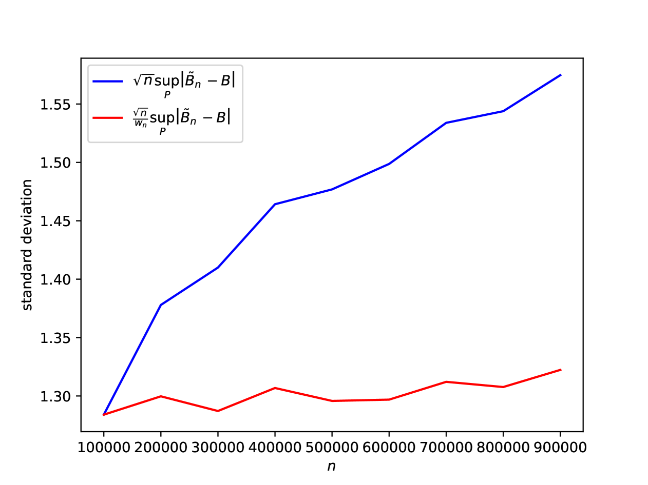
Figure 13: Uniformity of the penalized estimator: continuous vicinitiy of a flat face

From Figure 13, it appears that standard deviations multiplied by $\sqrt{n}$ are indeed exploding, although very slowly, while those multiplied by $\sqrt{n}/w_{n}$ are stable. It may be the case that the rate of $\sqrt{n}/w_{n}$ is sharp uniformly.

We next consider the grid that includes the flat face itself, but restricts the measures from approaching it from the left and right. In other words, we conduct the same simulation exercise with:

$$\mathcal{G}_{n}\equiv\{-0.1,0,0.1\}\cup\{-0.05(1+C_{1}n^{-1/2}),0.05(1+C_{1}n^{-1/2})\}\cup$$

$$\{-0.05(1+C_{2}w_{n}n^{-1/2}),0.05(1+C_{2}w_{n}n^{-1/2})\}\cup\{-0.05(1+C_{3}w_{n}^{-1}),0.05(1+C_{3}w_{n}^{-1})\}$$

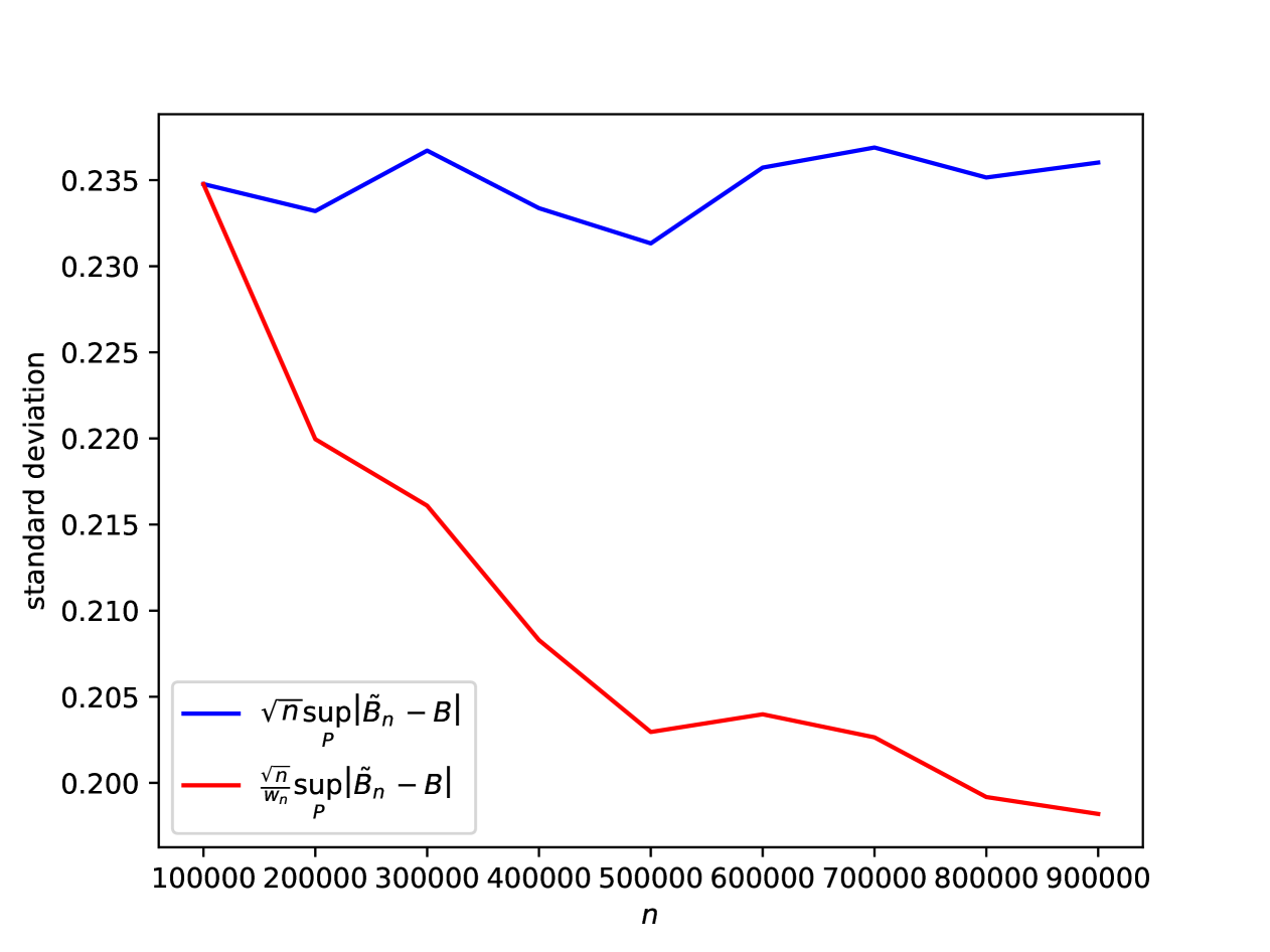
Figure 14: Uniformity of the penalized estimator: restricted vicinitiy of a flat face, flat face included.

In this case, Figure 14 suggests that uniform $\sqrt{n}$-consistency is achieved.

Finally, we return to the original grid $\mathcal{G}_{n}$, but consider the case in which Slater’s condition holds. For that reason, we take the true value of $d=0.5$ by sampling $d_{n}$ from $U[0,1]$ instead.

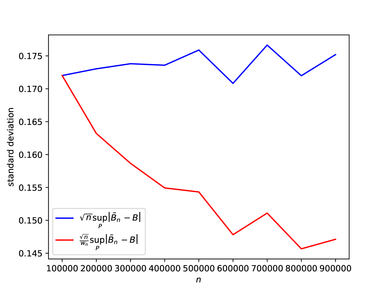
Figure 15: Uniformity of the penalized estimator: continuous vicinitiy of a flat face, Slater’s condition holds.

Once again, it appears that we obtain uniform $\sqrt{n}-$consistency.

Our simulation evidence thus suggests that while our estimator is only $\sqrt{n}/w_{n}$ uniformly consistent in general, it is $\sqrt{n}$-consistent uniformly apart from the sequences of probability measures, along which both Slater’s condition fails and where a flat-face is ‘approached’ monotonically. It appears possible to rule out the latter scenario by considering a uniform condition similar to the $\delta-$condition we imposed before. This condition would restrict the set of measures under consideration to those at which the ‘distance’ from a flat face is either $0$ or bounded away from $0$ in some metric. Accordingly, it would likely cover the unrestricted set of measures in the limit. These considerations, however, are the topic of a separate exploration, and space does not permit us to include them in this paper.

E.2. Irrelevance of $\overline{v}$

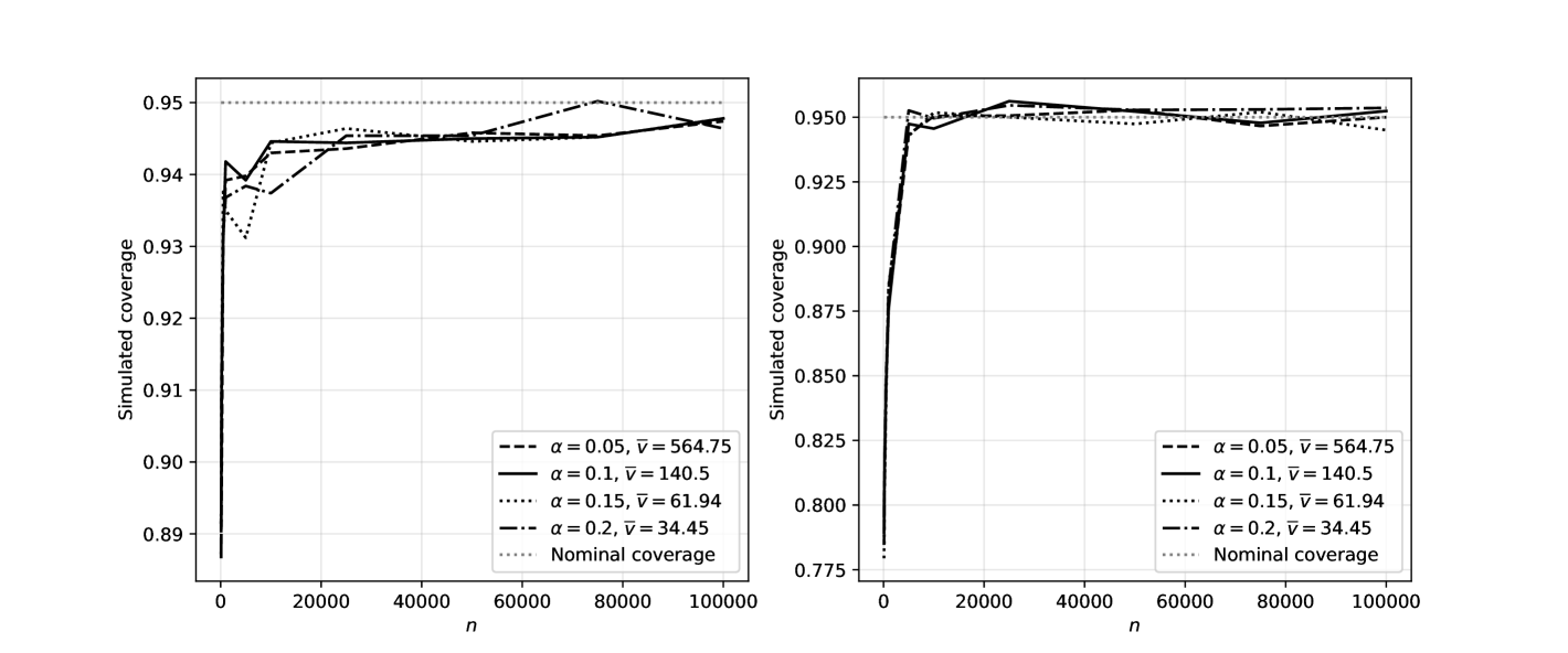
(a) Average coverage

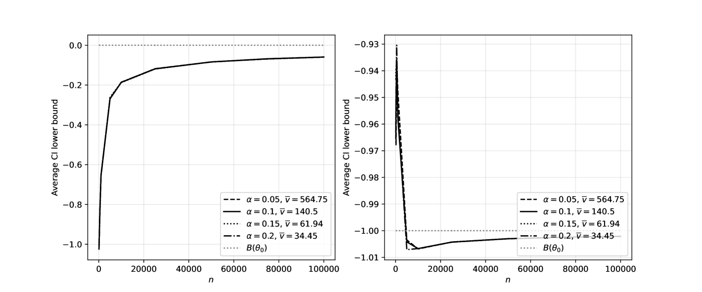
(b) Average CI lower bound

Figure 16: Debiased estimator’s performance for (14), simulated for $b=-0.05$ and $b=0$, left to right, different $\overline{v}$ corresponding to inverse $\alpha-$quantiles in Theorem H. $N_{sim}=5000$.

Observe that by non-emptiness of $\mathcal{S}_{A}$, there exists a $v\in\mathcal{S}_{A}$ such that $v=M_{A}^{\prime\dagger}p$. Thus, the scale of $v$ depends on the smallest singular value of $M^{\prime}_{A}$. It therefore seems reasonable to bound $v$ from above similarly to $w(\cdot)$, see Appendix H. We hence recommend setting $\overline{v}=\frac{d||p||}{\min_{i}||\hat{M}_{i\cdot}||\delta_{\alpha}}$ for some $\alpha$. Figure 16, however, suggests that a selection of $\overline{v}$ is not relevant, so long as it is large enough. We thus take $\alpha=0.1$ in our simulations, as it corresponds to a large $\overline{v}$.

Appendix F Alternative approach to inference

F.1. LP under Slater’s condition

One way to obtain a consistent estimator for the plug-in under SC is to employ the procedure developed in Hong and Li (2015). Let

$$\tilde{B}^{\prime}_{n}(\mathbb{Z}^{*}_{n})\equiv\frac{B(\hat{\theta}_{n}+\epsilon_{n}\mathbb{Z}^{*}_{n})-B(\hat{\theta}_{n})}{\epsilon_{n}}$$ (194)

For $\epsilon_{n}\to 0$ with $r_{n}\epsilon_{n}\to\infty$, we have the following proposition: If SC and Assumption B1 hold, and the bootstrapped $\mathbb{Z}^{*}_{n}$ satisfies the measurability conditions in Hong and Li (2015):

$$\underset{f\in BL_{1}(\mathbb{R})}{\sup}|\mathbb{E}[f(\tilde{B}^{\prime}_{n}(\mathbb{Z}^{*}_{n})))|\{X_{i}\}_{i=1}^{n}]-\mathbb{E}[f(B^{\prime}_{\theta_{0}}(\mathbb{G}_{0}))]|=o_{p}(1)$$ (195)

Assumption SC is rather strong, and one may not be comfortable imposing it directly. This is especially true in cases where many inequality restrictions are involved, such as under cMIV-s, because one would be concerned that the defined system may be close to point-identification. An even more serious problem in practice is that, even if an open ball is contained in $\Theta_{I}$ at $\theta_{0}$, the radius of that ball is not inconsequential in finite samples. A thinner identified set leads the bootstrap iterations of the N.D.M. to fail more often, as the constraint set turns empty at perturbed parameter values. Dropping the failed iterations introduces an unknown bias to the estimates, and so is not advised.

One potential solution would be to use the set-expansion estimator as in Section 4.2. Indeed, as long as the true system is feasible, expanding the set from the RHS renders the Slater’s condition true, and the procedure described in this section becomes applicable. The bias of such expansion would be controlled as follows:

$$\underset{\Theta_{I}}{\min}\leavevmode\nobreak\ p^{\prime}x-||p||d_{H}(\Theta_{I},\tilde{\Theta}_{I})\leq\underset{\tilde{\Theta}_{I}}{\min}\leavevmode\nobreak\ p^{\prime}x\leq\underset{\Theta_{I}}{\min}\leavevmode\nobreak\ p^{\prime}x$$ (196)

Moreover, by Lipschitz continuity of systems of linear inequalities, $d_{H}(\Theta_{I},\tilde{\Theta}_{I})\leq C|\kappa|$ for some $C>0$ depending on $\theta_{0}$, where the vector $\kappa>0$ is the RHS-expansion.

This estimator, however, would still be problematic both because it is conservative even in terms of the convergence rate, and because it relies on an arbitrarily selected set expansion. Since a larger expansion leads to a more conservative lower bound, in applied work the researcher would be tempted to select the minimal value that ensures the bootstrap iterations do not fail. The statistical properties of that approach are unclear.

F.2. Inference for the biased penalty

Observe that we can write $\tilde{B}\equiv\phi\circ\tilde{L}$, where $\tilde{L}(\theta)\equiv L(\cdot;\theta)$ is a map $\tilde{L}:\mathbb{R}^{S}\to\ell^{\infty}(\mathcal{X})$, and $\phi:\ell^{\infty}(\mathcal{X})\to\mathbb{R}$ is given by:

$$\phi(q)\equiv\underset{x\in\mathcal{X}}{\inf}\leavevmode\nobreak\ q(x),$$

and where we equip $\ell^{\infty}(\mathcal{X})$ with the sup norm. By Lemma S.4.9 in the Online Appendix of Fang and Santos (2018), $\phi$ is Hadamard directionally differentiable. It is therefore tempting to apply the chain rule to find the derivative of $\tilde{B}$, which only requires that $\tilde{L}$ is H.d.d. However, in the spirit of the example from Hansen (2017), this is not the case. The following remark illustrates that issue.

Remark F.1.

$g(y)(x)\equiv(x+y)^{+}$ viewed as a map $g:\mathbb{R}\to\ell^{\infty}(A)$ for $x\in A\equiv[-C;C]$ for some $C>0$ is not Hadamard directionally differentiable for any fixed $y\in[-C/2;C/2]$:

$$\underset{t_{n}\to 0^{+},h_{n}\to h}{\lim}||\frac{(y+x+t_{n}h_{n})^{+}-(y+x)^{+}}{t_{n}}-f(h)(x)||_{\infty}\neq 0$$

for any continuous $f(h)(x)$. To see that, note that the first term converges pointwise to $\mathds{1}\{y+x=0\}h^{+}+\mathds{1}\{y+x>0\}h$. Suppose that $h<0$ and consider: $x_{n}=-y-\frac{t_{n}}{2}h_{n}$, we have:

$$|\frac{(y+x_{n}+t_{n}h_{n})^{+}-(y+x_{n})^{+}}{t_{n}}-\mathds{1}\{y+x_{n}=0\}h^{+}+\mathds{1}\{y+x_{n}>0\}h|=$$

$$=o(1)-\frac{h}{2}\neq o(1)$$

In light of this finding, it should be almost surprising that $\tilde{B}(\cdot)$ is still Hadamard directionally differentiable, as we now demonstrate. Instead of using the chain rule, which is of course only a sufficient condition for differentiability, we notice that $\tilde{B}$ can be rewritten as a new linear program that has a non-empty interior of the constraint set. The penalty function estimator, $\tilde{B}(\theta;w)$ is Hadamard directionally differentiable in $\theta$ at $\theta_{0}$ if either i) $\mathcal{X}$ is a polytope with $Int(\mathcal{X})\neq\emptyset$, or ii) $\exists x\in\tilde{\mathcal{A}}(\theta_{0};w)\cap Int(\mathcal{X})$. The H.d.d. is given by:

$$\tilde{B}^{\prime}_{\theta_{0}}(h;w)=\underset{x\in\tilde{\mathcal{A}}(\theta_{0};w)}{\inf}\underset{\lambda\in\tilde{\Uplambda}(\theta_{0};w)}{\sup}h_{p}^{\prime}x+\sum_{j=1}^{2^{q}}\lambda_{j}\sum_{i\in\Pi_{j}}w_{i}(h_{c_{i}}-h^{\prime}_{M_{i}}x)$$ (197)

where $h=(h^{\prime}_{p},h_{c_{1}},\dots,h_{c_{q}},h^{\prime}_{M_{1}},\dots,h^{\prime}_{M_{q}})$ is the direction and an upper-hemicontinuous correspondence $\tilde{\Uplambda}:\mathbb{R}^{S}\to 2^{[2^{q}]}$ is as defined in the proof.

Proof.

Throughout this proof $w$ is taken to be fixed, therefore some dependencies on it are omitted in notation for brevity. We proceed in four steps:

1. Notice that $L(x;\theta,w)$ is a convex piecewise-linear function and it has the following representation:

   $$L(x;\theta,w)=\underset{j\in[2^{q}]}{\max}\leavevmode\nobreak\ \left\{p^{\prime}x+\sum_{i\in\Pi_{j}}w_{i}(c_{i}-M_{i}^{\prime}x)\right\},$$ (198)

   where $\{\Pi_{j}\}^{2^{q}}_{j=1}=2^{[q]}$, so that $\Pi_{j}$ for different $j$ contain indices of all possible combinations of positive penalty term. At a given $x$ these can be interpreted as the sets of violated constraints. Let $g_{j}(x,\theta)\equiv p^{\prime}x+\sum_{i\in\Pi_{j}}w_{i}(c_{i}-M_{i}^{\prime}x)$ for $j\in[2^{q}]$.

   The initial estimator can then be represented as:

   $$\tilde{B}(\theta;w)=\underset{x\in\mathcal{X}}{\min}\underset{j\in[2^{q}]}{\max}\leavevmode\nobreak\ g_{j}(x,\theta)$$ (199)

2. Assumptions i) or ii) allow us to impose w.l.g. that the known compact set $\mathcal{X}$ is a fixed, non-empty and bounded polyhedron. To see that for ii), note that the program is convex and therefore the sets of local and global minima coincide. If there exists an interior local minimum, it means that expanding the constraint set does not change the value, and therefore we can set $\mathcal{X}$ to be some compact and non-empty polyhedron that contains the original set. Then, another representation of the considered problem follows:

   $$\tilde{B}(\theta;w)=\underset{t,x}{\min}\leavevmode\nobreak\ t\quad\text{s.t.: }\begin{cases}t\in[\underline{t};\overline{t}]\\ x\in\mathcal{X}\\ g_{j}(x,\theta)\leq t,j\in[2^{q}]\end{cases}$$ (200)

   For some sufficiently wide $[\underline{t},\overline{t}]$, given $\theta$ is close to $\theta_{0}$ and such that $\tilde{B}(\theta_{0};w)\in(\underline{t},\overline{t})$. This is justified because $\tilde{B}(\theta;w)$ is continuous in $\theta$, as shown in the proof of Proposition 5.

3. Note that the constraint set of (200) is compact, non-empty at $\theta=\theta_{0}$ and, moreover, it contains an open set. To see that, consider some pair $x(\theta_{0}),t(\theta_{0})$ from the argmin of the problem, where $x(\theta_{0})\in\tilde{A}(\theta_{0};w)\subseteq\mathcal{X}$ and $t(\theta_{0})\equiv\tilde{B}(\theta_{0};w)$. Consider $\varepsilon\equiv\overline{t}-t(\theta_{0})$ and take $t^{*}\equiv t(\theta_{0})+\frac{\varepsilon}{2}$. Note that by definition $t(\theta_{0})\geq\max_{j}g_{j}(x(\theta_{0}))$. By continuity of $g_{j}(x,\theta_{0})$ in $x$ for all $j\in[2^{q}]$, $\exists\delta>0$ such that $t\geq\max_{j}g_{j}(x)$ $\forall t\in(t^{*}-\frac{\varepsilon}{4};t^{*}+\frac{\varepsilon}{4}),\forall x\in\mathbb{B}_{\delta}(x(\theta_{0}))$. By either i) or ii) $Int(\mathcal{X})\neq\emptyset$ and as $x(\theta_{0})\in\mathcal{X}$ it follows that $Int(\mathcal{X})\cap\mathbb{B}_{\delta}(x(\theta_{0}))$ is non-empty. It is also open as an intersection of two open sets. Therefore, the open set $\mathcal{O}\equiv(t^{*}-\frac{\varepsilon}{4};t^{*}+\frac{\varepsilon}{4})\times\left(\mathbb{B}_{\delta}(x(\theta_{0}))\cap Int(\mathcal{X})\right)$ is contained in the constraint set of the induced LP at $\theta_{0}$. That is, the problem at $\theta_{0}$ satisfies the Slater’s condition and Lemma 6 applies.

4. Suppose $\check{\Uplambda}(\theta_{0})$ is the set of Lagrange multipliers of (200) at $\theta=\theta_{0}$, and $\tilde{\Uplambda}(\theta_{0})$ is its projection on the coordinates corresponding to the constraints of form $g_{j}(x;\theta_{0})\leq t$ for all $j\in[2^{q}]$. A typical element of $\tilde{\Uplambda}(\theta_{0})$ will be written as $\lambda=(\lambda_{j})^{2^{q}}_{j=1}$. Recall that for $\theta$ in some small open neighbourhood of $\theta_{0}$ the value function of (200) is equal to $\tilde{B}(\theta;w)$ and, moreover, the problems are equivalent, so if $\check{\mathcal{A}}(\theta)$ is the $\arg\min$ of (200), then $\check{\mathcal{A}}(\theta)=\{\tilde{B}(\theta;w)\}\times\tilde{\mathcal{A}}(\theta;w)$. Using the conclusion of Step 3, direct application of Lemma 6 to (200) yields:

   $$\tilde{B}^{\prime}_{\theta_{0}}(h;w)=\underset{x\in\tilde{\mathcal{A}(\theta_{0};w)}}{\inf}\underset{\lambda\in\tilde{\Uplambda}(\theta_{0})}{\sup}\sum^{2^{q}}_{j=1}\lambda_{j}\left(h_{p}^{\prime}x+\sum_{i\in\Pi_{j}}w_{i}(h_{c_{i}}-h^{\prime}_{M_{i}}x)\right),$$ (201)

   where note that there are no terms corresponding to the objective function and the constraints $t\in[\underline{t},\overline{t}]$ and $x\in\mathcal{X}$, because there are no corresponding increments. Moreover, differentiating the Lagrangean of (200) and recalling that $t(\theta_{0})\in(\underline{t};\overline{t})$, so the constraints $t\in[\underline{t},\overline{t}]$ do not bind and the corresponding multipliers are $0$, one gets that $\forall\lambda\in\tilde{\Uplambda}(\theta_{0})$, we have $\sum^{2^{q}}_{j=1}\lambda_{j}=1$, establishing (197).

∎

Remark F.2.

By Lemma 2.1.a, Assumption A1 ensures ii) in the Proposition above if $\Theta_{I}\subseteq Int(\mathcal{X})$.

Assuming A1 holds, exact pointwise inference is then obtained via Proposition F.1. It is also straightforward to show that if A1 does not hold, but conditions i) or ii) in the Proposition above are otherwise satisfied, this inference is asymptotically conservative.

Computational considerations may be important in practice, especially as bootstrap is involved. In Appendix we further show that the penalty function estimator may be computed as a value of a simple LP. If there are $k$ constraints defining $\mathcal{X}$ and $q$ constraints for $\Theta_{I}$, with $d$ variables, the penalty-induced LP will feature $d+q$ variables and $2q+k$ constraints, which makes it almost as simple computationally as the usual plug-in estimator with $d$ variables and $q+k$ constraints.

F.3. Proof of Proposition 2.2.b

Definition (SMFCQ).

We say that Strict Mangasarian-Fromovitz Constraint Qualification (SMFCQ) holds at $\theta_{0}$ if $\exists x\in\mathcal{A}(\theta_{0})$ and the corresponding $\lambda\in\Uplambda(\theta_{0})$, such that i) $M_{\text{Supp}(\lambda)}$ has full row rank, and ii) there exists $z\in\mathbb{R}^{d}$ s.t. $M^{\prime}_{\text{Supp}(\lambda)}z=0$, and $M^{\prime}_{J(x;\theta_{0})\setminus\text{Supp}(\lambda)}z<0$.

It is well-known that SMFCQ is equivalent to $|\Uplambda(\theta_{0})|=1$ (see Proposition 1.1 in Kyparisis (1985) and Corollary 2.X in Mangasarian (1978)). We now prove Proposition 2.2.b.

Proof.

We first establish the following simple Lemma. Consider the extended real line $\overline{\mathbb{R}}\equiv\mathbb{R}\cup\{-\infty,+\infty\}$. Let $G:\mathbb{R}^{d_{y}}\to\overline{\mathbb{R}}$ be such that $G(y)\equiv\inf_{v\in V}y^{\prime}v$, where $V\subseteq\mathbb{R}^{d_{Y}}$ is non-empty. $G$ is linear iff $|V|=1$.

Proof.

The $\impliedby$ direction is obvious. For $\implies$, by contradiction, suppose that there exist $v_{0},v_{1}\in V$ such that $v_{0}\neq v_{1}$. Note that $G(0)=0$, and take some $y_{0}\in\mathbb{R}^{d_{y}}$ such that $(v_{0}-v_{1})^{\prime}y_{0}<0$. This can be done, because $v_{0}\neq v_{1}$. Because $G(y)\leq\min\{v_{0}^{\prime}y,v_{1}^{\prime}y\}$, we have $G(y_{0})\leq\min\{v_{0}^{\prime}y_{0},v_{1}^{\prime}y_{0}\}$, and by construction of $y_{0}$ we have $G(y_{0})<v_{1}^{\prime}y_{0}$. Similarly, $G(-y_{0})\leq\min\{v_{0}^{\prime}(-y_{0}),v_{1}^{\prime}(-y_{0})\}\leq v_{1}^{\prime}(-y_{0})$. Noting that by the above inequalities $G(y_{0})$ and $G(-y_{0})$ cannot be $+\infty$, we can add the inequalities getting $G(y_{0})+G(-y_{0})<v_{1}^{\prime}y_{0}+v_{1}^{\prime}(-y_{0})=0=G(0)$, which contradicts linearity of $G$. ∎

To prove the Proposition, we first observe that, under SC, i) and ii) are equivalent to $|\mathcal{A}(\theta_{0})|=|\mathcal{\Uplambda}(\theta_{0})|=1$. Note that i) is equivalent to $|\mathcal{A}(\theta_{0})|=1$ by definition. Suppose conditions i), ii) hold. Then, Proposition 1.1 in Kyparisis (1985) establishes $|\Uplambda(\theta_{0})|=1$. Conversely, suppose $|\mathcal{A}(\theta_{0})|=|\mathcal{\Uplambda}(\theta_{0})|=1$. Then, Proposition 1.1 in Kyparisis (1985) implies that SMFCQ must hold.

Thus, by Theorem 3.1 in Fang and Santos (2018), to prove the Proposition it suffices to show that, under SC, $B_{\theta_{0}}^{\prime}(h)$ is linear iff $|\mathcal{A}(\theta_{0})|=|\mathcal{\Uplambda}(\theta_{0})|=1$. Sufficiency is immediate.

To show necessity, denote the direction of the increment of $\theta$ by $h=(h_{p},h_{M},h_{c})$, where $h_{M}$ and $h_{c}$ have the shapes of $M$ and $c$ respectively. To see that it is necessary for the set of primary solutions to be a singleton, consider $h=(h_{p},0,0)$, i.e. set all components that correspond to $M$ and $c$ to $0$,

$$B_{\theta_{0}}^{\prime}(h)=\inf_{x\in\mathcal{A}(\theta_{0})}h^{\prime}_{p}x,$$

and apply Lemma F.3. Similarly, consider $h=(0,0,h_{c})$,

$$B_{\theta_{0}}^{\prime}(h)=\sup_{\lambda\in\Uplambda(\theta_{0})}\lambda^{\prime}h_{c},$$

and apply Lemma F.3 to observe that that $\Uplambda(\theta_{0})$ must be a singleton. This concludes the proof of the Proposition.

∎

F.4. LICQ is equivalent to $|\Uplambda(\theta_{0})|=1$ uniformly in $p$

Consider $\theta_{0}=(p^{\prime},\text{vec}(M)^{\prime},c^{\prime})^{\prime}$ satisfying A0 and fix some $\overline{x}\in\Theta_{I}(\theta_{0})$. Suppose $\tilde{\Theta}\equiv\{\tilde{\theta}\in\mathbb{R}^{S}|\tilde{\theta}=(\tilde{p}^{\prime},\text{vec}(M)^{\prime},c^{\prime})^{\prime},\text{ and }\overline{x}\in\mathcal{A}(\tilde{\theta}))\}$. Then,

$$|\Uplambda(\tilde{\theta})|=1\leavevmode\nobreak\ \forall\tilde{\theta}\in\tilde{\Theta}\iff\text{rk}M_{J(\overline{x};\theta_{0})}=|J(\overline{x};\theta_{0})|,\text{i.e. LICQ holds at $\overline{x}$.}$$

The claim above is also true if $\theta_{0}$ satisfies both A0 and SC.

Proof.

The implication $\impliedby$ is a well-known fact (see e.g. Gafarov (2024)). The other direction holds, because, setting the class of functions $\mathcal{F}$ in Wachsmuth (2013) to be the class of linear functions parametrized by $\tilde{\Theta}$, one observes that for $\tilde{p}=-\sum_{i\in J(\overline{x};\theta_{0})}M_{i}$, we have the corresponding $\tilde{\theta}\in\tilde{\Theta}$. The rest of the argument is identical to the proof of Theorem 2 in Wachsmuth (2013). ∎

Appendix G Set expansions approach

Proposition 2 highlights that the plug-in estimator fails whenever the constraint set has an empty interior. For completeness of our argument, we develop a natural alternative to the penalty function estimator - the set-expansion approach. The idea here is to enlarge $\Theta_{I}$ by relaxing each inequality constraint with a sequence $\kappa_{n}$. The resulting estimator has the flavor of the approach in Chernozhukov et al. (2007). Intuitively, it enforces SC at the cost of producing a potentially conservative estimate. We show that, in general, this estimator can indeed have a conservative rate, and thus we do not advocate its use in practice.

The approach in this section is first to prove that the appropriately extended identified set converges to the population identified set in Hausdorff distance, and then use uniform continuity of the criterion function as well as its resemblance to the support function to establish the convergence of the estimator itself.

Consider the following criterion function and its sample analogue:

$$Q(x)\equiv||(Mx-c)^{-}||^{2},\quad\hat{Q}_{n}(x)\equiv||(\hat{M}_{n}x-\hat{c}_{n})^{-}||^{2}$$

Denote the identified set as $\Theta_{I}\equiv\{x\in\mathcal{X}|Q(x)=0\}=\{x\in\mathcal{X}|Mx-c\geq 0\}$.

$||\hat{Q}_{n}(x)-Q(x)||_{\infty}\xrightarrow{p}0$, where $||\cdot||_{\infty}$ is over $\Theta_{I}$.

Proof.

$$|\hat{Q}_{n}(x)-Q(x)|=\left|\sum_{j}\left([\hat{M}_{n}x-\hat{c}_{n}]_{j}^{-}\right)^{2}-\left([Mx-c]_{j}^{-}\right)^{2}\right|=$$ (202)

$$=\left|\sum_{j}([\hat{M}_{n}x-\hat{c}_{n}]_{j}^{-}-[Mx-c]_{j}^{-})([\hat{M}_{n}x-\hat{c}_{n}]_{j}^{-}+[Mx-c]_{j}^{-})\right|\leq$$ (203)

$$\leq\sum_{j}|[\hat{M}_{n}x-\hat{c}_{n}]_{j}^{-}-[Mx-c]_{j}^{-}|\cdot|[\hat{M}_{n}x-\hat{c}_{n}]_{j}^{-}+[Mx-c]_{j}^{-}|\leq$$ (204)

$$\leq\left(\max_{j}\leavevmode\nobreak\ [\hat{M}_{n}x-\hat{c}_{n}]_{j}^{-}+[Mx-c]_{j}^{-}\right)\sum_{j}\left|\left[(\hat{M}_{n}-M)x+c-\hat{c}_{n}\right]_{j}\right|$$ (205)

Where (205) uses the fact that $|(y_{0})^{-}-(y_{1})^{-}|=|\max\{0,-y_{0}\}-\max\{0,-y_{1}\}|\leq|y_{0}-y_{1}|\leavevmode\nobreak\ \forall y_{0},y_{1}\in\mathbb{R}$. We now show that the last line converges to $0$ is supremum over $x\in\mathcal{X}$. Note that, since $\hat{M}_{n}\xrightarrow{p}M,\leavevmode\nobreak\ \hat{c}_{n}\xrightarrow{p}c$, the estimator asymptotically lies in any $\delta$-vicinity of the true population parameter. In other words, $\forall\delta>0$, we have $(\text{vec}(\hat{M}_{n})^{\prime},\hat{c}_{n}^{\prime})^{\prime}\in B_{\delta}((\text{vec}(M)^{\prime},c^{\prime})^{\prime})$ w.p. $1$ asymptotically.

Since $\mathcal{X}$ is a compact and because of the former result, both $\hat{M}_{n}x-\hat{c}_{n}$ and $Mx-c$ are bounded w.p. $1$ asymptotically, so there exists $K>0$ - large enough::

$$\underset{x\in\mathcal{X}}{\sup}\max_{j}\leavevmode\nobreak\ [\hat{M}_{n}x-\hat{c}_{n}]_{j}^{-}+[Mx-c]_{j}^{-}\leavevmode\nobreak\ \leq K+o_{p}(1)$$ (206)

Note that by Cauchy-Schwarz, $\sum_{j}\left|\left[(\hat{M}_{n}-M)x+c-\hat{c}_{n}\right]_{j}\right|\leq|\mathcal{F}_{t}|\cdot||(\hat{M}_{n}-M)x+c-\hat{c}_{n}||$. Further using (205), (206) and noting that for nonnegative $f,g$ one has $\sup_{A}fg\leq\sup_{A}f\cdot\sup_{A}g$, we get:

$$||\hat{Q}_{n}(x)-Q(x)||_{\infty}\leq(K+o_{p})\cdot|\mathcal{F}_{t}|\cdot\underset{x\in\mathcal{X}}{\sup}||(\hat{M}_{n}-M)x+c-\hat{c}_{n}||\leq$$ (207)

$$\leq(\tilde{K}+o_{p})\cdot\left(||\hat{M}_{n}-M||\cdot||x||_{\infty}+||c-c_{n}||\right)=o_{p}(1)$$ (208)

The proof is complete. ∎

Analogously to the proof of Lemma 3, one shows that because both $\hat{c}_{n}$ and $\hat{M}_{n}$ are $\sqrt{n}$-consistent from A0, we have:

$$\sup_{\mathcal{X}}(Q-\hat{Q}_{n})^{+}=O_{p}(1/\sqrt{n}),\quad\sup_{\Theta_{I}}\hat{Q}_{n}=O_{p}(1/n).$$

The plug-in estimator of the identified set, $\{x\in\mathcal{X}|\hat{Q}_{n}=0\}=\Theta_{I}(\hat{\theta}_{n})$, may not ‘cover’ the true asymptotically, as discussed in Chernozhukov et al. (2007) (CHT). To address that, consider the following class of set estimators:

$$\{x\in\mathcal{X}|n\hat{Q}_{n}(x)\leq\kappa_{n}\}$$

Fix $\kappa_{n}$ such that $P[\kappa_{n}\geq\sup_{\Theta_{I}}n\hat{Q}_{n}]\to 1$ and $\frac{\kappa_{n}}{n}\xrightarrow{p}0$. Let $\hat{\Theta}_{n}\equiv\{x|\hat{M}_{n}x-\hat{c}_{n}\geq-\frac{\sqrt{\kappa_{n}}}{\sqrt{n}}\iota\}$. It is the set that we want to prove consistent for the population identified set.

The issue is that the set $\hat{\Theta}_{n}$ is not a criterion-based set, so the results in CHT is not directly applicable. However, we can define $\underline{\Theta}_{n}\equiv\{x|\hat{Q}_{n}(x)\leq\frac{\kappa_{n}}{n}\}\subseteq\hat{\Theta}_{n}$ and $\overline{\Theta}_{n}\equiv\{x|\hat{Q}_{n}(x)\leq q\frac{\kappa_{n}}{n}\}\supseteq\hat{\Theta}_{n}$.

We then wish to ’sandwich’ $\hat{\Theta}_{n}$ between a smaller set that asymptotically covers $\Theta_{I}$ and a bigger set that is asymptotically covered by $\Theta_{I}$. The following simple lemma is an analogue of ‘sandwich theorem’ for sets.

Consider $\Theta_{I}\subseteq\mathcal{X}$ and suppose the random set $\hat{\Theta}_{n}\subseteq\Theta$ can be sandwiched between two sets: $\underline{\Theta}_{n}\subseteq\hat{\Theta}_{n}\subseteq\overline{\Theta}_{n}$, such that:

$$\underset{x\in\overline{\Theta}_{n}}{\sup}d(x,\Theta_{I})=o_{p}(1)$$

$$\underset{x\in\Theta_{I}}{\sup}d(x,\underline{\Theta}_{n})=o_{p}(1)$$

Then:

$$d_{H}(\hat{\Theta}_{n},\Theta_{I})=o_{p}(1)$$

Proof.

Writing out the definitions and applying CMT yields the result. ∎

The only thing that remains to show consistency of the set-estimator is to prove that the inequalities in Lemma G hold in our case. The derivation below follows the usual CHT logic. The first equality is established through:

$$P[\underset{x\in\overline{\Theta}_{n}}{\sup}d(\theta,\Theta_{I})\leq\varepsilon]=P[\overline{\Theta}_{n}\subseteq\Theta_{I}^{\varepsilon}]=$$ (209)

$$P[\overline{\Theta}_{n}\cap\mathcal{X}\setminus\Theta_{I}^{\varepsilon}=\emptyset]\geq P[\underset{x\in\overline{\Theta}_{n}}{\sup}Q(\theta)<\underset{x\in\mathcal{X}\setminus\Theta^{\varepsilon}_{I}}{\inf}Q(\theta)]$$

Then, by uniform continuity and by the construction of $\overline{\Theta}_{n}$:

$$\underset{x\in\overline{\Theta}_{n}}{\sup}Q(\theta)=\underset{x\in\overline{\Theta}_{n}}{\sup}\hat{Q}_{n}(\theta)+o_{p}(1)=q\frac{\kappa_{n}}{n}+o_{p}(1)=o_{p}(1)$$

By construction of $\Theta_{I}$ and continuity of $Q(\theta)$, $\exists\delta>0$: $\underset{x\in\mathcal{X}\setminus\Theta^{\varepsilon}_{I}}{\inf}Q(\theta)>\delta$. Thus, the RHS of (209) goes to 1. So, $\underset{x\in\overline{\Theta}_{n}}{\sup}d(x,\Theta_{I})=o_{p}(1)$.

The other side follows, as by construction $\underset{x\in\Theta_{I}}{\sup}\hat{Q}_{n}(x)\leq\frac{\kappa_{n}}{n}\implies\Theta_{I}\subseteq\underline{\Theta}_{n}$. So,

$$P[\underset{x\in\Theta_{I}}{\sup}d(\theta,\underline{\Theta}_{n})\leq\varepsilon]\geq P[\underset{x\in\Theta_{I}}{\sup}\hat{Q}_{n}(x)\leq\frac{\kappa_{n}}{n}]\xrightarrow{p}1$$

Therefore, using Lemma 3, we conclude that:

$$d_{H}(\hat{\Theta}_{n},\Theta_{I})\xrightarrow{p}0$$

The next step is to recall that if we have two convex, compact sets, $A,B$, the following holds:

$$d_{H}(A,B)=\underset{||y||\leq 1}{\max}|s(y,A)-s(y,B)|,$$

where $s(y,S)\equiv\underset{t\in S}{\max}\leavevmode\nobreak\ y^{\prime}t$ - the support function.

Using uniform convergence of the value function and combining all the results:

$$|\underset{x\in\hat{\Theta}_{n}}{\min}\hat{p}_{n}^{\prime}x-\underset{x\in\Theta_{I}}{\min}p^{\prime}x|=|\underset{x\in\hat{\Theta}_{n}}{\min}p^{\prime}x-\underset{x\in\Theta_{I}}{\min}p^{\prime}x|+o_{p}(1)=$$

$$=|s(-p,\Theta_{I})-s(-p,\hat{\Theta}_{n})|+o_{p}(1)\leq||p||d_{H}(\Theta_{I},\hat{\Theta}_{n})+o_{p}(1)\xrightarrow{p}0$$

This establishes the following proposition: Let $\kappa_{n}$ : $P[\kappa_{n}\geq\sup_{\Theta_{I}}n\hat{Q}_{n}]\to 1$ and $\frac{\kappa_{n}}{n}\xrightarrow{p}0$. Then the following estimator is consistent for the sharp lower bound:

$$\check{B}_{n}\equiv\underset{\hat{M}_{n}x-\hat{c}_{n}\geq-\sqrt{\frac{\kappa_{n}}{n}}\iota}{\min}\hat{p}^{\prime}_{n}x\xrightarrow{p}\underset{Mx-c\geq 0}{\min}p^{\prime}x$$

In practice, Chernozhukov et al. (2007) suggest to select some $\kappa_{n}$ that diverges sufficiently slowly with the sample size. We use $\sqrt{\kappa_{n}}\propto\ln{\ln{n}}$ in the simulations in Section 2.6. Under the Slater’s condition the naive estimator is consistent, i.e. one could set $\kappa_{n}=0$.

Although it seems intuitive that $\check{B}_{n}$ should converge at the rate $\sqrt{n\kappa^{-1}_{n}}$, deriving that result is outside the scope of this paper, because we do not advocate its use. It is immediate to see, however, that $\check{B}_{n}$ can converge as slowly as $\sqrt{n\kappa^{-1}_{n}}$. For that, consider (4) without the inequality $x_{2}\leq x_{1}$ and setting $\hat{b}_{n}=0$. The minimum is attained at $-1-\sqrt{\frac{\kappa_{n}}{n}}$. Our simulation evidence suggests that the set-expansion estimator can be quite conservative in practice, see Section 2.6.

Remark G.1.

Under SC, Hadamard directional differentiability of the LP value implies continuity, and so setting $\kappa_{n}=0$ yields a consistent estimator.

Appendix H Penalty parameter selection

In this section, we discuss the fundamental tradeoff involved in selecting the penalty parameter and propose an expression for it. Let us first take stock of the results in Section 2. Throughout this section, we interchangeably refer to $w$ as either a vector penalty, or a constant that induces the vector-penalty $w\iota$.

In general, for a fixed $w$, both versions of the penalty estimator estimate the population parameter $\tilde{B}(\theta_{0};w)$, and not necessarily $B(\theta_{0})$. Lemma 2.1.a guarantees that the two values coincide, if $w$ is component-wise larger than some KKT vector $\lambda^{*}\in\Uplambda(\theta_{0})$. It may actually be shown that this conclusion is sharp in a sense that there exists an example of $\theta_{0}$, such that if $w_{j}<\lambda_{j}^{*}$ for some $j\in[q]$ and all $\lambda^{*}\in\Uplambda(\theta_{0})$, then $\tilde{B}(\theta_{0};w)<B(\theta_{0})$.

Proposition 2.3 establishes that at any measure at least one $\lambda^{*}\in\Uplambda(\theta_{0})$ can be written as

$$\lambda_{J^{*}}^{*}=M^{\prime-1}_{J^{*}}p,\quad\lambda^{*}_{[q]\setminus J^{*}}=0,$$

for a subset $J^{*}\subseteq[q]$ with $M_{J^{*}}$ being a square invertible matrix.

Assumption U1 then defines a class of measures $\mathcal{P}^{\delta}$, over which the smallest singular value of $M_{J^{*}}$ for at least one such $J^{*}$ is bounded away from $0$ by $\delta>0$. Proposition 2.3 illustrates that the family $\{\mathcal{P}^{\delta}\}_{\delta}$ defines a covering of the unrestriced set $\mathcal{P}=\bigcup_{\delta>0}\mathcal{P}^{\delta}$. As we show later, U1 ensures that for any measure from $\mathcal{P}^{\delta}$ there exists a KKT vector $\lambda^{*}$ whose largest coordinate is bounded from above by $||p||\delta^{-1}$. Therefore, over the class $\mathcal{P}^{\delta}$, Assumption A1 holds uniformly for $w=w^{*}\equiv\iota||p||\delta^{-1}$.

On the one hand, a greater fixed $w$ ensures that the equality $\tilde{B}(\theta_{0}(\mathbb{P});w)=B(\mathbb{P})$ holds over a larger subset $\mathcal{P}^{\delta}$ of the unrestricted set of measures $\mathcal{P}$. In practice, a larger value of $w$ improves the performance of the penalty approach at ‘sharp’ measures, i.e. at those measures where all $\lambda^{*}$ are large, or where the (maximal across $J^{*}$) smallest singular value of $M_{J^{*}}$ is small. To see this, let us return to the example (4) with $b<0$. For large $n$, one estimates $\hat{b}_{n}\approx b<0$, resulting in a (unique) sample KKT vector $\hat{\lambda}_{n}\in\Uplambda(\hat{\theta}_{n})$ that is proportional to $-\hat{b}^{-1}_{n}$. If $w>\hat{\lambda}_{n}$, then the penalty estimator selects the correct optimum $x^{*}=(0,0)$ with $\tilde{B}(\hat{\theta}_{n};w)=\hat{B}(\hat{\theta}_{n};w)=B(\theta_{0})$. Thus, if the true $b<0$ is closer to $0$, a larger $w$ is required to establish the above equality in finite samples. This defines one side of the tradeoff involved in selecting $w$.

On the other hand, a greater fixed $w$ may worsen the performance of the penalty function approach at ‘blunt’ measures, at which SC also fails. By ‘blunt’ we mean the measures at which there exists a relatively small $\lambda^{*}\in\Uplambda(\theta_{0}(\mathbb{P}))$, or where the (maximal across $J^{*}$) smallest singular value of $M_{J^{*}}$ is large, so that a relatively small $w$ is required to ensure that $\tilde{B}(\theta_{0}(\mathbb{P});w)=B(\mathbb{P})$. This issue is manifested in our theoretical results in the form of the rate requirement for $w_{n}\to\infty$, namely $w_{n}/\sqrt{n}\to 0$. To illustrate this, suppose in (4) the true $b$ is fixed at $0$. Then, one can show that $w^{*}=\frac{-1+\sqrt{5}}{2}\iota\approx 0.62\iota$ suffices for condition A1 to hold. Suppose instead that the penalty is set at $\vec{w}=w\iota$. For any sample size $n$, with probability $0.5$ one estimates a negative $\hat{b}_{n}<0$, which results in a (unique) sample KKT vector $\hat{\lambda}_{n}\in\Uplambda(\hat{\theta}_{n})$ that is proportional to $-\hat{b}_{n}$. If $w>\hat{\lambda}_{n}$, then the penalty function estimators coincide with the plug-in $\tilde{B}(\hat{\theta}_{n};w)=\hat{B}(\hat{\theta}_{n};w)=B(\hat{\theta}_{n})=0\neq B(\theta_{0})=-1$ by Lemma 2.1.a. In this case, the incorrect minimum, $(0,0)$, is selected.

It is impossible to find any sequence $w_{n}$ that would allow for consistent estimation at all $b<0$ measures, as well as at $b=0$, i.e. over $b\in[\underline{b};0]$ for any $\underline{b}<0$. Lemma 2.3 shows that this problem is fundamental, and cannot be circumvented by any estimator.

We still wish to develop an estimator that is uniformly valid ‘in most cases’. In line with the previous discussion, we must impose an ad-hoc restriction on the class of measures under consideration. We impose such restriction in the form of a $\delta-$condition. This choice is motivated by the ad-hoc presumption that, in most economic applications, ‘sharp measures’ in the form of $b\approx 0^{-}$ in Example 2.1 appear more paradoxical than, for example, point-identified measures that correspond to $b=0$.

Consider a row-normalized version of the matrix $M$, denoted by $\tilde{M}$, that satisfies

$$\tilde{M}=D^{-1}M,$$ (210)

where $D=\text{diag}(\frac{||M_{1\cdot}||}{\sqrt{d}},\frac{||M_{2\cdot}||}{\sqrt{d}},\dots,\frac{||M_{q\cdot}||}{\sqrt{d}})$. The normalized matrix then has rows $\tilde{M}_{j\cdot}=\frac{\sqrt{d}M_{j\cdot}}{||M_{j\cdot}||}$. Notice that by considering the pair $\tilde{M},\tilde{c}$, where $\tilde{c}\equiv D^{-1}c$, we are not changing the true polytope $\Theta_{I}=\{x\in\mathbb{R}^{d}|Mx\geq c\}=\{x\in\mathbb{R}^{d}|\tilde{M}x\geq\tilde{c}\}$. Let us assume, in addition to U0, that over $\mathcal{P}$ the norms of rows of $M$ are uniformly bounded away from $0$, i.e. $\min_{j\in[q]}||M_{j\cdot}||>\underline{m}>0$.

Consider $\lambda^{*}$ from Proposition 2.3,

$$\lambda^{*}_{J^{*}}=M_{J^{*}}^{\prime-1}p=D_{J^{*}}^{-1}\underbrace{\tilde{M}^{\prime-1}_{J^{*}}p}_{\tilde{\lambda}}.$$

Using Lemma C.3, recalling that $\sigma_{k}(A)=\sigma_{k}(A^{\prime})$, as well as using $\sigma_{1}(\tilde{M}^{-1}_{J^{*}})=\sigma^{-1}_{d}(\tilde{M}_{J^{*}})$, we get the bound

$$\tilde{\lambda}\leq||\tilde{\lambda}||_{\infty}\iota\leq\iota\frac{||p||}{\sigma_{d}(\tilde{M}_{J^{*}})}$$

Because $D_{J^{*}}^{-1}$ simply rescales each row by a positive constant, it follows that

$$\lambda^{*}_{J^{*}}\leq\frac{||p||}{\sigma_{d}(\tilde{M}_{J^{*}})}D_{J^{*}}^{-1}\iota.$$

So, the following penalty vector satisfies A1 uniformly over $\mathcal{P}$,

$$w^{*}(\mathbb{P},n)\equiv\frac{w_{n}||p||}{\sigma_{d}(\tilde{M}_{J^{*}})}D^{-1}\iota=\left(\frac{w_{n}\sqrt{d}||p||}{\sigma_{d}(\tilde{M}_{J^{*}})||M_{j\cdot}||}\right)_{j\in[q]}$$ (211)

where $w_{n}\in\mathbb{R}$ with $w_{n}\geq 1$, and possibly $w_{n}\to\infty$ (albeit not necessarily) with $w_{n}/\sqrt{n}\to 0$.

If one knew $\sigma_{d}(\tilde{M}_{J^{*}(\mathbb{P})}(\mathbb{P}))$ for all $\mathbb{P}\in\mathcal{P}$, the otherwise infeasible $\tilde{B}(\hat{\theta}_{n};w^{*}(\mathbb{P},n))$ would yield a uniformly $\sqrt{n}-$consistent estimator over $\mathcal{P}$. Similarly, due to the continuity of $\tilde{B}(\theta;\cdot)$, if one could uniformly consistently estimate $\sigma^{-1}_{d}(\tilde{M}_{J^{*}(\mathbb{P})}(\mathbb{P}))$ over $\mathcal{P}$, using $\tilde{B}(\hat{\theta}_{n};\hat{w})$ with penalty $\hat{w}\equiv\frac{w_{n}||p||}{\hat{\sigma}_{d}(\tilde{M}_{\hat{J}^{*}})}\hat{D}^{-1}\iota$ for some $w_{n}>1$ subject to the above restrictions, would yield a uniformly consistent estimator of $B(\mathbb{P})$. However, the impossibility result in Theorem 2.3 implies that there can be no such estimator, and therefore, over $\mathcal{P}$,

$$\text{one cannot uniformly consistently estimate }\sigma^{-1}_{d}(\tilde{M}_{J^{*}(\mathbb{P})}(\mathbb{P})).$$

We are thus forced to impose an ad-hoc lower bound for $\sigma_{d}(\tilde{M}_{J^{*}(\mathbb{P})}(\mathbb{P}))$. For that, we need an assessment of what is ‘reasonable’ for the smallest singular value of a $d\times d$ matrix that is normalized by row. Consider the following result: [Tao and Vu (2010)] Let $\Xi_{d}$ be a sequence of $d\times d$ matrices with $[\Xi_{d}]_{ij}\sim\xi_{ij}$, independently across $i,j$ where $\xi_{ij}$ are such that $\mathbb{E}[\xi]=0$, $Var(\xi)=1$ and $\mathbb{E}[|\xi|^{C_{0}}]<\infty$ for some sufficiently large $C_{0}$, then,

$$\sqrt{d}\sigma_{d}(\Xi_{d})\xrightarrow{d}\aleph,$$

where $\aleph$ has the cdf

$$\mathbb{P}[\aleph\leq t]=1-e^{-t/2-\sqrt{t}}.$$

Remark H.1.

The distribution of mean-zero, unit-variance $\xi_{ij}$ in Theorem H is arbitrary, possibly discrete, and not necessarily identical across $i,j$.

Remark H.2.

Observe that for any $\Xi_{d}$ satisfying the hypothesis of Theorem H we have $\mathbb{E}[||(\Xi_{d})_{j\cdot}||^{2}]=d=||\tilde{M}_{j\cdot}||^{2}$.

We therefore propose to lower-bound $\sqrt{d}\sigma_{d}(\tilde{M}_{J^{*}})$ by an $\alpha-$quantile of the distribution $\Sigma$, which we denote by $\delta_{\alpha}$. Specifically, our recommendation for the penalty parameter is

$$w(\mathcal{D}_{n},n)\equiv\left(\frac{w_{n}d||p||}{\delta_{\alpha}||\hat{M}_{j\cdot}||}\right)_{j\in[q]},$$

where

$$\delta_{\alpha}=\left(\sqrt{1-2\ln(1-\alpha)}-1\right)^{2}.$$

We find that the pair $\alpha=0.2$ and $w_{n}=\frac{\ln\ln n}{\ln\ln 100}$ works well in our simulations.

Remark H.3.

If the value function was added to the constraints using the ‘trick’ from Gafarov (2024), the resulting matrix $\overline{M}$ and vector $\overline{c}$ are

$$\overline{M}=\begin{pmatrix}1&-p^{\prime}\\ 0&M\end{pmatrix},\overline{c}=\begin{pmatrix}0\\ c\end{pmatrix}$$

In the corresponding LP in population

$$\min_{t,x}(t\leavevmode\nobreak\ \leavevmode\nobreak\ x^{\prime})e_{1},\quad\text{s.t.: }t\geq p^{\prime}x,\leavevmode\nobreak\ Mx\geq c$$ (212)

under A0 it is straightforward to observe all $\overline{\lambda}\in\Uplambda(\theta_{0})$ that correspond to (212) with Proposition 2.3 applied to it, will have the form

$$\overline{\lambda}=\begin{pmatrix}1&0\\ -p&M^{\prime}_{J^{*}}\end{pmatrix}^{-1}e_{1}=\begin{pmatrix}1\\ M^{\prime-1}_{J^{*}}p\end{pmatrix},$$

where $J^{*}$ is the set from Proposition 2.3 applied to the original LP and the last equality follows by direct computation. So, when applying the penalty function approach to the problem (212), one should use

$$\overline{w}(\mathcal{D}_{n},n)=\begin{pmatrix}1\\ w(\mathcal{D}_{n},n)\end{pmatrix}.$$

Appendix I Identification under cMIV

Sharp identification results for cMIV conditions follow from Theorem 3.2. cMIV-w, however, allows for a more explicit characterization of the bounds, which may better illustrate the source of the identifying power of cMIV-w relative to MIV. This characterization is also useful in binary settings, when cMIV assumptions coincide. For didactic purposes, in this section we also show how to construct the restriction matrix $M$ and vector $c$ under cMIV-s, cMIV-p and MIV. While we focus on bounding potential outcomes, other choices of $\beta^{*}$ can be accommodated by applying Theorem 3.2.

In what follows, $I_{k}$ stands for the identity matrix of dimension $k$, and $\iota_{k}$ is the vector of ones of size $k$. These subscripts may be dropped in what follows without further notice. All vectors are column vectors, and $\mathbb{R}^{n\times m}$ refers to the space of real-valued $n\times m$ matrices. Notice that we can consider each $t\in\mathcal{T}$ separately, because cMIV conditions do not impose any restrictions across potential outcomes.

I.1. Recursive bounds under cMIV-w

Construct the ordering on the support of $Z$: $\mathcal{Z}=\{z_{1},z_{2},\dots,z_{N_{Z}}\}$, s.t. $z_{i}<z_{j}$ for $i<j$. Denote by $l_{i}(t),\leavevmode\nobreak\ u_{i}(t)$ the sharp lower and upper bounds for the conditional moment over the whole treatment support, $\mathbb{E}[Y(t)|Z=z_{i}]$. Similarly, let $l^{-t}_{i}(t),\leavevmode\nobreak\ u^{-t}_{i}(t)$ be the sharp upper and lower bounds for the counterfactual subset, $\mathbb{E}[Y(t)|T\neq t,Z=z_{i}]$. We shall suppress the dependence on $t$ whenever it does not cause confusion.

The only bound of interest is the bound on unconditional expectation, $l_{i}$. However, it turns out to be instructive to also consider the bound for the counterfactual subset, $l^{-t}_{i}$.

If i) cMIV-w holds or ii) treatment is binary and cMIV-s or cMIV-p hold, the sharp bounds for $\mathbb{E}[Y(t)|Z=z_{j}]$ are obtained through the following recursion for $j\geq 2$:

$$l_{j} =l_{j-1}+\Delta_{j}$$ (213)

$$l^{-t}_{j} =l^{-t}_{j-1}+\Delta^{-t}_{j}$$ (214)

Where $\Delta_{j},\Delta_{j}^{-t}\geq 0$ are defined as follows:

$$\Delta_{j} \equiv\left(\underbrace{\frac{\Delta P[T\neq t|Z=z_{j}]}{P[T\neq t|Z=z_{j-1}]}\left(l_{j-1}-P[T=t|Z=z_{j-1}]\mathbb{E}[Y(t)|T=t,Z=z_{j-1}]\right)}_{\text{$\Delta P[T\neq t|Z=z_{j}]l^{-t}_{j-1}$}}+\delta_{j}\right)^{+}$$ (215)

$$\Delta^{-t}_{j} \equiv\frac{1}{P[T\neq t|Z=z_{j}]}\left(-\Delta P[T\neq t|Z=z_{j}]l^{-t}_{j-1}-\delta_{j}\right)^{+}$$ (216)

$$\delta_{j} \equiv\Delta(P[T=t|Z=z_{j}]\mathbb{E}[Y(t)|T=t,Z=z_{j}])$$ (217)

Sharp upper bounds $u_{i},u_{i}^{-t}$ are obtained analogously. Moreover,

$$\sum_{i=1}^{N}P[Z=z_{i}]l_{i}(t)\leq\mathbb{E}[Y(t)]\leq\sum_{i=1}^{N}P[Z=z_{i}]u_{i}(t)$$ (218)

In the absence of additional information, these bounds are sharp.

Proof.

Note that $l^{-t}_{1}=K_{0}$ and $u^{-t}_{N}=K_{1}$. Moreover, $l_{1}=\mathbb{P}[T=t|Z=z_{1}]\mathbb{E}[Y(t)|T=t,Z=z_{1}]+\mathbb{P}[T\neq t|Z=z_{1}]K_{0}$, $u_{N}=\mathbb{P}[T=t|Z=z_{N}]\mathbb{E}[Y(t)|T=t,Z=z_{N}]+\mathbb{P}[T\neq t|Z=z_{N}]K_{1}$. First, we note that the equations above may be rearranged to yield:

$$l^{-t}_{j} =\max\left\{\frac{1}{P[T\neq t|Z=z_{j}]}\left(l_{j-1}-\mathbb{E}[Y(t)|T=t,Z=z_{j}]P[T=t|Z=z_{j}]\right),\leavevmode\nobreak\ l^{-t}_{j-1}\right\}$$ (219)

$$l_{j} =\mathbb{E}[Y(t)|T=t,Z=z_{j}]P[T=t|Z=z_{j}]+l^{-t}_{j}P[T\neq t|Z=z_{j}]$$ (220)

We consider the sharp lower bounds and proceed by induction on $j$. The proof for the sharp upper bounds is identical.
Consider $j=2$. The only information about lower bounds provided by assumption cMIV-w at $j=2$ is:

$$\begin{cases}\mathbb{E}[Y(t)|Z=z_{2}]\geq\mathbb{E}[Y(t)|Z=z_{1}]\\ \mathbb{E}[Y(t)|T\neq t,Z=z_{2}]\geq\mathbb{E}[Y(t)|T\neq t,Z=z_{1}]\end{cases}$$

Which can be rewritten as a single condition on $\mathbb{E}[Y(t)|T\neq t,Z=z_{2}]$:

$$\mathbb{E}[Y(t)|T\neq t,Z=z_{2}]\geq\max\Big{\{}\mathbb{E}[Y(t)|T\neq t,Z=z_{1}],$$

$$P[T\neq t|Z=z_{2}]^{-1}\big{(}\mathbb{E}[Y(t)|Z=z_{1}]-P[T=t|Z=z_{2}]\mathbb{E}[Y(t)|T=t,Z=z_{2}]\big{)}\Big{\}}$$

Because $l_{1}^{-t}$ is a sharp lower bound on $\mathbb{E}[Y(t)|T\neq t,Z=z_{1}]$, we get:

$$l_{2}^{-t} =\max\Big{\{}l_{1}^{-t},\leavevmode\nobreak\ P[T\neq t|Z=z_{2}]^{-1}\big{(}l_{1}-P[T=t|Z=z_{2}]\mathbb{E}[Y(t)|T=t,Z=z_{2}]\big{)}\Big{\}}$$

$$l_{2} =P[T=t|Z=z_{2}]\mathbb{E}[Y(t)|T=t,Z=z_{2}]+P[T\neq t|Z=z_{2}]l_{2}^{-t}$$

The base is thus proven. Now suppose that for some $j\geq 2$, and sharp lower bounds for $i<j$ are defined. The information we have at $j$ is:

$$\begin{cases}\mathbb{E}[Y(t)|Z=z_{j}]\geq\mathbb{E}[Y(t)|Z=z],\leavevmode\nobreak\ z<z_{j}\\ \mathbb{E}[Y(t)|T\neq t,Z=z_{j}]\geq\mathbb{E}[Y(t)|T\neq t,Z=z],\leavevmode\nobreak\ z<z_{j}\end{cases}$$

Or, equivalently,

$$\mathbb{E}[Y(t)|T\neq t,Z=z_{j}]\geq\max\Big{\{}\underset{i<j}{\max}\left\{\mathbb{E}[Y(t)|T\neq t,Z=z_{i}]\right\},$$

$$P[T\neq t|Z=z_{j}]^{-1}\big{(}\underset{i<j}{\max}\left\{\mathbb{E}[Y(t)|Z=z_{i}]\right\}-P[T=t|Z=z_{j}]\mathbb{E}[Y(t)|T=t,Z=z_{j}]\big{)}\Big{\}}$$

Because $l_{i},l_{i}^{-t}$ are sharp and non-decreasing in $i$ by inductive hypothesis, it follows that sharp lower bounds at $j$ are given by:

$$l_{j}^{-t} =\max\Big{\{}l^{-t}_{j-1},P[T\neq t|Z=z_{j}]^{-1}\big{(}l_{j-1}-P[T=t|Z=z_{j}]\mathbb{E}[Y(t)|T=t,Z=z_{j}]\big{)}\Big{\}}$$

$$l_{j} =\mathbb{E}[Y(t)|T=t,Z=z_{j}]P[T=t|Z=z_{j}]+l^{-t}_{j}P[T\neq t|Z=z_{j}]$$

The characterization in the proposition is obtained by rearranging these two equations.

To see that these bounds are indeed sharp, consider a process, for which $\mathbb{E}[Y(t)|T=d,Z=z_{j}]=l^{-t}_{j},d\neq t,j\in[N]$. For such process cMIV-w will hold by construction and $l_{j}$ and $l_{j}^{-t}$ are both attained for all $j$. An example of such process is given by:

$$Y(w)=\sum_{t}\mathds{1}\left\{t=w\right\}\left(\sum_{j}\left\{\mathds{1}\left\{Z=z_{j},T=t\right\}\eta(t)+\sum_{d\neq t}\mathds{1}\left\{Z=z_{j},T=d\right\}l_{j}^{-t}\right\}\right)$$ (221)

Where $\eta(t)$ is as defined in the proof of Theorem 1. ∎

The intuition for Proposition 2 is that MIV bounds are obtained by ’ironing’ the bounds on the population moment $\mathbb{E}[Y(t)|Z=z]$, which can be seen in equation (215). cMIV-w additionally ’irons’ the counterfactual moments $\mathbb{E}[Y(t)|T\neq t,Z=z]$, as evident from (216). Figure 1 plots the derived sharp bounds as well as the benchmark MIV sharp bounds for a simulation exercise.

I.2. Constructing $M$ and $c$ for cMIV-s and cMIV-p

We derive LP representations for cMIV family of assumptions.

Let $\mathcal{F}\equiv 2^{\mathcal{T}}\setminus\{\{t\},\emptyset\}$ and its cardinality, $Q\equiv|\mathcal{F}|=2^{N_{T}}-2$. Fix an ordering on $\mathcal{F}$, so that $\mathcal{F}=\{A^{1},A^{2},\dots A^{Q}\}$.

Then all information under cMIV-s can be written as:

$$\mathbb{E}[Y(t)|T\in A^{k},Z=z_{j}] \geq\mathbb{E}[Y(t)|T\in A^{k},Z=z_{j-1}],\leavevmode\nobreak\ k=1,\dots,Q,\leavevmode\nobreak\ j=2,\dots N_{Z}$$ (222)

$$\mathbb{E}[Y(t)|T=d,Z=z_{N}] \leq K_{1},d\in\mathcal{T}\setminus\{t\}$$ (223)

$$\mathbb{E}[Y(t)|T=d,Z=z_{1}] \geq K_{0},d\in\mathcal{T}\setminus\{t\}$$ (224)

Where notice that the LHS of (223) is the largest marginal moment due to monotonicity in $Z$, while the LHS of (224) is the smallest marginal moment. Therefore, once almost sure bounds for these two moments are imposed $\forall d\in\mathcal{T}\setminus\{t\}$, these are also implied for all other moments through equation (222) and the law of total probability.

We now rewrite the expectations in (222) in terms of pointwise conditional moments. Let the vector of unobserved treatment responses be $x^{j}\equiv\left(\mathbb{E}[Y(t)|T=d,Z=z_{j}]\right)^{\prime}_{d\neq t}$ and $p^{j}\equiv\left(P[T=d|Z=z_{j}]\right)^{\prime}_{d\neq t}$ be the vector of respective probabilities at $Z=z_{j}$. Denote the element of $x^{j}$ corresponding to $T=d$ as $x^{j}_{d}=\mathbb{E}[Y(t)|T=d,Z=z_{j}]$.

For $k=1,\dots,Q$ and $j=2,\dots,N_{Z}$, we can rewrite inequality (222) as follows:

$$\sum_{d\neq t}\mathds{1}\left\{d\in A^{k}\right\}\frac{P[T=d|Z=z_{j}]}{P[T\in A^{k}|Z=z_{j}]}x^{j}_{d}+$$

$$+\mathds{1}\left\{t\in A^{k}\right\}\frac{P[T=t|Z=z_{j}]}{P[T\in A^{k}|Z=z_{j}]}\mathbb{E}[Y(t)|T=t,Z=z_{j}]\geq$$

$$\geq\sum_{d\neq t}\mathds{1}\left\{d\in A^{k}\right\}\frac{P[T=d|Z=z_{j-1}]}{P[T\in A^{k}|Z=z_{j-1}]}x^{j-1}_{d}+$$

$$+\mathds{1}\left\{t\in A^{k}\right\}\frac{P[T=t|Z=z_{j-1}]}{P[T\in A^{k}|Z=z_{j-1}]}\mathbb{E}[Y(t)|T=t,Z=z_{j-1}]$$

Inequalities (223)-(224) are just $x^{N}_{d}\leq K_{1},d\neq t$ and $x^{1}_{d}\geq K_{0},d\neq t$. This can be written succinctly in matrix notation. Introdude the following:

$$G_{j} \equiv\left(\mathds{1}\left\{d\in A^{k}\right\}\frac{P[T=d|Z=z_{j}]}{P[T\in A^{k}|Z=z_{j}]}\right)_{k\in[Q],d\neq t}\in\mathbb{R}^{Q\times N_{T}-1}$$ (225)

$$c_{j} \equiv\left(\mathds{1}\left\{t\in A^{k}\right\}\frac{P[T=t|Z=z_{j}]}{P[T\in A^{k}|Z=z_{j}]}\mathbb{E}[Y(t)|T=t,Z=z_{j}]\right)_{k\in[Q]}\in\mathbb{R}^{Q}$$ (226)

The whole set of information given by cMIV-s can be represented as follows:

$$G_{j}x^{j}-G_{j-1}x^{j-1}\geq-\Delta c_{j},j=2,\dots,N_{Z}$$ (227)

$$x^{N}\leq K_{1}\iota$$ (228)

$$x^{1}\geq K_{0}\iota$$ (229)

The procedure for cMIV-p is similar. First, we note that all the information under it is given by:

$$\mathbb{E}[Y(t)|Z=z_{j}] \geq\mathbb{E}[Y(t)|Z=z_{j-1}],\leavevmode\nobreak\ j=2,\dots N_{Z}$$ (230)

$$\mathbb{E}[Y(t)|T=d,Z=z_{j}] \geq\mathbb{E}[Y(t)|T=d,Z=z_{j-1}],\leavevmode\nobreak\ d\in\mathcal{T}\setminus\{t\},\leavevmode\nobreak\ j=2,\dots N_{Z}$$ (231)

$$\mathbb{E}[Y(t)|T=d,Z=z_{N}] \leq K_{1},d\in\mathcal{T}\setminus\{t\}$$ (232)

$$\mathbb{E}[Y(t)|T=d,Z=z_{1}] \geq K_{0},d\in\mathcal{T}\setminus\{t\}$$ (233)

Where (230) is just MIV and (231) is the monotonicity of the pointwise conditional moments. In this case, we can once again represent all information in the matrix form (227)-(229) with the following matrices:

$$G_{j} \equiv\begin{pmatrix}p^{j\prime}\\ I_{N_{T}-1}\end{pmatrix}\in\mathbb{R}^{N_{T}\times N_{T}-1}$$ (234)

$$c_{j} \equiv\begin{pmatrix}P[T=t|Z=z_{j}]\mathbb{E}[Y(t)|T=t,Z=z_{j}]\\ 0_{N_{T}-1}\end{pmatrix}\in\mathbb{R}^{N_{T}-1}$$ (235)

Under cMIV-s, cMIV-p and MIV, sharp bounds on $\mathbb{E}[Y(t)]$ take the form:

$$\underset{Mx\geq c}{\min}\left\{\sum^{N}_{j=1}P[Z=z_{j}]\cdot p^{j\prime}x^{j}\right\}+\sum_{j=1}^{N}P[T=t,Z=z_{j}]\mathbb{E}[Y(t)|T=t,Z=z_{j}]\leq\mathbb{E}[Y(t)]\leq$$

$$\leq \underset{Mx\geq c}{\max}\left\{\sum^{N}_{j=1}P[Z=z_{j}]\cdot p^{j\prime}x^{j}\right\}+\sum_{j=1}^{N}P[T=t,Z=z_{j}]\mathbb{E}[Y(t)|T=t,Z=z_{j}],$$

where

$$M\equiv\left[\begin{array}[]{c c c c}-I_{N_{T}-1}&\dots&0&0\\ G_{N}&-G_{N-1}&\dots&0\\ \vdots&\ddots&\ddots&\vdots\\ 0&\dots&G_{2}&-G_{1}\\ 0&\dots&0&I_{N_{T}-1}\end{array}\right],\quad c\equiv\left(\begin{array}[]{c}-K_{1}\cdot\iota_{N_{T}-1}\\ -\Delta c_{N}\\ \vdots\\ -\Delta c_{2}\\ K_{0}\cdot\iota_{N_{T}-1}\end{array}\right),\quad x=\left(\begin{array}[]{c}x^{N}\\ \vdots\\ x^{1}\end{array}\right),$$ (249)

and $G_{j}$ and $c_{j}$ are given by (225) and (226) for cMIV-s and by (234) and (235) for cMIV-p. Under MIV, $G_{j}=p^{j\prime}$ and $c_{j}=P[T=t|Z=z_{j}]\mathbb{E}[Y(t)|T=t,Z=z_{j}]$.

I.3. Proof of Proposition 4.2

Let $\Gamma(z)\equiv\sum_{d\in\mathcal{T}}P[T=d|Z=z]\mathbb{E}[\psi(z,\eta)|Z=z]$.

1. Let $\tilde{g}(t)\equiv\mathbb{E}[g(t,\xi)|T=d,Z=z]=\mathbb{E}[g(t,\xi)|Z=z]$, where we use independence of $\xi$ and $T,Z$.
   MIV implies:

   $$\mathbb{E}[Y(t)|Z=z]=\tilde{g}(t)+h(t)\Gamma(z)\leavevmode\nobreak\ -\leavevmode\nobreak\ \text{increasing}$$

   Since inequality is strict for some $z,z^{\prime}$, it follows that $h(t)\neq 0$ and $h(t)/h(d)>0$. Note that:

   $$\mathbb{E}[Y(t)|T=d,Z=z]-\tilde{g}(t)=\frac{h(t)}{h(d)}\left(\mathbb{E}[Y(d)|T=d,Z=z]-\tilde{g}(d)\right)$$ (250)

   Therefore, cMIV-p holds iff all observed moments are monotone.

2. Let $\tilde{g}(t,d)\equiv\mathbb{E}[g(t,\xi)|T=d,Z=z]$, where we use independence of $\xi$ and $T,Z$. We can write:

   $$\mathbb{E}[Y(t)|T=d,Z=z]-\tilde{g}(t,d)=\frac{h(t)}{h(d)}\left(\mathbb{E}[Y(d)|T=d,Z=z]-\tilde{g}(d,d)\right)$$ (251)

   Using b): ii) yields the result.

Appendix J Empirical analysis

The upper bound is estimated by considering the problem

$$-B_{u}(\theta_{0})\equiv\min_{x\in\mathcal{X}}-p^{\prime}x,\leavevmode\nobreak\ \quad\text{s.t.}\quad Mx\geq c.$$ (252)

Suppose the estimator for (252), obtained from Algorithm 1, is $-\breve{B}_{u}$. By Theorem 2.2.a,

$$\mathbb{P}\left[-B_{u}(\theta_{0})<-\breve{B}_{u}+\frac{\hat{q}_{1-\alpha/2}(Z_{u})}{\sqrt{n_{2}}}\right]=\alpha/2+o(1),$$

where $Z_{u}\equiv\sqrt{n_{2}}(-\breve{B}_{u}+B_{u}(\theta_{0}))$, and $\hat{q}_{1-\alpha/2}(Z_{u})$ is a consistent estimate of its $1-\alpha/2$ quantile, which we obtain according to Remark 2.7. Similarly defining $Z\equiv\sqrt{n_{2}}(\breve{B}-B(\theta_{0}))$ and $\hat{q}_{1-\alpha/2}(Z)$, we have

$$\mathbb{P}\left[B(\theta_{0})<\breve{B}-\frac{\hat{q}_{1-\alpha/2}(Z)}{\sqrt{n_{2}}}\right]=\alpha/2+o(1).$$

In line with the notation of Section 3, suppose the target parameter is $\beta^{*}$, and observe that for any confidence interval given by $(lb_{n},ub_{n})$, we have

$$\mathbb{P}[\beta^{*}\notin(lb_{n},ub_{n})]=\mathbb{P}[\beta^{*}<lb_{n}\cup\beta^{*}>ub_{n}]\leq\mathbb{P}[\beta^{*}<lb_{n}]+\mathbb{P}[\beta^{*}>ub_{n}]\leq$$

$$\mathbb{P}[B(\theta_{0})<lb_{n}]+\mathbb{P}[B_{u}(\theta_{0})>ub_{n}],$$

where the penultimate inequality is a union bound, while the last inequality follows from $\beta^{*}\in[B(\theta_{0});B_{u}(\theta_{0})]$. Setting $ub_{n}\equiv\breve{B}_{u}-\frac{\hat{q}_{1-\alpha/2}(Z_{u})}{\sqrt{n_{2}}}$ and $lb_{n}\equiv\breve{B}-\frac{\hat{q}_{1-\alpha/2}(Z)}{\sqrt{n_{2}}}$ thus yields a valid two-sided CI for $\beta^{*}$, as

$$\mathbb{P}[\beta\notin(lb_{n},ub_{n})]\leq\alpha+o(1).$$

We drop outliers based on the first and the last percentiles by wage and set the bounds on the outcomes to be $K_{0}=4$ and $K_{1}=13$. By comparison, the observed range of values in the processed dataset is $(7.36;10.81)$.

	$ATE$(3, 2)	$ATE$(2, 1)	$ATE$(1, 0)
cMIV-s	(0.055, 3.781)	(0.089, 3.777)	(0.101, 3.75)
	{0.046, 3.798}	{0.079, 3.799}	{0.093, 3.77}
cMIV-p	(0.035, 4.165)	(0.041, 4.157)	(0.055, 4.054)
	{0.026, 4.174}	{0.033, 4.194}	{0.049, 4.077}
cMIV-w	(-0.004, 4.166)	(0.01, 4.08)	(-0.004, 4.101)
	{-0.014, 4.174}	{0.002, 4.094}	{-0.012, 4.118}
MIV	(0.002, 4.169)	(0.001, 4.24)	(0.001, 4.117)
	{-0.008, 4.178}	{-0.005, 4.251}	{-0.009, 4.125}
ETS	0.092	0.012	0.017

Table 2: Estimation results under various assumptions. See the code for more details.

References

- Aliprantis and Border (2007) Aliprantis, C. and K. Border (2007): Infinite Dimensional Analysis: A Hitchhiker’s Guide, Springer.
- Andrews (1999) Andrews, D. W. (1999): “Estimation when a parameter is on a boundary,” Econometrica, 67, 1341–1383.
- Andrews (2000) Andrews, D. W. K. (2000): “Inconsistency of the Bootstrap When a Parameter is on the Boundary of the Parameter Space,” Econometrica, 68, 399–405.
- Andrews et al. (2023) Andrews, I., J. Roth, and A. Pakes (2023): “Inference for Linear Conditional Moment Inequalities,” The Review of Economic Studies, 90, 2763–2791.
- Angrist and Chen (2011) Angrist, J. D. and S. H. Chen (2011): “Schooling and the Vietnam-era GI Bill: Evidence from the draft lottery,” American Economic Journal: Applied Economics, 3, 96–118.
- Angrist et al. (1996) Angrist, J. D., G. W. Imbens, and D. B. Rubin (1996): “Identification of causal effects using instrumental variables,” Journal of the American statistical Association, 91, 444–455.
- Beresteanu and Molinari (2008) Beresteanu, A. and F. Molinari (2008): “Asymptotic properties for a class of partially identified models,” Econometrica, 76, 763–814.
- Bertsekas (1975) Bertsekas, D. P. (1975): “Necessary and sufficient conditions for a penalty method to be exact,” Mathematical programming, 9, 87–99.
- Bhattacharya (2009) Bhattacharya, D. (2009): “Inferring optimal peer assignment from experimental data,” Journal of the American Statistical Association, 104, 486–500.
- Blundell et al. (2007) Blundell, R., A. Gosling, H. Ichimura, and C. Meghir (2007): “Changes in the distribution of male and female wages accounting for employment composition using bounds,” Econometrica, 75, 323–363.
- Boes (2009) Boes, S. (2009): “Bounds on counterfactual distributions under semi-monotonicity constraints,” Working Paper.
- Brand and Xie (2010) Brand, J. E. and Y. Xie (2010): “Who Benefits Most from College?: Evidence for Negative Selection in Heterogeneous Economic Returns to Higher Education,” American Sociological Review, 75, 273–302, pMID: 20454549.
- Card (1993) Card, D. (1993): “Using geographic variation in college proximity to estimate the return to schooling,” .
- Chernozhukov et al. (2007) Chernozhukov, V., H. Hong, and E. Tamer (2007): “Estimation and Confidence Regions for Parameter Sets in Econometric Models,” Econometrica, 75, 1243–1284.
- Chernozhukov et al. (2013) Chernozhukov, V., S. Lee, and A. M. Rosen (2013): “Intersection Bounds: Estimation and Inference,” Econometrica, 81, 667–737.
- Chetverikov (2019) Chetverikov, D. (2019): “Testing Regression Monotonicity in Econometric Models,” Econometric Theory, 35, 729–776.
- Cho and Russell (2023) Cho, J. and T. M. Russell (2023): “Simple Inference on Functionals of Set-Identified Parameters Defined by Linear Moments,” Journal of Business & Economic Statistics, 0, 1–16.
- Cygan-Rehm et al. (2017) Cygan-Rehm, K., D. Kuehnle, and M. Oberfichtner (2017): “Bounding the causal effect of unemployment on mental health: Nonparametric evidence from four countries,” Health Economics, 26, 1844–1861.
- De Haan (2017) De Haan, M. (2017): “The Effect of Additional Funds for Low-ability Pupils: A Non-parametric Bounds Analysis,” The Economic Journal, 127, 177–198.
- Demyanov (2009) Demyanov, V. F. (2009): Minimax: directional differentiability, Boston, MA: Springer US, 2075–2079.
- Duan et al. (2020) Duan, Q., M. Xu, L. Zhang, and S. Zhang (2020): “Hadamard directional differentiability of the optimal value of a linear second-order conic programming problem,” Journal of Industrial and Management Optimization, 17, 3085–3098.
- Fang and Santos (2018) Fang, Z. and A. Santos (2018): “Inference on Directionally Differentiable Functions,” The Review of Economic Studies, 86, 377–412.
- Gafarov (2024) Gafarov, B. (2024): “Simple subvector inference on sharp identified set in affine models,” arXiv e-prints, arXiv–1904, conditionally Accepted at Journal of Econometrics, 2024.
- Gomez (2022) Gomez, N. (2022): “Returns to college education in Colombia,” Higher Education Policy, 35, 692–708.
- Grünbaum et al. (1967) Grünbaum, B., V. Klee, M. A. Perles, and G. C. Shephard (1967): Convex polytopes, vol. 16, Springer.
- Gundersen et al. (2012) Gundersen, C., B. Kreider, and J. Pepper (2012): “The impact of the National School Lunch Program on child health: A nonparametric bounds analysis,” Journal of Econometrics, 166, 79–91, annals Issue on “Identification and Decisions”, in Honor of Chuck Manski’s 60th Birthday.
- Hansen (2017) Hansen, B. E. (2017): “Regression kink with an unknown threshold,” Journal of Business & Economic Statistics, 35, 228–240.
- Heckman and Vytlacil (2005) Heckman, J. J. and E. Vytlacil (2005): “Structural equations, treatment effects, and econometric policy evaluation 1,” Econometrica, 73, 669–738.
- Heckman and Vytlacil (1999) Heckman, J. J. and E. J. Vytlacil (1999): “Local instrumental variables and latent variable models for identifying and bounding treatment effects,” Proceedings of the national Academy of Sciences, 96, 4730–4734.
- Hirano and Porter (2012) Hirano, K. and J. R. Porter (2012): “Impossibility Results for Nondifferentiable Functionals,” Econometrica, 80, 1769–1790.
- Hong and Li (2015) Hong, H. and J. Li (2015): “The numerical delta method and bootstrap,” Tech. rep., Working paper.
- Honoré and Lleras-Muney (2006) Honoré, B. E. and A. Lleras-Muney (2006): “Bounds in competing risks models and the war on cancer,” Econometrica, 74, 1675–1698.
- Honoré and Tamer (2006) Honoré, B. E. and E. Tamer (2006): “Bounds on parameters in panel dynamic discrete choice models,” Econometrica, 74, 611–629.
- Imbens and Angrist (1994) Imbens, G. W. and J. D. Angrist (1994): “Identification and Estimation of Local Average Treatment Effects,” Econometrica, 62, 467–475.
- Imbens and Manski (2004) Imbens, G. W. and C. F. Manski (2004): “Confidence Intervals for Partially Identified Parameters,” Econometrica, 72, 1845–1857.
- Kline and Tamer (2023) Kline, B. and E. Tamer (2023): “Recent Developments in Partial Identification,” Annual Review of Economics, 15, 125–150.
- Kline and Tartari (2016) Kline, P. and M. Tartari (2016): “Bounding the Labor Supply Responses to a Randomized Welfare Experiment: A Revealed Preference Approach,” American Economic Review, 106, 972–1014.
- Kreider et al. (2012) Kreider, B., J. V. Pepper, C. Gundersen, and D. Jolliffe (2012): “Identifying the effects of SNAP (food stamps) on child health outcomes when participation is endogenous and misreported,” Journal of the American Statistical Association, 107, 958–975.
- Kyparisis (1985) Kyparisis, J. (1985): “On uniqueness of Kuhn-Tucker multipliers in nonlinear programming,” Mathematical Programming, 32, 242–246.
- Lafférs (2019) Lafférs, L. (2019): “Bounding average treatment effects using linear programming,” Empirical economics, 57, 727–767.
- Lafférs (2013) Lafférs, L. (2013): “A note on bounding average treatment effects,” Economics Letters, 120, 424–428.
- Li (1993) Li, W. (1993): “The sharp Lipschitz constants for feasible and optimal solutions of a perturbed linear program,” Linear algebra and its applications, 187, 15–40.
- Mangasarian (1978) Mangasarian, O. (1978): “Uniqueness of solution in linear programming,” Tech. rep., University of Wisconsin-Madison Department of Computer Sciences.
- Manski (1997) Manski, C. F. (1997): “Monotone Treatment Response,” Econometrica, 65, 1311–1334.