Error Bounds on the Universal Lindblad Equation in the Thermodynamic Limit
Abstract
It is a central problem in various fields of physics to elucidate the behavior of quantum many-body systems subjected to bulk dissipation. In this context, several microscopic derivations of the Lindblad quantum master equation for many-body systems have been proposed so far. Among them, the universal Lindblad equation derived by Nathan and Rudner is fascinating because it has desired locality and its derivation seems to rely solely on the assumption that the bath correlation time is much shorter than the dissipation time, which is the case in the weak-coupling limit or the singular-coupling limit. However, it remains elusive whether errors due to several approximations in deriving the universal Lindblad equation keep small during the time evolution in the thermodynamic limit. Here, rigorous error bounds on the time evolution of a local quantity are given, and it is shown that, under the assumption of the accelerated dissipation in bulk-dissipated systems, those errors vanish in the weak-coupling limit or the singular-coupling limit after taking the thermodynamic limit.
I Introduction
The quantum Markov process with complete positivity is generally described by a quantum master equation of the Lindblad form [1, 2]. The Lindblad equation has widely been used to describe a small quantum system in contact with thermal reservoirs, especially in quantum optics [3, 4]. Recent interest is shifted to open quantum many-body systems in connection with quantum control utilizing dissipation [5, 6, 7, 8], noisy quantum computation [9, 10], and nonequilibrium statistical physics [11, 12, 13, 14, 15]. The Lindblad equation is also a fundamental tool to study such a many-body system. Recent theoretical studies on open quantum many-body systems are largely triggered by experimental progress, which enables us to introduce tunable dissipation in many-body setups [6, 5, 7, 8]. In addition to that, there is also a line of research based on the idea that weak dissipation can be utilized as a probe field to better understand a given quantum many-body system [16, 17].
New insights have been gained through recent theoretical studies on the many-body Lindblad dynamics. In particular, it is recognized that the operator scrambling dynamics [18, 19] has important implications for dissipative dynamics under bulk dissipation. The operator scrambling—or the operator spreading—implies that a local operator becomes highly nonlocal after quantum time evolution in the Heisenberg picture. In general, a nonlocal operator is more fragile to dissipation, and hence the dissipative decay is accelerated due to the operator growth [20], which was numerically confirmed in the decay of the Loschmidt echo fidelity that is faster than exponential [21]. As a consequence of such an amplification of the effect of bulk dissipation, we sometimes have a non-zero decay rate even in the dissipationless limit (the thermodynamic limit is taken first), which is known as the quantum Ruelle-Pollicott resonance [17, 22], or the anomalous relaxation [23, 24].
In this way, fundamental properties of many-body Lindblad equations have been investigated, but their theoretical grounds are not well established. It is highly desired to give a microscopic derivation of the Lindblad equation and understand under what condition its use is justified. A standard derivation of the Lindblad equation involves using the secular approximation [25] (it is also referred to as the rotating-wave approximation), and the derived equation is known as the Davies equation [26]. The Davies equation is rigorously derived from the unitary time evolution of the system and the environment when the system of interest is finite and the system-bath interaction is infinitesimally weak. However, it is later recognized that the secular approximation is not justified and gives unphysical results in the many-body setup [27, 28]. We have to go beyond the secular approximation to derive the Lindblad equation for open quantum many-body systems.
So far, based on different approximations, various derivations of the Lindblad equation for many-body systems have been proposed [29, 30, 27, 31, 32, 33, 34, 35]. Among them, the universal Lindblad equation (ULE) derived by Nathan and Rudner [31, 32] has remarkable feature. Firstly, it has desired locality [31, 35] in contrast to the Davies equation. Secondly, the ULE appears to be solely derived from the assumption that the bath correlation time is much shorter than the dissipation time, which is the case in the weak-coupling limit (the system-bath coupling is infinitesimally weak) [36, 26] or in the singular-coupling limit (the bath correlation time is infinitesimally short) [37, 2, 38]. No assumption on the timescale of the intrinsic dynamics of the system of interest is explicitly used. Thus, it is expected that the derivation safely applies to many-body systems.
Although the existing derivation of the ULE given in Ref. [31] is physically reasonable, it is not rigorous and it is uncertain whether errors induced by several approximations needed to derive the ULE are negligible. Nathan and Rudner [31] evaluated rigorous error bounds on the approximations, but there are two problems:
-
(i)
Their error bounds diverge in the thermodynamic limit for bulk dissipation (i.e. each site of the system is coupled to its own bath). Therefore, it remains unclear whether those approximations are justified in macroscopic systems.
-
(ii)
They evaluated the error at the level of the equations of motion. It is not proved that the error does not accumulate over time. Thus, it is uncertain whether the error keeps small during the time evolution.
The aim of this paper is to overcome these two difficulties. We consider a one-dimensional quantum spin system with local Hamiltonian in which each site is coupled to its own free-boson bath, and evaluate rigorous error bounds on the time evolution of a local quantity due to the approximations made in the derivation of the ULE. Under the assumption of the accelerated dissipation, which is expected to be a generic property of bulk-dissipated open quantum many-body systems [21, 20, 17], we show that the errors vanish uniformly in time when we take the weak-coupling limit or the singular-coupling limit after taking the thermodynamic limit. The ULE is therefore justified for arbitrarily long times in the thermodynamic limit.
To overcome the difficulty (i), we prove that the existing Lieb-Robinson bound [39] is applicable to the ULE. By using it, finite error bounds in the thermodynamic limit are obtained. To overcome the difficulty (ii), i.e. to obtain desired time-independent error bounds, we use the assumption of the accelerated dissipation. Roughly speaking, it states that the dissipative decay rate of a local operator in the Heisenberg picture increases with time and is eventually saturated at a value that is much larger than the initial decay rate. As we have already mentioned, it was argued that such an accelerated dissipation generically occurs due to the operator spreading [21, 20, 17]. This is not a mathematically proved fact, but is a reasonable assumption. We give its theoretical picture and numerical evidence under a local Lindblad dynamics.
The plan of the paper is as follows. Section II.1 introduces the microscopic setup. Section II.2 gives a summary of the main result presented in this paper. Section II.3 introduces theoretical methods used in deriving the main result: the Lieb-Robinson bound and the accelerated dissipation. The former is formulated as a rigorous inequality as is explained in Sec. III, whereas the latter is an assumption without mathematical proof. Section IV is devoted to a detailed account of the accelerated dissipation with an intuitive picture and numerical evidences. Section V reviews the microscopic derivation of the ULE following Nathan and Rudner [31]. Various approximations are introduced and the explicit expressions of their errors are given. Section VI derives error bounds on the approximations introduced in Sec. V. We see that the Lieb-Robinson bound and the accelerated dissipation lead to the main result presented in Sec. II.2. We conclude with discussion in Sec. VII.
II Summary of the main result
Before going on to the theoretical detail, we summarize the main result presented in this paper. We first explain the theoretical setup and then our main result and key theoretical methods.
II.1 Setup
Let us consider a one-dimensional quantum spin system defined on the set of sites . The result presented in this paper is straightforwardly extended to a -dimensional system. The Hamiltonian of the system of interest is denoted by . We assume that is local in the sense that it is written as
| (1) |
where is an operator acting nontrivially on sites near . For simplicity, we assume that are finite range: the diameter of the support of is not greater than a constant for any .
In this paper, we focus on a static Hamiltonian, but the following discussion is extended to a time-dependent Hamiltonian by making a slight modification.
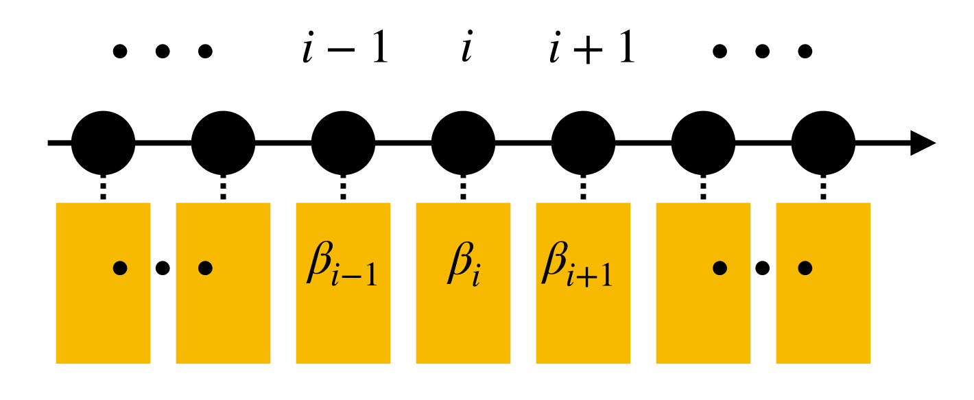
We consider bulk dissipation, see Fig. 1 for a schematic picture. Each site is coupled to its own bath consisting of free bosons, and hence the Hamiltonian of the baths is written as
| (2) |
where () is the creation (annihilation) operator of bosons interacting with the site . The interaction between the system and the baths is expressed by
| (3) |
where
| (4) |
is the bath operator, which is assumed to be linear in and , and is an Hermitian operator of the system that is normalized as ( is the operator norm). For simplicity, in the following, we assume that is a single-site operator, but it is straightforward to extend the result to an arbitrary local operator that acts nontrivially onto sites near . It is also straightforward to multiple dissipation channels at each site : as long as is finite.
The bath correlation function in the state
| (5) |
where is the inverse temperature of the th bath, is defined by
| (6) |
where
| (7) |
Without loss of generality, we can assume
| (8) |
The Fourier transform of is denoted by :
| (9) |
In an infinitely large bath, which we consider in the following analysis, is a continuous function of and vanishes in the long-time limit.
Following Nathan and Rudner [31], we introduce a jump correlator as
| (10) |
which is equivalent to
| (11) |
We introduce two positive constants and satisfying
| (12) |
for arbitrary and . From Eq. 12, we can derive the following inequality on :
| (13) |
Physically, and denote the strength of dissipation and the bath correlation time, respectively. It should be remarked that should satisfy , which is a consequence of the Kubo-Martin-Schwinger condition [40]: . The weak-coupling limit corresponds to the limit of with held fixed, whereas the singular-coupling limit corresponds to the limit of with held fixed.
Suppose a factorized initial state , where is the density matrix of the total system and is the reduced density matrix of the system of interest, which is defined as . We assume that is given by Eq. 5, i.e., each bath is in thermal equilibrium but its temperature can depend on site .
The density matrix of the total system obeys the Liouville-von Neumann equation
| (14) |
Formally, is expressed as
| (15) |
where . The exact reduced density matrix at time is thus given by , which is in general non-Markovian. By using various approximations, all of which are expected to be valid as long as , Nathan and Rudner [31] derived the following ULE:
| (16) |
where is the Liouvillian of the Lindblad form (it is also referred to as the Lindbladian). Here,
| (17) |
is the jump operator at site and , where
| (18) |
is the modification of the system Hamiltonian due to the coupling to the heat bath, which is called the Lamb-shift Hamiltonian [25]. In both of Eqs. 17 and 18, . In Sec. V, we briefly review the derivation of Sec. II.1 following Ref. [31].
For later convenience, we decompose into the unitary time evolution under and the effect of the coupling to the environment:
| (19) |
where . is further decomposed into the Lamb-shift part and the dissipative part :
| (20) |
Let us introduce the adjoint of , which is expressed as
| (21) |
The superoperator gives the time evolution of an operator in the Heisenberg picture: . It is noted that is a unital map: , where is the identity operator.
II.2 Main result
We consider the time evolution of a local operator that acts nontrivially to , where is finite ( denotes the number of elements of the set ). Without loss of generality, we can put .
We compare the exact time evolution of the expectation value , where is the exact reduced density matrix at time , with the approximate time evolution obeying the ULE: . We denote by the difference between the two:
| (22) |
which is interpreted as the error of the ULE.
What we are going to show is that is bounded from above by a constant , which depends on and but neither on time nor on the initial state , in the thermodynamic limit. Moreover, vanishes in the limit of or .
By introducing dimensionless constants and , where denotes the Lieb-Robinson velocity (it will be defined in Sec. III), it turns out that for small or small , which precisely means that for when is held fixed and for when is held fixed. Thus, our main result is summarized as follows:
| (23) |
For a sufficiently small value of or , the ULE is justified for arbitrarily long times even in the thermodynamic limit.
In a non-rigorous but physically sound derivation of the ULE [31] (see also Ref. [40] for a more informal derivation), it appears that the ULE is solely derived by the condition . However, the main result mentioned above implies that the condition of is not sufficient: a stronger condition is required for small .
II.3 Theoretical methods
We briefly explain key theoretical methods: the Lieb-Robinson bound and the accelerated dissipation.
The Lieb-Robinson bound is a mathematical bound on the speed of propagation of information in spin systems. It was originally proved for the unitary dynamics generated by a local Hamiltonian [41, 42, 43, 44], and later it was extended to Markovian open quantum systems [39, 45, 46]. Poulin [45] proved the Lieb-Robinson bound for open quantum systems described by a strictly local Lindbladian. Nachtergaele et al. [39] extended it to exponentially decaying ones.
The ULE generator of Sec. II.1 is, as it is, not written as a sum of exponentially decaying local terms, and hence it is not immediately obvious whether one can apply the result in Ref. [39] to the ULE. In Sec. III, we show that the Lieb-Robinson bound is valid for the ULE by showing that it can be further decomposed into exponentially decaying local terms.
The accelerated dissipation states that, under bulk dissipation, certain kinds of norms of a local operator decay at a rate increasing with time [21, 20, 17]. Eventually, the decay rate is saturated at a value much larger than the initial value. It occurs due to the combination of the operator spreading in the unitary time evolution [18, 19] and the presence of bulk dissipation. Although the accelerated dissipation is considered to be a generic phenomenon, it has not been given as a rigorous theorem.
In this paper, we assume an inequality, Eq. 39, representing the accelerated dissipation. We explain the statement of the accelerated dissipation and its intuitive picture in Sec. IV.1, and verify it numerically in Sec. IV.2. A large decay rate predicted by the accelerated dissipation is crucial to get an error bound that is uniform in time.
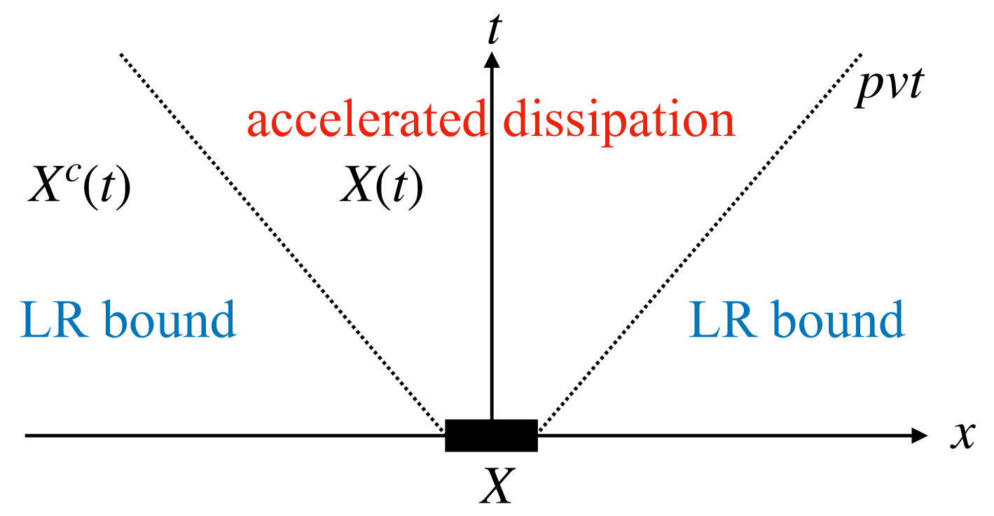
Figure 2 shows our strategy to evaluate the error bound. As we will see later in Sec. V, the error due to each approximation is expressed as a space-time summation. We decompose the spacetime into inside and outside of the light cone , where is a constant and is the Lieb-Robinson velocity. Outside the light cone, we use the Lieb-Robinson bound. Inside the light cone, instead, we use the accelerated dissipation.
III Lieb-Robinson bound for the ULE
Let us consider a time-dependent Lindbladian , whose adjoint is written as a sum of local terms:
| (24) |
where is a superoperator with support , i.e. for any operator whose support does not have intersection with : . For each , satisfies , but it is not necessary to assume that is the adjoint of a Lindbladian in its own right.
We assume that the Lindbladian is exponentially decaying, which implies
| (25) |
for any , where denotes the completely bounded norm [39, 47], and and are positive constants which are independent of the system size . Here, is the distance between sites and : in the open boundary condition and in the periodic boundary condition.
For the operator whose support is , let us define its dissipative time evolution in the Heisenberg picture as
| (26) |
where is the anti-time-ordering operation. We here put the superscript “d” to distinguish the unitary time evolution .
Under the conditions of Eqs. 24 and 25, the following Lieb-Robinson bound has been proved [39]:
| (27) |
where , , are positive constants which depend on the lattice geometry and constants and in Eq. 25 but not on the system size . Here, is the distance between the regions and .
It should be noted that the adjoint of the ULE Liouvillian, which is given by Sec. II.1 with Eqs. 17 and 18, is not in the form of Eq. 24 satisfying Eq. 25. It is therefore not obvious whether one can apply the Lieb-Robinson bound for the ULE. In the following, we show that the adjoint of the ULE Liouvillian can be brought into the form of Eq. 24 satisfying Eq. 25. It means that the Lieb-Robinson bound holds for Markovian time evolution obeying the ULE.
In the expression , is expressed in the desired form because is a local Hamiltonian by assumption. Therefore, the remaining task is to show that and can be decomposed into exponentially decaying local terms.
The operators and in the ULE are not strictly local because in Eqs. 17 and 18 become nonlocal for large . Considering the fact that the jump correlation function vanishes for , it is expected that in Eqs. 17 and 18 can be approximated by a strictly local operator . Here, we define as the restriction of to the region . More precisely, we define
| (28) |
where is the identity operator for the region . The operator is regarded as a local operator approximating . By using the Lieb-Robinson bound for the unitary time evolution and recalling that is a single-site operator with , we have
| (29) |
Let us define as the jump operator localized to the region by replacing in Eq. 17 by . We also define for with . By using Eqs. 29 and 12, it is shown that the operator norm of and are bounded from above as
| (30) |
and
| (31) |
where
| (32) |
This inequality leads to the following bound:
| (33) |
See Appendix A for the detail on the derivation of Eq. 31.
The dissipator is further decomposed into local terms as with
| (34) |
The completely bounded norm of is evaluated as
| (35) |
By using Eqs. 30 and III, we obtain
| (36) |
which shows that the dissipator of the ULE is exponentially decaying.
The Lamb-shift Hamiltonian is also decomposed into local terms as , where
| (37) |
Its operator norm is bounded as
| (38) |
This bound implies that the Lamb-shift Hamiltonian has exponentially decaying interactions.
In conclusion, the adjoint of the generator of the ULE can be written as a sum of exponentially decaying local terms. Therefore, we can apply the Lieb-Robinson bound of Sec. III to the time evolution obeying the ULE.
IV Accelerated dissipation
IV.1 Statement and intuitive picture
Let us consider the dissipative time evolution of a local operator in the Heisenberg picture: . We assume that is written in the form of Sec. II.1 with . We also assume that each is approximated by a local operator acting sites near (in the case of the ULE, Eq. 31 ensures this property).
Then, the statement of the accelerated dissipation is summarized as follows:
- Accelerated dissipation
-
Under the setup explained above, there exist positive constants and such that
(39) for any and , where is an arbitrary local operator and with being a local Hamiltonian.
In the following, we explain an intuitive picture behind this statement. Under bulk dissipation of strength , the decay rate of an operator is roughly proportional to , where is the average operator size of (i.e. how many sites this operator acts on) [21, 20, 17]. If the operator has no overlap with all the powers of the Hamiltonian , i.e. has no diagonal elements in the energy basis, roughly obeys the following equation [21, 20]:
| (40) |
where is the variance of the operator size. The first term of the right hand side implies that the operator size increases linearly , which is called operator spreading or operator growth [19, 18]. The second term shows that bulk dissipation decreases the operator size at a rate proportional to the variance of the operator size.
When there is no local conserved quantity at , which can happen for a time-dependent Hamiltonian , the operator size distribution evolves diffusively [21], and thus the operator size reaches the peak value , and then starts to decrease. In this case, up to , and then the operator eventually undergoes an exponential decay for . Here, is the spectral gap of the Liouvillian, which, interestingly, converges to a non-zero value in the weak dissipation limit after taking the thermodynamic limit: . This finite decay rate is related to the intrinsic relaxation of the system, which is referred to as the quantum Ruelle-Pollicott resonance [17, 22, 48, 49, 50, 51]. It is thus expected that Eq. 39 holds for a time-dependent Hamiltonian with no local conserved quantity at .
In contrast, when there is a local conserved quantity at (the Hamiltonian is always conserved in a static system), the presence of slow hydrodynamic modes makes the operator-size distribution broad and leads to . As a result, from Eq. 40, the average operator size will be saturated: for . As was already mentioned, the decay rate is roughly proportional to . The above estimate of for a static system thus implies the following behavior:
| (41) |
The decay rate for small is enhanced () due to operator spreading, which is the meaning of the accelerated decay.
When has an overlap with local conserved quantities (e.g. the system Hamiltonian), taking the commutator with a local operator as in Eq. 41 is crucial for the accelerated dissipation. To investigate the effect of local conserved quantities, we decompose the operator into the diagonal part and the off-diagonal part in the energy basis: . We expect that Eq. 41 holds for the off-diagonal part: . While, the diagonal part does not spread because it is conserved under the unitary time evolution at , and hence one might be tempted to consider that it does not show the accelerated decay.
We now argue that the accelerated decay actually occurs for the operator norm of the commutator . For simplicity, we assume that there is no local conserved quantity apart from , and the system of interest obeys the eigenstate thermalization hypothesis [52, 53], which implies
| (42) |
up to an exponentially small error in , where is a smooth function. Physically, corresponds to the equilibrium average of at the energy density . We then have , where we have used the fact that commutes with . Performing the Taylor expansion of as
| (43) |
and using the inequality
| (44) |
we obtain
| (45) |
Here, we have assumed that the Taylor expansion of around converges absolutely, and a non-essential constant factor is dropped in Eq. 45. When is a local Hamiltonian, does not depend on the system size for any local operator , which implies
| (46) |
and hence the contribution from the conserved quantity (i.e. the diagonal part) is negligible in the thermodynamic limit. It should be emphasized that the operator norm does not vanish in the thermodynamic limit. Taking the commutator with a local operator is crucial in Eq. 39. In this way, the contribution from the overlaps with conserved quantities in Eq. 39 can be dropped in the thermodynamic limit. It is thus expected that Eq. 39 also holds in a static Hamiltonian.
A similar argument shows that the diagonal part is also negligible in considering the Frobenius norm , where . Without loss of generality, we can assume . It is shown that in the thermodynamic limit. That is why the accelerated decay has been observed in the Loschmidt echo fidelity [21, 20], which is equivalent to .
IV.2 Numerical verification
To support the theoretical argument given above, we provide numerical results verifying Eq. 39. Let us consider the Ising model in a tilted field in the periodic boundary condition:
| (47) |
where () denote the Pauli matrices at site . We set and following [54], for which the eigenstate thermalization hypothesis is numerically verified. Bulk dissipation is modeled by the two jump operators and at each site .
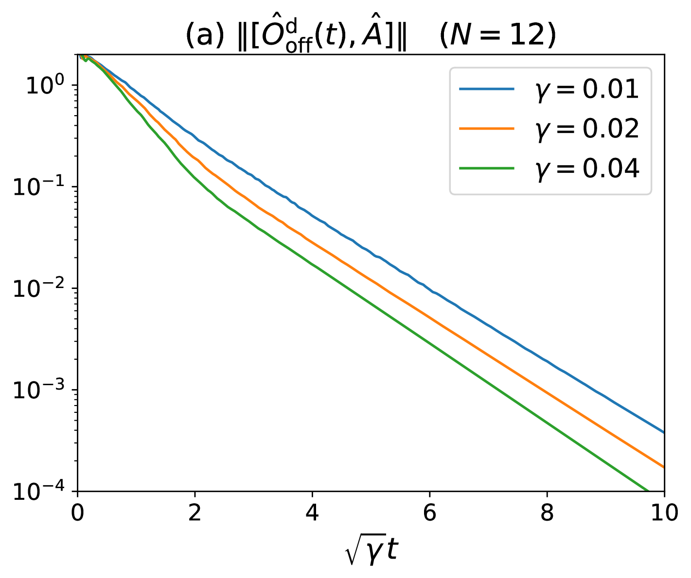
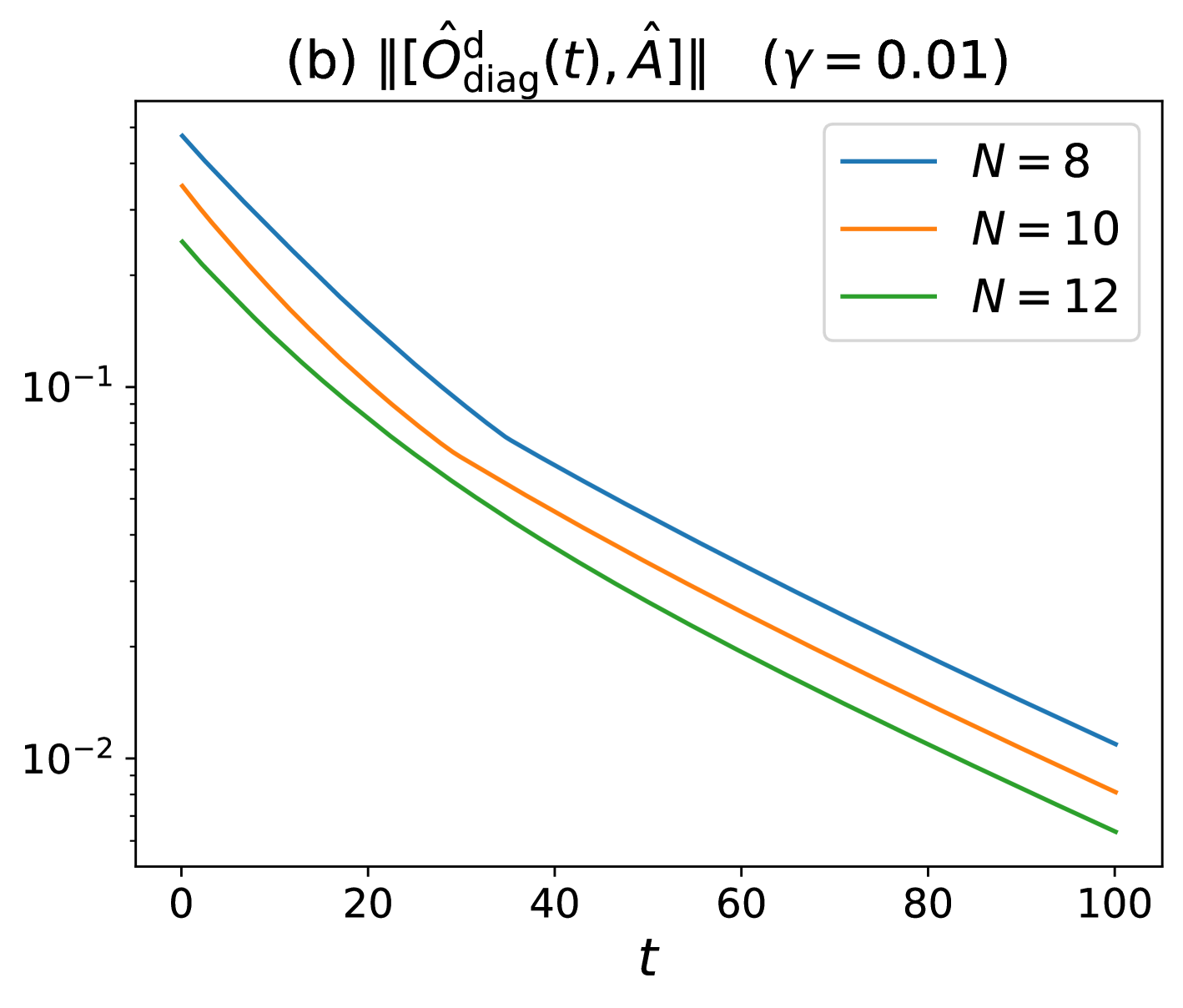
We choose and , and compute the norm appearing in Eq. 39. We decompose the norm into the diagonal part and the off-diagonal part . According to the discussion in Sec. IV, we expect that the norm from the off-diagonal part undergoes an exponential decay with the decay rate proportional to , and that the norm from the diagonal part decreases as the system size increases.
Our numerical results shown in Fig. 3 agree with those theoretical predictions. In Fig. 3 (a), the norm from the off-diagonal part is plotted as a function of for different values of . We see that the slope on a semi-log plot does not depend on , which implies , which is in accordance with Eq. 39. In Fig. 3 (b), the norm from the diagonal part is plotted for different system sizes. We see that the norm decreases as the system size increases, which agrees with the theoretical prediction . It means that the effect of conserved quantities would be negligible for large system sizes.
V Preliminary: derivation of the ULE
In this section, we review the derivation of Sec. II.1 following Ref. [31]. Through the derivation, we give the explicit expression of the error term for each approximation, which is used to evaluate the error bounds on the dynamics of a local quantity in Sec. VI.
Let us start with the Liouville-von Neumann equation for the total system, i.e., Eq. 14, and its formal solution given by Eq. 15 with a factorized initial state . In the interaction picture, , which is formally written as
| (48) |
where is the time-ordering operator and . Here, is the interaction Hamiltonian in the interaction picture, which is given by
| (49) |
where and .
In the interaction picture, we have
| (50) |
The reduced density matrix in the interaction picture is given by . By using Wick’s theorem for free bosons, we have
| (51) |
where and . That is, we multiply from left when and from right when .
Here, is rewritten as
| (52) |
By substituting it into Sec. V, we have
| (53) |
where
| (54) |
where
| (55) |
Ignoring corresponds to the Born approximation. Therefore, expresses the error induced by the Born approximation in the interaction picture.
Next, we perform the Markov approximation: in Sec. V, replace by and by . As a result, we obtain
| (56) |
where the error induced by the Markov approximation is given by
| (57) |
By introducing an operator
| (58) |
and using , Sec. V is expressed as
| (59) |
where . Equation 59 is known as the Redfield equation [25] when we ignore .
In a textbook derivation of the Lindblad equation [25], the secular approximation is used, but it is in general not valid in many-body systems, as is mentioned in Introduction. Nathan and Rudner [31, 32] introduce the memory-dressing transformation to derive the ULE, which is explained below.
Let us first rewrite Eq. 59 by using the jump correlation function, see Eq. 11. By using a superoperator , which is defined as
| (60) |
Eq. 59 is expressed as follows:
| (61) |
A key observation by Nathan and Rudner is that if we replace by , the above equation becomes of the Lindblad form, which is nothing but the ULE, except for the error term. To make a connection between the Redfield equation and the ULE, let us introduce the memory-dressing transformation , which is defined as
| (62) |
where
| (63) |
The transformed density matrix is referred to as the modified density matrix [31]. By differentiating Eq. 62 with respect to and using Eqs. 61 and V, we obtain
| (64) |
where
| (65) |
Straightforward calculations show that the first term of the right hand side of Eq. 64 is nothing but that of the ULE, i.e. Sec. II.1, in the interaction picture. The ULE Liouvillian in the interaction picture is given by
| (66) |
where recall that we write . We have
| (67) |
Equation 64 is thus written as
| (68) |
where
| (69) |
The modified density matrix obeys the ULE when we ignore
| (70) |
which is interpreted as the total correction to the ULE for the modified density matrix.
If the modified density matrix is close to the exact density matrix and is small enough, approximately obeys the ULE: by going back to the Schrödinger picture.
In Ref. [31], the following upper bounds on the trace norm of and that of are obtained 111Actually, Nathan and Rudner [31] considered the spectral norm, but we can repeat the same argument by using the trace norm without any change.:
| (71) |
and
| (72) |
respectively, where denotes the trace norm. Since , Eq. 71 implies that the correction term is actually small when . Under the same condition, Eq. 72 shows that we can ignore the difference between the exact density matrix and the modified one.
However, there are two problems in the above evaluation as is already pointed out in Introduction. Firstly, if we are interested in many-body systems under bulk dissipation, the condition is not satisfied in the thermodynamic limit (). Secondly, Eq. 71 gives an error bound at the level of the equations of motion, but errors might be accumulated with time. It is important to exclude this possibility to ensure that the ULE can be used to predict long-time (i.e. ) evolution of the system.
In the next section, we give an error bound on that is given by Eq. 22. It turns out that keeps small during the time evolution in the thermodynamic limit when or is small enough.
VI Error bounds
In this section, we derive the main result summarized in Sec. II. First of all, we decompose the total error into three parts by using the triangle inequality:
| (73) |
First term of the right hand side represents the error due to the difference between the exact density matrix and the modified one in the Schrödinger picture, . The second term represents the error due to the correction to the ULE for the modified density matrix, see Eq. 68. The last term represents the error due to the difference between the initial state of the exact density matrix and that of the modified one.
As for the second term of Sec. VI, by using the Schrödinger picture of Eq. 68, i.e.
| (74) |
where , we obtain
| (75) |
By further decomposing into , we have
| (76) |
where recall that . In this way, we can decompose the total error into the error due to each approximation: , where
| (Born approximation) | |||
| (77) | |||
| (Markov approximation) | |||
| (78) | |||
| (Memory-dressing transformation) | |||
| (79) |
In the following, we evaluate each error separately by using theoretical methods explained in Sec. II.3. It turns out that each error bound is at most for small or small .
VI.1 Born approximation
By using Sec. V and the cyclic property of the trace, and changing the integration variables as and , we obtain
| (80) |
By using Wick’s theorem, Eq. 13, and , we have
| (81) |
By using Eq. 13 again, is bounded as
| (82) |
Since the right hand side is an increasing function of , we obtain
| (83) |
It should be noted that this upper bound does not depend on . Therefore, if it is shown that is sufficiently small, the Born approximation is justified for arbitrarily long times.
In the following analysis, we change the integration variable to for notational simplicity. There is no confusion about it because does no longer depend on .
We introduce a region defined as
| (84) |
where is the Lieb-Robinson velocity and is an arbitrary constant satisfying (e.g. we can put ). In the following analysis, the summation over and in Sec. VI.1 is decomposed into the three contributions: (i) , (ii) and , and (iii) and . Correspondingly, . Below, we evaluate each contribution. In the following analysis, it turns out that the case (i) gives the dominant contribution, and we have .
(i)
In this case, we evaluate the double commutator in as
| (85) |
By using the assumption of the accelerated dissipation, i.e. Eq. 39,
| (86) |
where we used . A straightforward calculation yields
| (87) |
The dominant contribution to for small or small is thus given by
| (88) |
It should be noted that if we used a milder assumption , we would obtain , which does not tend to zero in the weak-coupling limit . To obtain the error bound that vanishes in the weak-coupling limit, the assumption of the accelerated decay, i.e. Eq. 39, is needed.
(ii) and
By using
| (89) |
where the Lieb-Robinson bound (Sec. III) is used in the last inequality, we have
| (90) |
By putting , we have and . We thus have
| (91) |
After carrying out the integrations, we obtain
| (92) |
which is of order and not dominant compared with for .
(iii) and
We introduce the region defined as
| (93) |
We then introduce the operator as the operator obtained by localizing to the region :
| (94) |
where is the complement of . Let us decompose in as follows:
| (95) |
By using the Lieb-Robinson bound, we have
| (96) |
where is the indicator function, and
| (97) |
By substituting Secs. VI.1 and VI.1 into Sec. VI.1, we obtain
| (98) |
As for , we choose 2 when , and choose when . As a result, we have
| (99) |
where
| (100) |
| (101) |
and
| (102) |
By introducing and , and replace the sum over and by integrations over and , we can explicitly evaluate , , and . We omit tedious calculations, and just present the result:
| (103) | ||||
By collecting them, for small or , which is not dominant compared with .
VI.2 Markov approximation
Let us start with the evaluation of the error caused by , which is given by
| (107) |
By using Eq. 39 (the accelerated dissipation) for with , and by using Sec. III (the Lieb-Robinson bound) for with , we find that it is bounded as
| (108) |
which is of order for small or .
Next, let us consider the error caused by . In Sec. VI.2, is written as
| (109) |
By introducing
| (110) |
we obtain
| (111) |
By using Wick’s theorem, is rewritten as
| (112) |
and thus its trace norm is evaluated as
| (113) |
By substituting Sec. VI.2 into Sec. VI.2, we have
| (114) |
Thus, the error caused by is given by
| (115) |
where we have used Sec. VI.2. We notice that the expression of is similar to that of given in Sec. VI.1, except for the presence of in front of .
Similarly to the analysis of the Born approximation, let us decompose the summation over and in Sec. VI.2 into the three parts : (i) , (ii) and , and (iii) and . In the following, we evaluate each contribution separately.
(i)
In this case, we have
| (116) |
This is identical to the upper bound on , and Eq. 87 also holds for . We therefore conclude
| (117) |
(ii) and
In this case, by using the simple bound and using the Lieb-Robinson bound, we have
| (118) |
This is identical to Eq. 90, and hence, following the same calculation, we conclude
| (119) |
(iii) and
By using and for arbitrary operators , , and , we have
| (120) |
By using this inequality, we obtain
| (121) |
where
| (122) |
and
| (123) |
We find that is identical to , and hence .
Thus, the remaining problem is to evaluate . The product in Sec. VI.2 is evaluated by using the Lieb-Robinson bound. We bound it as follows: when ,
| (124) |
where we used , and when ,
| (125) |
where we used (recall the definition of , see Eq. 93). By substituting these inequalities into Sec. VI.2, after calculations, we finally obtain
| (126) |
From this expression, we find that .
In conclusion, we find .
VI.3 Memory-dressing transformation
By going back to the Schrödinger picture, is given by
| (128) |
where is defined in Sec. V, which is expressed as
| (129) |
By using defined in Eq. 110, we can write
| (130) |
By substituting Eqs. 129 and 130 into Eq. 128, is bounded from above as
| (131) |
where
| (132) |
By using Eqs. 12 and VI.2, we obtain
| (133) |
By following similar calculations as in the previous subsections, an upper bound on is evaluated in Appendix B, where it turns out that
| (134) |
for small or small .
Next, we consider . By using , we obtain
| (135) |
where is the adjoint of : for arbitrary operators and . By using Eqs. 12, V and V combined with the inequality for an arbitrary , we obtain the following simple bound on :
| (136) |
where .
The evaluation of is provided in Appendix C. It turns out that the contribution from is dominant, and we again obtain
| (137) |
Next, let us consider . It is written as
| (138) |
By using Eqs. 129 and 12, we have
| (139) |
Let us evaluate it for and . For , we use Eq. 39. A straightforward calculation yields
| (140) |
The contribution from in the right hand side of Sec. VI.3 is thus given by
| (141) |
For , we use the Lieb-Robinson bound, e.g. Sec. III:
| (142) |
For , we use
| (143) |
and for , we use
| (144) |
We then obtain an upper bound
| (145) |
from in Sec. VI.3.
An upper bound on is given by the sum of Eqs. 141 and 145. We therefore find that behaves as
| (146) |
for small or small .
Finally, we consider . We find
| (147) |
which is identical to the right hand side of Eq. 138. We can therefore conclude that behaves as
| (148) |
for small or small .
VII Conclusion
The ULE describes dissipative time evolution of an open quantum many-body system. However, in its microscopic derivation, several approximations are introduced, and hence it has not been obvious at all whether the ULE gives accurate predictions, especially for the long-time behavior of macroscopically large quantum systems. In this paper, we evaluate errors on the time evolution of local quantities. For this purpose, we show that the Lieb-Robinson bound holds in an open system obeying the ULE, and introduce an assumption of the accelerated dissipation, which is physically motivated by recent works on the operator scrambling. The Lieb-Robinson bound and the accelerated dissipation are key tools to evaluate error bounds.
We find that the error is bounded from above by a quantity of order , where is the dimensionless dissipation strength and is the dimensionless correlation time of the environment. It is therefore concluded that either the weak-coupling limit or the singular-coupling limit justify the use of the ULE for arbitrarily long times in the thermodynamic limit.
Dissipation usually destroys quantum coherence, and hence it is crucial to understand the effect of dissipation and develop techniques reducing environmental effects in quantum technologies [10]. Meanwhile, recent experimental progress [5, 6, 7, 8] introduces a new perspective: engineered dissipation is rather useful to control and manipulate quantum states [56, 57]. The interplay between dissipation and interactions gives rise to rich nonequilibrium dynamics [13, 14] and new kinds of quantum phases [11, 58, 59]. It is important to develop new theoretical tools and lay the foundation for them to tame dissipation in quantum many-body systems. This work takes a step forward in this direction.
Finally, we conclude with open problems. The accelerated dissipation is used as a key assumption in this work: it is yet to be formulated as a mathematical theorem. It is an important future problem to refine the notion of the accelerated dissipation as a fundamental tool to describe open quantum many-body systems. It is also a future work to justify the Lindblad equation in boundary dissipated quantum many-body systems. The setup of boundary dissipation is relevant for quantum transport in a nonequilibrium steady state [60, 61]. In such a system, we typically observe delayed relaxation in the sense that the relaxation time is much larger than the inverse of the spectral gap of the Liouvillian [62, 63]. The delayed relaxation is considered to be originated from the presence of bulk hydrodynamic modes, which do not decay until they reach the boundary. It is then nontrivial how to control errors stemming from the inside of the light cone in Fig. 2. We hope to address these problems in the future.
Acknowledgements.
This work was supported by JSPS KAKENHI Grant No. JP21H05185 and by JST, PRESTO Grant No. JPMJPR2259.Appendix A Derivation of Eq. 31
The definition of the jump operator in the ULE is given in Eq. 17. By using it, we have
| (149) |
By using Eqs. 12 and 29, it is bounded as
| (150) |
Here, we decompose the integration range as , where we use in the former and in the latter. As a result,
| (151) |
dqzzq In the first term of the right hand side, , and hence
| (152) |
which is the desired inequality.
Appendix B Evaluation of
We evaluate an upper bound on
| (153) |
which is used to evaluate given by Sec. VI.3. For a fixed , the sum over and is decomposed into the three parts: (i) , (ii) and with , and (iii) and with . Each contribution is denoted by , , and , respectively.
(i)
In this case, we can simply evaluate as
| (154) |
Here, we use the acceleration of dissipation, i.e. Eq. 39:
| (155) |
(ii) and
In this case, is evaluated as
| (158) |
By putting , we have and . By using the Lieb-Robinson bound, we obtain
| (159) |
As for , when , we choose . When , we choose for , and 2 for . As a result, we obtain the following upper bound on :
| (160) |
By performing the integration over , we obtain
| (161) |
By substituting it into Sec. VI.3, after some calculations, we finally obtain , which corresponds to the contribution from with and , as follows:
| (162) |
For small or small , we find .
(iii) and
By using for arbitrary operators , , and , we have
| (163) |
By defining , we have
| (164) |
where is the operator that is obtained by localizing to the region defined by Eq. 93; see Eq. 94. By using the Lieb-Robinson bound, we have
| (165) |
where we have used , and
| (166) |
As for in Appendix B, the LR bound is used for when , and for when . We then have
| (167) |
where we used for and for .
By substituting above results, i.e. Appendices B, B, B and B, into Appendix B, we obtain an upper bound on and by using Sec. VI.3. Everything is finite, and we find
| (168) |
for small or small .
Appendix C Evaluation of
We evaluate , which is defined by Sec. VI.3. As before, we decompose the sum over into the three parts: (i) , (ii) and , and (iii) and . Each contribution is denoted by , , and .
(i)
(ii) and
Let us start with the expression
| (173) |
By putting , we do the following decompositions:
| (174) |
where
| (175) |
The operators and were introduced in Sec. III: they are operators localized to the region .
By substituting Eq. 174 into Appendix C, we obtain
| (176) |
As for , by using the inequality , which is obtained from the Lieb-Robinson bound, the operator norm is evaluated as
| (177) |
where . Next, as for in Appendix C, by using and , the Lieb-Robinson bound yields
| (178) |
where . As for , we can use Eq. 31:
| (179) |
Finally, as for and , by using and , we have
| (180) |
By collecting them, Appendix C is evaluated by approximating the sum over by the integral:
| (181) |
As a result, we find
| (182) |
for small or small .
(iii) and
In Sec. VI.3, by using , which is defined in Eq. 94, we have
| (183) |
We now decompose as
| (184) |
where is chosen as
| (185) |
and is defined by
| (186) |
for an arbitrary operator . See Secs. III and III for the definition of and , respectively. Appendix C is then bounded as
| (187) |
If we choose as in Eq. 185, the distance between the support of and the site is greater than (the former is under the condition ). Therefore, the Lieb-Robinson bound yields
| (188) |
Since
| (189) |
we have
| (190) |
where we have used and . By using Eqs. 36, III and 185, we find that there is a constant that depends solely on and such that
| (191) |
As for in Appendix C,
| (192) |
and the Lieb-Robinson bound implies
| (193) |
By collecting the above results, Appendix C leads to
| (194) |
By substituting it into Sec. VI.3 with the condition and , we can explicitly calculate an upper bound on . We do not give lengthy calculations here, but it turns out that the upper bound is finite and
| (195) |
for small or small .
References
- Lindblad [1976] G. Lindblad, On the generators of quantum dynamical semigroups, Commun. Math. Phys. 48, 119 (1976).
- Gorini et al. [1976] V. Gorini, A. Kossakowski, and E. C. G. Sudarshan, Completely positive dynamical semigroups of N-level systems, J. Math. Phys. 17, 821 (1976).
- Carmichael [1993] H. Carmichael, An Open Systems Approach to Quantum Optics (Springer, Berlin, 1993).
- Louisell [1990] W. H. Louisell, Quantum Statistical Properties of Radiation (Wiley-VCH, Berlin, 1990).
- Bloch et al. [2012] I. Bloch, J. Dalibard, and S. Nascimbène, Quantum simulations with ultracold quantum gases, Nat. Phys. 8, 267 (2012).
- Barreiro et al. [2011] J. T. Barreiro, M. Müller, P. Schindler, D. Nigg, T. Monz, M. Chwalla, M. Hennrich, C. F. Roos, P. Zoller, and R. Blatt, An open-system quantum simulator with trapped ions, Nature 470, 486–491 (2011).
- Barontini et al. [2013] G. Barontini, R. Labouvie, F. Stubenrauch, A. Vogler, V. Guarrera, and H. Ott, Controlling the dynamics of an open many-body quantum system with localized dissipation, Phys. Rev. Lett. 110, 035302 (2013).
- Tomita et al. [2017] T. Tomita, S. Nakajima, I. Danshita, Y. Takasu, and Y. Takahashi, Observation of the Mott insulator to superfluid crossover of a driven-dissipative Bose-Hubbard system, Sci. Adv. 3, e1701513 (2017).
- Bharti et al. [2022] K. Bharti, A. Cervera-Lierta, T. H. Kyaw, T. Haug, S. Alperin-Lea, A. Anand, M. Degroote, H. Heimonen, J. S. Kottmann, T. Menke, W. K. Mok, S. Sim, L. C. Kwek, and A. Aspuru-Guzik, Noisy intermediate-scale quantum algorithms, Rev. Mod. Phys. 94, 015004 (2022).
- Cai et al. [2023] Z. Cai, R. Babbush, S. C. Benjamin, S. Endo, W. J. Huggins, Y. Li, J. R. McClean, and T. E. O’Brien, Quantum error mitigation, Rev. Mod. Phys. 95, 045005 (2023).
- Diehl et al. [2010] S. Diehl, A. Tomadin, A. Micheli, R. Fazio, and P. Zoller, Dynamical Phase Transitions and Instabilities in Open Atomic Many-Body Systems, Phys. Rev. Lett. 105, 015702 (2010).
- Minganti et al. [2018] F. Minganti, A. Biella, N. Bartolo, and C. Ciuti, Spectral theory of Liouvillians for dissipative phase transitions, Phys. Rev. A 98, 042118 (2018).
- Cai and Barthel [2013] Z. Cai and T. Barthel, Algebraic versus exponential decoherence in dissipative many-particle systems, Phys. Rev. Lett. 111, 150403 (2013).
- Bouganne et al. [2020] R. Bouganne, M. Bosch Aguilera, A. Ghermaoui, J. Beugnon, and F. Gerbier, Anomalous decay of coherence in a dissipative many-body system, Nat. Phys. 16, 21 (2020).
- Rakovszky et al. [2024] T. Rakovszky, S. Gopalakrishnan, and C. von Keyserlingk, Defining stable phases of open quantum systems, Phys. Rev. X 14, 041031 (2024).
- Pan et al. [2020] L. Pan, X. Chen, Y. Chen, and H. Zhai, Non-Hermitian linear response theory, Nat. Phys. 16, 767 (2020).
- Mori [2024a] T. Mori, Liouvillian-gap analysis of open quantum many-body systems in the weak dissipation limit, Phys. Rev. B 109, 064311 (2024a).
- Nahum et al. [2018] A. Nahum, J. Ruhman, and D. A. Huse, Dynamics of entanglement and transport in one-dimensional systems with quenched randomness, Phys. Rev. B 98, 035118 (2018).
- Von Keyserlingk et al. [2018] C. W. Von Keyserlingk, T. Rakovszky, F. Pollmann, and S. L. Sondhi, Operator Hydrodynamics, OTOCs, and Entanglement Growth in Systems without Conservation Laws, Phys. Rev. X 8, 021013 (2018).
- Shirai and Mori [2024] T. Shirai and T. Mori, Accelerated Decay due to Operator Spreading in Bulk-Dissipated Quantum Systems, Phys. Rev. Lett. 133, 040201 (2024).
- Schuster and Yao [2023] T. Schuster and N. Y. Yao, Operator Growth in Open Quantum Systems, Phys. Rev. Lett. 131, 160402 (2023).
- Prosen [2002] T. Prosen, Ruelle resonances in quantum many-body dynamics, J. Phys. A. Math. Gen. 35, L737 (2002).
- García-García et al. [2023] A. M. García-García, L. Sá, J. J. Verbaarschot, and J. P. Zheng, Keldysh wormholes and anomalous relaxation in the dissipative Sachdev-Ye-Kitaev model, Phys. Rev. D 107, 106006 (2023).
- Yoshimura and Sá [2024] T. Yoshimura and L. Sá, Robustness of Quantum Chaos and Anomalous Relaxation in Open Quantum Circuits, Nat. Commun. 15, 9808 (2024).
- Breuer and Petruccione [2002] H. P. Breuer and F. Petruccione, The theory of open quantum systems (Oxford University Press, New York, 2002).
- Davies [1974] E. B. Davies, Markovian Master Equations, Commun. Math. Phys. 39, 91–110 (1974).
- Wichterich et al. [2007] H. Wichterich, M. J. Henrich, H. P. Breuer, J. Gemmer, and M. Michel, Modeling heat transport through completely positive maps, Phys. Rev. E 76, 031115 (2007).
- Mori [2023] T. Mori, Floquet States in Open Quantum Systems, Annu. Rev. Condens. Matter Phys. 14, 35 (2023).
- Vacchini [2000] B. Vacchini, Completely positive quantum dissipation, Phys. Rev. Lett. 84, 1374 (2000).
- Schaller and Brandes [2008] G. Schaller and T. Brandes, Preservation of positivity by dynamical coarse graining, Phys. Rev. A 78, 022106 (2008).
- Nathan and Rudner [2020] F. Nathan and M. S. Rudner, Universal Lindblad equation for open quantum systems, Phys. Rev. B 102, 115109 (2020).
- Nathan and Rudner [2024] F. Nathan and M. S. Rudner, Quantifying the accuracy of steady states obtained from the universal Lindblad equation, Phys. Rev. B 109, 205140 (2024).
- Gneiting [2020] C. Gneiting, Disorder-dressed quantum evolution, Phys. Rev. B 101, 214203 (2020).
- Becker et al. [2021] T. Becker, L. N. Wu, and A. Eckardt, Lindbladian approximation beyond ultraweak coupling, Phys. Rev. E 104, 014110 (2021).
- [35] K. Shiraishi, M. Nakagawa, T. Mori, and M. Ueda, Quantum master equation for many-body systems: Derivation based on the Lieb-Robinson bound, arXiv:2404.14067 .
- van Hove [1954] L. van Hove, Quantum-mechanical perturbations giving rise to a statistical transport equation, Physica 21, 517 (1954).
- Hepp and Lieb [1973] K. Hepp and E. H. Lieb, Phase transitions in reservoir-driven open systems with applications to lasers and superconductors, Helv. Phys. Acta 46, 573 (1973).
- Palmer [1977] P. F. Palmer, The singular coupling and weak coupling limits, J. Math. Phys. 18, 527–529 (1977).
- Nachtergaele et al. [2011] B. Nachtergaele, A. Vershynina, and V. Zagrebnov, Lieb-Robinson bounds and existence of the thermodynamic limit for a class of irreversible quantum dynamics, AMS Contemp. Math. 552, 161 (2011).
- Mori [2024b] T. Mori, Strong Markov dissipation in driven-dissipative quantum systems, J. Stat. Phys. 192, 1 (2024b).
- Lieb and Robinson [1972] E. H. Lieb and D. W. Robinson, The finite group velocity of quantum spin systems, Commun. Math. Phys. 28, 251–257 (1972).
- Hastings [2004] M. B. Hastings, Locality in quantum and Markov dynamics on lattices and networks, Phys. Rev. Lett. 93, 140402 (2004).
- Bravyi et al. [2006] S. Bravyi, M. B. Hastings, and F. Verstraete, Lieb-Robinson bounds and the generation of correlations and topological quantum order, Phys. Rev. Lett. 97, 050401 (2006), arXiv:0603121 [quant-ph] .
- Nachtergaele and Sims [2006] B. Nachtergaele and R. Sims, Lieb-Robinson bounds and the exponential clustering theorem, Commun. Math. Phys. 265, 119 (2006).
- Poulin [2010] D. Poulin, Lieb-Robinson Bound and Locality for General Markovian Quantum Dynamics, Phys. Rev. Lett. 104, 190401 (2010).
- Barthel and Kliesch [2012] T. Barthel and M. Kliesch, Quasilocality and efficient simulation of Markovian quantum dynamics, Phys. Rev. Lett. 108, 230504 (2012).
- Sweke et al. [2019] R. Sweke, J. Eisert, and M. Kastner, Lieb-Robinson bounds for open quantum systems with long-ranged interactions, J. Phys. A Math. Theor. 52, 424003 (2019).
- Žnidarič [2024] M. Žnidarič, Momentum-dependent quantum Ruelle-Pollicott resonances in translationally invariant many-body systems, Phys. Rev. E 110, 054204 (2024).
- Jacoby et al. [2025] J. A. Jacoby, D. A. Huse, and S. Gopalakrishnan, Spectral gaps of local quantum channels in the weak-dissipation limit, Phys. Rev. B 111, 104303 (2025).
- [50] C. Zhang, L. Nie, and C. von Keyserlingk, Thermalization rates and quantum Ruelle-Pollicott resonances: insights from operator hydrodynamics, arXiv:2409.17251 .
- [51] T. Yoshimura and L. Sá, Theory of Irreversibility in Quantum Many-Body Systems, arXiv:2501.06183 .
- D’Alessio et al. [2016] L. D’Alessio, Y. Kafri, A. Polkovnikov, and M. Rigol, From quantum chaos and eigenstate thermalization to statistical mechanics and thermodynamics, Adv. Phys. 65, 239 (2016).
- Mori et al. [2018] T. Mori, T. N. Ikeda, E. Kaminishi, and M. Ueda, Thermalization and prethermalization in isolated quantum systems: A theoretical overview, J. Phys. B At. Mol. Opt. Phys. 51, 112001 (2018).
- Kim et al. [2014] H. Kim, T. N. Ikeda, and D. A. Huse, Testing whether all eigenstates obey the eigenstate thermalization hypothesis, Phys. Rev. E 90, 052105 (2014).
- Note [1] Actually, Nathan and Rudner [31] considered the spectral norm, but we can repeat the same argument by using the trace norm without any change.
- Verstraete et al. [2009] F. Verstraete, M. M. Wolf, and J. Ignacio Cirac, Quantum computation and quantum-state engineering driven by dissipation, Nat. Phys. 5, 633 (2009).
- Harrington et al. [2022] P. M. Harrington, E. J. Mueller, and K. W. Murch, Engineered dissipation for quantum information science, Nat. Rev. Phys. 4, 660 (2022).
- Klinder et al. [2015] J. Klinder, H. Keßler, M. Wolke, L. Mathey, and A. Hemmerich, Dynamical phase transition in the open Dicke model, Proc. Natl. Acad. Sci. U. S. A. 112, 3290 (2015).
- Keßler et al. [2021] H. Keßler, P. Kongkhambut, C. Georges, L. Mathey, J. G. Cosme, and A. Hemmerich, Observation of a Dissipative Time Crystal, Phys. Rev. Lett. 127, 043602 (2021).
- Prosen and Pižorn [2008] T. Prosen and I. Pižorn, Quantum phase transition in a far-from-equilibrium steady state of an XY spin chain, Phys. Rev. Lett. 101, 105701 (2008), arXiv:0805.2878 .
- Prosen [2011] T. Prosen, Open XXZ spin chain: Nonequilibrium steady state and a strict bound on ballistic transport, Phys. Rev. Lett. 106, 217206 (2011).
- Žnidarič [2015] M. Žnidarič, Relaxation times of dissipative many-body quantum systems, Phys. Rev. E 92, 042143 (2015).
- Mori and Shirai [2020] T. Mori and T. Shirai, Resolving a Discrepancy between Liouvillian Gap and Relaxation Time in Boundary-Dissipated Quantum Many-Body Systems, Phys. Rev. Lett. 125, 230604 (2020).