Phases and propagation of closed $p$-brane

Abstract

We study phases and propagation of closed $p$-brane within the framework of effective field theory with higher-form global symmetries, i.e., brane-field theory. We extend our previous studies by including the kinetic term of the center-of-mass motion as well as the kinetic term for the relative motions constructed by the area derivatives. This inclusion gives rise to another scalar Nambu-Goldstone mode in the broken phase, enriching the phase structures of $p$-brane. For example, when the higher-form global symmetries are discrete ones, we show that the low-energy effective theory in the broken phase is described by a topological field theory of the axion $\varphi(X)$ and $p$-form field $A_{p}(X)$ with multiple (emergent) higher-form global symmetries. After the mean-field analysis, we investigate the propagation of $p$-brane in the present framework. We find the (functional) plane-wave solutions for the kinetic terms and derive a path-integral representation of the brane propagator. This representation motivates us to study the brane propagation within the Born-Oppenheimer approximation, where the volume of $p$-brane is treated as constant. In the volume-less limit (i.e. point-particle limit), the propagator reduces to the ordinary propagator of relativistic particle, whereas it describes the propagation of the area elements in the large-volume limit. Correspondingly, it is shown that the Hausdorff dimension of $p$-brane varies from $2$ to $2(p+1)$ as we increase the $p$-brane volume within the Born-Oppenheimer approximation. Although these results are quite intriguing, we also point out that the Born-Oppenheimer approximation is invalid in the point-particle limit, highlighting the quantum nature of $p$-brane as an extended object in spacetime.

1 Introduction

In the recent studies [1, 2, 3], we have proposed the effective field theory of closed $p$-brane $C_{p}$ with higher-form global symmetries [4, 5, 6, 7, 8, 9, 10, 11, 12, 13, 14, 15, 16, 17, 18], inspired by the pioneering work [19] where string field theory with $1$-form global symmetry was investigated. A key point of our construction is making use of the “area derivative” [20, 21, 22, 23, 24, 25, 26, 27, 28] for the kinetic term of $p$-brane, which describes a functional variation of the brane field $\phi[C_{p}]$ under a small $p$-dimensional deformation, $C_{p}\rightarrow C_{p}+\delta C_{p}$. Building on the action that is invariant under higher-form global transformations, we have performed the mean-field analysis and demonstrated that various fundamental results associated with the spontaneous breaking of higher-form symmetries can be systematically explained as in ordinary Landau field theory for $0$-form symmetries.

In this paper, we extend our study and conduct a more detailed analysis of brane-field theory with a particular focus on the $p$-brane propagation as well as the mean-field analysis. In the first part of Section 2, we provide a geometrical definition of the area derivative by considering a discretized space(time) and taking the continuum-limit. Readers will see that the area derivative can be interpreted as a natural generalization of the ordinary derivative $\partial_{\mu}\phi(x)=\lim_{a\rightarrow 0}(\phi(x^{\mu}+a)-\phi(x^{\mu}))/a$ with the replacement of $x^{\mu}$ by a $p$-brane $C_{p}$ and $a$ with a small $p$-dimensional deformation $\delta C_{p}$. (See Eq. (11) for the concrete definition.) Besides, such a geometrical definition of the area derivative indicates that it is essentially different from the conventional functional derivative $\delta/\delta X^{\mu}(\xi)$, where the latter can describe more general functional variations of the brane-field $\phi[C_{p}]$. In this sense, the area derivative can be regarded as a reduced functional derivative of $\delta/\delta X^{\mu}(\xi)$, but has several good properties compared to it.

After introducing the area derivative, we propose a field-theoretic model of $p$-brane with higher-form global symmetries. One of the crucial differences compared to the previous studies [1, 2, 3, 19] is the inclusion of the center-of-mass kinetic term of $p$-brane in the Lagrangian. By construction, the area derivative quantifies the functional variations of the brane-field $\phi[C_{p}]$ induced by a deformation of the relative coordinates of $p$-brane (see Eq. (17) for the definition of the relative coordinates), and it does not contain the information about the center-of-mass motion. In the previous studies, this point was overlooked and we solely focused on the kinetic term constructed by the area derivatives. As in ordinary quantum field theory (QFT), the presence of the center-of-mass kinetic term leads to another Nambu-Goldstone (NG) mode $\varphi(x)$ associated with the $0$-form global symmetry in addition to the $p$-form NG mode $A_{p}(x)$, which then enriches the low-energy structure of the model. When the higher-form global symmetries are $\mathrm{U}(1)$, the low-energy effective theory in the broken phase is described by the simple gapless theory of $\varphi(x)$ and $A_{p}(x)$ while it becomes gapped when these $\mathrm{U}(1)$ global symmetries are explicitly broken down to discrete ones. The corresponding low-energy effective theory is given by a topological field theory of the axion and $p$-form field with multiple (emergent) higher-form symmetries, resulting in a higher-group structure in general. For $D=4$ and $p=1$, such an effective theory is known as the topological axion electrodynamics [29, 30].

Following the discussion of mean-field analysis, we investigate the propagation of $p$-brane in Section 3. Compared to a naive model employing the ordinary functional derivative $\delta/\delta X^{\mu}(\xi)$, the propagation of $p$-brane can be more intuitively analyzed due to the separation of the kinetic terms between the center-of-mass and relative motions. In particular, the (functional) plane-wave solution of the area derivative is obtained by employing the nice differential property (i.e. Eq. (20)), which in turn allows us to derive a path-integral expression of the $p$-brane propagator. We should note that our path-integral expression resembles the one obtained in the first-quantized approach of $p$-brane [31, 32, 33]. Although the exact calculation of the path-integral is challenging, our path-integral representation reveals how the complexity of mixed motions appears in the brane action, which then motivates us to study the propagator in the Born-Oppenheimer approximation [34] by treating the $p$-brane volume $\mathrm{Vol}[C_{p}]$ as constant. Within this approximation, we show that the brane propagator reduces to the ordinary propagator of relativistic particle in the volume-less limit (i.e. point-particle limit), whereas it describes the propagation of the area elements $\sigma^{\mu_{1}\cdots\mu_{p+1}}[C_{p}]$ in the large-volume limit. As a consistency check, we also argue that the Born-Oppenheimer approximation seems to be valid as long as the proper-time of the brane motion is less than the size of $p$-brane. In this sense, the point-particle limit is always invalid, highlighting the quantum nature of $p$-brane as an extended object in spacetime. Furthermore, we estimate the Hausdorff dimension $D_{\mathrm{H}}$ of $p$-brane within the Born-Oppenheimer approximation and find that it varies from $2$ to $2(p+1)$ as we increase $\mathrm{Vol}[C_{p}]$. While these results are quite intriguing, they also indicate the necessity of exploring the $p$-brane dynamics beyond the Born-Oppenheimer approximation.

The organization of this paper is as follows. In Sec. 2, we provide a geometrical definition of the area derivative and propose a field-theoretic model of closed $p$-brane by utilizing it. We then perform the mean-field analysis and show that our brane-field theory can explain a variety of (topological) phases associated with higher-form global symmetries. In Sec. 3, we explore the propagation of $p$-brane in the present brane-field model and derive the analytic expressions of the propagator within the Born-Oppenheimer approximation. Using this analytic results, we also examine the Hausdorff dimension of $p$-brane. Section 4 is devoted to summary. In Appendix A, we provide additional details on the functional derivative.

2 Brane field theory

Throughout the paper, we represent a $D$-dimensional spacetime with a metric $g_{\mu\nu}(X)$ by $\Sigma_{D}$ and employ the Minkowski metric signature, $(-,+,+,\cdots,+)$. A $p$-dimensional spacelike closed brane is represented by $C_{p}$, which is given by embedding functions $\{X^{\mu}(\xi)\}_{\mu=0}^{D-1}$: $S^{p}\to\Sigma_{D}$ , where $S^{p}$ denotes the parameter space of $p$-dimensional sphere whose intrinsic coordinates are $\xi=\{\xi^{i}\}_{i=1}^{p}$. Besides, we represent the induced metric and its determinant as

$$h_{ij}(\xi)\coloneq\frac{\partial X^{\mu}(\xi)}{\partial\xi^{i}}\frac{\partial X^{\nu}(\xi)}{\partial\xi^{j}}g_{\mu\nu}(X(\xi))~,\quad h(\xi)\coloneq{\rm det}(h_{ij})\geq 0~,$$ (1)

which leads to the following expression of the volume of $C_{p}$:

$${\rm Vol}[C_{p}]=\int_{S^{p}}d^{p}\xi\sqrt{h(\xi)}=\int_{C_{p}}E_{p}~,$$ (2)

where

$$E_{p}=\frac{1}{p!\sqrt{h(\xi)}}\{X^{\mu_{1}},\cdots,X^{\mu_{p}}\}dX_{\mu_{1}}\wedge\cdots\wedge dX_{\nu_{p}}~,$$ (3)

$$\{X^{\mu_{1}},\cdots,X^{\mu_{p}}\}=\epsilon^{i_{1}\cdots i_{p}}\frac{\partial X^{\mu_{1}}(\xi)}{\partial\xi^{i_{1}}}\cdots\frac{\partial X^{\mu_{p}}(\xi)}{\partial\xi^{i_{p}}}~.$$ (4)

Here, $\epsilon^{i_{1}\cdots i_{p}}=\pm 1$ is the totally anti-symmetric tensor and Eq. (4) is the Nambu bracket [35]. It satisfies

$$\{X^{\mu_{1}},\cdots,X^{\mu_{p}}\}\{X_{\mu_{1}},\cdots,X_{\mu_{p}}\}=p!h(\xi)~,$$ (5)

and

$$\{X^{\mu},X^{\mu_{2}},\cdots,X^{\mu_{p}}\}\{X^{\nu},X_{\mu_{2}},\cdots,X_{\mu_{p}}\}=(p-1)!h(\xi)\frac{\partial X^{\mu}(\xi)}{\partial\xi^{i}}\frac{\partial X^{\nu}(\xi)}{\partial\xi^{j}}h^{ij}(\xi)~,$$ (6)

where $h^{ij}(\xi)$ is the inverse metric of $h_{ij}(\xi)$.

Our focus in this paper is the complex brane field $\phi[C_{p}]=\phi[\{X^{\mu}(\xi)\}]$ which is a functional of $C_{p}$. As in ordinary quantum field theory, we assume that $\phi[C_{p}]$ is invariant under spacetime diffeomorphism and reparametrization on $C_{p}$ as

$$\phi[\{{X^{\prime}}^{\mu}(\xi)\}] =\phi[\{X^{\mu}(\xi)\}]\quad(\text{spacetime diffeomorphism})~,$$ (7)

$$\phi[\{{X}^{\mu}(\xi^{\prime})\}] =\phi[\{X^{\mu}(\xi)\}]\quad(\text{reparametrization})~.$$ (8)

For instance, a functional

$$\phi[C_{p}]=\phi\left(\left\{\int_{C_{p}}A_{p}^{(a)}\right\}_{a}\right)$$ (9)

is a typical example that satisfies the above two conditions, where $A_{p}^{(a)}$ is a general differential $p$-form field.

2.1 Geometrical functional derivative

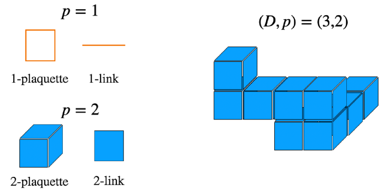
Figure 1: Left: $p$-plaquette and $p$-link in a cubic spacetime lattice. Here we show $p=1$ and $p=2$ cases.
Right: An example of discretized closed $2$-brane.

A fundamental issue in constructing a field theory of branes is how to express its kinetic term. A general variation of $\phi[C_{p}]$ under an arbitrary deformation of $p$-brane $\delta C_{p}=\{\delta X^{\mu}(\xi)\}_{\mu=0}^{D-1}$ is expressed by the conventional functional derivative as

$$\delta\phi[C_{p}]=\int_{S^{p}}d^{p}\xi~\delta X^{\mu}(\xi)\frac{\delta\phi[C_{p}]}{\delta X^{\mu}(\xi)}~.$$ (10)

See Appendix A for more details about the functional derivatives. Although this expression applies to an arbitrary deformation of a $p$-dimensional manifold, its geometric meaning is less clear except for $p=0$, where the functional derivative reduces to the ordinary derivative $\partial/\partial x^{\mu}$. In the following, we will show that the right-hand side in Eq. (10) can be also expressed in terms of geometrical functional derivative known as the area derivative when $\delta C_{p}$ is a genuinely $p$-dimensional deformation of $C_{p}$, i.e. when $C_{p}+\delta C_{p}$ preserves the topology of $C_{p}$. A physically intuitive and transparent way to introduce the area derivative is to consider a discretized spacetime and take the continuum-limit as follows.

Consider a $D$-dimensional cubic lattice $\Lambda_{D}$ with a lattice spacing $a$. In this discretized spacetime, a closed $p$-brane $C_{p}$ is expressed by gluing $p$-dimensional minimum hypercubes, as depicted in the right-panel in Fig. 1. (In this case, a $2$-dimensional surface $C_{2}$ is obtained by gluing many squares.) Following the same convention as lattice gauge theory, we call such a minimum $p$-dimensional hypercube $p$-link. Besides, a minimum closed $p$-brane is represented by the boundary of a $(p+1)$-link and we refer to it as $p$-plaquette. They are graphically shown in the left-panel in Fig.1. In particular, a $p$-plaquette existing in the $(p+1)$-dimensional subspace $(X^{\mu_{1}},\cdots,X^{\mu_{p+1}})$ is represented by $P^{\mu_{1}\cdots\mu_{p+1}}$. Moreover, we represent the center-of-mass of a given $p$-link as $\hat{i}$ below.

In this setup, an infinitesimal deformation of $C_{p}$ is represented by gluing a $p$-plaquette to one of the $p$-links on $C_{p}$ as illustrated in Fig. 2. This addition results in a new $p$-brane $C_{p}+P^{\mu_{1}\cdots\mu_{p+1}}(\hat{i})$, where $(\hat{i})$ implies that a $p$-plaquette is glued to the $p$-link whose center-of-mass position is $\hat{i}$. By construction, $C_{p}+P^{\mu_{1}\cdots\mu_{p+1}}(\hat{i})$ has the same topology as $C_{p}$. Now, we can define geometrical functional derivative via

$$\frac{\delta\phi[C_{p}]}{\delta\sigma^{\mu_{1}\cdots\mu_{p+1}}(\hat{i})}\coloneq\frac{\phi[C_{p}+P^{\mu_{1}\cdots\mu_{p+1}}(\hat{i})]-\phi[C_{p}]}{a^{p+1}}~,$$ (11)

which is known as the area derivative for $p=1$ [24, 25, 26, 27, 28, 19, 1, 2, 3]. In the following, we refer to Eq. (11) (and its continuum-limit) as the area derivative too for ${}^{\forall}p\geq 1$. It should be emphasized that this area derivative is defined only when the topology of $\delta C_{p}$ is the same as $S^{p}$ by construction. In this sense, the area derivative is a reduced functional derivative compared to $\delta/\delta X^{\mu}(\xi)$.

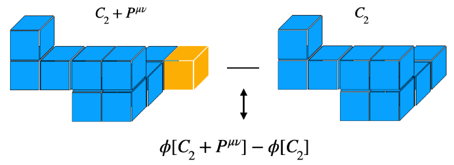
Figure 2: A graphical representation of the functional variation of the $2$-brane field $\phi[C_{2}]$ when adding a $2$-plaquette.

Equation (11) implies that the variation $\delta\phi[C_{p}]$ can be written as

$$\delta\phi[C_{p}] =\frac{1}{(p+1)!}\int_{\delta D_{p+1}}dX^{\mu_{1}}\wedge\cdots\wedge dX^{\mu_{p+1}}\frac{\delta\phi[C_{p}]}{\delta\sigma^{\mu_{1}\cdots\mu_{p+1}}(\xi)}$$ (12)

$$=\frac{1}{(p+1)!}\sigma^{\mu_{1}\cdots\mu_{p+1}}[\delta C_{p}(\xi)]\frac{\delta\phi[C_{p}]}{\delta\sigma^{\mu_{1}\cdots\mu_{p+1}}(\xi)}$$ (13)

in the continuum-limit, where $\delta C_{p}(\xi)$ is the infinitesimal closed manifold corresponding to $P^{\mu_{1}\cdots\mu_{p+1}}(\hat{i})$, and

$$\sigma^{\mu_{1}\cdots\mu_{p+1}}[C_{p}]=\int_{D_{p+1}}dX^{\mu_{1}}\wedge\cdots\wedge dX^{\mu_{p+1}}=\frac{1}{(p+1)!}\int_{C_{p}}X^{[\mu_{1}}(\xi)dX^{\mu_{2}}\wedge\cdots\wedge dX^{\mu_{p+1}]}~$$ (14)

is the area element of the $(p+1)$-dimensional open manifold $D_{p+1}$ surrounded by $C_{p}$. In the last equality, we have used the Stokes theorem and introduced the anti-symmetrization by

$$A^{[\mu_{1}\mu_{2}\cdots\mu_{p}]}\coloneq\sum_{\sigma\in S_{p}}\mathrm{sgn}(\sigma)A^{\sigma(\mu_{1})\sigma(\mu_{2})\cdots\sigma(\mu_{p})}~,$$ (15)

where $S_{p}$ is the symmetric group of degree $p$ and $\mathrm{sgn}(\sigma)$ is the sign of permutation. Intuitively, the area element (14) represents the surface area of the projected $p$-brane onto the $(X^{\mu_{1}},\cdots,X^{\mu_{p+1}})$ subspace. In Fig. 3, we show an example of $1$-brane.

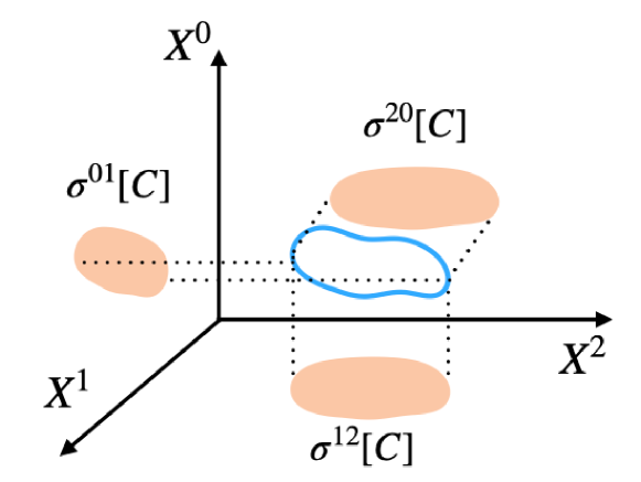
Figure 3: Area elements (orange) of a loop $C$ (blue).

Equation (12) must coincide with Eq. (10), which then provides a relation between $\delta/\delta X^{\mu}(\xi)$ and $\delta/\delta\sigma^{\mu_{1}\cdots\mu_{p+1}}(\xi)$ as [1]

$$\frac{\delta}{\delta X^{\mu}(\xi)}=\frac{1}{p!}\{X^{\nu_{1}},\cdots,X^{\nu_{p}}\}\frac{\delta}{\delta\sigma^{\mu\nu_{1}\cdots\nu_{p}}(\xi)}~$$ (16)

as long as $\delta C_{p}$ is a genuinely $p$-dimensional deformation of $C_{p}$. For more general deformations of $C_{p}$, this relation does not necessary hold and $\delta/\delta X^{\mu}(\xi)$ encompasses more functional information. In particular, the right-hand side in Eq. (16) depends only on the relative coordinates of $p$-brane defined by

$$Y^{\mu}(\xi)\coloneq X^{\mu}(\xi)-x^{\mu}_{\mathrm{CM}}~,$$ (17)

where

$$x_{\mathrm{CM}}^{\mu}\coloneq\frac{1}{\mathrm{Vol}[C_{p}]}\int_{S^{p}}d^{p}\xi\sqrt{h(\xi)}X^{\mu}(\xi)~$$ (18)

is the center-of-mass coordinate. Namely, the right-hand side in Eq. (16) cannot describe a variation of the brane-field $\phi[C_{p}]$ against the change of the center-of-mass position $x_{\mathrm{CM}}^{\mu}~\rightarrow~x_{\mathrm{CM}}^{\mu}+\delta x_{\mathrm{CM}}^{\mu}$. Thus, Eq. (16) is generalized as

$$\frac{\delta}{\delta X^{\mu}(\xi)}=\frac{\partial}{\partial x_{\mathrm{CM}}^{\mu}}+\frac{1}{p!}\{X^{\nu_{1}},\cdots,X^{\nu_{p}}\}\frac{\delta}{\delta\sigma^{\mu\nu_{1}\cdots\nu_{p}}(\xi)}+\cdots$$ (19)

for a general deformation $\delta C_{p}$. Here, $\cdots$ denotes other contributions that cannot be described by the first two terms.

What are the advantages of the area derivative ? The most important property is a differential property when acting on a volume integral of a differential $p$-form $A_{p}(X)$ as [1]

$$\frac{\delta}{\delta\sigma^{\mu_{1}\cdots\mu_{p+1}}(\xi)}\left(\int_{C_{p}}A_{p}\right)=F_{\mu_{1}\cdots\mu_{p+1}}(X(\xi))~,$$ (20)

where $F_{\mu_{1}\cdots\mu_{p+1}}(X)$ is the field strength defined by

$$F_{p+1}(X)=\frac{1}{(p+1)!}F_{\mu_{1}\cdots\mu_{p+1}}(X)dX^{\mu_{1}}\wedge\cdots\wedge dX^{\mu_{p+1}}\coloneq dA_{p}(X)~.$$ (21)

This property plays a crucial role in the following discussion. Besides, one can see that the area derivative of the $p$-brane volume is

$$\frac{\delta\mathrm{Vol}[C_{p}]}{\delta\sigma^{\mu_{1}\cdots\mu_{p+1}}(\xi)}=(dE_{p}(\xi))_{\mu_{1}\cdots\mu_{p+1}}$$ (22)

by Eq. (3). This implies that the volume derivative is included in the area derivative as

$$\frac{\delta}{\delta\sigma^{\mu_{1}\cdots\mu_{p+1}}(\xi)}=(dE_{p}(\xi))_{\mu_{1}\cdots\mu_{p+1}}\frac{\partial}{\partial\mathrm{Vol}[C_{p}]}~.$$ (23)

See also Refs. [24, 25, 19] for $p=1$ case.

2.2 Brane field action

Reflecting the fact that $p$-brane has a lot of dynamical degrees of freedom, we can consider a variety of kinetic terms such as

$$\int_{S^{p}}\frac{d^{p}\xi}{\sqrt{h(\xi)}}~\frac{\delta\phi^{*}[C_{p}]}{\delta X^{\mu}(\xi)}\frac{\delta\phi[C_{p}]}{\delta X_{\mu}(\xi)}~,\quad\int_{S^{p}}d^{p}\xi\sqrt{-h(\xi)}\frac{\delta\phi^{*}[C_{p}]}{\delta\sigma^{\mu_{1}\cdots\mu_{p+1}}(\xi)}\frac{\delta\phi[C_{p}]}{\delta\sigma_{\mu_{1}\cdots\mu_{p+1}}(\xi)}~,$$ (24)

$$\int_{S^{p}}\frac{d^{p}\xi}{\sqrt{h(\xi)}}\{X^{\nu_{1}},\cdots,X^{\nu_{p}}\}\{X^{\lambda_{1}},\cdots,X^{\lambda_{p}}\}\frac{\delta\phi^{*}[C_{p}]}{\delta\sigma^{\mu\nu_{1}\cdots\nu_{p}}(\xi)}\frac{\delta\phi[C_{p}]}{\delta{\sigma_{\mu}}^{\lambda_{1}\cdots\lambda_{p}}(\xi)}~.$$ (25)

As we mentioned in the previous section, the first one is the most general and encompasses all the functional information of $p$-brane. However, such a generality makes the analysis of the model quite challenging as in string field theory. In the previous studies [1, 2], we have performed the mean-field analysis by assuming the second kinetic term in Eq. (24) and found that it can consistently explain the various fundamental results associated with the spontaneous breaking of higher-form global symmetries. Note that the third one (25) also appears in the string field theory dual to the $\mathrm{SU}(N)$ gauge theory [3].

In this paper, as a generalization of our previous studies, we consider the following brane-field action:

$$S[\phi]=-{\cal N}\int[dC_{p}]\bigg{[}\frac{1}{\mathrm{Vol}[C_{p}]^{2}}\frac{\partial\phi^{*}[C_{p}]}{\partial x_{\mathrm{CM}}^{\mu}}\frac{\partial\phi[C_{p}]}{\partial x_{\mathrm{CM}\mu}} +\frac{1}{\mathrm{Vol}[C_{p}]}\int_{S^{p}}d^{p}\xi\sqrt{-h(\xi)}\frac{\delta\phi^{*}[C_{p}]}{\delta\sigma^{\mu_{1}\cdots\mu_{p+1}}(\xi)}\frac{\delta\phi[C_{p}]}{\delta\sigma_{\mu_{1}\cdots\mu_{p+1}}(\xi)}$$

$$+V(\phi[C_{p}],\phi^{*}[C_{p}])\bigg{]}~,$$ (26)

where $V(\phi[C_{p}],\phi^{*}[C_{p}])$ is a general potential, ${\cal N}$ is a normalization factor, and $[dC_{p}]$ is the (path)integral measure of $C_{p}$ induced by the diffeomorphism and reparametrization invariant norm

$$||\delta X||^{2}\coloneq\int_{S^{p}}d^{p}\xi\sqrt{-h(\xi)}\delta X^{\mu}(\xi)\delta X_{\mu}(\xi)~.$$ (27)

In particular, it contains the ordinary spacetime integral of the center-of-mass coordinates

$$\int_{\Sigma_{D}}\star 1\in\int[dC_{p}]~.$$ (28)

Taking this into account, we also express the measure as

$$\int[dC_{p}]=\int_{\Sigma_{D}}\star 1\int[dY]~,$$ (29)

where $[dY]$ denotes the path-integral measure of the relative coordinates. In Eq. (26), the geometrical meaning of the kinetic terms is quite manifest. The first term represents the center-of-mass motion of $p$-brane with the inertia factor of $1/\mathrm{Vol}[C_{p}]^{2}$, while the second term describes the motion of the area elements $\sigma^{\mu_{1}\cdots\mu_{p+1}}[C_{p}]$. Although the action (26) may not capture the full dynamics of $p$-brane, we will see that it describes the essential aspects of phase structures associated with higher-form global symmetries.

2.3 Global symmetries

Let us discuss global symmetries of the action (26). When the potential $V(\phi[C_{p}],\phi^{*}[C_{p}])$ is a mere function of $\phi^{*}[C_{p}]\phi[C_{p}]$, the action is invariant under the $\mathrm{U}(1)$ $p$-form global transformation

$$\phi[C_{p}]\quad\rightarrow\quad e^{i\int_{C_{p}}\Lambda_{p}}\phi[C_{p}]~,\quad d\Lambda_{p}=0~,$$ (30)

where $\Lambda_{p}$ is a differential closed (and non-exact) $p$-form. In fact, one can check that the kinetic term is invariant under Eq. (30) due to Eq. (20). Besides, the action is invariant under the $\mathrm{U}(1)$ $0$-form global transformation $\phi[C_{p}]\rightarrow e^{i\theta}\phi[C_{p}]$, corresponding to the conservation of total number of $p$-branes.

We can construct the conserved currents by the Nöther method [1]. Instead of Eq. (30), we consider a local $p$-form transformation:

$$\phi[C_{p}]\quad\rightarrow\quad e^{i\int_{C_{p}}\Lambda_{p}}\phi[C_{p}]~,\quad d\Lambda_{p}\neq 0~,$$ (31)

which leads to the variation of the action as

$$\delta S =-{\cal N}\int[dC_{p}]\frac{i}{\mathrm{Vol}[C_{p}](p+1)!}\int_{S^{p}}d^{p}\xi\sqrt{h(\xi)}\left(\frac{\delta\phi^{*}[C_{p}]}{\delta\sigma^{\mu_{1}\cdots\mu_{p+1}}(\xi)}\phi[C_{p}]-\phi^{*}[C_{p}]\frac{\delta\phi[C_{p}]}{\delta\sigma^{\mu_{1}\cdots\mu_{p+1}}(\xi)}\right)(d\Lambda_{p})_{\mu_{1}\cdots\mu_{p+1}}$$

$$=-\int_{\Sigma_{D}}d\Lambda_{p}\wedge\star J_{p+1}~,$$ (32)

where

$$J_{p+1}(X)={\cal N}\int[dC_{p}]\frac{i}{\mathrm{Vol}[C_{p}](p+1)!}\int_{S^{p}} d^{p}\xi\sqrt{h(\xi)}\left(\frac{\delta\phi^{*}[C_{p}]}{\delta\sigma^{\mu_{1}\cdots\mu_{p+1}}(\xi)}\phi[C_{p}]-\phi^{*}[C_{p}]\frac{\delta\phi[C_{p}]}{\delta\sigma^{\mu_{1}\cdots\mu_{p+1}}(\xi)}\right)$$

$$\times\frac{\delta^{(D)}(X-X(\xi))}{\sqrt{-g(X(\xi))}}dX^{\mu_{1}}\wedge\cdots\wedge dX^{\mu_{p+1}}~.$$ (33)

When $\phi[C_{p}]$ satisfies the equation of motion, the variation (32) vanishes and we obtain

$$d\star J_{p+1}(x_{\mathrm{CM}})=0~,$$ (34)

which represents the conservation law of the $\mathrm{U}(1)$ $p$-form global symmetry. Similarly, we can consider a local $\mathrm{U}(1)$ $0$-form local transformation $\phi[C_{p}]\rightarrow e^{i\theta(x_{\mathrm{CM}})}\phi[C_{p}]$ and obtain

$$J_{1}(x_{\mathrm{CM}})={\cal N} \int[dY]\frac{i}{\mathrm{Vol}[C_{p}]^{2}}\left(\frac{\partial\phi^{*}[C_{p}]}{\partial x_{\mathrm{CM}}^{\mu}}\phi[C_{p}]-\phi^{*}[C_{p}]\frac{\partial\phi[C_{p}]}{\partial x_{\mathrm{CM}}^{\mu}}\right)dx_{\mathrm{CM}}^{\mu}~,$$ (35)

which reproduces the ordinary particle current

$$i(\partial_{\mu}\phi^{*}(x_{\mathrm{CM}})\phi(x_{\mathrm{CM}})-\phi^{*}(x_{\mathrm{CM}})\partial_{\mu}\phi(x_{\mathrm{CM}}))dx_{\mathrm{CM}}^{\mu}$$ (36)

when $p=0$.

If the potential $V(\phi[C_{p}],\phi^{*}[C_{p}])$ contains terms such as $g\phi[C_{p}]^{N}+\mathrm{h.c.}$, these $\mathrm{U}(1)$ global symmetries are explicitly broken down to $\mathbb{Z}_{N}$ symmetries given by

$$\phi[C_{p}]\quad \rightarrow\quad e^{\frac{i}{N}\int_{C_{p}}\Lambda_{p}}\phi[C_{p}]\quad\text{with}\quad d\Lambda_{p}=0~,\quad\int_{C_{p}}\Lambda_{p}\in 2\pi\mathbb{Z}~,$$ (37)

$$\phi[C_{p}]\quad \rightarrow\quad e^{\frac{2\pi i}{N}n}\phi[C_{p}]~,\quad n\in\mathbb{Z}~.$$ (38)

In this case, the system is gapped after the spontaneous symmetry breaking and exhibits topological order as we will see below.

2.4 Mean-field analysis

Here, we perform the mean-field analysis of the theory (26). Since many parts of the calculations overlap with our previous studies [1, 2, 19], we will focus on highlighting the main results and differences compared to these previous studies.

As in ordinary QFT, the center-of-mass kinetic term does not play a crucial role when investigating the vacuum state, which then leads to the following equation of motion of the brane-field:

$$\frac{1}{(p+1)!}\int_{S^{p}}d^{p}\xi\frac{\delta}{\delta\sigma^{\mu_{1}\cdots\mu_{p+1}}(\xi)}\frac{\sqrt{h(\xi)}}{\mathrm{Vol}[C_{p}]}\frac{\delta\phi[C_{p}]}{\delta\sigma_{\mu_{1}\cdots\mu_{p+1}}(\xi)}-\frac{\delta V(\phi[C_{p}],\phi^{*}[C_{p}])}{\delta\phi^{*}[C_{p}]}=0~.$$ (39)

UNBROKEN PHASE
Let us consider the unbroken phase of the global symmetries, i.e. we focus on the parameter space such that the potential $V(\phi[C_{p}],\phi^{*}[C_{p})$ has an absolute minimum at $\phi[C_{p}]=0$. In this case, Eq. (39) admits a solution that exhibits the area law in the large-volume limit, $\mathrm{Vol}[C_{p}]\rightarrow\infty$ [1, 2, 3, 19]. In fact, we consider the following ansatz

$$\phi[C_{p}]=\frac{1}{\sqrt{2}}f(\mathrm{Vol}[M_{p+1}])~,$$ (40)

where $f(z)$ is an arbitrary real function and $M_{p+1}$ is the $(p+1)$-dimensional minimal surface enclosed by $C_{p}$, i.e. $\partial M_{p+1}=C_{p}$. Analogously to Eq. (2), we represent the minimum-surface volume as

$$\mathrm{Vol}[M_{p+1}]=\int_{M_{p+1}}E_{p}=\frac{1}{(p+1)!}\int_{M_{p+1}}(E_{p+1})_{\mu_{1}\cdots\mu_{p+1}}dX^{\mu_{1}}\wedge\cdots\wedge dX^{\mu_{p+1}}~.$$ (41)

Putting the above ansatz into Eq. (39), we obtain the effective equation of motion:

$$f^{\prime\prime}(z)-q(z)f^{\prime}(z)-\frac{\delta V(f)}{\delta f(z)}=0~,\quad z=\mathrm{Vol}[M_{p+1}]~,$$ (42)

where

$$q(z)=\frac{1}{(p+1)!}\int_{S^{p}}d^{p}\xi\frac{\delta}{\delta\sigma^{\mu_{1}\cdots\mu_{p+1}}(\xi)}\left(\frac{\sqrt{h(\xi)}}{\mathrm{Vol}[C_{p}]}E^{\mu_{1}\cdots\mu_{p+1}}(\xi)\right)~,$$ (43)

which is dependent only on the geometrical information of $C_{p}$ and does not depend on the parameters of $V(\phi[C_{p}],\phi^{*}[C_{p}])$. Thus, it should behave as $q(z)\propto z^{-1}$ for $z\rightarrow\infty$ on dimensional ground and Eq. (42) can be approximated as

$$f^{\prime\prime}(z)-T_{p}^{2}f(z)\approx 0$$ (44)

for $z\rightarrow\infty$, where we have expanded the potential around $\phi[C_{p}]=0$ as $V(\phi[C_{p}],\phi^{*}[C_{p}])\approx T_{p}^{2}\phi[C_{p}]\phi^{*}[C_{p}]$. Equation (44) corresponds to the area law solution

$$\phi[C_{p}]\approx\frac{1}{\sqrt{2}}\exp\left(-T_{p}\times\mathrm{Vol}[M_{p+1}]\right)\quad\text{for }z\rightarrow\infty~,$$ (45)

which is a characteristic behavior of the unbroken phase of higher-form symmetries. One can see that $T_{p}$ corresponds to the $p$-brane tension.

BROKEN PHASE
The global symmetries are spontaneously broken when the brane-field develops a nonzero VEV, $\langle\phi[C_{p}]\rangle=v/\sqrt{2}\neq 0$. The Nambu-Goldstone modes are given by the phase modulations defined by

$$\phi[C_{p}]=\frac{v}{\sqrt{2}}\exp\left(i\varphi(x_{\mathrm{CM}})+i\int_{C_{p}}A_{p}\right)~,$$ (46)

where $\varphi(x_{\mathrm{CM}})$ is a compact real scalar field satisfying $\varphi(x_{\mathrm{CM}})\sim\varphi(x_{\mathrm{CM}})+2\pi$, and $A_{p}$ is a $p$-form field. From the point of view of these phase modulations, the original global transformations correspond to

$$\varphi\quad \rightarrow\quad\varphi+\theta~,\quad\theta\in\mathbb{R}~,$$ (47)

$$A_{p}\quad \rightarrow\quad A_{p}+\Lambda_{p}~,\quad d\Lambda_{p}=0~,$$ (48)

and the low-energy effective theory must be invariant under these transformations. In fact, we can explicitly calculate it as [1, 2]

$$S_{\mathrm{eff}}[\varphi,A_{p}]=-\frac{v^{2}}{2}\int_{\Sigma_{D}}\left[d\varphi\wedge\star d\varphi+F_{p+1}\wedge\star F_{p+1}\right]~,$$ (49)

where $F_{p+1}=dA_{p}$ is the field strength of $A_{p}$ and $\star$ is the Hodge dual operator. The first term is the ordinary kinetic term of the NG mode $\varphi$, whereas the second term corresponds to the $p$-form Maxwell theory.

Equation (49) has emergent (magnetic) higher-form symmetries represented by

$$dd\varphi=0~,\quad dF_{p+1}=0~,$$ (50)

which correspond to $\mathrm{U}(1)$ $(D-2)$- and $(D-p-2)$-form global symmetries respectively. The corresponding charges are

$$Q_{D-2} =\frac{1}{2\pi}\int_{C_{1}}d\varphi\quad\in\mathbb{Z}~,\quad Q_{D-p-2}=\frac{1}{2\pi}\int_{C_{p+1}}F_{p+1}\quad\in\mathbb{Z}~.$$ (51)

These emergent higher-form symmetries indicate the existence of $(D-2)$- and $(D-p-2)$-dimensional topological defects in spacetime. The former is nothing but the well-known global vortex configuration and the latter corresponds to a topologically non-trivial $(D-p-3)$-dimensional static configuration characterized by the winding number of $C_{p}\sim S^{p}$ on $S^{p+1}$ for a given time slice [36].

DISCRETE SYMMETRIES AND TOPOLOGICAL ORDER
When the $\mathrm{U}(1)$ global symmetries are explicitly broken down to $\mathbb{Z}_{N}$ by the explicit breaking terms such as $\phi[C_{p}]^{N}$, the system is no longer gapless in the broken phase and exhibits topological order. By repeating the same calculations as Refs. [1, 2], the low-energy effective action in the presence of the $\phi[C_{p}]^{N}$ potential term is given as

$$S_{\mathrm{eff}}=\frac{N}{2\pi}\int_{\Sigma_{D}}H_{D-1}\wedge d\varphi +\frac{N}{2\pi}\int_{\Sigma_{D}}B_{D-p-1}\wedge dA_{p}~,$$ (52)

where $H_{D-1}(X)$ and $B_{D-p-1}(X)$ are $(D-1)$- and $(D-p-1)$-form fields. This is a $\mathrm{BF}$-type topological field theory and exhibits topological order. In addition to the original $\mathbb{Z}_{N}$ $0$- and $p$-form symmetries (47)(48), Eq. (52) has emergent $\mathbb{Z}_{N}$ $(D-1)$- and $(D-p-1)$-form symmetries expressed by

$$H_{D-1}\quad \rightarrow\quad H_{D-1}+\frac{1}{N}\Lambda_{D-1}~,\quad d\Lambda_{D-1}=0~,\quad\int_{C_{D-1}}\Lambda_{D-1}\in 2\pi\mathbb{Z}~,$$ (53)

$$B_{D-p-1}\quad \rightarrow\quad B_{D-p-1}+\frac{1}{N}\Lambda_{D-p-1}~,\quad d\Lambda_{D-p-1}=0~,\quad\int_{C_{D-p-1}}\Lambda_{D-p-1}\in 2\pi\mathbb{Z}~,$$ (54)

where $C_{D-1}$ ($C_{D-p-1}$) is a $(D-1)~((D-p-1))$-dimensional closed subspace. Namely, Eq. (52) has totally four topological operators:

$$U_{0}(C_{D-1}) =\exp\left(i\int_{C_{D-1}}H_{D-1}\right)~,\quad U_{p}(C_{D-p-1})=\exp\left(i\int_{C_{D-p-1}}B_{D-p-1}\right)~,$$ (55)

$$U_{D-1}(P,P^{\prime}) =\exp\left(i(\varphi(P)-\varphi(P^{\prime}))\right)~,\quad U_{D-p-1}(C_{p})=\exp\left(i\int_{C_{p}}A_{p}\right)~,$$ (56)

where $P$ and $P^{\prime}$ denote spacetime points. When the spatial manifold is flat, i.e. $\Sigma_{D-1}=\mathbb{R}^{D-1}$, all the topological operators (except for $U_{D-1}(P,P^{\prime})$) can trivially shrink to a point, which then implies $\langle U_{0}(C_{D-1})\rangle=\langle U_{p}(C_{D-p-1})\rangle=\langle U_{D-p-1}(C_{p})\rangle=1$. Since they also correspond to the charged objects under these higher-form symmetries, this means that these symmetries are spontaneously broken.

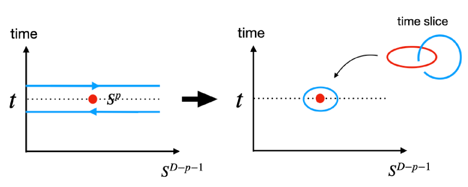
Figure 4: Graphical representation of the operator relation (57).

On the other hand, when the topology of spatial manifold is nontrivial, these topological operators can act nontrivially on the ground states. As an example, let us consider $\Sigma_{D-1}=S^{p}\times S^{D-p-1}$ and choose $C_{p}=S^{p}$ and $C_{D-p-1}=S^{D-p-1}$. In this case, two symmetry operators $U_{p}(S^{D-p-1})$ and $U_{D-p-1}(S^{p})$ are linked and satisfies

$$U_{p}(S^{D-p-1})U_{D-p-1}(S^{p})U_{p}^{-1}(S^{D-p-1})=e^{i\frac{2\pi}{N}}U_{D-p-1}(S^{p})$$ (57)

as an equal-time operator relation. In Fig. 4, we show the graphical representation of this relation. Then, when we choose a ground state $|\Omega\rangle$ as an simultaneous eigenstate of $U_{p}(S^{D-p-1})$ as

$$U_{p}(S^{D-p-1})|\Omega\rangle=e^{i\theta}|\Omega\rangle~,\quad\theta\in\mathbb{R}~,$$ (58)

$|\Omega^{\prime}\rangle\coloneq U_{D-p-1}(S^{p})|\Omega\rangle$ also has the same energy as $|\Omega\rangle$ because $U_{D-p-1}(S^{p})$ is a symmetry operator. However, it has a different eigenvalue of $U_{p}(S^{D-p-1})$ as

$$U_{p}(S^{D-p-1})|\Omega^{\prime}\rangle=e^{i\theta+i\frac{2\pi}{N}}|\Omega^{\prime}\rangle$$ (59)

due to the commutation relation (57), which implies that $|\Omega^{\prime}\rangle$ is another degenerate ground state. By repeating the same calculations, one can see that there are $N$-degenerate states in this case.

2.5 More on phases of higher-form symmetries

So far, we have considered brane-field theories with simple contact interactions. The present effective framework, however, also allows a variety of interactions that can lead to diverse (quantum) phases of branes in the low-energy limit. For example, we can consider non-local interactions such as [22, 19]

$$\int[dC_{p}^{(1)}]\int[dC_{p}^{(2)}]\int[dC_{p}^{(3)}]\delta(C_{p}^{(1)}+C_{p}^{(2)}+C_{p}^{(3)})\phi[C_{p}^{(1)}]\phi[C_{p}^{(2)}]\phi[C_{p}^{(3)}]+\mathrm{h.c.}~,$$ (60)

where $\delta(C_{p}^{(1)}+C_{p}^{(2)}+C_{p}^{(3)})$ is a delta function in the $p$-brane space that restricts the path-integral configurations to $C_{p}^{(1)}=-C_{p}^{(2)}-C_{p}^{(3)}$. This interaction preserves the $\mathrm{U}(1)$ $p$-form global symmetry as

$$\delta(C_{p}^{(1)}+C_{p}^{(2)}+C_{p}^{(3)})\phi[C_{p}^{(1)}]\phi[C_{p}^{(2)}]\phi[C_{p}^{(3)}]$$

$$\rightarrow\quad \delta(C_{p}^{(1)}+C_{p}^{(2)}+C_{p}^{(3)})e^{i\int_{C_{p}^{(1)}+C_{p}^{(2)}+C_{p}^{(3)}}\Lambda_{p}}\phi[C_{p}^{(1)}]\phi[C_{p}^{(2)}]\phi[C_{p}^{(3)}]$$

$$=\delta(C_{p}^{(1)}+C_{p}^{(2)}+C_{p}^{(3)})\phi[C_{p}^{(1)}]\phi[C_{p}^{(2)}]\phi[C_{p}^{(3)}]~,$$ (61)

while it explicitly breaks the $\mathrm{U}(1)$ $0$-form global symmetry down to $\mathbb{Z}_{3}$. In this case, the $p$-form phase modulation $A_{p}$ remains gapless after the symmetry breaking, whereas the axion field $\varphi(x_{\mathrm{CM}})$ is gapped as we have seen in the previous sections.

Furthermore, we can consider the higher area-derivative terms such as

$$i\lambda\int[dC_{p}]\frac{1}{\mathrm{Vol}[C_{p}]}\int_{S^{p}}d^{p}\xi\sqrt{h(\xi)}~D_{p+1}\phi[C_{p}]\wedge\cdots\wedge D_{p+1}\phi[C_{p}]+\mathrm{h.c.}~,$$ (62)

for $D=(p+1)M~,~M\in\mathbb{Z}$, where $\lambda\in\mathbb{R}$ is a coupling constant and

$$D_{p+1}\phi[C_{p}]\coloneq\frac{1}{(p+1)!}\frac{\delta\phi[C_{p}]}{\delta\sigma^{\mu_{1}\cdots\mu_{p+1}}(\xi)}dX^{\mu_{1}}\wedge\cdots\wedge dX^{\mu_{p+1}}~.$$ (63)

Equation (62) explicitly breaks the $\mathrm{U}(1)$ global symmetries down to $\mathbb{Z}_{M}$ and results in the following low-energy effective term in the broken phase:

$$\lambda\int_{\Sigma_{D}}\sin\left(M\varphi\right)F_{p+1}\wedge\cdots\wedge F_{p+1}~,$$ (64)

where we have neglected the higher-dimensional terms of $A_{p}$ for simplicity. Thus, when the potential $V(\phi[C_{p}],\phi^{*}[C_{p}])$ explicitly breaks the $\mathrm{U}(1)$ global symmetries down to $\mathbb{Z}_{N}$, the full low-energy effective action becomes

$$S_{\mathrm{eff}}\approx\frac{N}{2\pi}\int_{\Sigma_{D}}H_{D-1}\wedge d\varphi+\frac{N}{2\pi}\int_{\Sigma_{D}}B_{D-p-1}\wedge dA_{p}+\lambda\int_{\Sigma_{D}}\sin\left(M\varphi\right)F_{p+1}\wedge\cdots\wedge F_{p+1}~.$$ (65)

This is a similar effective action to the topological axion electrodynamics [29, 30]. In the present model, the remaining global symmetries are four higher-form symmetries described by the following equations of motion:

• $\mathbb{Z}_{q}$ $0$-form symmetry: $\frac{N(-1)^{D}}{2\pi}dH_{D-1}+\lambda M\cos(M\varphi)F_{p+1}\wedge\cdots\wedge F_{p+1}=0$

• $\mathbb{Z}_{q}$ $p$-form symmetry: $\frac{N(-1)^{D-p-1}}{2\pi}dB_{D-p-1}+\lambda d\sin(M\varphi)\wedge F_{p+1}\wedge\cdots\wedge F_{p+1}=0$

• $\mathbb{Z}_{N}$ $(D-p-1)$-form symmetry: $dA_{p}=0$

• $\mathbb{Z}_{N}$ $(D-1)$-form symmetry: $d\varphi=0$ ,

where $q$ is the greatest common divisor between $N$ and $M$. Each equations of motion can be interpreted as a topological conservation law $d\star J_{n+1}=0$, giving a topological charge $Q_{n}\coloneq\int_{C_{D-n-1}}\star J_{n+1}$ where $C_{D-n-1}$ is a $(D-n-1)$-dimensional subspace. As discussed in Ref. [29, 30], this theory exhibits the topological order on the axionic domain wall by the intersections of $0$- and $p$-form symmetry generators, in addition to the bulk topological order discussed in the previous section, Besides, these four higher-form symmetries give rise to the structure of higher-group symmetry where the correlations (or intersections) between symmetry operators satisfy nontrivial relations as quantum operators.

GAUGING HIGHER-FORM GLOBAL SYMMETRIES
It is also possible to gauge the higher-form global symmetries [1, 2]. The gauged version of Eq. (26) in a differential form is

$$S_{\text{gauged}}= -{\cal N}\int[dC_{p}]\bigg{[}\frac{1}{\mathrm{Vol}[C_{p}]^{2}}(D_{\mathrm{CM}}\phi[C_{p}])^{*}\wedge\star D_{\mathrm{CM}}\phi[C_{p}]$$

$$+\frac{1}{\mathrm{Vol}[C_{p}]}\int_{S^{p}}d^{p}\xi\sqrt{-h(\xi)}(D_{\sigma}\phi[C_{p}])^{*}\wedge\star D_{\sigma}\phi[C_{p}]+V(\phi[C_{p}]\phi^{*}[C_{p}])\bigg{]}$$

$$-\frac{1}{2g^{2}}\int_{\Sigma_{D}}F_{2}\wedge\star F_{2}-\frac{1}{2\tilde{g}^{2}}\int_{\Sigma_{D}}F_{p+2}\wedge\star F_{p+2}~,$$ (66)

where $g^{2}$ and $\tilde{g}^{2}$ are the gauge couplings and

$$D_{\mathrm{CM}}\phi[C_{p}] =(d-iq_{0}A_{1}(x_{\mathrm{CM}}))\phi[C_{p}]~,$$ (67)

$$D_{\sigma}\phi[C_{p}] =\frac{1}{(p+1)!}\left(\frac{\delta}{\delta\sigma^{\mu_{1}\cdots\mu_{p+1}}(\xi)}-iq_{p}A_{\mu_{1}\cdots\mu_{p+1}}(X(\xi))\right)\phi[C_{p}]dX^{\mu_{1}}\wedge\cdots\wedge dX^{\mu_{p+1}}~,$$ (68)

$$F_{2}=dA_{1}~,\quad F_{p+2}=dA_{p+1}~$$ (69)

with $q_{0},q_{p}\in\mathbb{Z}$. The gauge transformations are given by

$$\phi[C_{p}]\quad\rightarrow\quad e^{iq_{0}\Lambda(x_{\mathrm{CM}})}\phi[C_{p}]~,\quad A_{1}(x_{\mathrm{CM}})\quad\rightarrow\quad A_{1}(x_{\mathrm{CM}})+d\Lambda(x_{\mathrm{CM}})~,$$ (70)

$$\phi[C_{p}]\quad\rightarrow\quad e^{iq_{p}\int_{C_{p}}\Lambda_{p}}\phi[C_{p}]~,\quad A_{p+1}(X)\quad\rightarrow\quad A_{p+1}(X)+d\Lambda_{p}(X)~,$$ (71)

where $\Lambda(x_{\mathrm{CM}})$ ($\Lambda_{p}(X)$) is a differential $0~(p)$-form. The equations of motion of the gauge fields are

$$\frac{1}{g^{2}}d\star F_{2} =q_{0}\star J_{1}~,\quad\frac{(-1)^{p}}{\tilde{g}^{2}}d\star F_{p+2}=q_{p}\star J_{p+1}~,$$ (72)

by which we obtain the on-shell conservation laws, $d\star J_{1}=0~,~d\star J_{p+1}=0$. The corresponding conserved charges are

$$Q_{0} =\int_{\Sigma_{D-1}}\star J_{1}=\frac{1}{g^{2}q_{0}}\int_{C_{D-2}}\star F_{2}\in\mathbb{Z}~,$$ (73)

$$Q_{p} =\int_{\Sigma_{D-p-1}}\star J_{p+1}=\frac{1}{\tilde{g}^{2}q_{p}}\int_{C_{D-p-2}}\star F_{p+2}\in\mathbb{Z}~,$$ (74)

where $\Sigma_{D-1}$ ($\Sigma_{D-p-1}$) is an $(D-1)$ ($(D-p-1)$)-dimensional open subspace with a closed boundary $\partial\Sigma_{D-1}=C_{D-2}$ ($\partial\Sigma_{D-p-1}=C_{D-p-2}$). These conserved charges mean the existence of the electric $\mathbb{Z}_{q_{0}}$ $1$-form and $\mathbb{Z}_{q_{p}}$ $(p+1)$-form global symmetries, whose transformations are given by

$$A_{1} \quad\rightarrow\quad A_{1}+\frac{1}{q_{0}}\Lambda_{1}~,\quad d\Lambda_{1}=0~,\quad\int_{C_{1}}\Lambda_{1}\in 2\pi\mathbb{Z}~,$$ (75)

$$A_{p+1} \quad\rightarrow\quad A_{p+1}+\frac{1}{q_{p}}\Lambda_{p+1}~,\quad d\Lambda_{p+1}=0~,\quad\int_{C_{p+1}}\Lambda_{p+1}\in 2\pi\mathbb{Z}~,$$ (76)

where $C_{1}$ ($C_{p+1}$) is a $1$ ($(p+1)$)-dimensional closed subspace. In addition, the theory has the magnetic $\mathrm{U}(1)$ $(D-3)$- and $(D-p-3)$-form global symmetries described by

$$dF_{2}=0~,\quad dF_{p+2}=0~.$$ (77)

In the coulomb phase, the brane-field exhibits the area law $\langle\phi[C_{p}]\rangle\sim\exp(-T_{p}\mathrm{Vol}[M_{p+1}])$ as shown in the previous section, and the low-energy effective theory is simply described by the Maxwell theories of two gauge fields $A_{1}$ and $A_{p+1}$. These gapless modes can be interpreted as the Nambu-Goldstone modes of the broken magnetic higher-form symmetries (77) [2].

In the superconducting (Higgs) phase, i.e. $\langle\phi[C_{p}]\rangle=v/\sqrt{2}\neq 0$, on the other hand, the gauge fields become massive and the low-energy effective theory is described by a $\mathrm{BF}$-type topological field theory [1, 2]. Here, we present the essence of the derivation based on the symmetry argument. See Refs. [1, 2] for the detailed derivation. By introducing the phase fluctuations as Eq. (46), one can check that the classical currents (33)(35) become

$$J_{1}(x)\propto v^{2}d\varphi(x)~,\quad J_{p+1}(x)\propto v^{2}dA_{p}(x)~,$$ (78)

which satisfies $dJ_{1}=dJ_{p+1}=0$, representing the emergent $\mathbb{Z}_{q_{0}}$ $(D-2)$- and $\mathbb{Z}_{q_{p}}$ $(D-p-2)$-form global symmetries in the superconducting phase. The corresponding charged objects are the $(D-2)$ $((D-p-2))$-dimensional topological defect which can be analytically constructed in the present theory [2]. The low-energy effective theory must respect these global symmetries as well as the original symmetries (75)(76) and is gapped. Then, one can easily guess that the effective theory with these requirements is

$$S_{\mathrm{eff}}=\frac{q_{0}}{2\pi}\int_{\Sigma_{D}}B_{D-2}\wedge dA_{1}+\frac{q_{p}}{2\pi}\int_{\Sigma_{D}}B_{D-p-2}\wedge dA_{p+1}~,$$ (79)

where $B_{D-2}(X)$ ($B_{D-p-2}(X)$) is the dual field of $\varphi(X)$ ($A_{p}(X)$). This is a $\mathrm{BF}$-type topological field theory and exhibits topological order as explained in the previous section.

In this way, our brane-field theory provides an effective framework for describing a variety of (topological) phases of matter and can be regarded as a natural generalization of conventional Landau field theory for $0$-form symmetries to higher-form symmetries.

3 Propagation of $p$-brane

In this section, we study the propagation of $p$-brane in the brane-field theory. We will derive a path-integral expression of the brane propagator in the Schwinger’s proper time formalism and obtain approximate analytic expressions of the brane propagator in the Born-Oppenheimer approximation. We also discuss the Hausdorff dimension of $p$-brane within the approximation.

3.1 Plane wave and propagator

In the following, we consider the free theory, i.e.

$$V(\phi[C_{p}],\phi^{*}[C_{p}])=T_{p}^{2}\phi^{*}[C_{p}]\phi[C_{p}]~,$$ (80)

where $T_{p}$ corresponds to the $p$-brane tension with a mass dimension $p+1$. The time-ordered propagator is formally defined by

$$G[C_{p},C_{p}^{\prime}]=\langle T\{\phi[C_{p}]\phi^{\dagger}[C_{p}^{{}^{\prime}}]\}\rangle\coloneqq\frac{1}{Z}\int{\cal D}\phi^{*}{\cal D}\phi~\phi[C_{p}]\phi^{*}[C_{p}^{{}^{\prime}}]e^{iS[\phi]}~,$$ (81)

which can be written in the operator form as

$$=-\frac{i}{2}\langle C_{p}|\left(\hat{H}-i\varepsilon/2\right)^{-1}|C_{p}^{{}^{\prime}}\rangle=\frac{1}{2}\int_{0}^{\infty}dA\langle C_{p}|e^{-i(\hat{H}-i\frac{\varepsilon}{2})A}|C_{p}^{{}^{\prime}}\rangle~,$$ (82)

where $i\varepsilon$ is the Feynman’s prescription and

$$\hat{H} =\frac{1}{2}\left[-\frac{1}{\mathrm{Vol}[C_{p}]^{2}}\frac{\partial^{2}}{\partial x_{\mathrm{CM}}^{\mu}\partial x_{\mathrm{CM}\mu}}-\int_{S^{p}}d^{p}\xi~\frac{\delta}{\delta\sigma^{\mu_{1}\cdots\mu_{p+1}}(\xi)}\frac{\sqrt{h(\xi)}}{\mathrm{Vol}[C_{p}]}\frac{\delta}{\delta\sigma_{\mu_{1}\cdots\mu_{p+1}}(\xi)}+T_{p}^{2}\right]$$ (83)

is the Hamiltonian on the world-manifold. Note that $AT_{p}$ is interpreted as the proper surface-area of the $(p+1)$-dimensional world-manifold.

In order to calculate the above amplitude, we have to find the plane-wave solutions. As for the center-of-mass motion, it is well-known as

$$\langle x_{\mathrm{CM}}|k_{\mathrm{CM}}\rangle=\frac{1}{(2\pi)^{D/2}}e^{ik_{\mathrm{CM}}\cdot x_{\mathrm{CM}}}~.$$ (84)

We can similarly find the plane-wave for the area derivative as

$$\exp\left(i\int_{C_{p}}K_{p}\right)\coloneqq\exp\left(\frac{i}{(p+1)!}\int_{C_{p}}K_{\mu_{1}\cdots\mu_{p+1}}(\xi)Y^{[\mu_{1}}(\xi)dY^{\mu_{2}}\wedge\cdots\wedge dY^{\mu_{p+1}]}\right)~,$$ (85)

where $K_{\mu_{1}\cdots\mu_{p+1}}(\xi)$ is a real anti-symmetric function and we have explicitly used the relative coordinates $\{Y^{\mu}(\xi)\}$ in order to show that it is independent of $\{x_{\mathrm{CM}}^{\mu}\}$. Acting the area derivative, we can explicitly check that

$$-i\frac{\delta}{\delta\sigma^{\mu_{1}\cdots\mu_{p+1}}(\xi)}\exp\left(i\int_{C_{p}}K_{p}\right) =(dK_{p})_{\mu_{1}\cdots\mu_{p+1}}(\xi)\exp\left(i\int_{C_{p}}K_{p}\right)$$

$$=K_{\mu_{1}\cdots\mu_{p+1}}(\xi)\exp\left(i\int_{C_{p}}K_{p}\right)$$ (86)

by Eq. (20). In particular, the plane-wave of the volume dynamics can be identified by

$$(K_{p}^{\mathrm{Vol}})_{\mu_{1}\cdots\mu_{p+1}}\coloneq-(dE_{p}(\xi))_{\mu_{1}\cdots\mu_{p+1}}\times k_{\mathrm{Vol}}~,\quad k_{\mathrm{Vol}}\in\mathbb{R}~$$ (87)

due to Eq. (23). In fact, by putting this into Eq. (85), one can check

$$e^{i\int_{C_{p}}K_{p}^{\mathrm{Vol}}}=e^{ik_{\mathrm{Vol}}\mathrm{Vol}[C_{p}]}~$$ (88)

with the use of the Stokes theorem. In the following, we redefine $K_{p}-K_{p}^{\mathrm{Vol}}$ as $K_{p}$, which satisfies

$$K_{p}\cdot dE_{p}\coloneq\frac{1}{(p+1)!}K_{\mu_{1}\cdots\mu_{p+1}}(dE_{p})^{\mu_{1}\cdots\mu_{p+1}}=0~.$$ (89)

Namely, $K_{p}$ corresponds to the eigenmode of the shape deformation of $p$-brane. Then, the completeness relation is given by

$$1=\int\frac{d^{D}k_{\mathrm{CM}}}{(2\pi)^{D}}\int\frac{dk_{\mathrm{Vol}}}{2\pi}\int[dK_{p}]\bigg{(}|k_{\mathrm{CM}}\rangle\otimes|k_{\mathrm{Vol}}\rangle\otimes|K_{p}\rangle\bigg{)}\bigg{(}\langle K_{p}|\otimes\langle k_{\mathrm{Vol}}|\otimes\langle k_{\mathrm{CM}}|\bigg{)}~,$$ (90)

with an appropriate normalization, where the (path)integral measure $[dK_{p}]$ is chosen in the same manner as $[dC_{p}]$. Note that, although $|k_{\mathrm{CM}}\rangle\otimes|k_{\mathrm{Vol}}\rangle\otimes|K_{p}\rangle$ is the eigenstate of the center-of-mass and area derivatives, it is not an eigenstate of the Hamiltonian $\hat{H}$ due to the explicit $\{X^{\mu}(\xi)\}$ dependence via $h(\xi)$ and $\mathrm{Vol}[C_{p}]$ in Eq. (83). By repeatedly inserting the completeness relations into Eq. (82), we obtain the path-integral expression of the transition amplitude as

$$\langle C_{p}|e^{-i(\hat{H}-i\varepsilon)A}|C_{p}^{{}^{\prime}}\rangle=\int_{t=0,C^{\prime}_{p}}^{t=A,C_{p}}{\cal D}X\int{\cal D}k_{\mathrm{CM}}\int{\cal D}k_{\mathrm{Vol}}\int{\cal D}Ke^{iS_{p}}~,$$ (91)

where

$$S_{p} =\int_{0}^{A}dt\bigg{(}k_{\mathrm{CM}\mu}(t)\dot{x}_{\mathrm{CM}}^{\mu}(t)+k_{\mathrm{Vol}}(t)\dot{\mathrm{Vol}}[C_{p}(t)]-(H(t)-i\varepsilon)\bigg{)}+\int_{M_{p+1}}K_{p+1}$$ (92)

is the first quantized $p$-brane action. The following are the definitions of all the quantities appearing in Eq. (92):

$$H(t) =\frac{1}{2}\left(\frac{k^{2}}{\mathrm{Vol}[C_{p}(t)]^{2}}+D[C_{p}(t)]k_{\mathrm{Vol}}(t)^{2}+K_{p}(t)^{2}+T_{p}^{2}\right)~,$$ (93)

$$D[C_{p}(t)] =\frac{1}{\mathrm{Vol}[C_{p}(t)]}\int_{S^{p}}d^{p}\xi\sqrt{h(t,\xi)}(dE_{p})\cdot(dE_{p})$$ (94)

$$K_{p}(t)^{2} =\frac{1}{\mathrm{Vol}[C_{p}(t)]}\int_{S^{p}}d^{p}\xi\sqrt{h(t,\xi)}K_{p}\cdot K_{p}~,$$ (95)

$$\int_{M_{p+1}}K_{p+1} =\frac{1}{(p+1)!}\int_{M_{p+1}}K_{\mu_{1}\cdots\mu_{p+1}}(t,\xi)dY^{\mu_{1}}\wedge\cdots\wedge dY^{\mu_{p+1}}~,$$ (96)

where the product $A\cdot B$ is similarly defined by Eq. (89) and $M_{p+1}$ is the $(p+1)$-dimensional world-manifold of $p$-brane with boundaries $\partial M_{p+1}=C_{p}-C_{p}^{{}^{\prime}}$.

The path-integral of $\{x_{\mathrm{CM}}^{\mu}(t)\}$ can be performed as they appear only at the first term in Eq. (92), which then produces the boundary terms and the constraint

$$\dot{k}_{\mathrm{CM}\mu}(t)=0\quad\therefore~k_{\mathrm{CM}\mu}(t)=k_{\mu}=\text{constant}~.$$ (97)

This is of course a consequence of spacetime-translation invariance. Then, Eq. (91) becomes

$$\langle C_{p}|e^{-i(\hat{H}-i\varepsilon)A}|C_{p}^{{}^{\prime}}\rangle=\int\frac{d^{D}k}{(2\pi)^{D}}e^{ik\cdot(x_{\mathrm{CM}}-x_{\mathrm{CM}}^{{}^{\prime}})}\int_{t=0,\{Y^{\prime}(\xi)\}}^{t=A,\{Y(\xi)\}}{\cal D}Y\int{\cal D}k_{\mathrm{Vol}}\int{\cal D}K~e^{i\int_{M_{p+1}}K_{p+1}-i\int_{0}^{A}dt(H(t)-i\varepsilon)}~.$$ (98)

where we have also decomposed the boundary $p$-branes as

$$C_{p}=(\{x_{\mathrm{CM}}^{\mu}\},\{Y^{\mu}(\xi)\})~,\quad C_{p}^{{}^{\prime}}=(\{{x^{\prime}}_{\mathrm{CM}}^{\mu}\},\{{Y^{\prime}}^{\mu}(\xi)\})~.$$ (99)

Except for $p=0$, the remaining path-integral cannot be evaluated analytically without any further approximations or assumptions. In the next section, we consider the Born-Oppenheimer approximation in order to examine Eq. (98) analytically.

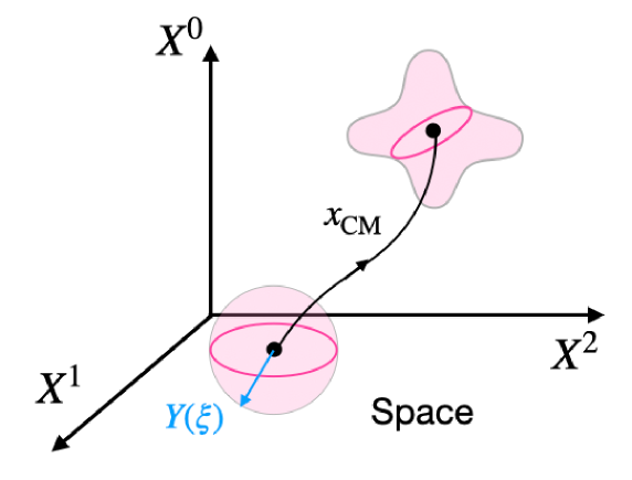
Figure 5: An illustration of the propagating $p$-brane in spacetime.

3.2 Born-Oppenheimer treatment

In general, the motion of $p$-brane is a complex mixture of the center-of-mass and relative motions as illustrated in Fig. 5. This situation reminds us molecular dynamics consisting of atomic nuclei and electrons. In particular, when we closely look at the equations (93)-(96), one can recognize that one of the complexities of the brane motion originates in the existence of $\mathrm{Vol}[C_{p}(t)]$ in each terms in the Lagrangian. In other words, the complexity seems to be significantly reduced when we separate the volume-dynamics from the others. Such a treatment resembles the Born-Oppenheimer approximation in molecule systems [34] and we consider a similar treatment in the $p$-brane dynamics below.

We neglect $\dot{\mathrm{Vol}}[C_{p}(t)]$ in Eq. (92) and the second term in Eq. (93), and represent a fixed $p$-brane volume as

$$\mathrm{Vol}[C_{p}]=V_{p}\quad\leftrightarrow\quad M_{p}[C_{p}]\coloneq T_{p}\mathrm{Vol}[C_{p}]=T_{p}V_{p}=M_{p}~,$$ (100)

where $M_{p}$ can be interpreted as the “mass” of $p$-brane. The validity of this Born-Oppenheimer treatment is discussed in the last part of this section. Within this approximation, one can see that the center-of-mass transition amplitude is decoupled from the relative motions in Eq. (98) and described by

$$\langle C_{p}|e^{-i(\hat{H}-i\varepsilon)A}|C_{p}^{{}^{\prime}}\rangle\bigg{|}_{\mathrm{CM}}=\int\frac{d^{D}k_{\mathrm{CM}}}{(2\pi)^{D}}e^{ik_{\mathrm{CM}}\cdot(x_{\mathrm{CM}}-x_{\mathrm{CM}}^{{}^{\prime}})-i\frac{AT_{p}^{2}}{2}\left(\frac{k_{\mathrm{CM}}^{2}}{M_{p}^{2}}-i\varepsilon\right)}~,$$ (101)

which coincides with the transition amplitude of relativistic particle with a proper time $AT_{p}/V_{p}$ and mass $M_{p}$.

As for the relative motions, we can at least find a self-consistent saddle-path in the following way. First, Eq. (96) can be deformed as

$$\int_{M_{p+1}}K_{p+1}=\frac{1}{(p+1)!}\int_{M_{p+1}}\bigg{[}d(K_{\mu_{1}\cdots\mu_{p+1}}(t,\xi)Y^{\mu_{1}})\wedge\cdots\wedge dY^{\mu_{p+1}}$$

$$\hskip 170.71652pt-(dK_{\mu_{1}\cdots\mu_{p+1}}(t,\xi))Y^{[\mu_{1}}dY^{\mu_{2}}\wedge\cdots\wedge dY^{\mu_{p+1}]}\bigg{]}$$

$$= \int_{C_{p}}K_{p}(A)-\int_{C_{p}^{{}^{\prime}}}K_{p}(0)-\frac{1}{(p+1)!}\int_{M_{p+1}}(dK_{\mu_{1}\cdots\mu_{p+1}}(t,\xi))Y^{[\mu_{1}}dY^{\mu_{2}}\wedge\cdots\wedge dY^{\mu_{p+1}]}$$ (102)

by the Stokes theorem. Then, if we neglect the $\{Y^{\mu}(t,\xi)\}$ dependence in Eq. (95) (i.e. $h(t,\xi)$), one can see that their dependence appears only in the last term in Eq. (102) in the exponent in the transition amplitude (98), leading to the following saddle-path condition

$$dK_{\mu_{1}\cdots\mu_{p+1}}(t,\xi)=0\quad\therefore K_{\mu_{1}\cdots\mu_{p+1}}(t,\xi)=k_{\mu_{1}\cdots\mu_{p+1}}=\text{constant}~,$$ (103)

as well as the center-of-mass momenta (97). By putting this into Eq. (95), one can check

$$K_{p}(t)^{2}=k\cdot k\coloneq\frac{1}{(p+1)!}k_{\mu_{1}\cdots\mu_{p+1}}k^{\mu_{1}\cdots\mu_{p+1}}~,$$ (104)

which is indeed independent of $\{Y^{\mu}(\xi)\}$. Thus, Eq. (103) can be regarded as one of the saddle-paths of the relative motions, although the existence of other saddle-paths cannot be ruled out.

Now the transition amplitude (98) in the Born-Oppenheimer and saddle-path approximations can be written as

$$\langle C_{p}|e^{-i\hat{H}A}|C_{p}^{{}^{\prime}}\rangle|_{\mathrm{BO}}$$

$$\approx \int\frac{d^{D}k_{\mathrm{CM}}}{(2\pi)^{D}}\int\frac{d^{D^{\prime}}k}{(2\pi)^{D^{\prime}}}\exp\left(ik_{\mathrm{CM}}\cdot(x_{\mathrm{CM}}-x_{\mathrm{CM}}^{{}^{\prime}})+ik\cdot(\sigma[C_{p}]-\sigma[C_{p}^{{}^{\prime}}])-i\frac{AT_{p}^{2}}{2}\left(\frac{k_{\mathrm{CM}}^{2}}{M_{p}^{2}}+\frac{k\cdot k}{T_{p}^{2}}+1-i\varepsilon\right)\right),$$ (105)

where $D^{\prime}={}_{D}C_{p+1}$ and

$$k\cdot\sigma[C_{p}]\coloneq\frac{1}{(p+1)!}k_{\mu_{1}\cdots\mu_{p+1}}\sigma^{\mu_{1}\cdots\mu_{p+1}}[C_{p}]~.$$ (106)

Compared to the transition amplitude of relativistic particle (101), Eq. (105) describes the propagation of the area elements $\sigma^{\mu_{1}\cdots\mu_{p+1}}[C_{p}]$ of $p$-brane as well. Note that the result (105) does not have any dependences on bulk quantities (fluctuations) in the present approximations.

Although a true propagator of $p$-brane would be more complicated than Eq. (105), it tells us how the motion of $p$-brane with a fixed-volume can vary according to the change of $T_{p}$ and $V_{p}$. For example, when

$$T_{p}\rightarrow\infty\quad\text{with}\quad M_{p}~=~\text{fixed}\quad(\text{Point-particle limit})~,$$ (107)

Eq. (105) becomes

$$\langle C_{p}|e^{-i\hat{H}A}|C_{p}^{{}^{\prime}}\rangle|_{\mathrm{BO}}\approx \delta^{(D^{\prime})}(\sigma[C_{p}]-\sigma[C_{p}^{{}^{\prime}}])\int\frac{d^{D}k_{\mathrm{CM}}}{(2\pi)^{D}}e^{ik_{\mathrm{CM}}\cdot(x_{\mathrm{CM}}-x_{\mathrm{CM}}^{{}^{\prime}})-i\frac{AT_{p}^{2}}{2}\left(\frac{k_{\mathrm{CM}}^{2}}{M_{p}^{2}}+1-i\varepsilon\right)},$$ (108)

which represents the propagation of relativistic particle. On the other hand, for

$$V_{p}\rightarrow\infty\quad\text{with}\quad T_{p}~=~\text{fixed}\quad(\text{Large-brane limit})~,$$ (109)

Eq. (105) becomes

$$\langle C_{p}|e^{-i\hat{H}A}|C_{p}^{{}^{\prime}}\rangle|_{\mathrm{BO}}\approx \delta^{(D)}(x_{\mathrm{CM}}-x_{\mathrm{CM}}^{{}^{\prime}})\int\frac{d^{D^{\prime}}k}{(2\pi)^{D^{\prime}}}e^{ik\cdot(\sigma[C_{p}]-\sigma[C_{p}^{{}^{\prime}}])-i\frac{A}{2}\left(k\cdot k+T_{p}^{2}-i\varepsilon\right)}~,$$ (110)

which describes the propagation of the shape-deformations of $p$-brane without changing the center-of-mass position. We should note that similar transition amplitude and propagator were derived in Refs. [37, 31, 32, 33] based on the first-quantized Polyakov action of $p$-brane in the mini-superspace and quenched approximations. In the present framework, such approximations correspond to the Born-Oppenheimer and saddle-path approximations.

Finally, let us discuss the conditions under which the Born-Oppenheimer approximation would be valid. Equation (105) leads to the following effective action for $\mathrm{Vol}[C_{p}(t)]$:

$$S_{\mathrm{eff}}=\int_{0}^{A}dt\left[k_{\mathrm{Vol}}(t)\dot{\mathrm{Vol}}[C_{p}(t)]-\frac{1}{2}\left(\frac{k^{2}}{M_{p}(t)^{2}}+D[C_{p}(t)]k_{\mathrm{Vol}}(t)^{2}\right)\right]~,\quad M_{p}(t)=T_{p}\mathrm{Vol}[C_{p}(t)]~.$$ (111)

One can see that the center-of-mass kinetic energy $k^{2}/M_{p}(t)^{2}$ plays a role of a potential for the volume dynamics. In order to compare several time-scales, let us use the dimensionless unit such that every quantities is normalized by an appropriate power of the $p$-brane tension $T_{p}$. Then, a typical (dimensionless) time-scale of the volume-dynamics $\tau_{\mathrm{Vol}}$ at a volume point $\mathrm{Vol}[C_{p}]=V_{p}$ can be roughly estimated as

$$\tau_{\mathrm{Vol}}\sim T_{p}\left(\bigg{|}D[V_{p}]\frac{(k^{2}/M_{p}^{2})^{\prime\prime}}{k^{2}/M_{p}^{2}}\bigg{|}\right)^{-\frac{1}{2}}\sim T_{p}\sqrt{\frac{V_{p}^{2}}{D[V_{p}]}}\sim T_{p}V_{p}^{\frac{p+1}{p}}~,$$ (112)

where ^′ denotes the derivative with respect to $V_{p}$. Here, we have used a naive dimensional analysis $D[V_{p}]\sim V_{p}^{-2/p}$ as it depends only on the volume-form of $C_{p}$. (See the definition (94).) On the other hand, the typical diffusion time-scales of the center-of-mass and area-elements can be read from Eq. (105) as

$$\tau_{\mathrm{CM}}\sim\tau_{\mathrm{AE}}\sim AT_{p}^{2}~,$$ (113)

which implies that the volume-dynamics is negligible as long as

$$s\coloneq\frac{AT_{p}}{V_{p}}\ll L_{p}\coloneq V_{p}^{\frac{1}{p}}~,$$ (114)

where $s$ can be interpreted as the proper-time and $L_{p}$ corresponds to the typical size of $p$-brane. Namely, the Born-Oppenheimer approximation seems to be invalid after the proper-time becomes comparable to the size of $p$-brane itself. In this sense, the point-particle limit (107) appears to be always invalid, wheres the large-brane limit (109) remains meaningful. A more dedicated study is necessary to understand the propagation of $p$-brane beyond the Born-Oppenheimer approximation.

3.3 Hausdorff dimension

Hausdorff dimension is a measure of fractal dimension of general objects [38]. In the case of closed $p$-brane, it can be generally defined based on the random-surface picture as follows. In a discretized Euclidean space such as a cubic lattice with a lattice size $a$, let us consider a random motion of $p$-brane such that one random step is described by adding a $p$-plaquette to a given $p$-brane as illustrated by the orange block in Fig. 2. After $A$ steps, we end up with another $p$-brane $C_{p}$ starting from an initial $p$-brane $C_{p}^{{}^{\prime}}$. Then, we count the number of triangulations constructed by $A$ $p$-plaquettes with an initial $p$-brane $C_{p}^{{}^{\prime}}$ and final $p$-brane $C_{p}$ as

$$n_{\chi}(C_{p},C_{p}^{{}^{\prime}};A)~,$$ (115)

where $\chi$ represents a topology of the random surfaces. Then, the total number of $A$-step triangulations starting from an initial $p$-brane $C_{p}^{{}^{\prime}}$ is given by

$$N_{\chi}(C_{p}^{{}^{\prime}};A)\coloneq\sum_{C_{p}}n_{\chi}(C_{p},C_{p}^{{}^{\prime}};A)~,$$ (116)

where the summation is taken over all $p$-branes in Euclidean spacetime. This allows us to define the probability distribution of finding a $p$-brane $C_{p}$ starting from an initial $p$-brane $C_{p}^{{}^{\prime}}$ as

$$P_{\chi}(C_{p},C_{p}^{{}^{\prime}};A)\coloneq\frac{n_{\chi}(C_{p},C_{p}^{{}^{\prime}};A)}{N_{\chi}(C_{p}^{{}^{\prime}};A)}~,$$ (117)

by which we can define the mean-square size of random surfaces as

$$\langle X^{2}\rangle_{A}\coloneq\sum_{C_{p}}P_{\chi}(C_{p},0;A)\left(x_{\mathrm{CM}}^{\mu}x_{\mathrm{CM}\mu}+(\sigma[C_{p}]\cdot\sigma[C_{p}])^{\frac{1}{p+1}}\right)~,$$ (119)

where we have taken the vanishing limit of the initial $p$-brane for simplicity. When this mean-square size behaves as

$$\langle X^{2}\rangle_{A}\sim A^{\frac{2}{D_{\mathrm{H}}}}\quad\leftrightarrow\quad A\sim\left(\sqrt{\langle X^{2}\rangle_{A}}\right)^{D_{\mathrm{H}}}$$ (120)

in the large $A$ limit, $D_{\mathrm{H}}$ represents the effective dimension of random surfaces, i.e. the Hausdorff dimension. Thus, we can in principle calculate $D_{\mathrm{H}}$ once a theory/model of random surfaces is given.

In the present brane-field theory, the Euclidean transition amplitude can be identified with the provability distribution as

$$P_{\chi}(C_{p},C_{p}^{{}^{\prime}};A)=\langle C_{p}|e^{-\hat{H}A}|C_{p}^{{}^{\prime}}\rangle~,$$ (121)

and the result (105) in the Born-Oppenheimer approximation leads

$$\langle X^{2}\rangle_{A}\propto\begin{cases}A&\text{(Point-particle limit)}\\ A^{\frac{1}{p+1}}&\text{(Large-brane limit)}\end{cases}$$ (122)

Then, from the definition of the Hausdorff dimension (120), we obtain

$$D_{\mathrm{H}}\approx\begin{dcases}2&(\text{Point-particle limit})\\ 2(p+1)&(\text{Large-brane limit})\end{dcases}$$ (123)

in the Born-Oppenheimer approximation. In particular, the Hausdorff dimension of random $1$-brane is $D_{\mathrm{H}}|_{p=1}=4$, as conjectured by Parisi in Ref. [42].

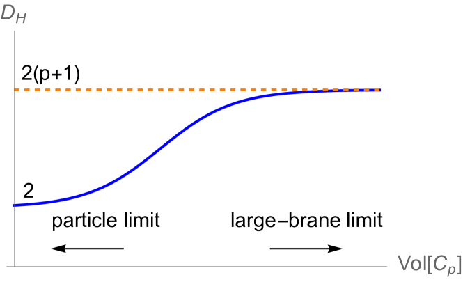
Figure 6: The Hausdorff dimension of $p$-brane as a function of its volume within the Born-Oppenheimer approximation.

Although it is not easy to examine the intermediate volume region analytically, we expect that $D_{\mathrm{H}}$ is smoothly connected between $2$ and $2(p+1)$ as illustrated in Fig. 6. Note that these results are valid only in the present brane-field model (26) and within the Born-Oppenheimer approximation. In fact, the Hausdorff dimension of non-critical closed string has been calculated in many literatures [39, 43, 44, 40, 41], yielding various predictions due to different definitions of the effective size. For example, in Ref. [39], the Hausdorff dimension is found to be dependent on the spacetime dimension (central charge) as $D_{\mathrm{H}}=-2/\gamma(D)$, where $\gamma(D)$ is the string susceptibility $\gamma(D)$.

4 Summary

We have studied phases and propagation of closed $p$-brane in the effective field theory with higher-form global symmetries. Compare to the previous studies [1, 2, 3, 19], we have included the kinetic term of the center-of-mass motion as well as the kinetic term constructed by the area derivatives, which then gives rise to a new dynamical scalar (NG) mode of the $0$-form global symmetry. Within the mean-field analysis, we have shown that the classical brane-field exhibits the area law in the unbroken phases in the large-brane limit and that the effective theory is described by the simple Maxwell theory (49) when the higher-form global symmetries are $\mathrm{U}(1)$. On the other hand, when these $\mathrm{U}(1)$ global symmetries are explicitly broken down to discrete ones, the effective theory in the broken phase is found to be a topological field theories such as Eq. (52) and (65) with multiple (emergent) higher-form discrete symmetries, resulting in topological order in general.

In addition to the mean-field analysis, we have investigated the propagation of $p$-brane in the present framework. Compared to the naive kinetic term employing the conventional functional derivatives, our brane-field model can be more intuitively analyzed due to (i) the separation of kinetic terms between the center-of-mass and relative motions and (ii) nice geometrical properties of the area derivatives. We have found the plane-wave solutions of the kinetic terms and obtained the path-integral expression of the brane propagator in the Schwinger’s proper time formalism. However, due to the mixture of the center-of-mass and relative motions, it is still challenging to perform the path-integral exactly. As a first step toward understanding the propagation of $p$-brane, we have applied the Born-Oppenheimer approximation by treating the brane volume as constant and obtained the approximate analytic expressions of the propagator: In the point-particle limit, the propagator reduces to the ordinary propagator of relativistic particle with the mass $M_{p}=T_{p}V_{p}$, while it describes the propagation of the area elements in the large-brane limit. Moreover, we have examined the Hausdorff dimension of $p$-brane and found that it varies from $2$ to $2(p+1)$ as the $p$-brane volume increases. While these results are intriguing, the Born-Oppenheimer approximation seems to be invalid for the point-particle limit, suggesting that the quantum nature of $p$-brane is essentially different from relativistic particle for any parameter values. A more dedicated analysis is left for future investigations.

Appendix A Functional Derivative

In this Appendix, we summarize the basics of ordinary functional derivatives. Let us consider a functional $F[\phi]$ of a scalar field $\phi(X)$. A naive functional derivative at a point $X$ can be defined by

$$\frac{\delta F[\phi]}{\delta\phi(X)}=\lim_{\varepsilon\rightarrow 0}\frac{F[\phi(Y)+\varepsilon\delta^{(d)}(Y-X)]-F[\phi]}{\varepsilon}~,$$ (124)

which is not manifestly covariant because the delta function is not. Instead, we can define a manifestly covariant functional derivative by

$$\frac{\delta_{c}F[\phi]}{\delta\phi(X)}=\lim_{\varepsilon\rightarrow 0}\frac{F[\phi(Y)+\varepsilon\delta_{c}^{(d)}(Y-X)]-F[\phi]}{\varepsilon}~,$$ (125)

where

$$\delta_{c}^{(d)}(Y-X)\coloneqq\frac{1}{\sqrt{-g(X)}}\delta^{(d)}(Y-X)$$ (126)

is the covariant delta function. In particular, when $F[\phi]=\phi(X)$, we have

$$\frac{\delta_{c}\phi(X)}{\delta\phi(Y)}=\delta^{(d)}_{c}(X-Y)~,$$ (127)

and one can check that Eqs. (124)(125) are related each other as

$$\frac{\delta_{c}F[\phi]}{\delta\phi(X)}=\int d^{d}Y\frac{\delta_{c}\phi(Y)}{\delta\phi(X)}\frac{\delta_{c}F[\phi]}{\delta_{c}\phi(Y)}=\frac{1}{\sqrt{-g(X)}}\frac{\delta F[\phi]}{\delta\phi(X)}~.$$ (128)

Then, a general functional expansion is

$$F[\phi+\delta\phi] =\sum_{n=0}^{\infty}\frac{1}{n!}\left(\prod_{i=1}^{n}\int d^{d}X_{i}\sqrt{-g(X)}\delta\phi(X_{i})\right)\frac{\delta^{n}_{c}F[\phi]}{\delta\phi(X_{1})\cdots\delta\phi(X_{n})}$$ (129)

$$=\sum_{n=0}^{\infty}\frac{1}{n!}\left(\prod_{i=1}^{n}\int d^{d}X_{i}\delta\phi(X_{i})\right)\frac{\delta^{n}F[\phi]}{\delta\phi(X_{1})\cdots\delta\phi(X_{n})}~.$$ (130)

References

- [1] Y. Hidaka and K. Kawana, Effective brane field theory with higher-form symmetry, JHEP 01 (2024), 016, 2310.07993.
- [2] K. Kawana, Field theory for superconducting branes and generalized particle-vortex duality, JHEP 11 (2024), 066, 2406.03670.
- [3] K. Kawana, Classical continuum limit of the string field theory dual to lattice gauge theory, Progress of Theoretical and Experimental Physics (2025), ptaf023, https://academic.oup.com/ptep/advance-article-pdf/doi/10.1093/ptep/ptaf023/61779122/ptaf023.pdf.
- [4] D. Gaiotto, A. Kapustin, N. Seiberg, and B. Willett, Generalized Global Symmetries, JHEP 02 (2015), 172, 1412.5148.
- [5] A. Kapustin, Wilson-’t Hooft operators in four-dimensional gauge theories and S-duality, Phys. Rev. D 74 (2006), 025005, hep-th/0501015.
- [6] T. Pantev and E. Sharpe, GLSM’s for Gerbes (and other toric stacks), Adv. Theor. Math. Phys. 10 (2006), no. 1, 77–121, hep-th/0502053.
- [7] Z. Nussinov and G. Ortiz, A symmetry principle for topological quantum order, Annals Phys. 324 (2009), 977–1057, cond-mat/0702377.
- [8] T. Banks and N. Seiberg, Symmetries and Strings in Field Theory and Gravity, Phys. Rev. D 83 (2011), 084019, 1011.5120.
- [9] A. Kapustin and R. Thorngren, Higher symmetry and gapped phases of gauge theories, (2013), 1309.4721.
- [10] O. Aharony, N. Seiberg, and Y. Tachikawa, Reading between the lines of four-dimensional gauge theories, JHEP 08 (2013), 115, 1305.0318.
- [11] A. Kapustin and N. Seiberg, Coupling a QFT to a TQFT and Duality, JHEP 04 (2014), 001, 1401.0740.
- [12] D. Gaiotto, A. Kapustin, Z. Komargodski, and N. Seiberg, Theta, Time Reversal, and Temperature, JHEP 05 (2017), 091, 1703.00501.
- [13] J. McGreevy, Generalized Symmetries in Condensed Matter, (2022), 2204.03045.
- [14] T. D. Brennan and S. Hong, Introduction to Generalized Global Symmetries in QFT and Particle Physics, (2023), 2306.00912.
- [15] L. Bhardwaj, L. E. Bottini, L. Fraser-Taliente, L. Gladden, D. S. W. Gould, A. Platschorre, and H. Tillim, Lectures on Generalized Symmetries, (2023), 2307.07547.
- [16] R. Luo, Q.-R. Wang, and Y.-N. Wang, Lecture Notes on Generalized Symmetries and Applications, (2023), 2307.09215.
- [17] P. R. S. Gomes, An introduction to higher-form symmetries, SciPost Phys. Lect. Notes 74 (2023), 1, 2303.01817.
- [18] S.-H. Shao, What’s Done Cannot Be Undone: TASI Lectures on Non-Invertible Symmetry, (2023), 2308.00747.
- [19] N. Iqbal and J. McGreevy, Mean string field theory: Landau-Ginzburg theory for 1-form symmetries, SciPost Phys. 13 (2022), 114, 2106.12610.
- [20] T. Eguchi, New Approach to the Quantized String Theory, Phys. Rev. Lett. 44 (1980), 126.
- [21] A. T. Ogielski, Comments on the ’Planar Time’ Dynamics of Strings, Phys. Rev. D 22 (1980), 2407.
- [22] T. Yoneya, A Path Functional Field Theory of Lattice Gauge Models and the Large Limit, Nucl. Phys. B 183 (1981), 471–496.
- [23] T. Banks, THE GAUSSIAN TRANSFORMATION CONVERTS LATTICE GAUGE THEORY INTO A FIELD THEORY OF STRINGS, Phys. Lett. B 89 (1980), 369–372.
- [24] A. A. Migdal, Loop Equations and 1/N Expansion, Phys. Rept. 102 (1983), 199–290.
- [25] Y. Makeenko and A. A. Migdal, Quantum Chromodynamics as Dynamics of Loops, Sov. J. Nucl. Phys. 32 (1980), 431.
- [26] A. M. Polyakov, Gauge Fields as Rings of Glue, Nucl. Phys. B 164 (1980), 171–188.
- [27] H. Kawai, A Dual Transformation of the Nielsen-olesen Model, Prog. Theor. Phys. 65 (1981), 351.
- [28] S.-J. Rey, Higgs mechanism for kalb-ramond gauge field, Phys. Rev. D 40 (1989), 3396–3401.
- [29] Y. Hidaka, M. Nitta, and R. Yokokura, Topological axion electrodynamics and 4-group symmetry, Phys. Lett. B 823 (2021), 136762, 2107.08753.
- [30] Y. Hidaka, M. Nitta, and R. Yokokura, Selection rules of topological solitons from non-invertible symmetries in axion electrodynamics, (2024), 2411.05434.
- [31] S. Ansoldi, A. Aurilia, and E. Spallucci, Hausdorff dimension of a quantum string, Phys. Rev. D 56 (1997), 2352–2361, hep-th/9705010.
- [32] S. Ansoldi, A. Aurilia, C. Castro, and E. Spallucci, Quenched, minisuperspace, bosonic p-brane propagator, Phys. Rev. D 64 (2001), 026003, hep-th/0105027.
- [33] A. Aurilia, S. Ansoldi, and E. Spallucci, Fuzzy dimensions and Planck’s uncertainty principle for p branes, Class. Quant. Grav. 19 (2002), 3207–3216, hep-th/0205028.
- [34] M. BORN and R. OPPENHEIMER, ON THE QUANTUM THEORY OF MOLECULES, 1–24, pp. 1–24.
- [35] Y. Nambu, Generalized hamiltonian dynamics, Phys. Rev. D 7 (1973), 2405–2412.
- [36] K. Kawana, Classical Continuum Limit of the String Field Theory Dual to Lattice Gauge Theory, (2024), 2410.08552.
- [37] S. Ansoldi, A. Aurilia, and E. Spallucci, String propagator: A Loop space representation, Phys. Rev. D 53 (1996), 870–878, hep-th/9510133.
- [38] T. Gneiting, H. Ševčíková, and D. B. Percival, Estimators of fractal dimension: Assessing the roughness of time series and spatial data, Statistical Science 27 (2012), no. 2.
- [39] J. Distler, Z. Hlousek, and H. Kawai, Hausdorff Dimension of Continuous Polyakov’s Random Surfaces or Who’ Afraid of Joseph Liouville? Part 2, Int. J. Mod. Phys. A 5 (1990), 1093.
- [40] J. Ambjorn, D. Boulatov, J. L. Nielsen, J. Rolf, and Y. Watabiki, The Spectral dimension of 2-D quantum gravity, JHEP 02 (1998), 010, hep-th/9801099.
- [41] J. Ambjørn and T. Budd, The toroidal Hausdorff dimension of 2d Euclidean quantum gravity, Phys. Lett. B 724 (2013), 328–332, 1305.3674.
- [42] G. Parisi, Hausdorff Dimensions and Gauge Theories, Phys. Lett. B 81 (1979), 357–360.
- [43] H. Kawai, Quantum gravity and random surfaces, Nucl. Phys. B Proc. Suppl. 26 (1992), 93–110.
- [44] H. Kawai, N. Kawamoto, T. Mogami, and Y. Watabiki, Transfer matrix formalism for two-dimensional quantum gravity and fractal structures of space-time, Phys. Lett. B 306 (1993), 19–26, hep-th/9302133.