Online Optimization with Unknown Time-varying Parameters

Abstract

In this paper, we study optimization problems where the cost function contains time-varying parameters that are unmeasurable and evolve according to linear, yet unknown, dynamics. We propose a solution that leverages control theoretic tools to identify the dynamics of the parameters, predict their evolution, and ultimately compute a solution to the optimization problem. The identification of the dynamics of the time-varying parameters is done online using measurements of the gradient of the cost function. This system identification problem is not standard, since the output matrix is known and the dynamics of the parameters must be estimated in the original coordinates without similarity transformations. Interestingly, our analysis shows that, under mild conditions that we characterize, the identification of the parameters dynamics and, consequently, the computation of a time-varying solution to the optimization problem, requires only a finite number of measurements of the gradient of the cost function. We illustrate the effectiveness of our algorithm on a series of numerical examples.

I Introduction

Mathematical optimization is a fundamental tool used across diverse applications, ranging from robotics [1], control [2], and machine learning [3]. It offers a structured framework for expressing objectives and defining constraints, enabling a systematic approach to finding the most favorable solutions in diverse contexts. Recently, there has been a significant interest in time-varying optimization problems due to their ability to capture the complexity of dynamic environments and changing optimization objectives. In such problems, the cost parameters vary with time, and optimization algorithms must adapt in real-time and incorporate new information to track the optimal time-varying solution [4, 5]. In this work, we consider the following optimization problem with time-varying parameters

$$\min_{x\in\mathbb{R}^{n}}~~f(x,z(t))=g(x)^{\mathsf{T}}z(t),\quad t\geq 0$$ (1)

where $f:\mathbb{R}^{n}\times\mathbb{R}^{p}\rightarrow\mathbb{R}$ is the cost function with time varying parameters $z(t)\in\mathbb{R}^{p}$, and $g:\mathbb{R}^{n}\rightarrow\mathbb{R}^{p}$ is a vector-valued function whose entries depend on $x$. The parameters $z(t)$ are not measurable and evolve with linear, yet unknown, dynamics. Our objective is to develop an online algorithm to compute and track the optimal solution of (1) using measurements of the gradient of the cost function. In particular, we propose a solution that leverages control theoretic tools to identify the exact dynamics of the parameters $z(t)$, predict their evolution, and ultimately compute the optimal solution. Interestingly, our analysis shows that the identification of the cost function and, consequently, the computation of the optimal time-varying solution to (1) requires only a finite number of measurements of the gradient of the cost function.

Related work. Several methods for solving time-varying optimization problems have been studied in the literature. These methods can be categorized into two classes, namely unstructured methods and structured methods. Unstructured methods are passive and do not leverage the dynamics of the optimization problem: each time-instance of the optimization problem is treated as a static problem and solved using static optimization algorithms (e.g., gradient descent) [6, 7, 8, 9]. Since these methods ignore the dynamic nature of the problem and make decisions only after observing a time instance of the cost, convergence to the optimal time-varying solution is never achieved and is only guaranteed to a neigberhood of the optimal solution [10, 5, 11, 12]. On the counter part, structured algorithms leverage the dynamics of the problem in order to achieve exact tracking of the time-varying optimal solution [5]. A particular class of algorithms that fall under structured methods is the prediction-correction algorithms. At each time-step, a prediction step is used to forecast how the optimal solution evolves with time, followed by a correction step to update the solution. The prediction-correction algorithm has been studied in the literature in continuous-time [13, 14, 15] and discrete-time [16, 17, 18]. In the recent work [19], the authors study quadratic optimization problems with time-varying linear term, where they leveraged control theoretic tools to develop a structured online algorithm that achieves zero-tracking error asymptotically. In [20], the authors extended the work of [19] by studying quadratic optimization problems with inequality constraints where the linear term in the cost and the inequality values are time-varying. In this work, we focus on optimization problems as in (1), where we propose a solution that leverages control theoretic tools to identify the exact dynamics of the coefficients, $z(t)$, predict their evolution, and ultimately compute the optimal solution. However, differently from [19, 20], we have all the cost parameters $z(t)$ in (1) varying with time as opposed to only varying the linear term. Recent works [21, 22] have explored time-varying cost functions where temporal variability arises from the time-varying parameters. These works consider a general cost function with unknown parameters that vary linearly, assuming either the parameters are known or the dynamics of these parameters are known, or both the parameters and their dynamics are known. In contrast, our work addresses a more general setting where neither the parameters nor their dynamics are known. However, we do restrict our analysis to cost functions expressed as (1).

Contributions. The main contributions of this paper are as follows. First, we design an algorithm to solve the time-varying optimization problem (1), which requires the identification of the dynamics of the parameters in the cost using measurements of the gradient of the cost function. This system identification problem is not standard, since the output matrix is known and the dynamics of the parameters must be estimated in the original coordinates without similarity transformations. Second, we provide a set of conditions on the parameters dynamics and gradient measurements that guarantee the solvability of the parameters identification problem using only a finite number of gradient measurements. Third and finally, we illustrate the effectiveness of our algorithm on a series of examples.

Notation. The $n\!\times\!n$ identity matrix is denoted by $I_{n}$. The Kronecker product is denoted by $\otimes$. The left (right) pseudo inverse of a tall (fat) matrix $A$ is denoted by $A^{\dagger}$. The column-space of a matrix $A$ is denoted by $\operatorname{Col}{\left(A\right)}$. The dimension of a subspace $\mathcal{V}$ is denoted by $\dim{\left(\mathcal{V}\right)}$. The range-space and the null-space of a matrix $A$ are denoted by $\text{Im}\left(A\right)$ and $\text{Ker}\left(A\right)$, respectively. For a matrix $A\!\in\!\mathbb{R}^{n\times m}$, let $\text{vec}\!\left(A\right)\!\in\!\mathbb{R}^{nm}$ denotes the vectorization of $A$, which is obtained by stacking the columns of $A$ on top of one another, and $\text{vec}^{-1}\!\left(\cdot\right)$ denotes the inverse vectorization operator, i.e., $\text{vec}^{-1}\!\left(\text{vec}\!\left(A\right)\right)=A$. The complement set and the cardinality of a set $\mathcal{S}$ are denoted by $\mathcal{S}^{\text{c}}$ and $|\mathcal{S}|$, respectively.

II Problem formulation

Consider the time-varying optimization problem (1). Let the parameters $z(t)$ evolve according to the following discrete-time, linear, time-invariant dynamics:

$$z(t+1)=Az(t),$$ (2)

where $A\in\mathbb{R}^{p\times p}$. We assume that the matrix $A$ is unknown, and that the parameters $z$ are not measurable. However, we assume that, at each time, an Oracle can provide the value of the gradient of the cost function $f$ in (1) with respect to $x$ evaluated at a desired point $x\in\mathbb{R}^{n}$. Notice that

$$\underbrace{\frac{\partial f}{\partial x}\bigg{|}_{x}}_{y(x,t)}=\underbrace{\frac{\partial g^{\mathsf{T}}}{\partial x}\bigg{|}_{x}}_{C(x)}z(t).$$ (3)

In other words, the gradient of the cost function evaluated at a desired point $x$ is a linear function of the parameters $z$, which can be used as a linear output to simultaneously identify the parameters dynamics, predict their trajectory, and ultimately solve the time-varying optimization problem (1). It should be noticed that the identification of the parameters dynamics is a nonstandard system identification problem, because the output matrix $C(x)$ is known yet dependent on the optimization variable $x$, and because the parameters dynamics (2) need to be identified in their original coordinates rather than up to an arbitrary similarity transformation. In fact, a similarity transformation of (2) would yield an incorrect set of parameters and ultimately an incorrect solution to (1). We make the following assumptions on the parameter dynamics (2) and their initial state $z(0)$ that hold throughout the letter:

• The matrix $A$ in (2) has distinct and non-zero eigenvalues.

• The pair $(A,z(0))$ is controllable.

While Assumption (A1) is a technical condition that simplifies the notation and analysis, Assumption (A2) is generically satisfied and necessary for the solvability of the identification and estimation problems. Also, Assumption (A2) ensures that the initial condition $z(0)$ excites all the modes of the system (2).

Example 1.

Consider the time-varying optimization problem,

$$\min_{x\in\mathbb{R}^{2}}~f(x,z(t))= z_{1}(t)x_{1}+z_{2}(t)x_{1}x_{2}+z_{3}(t)x_{1}^{2}+z_{4}(t)x_{2}^{2}$$

$$+z_{5}(t)\cos(x_{1})+z_{6}(t)\sin(x_{2}),\quad t\geq 0,$$

where $f:\mathbb{R}^{2}\times\mathbb{R}^{6}\rightarrow\mathbb{R}$ is the cost function, $x=[x_{1},x_{2}]^{\mathsf{T}}$ is the optimization variable, and $z(t)=[z_{1}(t),z_{2}(t),z_{3}(t),z_{4}(t),z_{5}(t),z_{6}(t)]^{\mathsf{T}}$ are the time-varying parameters of the cost. We can write $f(x,z(t))=g(x)^{\mathsf{T}}z(t)$ with $g(x)^{\mathsf{T}}=\begin{bmatrix}x_{1}&x_{1}x_{2}&x_{1}^{2}&x_{2}^{2}&\cos(x_{1})&\sin(x_{2})\end{bmatrix}$. Let $z(t)$ evolve with time according to the linear dynamics in (2), then, we can write the gradient measurement evaluated at $x$ as

$$\underbrace{\frac{\partial f}{\partial x}\bigg{|}_{x}}_{y(x,t)}=\underbrace{\begin{bmatrix}1&x_{2}&2x_{1}&0&-\sin(x_{1})&0\\ 0&x_{1}&0&2x_{2}&0&\cos(x_{2})\end{bmatrix}}_{C(x)}z(t).$$

$\square$

III Estimating the parameters and their dynamics

In this section we detail our method to identify the unknown parameters and their dynamics (2) to solve the time-varying optimization problem (1). Our approach consists of three mains steps, namely, (i) the identification of the parameter dynamics up to a similarity transformation using subspace identification techniques, (ii) the identification of the similarity transformation to recover the exact parameters dynamics using the knowledge of the output matrix $C(x)$, and (iii) the prediction of the parameters trajectory and the computation of a time-varying minimizer of (1). For notational convenience, let $y(t)=y(x(t),t)$, where $x(t)$ is the value at time $t$ at which the gradient $y(x,t)$ is evaluated. Let $X$ and $Y$ be the data collected from the Oracle over time, where $N\in\mathbb{N}$ and

$$X=\begin{bmatrix}x(0)&\cdots&x(N)\end{bmatrix},\quad Y=\begin{bmatrix}y(0)&\cdots&y(N)\end{bmatrix}.$$ (4)

Further, let the data matrices $X$ and $Y$ be partitioned as

$$X=\begin{bmatrix}X_{0}&X_{1}\end{bmatrix},\quad Y=\begin{bmatrix}Y_{0}&Y_{1}\end{bmatrix},$$ (5)

where $X_{0}$ and $Y_{0}$ contain the first $N_{0}=2p-2$ samples of $X$ and $Y$, respectively, and $X_{1}$ and $Y_{1}$ the remaining samples. We make the following assumptions:

• The pair $(A,C(x_{0}))$ is observable, where $x_{0}$ is the point at which the gradient $y(x,t)$ is evaluated at time $t=0$.

• The values $x(t)$ remain constant up to time $N_{0}$, that is, for $0\leq t\leq N_{0}$ and some vector $x_{0}\in\real^{n}$, $x(t)=x_{0}$.

Assumption (A3) is generically satisfied and necessary for the solvability of the identification and estimation problems. Assumption (A4) implies that the output matrix $C(x)$ and the data matrix $X_{0}$ are constant. This allows for the use of standard subspace identification techniques and simplifies the derivations, and it is compatible with settings where the Oracle can arbitrarily select the gradient evaluation points. Additionally, since $x(t)$ remains constant only for a finite time interval, this assumption induces only a finite delay in the computation of the solution to the optimization problem. Note that the time $N_{0}$ depends linearly on the system dimension $p$. That is, more complex cost functions (i.e., more parameters) induce a larger delay. The use of a non-constant matrix $C(x)$ and data matrix $X$ remains the topic of current investigations. We rewrite $Y_{0}$ in (5) in the following Hankel matrix form:

$$Y_{\text{h}}=\begin{bmatrix}y(0)&\cdots&y(p-1)\\ \vdots&\ddots&\vdots\\ y(p-1)&\cdots&y(2p-2)\end{bmatrix}.$$ (6)

The above Hankel matrix satisfies the following relation:

$$Y_{\text{h}}=\underbrace{\begin{bmatrix}C(x_{0})\\ C(x_{0})A\\ \vdots\\ C(x_{0})A^{p-1}\end{bmatrix}}_{O(x_{0})}\underbrace{\begin{bmatrix}z(0)&Az(0)&\cdots&A^{p-1}z(0)\end{bmatrix}}_{Z(0)}.$$ (7)

Since $C(x_{0})$ and $z(0)$ satisfy Assumptions (A2) and (A3), we have $\operatorname{Rank}{\left(Y_{\text{h}}\right)}=p$. To estimate $A$, we make use of the shift structure of the observability matrix $O(x_{0})$ as in [23], i.e.,

$$A=O_{1}^{\dagger}O_{2},$$ (8)

where $O_{1}$ and $O_{2}$ are matrices containing the first $n(p-1)$ rows of $O(x_{0})$ and the last $n(p-1)$ rows of $O(x_{0})$, respectively. We now factor $Y_{\text{h}}$ in (6) using the singular value decomposition, $Y_{\text{h}}=U\Sigma V^{\mathsf{T}}$, and construct the observability matrix from the left singular vectors, $U$, corresponding to the non-zero singular values. Notice that, because of Assumptions (A2) and (A3), we have $\operatorname{Col}{\left(Y_{\text{h}}\right)}=\operatorname{Col}{\left(O(x_{0})\right)}$. Hence, we have $\overline{O}(x_{0})\!=\!O(x_{0})T^{-1}\!=\!\overline{U}$, where $T\!\in\!\mathbb{R}^{p\times p}$ is a transformation matrix and $\overline{U}$ contains the left singular vectors of $Y_{\text{h}}$ corresponding to the non-zero singular values. Then,

$$\overline{A}=(\overline{O}_{1})^{\dagger}\overline{O}_{2},$$ (9)

where the matrices $\overline{O}_{1}$ and $\overline{O}_{2}$ contain the first $n(p-1)$ rows of $\overline{O}(x_{0})$ and the last $\left.n(p-1)\right.$ rows of $\overline{O}(x_{0})$, respectively. By construction, $\overline{A}$ is similar to $A$ in the parameters dynamics, that is, $A=T^{-1}\overline{A}T$, for some invertible matrix $T$. Next, we estimate the matrix $T$.

Using the notation in (7), let

$$\overline{Z}(0)=TZ(0)=\begin{bmatrix}\overline{z}(0)&\cdots&\overline{z}(p-1)\end{bmatrix}={\overline{O}(x_{0})}^{\dagger}Y_{\text{h}},$$ (10)

and, to simplify the notation, let $C(t)=C(x(t))$. Using [25, Proposition 7.1.9] and letting $\overline{z}=Tz$, we have

$$y(t)=\overline{C}(t)\overline{z}(t) =C(t)T^{-1}\overline{z}(t)$$

$$=\left(\overline{z}(t)^{\mathsf{T}}\otimes C(t)\right)\text{vec}\!\left(T^{-1}\right).$$

Consequently, we can write $Y_{1}$ in (5) as

$$\underbrace{\begin{bmatrix}y(N_{0}+1)\\ \vdots\\ y(N)\end{bmatrix}}_{Y_{\text{v}}=\text{vec}\left(Y_{1}\right)}=\underbrace{\begin{bmatrix}{\overline{z}(N_{0}+1)}^{\mathsf{T}}\otimes C(N_{0}+1)\\ \vdots\\ {\overline{z}(N)}^{\mathsf{T}}\otimes C(N)\end{bmatrix}}_{M}\text{vec}\!\left(T^{-1}\right).$$ (11)

Note that the matrix $M$ in (11) is known since we can compute $\overline{z}(N_{0}+1),\cdots,\overline{z}(N)$ by propagating $\overline{z}(p-1)$ in (10) using the matrix $\overline{A}$ in (9), and $C(N_{0}+1),\cdots,C(N)$ are computed using $X_{1}$ in (5). Then, using (11), we can compute $T$ as

$$T=\left(\text{vec}^{-1}\!\left(M^{\dagger}Y_{\text{v}}\right)\right)^{-1}.$$ (12)

and, finally, the exact realization $A$ in (2) as

$$A=T^{-1}\overline{A}T.$$

This procedure relies on the matrix $M$ in (11) being full column rank, which we characterize in the next results.

Theorem III.1.

(Necessary condition for the rank of $M$ in (11)) The matrix $M$ in (11) is full column-rank only if the matrix ${[C{(N_{0}+1)}^{\mathsf{T}}\cdots{C(N)}^{\mathsf{T}}]}^{\mathsf{T}}$ is full rank.

Proof:

Suppose $M$ in (11) is full column-rank. Then,

$$\bigcap_{i=N_{0}+1}^{N}\text{Ker}\left(\overline{z}(i)^{\mathsf{T}}\otimes C(i)\right)=0.$$ (13)

Using Lemma E-A.1, we re-write (13) as

$$\bigcap_{i=N_{0}+1}^{N}\!\text{Ker}\left(\overline{z}(i)^{\mathsf{T}}\!\otimes\!I_{p}\right)\cup\text{Ker}\left(I_{p}\!\otimes\!C(i)\right)\!=\!0.$$ (14)

For notational convenience, we use $\mathcal{A}(i)$ and $\mathcal{B}(i)$ to denote $\text{Ker}\left(\overline{z}(i)^{\mathsf{T}}\!\otimes\!I_{p}\right)$ and $\text{Ker}\left(I_{p}\!\otimes\!C(i)\right)$ for $i\!\in\!\{N_{0}\!+\!1,\!\cdots\!,N\}$, respectively. Expanding the terms in (14), we can write

$$\begin{split}\bigcup_{\mathcal{S}\subseteq\{N_{0}+1,\cdots,N\}}\left(\bigcap_{i\in\mathcal{S}}\mathcal{A}(i)\cap\bigcap_{j\in\mathcal{S}^{\text{c}}}\mathcal{B}(j)\right)=0.\end{split}$$ (15)

Since the union of all the terms in (15) is zero, then, each term of the union in (15) is zero. Hence, we have

$$\bigcap_{i=N_{0}+1}^{N}\mathcal{B}(i) =\bigcap_{i=N_{0}+1}^{N}\text{Ker}\left(I_{p}\otimes C(i)\right)=0.$$ (16)

Let $K_{i}$ be a matrix whose columns span $C(i)$. Then, using Lemma E-A.2, equation (16) can be equivalently written as

$$\bigcap_{i=N_{0}+1}^{N}\operatorname{Col}{\left(I_{p}\otimes K_{i}\right)} =0.$$ (17)

Equation (17) implies that

$$\begin{bmatrix}I_{p}\otimes C(N_{0}+1)\\ \vdots\\ I_{p}\otimes C(N)\end{bmatrix}(I_{p}\otimes K)=0\iff K=0.$$

Equivalently, we have

$$\begin{bmatrix}C(N_{0}+1)\\ \vdots\\ C(N)\end{bmatrix}K=0\iff K=0.$$

Which implies that ${[C{(N_{0}+1)}^{\mathsf{T}}\cdots{C(N)}^{\mathsf{T}}]}^{\mathsf{T}}$ is full rank. ∎

Theorem III.2.

(Necessary and sufficient condition for the rank of $M$ in (11)) Let $\overline{A}$ in (9) be diagonalizable and let $D$ be its diagonal form. Let $\left.\Lambda=D\otimes I_{p}\right.$ and $F(t)={\mathds{1}_{p}}^{\mathsf{T}}\otimes C(t)$, for $t\geq 0$. Then, the matrix $M$ in (11) is full column-rank if and only if the following matrix is full column-rank:

$$W=\begin{bmatrix}[c]F(N_{0}+1)\\ F(N_{0}+2)\Lambda\\ \vdots\\ F(N)\Lambda^{N-N_{0}-1}\end{bmatrix}.$$

$\square$

Proof:

From Assumption (A1), we have $A$ in (2) is diagonalizable. Hence, $\overline{A}$ in (9) is diagonalizable. Let $D$ be the diagonal form of $\overline{A}$, i.e., $D=U^{-1}\overline{A}U$, where $U$ is a matrix whose columns are the eigenvectors of $\overline{A}$. Let $\xi(t)=U^{-1}\overline{z}(t)$ for $t\geq 0$. Then, we can write $M$ in (11) as

$$\begin{split}M&=\begin{bmatrix}{\xi(N_{0}+1)}^{\mathsf{T}}U^{\mathsf{T}}\otimes C(N_{0}+1)\\ \vdots\\ {\xi(N)}^{\mathsf{T}}U^{\mathsf{T}}\otimes C(N)\end{bmatrix}\\ &=\underbrace{\begin{bmatrix}{\xi(N_{0}+1)}^{\mathsf{T}}\otimes C(N_{0}+1)\\ \vdots\\ {\xi(N)}^{\mathsf{T}}\otimes C(N)\end{bmatrix}}_{Q}(U^{\mathsf{T}}\otimes I_{p}).\end{split}$$ (18)

It follows from [25, Fact 7.4.24] that the matrix $U^{\mathsf{T}}\otimes I_{p}$ is full-rank. Then, $M$ in (11) is full-rank if and only if $Q$ in (18) is full-rank. Next, we provide necessary and sufficient condition such that $Q$ is full-rank. Each block row of $Q$ can be written as

$$\begin{split}\xi(t)^{\mathsf{T}}\otimes C(t)&\!=\!\begin{bmatrix}\xi_{1}(t)C(t)&\xi_{2}(t)C(t)&\cdots&\xi_{p}(t)C(t)\end{bmatrix}\\ &\!=\!\underbrace{\begin{bmatrix}C(t)&\cdots&C(t)\end{bmatrix}}_{F(t)}\!\!\underbrace{\begin{bmatrix}\xi_{1}(t)I_{p}&\cdots&0\\ 0&\cdots&0\\ \vdots&\ddots&\vdots\\ 0&\cdots&\xi_{p}(t)I_{p}\end{bmatrix}}_{\Xi(t)},\end{split}$$ (19)

where $\xi_{1},\cdots,\!\xi_{p}$ are the components of $\xi$ for $t\!\in\!\{N_{0}\!+\!1,\!\cdots,N\}$. Let $\Lambda=D\otimes I_{p}$. By noting that $\Xi(t+1)=\Lambda\Xi(t)$ and using the representation in (19), we can write $Q$ in (18) as

$$Q=\underbrace{\begin{bmatrix}F(N_{0}+1)\\ F(N_{0}+2)\Lambda\\ \vdots\\ F(N)\Lambda^{N-N_{0}-1}\end{bmatrix}}_{W}\Xi(N_{0}+1),$$ (20)

From Assumption (A2), $\Xi(N_{0}+1)$ is full-rank. Hence, $Q$ in (18) is full-rank if and only if the matrix $W$ in (20) is full-rank. Therefore, $M$ is full-rank if and only if $W$ is full-rank. ∎

IV Numerical examples and comparisons

We now present a series of numerical studies to validate the effectiveness of the proposed optimization algorithm.

IV-A Time-varying quadratic optimization

We consider a quadratic time-varying optimization problem as $f(x)=x^{\mathsf{T}}H(t)x+b(t)^{\mathsf{T}}x$, where $x\in\mathbb{R}^{2}$ and parameters $H(t)$ and $b(t)$ unknown. We assume that $H(t)\succ 0$ for all $t\geq 0$ is a symmetric matrix. We express this quadratic cost in the form (1) as

$$f(x,z(t))=\begin{bmatrix}x_{1}&x_{2}&x_{1}^{2}&2x_{1}x_{2}&x_{2}^{2}\end{bmatrix}z(t),$$ (21)

where $z(t)=[b_{1}(t),b_{2}(t),h_{11}(t),h_{12}(t),h_{22}(t)]^{\mathsf{T}}$. The unknown parameter $z(t)$ obeys the dynamics in (2) with $A=\mathrm{blkdiag}([E,F])$, $E\!=\!\begin{bmatrix}0&1\\ -1&0\end{bmatrix}$, and $F\!=\!\operatorname{diag}[0.98,0.95,0.981]$. We let $z(0)\!=\![-85.8,-77.9,1047,329,669]^{\mathsf{T}}$. The gradient of (21) is

$$y(x,t)=\begin{bmatrix}1&0&2x_{1}&2x_{2}&0\\ 0&1&0&2x_{1}&2x_{2}\end{bmatrix}z(t).$$ (22)

We use $N_{0}=8$ and $N=26$ for the data collection as in (4).

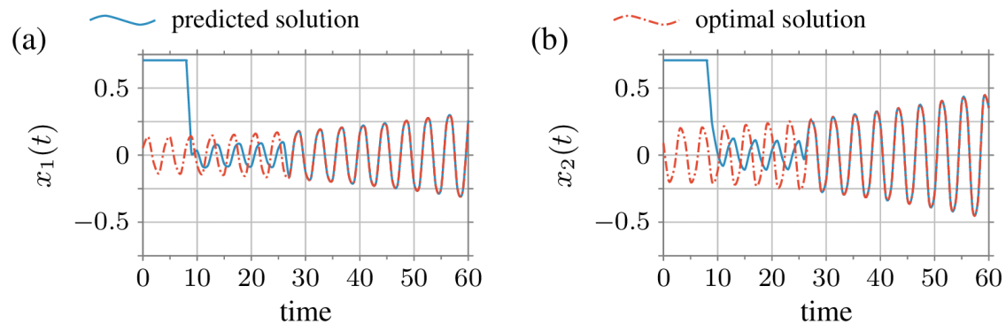
Figure 1: This figure shows the predicted (solid blue line) and the optimal solution (dashed red line) considering a quadratic cost function for the setting described in Section IV-A as a function of time. Panels (a) and (b) shows the evolution of the first and the second component of the predicted and the optimal solution, respectively. The data $X_{0}$ and $Y_{0}$ in (4) are collected when $t\!\in\![0,8]$, where $[x_{1}(t),x_{2}(t)]^{\mathsf{T}}=[\sqrt{2}/2,\sqrt{2}/2]^{\mathsf{T}}$ and the data $X_{1}$ and $Y_{1}$ in (4) are collected when $t\!\in\![9,26]$, where $x(t)$ is obtained using static gradient descent (24). For $t>26$, we predict the optimal solution using (23). We observe that the predicted value converges to the optimal solution for $t>26$.

We estimate the realization of the system dynamics $A$ (using $x(t)=[\sqrt{2}/2,\sqrt{2}/2]^{\mathsf{T}}$ for $t\in[0,N_{0}]$), up to similarity transformation, using the collected data structured in the Hankel matrix form as in (6). Specifically, we compute $\bar{A}$ using (9) and then propagate $\bar{A}$ to obtain $[\bar{z}(N_{0}+1),\cdots,\bar{z}(N)]=\bar{A}^{p}[\bar{z}(p-1),\cdots,\bar{A}^{N-2p+1}\bar{z}(p-1)]$, where $\bar{z}(p-1)$ is computed from (10). Then, from Theorems III.1 and III.2, we have a full rank matrix $M$, which is constructed as in (11). Using (12), we can compute the transformation matrix $T$ that transforms the realization $\bar{A}$ to $A$ and $\bar{z}(t)$ to the coordinate of $z(t)$ for $t\geq 0$.

Using the estimated $A$, we predict the evolution of $z(t)$ and compute a solution to the optimization problem as

$$x(t)=-\underbrace{\begin{bmatrix}h_{11}(t)&h_{12}(t)\\ h_{12}(t)&h_{22}(t)\end{bmatrix}^{-1}}_{H(t)^{-1}}\begin{bmatrix}b_{1}(t)\\ b_{2}(t)\end{bmatrix}.$$ (23)

Fig. 1 shows the predicted and the optimal solution over time for the quadratic optimization. For comparison, we use a static gradient descent algorithm that does not take into account the time-varying nature of the cost function and updates the solution to the optimization problem as

$$x(t)=x(t-1)-\eta y(x(t-1),t-1),$$ (24)

for $t\in[N_{0}+1,N]$, with $\eta=10^{-3}$, with $x(0)=[\sqrt{2}/2,\sqrt{2}/2]^{\mathsf{T}}$. As can be seen in Fig. 2(a), our methods converges to the optimal solution in finite time, whereas the static gradient descent algorithm does not converge to the optimal solution.

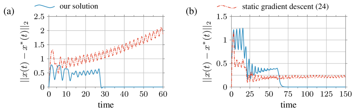
Figure 2: The figure shows a comparison of our proposed solution (solid blue line) with the static gradient descent algorithm (24) (dashed red line). Panel (a) and (b) shows the error in estimating the optimal solution for a quadratic cost function and a higher order polynomial, respectively. We observe that the error decays to zero for $t>N$ using our solution proposed in Section IV-A and IV-B. However, for the static gradient descent (24), we observe that the error diverges.

IV-B Time-varying polynomial optimization

We consider now a third-order polynomial with time-varying coefficients as

$$f(x,z(t))=\sum_{r=1}^{3}\underbrace{\begin{bmatrix}x^{\mathsf{T}}\otimes\cdots\otimes x^{\mathsf{T}}\end{bmatrix}}_{\text{r-terms}}z(t),$$ (25)

where $x\in\mathbb{R}^{2}$, and $z(t)=[z_{1}(t)^{\mathsf{T}},z_{2}(t)^{\mathsf{T}},z_{3}(t)^{\mathsf{T}}]^{\mathsf{T}}$, with $z_{r}(t)\in\mathbb{R}^{2^{r}}$ for $r\in\{1,2,3\}$ representing the vector of coefficients. The dynamics of $z(t)$ follow (2) with $A:=\mathrm{blkdiag}([M_{1},M_{2},M_{3}])$, $M_{1}=\begin{bmatrix}0&1\\ -1&0\end{bmatrix}$, $M_{2}=\operatorname{diag}[0.98,0.99,0.99,0.95]$ and $M_{3}=\operatorname{diag}[0.88,0.87,0.87,0.89,0.87,0.89,0.89,0.85]$. We start from $z_{1}(0)=[-63.7,110.2]^{\mathsf{T}}$, $z_{2}(0)=\begin{bmatrix}2.23,2.46,2.46,6.24\end{bmatrix}^{\mathsf{T}}$ and $z_{3}(0)=[0.5,0.3,0.3,0.4,0.3,0.4,0.4,0.6]^{\mathsf{T}}$. The gradient of (25) is

$$y(x,t)=\begin{bmatrix}P_{1}(x)&P_{2}(x)&P_{3}(x)\end{bmatrix}z(t),$$

where $P_{1}(x)=I_{2},P_{2}(x)=(x^{\mathsf{T}}\otimes I_{2}+I_{2}\otimes x^{\mathsf{T}})$, and $P_{3}(x)=(x^{\mathsf{T}}\otimes x^{\mathsf{T}}\otimes I_{2}+x^{\mathsf{T}}\otimes I_{2}\otimes x^{\mathsf{T}}+I_{2}\otimes x^{\mathsf{T}}\otimes x^{\mathsf{T}})$. We use $N_{0}=18$ and $N=60$ for the data collection as in (4).

Unlike the case of quadratic cost function, a closed form expression of the solution to the optimization problem is not available for higher order polynomials. Instead, we employ a time-varying gradient descent algorithm as in Algorithm 1, updating the solution based on the parameter $z(t)$. We set the algorithm parameters as $\beta=10^{-2}$, $D=500$, and $T=150$. Fig. 3 shows the predicted and the optimal solution for a higher order polynomial. We observe in Fig. 3 that the predicted solution attempts to track the optimal solution for $t\in[N_{0}+1,N]$ but never converges to it when computed via (24). We also observe that the predicted value converges to the optimal solution for $t>N$. Finally, Fig. 2(b) shows a comparison of the proposed algorithm and the gradient descent algorithm using (24). As expected, our method converges to the optimal solution (up to the convergence of the gradient descent algorithm), whereas the static optimization algorithm (24) does not converge.

Require: initial condition $x(N)$, step size $\beta$

for $t=N,N+1,\ldots,T$ do

    Obtain $z(t)$ using $A$ and $z(0)$

    Initialize $x_{0}(t)=x(t)$

    for $d=0,1,\ldots,D-1$ do

       ​​$x_{d+1}(t)\!=\!x_{d}(t)\!-\!\beta\nabla_{x}f(x_{d}(t);z(t))$

    end for

   Set $x(t+1)=x_{D}(t)$

end for

Algorithm 1 Time-varying gradient descent [24]

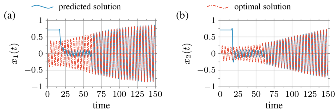
Figure 3: This figure shows the predicted (solid blue line) and the optimal solution (dashed red line) considering a third-order polynomial cost function for the setting described in Section IV-B as a function of time. Panels (a) and (b) shows the evolution of the first and the second component of the predicted and the optimal solution, respectively.The data $X_{0}$ and $Y_{0}$ in (4) are collected when $t\!\in\![0,18]$, where $[x_{1}(t),x_{2}(t)]^{\mathsf{T}}=[\sqrt{2}/2,\sqrt{2}/2]^{\mathsf{T}}$ and the data $X_{1}$ and $Y_{1}$ in (4) are collected when $t\!\in\![19,60]$, where $x(t)$ is obtained using (24). For $t>26$, we predict the optimal solution using algorithm 1. We observe that the predicted value converges to the optimal solution for $t>60$.

IV-C Non-polynomial function

In this section, we discuss the application of the proposed algorithm to a non-polynomial problem. In particular, we consider the following cost function:

$$f(x,z(t))=\begin{bmatrix}2e^{x}&\sin x&x\end{bmatrix}z(t),$$ (26)

where $f:\mathbb{R}\times\mathbb{R}^{3}\rightarrow\mathbb{R}$, and $z(t)=[\theta_{1}(t),\theta_{2}(t),\theta_{3}(t)]^{\mathsf{T}}$ is a time varying parameter. The dynamics of $z(t)$ is given by (2) with $A=\operatorname{diag}([0.99,0.97,0.98])$. The gradient of (26) is

$$y(x,t)=\begin{bmatrix}2e^{x}&\cos x&1\end{bmatrix}z(t).$$

We collect the data as in (4), with $x(t)=x_{0}=0.7$ for $t\in[0,6]$ and for $t\in[7,30]$ we compute $x(t)$ using (24) with $\eta=10^{-3}$. Using the collected data, we estimate the parameters $A$ and $z(t)$ for $t\geq 0$, following our methodology as in the previous examples. Once $A$ is estimated, we predict the evolution of $z(t)$ and compute a solution using Algorithm 1 with parameters $\beta=10^{-2}$, $D=500$, and $T=150$. Fig. 4(a) shows the predicted and the optimal solution for the cost function in (26) and Fig. 4(b) compares the performance of our solution using algorithm 1 with the static gradient descent algorithm, as described in (24).

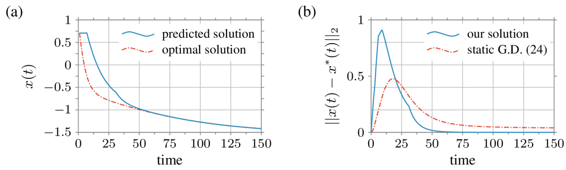
Figure 4: The figure in panel (a) shows the predicted (solid blue line) and the optimal solution (dashed red line) considering a non-polynomial cost function for the setting described in Section IV-C as a function of time. The data $X_{0}$ and $Y_{0}$ in (4) are collected when $t\!\in\![0,6]$, where $[x_{1}(t),x_{2}(t)]^{\mathsf{T}}=[\sqrt{2}/2,\sqrt{2}/2]^{\mathsf{T}}$ and the data $X_{1}$ and $Y_{1}$ in (4) are collected when $t\!\in\![7,30]$, where $x(t)$ is obtained using (24). For $t>26$, we predict the optimal solution using algorithm 1. The figure in panel (b) shows the error in computing the optimal solution, using our solution (solid blue line) and static gradient descent (24) (dashed red line). We observe that unlike the static gradient descent algorithm (24), the predicted value converges to the optimal solution using our proposed solution.

V Conclusion

In this work we study online time-varying optimization with unknown, time-varying parameters, where gradient measurements are leveraged to learn these parameters. We show how system identification techniques can be used to estimate the parameters in their exact coordinates through a transformation matrix. We also establish necessary and sufficient conditions for computing the transformation matrix, ensuring accurate parameter reconstruction. An open question in our ongoing research is whether our approach can be extended to a more general class of cost functions. For a general cost function, the dynamics would be non-linear and time-varying. Exploring the robustness of our method in noisy environments or including constrains in our cost function are also important areas of future investigation.

E-A Technical lemmas

Lemma E-A.1.

(Null-space of Kronecker product) Let $A\in\mathbb{R}^{n\times m}$ and $B\in\mathbb{R}^{l\times k}$. Then,

$$\text{Ker}\left(A\otimes B\right)=\text{Ker}\left(A\otimes I_{k}\right)\cup\text{Ker}\left(I_{m}\otimes B\right).$$

Proof:

From [25, Fact 7.4.23], we have

$$\text{Im}\left(A^{\mathsf{T}}\otimes B^{\mathsf{T}}\right)=\text{Im}\left(A^{\mathsf{T}}\otimes I_{k}\right)\cap\text{Im}\left(I_{m}\otimes B^{\mathsf{T}}\right).$$

The orthogonal complement of $\text{Im}\left(A^{\mathsf{T}}\otimes B^{\mathsf{T}}\right)$ is written as

$$\text{Im}\left(A^{\mathsf{T}}\otimes B^{\mathsf{T}}\right)^{\perp}=\text{Im}\left(A^{\mathsf{T}}\otimes I_{k}\right)^{\perp}\cup\text{Im}\left(I_{m}\otimes B^{\mathsf{T}}\right)^{\perp}.$$

The proof follows by noting that $\text{Im}\left(X\right)^{\perp}=\text{Ker}\left(X^{\mathsf{T}}\right)$ for any matrix $X$. ∎

Lemma E-A.2.

(Basis of the null-space of Kronecker product) Let $A\in\mathbb{R}^{n\times m}$ with $\operatorname{Rank}{\left(A\right)}=r$. Let $K\in\mathbb{R}^{m\times(m-r)}$ be a matrix whose columns span $\text{Ker}\left(A\right)$. Then, the columns of $K\otimes I_{k}$ span $\text{Ker}\left(A\otimes I_{k}\right)$.

Proof:

We begin by noting that $\operatorname{Col}{\left(K\otimes I_{k}\right)}\!\in\!\text{Ker}\left(A\otimes I_{k}\right)$ since $\left(A\otimes I_{k}\right)\left(K\otimes I_{k}\right)\!=\!AK\otimes I_{k}\!=\!0$. Thus, the proof boils down to showing that $\operatorname{Rank}{\left(K\otimes I_{k}\right)}\!=\!\dim{\left(\text{Ker}\left(A\otimes I_{k}\right)\right)}$. Using [25, Fact 7.4.24], we have $\operatorname{Rank}{\left(A\otimes I_{k}\right)}\!=\!rk$. Consequently, using the rank-nullity theorem, we have, $\dim{\left(\text{Ker}\left(A\otimes I_{k}\right)\right)}\!=\!mk\!-\!rk$. Further, since $\operatorname{Rank}{\left(K\right)}\!=\!m-r$, using [25, Fact 7.4.24] we have, $\operatorname{Rank}{\left(K\otimes I_{k}\right)\!=\!mk-rk}\!=\!\dim{\left(\text{Ker}\left(A\otimes I_{k}\right)\right)}$. Therefore, the columns of $K\otimes I_{k}$ span $\text{Ker}\left(A\otimes I_{k}\right)$. ∎

References

- [1] P. M. Wensing, M. Posa, Y. Hu, A. Escande, N. Mansard, and A. Del Prete. Optimization-based control for dynamic legged robots. IEEE Transactions on Robotics, 40:43–63, 2024.
- [2] D. P. Bertsekas. Dynamic Programming and Optimal Control, volume 2. Athena Scientific, 4 edition, 2018.
- [3] C. M. Bishop. Pattern recognition and machine learning, volume 4. Springer, 4 edition, 2006.
- [4] B. T. Polyak. Introduction to optimization. New York, Optimization Software,, 1987.
- [5] A. Simonetto, E. Dall’Anese, S. Paternain, G. Leus, and G. B. Giannakis. Time-varying convex optimization: Time-structured algorithms and applications. Proceedings of the IEEE, 108(11):2032–2048, 2020.
- [6] S. Shalev-Shwartz. Online learning and online convex optimization. Foundations and Trends® in Machine Learning, 4(2):107–194, 2012.
- [7] E. C. Hall and R. M. Willett. Online convex optimization in dynamic environments. IEEE Journal of Selected Topics in Signal Processing, 9(4):647–662, 2015.
- [8] R. Dixit, A. S. Bedi, R. Tripathi, and K. Rajawat. Online learning with inexact proximal online gradient descent algorithms. IEEE Transactions on Signal Processing, 67(5):1338–1352, 2019.
- [9] S. M. Fosson. Centralized and distributed online learning for sparse time-varying optimization. IEEE Transactions on Automatic Control, 66(6):2542–2557, 2020.
- [10] E. Dall’Anese, A. Simonetto, S. Becker, and L. Madden. Optimization and learning with information streams: Time-varying algorithms and applications. IEEE Signal Processing Magazine, 37(3):71–83, 2020.
- [11] P. Cisneros-Velarde, S. Jafarpour, and F. Bullo. A contraction analysis of primal-dual dynamics in distributed and time-varying implementations. IEEE Transactions on Automatic Control, 67(7):3560–3566, 2022.
- [12] A. Davydov, V. Centorrino, A. Gokhale, G. Russo, and F. Bullo. Contracting dynamics for time-varying convex optimization. arXiv preprint arXiv:2305.15595, 2023.
- [13] M. Baumann, C. Lageman, and U. Helmke. Newton-type algorithms for time-varying pose estimation. Intelligent Sensors, Sensor Networks and Information Processing Conference, 2004., pages 155–160, Melbourne, VIC, Australia, Dec. 2004.
- [14] S. Rahili and W. Ren. Distributed continuous-time convex optimization with time-varying cost functions. IEEE Transactions on Automatic Control, 62(4):1590–1605, 2016.
- [15] M. Fazlyab, S. Paternain, V. M. Preciado, and A. Ribeiro. Prediction-correction interior-point method for time-varying convex optimization. IEEE Transactions on Automatic Control, 63(7):1973–1986, 2017.
- [16] A. Simonetto, A. Mokhtari, A. Koppel, G. Leus, and A. Ribeiro. A class of prediction-correction methods for time-varying convex optimization. IEEE Transactions on Signal Processing, 64(17):4576–4591, 2016.
- [17] A. Simonetto and E. Dall’Anese. Prediction-correction algorithms for time-varying constrained optimization. IEEE Transactions on Signal Processing, 65(20):5481–5494, 2017.
- [18] A. Simonetto. Dual prediction–correction methods for linearly constrained time-varying convex programs. IEEE Transactions on Automatic Control, 64(8):3355–3361, 2018.
- [19] N. Bastianello, R. Carli, and S. Zampieri. Internal model-based online optimization. IEEE Transactions on Automatic Control, 69(1):689–696, 2024.
- [20] U. Casti, N. Bastianello, R. Carli, and S. Zampieri. A control theoretical approach to online constrained optimization. arXiv preprint arXiv:2309.15498, 2024.
- [21] G. Bianchin and B. V. Scoy. The internal model principle of time-varying optimization. arXiv preprint arXiv:2407.08037, 2024.
- [22] G. Bianchin and B. V. Scoy. The Discrete-time Internal Model Principle of Time-varying Optimization: Limitations and Algorithm Design. 2024.
- [23] S. Y. Kung. A new identification and model reduction algorithm via singular value decomposition. Asilomar Conf. on Circuits, Systems and Computer, pages 705–714, 1978.
- [24] H. Iwakiri, T. Kamijima, S. Ito and A. Takeda. Prediction-Correction Algorithm for Time-Varying Smooth Non-Convex Optimization. arXiv preprint arXiv:2402.06181, 2024.
- [25] D. S. Bernstein. Matrix Mathematics. Princeton University Press, 2 edition, 2009.