Temporal-Consistent Video Restoration with Pre-trained Diffusion Models

Abstract

Video restoration (VR) aims to recover high-quality videos from degraded ones. Although recent zero-shot VR methods using pre-trained diffusion models (DMs) show good promise, they suffer from approximation errors during reverse diffusion and insufficient temporal consistency. Moreover, dealing with 3D video data, VR is inherently computationally intensive. In this paper, we advocate viewing the reverse process in DMs as a function and present a novel Maximum a Posterior (MAP) framework that directly parameterizes video frames in the seed space of DMs, eliminating approximation errors. We also introduce strategies to promote bilevel temporal consistency: semantic consistency by leveraging clustering structures in the seed space, and pixel-level consistency by progressive warping with optical flow refinements. Extensive experiments on multiple virtual reality tasks demonstrate superior visual quality and temporal consistency achieved by our method compared to the state-of-the-art.

1 Introduction

Figure 1: Visualization of sample VR results by our method: (a) Super-resolution $\times 4$; (b) Inpainting with $50\%$ random pixel masking; (c) Temporal deconvolution using uniform PSF with kernel width $k=7$; and (d) Temporal deconvolution with motion deblurring.

Video restoration (VR) aims to recover high-quality (HQ) videos $\mathbf{X}$ from given low-quality (LQ) observations $\mathbf{Y}\approx\mathcal{A}\pqty{\mathbf{X}}$, where $\mathcal{A}$ represents a spatial and/or temporal degradation. Typical VR tasks include super-resolution [1, 2, 3, 4], inpainting [5, 6, 7], and deblurring [8, 9].

Modern VR methods rely on deep learning and fall into two main categories. (1) The supervised learning approach trains deep neural networks (DNNs) on LQ-HQ paired data, i.e., $\{(\mathbf{Y}_{i},\mathbf{X}_{i})\}_{i=1}^{K}$, to learn direct mappings from $\mathbf{Y}$ to $\mathbf{X}$. Although conceptually simple, these methods require large-scale, high-quality paired datasets and significant computational resources (e.g. 32 A100-80G GPUs for super-resolution [1]). Moreover, they need to train new DNNs for different VR tasks, with limited task adaptability; (2) The zero-shot paradigm enabled by pre-trained deep generative models, especially diffusion models (DMs) [10, 11]. Due to the lack of mature video DMs, recent research [12, 13, 14, 15] has adopted pre-trained image DMs for VR, achieving remarkable results without task-specific retraining.

Most zero-shot DM-based VR methods [14, 13, 15, 12] interleave reverse diffusion steps with iterative gradient updates or projections to approach the feasible set $\{\mathbf{X}\mid\mathbf{Y}\approx\mathcal{A}(\mathbf{X})\}$. However, these methods usually face three fundamental challenges. First, they suffer from unavoidable approximation errors (Challenge 1) when approximating an intractable likelihood [16], regardless of whether they employ gradient updates or projections. These errors accumulate throughout the reverse diffusion process, potentially degrading the reconstruction quality. Second, these zero-shot methods often struggle for satisfactory temporal consistency (Challenge 2) due to the difficulty in extracting accurate motion information from LQ measurements and the absence of explicit motion priors in the image DMs they leverage. Third, compared to image restoration, VR entails significantly more computation and memory footprints (Challenge 3), creating substantial efficiency barriers that must be addressed for practical applications.

In this paper, we focus on solving video restoration (VR) problems using pre-trained image DMs, while addressing the three fundamental challenges faced by state-of-the-art (SOTA) methods. We specifically choose latent diffusion models (LDMs) as our backbone DMs due to their superior generation quality, computational efficiency, and widespread adoption. (Tackling Challenge 1) Our method builds upon the classical Maximum a Posterior (MAP) framework [17, 18, 19, 20, 21, 22]:

$$\min_{\mathbf{X}}\ \;\underbrace{\ell\pqty{\mathbf{Y},\mathcal{A}\pqty{\mathbf{X}}}}_{\text{data consistency}}+\lambda\underbrace{\Omega\pqty{\mathbf{X}}}_{\text{regularization}}.$$ (1)

We take a novel perspective that views the entire reverse diffusion process as a function $\mathcal{R}$ which, when composed with the pre-trained decoder $\mathcal{D}$ in LDMs, maps from the seed space directly to the image manifold $\mathcal{M}$. This allows us to naturally reparameterize the video frame-by-frame as $\mathbf{X}=[\mathcal{D}\circ\mathcal{R}\pqty{\mathbf{z}_{1}},\dots,\mathcal{D}\circ\mathcal{R}\pqty{\mathbf{z}_{N}}]$; plugging this into Eq.˜1 leads to a unified optimization formulation with respect to the seeds $\mathbf{Z}=[\mathbf{z}_{1},\dots,\mathbf{z}_{N}]$. This reparametrization approach effectively leverages the powerful LDM priors for VR while avoiding the approximation errors inherent in SOTA methods. To address Challenge 2, we design a hierarchical framework to promote bilevel temporal consistency. For semantic-level temporal consistency, we first explore the seed space and observe an intriguing clustering phenomenon: input seeds of frames from different videos are scattered, while those of frames within the same video are clustered. Motivated by this, we construct a noise prior by hypothesizing that consecutive frames share a common seed with only minor frame-specific variations. To enhance pixel-level temporal consistency, we implement a progressive warping mechanism that combines image warping with incremental optical flow (OF) refinements. Our ablation study in Tab.˜7 underscores the effectiveness of both components in enhancing bilevel temporal consistency. To deal with Challenge 3, we introduce an efficient diffusion sampling strategy using the DDIM sampler. Notably, our ablation study (Tab.˜1) reveals that $4$ reverse steps in $\mathcal{R}$ are sufficient to achieve the SOTA performance. Moreover, by leveraging the multivariate mean value theorem, we significantly reduce the computational complexity of the proposed method. To further boost efficiency, we make the trainable residuals for each frame more lightweight through low-rank approximations. Our contributions can be summarized as follows:

• We propose a MAP-based framework for VR that harnesses pre-trained image DMs by reparameterizing frames via the entire reverse diffusion process, eliminating the approximation errors that have plagued SOTA methods.

• We devise a compelling hierarchical approach for bilevel temporal consistency that unites semantic-level coherence (through our key discovery of clustering patterns in the seed space) with pixel-level precision (via dynamic progressive warping with optical flow refinements).

• We design our method with exceptional computational efficiency through three innovations: an optimized DDIM sampling strategy that requires only $4$ steps, an approximate reformulation using the multivariate mean value theorem, and memory-efficient trainable residuals with low-rank approximations.

• Our comprehensive experiments on challenging VR tasks demonstrate that our method leads to substantial performance improvements over SOTA methods, providing exceptional visual quality and temporal consistency.

2 Background and related work

Diffusion models (DMs)

Recently, DMs have dominated generative models, capable of producing high-quality objects. The early denoising diffusion probabilistic model (DDPM) [10] involves two processes: a forward diffusion process that transforms any clean data sample $\mathbf{x}_{0}\sim p_{\text{data}}$ into pure noise $\mathbf{x}_{T}\sim\mathcal{N}\pqty{\mathbf{0},\mathbf{I}}$ by sequential noise injection, governed by the stochastic differential equation (SDE): $d\mathbf{x}=-\beta_{t}/2\cdot\mathbf{x}dt+\sqrt{\beta_{t}}d\mathbf{w}$, where $\beta_{t}$ represents the noise schedule, and $\mathbf{w}$ denotes the standard Wiener process; a reverse diffusion process that performs sequential denoising, turning any seed noise into a useful data sample—hence responsible for data generation, and follows the form:

$$d\mathbf{x}=-\beta_{t}\left[\mathbf{x}/2+\nabla_{\mathbf{x}}\log p_{t}(\mathbf{x})\right]dt+\sqrt{\beta_{t}}d\overline{\mathbf{w}},$$ (2)

where $\overline{\mathbf{w}}$ is the time-reversed Brownian motion, and the term $\nabla_{\mathbf{x}}\log p_{t}(\mathbf{x})$, known as the score function, represents the gradient of the log-likelihood. To train an DM, this score function is approximated using a DNN, $\mathbf{\varepsilon}_{\mathbf{\theta}}^{(t)}\pqty{\mathbf{x}}$, trained via score matching techniques [23, 24]. In practice, the diffusion process is discretized in $T$ time steps, using a predefined variance schedule $\beta_{1},\dots,\beta_{T}$. Defining $\alpha_{t}\doteq 1-\beta_{t}$ with $\alpha_{T}\to 0$ and $\bar{\alpha}_{t}\doteq\prod_{s=1}^{t}\alpha_{s}$, the forward steps are written as: $\mathbf{x}_{t}=\sqrt{1-\beta_{t}}\mathbf{x}_{t-1}+\sqrt{\beta_{t}}\mathbf{z}$, where $\mathbf{z}\sim\mathcal{N}\pqty{\mathbf{0},\mathbf{I}}$. The reverse steps run as $\mathbf{x}_{t-1}=1/\sqrt{\alpha_{t}}\cdot\left(\mathbf{x}_{t}-\beta_{t}\mathbf{\varepsilon}_{\mathbf{\theta}}^{(t)}(\mathbf{x}_{t})/\sqrt{1-\bar{\alpha}_{t}}\right)+\sqrt{\beta_{t}}\mathbf{z}$; this iterative sampling process usually requires a large number of steps to achieve high-quality generation, leading to slow inference. To address this slowness, the denoising diffusion implicit model (DDIM) [11] introduces a non-Markovian relaxation of the forward process, allowing each step $\mathbf{x}_{t}$ to depend not only on $\mathbf{x}_{t-1}$ but also directly on $\mathbf{x}_{0}$. This relaxation enables sampling with fewer steps while maintaining generation quality. The reverse step in DDIM is

$$\mathbf{x}_{t-1}=\sqrt{\bar{\alpha}_{t-1}}\widehat{\mathbf{x}}_{0}\pqty{\mathbf{x}_{t}}+\sqrt{1-\bar{\alpha}_{t-1}}\mathbf{\varepsilon}_{\mathbf{\theta}}^{(t)}(\mathbf{x}_{t}),$$ (3)

where $\widehat{\mathbf{x}}_{0}\pqty{\mathbf{x}_{t}}\doteq(\mathbf{x}_{t}-\sqrt{1-\bar{\alpha}_{t}}\mathbf{\varepsilon}_{\mathbf{\theta}}^{(t)}(\mathbf{x}_{t}))/\sqrt{\bar{\alpha}_{t}}$ estimates the clean image $\mathbf{x}_{0}$ from $\mathbf{x}_{t}$.

Despite DDIM’s speedup, training diffusion models in high-resolution pixel spaces remains computationally expensive. Latent diffusion models (LDMs) [25] overcome this by performing both training and inference in low-dimensional latent spaces, wrapped into pre-trained encoder-decoder models. The LDM framework has become dominant in SOTA visual generative models [25, 26, 27].

DMs for video restoration

Approaches to VR using DMs can be categorized into two main classes: supervised [28, 1] and zero-shot [14, 15, 13, 12]. Supervised methods train DM-based models on paired data or correlated noise, which is outside our focus (see discussion Sec.˜1). Zero-shot methods largely inherit ideas from zero-shot image restoration with pre-trained DMs and most of them focus on directly modeling the conditional distribution $p_{t}(\mathbf{x}|\mathbf{y})$ and substitute the unconditional score function $\nabla_{\mathbf{x}}\log p_{t}(\mathbf{x})$ in Eq.˜2 with the conditional score function $\nabla_{\mathbf{x}}\log p_{t}(\mathbf{x}|\mathbf{y})=\nabla_{\mathbf{x}}\log p_{t}(\mathbf{x})+\nabla_{\mathbf{x}}\log p_{t}(\mathbf{y}|\mathbf{x})$, i.e.,

$$d\mathbf{x}=-\beta_{t}\left[\mathbf{x}/2+\pqty{\nabla_{\mathbf{x}}\log p_{t}(\mathbf{x})+\nabla_{\mathbf{x}}\log p_{t}(\mathbf{y}|\mathbf{x})}\right]dt\\ +\sqrt{\beta_{t}}d\overline{\mathbf{w}}.$$ (4)

Here, while $\nabla_{\mathbf{x}}\log p_{t}(\mathbf{x})$ can be approximated using the pre-trained score function $\mathbf{\varepsilon}_{\mathbf{\theta}}^{(t)}\pqty{\mathbf{x}}$, the term $\nabla_{\mathbf{x}}\log p_{t}(\mathbf{y}|\mathbf{x})$ remains intractable because $\mathbf{y}$ does not depend directly on $\mathbf{x}(t)$. To circumvent this, one line of research directly approximates $p_{t}(\mathbf{y}|\mathbf{x}(t))$ [16, 29], while the other interleaves diffusion reverse steps from Eq.˜3 with projections (or gradient updates) [30] to guide the process toward the feasible set $\{\mathbf{x}|\mathbf{y}\approx\mathcal{A}\pqty{\mathbf{x}}\}$. Unfortunately, both strategies introduce unavoidable approximation errors (Challenge 1) that can accumulate during the reverse diffusion process (RDP), ultimately limiting their practical performance. For VR, [13] follows the generative diffusion prior (GDP) framework [29] using gradient steps, while [14, 15] implement the decomposed diffusion sampling (DDS) [30] approach with several conjugate gradient (CG) update steps. However, CG requires the degradation operator $\mathcal{A}$ to be known, symmetric and positive-definite [31], restricting its applicability for VR.

VR also needs good temporal consistencies. To address this issue, existing zero-shot methods use batch-consistent sampling strategies [14, 15] and leverage optical flow (OF) guidance. However, accurate OF estimation from LQ videos is inherently challenging. Different approaches attempt to overcome this limitation: [12] directly obtains OF from LQ videos and proposes a hierarchical latent warping technique, while [13] acquires OFs during intermediate stages of the RDP—when results may still contain noise—and applies these OFs for warping in the image space. In summary, the SOTA methods achieve only semantic-level alignment [14, 15, 12] or attempt pixel-level alignment with suboptimal OFs [13], leaving temporal consistency in VR a critical standing challenge (Challenge 2).

3 Our method

In this paper, we employ pre-trained image LDMs as priors to solve video restoration (VR) problems due to their superior generation quality, computational efficiency, and widespread adoption. In Sec.˜3.1, we propose a novel LDM-based formulation that overcomes the limitations of SOTA methods, addressing challenge 1. In Sec.˜3.2, we introduce two effective components for bilevel temporal consistency, tackling challenge 2. Finally, in Sec.˜3.3, we present several essential techniques to ensure computational and memory efficiency, targeting challenge 3.

3.1 Our basic formulation

To mitigate approximation errors in existing interleaving methods, we introduce a novel and principled formulation for solving VR problems following the classical maximum a posteriori (MAP) principle. Our goal is to recover a high-quality video $\mathbf{X}$ that not only satisfies the measurement constraint $\mathbf{Y}\approx\mathcal{A}(\mathbf{X})$, but also resides near the realistic video manifold $\mathcal{M}$: $\min_{\mathbf{X}\in\mathcal{M}}\ \;\ell\pqty{\mathbf{Y},\mathcal{A}\pqty{\mathbf{X}}}$. Inspired by [22], we propose viewing the entire RDP as a function $\mathcal{R}$, which, when composed with the pre-trained decoder $\mathcal{D}$ in LDMs, maps the seed space to the video space. This fresh perspective enables us to reparameterize the video as $\mathbf{X}=\mathcal{D}\circ\mathcal{R}(\mathbf{Z})$, which can then be plugged into the MAP framework Eq.˜1, leading to a unified formulation:

$$\mathbf{Z}^{*}\in\min\nolimits_{\mathbf{Z}}\;\ell\pqty{\mathbf{Y},\mathcal{A}\pqty{\mathcal{D}\circ\mathcal{R}\pqty{\mathbf{Z}}}},$$ (5)

where $\mathbf{Z}=[\mathbf{z}_{1},\dots,\mathbf{z}_{N}]$, and $\mathcal{D}$ and $\mathcal{R}$ are applied framewise. The final reconstruction can be obtained as $\mathbf{X}^{*}=\mathcal{D}\circ\mathcal{R}(\mathbf{Z}^{*})$. Note that the RDP consists of multiple iterative steps. Mathematically, a single reverse step can be expressed as a function $g$ that depends on $\mathbf{\varepsilon}_{\mathbf{\theta}}^{(i)}$, i.e., $g_{\mathbf{\varepsilon}_{\mathbf{\theta}}^{(i)}}$, representing the $i$-th reverse step that maps the latent variable $\mathbf{z}_{i+1}$ to $\mathbf{z}_{i}$. The full RDP can then be written as

$$\mathcal{R}\doteq g_{\mathbf{\varepsilon}_{\mathbf{\theta}}^{(0)}}\circ g_{\mathbf{\varepsilon}_{\mathbf{\theta}}^{(1)}}\circ\cdots\circ g_{\mathbf{\varepsilon}_{\mathbf{\theta}}^{(T-2)}}\circ g_{\mathbf{\varepsilon}_{\mathbf{\theta}}^{(T-1)}}.$$ (6)

3.2 Promoting bilevel temporal consistency

Although our formulation in Eq.˜5 can address VR tasks leveraging pre-trained image LDMs, the reconstructed videos still may not have good temporal consistency (see “Base” in Tab.˜7). This is not surprising, as it tries to recover individual frames separately and fails to capture inter-frame dependencies—a critical issue to be addressed by all methods relying on image DMs [13, 14, 15, 12]. In this section, we address this critical issue (Tackling Challenge 2) by introducing two distinct components that target temporal consistency at two different levels.

3.2.1 Noise prior for semantic-level consistency

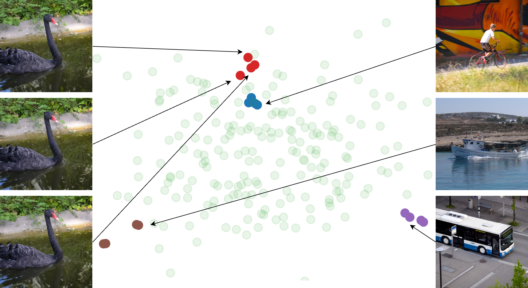
Figure 2: T-SNE [32] visualization of seeds extracted for video frames. Green dots are i.i.d. Gaussian noise. Seeds for the same video form clusters, while those for different videos are scattered.

An intriguing clustering phenomenon

To strengthen temporal consistency, we begin by exploring potential structures in the seed space. We obtain seeds $\mathbf{Z}$ for randomly sampled frames from videos by solving the regression problem: $\min\nolimits_{\mathbf{Z}}\;\ell\pqty{\mathbf{X},\mathcal{D}\circ\mathcal{R}(\mathbf{Z})}$. From Fig.˜2, we observe an interesting pattern: seeds for frames of different videos are widely scattered without apparent correlation, whereas seeds for frames of the same video tend to cluster together—a pattern we can potentially leverage to improve temporal consistency across frames.

To this end, we hypothesize that consecutive frames share a common seed but have minor frame-specific deviations. Accordingly, we decompose the seed matrix as $\mathbf{Z}=\mathbf{z}_{shared}\mathbb{1}^{\intercal}+\mathbf{R}$, where $\mathbf{z}_{shared}$ represents the shared seed, $\mathbf{R}=[\mathbf{r}_{1},\dots,\mathbf{r}_{N}]$ captures frame-specific residuals, and $\mathbb{1}$ is an all-one vector. Moreover, we need to ensure that the residuals are small by constraining $\|\mathbf{r}_{i}\|_{2}\leq\sigma$ for a small constant $\sigma>0$. Our new formulation built on Eq.˜5 is

$$\begin{split}\min\nolimits_{\mathbf{z}_{shared},\mathbf{R}}&\quad\ell\pqty{\mathbf{Y},\mathcal{A}\pqty{\mathcal{D}\circ{\mathcal{R}\pqty{\mathbf{z}_{shared}\mathbb{1}^{\intercal}+\mathbf{R}}}}},\\ \text{s.t.}&\quad\|\mathbf{r}_{i}\|_{2}\leq\sigma,\quad\forall i\in\{1,\ldots,N\},\end{split}$$ (7)

where $\mathcal{D}$ and $\mathcal{R}$ are applied framewise. To solve this constrained optimization problem, we choose the Projected Gradient Descent (PGD) method. Our algorithm alternates between gradient descent and projection:

$$\begin{split}(\mathbf{z}_{shared},\mathbf{R})&\leftarrow(\mathbf{z}_{shared},\mathbf{R})-\eta\nabla_{(\mathbf{z}_{shared},\mathbf{R})}\ell,\\ \mathbf{r}_{i}&\leftarrow\Pi_{\|\mathbf{r}_{i}\|_{2}\leq\sigma}(\mathbf{r}_{i}),\quad\forall i\in\{1,\ldots,N\}.\end{split}$$ (8)

Here, $\Pi_{\|\mathbf{r}_{i}\|_{2}\leq\sigma}$ denotes the projection operator that maps $\mathbf{r}_{i}$ to the closest point within the $\ell_{2}$ norm ball of radius $\sigma$.

3.2.2 Progressive warping for pixel-level consistency

As shown in Tab.˜7, incorporating the noise prior improves both data fidelity and temporal consistency. However, fine-grained consistency across frames remains weak. To enhance it, we introduce a progressive warping loss:

$$\mathcal{L}_{\text{warp}}=\sum\nolimits_{n=1}^{N-1}\ell\left(\mathbf{M}\odot\mathbf{x}^{\prime}_{n},\mathbf{M}\odot\mathcal{W}\left(\mathbf{x}^{\prime}_{n+1},\mathbf{f}^{\prime}_{n\rightarrow n+1}\right)\right),$$

$$\mathbf{f}^{\prime}_{n\rightarrow n+1}=\text{stopgrad}\left(\text{RAFT}\left(\mathbf{x}^{\prime}_{n},\mathbf{x}^{\prime}_{n+1}\right)\right),$$ (9)

where $\mathcal{W}$ denotes backward warping [33], $\mathbf{M}$ is the estimated non-occlusion mask obtained via forward-backward consistency checks [34], and $\mathbf{f}^{\prime}_{n\rightarrow n+1}$ represents the optical flow (OF) from frame $n$ to $n+1$ and is treated as constant during backpropagation. The frame reconstructed at the time step $n$ is denoted as $\mathbf{x}^{\prime}_{n}$. We compute the OF using the pre-trained estimator RAFT [35]. This warping loss explicitly penalizes pixel-level changes between motion-compensated consecutive frames, thereby enhancing temporal consistency at the pixel level.

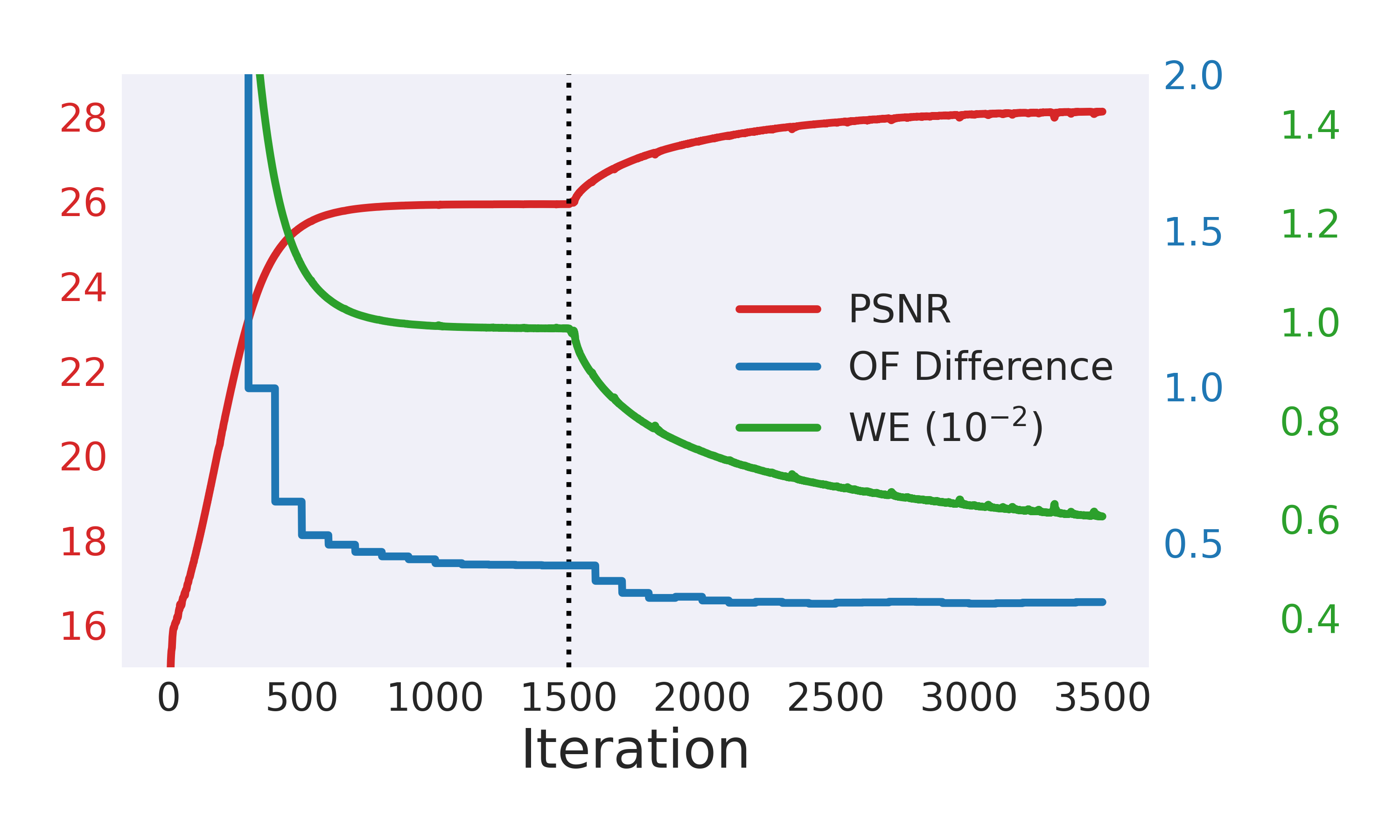
Figure 3: Evolution of key metrics during the iterative VR process: PSNR, OF difference (measured against ground truth), and warping error (WE). All metrics improve in early iterations. After OF difference stabilizes (vertical dotted line), progressive warping is activated, further enhancing PSNR and reducing WE, demonstrating our framework’s effectiveness for temporal consistency.

In practice, we introduce the warping loss $\mathcal{L}_{\text{warp}}$ only after the estimated frames $\mathbf{x}^{\prime}_{1},\dots,\mathbf{x}^{\prime}_{N}$ attain sufficient quality, as early iterations often yield noisy results. The evolution of performance over iterations is illustrated in Fig.˜3; it shows an evident performance boost in both data fidelity and temporal consistency after incorporating the proposed warping loss. To reduce computation, we update the OFs every $P$ iterations instead of each. We term our approach progressive warping because the estimated OFs themselves are progressively refined during iterations. However, these estimated OFs can exhibit slight fluctuations, which can hinder stable training. To address this, we apply an exponential moving average (EMA) to smooth out the OFs:

$$\mathbf{f}^{(t)}_{n\rightarrow n+1}=\beta\mathbf{f}^{(t-1)}_{n\rightarrow n+1}+(1-\beta)\mathbf{f}^{\prime(t)}_{n\rightarrow n+1},$$ (10)

where $\mathbf{f}^{(t)}_{n\rightarrow n+1}$ is the stabilized flow at iteration $t$, $\mathbf{f}^{\prime(t)}_{n\rightarrow n+1}$ is the newly estimated flow, and $\beta\in[0,1)$ is the weighted averaging coefficient. This smoothing mechanism not only stabilizes the training process, but also enhances the temporal consistency of the OFs.

3.3 Boosting computational and memory efficiency

Efficient diffusion sampling

DDPMs typically require dozens or hundreds of sampling steps, inducing significant computational and memory burdens for our approach in Eq.˜7. To address this challenge, we implement the DDIM sampler for the reverse process $\mathcal{R}$, which enables us to skip intermediate steps while preserving generation quality. Surprisingly, we find that $4$ reverse steps are sufficient for our method to outperform the SOTA, as shown in Tab.˜1. Adding more steps does not provide substantial benefits and can even slightly degrade the results, possibly due to numerical issues from vanishing gradients. Hence, we take $4$ as the default number of reverse steps. We also implement gradient checkpointing techniques to further reduce memory costs.

Table 1: Ablation study on performance vs. the number of reverse steps in diffusion process $\mathcal{R}$, performed on the DAVIS dataset for video super-resolution $\times 4$.

Steps	PSNR$\uparrow$	SSIM$\uparrow$	LPIPS$\downarrow$	WE($10^{-2}$)$\downarrow$
SOTA [15]	26.03	0.717	0.339	1.411
2	27.87	0.785	0.324	0.742
4	27.95	0.790	0.321	0.725
10	27.70	0.777	0.347	0.746

Efficient reformulation via mean value theorem (MVT)

There is a potential computational bottleneck in Eq.˜7: When performing backpropagation with respect to $\mathbf{R}$, the term $\mathcal{R}\pqty{\mathbf{z}_{shared}\mathbb{1}^{\intercal}+\mathbf{R}}$ requires $N$ separate forward passes through $\mathcal{R}$, expensive both in computation and in memory when $N$ is large. To address this, we assume that $\mathcal{R}:\mathbb{R}^{d}\rightarrow\mathbb{R}^{d}$ is continuously differentiable, with the operator norm (i.e., the largest singular value) of the Jacobian uniformly bounded by $L$. Then, for all $i$, $\norm{\mathcal{R}\pqty{\mathbf{z}_{shared}+\mathbf{r}_{i}}-{\mathcal{R}\pqty{\mathbf{z}_{shared}}}}\leq L\norm{\mathbf{r}_{i}}_{2}\leq L\sigma$ by the multivariate mean-value theorem [36]. So we consider

$$\min_{\mathbf{z}_{shared},\mathbf{R}}\;\ell\pqty{\mathbf{Y},\mathcal{A}\pqty{\mathcal{D}\pqty{{\mathcal{R}\pqty{\mathbf{z}_{shared}}+\mathbf{R}}}}},\\ \text{s.t.}\;\|\mathbf{r}_{i}\|_{2}\leq L\sigma,\quad\forall i\in\{1,\ldots,N\}.$$ (11)

Since $\mathbf{R}$ is now outside the RDP $\mathcal{R}$, backpropagation through $\mathcal{R}$ is only needed for $\mathbf{z}_{shared}$, reducing both memory and computation by a factor of $N$. To further reduce the cost due to backpropagation, we repeat the above idea by decomposing the pre-trained decoder $\mathcal{D}$ as $\mathcal{D}=\mathcal{D}_{1}\circ\mathcal{D}_{2}$ and putting the learnable residuals as input to $\mathcal{D}_{1}$, leading to our final formulation

$$\min_{\mathbf{z}_{shared},\mathbf{R}}\;\ell\pqty{\mathbf{Y},\mathcal{A}\pqty{\mathcal{D}_{1}\pqty{\mathcal{D}_{2}\circ\mathcal{R}\pqty{\mathbf{z}_{shared}}+\mathbf{R}}}},\\ \text{s.t.}\;\|\mathbf{r}_{i}\|_{2}\leq L^{\prime}\sigma,\quad\forall i\in\{1,\ldots,N\}.$$ (12)

Here, $L^{\prime}$ depends on both $L$ and also the maximum operator norm of the Jacobian of $\mathcal{D}_{2}$, and accounts for the maximum amplification of perturbations through $\mathcal{D}_{2}\circ\mathcal{R}$, ensuring rigorous bounds and applicability of our formulation to long video sequences. In practice, we place the trainable $\mathbf{R}$ directly on the last layer of $\mathcal{D}$. We set $L^{\prime}\sigma$ as $C\sqrt{\mathrm{dimension}(\mathbf{r}_{i})}$ for all $i$, where $C$ is a tunable hyperparameter.

Lightweight low-rank residual parameterization

For VR, the trainable residuals $\mathbf{r}_{1},\ldots,\mathbf{r}_{N}$ are high-dimensional tensors. In our implementation with Stable Diffusion, for example, the last layer of $\mathcal{D}$ has dimension $(1,128,512,512)$ for each residual. This leads to substantial memory and computation burdens. We address this by enforcing low-rank structures on the residuals. Specifically, we decompose each residual along its spatial dimensions as: $\mathbf{r}_{n}=\mathbf{A}_{n}\mathbf{B}_{n}$, where $\mathbf{A}_{n}\in\mathbb{R}^{1\times 128\times 512\times k}$ and $\mathbf{B}_{n}\in\mathbb{R}^{1\times 128\times k\times 512}$ with $k\ll 512$. This reduces the total parameter count for $\mathbf{R}$ from $O(N\cdot 128\cdot 512\cdot 512)$ to $O(N\cdot 128\cdot 512\cdot 2k)$, resulting in significant computational savings. To make the low-rank parameterization compatible with the PGD algorithm to solve Eq.˜12, we need to ensure $\norm{\mathbf{A}_{n}\mathbf{B}_{n}}\leq L^{\prime}\sigma$ for all $i$. For this, we take the heuristic projection

$$(\mathbf{A}_{n}^{\prime},\mathbf{B}_{n}^{\prime})\leftarrow(\mathbf{A}_{n},\mathbf{B}_{n})/\sqrt{\|\mathbf{A}_{n}\mathbf{B}_{n}\|/L^{\prime}\sigma},$$ (13)

after each gradient step on $(\mathbf{A}_{n},\mathbf{B}_{n})$. This produces a feasible $\mathbf{r}_{n}$, as $\norm{\mathbf{A}_{n}^{\prime}\mathbf{B}_{n}^{\prime}}=\norm{\mathbf{A}_{n}\mathbf{B}_{n}}/(\norm{\mathbf{A}_{n}\mathbf{B}_{n}}/L^{\prime}\sigma)=L^{\prime}\sigma$. With extra analytical and computational efforts, it is possible to develop a rigorous orthogonal projector here. But, we stick to this simple one, as it is easy to implement and effective in practice.

Algorithm 1 Our video restoration framework

1:Epochs $E$, transition $E_{T}$, diffusion steps $T$, $\mathbf{Y}$, $\mathcal{A}$

2:Initialize $\mathbf{z}_{shared}^{0}\sim\mathcal{N}\pqty{\mathbf{0},\mathbf{I}}$ and residuals $\mathbf{r}_{1}^{0},\cdots\mathbf{r}_{N}^{0}$

3:for $e=0$ to $E-1$ do

4:  for $i=T-1$ to $0$ do

5:   $\hat{\mathbf{s}}\leftarrow\mathbf{\varepsilon}_{\mathbf{\theta}}^{(i)}\pqty{\mathbf{z}_{i}^{e}}$

6:   $\hat{\mathbf{z}}_{0}^{e}\leftarrow\frac{1}{\sqrt{\bar{\alpha}_{i}}}\pqty{\mathbf{z}_{i}^{e}-\sqrt{1-\bar{\alpha}_{i}}\hat{\mathbf{s}}}$

7:   $\mathbf{z}_{i-1}^{e}\leftarrow$ DDIM reverse with $\hat{\mathbf{z}}_{0}^{e},\hat{\mathbf{s}}$

8:  end for

9:  ## Current reconstruction for $n-$th frame

10:  $\mathbf{x}^{\prime}_{n}=\mathcal{D}_{1}\pqty{\mathcal{D}_{2}\circ\mathcal{R}\pqty{\mathbf{z}_{shared}^{e}}+\mathbf{r}_{n}^{e}}$

11:  if $e>=E_{T}$ then

12:   $\mathbf{f}^{\prime(e)}_{n\rightarrow n+1}\leftarrow\text{stopgrad}\pqty{\textbf{RAFT}(\mathbf{x}^{\prime}_{n},\mathbf{x}^{\prime}_{n+1})}$

13:   $\mathbf{f}^{(e)}_{n\rightarrow n+1}=\beta\mathbf{f}^{(e-1)}_{n\rightarrow n+1}+(1-\beta)\mathbf{f}^{\prime(e)}_{n\rightarrow n+1}$

14:   Calculate $\mathcal{L}_{\text{warp}}$ via Sec.˜3.2.2

15:  else

16:   $\mathcal{L}_{\text{warp}}=0$

17:  end if

18:  Update $\mathbf{z}_{shared}^{e+1},\mathbf{r}_{1}^{e+1},\cdots,\mathbf{r}_{N}^{e+1}$ via Eq.˜12 with $\mathcal{L}_{\text{warp}}$

19:  Project each $\mathbf{r}_{n}^{e+1}$ onto $\ell_{2}$ norm ball

20:end for

21:Recovered video $\left[\mathbf{x}^{\prime}_{1},\dots,\mathbf{x}^{\prime}_{N}\right]$, where $\mathbf{x}^{\prime}_{n}=\mathcal{D}_{1}\pqty{\mathcal{D}_{2}\circ\mathcal{R}\pqty{\mathbf{z}_{shared}^{E}}+\mathbf{r}_{n}^{E}}$

4 Experiments

Experimental setup

We conduct comprehensive experiments on five VR tasks that involve various spatial and temporal degradations, following the protocols in [14, 15, 13]. The first three tasks involve spatial degradation only: (1) $4\times$ super-resolution, where low-resolution capture is simulated by applying $4\times$ average pooling to high-resolution videos; (2) inpainting with random masking at a missing rate of $r=0.5$; and (3) motion deblurring, where blurry videos are simulated by applying a $33\times 33$ motion blur kernel of strength $0.5$ to clean videos. In addition, we examine (4) temporal deconvolution, where degraded videos are generated by applying a uniform point-spread-function (PSF) convolution of width $7$ along the temporal dimension, simulating the common artifact that multiple frames blend together in time-varying video capturing. The last task (5) temporal deconvolution with spatial deblurring combines (4) temporal deconvolution and (3) spatial motion deblurring, representing complex real-world scenarios.

To generate evaluation datasets, we apply the above degradation models to four standard video benchmarks: DAVIS [37], REDS [9], SPMCS [38], and UDM10 [39]. To ensure consistent evaluation conditions, we process all videos by first segmenting them into sequential chunks of $8$ frames each, then center-cropping and resizing each frame to a uniform resolution of $512\times 512$ pixels.

We measure restoration quality using three standard spatial metrics: peak signal-to-noise ratio (PSNR), structural similarity index (SSIM), and learned perceptual image patch similarity (LPIPS, with the VGG backbone) [40]. To assess temporal consistency, we employ warping error (WE) [41], a metric widely adopted in video processing research [1, 13, 12, 5, 28]. For all experiments, we compute OFs using RAFT [35] and apply forward-backward consistency checking to generate non-occlusion masks for WE calculation.

Competing methods

While our work focuses on zero-shot methods for VR using pre-trained image DMs, we benchmark our proposed method against both zero-shot and supervised methods. To ensure fair comparison, we select methods with publicly available implementations and evaluate them using their default settings wherever possible. For zero-shot methods, we compare against SVI [14], VISION-XL (with SDXL) [15], VISION-base (with SD-base) [15], and DiffIR2VR (for super-resolution only) [12]. For supervised methods, our benchmarks include the following: SD $\times 4$ [25], VRT [4], RealBasicVSR [2], StableSR [3], and Upscale-A-Video (UAV) [1] for super-resolution; SD Inpainting [25] and ProPainter [5] for inpainting; and VRT [4], DeBlurGANv2 [42], Stripformer [43], and ID-Blau [44] for motion deblurring and/or temporal deconvolution. In all tables included in Sec.˜4.1, supervised and zero-shot methods are above and below the dotted line, respectively.

Implementations details

For all experiments except ablation studies, we use the pretrained Stable Diffusion (SD) 2.1-base model from [25]  and apply only $4$ reverse sampling steps ($T$) for $\mathcal{R}$ in our method. For text embeddings, we employ null-text following [45]. For the training objective, we employ a combination of MSE and perceptual loss [40] (with weight = $0.1$) as the loss function $\ell$ for both data fidelity (Eq.˜12) and progressive warping, except for inpainting tasks where we only use MSE for data fidelity. We set the learning rates as $5\text{\times}{10}^{-2}$ for the shared input seed $\mathbf{z}$ and $1\text{\times}{10}^{-3}$ for the residuals. We use ADAM [46] to solve the proposed formulation, which takes a total of $7$K iterations, with the progressive warping module activated after the initial $1.5$K iterations. To automate the activation of the progressive warping module, one could consider the quality of OF estimation and borrow ideas from zero-shot image restoration [47, 48]—a direction we leave for future work. The rank of the decomposed residual tensors is set to $k=32$, empirically a good balance between computational efficiency and expressiveness. We leave the implementation details of the competing methods in Appendix˜A.

4.1 Results

Table 2: (Spatial task) Quantitative comparisons for video super-resolution $\times 4$ (Bold: best, under: second best, green: performance increase, red: performance decrease)

Methods	DAVIS				REDS
	PSNR$\uparrow$	SSIM$\uparrow$	LPIPS$\downarrow$	WE($10^{-2}$)$\downarrow$	PSNR$\uparrow$	SSIM$\uparrow$	LPIPS$\downarrow$	WE($10^{-2}$)$\downarrow$
SD $\times 4$ [25]	24.33	0.615	0.358	1.523	23.57	0.619	0.371	1.769
VRT [4]	25.97	0.780	0.295	1.063	24.54	0.756	0.305	1.266
RealBasicVSR [2]	26.34	0.734	0.294	0.962	26.31	0.759	0.260	1.019
StableSR [3]	22.56	0.590	0.339	1.977	21.27	0.578	0.342	2.535
UAV [1]	23.65	0.589	0.397	1.623	23.02	0.593	0.422	1.920
DiffIR2VR [12]	25.01	0.637	0.337	1.321	24.14	0.633	0.328	1.592
SVI [14]	23.19	0.562	0.457	1.796	21.93	0.534	0.496	2.322
VISION-XL [15]	26.95	0.749	0.349	0.981	25.71	0.725	0.377	1.215
VISION-base [15]	26.17	0.712	0.338	1.137	24.95	0.687	0.376	1.406
Ours	28.21	0.799	0.315	0.698	27.40	0.792	0.339	0.824
Ours vs. Best compe.	+1.26	+0.019	+0.021	-0.264	+1.09	+0.033	+0.079	-0.195

Table 3: (Spatial task) Quantitative comparisons for video inpainting with random masking $50\%$ pixels (Bold: best, under: second best, green: performance increase, red: performance decrease)

Methods	DAVIS				REDS
	PSNR$\uparrow$	SSIM$\uparrow$	LPIPS$\downarrow$	WE($10^{-2}$)$\downarrow$	PSNR$\uparrow$	SSIM$\uparrow$	LPIPS$\downarrow$	WE($10^{-2}$)$\downarrow$
SD Inpainting [25]	16.98	0.258	0.679	6.776	15.77	0.238	0.677	9.253
ProPainter [5]	28.60	0.823	0.281	0.655	28.05	0.827	0.273	0.733
SVI [14]	25.80	0.699	0.318	1.134	24.61	0.679	0.323	1.389
VISION-XL [15]	29.93	0.862	0.186	0.612	28.66	0.840	0.207	0.745
VISION-base [15]	26.54	0.732	0.286	1.033	25.30	0.711	0.293	1.268
Ours	34.27	0.947	0.124	0.273	33.19	0.942	0.125	0.347
Ours vs. Best compe.	+4.34	+0.085	-0.062	-0.339	+4.53	+0.102	-0.082	-0.386

Table 4: (Spatial task) Quantitative comparisons for video motion debluring (Bold: best, under: second best, green: performance increase, red: performance decrease)

Methods	DAVIS				REDS
	PSNR$\uparrow$	SSIM$\uparrow$	LPIPS$\downarrow$	WE($10^{-2}$)$\downarrow$	PSNR$\uparrow$	SSIM$\uparrow$	LPIPS$\downarrow$	WE($10^{-2}$)$\downarrow$
VRT [4]	22.98	0.576	0.459	2.35	22.56	0.593	0.465	2.392
DeBlurGANv2 [42]	24.32	0.649	0.371	1.734	24.11	0.677	0.368	1.722
Stripformer [43]	24.07	0.612	0.381	2.218	24.72	0.699	0.343	1.797
ID-Blau [44]	23.07	0.589	0.397	2.623	23.84	0.654	0.359	2.198
SVI [14]	12.57	0.259	0.672	26.566	13.61	0.287	0.656	19.592
VISION-XL [15]	19.08	0.454	0.539	8.421	17.27	0.410	0.567	9.157
VISION-base [15]	12.81	0.290	0.699	26.359	13.98	0.320	0.684	21.882
Ours	31.70	0.889	0.211	0.443	30.33	0.873	0.250	0.543
Ours vs. Best compe.	+7.38	+0.240	-0.160	-1.291	+5.61	+0.174	-0.093	-1.179

Table 5: (Temporal task) Quantitative comparisons for video temporal deconvolution (Bold: best, under: second best, green: performance increase, red: performance decrease)

Methods	DAVIS				REDS
	PSNR$\uparrow$	SSIM$\uparrow$	LPIPS$\downarrow$	WE($10^{-2}$)$\downarrow$	PSNR$\uparrow$	SSIM$\uparrow$	LPIPS$\downarrow$	WE($10^{-2}$)$\downarrow$
VRT [4]	21.07	0.594	0.418	3.383	19.80	0.552	0.455	4.519
DeBlurGANv2 [42]	20.89	0.586	0.414	3.514	19.58	0.544	0.446	4.734
Stripformer [43]	20.75	0.565	0.411	3.638	19.49	0.524	0.453	4.893
ID-Blau [44]	18.42	0.491	0.476	6.128	17.73	0.467	0.515	6.968
SVI [14]	27.63	0.766	0.151	0.901	26.14	0.740	0.162	1.119
VISION-XL [15]	31.79	0.908	0.125	0.501	30.21	0.889	0.136	0.607
VISION-base [15]	27.66	0.767	0.151	0.897	26.17	0.741	0.162	1.115
Ours	32.965	0.948	0.104	0.317	33.307	0.952	0.099	0.362
Ours vs. Best compe.	+1.17	+0.040	-0.021	-0.184	+3.09	+0.063	-0.037	-0.245

Table 6: (Spatio-temporal task) Quantitative comparisons for video temporal deconvolution with spatial deblurring (Bold: best, under: second best, green: performance increase, red: performance decrease)

Methods	DAVIS				REDS
	PSNR$\uparrow$	SSIM$\uparrow$	LPIPS$\downarrow$	WE($10^{-2}$)$\downarrow$	PSNR$\uparrow$	SSIM$\uparrow$	LPIPS$\downarrow$	WE($10^{-2}$)$\downarrow$
VRT [4]	19.76	0.48	0.593	4.044	18.71	0.445	0.638	5.325
DeBlurGANv2 [42]	19.91	0.496	0.556	3.921	18.89	0.460	0.600	5.219
Stripformer [43]	20.00	0.503	0.548	3.879	18.88	0.458	0.588	5.224
ID-Blau [44]	19.76	0.489	0.554	4.060	18.73	0.450	0.593	5.418
SVI [14]	12.21	0.260	0.705	27.955	12.27	0.255	0.711	28.575
VISION-XL [15]	15.94	0.346	0.627	15.220	16.70	0.393	0.637	12.675
VISION-base [15]	12.17	0.262	0.727	30.325	11.92	0.269	0.732	30.436
Ours	26.97	0.778	0.343	0.852	26.61	0.763	0.381	0.982
Ours vs. Best compe.	+6.97	+0.275	-0.205	-3.027	+7.72	+0.303	-0.207	-4.237

As shown in Tabs.˜2, 3, 4, 5 and 6, our proposed method consistently outperforms existing ones across all VR tasks for almost all metrics on both the DAVIS and REDS datasets. We achieve consistent PSNR gains, ranging from 1–1.3dB in super-resolution, to the remarkable 6–8dB in combined degradation tasks, confirming our method’s effectiveness across levels of degradation complexity. Most notably, our method delivers substantial improvements in temporal consistency, with Warping Error (WE) reductions ranging from 0.18–0.26 in simpler tasks and dramatic 3–4.2 in combined temporal deconvolution with spatial deblurring. Similar performance trends are also observed in the SPMCS and UDM10 datasets, with detailed results provided in Appendix˜B. We also include qualitative comparisons in Appendix˜B.

In particular, here, the test distribution may differ from the original training distribution for both supervised and zero-shot methods, potentially explaining the noticeable performance degradation compared to their originally reported results. Although we include supervised methods just for reference given their very different setting compared to the zero-shot approach we focus on, their relatively poor performance highlights their limited generalizability when confronted with real-world distribution shifts. For zero-shot competitors, our method consistently outperforms them by large margins in both spatial metrics and, most significantly, temporal consistency. These results validate the effectiveness of our proposed formulation in Eq.˜12 and our hierarchical framework for bilevel temporal consistency described in Sec.˜3.2.

A particularly interesting observation is that CG-based methods [14, 15] perform uniformly poorly on motion deblur-related tasks, as is evident in Tabs.˜4 and 6. This observation is consistent with our theoretical analysis in Sec.˜2, which highlighted that CG requires the degradation operator $\mathcal{A}$ be known, symmetric and positive definite [31]. When CG deals with VR tasks that violate these mathematical requirements—such as motion deblurring—numerical issues arise, leading to poor performance. This limitation comprises a critical weakness in the SOTA CG-based methods, whereas our method is versatile and remains effective for different degradation scenarios.

4.2 Ablation studies

Effects of noise prior and progressive warping

Tab.˜7 presents the quantitative results of our ablation studies on the DAVIS dataset for video super-resolution. The integration of noise prior significantly improves the baseline model performance in terms of both PSNR and SSIM, while substantially reducing WE, signifying enhanced semantic-level temporal consistency. Progressive warping yields even stronger results with marked improvements in all metrics compared to the baseline, particularly in WE, indicating superior pixel-level temporal consistency. Notably, combining both components produces the optimal configuration, with our complete model outperforming an SOTA method [15] in all metrics. These results confirm that the noise prior and progressive warping mechanisms complement each other in promoting bilevel temporal consistency.

Effect of controllable residuals

We also study how the learning rate for residuals (LR_r) and the radius of residual balls (ie, controlling the magnitude of residuals) affect the performance. Intuitively, the residuals should not be too large to allow substantial deviation from the image manifold, and not be too small to limit their powers in modeling reasonable framewise deviation from the shared frame. This intuition is confirmed by our data in Tab.˜8: a restrictive radius (0.1) prevents adequate motion learning, whereas a moderate radius (1.0) allows effective discrepancy modeling; similarly, learning rate calibration is critical—a high rate (0.01) causes residual learning to dominate and downplays the influence from the DM prior, while an insufficient rate (0.0001) limits framewise adaptation. The optimal configuration (LR_r=0.001, radius=1.0) achieves the best performance by balancing these competing factors.

Table 7: Ablation study on two essential components for bilevel temporal consistency, performed on DAVIS dataset for video super-resolution $\times 4$. (Bold: best, under: second best)

Method	PSNR$\uparrow$	SSIM$\uparrow$	LPIPS$\downarrow$	WE($10^{-2}$)$\downarrow$
SOTA [15]	26.03	0.717	0.339	1.411
Base	24.70	0.612	0.366	1.398
Base with noise prior	26.09	0.703	0.410	1.057
Base with warping	27.14	0.736	0.301	0.943
Base with both	27.95	0.790	0.321	0.725

Table 8: Ablation study on the trainable residuals, performed on DAVIS dataset for video super-resolution $\times 4$.

LRr	Radius	PSNR$\uparrow$	SSIM$\uparrow$	LPIPS$\downarrow$	WE($10^{-2}$)$\downarrow$
0.01	0.1	24.36	0.654	0.436	1.557
	1.0	27.19	0.741	0.402	0.804
	10.0	27.16	0.739	0.405	0.806
0.001	0.1	25.74	0.719	0.374	1.161
	1.0	27.95	0.790	0.321	0.725
	10.0	27.91	0.789	0.324	0.737
0.0001	0.1	25.11	0.677	0.389	1.298
	1.0	26.17	0.709	0.366	1.096
	10.0	26.17	0.710	0.369	1.089

5 Discussion

In this paper, we focus on solving video restoration (VR) problems using pre-trained image DMs. We systematically address three key challenges: approximation errors through a novel MAP framework that reparameterizes frames directly in the seed space of LDMs; temporal inconsistency via a hierarchical bilevel consistency strategy; and high computational and memory demands through reformulation and low-rank decomposition. Comprehensive experiments show that our method significantly improves over state-of-the-art methods across various VR tasks without task-specific training, in terms of both frame quality and temporal consistency.

As for limitations, our empirical results in Tab.˜1 suggest a fundamental gap between image generation and regression using pretrained DMs, while Fig.˜2 shows the seed space clustering phenomenon we have not fully explained. Our work remains primarily empirical, and we leave a solid theoretical understanding for future research.

Appendix A More implementation details

Implementations of competing methods

We implement most competing methods using their default code and settings. For SVI, we adapt the implementation from the VISION-XL codebase by deactivating both the low-pass filter and DDIM inversion initialization. To ensure a fair comparison, we use the Stable Diffusion 2.1-base as the backbone for SVI. Similarly, for VISION-base, we modify the VISION-XL code and also take Stable Diffusion 2.1-base as the backbone. When applying SVI, VISION-XL, and VISION-base to motion-deblurring tasks, we implement an additional stopping mechanism that is activated just before the numerical issue due to conjugate gradient (CG) arises. This modification is necessary because, as discussed in Sec.˜2, CG requires the degradation operator $\mathcal{A}$ to be known, symmetric, positive definite to have guaranteed convergence and be free from numerical problems [31]. Motion deblurring operations inherently violate these CG requirements, as the degradation operators involved are asymmetric and tend to be ill-conditioned. The official implementations used for all competitors are listed below.

• SVI [14]: https://github.com/vision-xl/codes

• VISION-XL (with SDXL) [15]: https://github.com/vision-xl/codes

• VISION-base (with SD-base) [15]: https://github.com/vision-xl/codes

• DiffIR2VR [12]: https://github.com/jimmycv07/DiffIR2VR-Zero

• SD $\times 4$ [25]: https://github.com/Stability-AI/stablediffusion

• VRT [4]: https://github.com/JingyunLiang/VRT

• RealBasicVSR [2]: https://github.com/ckkelvinchan/RealBasicVSR

• StableSR [3]: https://github.com/IceClear/StableSR

• Upscale-A-Video (UAV) [1]: https://github.com/sczhou/Upscale-A-Video

• SD Inpainting [25]: https://github.com/Stability-AI/stablediffusion

• ProPainter [5]: https://github.com/sczhou/ProPainter

• DeBlurGANv2 [42]: https://github.com/VITA-Group/DeblurGANv2

• Stripformer [43]: https://github.com/pp00704831/Stripformer-ECCV-2022-

• ID-Blau [44]: https://github.com/plusgood-steven/ID-Blau

Appendix B More experiment results

B.1 Quantitative results

We provide more quantitative results for the five video restoration problems, including super-resolution, inpainting, motion deblurring, temporal deconvolution, and temporal deconvolution with spatial deblurring on SPMCS and UDM10 in Tabs.˜9, 10, 11, 12 and 13.

Table 9: (Spatial task) Quantitative comparisons for video super-resolution $\times 4$ (Bold: best, under: second best, green: performance increase, red: performance decrease)

Methods	SPMCS				UDM10
	PSNR$\uparrow$	SSIM$\uparrow$	LPIPS$\downarrow$	WE($10^{-2}$)$\downarrow$	PSNR$\uparrow$	SSIM$\uparrow$	LPIPS$\downarrow$	WE($10^{-2}$)$\downarrow$
SD $\times 4$ [25]	23.71	0.631	0.365	2.094	26.57	0.749	0.323	0.921
VRT [4]	26.19	0.811	0.243	1.169	28.11	0.865	0.179	0.609
RealBasicVSR [2]	25.77	0.746	0.288	1.363	28.27	0.845	0.245	0.640
StableSR [3]	21.82	0.598	0.352	2.908	23.11	0.72	0.319	1.76
UAV [1]	23.05	0.611	0.383	2.351	25.59	0.750	0.331	1.049
DiffIR2VR [12]	24.61	0.649	0.347	1.906	27.41	0.793	0.290	0.824
SVI [14]	22.58	0.581	0.426	2.469	23.80	0.644	0.440	1.596
VISION-XL [15]	26.43	0.758	0.314	1.310	29.22	0.847	0.268	0.616
VISION-base [15]	25.74	0.718	0.321	1.572	28.63	0.828	0.247	0.713
Ours	27.40	0.793	0.298	1.073	31.32	0.886	0.254	0.413
Ours vs. Best compe.	+0.97	-0.018	+0.055	-0.096	+2.10	+0.021	+0.075	-0.196

Table 10: (Spatial task) Quantitative comparisons for video inpainting with random masking $50\%$ pixels (Bold: best, under: second best, green: performance increase, red: performance decrease)

Methods	SPMCS				UDM10
	PSNR$\uparrow$	SSIM$\uparrow$	LPIPS$\downarrow$	WE($10^{-2}$)$\downarrow$	PSNR$\uparrow$	SSIM$\uparrow$	LPIPS$\downarrow$	WE($10^{-2}$)$\downarrow$
SD Inpainting [25]	16.62	0.276	0.709	8.969	15.28	0.243	0.758	10.533
ProPainter [5]	28.61	0.854	0.290	0.618	30.36	0.855	0.317	0.412
SVI [14]	25.92	0.746	0.334	1.360	28.05	0.817	0.323	0.658
VISION-XL [15]	30.14	0.894	0.178	0.527	32.04	0.906	0.199	0.345
VISION-base [15]	26.75	0.778	0.290	1.212	29.51	0.857	0.242	0.553
Ours	36.92	0.968	0.083	0.174	38.75	0.974	0.087	0.141
Ours vs. Best compe.	+6.78	+0.074	-0.095	-0.353	+6.71	+0.068	-0.112	-0.204

Table 11: (Spatial task) Quantitative comparisons for video motion debluring (Bold: best, under: second best, green: performance increase, red: performance decrease)

Methods	SPMCS				UDM10
	PSNR$\uparrow$	SSIM$\uparrow$	LPIPS$\downarrow$	WE($10^{-2}$)$\downarrow$	PSNR$\uparrow$	SSIM$\uparrow$	LPIPS$\downarrow$	WE($10^{-2}$)$\downarrow$
VRT [4]	22.85	0.572	0.431	3.133	23.38	0.694	0.39	2.315
DeBlurGANv2 [42]	24.47	0.674	0.338	2.181	25.40	0.776	0.299	1.465
Stripformer [43]	24.41	0.646	0.334	2.736	25.23	0.758	0.296	1.842
ID-Blau [44]	23.91	0.623	0.336	2.962	24.47	0.719	0.315	2.307
SVI [14]	14.12	0.310	0.645	24.896	14.66	0.369	0.677	20.061
VISION-XL [15]	18.89	0.452	0.514	12.202	19.87	0.559	0.495	5.560
VISION-base [15]	13.39	0.296	0.676	27.699	12.04	0.300	0.734	32.348
Ours	33.47	0.923	0.166	0.314	34.32	0.920	0.207	0.259
Ours vs. Best compe.	+9.00	+0.249	-0.168	-1.867	+8.92	+0.144	-0.089	-1.206

Table 12: (Temporal task) Quantitative comparisons for video temporal deconvolution (Bold: best, under: second best, green: performance increase, red: performance decrease)

Methods	SPMCS				UDM10
	PSNR$\uparrow$	SSIM$\uparrow$	LPIPS$\downarrow$	WE($10^{-2}$)$\downarrow$	PSNR$\uparrow$	SSIM$\uparrow$	LPIPS$\downarrow$	WE($10^{-2}$)$\downarrow$
VRT [4]	31.65	0.867	0.153	0.888	24.53	0.762	0.318	1.645
DeBlurGANv2 [42]	30.79	0.856	0.136	0.991	24.49	0.753	0.284	1.751
Stripformer [43]	31.38	0.861	0.121	0.969	24.81	0.757	0.247	1.798
ID-Blau [44]	29.37	0.838	0.140	1.290	24.38	0.753	0.256	1.973
SVI [14]	28.18	0.821	0.135	0.958	31.41	0.891	0.105	0.414
VISION-XL [15]	32.10	0.931	0.102	0.383	34.48	0.945	0.076	0.256
VISION-base [15]	28.21	0.821	0.135	0.954	31.44	0.891	0.104	0.412
Ours	40.45	0.987	0.030	0.095	36.67	0.971	0.079	0.180
Ours vs. Best compe.	+8.35	+0.056	-0.072	-0.288	+2.19	+0.026	+0.003	-0.076

Table 13: (Spatio-temporal task) Quantitative comparisons for video temporal deconvolution with spatial deblurring (Bold: best, under: second best, green: performance increase, red: performance decrease)

Methods	SPMCS				UDM10
	PSNR$\uparrow$	SSIM$\uparrow$	LPIPS$\downarrow$	WE($10^{-2}$)$\downarrow$	PSNR$\uparrow$	SSIM$\uparrow$	LPIPS$\downarrow$	WE($10^{-2}$)$\downarrow$
VRT [4]	22.14	0.548	0.488	3.343	22.15	0.661	0.472	2.594
DeBlurGANv2 [42]	23.32	0.638	0.383	2.498	22.83	0.685	0.426	2.257
Stripformer [43]	23.40	0.621	0.382	2.898	22.79	0.688	0.423	2.361
ID-Blau [44]	23.14	0.609	0.379	3.077	22.72	0.682	0.422	2.459
SVI [14]	12.70	0.273	0.670	29.942	13.66	0.363	0.693	23.061
VISION-XL [15]	18.39	0.460	0.535	10.862	17.68	0.500	0.5463	9.576
VISION-base [15]	12.84	0.291	0.694	28.502	12.40	0.334	0.742	33.661
Ours	30.87	0.886	0.215	0.535	29.88	0.857	0.292	0.534
Ours vs. Best compe.	+7.47	+0.248	-0.164	-1.963	+7.05	+0.169	-0.130	-1.723

B.2 Qualitative results

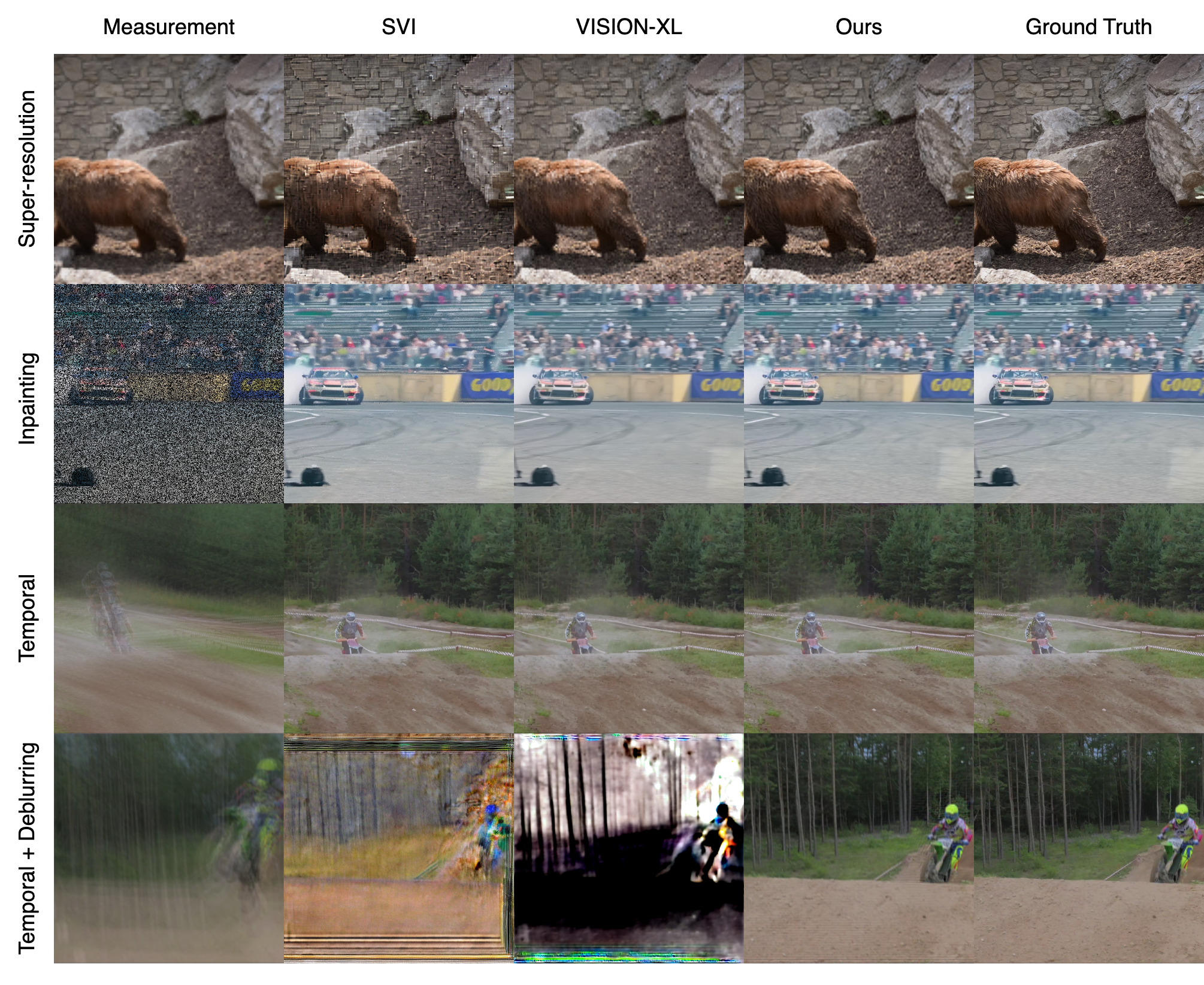
Figure 4: Qualitative comparisons on the DAVIS dataset: (a) Super-resolution $\times 4$, (b) Inpainting with $50\%$ random pixel masking, (c) Temporal deconvolution using uniform PSF with kernel width $k=7$, and (d) Temporal deconvolution with spatial deblurring.

We provide more qualitative results for the five video restoration problems, including super-resolution, inpainting, motion deblurring, temporal deconvolution, and temporal deconvolution with spatial deblurring on SPMCS and UDM10 in Figs.˜4, 5, 6, 7, 8 and 9.

Measurement

RealBasicVSR

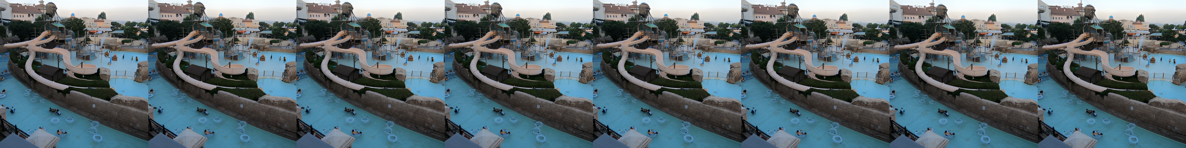
SVI

VISION-XL

Ours

Ground Truth

Figure 5: Qualitative comparisons for video super-resolution $\times 4$

Measurement

Pro Painter

SVI

VISION-XL

Ours

Ground Truth

Figure 6: Qualitative comparisons for video inpainting

Measurement

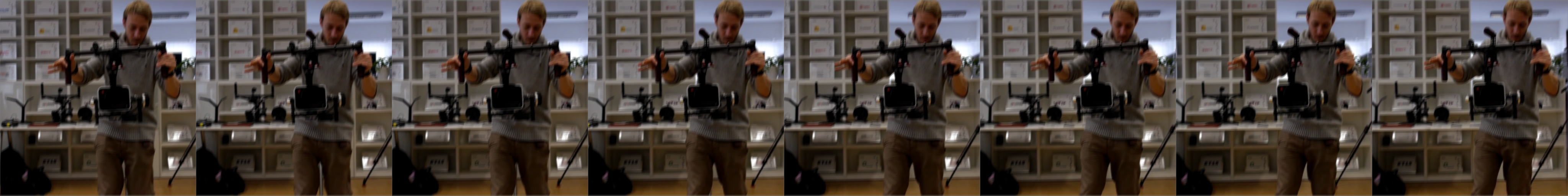
DeBlurGANv2

Stripformer

SVI

VISION-XL

Ours

Ground Truth

Figure 7: Qualitative comparisons for video motion deblurring

Measurement

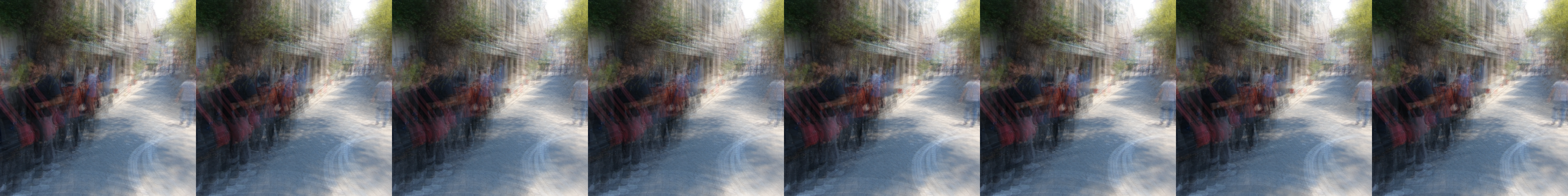
VRT

SVI

VISION-XL

Ours

Ground Truth

Figure 8: Qualitative comparisons for video temporal deconvolution

Measurement

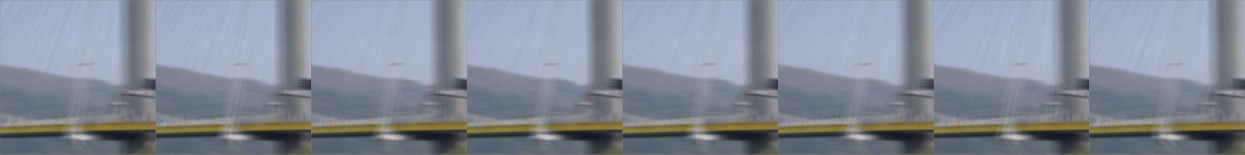
DeBlurGANv2

Stripformer

VISION-XL

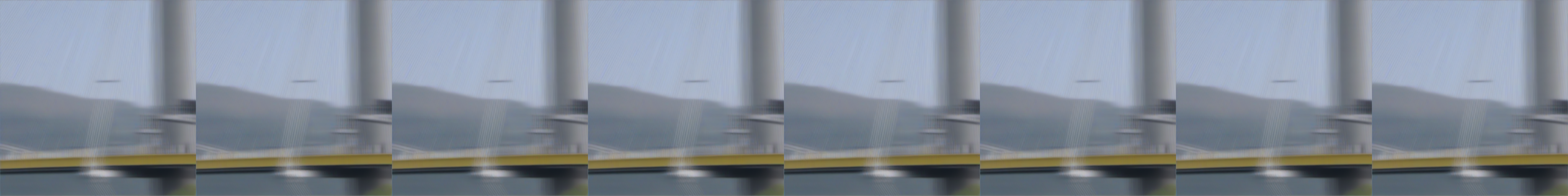
Ours

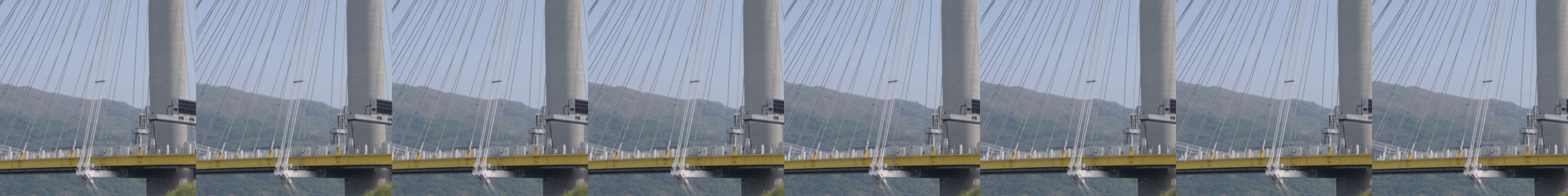
Ground Truth

Figure 9: Qualitative comparisons for video temporal deconvolution with spatial deblurring

References

- [1] S. Zhou, P. Yang, J. Wang, Y. Luo, and C. C. Loy, “Upscale-a-video: Temporal-consistent diffusion model for real-world video super-resolution,” in Proceedings of the IEEE/CVF Conference on Computer Vision and Pattern Recognition, 2024, pp. 2535–2545. [Online]. Available: https://openaccess.thecvf.com/content/CVPR2024/html/Zhou_Upscale-A-Video_Temporal-Consistent_Diffusion_Model_for_Real-World_Video_Super-Resolution_CVPR_2024_paper.html
- [2] K. C. K. Chan, S. Zhou, X. Xu, and C. C. Loy, “Investigating tradeoffs in real-world video super-resolution,” in Proceedings of the IEEE/CVF Conference on Computer Vision and Pattern Recognition, 2022, pp. 5962–5971. [Online]. Available: https://openaccess.thecvf.com/content/CVPR2022/html/Chan_Investigating_Tradeoffs_in_Real-World_Video_Super-Resolution_CVPR_2022_paper.html
- [3] J. Wang, Z. Yue, S. Zhou, K. C. K. Chan, and C. C. Loy, “Exploiting diffusion prior for real-world image super-resolution,” International Journal of Computer Vision, vol. 132, no. 12, pp. 5929–5949, 2024-12-01, company: Springer Distributor: Springer Institution: Springer Label: Springer Number: 12 Publisher: Springer US. [Online]. Available: https://link.springer.com/article/10.1007/s11263-024-02168-7
- [4] J. Liang, J. Cao, Y. Fan, K. Zhang, R. Ranjan, Y. Li, R. Timofte, and L. Van Gool, “VRT: A video restoration transformer,” IEEE Transactions on Image Processing, vol. 33, pp. 2171–2182, 2024. [Online]. Available: https://ieeexplore.ieee.org/document/10462902/
- [5] S. Zhou, C. Li, K. C. K. Chan, and C. C. Loy, “ProPainter: Improving propagation and transformer for video inpainting,” in Proceedings of the IEEE/CVF International Conference on Computer Vision, 2023, pp. 10 477–10 486. [Online]. Available: https://openaccess.thecvf.com/content/ICCV2023/html/Zhou_ProPainter_Improving_Propagation_and_Transformer_for_Video_Inpainting_ICCV_2023_paper.html
- [6] A. Lugmayr, M. Danelljan, A. Romero, F. Yu, R. Timofte, and L. Van Gool, “RePaint: Inpainting using denoising diffusion probabilistic models,” in Proceedings of the IEEE/CVF Conference on Computer Vision and Pattern Recognition, 2022, pp. 11 461–11 471. [Online]. Available: https://openaccess.thecvf.com/content/CVPR2022/html/Lugmayr_RePaint_Inpainting_Using_Denoising_Diffusion_Probabilistic_Models_CVPR_2022_paper.html
- [7] R. Xu, X. Li, B. Zhou, and C. C. Loy, “Deep flow-guided video inpainting,” in IEEE Conference on Computer Vision and Pattern Recognition, CVPR 2019, Long Beach, CA, USA, June 16-20, 2019. Computer Vision Foundation / IEEE, 2019, pp. 3723–3732. [Online]. Available: http://openaccess.thecvf.com/content_CVPR_2019/html/Xu_Deep_Flow-Guided_Video_Inpainting_CVPR_2019_paper.html
- [8] Z. Zhong, Y. Gao, Y. Zheng, and B. Zheng, “Efficient spatio-temporal recurrent neural network for video deblurring,” in Computer Vision – ECCV 2020. Springer, Cham, 2020, pp. 191–207, ISSN: 1611-3349. [Online]. Available: https://link.springer.com/chapter/10.1007/978-3-030-58539-6_12
- [9] S. Nah, S. Baik, S. Hong, G. Moon, S. Son, R. Timofte, and K. Mu Lee, “NTIRE 2019 Challenge on Video Deblurring and Super-Resolution: Dataset and Study,” pp. 0–0, 2019. [Online]. Available: https://openaccess.thecvf.com/content_CVPRW_2019/html/NTIRE/Nah_NTIRE_2019_Challenge_on_Video_Deblurring_and_Super-Resolution_Dataset_and_CVPRW_2019_paper.html
- [10] J. Ho, A. Jain, and P. Abbeel, “Denoising diffusion probabilistic models,” Advances in Neural Information Processing Systems, vol. 33, pp. 6840–6851, 2020. [Online]. Available: https://proceedings.neurips.cc/paper/2020/hash/4c5bcfec8584af0d967f1ab10179ca4b-Abstract.html
- [11] J. Song, C. Meng, and S. Ermon, “Denoising diffusion implicit models,” in International Conference on Learning Representations, 2020-10-02. [Online]. Available: https://openreview.net/forum?id=St1giarCHLP
- [12] C. Yeh, C.-Y. Lin, Z. Wang, C.-W. Hsiao, T.-H. Chen, H.-S. Shiu, and Y.-L. Liu, “DiffIR2vr-zero: Zero-shot video restoration with diffusion-based image restoration models.” [Online]. Available: https://openreview.net/forum?id=qpDqO7qa3R
- [13] C. Cao, H. Yue, X. Liu, and J. Yang, “Zero-shot Video Restoration and Enhancement Using Pre-Trained Image Diffusion Model,” arXiv.org, Jul. 2024. [Online]. Available: https://arxiv.org/abs/2407.01960v2
- [14] T. Kwon and J. C. Ye, “Solving video inverse problems using image diffusion models,” in The Thirteenth International Conference on Learning Representations, 2024-10-04. [Online]. Available: https://openreview.net/forum?id=TRWxFUzK9K
- [15] ——, “VISION-XL: High Definition Video Inverse Problem Solver using Latent Image Diffusion Models,” Nov. 2024. [Online]. Available: https://arxiv.org/abs/2412.00156v2
- [16] H. Chung, J. Kim, M. T. Mccann, M. L. Klasky, and J. C. Ye, “Diffusion posterior sampling for general noisy inverse problems,” in The Eleventh International Conference on Learning Representations, 2022-09-29. [Online]. Available: https://openreview.net/forum?id=OnD9zGAGT0k
- [17] D. Ulyanov, A. Vedaldi, and V. Lempitsky, “Deep image prior,” in Proceedings of the IEEE Conference on Computer Vision and Pattern Recognition, 2018, pp. 9446–9454. [Online]. Available: https://openaccess.thecvf.com/content_cvpr_2018/html/Ulyanov_Deep_Image_Prior_CVPR_2018_paper.html
- [18] X. Pan, X. Zhan, B. Dai, D. Lin, C. C. Loy, and P. Luo, “Exploiting deep generative prior for versatile image restoration and manipulation,” IEEE Transactions on Pattern Analysis and Machine Intelligence, vol. 44, no. 11, pp. 7474–7489, 2022-11, conference Name: IEEE Transactions on Pattern Analysis and Machine Intelligence. [Online]. Available: https://ieeexplore.ieee.org/abstract/document/9547753
- [19] Z. Zhuang, T. Li, H. Wang, and J. Sun, “Blind image deblurring with unknown kernel size and substantial noise,” International Journal of Computer Vision, vol. 132, no. 2, pp. 319–348, 2024-02-01, company: Springer Distributor: Springer Institution: Springer Label: Springer Number: 2 Publisher: Springer US. [Online]. Available: https://link.springer.com/article/10.1007/s11263-023-01883-x
- [20] T. Li, H. Wang, Z. Zhuang, and J. Sun, “Deep random projector: Accelerated deep image prior,” in IEEE/CVF Conference on Computer Vision and Pattern Recognition, CVPR 2023, Vancouver, BC, Canada, June 17-24, 2023. IEEE, 2023, pp. 18 176–18 185. [Online]. Available: https://doi.org/10.1109/CVPR52729.2023.01743
- [21] T. Li, Z. Zhuang, H. Wang, and J. Sun, “Random projector: Efficient deep image prior,” in IEEE International Conference on Acoustics, Speech and Signal Processing ICASSP 2023, Rhodes Island, Greece, June 4-10, 2023. IEEE, 2023, pp. 1–5. [Online]. Available: https://doi.org/10.1109/ICASSP49357.2023.10097088
- [22] H. Wang, X. Zhang, T. Li, Y. Wan, T. Chen, and J. Sun, “DMPlug: A plug-in method for solving inverse problems with diffusion models,” in The Thirty-eighth Annual Conference on Neural Information Processing Systems, 2024. [Online]. Available: https://openreview.net/forum?id=81IFFsfQUj
- [23] A. Hyvärinen, “Estimation of Non-Normalized Statistical Models by Score Matching,” Journal of Machine Learning Research, vol. 6, no. 24, pp. 695–709, 2005. [Online]. Available: http://jmlr.org/papers/v6/hyvarinen05a.html
- [24] Y. Song and S. Ermon, “Generative modeling by estimating gradients of the data distribution,” Advances in Neural Information Processing Systems, vol. 32, 2019. [Online]. Available: https://proceedings.neurips.cc/paper/2019/hash/3001ef257407d5a371a96dcd947c7d93-Abstract.html?ref=https://githubhelp.com
- [25] R. Rombach, A. Blattmann, D. Lorenz, P. Esser, and B. Ommer, “High-resolution image synthesis with latent diffusion models,” in Proceedings of the IEEE/CVF Conference on Computer Vision and Pattern Recognition, 2022, pp. 10 684–10 695. [Online]. Available: https://openaccess.thecvf.com/content/CVPR2022/html/Rombach_High-Resolution_Image_Synthesis_With_Latent_Diffusion_Models_CVPR_2022_paper
- [26] D. Podell, Z. English, K. Lacey, A. Blattmann, T. Dockhorn, J. Müller, J. Penna, and R. Rombach, “SDXL: Improving latent diffusion models for high-resolution image synthesis,” in The Twelfth International Conference on Learning Representations, 2023-10-13. [Online]. Available: https://openreview.net/forum?id=di52zR8xgf
- [27] W. Peebles and S. Xie, “Scalable diffusion models with transformers,” in Proceedings of the IEEE/CVF International Conference on Computer Vision, 2023, pp. 4195–4205. [Online]. Available: https://openaccess.thecvf.com/content/ICCV2023/html/Peebles_Scalable_Diffusion_Models_with_Transformers_ICCV_2023_paper.html
- [28] G. Daras, W. Nie, K. Kreis, A. Dimakis, M. Mardani, N. B. Kovachki, and A. Vahdat, “Warped diffusion: Solving video inverse problems with image diffusion models,” in The Thirty-eighth Annual Conference on Neural Information Processing Systems, 2024. [Online]. Available: https://openreview.net/forum?id=LH94zPv8cu
- [29] B. Fei, Z. Lyu, L. Pan, J. Zhang, W. Yang, T. Luo, B. Zhang, and B. Dai, “Generative diffusion prior for unified image restoration and enhancement,” in Proceedings of the IEEE/CVF Conference on Computer Vision and Pattern Recognition, 2023, pp. 9935–9946. [Online]. Available: https://openaccess.thecvf.com/content/CVPR2023/html/Fei_Generative_Diffusion_Prior_for_Unified_Image_Restoration_and_Enhancement_CVPR_2023_paper.html
- [30] H. Chung, S. Lee, and J. C. Ye, “Decomposed diffusion sampler for accelerating large-scale inverse problems,” in The Twelfth International Conference on Learning Representations, 2023-10-13. [Online]. Available: https://openreview.net/forum?id=DsEhqQtfAG
- [31] J. Shewchuk, “An Introduction to the Conjugate Gradient Method Without the Agonizing Pain,” Mar. 1994. [Online]. Available: https://www.semanticscholar.org/paper/An-Introduction-to-the-Conjugate-Gradient-Method-Shewchuk/70000f7791ab8519429ce939bc897738a05939c3
- [32] L. v. d. Maaten and G. Hinton, “Visualizing Data using t-SNE,” Journal of Machine Learning Research, vol. 9, no. 86, pp. 2579–2605, 2008. [Online]. Available: http://jmlr.org/papers/v9/vandermaaten08a.html
- [33] D. Sun, X. Yang, M.-Y. Liu, and J. Kautz, “PWC-net: CNNs for optical flow using pyramid, warping, and cost volume,” in Proceedings of the IEEE Conference on Computer Vision and Pattern Recognition, 2018, pp. 8934–8943. [Online]. Available: https://openaccess.thecvf.com/content_cvpr_2018/html/Sun_PWC-Net_CNNs_for_CVPR_2018_paper.html
- [34] S. Meister, J. Hur, and S. Roth, “UnFlow: Unsupervised learning of optical flow with a bidirectional census loss,” in Proceedings of the AAAI Conference on Artificial Intelligence, vol. 32, no. 1, 2018-04-27, number: 1. [Online]. Available: https://ojs.aaai.org/index.php/AAAI/article/view/12276
- [35] Z. Teed and J. Deng, “RAFT: Recurrent all-pairs field transforms for optical flow,” in Computer Vision – ECCV 2020. Springer, Cham, 2020, pp. 402–419, ISSN: 1611-3349. [Online]. Available: https://link.springer.com/chapter/10.1007/978-3-030-58536-5_24
- [36] R. Coleman, Calculus on normed vector spaces. Springer Science & Business Media, 2012.
- [37] F. Perazzi, J. Pont-Tuset, B. McWilliams, L. Van Gool, M. Gross, and A. Sorkine-Hornung, “A benchmark dataset and evaluation methodology for video object segmentation,” in 2016 IEEE Conference on Computer Vision and Pattern Recognition (CVPR). IEEE, 2016-06, pp. 724–732. [Online]. Available: https://ieeexplore.ieee.org/document/7780454/
- [38] X. Tao, H. Gao, R. Liao, J. Wang, and J. Jia, “Detail-revealing deep video super-resolution,” in Proceedings of the IEEE International Conference on Computer Vision, 2017, pp. 4472–4480. [Online]. Available: https://openaccess.thecvf.com/content_iccv_2017/html/Tao_Detail-Revealing_Deep_Video_ICCV_2017_paper.html
- [39] P. Yi, Z. Wang, K. Jiang, J. Jiang, and J. Ma, “Progressive Fusion Video Super-Resolution Network via Exploiting Non-Local Spatio-Temporal Correlations,” in 2019 IEEE/CVF International Conference on Computer Vision (ICCV), Oct. 2019, pp. 3106–3115, iSSN: 2380-7504. [Online]. Available: https://ieeexplore.ieee.org/document/9009484
- [40] R. Zhang, P. Isola, A. A. Efros, E. Shechtman, and O. Wang, “The unreasonable effectiveness of deep features as a perceptual metric,” in Proceedings of the IEEE Conference on Computer Vision and Pattern Recognition, 2018, pp. 586–595. [Online]. Available: https://openaccess.thecvf.com/content_cvpr_2018/html/Zhang_The_Unreasonable_Effectiveness_CVPR_2018_paper.html
- [41] W.-S. Lai, J.-B. Huang, O. Wang, E. Shechtman, E. Yumer, and M.-H. Yang, “Learning blind video temporal consistency,” in Proceedings of the European Conference on Computer Vision (ECCV), 2018, pp. 170–185. [Online]. Available: https://openaccess.thecvf.com/content_ECCV_2018/html/Wei-Sheng_Lai_Real-Time_Blind_Video_ECCV_2018_paper.html
- [42] O. Kupyn, T. Martyniuk, J. Wu, and Z. Wang, “DeblurGAN-v2: Deblurring (orders-of-magnitude) faster and better,” in Proceedings of the IEEE/CVF International Conference on Computer Vision, 2019, pp. 8878–8887. [Online]. Available: https://openaccess.thecvf.com/content_ICCV_2019/html/Kupyn_DeblurGAN-v2_Deblurring_Orders-of-Magnitude_Faster_and_Better_ICCV_2019_paper.html
- [43] F.-J. Tsai, Y.-T. Peng, Y.-Y. Lin, C.-C. Tsai, and C.-W. Lin, “Stripformer: Strip transformer for fast image deblurring,” in Computer Vision – ECCV 2022. Springer, Cham, 2022, pp. 146–162, ISSN: 1611-3349. [Online]. Available: https://link.springer.com/chapter/10.1007/978-3-031-19800-7_9
- [44] J.-H. Wu, F.-J. Tsai, Y.-T. Peng, C.-C. Tsai, C.-W. Lin, and Y.-Y. Lin, “Id-blau: Image deblurring by implicit diffusion-based reblurring augmentation,” in Proceedings of the IEEE/CVF Conference on Computer Vision and Pattern Recognition (CVPR), June 2024, pp. 25 847–25 856.
- [45] L. Rout, N. Raoof, G. Daras, C. Caramanis, A. Dimakis, and S. Shakkottai, “Solving linear inverse problems provably via posterior sampling with latent diffusion models,” in Thirty-seventh Conference on Neural Information Processing Systems, 2023-11-02. [Online]. Available: https://openreview.net/forum?id=XKBFdYwfRo
- [46] D. P. Kingma and J. Ba, “Adam: A method for stochastic optimization,” in 3rd International Conference on Learning Representations, ICLR 2015, San Diego, CA, USA, May 7-9, 2015, Conference Track Proceedings, Y. Bengio and Y. LeCun, Eds., 2015. [Online]. Available: http://arxiv.org/abs/1412.6980
- [47] T. Li, Z. Zhuang, H. Liang, L. Peng, H. Wang, and J. Sun, “Self-validation: Early stopping for single-instance deep generative priors,” in 32nd British Machine Vision Conference 2021, BMVC 2021, Online, November 22-25, 2021. BMVA Press, 2021, p. 108. [Online]. Available: https://www.bmvc2021-virtualconference.com/assets/papers/1633.pdf
- [48] H. Wang, T. Li, Z. Zhuang, T. Chen, H. Liang, and J. Sun, “Early stopping for deep image prior,” Transactions on Machine Learning Research, 2023. [Online]. Available: https://openreview.net/forum?id=231ZzrLC8X