Long-Moody construction of braid group representations and Haraoka’s multiplicative middle convolution for KZ-type equations

Abstract

In this paper, we establish a correspondence between algebraic and analytic approaches to constructing representations of the braid group $B_{n}$, namely Katz-Long-Moody construction and multiplicative middle convolution for Knizhnik-Zamolodchikov (KZ)-type equations, respectively. By the left action of the braid group $B_{n}$ on the free group $F_{n}$, known as the Artin representation, the semidirect product can be defined $F_{n}\rtimes B_{n}$. The Long-Moody construction [27] provides a method to construct linear representations of $B_{n}$ from any given representation of $F_{n}\rtimes B_{n}$. The Katz-Long-Moody construction generalizes this approach, yielding an infinite sequence of representations of $F_{n}\rtimes B_{n}$ [17]. On the other hand, the fundamental group of the domain of the $n$-valued KZ-type equation is isomorphic to the pure braid group $P_{n}$. The multiplicative middle convolution for the KZ-type equation provides an antirepresentation of $P_{n}$, derived from a given antirepresentation of $P_{n}$ [16]. Furthermore, we show that this construction preserves unitarity relative to a Hermitian matrix $\widetilde{H}_{\widetilde{p},\widetilde{q}}$, and established an algorithm to determine the signature of the Hermitian matrix $\widetilde{H}_{\widetilde{p},\widetilde{q}}$.

Keywords KZ-type equation  $\cdot$ representation of braid groups  $\cdot$ Long-Moody construction

1 Introduction

In 1994, Long introduced a method for constructing braid group representations by combining a generalization of the Magnus construction with an iterative process [27]. This approach connects braid groups to the automorphism group of free groups ($\text{Aut}(F_{n})$) and offers a geometric perspective that simplifies the analysis of faithfulness while enabling the systematic generation of new representations. Consider the Artin representation, $\theta:B_{n}\longrightarrow\operatorname{Aut}(F_{n})$, induced by left action of braid group $B_{n}$ on $\pi_{1}(D_{2}/\{n\text{-points}\})=F_{n}$. Then, we can define the semidirect product $F_{n}\rtimes_{\theta}B_{n}$. Long-Moody construction is the method to construct a representation of $B_{n}$, $\rho^{LM}\colon B_{n}\longrightarrow GL(V^{\oplus n})$, from any representation of $F_{n}\rtimes_{\theta}B_{n}$, $\rho\colon F_{n}\rtimes_{\theta}B_{n}\longrightarrow GL(V)$. The Long-Moody construction is a significant research subject from the perspectives of representation theory, the theory of linear differential equations in complex domains, and knot theory.

First, from the viewpoint of representation theory, the Long-Moody construction generalizes the Burau representation [7] derived from the Alexander polynomial of knots. Subsequent research has revealed that this construction yields important representations of braid groups [4], notably unitary representations. Consequently, the Long-Moody construction serves as a unifying framework for classifying various representations of braid groups. An open problem of particular interest is whether every unitary representation of a braid group can be obtained via the construction [6]. Furthermore, Soulié [31, 32] has extended the construction by generalizing the braid group actions from Artin representations to Wada representations [37, 18]. Braid group representations can also be derived through the generalization of Tong-Yang-Ma representations [35], aside from the Long-Moody construction.

Second, we discuss the viewpoint of linear differential equations in complex domains. The action of elements of the fundamental group of the domain on the solution space of a differential equation is known as the monodromy representation. An important example of differential equations whose fundamental group of the domain is a (pure) braid group is given by the $n$-variable Knizhnik-Zamolodchikov (KZ-type) equations. A significant study by Drinfeld, Kanie, Kohno, and Tsuchiya establishes the connection between monodromy representations of KZ equations and representations of braid groups [13, 36, 23]. It is also known that the Lawrence-Krammer-Bigelow representations [26] obtained by the construction relate to the monodromy representations of KZ equations.

Third, we discuss the viewpoint of knot theory. Since any link can be expressed as the closure of a braid [20], the study of braid groups contributes substantially to knot invariants. In particular, the Burau representation extends the Alexander polynomial, and it is known that twisted Alexander polynomials of knots can be obtained through the construction [34].

In our previous paper[17], we generalized the Long-Moody construction and obtained infinite sequences of braid group representations via the Katz-Long-Moody construction. The Katz-Long-Moody construction, by unifying Long-Moody construction and the twisted homology theory, the algorithm for constructing local systems on $\mathbb{C}/\{n\text{-points}\}$ introduced by Katz [21]. Katz’s foundational theory on rigid local systems extended by Dettweiler and Reiter[11]. They developed a method for reconstructing Fuchsian-type linear differential equations with finite singularities. Haraoka further extended this and constructed the method for reconstructing $n$ variable KZ-type equations[15, 16]. The KZ equation initially developed in conformal field theory as a differential equation for $n$-point correlation functions and has emerged as a central object of study. Solutions to the KZ equation, including Selberg-type integrals, are closely related to various special functions such as Appell-Lauricella hypergeometric series. KZ-type equation is a generalization of KZ equation.

In this paper, we establish a correspondence between the algebraic method of the Katz-Long-Moody construction and the analytic method of the middle convolution for KZ-type equations. In section 2, we provide an explicit formulation of the Katz-Long-Moody construction using matrix representations. In section 3, we interpret Dettweiler-Reiter’s method and Haraoka’s method as approaches to constructing representations of the free group $F_{n}$ and the pure braid group $P_{n}$, respectively. In section 3, we define a natural transformation that connects these methods.

The main theorem is the following. For a group homomorphism $\rho\colon P_{n+1}\longrightarrow\mathrm{GL}(V)$, let $\rho_{\lambda}^{\mathrm{LM}}$ be a generalized LM of $\rho$ for the generator $(\sigma_{ij})$ of $P_{n+1}$, and let $(\rho^{op})_{\lambda}^{\mathrm{H}}$ be a Haraoka convolution of $\rho^{op}$ for the generator $(\widetilde{\sigma_{ij}})$ of $P_{n+1}$. Let $\operatorname{op}$ be an antihomomorphism such that $\operatorname{op}\colon P_{n+1}\ni\sigma_{ij}\mapsto\widetilde{\sigma_{ij}}\in P_{n+1}$. Then we have

$$(\rho_{\lambda}^{\mathrm{LM}})^{op}=(\rho^{op})_{\lambda}^{\mathrm{H}}.$$

Using this natural transformation, the Haraoka-Long natural transformation, we propose an algorithm for computing how monodromy matrices change in response to basis transformations in the context of the multiplicative middle convolution. The natural transformation facilitates the mutual application of analytical and algebraic insights. One such example is the following result.

The second main theorem is about the unitarity of the representation. In this paper, we define unitarity differently from the definition given in the previous work [27], as follows:

Definition 1.1 (Unitarity of representation [27]).

Let $\rho\colon G\longrightarrow GL(V)$ be unitary relative to $H$ if there exists a non-degenerate Hermitian matrix $H$ such that $\rho(g)^{{\dagger}}H\rho(g)=H\text{ holds for any }g\in G.$

In [27], Long proved that if $\rho$ is unitary, so is $\rho^{LM}_{s}$ for some generic value $s$, according the method by Delingne-Mostow[9]. Here, $\rho^{LM,s}(\sigma_{i}):=s\cdot\rho^{LM}(\sigma_{i})$. We extend the result and show that unitarity is preserved by Katz-Long-Moody construction under some conditions. First, we construct a Hermitian matrix, not necessarily nondegenerate, that satisfies the unitarity condition. Finally, we show the algorithm to calculate the condition under which this Hermitian matrix becomes nondegenerate.

While the previous work required nondegenerate Hermitian matrix, our definition does not impose the nondegenerate to handle a more general context. Adopting this definition enables a more unified treatment of infinite sequence of monodromy invariant Hermitian matrix. A monodromy-invariant Hermitian form had already been obtained through the discussion of the KZ-type equation [14], and it was shown that this Hermitian matrix satisfies unitarity via Haraoka-Long natural transformation. This study demonstrated that the Katz-Long-Moody construction preserves unitarity relative to a Hermitian matrix. We showed that if $\rho$ is unitary relative to a Hermitian matrix $H_{p,q}$, we can construct a Hermitian matrix $\tilde{H}_{\widetilde{p},\widetilde{q}}$ by $H_{p,q}$. Furthermore, we established a recursive algorithm to determine the signature of the Hermitian matrix $\widetilde{H}_{\widetilde{p},\widetilde{q}}$. Previous study [12, 1] have examined the effects of middle convolution in the context of unitary rank-$1$ or rank-$2$ local systems, respectively. This research generalizes their results to unitary local systems of general rank-$N$ and proposed the algorithm to calculate the signature of the Hermitian form.

2 Algebraic construction of representation of braid group

2.1 Braid group

There are several ways to define the braid group $B_{n}$. To construct the bridge between the algebraic construction and the analytical construction of the braid group representations, it is necessary to consider both the algebraic definition and the topological definition.

Definition 2.1 (Artin’s braid group $B_{n}$ [2]).

The Artin braid group $B_{n}$ is the group generated by $n-1$ generators $\sigma_{1},\cdots,\sigma_{n-1}$ and two braid relations.

1. $\sigma_{i}\sigma_{j}=\sigma_{j}\sigma_{i}\ \ \ \ \ \ \ \ \ \ \ \ \ \ \ \ \ \phantom{|}(|j-i|>1)$

2. $\sigma_{i}\sigma_{i+1}\sigma_{i}=\sigma_{i+1}\sigma_{i}\sigma_{i+1}\ \ (i=1,\cdots,n-2).$

The braid group can also be defined as the mapping class group of a the $n$-punctured disc $D_{n}=D_{2}\setminus\{n-\text{points}\}$, $\operatorname{MCG}(D_{n},\partial D_{n})$ [5]. The generators of this group are half-twists $\tau_{i},i=1,\dots,n-1$, which are self-homeomorphisms that perform a $\pi$ rotation of an open disk containing only two adjacent points $a_{i}$ and $a_{i+1}$. A half-twist $\tau_{i}$ corresponds to the generator $\sigma_{i}$ of $B_{n}$.

Definition 2.2 (half-twist).

The generators of the mapping class group $\operatorname{MCG}(D,\partial D)$ of a closed disk with $n$ marked points include elements called half-twists.

Formally, let $a_{i},a_{i+1}$ be two distinct marked points in the interior of $D_{2}$. The half-twist associated with $a_{i}$ and $a_{j}$, denoted by $\tau_{i}$, is the isotopy class of a homeomorphism that:

1.

Exchanges $a_{i}$ and $a_{i+1}$,

2.

Twists the local neighborhood of the line segment connecting $a_{i}$ and $a_{i+1}$ by a half-turn in a counterclockwise direction,

3.

Fixes all other points and the boundary $\partial D$.

The braid group $B_{n}$ is naturally identified with the mapping class group $MCG(D_{n},\partial D_{n})$. The Artin representation is a homomorphism $\theta:B_{n}\to\operatorname{Aut}(F_{n})$ induced by the left action of $B_{n}$ on the fundamental group $\pi_{1}(D_{n})=F_{n}$, corresponding to half-twists. By defining this action of the braid group on the free group, we define $F_{n}\rtimes_{\theta}B_{n}$. There are various ways in the choice of the Artin representation, but the following definition is adopted for the purpose of defining the Katz-Long-Moody construction. Throughout the paper, we always consider left actions, hence we adapt the convention that $\operatorname{Aut}(F_{n})$ acts on $F_{n}$ from left.

Definition 2.3 (Artin representation).

Let $x_{1},\ldots,x_{n}$ be the generators of $F_{n}$. Define braid left action $\theta$ on $F_{n}$ as follows.

$$\begin{array}[]{cccc}\theta\colon&B_{n}&\stackrel{{\scriptstyle f}}{{\longrightarrow}}&\operatorname{Aut}(F_{n})\\ &\rotatebox{90.0}{$\in$}&&\rotatebox{90.0}{$\in$}\\ &\sigma_{i}&\longmapsto&\theta_{\sigma_{i}}\end{array}$$

$$\theta_{\sigma_{i}}(x_{j}):=\left\{\begin{array}[]{ll}x_{i+1}&j=i\\ x_{i+1}^{-1}x_{i}x_{i+1}&j=i+1\\ x_{j}&j\neq i,i+1\\ \end{array}\right..$$

Definition 2.4 (Semidirect product $F_{n}\rtimes_{\theta}B_{n}$).

The (outer) semidirect product of $B_{n}$ and $F_{n}$ with respect to $\theta$ is the group denoted by $F_{n}\rtimes_{\theta}B_{n}$, defined as follows:

1.

The underlying set of $F_{n}\rtimes_{\theta}B_{n}$ is the Cartesian product $F_{n}\times B_{n}$.

2.

The product is given by:

$$(h_{1},g_{1})\cdot(h_{2},g_{2})=(h_{1}\cdot\theta_{g_{1}}(h_{2}),g_{1}\cdot g_{2}),$$

where $h_{1},h_{2}\in F_{n}$, $g_{1},g_{2}\in B_{n}$, and $\theta_{g_{1}}(h_{2})$ denotes the action of $g_{1}$ on $h_{2}$ via $\theta$.

Here, we consider a geometric realization of the Artin representation as follows. First, we examine the space obtained by removing $n$ points from the interior of a closed disk. The fundamental group of this space is isomorphic to a free group. Selecting a point $d$ on the boundary of the disk as the base point, we consider $n$ loops, each starting at $d$, encircling one of the removed points counterclockwise exactly once, and returning to $d$. Labeling these loops as $x_{1},\dots,x_{n}$, they serve as the generators of the fundamental group. Hereinafter, we abbreviate the notation $\rtimes_{\theta}$ as simply $\rtimes$.

2.2 Settings for the algebraic construction

Notably, in [16], the author defined the path of analytic continuation following the convention of Katz’s theory. When considering the correspondence with the twisted Long-Moody construction, the geometric framework for defining the path plays a crucial role. Although the algebraic representation of the generators of the braid group remains the same, the definition of the half-twist, which serves as a generator of the mapping class group, admits two possible conventions. Specifically, it depends on whether $\sigma_{i}$ denotes a clockwise or counterclockwise rotation. Here, we adopt the convention that a counterclockwise rotation corresponds to the generator $\sigma_{i}$ of the braid group. Then, the generators $x_{i}$ of $F_{n}$ and the geometric realization of the Artin representation are defined in a manner consistent with this definition of the generators of $B_{n}$. The generator $x_{i}$ of the free group is represented as paths that loop clockwise around the point $x_{i}$.

• generators of $B_{n}$ : anticlockwise

• generators of $F_{n}$ : clockwise

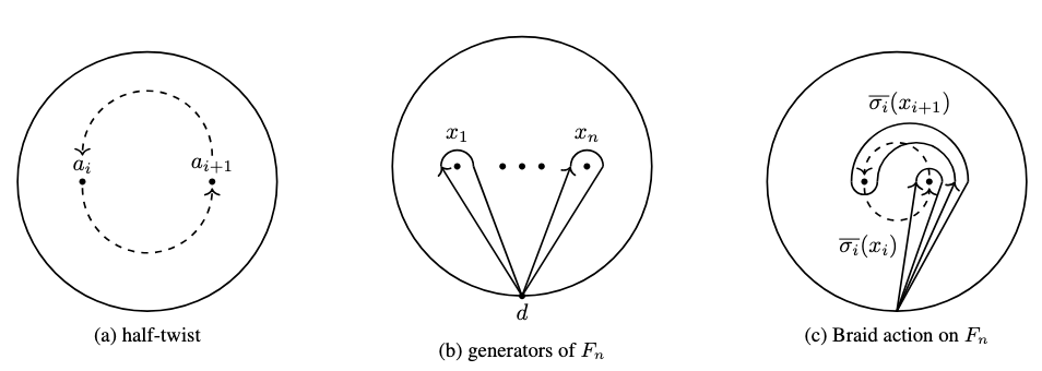
Figure 1: Geometric realization of Artin representation

The Artin representation corresponds to how the generators of the free group change when an element $\sigma_{i}$ of the braid group is given. When the action of the braid group is defined by a half-twist, the elements of the free group transform in accordance with the Artin representation. Hereafter, we denote the field by $\bm{k}$.

2.3 the Long-Moody construction

Definition 2.5 (Long-Moody construction).

Let $V$ be a finite dimensional $\bm{k}$-vector space.
For a group homomorphism $\rho$ with a generator of $F_{n}\rtimes B_{n},x_{j},\sigma_{i},(j=1,\dots,n,i=1,\dots,n-1)$,

$$\rho\colon F_{n}\rtimes B_{n}\longrightarrow\mathrm{GL}(V)$$

is given, then we have a following group homomorphism

$$\rho^{\mathrm{LM}}\colon B_{n}\longrightarrow\mathrm{GL}(V^{\oplus n})$$

where we denote

$$g_{i}:=\rho(x_{i}),\ s_{i}:=\rho(\sigma_{i}),$$

$$\rho^{\mathrm{LM}}(\sigma_{i}):=s_{i}^{\oplus n}\cdot\left(\begin{array}[]{ccc}I_{N(i-1)}&&\\ &R_{i}&\\ &&I_{N(n-i-1)}\end{array}\right),$$

$$R_{i}:=\left(\begin{array}[]{cc}0&g_{i}\\ I_{N}&I_{N}-g_{i+1}\\ \end{array}\right).$$

Furthermore, Bigelow extended this theorem and obtained the following result.

Theorem 2.6 (Long-Moody construction[4]).

Let $V$ be a finite-dimensional $\bm{k}-$ vector space, and let $B$ be any subgroup of $B_{n}$. In addition, $\sigma_{1},\dots,\sigma_{n-1}$ are generators of $B_{n}$. LM construction to $F_{n}\rtimes B$, for

$$\rho\colon F_{n}\rtimes B\longrightarrow\mathrm{GL}(V),$$

we obtain a homomorphism of $B$

$$\rho^{\mathrm{LM}}\ |_{B}\colon B\longrightarrow\mathrm{GL}(V^{\oplus n}).$$

The homomorphism is called LM construction of a subgroup B.

For the proof of the theorem, see [4].

2.4 the Katz-Long-Moody construction

In the LM construction, various representations can be obtained, but there is a challenge of losing the structure of $F_{n}$. To address this, we propose a method for obtaining new representations while preserving the information of $F_{n}$ by using the convolution approach of Dettweiler and Reiter [11]. In our previous paper [17], we generalized Long-Moody construction and named it as twisted Long-Moody construction.

Definition 2.7 (Dettweiler-Reiter’s convolution [10]).

Let $V$ be an $N$-dimensional linear space over $\bm{k}$. Let $\lambda\in\bm{k}^{\times}$, and let $x_{i}$ be the generators of $F_{n}$. For any $\rho\colon F_{n}\longrightarrow\mathrm{GL}(V)$,

$$\rho^{DR}_{\lambda}\colon F_{n}\longrightarrow\mathrm{GL}(V)$$

$$\rho^{DR}_{\lambda}(x_{i}):=\left(\begin{array}[]{ccccccc}I_{N}&&&&&&\\ &\ddots&&&&&\\ &&I_{N}&&&&\\ \lambda(\rho(x_{1})-I_{N})&\cdots&\lambda(\rho(x_{i-1})-I_{N})&\lambda\rho(x_{i})&\rho(x_{i+1})-I_{N}&\cdots&\rho(x_{n})-I_{N}\\ &&&&I_{N}&&\\ &&&&&\ddots&\\ &&&&&&I_{N}\\ \end{array}\right).$$

Hereinafter, we abbreviate the identity matrix of size $k$, $I_{k}$, as simply $1$ when it is clear from the context.

Using $DR$, the twisted Long-Moody construction is defined as follows.

Definition 2.8 (Twisted Long-Moody construction).

Let $V$ be an $N$-dimensional vector space over the field $\bm{k}$.

Let the generators of $F_{n}$ and $B_{n}$ be $x_{j},\sigma_{i},j=1,\cdots,n,i=1,\cdots,n-1$. Besides, let $B\subseteq B_{n},\$ $\lambda\in\bm{k}^{\times}$. Here, for

$$\rho\colon F_{n}\rtimes B\longrightarrow\mathrm{GL}(V),$$

we can construct a representation for the generators of $F_{n}$ and $B_{n}$, $x_{j},\sigma_{i},j=1,\cdots,n,i=1,\cdots,n-1$.

$$\rho^{LM}_{\lambda}\colon F_{n}\rtimes B\longrightarrow\mathrm{GL}(V^{\oplus n})$$

Here, we set the notation as follows.

$$\rho^{LM}_{\lambda}(x_{i}):= \rho^{DR}_{\lambda}(x_{i})$$

$$\rho^{LM}_{\lambda}(\sigma_{i}):= \rho^{LM}(\sigma_{i})$$

Proof.

It is already shown in our previous paper [17], however we give the algebraic proof here. For the generators of $F_{n}$ and $B_{n}$, $x_{j},\sigma_{i},j=1,\cdots,n,i=1,\cdots,n-1$,we set $g_{i}:=\rho(x_{i}),s_{i}:=\rho(\sigma_{i})$. It suffices to show the Artin relation.

$$\rho^{LM}_{\lambda}(\sigma_{i}x_{j})=\left\{\begin{array}[]{ll}\rho^{LM}_{\lambda}(x_{i+1}\sigma_{i})&j=i\\ \rho^{LM}_{\lambda}(x_{i+1}^{-1}x_{i}x_{i+1}\sigma_{i})&j=i+1\\ \rho^{LM}_{\lambda}(x_{j}\sigma_{i})&j\neq i,i+1\\ \end{array}\right.$$

We introduce the following notation. $\widetilde{G_{i}}=\rho^{LM}_{\lambda}(x_{i})-I_{Nn}$ and $s_{i}^{\oplus n}\cdot\widetilde{S_{i}}=(s_{i}^{-1})^{\oplus n}\rho^{LM}_{\lambda}(\sigma_{i})-I_{Nn}$. That is,

$$\begin{array}[]{cl}\widetilde{G_{i}}&:=\left(\begin{array}[]{cccccccc}0&&&&&&\\ &\ddots&&&&&\\ &&0&&&&\\ \lambda(g_{1}-1)&\cdots&\lambda(g_{i-1}-1)&\lambda(g_{i}-\lambda^{-1})&g_{i+1}-1&g_{i+2}-1&\cdots&g_{n}-1\\ &&&0&0&\\ &&&&&0&&\\ &&&&&&\ddots&\\ &&&&&&&0\\ \end{array}\right)\\ \widetilde{S_{i}}&:=\left(\begin{array}[]{cccccccc}0&&&&&&\\ &\ddots&&&&&\\ &&0&&&&\\ &&&-1&g_{i}&&&\\ &&&1&-g_{i+1}&\\ &&&&&0&&\\ &&&&&&\ddots&\\ &&&&&&&0\\ \end{array}\right)\end{array}$$

$$\begin{array}[]{cl}&\widetilde{G_{i+1}}\cdot s_{i}^{\oplus n}:=\left(\begin{array}[]{cccccccc}0&&&&&&\\ &\ddots&&&&&\\ &&0&&&&\\ \lambda(g_{1}-1)&\cdots&\lambda(g_{i-1}-1)&\lambda(g_{i}-\lambda^{-1})&g_{i+1}-1&g_{i+2}-1&\cdots&g_{n}-1\\ &&&0&0&\\ &&&&&0&&\\ &&&&&&\ddots&\\ &&&&&&&0\\ \end{array}\right)\cdot s_{i}^{\oplus n}\\ &=s_{i}^{\oplus n}\cdot\left(\begin{array}[]{cccccccc}0&&&&&&\\ &\ddots&&&&&\\ &&0&&&&\\ \lambda(g_{1}-1)&\cdots&\lambda(g_{i-1}-1)&\lambda(g_{i}g_{i+1}g_{i}^{-1}-\lambda^{-1})&g_{i}-1&g_{i+2}-1&\cdots&g_{n}-1\\ &&&0&0&\\ &&&&&0&&\\ &&&&&&\ddots&\\ &&&&&&&0\\ \end{array}\right)\end{array}$$

So, we denote

$\Theta_{i}(\widetilde{G_{i}}):=\left(\begin{array}[]{cccccccc}0&&&&&&\\ &\ddots&&&&&\\ &&0&&&&\\ \lambda(g_{1}-1)&\cdots&\lambda(g_{i-1}-1)&\lambda(g_{i}g_{i+1}g_{i}^{-1}-\lambda^{-1})&g_{i}-1&g_{i+2}-1&\cdots&g_{n}-1\\ &&&0&0&\\ &&&&&0&&\\ &&&&&&\ddots&\\ &&&&&&&0\\ \end{array}\right)$.

For $j=i$,

$$\begin{array}[]{cl}\rho^{LM}_{\lambda}(\sigma_{i}x_{i})=&s_{i}^{\oplus n}\cdot(I_{Nn}+\widetilde{S_{i}})(I_{Nn}+\widetilde{G_{i}})=s_{i}^{\oplus n}\cdot(I_{Nn}+\widetilde{S_{i}}+\widetilde{G_{i}}+\widetilde{S_{i}}\widetilde{G_{i}})\\ \rho^{LM}_{\lambda}(x_{i+1}\sigma_{i})=&(I_{Nn}+\widetilde{G_{i+1}})s_{i}^{\oplus n}(I_{Nn}+\widetilde{S_{i}})=s_{i}^{\oplus n}(I_{Nn}+\Theta_{i}(\widetilde{G_{i+1}}))(I_{Nn}+\widetilde{S_{i}}).\end{array}$$

Then, since $\rho^{LM}_{\lambda}(\sigma_{i}x_{i})-\rho^{LM}_{\lambda}(x_{i+1}\sigma_{i})=\widetilde{G_{i}}-\Theta_{i}(\widetilde{G_{i+1}})+\widetilde{S_{i}}\widetilde{G_{i}}-\Theta_{i}(\widetilde{G_{i+1}})\widetilde{S_{i}}=O$, $\rho^{LM}_{\lambda}(\sigma_{i}x_{i})=\rho^{LM}_{\lambda}(x_{i+1}\sigma_{i})$holds.

For $j=i+1$,

$$\begin{array}[]{ll}&\rho^{LM}_{\lambda}(x_{i+1}\sigma_{i}x_{i+1})-\rho^{LM}_{\lambda}(x_{i}x_{i+1}\sigma_{i})\\ =&(I_{Nn}+\widetilde{G_{i+1}})s_{i}^{\oplus n}(I_{Nn}+\widetilde{S_{i}})(I_{Nn}+\widetilde{G_{i+1}})-(I_{Nn}+\widetilde{G_{i+1}})(I_{Nn}+\widetilde{G_{i+1}})s_{i}^{\oplus n}(I_{Nn}+\widetilde{S_{i}})\\ =&(I_{Nn}+\widetilde{G_{i+1}})s_{i}^{\oplus n}(\widetilde{G_{i+1}}-\Theta_{i}(\widetilde{G_{i+1}})+\widetilde{S_{i}}\widetilde{G_{i+1}}-\Theta_{i}(\widetilde{G_{i+1}})\widetilde{S_{i}})\\ =&O.\end{array}$$ (1)

.

For $j\neq i,i+1$,

$\begin{array}[]{ll}&\rho^{LM}_{\lambda}(\sigma_{i}x_{j})-\rho^{LM}_{\lambda}(x_{j}\sigma_{i})\\ =&s_{i}^{\oplus n}(I_{Nn}+\widetilde{S_{i}})(I_{Nn}+\widetilde{G_{j}})-(I_{Nn}+\widetilde{G_{j}})s_{i}^{\oplus n}(I_{Nn}+\widetilde{S_{i}})\\ =&s_{i}^{\oplus n}(\widetilde{G_{j}}-\Theta_{i}(\widetilde{G_{j}})+\widetilde{S_{i}}\widetilde{G_{j}}-\Theta_{i}(\widetilde{G_{j}})\widetilde{S_{i}})\\ =&s_{i}^{\oplus n}(\widetilde{G_{j}}-\widetilde{G_{j}}+\widetilde{S_{i}}\widetilde{G_{j}}-\widetilde{G_{j}}\widetilde{S_{i}})\\ =&O.\end{array}$

∎

The Katz-Long-Moody construction is given by identifying a $\rho^{LM}_{\lambda}$ invariant subspace $V_{\text{inv}}$ and considering the induced action on the corresponding quotient space, $V/(V_{\text{inv}})$.

Definition 2.9.

$K:=\left\{\begin{pmatrix}w_{1}\\ \vdots\\ w_{n}\end{pmatrix};w_{j}\in\mathrm{Ker}(g_{j}-1)(1\leq j\leq n)\right\}$, $L:=\mathrm{Ker}(G_{1}G_{2}\cdots G_{n}-1)$

Proposition 2.10.

$K+L$ is $\rho^{LM}_{\lambda}$ invariant.

This proposition also has already been proven in our previous research [17], but here we will give a concrete matrix representation.

Proof.

It is sufficient to show that $(K+L)$ is $\rho^{LM}_{\lambda}$-invariant. We will show for the cases in the several parts.

For $K$, it suffices to show that $\rho^{LM}_{\lambda}(x_{j})K\subset K$ and $\rho^{LM}_{\lambda}(\sigma_{i})K\subset K.$

Take any element in K, $\begin{pmatrix}w_{1}\\ \vdots\\ w_{n}\end{pmatrix};w_{j}\in\mathrm{Ker}(\rho^{LM}_{\lambda}(x_{j})-1),(1\leq j\leq n).$

$$\rho^{\mathrm{LM}}(\sigma_{i})\cdot\begin{pmatrix}w_{1}\\ \vdots\\ w_{n}\end{pmatrix}=\begin{pmatrix}s_{i}w_{1}\\ \vdots\\ s_{i}g_{i}w_{i+1}\\ s_{i}w_{i}+s_{i}(1-g_{i+1})w_{i+1}\\ \vdots\\ s_{i}w_{n}\end{pmatrix}=\begin{pmatrix}s_{i}w_{1}\\ \vdots\\ s_{i}g_{i}w_{i+1}\\ s_{i}w_{i}\\ \vdots\\ s_{i}w_{n}\end{pmatrix}\\ =\begin{pmatrix}s_{i}w_{1}\\ \vdots\\ g_{i+1}s_{i}w_{i+1}\\ s_{i}w_{i}\\ \vdots\\ s_{i}w_{n}\end{pmatrix}$$

For $k\neq i,i+1$, $(s_{i}w_{k})=s_{i}g_{k}w_{k}=g_{k}(s_{i}w_{k})$. So $s_{i}w_{k}\in\operatorname{Ker}(g_{k}-1).$

For $k=i$, $g_{i}(s_{i}g_{i}w_{i+1})=s_{i}g_{i}g_{i+1}w_{i+1}=s_{i}g_{i}w_{i+1}$. So, $s_{i}g_{i}w_{i+1}\in\operatorname{Ker}(g_{i}-1)$.

For $k=i+1$, $g_{i+1}s_{i}w_{i}=s_{i}g_{i}w_{i}=s_{i}w_{i}$. So $(g_{i+1}-1)s_{i}w_{i}=O$, thus $s_{i}w_{i}\in\operatorname{Ker}(g_{i+1}-1)$.

$$\begin{array}[]{ccc}&s_{i}(g_{i}-1)w_{i}&=O\\ \iff&s_{i}g_{i}w_{i}=s_{i}w_{i}&\\ \iff&s_{i}w_{i}=s_{i}w_{i}&\\ \end{array}$$

$$\begin{array}[]{cl}\rho^{\mathrm{LM}}(x_{j})\cdot\begin{pmatrix}w_{1}\\ \vdots\\ w_{n}\end{pmatrix}&=\begin{pmatrix}w_{1}\\ \vdots\\ \lambda(g_{1}-1)w_{1}+\cdots+\lambda(g_{j-1}-1)w_{j-1}+\lambda g_{j}w_{j}+(g_{j+1}-1)w_{j+1}+\cdots+(g_{n}-1)w_{n}\\ \vdots\\ w_{n}\end{pmatrix}\\ &=\begin{pmatrix}w_{1}\\ \vdots\\ \lambda g_{j}w_{j}\\ \vdots\\ w_{n}\end{pmatrix}=\begin{pmatrix}w_{1}\\ \vdots\\ -\lambda w_{j}\\ \vdots\\ w_{n}\end{pmatrix}\end{array}$$

So,

$$\rho^{\mathrm{LM}}(x_{j})\cdot\begin{pmatrix}w_{1}\\ \vdots\\ w_{n}\end{pmatrix}\subseteq K$$

For $L$, it suffices to show that $\rho^{LM}_{\lambda}(x_{j})L\subseteq L$ and $\rho^{LM}_{\lambda}(\sigma_{i})L\subseteq L$.

Take $\begin{pmatrix}w_{1}\\ \vdots\\ w_{n}\end{pmatrix}\in L\\ .$

$$\rho^{\mathrm{LM}}(\sigma_{i}):=\left(\begin{array}[]{ccc}s_{i}^{\oplus(i-1)}&&\\ &R_{i}&\\ &&s_{i}^{\oplus(n-i-1)}\end{array}\right)\begin{pmatrix}w_{1}\\ \vdots\\ w_{n}\end{pmatrix}\in L\\$$

$$\rho^{\mathrm{LM}}(\sigma_{i})\cdot\begin{pmatrix}w_{1}\\ \vdots\\ w_{n}\end{pmatrix}=\begin{pmatrix}s_{i}w_{1}\\ \vdots\\ s_{i}g_{i}w_{i+1}\\ s_{i}w_{i}+s_{i}(1-g_{i+1})w_{i+1}\\ \vdots\\ s_{i}w_{n}\end{pmatrix}=\begin{pmatrix}s_{i}w_{1}\\ \vdots\\ s_{i}g_{i}w_{i+1}\\ s_{i}w_{i+1}\\ \vdots\\ s_{i}w_{n}\end{pmatrix}.$$

For $k<i$ and $k>i+1$, $g_{k}(s_{i}w_{k})=s_{i}g_{k}w_{k}=(s_{i}w_{k-1})$. For $k=i$, $g_{i}(s_{i}g_{i}w_{i+1})=s_{i}g_{i}g_{i+1}^{-1}g_{i}^{-1}g_{i}w_{i+1}=s_{i}g_{i}w_{i}=(s_{i}w_{i-1})$. For $k=i+1$, $g_{i+1}(s_{i}w_{i+1})=s_{i}(g_{i}w_{i+1}).$

$$\begin{array}[]{cl}\rho^{\mathrm{LM}}(x_{j})\cdot\begin{pmatrix}w_{1}\\ \vdots\\ w_{n}\end{pmatrix}&=\begin{pmatrix}w_{1}\\ \vdots\\ \lambda(g_{1}-1)w_{1}+\cdots+\lambda(g_{j-1}-1)w_{j-1}+\lambda g_{j}w_{j}+(g_{j+1}-1)w_{j+1}+\cdots+(g_{n}-1)w_{n}\\ \vdots\\ w_{n}\end{pmatrix}\\ &=\begin{pmatrix}w_{1}\\ \vdots\\ w_{i}\\ \vdots\\ w_{n}\end{pmatrix}.\end{array}$$

So, $\rho^{\mathrm{LM}}(x_{j})\cdot\begin{pmatrix}w_{1}\\ \vdots\\ w_{n}\end{pmatrix}\subseteq K.$

∎

Definition 2.11 (the Katz-Long-Moody construction [17]).

We can define the action of $\rho^{LM}_{\lambda}$ on the quotient space $V/(K+L)$, So, we define the Katz-Long-Moody construction, $\rho^{KLM}_{\lambda}$ as the action of $\rho^{LM}_{\lambda}$ on $V/(K+L)$.

3 Analytic construction of monodromy represention of KZ-type equation

3.1 KZ type equation

To establish a correspondence between the algebraic construction and the analytical construction, it is necessary to understand the differences in the settings related to their respective generators and relations. In each construction method, the various settings and their geometric realizations are described first, followed by a discussion on the construction of representations of the braid group.

The analytical method discussed here, known as the multiplicative middle convolution [15, 16], defines $B_{n}$ and its action on $F_{n}$ as follows. For the generators of $B_{n}$, the half-twist is defined counterclockwise, as in the algebraic construction. The generators of $F_{n}$ correspond to the paths of analytic continuation, but unlike the algebraic construction, the paths are defined counterclockwise. Then, each path $\alpha_{i}$ changes as follows in accordance with the action of the braid group.

The Artin representation corresponds to how the generators of the free group change when an element $\sigma_{i}$ of the braid group is given. When the action of the braid group is defined by a half-twist, the elements of the free group transform in accordance with the Artin representation.

The generators of the pure braid group are defined as follows;

$$\widetilde{\sigma_{ij}}:=(\widetilde{\sigma_{i}}\cdots\widetilde{\sigma_{j-2}})\widetilde{\sigma_{j-1}}^{2}(\widetilde{\sigma_{i}}\cdots\widetilde{\sigma_{j-2}})^{-1}$$

In this study, we focus on the pure braid group $P_{n}$, which is a subgroup of the braid group, in order to establish a relationship with complex analysis.

Definition 3.1 (Pure braid group $P_{n}$).

Let $S_{n}$ be a symmetric group of rank $n$.

$$P_{n}:=\operatorname{Ker}(\Pi\colon B_{n}\ni\sigma_{i}\mapsto(i,i+1)\in S_{n})$$

One of the generators of the $P_{n}$ is $\sigma_{ij}:=\sigma_{i}\cdots\sigma_{j-2}(\sigma_{j-1})^{2}(\sigma_{i}\cdots\sigma_{j-2})^{-1}$.

The following relation holds.

Proposition 3.2.

$P_{n+1}\cong F_{n}\rtimes P_{n}$

Proof.

Let the generators of $P_{n+1}$ be $\sigma_{ij},0\leq i<j\leq n$ and , and let the generators of $F_{n}\rtimes P_{n}$ be $x_{j},j=1,\dots,n$ and $\sigma_{ij},1\leq i<j\leq n$.

Then,

$$\begin{array}[]{cccc}f\colon&P_{n+1}&{\longrightarrow}&F_{n}\rtimes P_{n}\\ &\rotatebox{90.0}{$\in$}&&\rotatebox{90.0}{$\in$}\\ &\sigma_{ij}&\longmapsto&\left\{\begin{array}[]{ll}x_{j}&i=0\\ \sigma_{ij}&i>0\end{array}\right.\end{array}$$

is a group homomorphism. It suffices to show that the Artin relation holds. ∎

3.2 Settings for the analytic construction

The monodromy representation is a (anti-)representation of the fundamental group of the domain of a differential equation. A linear transformation of the fundamental solution matrix is determined by analytic continuation along the paths corresponding to the generators of the fundamental group of the domain. Depending on whether the action of the fundamental group on the solution space is taken as a left action or a right action, it becomes either a anti-representation or a representation.

For $i=0,1,\dots,n$, let $a_{i}$ be a point in $\mathbb{R}$, such that $a_{0}<\dots<a_{n}.$ $Q_{n+1}:=\{a_{0},\dots,a_{n}\},\ {Q_{n+1}}^{i}:=Q_{n+1}\backslash\{a_{i}\}$, and

$$Q^{n+1} :=\left\{(z_{0},\dots,z_{n})\in\mathbb{C}^{n+1}\ \middle|\ \prod_{i<j}(z_{j}-z_{i})=0\right\}.$$

Definition 3.3 (KZ type equation).

Let $n$ and $N$ be positive integers and assume that $z=(z_{0},\cdots,z_{n})\in\mathbb{C}^{n+1}$. KZ type equation is a linear partial differential equations

$$\frac{\partial u}{\partial z_{i}}=\sum_{i\neq j}\frac{A_{ij}}{z_{i}-z_{j}}u,\quad A_{ij}=A_{ji},\quad i=0,\dots,n$$ (2)

where $A_{i,j}$ are $N\times N$ constant matrices. Note that $\mathbb{C}^{n+1}\backslash Q^{n+1}$ is the domain of the KZ-type equation.

Besides, we assume the following integrability condition;

$$[A_{i,j},\ A_{k,l}]= O\ \ \{i,j\}\cap\{k,l\}=\emptyset$$

$$[A_{i,j},\ A_{i,k}+A_{j,k}]= O\ \ i\neq j,i\neq k,j\neq k$$

Here, following previous studies[16], we assume that the monodromy representation is a anti-representation. Let $Q$ be a tuple $(a_{0},\ldots,a_{n})$.

Definition 3.4 (Generators of $\pi_{1}(\mathbb{C}^{n+1}\backslash Q^{n+1},Q)$, $[\alpha_{ij}]$).

A path on $\mathbb{C}^{n+1}$, $[\alpha_{ij}]$ is defined below.

$$\begin{array}[]{cccc}[\alpha_{ij}]\colon&[0,1]&\stackrel{{\scriptstyle}}{{\longrightarrow}}&\mathbb{C}^{n+1}\backslash Q^{n+1}\\ &\rotatebox{90.0}{$\in$}&&\rotatebox{90.0}{$\in$}\\ &t&\longmapsto&(a_{0},\dots,a_{i-1},{\gamma_{i}}^{j}(t),a_{i+1},\dots,a_{n})\end{array}$$

Here, ${\gamma_{i}}^{j}$is the simple closed curve in which only include $a_{j}$ among the points of $Q_{n+1}$, with a base point $a_{i}$. Suppose that

$$\begin{array}[]{cccc}{\gamma_{i}}^{j}\colon&[0,1]&\longrightarrow&\mathbb{C}\backslash{Q_{n+1}}^{i}\\ &\rotatebox{90.0}{$\in$}&&\rotatebox{90.0}{$\in$}\\ &t&\longmapsto&{\gamma_{i}}^{j}(t)\\ \end{array}$$

$${\gamma_{i}}^{j}(0)={\gamma_{i}}^{j}(1)=a_{i}.$$

The homotopy class of the path $[\alpha_{ij}]$ is known to be the generators of $\pi_{1}(\mathbb{C}^{n+1}\backslash Q^{n+1},Q)$. Map $[\alpha_{ij}]$ to $\sigma_{ij}$ is a group homomorphism from $\pi_{1}(\mathbb{C}^{n+1}\backslash Q^{n+1},Q)$ to $P_{n+1}$.

Let $\mathcal{U}$ be a fundamental matrix solution in the neighbourhood of $Q$, and let $\alpha_{ij*}\mathcal{U}$ denote analytic continuation of $\mathcal{U}$ along the path $[\alpha_{ij}]$. Then, there exists matrices $M_{ij}\in\mathrm{GL}(N,\mathbb{C})$, such that $\alpha_{ij*}\mathcal{U}=\mathcal{U}M_{ij}$. The matrices $M_{ij}$ is called monodromy matrices for the loop $\alpha_{ij}$. Haraoka’s convolution of KZ-type equations is one of the methods to construct KZ-type equations with a constant matrix of complex coefficients of size $Nn\times Nn$, $B$, from KZ-type equations with a constant matrix of complex coefficients of size $N\times N$, $A$, as the coefficient matrix. Haraoka proposed a method to construct a new pair of monodromy matrices $(N_{ij})_{0\leq i<j\leq n}$ from the KZ-type equation whose pair of monodromy matrices $(M_{ij})_{0\leq i<j\leq n}$ through convolution of the KZ-type equation[16]. $N_{ij}$ is an $n\times n$ matrix whose components are polynomials in $M_{ij}$. Since the domain of the KZ-type equations obtained by the convolution coincides with the original equations, we can also consider analytic connections along the same path, $\alpha_{ij}$. By denoting the analytic continuation as $\alpha_{ij*}$ and the monodromy representation obtained corresponding to the convolution of KZ-type equations can be written as $\alpha_{ij*}\mathcal{V}=\mathcal{V}N_{ij}$, where $\mathcal{V}$ is its solution space. The fundamental group of the domain of equations of type KZ is the fundamental group of the configuration space of ordered $N$ points, which is isomorphic to the pure braid group $P_{n+1}$. Henceforth, we can identifiy $[\alpha_{ij}]$ with $\sigma_{ij}$.

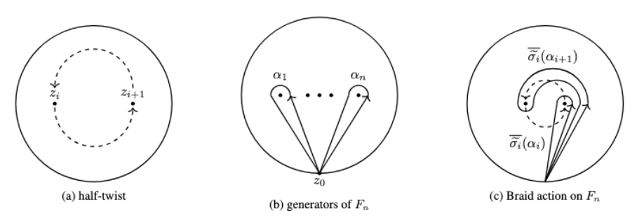
Figure 2: Settings for analytic construction

3.3 Multiplicative middle convolution

In order to formulate the multiplicative middle convolution for KZ equation, first we recall the definition of the additive middle convolution for KZ-type equation [16]. We consider the additive middle convolution of KZ-type equation in the $z_{0}$-direction. Take a fundamental matrix solution $\mathcal{U}(z_{0},z_{1},\dots,z_{n})$. As a function of a single variable $z_{1}$, $\mathcal{U}$ satisfies the ordinary differential equation

$$\frac{\partial u}{\partial z_{0}}=\left(\sum_{j=1}^{n}\frac{A_{0j}}{z_{0}-z_{j}}\right)u,$$ (3)

in $x_{1}$. This is the restriction of 3 in $z_{0}$-direction. The fundamental solution matrix of this equation is given as follows.

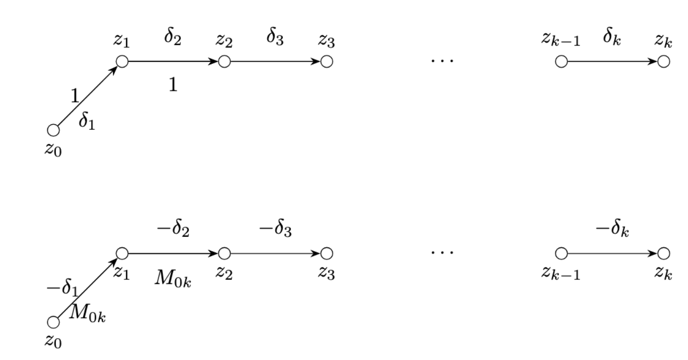
Figure 3: settings for path of analytic continutation

Let $l\in\mathbb{C}$ be a parameter. Define the matrix function

$$\mathcal{V}(z_{0},z_{1},\dots,z_{n})=\left(\int_{\Delta_{k}}\frac{\mathcal{U}(t,z_{1},\dots,z_{n})}{t-z_{j}}(t-z_{0})^{\lambda}dt\right)_{1\leq j,\ k\leq n},$$ (4)

where $\Delta_{k}$ ($1\leq k\leq n$) are defined as follows. Let $\delta_{k},k=0,\dots,n$ be the path from $z_{k}$ to $z_{k+1}$, and the loop $\alpha_{k}$ be the paths that satisfy

$$\begin{array}[]{clc}\alpha_{0}=&\delta_{0}(1-\lambda)&\\ \alpha_{k}=&(\delta_{0}+\dots+\delta_{k})(1-M_{0k})&k=1,\dots,n\end{array}.$$

Then, $\Delta_{k}=[\alpha_{k},\alpha_{0}]=\alpha_{k}\alpha_{0}\alpha_{k}^{-1}\alpha_{0}^{-1}$. By the linearity of integral, this solution space can be regarded as a vector space with the integration paths, $\Delta_{1},\dots,\Delta_{n}$, serving as its basis. We will specify them in the next section. It is shown that $\mathcal{V}$ satisfies the ordinary differential equation

$$\frac{\partial v}{\partial z_{0}}=\left(\sum_{j=1}^{n}\frac{B_{0j}}{z_{0}-z_{j}}\right)v,$$ (5)

in $z_{0}$, where $B_{0j}$ ($1\leq j\leq n$) are constant matrices of size $nN$ given by

$$B_{0j}=\begin{pmatrix}0&\cdots&0&\cdots&0\\ \vdots&\ddots&\vdots&\ddots&\vdots\\ A_{01}&\cdots&A_{0j}+\lambda&\cdots&A_{0n}\\ \vdots&\ddots&\vdots&\ddots&\vdots\\ 0&\cdots&0&\cdots&0\end{pmatrix}.$$ (6)

Equation 5 is called the convolution equation of 2 with parameter $\lambda$. Haroaka showed in [15, 16] that the ordinary differential equation can be prolonged to a Pfaffian system

$$d\nu=\left(\sum_{0\leq i<j\leq n}B_{ij}d\log(z_{i}-z_{j})\right)\nu,$$ (7)

in $(z_{0},z_{2},\dots,z_{n})$ with constant matrices $B_{ij}$ which are uniquely determined. We call the system (7) the convolution system of (3) in $z_{0}$-direction with parameter $\lambda$.

The basis of the solution space can be chosen as follows.

$$(\Delta_{1}\dots\Delta_{n}):=(\delta_{1}\dots\delta_{n})P$$

Here, $P$ is defined as follows to represent the twisted cycles.

$$P=\begin{pmatrix}(1-\lambda)(1-M_{02})&(1-\lambda)(1-M_{03})&\dots&(1-\lambda)(1-M_{0n})\\ &(1-\lambda)(1-M_{03})&&\vdots\\ &&\ddots&\vdots\\ &&&(1-\lambda)(1-M_{0n})\end{pmatrix}$$ (8)

Then, the monodromy matrices $N_{ij}$ with respect to this basis results in the following form.

$\begin{array}[]{cc}(\sigma_{ij*}\Delta_{1}\dots\sigma_{ij*}\Delta_{n})&=(\sigma_{ij*}\delta_{1}\dots\sigma_{ij*}\delta_{n})P\\ &=(\delta_{1}\dots\delta_{n})X(\sigma_{ij})P\\ &=(\delta_{1}\dots\delta_{n})PN_{ij}\\ &=(\Delta_{1}\dots\Delta_{n})N_{ij}\end{array}$

Here, $X(\sigma_{ij})$ satisfies $(\sigma_{ij*}\delta_{1}\dots\sigma_{ij*}\delta_{n})=(\delta_{1}\dots\delta_{n})X(\sigma_{ij}).$

Theorem 3.5 (Haraoka [16] Theorem 5.2).

Let $n$ and $N$ be positive integers, and let $V$ be a $N$-dim linear space over $\mathbb{C}$. We assume that $\lambda\in\mathbb{C}^{\times}$.

For the following anti-homomorphism, with generator of $P_{n+1}$, $\widetilde{\sigma_{ij}}(0\leq i<j\leq n)$,

$$\begin{array}[]{cccc}\widetilde{\rho}\colon&P_{n}&\stackrel{{\scriptstyle}}{{\longrightarrow}}&\text{GL}(V)\\ &\rotatebox{90.0}{$\in$}&&\rotatebox{90.0}{$\in$}\\ &\widetilde{\sigma_{ij}}&\longmapsto&M_{ij}\end{array},$$

we can obtain the following new anti-homomorphism $\rho^{H}_{\lambda}$ , with generator of $P_{n+1}$, $\widetilde{\sigma_{ij}},(0\leq i<j\leq n)$,

$\widetilde{\rho}^{\mathrm{H}}_{\lambda}$.

$$\begin{array}[]{cccc}\widetilde{\rho}^{\mathrm{H}}_{\lambda}\colon&P_{n}&\stackrel{{\scriptstyle}}{{\longrightarrow}}&\text{GL}(V^{\oplus n})\\ &\rotatebox{90.0}{$\in$}&&\rotatebox{90.0}{$\in$}\\ &\sigma_{ij}&\longmapsto&N_{ij}\end{array}$$

where ,$N_{ij}$ is defined as follows.

For $i=0$

$$N_{0j}:=\left(\begin{array}[]{ccccccc}1&&&&&&\\ &\ddots&&&&&\\ &&1&&&&\\ \lambda(M_{01}-1)&\cdots&\lambda(M_{0,j-2}-1)&\lambda M_{0j-1}&(M_{0j}-1)&\cdots&(M_{0n}-1)\\ &&&&1&&\\ &&&&&\ddots&\\ &&&&&&1\end{array}\right).$$

For $i>0$

$$N_{ij}:=\left(\begin{array}[]{ccc}M_{ij}^{\oplus(i-2)}&&\\ &N_{ij}^{{}^{\prime}}&\\ &&M_{ij}^{\oplus(n-j)}\end{array}\right).$$

Here, for $k=i+1,\dots,j-1$,we defined the following notations.

$$\begin{array}[]{cc}N_{ij}^{{}^{\prime}}\ =&\left(\begin{array}[]{ccccc}M_{0j}M_{ij}&X_{i+1}&\cdots&X_{j-1}&M_{0j}M_{ij}(1-M_{0j})\\ &M_{0i}^{-1}M_{ij}M_{0j}&&&\\ &&\ddots&&\\ &&&M_{0i}^{-1}M_{ij}M_{0j}&\\ M_{ij}(1-M_{0i})&Y_{i+1}&\cdots&Y_{j-1}&M[i,j,0]\\ \end{array}\right),\end{array}$$

$$\begin{array}[]{cc}X_{k}\ =&(M_{0j}M_{ij}-M_{1i}^{-1}M_{ij}M_{0j})(1-M_{0k}),\\ Y_{k}\ =&M_{ij}(1-M_{0i})(1-M_{0k}),\\ M[i,j,0]\ =&M_{ij}-M_{ij}M_{0j}+M_{0j}M_{ij}M_{0i}.\end{array}$$

Haraoka’s convolution is defined analytically, but it can also be defined on any field $\bm{k}$ as a method of constructing a new anti-representation $(N_{ij})_{0\leq i<j\leq n}$ of $P_{n}$ from the anti-representation $(M_{ij})_{0\leq i<j\leq n}$ of $P_{n+1}$. Therefore, we define a new method of constructing the anti-representation of $P_{n+1}$ on any field $\bm{k}$ and call it Haraoka’s convolution.

Definition 3.6 (Haraoka’s convolution).

Let $n$ and $N$ be positive integers, and let $V$ be a linear space $N$-dim over $\bm{k}$. In addition, we assume that $l\in\bm{k}^{\times}$. Then, for the following anti-homomorphism with the generator of $P_{n+1},\ (\sigma_{ij})_{0\leq i<j\leq n}$

$$\begin{array}[]{cccc}\rho\colon&P_{n+1}&\stackrel{{\scriptstyle}}{{\longrightarrow}}&\text{GL}(V)\\ &\rotatebox{90.0}{$\in$}&&\rotatebox{90.0}{$\in$}\\ &\widetilde{\sigma_{ij}}&\longmapsto&M_{ij}\end{array},$$

we define the anti-homomorphism of $P_{n}$ with the generator $(\widetilde{\sigma_{ij}})_{0\leq i<j\leq n}$, $\widetilde{\rho}^{\mathrm{H}}_{\lambda}$ as follows and call it as Haraoka’s convolution..

$$\begin{array}[]{cccc}\widetilde{\rho}^{\mathrm{H}}_{\lambda}\colon&P_{n}&\stackrel{{\scriptstyle}}{{\longrightarrow}}&\text{GL}(V^{\oplus n})\\ &\rotatebox{90.0}{$\in$}&&\rotatebox{90.0}{$\in$}\\ &\widetilde{\sigma_{ij}}&\longmapsto&N_{ij}\end{array}$$

See [16].

We can define the action of $\widetilde{\rho^{H}_{\lambda}}$ on the quotient space $\mathbb{C}^{Nn}/(K+L)$, So, we define $\bar{\widetilde{\rho^{H}_{\lambda}}}$ as the action of $\widetilde{\rho^{H}_{\lambda}}$ on $\mathbb{C}^{Nn}/(K+L)$.

It is shown in [10] that, under some generic condition, we can construct irreducible representation if the original representation is irreducible.

Remark 3.7.

The middle convolution, antirepresentation of $P_{n+1}$, is extended to $B_{n+1}$.

4 Katz-Long-Moody construction and multiplicative middle convolution

4.1 the Haraoka-Long natural transformation

The first main result is an isomorphism between the restriction of the twisted LM construction to $P_{n+1}$ and Haraoka’s convolution. Hereafter, $P_{n+1}$ shall be identified to $F_{n}\rtimes P_{n}$ as follows.

$$\begin{array}[]{cccc}&P_{n+1}&\stackrel{{\scriptstyle}}{{\longrightarrow}}&F_{n}\rtimes P_{n}\\ &\rotatebox{90.0}{$\in$}&&\rotatebox{90.0}{$\in$}\\ &\sigma_{ij}&\longmapsto&\left\{\begin{array}[]{ll}x_{j}&i=0\\ \sigma_{ij}&i>0\end{array}\right.\end{array}$$

With this identification, the twisted LM construction for $P_{n+1}$ can be rewritten as follows.

$$\begin{array}[]{ccccll}\rho\colon&F_{n}\rtimes P_{n}&\stackrel{{\scriptstyle}}{{\longrightarrow}}&\mathrm{GL}(V)&\\ &\rotatebox{90.0}{$\in$}&&\rotatebox{90.0}{$\in$}&\\ &x_{j}&\longmapsto&\rho(\sigma_{ij})&i=0\\ &\sigma_{ij}&\longmapsto&\rho(\sigma_{ij})&i>0\end{array}$$

we re-write as

$$\rho^{\mathrm{LM}}_{\lambda}(\sigma_{ij}):=\left\{\begin{array}[]{ll}\rho^{\mathrm{DR}}_{\lambda}(x_{j})&i=0\\ \rho^{\mathrm{LM}}_{\lambda}(\sigma_{ij})&i>0\end{array}\right.$$

Note that the twisted LM construction is a way of constructing representations of $P_{n+1}$, while the Haraoka’s convolution is a way of constructing the antirepresentation of $P_{n+1}$. In constructing these isomorphisms, we define anti-isomorphisms of groups as follows.

Definition 4.1 (group anti-isomorphism $\psi^{op}$).

For group $G$, we define antiisomorphism $\mathrm{inv}$ as $\mathrm{inv}\colon G\ni g\mapsto g^{-1}\in G$.

For group isomorphism $\psi\colon G\longrightarrow H$, we define anti-isomorphism $\psi^{op}\colon G\longrightarrow H$ as

$$\psi^{op}:=\psi\circ\mathrm{inv}$$

. In the same manner,
for antiisomorphism $\eta^{\mathrm{anti}}\colon G\longrightarrow H$, we define isomorphism $(\eta^{\mathrm{anti}})^{op}\colon G\longrightarrow H$ as

$$(\eta^{\mathrm{anti}})^{op}:=\eta^{\mathrm{anti}}\circ\mathrm{inv}.$$

Lemma 4.2.

For generator $B_{n}$, $(\sigma_{i})$, we define $\widetilde{\sigma_{i}}:=\sigma_{i}^{-1}$.

Here, we assume that

$$\sigma_{ij} :=\sigma_{i}\cdots\sigma_{j-2}(\sigma_{j-1})^{2}(\sigma_{j-2}^{-1}\cdots\sigma_{i}^{-1})$$

$$\widetilde{\sigma_{ij}} :=\widetilde{\sigma_{i}}\cdots\widetilde{\sigma_{j-2}}(\widetilde{\sigma_{j-1}})^{2}(\widetilde{\sigma_{j-2}}^{-1}\cdots\widetilde{\sigma_{i}}^{-1}),$$

then $(\sigma_{ij})$, $(\widetilde{\sigma_{ij}})$ are both generators of $P_{n+1}$.

Besides, the following proposition holds.

$$\rho^{op}(\widetilde{\sigma_{ij}})=\rho(\sigma_{ij}),$$

$$\begin{array}[]{cccccc}\rho^{op}\colon&P_{n+1}&\stackrel{{\scriptstyle\mathrm{inv}}}{{\longrightarrow}}&P_{n+1}&\stackrel{{\scriptstyle\rho}}{{\longrightarrow}}&\mathrm{GL}(V)\\ &\rotatebox{90.0}{$\in$}&&\rotatebox{90.0}{$\in$}&&\rotatebox{90.0}{$\in$}\\ &{\widetilde{\sigma_{ij}}}&\longmapsto&\sigma_{ij}&\longmapsto&\rho(\sigma_{ij})\end{array}$$

.

Theorem 4.3 (main result).

For a group homomorphism $\rho\colon P_{n+1}\longrightarrow\mathrm{GL}(V)$, let $\rho_{\lambda}^{\mathrm{LM}}$ be a generalized LM of $\rho$ for the generator $(\sigma_{ij})$, let $(\rho^{op})_{\lambda}^{\mathrm{H}}$ be a Haraoka’s convolution of $\rho^{op}$ for the generator $(\widetilde{\sigma_{ij}})$. Then we have

$$(\rho_{\lambda}^{\mathrm{LM}})^{op}=(\rho^{op})_{\lambda}^{\mathrm{H}}.$$

$$\begin{array}[]{ccc}\rho&\longrightarrow&\rho^{LM}_{\lambda}\\ \rotatebox{90.0}{$\longleftarrow$}&\circlearrowright&\rotatebox{90.0}{$\longleftarrow$}\\ \rho^{\operatorname{op}}&\longrightarrow&(\rho^{LM}_{\lambda})^{\operatorname{op}}\end{array}$$

Proof.

When we have$\rho(\sigma_{ij})=\rho^{op}(\widetilde{\sigma_{ij}})$, we will prove that $(\rho_{\lambda}^{\mathrm{LM}})^{op}(\widetilde{\sigma_{ij}})=(\rho^{op})_{\lambda}^{\mathrm{H}}(\widetilde{\sigma_{ij}})$. Here we divide into the following two cases; (1) for $i=1$, and (2) for $i>1$. Then we define the symbols as follows. $\rho^{op}(\widetilde{\sigma_{ij}})=M_{ij}$, and $(\rho^{op})_{\lambda}^{\mathrm{H}}(\widetilde{\sigma_{ij}})=N_{ij}$. When it is obvious from the context, we abbreviate $[n],[n]$.

(1) For $i=0$

By the representation of $\rho^{LM}_{\lambda}$ and $\rho^{H}_{\lambda}$ and the lemma 4.2, the following claim follows immediately.

$$(\rho^{op}(\widetilde{\sigma_{0j}}))_{\lambda}^{\mathrm{H}}= \left(\begin{array}[]{ccccccc}1&&&&&&\\ &\ddots&&&&&\\ &&1&&&&\\ \lambda(M_{01}-1)&\cdots&\lambda(M_{0j-1}-1)&lM_{0j}&(M_{0,j+1}-1)&\cdots&(M_{0n}-1)\\ &&&&1&&\\ &&&&&\ddots&\\ &&&&&&1\end{array}\right)$$

$$= (\rho_{\lambda}^{\mathrm{LM}})(\sigma_{0j})=(\rho_{\lambda}^{\mathrm{LM}})^{op}(\widetilde{\sigma_{0j}}).$$

In the last equation follows from $x_{j}=\widetilde{x_{j}}$.

(2) For $i>0$

Take any $n>2$. By computation of the elements of the matrices and by mathematical induction about $i$, we show that

$$(\rho_{\lambda}^{\mathrm{LM}})^{op}(\widetilde{\sigma_{ij}})=(\rho^{op}(\widetilde{\sigma_{ij}}))_{\lambda}^{\mathrm{H}}.$$

That is,we show that

1. For any $i$, it follows that $(\rho_{\lambda}^{\mathrm{LM}})^{op}(\sigma_{i,i+1})=(\rho^{op})_{\lambda}^{\mathrm{H}}(\widetilde{\sigma_{i,i+1}})$.

2. For any $i+1,j$, we assume that $(\rho_{\lambda}^{\mathrm{LM}})^{op}(\sigma_{i+1,j})=(\rho^{op})_{\lambda}^{\mathrm{H}}(\widetilde{\sigma_{i+1,j}})$. Then it follows that $(\rho_{\lambda}^{\mathrm{LM}})^{op}(\sigma_{i,j})=(\rho^{op})_{\lambda}^{\mathrm{H}}(\widetilde{\sigma_{i,j}})$.

1. The proof is based on the computation of the components of the matrix.

$$\begin{array}[]{cl}&(\rho^{\mathrm{LM}}_{\lambda})^{op}(\widetilde{\sigma_{i,i+1}})=\rho^{\mathrm{LM}}_{\lambda}(\sigma_{i}^{2})=s_{i}^{\oplus n}\cdot\left(\begin{array}[]{ccc}I_{N(i-1)}&&\\ &R_{i}&\\ &&I_{N(n-i-1)}\end{array}\right)\cdot s_{i}^{\oplus n}\cdot\left(\begin{array}[]{ccc}I_{N(i-1)}&&\\ &R_{i}&\\ &&I_{N(n-i-1)}\end{array}\right)\\ &=(s_{i}^{2})^{\oplus n}\cdot\left(\begin{array}[]{ccc}I_{N(i-1)}&&\\ &\Theta_{i}(R_{i})&\\ &&I_{N(n-i-1)}\end{array}\right)\cdot\left(\begin{array}[]{ccc}I_{N(i-1)}&&\\ &R_{i}&\\ &&I_{N(n-i-1)}\end{array}\right)\\ &=(s_{i}^{2})^{\oplus n}\cdot\left(\begin{array}[]{ccc}I_{N(i-1)}&&\\ &\Theta_{i}(R_{i})\cdot R_{i}&\\ &&I_{N(n-i-1)}\end{array}\right)\\ &=\left(\begin{array}[]{ccc}\rho(\sigma_{i}^{2})^{\oplus(i-1)}&&\\ &\rho(\sigma_{i}^{2})^{\oplus 2}\cdot\Theta_{i}(R_{i})\cdot R_{i}&\\ &&\rho(\sigma_{i}^{2})^{\oplus(n-i-1)}\end{array}\right)\\ &=\left(\begin{array}[]{ccc}\rho^{op}(\widetilde{\sigma_{i}}^{2})^{\oplus(i-1)}&&\\ &\rho(\sigma_{i}^{2})^{\oplus 2}\cdot\Theta_{i}(R_{i})\cdot R_{i}&\\ &&\rho^{op}(\widetilde{\sigma_{i}}^{2})^{\oplus(n-i-1)}\end{array}\right)\\ &=\left(\begin{array}[]{ccc}{M_{i,i+1}}^{\oplus(i-1)}&&\\ &\rho(\sigma_{i}^{2})^{\oplus 2}\cdot\Theta_{i}(R_{i})\cdot R_{i}&\\ &&{M_{i,i+1}}^{\oplus(n-i-1)}\end{array}\right).\end{array}$$

$$\begin{array}[]{cl}\rho(\sigma_{i}^{2})^{\oplus 2}\cdot\Theta_{i}(R_{i})\cdot R_{i}&=\rho(\sigma_{i}^{2})^{\oplus 2}\cdot\begin{pmatrix}0&\theta_{i}(g_{i})\\ 1&1-\theta_{i}(g_{i+1})\\ \end{pmatrix}\cdot\begin{pmatrix}0&g_{i}\\ 1&1-g_{i+1}\\ \end{pmatrix}\\ &=\rho(\sigma_{i}^{2})^{\oplus 2}\cdot\begin{pmatrix}\theta_{i}(g_{i})&\theta_{i}(g_{i})(1-g_{i+1})\\ 1-\theta_{i}(g_{i+1})&g_{i}+(1-\theta_{i}(g_{i+1}))(1-g_{i+1})\\ \end{pmatrix}\\ &=\begin{pmatrix}\rho(x_{i+1})\cdot\rho(\sigma_{i}^{2})&\rho(x_{i+1})\rho(\sigma_{i}^{2})(1-\rho(x_{i+1}))\\ \rho(\sigma_{i}^{2})\cdot(1-\rho(x_{i}))&\rho(\sigma_{i}^{2})\cdot(1-\rho(x_{i+1})+\rho(x_{i})\rho(x_{i+1}))\\ \end{pmatrix}\\ &=\begin{pmatrix}M_{0,i+1}M_{i,i+1}&M_{0i+1}M_{i,i+1}(1-M_{0,i+1})\\ M_{i,i+1}(1-M_{0i})&M[i,i+1,0]\\ \end{pmatrix}\end{array}.$$

Then, $(\rho^{\mathrm{LM}}_{\lambda})^{op}(\widetilde{\sigma_{i,i+1}})=N_{i,i+1}=(\rho^{op})_{\lambda}^{\mathrm{H}}(\widetilde{\sigma_{i,i+1}})$ holds.
2. For $1<i<i+1<j\leq n$, we assume that $(\rho^{op})_{\lambda}^{\mathrm{H}}(\widetilde{\sigma_{i+1,j}})=(\rho^{\mathrm{LM}}_{\lambda})^{op}(\widetilde{\sigma_{i+1,j}})$.Under the assumption, it suffices to show that $(\rho^{op})_{\lambda}^{\mathrm{H}}(\widetilde{\sigma_{i,j}})=(\rho^{\mathrm{LM}}_{\lambda})^{op}(\widetilde{\sigma_{i,j}})$.

$$\begin{array}[]{cl}RHS=(\rho^{\mathrm{LM}}_{\lambda})^{op}(\widetilde{\sigma_{i,j}})&=(\rho^{\mathrm{LM}}_{\lambda})^{op}(\widetilde{\sigma_{i}^{-1}})\cdot(\rho^{\mathrm{LM}}_{\lambda})^{op}(\widetilde{\sigma_{i+1,j}})\cdot(\rho^{\mathrm{LM}}_{\lambda})^{op}(\widetilde{\sigma_{i}})\\ &=(\rho^{\mathrm{LM}}_{\lambda})(\sigma_{i}^{-1})\cdot(\rho^{op})_{\lambda}^{\mathrm{H}}{(\widetilde{\sigma_{i+1,j}})}\cdot(\rho^{\mathrm{LM}}_{\lambda})(\sigma_{i})\end{array}$$

So, we show that

$$\rho^{\mathrm{LM}}_{\lambda}(\sigma_{i}^{-1})\cdot N_{i+1,j}\cdot\rho^{\mathrm{LM}}_{\lambda}(\sigma_{i})=LHS=N_{i,j}.$$

$$\begin{array}[]{ll}&\rho^{\mathrm{LM}}_{\lambda}(\sigma_{i}^{-1})\cdot N_{i+1,j}\cdot\rho^{\mathrm{LM}}_{\lambda}(\sigma_{i})\\ =&\begin{pmatrix}(s_{i}^{-1})^{\oplus(i-1)}&&\\ &R_{i}^{-1}(s_{i}^{-1})^{\oplus 2}&\\ &&(s_{i}^{-1})^{\oplus(n-i-1)}\end{pmatrix}\cdot N_{i+1,j}\cdot\begin{pmatrix}s_{i}^{\oplus(i-1)}&&\\ &R_{i}s_{i}^{\oplus 2}&\\ &&s_{i}^{\oplus(n-i-1)}\end{pmatrix}\\ =&\begin{pmatrix}(s_{i}^{-1})^{\oplus(i-1)}&&\\ &R_{i}^{-1}(s_{i}^{-1})^{\oplus 2s}&\\ &&(s_{i}^{-1})^{\oplus(n-i-1)}\end{pmatrix}\cdot\left(\begin{array}[]{ccc}(M_{i+1,j})^{\oplus i}&&\\ &N_{i+1,j}^{{}^{\prime}}&\\ &&M_{i+1,j}^{\oplus(n-j)}\end{array}\right)\\ &\cdot\begin{pmatrix}s_{i}^{\oplus(i-1)}&&\\ &R_{i}s_{i}^{\oplus 2}&\\ &&s_{i}^{\oplus(n-i-1)}\end{pmatrix}\\ =&\begin{pmatrix}(s_{i}^{-1}M_{i+1,j}s_{i})^{\oplus(i-1)}&&\\ &X&\\ &&(s_{i}^{-1}M_{i+1,j}s_{i})^{\oplus(n-j)}\end{pmatrix}\\ =&\begin{pmatrix}{M_{ij}}^{\oplus(i-1)}&&\\ &X&\\ &&{M_{ij}}^{\oplus(n-j)}\end{pmatrix}=N_{i,j}.\end{array}$$

Here we denote X as follows.

$\begin{array}[]{rl}X&=\begin{pmatrix}R_{i}^{-1}\cdot(s_{i}^{-1})^{\oplus 2}&\\ &(s_{i}^{-1})^{\oplus(j-i-2)}\end{pmatrix}\begin{pmatrix}M_{i+1,j}&\\ &N_{i+1,j}^{{}^{\prime}}\end{pmatrix}\begin{pmatrix}s_{i}^{\oplus 2}\cdot R_{i}&\\ &s_{i}^{\oplus(j-i-2)}\end{pmatrix}\\ =&\begin{pmatrix}R_{i}^{-1}\cdot(s_{i}^{-1})^{\oplus 2}&\\ &(s_{i}^{-1})^{\oplus(j-i-2)}\end{pmatrix}\begin{pmatrix}M_{i+1,j}&\\ &N_{i+1,j}^{{}^{\prime}}\end{pmatrix}\begin{pmatrix}s_{i}^{\oplus 2}\cdot R_{i}&\\ &s_{i}^{\oplus(j-i-2)}\end{pmatrix}\\ =&\begin{pmatrix}(g_{i+1}-1)g_{i}^{-1}s_{i}^{-1}&s_{i}^{-1}&\\ g_{i}^{-1}&0&\\ &&(s_{i}^{-1})^{\oplus(j-i-2)}\end{pmatrix}\\ \cdot&\left(\begin{array}[]{cccccc}M_{i+1,j}&&&&&\\ &M_{0j}M_{i+1,j}&X_{i+2}&\cdots&X_{j-1}&M_{0j}M_{i+1,j}(1-M_{0j})\\ &&M_{0,i+1}^{-1}M_{i+1,j}M_{0j}&&&\\ &&&\ddots&&\\ &&&&M_{0,i+1}^{-1}M_{i+1,j}M_{0j}&\\ &M_{i+1,j}(1-M_{0,i+1})&Y_{i+2}&\cdots&Y_{j-1}&M[i+1,j,0]\\ \end{array}\right)\\ \cdot&\begin{pmatrix}o&s_{i}g_{i}&\\ s_{i}&s_{i}(1-g_{i+1})&o\\ &&s_{i}^{\oplus(j-i-2)}\\ \end{pmatrix}\\ &=N_{ij}^{{}^{\prime}}\end{array}$

Due to the foregoing argument,

1. 

for any $i$,$(\rho_{\lambda}^{\mathrm{LM}})^{op}(\sigma_{i,i+1})=(\rho^{op})_{\lambda}^{\mathrm{H}}(\widetilde{\sigma_{i,i+1}})$,

2. 

for any $i+1,j$, if $(\rho_{\lambda}^{\mathrm{LM}})^{op}(\sigma_{i+1,j})=(\rho^{op})_{\lambda}^{\mathrm{H}}(\widetilde{\sigma_{i+1,j}})$ is true, then $(\rho_{\lambda}^{\mathrm{LM}})^{op}(\sigma_{i,j})=(\rho^{op})_{\lambda}^{\mathrm{H}}(\widetilde{\sigma_{i,j}})$.

With mathematical induction in $i$ proved the statement of case (2).

Finally, by (1),(2), it follows that

$$(\rho_{\lambda}^{\mathrm{LM}})^{op}=(\rho^{op})_{\lambda}^{\mathrm{H}}.$$

∎

4.2 Correspondence with the two settings

Here we discuss the differences in the settings between the algebraic construction method (KLM) and the analytic construction method (MC), which are essential for establishing the correspondence between them.

The KLM construction method yields representations consisting of group homomorphisms, whereas the MC method produces anti-representations consisting of group antihomomorphisms. Moreover, we note that the orientations of paths defining the generators of the fundamental groups of the domains differ between the two methods. This difference in path orientation causes a change in the generators of the pure braid group.

4.3 irreducibility

In [16] theorem 5.7, it is mentioned that middle convolution can produce irreducible representation if we assume that $M_{0j}$ is irreducible. By combining the theorem and the Haraoka-Long natural transformatin, we can obtain irredicible representation of $F_{n}\rtimes B_{n}$ via the Katz-Long-Moody construction, if we assume that $\rho$ is irreducible.

5 Unitarity

5.1 Monodromy invariant Hermitian form

In this section, we discuss the unitarity of the braid representations, which is our second result. In this section, we fix $\bm{k}$ as $\mathbb{C}$ and denote $X^{{\dagger}}$ be the adjoint matrix of $X$.

Definition 5.1 (Unitarity of representation [27]).

Let $\rho\colon G\longrightarrow GL(V)$ be unitary relative to $H$ if there exists a nondegenerate Hermitian matrix $H$ such that $\rho(g)^{{\dagger}}H\rho(g)=H\text{ holds for any }g\in G.$

In [27], Long proved that if $\rho$ is unitary, so is $\rho^{LM}_{s}$ for some generic value $s$, according the method by Delingne-Mostow[9]. Here, $\rho^{LM}_{s}(\sigma_{i}):=s\cdot\rho^{LM}(\sigma_{i})$.

We extend the result and show that unitarity is preserved by Katz-Long-Moody construction under some conditions. It also follows that multiplicative middle convolution of KZ-type equations preserves unitarity. First, as mentioned in the introduction, we construct a Hermitian matrix, not necessarily nondegenerate, that satisfies the unitarity condition. Finally, we show the algorithm to obtain the condition under which this Hermitian matrix becomes nondegenerate.

Theorem 5.2.

Assume that there exists a Hermitian matrix $H$ that satisfies $\rho(\beta)^{{\dagger}}H\rho(\beta)$ for any $\beta\in F_{n}\rtimes B_{n}$. Then $\rho^{LM}_{\lambda}$ is unitary relative to $\widetilde{H}$.

Here, we define

$$(\widetilde{H})_{jk}:=h_{jk}=\lambda^{jk}H(g_{j}^{-1}-\lambda_{jk}I)(g_{k}-1),$$

$$\lambda^{jk}=\left\{\begin{array}[]{ll}\lambda^{-\frac{1}{2}}&j\leq k\\ \lambda^{\frac{1}{2}}&j>k\end{array}\right.,\ \lambda_{jk}=\left\{\begin{array}[]{ll}\lambda&j=k=i\\ 1&otherwise\end{array}\right.$$

Furthermore, we get the following theorem.

Theorem 5.3.

$K$ and $L$ is $\widetilde{H}$ invariant. Therefore, $\bar{\rho^{KM}_{\lambda}}$ is unitary relative to the Hermitian matrix defined by the action of $\widetilde{H}$ on $V/(K+L)$.

Proof of theorem 5.2.

If $\rho$ is unitary, there is a Hermitian matrix $H$ which satisfies $\overline{{}^{t}\rho(\sigma_{i})}H\rho(\sigma_{i})=H$. For such Hermetian Matrix $H$, let $\widetilde{H}$ be the following matrix of size $Nn\times Nn$ defined as below.

$$(\widetilde{H})_{jk}:=h_{jk}=\lambda^{jk}H(g_{j}^{-1}-\lambda_{jk}I)(g_{k}-1)$$

Here, we defined $\lambda^{jk},\lambda_{jk}$ as follows.

$$\lambda^{jk}=\left\{\begin{array}[]{ll}\lambda^{-\frac{1}{2}}&j\leq k\\ \lambda^{\frac{1}{2}}&j>k\end{array}\right.,\ \lambda_{jk}=\left\{\begin{array}[]{ll}\lambda&j=k=i\\ 1&otherwise\end{array}\right.$$

Besides, we denote $(i,k)$-th elementof $\widetilde{G_{i}}$, $g_{ik}$ , as follows.

$$g_{ik}:=\lambda^{k}(g_{k}-\lambda_{k}I)$$

Here, we defined $\lambda^{k},\lambda_{k}$ as follows.

$$\lambda^{k}=\left\{\begin{array}[]{ll}\lambda&k\leq i\\ 1&k>i\end{array}\right.,\ \lambda_{k}=\left\{\begin{array}[]{ll}\lambda^{-1}&k=i\\ 1&otherwise\end{array}\right.$$

Then, for $G_{i},i=1,\cdots,n,$ we will show that

$$\begin{array}[]{cc}&(^{t}\overline{I+\widetilde{G_{i}}})\widetilde{H}(I+\widetilde{G_{i}})=\widetilde{H}\\ \iff&{}^{t}\overline{\widetilde{G_{i}}}\widetilde{H}+\widetilde{H}\widetilde{G_{i}}+(^{t}\overline{\widetilde{G_{i}}})\widetilde{H}\widetilde{G_{i}}=O\\ \end{array}$$

$$\begin{array}[]{cl}(k,l)\text{-th element of (LHS)}&={\sum_{s=1}^{n}}^{t}\overline{g_{sk}}h_{s,l}+\sum_{t=1}^{n}h_{k,t}g_{t,l}+\sum_{s=1}^{n^{t}}\overline{g_{sk}}\left\{\sum_{t=1}^{n}h_{s,t}g_{t,l}\right\}\\ &=^{t}\overline{g_{ik}}h_{i,l}+h_{k,i}g_{i,l}+^{t}\overline{g_{ik}}h_{i,i}g_{i,l}\\ &=^{t}\overline{h_{l,i}g_{ik}}+h_{k,i}g_{i,l}+^{t}\overline{g_{ik}}h_{i,i}g_{i,l}.\end{array}$$

For each term, the following equality holds.

$$\begin{array}[]{rl}h_{k,i}g_{i,l}=&\lambda^{ki}\lambda^{l}H(g_{k}^{-1}-\lambda_{ki})(g_{i}-I)(g_{l}-\lambda_{l})\end{array}$$

$$\begin{array}[]{rl}{}^{t}\overline{h_{l,i}g_{i,k}}=&{}^{t}\overline{\lambda^{li}\lambda^{k}H(g_{l}^{-1}-\lambda_{li})(g_{i}-1)(g_{k}-\lambda_{k})}\\ =&{}^{t}\overline{\lambda^{li}\lambda^{k}(^{t}\overline{g_{l}}-\lambda_{li})(^{t}\overline{g_{i}^{-1}}-I)(^{t}\overline{g_{k}^{-1}}-\lambda_{k})H}\\ =&\overline{\lambda^{li}\lambda^{k}}H\ ^{t}\overline{(^{t}\overline{g_{k}^{-1}}-\lambda_{k})}\ ^{t}\overline{(^{t}\overline{g_{i}}^{-1}-I)}\ ^{t}\overline{{}^{t}\overline{(g_{l}-\lambda_{li})}}\\ =&\overline{\lambda^{li}\lambda^{l}}H(g_{k}^{-1}-\overline{\lambda_{k})}(g_{i}^{-1}-I)(g_{l}-\lambda_{li})\end{array}$$

$$\begin{array}[]{rl}{}^{t}\overline{g_{ik}}h_{i,i}g_{i,l}=&{}^{t}\overline{\lambda^{k}(g_{k}-\lambda_{k}I)}\lambda^{ii}H(g_{i}^{-1}-\lambda)(g_{i}-I)\lambda^{l}(g_{l}-\lambda_{l}I)\\ =&\overline{\lambda^{k}}\lambda^{-\frac{1}{2}}\lambda^{l}(^{t}\overline{g_{k}}-\overline{\lambda_{k}})H(g_{i}^{-1}-\lambda)(g_{i}-I)(g_{l}-\lambda_{l}I)\\ =&\overline{\lambda^{k}}\lambda^{-\frac{1}{2}}\lambda^{l}H(g_{k}^{-1}-\overline{\lambda_{k}})(g_{i}^{-1}-\lambda)(g_{i}-I)(g_{l}-\lambda_{l}I)\end{array}$$

Consequently,

$$\begin{array}[]{cl}(k,l)\text{-th element of (LHS)}=&\lambda^{l}a_{1}g_{k}^{-1}g_{i}g_{l}+\overline{\lambda^{k}}a_{2}g_{k}^{-1}g_{i}^{-1}g_{l}-\lambda^{l}\lambda_{l}a_{1}g_{k}^{-1}g_{i}-\overline{\lambda^{k}}a_{3}g_{k}^{-1}g_{i}^{-1}\\ &-\{\lambda^{l}a_{1}+\overline{\lambda^{k}}a_{2}\}g_{k}^{-1}g_{l}+\{\overline{\lambda^{k}}a_{3}+\lambda^{l}\lambda_{l}a_{1}\}g_{k}^{-1}-\lambda^{l}a_{4}g_{i}g_{l}-\overline{\lambda_{k}}\overline{\lambda^{k}}a+2g_{i}^{-1}g_{l}\\ &+\lambda^{l}\lambda_{l}a_{4}g_{i}+\overline{\lambda^{k}}\overline{\lambda_{k}}a_{3}g_{i}^{-1}-\{\overline{\lambda^{k}}\overline{\lambda_{k}}a_{3}+\lambda^{l}\lambda_{l}a_{4}\},\end{array}$$

where $a_{1}=\lambda^{ki}-\lambda^{\frac{1}{2}}\overline{\lambda^{k}},a_{2}=\overline{\lambda^{li}}-\lambda^{-\frac{1}{2}}\lambda^{l},a_{3}=\overline{\lambda^{li}}\overline{\lambda_{li}}-\lambda^{ii}\lambda^{l}\lambda_{l},a_{4}=\lambda^{ki}\lambda_{ki}-\lambda^{\frac{1}{2}}\overline{\lambda^{k}}\overline{\lambda_{k}}.$

For $k,l<i$, $a_{1}=a_{2}=\lambda^{-\frac{1}{2}}-\lambda^{\frac{1}{2}}\lambda^{-1}=0,$ and $a_{3}=a_{4}=\lambda^{-\frac{1}{2}}\cdot 1-\lambda^{\frac{1}{2}}\lambda^{-1}\cdot 1=0.$

For $k,l>i$, $a_{1}=a_{2}=\lambda^{\frac{1}{2}}-\lambda^{\frac{1}{2}}\cdot 1=0,$ and $a_{3}=a_{4}=\lambda^{\frac{1}{2}}\cdot 1-\lambda^{\frac{1}{2}}\cdot 1\cdot 1=0.$

For $k,l=i$, $a_{1}=a_{2}=\lambda^{-\frac{1}{2}}-\lambda^{\frac{1}{2}}\lambda^{-1}=0,$ and $a_{3}=a_{4}=\lambda^{-\frac{1}{2}}\lambda-\lambda^{\frac{1}{2}}\lambda^{-1}\lambda=0.$

Thus, the $(k,l)$-element is identically zero.

For $S_{i},i=1,\cdots,n,$ we will show that

$${}^{t}\overline{S_{i}}\widetilde{H}S_{i}=\widetilde{H}$$

As in the case of $\rho^{LM}_{\lambda}(x_{j})$, the left-hand side is Hermitian, so it suffices to show the case where $k\leq l$ for $(k,l)$-components.

If $k,l\neq i,i+1$

$$\begin{array}[]{cl}(\operatorname{LHS})_{kl}&=s_{i}^{{\dagger}}(\lambda^{kl}H(g_{k}^{-1}-1)(g_{l}-1))s_{i}\\ &=\lambda^{kl}Hs_{i}^{-1}s_{i}(g_{k}^{-1}-1)(g_{l}-1)\\ &=(\widetilde{H})_{kl}.\end{array}$$

If $k\neq i,i+1$ and $l=i$,

$$\begin{array}[]{cl}(\operatorname{LHS})_{ki}=&s_{i}^{{\dagger}}(\lambda^{ki}H(g_{k}^{-1}-1)(g_{i}-1))s_{i}-\lambda^{k,i+1}Hs_{i}^{-1}(g_{k}^{-1}-1)(g_{i}-1)s_{i}\\ &+\lambda^{k,i+1}Hs_{i}-^{-1}(g_{k}^{-1}-1)(g_{i+1}-1)s_{i}\\ =&\lambda^{k,i}H(g_{k}^{-1}-1)(g_{i}-1)\\ =&(\widetilde{H})_{ki}.\end{array}$$

If $k\neq i,i+1$ and $l=i+1$,

$$\begin{array}[]{cl}(\operatorname{LHS})_{k,i+1}=&s_{i}^{{\dagger}}(\lambda^{ki}H(g_{k}^{-1}-1)(g_{i+1}-1))s_{i}+\lambda^{k,i}Hs_{i}^{-1}(g_{k}^{-1}-1)(g_{i}-1)s_{i}g_{i}\\ &-\lambda^{k,i+1}Hs_{i}-^{-1}(g_{k}^{-1}-1)(g_{i+1}-1)s_{i}g_{i+1}\\ =&\lambda^{k,i}H(g_{k}^{-1}-1)(g_{i+1}-1)\\ =&(\widetilde{H})_{k,i+1}.\end{array}$$

If $k=l=i$,

$$\begin{array}[]{cl}(\operatorname{LHS})_{i,i}=&s_{i}^{{\dagger}}(\lambda^{i+1,i+1}H(g_{i+1}^{-1}-\lambda)(g_{i+1}-1))s_{i}\\ =&\lambda^{i,i}H(g_{i}^{-1}-\lambda)(g_{i}-1)\\ =&(\widetilde{H})_{i,i}.\end{array}$$

If $k=i,l=i+1$,

$$\begin{array}[]{cl}(\operatorname{LHS})_{i,i}=&s_{i}^{{\dagger}}(\lambda^{i+1,i}H(g_{i+1}^{-1}-1)(g_{i}-1))s_{i}g_{i}+s_{i}^{{\dagger}}(\lambda^{i+1,i+1}H(g_{i+1}^{-1}-\lambda)(g_{i+1}-1))s_{i}(1-g_{i+1})\\ =&(\widetilde{H})_{i+1,i+1}.\end{array}$$

∎

Proof of theorem 5.3.

It suffice to show that (1) $\widetilde{H}K\subseteq K$ and (2) $\widetilde{H}L\subseteq L$.

$$\widetilde{H}=\lambda^{-\frac{1}{2}}\begin{pmatrix}g_{1}^{-1}-\lambda&g_{2}^{-1}-1&\cdots&g_{n}^{-1}-1\\ \lambda(g_{2}^{-1}-1)&g_{2}^{-1}-\lambda&\cdots&g_{n}^{-1}-1\\ \vdots&\vdots&\ddots&g_{n}^{-1}-1\\ \lambda(g_{1}^{-1}-1)&\lambda(g_{2}^{-1}-1)&\cdots&g_{n}^{-1}-\lambda\\ \end{pmatrix}H^{\oplus n}\begin{pmatrix}g_{1}-1&&\\ &\ddots&\\ &&g_{n}-1\\ \end{pmatrix}.$$

By the definition of $K$, $\widetilde{H}K=\bm{0}\subset K.$

$$\widetilde{H}=\widetilde{H}^{{\dagger}}=\begin{pmatrix}g_{1}^{{\dagger}}-1&&\\ &\ddots&\\ &&g_{n}^{{\dagger}}-1\\ \end{pmatrix}H^{\oplus n}\begin{pmatrix}\lambda g_{1}-1&g_{2}-1&\cdots&g_{n}-1\\ \lambda(g_{1}-1)&\lambda g_{2}-1&\cdots&g_{n}-1\\ \vdots&\vdots&\ddots&g_{n}-1\\ \lambda(g_{1}-1)&\lambda(g_{2}-1)&\cdots&\lambda g_{n}-1\\ \end{pmatrix}.$$

By the definition of $L$, $\widetilde{H}L=\bm{0}\subset L.$ ∎

5.2 Signature of the Hermitian form

Subsequently, we establish the signature of $\widetilde{H}$. Here, we introduce the following notation for convenience. For any matrix $X$ and for any regular matrix $A$, we define $X_{A}:=A^{{\dagger}}XA$ when we want to obtain the transformation that does not change the signature.

Remark 5.4.

The signature of $X_{A}$ is identical to the signature of the eigenvalues of $A$, with weight.

Let $U$ be a unitary matrix. Then, the set of the eigenvalues of $X_{U}$ is identical to the set of the eigenvalues of $X$, with weight.

In particular, when the entries of the matrix form a Hermitian form, we introduce the following notation. Let $A$ be a $p\times p$ Hermitian matrix and let $X$ be a $p\times q$ matrix, then we denote $A[X]$ as $X^{{\dagger}}AX$. Hereafter, whenever we consider unitary matrices, we assume that they have determinant one, i.e., they belong to the special unitary group, $SU(m)$. For simplicity, we will refer to these matrices just as unitary matrices.

5.2.1 Algorithm to determine signature of the Hermitian matrix

We construct the algorithm to determine the signature of $\tilde{H}$. Here we recursively apply block diagonalization method to the matrix $\widetilde{H}$ by considerting the matrix as $2\times 2$ block-matrix. However, a problem arises since the component matrices may not be invertible. To address this issue, we establish the following proposition concerning the the eigenvalues and eigenvectors of the component block matrices.

Let $A$ be a $n\times n$ block matrix, and $A_{kl}$ be the $(k,l)$-block element of $A$. Let $A$ be a Hermitian matrix. Namely, $A_{kl}^{{\dagger}}=A_{lk}$.

By assumption, $A_{ii}$ is a Hermitian matrix. So there is a unitary matrix which diagonalize $A_{ii}$. We define the unitary matrix $U_{i}$ as follows. Let $p_{i}$ be the number of the non-zero eigenvalues of $g_{i}$ with their multiplicity and let $\zeta^{i}_{k}$, $k=1,\dots,N$ be the eigenvalues of $g_{i}$, and $\zeta^{i}_{k}=0$ for $k=p_{i}+1,\dots,N$. Then we define $u^{i}_{k}\in\mathbb{C}^{N}$ as the eigenvector of the eigenvector $\zeta^{i}_{k}$, respectively. And we denote $U_{i}$ as $(u^{i}_{1}\ \dots\ u^{i}_{N})$. By the definition of $U_{i}$, the following lemma immediately follows.

Lemma 5.5.

Let $u_{i,1}$ be $(u^{i}_{1}\ \dots\ u^{i}_{p_{i}})$ and $u_{i,0}$ be $(u^{i}_{p_{i}+1}\ \dots\ u^{i}_{N})$. Then, $A_{ii}[U_{i}]=\begin{pmatrix}A_{ii}[u_{i,1}]&O\\ O&O\\ \end{pmatrix}$ holds. Here, $A_{ii}[u_{i,1}]$ is invertible.

We denote $u_{i,1}$ by $(u^{i}_{1}\dots u^{i}_{p_{i}})$. By using the basis, we can divide the $A_{11}$ into the following 4 blocks;

$\begin{array}[]{cl}A_{\widetilde{U}}=&\left(\begin{array}[]{ccc}A_{11}[u_{1,1}]&u_{1,1}^{{\dagger}}A_{12}&u_{11}^{{\dagger}}A_{11}u_{10}\\ A_{21}u_{1,1}&A_{22}&A_{21}u_{10}\\ u_{10}^{{\dagger}}A_{11}u_{11}&u_{10}^{{\dagger}}A_{12}u_{20}&A_{11}[u_{1,0}]\end{array}\right)\\ =&\left(\begin{array}[]{ccc}A_{11}[u_{1,1}]&u_{1,1}^{{\dagger}}A_{12}&O\\ A_{21}u_{1,1}&A_{22}&O\\ O&O&O\end{array}\right)\end{array}.$

Here we define

$\widetilde{U}:=\begin{pmatrix}u_{1,1}&&\\ &&u_{1,0}\\ &I_{N}&\\ \end{pmatrix}.$

Note that $A[u_{1,1}]$ is invertible. So we can diagonalize by $T:=\begin{pmatrix}I_{p_{1}}&-(A[u_{1,1}])^{-1}A[u_{2,1}]\\ O&I_{N}\end{pmatrix}$.

$$A_{\widetilde{U}T}=\begin{pmatrix}A_{11}[u_{1,1}]&O\\ O&A_{22}-(A[u_{1,1}])^{-1}[u_{11}^{{\dagger}}A_{21}]\end{pmatrix}$$

To block-diagonalize $A$, we first consider the case in which $A_{1,k}$ and $A_{k,1}$, $k=2,\dots,n$ are transformed into zero matrices by $A_{11}$. Namely, we consider

$$A=\begin{pmatrix}A_{11}&A_{12}&\dots&A_{1n}\\ A_{21}&A_{22}&\dots&A_{2n}\\ \vdots&&\ddots&\vdots\\ A_{n1}&A_{n2}&\dots&A_{nn}\end{pmatrix}\text{,\ as }\begin{pmatrix}A_{11}&X_{12}\\ X_{21}&A^{2}_{22}\\ \end{pmatrix}.$$

Subsequently, by applying this procedure recursively, $A^{2}_{22},A^{3}_{22}$ and so forth, we obtain a block-diagonalized matrix whose off-diagonal components become zero matrices.

To block-diagonalize $\widetilde{H}$, we introduce the following well-known lemma regarding a basis for the eigenspace corresponding to the zero eigenvalue of $H_{1}-H_{2}$ , where $H_{1}$ and $H_{2}$ are Hermitian matrices.

Lemma 5.6.

Let $H_{1},H_{2}$ be $p\times p$ Hermitian matrices, and let $\zeta_{1},\dots,\zeta_{p}$ be the eigenvalues of $H_{1}$. Let $U_{1}:=(u_{1}\dots u_{p})$ be the unitary matrix such that $H_{1}[U]=\operatorname{diag}(\zeta_{1},\dots\zeta_{p})$. Then, $H_{1}-H_{1}$ has eigenvalue 0 if and only if $H_{1}$ and $H_{2}$ share the same eigenvalue(s) and its eigenvector(s).

So, denote the shared pair of eigenvalue(s) and the eigenvector as $(\zeta_{q+1},u_{q+1}),\dots,(\zeta_{p},u_{p})$. Then, there is a unitary matrix $U_{2}:=(w_{1}\ \dots\ w_{q}\ u_{q+1}\ \dots\ u_{p})$ such that $w_{i},i=1,\dots,q$ are linear combinations of $u_{1},\dots,u_{q}$ and $U_{2}=U_{1}\operatorname{diag}(C,I_{q})$ for unitary $(p-q)\times(p-q)$ matrix $C$. Then,

$$(H_{1}-H_{2})[U_{1}]=\begin{pmatrix}u_{1,1}^{{\dagger}}(H_{1}-H_{2})u_{1,1}&u_{1,1}^{{\dagger}}(H_{1}-H_{2})u_{1,0}\\ u_{1,0}^{{\dagger}}(H_{1}-H_{2})u_{1,1}&u_{1,0}^{{\dagger}}(H_{1}-H_{2})u_{1,0}\end{pmatrix}=\begin{pmatrix}(H_{1}-H_{2})[u_{1,1}]&O\\ O&O\end{pmatrix},$$

where $u_{1,0}=(u_{1}\ \dots\ u_{q})$ and $u_{1,1}=(u_{q+1}\ \dots\ u_{p})$. Here, $(H_{1}-H_{2})[u_{1,1}]=\operatorname{diag}(\zeta_{1},\dots,\zeta_{q})-H_{2}[u_{1,1}C]$, and $(H_{1}-H_{2})[u_{1,1}]$ is invertible.

We iteratively apply this method to block-diagonalize $\widetilde{H}$. Here, we construct the finite sequences of matrices $\widetilde{H^{s}}$, $U^{s}$, $C^{s}$ for $s=1,\dots,n$ by the following way.

For $s=1$, $\widetilde{H^{1}}=\widetilde{H}$, $\widetilde{U^{1}}=U_{1}$, and $C^{1}=I_{N}$.

For $1\leq s\leq n-1$, we diagonalize $\widetilde{H^{s}}$ by the following procedure.

Diagonalize process (a):

Calculate the pairs of eigenvalues and the eigenvectors $(\zeta^{s}_{1},u^{s}_{1}),\dots,(\zeta^{s}_{q_{s}},u^{s}_{q_{s}}),(0,u^{s}_{q_{s}+1}),\dots,(0,u^{s}_{p_{s}})$ of $(\widetilde{H^{s}})_{11}$ where $(\widetilde{H^{s}})_{11}$ is $p_{s}\times p_{s}$ matrix and $\zeta_{1},\dots,\zeta_{q_{s}}$ are nonzero eigenvalues.

Diagonalize process (b):

Define $\widetilde{U^{s}}$ as $\begin{pmatrix}u^{s}_{1,1}&&\\ &&u^{s}_{1,0}\\ &I_{N}(n-s)&\end{pmatrix}$ where $u^{s}_{1,1}=(u^{s}_{1}\ \dots\ u^{s}_{q_{s}})$ and $u^{s}_{1,0}=(u^{s}_{q_{s}+1}\ \dots\ u^{s}_{p_{s}})$. Then, $\widetilde{H^{s}}_{\widetilde{U^{s}}}=\begin{pmatrix}\widetilde{H}^{s}_{11}[u^{s}_{11}]&{u^{s}_{11}}^{{\dagger}}\widetilde{H^{s}}_{12}&O\\ \widetilde{H^{s}}_{21}u^{s}_{11}&\widetilde{H^{s}}_{22}&O\\ O&O&O\end{pmatrix}$.

Diagonalize process (c):

$\left(\begin{array}[]{cc}\widetilde{H^{s}}_{11}[u^{s}_{11}]&{u^{s}_{11}}^{{\dagger}}\widetilde{H^{s}}_{12}\\ \widetilde{H^{s}}_{21}u^{s}_{11}&\widetilde{H^{s}}_{22}\\ \end{array}\right)$ is diagonalized by $T^{s}:=\begin{pmatrix}I_{p_{s}}&-(\widetilde{H^{s}}[\widetilde{U^{s}}])^{-1}{u^{s}_{11}}^{{\dagger}}(\widetilde{H^{s}})_{1,2}\\ O&I_{N}\end{pmatrix}$ and the result is

$$\begin{pmatrix}H^{s}_{11}&O&\cdots&O\\ O&H^{s}_{22}-{H^{s}_{12}}^{{\dagger}}(H^{s}_{11})^{-1}H^{s}_{12}&\cdots&H^{s}_{2,n}-{H^{s}_{12}}^{{\dagger}}(H^{s}_{11})^{-1}H^{s}_{1n}\\ \vdots&\vdots&\ddots&\vdots\\ O&H^{s}_{n,2}-{H^{s}_{1,n}}^{{\dagger}}(H^{s}_{11})^{-1}H_{12}&\cdots&A^{\lambda}_{n,n}-{H^{s}_{1n}}^{{\dagger}}(H_{11})^{-1}H^{s}_{1n}\end{pmatrix},$$

where $H^{s}_{kl}$ is $(k,l)$-block element of $\widetilde{H^{s}}$. Since $\widetilde{H^{s}}$ is a Hermitian matrix, $H_{kl}^{{\dagger}}=H_{lk}.$

Then we define $(n-1)\times(n-1)$ block matrix, $\widetilde{H^{(s+1)}}$ as

$$\begin{pmatrix}H_{22}-H_{12}^{{\dagger}}(H_{11})^{-1}H_{12}&\cdots&H_{2n}-H_{12}^{{\dagger}}(H_{11})^{-1}H_{1n}\\ \vdots&\ddots&\vdots\\ H_{n-1,2}-H_{1,n-1}^{{\dagger}}(H_{11})^{-1}H_{12}&\cdots&H^{\lambda}_{nn}-H_{1n}^{{\dagger}}(H_{11})^{-1}H_{1n}\end{pmatrix}.$$

Combining the discussions above, we obtain the following theorem.

Theorem 5.7.

Repetition of diagonalization processes (a) to (c), we obtain block diagonalized $\widetilde{H}$:

$$\operatorname{diag}((\widetilde{H^{1}})_{11})[u^{1}_{1,1}],\dots,(\widetilde{H^{s}})_{11}[u^{s}_{1,1}],O,\dots,O).$$

Here, $(\widetilde{H^{s}})_{11}=\widetilde{H}_{ss}-\Sigma_{i=1}^{s-1}\widetilde{H}_{is}^{{\dagger}}(\widetilde{H^{i}}_{11}[u^{i}_{1,1}])^{-1}\widetilde{H}_{1s}$

Then, the signature $(\widetilde{p},\widetilde{q})$ of $\widetilde{H}$ is $\widetilde{p}=\Sigma^{n}_{i=1}\widetilde{p_{i}},\widetilde{q}=\Sigma^{n}_{i=1}\widetilde{q_{i}}$, where $(\widetilde{p_{i}},\widetilde{q_{i}})$ is the signature of $(\widetilde{H^{s}})_{11}$.

5.3 nondegenerate Hermitian matrix

Finally, we provide an observation regarding the basis used for the block diagonalization. First, by Remark 5.4, the signature obtained by this method is independent of the choice of the unitary matrix used for the block diagonalization.

At present, the further general method to determine the signature is not yet obtained due to the following reason.

Let $H_{1}$ and $H_{2}$ be Hermetian matrices. Here, we determine the unitary matrix that diagonalizes $H_{1}-H_{2}$. $H_{1}-H_{2}$ has zero eigenvalue(s) if and only if $H_{1}$ and $H_{2}$ share the pairs of eigenvalue and its eigenvector. Let For $i=1,2$, let $(a^{i}_{1},w^{i}_{1}),\dots(a^{i}_{N},w^{i}_{N})$ be the pairs of the eigenvalue of $H_{i}$ and its eigenvector. Assume that for $j=1,\dots,r_{i}$, $a^{1}_{j}\neq a^{2}_{j}$ and $w^{1}_{j}\neq w^{2}_{j}$, for $j=q_{i}+1,\dots,N$, $a^{1}_{j}\neq a^{2}_{j}$ and $w^{1}_{j}=w^{2}_{j}$, and for $j=r_{i}+1,\dots,q^{i}$, $w^{1}_{j}\neq w^{2}_{j}$ and $w^{2}_{j}=\Sigma_{t=1}^{N}c_{jt}u^{1}_{t}w^{1}_{t}$. Let $W_{1}$ be $(w^{1}_{1}\ \dots\ w^{1}_{N})$. $W_{1}^{{\dagger}}H_{1}W_{1}$ = $\operatorname{diag}(a^{1}_{1},\dots,a^{1}_{N})$ and $W_{1}^{{\dagger}}H_{2}W_{1}=\begin{pmatrix}C^{{\dagger}}\operatorname{diag}(a^{2}_{1},\dots,a^{2}_{r_{1}})C&O&O\\ O&\operatorname{diag}(a^{2}_{r_{1}+1},\dots,a^{2}_{q_{1}})&O\\ O&O&\operatorname{diag}(a^{2}_{q_{1}+1},\dots,a^{2}_{N})\end{pmatrix}.$ Here we denote $C$ as $(c_{1}\ \dots\ c_{j})$ where $c_{i}=(c_{i,1},\dots,c_{i,r_{1}})^{T}$.

$W_{1},W_{2}\in U(N)$. So, there is a matrix $X\in U(N)$ such that $W_{2}=W_{1}X$. By the definition of $W_{1}$ and $W_{2}$,

$\begin{array}[]{cl}X&=\left(\begin{array}[]{cc}I_{N-r_{1}}&O\\ O&\begin{array}[]{ccc}c_{11}&\dots&c_{r_{1},1}\\ \vdots&&\vdots\\ c_{1,r_{1}}&\dots&c_{r_{1},r_{1}}\end{array}\end{array}\right)=\begin{pmatrix}I_{N-r_{1}}&O\\ O&C\end{pmatrix}.\end{array}$

Since $X\in U(N)$, $C^{{\dagger}}C=I_{r_{1}}$

Then,

$\begin{array}[]{cl}&W_{1}^{{\dagger}}(H_{1}-H_{2})W_{1}\\ =&\begin{pmatrix}\operatorname{diag}(a^{1}_{1},\dots,a^{1}_{r_{1}})-C^{{\dagger}}\operatorname{diag}(a^{2}_{1},\dots,a^{2}_{r_{1}})C&O&O\\ O&\operatorname{diag}(a^{1}_{r_{1}+1}-a^{2}_{r_{1}+1},\dots,a^{1}_{q_{1}}-a^{2}_{q_{1}})&O\\ O&O&O\\ \end{pmatrix}\end{array}$

To know if $\operatorname{diag}(a^{1}_{1},\dots,a^{1}_{r_{1}})-C^{{\dagger}}\operatorname{diag}(a^{2}_{1},\dots,a^{2}_{r_{1}})C$ has the zero eigenvalue or not requires the information about $C$, namely the relation between $g_{i}$ and $g_{j}$.

There are results by Oshima concerning the simultaneous eigenspace decomposition of middle convolution and monodromy [30]. An analysis from this viewpoint may be useful for the further development.

6 Discussion

In this paper, we established a correspondence between algebraic and analytic approaches to constructing representations of the braid group $B_{n}$, namely the Katz-Long-Moody construction and the multiplicative middle convolution for KZ-type equations, respectively. Through this correspondence, it was found that if the initial representation is irreducible, the resulting representation is also irreducible, and shown that the Katz-Long-Moody construction preserves unitarity relative to the invariant monodromy form known in the researches on the multiplicative middle convolution of KZ-type equation. Furthermore, we demonstrate that this construction preserves the unitarity relative to a Hermitian matrix $\widetilde{H}_{\widetilde{p},\widetilde{q}}$. The signature $\widetilde{p},\widetilde{q}$ is determined by $\lambda$ the monodromy matrix $M_{0j}$ or $\rho^{LM}_{\lambda}.$ The signatures obtained here do not merely describe the distribution of eigenvalues of the matrix; rather, they serve as keys to comprehending the intrinsic geometric structures within the solution spaces of KZ-type equations—such as natural Hermitian metrics arising from Hodge structures on complex manifolds, and the associated decomposition and polarization structures. Thus, it provides a broader and more precise classification theory, offering new insights into the solution spaces of regular Fuchsian differential equations, particularly those of KZ-type, as well as from the perspectives of algebraic analysis and the Riemann–Hilbert correspondence.

We expect that this result will contribute to solve the open problem concerning the unitary property of the Long-Moody construction or will be applied to mathematical physics or knot theory. Since Jones introduced new representations related to knot invariants [19], there was the emergence of representations via the Hecke algebra, which not only led to the discovery of the Jones polynomial, but also provided new insights into the structure of braid groups. The Lawrence–Krammer-Bigelow representation is a landmark representation of $B_{n}$ as a homological representations of the two-parapmeter Hecke algebra. One of the significance of Lawrence’s result, as stated in [26], lies in its relation to monodromy representation of a vector bundle with a flat connection. A notable finding is the establishment of a connection between these representations and the Hecke algebra representations from the field of conformal field theory, particularly the contributions of Tsuchiya and Kanie [36] or Kohno [24]. The seminal research on the monodromy representation of the KZ equation [22], a representation of the (pure) braid group, is exemplified by [13, 23, 36]. It is also known that the KZ equation can be used to obtain the Kontsevich invariant of links [25]. Therefore, it is expected that the present study will enable us to describe relationships among known knot invariants. Moreover, various extensions in mathematical physics may also possible. The unitary representations of the braid group are useful in applications such as knot invariants [39] and cryptography [8]. In our next paper [28, 29] we will show that representations of generic Hecke algebras and Iwahori-Hecke algebras, or representation of virtual braid group can be constructed via the Katz-Long-Moody construction.

References

- [1] S. Adachi, Unitary monodromies of rank two Fuchsian systems with singularities, Funkcial. Ekvac. 67 (2024), no. 3, 285–308.
- [2] E. Artin, Theorie der Zöpfe, Abh. Math. Sem. Univ. Hamburg 4 (1925), no. 1, 47–72.
- [3] S. Bigelow, Braid groups are linear, J. Amer. Math. Soc. 14 (2001), no. 2, 471–486.
- [4] S. Bigelow and J. P. Tian, Generalized Long-Moody representations of braid groups, Comm. Contemp. Math. 10 (2008), supp01, 1093–1102.
- [5] J. S. Birman, Braids, Links, and Mapping Class Groups, Ann. of Math. Stud., vol. 82, Princeton Univ. Press, 1974.
- [6] J. S. Birman and T. E. Brendle, Braids: a survey, Handbook of Knot Theory, Elsevier, 2005, pp. 19–103.
- [7] W. Burau, Über Zopfgruppen und gleichsinnig verdrillte Verkettungen, Abh. Math. Sem. Univ. Hamburg 11 (1936), 179–186.
- [8] C. Delaney, E. C. Rowell, and Z. Wang, Local unitary representations of the braid group and their applications to quantum computing, arXiv preprint arXiv:1604.06429 (2016).
- [9] P. Deligne and G. D. Mostow, Monodromy of Hypergeometric Functions and Non-lattice Integral Monodromy Groups, Publ. Math. IHES, 1986, 5–90.
- [10] M. Dettweiler and S. Reiter, An Algorithm of Katz and its Application to the Inverse Galois Problem, J. Symbolic Comput. 30 (2000), no. 6, 761–798.
- [11] M. Dettweiler and S. Reiter, Middle convolution of Fuchsian systems and the construction of rigid differential systems, J. Algebra 318 (2007), no. 1, 1–24.
- [12] M. Dettweiler and C. Sabbah, Hodge theory of the middle convolution, Publ. Res. Inst. Math. Sci. 49 (2013), no. 4, 761–800.
- [13] V. G. Drinfeld, Quasi-Hopf algebras and Knizhnik-Zamolodchikov equations, Problems of Modern Quantum Field Theory, Springer, 1989, pp. 1–13.
- [14] Y. Haraoka, Finite monodromy of Pochhammer equation, Ann. Inst. Fourier 44 (1994), no. 3, 767–810.
- [15] Y. Haraoka, Middle convolution for completely integrable systems with logarithmic singularities along hyperplane arrangements, in Arrangements of Hyperplanes—Sapporo 2009, Math. Soc. Japan, 2012, vol. 62, 109–137.
- [16] Y. Haraoka, Multiplicative middle convolution for KZ equations, Math. Z. 294 (2020), no. 3, 1787–1839.
- [17] K. Hiroe and H. Negami, Long-Moody construction of braid representations and Katz middle convolution, arXiv preprint arXiv:2303.05770 (2023).
- [18] T. Ito, The classification of Wada-type representations of braid groups, J. Pure Appl. Algebra 217 (2013), no. 9, 1754–1763.
- [19] V. F. R. Jones, A polynomial invariant for knots via von Neumann algebras, Bull. Amer. Math. Soc. (N.S.) 12 (1985), no. 1, 103–111.
- [20] C. Kassel and V. Turaev, Braid groups, Springer, 2008.
- [21] N. M. Katz, Rigid Local Systems. (AM-139), vol. 139, Princeton Univ. Press, 1996.
- [22] V. Knizhnik and A. Zamolodchikov, Current algebra and Wess-Zumino model in 2 dimensions, Nucl. Phys. B 247 (1984), 83–103.
- [23] T. Kohno, Monodromy representations of braid groups and Yang-Baxter equations, Ann. Inst. Fourier 37 (1987), no. 4, 139–160.
- [24] T. Kohno, Hecke algebra representations of braid groups and classical Yang-Baxter equations, Adv. Stud. Pure Math. 16 (1986), 255–269.
- [25] M. Kontsevich, Vassiliev’s knot invariants, Adv. Sov. Math. 16 (1993), no. 2, 137–150.
- [26] R. J. Lawrence, Homological representations of the Hecke algebra, Comm. Math. Phys. 135 (1990), 141–191.
- [27] D. D. Long, Constructing representations of braid groups, Comm. Anal. Geom. 2 (1994), no. 2, 217–238.
- [28] H. Negami, Constructing braid representation of generic Hecke algebra, in preparation.
- [29] H. Negami, Constructing representation of virtual braid group, in preparation.
- [30] T. Oshima and T. Kawai, Transformations of KZ type equations, Kôkyûroku BessatsuB61 (2017), 141–161.
- [31] A. Soulié, The Long–Moody construction and polynomial functors, Ann. Inst. Fourier 69 (2019), no. 4, 1799–1856.
- [32] A. Soulié, Generalized Long–Moody functors, Algebr. Geom. Topol. 22 (2022), no. 4, 1713–1788.
- [33] C. C. Squier, The Burau representation is unitary, Proc. Amer. Math. Soc. 90 (1984), no. 2, 199–202.
- [34] A. Takano, The Long–Moody construction and twisted Alexander invariants, Comm. Algebra 52 (2024), no. 4, 1686–1701.
- [35] D. Tong, S. Yang, and Z. Ma, A new class of representations of braid groups, Commun. Theor. Phys. 26 (1996), no. 4, 483.
- [36] A. Tsuchiya and Y. Kanie, Vertex operators in conformal field theory on and monodromy representations of braid group, Adv. Stud. Pure Math. 16 (1988), 297–372.
- [37] M. Wada, Group invariants of links, Topology 31 (1992), no. 2, 399–406.
- [38] B. Webster, Knot invariants and higher representation theory, Amer. Math. Soc., 2017.
- [39] H. Wenzl, Braids and invariants of 3-manifolds, Invent. Math. 114 (1993), no. 1, 235–275.