Decompositional Neural Scene Reconstruction with Generative Diffusion Prior

Abstract

Decompositional reconstruction of 3D scenes, with complete shapes and detailed texture of all objects within, is intriguing for downstream applications but remains challenging, particularly with sparse views as input. Recent approaches incorporate semantic or geometric regularization to address this issue, but they suffer significant degradation in underconstrained areas and fail to recover occluded regions. We argue that the key to solving this problem lies in supplementing missing information for these areas. To this end, we propose DP-Recon, which employs diffusion priors in the form of Score Distillation Sampling (SDS) to optimize the neural representation of each individual object under novel views. This provides additional information for the underconstrained areas, but directly incorporating diffusion prior raises potential conflicts between the reconstruction and generative guidance. Therefore, we further introduce a visibility-guided approach to dynamically adjust the per-pixel SDS loss weights. Together these components enhance both geometry and appearance recovery while remaining faithful to input images. Extensive experiments across Replica and ScanNet++ demonstrate that our method significantly outperforms state-of-the-art methods. Notably, it achieves better object reconstruction under 10 views than the baselines under 100 views. Our method enables seamless text-based editing for geometry and appearance through SDS optimization and produces decomposed object meshes with detailed UV maps that support photorealistic Visual effects (VFX) editing. The project page is available at https://dp-recon.github.io/.

1 Introduction

3D scene reconstruction from multi-view images is a long-standing topic in computer vision. Recent advances in neural implicit representations [57, 30] have enabled significant progress in novel-view rendering [3, 95, 93, 18] and 3D geometry reconstruction [62, 85, 97]. Despite these advances, existing approaches are limited by representing an entire scene as a whole. On the other hand, decompitional reconstruction [91, 34] aims to break down the implicit 3D representation into individual objects in the scene and facilitate broader applications in embodied AI [20, 1, 35, 23, 24], robotics [19, 28, 76, 49, 107], and more [12, 7].

Existing methods [92, 42, 58, 47] in decompositional neural reconstruction still fall short of expectations in downstream applications to reconstruct complete 3D geometry and accurate appearance (see Fig.˜1), especially in less densely captured or heavily occluded areas with sparse inputs. To address the challenge of sparse-view reconstruction, many approaches propose to incorporate semantic or geometric regularizations [25, 61, 95, 31]. Still, they often demonstrate significant degradation in non-observable regions since they fail to provide additional information for the underconstrained areas. Thus, we believe the key is to introduce supplementary information for these areas based on the observation from known views.

In this paper, we propose DP-Recon to facilitate the decompositional neural reconstruction with generative diffusion prior. Given multiple posed images, the neural implicit representation is optimized to represent both individual objects and the background within the scene. Besides the reconstruction loss, we employ a 2D diffusion model as a critic to supervise the optimization of each object through SDS [65], which iteratively refines the 3D representation by evaluating the quality of novel views from differentiable rendering. We use the pretrained Stable Diffusion [69], a more general diffusion model without fine-tuning on specific datasets. We meticulously design the optimization pipeline so that the generative prior optimizes both the geometry and appearance of each object alongside the reconstruction loss, filling in the missing information in unobserved and occluded regions.

However, directly integrating the diffusion prior into the reconstruction pipeline may compromise the overall consistency, particularly in observed regions, due to their potential conflicts. Ideally, we want to preserve the visible area in the input images while the diffusion prior completes the rest. To alleviate this problem, we propose a novel visibility approach that models the visibility of 3D points across the input views using a learnable grid. The visibility information is derived from the accumulated transmittance in volume rendering, enabling us to optimize the visibility grid without introducing computationally intensive external visibility priors [78]. For each novel view, the visibility map can be rendered from this grid, which can dynamically adjust the per-pixel SDS and rendering loss weights, benefiting both geometry and appearance optimization stages.

Extensive experiment results on Replica [80] and ScanNet++ [99] demonstrate that our method significantly surpasses all state-of-the-art methods in both geometry and appearance reconstruction, particularly in heavily occluded regions. Remarkably, with only 10 input views, our method achieves object reconstruction quality superior to baseline methods that rely on 100 input views for heavily occluded scenes in  Fig.˜1. The ablative studies highlight the effectiveness of incorporating generative diffusion prior with visibility guidance. Our method enables seamless scene-level and object-level editing, e.g., geometry and appearance stylization, using SDS optimization. It produces decomposed object meshes with detailed UV maps, enabling photorealistic rendering and VFX editing in common 3D software, thereby supporting various downstream applications.

In summary, our main contributions are three-fold:

• We introduce a novel method DP-Recon that incorporates generative prior into decompositional scene reconstruction, significantly improving geometry and appearance recovery, particularly in heavily occluded regions.

• We propose a visibility-guided approach to dynamically adjust the SDS loss, alleviating the conflict between the reconstruction objective and generative prior guidance.

• Extensive experiments demonstrate that our model significantly enhances both geometry and appearance. Our method enables seamless geometry and appearance editing, yielding decomposed object meshes with detailed UV maps for broad downstream applications.

2 Related Work

2.1 Neural Implicit Surface Reconstruction

Recent advances in neural implicit representations [59, 104, 44, 8, 60, 10, 53] has inspired the efforts to bridge the volume density in Neural Radiance Field (NeRF) [57, 105] with iso-surface representations, e.g., occupancy [56] or signed distance function (SDF) [63, 62, 85, 97], enabling reconstruction from 2D images. To facilitate practical applications like scene editing [86, 82] and manipulation [39, 41], advanced methods [91, 34, 52] target compositional scene reconstruction by decomposing the implicit 3D representation into the individual objects, incorporating additional information in semantics [92, 42] or physics simulation [58, 96]. While these methods realize plausible object disentanglement, they still face significant challenges in recovering complete objects and smooth backgrounds, especially in regions unobserved from the input images, such as uncaptured areas or objects behind occlusion. In this paper, we aim to enhance the reconstruction quality of both geometry and appearance, recovering the objects in complete shape and texture for more versatile downstream applications [27, 26, 48, 19].

2.2 Sparse-view NeRF

NeRFs [57, 3, 4], while demonstrating impressive results, rely on hundreds of posed images during training to effectively optimize the 3D representations. Many works have attempted to reduce NeRF’s reliance on dense image capture through various regularization techniques [78, 83, 73, 79, 88, 90, 36, 22, 100, 98, 81]. For example, RegNeRF [61] uses a depth smoothness loss alongside normalizing flow to regularize both geometry and appearance in novel views. Other methods incorporate depth information from Structure-from-Motion (SfM) [15, 68] or monocular estimators [103, 84]. DietNeRF [25] improves novel view geometry through cross-view semantic consistency, while FreeNeRF [95] reduces artifacts in novel views by regularizing the frequency of NeRF’s positional encoding features. While these methods yield plausible results in regions with limited image coverage, they still fail in areas with no captured observations. We argue the key to addressing this issue lies in introducing external knowledge, i.e., from pretrained diffusion models, and harmonizing generative and reconstruction guidance.

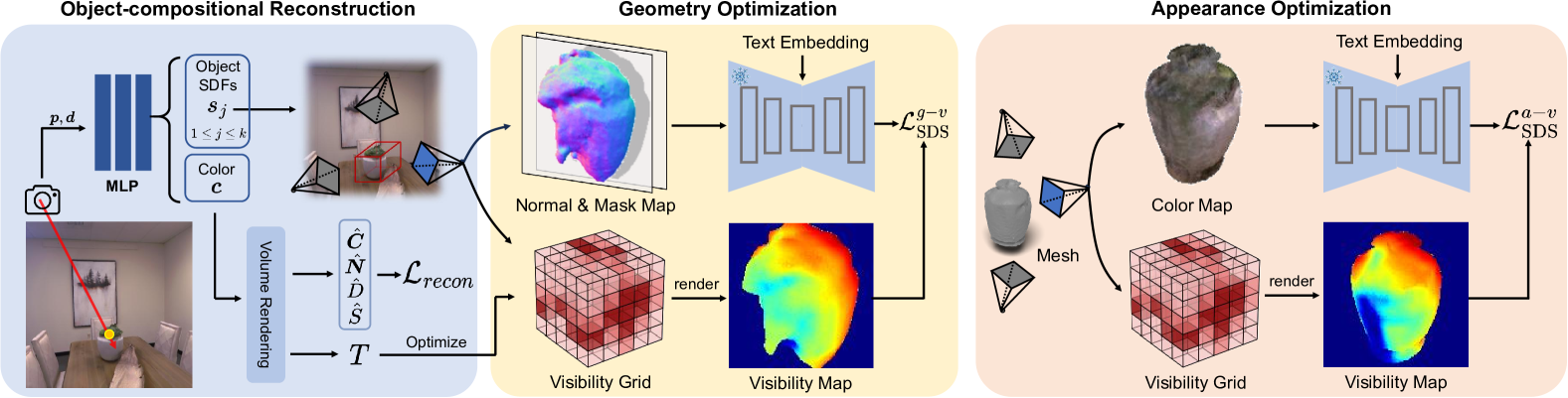
Figure 2: Overview of DP-Recon. We first use reconstruction loss $\mathcal{L}_{recon}$ for decompositional neural reconstruction, followed by the prior-guided geometry optimization stage that incorporates SDS loss $\mathcal{L}_{\text{SDS}}^{g-v}$. We finally export the object meshes and optimize their appearance with $\mathcal{L}_{\text{SDS}}^{a-v}$. The visibility balances the guidance from prior and reconstruction by dynamically adjusting per-pixel SDS loss.

2.3 Diffusion Prior for 3D Reconstruction

Recently, diffusion models have proven effective in providing prior knowledge for reconstruction [109, 45, 74, 6, 66, 51]. DreamFusion [65] introduces SDS with Stable Diffusion [69] to guide 3D object generation from text prompts. Methods such as ReconFusion [93], NeRFiller [89], MVIP-NeRF [5], and ExtraNeRF [75] refine fine-tuned 2D diffusion models to recover or inpaint high-fidelity NeRF from sparse input views. More recent approaches leverage video diffusion models [55, 18, 43, 46, 50] for improved consistency across views. However, these methods only focus on the novel view synthesis by applying diffusion priors to the entire scene, without awareness of individual objects. While the results seem reasonable, they fail to maintain the 3D consistency of objects across views, do not recover the 3D geometry of objects and cannot reconstruct regions behind occlusion. On the contrary, our method leverages the benefits of decompositional scene reconstruction and applies a generative prior to each object. This substantially enhances the reconstruction quality of both individual objects and the overall scene, in terms of both geometry and appearance. Moreover, we identify a critical issue overlooked in prior work: the conflict between generative and reconstruction guidance, and introduce a novel visibility-guided strategy to dynamically adjust the SDS loss during training, effectively resolving this conflict.

3 Method

Given a set of posed RGB images and corresponding instance masks, we aim to reconstruct the geometry and appearance of objects and the background in the scene. Fig.˜2 presents an overview of our proposed DP-Recon.

3.1 Background

SDF-based Neural Implicit Surfaces

NeRF [57] learns the density field $\sigma(\bm{p})$ and color field $\bm{c}(\bm{p},\bm{d})$ from input images for each point $\bm{p}$ and view direction $\bm{d}$. To reconstruct the 3D geometric surface, current approaches [85, 97] replace the NeRF density $\sigma(\bm{p})$ by a learnable transformation function of SDF value $s(\bm{p})$, which is defined as the signed distance from point $\bm{p}$ to the boundary surface. Following MonoSDF [103], for a ray $\bm{r}$ with view direction $\bm{d}$, we use the SDF $s(\bm{p}_{i})$ and the color $\bm{c}(\bm{p}_{i},\bm{d})$ for each point $\bm{p}_{i}$ along the ray to render the color $\hat{\bm{C}}(\bm{r})$ by volume rendering:

$$\hat{\bm{C}}(\bm{r})=\sum_{i=0}^{n-1}T_{i}\alpha_{i}\bm{c}_{i},$$ (1)

where $T_{i}$ is the discrete accumulated transmittance, and $\alpha_{i}$ is the discrete opacity value, defined as:

$$T_{i}=\prod_{j=0}^{i-1}(1-\alpha_{j}),\quad\alpha_{i}=1-exp(-\sigma_{i}\delta_{i}),$$ (2)

where $\delta_{i}$ represents the distance between neighboring sample points along the ray. Depth $\hat{D}(\bm{r})$ and normal $\hat{\bm{N}}(\bm{r})$ can also be derived through volume rendering.

Object-compositional Scene Reconstruction

Following previous work [91, 92, 42, 58], we consider the decompositional reconstruction of objects utilizing their corresponding masks and treat the background as an object. Specifically, for a scene with $k$ objects, we predict $k$ SDFs for each point $\bm{p}$ and the $j$-th $(1\leq j\leq k)$ SDF $s_{j}(\bm{p})$ is for the $j$-th object. The scene SDF $s(\bm{p})$ is the minimum of the object SDFs. We use the SDF $s_{j}(\bm{p})$ and the color $\bm{c}(\bm{p}_{i},\bm{d})$ to render color $\hat{\bm{C}}_{j}(\bm{r})$, depth $\hat{D}_{j}(\bm{r})$ and normal $\hat{\bm{N}}_{j}(\bm{r})$ for $j$-th object. See more details in the supplementary.

Score distillation sampling

DreamFusion [65] enables the optimization of any differentiable image generator, e.g. 3D NeRF, from textual descriptions by employing a pre-trained 2D diffusion model [70, 69]. Formally, let $x=g(\theta)$ represent an image rendered by a differentiable generator $g$ with parameter $\theta$, DreamFusion leverages a diffusion model $\phi$ to provide a score function $\hat{\epsilon}_{\phi}(x_{t};y,t)$, which predicts the sampled noise $\epsilon$ given the noisy image $x_{t}$, text-embedding $y$, and noise level $t$. This score function guides the direction of the gradient for updating the parameter $\theta$, and the gradient is calculated by Score Distillation Sampling (SDS):

$$\nabla_{\theta}\mathcal{L}_{\text{SDS}}(\phi,x)=\mathbb{E}_{t,\epsilon}\left[w(t)\left(\hat{\epsilon}_{\phi}(x_{t};y,t)-\epsilon\right)\frac{\partial x}{\partial\theta}\right],$$ (3)

where $w(t)$ is a weighting function.

3.2 3D Reconstruction with Generative Priors

The latent neural representation of the 3D scene is primarily optimized by the reconstruction loss $\mathcal{L}_{recon}$ derived from volume rendering, following prior work [91, 92, 42]. However, regions with sparse capture or heavy occlusions often lead to suboptimal geometry and appearance recovery due to insufficient information as reconstruction guidance. To mitigate this gap, we introduce diffusion prior to optimize the the 3D model, both in geometry and appearance, so that it looks realistic at novel unobserved views.

Prior-guided Geometry Optimization

We adopt the decompositional neural implicit surface as our 3D representation, which is parameterized with a series of multi-layer perceptrons with parameter $\theta$. The rendering functions in Sec.˜3.1 serve as the image generator $g(\theta)$. At each training iteration, we sample the $j$-th object and render its normal map and mask map at a randomly sampled camera pose. Following previous work [6, 66], we use a concatenated map $\tilde{n}_{j}$ of the normal and mask maps as the input for the diffusion model to improve geometric optimization stability. We then employ the SDS loss to compute the gradient for updating $\theta$ as follows:

$$\nabla_{\theta}\mathcal{L}_{\text{SDS}}^{g}=\mathbb{E}_{t,\epsilon}\left[w(t)\left(\hat{\epsilon}_{\phi}(z_{t};y,t)-\epsilon\right)\frac{\partial z}{\partial\tilde{n}_{j}}\frac{\partial\tilde{n}_{j}}{\partial\theta}\right],$$ (4)

where $z$ is the latent code of $\tilde{n}_{j}$. The background is also treated as one object for geometry optimization.

Prior-guided Appearance Optimization

To produce object meshes with detailed UV maps, which are friendly for photorealistic rendering in common 3D software and enable more downstream applications, we directly optimize the mesh appearance rather than NeRF’s appearance field. More specifically, we export the mesh for each object after the geometry optimization stage. Using NVDiffrast [37] for differentiable mesh rendering, we employ another small network $\psi$ to predict color for the mesh surface points. At each training iteration, the color map $c_{j}$ for $j$-th is rendered at a randomly selected camera view, and the appearance SDS loss is used to compute the gradient for updating $\psi$:

$$\nabla_{\psi}\mathcal{L}_{\text{SDS}}^{a}=\mathbb{E}_{t,\epsilon}\left[w(t)\left(\hat{\epsilon}_{\phi}(z_{t};y,t)-\epsilon\right)\frac{\partial z}{\partial c_{j}}\frac{\partial c_{j}}{\partial\psi}\right],$$ (5)

where $z$ is the latent code of $c_{j}$. Note that the color rendering loss from input views is also used to optimize $\psi$.

Background Appearance Optimization

Applying appearance SDS in Eq.˜5 for background optimization can lead to degenerated results, e.g., introducing non-existent objects, as the background lacks clear geometric cues from the local camera perspective. To mitigate this shape-appearance ambiguity, we use depth-guided inpainting [106] for the background panorama color map and employ the inpainted panorama to supervise background color during the appearance optimization stage. The inpainting mask is based on the visibility of the pixel in the panorama, derived from our visibility modeling introduced in Sec.˜3.3.

3.3 Visibility-guided Optimization

Score Distillation Sampling (SDS), despite its wide application, has been shown to suffer from significant artifacts [102, 38], such as oversaturation, oversmoothing, and low-diversity, and optimization instability [87, 54]. They become even more significant when optimizing the latent 3D representation through both reconstruction and SDS guidance, due to their potential conflict, leading to inconsistencies with the observations. We address this problem by proposing a visibility-guided approach, which adjusts geometry and appearance SDS loss based on pixel visibility in the input view when rendered from a novel view.

Visibility Modeling

We introduce a learnable visibility grid $G$ to model the visibility $v$ of a 3D point $\bm{p}$ in the input views. We employ a view-independent modeling for visibility, i.e., $v=G(\bm{p})$, as it only depends on the input views and is independent of the ray direction from novel views.

Table 1: Quantitative results on reconstruction and novel view synthesis. Our method achieves superior or comparable reconstruction and rendering quality compared to the baselines. This highlights the effectiveness of incorporating a generative prior to improve overall reconstruction quality, while the visibility modeling ensures stability in the observable parts, preventing drastic changes.

Dataset	Method	Reconstruction			Rendering
		CD$\downarrow$	F-Score $\uparrow$	NC$\uparrow$	PSNR$\uparrow$	SSIM$\uparrow$	LPIPS$\downarrow$	MUSIQ$\uparrow$
Replica	ZeroNVS*	21.53	16.41	79.43	14.47	0.515	0.428	45.78
	FreeNeRF	67.75	6.63	48.59	13.69	0.437	0.513	37.54
	MonoSDF	12.57	43.25	83.14	22.44	0.809	0.246	36.02
	RICO	17.36	27.89	82.27	19.85	0.746	0.356	31.82
	ObjectSDF++	8.57	50.11	85.44	24.66	0.865	0.198	41.42
	Oursgeo	7.91	50.99	89.36	25.08	0.868	0.196	43.33
	Ours	7.91	50.99	89.36	24.52	0.846	0.286	49.22
ScanNet++	ZeroNVS*	36.69	6.48	69.61	12.22	0.463	0.443	41.36
	FreeNeRF	134.34	1.50	46.46	15.32	0.533	0.481	35.42
	MonoSDF	18.52	26.72	76.26	17.58	0.646	0.451	28.63
	RICO	23.64	21.28	65.28	15.74	0.616	0.467	26.95
	ObjectSDF++	10.67	44.78	78.18	19.43	0.741	0.332	33.64
	Oursgeo	10.18	45.13	81.87	20.13	0.752	0.319	38.43
	Ours	10.18	45.13	81.87	20.17	0.715	0.442	45.71

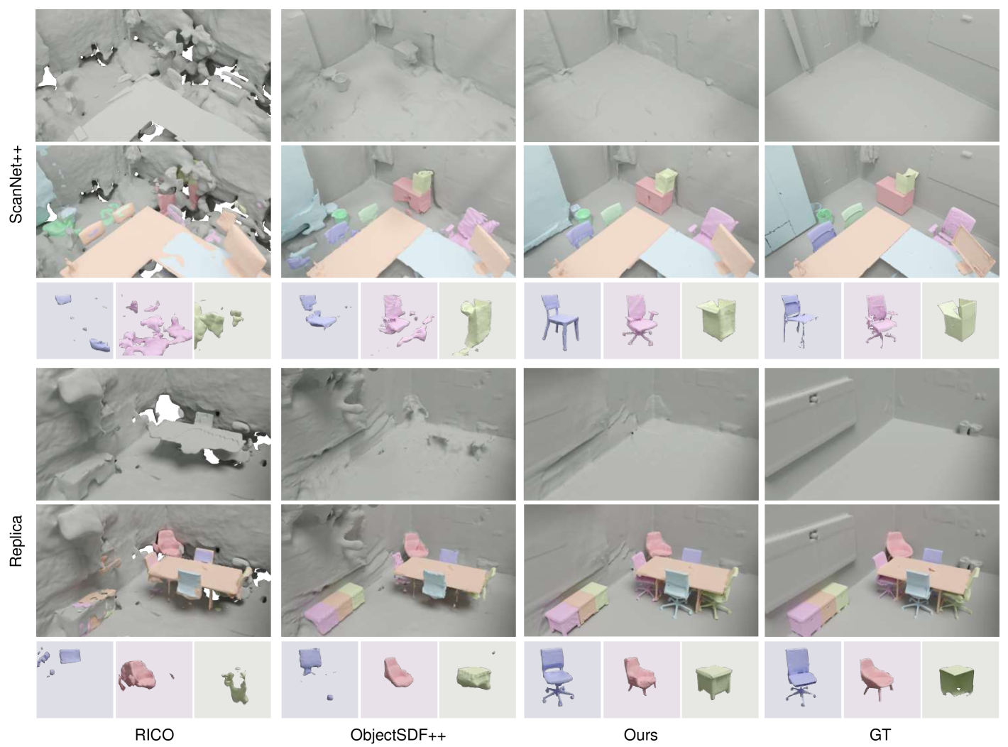
Figure 3: Qualitative comparison of 10-views reconstruction. We present examples from ScanNet++ [99] and Replica [80]. In each example, the first row shows the background, the second the full scene, and the third individual objects. We reconstruct more complete and reasonable 3D geometry, especially in less captured and occluded regions, such as the chair behind the table and the background.

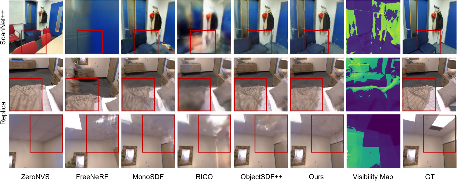
Figure 4: Qualitative results of novel view synthesis. Our method significantly improves rendering quality, particularly in less captured regions with low visibility, shown in darker colors in the visibility maps, such as the highlighted corner of the wall.

Ideally, points observed in more input views should have higher visibility. The accumulated transmittance $T$ for a 3D point $\bm{p}$ represents the probability that the corresponding ray reaches $\bm{p}$ without hitting any other particles - higher transmittance $T$ means greater visibility probability in the input views. Therefore, we initialize $G$ as zero and utilize the $T$ from input views to optimize the visibility grid $G$ via:

$$\mathcal{L}_{v}=\sum_{i=0}^{n}max(T_{i}-G(p_{i}),0).$$ (6)

We detach the gradient of $T_{i}$ to avoid the influence on the reconstruction network. We optimize $G$ after finishing the decompositional reconstruction stage to ensure the accuracy of the transmittance and freeze $G$ in the geometry and appearance optimization stage with generative diffusion prior.

Visibility-guided SDS

We obtain the visibility map $V$ under novel view by volume rendering similar to Eq.˜1. $V$ for a ray $r$ is calculated as $V(r)=\sum_{i=0}^{n-1}T_{i}\alpha_{i}v_{i}$. The visibility weighting function $w^{v}(z)$ is calculated as:

$$w^{v}(z)=\begin{cases}w_{0}+m_{0}V(z)&\text{if }V(z)\leq\tau\\ w_{1}+m_{1}V(z)&\text{if }V(z)>\tau\end{cases},$$ (7)

where $w$ and $m$ are piecewise linear coefficients, $V(z)$ denotes the pixel-wise visibility associated with latent $z$, and $\tau$ a threshold separating high and low visibility area. We reduce the SDS loss weight in high visibility regions to enhance reconstruction guidance while increasing SDS loss weight in low visibility regions for higher generative prior guidance. Then we rewrite Eq.˜4 and Eq.˜5 as:

$$\begin{split}\scalebox{0.95}{$\nabla_{\theta}\mathcal{L}_{\text{SDS}}^{g-v}=\mathbb{E}_{t,\epsilon}\left[w^{v}(z)w(t)\left(\hat{\epsilon}_{\phi}(z_{t};y,t)-\epsilon\right)\frac{\partial z}{\partial n_{j}}\frac{\partial n_{j}}{\partial\theta}\right]$}\\ \scalebox{0.95}{$\nabla_{\psi}\mathcal{L}_{\text{SDS}}^{a-v}=\mathbb{E}_{t,\epsilon}\left[w^{v}(z)w(t)\left(\hat{\epsilon}_{\phi}(z_{t};y,t)-\epsilon\right)\frac{\partial z}{\partial c_{j}}\frac{\partial c_{j}}{\partial\psi}\right]$}\end{split}$$ (8)

3.4 To Make Prior-Guided Optimization Work

Training process

Our training consists of three stages:

(1) Object-compositional reconstruction

The implicit surfaces are optimized to decompose the scene into individual objects with the reconstruction loss $\mathcal{L}_{recon}$ following prior work [92, 42]. See more details in supplementary. After this stage, we optimize the visibility grid $G$ by $\mathcal{L}_{v}$ in Eq.˜6 and keep it frozen in the following two stages.

(2) Geometry optimization

In addition to $\mathcal{L}_{recon}$, we also apply visibility-guided geometry SDS $\mathcal{L}_{\text{SDS}}^{g-v}$ for each object to optimize the latent representation.

(3) Appearance optimization

We export the mesh for each object after the geometry optimization and optimize the appearance network $\psi$ with $\mathcal{L}_{\text{SDS}}^{a-v}$ and color rendering loss. The appearance of the background is additionally reconstructed with the inpainted panorama.

Effective Rendering for SDS

As introduced above, $\mathcal{L}_{\text{SDS}}^{g-v}$ requires the normal and mask maps from volume rendering for iterative optimization. However, traditional volume rendering is slow, e.g., VolSDF [97] takes about 0.5 seconds to render a full image at $128\times 128$ resolution, which is impractical for optimization. To address this, we apply the OccGrid sampling method [40] to render normal map and mask map for SDS novel views, reducing rendering time to only 0.01 seconds for a $128\times 128$ resolution image.

Novel View Selection

SDS optimization requires novel view images rendered under object-centric camera poses. However, due to insufficient constraints with sparse views, NeRF-based methods produce floating artifacts throughout the scene, making it difficult to render object-centric images for each object. To address this, we use visibility grid $G$ to predict the boundary of each object and filter out the floaters. After filtering, we obtain the object’s bounding box and sample novel views for SDS around it. For the background, we randomly sample novel views within the scene.

Table 2: Decompositional object reconstruction. Our approach significantly outperforms baselines, recovering complete object meshes and smoother backgrounds with generative prior.

Method	Object Reconstruction				BG Reconstruction
	CD$\downarrow$	F-Score $\uparrow$	NC$\uparrow$	mIoU$\uparrow$	CD$\downarrow$	F-Score $\uparrow$	NC$\uparrow$
Replica
RICO	10.32	49.26	61.27	71.21	13.35	39.73	85.32
ObjectSDF++	7.49	56.69	64.75	71.72	10.33	44.19	86.34
Ours	5.54	67.71	73.50	88.21	9.39	46.14	92.83
ScanNet++
RICO	24.09	39.26	58.26	42.25	18.37	34.72	78.26
ObjectSDF++	14.52	46.87	61.57	45.73	13.20	38.92	80.47
Ours	5.03	66.55	72.91	70.01	11.51	40.12	86.24

4 Experiments

We evaluate DP-Recon on both geometry and appearance recovery for sparse-view 3D reconstruction. Additionally, we provide generalization results on YouTube videos, failure cases, and discuss limitations in supplementary.

4.1 Settings

Datasets

We conduct experiments on the synthetic dataset Replica [80] with 8 scenes following MonoSDF [103] and ObjectSDF++ [92]. Additionally, we use 6 scenes from the real-world dataset ScanNet++ [99]. We use 10 input views for each scene, except experiments on different input view numbers in Tab.˜3. See more details in supplementary.

Baselines

We compare against the state-of-tart sparse-view NeRF method FreeNeRF [95] and dense-view MonoSDF [103] with geometric regularization. We also compare with RICO [42] and ObjectSDF++ [92] for decompositional reconstruction. We adapt ZeroNVS [71], which synthesizes novel view of scenes from a single image, following ReconFusion [93] to multiview settings.

Table 3: Quantitative results on different view numbers. Our method outperforms baselines significantly under sparse-view settings.

	Scene Reconstruction (CD$\downarrow$ / NC$\uparrow$)			Object Reconstruction (CD$\downarrow$ / mIoU$\uparrow$)			Rendering (PSNR$\uparrow$/MUSIQ$\uparrow$)
Method	5 views	10 views	15 views	5 views	10 views	15 views	5 views	10 views	15 views
ZeroNVS*	31.86 / 75.26	21.53 / 79.43	20.80 / 81.81	-	-	-	13.72 / 39.01	14.47 / 45.78	15.02 / 46.39
FreeNeRF	76.83 / 48.19	67.76 / 48.59	65.26 / 49.71	-	-	-	12.94 / 27.71	13.69 / 37.54	13.89 / 37.13
MonoSDF	31.26 / 76.03	12.57 / 83.14	8.94 / 87.23	-	-	-	18.57 / 31.47	22.44 / 36.02	26.20 / 42.25
RICO	37.83 / 72.30	17.36 / 82.27	8.84 / 86.28	15.81 / 45.27	10.32 / 71.21	8.43 / 78.04	16.78 / 28.69	19.85 / 31.82	20.57 / 30.81
ObjectSDF++	35.49 / 68.86	8.57 / 85.44	7.21 / 88.21	9.35 / 47.63	7.49 / 71.72	6.93 / 80.01	17.43 / 28.13	24.66 / 41.42	27.33 / 44.36
Ours	12.63 / 83.72	7.91 / 89.36	6.78 / 91.79	6.66 / 69.48	5.54 / 88.21	4.88 / 87.39	20.43 / 39.28	24.52 / 49.22	28.12 / 50.71

Metrics

For reconstruction metrics, we evaluate Chamfer Distance (CD), F-Score, and Normal Consistency (NC) following MonoSDF [103] for both total scene and decompositional reconstruction. Additionally, we assess novel view mask Mean Intersection over Union (mIoU) to evaluate the completeness of object reconstruction. For rendering metrics, we evaluate full-reference (FR) and no-reference (NR) following ExtraNeRF [75]. For the FR metrics, we use PSNR, SSIM, and LPIPS and for NR, we employ MUSIQ [29] to evaluate the visual quality of rendered images. We randomly sample 10 novel views within each scene to evaluate the rendering metrics and mask mIoU.

4.2 Results

Table 4: Ablation study. Geometry (GP) and appearance (AP) priors improve the reconstruction and rendering quality, while the visibility (VG & VA) further enhances the consistency.

GP	VG	AP	VA	Scene Recon.		Rendering		Object Recon.		BG Recon.
				CD$\downarrow$	NC$\uparrow$	PSNR$\uparrow$	MUSIQ$\uparrow$	CD$\downarrow$	mIoU$\uparrow$	CD$\downarrow$	NC$\uparrow$
$\times$	$\times$	$\times$	$\times$	8.51	86.13	24.31	41.51	7.67	73.31	10.06	87.36
$\checkmark$	$\times$	$\times$	$\times$	8.14	88.68	24.83	41.98	6.35	84.45	9.83	91.36
$\checkmark$	$\checkmark$	$\times$	$\times$	7.91	89.36	25.08	43.33	5.54	88.21	9.39	92.83
$\checkmark$	$\times$	$\checkmark$	$\times$	8.14	88.68	22.83	50.25	6.35	84.45	9.83	91.36
$\checkmark$	$\checkmark$	$\checkmark$	$\times$	7.91	89.36	23.42	52.34	5.54	88.21	9.39	92.83
$\checkmark$	$\checkmark$	$\checkmark$	$\checkmark$	7.91	89.36	24.52	49.22	5.54	88.21	9.39	92.83

Holistic Scene Reconstruction

As shown in Tab.˜1, our method enhances both reconstruction and rendering results compared to all baselines. These improvements stem from incorporating generative priors into the reconstruction pipeline, which enables more accurate reconstruction in less captured areas, more precise object structures, smoother background reconstruction, and fewer floating artifacts, as illustrated in  Fig.˜3. Our appearance prior also supplies reasonable additional information in these less captured regions, allowing our NR rendering metric, MUSIQ, to significantly outperform the baselines. This indicates our rendering achieves higher quality in these areas, in contrast to the artifacts present in the baseline results, as shown in Fig.˜4.

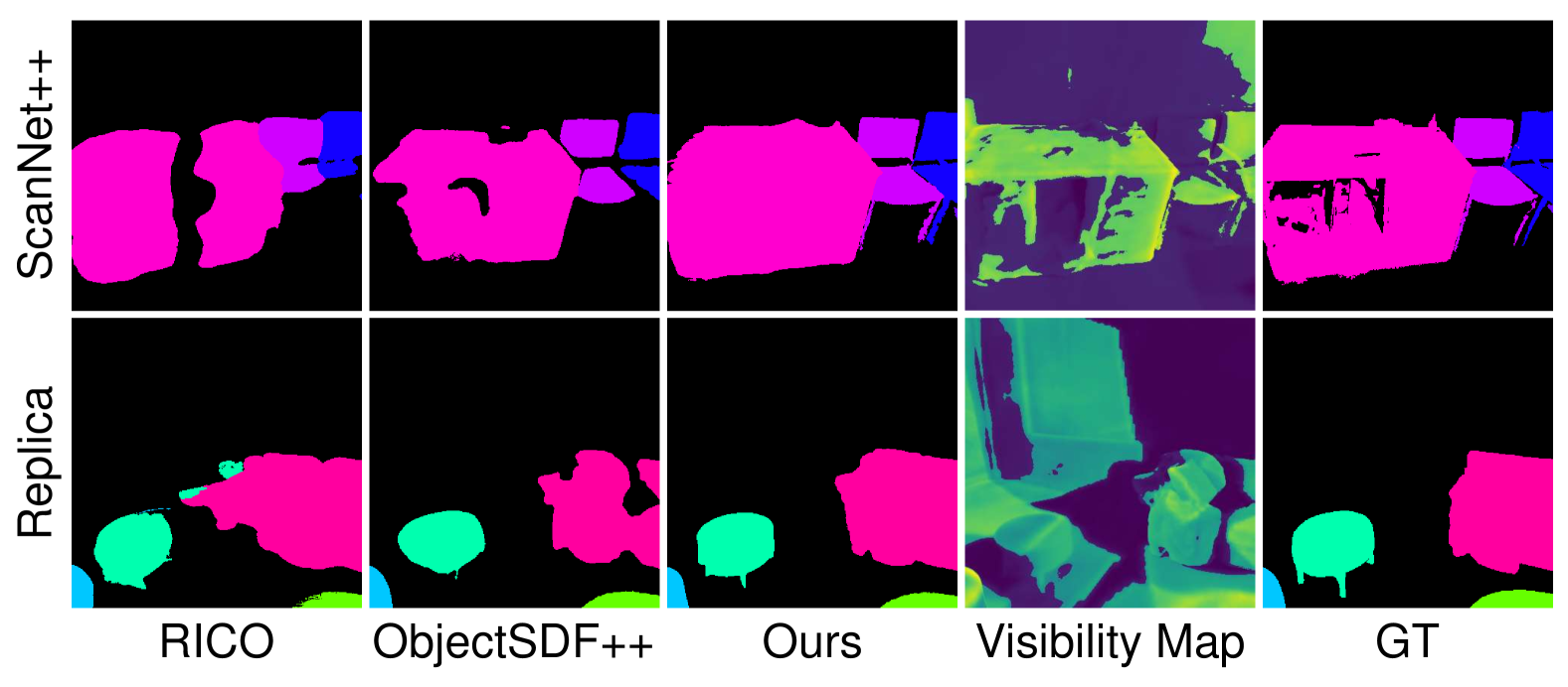
Figure 5: Visualized novel view instance masks. Our method can synthesize consistent and complete novel view instance masks.

Decompositional Object Reconstruction

Incorporating generative prior substantially improves the reconstruction in occluded regions, including more accurate object structures and fewer floating artifacts, e.g., the chair behind the table and the occluded background in Fig.˜3. The significant increase in novel view mask mIoU compared to all baselines shows that our method achieves complete and multi-view consistent object shapes, as illustrated in  Tab.˜2 and  Fig.˜5. Our results, shown in  Fig.˜3, remain faithful to input images in observed regions, confirming that our visibility-guided approach effectively mitigates conflicts between the guidance of generative prior and the input images.

Performance under Different View Number

Tab.˜3 shows our result consistently outperforms the baselines across varying numbers of input views, improving both geometry and appearance. Notably, it realizes better object reconstruction with just 5 views than baselines with 15 views. Our method is especially effective in large scenes with heavy occlusions, as demonstrated in Fig.˜1 where our method with 10 views outperforms the baseline with 100.

4.3 Ablation Studies

We design ablative studies on the geometry prior (GP), visibility guidance for geometry prior (VG), appearance prior (AP), and visibility guidance for appearance prior (VA). Tab.˜4 and Fig.˜6 reveal several key observations:

1. The integration of generative priors (GP & AP) substantially improves reconstruction and rendering quality. However, directly incorporating them creates inconsistencies with input views, potentially undermining the reconstruction of observed regions (see Fig.˜6 (b, e, f)).

2. As shown in Tab.˜4 and Fig.˜6 (c, g), visibility guidance (VG and VA) effectively regulates the influence of diffusion priors. By adaptively weighting the SDS loss, i.e., reducing its impact in high-visibility regions and amplifying it in low-visibility areas, our method achieves an optimal balance in prior-guided reconstruction.

3. The full model, incorporating all components, achieves the best overall performance. This demonstrates the effectiveness of our designs for geometry and appearance reconstruction, especially in unobserved regions.

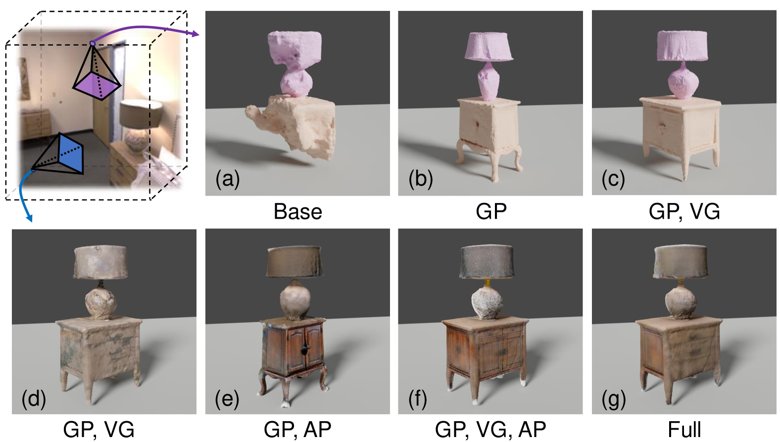
Figure 6: Qualitative ablation comparison. We show the meshes in the first row along with their textures in the second, demonstrating that prior knowledge can supplement missing information while the visibility modeling ensures consistency with input views.

4.4 Scene Editing

Text-based Editing

Leveraging decompositional reconstruction and text-guided generative priors, DP-Recon enables seamless text-based editing of both geometry (e.g., “A Teddy bear”) and appearance (e.g., “Space-themed”) for individual objects and background, as shown in Fig.˜7. This allows the generation of numerous digital replicas [80] or cousins [14] while preserving the original spatial layout.

VFX Editing

Our method reconstructs high-fidelity, decomposed object meshes with detailed UV maps, supporting VFX workflows in common 3D software like Blender. Fig.˜7 demonstrates diverse photorealistic VFX edits for individual objects (e.g., “Ignite it” or “Break it by a ball”), which could benefit filmmaking and game development.

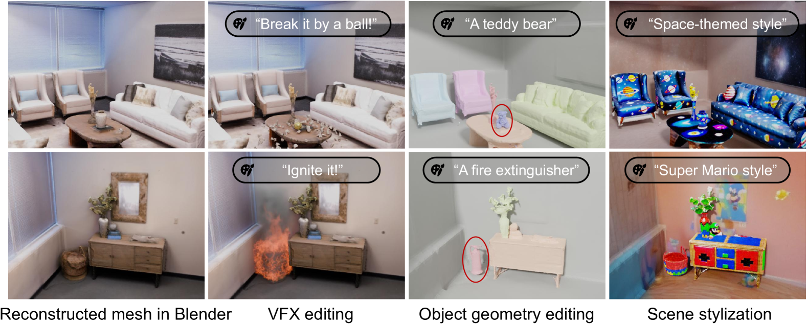
Figure 7: Examples of scene editing. Based on reconstructed scenes, our model seamlessly supports flexible text-guided geometry and appearance editing, as well as VFX editing.

5 Conclusion

We present DP-Recon, a novel pipeline that utilizes generative priors in the form of SDS to optimize the neural representation of each object. It employs a visibility-guided mechanism that dynamically adjusts the SDS loss, ensuring improved results while maintaining consistency with the input images. Extensive experiments demonstrate that our method outperforms state-of-the-art methods in both geometry and appearance reconstruction, effectively enhancing quality in unobserved regions while preserving fidelity in observed areas. Our method enables seamless text-based editing for geometry and stylization, and generates decomposed object meshes with detailed UV maps, supporting a wide range of downstream applications.

Supplementary Material

We provide details on the decompositional reconstruction process, training procedures, experimental setup, and a discussion of limitations. Additionally, we highly recommend watching the demo video on our webpage for a more intuitive and visually engaging presentation of the results.

Appendix A Generalizability to in-the-wild videos

Our method demonstrates robust generalizability to in-the-wild indoor scenes. Fig.˜S.8 presents reconstruction results of in-the-wild YouTube videos using 15 input views, with camera poses calibrated via COLMAP [72] and object masks obtained from SAM2 [67].

Appendix B Decompositional Reconstruction

We first present preliminary of decompositional scene reconstruction, also known as object-compositional reconstruction, which aims to reconstruct each object in the scene individually—including both foreground objects and the background—rather than representing the entire scene as a single, inseparable mesh.

Figure S.8: Generalizability to YouTube videos with 15 input views. The reconstruction results highlight our model’s robust ability to generalize to in-the-wild indoor scenes.

B.1 Decompositional Representation

Following previous work [91, 92, 42, 58], we utilize a set of posed RGB images and their corresponding instance masks to achieve decompositional reconstruction of objects, treating the background also as an object.

As described in the main paper, for a scene with $k$ objects, we predict $k$ SDFs for each point $\bm{p}$ and the $j$-th $(1\leq j\leq k)$ SDF $s_{j}(\bm{p})$ is for the $j$-th object. The scene SDF $s(\bm{p})$ is the minimum of the object SDFs:

$$s(\bm{p})=\min_{1\leq j\leq k}~s_{j}(\bm{p}),$$ (S.9)

The normal $\bm{n}(\bm{p})$ is the gradient of $s(\bm{p})$, while normal $\bm{n}^{j}(\bm{p})$ is the gradient of $s_{j}(\bm{p})$:

$$\bm{n}(\bm{p})=\nabla s(\bm{p}),\quad\bm{n}^{j}(\bm{p})=\nabla s_{j}(\bm{p})$$ (S.10)

Next, we transform each point’s SDFs into instance semantic logits $\bm{h}(\bm{p})=[h_{1}(\bm{p}),h_{2}(\bm{p}),\ldots,h_{k}(\bm{p})]$, where

$$h_{j}(\bm{p}) =\gamma/(1+\exp(\gamma\cdot s_{j}(\bm{p}))),$$ (S.11)

where $\gamma=10$ is a fixed parameter in our implementation.

B.2 Volume Rendering

For each camera ray $\bm{r}=(\bm{o},\bm{d})$ with $\bm{o}$ as the ray origin (camera center) and $\bm{d}$ as the viewing direction, $n$ points $\left\{\bm{p}_{i}=\bm{o}+t_{i}\bm{d}\mid i=0,1,\ldots,n-1\right\}$ are sampled, where $t_{i}$ is the distance from the sample point to the camera center. We predict $k$ SDFs and the color $\bm{c}_{i}$ for each point $\bm{p}_{i}$ along the ray. Then we compute scene SDF $s_{i}$, normal $\bm{n}_{i}$ and instance sematic logits $\bm{h}_{i}$ for point $\bm{p}_{i}$ by Eqs.˜S.9, S.10 and S.11. Next, we convert the scene SDF $s(\bm{p})$ into density $\sigma$ for volume rendering as in NeRF [57] following the method introduced in VolSDF [97]:

$$\sigma(s)=\begin{cases}\frac{1}{2\beta}\exp(\frac{s}{\beta})&s\leq 0\\ \frac{1}{\beta}(1-\exp(-\frac{s}{\beta}))&s\geq 0\end{cases},$$ (S.12)

where $\beta$ is a learnable parameter. We then calculate the discrete accumulated transmittance $T_{i}$ and discrete opacity $\alpha_{i}$ as follows:

$$T_{i}=\prod_{j=0}^{i-1}(1-\alpha_{j}),\quad\alpha_{i}=1-exp(-\sigma_{i}\delta_{i}),$$ (S.13)

where $\delta_{i}$ represents the distance between neighboring sample points along the ray.

Using volume rendering, the predicted scene color $\hat{\bm{C}}(\bm{r})$, depth $\hat{D}(\bm{r})$, normal $\hat{\bm{N}}(\bm{r})$ and instance semantic $\hat{\bm{S}}(\bm{r})$ for the ray $r$ are computed as:

$$\begin{split}\hat{\bm{C}}(\bm{r})&=\sum_{i=0}^{n-1}T_{i}\alpha_{i}\bm{c}_{i},\quad\hat{D}(\bm{r})=\sum_{i=0}^{n-1}T_{i}\alpha_{i}t_{i},\\ \hat{\bm{N}}(\bm{r})&=\sum_{i=0}^{n-1}T_{i}\alpha_{i}\bm{n}_{i},\quad\hat{\bm{S}}(\bm{r})=\sum_{i=0}^{n-1}T_{i}\alpha_{i}\bm{h}_{i},\end{split}$$ (S.14)

Additionally, replacing the scene SDF $s$ with $j$-th object SDF $s_{j}$ in Eqs.˜S.12 and S.13 allows rendering of the normal $\hat{\bm{N}}^{j}(\bm{r})$ and mask $\hat{O}^{j}(\bm{r})$ for $j$-th object as:

$$\hat{\bm{N}}^{j}(\bm{r})=\sum_{i=0}^{n-1}T^{j}_{i}\alpha^{j}_{i}\bm{n}^{j}_{i},\quad\hat{O}^{j}(\bm{r})=\sum_{i=0}^{n-1}T^{j}_{i}\alpha^{j}_{i},$$ (S.15)

B.3 Loss function

RGB Reconstruction Loss

Given input images, we employ RGB reconstruction loss $\mathcal{L}_{C}$ to minimize the difference between ground-truth pixel color and the rendered color. We follow the Yu et al. [103] here for the RGB reconstruction loss:

$$\mathcal{L}_{C}=\sum_{\bm{r}\in\mathcal{R}}||\hat{\bm{C}}(\bm{r})-\bm{C}(\bm{r})||_{1},$$ (S.16)

where $\hat{\bm{C}}(\bm{r})$ is the rendered color from volume rendering and $\bm{C}(\bm{r})$ denotes the ground truth.

Depth Consistency Loss

Monocular depth and normal cues [103] can greatly benefit indoor scene reconstruction. For the depth consistency, we minimize the difference between rendered depth $\hat{D}(\bm{r})$ and the depth estimation $\bar{D}(\bm{r})$ from the Depthfm model [21]:

$$\mathcal{L}_{D}=\sum_{\bm{r}\in\mathcal{R}}||(w\hat{D}(\bm{r})+q)-\bar{D}(\bm{r})||^{2},$$ (S.17)

where $w$ and $q$ are the scale and shift values to match the different scales. We solve $w$ and $q$ with a least-squares criterion, which has the closed-form solution. Please refer to the supplementary material of [103] for a detailed computation process.

Normal Consistency Loss

We utilize the normal cues $\bar{\bm{N}}(\bm{r})$ from Omnidata model [16] to supervise the rendered normal through the normal consistency loss, which comprises L1 and angular losses:

$$\mathcal{L}_{N}=\sum_{\bm{r}\in\mathcal{R}}||\hat{\bm{N}}(\bm{r})-\bm{\bar{N}}(\bm{r})||_{1}+||1-\hat{\bm{N}}(\bm{r})^{T}\bm{\bar{N}}(\bm{r})||_{1}.$$ (S.18)

The rendered normal $\hat{\bm{N}}(\bm{r})$ and normal cues $\bm{\bar{N}}(\bm{r})$ will be transformed into the same coordinate system by the camera pose.

Instance Semantic Loss

We minimize the semantic loss between rendered instance semantic logits of each pixel and the ground-truth pixel instance class. The instance semantic objective is implemented as a cross-entropy loss:

$$\mathcal{L}_{S}=\sum_{\bm{r}\in\mathcal{R}}\sum_{j=1}^{k}-\bar{h}_{j}(\bm{r})\log h_{j}(\bm{r}).$$ (S.19)

The $\bar{h}_{j}(\bm{r})$ is the ground-truth semantic probability for $j$-th object, which is $1$ or $0$.

Eikonal Loss and Smoothness Loss

Following common practice [97, 62], we add an Eikonal regularization and smoothness regularization term on the sampled points to regularize the SDF learning by:

$$\mathcal{L}_{eik}=\sum_{i=0}^{n-1}(||\nabla s(\bm{p}_{i})||_{2}-1),$$ (S.20)

$$\mathcal{L}_{smo}=\sum_{i=0}^{n-1}(||\nabla s(\bm{p}_{i})-\nabla s(\bm{\tilde{p}}_{i})||_{1}),$$ (S.21)

where $\bm{\tilde{p}}_{i}$ is randomly sampled nearby the $\bm{p}_{i}$.

Background Smoothness Loss

Following the previous work RICO [42], we use background smoothness loss to regularize the geometry of the occluded background to be smooth. Specifically, we randomly sample a $\mathcal{P}\times\mathcal{P}$ size patch every $\mathcal{T}_{\mathcal{P}}$ iterations within the given image and compute semantic map $\hat{\bm{H}}(\bm{r})$ and a patch mask $\hat{M}(\bm{r})$:

$$\hat{M}(\bm{r})=\mathds{1}[\arg\max(\hat{\bm{H}}(\bm{r}))\neq 1],$$ (S.22)

wherein the mask value is $1$ if the rendered class is not the background, thereby ensuring only the occluded background is regulated. Subsequently, we calculate the background depth map $\bar{D}(\bm{r})$ and background normal map $\bar{\bm{N}}(\bm{r})$ using the background SDF exclusively. The patch-based background smoothness loss is then computed as:

$$\begin{split}\mathcal{L}(\hat{D})&=\sum_{d=0}^{3}\sum_{m,n=0}^{\mathcal{P}-1-2^{d}}\hat{M}(\bm{r}_{m,n})\odot(|\hat{D}(\bm{r}_{m,n})-\\ &\hat{D}(\bm{r}_{m,n+2^{d}})|+|\hat{D}(\bm{r}_{m,n})-\hat{D}(\bm{r}_{m+2^{d},n})|),\end{split}$$ (S.23)

$$\begin{split}\mathcal{L}(\hat{\bm{N}})&=\sum_{d=0}^{3}\sum_{m,n=0}^{\mathcal{P}-1-2^{d}}\hat{M}(\bm{r}_{m,n})\odot(|\hat{\bm{N}}(\bm{r}_{m,n})-\\ &\hat{\bm{N}}(\bm{r}_{m,n+2^{d}})|+|\hat{\bm{N}}(\bm{r}_{m,n})-\hat{\bm{N}}(\bm{r}_{m+2^{d},n})|),\end{split}$$ (S.24)

$$\mathcal{L}_{bs}=\mathcal{L}(\hat{D})+\mathcal{L}(\hat{\bm{N}})$$ (S.25)

Object Distinction Regularization Loss

Following ObjectSDF++ [92], we employ a regularization term on object SDFs to penalize the overlap between any two objects:

$$\mathcal{L}_{sdf}=\sum_{i=0}^{n-1}(\sum_{j=1}^{k}ReLU(-s_{j}(\bm{p}_{i})-s(\bm{p}_{i}))).$$ (S.26)

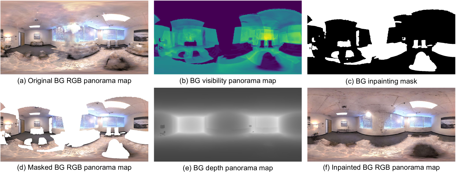
Figure S.9: Panorama inpainting of background. We present the original panorama map, the inpainted panorama map, the visibility panorama map, as well as the mask and depth guidance used in the depth-guided panorama inpainting process.

Appendix C More Training Details

C.1 Object-compositional Reconstruction

Overall Loss

We employ all the aforementioned losses in Sec.˜B.3 during the object-compositional reconstruction stage:

$$\begin{split}\mathcal{L}_{recon}&=\mathcal{L}_{C}+\lambda_{D}\mathcal{L}_{D}+\lambda_{N}\mathcal{L}_{N}+\lambda_{S}\mathcal{L}_{S}+\lambda_{bs}\mathcal{L}_{bs}\\ &+\lambda_{eik}\mathcal{L}_{eik}+\lambda_{smo}\mathcal{L}_{smo}+\lambda_{sdf}\mathcal{L}_{sdf},\end{split}$$ (S.27)

where the loss weights are set as $\lambda_{D}=0.1$, $\lambda_{N}=0.05$, $\lambda_{S}=1.0$, $\lambda_{bs}=0.1$, $\lambda_{eik}=0.1$, $\lambda_{smo}=0.005$, $\lambda_{sdf}=0.5$ following previous work [103, 42, 92].

Optimization of Visibility Grid

At the end of the object-compositional reconstruction stage, when the transmittance achieves sufficient accuracy, we optimize the visibility grid $G$. During this process, all input views are rendered $M$ times using  Eq.˜S.14, and the accumulated transmittance $T_{i}$ is utilized to optimize the visibility value of point $\bm{p}_{i}$. Note that $M$ is a hyperparameter that impacts the final visibility grid values; in our implementation, we set $M=20$. After the optimization, the visibility grid is frozen for the subsequent geometry and appearance optimization stages.

C.2 Geometry Optimization

Input for the Diffusion Model

In the common case, the encoder of Stable Diffusion [69] is used to encode an image into the latent code $z$ during SDS, followed by employing the UNet of Stable Diffusion to predict the score $\hat{\epsilon}$ and compute the SDS loss. However, the encoding process is relatively slow in computational speed. To address this issue and facilitate efficient training, following the previous work [6, 66], at each training iteration, we directly downsample the concatenated map $\tilde{n}_{j}$, which consists of the normal map $\hat{\bm{N}}^{j}(\bm{r})$ and mask map $\hat{O}^{j}(\bm{r})$ rendered by Eq.˜S.15 for sampled $j$-th object, into the latent code $z$ dimension. This approach reduces the computation time by approximately half without causing any performance degradation compared to directly inputting the normal map $\hat{\bm{N}}^{j}(\bm{r})$ into the encoder.

Overall Loss

We employ reconstruction loss $\mathcal{L}_{recon}$ in Eq.˜S.27 and visibility-guided geometry SDS loss $\mathcal{L}_{\text{SDS}}^{g-v}$ in the geometry optimization stage:

$$\mathcal{L}_{geo}=\mathcal{L}_{recon}+\lambda_{sds}^{geo}\mathcal{L}_{\text{SDS}}^{g-v},$$ (S.28)

where $\lambda_{sds}^{geo}=1e^{-5}$ in our implementation.

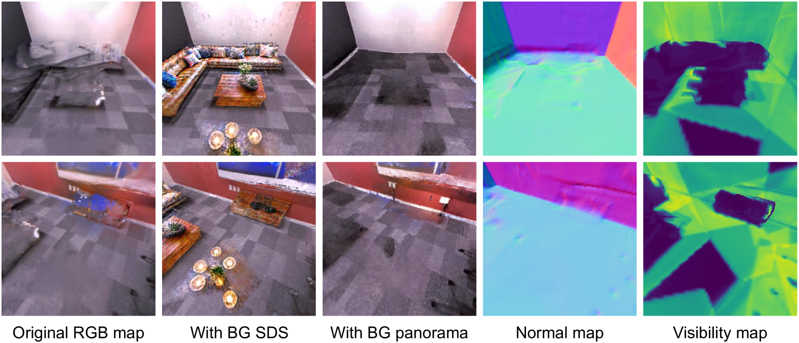
Figure S.10: Failure case of directly optimizing background with SDS loss. Incorporating appearance SDS for the background may result in hallucinated non-existent objects in low-visibility regions, even when the smooth normal map indicates no objects in the background. On the contrary, the background map obtained after optimizing depth-guided panorama inpainting produces a cleaner and more reasonable background texture.

C.3 Appearance Optimization

Rendering Loss in Appearance Optimization Stage

We employ two types of color rendering losses during the appearance optimization stage to ensure consistency between the observed regions and the input views. The first type derives directly from the input views, where we apply $\mathcal{L}_{C}$ as defined in Eq.˜S.16. The second type leverages useful appearance information distilled from the reconstruction network. For this, we randomly sample camera views within the scene, render RGB and visibility maps, and use regions with high visibility for appearance supervision. The sum of these two color rendering losses is denoted as $\mathcal{L}_{C}^{a}$.

Depth-guided Panorama Inpainting and Loss for BG

Applying appearance SDS $\mathcal{L}_{\text{SDS}}^{a-v}$ for background appearance optimization often leads to degenerated results, e.g. introducing non-existent objects as shown in Fig.˜S.10, due to the lack of clear geometric cues in the background from the local camera perspective. To address this issue, inspired by previous work [86, 77], we adopt depth-guided inpainting [106] to refine the low-visibility regions of the background panorama color map. Specifically, we first generate the original RGB, visibility, and depth panorama maps, as shown in Fig.˜S.9 (a, b, e). Next, we obtain the inpainting mask (Fig.˜S.9 (c)) for regions where the visibility map falls below a threshold $\tau$ (set to $\tau=0.2$ in our implementation). Finally, we apply depth-guided inpainting to produce the inpainted RGB panorama map (Fig.˜S.9 (f)).

To supervise the background appearance during the appearance optimization stage, we transform the inpainted RGB panorama map into a set of perspective images with corresponding camera poses. At each training iteration, we sample $B$ perspective images $\bm{C}_{B}$ along with their associated camera poses. For these poses, we render the background color maps $\hat{\bm{C}}_{B}$, and define the background panorama loss as:

$$\mathcal{L}_{\text{bg-pano}}=\frac{1}{B}\sum_{i=1}^{B}||\hat{\bm{C}}_{B}-\bm{C}_{B}||_{1},$$ (S.29)

Overall Loss

We employ color rendering loss $\mathcal{L}_{C}^{a}$, background panorama loss $\mathcal{L}_{\text{bg-pano}}$ in Eq.˜S.29 and visibility-guided appearance SDS loss $\mathcal{L}_{\text{SDS}}^{a-v}$ in the appearance optimization stage:

$$\mathcal{L}_{app}=\lambda_{C}^{a}\mathcal{L}_{C}^{a}+\lambda_{\text{bg-pano}}\mathcal{L}_{\text{bg-pano}}+\mathcal{L}_{\text{SDS}}^{a-v},$$ (S.30)

where $\lambda_{C}^{a}=\lambda_{\text{bg-pano}}=1e^{4}$ in our implementation.

Export UV Map

Following previous works [6, 66], we utilize the trained $\psi$ to export the appearance of object mesh as UV map by the xatlas [101]. Our object mesh with exported UV map supports direct use and editing in common 3D software, e.g. Blender [11], as shown in Fig.˜S.11. We export $1024\times 1024$ UV map for foreground objects and $2048\times 2048$ UV map for the background in our case.

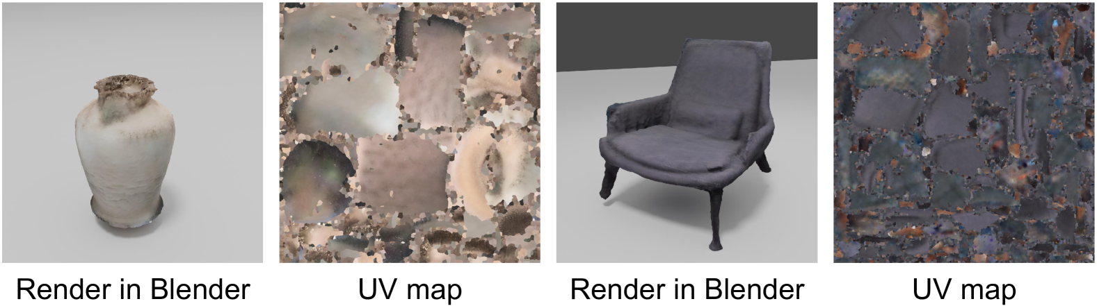
Figure S.11: Visualization of UV mapping and rendering results. Our method produces completed meshes with detailed UV maps, enabling photorealistic rendering in common 3D software such as Blender.

Appendix D More Experiment Details

D.1 Baselines Details

For MonoSDF [103], RICO [42], and ObjectSDF++ [92], which are designed for reconstruction, we directly utilize the official code to obtain the reconstructed meshes and rendered images. For FreeNeRF [95], which focuses on novel view synthesis and does not include reconstruction code, we first predict depth maps and RGB images for densely sampled camera views within the scene. We then apply TSDF Fusion [13] to integrate the predicted depth maps into a TSDF volume and export the resulting mesh. ZeroNVS [71] trains a diffusion model to synthesize novel views of scenes from a single image. To adapt it for multi-view inputs, we follow the approach of ReconFusion [93], using the input view closest to the novel view as the conditioning view for the diffusion model. We denote the adapted version as ZeroNVS*. Subsequently, we use MonoSDF to reconstruct the scene mesh from the images synthesized by ZeroNVS*.

D.2 Data Preparation

Monocular Cues

We utilize the pre-trained DepthFM model [21] and Omnidata model [16] to generate the depth map $\bar{D}$ and normal map $\bar{\bm{N}}$ for each RGB image, respectively. While depth cues provide semi-local relative information, normal cues are inherently local, capturing fine geometric details. As a result, we expect surface normals and depth to complement each other effectively. It is worth noting that estimating absolute scale in general scenes remains challenging; therefore, $\bar{D}$ should be interpreted as a relative depth cue.

GT Instance Mask

For the ScanNet++ [99] dataset, we use the official rendering engine to generate instance masks for each image based on the provided GT mesh and per-vertex 3D instance annotations. For the Relica [80] datasets, we utilize the original instance masks from vMAP [34], which are overly fragmented, and manually merge adjacent fragmented instance masks into coherent objects. Furthermore, since both ScanNet++ and Replica only provide a complete mesh of the scene, we derive the background GT mesh by removing the object meshes from the total mesh and manually filling the holes.

Notably, with the rapid advancement of segmentation and tracking models, such as SAM [33] and SAM2 [67], it’s more feasible to extract object masks directly from images using off-the-shelf models. These tools could inspire further progress in decompositional neural scene reconstruction.

D.3 Reconstruction Metrics Details

Following previous research [103, 42, 92], we evaluate the CD in $cm$, F-score with a threshold of $5cm$ and NC for 3D scene and object reconstruction. Consistent with previous studies [103, 42, 92], reconstruction is evaluated only on visible areas for the entire scene, while complete meshes are assessed for individual objects and background meshes. These metrics are defined in Tab.˜S.5.

Since the baselines ZeroNVS* [71], FreeNeRF [95] and MonoSDF [103] can only reconstruct the total scene and cannot decompose it into individual objects, we evaluate the metrics only for the total scene, i.e., the total scene reconstruction metrics and rendering metrics.

Table S.5: Evaluation metrics. We show the evaluation metrics with their definitions that we use to measure reconstruction quality. $P$ and $P^{*}$ are the point clouds sampled from the predicted and the ground truth mesh. $\bm{n}_{\bm{p}}$ is the normal vector at point $\bm{p}$.

Metric	Definition
Chamfer Distance (CD)	$\frac{\textit{Accuracy}+\text{Completeness}}{2}$
Accuracy	$\underset{\bm{p}\in P}{\mbox{mean}}\left(\underset{\bm{p}^{*}\in P^{*}}{\mbox{min}}||\bm{p}-\bm{p}^{*}||_{1}\right)$
Completeness	$\underset{\bm{p}^{*}\in P^{*}}{\mbox{mean}}\left(\underset{\bm{p}\in P}{\mbox{min}}||\bm{p}-\bm{p}^{*}||_{1}\right)$
F-score	$\frac{2\times\text{Precision}\times\text{Recall}}{\text{Precision}+\text{Recall}}$
Precision	$\underset{\bm{p}\in P}{\mbox{mean}}\left(\underset{\bm{p}^{*}\in P^{*}}{\mbox{min}}||\bm{p}-\bm{p}^{*}||_{1}<0.05\right)$
Recall	$\underset{\bm{p}^{*}\in P^{*}}{\mbox{mean}}\left(\underset{\bm{p}\in P}{\mbox{min}}||\bm{p}-\bm{p}^{*}||_{1}<0.05\right)$
Normal Consistency	$\frac{\textit{Normal Accuracy}+\textit{Normal Completeness}}{2}$
Normal Accuracy	$\underset{\bm{p}\in P}{\mbox{mean}}\left(\bm{n}_{\bm{p}}^{T}\bm{n}_{\bm{p}^{*}}\right)\,\,\text{s.t.}\,\,\bm{p}^{*}=\underset{\bm{p}^{*}\in P^{*}}{arg\,min}||\bm{p}-\bm{p}^{*}||_{1}$
Normal Completeness	$\underset{\bm{p}^{*}\in P^{*}}{\mbox{mean}}\left(\bm{n}_{\bm{p}}^{T}\bm{n}_{\bm{p}^{*}}\right)\,\,\text{s.t.}\,\,\bm{p}=\underset{\bm{p}\in P}{arg\,min}||\bm{p}-\bm{p}^{*}||_{1}$

Table S.6: Training time and performance comparison. Our method outperforms baselines in 4.5 hours per scene with 50,000 iterations.

Total Iter	RICO			ObjectSDF++			Ours
	Time	CD$\downarrow$	F-Score$\uparrow$	Time	CD$\downarrow$	F-Score$\uparrow$	Time	CD$\downarrow$	F-Score$\uparrow$
40000	2.63h	21.30	49.47	2.34h	18.48	52.51	2.59h	12.96	61.87
50000	3.16h	17.37	52.33	2.93h	13.36	60.37	4.52h	4.51	72.66
60000	3.82h	14.63	57.74	3.42h	5.42	70.19	6.54h	4.35	73.23
80000	5.01h	12.09	63.39	4.48h	5.10	70.87	10.45h	4.33	73.32

D.4 Implementation Details

We implement our model in PyTorch [64] and utilize the Adam optimizer [32] with an initial learning rate of $5e-4$. In the object-compositional reconstruction stage, we sample 1024 rays per iteration, and in the geometry and appearance optimization stages, we render $128\times 128$ images for normal, mask, and color maps. We use $2048\times 1024$ for the background panorama map.

For visibility guided SDS:

$$w^{v}(z)=\begin{cases}w_{0}+m_{0}V(z)&\text{if }V(z)\leq\tau\\ w_{1}+m_{1}V(z)&\text{if }V(z)>\tau\end{cases},$$ (S.31)

we set $\tau=0.5,w_{0}=20,m_{0}=-38,w_{1}=2,m_{1}=-2$ for the geometry optimization stage. Under this configuration, $w^{v}(z)$ achieves a maximum value of $20$ when $V(z)=0$, a minimum value of $0$ when $V(z)=1$, and a value of $1$ when $V(z)=\tau=0.5$. For appearance optimization stage, we set $\tau=0.3,w_{0}=1,m_{0}=0,w_{1}=0,m_{1}=0$, which results in $w^{v}(z)=1$ when $V(z)\leq 0.3$ and $w^{v}(z)=0$ when $V(z)>0.3$.

Our model is trained for 80000 iterations on both Replica [80] and ScanNet++ [99] datasets. The geometry optimization stage and appearance optimization stage begin at the $35000^{th}$ and $75000^{th}$ iterations, respectively. All experiments are conducted on a single NVIDIA-A100 GPU, requiring approximately 10 hours to complete the training of a single scene.

D.5 Training Time Comparison

For a fair comparison with prior work [103, 92, 42], we train our model and all baselines for 80,000 iterations in all main paper experiments. Detailed training time and performance results are provided in Tab.˜S.6, showing that our method outperforms baselines in approximately 4.5 hours per scene with 50,000 iterations.

Appendix E Scene Editing Details

E.1 Text-based Editing

With our decompositional representation, which breaks down each object’s representation in the scene, we can seamlessly edit the representation of any object in the scene based on the text prompt, with the generative capabilities of our SDS diffusion prior. With the two forms of SDS prior we introduced, i.e., the geometry SDS prior and the appearance SDS prior, we can freely edit both the geometry and appearance of objects. During the editing process, we exclude the reconstruction loss for the edited object and disable the visibility guidance.

Geometry Editing

We realize geometry editing for objects in the geometry optimization stage using geometry SDS loss $\mathcal{L}_{\text{SDS}}^{g}$. During optimization, we replace the original object prompt with the desired object prompt while continuing to sample novel camera views around the original object’s bounding box. This ensures that the desired object retains the same location as the original one.

Appearance Editing

We perform object appearance editing during the appearance optimization stage using the appearance SDS loss $\mathcal{L}_{\text{SDS}}^{a}$. For this task, we not only modify the object prompt but also update the negative prompt in Stable Diffusion [69], as suggested in the prompt engineering tutorial [2]. Empirically, we observe that appearance optimization is more sensitive to the choice of the negative prompt compared to geometry optimization. For scene stylization, we use a consistent style prompt for editing the appearance of not only all objects but also generating the background panorama, which is achieved through depth-guided ControlNet [106].

E.2 VFX Editing

The object meshes reconstructed by our method feature detailed UV maps, making them compatible with common 3D software and enabling diverse and photorealistic VFX editing. We implement our VFX editing in Blender, as demonstrated in our main paper. More specifically,

• “Freeze it” utilizes the Geometry Nodes Modifier and applies a glass material over the original object.

• “Ignite it” employs the Quick Smoke Effect, setting the Flow Type to Fire and Smoke, with fire color adjustments via Shading Nodes.

• “Break it by a ball” uses the Cell Fracture Effect to divide the object into multiple fragments, assigning both the object and ball as Rigid Bodies for physics-based simulation in Blender.

Appendix F Comparison with Image-to-3D Method

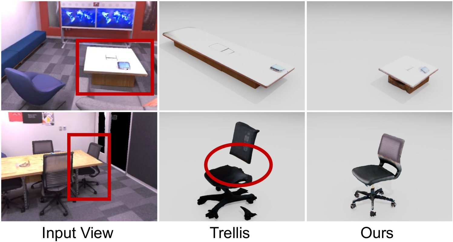
Figure S.12: Comparison with image-to-3D method Trellis [94]. For better visualization, we adjust the location and rotation of Trellis results manually.

Unlike decompositional scene reconstruction methods, which recover object geometry along with location, rotation, and scale simultaneously from multi-view images, an alternative approach is to use image-to-3D models for extracting individual objects within a scene. However, as shown in Fig.˜S.12, these models (e.g., Trellis [94]) face significant challenges in recovering the location, rotation, and scale of objects, with severe performance deterioration under occlusion, making them less applicable for scene reconstruction regardless of views compared to our method.

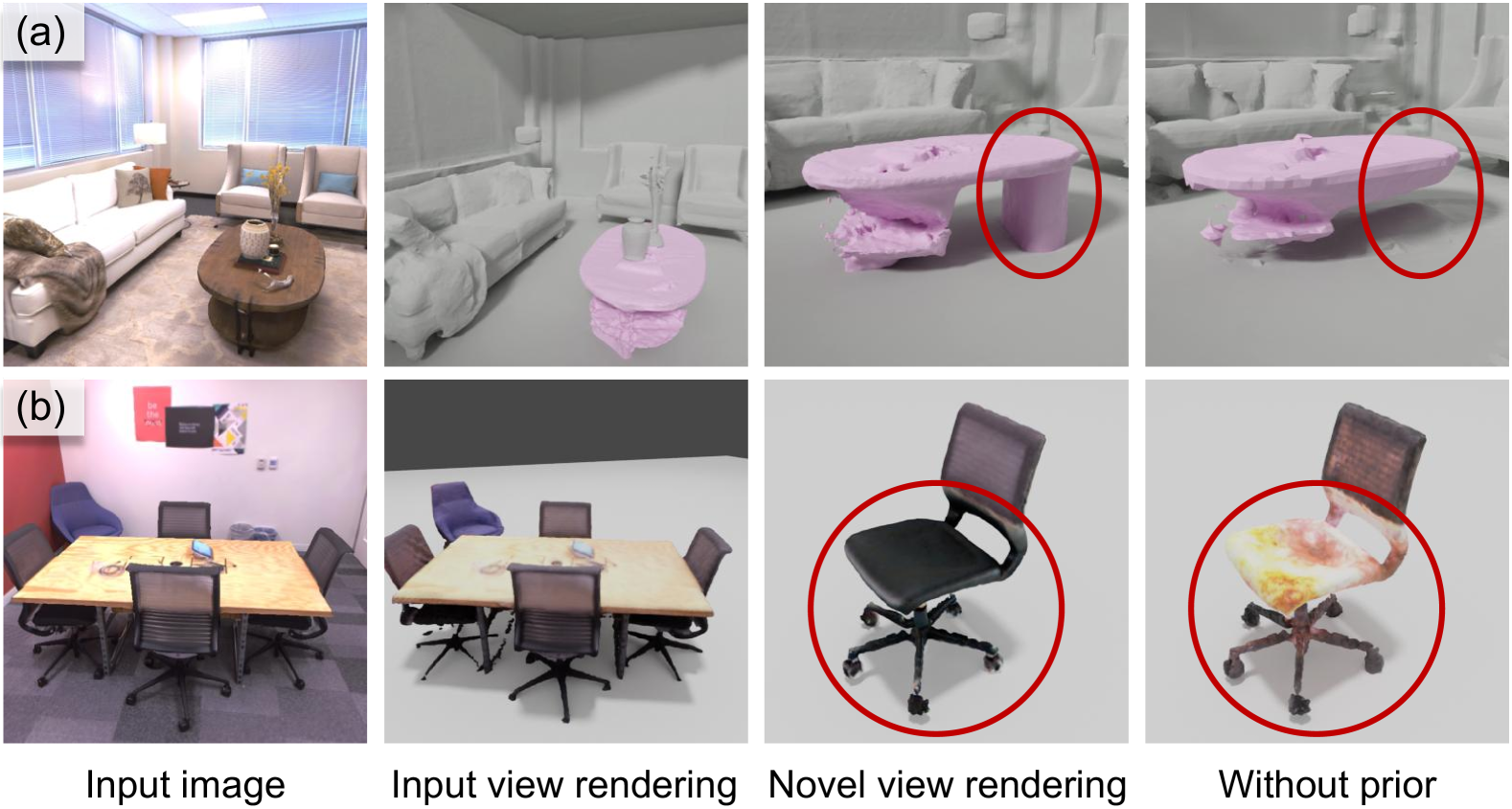
Figure S.13: Qualitative Examples for Failure Cases. We present failure cases for both geometry optimization and appearance optimization. The first column displays the input view, while the second and third columns show our results rendered from the input view and a novel view, respectively. The final column provides the corresponding results without applying the geometry prior (top) or appearance prior (bottom), highlighting the improvements introduced by our generative prior.

Appendix G Failure Cases and Limitation

In this section, we present and analyze examples of representative failure. Fig.˜S.13 (a) demonstrates that our method may produce non-harmonious structures with inaccurate text prompts. For instance, in this example, we use the prompt “A tea table”, but the table in this case does not conform to the conventional concept of a tea table. A similar issue arises during appearance optimization, as shown in Fig.˜S.13 (b), where we use the prompt “A black ergonomic chair”, but the chair in this case is not entirely black—it appears somewhat gray—resulting in a non-harmonious appearance in the completed regions. We believe that leveraging implicit prompts [17] could help alleviate such issues related to text prompts.

Moreover, our method optimizes each object independently in each iteration, using the 3D location information from the reconstruction module alone. This could be further improved by forming functional object groups by composing neighboring objects. Within these groups, SDS can be employed to optimize inter-object relationships and plausible layouts [108, 9]. Additionally, SDS-based methods [6, 66] struggle to reconstruct loose geometries such as grass, hair, sky, and fur, which are challenging to describe with text prompts. In contrast, concurrent methods [93, 18, 43, 46] that directly generate novel view images from sparse input views without relying on text prompts may mitigate this limitation. However, these methods often fail to maintain the 3D consistency of objects across views, achieve object-level editing, or reconstruct regions obscured by occlusions.

References

- Anderson et al. [2018] Peter Anderson, Qi Wu, Damien Teney, Jake Bruce, Mark Johnson, Niko Sünderhauf, Ian Reid, Stephen Gould, and Anton Van Den Hengel. Vision-and-language navigation: Interpreting visually-grounded navigation instructions in real environments. In Conference on Computer Vision and Pattern Recognition (CVPR), 2018.
- Andrew [2023] Andrew. Sdxl-styles. https://stable-diffusion-art.com/sdxl-styles/, 2023.
- Barron et al. [2022] Jonathan T Barron, Ben Mildenhall, Dor Verbin, Pratul P Srinivasan, and Peter Hedman. Mip-nerf 360: Unbounded anti-aliased neural radiance fields. In Conference on Computer Vision and Pattern Recognition (CVPR), 2022.
- Barron et al. [2023] Jonathan T Barron, Ben Mildenhall, Dor Verbin, Pratul P Srinivasan, and Peter Hedman. Zip-nerf: Anti-aliased grid-based neural radiance fields. In International Conference on Computer Vision (ICCV), pages 19697–19705, 2023.
- Chen et al. [2024a] Honghua Chen, Chen Change Loy, and Xingang Pan. Mvip-nerf: Multi-view 3d inpainting on nerf scenes via diffusion prior. In Conference on Computer Vision and Pattern Recognition (CVPR), 2024a.
- Chen et al. [2023] Rui Chen, Yongwei Chen, Ningxin Jiao, and Kui Jia. Fantasia3d: Disentangling geometry and appearance for high-quality text-to-3d content creation. In International Conference on Computer Vision (ICCV), 2023.
- Chen et al. [2024b] Yiwen Chen, Zilong Chen, Chi Zhang, Feng Wang, Xiaofeng Yang, Yikai Wang, Zhongang Cai, Lei Yang, Huaping Liu, and Guosheng Lin. Gaussianeditor: Swift and controllable 3d editing with gaussian splatting. In Conference on Computer Vision and Pattern Recognition (CVPR), 2024b.
- Chen et al. [2024c] Yixin Chen, Junfeng Ni, Nan Jiang, Yaowei Zhang, Yixin Zhu, and Siyuan Huang. Single-view 3d scene reconstruction with high-fidelity shape and texture. In International Conference on 3D Vision (3DV), 2024c.
- Chen et al. [2024d] Yongwei Chen, Tengfei Wang, Tong Wu, Xingang Pan, Kui Jia, and Ziwei Liu. Comboverse: Compositional 3d assets creation using spatially-aware diffusion guidance. In European Conference on Computer Vision (ECCV), 2024d.
- Chibane et al. [2020] Julian Chibane, Thiemo Alldieck, and Gerard Pons-Moll. Implicit functions in feature space for 3d shape reconstruction and completion. In Conference on Computer Vision and Pattern Recognition (CVPR), 2020.
- Community [2018] Blender Online Community. Blender - a 3d modelling and rendering package. Blender Foundation, Stichting Blender Foundation, Amsterdam, 2018.
- Cui et al. [2023] Jieming Cui, Ziren Gong, Baoxiong Jia, Siyuan Huang, Zilong Zheng, Jianzhu Ma, and Yixin Zhu. Probio: A protocol-guided multimodal dataset for molecular biology lab. In Advances in Neural Information Processing Systems (NeurIPS), 2023.
- Curless and Levoy [1996] Brian Curless and Marc Levoy. A volumetric method for building complex models from range images. In ACM SIGGRAPH / Eurographics Symposium on Computer Animation (SCA), 1996.
- Dai et al. [2024] Tianyuan Dai, Josiah Wong, Yunfan Jiang, Chen Wang, Cem Gokmen, Ruohan Zhang, Jiajun Wu, and Li Fei-Fei. Acdc: Automated creation of digital cousins for robust policy learning. arXiv preprint arXiv:2410.07408, 2024.
- Deng et al. [2022] Kangle Deng, Andrew Liu, Jun-Yan Zhu, and Deva Ramanan. Depth-supervised NeRF: Fewer views and faster training for free. In Conference on Computer Vision and Pattern Recognition (CVPR), 2022.
- Eftekhar et al. [2021] Ainaz Eftekhar, Alexander Sax, Jitendra Malik, and Amir Zamir. Omnidata: A scalable pipeline for making multi-task mid-level vision datasets from 3d scans. In International Conference on Computer Vision (ICCV), 2021.
- Gal et al. [2022] Rinon Gal, Yuval Alaluf, Yuval Atzmon, Or Patashnik, Amit H. Bermano, Gal Chechik, and Daniel Cohen-Or. An image is worth one word: Personalizing text-to-image generation using textual inversion. arXiv preprint arXiv:2208.01618, 2022.
- Gao* et al. [2024] Ruiqi Gao*, Aleksander Holynski*, Philipp Henzler, Arthur Brussee, Ricardo Martin-Brualla, Pratul P. Srinivasan, Jonathan T. Barron, and Ben Poole*. Cat3d: Create anything in 3d with multi-view diffusion models. In Advances in Neural Information Processing Systems (NeurIPS), 2024.
- Gong et al. [2023] Ran Gong, Jiangyong Huang, Yizhou Zhao, Haoran Geng, Xiaofeng Gao, Qingyang Wu, Wensi Ai, Ziheng Zhou, Demetri Terzopoulos, Song-Chun Zhu, et al. Arnold: A benchmark for language-grounded task learning with continuous states in realistic 3d scenes. arXiv preprint arXiv:2304.04321, 2023.
- Gu et al. [2023] Jiayuan Gu, Fanbo Xiang, Xuanlin Li, Zhan Ling, Xiqiang Liu, Tongzhou Mu, Yihe Tang, Stone Tao, Xinyue Wei, Yunchao Yao, et al. Maniskill2: A unified benchmark for generalizable manipulation skills. arXiv preprint arXiv:2302.04659, 2023.
- Gui et al. [2025] Ming Gui, Johannes S. Fischer, Ulrich Prestel, Pingchuan Ma, Dmytro Kotovenko, Olga Grebenkova, Stefan Andreas Baumann, Vincent Tao Hu, and Björn Ommer. Depthfm: Fast monocular depth estimation with flow matching. In AAAI Conference on Artificial Intelligence (AAAI), 2025.
- Hu et al. [2023] Shoukang Hu, Kaichen Zhou, Kaiyu Li, Longhui Yu, Lanqing Hong, Tianyang Hu, Zhenguo Li, Gim Hee Lee, and Ziwei Liu. Consistentnerf: Enhancing neural radiance fields with 3d consistency for sparse view synthesis. arXiv preprint arXiv:2305.11031, 2023.
- Huang et al. [2024] Jiangyong Huang, Silong Yong, Xiaojian Ma, Xiongkun Linghu, Puhao Li, Yan Wang, Qing Li, Song-Chun Zhu, Baoxiong Jia, and Siyuan Huang. An embodied generalist agent in 3d world. In International Conference on Machine Learning (ICML), 2024.
- Huang et al. [2025] Jiangyong Huang, Baoxiong Jia, Yan Wang, Ziyu Zhu, Xiongkun Linghu, Qing Li, Song-Chun Zhu, and Siyuan Huang. Unveiling the mist over 3d vision-language understanding: Object-centric evaluation with chain-of-analysis. In Conference on Computer Vision and Pattern Recognition (CVPR), 2025.
- Jain et al. [2021] Ajay Jain, Matthew Tancik, and Pieter Abbeel. Putting nerf on a diet: Semantically consistent few-shot view synthesis. In International Conference on Computer Vision (ICCV), 2021.
- Jiang et al. [2024a] Nan Jiang, Zimo He, Zi Wang, Hongjie Li, Yixin Chen, Siyuan Huang, and Yixin Zhu. Autonomous character-scene interaction synthesis from text instruction. In SIGGRAPH Asia 2024 Conference Papers, 2024a.
- Jiang et al. [2024b] Nan Jiang, Zhiyuan Zhang, Hongjie Li, Xiaoxuan Ma, Zan Wang, Yixin Chen, Tengyu Liu, Yixin Zhu, and Siyuan Huang. Scaling up dynamic human-scene interaction modeling. In Conference on Computer Vision and Pattern Recognition (CVPR), 2024b.
- Jiang et al. [2022] Yunfan Jiang, Agrim Gupta, Zichen Zhang, Guanzhi Wang, Yongqiang Dou, Yanjun Chen, Li Fei-Fei, Anima Anandkumar, Yuke Zhu, and Linxi Fan. Vima: General robot manipulation with multimodal prompts. arXiv preprint arXiv:2210.03094, 2022.
- Ke et al. [2021] Junjie Ke, Qifei Wang, Yilin Wang, Peyman Milanfar, and Feng Yang. Musiq: Multi-scale image quality transformer. In International Conference on Computer Vision (ICCV), 2021.
- Kerbl et al. [2023] Bernhard Kerbl, Georgios Kopanas, Thomas Leimkühler, and George Drettakis. 3d gaussian splatting for real-time radiance field rendering. In ACM SIGGRAPH / Eurographics Symposium on Computer Animation (SCA), 2023.
- Kim et al. [2022] Mijeong Kim, Seonguk Seo, and Bohyung Han. Infonerf: Ray entropy minimization for few-shot neural volume rendering. In Conference on Computer Vision and Pattern Recognition (CVPR), 2022.
- Kingma and Ba [2014] Diederik P Kingma and Jimmy Ba. Adam: A method for stochastic optimization. arXiv preprint arXiv:1412.6980, 2014.
- Kirillov et al. [2023] Alexander Kirillov, Eric Mintun, Nikhila Ravi, Hanzi Mao, Chloe Rolland, Laura Gustafson, Tete Xiao, Spencer Whitehead, Alexander C. Berg, Wan-Yen Lo, Piotr Dollár, and Ross Girshick. Segment anything. In International Conference on Computer Vision (ICCV), 2023.
- Kong et al. [2023] Xin Kong, Shikun Liu, Marwan Taher, and Andrew J Davison. vmap: Vectorised object mapping for neural field slam. In Conference on Computer Vision and Pattern Recognition (CVPR), 2023.
- Krantz et al. [2020] Jacob Krantz, Erik Wijmans, Arjun Majumdar, Dhruv Batra, and Stefan Lee. Beyond the nav-graph: Vision-and-language navigation in continuous environments. In European Conference on Computer Vision (ECCV), 2020.
- Kwak et al. [2023] Minseop Kwak, Jiuhn Song, and Seungryong Kim. Geconerf: Few-shot neural radiance fields via geometric consistency. In International Conference on Machine Learning (ICML), 2023.
- Laine et al. [2020] Samuli Laine, Janne Hellsten, Tero Karras, Yeongho Seol, Jaakko Lehtinen, and Timo Aila. Modular primitives for high-performance differentiable rendering. In ACM SIGGRAPH / Eurographics Symposium on Computer Animation (SCA), 2020.
- Lee et al. [2024] Kyungmin Lee, Kihyuk Sohn, and Jinwoo Shin. Dreamflow: High-quality text-to-3d generation by approximating probability flow. arXiv preprint arXiv:2403.14966, 2024.
- Li et al. [2024a] Puhao Li, Tengyu Liu, Yuyang Li, Muzhi Han, Haoran Geng, Shu Wang, Yixin Zhu, Song-Chun Zhu, and Siyuan Huang. Ag2manip: Learning novel manipulation skills with agent-agnostic visual and action representations. In International Conference on Intelligent Robots and Systems (IROS), 2024a.
- Li et al. [2023a] Ruilong Li, Hang Gao, Matthew Tancik, and Angjoo Kanazawa. Nerfacc: Efficient sampling accelerates nerfs. In International Conference on Computer Vision (ICCV), 2023a.
- Li et al. [2024b] Yuyang Li, Bo Liu, Yiran Geng, Puhao Li, Yaodong Yang, Yixin Zhu, Tengyu Liu, and Siyuan Huang. Grasp multiple objects with one hand. In International Conference on Intelligent Robots and Systems (IROS), 2024b.
- Li et al. [2023b] Zizhang Li, Xiaoyang Lyu, Yuanyuan Ding, Mengmeng Wang, Yiyi Liao, and Yong Liu. Rico: Regularizing the unobservable for indoor compositional reconstruction. In International Conference on Computer Vision (ICCV), 2023b.
- Liu et al. [2024a] Fangfu Liu, Wenqiang Sun, Hanyang Wang, Yikai Wang, Haowen Sun, Junliang Ye, Jun Zhang, and Yueqi Duan. Reconx: Reconstruct any scene from sparse views with video diffusion model. arXiv preprint arXiv:2408.16767, 2024a.
- Liu et al. [2022] Haolin Liu, Yujian Zheng, Guanying Chen, Shuguang Cui, and Xiaoguang Han. Towards high-fidelity single-view holistic reconstruction of indoor scenes. In European Conference on Computer Vision (ECCV), 2022.
- Liu et al. [2023] Ruoshi Liu, Rundi Wu, Basile Van Hoorick, Pavel Tokmakov, Sergey Zakharov, and Carl Vondrick. Zero-1-to-3: Zero-shot one image to 3d object. In International Conference on Computer Vision (ICCV), 2023.
- Liu et al. [2024b] Xi Liu, Chaoyi Zhou, and Siyu Huang. 3dgs-enhancer: Enhancing unbounded 3d gaussian splatting with view-consistent 2d diffusion priors. arXiv preprint arXiv:2410.16266, 2024b.
- Liu et al. [2024c] Yu Liu, Baoxiong Jia, Yixin Chen, and Siyuan Huang. Slotlifter: Slot-guided feature lifting for learning object-centric radiance fields. In European Conference on Computer Vision (ECCV), 2024c.
- Liu et al. [2025] Yu Liu, Baoxiong Jia, Ruijie Lu, Junfeng Ni, Song-Chun Zhu, and Siyuan Huang. Building interactable replicas of complex articulated objects via gaussian splatting. In International Conference on Learning Representations (ICLR), 2025.
- Lu et al. [2024] Guanxing Lu, Shiyi Zhang, Ziwei Wang, Changliu Liu, Jiwen Lu, and Yansong Tang. Manigaussian: Dynamic gaussian splatting for multi-task robotic manipulation. In European Conference on Computer Vision (ECCV), 2024.
- Lu et al. [2025a] Ruijie Lu, Yixin Chen, Yu Liu, Jiaxiang Tang, Junfeng Ni, Diwen Wan, Gang Zeng, and Siyuan Huang. Taco: Taming diffusion for in-the-wild video amodal completion. arXiv preprint arXiv:2503.12049, 2025a.
- Lu et al. [2025b] Ruijie Lu, Yixin Chen, Junfeng Ni, Baoxiong Jia, Yu Liu, Diwen Wan, Gang Zeng, and Siyuan Huang. Movis: Enhancing multi-object novel view synthesis for indoor scenes. In Conference on Computer Vision and Pattern Recognition (CVPR), 2025b.
- Lyu et al. [2024] Xiaoyang Lyu, Chirui Chang, Peng Dai, Yang-Tian Sun, and Xiaojuan Qi. Total-decom: Decomposed 3d scene reconstruction with minimal interaction. In Conference on Computer Vision and Pattern Recognition (CVPR), 2024.
- Martel et al. [2021] Julien NP Martel, David B Lindell, Connor Z Lin, Eric R Chan, Marco Monteiro, and Gordon Wetzstein. Acorn: Adaptive coordinate networks for neural scene representation. ACM SIGGRAPH / Eurographics Symposium on Computer Animation (SCA), 2021.
- McAllister et al. [2024] David McAllister, Songwei Ge, Jia-Bin Huang, David W Jacobs, Alexei A Efros, Aleksander Holynski, and Angjoo Kanazawa. Rethinking score distillation as a bridge between image distributions. arXiv preprint arXiv:2406.09417, 2024.
- Melas-Kyriazi et al. [2024] Luke Melas-Kyriazi, Iro Laina, Christian Rupprecht, Natalia Neverova, Andrea Vedaldi, Oran Gafni, and Filippos Kokkinos. Im-3d: Iterative multiview diffusion and reconstruction for high-quality 3d generation. In International Conference on Machine Learning (ICML), 2024.
- Mescheder et al. [2019] Lars Mescheder, Michael Oechsle, Michael Niemeyer, Sebastian Nowozin, and Andreas Geiger. Occupancy networks: Learning 3d reconstruction in function space. In Conference on Computer Vision and Pattern Recognition (CVPR), 2019.
- Mildenhall et al. [2020] Ben Mildenhall, Pratul P. Srinivasan, Matthew Tancik, Jonathan T. Barron, Ravi Ramamoorthi, and Ren Ng. Nerf: Representing scenes as neural radiance fields for view synthesis. In European Conference on Computer Vision (ECCV), 2020.
- Ni et al. [2024] Junfeng Ni, Yixin Chen, Bohan Jing, Nan Jiang, Bin Wang, Bo Dai, Puhao Li, Yixin Zhu, Song-Chun Zhu, and Siyuan Huang. Phyrecon: Physically plausible neural scene reconstruction. In Advances in Neural Information Processing Systems (NeurIPS), 2024.
- Nie et al. [2020] Yinyu Nie, Xiaoguang Han, Shihui Guo, Yujian Zheng, Jian Chang, and Jian Jun Zhang. Total3dunderstanding: Joint layout, object pose and mesh reconstruction for indoor scenes from a single image. In Conference on Computer Vision and Pattern Recognition (CVPR), 2020.
- Niemeyer et al. [2020] Michael Niemeyer, Lars Mescheder, Michael Oechsle, and Andreas Geiger. Differentiable volumetric rendering: Learning implicit 3d representations without 3d supervision. In Conference on Computer Vision and Pattern Recognition (CVPR), 2020.
- Niemeyer et al. [2022] Michael Niemeyer, Jonathan T. Barron, Ben Mildenhall, Mehdi S. M. Sajjadi, Andreas Geiger, and Noha Radwan. Regnerf: Regularizing neural radiance fields for view synthesis from sparse inputs. In Conference on Computer Vision and Pattern Recognition (CVPR), 2022.
- Oechsle et al. [2021] Michael Oechsle, Songyou Peng, and Andreas Geiger. Unisurf: Unifying neural implicit surfaces and radiance fields for multi-view reconstruction. In International Conference on Computer Vision (ICCV), 2021.
- Park et al. [2019] Jeong Joon Park, Peter Florence, Julian Straub, Richard Newcombe, and Steven Lovegrove. Deepsdf: Learning continuous signed distance functions for shape representation. In Conference on Computer Vision and Pattern Recognition (CVPR), 2019.
- Paszke et al. [2019] Adam Paszke, Sam Gross, Francisco Massa, Adam Lerer, James Bradbury, Gregory Chanan, Trevor Killeen, Zeming Lin, Natalia Gimelshein, Luca Antiga, et al. Pytorch: An imperative style, high-performance deep learning library. In Advances in Neural Information Processing Systems (NeurIPS), 2019.
- Poole et al. [2022] Ben Poole, Ajay Jain, Jonathan T. Barron, and Ben Mildenhall. Dreamfusion: Text-to-3d using 2d diffusion. In International Conference on Learning Representations (ICLR), 2022.
- Qiu et al. [2024] Lingteng Qiu, Guanying Chen, Xiaodong Gu, Qi Zuo, Mutian Xu, Yushuang Wu, Weihao Yuan, Zilong Dong, Liefeng Bo, and Xiaoguang Han. Richdreamer: A generalizable normal-depth diffusion model for detail richness in text-to-3d. In Conference on Computer Vision and Pattern Recognition (CVPR), 2024.
- Ravi et al. [2024] Nikhila Ravi, Valentin Gabeur, Yuan-Ting Hu, Ronghang Hu, Chaitanya Ryali, Tengyu Ma, Haitham Khedr, Roman Rädle, Chloe Rolland, Laura Gustafson, Eric Mintun, Junting Pan, Kalyan Vasudev Alwala, Nicolas Carion, Chao-Yuan Wu, Ross Girshick, Piotr Dollár, and Christoph Feichtenhofer. Sam 2: Segment anything in images and videos. arXiv preprint arXiv:2408.00714, 2024.
- Roessle et al. [2022] Barbara Roessle, Jonathan T. Barron, Ben Mildenhall, Pratul P. Srinivasan, and Matthias Nießner. Dense depth priors for neural radiance fields from sparse input views. In Conference on Computer Vision and Pattern Recognition (CVPR), 2022.
- Rombach et al. [2022] Robin Rombach, Andreas Blattmann, Dominik Lorenz, Patrick Esser, and Björn Ommer. High-resolution image synthesis with latent diffusion models. In Conference on Computer Vision and Pattern Recognition (CVPR), 2022.
- Saharia et al. [2022] Chitwan Saharia, William Chan, Saurabh Saxena, Lala Li, Jay Whang, Emily Denton, Seyed Kamyar Seyed Ghasemipour, Burcu Karagol Ayan, S. Sara Mahdavi, Rapha Gontijo Lopes, Tim Salimans, Jonathan Ho, David J Fleet, and Mohammad Norouzi. Photorealistic text-to-image diffusion models with deep language understanding. In Advances in Neural Information Processing Systems (NeurIPS), 2022.
- Sargent et al. [2024] Kyle Sargent, Zizhang Li, Tanmay Shah, Charles Herrmann, Hong-Xing Yu, Yunzhi Zhang, Eric Ryan Chan, Dmitry Lagun, Li Fei-Fei, Deqing Sun, and Jiajun Wu. ZeroNVS: Zero-shot 360-degree view synthesis from a single real image. In Conference on Computer Vision and Pattern Recognition (CVPR), 2024.
- Schönberger and Frahm [2016] Johannes Lutz Schönberger and Jan-Michael Frahm. Structure-from-motion revisited. In Conference on Computer Vision and Pattern Recognition (CVPR), 2016.
- Seo et al. [2023] Seunghyeon Seo, Donghoon Han, Yeonjin Chang, and Nojun Kwak. Mixnerf: Modeling a ray with mixture density for novel view synthesis from sparse inputs. In Conference on Computer Vision and Pattern Recognition (CVPR), 2023.
- Shi et al. [2023] Yichun Shi, Peng Wang, Jianglong Ye, Long Mai, Kejie Li, and Xiao Yang. Mvdream: Multi-view diffusion for 3d generation. arXiv preprint arXiv:2308.16512, 2023.
- Shih et al. [2024] Meng-Li Shih, Wei-Chiu Ma, Lorenzo Boyice, Aleksander Holynski, Forrester Cole, Brian L. Curless, and Janne Kontkanen. Extranerf: Visibility-aware view extrapolation of neural radiance fields with diffusion models. In Conference on Computer Vision and Pattern Recognition (CVPR), 2024.
- Shridhar et al. [2022] Mohit Shridhar, Lucas Manuelli, and Dieter Fox. Cliport: What and where pathways for robotic manipulation. In Conference on Robot Learning, pages 894–906. PMLR, 2022.
- Slavcheva et al. [2024] Mira Slavcheva, Dave Gausebeck, Kevin Chen, David Buchhofer, Azwad Sabik, Chen Ma, Sachal Dhillon, Olaf Brandt, and Alan Dolhasz. An empty room is all we want: Automatic defurnishing of indoor panoramas. In IEEE/CVF Conference on Computer Vision and Pattern Recognition Workshops (CVPRW), 2024.
- Somraj and Soundararajan [2023] Nagabhushan Somraj and Rajiv Soundararajan. ViP-NeRF: Visibility prior for sparse input neural radiance fields. In ACM SIGGRAPH / Eurographics Symposium on Computer Animation (SCA), 2023.
- Somraj et al. [2023] Nagabhushan Somraj, Adithyan Karanayil, and Rajiv Soundararajan. SimpleNeRF: Regularizing sparse input neural radiance fields with simpler solutions. In SIGGRAPH Asia, 2023.
- Straub et al. [2019] Julian Straub, Thomas Whelan, Lingni Ma, Yufan Chen, Erik Wijmans, Simon Green, Jakob J. Engel, Raul Mur-Artal, Carl Ren, Shobhit Verma, Anton Clarkson, Mingfei Yan, Brian Budge, Yajie Yan, Xiaqing Pan, June Yon, Yuyang Zou, Kimberly Leon, Nigel Carter, Jesus Briales, Tyler Gillingham, Elias Mueggler, Luis Pesqueira, Manolis Savva, Dhruv Batra, Hauke M. Strasdat, Renzo De Nardi, Michael Goesele, Steven Lovegrove, and Richard Newcombe. The Replica dataset: A digital replica of indoor spaces. arXiv preprint arXiv:1906.05797, 2019.
- Sun et al. [2024] Xiaotian Sun, Qingshan Xu, Xinjie Yang, Yu Zang, and Cheng Wang. Global and hierarchical geometry consistency priors for few-shot nerfs in indoor scenes. In Conference on Computer Vision and Pattern Recognition (CVPR), 2024.
- Tang et al. [2024] Jiaxiang Tang, Ruijie Lu, Xiaokang Chen, Xiang Wen, Gang Zeng, and Ziwei Liu. Intex: Interactive text-to-texture synthesis via unified depth-aware inpainting. arXiv preprint arXiv:2403.11878, 2024.
- Truong et al. [2023] Prune Truong, Marie-Julie Rakotosaona, Fabian Manhardt, and Federico Tombari. Sparf: Neural radiance fields from sparse and noisy poses. In Conference on Computer Vision and Pattern Recognition (CVPR), 2023.
- Wang et al. [2023] Guangcong Wang, Zhaoxi Chen, Chen Change Loy, and Ziwei Liu. Sparsenerf: Distilling depth ranking for few-shot novel view synthesis. In International Conference on Computer Vision (ICCV), 2023.
- Wang et al. [2021] Peng Wang, Lingjie Liu, Yuan Liu, Christian Theobalt, Taku Komura, and Wenping Wang. Neus: Learning neural implicit surfaces by volume rendering for multi-view reconstruction. In Advances in Neural Information Processing Systems (NeurIPS), 2021.
- Wang et al. [2024a] Qi Wang, Ruijie Lu, Xudong Xu, Jingbo Wang, Michael Yu Wang, Bo Dai, Gang Zeng, and Dan Xu. Roomtex: Texturing compositional indoor scenes via iterative inpainting. In European Conference on Computer Vision (ECCV), 2024a.
- Wang et al. [2024b] Zhengyi Wang, Cheng Lu, Yikai Wang, Fan Bao, Chongxuan Li, Hang Su, and Jun Zhu. Prolificdreamer: High-fidelity and diverse text-to-3d generation with variational score distillation. In Advances in Neural Information Processing Systems (NeurIPS), 2024b.
- Warburg* et al. [2023] Frederik Warburg*, Ethan Weber*, Matthew Tancik, Aleksander Hołyński, and Angjoo Kanazawa. Nerfbusters: Removing ghostly artifacts from casually captured nerfs. In International Conference on Computer Vision (ICCV), 2023.
- Weber et al. [2024] Ethan Weber, Aleksander Holynski, Varun Jampani, Saurabh Saxena, Noah Snavely, Abhishek Kar, and Angjoo Kanazawa. Nerfiller: Completing scenes via generative 3d inpainting. In Conference on Computer Vision and Pattern Recognition (CVPR), 2024.
- Wei et al. [2021] Yi Wei, Shaohui Liu, Yongming Rao, Wang Zhao, Jiwen Lu, and Jie Zhou. Nerfingmvs: Guided optimization of neural radiance fields for indoor multi-view stereo. In International Conference on Computer Vision (ICCV), 2021.
- Wu et al. [2022] Qianyi Wu, Xian Liu, Yuedong Chen, Kejie Li, Chuanxia Zheng, Jianfei Cai, and Jianmin Zheng. Object-compositional neural implicit surfaces. In European Conference on Computer Vision (ECCV), 2022.
- Wu et al. [2023] Qianyi Wu, Kaisiyuan Wang, Kejie Li, Jianmin Zheng, and Jianfei Cai. Objectsdf++: Improved object-compositional neural implicit surfaces. In International Conference on Computer Vision (ICCV), 2023.
- Wu et al. [2024] Rundi Wu, Ben Mildenhall, Philipp Henzler, Keunhong Park, Ruiqi Gao, Daniel Watson, Pratul P. Srinivasan, Dor Verbin, Jonathan T. Barron, Ben Poole, and Aleksander Holynski. Reconfusion: 3d reconstruction with diffusion priors. In Conference on Computer Vision and Pattern Recognition (CVPR), 2024.
- Xiang et al. [2024] Jianfeng Xiang, Zelong Lv, Sicheng Xu, Yu Deng, Ruicheng Wang, Bowen Zhang, Dong Chen, Xin Tong, and Jiaolong Yang. Structured 3d latents for scalable and versatile 3d generation. arXiv preprint arXiv:2412.01506, 2024.
- Yang et al. [2023] Jiawei Yang, Marco Pavone, and Yue Wang. Freenerf: Improving few-shot neural rendering with free frequency regularization. In Conference on Computer Vision and Pattern Recognition (CVPR), 2023.
- Yang et al. [2024] Yandan Yang, Baoxiong Jia, Peiyuan Zhi, and Siyuan Huang. Physcene: Physically interactable 3d scene synthesis for embodied ai. In Conference on Computer Vision and Pattern Recognition (CVPR), 2024.
- Yariv et al. [2021] Lior Yariv, Jiatao Gu, Yoni Kasten, and Yaron Lipman. Volume rendering of neural implicit surfaces. In Advances in Neural Information Processing Systems (NeurIPS), 2021.
- Ye et al. [2024] Sheng Ye, Yuze He, Matthieu Lin, Jenny Sheng, Ruoyu Fan, Yiheng Han, Yubin Hu, Ran Yi, Yu-Hui Wen, Yong-Jin Liu, and Wenping Wang. Pvp-recon: Progressive view planning via warping consistency for sparse-view surface reconstruction. arXiv preprint arXiv:2409.05474, 2024.
- Yeshwanth et al. [2023] Chandan Yeshwanth, Yueh-Cheng Liu, Matthias Nießner, and Angela Dai. Scannet++: A high-fidelity dataset of 3d indoor scenes. In International Conference on Computer Vision (ICCV), 2023.
- Younes et al. [2024] Mae Younes, Amine Ouasfi, and Adnane Boukhayma. Sparsecraft: Few-shot neural reconstruction through stereopsis guided geometric linearization. In European Conference on Computer Vision (ECCV), 2024.
- Young [2021] Jonathan Young. xatlas. https://github.com/jpcy/xatlas, 2021.
- Yu et al. [2023] Xin Yu, Yuan-Chen Guo, Yangguang Li, Ding Liang, Song-Hai Zhang, and Xiaojuan Qi. Text-to-3d with classifier score distillation. arXiv preprint arXiv:2310.19415, 2023.
- Yu et al. [2022] Zehao Yu, Songyou Peng, Michael Niemeyer, Torsten Sattler, and Andreas Geiger. Monosdf: Exploring monocular geometric cues for neural implicit surface reconstruction. In Advances in Neural Information Processing Systems (NeurIPS), 2022.
- Zhang et al. [2021] Cheng Zhang, Zhaopeng Cui, Yinda Zhang, Bing Zeng, Marc Pollefeys, and Shuaicheng Liu. Holistic 3d scene understanding from a single image with implicit representation. In Conference on Computer Vision and Pattern Recognition (CVPR), 2021.
- Zhang et al. [2020] Kai Zhang, Gernot Riegler, Noah Snavely, and Vladlen Koltun. Nerf++: Analyzing and improving neural radiance fields. arXiv preprint arXiv:2010.07492, 2020.
- Zhang et al. [2023] Lvmin Zhang, Anyi Rao, and Maneesh Agrawala. Adding conditional control to text-to-image diffusion models. In International Conference on Computer Vision (ICCV), 2023.
- Zhao et al. [2025] Zihang Zhao, Yuyang Li, Wanlin Li, Zhenghao Qi, Lecheng Ruan, Yixin Zhu, and Kaspar Althoefer. Tac-Man: Tactile-informed prior-free manipulation of articulated objects. Transactions on Robotics (T-RO), 2025.
- Zhou et al. [2024] Xiaoyu Zhou, Xingjian Ran, Yajiao Xiong, Jinlin He, Zhiwei Lin, Yongtao Wang, Deqing Sun, and Ming-Hsuan Yang. Gala3d: Towards text-to-3d complex scene generation via layout-guided generative gaussian splatting. In International Conference on Machine Learning (ICML), 2024.
- Zhou and Tulsiani [2023] Zhizhuo Zhou and Shubham Tulsiani. Sparsefusion: Distilling view-conditioned diffusion for 3d reconstruction. In Conference on Computer Vision and Pattern Recognition (CVPR), 2023.