IMF slope derived from a pure probabilistic model
Abstract
The stellar initial mass function is of great significance for the study of star formation and galactic structure. Observations indicate that the IMF follows a power-law form. This work derived that when the expected number of stars formed from a spherical molecular cloud is much greater than 1, there is a relationship between the slope of the IMF and in the radius-density relation of spherically symmetric gas clouds, given by (). This conclusion is close to the results of numerical simulations and observations, but it is derived from a pure probabilistic model, which may have underlying reasons worth pondering.
I Introduction
The stellar initial mass function (IMF) is a fundamental concept in astrophysics that quantifies the distribution of masses for newly formed stars. It is crucial for understanding star formation processes, the evolution of galaxies, and the dynamics of stellar populations. The IMF describes how many stars of different masses are created during star formation, typically represented by a power-law function established by Edwin E. Salpeter[1], whose work has since been expanded upon by various observations [e.g. 2, 3, 4]. Variations in the IMF across different environments, such as metal-rich versus metal-poor regions, suggest that the conditions under which stars form can significantly alter the mass distribution [e.g. 5, 6, 7, 8]. Thus, the IMF has profound implications for galactic chemistry and dynamics. Despite the widespread acceptance of the IMF concept, there are many uncertainties, such as stellar evolution [e.g. 9], because the observed stellar mass is not equal to the zero-age main sequence mass. Practical biases and error sources must also be overcome to measure the IMF [10, 11].
Deriving the IMF from theory is extremely challenging due to the numerous and complex factors that influence it [12], such as the thermal structure of the cold interstellar medium [e.g. 13, 14]; Supersonic turbulence [e.g. 15]; Gravity, jeans instability, and gravoturbulence [e.g. 16]; Ideal and non-ideal magnetohydrodynamics [e.g. 17]; Tidal forces and tidal radius [e.g. 18]; Accretion [e.g. 19]. Current work relies heavily on complex numerical simulations and there is a lack of a unified framework that incorporates all these factors. This study, based on a probabilistic model, theoretically proves that the density-radius relationship of molecular clouds determines the slope. In the derivation process, some linear assumptions were used and the physical meanings represented by these assumptions were analyzed. In the future, it will be necessary to gain a deeper understanding of the aforementioned physical processes to determine the degree of deviation between the actual situation and the linear assumptions.
II Derivation
Consider a molecular cloud with volume . If this molecular cloud forms only one star and the mass of this star is , then there are and , with the independent variable omitted when not necessary. The expected number of stars formed by this molecular cloud is , thus we have
| (1) |
Here refers to the probability of forming exactly stars within the volume. Let be the probability of producing one star within the volume. Therefore, we have
| (2) |
Here, it is assumed that the stellar embryos formed earlier in the molecular cloud do not affect the formation probability of the stellar embryos formed later, i.e., remains constant. Or we can say that, assuming that all stellar embryos form simultaneously. This assumption may seem overly idealistic, but as long as the later-formed stars are metallically polluted by the earlier-formed stars, they can be distinguished observationally. Considering this, the assumption is quite acceptable. , so
| (3) |
Then
| (4) |
Then
| (5) |
So, the IMF is
| (6) |
This equation indicates that the probability of producing a star with mass M requires considering scenarios where a single molecular cloud directly forms one star, a molecular cloud forms two stars each with mass M, and so on. Since if a star-forming region with volume produces n stars, their expected total mass is not necessarily M, so a correction using is needed. However, here we assume , which is equivalent to assuming that when a molecular cloud with n times the volume only forms n stars, the expected mass of these n stars is equal to the mass of a star formed by a molecular cloud with one times the volume that forms only one star. Then we have
| (7) |
Assume that the expected number of stars formed in a molecular cloud of volume is much greater than 1. (Here are two scenarios in which the assumptions may not hold. First, for Population III stars, it is possible that a massive molecular cloud directly collapses into a single star. Second, in situations where gas is extremely scarce, it may happen that a gas clump forms only one star, and the mass of such a star is generally very small.) Then we have , so
| (8) |
Assuming that when the volume of the molecular cloud increases by a factor of , the expected number of stars formed also increases by a factor of , hence we have . So,
| (9) |
cannot be added to infinity, so the summation becomes a coefficient. For convenience, all constant coefficients in this article are not distinguished. is the IMF, so
| (10) |
Because , letting , we have
| (11) |
| (12) |
Under spherical symmetry,
| (13) |
Note that this substitution implicitly assumes that when a molecular cloud forms only one star, the mass of the star is proportional to the volume of the molecular cloud; otherwise, it would introduce additional powers of . Now consider
| (14) |
Note that this step is equivalent to assuming a direct proportionality between the mass of the molecular cloud and the mass of the star formed when only one star is formed from the molecular cloud; otherwise, additional powers of would be introduced. Combined with equation 13 and equation 14, we have
| (15) |
Therefore, depends on the exponent of in , with .
III Discussion and conclusion
The result suggests that as approaches 1 ( approaches 0), the density of the molecular cloud becomes uniform, which should be the minimum because it is unlikely that a molecular cloud is sparse in the center and dense at the edge. When approaches 3 ( approaches -2), it indicates that the molecular cloud more closely resembles a singular isothermal sphere, which should be the upper limit.
If we consider the scenario where E(V) is greater than but close to 1, meaning that molecular clouds are likely to collapse and form a single star, this could occur during the formation of Population III stars or in situations where there is a severe shortage of gas, such that a single molecular cloud can only form one small-mass star. In this case, the situations where in equation 17 can be ignored.
| (16) |
Taking , we have
| (17) |
is ignored. Now ().
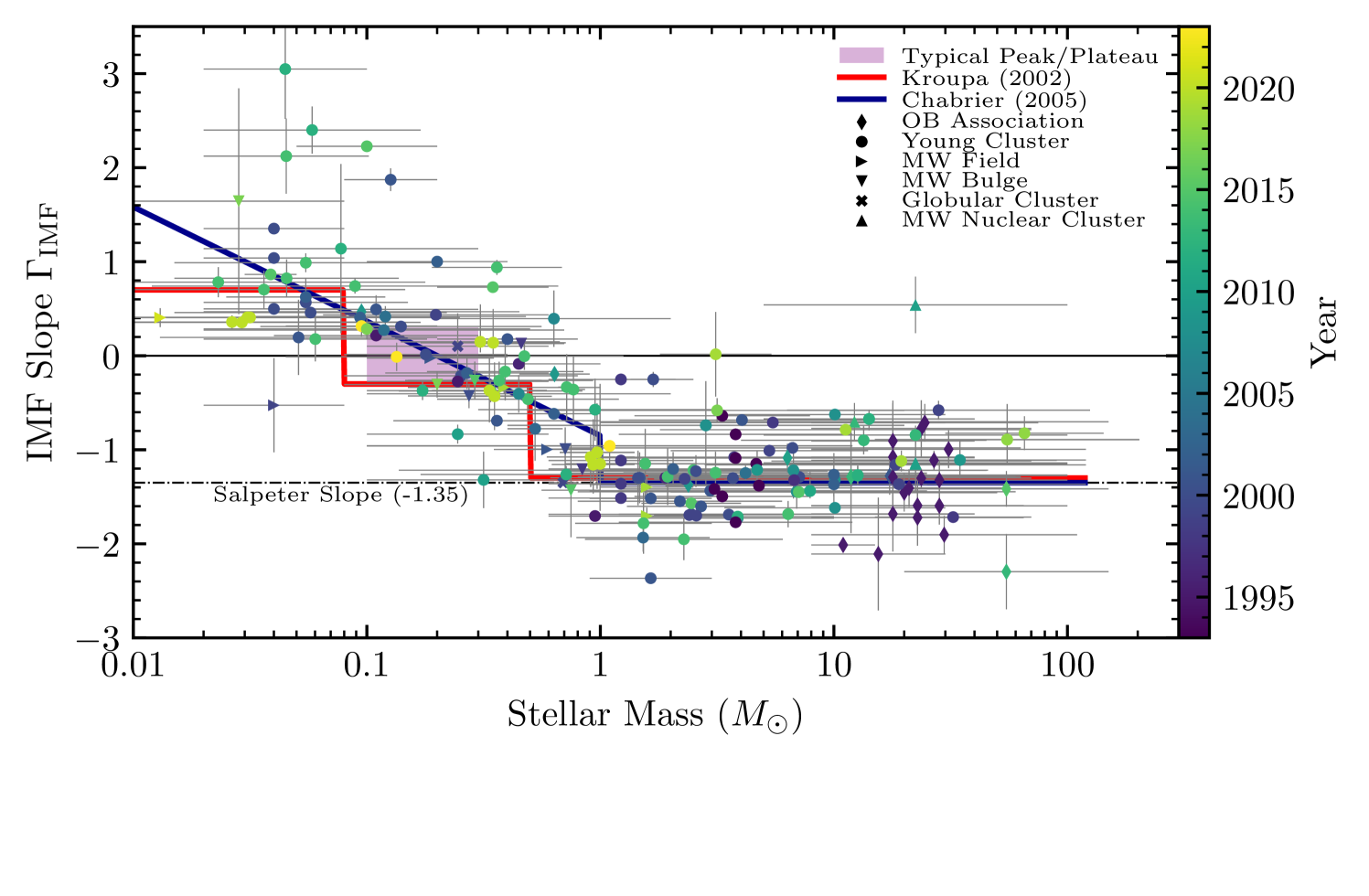
Hennebelle & Grudić [12] summarized a large number of observed slopes and plotted Figure 1. It can be seen that when the stellar mass is greater than 1 solar mass, lies between 0 and -2, corresponding to between 1 and 3; when the mass is smaller, gradually approaches 2. If these very low-mass stars form in an environment where the gas is so severely deficient that E(V) approaches 1, it can explain the observed slope. As for the slope-mass relation in the figure, it may represent a transition from when E(v) is much greater than 1 to when E(V) is close to 1.
Moreover, the M in our derivation can be understood as the core mass (corresponding to the core mass function, CMF), or it can also be interpreted as the IMF, since both are within the same probabilistic framework. However, this does not imply that the theoretical predictions for their slopes are the same because when it comes to equation 13 and equation 14, the corrections that need to be introduced if the linear assumption is not adopted are different for the CMF and the IMF. The relationship between the IMF and the CMF requires further investigation [20], and the specific differences may lie in the corrections involving equation 13 and equation 14.
Acknowledgements.
This work is supported by funds from the author’s institution.References
- Salpeter [1955] E. E. Salpeter, The Luminosity Function and Stellar Evolution., Astrophys. J. 121, 161 (1955).
- Bastian et al. [2010] N. Bastian, K. R. Covey, and M. R. Meyer, A universal stellar initial mass function? a critical look at variations, Annual Review of Astronomy and Astrophysics 48, 339 (2010).
- Luhman [2012] K. L. Luhman, The formation and early evolution of low-mass stars and brown dwarfs, Annual Review of Astronomy and Astrophysics 50, 65 (2012).
- Smith [2020] R. J. Smith, Evidence for initial mass function variation in massive early-type galaxies, Annual Review of Astronomy and Astrophysics 58, 577 (2020).
- Bate [2019] M. R. Bate, The statistical properties of stars and their dependence on metallicity, Monthly Notices of the Royal Astronomical Society 484, 2341 (2019), https://academic.oup.com/mnras/article-pdf/484/2/2341/27635804/stz103.pdf .
- Chon et al. [2022] S. Chon, H. Ono, K. Omukai, and R. Schneider, Impact of the cosmic background radiation on the initial mass function of metal-poor stars, Monthly Notices of the Royal Astronomical Society 514, 4639 (2022), https://academic.oup.com/mnras/article-pdf/514/3/4639/44743703/stac1549.pdf .
- Guszejnov et al. [2022] D. Guszejnov, M. Y. Grudić, S. S. R. Offner, C.-A. Faucher-Giguère, P. F. Hopkins, and A. L. Rosen, Effects of the environment and feedback physics on the initial mass function of stars in the starforge simulations, Monthly Notices of the Royal Astronomical Society 515, 4929 (2022), https://academic.oup.com/mnras/article-pdf/515/4/4929/45471309/stac2060.pdf .
- Tanvir and Krumholz [2023] T. S. Tanvir and M. R. Krumholz, The metallicity dependence of the stellar initial mass function, Monthly Notices of the Royal Astronomical Society 527, 7306 (2023), https://academic.oup.com/mnras/article-pdf/527/3/7306/54348842/stad3581.pdf .
- Heger et al. [2023] A. Heger, B. Müller, and I. Mandel, In the encyclopedia of cosmology (set 2): Frontiers in cosmology, vol. 3, black holes, ed, Z Haiman , 61 (2023).
- Kroupa et al. [2013] P. Kroupa, C. Weidner, J. Pflamm-Altenburg, I. Thies, J. Dabringhausen, M. Marks, and T. Maschberger, The Stellar and Sub-Stellar Initial Mass Function of Simple and Composite Populations, in Planets, Stars and Stellar Systems. Volume 5: Galactic Structure and Stellar Populations, Vol. 5, edited by T. D. Oswalt and G. Gilmore (2013) p. 115.
- Hopkins [2018] A. M. Hopkins, The Dawes Review 8: Measuring the Stellar Initial Mass Function, Publications of the Astronomical Society of Australia 35, e039 (2018), arXiv:1807.09949 [astro-ph.GA] .
- Hennebelle and Grudić [2024] P. Hennebelle and M. Grudić, The physical origin of the stellar initial mass function, Annual Review of Astronomy and Astrophysics 62, 63 (2024).
- Tielens [2005] A. G. Tielens, The physics and chemistry of the interstellar medium (Cambridge University Press, 2005).
- Klessen and Glover [2023] R. S. Klessen and S. C. Glover, The first stars: Formation, properties, and impact, Annual Review of Astronomy and Astrophysics 61, 65 (2023).
- Hennebelle and Falgarone [2012] P. Hennebelle and E. Falgarone, Turbulent molecular clouds, Astron. Astrophys. Rev. 20 (2012).
- Smith et al. [2014] R. J. Smith, S. C. O. Glover, and R. S. Klessen, On the nature of star-forming filaments – i. filament morphologies, Monthly Notices of the Royal Astronomical Society 445, 2900 (2014), https://academic.oup.com/mnras/article-pdf/445/3/2900/13766770/stu1915.pdf .
- Zhao et al. [2020] B. Zhao, K. Tomida, P. Hennebelle, J. J. Tobin, A. Maury, T. Hirota, Á. Sánchez-Monge, R. Kuiper, A. Rosen, A. Bhandare, M. Padovani, and Y.-N. Lee, Formation and evolution of disks around young stellar objects, Space Sci. Rev. 216, 43 (2020).
- Colman and Teyssier [2020] T. Colman and R. Teyssier, On the origin of the peak of the stellar initial mass function: exploring the tidal screening theory, Monthly Notices of the Royal Astronomical Society 492, 4727 (2020), https://academic.oup.com/mnras/article-pdf/492/4/4727/32322408/staa075.pdf .
- Grudić et al. [2022] M. Y. Grudić, D. Guszejnov, S. S. R. Offner, A. L. Rosen, A. N. Raju, C.-A. Faucher-Giguère, and P. F. Hopkins, The dynamics and outcome of star formation with jets, radiation, winds, and supernovae in concert, Monthly Notices of the Royal Astronomical Society 512, 216 (2022), https://academic.oup.com/mnras/article-pdf/512/1/216/42894596/stac526.pdf .
- Pelkonen et al. [2021] V.-M. Pelkonen, P. Padoan, T. Haugbølle, and A. Nordlund, From the cmf to the imf: beyond the core-collapse model, Monthly Notices of the Royal Astronomical Society 504, 1219 (2021), https://academic.oup.com/mnras/article-pdf/504/1/1219/37309813/stab844.pdf .