Nonlinear Modeling and Observability of a Planar Multi-Link Robot with Link Thrusters*

Abstract

This work is motivated by the development of cooperative teams of small, soft underwater robots designed to accomplish complex tasks through collective behavior. These robots take inspiration from biology: salps are gelatinous, jellyfish-like marine animals that utilize jet propulsion for maneuvering and can physically connect to form dynamic chains of arbitrary shape and size. The primary contributions of this research are twofold: first, we adapt a planar nonlinear multi-link snake robot model to model a planar multi-link salp-inspired system by removing joint actuators, introducing link thrusters, and allowing for non-uniform link lengths, masses, and moments of inertia. Second, we conduct a nonlinear observability analysis of the multi-link system with link thrusters, showing that the link angles, angular velocities, masses, and moments of inertia are locally observable when equipped with inertial measurement units and operating under specific thruster conditions. This research provides a theoretical foundation for modeling and estimating both the state and intrinsic parameters of a multi-link system with link thrusters, which are essential for effective controller design and performance.

I INTRODUCTION

Large, expensive, and highly capable robots are increasingly being replaced by cooperative teams of smaller, less expensive robots that, through collaboration, can achieve comparable or even superior performance in various tasks. This work is motivated by advancements in underwater robotics, where remotely operated vehicles (ROVs) and autonomous underwater vehicles (AUVs) are widely used for inspection, mapping, and intervention tasks. In particular, this research is directed towards the next generation of small, flexible, and minimally capable underwater vehicles bio-inspired by salps [1, 2]—gelatinous marine organisms roughly the size and shape of a soda can that maneuver using jet propulsion by pumping water through their bodies.

A distinctive feature of both salps and their bio-inspired multi-link robotic counterparts is their ability to physically connect, forming long, flexible chains—often consisting of dozens of units—that dynamically reshape into structures such as spirals, rings, and arcs. Significant progress has been made in developing underwater soft robotic mechanisms that replicate the jet propulsion of salps [3, 4]. However, the challenges of modeling, accurately measuring, and controlling the state of these systems remain an open area of research.

Observability is a necessary property for any system because it determines whether an estimator can uniquely reconstruct the system’s state from available measurements, which is essential for safe and efficient controller design. While intrinsic properties, such as mass, inertia, etc., can be measured in a laboratory setting for minimally configurable rigid-body systems, they become significantly more challenging and costly to measure for multi-link and underwater systems. For example, in underwater vehicles, added mass—the resistance due to accelerating through a fluid—is typically measured by towing the vehicle through the water at different speeds. However, this approach is infeasible for a multi-link system, as their size and shape are arbitrary and dynamic. Instead of relying on pre-deployment experiments, it is, therefore, desirable to have a multi-link system that can estimate its pose (position and orientation) and intrinsic properties in real-time.

The primary contributions of this work are twofold. First, we adapt a nonlinear multi-link snake robot model to suit a salp-inspired multi-link system with link thrusters. In the realm of freely moving multi-link robots, the research on snake robots has been the most comparable to salp-inspired systems. Extensive model development, controller design, and analysis for terrestrial and underwater snake robots are presented in [5, 6].

The second key contribution is a nonlinear observability analysis of the salp-inspired multi-link model with inertial measurement units (IMUs), showing that link angles, angular velocities, masses, and moments of inertia are locally observable under specific thruster conditions. The research conducted in this work is the dual of the controllability analysis presented in [7], where a geometric mechanics approach is used for controllability and gait analyses. The results from [7] were validated on LandSalp, a kinematically representative three-link robot with wheels.

Previous research on rigid body intrinsic parameter estimation have employed nonlinear observability analyses, such as those conducted for a six-degree-of-freedom aircraft in [8, 9]. These analyses demonstrate that certain intrinsic aircraft parameters are observable using a single IMU and can be estimated in real-time, given specific external force conditions. Similarly, [10] presents an algorithm for estimating the mass, center of mass, and moment of inertia for each link in a fixed-base manipulator.

The structure of this paper is as follows: Section II introduces the salp-inspired nonlinear multi-link model with link thrusters. In Section III, the measurement function for an IMU is derived from the general equation governing the acceleration of a point in a rotating reference frame relative to an inertial frame. Section IV provides a brief overview of Lie derivatives and nonlinear observability. The main contribution of this work is presented in Section V, where a nonlinear observability analysis is conducted, and the conditions for observability are derived. Finally, Section VI summarizes the findings and future work.

II MULTI-LINK SYSTEM MODEL

Variable	Description	Vector	Matrix
$N$	Number of links	–	–
$l_{i}$	Half the length of link $i$	$\mathbf{l}\in\mathbb{R}^{N}_{>0}$	$\mathbf{L}=\operatorname{diag}(\mathbf{l})\in\mathbb{D}^{N}_{++}$
$m_{i}$	Mass of link $i$	$\mathbf{{m}}=\begin{bmatrix}\frac{1}{m_{1}}&\ldots&\frac{1}{m_{N}}\end{bmatrix}\in\mathbb{R}^{N}_{>0}$	$\mathbf{{M}}=\operatorname{diag}(\mathbf{{m}})\in\mathbb{D}^{N}_{++}$
$j_{i}$	Moment of inertia of link $i$	$\mathbf{j}\in\mathbb{R}^{N}_{>0}$	$\mathbf{J}=\operatorname{diag}(\mathbf{j})\in\mathbb{D}^{N}_{++}$
$\theta_{i}$	CCW angle from the inertial $x$-axis to link $i$ $x$-axis	$\bm{\theta}\in\mathbb{R}^{N}$	–
$(x_{i},y_{i})$	Inertial position of the CM of link $i$	$\mathbf{X},\mathbf{Y}\in\mathbb{R}^{N}$	–
$(p_{x},p_{y})$	Inertial position of the CM of the multi-link system	$\mathbf{p}\in\mathbb{R}^{2}$	–
$u_{i}$	Thruster force on link $i$	$\mathbf{u}\in\mathbb{R}^{N}$	–
$\psi_{i}$	CCW angle from the link $i$ $x$-axis to thrust vector $u_{i}$	$\bm{\psi}\in\mathbb{R}^{N}$	–
$(f_{x,i},f_{y,i})$	Net inertial frame $x$ and $y$ forces on link $i$	$\mathbf{f}_{x},\mathbf{f}_{y}\in\mathbb{R}^{N}$	–

TABLE I: Variables and their associated vectors and matrices [5].

The multi-link system model presented in this section is adapted from and inspired by the underwater multi-link snake robot model in [5, 6]. Each “link” in our model corresponds to an individual salp robot equipped with a jet thruster and an independent electronics and sensor suite, capable of forming chains of arbitrary length and configuration. Our multi-link salp model differs from the snake model in the following key aspects:

1. Joints are unactuated

2. Controlled thruster forces are applied at the center of mass (CM) of each link

3. Mass, length, and moment of inertia are not assumed to be identical across links

For brevity, we do not present the full derivation of the salp model here; however, a detailed derivation of the snake model can be found in [5].

The system state vector is defined as

$$\mathbf{x}=\begin{bmatrix}\bm{\theta}&\mathbf{p}&\dot{\bm{\theta}}&\dot{\mathbf{p}}\end{bmatrix}\in\mathbb{R}^{2N+4},$$ (1)

where $\theta_{i}$ denotes the angle of the link $i$ $x$-axis relative to the inertial $x$-axis, with counterclockwise (CCW) considered positive. The vector $\mathbf{p}$ represents the $x$-$y$ position of the multi-link system’s CM. We define the following sets of $N\times N$ matrices: symmetric matrices $\mathbb{S}^{N}$, symmetric positive definite matrices $\mathbb{S}^{N}_{++}$, skew-symmetric matrices $\mathbb{S}^{N}_{\times}$, diagonal matrices $\mathbb{D}^{N}$, and diagonal positive definite matrices $\mathbb{D}^{N}_{++}$. Table I summarizes all relevant variables, including their scalar, vector, and matrix representations. Corresponding free-body diagrams for the multi-link system and a single link are shown in Figures 1 and 2. The axes of the link body frame are alternatively referred to as the tangent ($x_{\text{link},i}$) and normal ($y_{\text{link},i}$) directions and the CM of the link is the origin of the link frame.

Figure 1: Multi-link free body diagram.

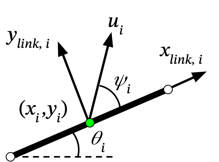
Figure 2: Single link free body diagram.

The following matrices, frequently used in the derivation of the system model, are defined for conciseness:

$$\mathbf{A} =\begin{bmatrix}1&1&0&0&0\\ 0&\cdot&\cdot&0&0\\ 0&0&\cdot&\cdot&0\\ 0&0&0&1&1\end{bmatrix}\in\mathbb{R}^{(N-1)\times N}$$ (2)

$$\mathbf{D} =\begin{bmatrix}1&-1&0&0&0\\ 0&\cdot&\cdot&0&0\\ 0&0&\cdot&\cdot&0\\ 0&0&0&1&-1\end{bmatrix}\in\mathbb{R}^{(N-1)\times N}$$ (3)

$$\mathbf{E} =\left[\begin{array}[]{cc}\mathbf{1}_{N}&\mathbf{0}_{N\times 1}\\ \mathbf{0}_{N\times 1}&\mathbf{1}_{N}\end{array}\right]\in\mathbb{R}^{2N\times 2}$$ (6)

$$\mathbf{V} ={\mathbf{A}}^{\top}\left(\mathbf{D}{\mathbf{{M}}}{\mathbf{D}}^{\top}\right)^{-1}\mathbf{A}\in\mathbb{S}^{N}$$ (7)

$$\mathbf{K} ={\mathbf{A}}^{\top}\left(\mathbf{D}{\mathbf{{M}}}{\mathbf{D}}^{\top}\right)^{-1}\mathbf{D}\in\mathbb{R}^{N\times N}$$ (8)

$$\mathbf{M}_{\theta} =\mathbf{J}+\mathbf{L}\left(\mathbf{S}_{\bm{\theta}}\mathbf{V}\mathbf{S}_{\bm{\theta}}+\mathbf{C}_{\bm{\theta}}\mathbf{V}\mathbf{C}_{\bm{\theta}}\right)\mathbf{L}\in\mathbb{S}^{N}_{++}$$ (9)

$$\mathbf{W} =\mathbf{L}\left(\mathbf{S}_{\bm{\theta}}\mathbf{VC}_{\theta}-\mathbf{C}_{\bm{\theta}}\mathbf{VS}_{\theta}\right)\mathbf{L}\in\mathbb{S}^{N}_{\times}.$$ (10)

Here, $\mathbf{1}_{N}$ is an $N$-dimensional vector of ones, $\mathbf{I}_{N}$ is the $N\times N$ identity matrix, $\mathbf{C}_{\bm{\theta}}=\operatorname{diag}(\cos\boldsymbol{\theta})\in\mathbb{D}^{N}$, and $\mathbf{S}_{\bm{\theta}}=\operatorname{diag}(\sin\boldsymbol{\theta})\in\mathbb{D}^{N}$.

The nonlinear dynamics of the multi-link system are given by

$$\dot{\mathbf{x}}=\begin{bmatrix}\dot{\bm{\theta}}\\ \dot{\mathbf{p}}\\ \mathbf{M}_{\theta}^{-1}\left(-\mathbf{W}\dot{\bm{\theta}}^{2}+\mathbf{L}\mathbf{S}_{\bm{\theta}}\mathbf{K}{\mathbf{{M}}}\mathbf{f}_{x}-\mathbf{L}\mathbf{C}_{\bm{\theta}}\mathbf{K}{\mathbf{{M}}}\mathbf{f}_{y}\right)\\ \frac{1}{m_{\Sigma}}{\mathbf{E}}^{\top}\mathbf{f}\end{bmatrix},$$ (11)

where $\mathbf{f}=\begin{bmatrix}\mathbf{f}_{x}&\mathbf{f}_{y}\end{bmatrix}\in\mathbb{R}^{2N}$, $\dot{\boldsymbol{\theta}}^{2}=\begin{bmatrix}\dot{\theta}_{1}^{2}&\ldots&\dot{\theta}_{N}^{2}\end{bmatrix}$ and $m_{\Sigma}=\sum_{i=1}^{N}m_{i}$ is the total mass of the multi-link system. The net forces consist of external forces and thruster forces:

$$\mathbf{f}_{x}=\mathbf{f}_{ext,x}+\mathbf{C}_{\bm{\theta+\psi}}\mathbf{u},\quad\mathbf{f}_{y}=\mathbf{f}_{ext,y}+\mathbf{S}_{\bm{\theta+\psi}}\mathbf{u},$$ (12)

where $\mathbf{C}_{\bm{\theta+\psi}}=\operatorname{diag}(\cos(\bm{\theta+\bm{\psi}}))\in\mathbb{D}^{N}$ and $\mathbf{S}_{\bm{\theta+\psi}}=\operatorname{diag}(\sin(\bm{\theta+\bm{\psi}}))\in\mathbb{D}^{N}$. In this work, we do not assume any specific models for the external forces $\mathbf{f}_{ext,x}$ and $\mathbf{f}_{ext,y}$, which may include hydrodynamic, gravitational, and frictional forces depending on the application.

The CM of the multi-link system is calculated by

$$\mathbf{p}=\begin{bmatrix}p_{x}\\ p_{y}\end{bmatrix}=\frac{1}{m_{\Sigma}}\begin{bmatrix}\mathbf{{m}}^{-\top}\mathbf{X}\\ \mathbf{{m}}^{-\top}\mathbf{Y}\end{bmatrix},$$ (13)

where $\mathbf{{m}}^{-1}=\begin{bmatrix}m_{1}&\dots&m_{N}\end{bmatrix}$. The link positions and velocities can be reconstructed from the multi-link CM and link angles as follows:

$$\mathbf{T}=\begin{bmatrix}\mathbf{D}\\ \frac{1}{m_{\Sigma}}{\mathbf{{m}}^{-\top}}\end{bmatrix}\in\mathbb{R}^{N\times N}$$ (14)

$$\mathbf{X}=\mathbf{T}^{-1}\begin{bmatrix}-\mathbf{A}\mathbf{L}\cos(\bm{\theta})\\ p_{x}\end{bmatrix},\ \dot{\mathbf{X}}=\mathbf{T}^{-1}\begin{bmatrix}\mathbf{A}\mathbf{L}\mathbf{S}_{\bm{\theta}}\dot{\bm{\theta}}\\ \dot{p_{x}}\end{bmatrix}$$ (15)

$$\mathbf{Y}=\mathbf{T}^{-1}\begin{bmatrix}-\mathbf{A}\mathbf{L}\sin(\bm{\theta})\\ p_{y}\end{bmatrix},\ \dot{\mathbf{Y}}=\mathbf{T}^{-1}\begin{bmatrix}-\mathbf{A}\mathbf{L}\mathbf{C}_{\bm{\theta}}\dot{\bm{\theta}}\\ \dot{p_{y}}\end{bmatrix}.$$ (16)

III IMU MEASUREMENT MODEL

In this section, we derive the measurement function for an IMU placed on a link $i$ for the nonlinear system (11). A single IMU measures the total acceleration and angular velocity at its current location relative to an inertial frame. The measurement function we derive is written in terms of which link the IMU is attached to and its relative position to the center of mass of that link.

III-A Relative Motion

The total acceleration of a point in a rotating frame, as observed from an inertial frame, is given by

$$\mathbf{a}_{\text{inertial}} =\mathbf{a}_{\text{origin}}+\mathbf{a}_{\text{relative}}+2\boldsymbol{\omega}\times\mathbf{v}$$ (17)

$$\quad+\boldsymbol{\omega}\times(\boldsymbol{\omega}\times\mathbf{r})+\bm{\alpha}\times\mathbf{r}.$$

The variables are all in $\mathbb{R}^{3}$ and defined as:

• $\mathbf{a}_{\text{inertial}}$: Total acceleration of the point in the inertial frame

• $\mathbf{a}_{\text{origin}}$: Acceleration of the rotating frame’s origin relative to the inertial frame

• $\mathbf{a}_{\text{relative}}$: Acceleration of the point relative to the rotating frame

• $\mathbf{v}$: Velocity of the point relative to the rotating frame

• $\mathbf{r}$: Position vector of the point relative to the rotating frame’s origin

• $\boldsymbol{\omega}$: Angular velocity of the rotating frame relative to the inertial frame

• $\bm{\alpha}$: Angular acceleration of the rotating frame relative to the inertial frame

Equation (17) will be used as the starting point for deriving the IMU measurement equation in the next subsection.

III-B IMU Measurement

The measurement function for an IMU in 3D is

$$\mathbf{y}=h(\mathbf{x})=\begin{bmatrix}\mathbf{a}_{\text{inertial}}&\bm{\omega}\end{bmatrix}\in\mathbb{R}^{6}.$$ (18)

We will simplify this equation by first assuming that an IMU placed on link $i$ is fixed relative to the link frame, i.e., $\mathbf{r}=\text{constant}$, $\mathbf{v}=0$, and $\mathbf{a}_{\text{relative}}=0$. This simplifies (17) to

$$\mathbf{a}_{\text{inertial}}=\mathbf{a}_{\text{origin}}+\boldsymbol{\omega}\times(\boldsymbol{\omega}\times\mathbf{r})+\bm{\alpha}\times\mathbf{r}.$$ (19)

Next, since the multi-link system (11) is planar, the cross-product terms can be simplified. In 2D, $\boldsymbol{\omega}$ and $\bm{\alpha}$ are perpendicular to the plane (along the $z$-axis) and $\mathbf{r}\in\mathbb{R}^{2}$, so the simplified equation after the planar assumption is:

$$\mathbf{a}_{\text{inertial}}=\mathbf{a}_{\text{origin}}-\omega^{2}\mathbf{r}+\alpha\begin{bmatrix}0&-1\\ 1&0\end{bmatrix}\mathbf{r},$$ (20)

where $\omega=|\bm{\omega}|_{2}$ and $\alpha=|\bm{\alpha}|_{2}$.

The net forces applied at the CM of link $i$ in inertial frame coordinates are $\mathbf{f}_{i}=\begin{bmatrix}f_{x,i}&f_{y,i}\end{bmatrix}\in\mathbb{R}^{2}$. The acceleration at the CM of the link is proportional to the net forces applied at the CM divided by the link mass: $\mathbf{a}_{\text{origin}}=\frac{{\mathbf{f}}_{i}}{m_{i}}$. Lastly, substituting in the appropriate terms, the measurement function for an IMU on link $i$ is

$$\mathbf{y}_{i} =h_{i}(\mathbf{x})=\begin{bmatrix}\frac{{\mathbf{f}}_{i}}{m_{i}}-\dot{\theta}_{i}^{2}\mathbf{r}+\ddot{\theta}_{i}\begin{bmatrix}0&-1\\ 1&0\end{bmatrix}\mathbf{r}\\ \dot{\theta}_{i}\end{bmatrix}\in\mathbb{R}^{3}.$$ (21)

IV NONLINEAR OBSERVABILITY

For linear systems, observability has a single well-defined meaning. However, in nonlinear systems, observability can exist in varying degrees, requiring a precise definition of the specific type being considered. Below, we provide a brief review of nonlinear observability and the Lie algebraic approach for determining the observability of nonlinear systems, summarized from [11, 12, 13].

Consider the nonlinear system, $\Sigma$, with the following process and measurement models:

$$\Sigma:\quad\dot{\mathbf{x}}=f(\mathbf{x},\mathbf{u}),\quad\mathbf{y}=h(\mathbf{x}),$$ (22)

where $\mathbf{x}(t)\in\mathbb{R}^{n}$, $\mathbf{y}(t)\in\mathbb{R}^{k}$, and $\mathbf{u}(t)\in\mathcal{U}\subseteq\mathbb{R}^{m}$, with $\mathcal{U}$ the set of admissible controls. Let $\mathbf{x}(t,\mathbf{x}_{0},\mathbf{u})$ denote the solution to the initial value problem for $\Sigma$ with initial condition $\mathbf{x}(0)=\mathbf{x}_{0}$ under the control input $\mathbf{u}(t)$, and define $\mathbf{y}(t,\mathbf{x}_{0},\mathbf{u})=h(\mathbf{x}(t,\mathbf{x}_{0},\mathbf{u}))$.

Local observability is defined as follows: $\mathbf{x}_{0}$ and $\mathbf{x}_{1}$ are $V$-indistinguishable if, for every control $\mathbf{u}\in\mathcal{U}$, the corresponding state trajectories $\mathbf{x}(t,\mathbf{x}_{0},\mathbf{u})$ and $\mathbf{x}(t,\mathbf{x}_{1},\mathbf{u})$ remain in $V\subseteq\mathbb{R}^{n}$ over $t\in[0,T]$ and satisfy

$$\mathbf{y}(t,\mathbf{x}_{0},\mathbf{u})=\mathbf{y}(t,\mathbf{x}_{1},\mathbf{u})\ \forall\ t\in[0,T].$$

The system $\Sigma$ is locally observable at $\mathbf{x}_{0}$ if there exists a neighborhood $W$ of $\mathbf{x}_{0}$ such that, for every neighborhood $V\subset W$, indistinguishability within $V$ implies $\mathbf{x}_{0}=\mathbf{x}_{1}$. If $\Sigma$ is locally observable at all $\mathbf{x}$, then it is locally observable. Intuitively, this definition means that $\mathbf{x}_{0}$ can be distinguished from nearby states within finite time and with trajectories remaining close to $\mathbf{x}_{0}$.

A differential geometric approach to testing observability involves analyzing the Lie derivatives of the output function $h(\mathbf{x})$ with respect to the process model $f(\mathbf{x})$. The zeroth through second-order Lie derivatives are given by:

$$\mathcal{L}_{f}^{0}h =h(\mathbf{x}),$$ (23)

$$\mathcal{L}_{f}^{1}h =\nabla h(\mathbf{x})\cdot f(\mathbf{x}),$$ (24)

$$\mathcal{L}_{f}^{2}h =\nabla(\mathcal{L}_{f}^{1}h)\cdot f(\mathbf{x})=\mathcal{L}_{f}^{1}\left(\mathcal{L}_{f}^{1}h\right).$$ (25)

If $h(\mathbf{x})$ is a scalar function, $\nabla h(\mathbf{x})$ is its gradient (a row vector). If $h(\mathbf{x})$ is a vector function, $\nabla h(\mathbf{x})$ is the Jacobian matrix. Higher-order Lie derivatives follow a similar recursive form.

If the process model is control-affine, meaning it decomposes as: $\dot{\mathbf{x}}=f_{0}(\mathbf{x})+\sum_{i=1}^{m}f_{i}(\mathbf{x})u_{i}$, where $f_{0}$ represents the drift term, then Lie derivatives can be computed separately with respect to the drift and control vector fields. For instance, a second-order mixed Lie derivative of $h(\mathbf{x})$, first along $f_{0}$ and then along $f_{1}$, is:

$$\mathcal{L}_{f_{1}f_{0}}^{2}h(\mathbf{x})=\mathcal{L}_{f_{1}}^{1}(\mathcal{L}_{f_{0}}^{1}h(\mathbf{x}))=\nabla(\mathcal{L}_{f_{0}}^{1}h(\mathbf{x}))\cdot f_{1}(\mathbf{x}).$$ (26)

Taking a Lie derivative with respect to $f_{i}(\mathbf{x})$ implicitly assumes $u_{i}\neq 0$.

The observability Lie algebra $\mathcal{O}$, or observation space, for a control-affine system $\Sigma$ is

$$\mathcal{O}=\text{span}\left\{\mathcal{L}_{f_{i}}^{d}h(\mathbf{x})\mid d\in\mathbb{N}_{0},\;i=0,\dots,m\right\}.$$ (27)

Here, $f_{i}$ can be any Lie derivative combination of the control-affine process model functions. Observability is then determined using the following rank condition:

Theorem 1.

The nonlinear system is locally observable if $\operatorname{rank}(\text{d}\mathcal{O})=n$ [11].

There is no universal method for constructing $\text{d}\mathcal{O}$, but in practice, sequentially computing Lie derivatives along well-chosen combinations of the process model functions often yield good results. If any set of Lie derivatives satisfies the rank condition then the system is locally observable.

V OBSERVABILITY ANALYSIS

Our goal is to establish the observability conditions for the state of the multi-link system (11) along with a set of intrinsic parameters. For this analysis, we make the following assumptions:

1. The length of each link ($l_{i}$) is known

2. The mass ($m_{i}$) and inertia ($j_{i}$) of each link are treated as independent variables

3. Thruster angles ($\psi_{i}$) are fixed relative to the link frame

4. Non-zero link thrusts ($u_{i}\neq 0$)

5. One IMU placed at the CM of each link

The intrinsic parameters this analysis is concerned with are the mass and inertia of each link. In practice, the position and velocity of the multi-link system can be recovered given some initial position and velocity estimate and by time-differencing the IMU measurements, so they will be omitted from the state for the observability analysis. The augmented state vector and process model are:

$$\mathbf{x}_{\text{aug}}=\begin{bmatrix}\bm{\theta}&\dot{\bm{\theta}}&\mathbf{{m}}&\mathbf{j}\end{bmatrix}\in\mathbb{R}^{4N}$$ (28)

$$\dot{\mathbf{x}}_{\text{aug}}=\begin{bmatrix}\dot{\bm{\theta}}\\ \mathbf{M}_{\theta}^{-1}\left(-\mathbf{W}\dot{\bm{\theta}}^{2}+\mathbf{L}\mathbf{S}_{\bm{\theta}}\mathbf{K}{\mathbf{{M}}}\mathbf{f}_{x}-\mathbf{L}\mathbf{C}_{\bm{\theta}}\mathbf{K}{\mathbf{{M}}}\mathbf{f}_{y}\right)\\ \mathbf{0}_{N}\\ \mathbf{0}_{N}\end{bmatrix}.$$ (29)

The dynamics can be written in a control affine form with the control input function for thruster $i$ as

$$f_{i}(\mathbf{x}_{\text{aug}})=\begin{bmatrix}\mathbf{0}_{N}\\ \mathbf{M}_{\theta}^{-1}\mathbf{L}\left(\mathbf{S}_{\bm{\theta}}\mathbf{K}\mathbf{C}_{\bm{\theta+\psi}}-\mathbf{C}_{\bm{\theta}}\mathbf{K}\mathbf{S}_{\bm{\theta+\psi}}\right)\mathbf{{M}}\mathbf{e}_{i}\\ \mathbf{0}_{N}\\ \mathbf{0}_{N}\end{bmatrix}.$$ (30)

By assuming the IMU is placed at the CM of the link ($\mathbf{r}=\mathbf{0}$) in the measurement equation (21), the simplified measurement equation for an IMU at the CM of link $i$ is

$$h_{i}(\mathbf{x})=\begin{bmatrix}\frac{f_{x,i}}{m_{i}}&\frac{f_{y,i}}{m_{i}}&\dot{\theta}_{i}\end{bmatrix}\in\mathbb{R}^{3}.$$ (31)

If we assume an IMU at the CM of each link, concatenate and rearrange the rows then the measurement vector is

$$h(\mathbf{x})=\begin{bmatrix}{\mathbf{{M}}}\mathbf{f}_{x}\\ {\mathbf{{M}}}\mathbf{f}_{y}\\ \dot{\bm{\theta}}\end{bmatrix}=\begin{bmatrix}\mathbf{{M}}(\mathbf{f}_{ext,x}+\mathbf{C}_{\bm{\theta+\psi}}\mathbf{u})\\ \mathbf{{M}}(\mathbf{f}_{ext,y}+\mathbf{S}_{\bm{\theta+\psi}}\mathbf{u})\\ \dot{\bm{\theta}}\end{bmatrix}\in\mathbb{R}^{3N}.$$ (32)

V-A State Transformation

We will first apply a transformation to the state to simplify the Lie derivatives. Let the transformed state be $\mathbf{x}_{\text{aug}}^{\prime}=\mathcal{T}(\mathbf{x}_{\text{aug}})\in\mathbb{R}^{4N}$ where

$$\mathbf{x}_{\text{aug}}^{\prime} =\begin{bmatrix}\bm{\theta}&\bm{\nu}&\mathbf{{m}}&\mathbf{j}\end{bmatrix}$$ (33)

and $\bm{\nu}=\mathbf{M}_{\theta}^{-1}\mathbf{J}^{-1}\dot{\bm{\theta}}$. The transformation $\mathcal{T}(\mathbf{x}_{\text{aug}})$ is a diffeomorphism and if $\mathbf{x}_{\text{aug}}^{\prime}$ is observable, then $\mathbf{x}_{\text{aug}}$ is observable. The measurement is rewritten in terms of $\mathbf{x}_{\text{aug}}^{\prime}$ by substituting the transformed state variable $\dot{\bm{\theta}}=\mathbf{J}\mathbf{M}_{\theta}\bm{\nu}$:

$$h(\mathbf{x}_{\text{aug}}^{\prime})=\begin{bmatrix}\mathbf{{M}}(\mathbf{f}_{ext,x}+\mathbf{C}_{\bm{\theta+\psi}}\mathbf{u})\\ \mathbf{{M}}(\mathbf{f}_{ext,y}+\mathbf{S}_{\bm{\theta+\psi}}\mathbf{u})\\ \mathbf{J}\mathbf{M}_{\theta}\bm{\nu}\end{bmatrix}\in\mathbb{R}^{3N}.$$ (34)

The Lie derivatives are taken with respect to the transformed state $\mathbf{x}_{\text{aug}}^{\prime}$ in the remainder of the analysis.

V-B Zeroth-Order Lie Derivative

The zeroth order Lie derivative is the Jacobian of the measurement function. The $*$ is used to denote non-zero blocks that are omitted and assumed to be zero to simplify the analysis.

$$\mathcal{L}^{0}h =h(\mathbf{x}_{\text{aug}}^{\prime})$$ (35)

$$\nabla\mathcal{L}^{0}h =\begin{bmatrix}\mathbf{\Delta}_{1}&\mathbf{0}_{2N\times N}&\mathbf{\Delta}_{2}&\mathbf{0}_{2N\times N}\\ \mathbf{0}_{N\times N}&\mathbf{J}\mathbf{M}_{\theta}&\mathbf{0}_{N\times N}&*\end{bmatrix}$$ (36)

$$\mathbf{\Delta}_{1} =\begin{bmatrix}-\mathbf{{M}}\mathbf{S}_{\bm{\theta+\psi}}\operatorname{diag}(\mathbf{u})\\ \mathbf{{M}}\mathbf{C}_{\bm{\theta+\psi}}\operatorname{diag}(\mathbf{u})\end{bmatrix}\in\mathbb{R}^{2N\times N}$$ (37)

$$\mathbf{\Delta}_{2} =\begin{bmatrix}\operatorname{diag}(\mathbf{f}_{ext,x}+\mathbf{C}_{\bm{\theta+\psi}}\mathbf{u})\\ \operatorname{diag}(\mathbf{f}_{ext,y}+\mathbf{S}_{\bm{\theta+\psi}}\mathbf{u})\end{bmatrix}\in\mathbb{R}^{2N\times N}.$$ (38)

V-C First-Order Lie Derivatives

First-order Lie derivatives are taken with respect to an arbitrary control vector field $f_{i}$.

$$\mathcal{L}_{f_{i}}^{1}h =\nabla h(\mathbf{x}_{\text{aug}}^{\prime})\cdot f_{i}(\mathbf{x}_{\text{aug}}^{\prime})$$ (39)

$$=\begin{bmatrix}\mathbf{0}_{N}\\ \mathbf{0}_{N}\\ \mathbf{J}\mathbf{L}\left(\mathbf{S}_{\bm{\theta}}\mathbf{K}\mathbf{C}_{\bm{\theta+\psi}}-\mathbf{C}_{\bm{\theta}}\mathbf{K}\mathbf{S}_{\bm{\theta+\psi}}\right)\mathbf{{M}}\mathbf{e}_{i}\end{bmatrix}$$ (40)

$$\nabla\mathcal{L}_{f_{i}}^{1}h =\begin{bmatrix}\mathbf{0}_{N\times N}&\mathbf{0}_{N\times N}&\mathbf{0}_{N\times N}&\mathbf{0}_{N\times N}\\ \mathbf{0}_{N\times N}&\mathbf{0}_{N\times N}&\mathbf{0}_{N\times N}&\mathbf{0}_{N\times N}\\ *&\mathbf{0}_{N\times N}&*&\mathbf{\Delta}_{3}\end{bmatrix}$$ (41)

$$\mathbf{\Delta}_{3} =\operatorname{diag}(\mathbf{L}\left(\mathbf{S}_{\bm{\theta}}\mathbf{K}\mathbf{C}_{\bm{\theta+\psi}}-\mathbf{C}_{\bm{\theta}}\mathbf{K}\mathbf{S}_{\bm{\theta+\psi}}\right)\mathbf{{M}}\mathbf{e}_{i}).$$ (42)

V-D Observability Space

By including all of the control vector fields in $\text{d}\mathcal{O}$, we implicitly assume that $u_{i}\neq 0$. The first-order Lie derivative with respect to the drift vector field $f_{0}$ is excluded from the analysis because the derivatives became analytically intractable. Including $f_{0}$ terms may lead to less conservative conditions, i.e., requiring less control, for observability than those derived in this analysis.

Constructing $\text{d}\mathcal{O}$ from the zeroth and first-order control Lie derivatives yields:

$$\text{d}\mathcal{O}=\begin{bmatrix}\nabla\mathcal{L}^{0}h\\ \nabla\mathcal{L}_{f_{1:N}}^{1}h\end{bmatrix}\in\mathbb{R}^{(3N+3N^{2})\times 4N}.$$ (43)

Compiling the blocks, removing zero block rows for simplicity, and swapping the first and third columns yields the diagonal block matrix $\text{d}\mathcal{O}$ in equation (44).

$$\text{d}\mathcal{O} =\begin{bmatrix}-\mathbf{{M}}\mathbf{S}_{\bm{\theta+\psi}}\operatorname{diag}(\mathbf{u})&\operatorname{diag}(\mathbf{f}_{ext,x}+\mathbf{C}_{\bm{\theta+\psi}}\mathbf{u})&\mathbf{0}_{N\times N}&\mathbf{0}_{N\times N}\\ \mathbf{{M}}\mathbf{C}_{\bm{\theta+\psi}}\operatorname{diag}(\mathbf{u})&\operatorname{diag}(\mathbf{f}_{ext,y}+\mathbf{S}_{\bm{\theta+\psi}}\mathbf{u})&\mathbf{0}_{N\times N}&\mathbf{0}_{N\times N}\\ \mathbf{0}_{N\times N}&\mathbf{0}_{N\times N}&\mathbf{J}\mathbf{M}_{\theta}&\mathbf{0}_{N\times N}\\ \mathbf{0}_{N\times N}&\mathbf{0}_{N\times N}&\mathbf{0}_{N\times N}&\operatorname{diag}(\mathbf{L}\left(\mathbf{S}_{\bm{\theta}}\mathbf{K}\mathbf{C}_{\bm{\theta+\psi}}-\mathbf{C}_{\bm{\theta}}\mathbf{K}\mathbf{S}_{\bm{\theta+\psi}}\right)\mathbf{{M}}\mathbf{e}_{1})\\ \vdots&\vdots&\vdots&\vdots\\ \mathbf{0}_{N\times N}&\mathbf{0}_{N\times N}&\mathbf{0}_{N\times N}&\operatorname{diag}(\mathbf{L}\left(\mathbf{S}_{\bm{\theta}}\mathbf{K}\mathbf{C}_{\bm{\theta+\psi}}-\mathbf{C}_{\bm{\theta}}\mathbf{K}\mathbf{S}_{\bm{\theta+\psi}}\right)\mathbf{{M}}\mathbf{e}_{N})\end{bmatrix}\in\mathbb{R}^{(3N+N^{2})\times 4N}$$ (44)

The matrix in (44) is expressed in the compact block diagonal form as

$$\text{d}\mathcal{O}=\begin{bmatrix}\mathbf{\Omega}_{1}&\mathbf{0}_{2N\times N}&\mathbf{0}_{2N\times N}\\ \mathbf{0}_{N\times 2N}&\mathbf{J}\mathbf{M}_{\theta}&\mathbf{0}_{N\times N}\\ \mathbf{0}_{N^{2}\times 2N}&\mathbf{0}_{N^{2}\times N}&\mathbf{\Omega}_{2}\end{bmatrix}.$$ (45)

If each diagonal block of $\text{d}\mathcal{O}$ is full rank, then the entire matrix is full rank [14]. The block $\mathbf{J}\mathbf{M}_{\theta}$ is trivially full rank because it is the product of positive definite matrices, so the task becomes proving that $\mathbf{\Omega}_{1}\in\mathbb{R}^{2N\times 2N}$ and $\mathbf{\Omega}_{2}\in\mathbb{R}^{N^{2}\times N}$ are full rank. The remainder of this subsection focuses on deriving conditions for $\mathbf{\Omega}_{1}$ and $\mathbf{\Omega}_{2}$ to be full rank so that $\text{d}\mathcal{O}$ is subsequently full rank.

V-D1 $\mathbf{\Omega}_{1}$ Analysis

To prove the rank of $\mathbf{\Omega}_{1}$ we will utilize the following theorem:

Theorem 2.

Let

$$\mathbf{M}=\begin{bmatrix}\mathbf{A}&\mathbf{B}\\ \mathbf{C}&\mathbf{D}\end{bmatrix}$$

be a block matrix where $\mathbf{A},\mathbf{B},\mathbf{C},\mathbf{D}\in\mathbb{R}^{N\times N}$ and $\mathbf{C}\mathbf{D}=\mathbf{D}\mathbf{C}$. Then, the determinant of $\mathbf{M}$ satisfies:

$$\det(\mathbf{M})=\det(\mathbf{A}\mathbf{D}-\mathbf{B}\mathbf{C})\ \cite[cite]{[\@@bibref{}{Silvester2000-ww}{}{}]}.$$

Since the blocks of $\mathbf{\Omega}_{1}$ are all diagonal matrices and square, they commute with each other, and we can apply Theorem 2 to compute the determinant of $\mathbf{\Omega}_{1}$. Factoring out $-\mathbf{{M}}$ and applying the identity $\mathbf{C}_{\bm{\theta+\psi}}^{2}+\mathbf{S}_{\bm{\theta+\psi}}^{2}=\mathbf{I}_{N}$ yields

$$\begin{gathered}\det(\mathbf{\Omega}_{1})=\det(-\mathbf{{M}})\det(\operatorname{diag}(\mathbf{u}^{2})\\ +\mathbf{C}_{\bm{\theta+\psi}}\operatorname{diag}(\mathbf{u})\operatorname{diag}(\mathbf{f}_{ext,x})+\mathbf{S}_{\bm{\theta+\psi}}\operatorname{diag}(\mathbf{u})\operatorname{diag}(\mathbf{f}_{ext,y})).\end{gathered}$$ (46)

The term $\det(-\mathbf{{M}})$ is always non-zero because $\mathbf{{M}}\in\mathbb{D}^{N}_{++}$, so it can be ignored for rank analysis purposes. In the other determinant term, the determinant is acting on a summation of diagonal matrices. The determinant of a diagonal matrix is the product of its diagonal entries, so the problem can be reduced to finding the conditions for each diagonal element to be non-zero.

The diagonal entries of the diagonal matrix sum are

$$u_{i}(u_{i}+\cos(\theta_{i}+\psi_{i})f_{ext,x,i}+\sin(\theta_{i}+\psi_{i})f_{ext,y,i}).$$ (47)

We are implicitly assuming $u_{i}\neq 0$ by including the control vector fields in $\text{d}\mathcal{O}$, so the element-wise condition for a non-zero determinant, and therefore a full rank $\mathbf{\Omega}_{1}$, becomes

$$u_{i}\neq-(\cos(\theta_{i}+\psi_{i})f_{ext,x,i}+\sin(\theta_{i}+\psi_{i})f_{ext,y,i}).$$ (48)

This constraint implies that, in addition to requiring nonzero thruster forces on each link ($u_{i}\neq 0$), each link must also experience a nonzero net force.

V-D2 $\mathbf{\Omega}_{2}$ Analysis

The block has the form of taking each column of $\mathbf{L}\left(\mathbf{S}_{\bm{\theta}}\mathbf{K}\mathbf{C}_{\bm{\theta+\psi}}-\mathbf{C}_{\bm{\theta}}\mathbf{K}\mathbf{S}_{\bm{\theta+\psi}}\right)\mathbf{{M}}$, diagonalizing it, and stacking the blocks. The block $\mathbf{\Omega}_{2}$ is full rank if $\mathbf{L}\left(\mathbf{S}_{\bm{\theta}}\mathbf{K}\mathbf{C}_{\bm{\theta+\psi}}-\mathbf{C}_{\bm{\theta}}\mathbf{K}\mathbf{S}_{\bm{\theta+\psi}}\right)\mathbf{{M}}$ does not have a row of zeros because the columns of $\mathbf{\Omega}_{2}$ will be linearly independent by construction.

Let $\mathbf{F}=\mathbf{S}_{\bm{\theta}}\mathbf{K}\mathbf{C}_{\bm{\theta+\psi}}-\mathbf{C}_{\bm{\theta}}\mathbf{K}\mathbf{S}_{\bm{\theta+\psi}}$. The diagonal structures of $\mathbf{C}_{\bm{\theta}},\mathbf{S}_{\bm{\theta}},\mathbf{C}_{\bm{\theta+\psi}}$, and $\mathbf{S}_{\bm{\theta+\psi}}$ allow the matrix products to be expressed in simple element terms where the subscript $ij$ represents the matrix element corresponding to the $i$-th row and $j$-th column. Applying the trigonometric identities

$$\sin(\alpha\pm\beta) =\sin\alpha\cos\beta\pm\cos\alpha\sin\beta$$ (49)

$$\cos(\alpha\pm\beta) =\cos\alpha\cos\beta\mp\sin\alpha\sin\beta$$

and combining terms reduces the elements of $\mathbf{F}$ to

$$\mathbf{F}_{ij}=\mathbf{K}_{ij}\sin((\theta_{i}-\theta_{j})-\psi_{j}).$$ (50)

The matrix $\mathbf{K}$ has rank $N-1$ and it is easy to verify that $\ker(\mathbf{K})=\{\mathbf{1}_{N}\}$ and $\text{coker}\left(\mathbf{K}\right)=\{\begin{bmatrix}1&-1&1&-1&\dots\end{bmatrix}\in\mathbb{R}^{N}\}$. From this information, we can conclude that $\mathbf{K}$ does not have a row or column of zeros because the basis vector $\mathbf{e}_{i}$ is not in either kernel subspace. We will use this information in the following theorem to prove that $\mathbf{F}$ does not have a row of zeros.

Theorem 3.

Let $\mathbf{K}\in\mathbb{R}^{N\times N}$ be a matrix with $\operatorname{rank}(\mathbf{K})=N-1$ and no row or column composed entirely of zeros. Define the matrix $\mathbf{F}$ with elements

$$\mathbf{F}_{ij}=\sin((\theta_{i}-\theta_{j})-\psi_{j})\,\mathbf{K}_{ij},$$

where $\sin(\psi_{i})\neq 0\ \forall\ i$. Then, $\mathbf{F}$ cannot have a row consisting entirely of zeros.

Proof.

Since $\operatorname{rank}(\mathbf{K})=N-1$ and $\mathbf{K}$ has no row or column of zeros, there exists a permutation matrix $\mathbf{P}$ that reorders the columns such that the permuted matrix $\mathbf{K}^{\prime}=\mathbf{K}\mathbf{P}$ has all nonzero diagonal entries. Let $\mathbf{F}^{\prime}$ be

$$\mathbf{F}^{\prime}_{ij}=\sin((\theta_{i}-\theta_{j})-\psi_{j})\,\mathbf{K}^{\prime}_{ij}.$$

We first show that $\mathbf{F}^{\prime}$ cannot have a row of all zeros. The diagonal elements for any row $i$ are

$$\mathbf{F}^{\prime}_{ii}=\sin((\theta_{i}-\theta_{i})-\psi_{i})\,\mathbf{K}^{\prime}_{ii}=-\sin(\psi_{i})\,\mathbf{K}^{\prime}_{ii}.$$

Assuming $\sin(\psi_{i})\neq 0$ and $\mathbf{K}^{\prime}_{ii}\neq 0$ by construction, it follows that $\mathbf{F}^{\prime}_{ii}\neq 0$ and therefore, no row of $\mathbf{F}^{\prime}$ is entirely zero.

Since $\mathbf{F}=\mathbf{F}^{\prime}\mathbf{P}^{-1}$ and $\mathbf{P}^{-1}$ is a permutation matrix, permuting the columns of $\mathbf{F}^{\prime}$ does not introduce any zero rows. Therefore, $\mathbf{F}$ cannot have a row of all zeros. ∎

The matrices $\mathbf{L}$ and $\mathbf{{M}}$ are both diagonal positive definite and will not introduce any zero rows in the product $\mathbf{L}\mathbf{F}\mathbf{{M}}$ and therefore we can conclude that $\mathbf{\Omega}_{2}$ is full rank if $\sin(\psi_{i})\neq 0\ \forall\ i$.

We now present the main observability result:

Theorem 4.

The augmented state $\mathbf{x}_{\text{aug}}$ is locally observable under the following control conditions:

1. Non-zero thrust normal component: $u_{i}\sin(\psi_{i})\neq 0\ \forall\ i$

2. Non-zero net force:
   $u_{i}\neq-\big{(}\cos(\theta_{i}+\psi_{i})f_{ext,x,i}+\sin(\theta_{i}+\psi_{i})f_{ext,y,i}\big{)}\ \forall\ i.$

Proof.

As shown in the previous subsections, both $\mathbf{\Omega}_{1}$ and $\mathbf{\Omega}_{2}$ are full-rank matrices. Since $\text{d}\mathcal{O}$ is a diagonal block matrix with full-rank diagonal blocks, it follows that $\text{d}\mathcal{O}$ itself is full-rank. Consequently, the transformed state $\mathbf{x}_{\text{aug}}^{\prime}$ is locally observable, and since a diffeomorphism exists between $\mathbf{x}_{\text{aug}}^{\prime}$ and $\mathbf{x}_{\text{aug}}$, it follows that $\mathbf{x}_{\text{aug}}$ is also locally observable. ∎

Theorem 4 establishes sufficient conditions for link angles, angular velocities, masses, and moments of inertia of system 11 to be estimated in real-time from IMUs placed at the CM of each link.

VI CONCLUSIONS

In this work, we developed a planar multi-link model with link thrusters that is representative of a chain of salp-inspired robots by modifying an existing snake robot model. We then derived the sensor measurement equation for an IMU placed on an arbitrary link and proved that the system’s link angles, angular velocities, masses, and moments of inertia are locally observable with control provided the conditions in Theorem 4 are met. In the near term, future work will focus on validating these results through hardware experiments using the LandSalp test platform [7]. In the long term, future work will explore how the observability results are affected when each salp/link is modeled as a soft, flexible robotic structure rather than the rigid-body assumption used in this study.

References

- [1] A. Villanueva, C. Smith, and S. Priya, “A biomimetic robotic jellyfish (robojelly) actuated by shape memory alloy composite actuators,” Bioinspir. Biomim., vol. 6, p. 036004, Sept. 2011.
- [2] V. L. Gatto, J. M. Rossiter, and H. Hauser, “Robotic jellyfish actuated by soft FinRay effect structured tentacles,” in 2020 3rd IEEE International Conference on Soft Robotics (RoboSoft), pp. 144–149, IEEE, May 2020.
- [3] A. Jones and J. R. Davidson, “Underwater salp-inspired soft structure contraction with twisted coiled actuators,” in 2024 IEEE 7th International Conference on Soft Robotics (RoboSoft), pp. 504–510, IEEE, Apr. 2024.
- [4] Z. Yang, D. Chen, D. J. Levine, and C. Sung, “Origami-inspired robot that swims via jet propulsion,” IEEE Robot. Autom. Lett., vol. 6, pp. 7145–7152, Oct. 2021.
- [5] P. Liljeback, K. Y. Pettersen, O. Stavdahl, and J. T. Gravdahl, Snake robots: Modelling, mechatronics, and control. Advances in industrial control, London, England: Springer, 2013 ed., June 2012.
- [6] E. Kelasidi, K. Y. Pettersen, J. T. Gravdahl, and P. Liljeback, “Modeling of underwater snake robots,” in 2014 IEEE International Conference on Robotics and Automation (ICRA), IEEE, May 2014.
- [7] Y. Yanhao, L. H. Nina, S.-M. Yousef, J. Nathan, A. T. Zachary, R. Farhan, and L. H. Ross, “Geometric data-driven multi-jet locomotion inspired by salps,” arXiv [cs.RO], Mar. 2025.
- [8] B. Boyacioglu, D. Sandursky, and K. A. Morgansen, “Nonlinear estimation of rigid body inertial parameters,” in AIAA SCITECH 2023 Forum, (Reston, Virginia), American Institute of Aeronautics and Astronautics, Jan. 2023.
- [9] E. Sundquist, C. Whitehair, and K. A. Morgansen, “Nonlinear multi-sensor observability and estimation of rigid body inertial parameters,” in AIAA SCITECH 2024 Forum, (Reston, Virginia), American Institute of Aeronautics and Astronautics, Jan. 2024.
- [10] C. An, C. Atkeson, and J. Hollerbach, “Estimation of inertial parameters of rigid body links of manipulators,” in 1985 24th IEEE Conference on Decision and Control, IEEE, Dec. 1985.
- [11] R. Hermann and A. Krener, “Nonlinear controllability and observability,” IEEE Trans. Automat. Contr., vol. 22, pp. 728–740, Oct. 1977.
- [12] H. Nijmeijer and A. J. van der Schaft, Nonlinear Dynamical Control Systems. Springer Science & Business Media, Apr. 1990.
- [13] F. M. Mirzaei and S. I. Roumeliotis, “A kalman filter-based algorithm for IMU-camera calibration: Observability analysis and performance evaluation,” IEEE Trans. Robot., vol. 24, pp. 1143–1156, Oct. 2008.
- [14] J. R. Silvester, “Determinants of block matrices,” Math. Gaz., vol. 84, pp. 460–467, Nov. 2000.