Birational Geometry of Special Quotient Foliations and Chazy’s Equations

Abstract.

The works of Brunella and Santos have singled out three special singular holomorphic foliations on projective surfaces having invariant rational nodal curves of positive self-intersection. These foliations can be described as quotients of foliations on some rational surfaces under cyclic groups of transformations of orders three, four, and six, respectively. Through an unexpected connection with the reduced Chazy IV, V and VI equations, we give explicit models for these foliations as degree-two foliations on the projective plane (in particular, we recover Pereira’s model of Brunella’s foliation). We describe the full groups of birational automorphisms of these quotient foliations, and, through this, produce symmetries for the reduced Chazy IV and V equations. We give another model for Brunella’s very special foliation, one with only non-degenerate singularities, for which its characterizing involution is a quartic de Jonquières one, and for which its order-three symmetries are linear. Lastly, our analysis of the action of monomial transformations on linear foliations poses naturally the question of determining planar models for their quotients under the action of the standard quadratic Cremona involution; we give explicit formulas for these as well.

1. Introduction and results

Let $\mathcal{F}$ be a singular holomorphic foliation (with finite singular set) on a smooth projective complex surface $M$. Following [San17], a link for $\mathcal{F}$ is an invariant one-nodal rational curve $C$ in $M$, with $C^{2}>0$, such that its node is the unique singularity of $\mathcal{F}$ along $C$, and is of reduced non-degenerate type (see Section 2.1). By the results of Brunella [Bru99] (or [Bru15]) and Santos [San17], there are exactly three possibilities (details will be given in Section 3):

• $C^{2}=3$, and $\mathcal{F}$ is birationally equivalent to the quotient of a particular linear foliation on the complex projective plane $\mathbb{P}^{2}$ by a biholomorphism of order three, Brunella’s very special foliation $\mathcal{F}_{3}$;

• $C^{2}=2$, and $\mathcal{F}$ is birationally equivalent to the quotient of a particular linear foliation of ${\mathbb{P}}^{1}\times{\mathbb{P}}^{1}$ by a biholomorphism of order four, Santos’s foliation $\mathcal{F}_{4}$; or

• $C^{2}=1$, and $\mathcal{F}$ is birationally equivalent to the quotient of a particular foliation of the blown up complex projective plane in three non-collinear points by a biholomorphism of order six, Santos’s foliation $\mathcal{F}_{6}$.

These foliations are defined on finite quotients of rational surfaces, and thus on rational surfaces themselves, and are birationally equivalent to foliations on $\mathbb{P}^{2}$. Brunella considered that “it would be nice to obtain an explicit and simple equation, of lowest degree, for a projective model [of $\mathcal{F}_{3}$]” [Bru15, p. 54]. Pereira gave the first answer to Brunella’s call [Per05]:

Theorem 1 (Pereira).

A birational model for Brunella’s very special foliation is the foliation $\mathcal{H}_{3}$ of degree two on $\mathbb{P}^{2}$ given by

(1) $$(3xy^{2}-3xyz+xz^{2}-3y^{3}+y^{2}z)\,\mathrm{d}x+x(3y^{2}-3yz-3xy+3xz)\,\mathrm{d}y+x(2y^{2}-xz)\,\mathrm{d}z=0;$$

it is tangent to the nodal cubic $3xy^{2}-y^{3}-3xyz+xz^{2}=0$, which gives rise to the link, and to its inflectional lines $x=0$ and $x-3y+z=0$.

(The above is not Pereira’s original model, but is linearly equivalent to it; our choice of linear coordinates will be justified later on.) It is natural to extend Brunella’s call to Santos’s foliations $\mathcal{F}_{4}$ and $\mathcal{F}_{6}$. Our first results respond to this.

Theorem 2.

A birational model for $\mathcal{F}_{4}$ is given by the degree-two foliation $\mathcal{H}_{4}$ on $\mathbb{P}^{2}$ defined by

(2) $$(2xy^{2}-2xyz+xz^{2}-4y^{3}+y^{2}z)\,\mathrm{d}x+x(4y^{2}-3yz-2xy+2xz)\,\mathrm{d}y+x(2y^{2}-xz)\,\mathrm{d}z=0.$$

It is tangent to the nodal cubic $2y^{3}-2xy^{2}+2xyz-xz^{2}=0$, which gives rise to the link, to its inflectional line $x=0$, and to the smooth conic $y^{2}+4xy-2xz-x^{2}=0$. It is the only degree-two foliation on $\mathbb{P}^{2}$ simultaneously tangent to these cubic, conic and line.

Theorem 3.

A birational model for $\mathcal{F}_{6}$ is given by the degree-two foliation $\mathcal{H}_{6}$ on $\mathbb{P}^{2}$ defined by

(3) $$(xy^{2}-xyz+xz^{2}-5y^{3}+y^{2}z)\,\mathrm{d}x+x(5y^{2}-3yz-xy+xz)\,\mathrm{d}y+x(2y^{2}-xz)\,\mathrm{d}z=0.$$

It is tangent to the nodal cubic $3y^{3}-xy^{2}+xyz-xz^{2}=0$, which gives rise to the link, to its inflectional line $x=0$, and to the nodal cubic $8y^{3}-15xy^{2}+6xyz-3xz^{2}-6x^{2}y+6x^{2}z+x^{3}=0$. It is the only degree-two foliation on $\mathbb{P}^{2}$ tangent to both cubics.

Figure 1 shows, schematically, the configuration of invariant rational curves for the foliations of these three theorems.

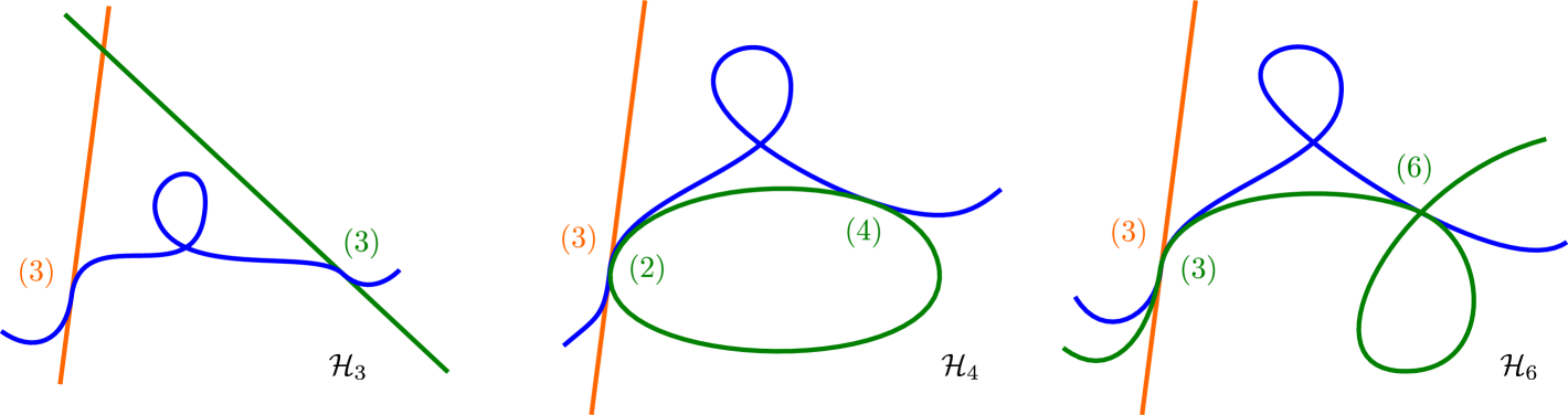
Figure 1. Configuration of the invariant curves for the foliations in Theorems 1, 2 and 3. In blue, the nodal cubics that produce the links; in orange, an inflectional line; in green, a line, a conic and a nodal cubic, respectively. Numbers denote local intersection multiplicities with the nodal cubic.

The planar models of Theorems 1, 2 and 3 (this is, both Pereira’s and our own) arise in a unified way through an unexpected connection with the Chazy equations. The latter appeared more than a hundred years ago in Chazy’s investigations on polynomial third-order equations which are free of movable critical points, investigations aimed at extending Painlevé’s work on second-order equations to higher order.

The reduced Chazy IV, V and VI equations are, respectively, the autonomous, third-order, ordinary differential equations

(4) $$x^{\prime\prime\prime} =3xx^{\prime\prime}+3(x^{\prime})^{2}-3x^{2}x^{\prime},$$

(5) $$x^{\prime\prime\prime} =2xx^{\prime\prime}+4(x^{\prime})^{2}-2x^{2}x^{\prime},$$

(6) $$x^{\prime\prime\prime} =xx^{\prime\prime}+5(x^{\prime})^{2}-x^{2}x^{\prime}$$

(see [Cha11, p. 336]; for their integration, see [Cha11, p. 343], [Cos00, Sections 6.4–6.6], or [Gui12]). These equations have the form $x^{\prime\prime\prime}=P(x,x^{\prime},x^{\prime\prime})$, with $P(x,y,z)$ a polynomial which is of degree $4$ when $x$, $y$ and $z$ are, respectively, given the weights $1$, $2$ and $3$. They may be described by polynomial vector fields on $\mathbb{C}^{3}$ of the form

$$W=y\frac{\partial}{\partial x}+z\frac{\partial}{\partial y}+P(x,y,z)\frac{\partial}{\partial z}.$$

The action of $\mathbb{C}^{*}$ on $\mathbb{C}^{3}$ associated to the above weights is given, for $\lambda\in\mathbb{C}^{*}$, by

(7) $$(x,y,z)\mapsto(\lambda x,\lambda^{2}y,\lambda^{3}z).$$

The previous quasihomogeneity property for $P$ is equivalent to the fact that $P(\lambda x,\lambda^{2}y,\lambda^{3}z)=\lambda^{4}P(x,y,z)$. The transformation (7) acts upon a vector field $W$ as above by dividing it by $\lambda$. The action preserves thus the foliation on $\mathbb{C}^{3}$ induced by $W$, and induces a foliation on the quotient of $\mathbb{C}^{3}\setminus\{0\}$ under the above action, the two-dimensional variety known as the weighted projective plane $\mathbb{P}(1,2,3)$ (to be discussed in Section 2.3).

Theorem 4.

The foliations on $\mathbb{P}(1,2,3)$ induced by the reduced Chazy IV, V and VI equations are birationally equivalent to the foliations $\mathcal{F}_{3}$, $\mathcal{F}_{4}$ and $\mathcal{F}_{6}$, respectively.

Brunella considered that “it would be natural to look for other types of birational models [for $\mathcal{F}_{3}$]” [Bru15, p. 54]. The above result provides alternative models, not just for $\mathcal{F}_{3}$, but for $\mathcal{F}_{4}$ and $\mathcal{F}_{6}$ as well. It will follow, on the one hand, from the definitions of these foliations as quotients, and, on the other, from the description of the foliations induced by the corresponding Chazy equations appearing in [Gui12, pp. 71–74]. We will revisit this last result in Section 4. Theorems 2 and 3, and an alternative proof of Theorem 1, will follow from it, and from an explicit birational equivalence between $\mathbb{P}(1,2,3)$ and $\mathbb{P}^{2}$.

The foliation $\mathcal{F}_{3}$ has a characterizing involution, the foliated flop (see Section 3), central to Brunella’s interest in it [Bru99]. We can fully describe the groups of birational automorphisms of all of these foliations.

Theorem 5.

The groups of birational automorphisms are:

1. for $\mathcal{F}_{3}$, a group of order six, isomorphic to the group of permutations in three symbols $S_{3}$;

2. for $\mathcal{F}_{4}$, a group of order two (generated by an involution); and

3. for $\mathcal{F}_{6}$, trivial.

For the models for $\mathcal{F}_{3}$ and $\mathcal{F}_{4}$ given in Theorems 1 and 2, Propositions 13 and 15 will give explicit formulas for generators of these groups.

The connection between the special quotient foliations and the Chazy equations will also bear fruits on the Chazy side. The symmetries of the quotient foliations will allow us, from a solution to either the reduced Chazy IV or V equation, to produce another solution of the same equation. This is the content of the next two results.

Theorem 6.

If $x(t)$ is a solution to the reduced Chazy IV equation (4), so are

(8) $$\frac{2xx^{\prime}-x^{\prime\prime}}{x^{\prime}},$$

(9) $$\frac{x^{2}-x^{\prime}}{x},$$

$$\frac{x^{3}-3xx^{\prime}+x^{\prime\prime}}{x^{2}-x^{\prime}},\;\;-\frac{x^{\prime}(x^{3}-3xx^{\prime}+x^{\prime\prime})}{x^{2}x^{\prime}+(x^{\prime})^{2}-xx^{\prime\prime}},\text{ and }\;\frac{x^{2}x^{\prime}-xx^{\prime\prime}+(x^{\prime})^{2}}{2xx^{\prime}-x^{\prime\prime}}.$$

The first transformation is involutive, the second of order three, and these two generate a group isomorphic to $S_{3}$, which contains the other three substitutions.

Theorem 7.

If $x(t)$ is a solution to the reduced Chazy V equation (5), so is

$$\frac{x^{3}-3xx^{\prime}+x^{\prime\prime}}{x^{2}-x^{\prime}}.$$

This transformation is involutive.

The foliation $\mathcal{F}_{6}$ may be obtained as a quotient of $\mathcal{F}_{3}$ (this will be explained in Section 3.3). This fact, together with Theorem 4, will be the basis of a relation between the solutions of the associated Chazy equations:

Theorem 8.

Let $x(t)$ be a solution to the reduced Chazy IV equation (4). Then

$$\frac{xx^{\prime\prime}-2(x^{\prime})^{2}}{x^{\prime\prime}-xx^{\prime}}$$

is a solution to the reduced Chazy VI equation (6), and every solution to the latter may be obtained in this form. The solution to the reduced Chazy VI equation obtained from $x(t)$ coincides with the solution obtained from (8).

The models of Theorems 1, 2 and 3 are all degree-two foliations, and, in this sense, have minimal complexity among all possible birational models on $\mathbb{P}^{2}$ for the corresponding foliations. In the next result, we present another degree-two planar model for $\mathcal{F}_{3}$, not linearly equivalent to that of Theorem 7, in which all the singularities are non-degenerate, and for which its birational automorphisms of order three are linear—they are cubic in Pereira’s model (1). In this model, Brunella’s flop is represented by a de Jonquières involution of degree four.

Theorem 9.

Brunella’s very special foliation $\mathcal{F}_{3}$ can be represented in $\mathbb{P}^{2}$ as the degree-two foliation $\mathcal{J}$ defined by the vanishing of

(10) $$\Omega=yz(x+y-2z)\,\mathrm{d}x+xz(y+z-2x)\,\mathrm{d}y+xy(z+x-2y)\,\mathrm{d}z.$$

Its set of invariant algebraic curves is composed by the nodal cubic $xy^{2}+yz^{2}+zx^{2}-3xyz=0$, representing the link, and by the three coordinate lines, tangent to the latter. It is the only degree-two foliation of $\mathbb{P}^{2}$ leaving invariant this configuration of curves. Its group of birational automorphisms is generated by the quartic de Jonquières involution

(11) $$J_{4}(x:y:z)=(y(y-z)(z-x)^{2}:x(x-y)(y-z)^{2}:z(z-x)(x-y)^{2}),$$

and by the cyclic permutation of the coordinates.

We will present a complete factorization of $J_{4}$ as a composition of three standard quadratic Cremona transformations in Section 5.2.

The foliations $\mathcal{F}_{3}$, $\mathcal{F}_{4}$ and $\mathcal{F}_{6}$ can be characterized as quotients of linear foliations on $\mathbb{P}^{2}$ under the action of non-involutive monomial birational transformations (see Section 7). Involutive cases are given by the action of the standard quadratic Cremona involution, and we investigate this in Section 6. We begin by studying the quotient of the plane by the standard Cremona involution, which is identified to Cayley’s nodal cubic surface, and which is birationally equivalent to the plane (a singular del Pezzo surface). As a by-product of this analysis, we obtain the following result:

Theorem 10.

Let $\lambda\in\mathbb{C}\setminus\{0,1\}$. The quotient of the degree-one foliation on $\mathbb{P}^{2}$ given by $\lambda YZ\,\mathrm{d}X-XZ\,\mathrm{d}Y+(1-\lambda)XY\,\mathrm{d}Z=0$, under the action of the standard quadratic Cremona transformation $(X:Y:Z)\mapsto(YZ:ZX:XY)$, is birationally equivalent to the foliation $\mathcal{G}_{\lambda}$ of degree three on $\mathbb{P}^{2}$ given by

(12) $${y}{z}({y}+{z})\left\{(\lambda+1){x}+{y}+\lambda{z}\right\}\,\mathrm{d}{x}-{x}{z}({x}+{z})\left\{(\lambda-1){x}+(2\lambda-1){y}+\lambda{z}\right\}\,\mathrm{d}{y}+\\ +{x}{y}({x}+{y})\left\{(\lambda-1){x}-{y}+(\lambda-2){z}\right\}\,\mathrm{d}{z}=0.$$

The article is organized in the following way. After reviewing some background material in Section 2, we recall the definition of the three special quotient foliations in Section 3. In Section 4 we study the relations between the Chazy equations and the special quotient foliations, and establish Theorem 4. This will allow us to give an alternative proof of Theorem 1 in Section 4.1.1, and to prove Theorems 2 and 3 in Sections 4.2.1 and 4.3.1, respectively. Theorems 6, 7 and 8 will be established in the same section. Section 5 will be devoted to Theorem 9, and Theorem 10 will proved in Section 6. Theorem 5, whose proof is more analytic in nature, will be established in Section 7, where we will also calculate the groups of birational automorphisms of hyperbolic linear foliations of the plane (Theorem 17).

Acknowledgments

The authors thank the kind attentions of Vitalino Cesca Filho, Charles Favre, Frank Loray, Iván Pan, and Edileno dos Santos. And last, but not least, thanks to Pedro Fortuny Ayuso, whose Maple code for reduction of singularities was very useful.

2. Background material on singularities of foliations and surfaces

2.1. On singular holomorphic foliations

We refer the reader to the first chapters of [Bru15] for a detailed exposition of what follows. A singular holomorphic foliation of a smooth surface $M$ can be given by a locally finite open covering $\{U_{i}\}$ and local differential equations given by the vanishing of

$$\omega_{i}=a_{i}(x_{i},y_{i})\,\mathrm{d}x_{i}+b_{i}(x_{i},y_{i})\,\mathrm{d}y_{i},$$

where $a_{i},b_{i}\in\mathcal{O}(U_{i})$, with $\gcd(a_{i},b_{i})=1$, such that, along $U_{i}\cap U_{j}\neq\emptyset$, $\omega_{i}=g_{ij}\,\omega_{i}$ for $g_{ij}\in\mathcal{O}^{*}(U_{i}\cap U_{j})$. The singularities of the foliation are given by the zeros of the forms $\omega_{i}$. The conditions $\gcd(a_{i},b_{i})=1$ ensure that the singular set is locally finite. The foliation locally defined by the $1$-form $\omega=a(x,y)\,\mathrm{d}x+b(x,y)\,\mathrm{d}y$ may also be defined by its dual vector field $v=b(x,y)\,\partial/\partial x-a(x,y)\,\partial/\partial y$. A singular point of the foliation, a point where both $a$ and $b$ vanish, is said to be non-degenerate if the eigenvalues of the linear part of $v$ at this singular point are both non-zero. In such a case, if $\lambda_{1}$ and $\lambda_{2}$ are these eigenvalues, the eigenvalues of the singular point are said to be $\lambda_{2}:\lambda_{1}$ (or $\lambda_{1}:\lambda_{2}$). A singularity $p$ of the foliation is said to be reduced if $v$ has a non-nilpotent linear part at $p$, and if it has either one vanishing eigenvalue, or it is non-degenerate and $\lambda_{2}/\lambda_{1}\not\in\mathbb{Q}^{+}$. After a finite number of blow-ups, every singularity of a foliation is replaced by finitely many reduced singularities along the exceptional divisor (Seidenberg’s reduction of singularities).

The non-degenerate singularities of eigenvalues $n:1$, with $n$ a strictly positive integer, admit the local Poincaré-Dulac normal form, $(ny+\epsilon x^{n})\,\mathrm{d}x-x\,\mathrm{d}y$, with $\epsilon\in\{0,1\}$, for which the curve $x=0$ is invariant. For $\epsilon=1$, this is the only invariant curve. In particular, if there is more than one invariant curve through such a singularity, it is linearizable (has $\epsilon=0$ in its normal form). For $\epsilon=0$, we have the first integral $y/x^{n}$, and, with it, the invariant curves of the form $y=cx^{n}$, any two of which have a contact of order $n$. When $n>1$, blowing up the foliation $ny\,\mathrm{d}x-x\,\mathrm{d}y$ produces an invariant divisor with two singularities, one of type $n:1-n$, and one of type $n-1:1$, a linearizable one. Blowing up the radial foliation $y\,\mathrm{d}x-x\,\mathrm{d}y$ (the above foliation in the case $n=1$) produces a dicritical exceptional divisor, one that is everywhere transverse to the foliation.

Let $\nu(p)\geq 0$ be the order of the first non-trivial jet of a $1$-form $\omega=a(x,y)\,\mathrm{d}x+b(x,y)\,\mathrm{d}y$ defining a local foliation $\mathcal{F}$ around $p$; define $l(p,\mathcal{F}):=\nu(p)$ if $p$ is not dicritical and $l(p,\mathcal{F}):=\nu(p)+1$ if $p$ is dicritical. For example, for a reduced singular point, $\nu(p)=l(p,\mathcal{F})=1$, and for a radial point, $\nu(p)=1$ and $l(\mathcal{F},p)=2$.

The multiplicity (or Milnor number) $\mu(p,\mathcal{F})$ of a singularity $p$ of the foliation $\mathcal{F}$ given by $a(x,y)\,\mathrm{d}x+b(x,y)\,\mathrm{d}y=0$ is the intersection multiplicity of the curves $a(x,y)=0$ and $b(x,y)=0$ at $p$. The Milnor number of a non-dicritical singularity can be computed in terms of $l(p,\mathcal{F})$ and the sum of Milnor numbers of the transformed foliation $\overline{\mathcal{F}}$ by a blow-up $\sigma$ at $p$ along $E=\sigma^{-1}(p)$ (see [Bru15] p. 5):

(13) $$\mu(p,\mathcal{F})=l(p,\mathcal{F})(l(p,\mathcal{F})-1)-1+\sum_{q\in E}\mu(q,\overline{\mathcal{F}}).$$

For a singular holomorphic foliation of $\mathbb{P}^{2}$, its degree is the number of tangencies of a generic leaf of $\mathcal{F}$ and a generic projective line.

Proposition 11 (Darboux’s formula).

For a singular holomorphic foliation $\mathcal{F}$ of $\mathbb{P}^{2}$ (with finite singular set),

$$\deg^{2}(\mathcal{F})+\deg(\mathcal{F})+1=\sum_{p\in\mathrm{sing}(\mathcal{F})}\mu(p,\mathcal{F}).$$

The next proposition (see [MP05, Lemma 1], or [ACFLl21, Lemma 16]), will be used for understanding the effect on foliations of the building blocks of Cremona maps:

Proposition 12.

Let $Q(x:y:z)=(yz:xz:xy)$ be the standard quadratic Cremona map. Let $p_{1}$, $p_{2}$ and $p_{3}$ be the vertices of the coordinate triangle $xyz=0$. Let $\mathcal{F}$ be a foliation of the plane of degree $\deg(\mathcal{F})$, with $l(p_{i},\mathcal{F})\geq 0$. Let $\overline{\mathcal{F}}$ be the transformed foliation of $\mathcal{F}$ under $Q$ (with finite singular set). Then,

$$\deg(\overline{\mathcal{F}}) =2\deg(\mathcal{F})+2-\sum_{i=1}^{3}l(p_{i},\mathcal{F}),$$

$$l(p_{i},\overline{\mathcal{F}}) =\deg(\mathcal{F})+2-l(p_{j},\mathcal{F})-l(p_{k},\mathcal{F}),\quad i\neq j\neq k.$$

A foliation on $\mathbb{P}^{2}$ of degree $d$ may be given by a polynomial homogeneous vector field on $\mathbb{C}^{3}$ of degree $d$, or by a homogeneous polynomial $1$-form $\Omega$ on $\mathbb{C}^{3}$, of degree $d+1$ such that, for the Euler vector field $E=x\,\partial/\partial x+y\,\partial/\partial y+z\,\partial/\partial z$, $\Omega(E)=0$; this is, if $\Omega=A\,\mathrm{d}x+B\,\mathrm{d}y+C\,\mathrm{d}z$, the relation $xA+yB+zC=0$ holds. Every such polynomial homogeneous $1$-form $\Omega$ satisfies the Frobenius integrability condition $\Omega\wedge\mathrm{d}\Omega=0$.

For a curve $C$ in $\mathbb{P}^{2}$ defined by the homogeneous polynomial $g$, and a foliation on $\mathbb{P}^{2}$ defined by the homogeneous $1$-form $\Omega$ on $\mathbb{C}^{3}$, $C$ will be invariant by the foliation if and only if there exists a homogeneous $2$-form $\Theta$ such that $\mathrm{d}g\wedge\Omega=g\Theta$. For a given homogeneous polynomial $g$, the above condition on the space of homogeneous $1$-forms $\Omega$ of a given degree is a linear one.

2.2. The Klein surface singularities of type $A_{n}$

We follow [dlHS79, Section IV] for the discussion that follows. Let $n\geq 1$. Consider the analytic space

$$A_{n}=\{(x,y,z)\in\mathbb{C}^{3}\mid z^{n+1}=xy\}.$$

Let $C_{n+1}\subset\mathrm{GL}(2,\mathbb{C})$ be the subgroup generated by $(s,t)\mapsto(\beta^{-1}s,\beta t)$, with $\beta$ a primitive $(n+1)$-th root of unity. Let $X_{n+1}=\mathbb{C}^{2}/C_{n+1}$. The injective analytic map $\phi_{n+1}:X_{n+1}\to A_{n}$ given by $\phi_{n+1}(s,t)=(s^{n+1},t^{n+1},st)$, realizes an analytic equivalence between $X_{n+1}/C_{n+1}$ and $A_{n}$.

For the desingularization of $A_{n}$, consider $n+1$ copies $R_{0},\ldots,R_{n}$ of $\mathbb{C}^{2}$, with coordinates $(u_{i},v_{i})$ on $R_{i}$, glued by the functions $\varphi_{k-1}:R_{k-1}\dashrightarrow R_{k}$ given by

$$(u_{k},v_{k})=\varphi_{k-1}(u_{k-1},v_{k-1})=(u_{k-1}^{2}v_{k-1},u_{k-1}^{-1}),$$

for $k=1,\ldots,n$. This gluing defines a manifold $M_{n}$, and the mappings $\rho_{k}:R_{k}\to A_{n}$,

$$\rho_{k}(u_{k},v_{k})=(u_{k}^{n-k+1}v_{k}^{n-k},u_{k}^{k}v_{k}^{k+1},u_{k}v_{k}),$$

define a global map $\rho:M_{n}\to A_{n}$, the resolution of $A_{n}$.

The exceptional divisor of $\rho$ is a chain of $n$ smooth compact rational curves $C_{1},\ldots,C_{n}$, with $C_{i}^{2}=-2$, where $C_{i}$ intersects $C_{i+1}$ transversely at one point, and $C_{i}\cap C_{j}=\emptyset$ if $|i-j|\geq 2$. This combinatorics characterizes $A_{n}$, in the sense that the contraction of a chain of rational curves in a surface having it is analytically equivalent to $A_{n}$ [BHPV04, Thm. 5.1, Ch. III].

Holomorphic actions of finite groups are holomorphically linearizable in a neighborhood a fixed point, and thus $A_{n}$ gives the local model for the quotient of the action of $\mathbb{Z}_{n+1}$ generated by a transformation that, at a fixed point, has eigenvalues $\beta$ and $\beta^{n}$ [BHPV04, Thm. 5.4, Ch. III].

2.3. A weighted projective plane and the standard one

The quotient of $\mathbb{C}^{3}\setminus\{0\}$ under the action of the weighted homotheties (7) is the weighted projective plane $\mathbb{P}(1,2,3)$. The class of $(x,y,z)\in\mathbb{C}^{3}\setminus\{0\}$ in $\mathbb{P}(1,2,3)$ will be denoted by $[x:y:z]$. The weighted projective plane $\mathbb{P}(1,2,3)$ is covered by three charts, each one of which is either $\mathbb{C}^{2}$, or its quotient under the action of a finite linear group:

• the chart $(y,z)\mapsto[1:y:z]$ is injective;

• the chart $(x,z)\mapsto[x:1:z]$ is injective up to the action of $(x,z)\mapsto(-x,-z)$;

• the chart $(x,y)\mapsto[x:y:1]$ is injective up to the action of $(x,y)\mapsto(\omega x,\omega^{2}y)$, with $\omega$ a primitive cubic root of unity.

The plane $\mathbb{P}(1,2,3)$ is thus a normal analytic space, with two singular points: $p_{1}=[0:1:0]$, of type $A_{1}$, and $p_{2}=[0:0:1]$, of type $A_{2}$. It is birationally equivalent to $\mathbb{P}^{2}$: the identification between affine charts $j([1:y:z])=(1:y:z)$, given in quasihomogeneous coordinates, for $x\neq 0$, by

$$j([x:y:z])=j\left(\left[1:\frac{y}{x^{2}},\frac{z}{x^{3}}\right]\right)=\left(1:\frac{y}{x^{2}},\frac{z}{x^{3}}\right)=(x^{3}:xy:x^{2}z),$$

extends to the birational map $j:\mathbb{P}(1,2,3)\dashrightarrow\mathbb{P}^{2}$

(14) $$[x:y:z]\mapsto(x^{3}:xy:z),$$

having inverse $(X:Y:Z)\mapsto[X:XY:X^{2}Z]$. A factorization of this birational map is given as follows. Consider the resolution $\pi:S\to\mathbb{P}(1,2,3)$ of $\mathbb{P}(1,2,3)$, obtained by desingularizing the $A_{1}$ and $A_{2}$ singular points, as explained in Section 2.2. The surface $S$ has a $(-2)$-curve $C_{1}$ (i.e. a smooth rational curve of self-intersection $-2$), corresponding to the resolution of $A_{1}$, and a chain of two $(-2)$-curves, $D_{1}$ and $D_{2}$, intersecting transversely at one point, corresponding to the resolution of $A_{2}$. The strict transform of the curve $\mathcal{\ell}$ given by $x=0$ is a rational curve $\overline{\ell}$ in $S$ of self-intersection $-1$, intersecting $C_{1}$ and $D_{1}$ at one point each, transversely. The contractions of $\overline{\ell}$ and the transforms of $D_{1}$ and $D_{2}$, in this order, produce the projective plane, where the transform of $C_{1}$ is a straight line. See Figure 2.

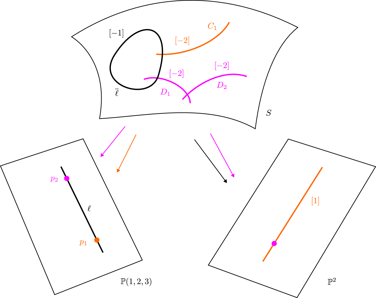
Figure 2. Birational equivalence between $\mathbb{P}(1,2,3)$ and $\mathbb{P}^{2}$. Numbers in square brackets denote the self-intersection of the corresponding curve.

3. Three special quotient foliations

For $n\in\{3,4,6\}$, the foliation $\mathcal{F}_{n}$ admits a simple description as quotient of a foliation on a rational surface under the action of a cyclic group of automorphisms of order $n$. This surface has an invariant cycle of rational curves $\Delta_{n}$ of length $n$, whose components are cyclically permuted by the automorphism, and which produces the link in the quotient. This is schematically presented in Figure 3. We now present these foliations and exhibit some of their birational symmetries (Theorem 5 will establish that there are no further ones).

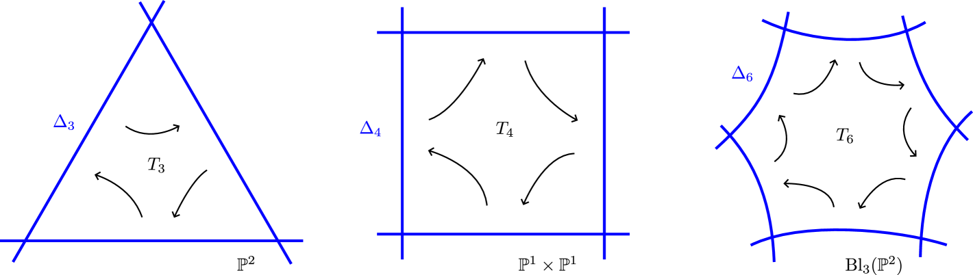
Figure 3. The cycles of rational curves and the effect on them of the automorphisms of order three, four and six, respectively.

3.1. Brunella’s very special foliation, $\mathcal{F}_{3}$

The foliation and its characterizing birational involution first appeared in [Bru99]; it is discussed in detail in [Bru15, Ch. 4, Sect. 2]. Let $\omega$ be a primitive cubic root of unity. Consider the degree-one foliation $\mathcal{E}_{3}$ on $\mathbb{P}^{2}$ given by

(15) $$\omega^{2}YZ\,\mathrm{d}X+\omega XZ\,\mathrm{d}Y+XY\,\mathrm{d}Z=0.$$

It is tangent to the coordinate triangle $\Delta_{3}:XZY=0$, and has three reduced non-degenerate singular points at its vertices. It is preserved by the linear automorphism of order three

(16) $$T_{3}(X:Y:Z)=(Z:X:Y).$$

The action of $T_{3}$ on $\mathbb{P}^{2}$ is not free, and the quotient $\mathbb{P}^{2}/T_{3}$ is a singular variety. The automorphism $T_{3}$ has the three fixed points $(1:1:1)$, $(1:\omega:\omega^{2})$ and $(1:\omega^{2}:\omega)$. At each one of them, the linear part of its derivative has eigenvalues $\omega$ and $\omega^{2}$, and the quotient $\mathbb{P}^{2}/T_{3}$ has three singular points of type $A_{2}$. Consider the minimal desingularization $M_{3}\to\mathbb{P}^{2}/T_{3}$, defined on the rational surface $M_{3}$. The foliation $\mathcal{F}_{3}$, which we will call Brunella’s very special foliation, is the foliation on $M_{3}$ induced by $\mathcal{E}_{3}$. It has a link $C$ (in the sense of Section 1), image of $\Delta_{3}$, with $C^{2}=3$.

Both the birational involution of $\mathbb{P}^{2}$ given by the standard quadratic Cremona transformation

(17) $$Q(X:Y:Z)=(YZ:ZX:XY),$$

and the linear symmetry of order three

(18) $$S(X:Y:Z)=(X:\omega Y:\omega^{2}Z),$$

preserve the foliation $\mathcal{E}_{3}$, and commute with $T_{3}$. They induce birational symmetries of $\mathcal{F}_{3}$ on $\mathbb{P}^{2}/T_{3}$, and, since $Q\circ S\circ Q=S^{-1}$, they generate a group of birational automorphisms of $\mathcal{F}_{3}$, of order six, isomorphic to the group of permutations in three symbols $S_{3}$ (Theorem 5 will establish that these are all of its birational automorphisms).

The birational involution of $\mathcal{F}_{3}$ associated to the Cremona involution (17) will be called Brunella’s foliated flop. It can be factored as follows:

• first, a blow-up $\sigma$ of the node $p$ of the link $C$ transforms it into a curve $\overline{C}$ of self-intersection $-1$;

• then, the contraction of $\overline{C}$ transforms the exceptional divisor $\sigma^{-1}(p)$ into a rational curve with a node, of self-intersection $3$, which becomes the new link.

This is schematically presented in Figure 4.

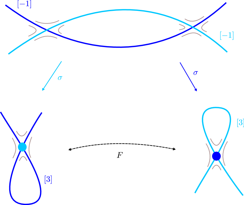
Figure 4. Brunella’s foliated flop and its factorization.

3.2. Santos’s foliation $\mathcal{F}_{4}$

Consider the foliation $\mathcal{E}_{4}$ on $\mathbb{P}^{1}\times\mathbb{P}^{1}$ given in the affine chart $(X:1,Y:1)$ by

(19) $$Y\,\mathrm{d}X-\mathrm{i}X\,\mathrm{d}Y=0,$$

for $\mathrm{i}=\sqrt{-1}$. It is tangent to the cycle $\Delta_{4}$ of four lines formed by $\mathbb{P}^{1}\times\{0\}$, $\mathbb{P}^{1}\times\{\infty\},$ $\{0\}\times{\mathbb{P}}^{1}$, and $\{\infty\}\times\mathbb{P}^{1}$, and has reduced non-degenerate singularities at its vertices. The order-four automorphism $T_{4}$ of $\mathbb{P}^{1}\times\mathbb{P}^{1}$

(20) $$T_{4}(X:1,Y:1)=(Y:1,1:X)$$

permutes cyclically the four lines of $\Delta_{4}$, and preserves the foliation $\mathcal{E}_{4}$. It acts freely in a neighborhood of $\Delta_{4}$. The transformation $T_{4}$ has two fixed points, $(1:1,1:1)$ and $(-1:1,-1:1)$, at which the eigenvalues of the derivative of $T_{4}$ are $\mathrm{i}$ and $-\mathrm{i}$. It also has an orbit of length two, formed by $(-1:1,1:1)$ and $(1:1,-1:1)$, at which the derivative of $T^{2}$ has twice the eigenvalue $-1$. The variety $(\mathbb{P}^{1}\times\mathbb{P}^{1})/T_{4}$ has four singular points, two of type $A_{3}$ and one of type $A_{1}$. The minimal desingularization $M_{4}\to(\mathbb{P}^{1}\times\mathbb{P}^{1})/T_{4}$ is endowed with a foliation, Santos’s foliation $\mathcal{F}_{4}$, coming from $\mathcal{E}_{4}$, and a link $C$ (in the sense of Section 1), image of $\Delta_{4}$, with $C^{2}=2$ (see [San17]).

The linear involution $J:(\mathbb{P}^{1}\times\mathbb{P}^{1})\to(\mathbb{P}^{1}\times\mathbb{P}^{1})$,

(21) $$J(X:1,Y:1)=(-X:1,-Y:1)$$

preserves the form (19) and commutes with $T_{4}$: it induces a birational involution of $M_{4}$ that preserves $\mathcal{F}_{4}$ (Theorem 5 will show that this is its only non-trivial birational automorphism).

3.3. Santos’s foliation $\mathcal{F}_{6}$

Let us consider again the foliation $\mathcal{E}_{3}$ of $\mathbb{P}^{2}$ of Section 3.1 of Eq. (15). Let $\sigma:\mathrm{Bl}_{3}(\mathbb{P}^{2})\to\mathbb{P}^{2}$ be the composition of the blowing-ups at the vertices $(0:0:1)$, $(0:1:0)$, and $(1:0:0)$. Consider the cycle $\Delta_{6}$ of six $(-1)$-curves on $\mathrm{Bl}_{3}(\mathbb{P}^{2})$ composed by the transformed of the coordinate triangle of $\mathbb{P}^{2}$ by $\sigma$, and by the three exceptional lines of $Q$. Denote by $\mathcal{E}_{6}$ the transformed foliation of $\mathcal{E}_{3}$ by $Q$; it is tangent to $\Delta_{6}$, and has reduced non-degenerate singularities at its six vertices. The linear transformation $T_{3}$ of $\mathbb{P}^{2}$ of Eq. (16) commutes with the Cremona involution $Q$ in Eq. (17), and $T_{3}\circ Q$ is a birational automorphism of order six of $\mathbb{P}^{2}$ preserving $\mathcal{L}$. It induces a biholomorphism $T_{6}$ of $\mathrm{Bl}_{3}(\mathbb{P}^{2})$, which permutes cyclically the six rational curves of $\Delta_{6}$, and preserves the foliation $\mathcal{E}_{6}$. The automorphism $T_{6}$ has a fixed point coming from $(1:1:1)$, the common fixed point of $T_{3}$ and $Q$; an orbit of order two coming from the other fixed points of $T_{3}$, $(1:\omega:\omega^{2})$ and $(1:\omega^{2}:\omega)$; and an orbit of order three, formed by the other fixed points of $Q$, $(1:1:-1)$, $(-1:1:1)$ and $(1:-1:1)$. The quotient $\mathrm{Bl}_{3}(\mathbb{P}^{2})/T_{6}$ has three singular points, which turn out to be of types $A_{5}$, $A_{2}$ and $A_{1}$. On the minimal desingularization $M_{6}\to\mathrm{Bl}_{3}(\mathbb{P}^{2})/T_{6}$, we have a foliation induced by $\mathcal{E}_{6}$. This is Santos’s foliation $\mathcal{F}_{6}$. It has a link $C$ (in the sense of Section 1), image of $\Delta_{6}$, with $C^{2}=1$ (see [San17]).

Observe that, by construction, Santos’s foliation $\mathcal{F}_{6}$ is birationally equivalent to the quotient of $\mathcal{F}_{3}$ under the action of Brunella’s foliated flop.

4. Chazy equations and foliations on a weighted projective plane

4.1. Chazy IV and $\mathcal{G}_{\mathrm{IV}}$

We begin by describing the relation between the reduced Chazy IV equation and Brunella’s very special foliation following [Gui12]. The Chazy IV equation (4) is given by the vector field

$$W=y\frac{\partial}{\partial x}+z\frac{\partial}{\partial y}+3(xz+y^{2}-x^{2}y)\frac{\partial}{\partial z},$$

which induces the foliation on $\mathbb{P}(1,2,3)$ that will be denoted by $\mathcal{G}_{\mathrm{IV}}$. The latter may also be defined by the quasihomogeneous form

(22) $$3(2x^{2}y^{2}-2xyz-2y^{3}+z^{2})\,\mathrm{d}x-3(x^{2}-y)(xy-z)\,\mathrm{d}y+(2y^{2}-xz)\,\mathrm{d}z,$$

the form $i_{W}\circ i_{L}(\mathrm{d}x\wedge\mathrm{d}y\wedge\mathrm{d}z)$, with $L=x\,\partial/\partial x+2y\,\partial/\partial y+3z\,\partial/\partial z$ the vector field generating the weighted homotheties (7). (Here, $i_{Z}\eta$ denotes the contraction of the form $\eta$ by the vector field $Z$.)

The vector field $W$ has the quasihomogeneous first integral of degree three $B=x^{3}-3xy+z$, and the invariant surface given by the quasihomogeneous polynomial of degree six

$$C=3y^{2}x^{2}-y^{3}-3xyz+z^{2}.$$

Let $\Sigma=B^{-1}(1)$. The vector field $W$ is tangent to $\Sigma$, and induces on it a foliation, that we will denote by $\widetilde{\mathcal{G}}_{\mathrm{IV}}$. There is an action of $\mathbb{Z}_{3}$ on $\mathbb{C}^{3}$ given by the restriction of the weighted homotheties (7) to the group of cubic roots of unity. It preserves $\Sigma$ along with $\widetilde{\mathcal{G}}_{\mathrm{IV}}$. The quotient of $\Sigma$ under this action is realized by the restriction to $\Sigma$ of the quotient map $\pi:\mathbb{C}^{3}\setminus\{0\}\to\mathbb{P}(1,2,3)$. The image of $\Sigma$ is the complement of the curve $B=0$ in $\mathbb{P}(1,2,3)$, and the image of $\widetilde{\mathcal{G}}_{\mathrm{IV}}$ is the restriction of $\mathcal{G}_{\mathrm{IV}}$ to this image.

On the other hand, we have the foliation $\mathcal{E}_{3}$ on $\mathbb{P}^{2}$ described in Section 3.1. There is an action of $\mathbb{Z}_{3}$ on $\mathbb{P}^{2}$ preserving $\mathcal{E}_{3}$, given by the transformation $T_{3}$ of Eq. (16); the quotient of $\mathbb{P}^{2}$ is a rational surface, and the induced foliation is Brunella’s very special foliation $\mathcal{F}_{3}$.

We will exhibit a birational map $\Phi_{3}:\mathbb{P}^{2}\dashrightarrow\Sigma$ that maps $\mathcal{E}_{3}$ to $\widetilde{\mathcal{G}}_{\mathrm{IV}}$, and that is equivariant with respect to the actions of $\mathbb{Z}_{3}$. This will establish the relation between $\mathcal{F}_{3}$ and $\mathcal{G}_{\mathrm{IV}}$ announced in Theorem 4.

Consider the linear vector field $D_{3}$ on $\mathbb{P}^{2}$ that in the affine chart $(X:Y:1)$ reads

(23) $$(\omega-1)\left(X\frac{\partial}{\partial X}-\omega Y\frac{\partial}{\partial Y}\right),$$

and which is tangent to the foliation $\mathcal{E}_{3}$ of Eq. (15). Consider the rational function on $\mathbb{P}^{2}$

$$f=-\frac{(\omega+1)(\omega^{2}Y+\omega X+1)}{\omega^{2}Y+X+\omega}.$$

A straightforward calculation shows that, with respect to the derivation given by $D_{3}$, $f$ is a solution to the reduced Chazy IV equation (4). (The above expression for $f$ corrects the one given in [Gui12, p. 72].)

The map $\mathbb{P}^{2}\dashrightarrow\mathbb{C}^{3}$, given by $(X:Y:1)\mapsto(f,D_{3}f,D_{3}^{2}f)$ takes values in $\Sigma$ and defines a map $\Phi_{3}:\mathbb{P}^{2}\dashrightarrow\Sigma$. Since $f$ satisfies the Chazy IV equation with respect to the derivation given by $D_{3}$, $\Phi_{3}$ maps $D_{3}$ to the restriction of $W$ to $\Sigma$, thus mapping $\mathcal{E}_{3}$ to $\widetilde{\mathcal{G}}_{\mathrm{IV}}$. The map $\Phi_{3}$ is equivariant with respect to the action of $\mathbb{Z}_{3}$ on $\mathbb{P}^{2}$ given by the transformation $T_{3}$ of Eq. (16), and to its previously described action on $\Sigma$. It is a birational one, for its inverse, when $\Sigma$ is parametrized by $(x,y)\mapsto(x,y,1-x^{3}+3xy)$, is given by

$$(x,y)\mapsto\left(x^{2}+x-y+1:x^{2}+\omega^{2}x-y+\omega:x^{2}+\omega x-y+\omega^{2}\right).$$

In this way, Brunella’s very special foliation, given by the quotient of the foliation on $\mathbb{P}^{2}$ induced by $D_{3}$ under the action of $\mathbb{Z}_{3}$ given by Eq. (16), is birationally equivalent to the quotient of the foliation induced by $W$ on $\Sigma$, the foliation $\mathcal{G}_{\mathrm{IV}}$ on $\mathbb{P}(1,2,3)$ induced by the Chazy IV equation. Under this correspondence, the link corresponds to the curve defined by $C$.

Observe that, by developing $\Phi_{3}$, we obtain an explicit birational map from $\mathbb{P}^{2}$ to $\mathbb{P}(1,2,3)$ that realizes the quotient of $\mathbb{P}^{2}$ under the action of the cyclic permutation of variables (16), under which the pull-back of (22) is the form (15) defining the foliation $\mathcal{E}_{3}$ of Section 3.1.

Let us give explicit expressions in this model of $\mathcal{F}_{3}$ for the symmetries described in Section 3.1. We may conjugate the symmetries on $\mathbb{P}^{2}$ via $\Phi_{3}$, and obtain explicit birational transformations of $\Sigma$, which, on their turn, induce birational transformations of $\mathbb{P}(1,2,3)$ preserving $\mathcal{G}_{\mathrm{IV}}$. Brunella’s foliated flop, the symmetry associated to the Cremona involution (17), is the birational involution of $\mathbb{P}(1,2,3)$ given by

(24) $$[x:y:z]\mapsto[2xy-z:C:(3xy-2z)C];$$

the birational trivolution of $\mathbb{P}(1,2,3)$ induced by (18) is

(25) $$[x:y:z]\mapsto[x^{2}-y:x^{2}y-xz+y^{2}:3x^{4}y-2x^{3}z-3x^{2}y^{2}+3xyz-2y^{3}].$$

These two generate a group of birational transformations of $\mathbb{P}(1,2,3)$ preserving $\mathcal{G}_{\mathrm{IV}}$, isomorphic to the group, of order six, of permutations in three symbols $S_{3}$. This group can be promoted to a group of birational automorphisms of $\mathbb{C}^{3}$ that preserve the vector field associated to the reduced Chazy IV equation. This is the content of Theorem 6, which can be established by a direct calculation. In it, (8) corresponds to Brunella’s foliated flop, (9) to the above trivolution, and the remaining transformations to the other non-trivial elements of this group.

Let us analyze the invariant curves and the singularities of $\mathcal{G}_{\mathrm{IV}}$. For calculations in the smooth chart $[1:x:y]$ of $\mathbb{P}(1,2,3)$, biholomorphic to $\mathbb{C}^{2}$, one can simply restrict (22) to $\{x=1\}$. For calculations in the singular charts of $\mathbb{P}(1,2,3)$, one can resort to the formulas for the desingularizations of $A_{1}$ and $A_{2}$ discussed in Section 2.2. Both $B$ and $C$ give invariant curves for $\mathcal{G}_{\mathrm{IV}}$; we will denote them by the same symbols. The foliation $\mathcal{G}_{\mathrm{IV}}$ is regular at both $p_{1}$ and $p_{2}$, in the sense that, at each one of these points, it is the quotient of a regular foliation. In the smooth part of $\mathbb{P}(1,2,3)$, $\mathcal{G}_{\mathrm{IV}}$ has three non-degenerate singularities:

• $q_{1}=[1:0:0]$, with eigenvalues $-\omega:1$;

• $q_{2}=[1:1:2]$, a linearizable node with eigenvalues $1:3$;

• $q_{3}=[2:2:4]$, a saddle with eigenvalues $-3:2$.

The curve $C$ has two transverse smooth branches at $q_{1}$. The curves $B$ and $C$ are smooth and tangent at $q_{2}$, where they are tangent to the eigenvalue $1$. The curve $B$ passes also through $p_{1}$ and $q_{3}$. Since there are two smooth invariant curves through $q_{2}$ tangent to each other, the foliation is linearizable in a neighborhood of this singularity, and the curves have a contact of order $3$.

After desingularizing $p_{1}$ and $p_{2}$, and resolving the singularity of the foliation at $q_{2}$, we find three chains of two rational curves of self-intersection $-2$ each:

• one formed by the divisor in the desingularization of $p_{1}$, plus the strict transform of $B$;

• the divisor in the desingularization of $p_{2}$; and

• one formed by the invariant divisors in the resolution of $q_{2}$

(see the bottom left and the top of Figure 5). The contraction of each one of these chains gives a singularity of type $A_{2}$. These give the three singularities of the quotient model for $\mathcal{F}_{3}$. The link comes from the transform of $C$.

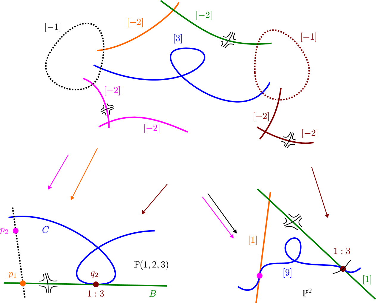
Figure 5. To the left, schematic minimal reduction of singularities of $\mathcal{G}_{\mathrm{IV}}$; to the right, a morphism to $\mathbb{P}^{2}$. Dotted lines represent curves that are not invariant by the foliation.

4.1.1. Birational equivalence between $\mathcal{G}_{\mathrm{IV}}$ and $\mathcal{F}_{3}$

Under the birational map (14), $\mathcal{G}_{\mathrm{IV}}$ induces the foliation of degree two on $\mathbb{P}^{2}$ given by (1), giving an alternative proof of Theorem 1. We remark that there is a full one-dimensional system (a pencil) of degree-two foliations leaving invariant the nodal cubic and the two inflectional tangents of Theorem 1, so, unlike the situation in Theorems 2 and Theorem 3, the foliation is not determined by its invariant algebraic curves.

By conjugating the birational symmetries (24) and (25) of $\mathcal{G}_{\mathrm{IV}}$ via the birational map (14), we obtain:

Proposition 13.

In homogeneous coordinates of $\mathbb{P}^{2}$, in the model (2) of $\mathcal{F}_{3}$, the birational involution induced by (17) is given by the quartic transformation

$$(x:y:z)\mapsto(x(2y-z)^{3}:(2y-z)\widetilde{C}:(3y-2z)\widetilde{C}),$$

for $\widetilde{C}=3xy^{2}-y^{3}-3xyz+xz^{2}$, and the birational trivolution induced by (16), by

$$(x:y:z)\mapsto((x-y)^{3}:(x-y)(xy-xz+y^{2}):3x^{2}y-2x^{2}z-3xy^{2}+3xyz-2y^{3}).$$

Let us describe the singularities of the foliation $\mathcal{H}_{3}$ on $\mathbb{P}^{2}$ given by (2). The singularities of $\mathcal{G}_{\mathrm{IV}}$ away from $\{x=0\}$ coming from $q_{1}$, $q_{2}$ and $q_{3}$, are respectively placed at $(1:0:0)$, $(1:1:2)$ and $(2:1:1)$, and admit the same local description. On the line $x=0$, we have the singular points $(0:1:3)$, a saddle with eigenvalues $-1:2$, and the point $(0:0:1)$, a nilpotent singularity with multiplicity three.

The composition of the resolution $\pi:S\to\mathbb{P}(1,2,3)$ with the map $j$ in (14) gives a resolution of this foliation of $\mathbb{P}^{2}$. See the right-hand side of Figure 5.

4.1.2. Relation with Pereira’s model

In [Per05, Sect. 5], Pereira gave a projective model for Brunella’s very special foliation $\mathcal{F}_{3}$. It is the degree-two foliation given by the vanishing of

(26) $$\Xi=Z(2XY-ZX-Y^{2})\,\mathrm{d}X-3XZ(X-Y)\,\mathrm{d}Y+X(ZX+XY-2Y^{2})\,\mathrm{d}Z.$$

It is tangent to the nodal cubic $Y^{3}+X^{2}Z+XZ^{2}-3XYZ=0$, and to its inflectional tangents $X=0$ and $Z=0$.

The foliation (1) is linearly equivalent to Pereira’s model for $\mathcal{F}_{3}$ (26), via the linear map $(x:y:z)=(X:X-Y:2X-3Y+Z)$, with inverse $(X:Y:Z)=(x:x-y:x-3y+z)$.

By conjugating by this map the birational symmetries of Proposition 13, we have:

Proposition 14.

Pereira’s model for the foliation $\mathcal{F}_{3}$, given by the vanishing of the form $\Xi$ of Eq. (26), is invariant by the quartic involutive Cremona map:

$$(X:Y:Z)\dashrightarrow(X(Y-Z)^{3}:(XZ-Y^{2})(Z-Y)(X-Y):(Y-X)^{3}Z),$$

and by the degree three Cremona trivolution $(X:Y:Z)\dashrightarrow(XZ^{2}:XYZ:Y^{3})$.

We observe that this trivolution type appears in [CD13, Prop. 6.23].

4.2. Chazy V and $\mathcal{G}_{\mathrm{V}}$

The associated vector field $W$ on $\mathbb{C}^{3}$ has the quasihomogeneous first integral of degree four $B=x^{4}-4x^{2}y+2zx-y^{2}$, and the invariant surface given by the quasihomogeneous polynomial of degree six

$$C=2y^{2}x^{2}-2xyz+z^{2}-2y^{3}.$$

Let $\Sigma=B^{-1}(1)$. It has a natural action of $\mathbb{Z}_{4}$ preserving the foliation induced by $W$, given by the restriction of (7) to the group of fourth roots of unity.

Let $D_{4}$ be the vector field on $\mathbb{P}^{1}\times\mathbb{P}^{1}$ that, in the chart $(X:1,Y:1)$, reads

$$(\mathrm{i}-1)\left(\mathrm{i}X\frac{\partial}{\partial X}+Y\frac{\partial}{\partial Y}\right),$$

and which is tangent to the foliation $\mathcal{E}_{4}$ of Eq. (19) in Section 3.2.

Consider the map $\Phi_{4}:\mathbb{P}^{1}\times\mathbb{P}^{1}\dashrightarrow\Sigma$ given by $\Phi_{4}(X:1,Y:1)=(f,D_{4}f,D_{4}^{2}f),$ for

$$f(X,Y)=\frac{(X-1)(Y-1)}{(XY+\mathrm{i}X-\mathrm{i}Y-1)}.$$

It is equivariant with respect to the previously described action of $\mathbb{Z}_{4}$ on $\Sigma$, and to its action on $\mathbb{P}^{1}\times\mathbb{P}^{1}$ given by the transformation $T_{4}$ of Eq. (20). The map $\Phi_{4}$ is a birational one, and maps $D_{4}$ to the restriction of $W$ to $\Sigma$. It induces a birational equivalence between $\mathcal{G}_{\mathrm{V}}$, the foliation induced by $W$ on $\mathbb{P}(1,2,3)$, and $\mathcal{F}_{4}$ (the above formula for $f$ corrects the one given in [Gui12, p. 72]).

Let us now describe the singularities and invariant curves of $\mathcal{G}_{\mathrm{V}}$. There are invariant curves coming from $B$ and $C$, which we will denote be the same symbols. The foliation is regular at $p_{1}$ and $p_{2}$; away from these, its singularities are

• $q_{1}=[1:0:0]$, with eigenvalues $\mathrm{i}:1$;

• $q_{2}=[1:1:2]$, a linearizable node with eigenvalues $1:4$;

• $q_{3}=[3:3:6]=$, a saddle with eigenvalues $-4:3$.

The curve $C$ has a node at $q_{1}$. At $q_{2}$, $B$ and $C$ are tangent, and tangent to the eigenvalue $1$. In particular, $q_{2}$ is linearizable, and the curves have a contact of order $4$. The curve $B$ passes also through $p_{2}$ and $q_{3}$.

After desingularizing $p_{2}$ and resolving $q_{2}$, we obtain two chains of rational curves of self intersection $-2$ of length three:

• one formed by the divisors in the resolution of $p_{2}$, plus the strict transform of $B$, and

• one formed by the invariant components in the resolution of $q_{2}$

(see the left-hand side of Figure 6). Upon contraction, they form the two singularities of type $A_{3}$ which, together with $p_{1}$, which is of type $A_{1}$, give the three singularities in the quotient model for $\mathcal{F}_{4}$.

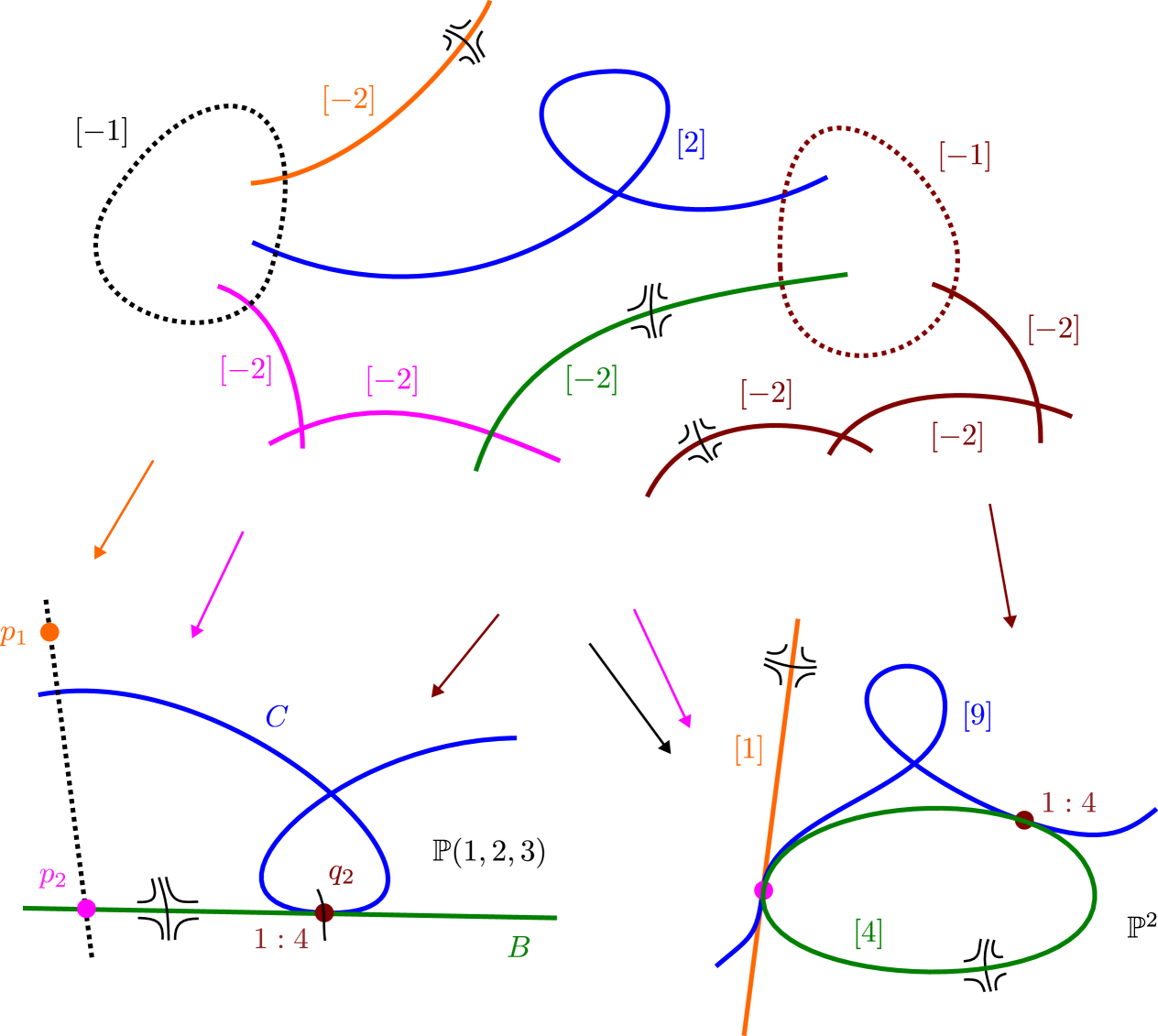
Figure 6. To the left, schematic resolution of singularities of $\mathcal{G}_{\mathrm{V}}$. To the right, a morphism to $\mathbb{P}^{2}$.

The birational involution coming from (21) reads

(27) $$[x:y:z]\mapsto[x^{3}-3xy+z:-x^{4}y+6x^{2}y^{2}-4xyz-y^{3}+z^{2}:\\ -x^{6}z+8x^{5}y^{2}-x^{4}yz-32x^{3}y^{3}+29x^{2}y^{2}z+8xy^{4}-12xyz^{2}-3y^{3}z+2z^{3}].$$

It is associated to the birational involution of $\mathbb{C}^{3}$ behind Theorem 7, which can be established by a direct computation.

4.2.1. Birational equivalence with $\mathcal{F}_{4}$

Under the birational map (14), $\mathcal{G}_{\mathrm{V}}$ is mapped to the degree-two foliation $\mathcal{H}_{4}$ of $\mathbb{P}^{2}$ given by (2). This establishes Theorem 3. The fact that the foliation is the unique one of degree two on $\mathbb{P}^{2}$ tangent to the cubic, conic and line follows from the fact that the tangency divisor of a pair of degree-two foliations on $\mathbb{P}^{2}$ has degree five.

Let us now study the singularities of the foliation. The previously described singular points $q_{1}$, $q_{2}$ and $q_{3}$ are, respectively, $(1:0:0)$, $(1:1:2)$ and $(9:3:2)$. On the line $x=0$, we have two singular points: $(0:1:4)$, a saddle with eigenvalues $-1:2$, and $(0:0:1)$, a nilpotent singularity with multiplicity three. The desingularization of $\mathcal{H}_{4}$ is given by the composition of the resolution $\pi:S\to\mathbb{P}(1,2,3)$ with the map $j$ in (14). See the right-hand side of Figure 6.

By conjugating the birational involution (27) via the birational map (14), we obtain:

Proposition 15.

The birational involution of $\mathbb{P}^{2}$ coming from (21), preserving the model (2) for $\mathcal{F}_{4}$, is the quartic transformation

$$(x:y:z)\mapsto(x(x-3y+z)^{3}:(x-3y+z)(6xy^{2}-x^{2}y-4xyz-y^{3}+xz^{2}):\\ 8x^{2}y^{2}-x^{3}z-x^{2}yz-32xy^{3}+29xy^{2}z+8y^{4}-12xyz^{2}-3y^{3}z+2xz^{3}).$$

The Jacobian of the latter is

$$4(x-y)^{4}(-3y+z+x)^{3}(x^{2}-4yx+2zx-y^{2}),$$

with the line $x-3y+z=0$ being tangent to the conic at $(1:1:2)$; the lines $y-x=0$ and $x-3y+z=0$ intersecting at $(1:1:2)$; and the line $y-x=0$ intersecting the conic at $(0:0:1)$ and $(1:1:2)$. Its homaloidal system is formed by plane quartics having ordinary triple points at $(1:1:2)$, and being smooth at $(0:0:1)$. One of the local branches at $(1:1:2)$ defines a contact direction of the elements of the system: four blow-ups are need to separate these elements, one at $(1:1:2)$ and three along the directions given by the contact branch. At $(0:0:1)$, three blow ups are need to separate the smooth curves. In the sense of [NTN20], it is a de Jonquières map of type $(4;3,1^{3};1^{3})$, i.e., of type 32.1 in Table 5.1, p. 96.

4.3. Chazy VI and $\mathcal{G}_{\mathrm{VI}}$

The associated vector field $W$ has the first integral

$$B=x^{6}-6x^{4}y+6zx^{3}-15x^{2}y^{2}+6xyz+8y^{3}-3z^{2},$$

of degree six, and the invariant hypersurface given by the quasihomogeneous polynomial of degree six

$$C=y^{2}x^{2}-xyz+z^{2}-3y^{3}.$$

These induce invariant curves for $\mathcal{G}_{\mathrm{VI}}$, the foliation induced by $W$ on $\mathbb{P}(1,2,3)$. The foliation $\mathcal{G}_{\mathrm{VI}}$ is regular at both $p_{1}$ and $p_{2}$; away from these, its singularities are

• $q_{1}=[1:0:0]$, with eigenvalues $\omega:1$;

• $q_{2}=[1:1:2]$, a linearizable node with eigenvalues $1:5$;

• $q_{3}=[6:6:12]$, a saddle with eigenvalues $-5:6$.

At $q_{2}$, $B$ has a node, and $C$ has a smooth branch tangent to the branch of $B$ in the direction of the eigenvalue $1$; the curves $B$ and $C$ have a contact of order $6$ at $q_{2}$. The curve $C$ has a node at $q_{1}$, and $B$ passes also through $q_{3}$.

Upon resolving the foliation at $q_{2}$, we find a chain of five invariant rational curves of self-intersection $-2$, given by the four invariant components in the desingularization of $q_{2}$ plus the strict transform of $B$; see the left-hand side of Figure 7. Its contraction gives a singularity of type $A_{5}$ which, together with $p_{1}$ and $p_{2}$, gives the three singularities in the quotient model of $\mathcal{F}_{6}$.

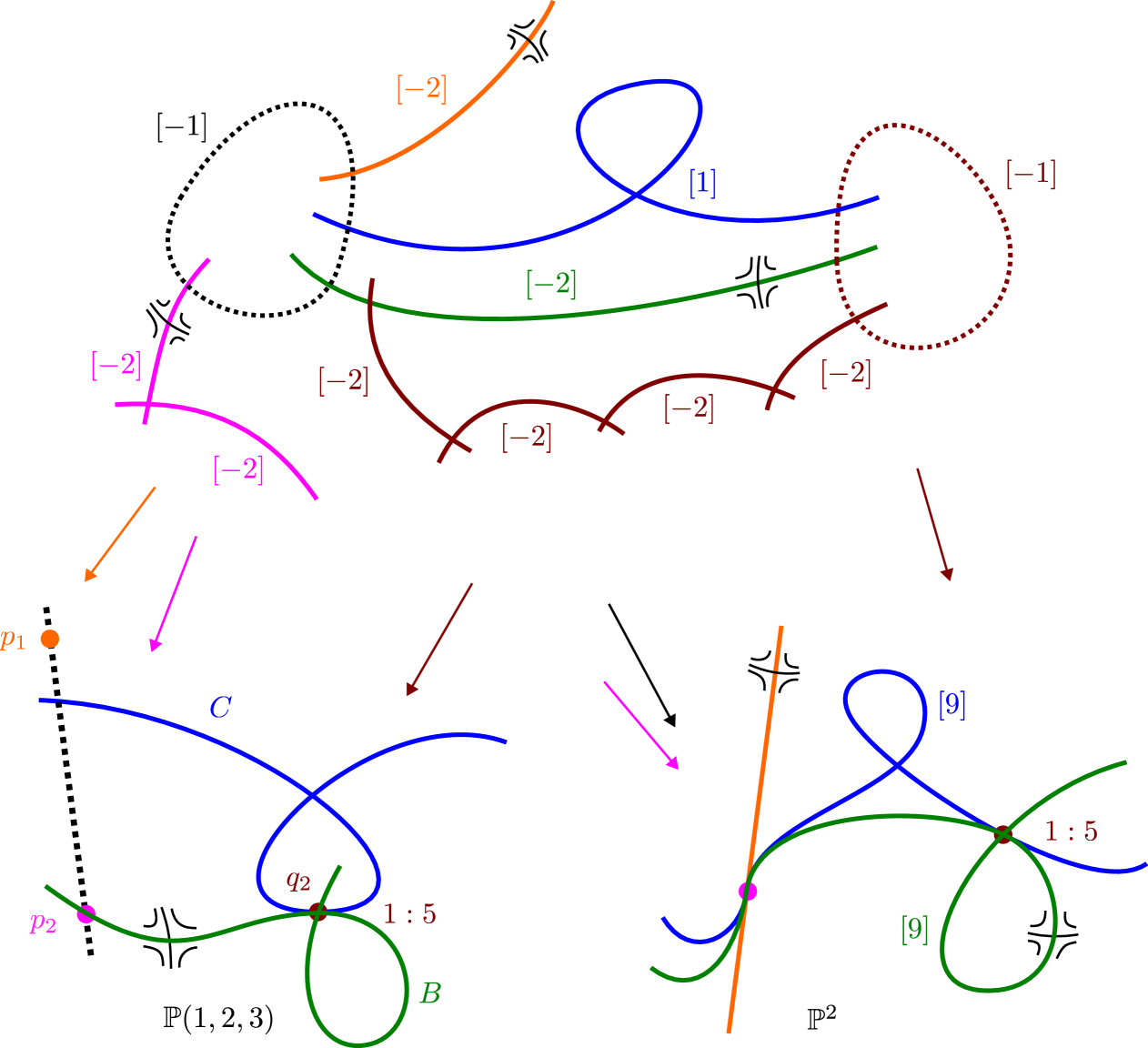
Figure 7. To the left, schematic resolution $\pi$ of singularities $\mathcal{G}_{\mathrm{VI}}$. To the right, a morphism to $\mathbb{P}^{2}$.

For $\Sigma=B^{-1}(1)$, we have a map $\Phi_{6}:\mathrm{Bl}_{3}(\mathbb{P}^{2})\to\Sigma$ [Gui12, p. 73], equivariant with respect to the actions of $\mathbb{Z}_{6}$ given the action of sixth roots of unity on $\Sigma$ via (7), and the action of $T_{6}$ on $\mathrm{Bl}_{3}(\mathbb{P}^{2})$ described in Section 3.3. It maps $\mathcal{E}_{6}$ to the foliation induced by $W$, and induces an identification of $\mathcal{G}_{\mathrm{VI}}$ with $\mathcal{F}_{6}$. From the explicit expressions for $\Phi_{6}$ and the inverse of $\Phi_{3}$ in [Gui12, p. 71], we may realize an explicit two-to-one map from $\mathbb{P}(1,2,3)$ to itself, mapping $\mathcal{G}_{\mathrm{IV}}$ to $\mathcal{G}_{\mathrm{VI}}$:

$$[x:y:z]\mapsto[xz-2y^{2}:3x^{4}y^{2}-3x^{3}yz-9x^{2}y^{3}+x^{2}z^{2}+8xy^{2}z+4y^{4}-3yz^{2}:\\ 9x^{6}y^{3}-12x^{5}y^{2}z-45x^{4}y^{4}+6x^{4}yz^{2}+63x^{3}y^{3}z-x^{3}z^{3}+\\ +54x^{2}y^{5}-42x^{2}y^{2}z^{2}-48xy^{4}z+15xyz^{3}-16y^{6}+18y^{3}z^{2}-3z^{4}].$$

It can be promoted to a rational map of $\mathbb{C}^{3}$ onto itself mapping the vector field corresponding to the Chazy IV equation to that of the Chazy VI one. This is the content of Theorem 8.

4.3.1. Birational equivalence with $\mathcal{F}_{6}$

Under the birational map (14), $\mathcal{G}_{\mathrm{VI}}$ is mapped to the degree two foliation of $\mathbb{P}^{2}$ given by (3). This establishes Theorem 3. That the foliation is the unique one of degree two on $\mathbb{P}^{2}$ tangent to both cubics follows, as before, from the fact that the tangency divisor of a pair of degree-two foliations on $\mathbb{P}^{2}$ has degree five.

The singularities in the complement of $x=0$ are those coming from $q_{1}$, $q_{2}$ and $q_{3}$, placed respectively at $(1:0:0)$, $(1:1:2)$ and $(18:3:1)$, with the same local descriptions as before. On the invariant line $x=0$, we have the singular point $(0:1:5)$, a saddle with eigenvalues $-1:2$, and $(0:0:1)$, a nilpotent singularity with multiplicity three. Its resolution is the composition of the resolution $\pi:S\to\mathbb{P}(1,2,3)$ with the map $j$ in (14). See the bottom-right of Figure 7.

5. Another plane model for Brunella’s foliation and its flop

In this section we will prove Theorem 9, that the degree two foliation $\mathcal{J}$ on $\mathbb{P}^{2}$ given by the form $\Omega$ in Eq. (10) is a planar model for Brunella’s very special foliation $\mathcal{F}_{3}$. In Section 5.2, we shall give another proof of the fact that the involutive Cremona map (11) represents the foliated flop.

The foliation $\mathcal{J}$ is tangent to the nodal cubic $C_{3}:xy^{2}-yz^{2}+zx^{2}-3xyz=0$, as well as to the lines of the coordinate triangle $\Delta_{3}:xyz=0$, each one of which is tangent to the cubic. Since a pair of degree-two foliations are either tangent along a curve of degree five or coincide, this is the only degree-two foliation tangent to this configuration. The singularities of $\mathcal{J}$ are:

• $(0:0:1)$ , $(0:1:0)$ and $(1:0:0)$, non-degenerate, with eigenvalues $1:2$, and which are linearizable, for they have two tangent invariant curves through them: $C_{3}$ and one of the coordinate lines;

• $(1:1:1)$, a reduced non-degenerate singularity with eigenvalues $-\omega:1$;

• $(0:2:1)$, $(2:1:0)$ and $(1:0:2)$, which are reduced and non-degenerate, have eigenvalues $-3:2$, and are not on $C_{3}$.

A (minimal) reduction of singularities of $\mathcal{J}$ is given by six blow ups: at each of the vertices $(0:0:1)$, $(0:1:0)$, $(1:0:0)$, and along the infinitely near points along the directions of the local branches of the cubic $C_{3}$. This is schematically presented in Figure 8.

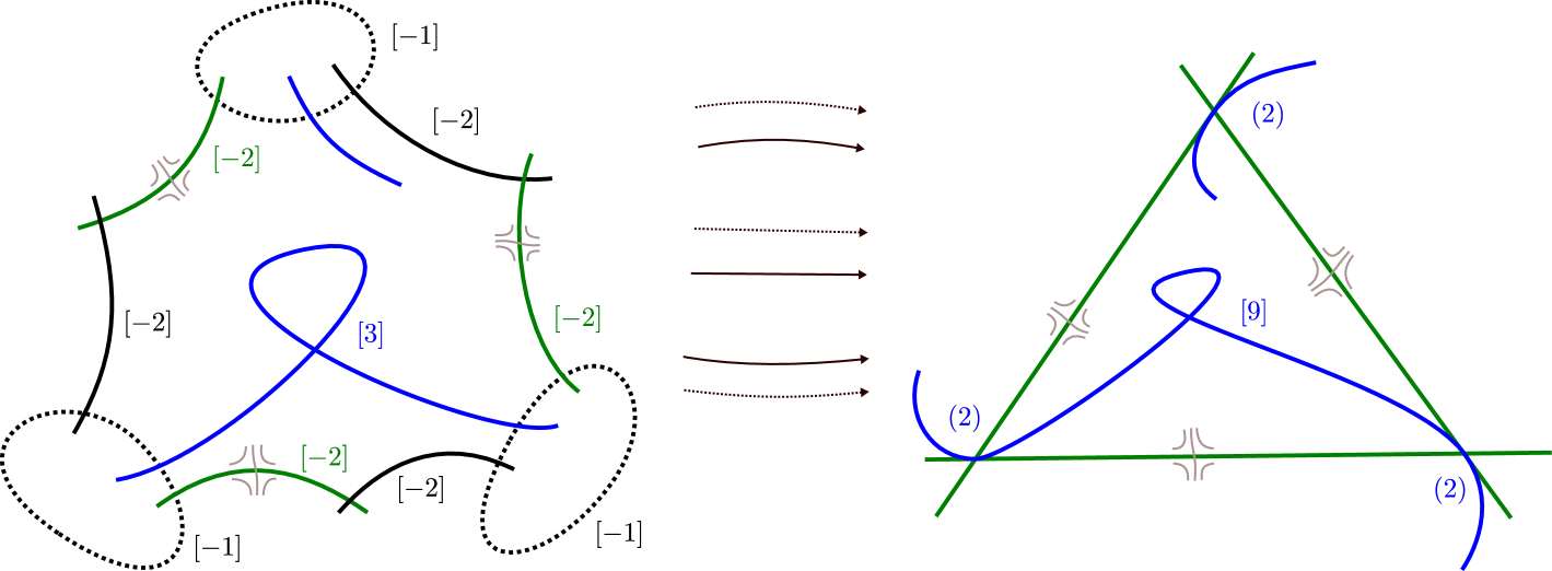
Figure 8. Reduction of singularities of $J$. Small gray curves are local separatrices.

In the blown-up projective plane in six points, the nodal curve has self-intersection $C_{3}^{2}=9-2-2-2=3$. The strict transforms of the lines of the triangle $\Delta_{3}$ and of the firstly introduced exceptional lines form three chains of two $(-2)$-curves in the blown-up plane (three $\mathcal{J}$-chains in the sense of [Bru15, Def. 8.1]), matching the combinatorics of the desingularization of a singularity of type $A_{2}$ each, as discussed in Section 2.2.

First proof of Theorem 9.

After blowing up, along $C_{3}$, there is just one reduced singularity, with eigenvalues $-\omega^{2}:1$. According to [Bru15] (Proposition 4.3), this characterizes the foliation $\mathcal{F}_{3}$ (up to birational equivalence). ∎

Second proof of Theorem 9.

For the form $\Xi$ of Eq. (26) defining Pereira’s model for $\mathcal{F}_{3}$, the quadratic Cremona map $Q_{2}(x:y:z)=(x^{2}:xy:zy)$, and the form $\Omega$ in Eq. (10), we have that $Q_{2}^{*}(\Xi)=x^{3}y\cdot\Omega$. This quadratic Cremona map establishes an explicit birational equivalence between Pereira’s model for $\mathcal{F}_{3}$ and the one presented in Theorem 9. ∎

The birational equivalence of this proof is schematically described in Figure 9.

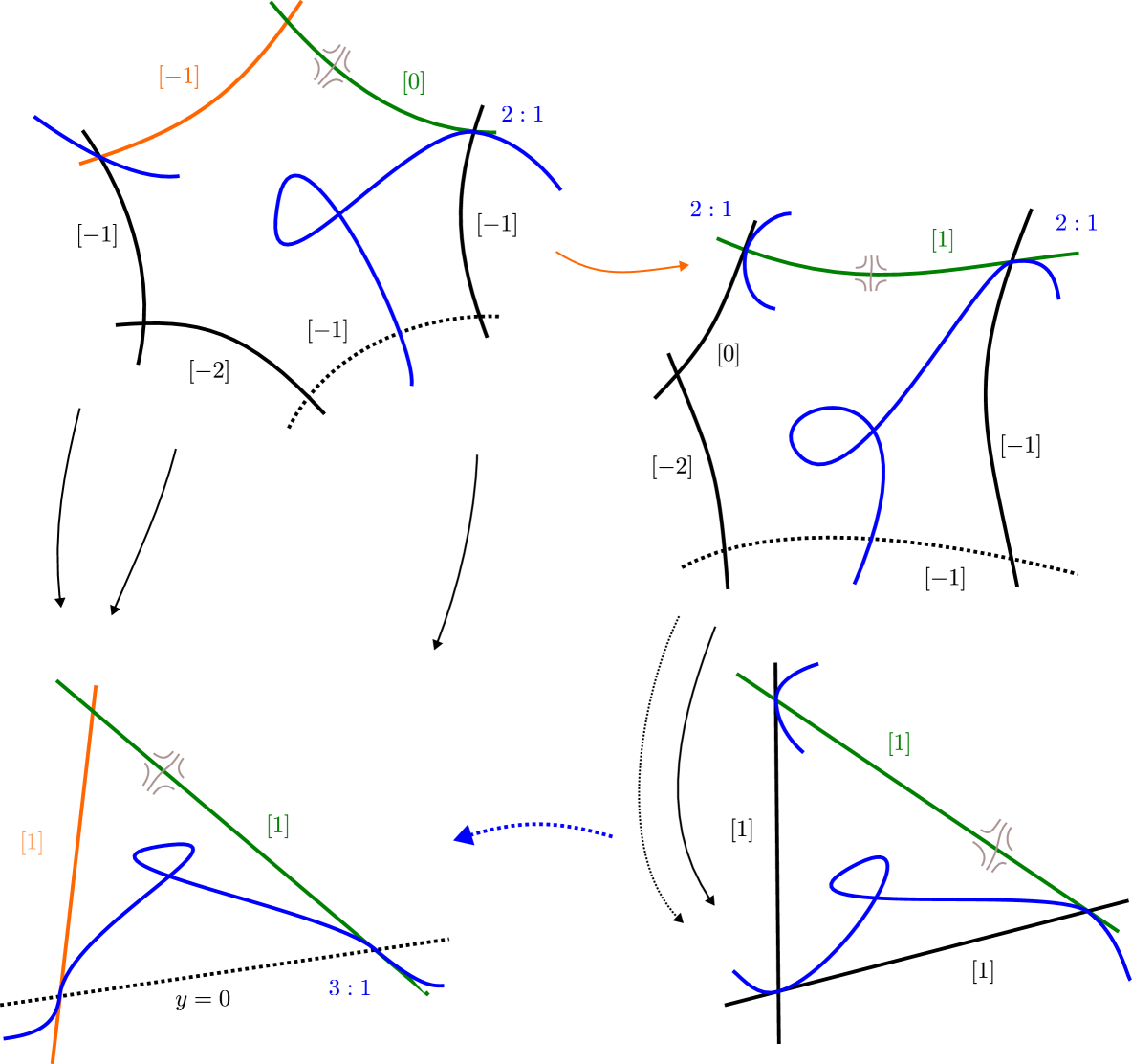
Figure 9. Birational equivalence between the two models for $\mathcal{F}_{3}$.

Third proof of Theorem 9.

Let us give a proof in the spirit of the study on the Chazy equations carried out in [Gui12]. Consider the quadratic homogeneous vector field on $\mathbb{C}^{3}$

(28) $$W=x(x-y)\frac{\partial}{\partial x}+y(y-z)\frac{\partial}{\partial y}+z(z-x)\frac{\partial}{\partial z},$$

which belongs to the kernel of (9) and projects to the foliation of $\mathbb{P}^{2}$ induced by it. It has the first integral $B=xyz$. Let $\Sigma=B^{-1}(1)$, parametrized by $(x,y)\mapsto(x,y,x^{-1}y^{-1})$. It has the order-three symmetry $\sigma:\Sigma\to\Sigma$ given by $\sigma(x,y)=(\omega x,\omega y)$, which preserves the foliation induced by $W$. The quotient of $\Sigma$, together with the induced foliation, identifies, via the projection $\pi:\mathbb{C}^{3}\setminus\{0\}\to\mathbb{P}^{2}$, to the foliation induced by $W$ in the complement of $B=0$ on $\mathbb{P}^{2}$. The map $j:\Sigma\to\mathbb{P}^{2}$,

$$j(x,y)=(xy+x+1:xy+\omega^{2}x+\omega:xy+\omega x+\omega^{2}),$$

maps $W|_{\Sigma}$ to the linear vector field $D_{3}$ on $\mathbb{P}^{2}$ given, in the affine chart $(X:Y:1)$, by (23). It has an inverse, given by

$$(X:Y:1)\mapsto\left(\frac{X+\omega Y+\omega^{2}}{X+\omega^{2}Y+\omega},\frac{X+Y+1}{X+\omega Y+\omega^{2}}\right),$$

and is thus a birational isomorphism. For the cyclic permutation of variables $T_{3}$ in (16), we have that $j\circ\sigma=T_{3}^{2}\circ j(x,y)$. This establishes a birational identification between the foliation on $\mathbb{P}^{2}$ induced by $W$ and the one on $\mathbb{P}^{2}/T_{3}$ induced by $\mathcal{E}_{3}$, Brunella’s very special foliation $\mathcal{F}_{3}$, as described in Section 3.1. ∎

The vector field (28) appearing in this proof is one of the scarce quadratic homogeneous ones having single-valued solutions (see [Gui06] for a general discussion of such vector fields).

Fourth proof of Theorem 9.

The map $\Phi:\mathbb{P}^{2}\dashrightarrow\mathbb{P}^{2}$ given by

$$(X:Y:Z)\mapsto((X+\omega Y+\omega^{2})^{2}(X+Y+1):\\ :(X+Y+1)^{2}(X+\omega^{2}Y+\omega):(X+\omega^{2}Y+\omega)^{2}(X+\omega\zeta Y+\omega^{2}))$$

realizes the quotient by the cyclic permutation of the coordinates. The pull-back of the form (15) by it is the form (10). (The map $\Phi$ is the composition $\pi\circ j^{-1}$ in the previous proof.) ∎

5.1. The de Jonquières symmetry

The Jacobian determinant of (11) is

$$4(x-y)^{2}(y-z)^{2}(x-z)^{2}(xy^{2}+yz^{2}+x^{2}z-3xyz);$$

its fixed curve is the quartic

$$x^{2}y^{2}+y^{2}z^{2}+x^{2}z^{2}-xy^{3}-yz^{3}-zx^{3}=0,$$

of geometrical genus two, having a node at $(1:1:1)$. The involution $J_{4}$ preserves the lines through $(1:1:1)$, and is thus of de Jonquières type. The homaloidal system of $J_{4}$ is formed by the quartic plane curves with an ordinary triple point in $(1:1:1)$, and tangencies at $(0:0:1)$, $(0:1:0)$, and $(0:0:1)$. In the sense of [NTN20], this de Jonquières map is of type $(4;3;1^{2};1^{2};1^{2})$, of type 78.1 in Table 5.1, p. 102.

For the effect of $J_{4}$ on $\Omega$,

$$J_{4}^{*}(\Omega)=(x-y)^{3}(y-z)^{3}(x-z)^{3}(xy^{2}+yz^{2}+x^{2}z-3xyz)\cdot\Omega;$$

it follows that $J_{4}$ is indeed a birational automorphism of the foliation $\Omega=0$.

Figure 10 shows the elimination of indeterminations of the de Jonquières map: on top, the projective plane blown-up seven times is portrayed, and the two $(-1)$-curves which are interchanged under the flop are singled out (compare with Figure 4).

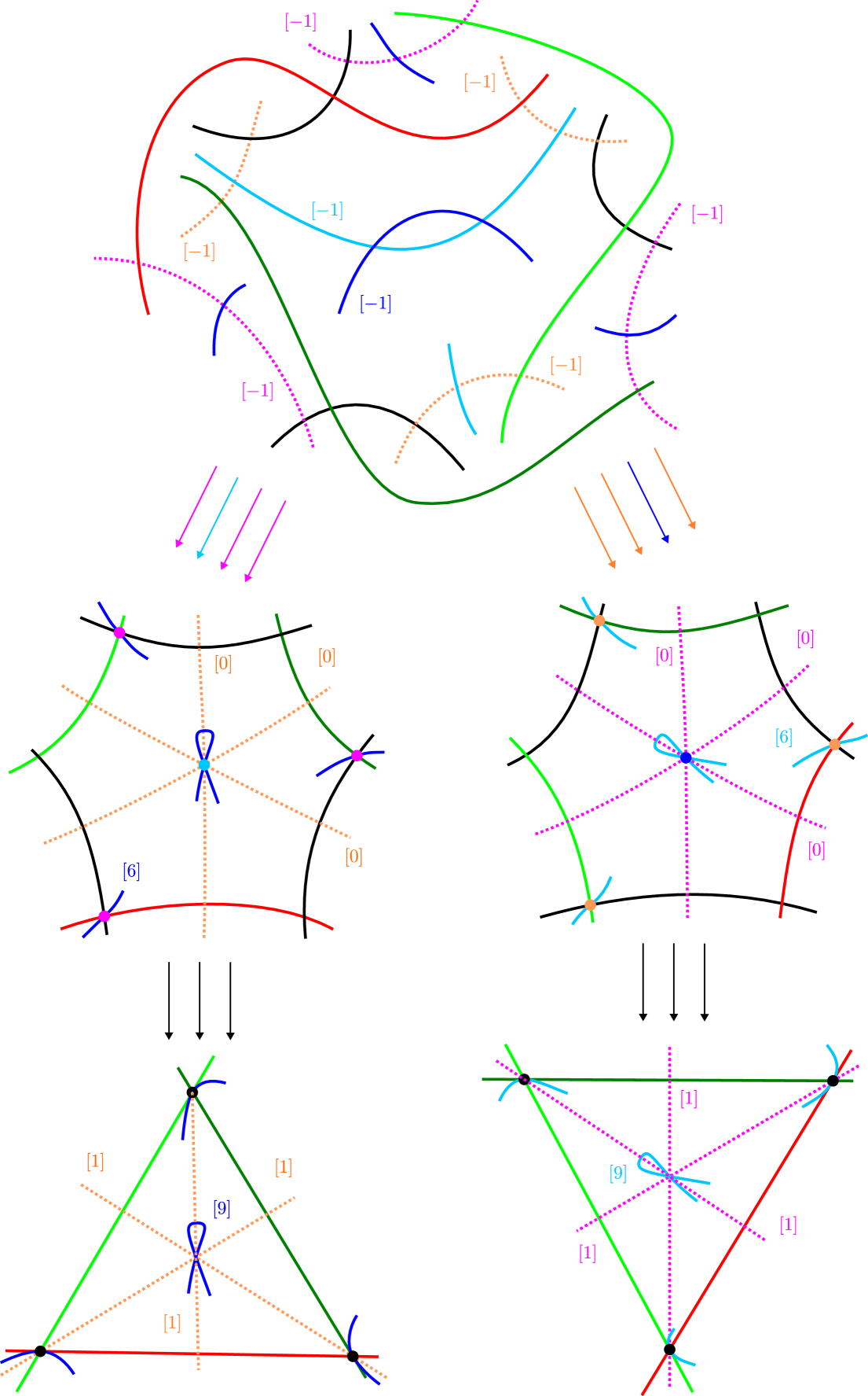
Figure 10. Diagram of elimination of indeterminations of $J_{4}$. The color of the arrow is the color of the exceptional line introduced by the blow-up.

In what follows, we will show that $J_{4}$ is the composition of three standard quadratic maps. This, and the proximity graph of Type 78.1, will show that its ordinary quadratic length (in the sense of [NTN20]) is three.

5.2. Factorization of the quartic de Jonquières involution

M. Noether established that every birational transformation of the complex projective plane may be factored as a composition of standard quadratic Cremona involutions and linear automorphisms. The varied and peculiar ways in which Cremona involutions may be composed to produce birational maps of small degrees bears witness to the complexity of this factorization; we refer the reader to recent works on the classification and factorization Cremona maps of degree three and four ([CD13], [CNTN22], [NTN20]) for a direct exposure to these.

We think that it is of interest to explicitly show that the quartic de Jonquières symmetry $J_{4}$ of $\mathcal{J}$ of Eq. (11) may be obtained as a composition of three standard quadratic Cremona maps; en passant, we shall give two models of $\mathcal{F}_{3}$ which are degree three foliations. In our planar model $\mathcal{J}$ for $\mathcal{F}_{3}$, a nodal plane cubic represents the link. So, in order to represent the foliated flop as a Cremona transformation of the plane, it is reasonable to try to obtain it as a composition of three quadratic Cremona maps which:

• gradually lower the degree of the cubic, from 3 to 2, from 2 to 1, and finally contract the line to a point and, at the same time,

• introduce a straight line, then increase its degree from 1 to 2, and finally from 2 to 3, producing a nodal cubic.

This plan is carried out in what follows. Through it, we shall prove once again that the involutive Cremona map (11) represents the foliated flop. The choices in the changes of coordinates that follow were guided by Proposition 12.

5.2.1. The first quadratic map and its effect on the foliation

We start with the foliation $\mathcal{J}$ on $\mathbb{P}^{2}$ given by the form $\Omega$ in Eq. (10), with its invariant nodal cubic $C_{3}:y^{2}x+z^{2}y+zx^{2}-3xyz=0$ and shall apply to it a quadratic Cremona map.

Consider the linear automorphism $L_{1}(x:y:z):=(x:x+y:x+z),$ which fixes $(0:0:1)$ and $(0:1:0)$, and maps $(1:0:0)$ to $(1:1:1)$, and the standard quadratic Cremona map $Q$ of Eq. (17). The strict transform of the foliation $\mathcal{J}$ by the quadratic Cremona map $Q\circ L_{1}^{-1}$ is the degree three foliation $\mathcal{J}^{\prime}$ given by the vanishing of

$$\Omega^{\prime}=yz(2xy-yz+z^{2}+y^{2}-xz)\,\mathrm{d}x-xz(z+y)(x+z)\,\mathrm{d}y-xy(y-2z)(x+y)\,\mathrm{d}z.$$

The invariant conic $C_{2}:y^{2}-yz+xy+z^{2}=0$ is the strict transform of $C_{3}$. The birational image of the nodal point $(1:1:1)$ of $C_{3}$ is the $\mathcal{J}^{\prime}$-invariant line $D_{1}:x=0$. Besides $C_{2}$ and $D_{1}$, $\mathcal{J}^{\prime}$ leaves invariant four straight lines. The foliations $\mathcal{J}$ and $\mathcal{J}^{\prime}$ are depicted in Figure 11.

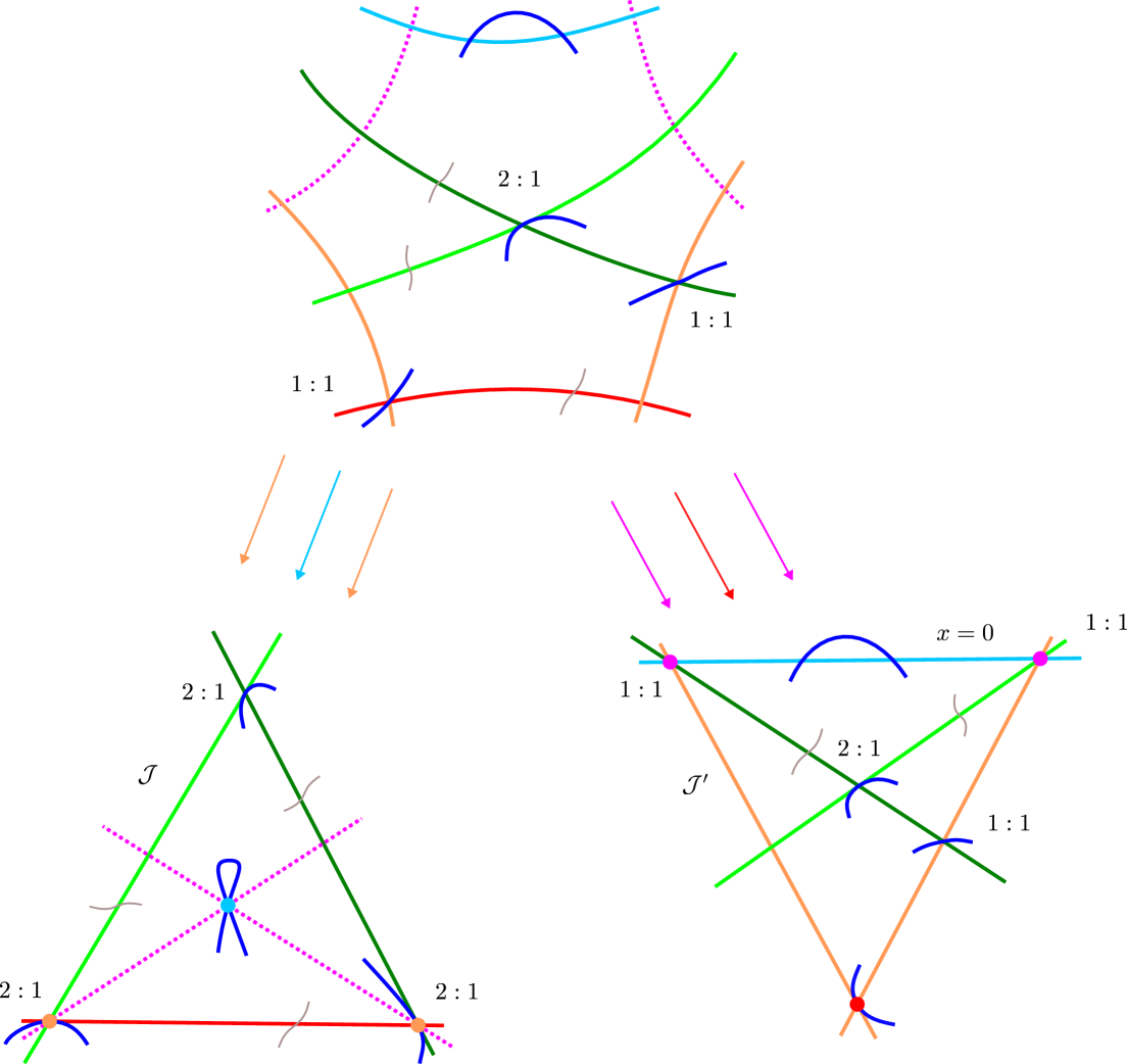
Figure 11. Effect of the first quadratic Cremona map on the foliation; the indetermination points are in red and blue. The representation of the node is schematic; it is an acnode in the real plane.

The singularities of $\mathcal{J}^{\prime}$ are:

• at $(0:0:1)$, $(0:1:0)$, $(-1:1:0)$: radial points (indicated by $1:1$ in Figure 11);

• at $(0:1:-\omega)$, $(0:1:-\omega^{2})$, $(-1:0:1)$, $(1:-1:1)$, and $(-1:2:1)$: five non-degenerate singularities (the first two are the intersection $C_{2}\cap D_{1}$);

• at $(-1:1:1)$: with eigenvalues $1:2$, linearizable;

• at $q=(1:0:0)$ (in red in the bottom-right of Figure 11): a quadratic non-dicritical singularity ($\nu(p)=l(p,\mathcal{J}^{\prime})=2$). Its Milnor number $\mu(q,\mathcal{J}^{\prime})=4$ can be computed directly through formula (13), observing that there are three points with $\mu=1$ along the line blown down to it (in red in the top of Figure 11), or using Darboux’s formula (Proposition 11), and taking into account that the other nine listed singularities have Milnor number $\mu=1$.

5.2.2. The second quadratic map and its effect on the foliation

Consider now the linear map $L_{2}(x:y:z):=(x-y+z:y-z:-z),$ which fixes $(1:0:0)$, and maps $(0:0:1)$ and $(0:1:0)$ to $(-1:1:1)$ and $(-1:1:0)$, respectively. The strict transform of $\mathcal{J}^{\prime}$ by the quadratic map $Q\circ L_{2}^{-1}$ is the degree three foliation $\mathcal{J}^{\prime\prime}$ given by the vanishing of

$$\Omega^{\prime\prime}=z(z-y)(2yz-y^{2}-xz+2xy)\,\mathrm{d}x+xz(2yz-z^{2}-2xz+xy)\,\mathrm{d}y+\\ +x(y^{2}-yz+z^{2})(x-y)\,\mathrm{d}z.$$

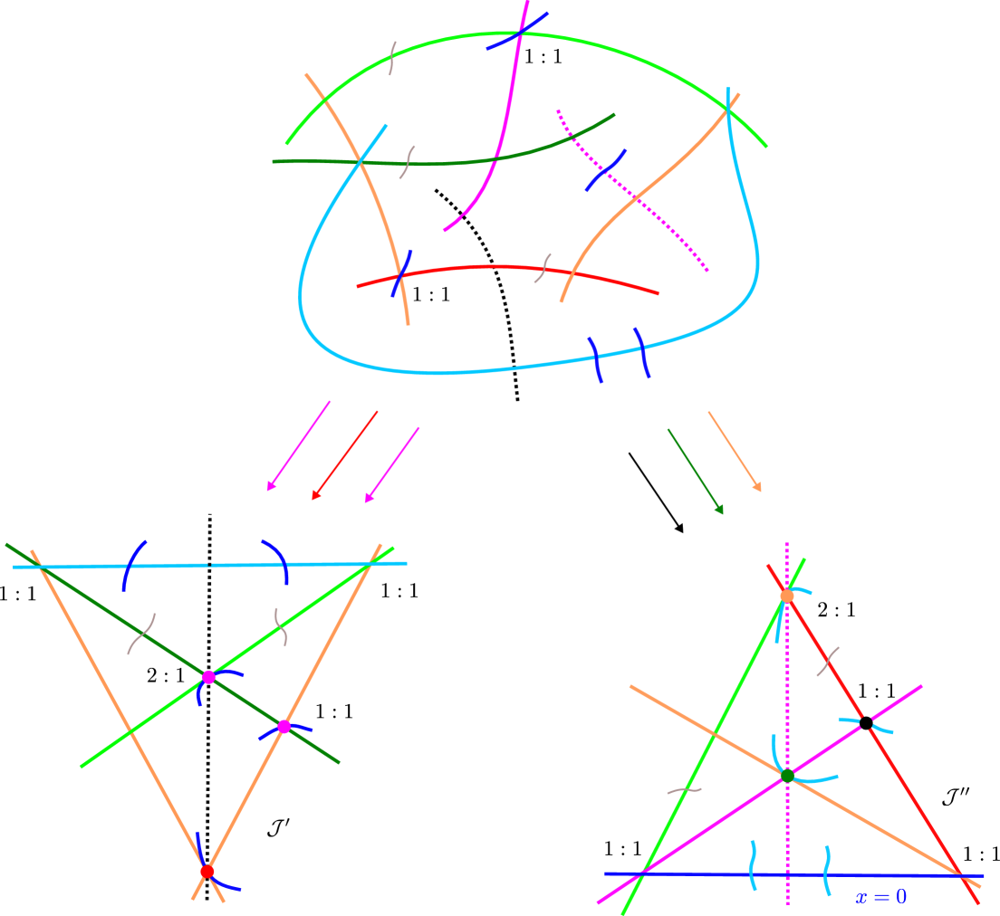
Figure 12. Effect of the second quadratic Cremona map on the foliation; the indetermination points are in red and magenta.

This is portrayed in Figure 12. The singular set of $\mathcal{J}^{\prime\prime}$ is of exactly the same type as the one of $\mathcal{J}^{\prime}$, but the singularities appear in different positions (for instance, the quadratic non-dicritical singularity is the green point in the bottom-right of Figure 12, blow-down of the green line on top). The strict transform of the conic $C_{2}:y^{2}-yz+xy+z^{2}=0$ is the line $C_{1}:x-y+z=0$, and the strict transform of the line $D_{1}:x=0$ is the conic $D_{2}=yz-xz+xy=0$.

5.2.3. The third quadratic map and its effect on the foliation

Consider now the linear map $L_{3}(x:y:z):=(x+z:z+y:y),$ which fixes $(1:0:0)$, and maps $(0:0:1)$ and $(0:1:0)$, to $(1:1:0)$ and $(0:1:1)$, respectively. The strict transform of $\mathcal{J}^{\prime\prime}$ by the quadratic map $Q\circ L_{3}^{-1}$ is the degree-two foliation $\mathcal{J}^{\prime\prime\prime}$ given by the vanishing of

$$\Omega^{\prime\prime\prime}=z(xy+xz+y^{2}x+zy+2y^{2})\,\mathrm{d}x-x(2z+y)(x+z)\,\mathrm{d}y+x(y-z)(x-y)\,\mathrm{d}z.$$

The line $C_{1}:x-y+z=0$ is contracted to the point $(1:0:0)$ by this third quadratic Cremona map and the strict transform of the conic $D_{2}:yz-xz+xy=0$ is the nodal cubic $D_{3}:xyz+xz^{2}+y^{2}z+y^{2}x=0$, having a node at $(1:0:0)$. See Figure 13.

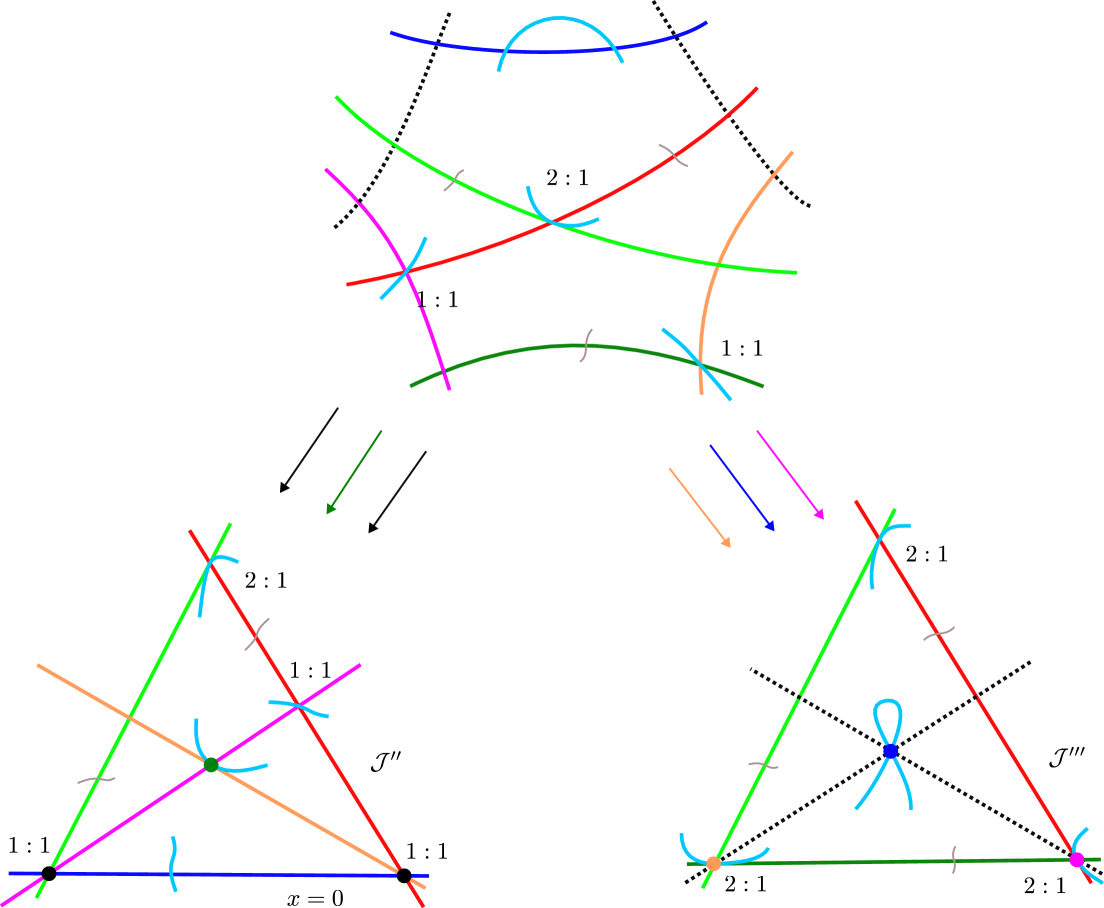
Figure 13. Effect of the third Cremona map on the foliation. The indetermination points are in black and green.

We assert that this last foliation $\mathcal{J}^{\prime\prime\prime}$ is isomorphic to the original foliation $\Omega=0$ of Eq. (10). In fact, for the linear isomorphism $L_{4}(x,y,z):=(ax,\,a(x-z),\,a(y-x))$, for $a=\frac{\sqrt{2}}{2}(1+\mathrm{i})$, we have $L_{4}^{*}(\Omega^{\prime\prime\prime})=\Omega$.

Finally, composing the three quadratic transformations $Q\circ L_{j}^{-1}$, $j=1,2,3$, and $L_{4}^{-1}$, we obtain (after extracting common factors) the map $J_{4}$ of Eq. (11), $J_{4}=L_{4}^{-1}\circ Q\circ L_{3}^{-1}\circ Q\circ L_{2}^{-1}\circ Q\circ L_{1}^{-1}$.

6. Quotients of linear foliations by standard quadratic Cremona involutions

The exceptionality of the automorphisms of linear foliations leading to the foliations of Brunella and Santos may be also brought to light through the study of the birational symmetries of linear foliations; we will study this in Section 7. There, we will also see that most linear foliations of the plane have only one non-linear birational automorphism (up to linear conjugation), the standard quadratic Cremona involution. The question of understanding the associated quotient foliations follows naturally. In this section, we will prove Theorem 12, giving explicit plane models for these foliations.

6.1. Cayley’s nodal cubic as the quotient under the standard quadratic involution

Recall that Cayley’s nodal cubic surface is the surface $M_{3}$ in $\mathbb{P}^{3}$ given in homogeneous coordinates $(\xi:\eta:\zeta:\theta)$ by

(29) $$\xi\eta\zeta+\xi\eta\theta+\xi\zeta\theta+\eta\zeta\theta=0.$$

It has four singularities, which are nodal points (this is, they are of type $A_{1}$), at $(1:0:0:0)$, $(0:1:0:0)$, $(0:0:1:0)$ and $(0:0:0:1)$. It is the only cubic surface having four nodal points. It contains nine lines: six connecting a pair of nodes each, forming a tetrahedron; and three, coplanar, connecting pairs of points within the triple $(1:1:-1:-1)$, $(1:-1:1:-1)$, $(1:-1:-1:1)$, the lines $\xi+\eta=\zeta+\theta=0$, $\xi+\zeta=\eta+\theta=0$, and $\xi+\theta=\eta+\zeta=0$. The surface has no other lines. The group $S_{4}$ acts on $M_{3}$ by permuting the homogeneous coordinates, and naturally permutes all the above objects. See Figure 14.

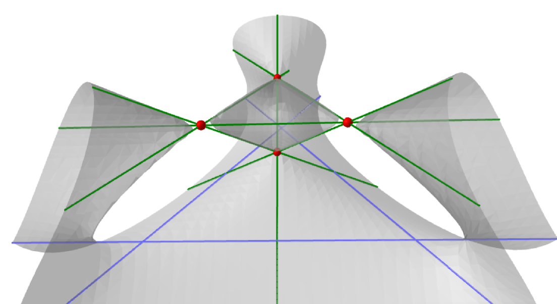
Figure 14. Cayley’s nodal cubic surface.

We will begin by showing that the quotient of $\mathbb{P}^{2}$ under the action of the standard quadratic Cremona involution $Q(X:Y:Z)=(YZ:ZX:XY)$ is Cayley’s nodal cubic surface (see also [Emc26, Section II.A]). Consider the $Q$-invariant rational map $\pi:\mathbb{P}^{2}\dashrightarrow\mathbb{P}^{3}$,

$$(\xi:\eta:\zeta:\theta)=(X(Y^{2}+Z^{2}):Y(X^{2}+Z^{2}):Z(X^{2}+Y^{2}):2XYZ),$$

whose coordinates form a basis for the space of homogeneous cubic polynomials $P$ such that $P(YZ,ZX,XY)=XYZ\,P(X,Y,Z)$. It realizes the quotient of $\mathbb{P}^{2}$ by $Q$.

Let $\overline{\pi(\mathbb{P}^{2})}$ be the surface in $\mathbb{P}^{3}$ which is the rational image of $\mathbb{P}^{2}$ by $\pi$. It has the cubic equation

$$\overline{\pi(\mathbb{P}^{2})}:\,\theta(\xi^{2}+\eta^{2}+\zeta^{2})-2\xi\eta\zeta-\theta^{3}=0.$$

The four fixed points of $Q$ produce, via $\pi$, four singular points of type $A_{1}$ for $\overline{\pi(\mathbb{P}^{2})}$, placed at $(-1:-1:1:1)$, $(-1:1:-1:1)$, $(1:-1:-1:1)$ and $(1:1:1:1)$. The linear transformation

$$L(\xi:\eta:\zeta:\theta)=(\theta+\xi-\eta-\zeta:\theta-\xi+\eta-\zeta:\theta-\xi-\eta+\zeta:\theta+\xi+\eta+\zeta)$$

establishes a linear isomorphism between $\overline{\pi(\mathbb{P}^{2})}$ and Cayley’s nodal cubic (29), and maps the above singular points to the nodes on Cayley’s surface.

The map $L\circ\pi$ realizes the quotient of $\mathbb{P}^{2}$ under the action of the standard quadratic Cremona involution as Cayley’s nodal cubic surface.

6.2. A birational plane model

Let us take a step further, and pass from Cayley’s surface to a new copy of the projective plane. The strict transform of Cayley’s cubic surface $M_{3}$ by the cubic involutive Cremona map of $\mathbb{P}^{3}$

$$C(\xi:\eta:\zeta:\theta)=(\eta\zeta\theta:\xi\zeta\theta:\xi\eta\theta:\xi\eta\zeta),$$

is the plane $A\subset\mathbb{P}^{3}$ with equation $\xi+\eta+\zeta+\theta=0$. Consider the mapping $j:\mathbb{P}^{2}\to A$,

$$(X:Y:Z)\mapsto(X:Y:Z:-X-Y-Z).$$

Let $\Pi:\mathbb{P}^{2}\dashrightarrow\mathbb{P}^{2}$ be the composition $j^{-1}\circ C\circ L\circ\pi$, which reads:

(30) $$\Pi(X:Y:Z)=((Z+Y)(Z+X)(Y-X):(Z+Y)(X-Z)(X+Y):(Z-Y)(Z+X)(X+Y)),$$

and has Jacobian

(31) $$-12(Y-X)(Y+X)(Z-Y)(Z+Y)(Z+X)(Z-X).$$

The map $\Pi$ in (30) realizes $\mathbb{P}^{2}$ as a birational model for the quotient of $\mathbb{P}^{2}$ under the action of the standard quadratic Cremona involution.

6.3. The quotient foliations

Let $\lambda\in\mathbb{C}\setminus\{0,1\}$, and consider the degree-one foliation $\mathcal{F}_{\lambda}$ on $\mathbb{P}^{2}$ induced by

(32) $$w_{\lambda}=\lambda YZ\,\mathrm{d}X-XZ\,\mathrm{d}Y+(1-\lambda)XY\,\mathrm{d}Z.$$

It is preserved by the standard quadratic Cremona map $Q$. There is a remarkable configuration in $\mathbb{P}^{2}$ associated to the Cremona involution, the complete quadrangle associated to its four fixed points, presented in Figure 15. In it we have, in red, the four fixed points of $Q$, placed at $(1:1:1)$, $(-1:1:1)$, $(1:-1:1)$ and $(1:1:-1)$. The dashed green lines are those of the configuration $\mathcal{L}_{6}$, the six lines joining pairs of fixed points of $Q$, along which the Jacobian of $\Pi$ (31) vanishes. They are transverse to the foliation and preserved by $Q$, which restricts to each one of them as an involution. The pairs of lines of $\mathcal{L}_{6}$ that do not share a common fixed point of $Q$ intersect, by pairs, at the three indeterminacy points of $Q$, $(1:0:0)$, $(0:0:1)$ and $(0:0:1)$. The three lines through these points, in blue in Figure 15, are those of the coordinate triangle $\Delta_{3}:XYZ=0$, and are $\mathcal{F}_{\lambda}$-invariant. The Cremona involution $Q$ contracts these lines, while blowing up the vertices of the triangle; it exchanges a line of the triangle with its opposite vertex.

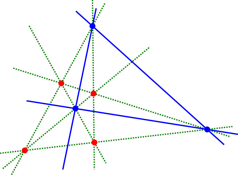
Figure 15. The complete quadrangle associated to the four fixed points of the standard quadratic Cremona involution.

Figure 16 focuses in the coordinate triangle $\Delta_{3}$ and the eigenvalues of the vector field at the singular points of $\mathcal{F}_{\lambda}$.

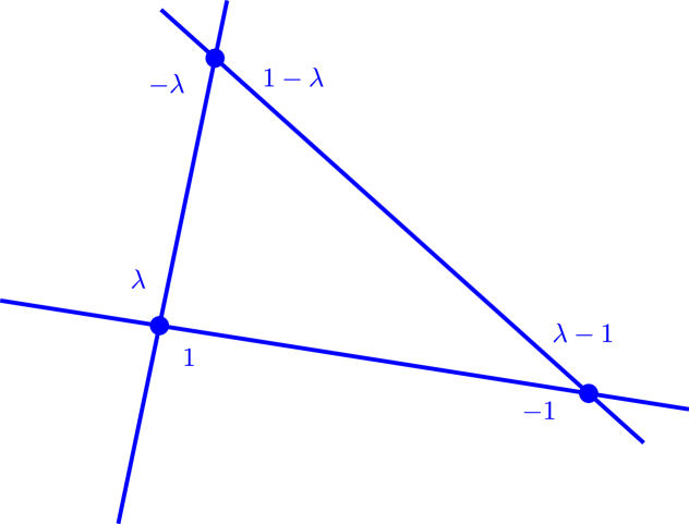
Figure 16. The coordinate triangle, invariant by $\mathcal{F}_{\lambda}$, and the corresponding eigenvalues.

The foliation $\mathcal{F}_{\lambda}$ induces a foliation on the quotient of $\mathbb{P}^{2}$ under the action of $Q$. In the birational plane model for this quotient given by $\Pi$, this foliation is the foliation $\mathcal{G}_{\lambda}$ given by the form (12), a fact that can be established trough a direct calculation, proving Theorem 10. Let us nevertheless explain how the form (12) was obtained, and describe the geometry of both $\Pi$ and the foliation $\mathcal{G}_{\lambda}$.

Consider the vector space $\Omega_{3}$ of one-forms on $\mathbb{C}^{3}$ of the form $A\,\mathrm{d}x+B\,\mathrm{d}y+C\,\mathrm{d}z$, with $A$, $B$ and $C$ homogeneous polynomials of degree four in $x,y,z$. Consider also the linear homogeneous vector fields $E=X\,\partial/\partial X+Y\,\partial/\partial Y+Z\,\partial/\partial Z$ and $V=X\,\partial/\partial X+\lambda^{2}Y\,\partial/\partial Y-\lambda Z\,\partial/\partial Z$, which are linearly independent on a Zariski-open subset, and which are in the kernel of the form (32) generating $\mathcal{F}_{\lambda}$. Within $\Omega_{3}$, the elements $w$ for which the conditions $(\Pi^{*}w)E\equiv 0$ and $(\Pi^{*}w)V\equiv 0$ hold is a linear subspace, that may be defined by explicit linear equations on the coefficients of the polynomials $A$, $B$ and $C$. By solving this system, this subspace is found to have dimension one, and to be generated by the form (12).

The foliation $\mathcal{G}_{\lambda}$ is tangent to a remarkable configuration, independent of $\lambda$, which we present in Figure 17. On the target plane of $\Pi$, with coordinates $(x:y,z)$, consider the quadrilateral formed by the lines

$$xyz(x+y+z)=0,$$

(in red in Figure 17), together with its six vertices, the points of intersection of each pair of lines of the quadrilateral: $(0:0:1)$, $(0:1:0)$, $(1:0:0)$, $(-1:0:1)$, $(0:-1:1)$ and $(-1:1:0)$, in green in Figure 17. These six points come in three pairs (pairs without a common line), and each pair determines a line; these are the diagonals

$$(x+y)(x+z)(y+z)=0,$$

in blue in Figure 17. The three points of intersection of the diagonals are the diagonal points, $(-1:1:1)$, $(1:-1:1)$ and $(1:1:-1)$. Each line of the quadrilateral is incident to three vertices. Each diagonal is incident to two vertices and two diagonal points. Each vertex lies on two sides of the quadrilateral and one diagonal. Each diagonal point lies on two diagonals.

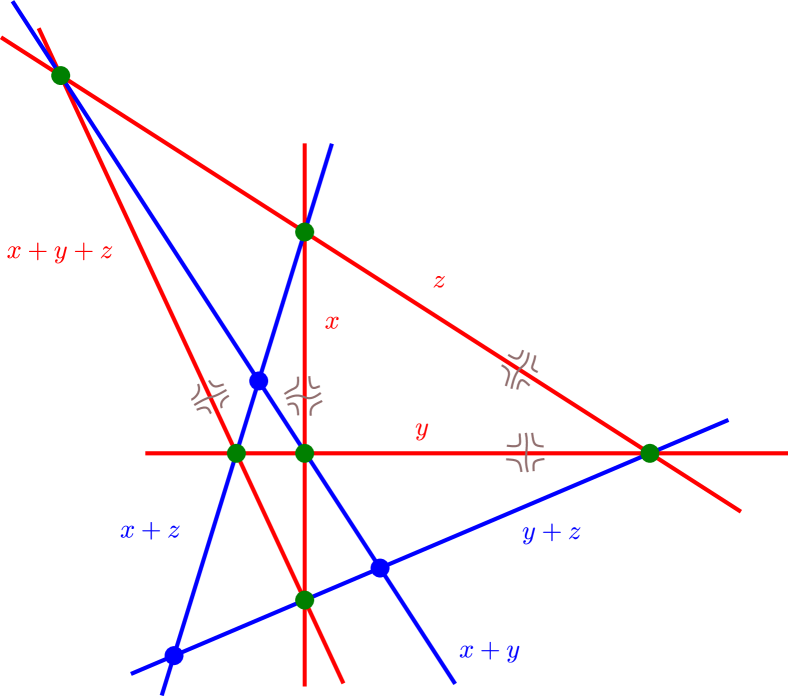
Figure 17. The complete quadrilateral and its diagonals, in the model after quotient by the involution. The lines appear in red, the vertices in green, the diagonals and the diagonal points in blue.

The seven lines of this configuration are tangent to the foliation $\mathcal{G}_{\lambda}$, and its nine points are singular points of the foliation, which has four further singular points, one on each line of the quadrilateral, with eigenvalues $-2:1$, and whose position depends upon $\lambda$. These account for all thirteen singular points of the degree three foliation $\mathcal{G}_{\lambda}$, the number of singularities of a degree three foliation in the plane (counted with multiplicity).

The four fixed points of $Q$ are mapped by $L\circ\pi$ to the nodes of $M_{3}$, which are in turn mapped by $j^{-1}\circ C$ to the four sides of the quadrilateral (here, and in what follows, when we refer to the image of a curve by a rational map we always mean its strict transform). The six lines in $\mathcal{L}_{6}$ joining these by pairs are mapped by $L\circ\pi$ to the six edges of the tetrahedron in $M_{3}$, and then by $j^{-1}\circ C$ to the six vertices of the quadrilateral, which are radial singularities for $\mathcal{G}_{\lambda}$, as expected from the fact that the lines of $\mathcal{L}_{6}$ are transverse to the foliation. The strict transform by $L\circ\pi$ of each of the lines of the coordinate triangle $\Delta_{3}$ is one of the three coplanar lines of $M_{3}$ that do not pass through its singular points (for $X=0$, the line $\xi+\eta=\zeta+\theta=0$; for $Y=0$, the line $\xi+\zeta=\eta+\theta=0$; and for $Z=0$, the line $\xi+\theta=\eta+\zeta=0$). These are then mapped by $j^{-1}\circ C$ to the three diagonals. Figure 18 focuses on the triangle formed by these diagonals, and presents the eigenvalues of the linear parts of the singularities at its vertices.

Figure 18. Ratios of eigenvalues at the singularities of $\mathcal{G}_{\lambda}$ on the blue lines.

Remark 16.

The classical del Pezzo surfaces of degree three are the images of the plane under a system of cubics passing by six points in general position. Although the six triple points of the previous arrangement (in green in Figure 17) are not in general position, they impose independent conditions on cubics, and define a rational map from the plane to a singular cubic surface of $\mathbb{P}^{3}$, linearly isomorphic to Cayley’s nodal cubic. Therefore, the foliations $\mathcal{G}_{\lambda}$ can be regarded as foliations of a singular del Pezzo surface.

By blowing up the six vertices of the quadrilateral (the triple points of the configuration) each one of its four lines becomes a curve of self-intersection $-2$, corresponding to the resolution of a singularity of type $A_{1}$. The triangle formed by the diagonals becomes a cycle of three curves of self-intersection $-1$.

7. The groups of birational automorphisms of the special quotient foliations

Theorem 5 will be proved in this section. To a holomorphic foliation by curves on an algebraic manifold, we can associate the space of its Zariski-dense leaves, a (not-necessarily-Hausdorff) complex manifold. This space is a birational invariant, and the group of birational transformations preserving the foliation acts holomorphically on it. In the cases we consider, these spaces are either elliptic curves or their quotients under the action of a finite group acting with fixed points (elliptic orbifolds), and, for all of these, the groups of biholomorphisms can be easily described. This will be the starting point for Theorem 5.

7.1. Birational symmetries of linear foliations

We begin by describing the groups of birational automorphisms of the hyperbolic linear foliations of the projective plane.

Let $\mathbb{H}=\{\tau\in\mathbb{C}\mid\Im(\tau)>0\}$. For $\tau\in\mathbb{H}$, let $\mathcal{L}_{\tau}$ be the linear foliation on $\mathbb{P}^{2}$ given in the chart $(x:y:1)$ by the vector field $X_{\tau}=\tau x\,\partial/\partial x+y\,\partial/\partial y$. Consider two actions of $\mathrm{SL}(2,\mathbb{Z})$: the first, by fractional linear transformations on $\mathbb{H}$,

(33) $$\left(\begin{array}[]{cc}a&b\\ c&d\end{array}\right)\cdot\tau=\frac{a\tau+b}{c\tau+d};$$

and, the second, by monomial birational transformations on $\mathbb{P}^{2}$,

(34) $$\left(\begin{array}[]{cc}a&b\\ c&d\end{array}\right)\cdot(x:y:1)=(x^{a}y^{b}:x^{c}y^{d}:1).$$

With respect to these, for $A\in\mathrm{SL}(2,\mathbb{Z})$,

$$A_{*}\mathcal{L}_{\tau}=\mathcal{L}_{A\cdot\tau}.$$

In particular, if $A\in\mathrm{SL}(2,\mathbb{Z})$ stabilizes $\tau\in\mathbb{H}$ via the action (33), its action on $\mathbb{P}^{2}$ via (34) is a birational automorphism of $\mathcal{L}_{\tau}$. For example, as we have seen in Section 6, the action of $\left(\begin{array}[]{rr}-1&0\\ 0&-1\end{array}\right)$ via (34), the standard quadratic Cremona transformation, is a birational automorphism of $\mathcal{L}_{\tau}$ for every $\tau\in\mathbb{H}$.

In this setting, we may describe the group of birational automorphisms of $\mathbb{P}^{2}$ that preserve $\mathcal{L}_{\tau}$:

Theorem 17.

Let $\tau\in\mathbb{H}$. Let $\mathrm{Bir}(\mathbb{P}^{2},\mathcal{L}_{\tau})$ be the group of birational transformations of $\mathbb{P}^{2}$ that preserve $\mathcal{L}_{\tau}$. Let $G_{\tau}^{0}\subset\mathrm{PGL}(3,\mathbb{C})\cap\mathrm{Bir}(\mathbb{P}^{2},\mathcal{L}_{\tau})$ be the subgroup generated by the flows of $X_{\tau}$ and $x\,\partial/\partial x$. Let $I_{\tau}\subset\mathrm{SL}(2,\mathbb{Z})$ be the stabilizer of $\tau$ under the action (33). The group $\mathrm{Bir}(\mathbb{P}^{2},\mathcal{L}_{\tau})$ is the semidirect product $I_{\tau}\ltimes G_{\tau}^{0}$, with $I_{\tau}$ acting birationally on $\mathbb{P}^{2}$ via the monomial action (34).

The result will be straightforward consequence of the upcoming Proposition 19 and its proof. The spaces of transcendental leaves will establish a link between the problem at hand and that of the classification of elliptic curves.

Let $\Lambda_{\tau}\subset\mathbb{C}$ the lattice generated by $1$ and $\tau$, and let $E_{\tau}$ be the elliptic curve $\mathbb{C}/\Lambda_{\tau}$. The group of deck transformations of the universal covering $\mathbb{C}\to E_{\tau}$ is isomorphic to $\mathbb{Z}^{2}$, and given by

(35) $$\gamma_{m,n}(z)=z+m+n\tau.$$

Let $U\subset\mathbb{P}^{2}$ be the complement of the three coordinate lines, with coordinates $(x:y:1)$. It is saturated by $\mathcal{L}_{\tau}$, and has Zariski-dense leaves exclusively. Consider the map $f_{\tau}:U\to E_{\tau}$,

$$f_{\tau}(x,y)=\frac{1}{2\mathrm{i}\pi}(\log(x)-\tau\log(y))\mod\Lambda_{\tau}.$$

It is a well-defined, onto, holomorphic first integral of $\mathcal{L}_{\tau}|_{U}$.

Claim 18.

The map $f_{\tau}:U\to E_{\tau}$ realizes the leaf space of $\mathcal{L}_{\tau}|_{U}$. It is a locally trivial fiber (translation) bundle $\mathbb{C}\to U\to E_{\tau}$.

Proof.

The universal covering of $U$ is realized by the map $\pi_{\tau}:\mathbb{C}^{2}\to U$,

$$\pi_{\tau}(z,w)=(\mathrm{e}^{2\mathrm{i}\pi(z-\tau w)},\mathrm{e}^{-2\mathrm{i}\pi w}),$$

which maps the vector field $\partial/\partial w$ to $-2\mathrm{i}\pi X_{\tau}$, and for which

$$f_{\tau}\circ\pi_{\tau}(z,w)=z\mod\Lambda_{\tau}.$$

The group of deck transformations of $\pi_{\tau}$ is isomorphic to $\mathbb{Z}^{2}$, and is given by the transformations

$$\overline{\gamma}_{m,n}(z,w)=(z+m+n\tau,w+n),$$

which act on $w$ by translations. The projection $z$ is equivariant with respect to the action (35) and to this last one: $\gamma_{m,n}\circ z=z\circ\overline{\gamma}_{m,n}$. This establishes the claim. ∎

Proposition 19.

The group $\mathrm{Bir}(\mathbb{P}^{2},\mathcal{L}_{\tau})$ is an extension of $\mathrm{Bih}(E_{\tau})$, the group of biholomorphisms of $E_{\tau}$, by $\mathbb{C}$:

(36) $$0\to\mathbb{C}\to\mathrm{Bir}(\mathbb{P}^{2},\mathcal{L}_{\tau})\to\mathrm{Bih}(E_{\tau})\to 0,$$

with $\mathbb{C}$ representing the elements of $\mathrm{Bir}(\mathbb{P}^{2},\mathcal{L}_{\tau})$ generated by the flow of $X_{\tau}$.

Proof.

The action of $\mathrm{Bir}(\mathbb{P}^{2},\mathcal{L}_{\tau})$ on the space of transcendental leaves of $\mathcal{L}_{\tau}$ will give the homomorphism from $\mathrm{Bir}(\mathbb{P}^{2},\mathcal{L}_{\tau})$ to $\mathrm{Bih}(E_{\tau})$ associated to the decomposition (36). We begin by showing that every element of $\mathrm{Bir}(\mathbb{P}^{2},\mathcal{L}_{\tau})$ is holomorphic in restriction to $U$. Let $L\subset U$ be a leaf of $\mathcal{L}_{\tau}$. It is an entire, Zariski-dense curve, parametrized by $\mathbb{C}$ as a solution to $X_{\tau}$; in particular, it has a natural affine coordinate. Let $\sigma\in\mathrm{Bir}(\mathbb{P}^{2},\mathcal{L}_{\tau})$, and let $\Omega_{\sigma}\subset\mathbb{P}^{2}$ be a Zariski-open subset in restriction to which $\sigma$ is a biholomorphism onto its image. The restriction of $\sigma$ to $L\cap\Omega_{\sigma}$ extends as a holomorphic map from $L$ to $\mathbb{P}^{2}$, and its image is an entire transcendental curve tangent to $\mathcal{L}_{\rho}$, another one of its leaves, contained in $U$. In restriction to $L$, and with respect to the global affine coordinates both in $L$ and in the curve into which $L$ is mapped, $\sigma$ is an affine map. Let $\Phi:\mathbb{C}\times U\to U$ denote the restriction to $U$ of the flow of $X_{\tau}$. Let $D\subset\mathbb{C}$ be the unit disk, and $j:D\to\Omega_{\sigma}$ a sufficiently small transversal to $\mathcal{L}_{\rho}$ intersecting $L$. We have a covering tube $\psi:D\times\mathbb{C}\to U$, $\psi(z,t)=\Phi(t,j(z))$, that glues holomorphically the leaves of $\mathcal{L}_{\rho}$ intersecting the transversal (in general, such tubes glue universal coverings of leaves; they have been considered by Brunella in connection with the problem of simultaneous uniformization [Bru11]). We have that $\psi$ is a biholomorphism onto its image. The covering tube exhibits the fact that the affine structures along the leaves of $\mathcal{L}_{\rho}$ vary holomorphically in the direction transverse to the foliation (that we have a foliated affine structure in the sense of [DG23]). By the previous discussion, there exist holomorphic functions $\alpha$ and $\beta$, with $\alpha$ non-vanishing, such that for every $(z,t)\in D\times\mathbb{C}$,

(37) $$\sigma\circ\Phi(t,j(z))=\Phi(\alpha(z)t+\beta(z),\sigma\circ j(z)).$$

This shows that $\sigma$ is a biholomorphism onto its image in a neighborhood of $L$ within $U$, and thus a biholomorphism in restriction to all of $U$.

Let us now establish that, through the induced action on the leaf space, the group $\mathrm{Bih}(U,\mathcal{L}_{\tau}|_{U})$, of biholomorphisms of $U$ preserving the restriction of $\mathcal{L}_{\tau}$ to $U$, is an extension of $\mathrm{Bih}(E_{\tau})$ by $\mathbb{C}$,

$$0\to\mathbb{C}\to\mathrm{Bih}(U,\mathcal{L}_{\tau}|_{U})\to\mathrm{Bih}(E_{\tau})\to 0,$$

in which the subgroup of $\mathrm{Bih}(U,\mathcal{L}_{\tau}|_{U})$ of transformations that induce trivial biholomorphisms of $E_{\tau}$ is given by the flow of $X_{\tau}$. The vector field $x\,\partial/\partial x$ preserves $U$ and $\mathcal{L}_{\tau}$, and induces, via $f_{\tau}$, a non-trivial holomorphic vector field on $E_{\tau}$, which generates its group of translations. We have the action of $I_{\tau}$ on $E_{\tau}$ induced, for $A=\left(\begin{array}[]{cc}a&b\\ c&d\end{array}\right)\in I_{\tau}$, by multiplication by $(c\tau+d)^{-1}$ on $\mathbb{C}$. With respect to the action of $I_{\tau}$ on $U$ given by the restriction of the monomial action (34), $f_{\tau}$ is equivariant:

$$f_{\tau}(x^{a}y^{b},x^{c}y^{d}) = \frac{-c\tau+a}{2\mathrm{i}\pi}\left(\log(x)-\frac{d\tau-b}{-c\tau+a}\log(y)\right)\mod\Lambda_{\tau}$$

$$= \frac{-c\tau+a}{2\mathrm{i}\pi}\left(\log(x)-\tau\log(y)\right)\mod\Lambda_{\tau}$$

$$= (-c\tau+a)f_{\tau}(x,y)=\left(\left(\frac{a\tau+b}{c\tau+d}-\tau\right)c+\frac{1}{c\tau+d}\right)f_{\tau}(x,y)$$

$$= \frac{1}{c\tau+d}f_{\tau}(x,y).$$

Here, we have used that, since $A\in I_{\tau}$, $A^{-1}\in I_{\tau}$ as well. For instance, for every $\tau\in\mathbb{H}$, $I_{\tau}$ contains $\left(\begin{array}[]{rr}-1&0\\ 0&-1\end{array}\right)$, whose action on $E_{\tau}$ is the elliptic involution of $E_{\tau}$, the involutive biholomorphism induced by $z\mapsto-z$. Together with the translations of $E_{\tau}$, the group $I_{\tau}$, acting on $E_{\tau}$ as above, generates $\mathrm{Bih}(E_{\tau})$; see [BHPV04, Ch. 5, §5]. This shows that every biholomorphism of $E_{\tau}$ is induced by one in $\mathrm{Bih}(U,\mathcal{L}_{\tau}|_{U})$.

Let us now prove that if $\sigma\in\mathrm{Bih}(U,\mathcal{L}_{\tau}|_{U})$ acts trivially on $E_{\tau}$, it belongs to the flow of $X_{\tau}$. Consider a lift $\widetilde{\sigma}(z,w):\mathbb{C}^{2}\to\mathbb{C}^{2}$ of $\sigma$, a map such that $\widetilde{\sigma}\circ\pi_{\tau}=\pi_{\tau}\circ\sigma$, acting trivially on $\widetilde{E}_{\tau}$. It has the form

$$\widetilde{\sigma}(z,w)=(z,\alpha(z)w+\beta(z)),$$

with $\alpha$ and $\beta$ holomorphic functions ($\alpha$ a nowhere-vanishing one). In order for such a $\widetilde{\sigma}$ to induce a biholomorphism of $U$, for every $v\in\mathbb{Z}^{2}$ there must exist $v^{\prime}\in\mathbb{Z}^{2}$ such that $\widetilde{\sigma}\circ\overline{\gamma}_{v}$ and $\overline{\gamma}_{v^{\prime}}\circ\widetilde{\sigma}$ coincide. The actions on $\widetilde{E}_{\tau}$ of these are those of $\overline{\gamma}_{v}$ and $\overline{\gamma}_{v^{\prime}}$, and we should have that $v=v^{\prime}$, this is, $\widetilde{\sigma}$ should commute with all the deck transformations. This commutativity is equivalent to the condition that, for all $n,m\in\mathbb{Z}$,

(39) $$\alpha(z) =\alpha(z+m+n\tau),$$

(40) $$\beta(z)+n =n\alpha(z+m+b\tau)+\beta(z+m+n\tau).$$

This implies that both $\alpha$ and $\beta^{\prime}$ are holomorphic elliptic functions with periods in $\Lambda_{\tau}$, that they are both constant. If $\beta(z)=az+b$, with $a,b\in\mathbb{C}$, condition (40) is equivalent to the fact that, for all $(m,n)\in\mathbb{Z}^{2}$, $(1-\alpha-a\tau)m=an$, imposing the conditions $a=0$ and $\alpha\equiv 1$. The resulting transformations, of the form $(z,w)\mapsto(z,w+b)$, map under $\pi_{\tau}$ to transformations in the flow of $X_{\tau}$. This establishes the proposition, as well as Theorem 17. ∎

The proof also shows that $\mathrm{Bir}(\mathbb{P}^{2},\mathcal{L}_{\tau})$ and $\mathrm{Bih}(U,\mathcal{L}_{\tau}|_{U})$ are isomorphic, and, in particular, that every biholomorphism of $U$ preserving $\mathcal{L}_{\tau}|_{U}$ may be extended as a birational map to $\mathbb{P}^{2}$.

7.2. The birational automorphisms of Brunella’s very special foliation

We will consider the quotient model for $\mathcal{F}_{3}$ described in Section 3.1. The foliation $\mathcal{E}_{3}$ given by (15) is the foliation $\mathcal{L}_{\rho}$ of Section 7.1 for the primitive sixth root of unity $\rho=-\omega^{2}$. The transformation $T_{3}$ of $\mathbb{P}^{2}$ in (16) is the monomial transformation (34) associated to $\left(\begin{array}[]{rr}0&-1\\ 1&-1\end{array}\right)$; its action on $\mathbb{H}$ via (33) fixes $\rho$.

The action of $T_{3}$ on $\mathbb{P}^{2}$ preserves both $U$ and the foliation $\mathcal{L}_{\rho}$, and acts thus upon the corresponding leaf space. From (7.1), this last action is given by the order-three biholomorphism $T^{\flat}_{3}$ of $E_{\rho}$ induced by $z\mapsto-\rho z$, for which $f_{\tau}\circ T_{3}=T^{\flat}_{3}\circ f_{\tau}$. The action of $T_{3}$ on $\mathbb{P}^{2}$ multiplies $X_{\rho}$ by the constant $\rho^{2}$, and, in consequence, preserves the affine structure along the leaves of $\mathcal{L}_{\rho}$. This endows the leaves of $\mathcal{F}_{3}$ on the regular part of $U/T_{3}$ with an affine structure along each leaf, varying holomorphically (a foliated affine structure). The leaves of $\mathcal{L}_{\rho}$ that correspond to points in $E_{\rho}$ with trivial stabilizer under the action of $T^{\flat}_{3}$ map injectively to $\mathbb{P}^{2}/T_{3}$ as leaves of $\mathcal{F}_{3}$; their images are transcendental, have saturated neighborhoods that are injective images of covering tubes, and are without holonomy. A leaf of $\mathcal{L}_{\rho}$ that corresponds to a point in $E_{\rho}$ with non-trivial stabilizer under the action of $T_{3}$ (that is fixed by it) maps in a three-to-one ramified way to a leaf of $\mathcal{F}_{3}$ having a holonomy of order three (there are three such leaves); the affine structure in each one of these leaves is inherited from the one on $\mathbb{C}$ under the quotient by multiplication by $\rho^{2}$, with the point $0\in\mathbb{C}$ corresponding to a singular point of $\mathbb{P}^{2}/T_{3}$.

It will be convenient to consider the quotient $E_{\rho}/T^{\flat}_{3}$ as an orbifold, modeled on $\mathbb{P}^{1}$, with three conic points of angle $2\pi/3$. The space of leaves of $\mathcal{F}_{3}$ may be described as the one given by identifying transversals to the foliation under the holonomy relation. The three leaves with holonomy correspond to the conical points of the orbifold structure for $E_{\rho}/T^{\flat}_{3}$.

Let $R:\mathbb{P}^{2}/T_{3}\dashrightarrow\mathbb{P}^{2}/T_{3}$ be a birational automorphism of $\mathcal{F}_{3}$. It permutes holomorphically the Zariski-dense leaves of $\mathcal{F}_{3}$, in a holonomy-preserving way. In particular, $R$ induces a biholomorphism of $E_{\rho}/T^{\flat}_{3}$ compatible with its orbifold structure. Through its action on the three conical points, the orbifold group of biholomorphisms of $E_{\rho}/T^{\flat}_{3}$ identifies to the group $S_{3}$ of permutations on three symbols. This group may be generated by the maps induced by the transformations $Q$ and $S$ of Eqs. (17) and (18) on the space of transcendental leaves of $\mathcal{F}_{3}$. In order to prove the first item of Theorem 5, we will establish that $R$ belongs to the group generated by the maps induced by $Q$ and $S$. Up to composing with an element of this group, we may suppose that $R$ acts trivially on the leaf space of $\mathcal{F}_{3}$. Our aim to establish that $R$ is the identity.

Let $\Pi_{3}:\mathbb{P}^{2}\to\mathbb{P}^{2}/T_{3}$ denote the quotient map. Let $L\subset U$ be a leaf of $\mathcal{L}_{\rho}$ that has a non-trivial stabilizer under the action of $T_{3}$. Let $p\in L$ be a point that is not fixed by $T_{3}$, and that is such that $R$ is a biholomorphism on a neighborhood of $\Pi_{3}(p)$. Consider a sufficiently small transversal $j:D\to U$ as before, with $j(0)=p$. Consider also the associated covering tube $\psi:D\times\mathbb{C}\to U$, and suppose that it is preserved by $T_{3}$. Let $D^{*}=D\setminus\{0\}$.

We claim that there exists a holomorphic map $\widetilde{R}_{0}^{*}:\psi(D^{*}\times\mathbb{C})\to\psi(D^{*}\times\mathbb{C})$ such that, in restriction to $D^{*}\times\mathbb{C}$,

(41) $$\Pi_{3}\circ\widetilde{R}_{0}^{*}=R\circ\Pi_{3}.$$

The fundamental group of $\psi(D^{*}\times\mathbb{C})$ is cyclic, and identifies to that of $D^{*}$ via the projection $D^{*}\times\mathbb{C}\to D^{*}$. The restriction of $\Pi_{3}$ to $\psi(D^{*}\times\mathbb{C})$ is a Galois covering map onto its image, with group of deck transformations generated by $T_{3}$. As in Section 7.1, the covering tubes around the holonomy-free leaves of $\mathcal{F}_{3}$ are mapped by $R$ to similar tubes, affinely in restriction to each leaf, as in formula (37). In particular, $R$ is a biholomorphism in restriction to the open subset of $U/T_{3}$ formed by the holonomy-free leaves. The map $R\circ\Pi_{3}:\psi(D^{*}\times\mathbb{C})\to\Pi_{3}(\psi(D^{*}\times\mathbb{C}))$ is thus holomorphic, and the sought map $\widetilde{R}_{0}^{*}$ from Eq. (41) is a lift of the latter. Its existence follows from the well-known criterion for the existence of lifts to covering maps (see [Hat02, Prop. 1.33]) and from the facts that (i) the action of $R$ on the leaf space of $\Pi_{3}(\psi(D^{*}\times\mathbb{C}))$ is trivial, and (ii) this leaf space carries all the information of its fundamental group. This establishes the claim. Observe that there are three possible lifts $\widetilde{R}_{0}$, differing by post-composition with powers of $T_{3}$.

Consider a sufficiently small ball $B\subset U$ around $p$. In restriction to $B$, $R\circ\Pi_{3}$ is a biholomorphism onto its image, and there is thus a lift $\widetilde{r}:B\to U$ such that, in restriction to $B$, $\widetilde{r}\circ\Pi_{3}=\Pi_{3}\circ R$. Up to the action of $T_{3}$, we may suppose that $\widetilde{r}$ agrees with $\widetilde{R}_{0}^{*}$ in the intersection of the domains where each of them is defined. We have that $\widetilde{R}_{0}^{*}$ is affine along the leaves of $\mathcal{L}_{\rho}$ within $\psi(D^{*}\times\mathbb{C})$. This is a closed condition, and thus $\widetilde{r}$ is affine along $L$ as well: the map defined by $\widetilde{R}_{0}^{*}$ and $\widetilde{r}$ on $\psi(D^{*}\times\mathbb{C})\cup B$ is affine in restriction to each leaf, like in formula (37). This implies that $\widetilde{R}_{0}^{*}$ extends to a biholomorphic map $\widetilde{R}_{0}:\psi(D\times\mathbb{C})\to\psi(D\times\mathbb{C})$ such that $R\circ\Pi_{3}=\Pi_{3}\circ\widetilde{R}_{0}$. In particular, we have established that $R$ is a biholomorphism in restriction to $U/T_{3}$.

We affirm that there exists a global lift of $R|_{U}\circ\Pi_{3}$, a map $\widetilde{R}:U\to U$, preserving $\mathcal{L}_{\rho}$, such that $R\circ\Pi_{3}=\Pi_{3}\circ\widetilde{R}$. Let $U^{*}\subset U$ be the set formed by the leaves that are not fixed by $T_{3}$. Since $R$ acts by mapping each leaf onto itself, and since the leaf space carries all the information of the fundamental group, there exists a lift as above in restriction to $U^{*}$. By grafting maps like $\widetilde{R}_{0}$ on neighborhoods of the leaves with holonomy, we can extend this lift to all of $U$.

By Proposition 19 and its proof, $\widetilde{R}$ belongs to the flow of $X_{\rho}$. In order for such automorphism of $\mathbb{P}^{2}$ to be a lift from one of $\mathbb{P}^{2}/T_{3}$, it must normalize the group generated by $T_{3}$, this is, either $\widetilde{R}T_{3}\widetilde{R}^{-1}=T_{3}$, or $\widetilde{R}T_{3}\widetilde{R}^{-1}=T_{3}^{2}$. However, the last possibility may be discarded, for the actions of both sides of the equality on the singularities of $\mathcal{L}_{\rho}$ do not agree. Thus, $\widetilde{R}$ and $T_{3}$ commute. If $\widetilde{R}$ is given by the flow of $X_{\tau}$ in time $b$, $\widetilde{R}(x,y)=(x\mathrm{e}^{b\rho},y\mathrm{e}^{b})$, and the above commutativity condition reads

$$\left(\frac{1}{y}\mathrm{e}^{-b},\frac{x}{y}\mathrm{e}^{b(\rho-1)}\right)=\left(\frac{1}{y}\mathrm{e}^{-b\rho},\frac{x}{y}\mathrm{e}^{b}\right).$$

We conclude that $b=0$, that $\widetilde{R}$ is the identity, and that $R$ is the identity as well, establishing the result.

7.3. The birational automorphisms of $\mathcal{F}_{4}$

Consider the quotient model for $\mathcal{F}_{4}$ of Section 3.2. The foliation $\mathcal{L}_{\mathrm{i}}$ of Section 7.1 gives a birational model for the foliation $\mathcal{E}_{4}$ on $\mathbb{P}^{1}\times\mathbb{P}^{1}$ given by (19): on $\mathbb{P}^{2}$, blow up the points $(1:0:0)$ and $(0:1:0)$, and then blow down the strict transform of the line originally joining them. The automorphism $T_{4}$ in (20) corresponds to the monomial transformation associated to $\left(\begin{array}[]{rr}0&1\\ -1&0\end{array}\right)$, that fixes $\mathrm{i}$ through its action on $\mathbb{H}$. This corresponds to the order-four automorphism $T^{\flat}_{4}$ of $E_{\mathrm{i}}$ induced by multiplication by $\mathrm{i}$. The quotient is an orbifold modeled on $\mathbb{P}^{1}$, with three conical points: one with angle $\pi$, and two with angle $\pi/2$. Its orbifold group of biholomorphisms is generated by an involution that fixes the first point and permutes those of the latter pair. The map $J$ of Eq. (21) gives a birational map of $\mathcal{L}_{\mathrm{i}}/J$ that, through its action on the leaf space, induces this involution.

The arguments are essentially those of the previous case. Let $R:(\mathbb{P}^{1}\times\mathbb{P}^{1})/T_{4}\dashrightarrow(\mathbb{P}^{1}\times\mathbb{P}^{1})/T_{4}$ be a birational automorphism of $\mathcal{L}_{\mathrm{i}}$. Up to composing with $J$, we may suppose that $R$ acts trivially on the leaf space of $\mathcal{F}_{4}$. As before, it may be lifted to a birational automorphism $\widetilde{R}$ of $\mathbb{P}^{1}\times\mathbb{P}^{1}$ that is actually holomorphic, that belongs to the flow of $X_{\mathrm{i}}$ and that commutes with $T_{4}$. A straightforward calculation shows that $\widetilde{R}$, and thus $R$, must be the identity. This establishes the second item of Theorem 5.

7.4. On the absence of birational automorphisms of $\mathcal{F}_{6}$

Consider the quotient model for $\mathcal{F}_{6}$ described in Section 3.3, and keep the objects introduced in Section 7.2. The foliation $\mathcal{E}_{6}$ is birationally equivalent to $\mathcal{L}_{\rho}$, and its birational automorphism $T_{6}$, to the monomial transformation induced by $\left(\begin{array}[]{rr}0&1\\ -1&1\end{array}\right)$. The latter fixes $\rho$ through its action on $\mathbb{H}$. This corresponds to the biholomorphism of $E_{\rho}$ induced by multiplication by $\rho$. The quotient is an orbifold modeled on $\mathbb{P}^{1}$, with three conical points, of angles $1/2$, $1/3$ and $1/6$ times $2\pi$. It has a trivial group of biholomorphisms.

Let $R:\mathbb{P}^{2}/T_{6}\dashrightarrow\mathbb{P}^{2}/T_{6}$ be a birational automorphism of $\mathcal{L}_{\rho}$. It acts trivially on the leaf space of $\mathcal{F}_{6}$, and, as before, it may be lifted to a birational automorphism $\widetilde{R}$ of $\mathbb{P}^{2}$ that belongs to the flow of $X_{\rho}$ and that commutes with $T_{6}$, that can be shown to be the identity. This establishes the third item of Theorem 5.

References

- [ACFLl21] M. Alberich-Carramiñana, A. Ferragut, and J. Llibre, Quadratic planar differential systems with algebraic limit cycles via quadratic plane Cremona maps, Adv. Math. 389 (2021), Paper No. 107924, 38. MR 4290137. https://doi.org/10.1016/j.aim.2021.107924.
- [BHPV04] W. P. Barth, K. Hulek, C. A. M. Peters, and A. Van de Ven, Compact complex surfaces, second ed., Ergebnisse der Mathematik und ihrer Grenzgebiete. 3. Folge 4, Springer-Verlag, Berlin, 2004. MR 2030225. https://doi.org/10.1007/978-3-642-57739-0.
- [Bru99] M. Brunella, Minimal models of foliated algebraic surfaces, Bull. Soc. Math. France 127 no. 2 (1999), 289–305. MR 1708643. https://doi.org/10.24033/bsmf.2349.
- [Bru11] M. Brunella, Uniformisation de feuilletages et feuilles entières, in Complex manifolds, foliations and uniformization, Panor. Synthèses 34/35, Soc. Math. France, Paris, 2011, pp. 1–52. MR 3088901.
- [Bru15] M. Brunella, Birational geometry of foliations, IMPA Monographs 1, Springer, Cham, 2015. MR 3328860. https://doi.org/10.1007/978-3-319-14310-1.
- [CNTN22] A. Calabri and G. Nguyen Thi Ngoc, On the classification of cubic planar Cremona maps, Bull. Soc. Math. France 150 no. 4 (2022), 625–676. MR 4571961. https://doi.org/10.24033/bsmf.2861.
- [CD13] D. Cerveau and J. Déserti, Transformations birationnelles de petit degré, Cours Spécialisés 19, Société Mathématique de France, Paris, 2013. MR 3155973.
- [Cha11] J. Chazy, Sur les équations différentielles du troisième ordre et d’ordre supérieur dont l’intégrale générale a ses points critiques fixes, Acta Math. 34 no. 1 (1911), 317–385. MR 1555070. https://doi.org/10.1007/BF02393131.
- [Cos00] C. M. Cosgrove, Chazy classes IX–XI of third-order differential equations, Stud. Appl. Math. 104 no. 3 (2000), 171–228. MR 1752309. https://doi.org/10.1111/1467-9590.00134.
- [DG23] B. Deroin and A. Guillot, Foliated affine and projective structures, Compos. Math. 159 no. 6 (2023), 1153–1187. MR 4589061. https://doi.org/10.1112/s0010437x2300711x.
- [Emc26] A. Emch, On surfaces and curves which are invariant under involutory Cremona transformations, Amer. J. Math. 48 no. 1 (1926), 21–44. MR 1507907. https://doi.org/10.2307/2370818.
- [Gui06] A. Guillot, Semicompleteness of homogeneous quadratic vector fields, Ann. Inst. Fourier (Grenoble) 56 no. 5 (2006), 1583–1615. MR 2273865. https://doi.org/10.5802/aif.2221.
- [Gui12] A. Guillot, The geometry of Chazy’s homogeneous third-order differential equations, Funkcial. Ekvac. 55 no. 1 (2012), 67–87. MR 2976043. https://doi.org/10.1619/fesi.55.67.
- [dlHS79] P. de la Harpe and P. Siegfried, Singularités de Klein, Enseign. Math. (2) 25 no. 3-4 (1979), 207–256 (1980). MR 570310. https://doi.org/10.5169/seals-50380
- [Hat02] A. Hatcher, Algebraic topology, Cambridge University Press, Cambridge, 2002. MR 1867354.
- [MP05] L. G. Mendes and J. V. Pereira, Hilbert modular foliations on the projective plane, Comment. Math. Helv. 80 no. 2 (2005), 243–291. MR 2142243. https://doi.org/10.4171/CMH/14.
- [NTN20] G. Nguyen Thi Ngoc, On plane Cremona maps of small degree and their quadratic lengths, Phd thesis, Università degli studi di Modena e Reggio Emilia, 2020. Available at https://iris.unimore.it/handle/11380/1200570.
- [Per05] J. V. Pereira, On the height of foliated surfaces with vanishing Kodaira dimension, Publ. Mat. 49 no. 2 (2005), 363–373. MR 2177633. https://doi.org/10.5565/PUBLMAT_49205_06.
- [San17] E. A. Santos, Positive rational nodal leaves in surfaces, Bull. Braz. Math. Soc. (N.S.) 48 no. 2 (2017), 237–251. MR 3654145. https://doi.org/10.1007/s00574-016-0011-y.