A shape-optimization approach for inverse diffusion problems using a single boundary measurement

Abstract.

This paper explores the reconstruction of a space-dependent parameter in inverse diffusion problems, proposing a shape-optimization-based approach. The main objective is to recover the absorption coefficient from a single boundary measurement. While conventional gradient-based methods rely on the Fréchet derivative of a cost functional with respect to the unknown parameter, we also utilize its shape derivative with respect to the unknown boundary interface for recovery. This non-conventional approach addresses the problem of parameter recovery from a single measurement, which represents the key innovation of this work. Numerical experiments confirm the effectiveness of the proposed method, even for intricate and non-convex boundary interfaces.

1. Introduction

In this study, we are interested in inverse problems for the steady-state diffusion equation in a bounded domain $\Omega\subset\mathbb{R}^{d}$, where $d\in\{2,3\}$, with a Lipschitz boundary $\partial\Omega$:

(1) $$\left\{\begin{aligned} -\operatorname{div}{\left({\alpha(x)}\nabla u(x)\right)}+{\color[rgb]{0,0,0}}(x)u(x)&=f(x),\quad x\in\Omega,\\ {\alpha(x)}\partial_{\bm{\mathbf{n}}}{u(x)}+\frac{1}{\zeta}u(x)&=0,\quad x\in\partial\Omega.\end{aligned}\right.$$

Here, $\zeta>0$ and $\partial_{\bm{\mathbf{n}}}{}$ denotes the directional derivative with respect to the outward unit vector $\bm{\mathbf{n}}$ normal to $\partial\Omega$. Furthermore, $\alpha$ is the diffusion coefficient while ${\color[rgb]{0,0,0}}$ is the absorption coefficient, and $f>0$ is the source term.

In diffuse optical tomography or simply DOT, coefficients of the diffusion equation are determined from boundary measurements. Light propagation is most fundamentally governed by the radiative transport equation. The diffusion equation is obtained by the diffusion approximation to the radiative transport equation (see, e.g., [NW01, Sec. 7.2, p. 163]). In [Arr99], the derivation is described for isotropic media. In [HS02], the diffusion approximation for anisotropic media and the reconstruction of the optical absorption coefficient in the presence of anisotropies are presented. Particularly, equation eqrefeq:main, in which the time derivative term is absent, corresponds to the steady-state DOT. In the case of diffuse light, $u$ in (1) means the diffuse fluence rate (energy density up to a constant). See [Arr99, GHA05] for comprehensive overviews of optical tomography. A more recent review by Durduran et al. [DCBY10] focuses on diffuse optics for tissue monitoring and tomography. We refer the reader to [ABC⁺24] for mathematical and numerical challenges in inverse problems for DOT.

Here, we consider the reconstruction of the absorption coefficient, given that the diffusion coefficient is known. The outgoing light $u:=u(x)$, $x\in\Sigma\subset\partial\Omega$, is detected on a sub-boundary $\Sigma$ of the boundary $\partial\Omega$.

The diffusion equation (1), addressing the inverse problem of recovering the absorption coefficient, has been studied [OH23]. In particular, it was recently examined by Machida in [Mac23], utilizing the Rytov series for numerical solutions. As commented in [Mac23], the Rytov approximation generally yields superior image reconstructions compared to the Born approximation (cf. [MS15] for its application in radiative transport equations). For further details on the Rytov and Born series methods, we refer readers to the references in [Mac23] (see, e.g., [BV14, HS22, Kel69, Kir08, Lak18]). Prior to [Mac23], Meftahi in [Mef21] investigated (1) where the excitation frequency is set to zero, focusing on recovering both the diffusion coefficient $\alpha$ and absorption coefficient ${\color[rgb]{0,0,0}}$ in (1) under Neumann boundary conditions using the Neumann-to-Dirichlet map with $f\equiv 0$. Meftahi established global uniqueness and Lipschitz stability estimates for the absorption parameter assuming $\alpha$ is known and provided a Lipschitz stability result for simultaneously recovering $\alpha$ and ${\color[rgb]{0,0,0}}$. These results are applicable when parameters are within known bounds and belong to a finite-dimensional subspace. The proofs rely on monotonicity results and localized potential techniques detailed in [Mef21]. For a comprehensive list of works on the development of this method, see the references cited in [Mef21]. The list includes recent studies that use monotonicity and localized potentials to establish uniqueness and Lipschitz stability results for the inverse optical tomography problem. We note that in the time-dependent case the global Lipschitz stability in determining coefficients can be proved in more general settings using Carleman estimates (see a review in [Yam09]).

Besides optics, the model equation (1) arises in geophysics, such as in reflection seismology, assuming a description in terms of time-harmonic scalar waves (see, e.g., [Pot06, YYP13]). It is also commonly encountered in medical imaging (see, e.g., [GFB83, SAHD95, Arr99, NHE⁺00]).

A few remarks on boundary conditions are necessary.

Firstly, it is worth noting that the Robin boundary condition originates from the Fresnel reflection [EH79]; see also [JMT21]. When light is absorbed at the boundary, the appropriate boundary condition is the Dirichlet boundary condition.

Secondly, in [Mef21], Meftahi addresses the inverse problem numerically by proposing two cost functions that are domain integrals. The problem is reformulated using the Neumann-to-Dirichlet operator, which allows the author to derive the optimality conditions through the Fréchet differentiability of this operator and its inverse. In our study, we adopt a different approach in three significant ways: (1) We utilize the conventional boundary data tracking method in a least-squares sense. (2) We rely on a single measurement on the boundary instead of multiple measurements or inputs. Naturally, a single boundary measurement is insufficient for accurately reconstructing the absorption coefficient. Therefore, the central question we aim to answer in this work is: How can the absorption coefficient be effectively recovered using only a single measurement? (3) To address the aforementioned issue, we employ shape optimization techniques to simultaneously recover both the unknown absorption coefficient and the boundary interface. This method is more intricate and requires the expression of the shape derivative of the cost function. Nevertheless, it allows us to avoid using multiple measurements in our numerical procedure and instead depend solely on a single boundary measurement for the reconstruction, which we consider to be a novelty and an advantage of our procedure over conventional approaches, to some extent.

Thirdly, beyond the two main points outlined above, we highlight that using a single measurement is the most sensible approach here, given the absence of boundary input data. Notably, unlike [Mef21], which assumes $f\equiv 0$, we consider a non-identically zero source term $f$. Additionally, we impose a homogeneous Robin condition, which is more accurate and relevant from a modeling standpoint (see [NW01, Sec. 7.2, p. 163]). As a result, boundary input data cannot be controlled, allowing only for a Dirichlet measurement. Consequently, using multiple Cauchy pairs to recover the absorption coefficient is not feasible. However, the placement of the source term will be crucial in the numerical implementation of our proposed method. It is worth mentioning that flux measurement (Neumann measurement) is also feasible. However, we will employ shape calculus, which typically demands higher regularity in the solution to the state system. Note that insufficient regularity often leads to instability in numerical approximations.

Fourthly, building on the previous points, we will develop an iterative method to update the absorption coefficient and boundary interface at each step, using a Lagrangian approach within the finite element framework. This approach contrasts sharply with [Mac23], which utilizes nonlinear reconstruction based on the inverse Rytov series, yet it bears some similarity to the method in [Mef21]. Our technique enables us to examine both convex boundary interfaces and those with non-convex features. In essence, we assess our numerical method’s effectiveness in reconstructing absorption coefficients for complex boundary interfaces, differing significantly from [Mac23, MS09], where only 2D radial geometries were considered.

Finally, the most notable distinction of our work compared to previous studies is that our reconstruction method achieves a precise delineation of the boundary interface, as opposed to conventional approaches that yield only a blurred or diffuse boundary (see, e.g., [Mef21]).

Consequently, from a theoretical standpoint, the main contribution of this paper is the rigorous computation of the total derivative of the least-squares functional $J$ with respect to the sub-domain $\omega$ and the absorption parameter $\mu$, given by

$$J^{\prime}({\color[rgb]{0,0,0}},\mu)[\bm{\mathbf{\theta}},\nu]=\frac{\partial J}{\partial{\color[rgb]{0,0,0}}}({\color[rgb]{0,0,0}},\mu)\bm{\mathbf{\theta}}+\frac{\partial J}{\partial\mu}({\color[rgb]{0,0,0}},\mu)\nu,$$

under a mild regularity assumption on the unknown boundary interface (refer to succeeding sections for the exact meaning of the terms). For the shape derivative, our main result is provided by Theorem 3.7 (see also Theorem 3.3) in subsection 3.1.3. For the optimality condition with respect to $\mu$, the main result is given by Theorem 2.11 in subsection 2.3. On the numerical side, we propose a new reconstruction procedure for estimating the unknown boundary interface.

The new idea will be further detailed and exploited in the aforementioned section where the choice and positioning of the source function $f$ will be the central focus of the numerical studies, particularly when dealing with non-convex boundary interfaces.

We further comment on the numerical aspects of this paper and the limitation of the present work in comparison with [Mef21]. In [Mef21], two numerical methods were examined. The first method focuses on recovering the absorption coefficient ${\color[rgb]{0,0,0}}$ assuming a known diffusion (or scattering) coefficient $\alpha$, employing a Newton method. The second method aims to reconstruct both $\alpha$ and ${\color[rgb]{0,0,0}}$ by minimizing a Kohn-Vogelius functional with a quasi-Newton approach [Kel99], utilizing the analytic gradient of the cost function and updating the approximation of the inverse Hessian with a BFGS scheme [Kel99].

In this work, our focus will solely be on recovering the absorption coefficient ${\color[rgb]{0,0,0}}$, assuming a known diffusion coefficient $\alpha$. In contrast to [Mef21], where more extensive computations were necessary, here, the knowledge of the gradient of the cost function with respect to variations in the absorption coefficient and the boundary interface is sufficient for obtaining a reasonable reconstruction of the unknowns. As previously emphasized, the reconstruction will rely on a single measurement instead of multiple measurements, thereby avoiding the need to compute solutions of the state and associated adjoint states of more than one pair of given data (or Cauchy pair). The numerical aspects of this work will predominantly focus on cases where the boundary interface is non-convex, in contrast to previous works such as [Mac23, Mef21], which primarily examined convex boundary interfaces.

We conclude this section by introducing necessary notation. For open bounded set $\Omega\subset\mathbb{R}^{d}$, $d\in\{2,3\}$, with (at least) Lipschitz boundary $\partial\Omega$, the standard $L^{2}(\Omega)$-, $L^{\infty}(\Omega)$-, $H^{1}(\Omega)$-, $L^{2}(\partial\Omega)$-norms will be used frequently in this paper. Throughout the paper, $c$ will denote a generic positive constant that may have a different value at different places. We also occasionally use the symbol ‘$\lesssim$’, which means that if $x\lesssim y$, then we can find some constant $c>0$ such that $x\leqslant cy$. Of course, $y\gtrsim x$ is defined as $x\lesssim y$.

2. Recovery of the absorption coefficient

2.1. Settings

Let $f:\Omega\to\mathbb{R}$ be a non-constant function, and $\omega\Subset\Omega$ an open connected set with a piecewise smooth boundary $\partial\omega$. We assume $\alpha=\alpha_{0}\chi_{\Omega\setminus\omega}+\alpha_{1}\chi_{\omega}$ with $\alpha_{0},\alpha_{1}>0$, or, for simplicity, $\alpha\equiv\text{constant}>0$ when unspecified. Let $\mu_{\min},\mu_{\max}\in\mathbb{R}_{+}$ and, for a bounded domain $\Omega\subset\mathbb{R}^{d}$, let $L^{\infty}_{+}(\Omega):=\{\eta\in L^{\infty}(\Omega)\mid\eta\geqslant{}^{\exists}\eta_{0}>0\ \text{a.e. in $\Omega$}\}$. In this work, we assume that ${\color[rgb]{0,0,0}}\in A$, where

(2) $$A:=\{\mu\in L^{\infty}_{+}(\Omega)\mid\mu_{\min}\leqslant\mu\leqslant\mu_{\max}\}.$$

As mentioned in the Introduction, we aim to recover ${\color[rgb]{0,0,0}{\color[rgb]{0,0,0}}}$ using additional boundary data on $\partial\Omega$. These measurements can be taken either on the entire boundary or on a subset. Given $\alpha,\zeta\in\mathbb{R}_{+}$, a sufficiently regular function $f$, and ${\color[rgb]{0,0,0}{\color[rgb]{0,0,0}}}\in A$, we define the Dirichlet measurement as $h=u|{\partial\Omega}$, where $u:\Omega\to\mathbb{R}$ satisfies equation (1).

The inverse problem we are interested in is stated as follows.

Problem 2.1 (Absorption coefficient recovery).

Let $\Omega$ be a domain with Lipschitz boundary. Given parameters ${\alpha},\zeta\in\mathbb{R}_{+}$ and $0\not\equiv f:\Omega\to\mathbb{R}$ with sufficient regularity, find ${\mu}\in A$ and a function $u:\Omega\to\mathbb{R}$ that satisfy equation (1), with the condition

$$u=h\quad\text{on $\partial\Omega$}.$$

We note that boundary measurements alone cannot uniquely determine a general coefficient, making the problem ill-posed. This implies that existence, uniqueness, and stability of solutions are not guaranteed [Had23]. Regularization methods, such as Truncated Singular Value Decomposition (TSVD) [Isa06, KS05], iterative regularization [AR06, BK04, KS05], and Tikhonov regularization [BK04, EKN89, Isa06, TA77], are commonly used to address this issue. In this paper, we use Tikhonov regularization, transforming the inverse coefficient problem into a minimization problem:

(3) $$\mu_{\rho}=\operatorname{argmin}_{\mu\in A}\left\{J(\mu)+R(\mu,\rho)\right\},$$

where

$$J(\mu):=\frac{1}{2}\left\|{u(\mu)-h}\right\|_{L^{2}(\partial\Omega)}^{2}\qquad\text{and}\qquad R(\mu,\rho):=\frac{\rho}{2}\left\|{\mu}\right\|^{2}_{L^{2}(\Omega)}.$$

In this study, we will depart from the use of multiple measurements, which require solving several partial differential equations, and instead employ shape optimization techniques to recover the absorption coefficient from a single measurement. We focus on recovering the absorption coefficient when it is given by ${\color[rgb]{0,0,0}}=\mu_{0}\chi_{\Omega\setminus\overline{\omega}}+\mu_{1}\chi_{\omega}$, where $\mu_{0},\mu_{1}\in\mathbb{R}_{+}$ and $\chi_{\omega}$ denote the characteristic function of $\omega\Subset\Omega$. For later reference and technical purposes, we assume that ${\color[rgb]{0,0,0}}\geqslant\mu^{\circ}$, where $\mu^{\circ}$ is a positive constant.

In the following subsections, we present several preliminary results, with proofs in Appendix A. The main result is given in Theorem 2.11.

2.2. Well-posedness of the state and continuity of the coefficient-to-parameter map

Let us define the following forms

(4) $$\left\{\begin{aligned} a(u,v)&=\int_{\Omega}{({\alpha}\nabla{u}\cdot\nabla{v}+{\mu}{u}{v})}{\,{d}x}+\frac{1}{\zeta}\int_{\partial\Omega}{{u}{v}}{\,{d}{s}},\quad\text{where }u,v\in V:=H^{1}(\Omega),\\ l(v)&=\int_{\Omega}{fv}{\,{d}x},\quad\text{where }v\in{V}.\end{aligned}\right.$$

Then, the weak formulation of (1) can be stated as follows:

Problem 2.2.

Find $u\in{V}$ such that $a(u,v)=l(v)$, for all $v\in V$.

We have the following well-posedness result with respect to Problem 2.2.

Lemma 2.3.

Let ${\alpha},\zeta\in\mathbb{R}_{+}$, ${\mu}\in A$, and $f\in H^{-1}(\Omega)$. Then, there exists a unique weak solution $u\in V$ to Problem 2.2.

The existence of a weak solution to Problem 2.2 remains guaranteed when $\alpha\in L^{\infty}_{+}(\Omega)$. Based on Lemma 2.3, for each ${\mu}\in A$, Problem 2.2 is well-posed. We define the functional $F:=F(\mu)$ as follows:

(5) $$F:A\longrightarrow V,\quad A\ni{\mu}\longmapsto F({\mu})=u(\mu)\in V,$$

where $u=u(\mu)$ solves Problem 2.2. We drop $\mu$ when there is no confusion.

Proposition 2.4.

The map $F$ is continuous in $A$ and $\left\|{F(\tilde{\mu})-F(\accentset{\approx}{\mu})}\right\|_{V}\lesssim\left\|{\tilde{\mu}-\accentset{\approx}{\mu}}\right\|_{L^{\infty}(\Omega)}$.

The mapping (5) is differentiable with respect to $\mu\in A$.

Let $\mu\in A$. For all $\nu\in A$ with sufficiently small $\left\|{\nu}\right\|_{L^{\infty}(\Omega)}$, we have $\mu+\nu\in A$ and $F(\mu+\nu)\in V$. Let ${\delta{w}}=F(\mu+\nu)-F(\mu)$. By the definition of $F$, ${\delta{w}}={\delta{w}}(x)$ satisfies the equation

(6) $$\left\{\begin{aligned} -\operatorname{div}{\left({\alpha}\nabla{\delta{w}}\right)}+(\mu+\nu){\delta{w}}&=-\nu u,\quad\text{in }\Omega,\\ {\alpha}\partial_{\bm{\mathbf{n}}}{{\delta{w}}}+\frac{1}{\zeta}{\delta{w}}&=0,\quad\text{on }\partial\Omega.\end{aligned}\right.$$

In variational form, ${\delta{w}}={\delta{w}}(x)\in V$ satisfies

(7) $$a(\mu+\nu,{\delta{w}},v)=-(\nu u,v)_{\Omega},\quad\forall v\in V.$$

We now state the following proposition.

Proposition 2.5.

For any $\mu\in A$, $F(\mu)$ is differentiable with respect to $\mu$, and the sensitivity $\delta{u}:=\delta{u}(\mu)[\nu]=DF(\mu)\nu$ uniquely satisfies the equation

(8) $$\left\{\begin{aligned} -\operatorname{div}{\left({\alpha}\nabla{\delta{u}}\right)}+\mu\delta{u}&=-\nu u,\quad x\in\Omega,\\ {\alpha}\partial_{\bm{\mathbf{n}}}{\delta{u}}+\frac{1}{\zeta}\delta{u}&=0,\quad x\in\partial\Omega,\end{aligned}\right.$$

with the variational form

(9) $$a(\mu,\delta{u},v)=-(\nu u,v)_{\Omega},\quad\forall v\in V,$$

where $u=F(\mu)$. Furthermore, there exists a constant $c>0$ such that $\left\|{DF(\mu)}\right\|_{\mathscr{B}(A;V)}\leqslant c$.

For future needs, we compute the second-order derivative of $F$. For this purpose, let us denote $\delta^{2}{w}=DF(\mu+\nu_{1})\nu_{2}-DF(\mu)\nu_{2}$, where $DF(\mu+\nu_{1})\nu_{2}$ and $DF(\mu)\nu_{2}$ are the derivatives of the map $F$ at points $\mu+\nu_{1}$ and $\mu$, respectively. In view of Proposition 2.5, we can easily deduce that $\delta{u}=\delta{u}(\mu)=DF(\mu)\nu_{2}$ satisfies the following

$$\left\{\begin{aligned} -\operatorname{div}{\left({\alpha}\nabla{\delta{u}}\right)}+\mu\delta{u}&=-\nu_{2}u,\quad\text{in }\Omega,\\ {\alpha}\partial_{\bm{\mathbf{n}}}{\delta{u}}+\frac{1}{\zeta}\delta{u}&=0,\quad\text{on }\partial\Omega,\end{aligned}\right.$$

where $u=u(\mu)=F(\mu)$. A straightforward computation shows that

$$\left\{\begin{aligned} -\operatorname{div}{\left({\alpha}\nabla{\delta^{2}{w}}\right)}+(\mu+\nu_{1})\delta^{2}{w}&=-\nu_{2}{u}(\mu+\nu_{1})+\nu_{2}{u}(\mu)-\nu_{1}\delta{u}(\mu),\quad\text{in }\Omega,\\ {\alpha}\partial_{\bm{\mathbf{n}}}{\delta^{2}{w}}+\frac{1}{\zeta}\delta^{2}{w}&=0,\quad\text{on }\partial\Omega.\end{aligned}\right.$$

In variational form, we have ${\delta^{2}{w}}={\delta^{2}{w}}(x)\in V$ satisfies

(10) $$a(\mu+\nu_{1},{\delta^{2}{w}},v) =-(\nu_{2}[F(\mu+\nu_{1})-F(\mu)],v)_{\Omega}-(\nu_{1}DF(\mu)\nu_{2},v)_{\Omega},\quad\forall v\in V.$$

The above series of computations lead us to the next proposition.

Proposition 2.6.

For any $\mu\in A$, $F(\mu)$ is twice-differentiable with respect to $\mu$, and $\delta^{2}{u}:=\delta^{2}{u}(\mu)[\nu_{1},\nu_{2}]=D^{2}F(\mu)[\nu_{1},\nu_{2}]\in V$ uniquely satisfies the variational equation

(11) $$a(\mu,\delta^{2}{u},v)=-(\nu_{2}DF(\mu)\nu_{1},v)_{\Omega}-(\nu_{1}DF(\mu)\nu_{2},v)_{\Omega},\quad\forall v\in V.$$

with $u=F(\mu)$. Additionally, there exists a constant $c>0$ such that $DF(\mu)$ satisfies the estimate

(12) $$\left\|{D^{2}F(\mu)}\right\|_{\mathscr{B}(A\times A;V)}\leqslant c.$$

2.3. Regularized problem: well-posedness and first-optimality condition

We now examine the regularized version of Problem 2.1 within the optimization framework (3). For all $\mu\in L^{\infty}_{+}(\Omega)$, let $u(\mu)\in V$ denote the weak solution of (1), solving Problem 2.2 for the given $\mu$. From (3), we define

(13) $$J_{\rho}(\mu):=J(\mu)+R(\mu,\rho)=\frac{1}{2}\left\|{u(\mu)-h}\right\|_{L^{2}(\partial\Omega)}^{2}+\frac{\rho}{2}\left\|{\mu}\right\|^{2}_{L^{2}(\Omega)}.$$

We make the following key assumption.

Assumption 2.7.

The admissible set $B$ is a finite-dimensional closed convex subset of $A$.

For example, $B$ is the set of piecewise constant functions corresponding to a partition of $\Omega$.

We now define the following problem.

Problem 2.8.

Find $\mu_{\rho}\in B\subset A$ such that $\mu_{\rho}=\inf_{\mu\in B}J_{\rho}(\mu)$.

In this section, we want to prove that the objective function is convex, and its minimizer in $B$ is unique. We start by noting that for any $\mu\in B$ and $\nu\in B$ with $\mu+\nu\in B$, formally, we have

(14) $$J_{\rho}^{\prime}(\mu)\nu =\left\langle{u(\mu)-h},{\delta{u}}\right\rangle_{\partial\Omega}+\rho\left({\mu},{\nu}\right)_{\Omega},$$

(15) $$J_{\rho}^{\prime\prime}(\mu)[\nu,\nu] =\left\|{\delta{u}}\right\|_{L^{2}(\partial\Omega)}^{2}+\left\langle{u(\mu)},{\delta^{2}{u}}\right\rangle_{\partial\Omega}+\rho\left\|{\nu}\right\|_{L^{2}(\Omega)}^{2},$$

where $\delta{u}=DF(\mu)\nu$ is the unique solution to the variational equation (9) while $\delta^{2}{u}=D^{2}F(\mu)[\nu,\nu]$ uniquely solves the variational equation (11).

On a side note, we underline here that $\nu\in L^{\infty}(\Omega)\subset L^{2}(\Omega)$ and $\left\|{\nu}\right\|_{L^{2}(\Omega)}\leqslant\left|{\Omega}\right|^{1/2}\left\|{\nu}\right\|_{L^{\infty}(\Omega)}$ (see [Fol99, Prop. 6.12, p. 186] or [AH09, Thm. 1.5.5(c), p. 46]).

Proposition 2.9 (Strict convexity of $J_{\rho}$).

There exists a constant $\rho_{0}>0$ independent of $\mu\in B\subset A$, such that for all $\rho>\rho_{0}$, $J_{\rho}(\mu)$ is strictly convex.

Remark 2.10.

We emphasize that Assumption (2.7) is essential for the proof of Proposition 2.9. The inequality $\left\|{\cdot}\right\|_{L^{\infty}(\Omega)}\lesssim\left\|{\cdot}\right\|_{L^{2}(\Omega)}$ generally does not hold (cf. [Fol99, Prop. 6.12, p. 186] or [AH09, Thm. 1.5.5(c), p. 46]). However, for some functions $\varphi$ on $\Omega$, the inequality $\left\|{\varphi}\right\|_{L^{\infty}(\Omega)}\lesssim\left\|{\varphi}\right\|_{L^{2}(\Omega)}$ does hold. Specifically, for a fixed $k$ and a bounded set $\Omega$, every $\varphi\in{P}_{k}(\Omega)$ (the set of polynomials of degree at most $k$ on $\Omega$) satisfies $\left\|{\varphi}\right\|_{L^{\infty}(\Omega)}\leqslant c\left\|{\varphi}\right\|_{L^{2}(\Omega)}$, where the constant $c>0$ depends on $k$.

Next, we characterize the minimizer of the Gâteaux differentiable convex functional $J_{\rho}$ (see [AH09, Thm. 5.3.19, p. 233]), which is the main result of this section. We provide a well-posedness result and the first optimality condition for the solution of Problem 2.8 as follows:

Theorem 2.11.

Let $B$ satisfy Assumption 2.7, and let $\rho>0$ such that $J_{\rho}$ is strictly convex. Then, Problem 2.8 has a unique solution $\mu_{\rho}\in B$, which depends continuously on all data with $h\in H^{1/2}(\partial\Omega)$. Moreover, $\mu_{\rho}$ satisfies the inequality

(16) $$(-{u}{p}+\rho\mu_{\rho},\delta\mu-\mu_{\rho})_{\Omega}\geqslant 0,\quad\forall\delta\mu\in B,$$

where $p={p}(\mu_{\rho})\in{V}$ is the solution to the following PDE system

(17) $$\left\{\begin{aligned} -\operatorname{div}{\left({\alpha}\nabla{p}\right)}+\mu_{\rho}{p}&=0,\quad\text{in }\Omega,\\ {\alpha}\partial_{\bm{\mathbf{n}}}{{p}}+\frac{1}{\zeta}{p}&=u_{\rho}-h,\quad\text{on }\partial\Omega,\end{aligned}\right.$$

with $u_{\rho}=F(\mu_{\rho})$, where $u_{\rho}\in{V}$ uniquely solves (1) with ${\color[rgb]{0,0,0}}$ replaced by $\mu_{\rho}$.

Proof.

Let $u_{\rho}\in{V}$ be the unique weak solution of (1) with absorption coefficient $\mu_{\rho}\in B$. For convenience, we drop $\cdot_{\rho}$ in $\mu_{\rho}$ during the proof. By assumption, $B$ is a closed, convex set in the Hilbert space $A$, and $J_{\rho}$ is strictly convex (Proposition 2.9). Using the standard result for convex minimization problems [AH09, Thm. 5.3.19, p. 233], there exists a unique stable solution $\mu:=\mu_{\rho}\in B$ to Problem 2.8, characterized by the optimality condition

(18) $$J_{\rho}^{\prime}(\mu)(\delta\mu-\mu)\geqslant 0,\quad\forall\delta\mu\in B.$$

To verify this, we first calculate the derivative of $J_{\rho}$ with respect to $\mu$. Let $\nu=\delta\mu-\mu$ and $\delta{u}_{\rho}=DF(\mu)\nu$. Then, $\delta{u}_{\rho}\in{V}$ solves (9) with $\mu=\mu_{\rho}$. From (14), the inequality (18) becomes $\left\langle{u(\mu)-h},{\delta{u}_{\rho}}\right\rangle_{\partial\Omega}+\rho\left({\mu},{\nu}\right)_{\Omega}\geqslant 0$, for all $\delta\mu\in B$.

Next, we eliminate $\delta{u}_{\rho}$ by introducing the adjoint system (30) and multiplying both sides of the first equation by $\delta{u}_{\rho}$. Integrating over $\Omega$ and applying integration by parts gives $\left\langle{u(\mu)-h},{\delta{u}_{\rho}}\right\rangle_{\partial\Omega}=a(\mu,p,\delta{u}_{\rho})$.

Finally, taking $v=p\in{V}$ in (9) yields $a(\mu,\delta{u}_{\rho},p)=-(\nu u,p)_{\Omega}$. Since $a(\mu,\cdot,\cdot)$ is symmetric, combining the equations results in the inequality $(-{u}{p}+\rho\mu,\nu)_{\Omega}\geqslant 0$, which holds for all $\delta\mu\in B$, where $\nu=\delta\mu-\mu\in B$ and $\mu=\mu_{\rho}\in B$. This proves the proposition. ∎

3. Shape recovery of the boundary interface

The numerical solution of Problem 2.8 using a gradient-based descent method with (14) does not provide satisfactory reconstruction of the absorption coefficient with a single measurement. A single measurement is insufficient for reasonable recovery, requiring multiple measurements [Mef21]. Additionally, domain integral-type cost functions are more effective than boundary integral-type ones for this recovery process [ZCG20, Mef21]. This study proposes using shape optimization techniques to improve the recovery of the absorption coefficient, while maintaining the cost function form in (3) and utilizing a single measurement.

Following [Mac23], we assume that $\mu_{0}$ is known. Then, as a result of the proposed strategy, which includes the regularization term $R$ for $\mu$, we minimize the regularized objective functional:

(19) $${{\color[rgb]{0,0,0}{\min_{(\mu_{1},\omega)}J_{\rho}(\mu_{1},\omega)\equiv\min_{(\mu_{1},\omega)}\left\{J(\mu_{1},\omega)+R(\mu,\rho)\right\}}}}$$

where $J$ and $R$ are defined in (13). Hereinafter, we write $J({\omega})=J(\mu_{1},\omega)$, focusing on the variation of $J$ with respect to the sub-domain $\omega$.

Looking at (19), we highlight that the objective function $J$ depends not only on $\mu$ but also on $\partial\omega$ through the solution $u=u(\mu,\partial\omega)$ to (1). The optimal solution $\omega^{\ast}=\omega^{\ast}(\mu)$, if it exists, depends on $\mu$ via the state equation (1).

Remark 3.1.

The addition of $R$ in (19) addresses the ill-posedness of the minimization. Regularization for both $\mu$ and $\partial\omega$ enhances stability and improves the approximation of the minimizer as a solution to the inverse problem of recovering $\mu$ and $\partial\omega$. However, regularizing only $\mu$ is sufficient for stability in numerical approximations, as shown in Section 4.

We aim to find the minimizer of $J$ as the solution to Problem 2.8, where $\mu$ is fixed in $\Omega\setminus\overline{\omega}$ and $\omega$. In numerical approximation, the state system (1) can be solved iteratively after fixing $\mu$ and $\omega$, then updating both using the derivative of $J$ with respect to $\mu$ and $\omega$. This approach, based on variational calculus, calculates the gradients of $J$ with respect to both $\mu$ and $\omega$ in (1), accounting for $\omega$ through $\mu$. Introducing an adjoint variable associated with the measurement $h$, we derive a kernel representation of the total derivative, essential for gradient-based algorithms to minimize $J$. This also shows the equivalence of the unique minimizer and the critical point of $J$.

We underline here that the proposed approach eliminates the need to compute solutions for the PDEs associated with various input data and multiple measurements. However, in exchange, along with solving two PDE systems (corresponding to the state and adjoint state problems), we must also compute the solution of a vector-type Laplace equation. This corresponds to the computation of the extended-regularized deformations field characterized by the so-called shape gradient of $J$; i.e., the variation of $J$ with respect to the region of interest $\omega$.

To proceed, we have to make the following strong assumptions:

Assumption 3.2.

We assume the following:

• $\Omega\subset\mathbb{R}^{d}$, $d\in\{2,3\}$, is a bounded domain of class ${{C}}^{k,1}$, $k\in\mathbb{N}$;

• $\Omega$ contains a ${{C}}^{k,1}$ subdomain $\omega\Subset\Omega$ characterized by a finite jump in the coefficients of the PDE such that $\Omega\setminus\overline{\omega}$ is connected;

• ${\color[rgb]{0,0,0}}=\mu_{0}\chi_{\Omega\setminus\overline{\omega}}+\mu_{1}\chi_{\omega}\geqslant\mu^{\circ}>0$ for some constant $\mu^{\circ}$, where $\mu_{0},\mu_{1}\in C^{1}(\overline{\Omega})$ and $\chi_{\omega}$ denote the characteristic function of $\omega$;

• $\alpha=\alpha_{0}\chi_{\Omega\setminus\overline{\omega}}+\alpha_{1}\chi_{\omega}$, where $0<\alpha_{0},\alpha_{1}\in C^{1}(\overline{\Omega})$;

• $f=f_{0}\chi_{\Omega\setminus\overline{\omega}}+f_{1}\chi_{\omega}$, where $f_{0},f_{1}\in C^{1}(\overline{\Omega}))$.

3.1. Shape sensitivity analysis

The objective of this section is to calculate the shape derivative of $J$ with respect to $\omega$ using the chain rule, assuming the shape derivative of the state $u$ exists.

3.1.1. Notations and some definitions

Let us fix some notations. We denote by $\bm{\mathbf{n}}$ the outward unit normal to $\partial\omega$ pointing into $\Omega\setminus\overline{\omega}$. Thus, $\partial_{\bm{\mathbf{n}}}{u}_{-}$ (respectively, $\partial_{\bm{\mathbf{n}}}{u}_{+}$) is the normal derivative from the inside of $\omega$ (respectively, $\Omega\setminus\overline{\omega}$) at the interface $\partial\omega$, and $\left[{\cdot}\right]_{\pm}$ denotes the jump across the same interface.

We fix a small number $\delta_{\circ}>0$ and define the subdomain $\Omega_{{\circ}}\Subset\Omega$ with ${{C}}^{\infty}$ boundary as follows:

$$\Omega_{{\circ}}:=\{x\in\Omega\mid d(x,\partial\Omega)\geqslant\delta_{\circ}\}.$$

Let $k\in\mathbb{N}$. We define $\mathcal{O}_{{\circ}}^{k}$ as the set of all simply connected subdomain $\omega$ with ${{C}}^{k,1}$ boundary $\partial\omega$ such that $d(x,\partial\Omega)>\delta_{\circ}$ for all $x\in\omega$; i.e.,

(20) $$\mathcal{O}_{{\circ}}^{k}:=\{\omega\Subset\Omega_{{\circ}}\mid d(x,\partial\Omega)>\delta_{\circ},\forall x\in\omega,\Omega\setminus\overline{\omega}\ \text{is connected, and $\omega$ is of class ${{C}}^{k,1}$}\}.$$

We call $\mathcal{O}_{{\circ}}^{k}$ the set of admissible geometries or interface boundaries. Notably, the inclusions are assumed to be far from the accessible boundary $\partial\Omega$, and $\Omega\setminus\overline{\omega}$ is simply connected. Hereinafter, we call $\Omega$ an admissible domain if $\Omega$ contains a subdomain $\omega\in\mathcal{O}_{{\circ}}^{k}$.

The admissible set of interface boundaries is described by a particular class of perturbations of the domain $\Omega$. We denote by $\bm{\mathbf{\theta}}$ a ${{C}}^{k,1}$ regular vector field with compact support in $\Omega_{{\circ}}$, and let ${{\mathsf{\Theta}}^{k}}$ stands for the collection of all admissible deformation fields; i.e., we define

(21) $${{\mathsf{\Theta}}^{k}}:=\{\bm{\mathbf{\theta}}\in{{C}}^{k,1}(\mathbb{R}^{d})\mid\operatorname{supp}(\bm{\mathbf{\theta}})\subset\overline{\Omega}_{{\circ}}\}.$$

For exactness, we assume that $\{x\in{\Omega}\mid d(x,\partial\omega)>\delta/2\}\subset{\Omega}_{\circ}\subset\{x\in{\Omega}\mid d(x,\partial\omega)>\delta/3\}$. For $\bm{\mathbf{\theta}}\in{{\mathsf{\Theta}}^{k}}$, we let ${\theta}_{n}:=\langle\bm{\mathbf{\theta}},\bm{\mathbf{n}}\rangle$ be its normal component.

Let us define $T_{t}:\overline{\Omega}\longmapsto\overline{\Omega}$ as the perturbation of the identity $id$ given by $T_{t}=T_{t}({\bm{\mathbf{\theta}}})=id+t\bm{\mathbf{\theta}}$, where $\bm{\mathbf{\theta}}:=(\theta_{1},\ldots,\theta_{d})^{\top}\in{{\mathsf{\Theta}}^{k}}$ is a $t$-independent deformation field. We define $\Omega_{t}:=T_{t}(\Omega)$, $\partial\Omega_{t}:=T_{t}(\partial\Omega)=\partial\Omega$, and $\omega_{t}:=T_{t}(\omega)$, i.e., $\partial\omega_{t}:=T_{t}(\partial\omega)$. In addition, $\Omega_{0}$ is such that the interface is given by $\partial\omega_{0}$.

It can be shown that there exists a sufficiently small number $t_{0}>0$ such that for all $t\in\textsf{I}:=[0,t_{0})$, the transformation $T_{t}$ is a diffeomorphism from $\Omega\in{{C}}^{k,1}$ onto its image (see, e.g., [BP13, Thm. 7] for $k=1$). Hereinafter, we let $t_{0}\in\mathbb{R}_{+}$ be small enough so that $[t\mapsto T_{t}]\in{{C}}^{1}({\textsf{I}},{{C}}^{k,1}(\overline{\Omega})^{d})$ and $[t\mapsto T_{t}^{-1}]\in{{C}}({\textsf{I}},{{C}}^{1}(\overline{\Omega})^{d})$ (cf. [IKP06, IKP08]). In fact, here we assume that, for all $t\in\textsf{I}$, $I_{t}:=\det\,{D}T_{t}>0$. Accordingly, we define the set of all admissible perturbations of $\Omega$ denoted by $\mathcal{O}_{ad}^{k}$ as follows:

(22) $$\mathcal{O}_{ad}^{k}=\left\{T_{t}({\bm{\mathbf{\theta}}})(\overline{\Omega})\subset D\mid\Omega=D\setminus{\overline{\omega}}\in{{C}}^{k,1},\overline{\omega}\in\mathcal{O}_{{\circ}}^{k},t\in\textsf{I},\bm{\mathbf{\theta}}\in{{\mathsf{\Theta}}^{k}}\right\}.$$

It is important to note that the fixed boundary $\partial\Omega$ only needs Lipschitz continuity, not ${C}^{k,1}$ regularity. However, for simplicity, we assume higher regularity for some $k\in\mathbb{N}$. The numerical scheme developed in this study applies to domains $\Omega$ with Lipschitz regularity.

The following regularities hold (see, e.g., [IKP06, IKP08] or [SZ92, Lem. 3.2, p. 111]):

(23) $$\left\{\begin{aligned} &\in{{C}}^{1}({\textsf{I}},{{C}}^{0,1}(\overline{\Omega})^{d\times d}),&&[t\mapsto(DT_{t})^{-\top}]\in{{C}}^{1}({\textsf{I}},{{C}}(\overline{\Omega})^{d\times d}),\\ [t\mapsto I_{t}]&\in{{C}}^{1}({\textsf{I}},{{C}}(\overline{\Omega})),&&\ [t\mapsto I_{t}]\in{{C}}^{1}({\textsf{I}},{{C}}^{0,1}(\overline{\Omega})),\\ [t\mapsto A_{t}]&\in{{C}}^{1}({\textsf{I}},{{C}}(\overline{\Omega})^{d\times d}),&&[t\mapsto A_{t}]\in{{C}}({\textsf{I}},{{C}}(\overline{\Omega})^{d\times d}),\\ [t\mapsto b_{t}]&\in{{C}}^{1}({\textsf{I}},{{C}}(\partial{\omega})).\end{aligned}\right.$$

where $A_{t}:=I_{t}({D}T_{t}^{-1})({D}T_{t})^{-\top}$. The derivatives of the maps $[t\mapsto I_{t}]$, $[t\mapsto A_{t}]$, and $[t\mapsto b_{t}]$ are respectively given by

(24) $$\left\{\begin{aligned} \frac{d}{dt}I_{t}\big{|}_{t=0}&=\lim_{t\to 0}\frac{I_{t}-1}{t}={\operatorname{div}}\,\bm{\mathbf{\theta}},\\ \quad\frac{d}{dt}A_{t}\big{|}_{t=0}&=\lim_{t\to 0}\frac{A_{t}-id}{t}=({\operatorname{div}}\bm{\mathbf{\theta}})id-{D}\bm{\mathbf{\theta}}-({D}\bm{\mathbf{\theta}})^{\top}=:A,\\ \quad\frac{d}{dt}b_{t}\big{|}_{t=0}&=\lim_{t\to 0}\frac{b_{t}-1}{t}={\operatorname{div}}_{\tau}\bm{\mathbf{\theta}}={\operatorname{div}}\bm{\mathbf{\theta}}\big{|}_{\tau}-({D}\bm{\mathbf{\theta}}\bm{\mathbf{n}})\cdot\bm{\mathbf{n}}.\end{aligned}\right.$$

where ${\operatorname{div}}_{\Sigma}\bm{\mathbf{\theta}}$ denotes the tangential divergence of the vector $\bm{\mathbf{\theta}}$ on $\Sigma$. Furthermore, we assume that, for any $\alpha\in L^{\infty}_{+}(\Omega)$,

(25) $$\left|{\xi}\right|^{2}\lesssim\alpha A_{t}\xi\cdot\xi\lesssim\left|{\xi}\right|^{2},\qquad\text{for all}\ \xi\in\mathbb{R}^{d}.$$

The functional $J:\mathcal{O}_{ad}^{k}\to\mathbb{R}$ has a directional first-order Eulerian derivative at $\Omega$ in the direction of the field $\bm{\mathbf{\theta}}\in{{\mathsf{\Theta}}^{k}}$ if the limit

$$\lim_{t\searrow 0}\frac{J({\omega}_{t})-J({\omega})}{t}=:{d}J({\omega})[\bm{\mathbf{\theta}}]$$

exists (see, e.g., [DZ11, Sec. 4.3.2, Eq. (3.6), p. 172]). The functional $J$ is said to be shape differentiable at $\omega$ if the limit exists for all $\bm{\mathbf{\theta}}\in{{\mathsf{\Theta}}^{k}}$ and the mapping $\bm{\mathbf{\theta}}\mapsto{d}J({\omega})[\bm{\mathbf{\theta}}]$ is both linear and continuous ${{\mathsf{\Theta}}^{k}}$. In such a case, we call the resulting map as the shape gradient of $J$.

In the following subsections, we denote the function $\varphi_{t}:\Omega_{t}\to\mathbb{R}$ on the reference domain $\Omega$ using $T_{t}$ as $\varphi^{t}:=\varphi_{t}\circ T_{t}:\Omega\to\mathbb{R}$.

3.1.2. Material and shape derivative of the states

The following proposition presents the first result of this section, describing the structure of the material and shape derivatives of the state. We stress that $H^{1}$ regularity of the state solution is insufficient to justify the existence of its shape derivative. In fact, higher regularity is required. Therefore, we consider $C^{k,1}$ bounded domains, for some $k\in\mathbb{N}$, $k\geqslant 2$, and use an elliptic regularity result to obtain $H^{k+1}$ (local) regularity for the state, which is sufficient to prove Theorem 3.3. If we only assume that $\Omega$ is a Lipschitz domain, then $u\in H^{1}(\Omega)$ globally. However, the regularity of $u$ improves locally, with $u_{+}\in H^{2}(\Omega_{\circ}\setminus\overline{\omega})$ and $u_{-}\in H^{2}(\omega)$, where $u_{\pm}=u|_{\Omega_{\pm}}$, $\Omega_{+}=\Omega\setminus\overline{\Omega}_{-}$, and $\Omega_{-}=\omega\Subset\Omega_{\circ}$.

Theorem 3.3.

Let the assumptions of Proposition 2.11 and Assumption 3.2 be satisfied, and assume that $\Omega\in\mathcal{O}_{ad}^{k}$ and $\bm{\mathbf{\theta}}\in{{\mathsf{\Theta}}^{k}}$, for some $k\in\mathbb{N}$, $k\geqslant 2$. Then, the state ${u}\in V$, has the material derivative $\dot{u}\in V$ satisfying the following variational equation

(26) $$\int_{\Omega}{({\alpha\nabla{\dot{u}}\cdot\nabla{v}+{\mu}{\dot{u}}{v})}}{\,{d}x} =-\int_{\Omega}{\left(\alpha A\nabla{u}\cdot\nabla{v}+\operatorname{div}{\bm{\mathbf{\theta}}}\mu{u}{v}-\operatorname{div}{\bm{\mathbf{\theta}}}f{v}\right)}{\,{d}x}$$

$$\quad-\int_{\Omega}{\left[\nabla{\alpha}\cdot\bm{\mathbf{\theta}}(\nabla{u}\cdot\nabla{v})+\nabla{\mu}\cdot\bm{\mathbf{\theta}}{u}{v}-\nabla{f}\cdot\bm{\mathbf{\theta}}{v}\right]}{\,{d}x},\quad\forall v\in V.$$

In addition, $u_{+}\in H^{k+1}(\Omega_{\circ}\setminus\overline{\Omega}_{-})$ and $u_{-}\in H^{k+1}(\Omega_{-})$. If $u$ satisfies the continuity conditions

(27) $$\left[{u}\right]_{\pm}=0\quad\text{and}\quad\left[{\alpha\dfrac{\partial{u}}{\partial{\bm{\mathbf{n}}}}}\right]_{\pm}=0\qquad\text{on $\partial\omega$},$$

then $u$ is shape differentiable and its shape derivative $u^{\prime}(\Omega)[\bm{\mathbf{\theta}}]\in H^{1}(\Omega\setminus{\overline{\omega}})\cup H^{1}(\omega)$ solves

(28) $$\left\{\begin{aligned} -\operatorname{div}{\left({\alpha}\nabla{u^{\prime}}\right)}+\mu_{\rho}{u^{\prime}}&=0,\quad\text{in $\Omega\setminus\overline{\omega}$ and in $\omega$},\\ \left[{{u^{\prime}}}\right]_{\pm}&=-{\theta}_{n}\left[{\dfrac{\partial{u}}{\partial\bm{\mathbf{n}}}}\right]_{\pm},\quad\text{on }\partial\omega,\\ \left[{\alpha\dfrac{\partial u^{\prime}}{\partial\bm{\mathbf{n}}}}\right]_{\pm}&=\nabla\cdot\left({\theta}_{n}\left[{\alpha}\right]_{\pm}\nabla_{\tau}{u}\right)-\left[{\mu}\right]_{\pm}{u}{\theta}_{n}+\left[{f}\right]_{\pm}{\theta}_{n}=:K(u)[\bm{\mathbf{\theta}}],\quad\text{on }\partial\omega,\\ {\alpha}\partial_{\bm{\mathbf{n}}}{{u^{\prime}}}+\frac{1}{\zeta}{u^{\prime}}&=0,\quad\text{on }\partial\omega.\end{aligned}\right.$$

A rigorous proof of Theorem 3.3 is given in Appendix B. In equation (28), the jump expression with the normal derivative of $u$ is given by:

$$\left[{\alpha\dfrac{\partial u^{\prime}}{\partial\bm{\mathbf{n}}}}\right]_{\pm}=\alpha_{+}\nabla u^{\prime}_{+}\cdot\bm{\mathbf{n}}-\alpha_{-}\nabla u^{\prime}_{-}\cdot\bm{\mathbf{n}}=\alpha_{+}\nabla u^{\prime}_{+}\cdot\bm{\mathbf{n}}_{+}+\alpha_{-}\nabla u^{\prime}_{-}\cdot\bm{\mathbf{n}}_{-},$$

where $\bm{\mathbf{n}}=\bm{\mathbf{n}}_{+}$ is the outward unit normal vector to $\Omega$, and $\bm{\mathbf{n}}_{-}=-\bm{\mathbf{n}}$ is the inward unit normal vector. For any function defined on $\Omega$, we denote its restrictions to $\Omega_{+}$ and $\Omega_{-}$ as $u_{+}$ and $u_{-}$, respectively, and drop the subscripts when no confusion arises. The smoothness assumptions for the domain and deformation fields in Proposition (3.3) can be replaced by $C^{3,\lambda}$ for some $\lambda\in(0,1)$.

Proposition 3.4.

Let the assumptions of Theorem 3.3 hold. Then, the least-squares misfit functional $J(\omega)=\int_{\partial\Omega}{\left|{u-h}\right|^{2}}{\,{d}{s}}$ is differentiable with respect to the shape $\Omega\in\mathcal{O}_{ad}^{k}$ (i.e., with respect to $\omega$) in the direction of $\bm{\mathbf{\theta}}\in{{\mathsf{\Theta}}^{k}}$, $k\geqslant 2$, and its shape derivative is given by

(29) $$dJ(\omega)[\bm{\mathbf{\theta}}]=\int_{\partial\omega}{\left({\color[rgb]{0,0,0}}\left[{\alpha}\right]_{\pm}\nabla_{\tau}{u}\cdot\nabla_{\tau}{p}-\left[{\mu}\right]_{\pm}{u}{p}+\left[{f}\right]_{\pm}{p}\right){\theta}_{n}}{\,{d}{s}},$$

where $p\in V$ satisfies the following PDE system:

(30) $$\left\{\begin{aligned} -\operatorname{div}{\left(\alpha\nabla p\right)}+\mu_{\rho}p&=0,\quad\text{in }\Omega,\\ \alpha\partial_{\bm{\mathbf{n}}}{p}+\frac{1}{\zeta}p&=u_{\rho}-h,\quad\text{on }\partial\Omega,\end{aligned}\right.$$

subject to the continuity conditions

(31) $$\left[{p}\right]_{\pm}=0\quad\text{and}\quad\left[{\alpha\dfrac{\partial{p}}{\partial{\bm{\mathbf{n}}}}}\right]_{\pm}=0\quad\text{on }\partial\omega.$$

Here, $u=F(\mu)$, and $u\in V$ uniquely solves (1) and satisfies the continuity equations in (27).

Before proving the proposition, we note that Assumption 3.2 ensures the well-posedness of (28) and (30) by the Lax-Milgram lemma.

Proof of Proposition 3.4.

Let the assumptions of the proposition be satisfied. Then, we have sufficient regularity of the domain and the state to apply Hadamard’s boundary differentiation formula (see, e.g., [DZ11, Thm. 4.3, Ch. 9, p. 486], [HP18, Prop. 5.4.18, Ch. 5.4, p. 225], or [SZ92, Lem. 3.3, Eq. (3.44), p. 112]). That is, we have $dJ({\omega})[\bm{\mathbf{\theta}}]=\int_{\partial\Omega}{(u-h)u^{\prime}}{\,{d}{s}}$. We remove $u^{\prime}$ from the integral expression above using the adjoint method; that is, we introduce $p$ as the solution of the adjoint problem (30) and multiply the main equation with $u^{\prime}\in V$, apply integration by parts, and use the boundary conditions to obtain the equation $a(u^{\prime},p)=\int_{\partial\omega}{K(u)[\bm{\mathbf{\theta}}]{p}}{\,{d}{s}}$. Similarly, by applying the same steps to the adjoint system (30) with $u^{\prime}$ as the multiplier, we obtain $a(p,u^{\prime})=\int_{\partial\Omega}{(u-h)u^{\prime}}{\,{d}{s}}$. Observe that – under the continuity conditions (27) and (31) – we have $a(u^{\prime},p)=a(p,u^{\prime})$. Thus,

$$dJ({\omega})[\bm{\mathbf{\theta}}]=\int_{\partial\Omega}{(u-h)u^{\prime}}{\,{d}{s}} =\int_{\partial\omega}{{\left(\operatorname{div}_{\tau}{({\theta}_{n}\left[{\alpha}\right]_{\pm}\nabla_{\tau}{u})}-\left[{\mu}\right]_{\pm}{u}{p}{\theta}_{n}+\left[{f}\right]_{\pm}{p}{\theta}_{n}\right)}}{\,{d}{s}}$$

$$=\int_{\partial\omega}{\left({\color[rgb]{0,0,0}}\left[{\alpha}\right]_{\pm}\nabla_{\tau}{u}\cdot\nabla_{\tau}{p}-\left[{\mu}\right]_{\pm}{u}{p}+\left[{f}\right]_{\pm}{p}\right){{\theta}_{n}}}{\,{d}{s}}.$$

This proves the characterization of the shape derivative of $J$ as claimed in (29). ∎

We observe that setting $k=2$ is sufficient to establish the results in Theorem 3.3 and Proposition 3.4. Furthermore, with $\Omega$ being Lipschitz and $\omega$ belonging to the class $C^{1,1}$, we can derive the shape gradient of $J$ as presented in (29). This implies that the assumptions outlined in Assumption 3.2 can be relaxed. To achieve this, we will employ the so-called rearrangement method in the spirit of [IKP06, IKP08, HIK⁺09]. The derivation is provided in the next subsection.

3.1.3. Computation of the shape gradient without the shape derivative of the state

In this subsection, we provide a direct and rigorous computation of the shape gradient bypassing the need to compute the shape derivative of the state. The method only requires the following mild assumptions:

Assumption 3.5.

• $\Omega\subset\mathbb{R}^{d}$, where $d\in\{2,3\}$, is a bounded Lipschitz domain.

• $\Omega$ contains a $C^{1,1}$ subdomain $\omega\in\mathcal{O}_{\circ}^{1}$.

• $\mu=\mu_{+}\chi_{{\Omega}_{+}}+\mu_{-}\chi_{{\Omega}_{-}}$, where $\mu_{\pm}\in L^{\infty}_{+}(\Omega)\cap W^{1,\infty}(\Omega_{\pm})$.

• $\alpha=\alpha_{+}\chi_{{\Omega}_{+}}+\alpha_{-}\chi_{{\Omega}_{-}}$, where $\alpha_{\pm}\in L^{\infty}_{+}(\Omega)\cap W^{1,\infty}(\Omega_{\pm})$.

• $f\in H^{1}(\Omega)$.

Although $f$ is simplified in this section (and later $\alpha$ for convenience), the shape gradient computation remains applicable even if $f$ has jump discontinuities.

We have the following remark on the continuity conditions on the product of the normal derivatives of $u$ and $p$ on the boundary interface $\partial\omega$.

Remark 3.6.

The continuity conditions given in (27) and (31), allow us to deduce that the product $\left[{{\alpha}\partial_{\bm{\mathbf{n}}}{u}\partial_{\bm{\mathbf{n}}}{p}}\right]_{\pm}{\theta}_{n}$ vanishes in the shape gradient’s kernel, which is the only part where these conditions are applied. Indeed, the following implication holds for the jump operator $\left[{\cdot}\right]_{\pm}$:

$$\left[{\varphi\psi}\right]_{\pm}=\left[{\varphi}\right]_{\pm}\psi_{+}+\varphi_{-}\left[{\psi}\right]_{\pm}=\varphi_{+}\left[{\psi}\right]_{\pm}+\left[{\varphi}\right]_{\pm}\psi_{-}\qquad\Longrightarrow\qquad\left[{\varphi\psi}\right]_{\pm}=0\quad\text{if }\left[{\varphi}\right]_{\pm}=\left[{\psi}\right]_{\pm}=0.$$

Thus, by this identity, given that the conditions in (27) hold, we infer that $\left[{{\alpha}\partial_{\bm{\mathbf{n}}}{u}\partial_{\bm{\mathbf{n}}}{p}}\right]_{\pm}=0$. On another note, we comment that given the assumptions given in Assumption 3.5, one can verify that the solution $u\in V$ of Problem 2.2 satisfies the local higher-regularity result $u_{\pm}\in H^{2}(\Omega_{\pm})$.

Theorem 3.7.

Let Assumption 3.5 be satisfied, and assume that $\Omega\in\mathcal{O}_{ad}^{1}$ and $\bm{\mathbf{\theta}}\in{{\mathsf{\Theta}}^{1}}$. Then, $J$ is differentiable with respect to $\omega$ in the direction of $\bm{\mathbf{\theta}}$ and its shape derivative $dJ({\omega})[\bm{\mathbf{\theta}}]$ is given by

(32) $$dJ({\omega})[\bm{\mathbf{\theta}}]=\int_{\partial\omega}{\left(-\left[{{\alpha}}\right]_{\pm}(\nabla_{\tau}{u}\cdot\nabla_{\tau}{p})+\left[{{\alpha}\dfrac{\partial{u}}{\partial{\bm{\mathbf{n}}}}\dfrac{\partial{p}}{\partial{\bm{\mathbf{n}}}}}\right]_{\pm}-\left[{\mu{u}}\right]_{\pm}{p}+f{p}\right){\theta}_{n}}{\,{d}{s}},$$

where $u\in{V}$ solves (1) and $p\in{V}$ satisfies the corresponding adjoint problem (cf. (30)).

Proof.

Assumption 3.5 ensures the boundedness of $dJ(\omega)[\bm{\mathbf{\theta}}]$ for any admissible domain $\Omega$ and deformation field $\bm{\mathbf{\theta}}\in{\mathsf{\Theta}}^{1}$. For simplicity in the proof and to avoid lengthy expressions, we assume $\alpha\in\mathbb{R}_{+}$ and that $\mu$ is piecewise constant. This omits the corresponding computation for the spatial derivatives of $\alpha$ and $\mu$ in (B.54).

The proof essentially proceeds in two parts. Firstly, we evaluate the limit $\lim_{t\to 0}\frac{1}{t}\left(J({\omega}_{t})-J({\omega})\right)$. Then, using the regularity of the domain as well as the state and adjoint variables, we characterized the boundary integral expression for the computed limit. We begin by applying the boundary transformation formula

$$\int_{\partial\omega_{t}}{\varphi_{t}}{\,ds_{t}}=\int_{\partial\omega}{\varphi_{t}\circ T_{t}I_{t}\left|{DT_{t}^{-\top}\bm{\mathbf{n}}}\right|}{\,ds}=:\int_{\partial\omega}{\varphi^{t}b_{t}}{\,ds},\qquad(b_{t}=I_{t}\left|{DT_{t}^{-\top}\bm{\mathbf{n}}}\right|),$$

for a function $\varphi_{t}\in L^{1}(\partial\Omega_{t})$ [DZ11, Eq. (4.9), p. 484] and the identity $\eta^{2}-\zeta^{2}=(\eta-\zeta)^{2}+2\zeta(\eta-\zeta)$ to obtain the following calculations:

$$J({\omega}_{t})-J({\omega})$$

$$=\frac{1}{2}\int_{\partial\Omega_{t}}{\left|{u^{t}-h}\right|^{2}}{\,{d}{s}_{t}}-\frac{1}{2}\int_{\partial\Omega}{\left|{u-h}\right|^{2}}{\,{d}{s}}$$

$$=\frac{1}{2}\int_{\partial\Omega}{\left\{({b_{t}}-1)(\left|{u^{t}-h}\right|^{2}-\left|{u-h}\right|^{2})+({b_{t}}-1)\left|{u-h}\right|^{2}+\left|{u^{t}-h}\right|^{2}-\left|{u-h}\right|^{2}\right\}}{\,{d}{s}}$$

$$=\frac{1}{2}\int_{\partial\Omega}{\left\{({b_{t}}-1)(\left|{u^{t}-h}\right|^{2}-\left|{u-h}\right|^{2})+({b_{t}}-1)\left|{u-h}\right|^{2}\right\}}{\,{d}{s}}$$

$$\qquad+\frac{1}{2}\int_{\partial\Omega}{\left\{2(u^{t}-h-(u-h))(u^{t}-h)+\left|{u^{t}-h-(u-h)}\right|^{2}\right\}}{\,{d}{s}}$$

$$=\frac{1}{2}\int_{\partial\Omega}{\left\{({b_{t}}-1)(\left|{u^{t}-h}\right|^{2}-\left|{u-h}\right|^{2})+({b_{t}}-1)\left|{u-h}\right|^{2}\right\}}{\,{d}{s}}$$

$$\qquad+\frac{1}{2}\int_{\partial\Omega}{\left\{2(u^{t}-u)(u-h)+\left|{u^{t}-u}\right|^{2}\right\}}{\,{d}{s}}$$

$$=j_{1}(t)+j_{2}(t)+j_{3}(t)+j_{4}(t).$$

At this point, we note that, following a similar line of argument as in the first step of the proof of Theorem 3.3, it can be shown that

$$\lim_{t\searrow 0}\frac{1}{\sqrt{t}}\left\|{u^{t}-u}\right\|_{V}=0.$$

Using this result, together with equation (24) and the fact that $\bm{\mathbf{\theta}}=\bm{\mathbf{0}}$ on $\partial\Omega$, it can be verified that $\dot{j}_{1}(0)=\dot{j}_{2}(0)=\dot{j}_{4}(0)=0$, where $\dot{j}_{i}(0)=\frac{d}{dt}j_{i}(t)\big{|}_{t=0}$, for $i=1,2,3,4$. For clarity, we comment that $\dot{j}_{2}(0)=0$ comes from the fact that $\dot{j}_{2}(0)=\frac{1}{2}\int_{\partial\Omega}{\operatorname{div}_{\tau}\bm{\mathbf{\theta}}\left|{u-h}\right|^{2}}{\,{d}{s}}$, which is a consequence of (24) and the observation that $\operatorname{div}_{\tau}\bm{\mathbf{\theta}}\in C(\partial\omega)$ because $x\mapsto\bm{\mathbf{n}}(x)\in{{C}}^{0,1}(\partial\omega)$. This leads us to

$$\lim_{t\searrow 0}\frac{1}{t}\left(J({\omega}_{t})-J({\omega})\right)=\dot{j}_{3}(0)=\lim_{t\searrow 0}\int_{\partial\Omega}{z^{t}(u-h)}{\,{d}{s}}.$$

Let us consider the weak formulation of the adjoint problem (30): find $p\in V$ such

$$a(p,v)=\int_{\partial\Omega}{(u-h)v}{\,{d}{s}},\quad\forall v\in V.$$

Now, let us choose $v=w^{t}=u^{t}-u\in V$ and again define $z^{t}=w^{t}/t$. Observe that the result in the first step of the proof of Theorem 3.3 remains valid under Assumption 3.5; refer to (B.54). This leads us to the following series of equations

$$\dot{j}_{3}(0) =\lim_{t\searrow 0}\int_{\partial\Omega}{z^{t}(u-h)}{\,{d}{s}}\stackrel{{\scriptstyle\eqref{eq:bilinear_and_linear_forms}}}{{=}}\lim_{t\searrow 0}a(p,z^{t})$$

$$=\lim_{t\searrow 0}\left\{\int_{\Omega}{({\alpha}\nabla{p}\cdot\nabla{z^{t}}+{\mu}{p}{z^{t}})}{\,{d}x}+\frac{1}{\zeta}\int_{\partial\Omega}{{p}{z^{t}}}{\,{d}{s}}\right\}$$

$$=-\int_{\Omega}{\alpha A\nabla{u}\cdot\nabla{p}}{\,{d}x}-\int_{\Omega}{\operatorname{div}{\bm{\mathbf{\theta}}}\mu{u}{p}}{\,{d}x}+\int_{\Omega}{\left(\nabla{f}\cdot\bm{\mathbf{\theta}}{p}+\operatorname{div}{\bm{\mathbf{\theta}}}f{p}\right)}{\,{d}x}$$

$$=:j_{31}+j_{32}+j_{33}.$$

Using identity (B.56), the integral expressions $j_{32}$ and $j_{33}$ can be expressed as follows, respectively:

(33) $$j_{32} =-\int_{\Omega}{\operatorname{div}{\bm{\mathbf{\theta}}}\mu{u}{p}}{\,{d}x}=-\int_{\Omega}{\left[\mu\operatorname{div}{({u}{p}\bm{\mathbf{\theta}})}-\mu{u}(\nabla{p}\cdot\bm{\mathbf{\theta}})-\mu{p}(\nabla{u}\cdot\bm{\mathbf{\theta}})\right]}{\,{d}x};$$

(34) $$j_{33} =\int_{\Omega}{\left(\nabla{f}\cdot\bm{\mathbf{\theta}}{p}+{f}{p}\operatorname{div}{\bm{\mathbf{\theta}}}\right)}{\,{d}x}=\int_{\Omega}{\left[\operatorname{div}{({f}{p}\bm{\mathbf{\theta}})}-f\nabla{p}\cdot\bm{\mathbf{\theta}}\right]}{\,{d}x}.$$

Next, let us expand $j_{31}$. From (24), we have

$$j_{31}=-\int_{\Omega}{\alpha{\operatorname{div}}{\bm{\mathbf{\theta}}}\nabla{u}\cdot\nabla{p}}{\,{d}x}+\int_{\Omega}{\alpha{D}\bm{\mathbf{\theta}}\nabla{u}\cdot\nabla{p}}{\,{d}x}+\int_{\Omega}{\alpha({D}\bm{\mathbf{\theta}})^{\top}\nabla{u}\cdot\nabla{p}}{\,{d}x}=:k_{1}+k_{2}+k_{3}.$$

We manipulate each term above. First, since ${u}_{\pm},{p}_{\pm}\in H^{2}(\Omega_{\pm})$, we have $\nabla{u}_{\pm}\cdot\nabla{p}_{\pm}\in W^{1,1}(\Omega_{\pm})$. Thus, we can utilize the following identity:

$$-\int_{\Omega}{\operatorname{div}{\bm{\mathbf{\theta}}}\varphi}{\,{d}x}=\int_{\Omega}{\bm{\mathbf{\theta}}\cdot\nabla{\varphi}}{\,{d}x}-\int_{\partial\Omega}{\varphi\bm{\mathbf{\theta}}\cdot\bm{\mathbf{n}}}{\,{d}{s}}$$

which holds for $\bm{\mathbf{\theta}}\in{{C}}^{1}(\overline{\Omega})^{d}$, $\varphi\in W^{1,1}(\Omega)$, and a Lipschitz domain $\Omega$, by assigning $\varphi=\nabla{u}_{\pm}\cdot\nabla{p}_{\pm}$ and replacing $\Omega$ with $\Omega_{\pm}$. Then, because $\bm{\mathbf{\theta}}=\bm{\mathbf{0}}$ on $\partial\Omega$, we get

$$k_{1} =\int_{\Omega_{+}}{{\alpha}\bm{\mathbf{\theta}}\cdot\nabla{(\nabla{u}_{+}\cdot\nabla{p}_{+})}}{\,dx}+\int_{\Omega_{-}}{{\alpha}\bm{\mathbf{\theta}}\cdot\nabla{(\nabla{u}_{-}\cdot\nabla{p}_{-})}}{\,dx}$$

$$\qquad+\int_{\partial\omega}{{\alpha}(\nabla{u}_{+}\cdot\nabla{p}_{+}){\theta}_{n}}{\,ds}-\int_{\partial\omega}{{\alpha}(\nabla{u}_{-}\cdot\nabla{p}_{-}){\theta}_{n}}{\,ds}.$$

The product $\nabla{(\nabla{u}_{\pm}\cdot\nabla{p}_{\pm})}\cdot\bm{\mathbf{\theta}}$ can be expanded as follows:

$$\nabla{(\nabla{u}_{\pm}\cdot\nabla{p}_{\pm})}\cdot\bm{\mathbf{\theta}}=(\nabla{p}_{\pm})^{\top}\nabla^{2}{u}_{\pm}\bm{\mathbf{\theta}}+\bm{\mathbf{\theta}}^{\top}\nabla^{2}{p}_{\pm}\nabla{u}_{\pm}=(\nabla^{2}{u}_{\pm}\nabla{p}_{\pm}+\nabla^{2}{p}_{\pm}\nabla{u}_{\pm})\cdot\bm{\mathbf{\theta}},$$

where the latter equation follows from the fact that the Hessian $\nabla^{2}$ is symmetric. These equations yield the following

$$k_{1} =\int_{\Omega_{+}}{{\alpha}(\nabla^{2}{u}_{+}\nabla{p}_{+}+\nabla^{2}{p}_{+}\nabla{u}_{+})\cdot\bm{\mathbf{\theta}}}{\,dx}+\int_{\Omega_{-}}{{\alpha}(\nabla^{2}{u}_{-}\nabla{p}_{-}+\nabla^{2}{p}_{-}\nabla{u}_{-})\cdot\bm{\mathbf{\theta}}}{\,dx}$$

$$\qquad+\int_{\partial\omega}{{\alpha}(\nabla{u}_{+}\cdot\nabla{p}_{+}){\theta}_{n}}{\,ds}\ -\int_{\partial\omega}{{\alpha}(\nabla{u}_{-}\cdot\nabla{p}_{-}){\theta}_{n}}{\,ds}.$$

Next, we find equivalent forms of $k_{2}$ and $k_{3}$. For this purpose, considering $k_{2}$, we recall the second identity given in (B.57) to get

$${\operatorname{div}}((\bm{\mathbf{\theta}}\cdot\nabla{u}_{\pm})\nabla{p}_{\pm})=D\bm{\mathbf{\theta}}\nabla{p}_{\pm}\cdot\nabla{u}_{\pm}+\nabla{p}_{\pm}^{\top}\nabla^{2}{u}_{\pm}\bm{\mathbf{\theta}}+(\bm{\mathbf{\theta}}\cdot\nabla{u}_{\pm})\Delta{p}_{\pm}.$$

Integrating both sides of the above equation over $\Omega_{\pm}$, applying Stokes’ theorem, and utilizing the boundary condition $\bm{\mathbf{\theta}}=\bm{\mathbf{0}}$ on $\partial\Omega$, we arrive at the following results:

$$\int_{\Omega_{\pm}}{{\alpha}D\bm{\mathbf{\theta}}\nabla{p}_{{\pm}}\cdot\nabla{u}_{{\pm}}}{\,dx}=-\int_{\Omega_{\pm}}{{\alpha}\left\{\nabla{p}_{{\pm}}^{\top}\nabla^{2}{u}_{{\pm}}\bm{\mathbf{\theta}}+(\bm{\mathbf{\theta}}\cdot\nabla{u}_{{\pm}})\Delta{p}_{{\pm}}\right\}}{\,dx}\ \mp\int_{\partial\omega}{{\alpha}(\bm{\mathbf{\theta}}\cdot\nabla{u}_{\pm})\nabla{p}_{\pm}\cdot\bm{\mathbf{n}}}{\,ds}.$$

Interchanging $u_{\pm}$ and $p_{\pm}$ and noting that $(D\bm{\mathbf{\theta}})^{\top}\nabla{p}_{\pm}\cdot\nabla{u}_{\pm}=(D\bm{\mathbf{\theta}})\nabla{u}_{\pm}\cdot\nabla{p}_{\pm}$, we get a similar equation for $k_{3}$. Adding these computed expressions for $k_{1}$, $k_{2}$, and $k_{3}$, and writing $\int_{\Omega_{\pm}}=\int_{\Omega_{+}}+\int_{\Omega_{-}}$, we get

$$j_{31} =k_{1}+k_{2}+k_{3}$$

$$=\int_{\Omega_{+}}{{\alpha}(\nabla^{2}{u}_{+}\nabla{p}_{+}+\nabla^{2}{p}_{+}\nabla{u}_{+})\cdot\bm{\mathbf{\theta}}}{\,dx}+\int_{\Omega_{-}}{{\alpha}(\nabla^{2}{u}_{-}\nabla{p}_{-}+\nabla^{2}{p}_{-}\nabla{u}_{-})\cdot\bm{\mathbf{\theta}}}{\,dx}$$

$$\qquad+\int_{\partial\omega}{{\alpha}(\nabla{u}_{+}\cdot\nabla{p}_{+}){\theta}_{n}}{\,ds}-\int_{\partial\omega}{{\alpha}(\nabla{u}_{-}\cdot\nabla{p}_{-}){\theta}_{n}}{\,ds}$$

$$\qquad-\int_{\Omega_{\pm}}{{\alpha}\left[\nabla^{2}{u}_{{\pm}}\nabla{p}_{{\pm}}\cdot\bm{\mathbf{\theta}}+(\bm{\mathbf{\theta}}\cdot\nabla{u}_{{\pm}})\Delta{p}_{{\pm}}\right]}{\,dx}\ \mp\int_{\partial\omega}{{\alpha}(\bm{\mathbf{\theta}}\cdot\nabla{u}_{\pm})\partial_{\bm{\mathbf{n}}}{p_{\pm}}}{\,ds}$$

$$\qquad-\int_{\Omega_{\pm}}{{\alpha}\left[\nabla^{2}{p}_{{\pm}}\nabla{u}_{{\pm}}\cdot\bm{\mathbf{\theta}}+(\bm{\mathbf{\theta}}\cdot\nabla{p}_{{\pm}})\Delta{u}_{{\pm}}\right]}{\,dx}\ \mp\int_{\partial\omega}{{\alpha}(\bm{\mathbf{\theta}}\cdot\nabla{p}_{\pm})\partial_{\bm{\mathbf{n}}}{u_{\pm}}}{\,ds}.$$

By utilizing the continuity equations for $u$ given in (27) and combining the resulting expression with (33) and (34), we obtain, after some rearrangements and applying Stokes’ theorem, the following result:

(35) $$\dot{j}_{3}(0) =\int_{\partial\omega}{\left[{{\alpha}(\nabla{u}\cdot\nabla{p})}\right]_{\pm}{\theta}_{n}}{\,{d}{s}}-\int_{\partial\omega}{\left[{{\alpha}(\bm{\mathbf{\theta}}\cdot\nabla{p})\partial_{\bm{\mathbf{n}}}{u}}\right]_{\pm}}{\,{d}{s}}-\int_{\partial\omega}{\left[{{\alpha}(\bm{\mathbf{\theta}}\cdot\nabla{u})\partial_{\bm{\mathbf{n}}}{p}}\right]_{\pm}}{\,{d}{s}}$$

$$\quad+\int_{\Omega_{\pm}}{\left(-{\alpha}\Delta{u}_{\pm}+\mu_{\pm}{u}_{\pm}-f\right)(\bm{\mathbf{\theta}}\cdot\nabla{p}_{\pm})}{\,dx}+\int_{\Omega_{\pm}}{\left(-{\alpha}\Delta{p}_{\pm}+\mu_{\pm}{p}_{\pm}\right)(\bm{\mathbf{\theta}}\cdot\nabla{u}_{\pm})}{\,dx}$$

$$\quad+\int_{\partial\omega}{({f}-\left[{\mu{u}}\right]_{\pm}){p}{\theta}_{n}}{\,{d}{s}}.$$

Since $u_{\pm},p_{\pm}\in H^{2}(\Omega_{\pm})$, we have $\nabla u_{\pm}\cdot\mathbf{V},\nabla p_{\pm}\cdot\mathbf{V}\in H^{1}(\Omega_{\pm})$. By multiplying equation (1) by $\nabla p_{\pm}\cdot\mathbf{V}$, where $\alpha(x)=\alpha\in\mathbb{R}_{+}$ and $\mu$ is piecewise constant, we deduce that the fourth integral in (35) equals zero. Likewise, multiplying equation (30) by $\nabla u_{\pm}\cdot\mathbf{V}$, we find that the fifth integral in (35) also equals zero. Therefore, we have

$$\dot{j}_{3}(0) =\int_{\partial\omega}{\left[{{\alpha}(\nabla{u}\cdot\nabla{p})}\right]_{\pm}{\theta}_{n}}{\,{d}{s}}-\int_{\partial\omega}{\left[{{\alpha}(\bm{\mathbf{\theta}}\cdot\nabla{p})\partial_{\bm{\mathbf{n}}}{u}}\right]_{\pm}}{\,{d}{s}}-\int_{\partial\omega}{\left[{{\alpha}(\bm{\mathbf{\theta}}\cdot\nabla{u})\partial_{\bm{\mathbf{n}}}{p}}\right]_{\pm}}{\,{d}{s}}$$

$$\qquad+\int_{\partial\omega}{({f}-\left[{\mu{u}}\right]_{\pm}){p}{\theta}_{n}}{\,{d}{s}}.$$

As a consequence of (27), we see that $\left[{\nabla_{\tau}{u}}\right]_{\pm}=0$ on $\partial\omega$. Similarly, $\left[{\partial_{\bm{\mathbf{n}}}{p}}\right]_{\pm}=\left[{\nabla_{\tau}{p}}\right]_{\pm}=0$ on $\partial\omega$. Using these equations, we deduce that

$$\left[{{\alpha}(\bm{\mathbf{\theta}}\cdot\nabla{p})\dfrac{\partial{u}}{\partial{\bm{\mathbf{n}}}}}\right]_{\pm}=\left[{{\alpha}\dfrac{\partial{p}}{\partial{\bm{\mathbf{n}}}}\dfrac{\partial{u}}{\partial{\bm{\mathbf{n}}}}}\right]_{\pm}{\theta}_{n}\quad\text{and}\quad\left[{{\alpha}(\bm{\mathbf{\theta}}\cdot\nabla{u})\dfrac{\partial{p}}{\partial{\bm{\mathbf{n}}}}}\right]_{\pm}=\left[{{\alpha}\dfrac{\partial{u}}{\partial{\bm{\mathbf{n}}}}\dfrac{\partial{p}}{\partial{\bm{\mathbf{n}}}}}\right]_{\pm}{\theta}_{n}.$$

Thus, by using the identity $\nabla{u}\cdot\nabla{p}=\partial_{\bm{\mathbf{n}}}{u}\partial_{\bm{\mathbf{n}}}{p}+\nabla_{\tau}{u}\cdot\nabla_{\tau}{p}$, we finally obtain the desired expression for the shape gradient:

$$dJ({\omega})[\bm{\mathbf{\theta}}] =\int_{\partial\omega}{\left\{-\left[{{\alpha}}\right]_{\pm}(\nabla_{\tau}{u}\cdot\nabla_{\tau}{p})+\left[{{\alpha}\dfrac{\partial{u}}{\partial{\bm{\mathbf{n}}}}\dfrac{\partial{p}}{\partial{\bm{\mathbf{n}}}}}\right]_{\pm}-\left[{\mu{u}}\right]_{\pm}{p}+{f}{p}\right\}{\theta}_{n}}{\,{d}{s}}.$$

This concludes the proof. ∎

4. Numerical Algorithm and Examples

In this section, we present the numerical implementation of the proposed approach. We begin by discussing the computation of the forward problem and the selection of the regularization parameter $\rho$. Next, we develop a numerical algorithm using a Sobolev-gradient descent scheme for boundary interface variation. Finally, we validate the scheme with various numerical examples.

4.1. Forward problem

The computational setup is as follows: In the forward problem, all free parameters in the PDE system are specified, including the input source $f$ and the exact geometry of $\omega$. We emphasize that, in contrast to the usual approach based on non-destructive testing and evaluation, our method does not rely on input data from the boundary; instead, we use the observed data – the single measurement $h$. This data is synthetically generated by solving the direct problem (1).

To avoid ‘inverse crimes’ (see [CK19, p. 179]), the forward problem is solved using a fine mesh and ${P}_{2}$ finite element basis functions, while coarser triangulations and ${P}_{1}$ basis functions are used in the inversion. Gaussian noise with mean zero and standard deviation $\gamma\left\|{h}\right\|_{\infty}$, where $\gamma$ is a free parameter, is added to $h$ to simulate noise.

4.2. Choice of regularization functional

Regularization is commonly incorporated by adding specific terms to the numerical implementation, either during minimization or when addressing ill-posed systems of equations. These terms often depend on the parametrization of the variable of interest or the discretization of the ill-posed systems [Run08, Fan22].

In our numerical experiments, we introduce a regularization functional that combines the perimeter of $\partial\omega$ with Tikhonov regularization for $\mu$ on $\partial\omega$:

$$\frac{\rho_{1}}{2}P(\partial\omega)+\frac{\rho_{2}}{2}{R}(\mu):=\frac{\rho_{1}}{2}\int_{\partial\omega}{1}\,ds+\frac{\rho_{2}}{2}\int_{\Omega}{\mu^{2}}{\,{d}x},$$

where $\rho_{1}$ and $\rho_{2}$ are small positive constants.

In most cases, we omit the perimeter penalization and rely solely on Tikhonov regularization for $\mu$ on $\partial\omega$, as this approach is sufficient for accurately reconstructing $\mu$ and $\partial\omega$, even with noise-contaminated data.

4.3. Choice of regularization parameter

In the reconstruction of noisy data, selecting the regularization parameter $\rho=\rho_{2}$ in (3) is critical. This parameter is often determined using the discrepancy principle, which relies heavily on accurate knowledge of the noise level. However, precise noise-level information is often unavailable or unreliable in many applications. Errors in noise estimation can significantly reduce reconstruction accuracy when using the discrepancy principle. To overcome this difficulty, we propose a heuristic rule for choosing $\rho$ that avoids dependence on noise-level knowledge. This rule is based on the balancing principle [CJK10b]: fix $\beta>1$ and compute $\rho>0$ such that

(36) $$(\beta-1)J({\color[rgb]{0,0,0}{\mu_{1}}},\omega)-\frac{\rho}{2}{R}(\mu):=(\beta-1)\frac{1}{2}\left\|{u(\mu)-h}\right\|_{L^{2}(\partial\Omega)}^{2}-\frac{\rho}{2}\left\|{\mu}\right\|^{2}_{L^{2}(\Omega)}=0.$$

This approach balances the data-fitting term $J({\color[rgb]{0,0,0}{\mu_{1}}},\omega)$ with the penalty term ${R}(\mu)$, where $\beta>1$ controls their trade-off. It eliminates the need for noise-level knowledge and has been successfully applied to both linear and nonlinear inverse problems [CJK10a, CJK10b, Cla12, CJ12, IJT11, Mef21].

In the following numerical experiments, we explore two approaches: (1) directly assigning a fixed value to $\rho$ and (2) applying the heuristic rule (36). Specifically, choosing $\rho\in(0,1)$ indicates the first approach, while selecting $\beta>1$ corresponds to the balancing principle (36).

4.4. Numerical algorithm

The main steps of our numerical algorithm follows a standard approximation procedure, the important details of which we provide as follows.

Choice of descent direction for the boundary interface variation. The domain $\omega$ is approximated using boundary interface variation, following an approach similar to domain variation in shape optimization [DMNV07]. We employ a Riesz representation of the shape gradient $G$ to suppress oscillations on the unknown interface boundary during the approximation process. Rapid oscillations on the interface boundary may destabilize the approximation and potentially halt the process prematurely.

To compute a Riesz representative of the kernel $-G\bm{\mathbf{n}}$, we generate an $H^{1}$-smooth extension of the vector by seeking a weak solution $\bm{\mathbf{\theta}}\in H_{0}^{1}(\Omega)^{d}:=\{\bm{\mathbf{\varphi}}\in H^{1}(\Omega)^{d}\mid\bm{\mathbf{\varphi}}=\bm{\mathbf{0}}\ \text{on $\partial\Omega$}\}$ to the variational equation

(37) $$(\nabla\bm{\mathbf{\theta}},\nabla\bm{\mathbf{\varphi}})_{\Omega}+(\bm{\mathbf{\theta}},\bm{\mathbf{\varphi}})_{\Omega}=-\langle{G}\bm{\mathbf{n}},\bm{\mathbf{\varphi}}\rangle_{\partial\omega},\ \text{for all $\bm{\mathbf{\varphi}}\in H_{0}^{1}(\Omega)^{d}$}.$$

In this way, we obtain a Sobolev gradient [Neu97] representation $\bm{\mathbf{\theta}}\in H_{0}^{1}(\Omega)^{d}$ of $G$, which is only supported on $\partial\omega$. More importantly, this approach produces a smoothed, preconditioned extension of $-{G}\bm{\mathbf{n}}$ over the entire domain $\Omega$. Such an extension allows us to deform the discretized computational domain by moving the (movable) nodes of the computational mesh – thus moving not only the nodes on the boundary interface but also all internal nodes within the discretized domain. Further discussions about discrete gradient flows for shape optimization problems are provided in [DMNV07].

To compute the $k$th boundary interface $\partial\omega^{k}$, we carry out the following procedures:

1. Initilization:

Fix $\rho\in(0,1)$ (or $\beta>1$) and choose initial guesses $\mu^{0}$ and $\partial\omega^{0}$.

2. Iteration:

For $k=0,1,2,\ldots$, do the following:

1. Solve the state’s and adjoint’s variational equations on the current domain $\Omega^{k}$.

2. For a sufficiently small $t_{1}^{k}>0$, do the update $\mu^{k+1}=\mu^{k}-t_{1}J_{\rho}^{\prime}(\mu^{k})$.

3. Choose $t_{2}^{k}>0$, and compute the deformation vector $\bm{\mathbf{\theta}}^{k}$ using (37) in $\Omega^{k}$.

4. Update the current domain by setting $\Omega^{k+1}:=\{x+t_{2}^{k}\bm{\mathbf{\theta}}^{k}(x)\in\mathbb{R}^{d}\mid x\in\Omega^{k}\}$.

3. Stop Test:

Repeat Iteration until convergence.

Step-size computation and stopping condition. In Step 2.2, $t_{1}^{k}=t_{2}^{k}=t^{k}$ for all $k=0,1,2,\ldots$, and $t^{k}$ is computed using a backtracking line search inspired by [RA20, p. 281], with the formula

$$t^{k}=sJ({\omega}^{k})/|\bm{\mathbf{\theta}}^{k}|^{2}_{H^{1}(\Omega^{k})^{d}}$$

at each iteration step $k$, where $s>0$ is a scaling factor. While the calculation of $t^{k}$ can be refined, this simple approach already yields effective results, as shown in the next subsection. To prevent inverted triangles in the mesh after the update, the step size $t^{k}$ is further reduced.

The algorithm terminates when $t^{k}<t_{0}$, where $t_{0}>0$ is a small real number, or when the maximum number of iterations is reached. In all experiments, $t_{0}$ is set to $10^{-12}$ for convex boundary interfaces and adjusted to $10^{-6}$ for noisy data. For non-convex interfaces, where boundary reconstruction is more challenging under noise, the step size is further reduced when the cost value drops below $10^{-3}$ to avoid overshooting.

In the following subsections, we first test the proposed scheme with exact measurements in a simple setting, then extend it to more complex setups with noisy data. In all experiments, we set $\mu_{0}=1$. For the initial value $\mu^{0}$, one can simply refer to the history plots of $\mu_{1}$.

4.5. 2D radial problem

We first consider a series of 2D radial problems, similar to the test setup in [MS09, Mac23]. We let $g\in\mathbb{R}_{+}$, $\eta\geqslant-1$, and suppose that

(38) $${\mu}(x)=g(1+\eta(x))$$

where $\eta$ is supported in a closed ball $B_{a}$ of radius $a$, i.e., $\operatorname{supp}\,\eta\subset B_{a}\subset\Omega$.

Let us assume the 2D radial geometry and consider (1). In the polar coordinate system we have $x=(r,\theta)$, where $r$ is the radial coordinate and $\theta$ is the angular coordinate. Let $\Omega$ be the disk of radius $R$ centered at the origin. Assuming that $\eta$ has the radial symmetry, we write $\eta(x)=\eta(r)$, for $r\in(0,R)$. Let $0<R_{a}<R$ and $\eta_{a}>0$. We suppose that $\eta(r)=\eta_{a}$ for $r\in(0,R_{a})$ and $0$ for $r\in(R_{a},R)$.

Hereinafter, we write $g=k^{2}$, $k>0$. We define $l=\zeta{\alpha}$, set ${\alpha}=1$, and consider $\Omega_{-}=\{x\mid|x|\leqslant R_{a}\}$ and $\Omega_{+}=\{x\mid R_{a}<|x|<R\}$. We put $\cdot^{\ast}$ when referring to the exact parameter value; e.g., we denote the exact absorption coefficient by $\mu^{\ast}=\mu_{0}^{\ast}\chi_{\Omega\setminus\overline{\omega}}+\mu_{1}^{\ast}\chi_{\omega}$. We consider the form $\mu^{\ast}=\mu_{0}^{\ast}\chi_{\Omega\setminus\overline{\omega}}+\mu_{1}^{\ast}\chi_{\omega}=g(\chi_{\Omega\setminus\overline{\omega}}+(1+\eta_{a}^{\ast})\chi_{\omega})$.

In all experiments, we set $k=1$, $R=3$, $l=0.3$, and $R_{a}^{\ast}=1.5$ for the axisymmetric case.

4.6. Numerical tests with a constant source function

We consider a constant source function $f=1$. We take $s=0.1$ and choose $\partial\omega^{0}={B}_{r}:=\{x\in\mathbb{R}^{2}\mid|x|=r=2.8\}$ as the initial guess for the boundary interface. The numerical results with $\mu_{1}^{\ast}=1.2$ are shown in Figures 1 with fixed $\rho$ and $\beta$. The reconstructions show precision, and the plots indicate that when using a constant source function, the regularization parameter selection is almost the same, regardless of whether the balancing principle (36) is applied. This suggests that we can choose a suitable value for $\rho$ to obtain a reconstruction of $\mu$ consistent with the case when (36) is used.

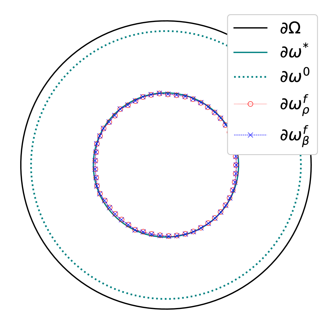
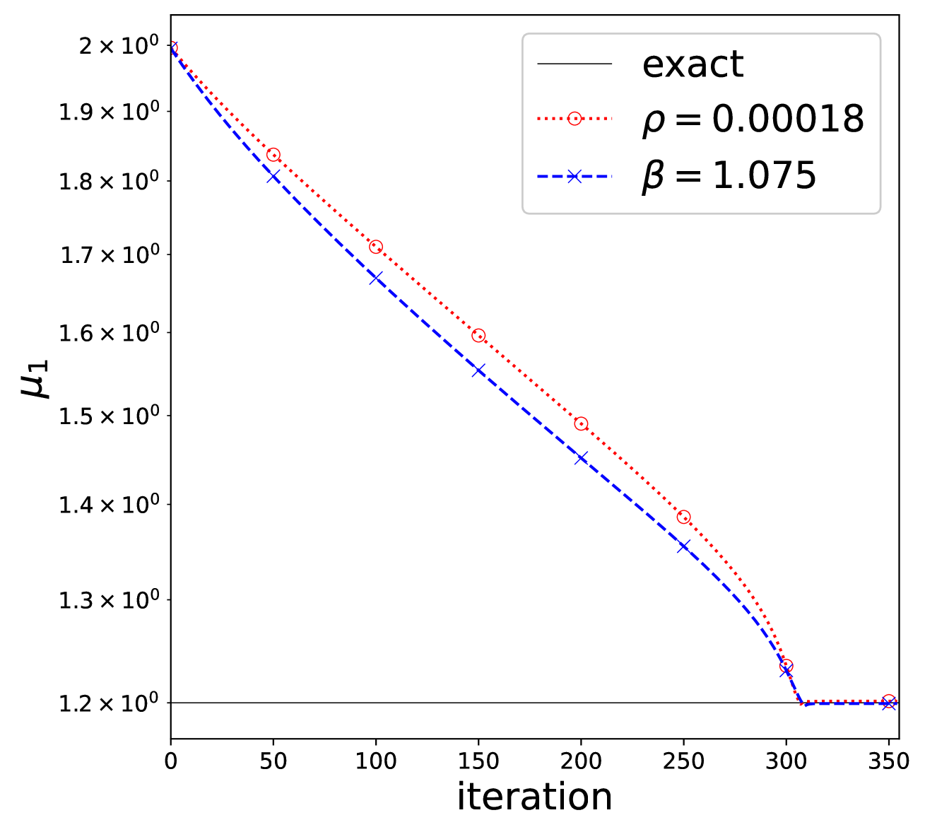
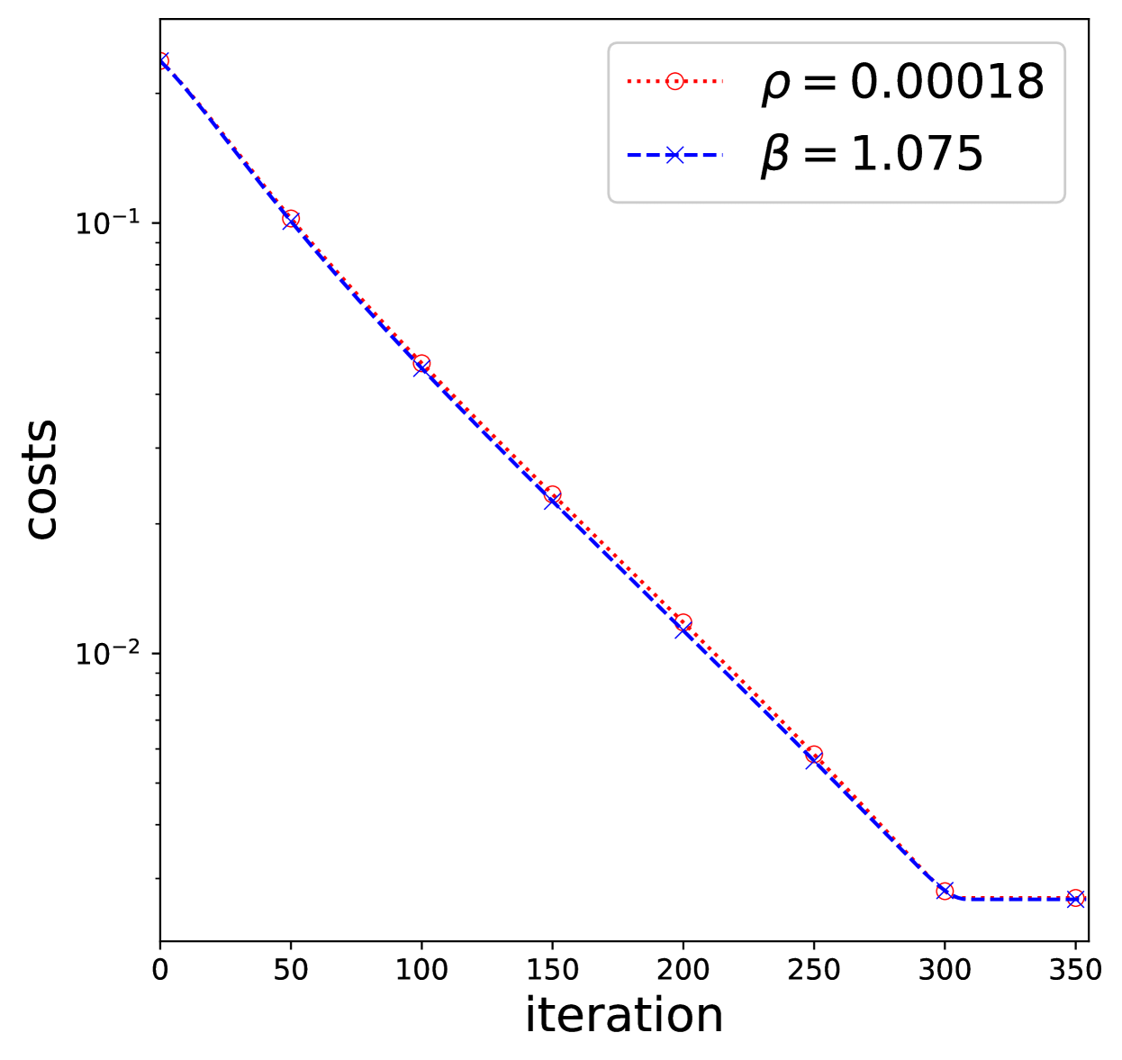
Figure 1. A radial problem in 2D with $\mu_{1}^{\ast}=1.2$ and source function $f=1$

We repeat the experiment with higher values of $\eta^{\ast}$. Using the balancing principle (36), we obtain the results in Figure 2. Accurate identification of $\mu$ and $\partial\omega$ is possible for higher $\eta^{\ast}$ values when an appropriate $\beta$ is chosen with exact measurements.

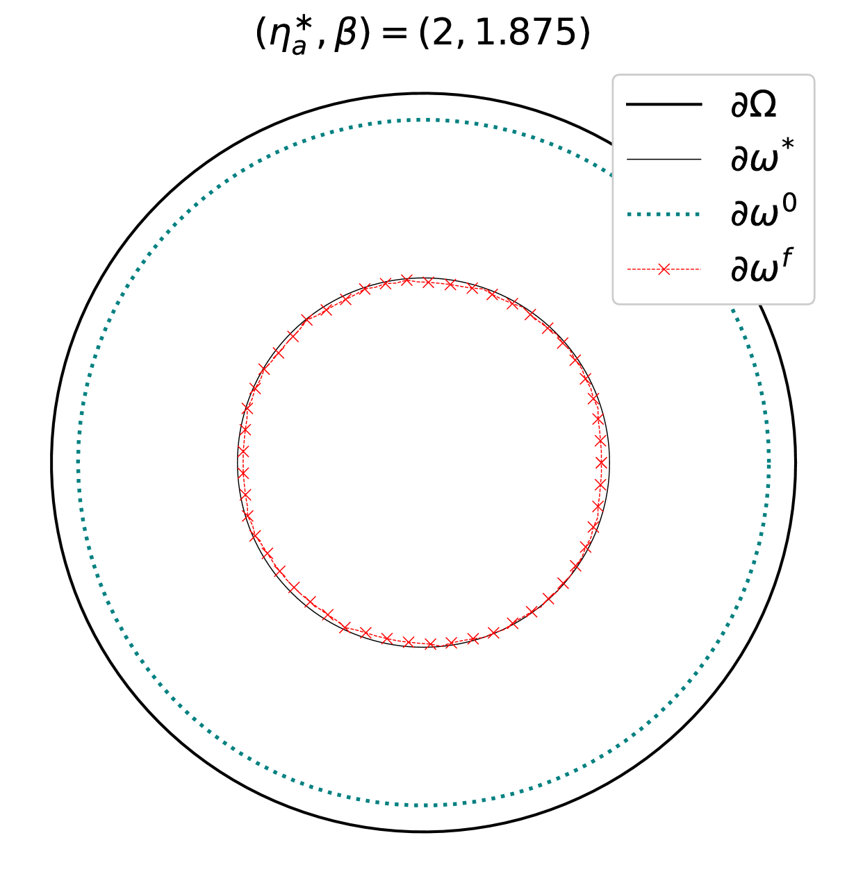
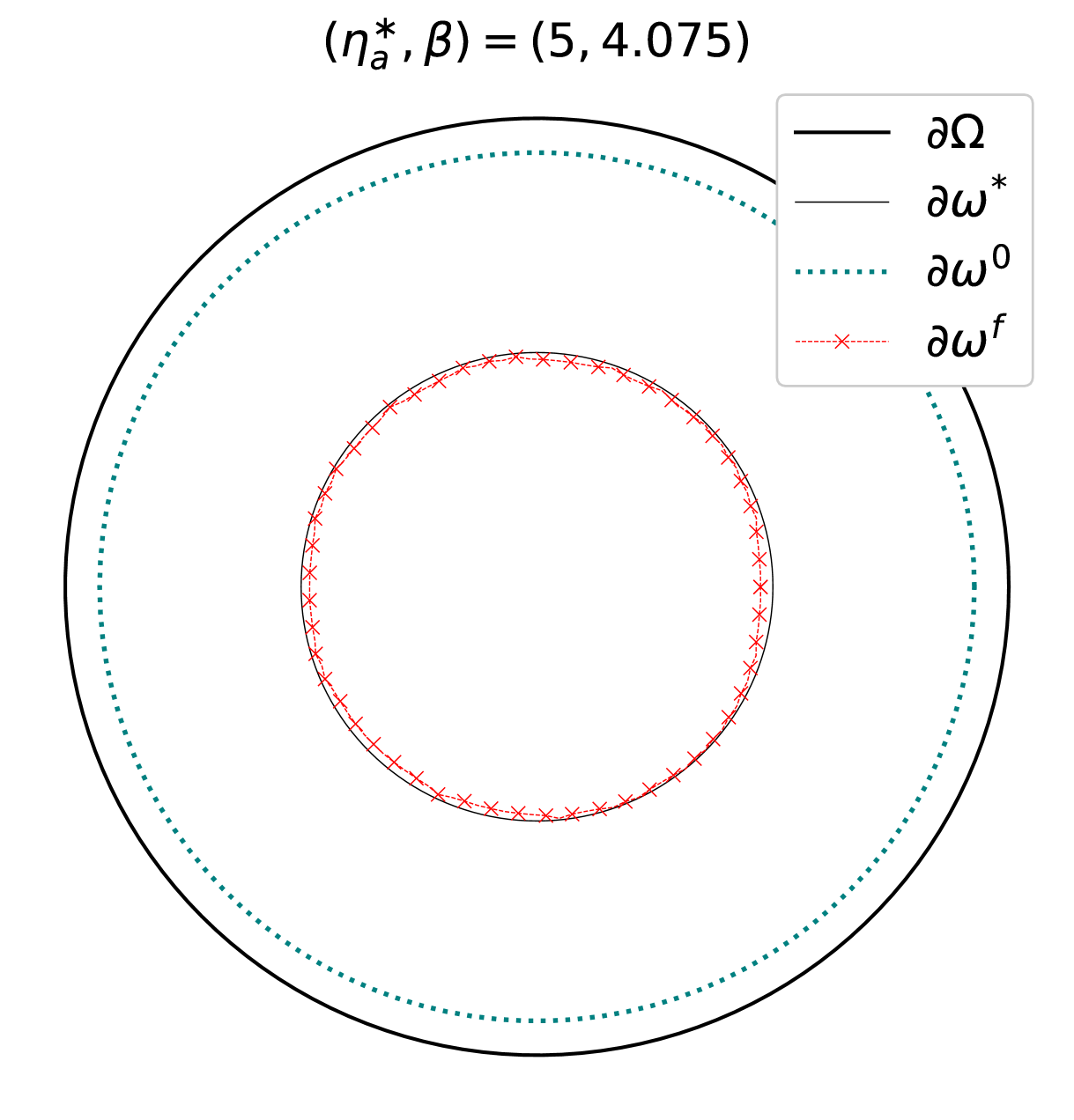
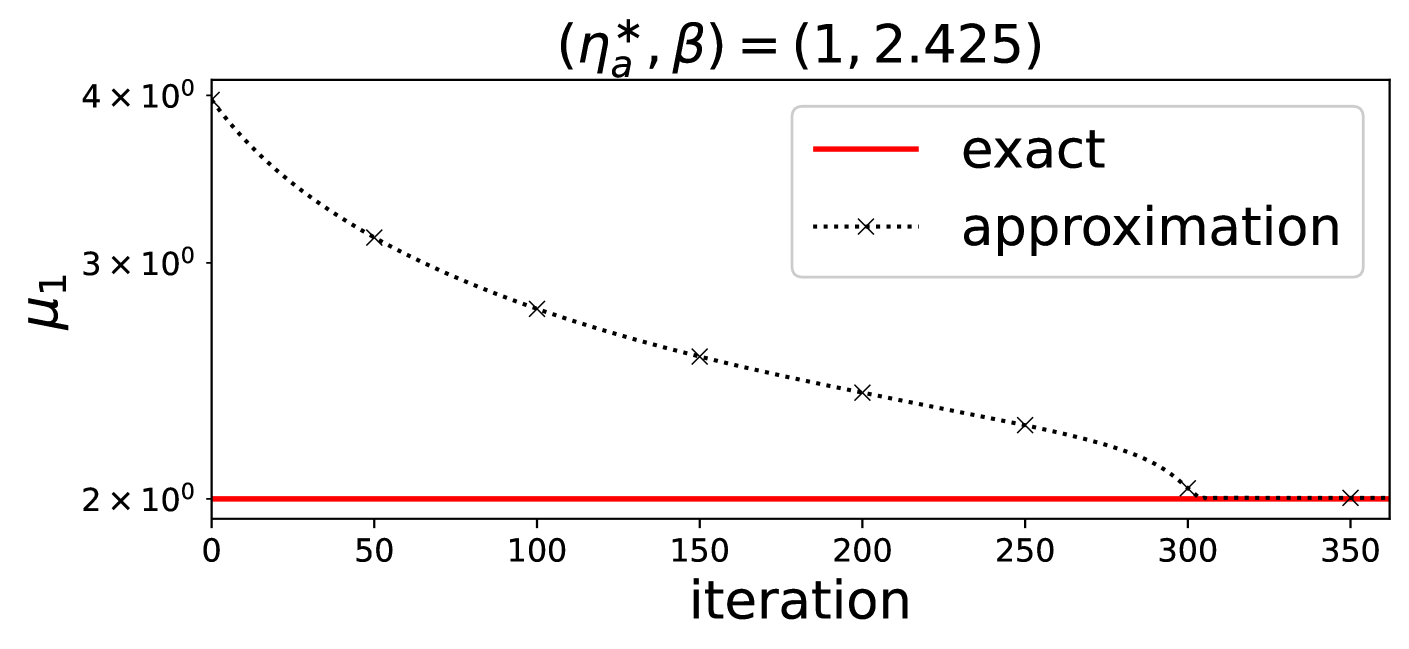
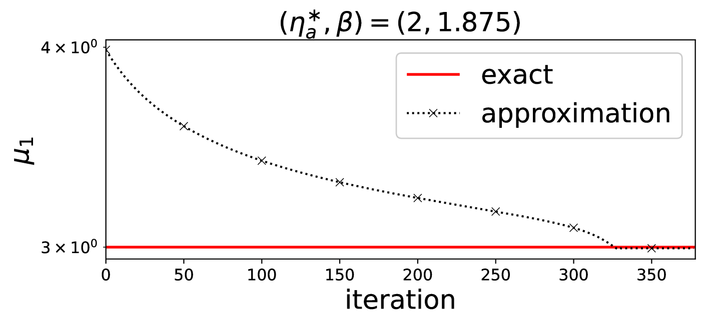
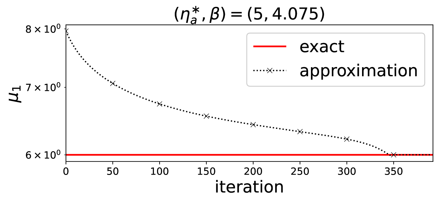
Figure 2. 2D radial problem with source function $f=1$ and varying $\mu_{1}^{\ast}$

4.7. Numerical tests with a point source

We next consider the case of a point source, specifically when $f=\delta(x-x_{0})$, where $x_{0}$ is the position of the point source within $\Omega$. The boundary data for optical tomography can be specified as all possible Cauchy pairs along the boundary. The inverse problem which is considered here is related to fluorescence diffuse optical tomography.

We set $x_{0}=0$ and $(\mu_{0}^{\ast},\mu_{1}^{\ast})=(1,1.2)$. Without applying (36), we obtain the results shown in Figure 3. The leftmost plots correspond to $s=1$, and the middle plots correspond to $s=10$. As expected, increasing the step-size parameter $s$ accelerates convergence toward the exact solution. However, in both cases, the boundary interface approximation is inaccurate. We then repeat the experiment with a new initial guess, $\partial\omega^{0}=B_{0.8}$, yielding a highly accurate approximation of the exact solution, as shown in the rightmost plot of Figure 3. The scheme depends on the initialization, as anticipated. By selecting a good initial guess for $\mu$ and $\partial\omega$, an accurate identification of the unknown coefficient and boundary interface can be achieved.

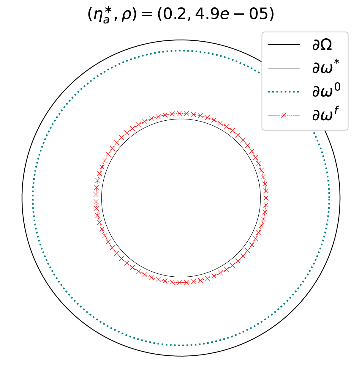
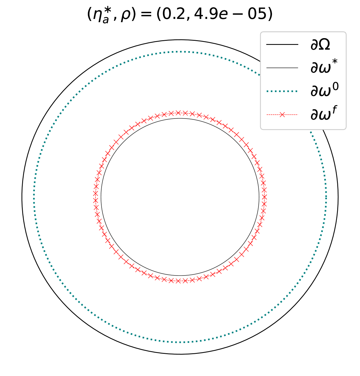
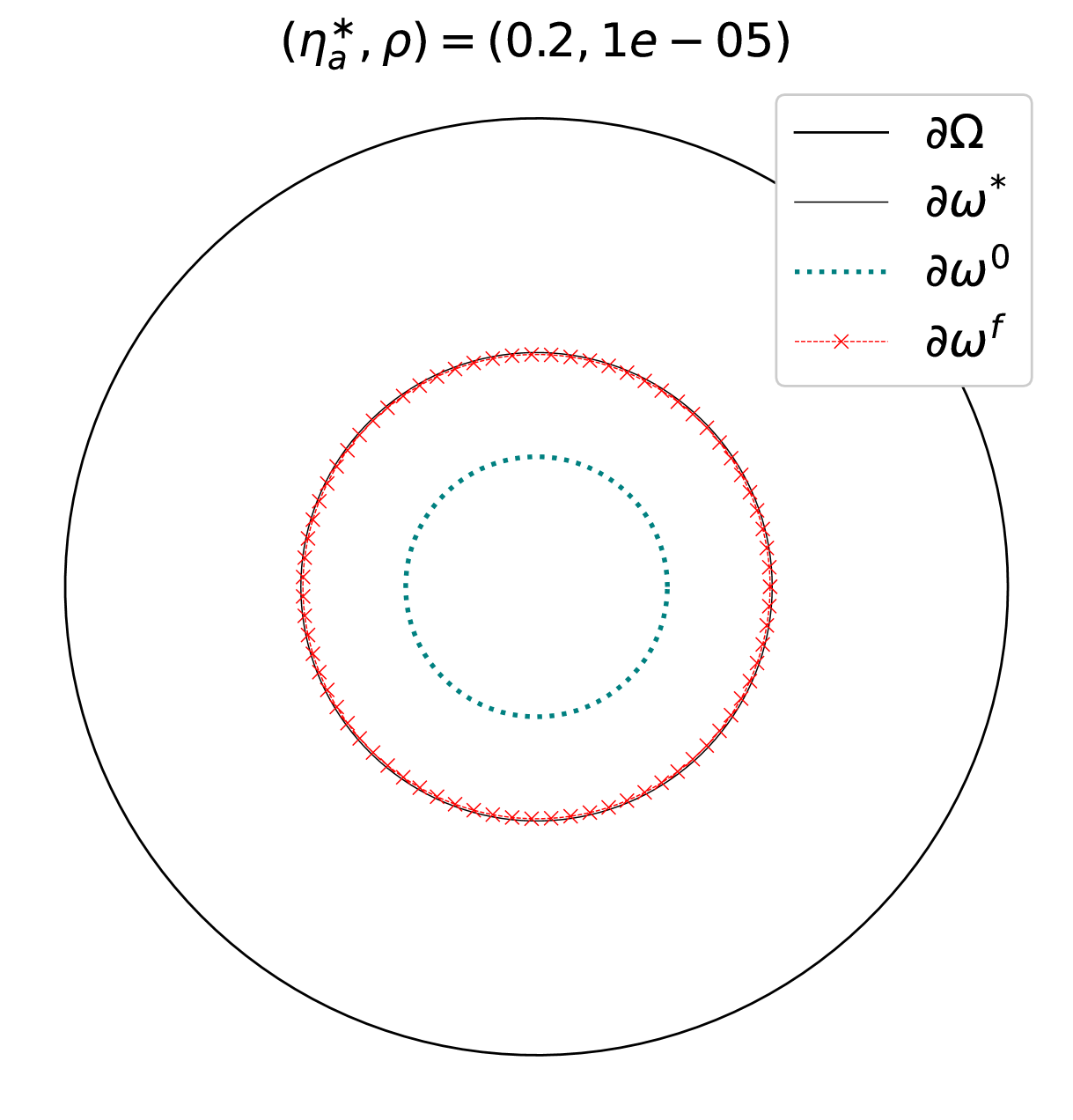
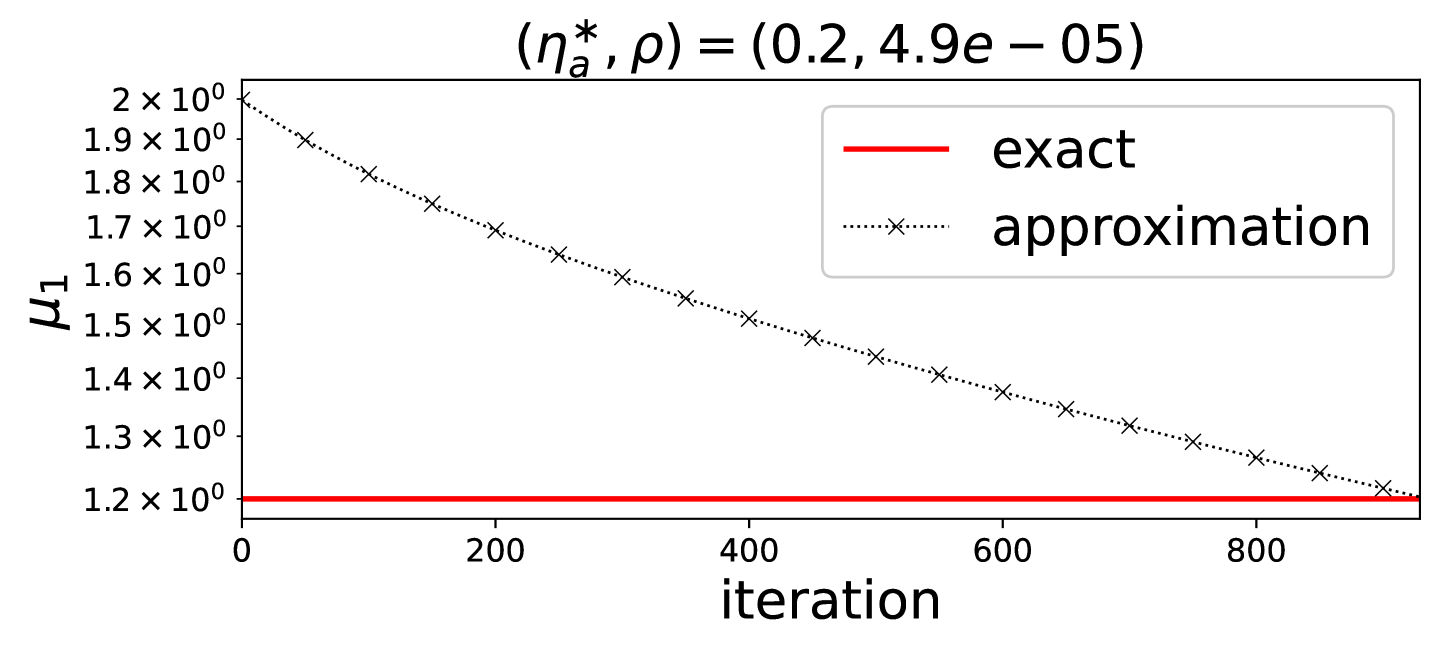
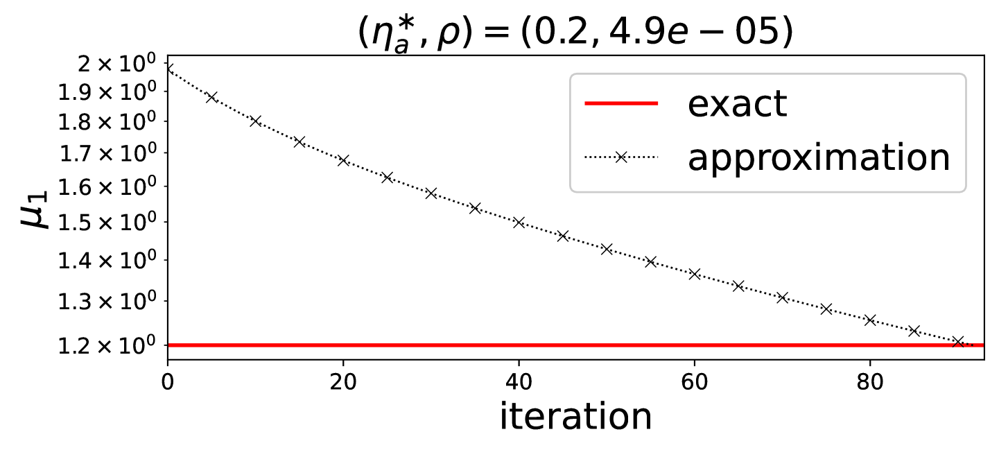
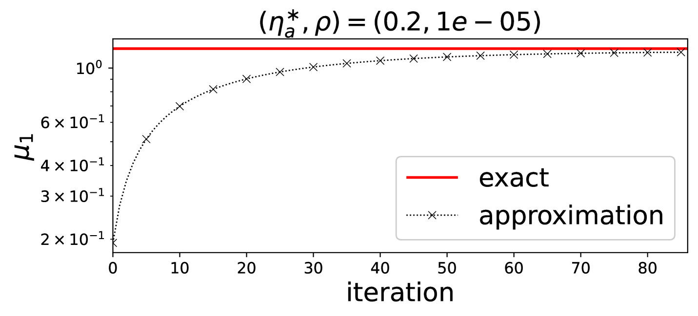
Figure 3. Results for a 2D radial problem with $f(x)=\delta(x)$

We repeat the experiments with slight modifications to $\mu^{\ast}$. Specifically, we examine the main case (38) with varying $\eta^{\ast}=0.2,1,2,5$, but using a point source instead of a spatially oscillating source term. With $s=100$, the results are summarized in Figure (4). By carefully selecting initial guesses for the unknown parameter and boundary interface (see also Figure 3), we achieve precise identification of $\mu$ and $\partial\omega$.

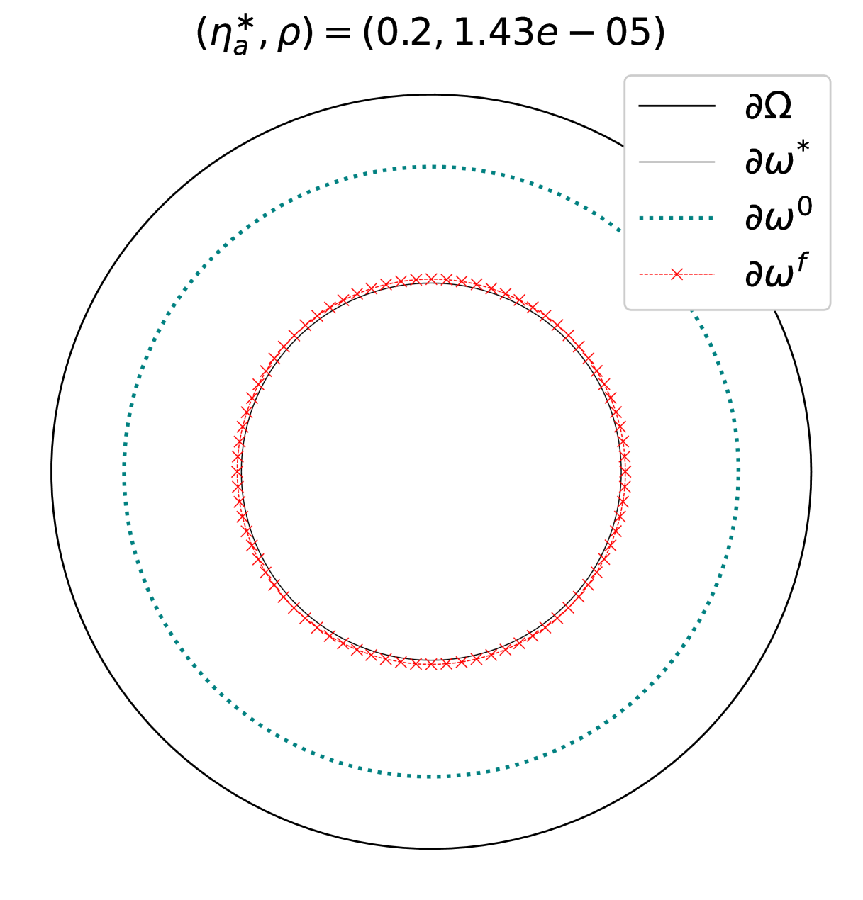
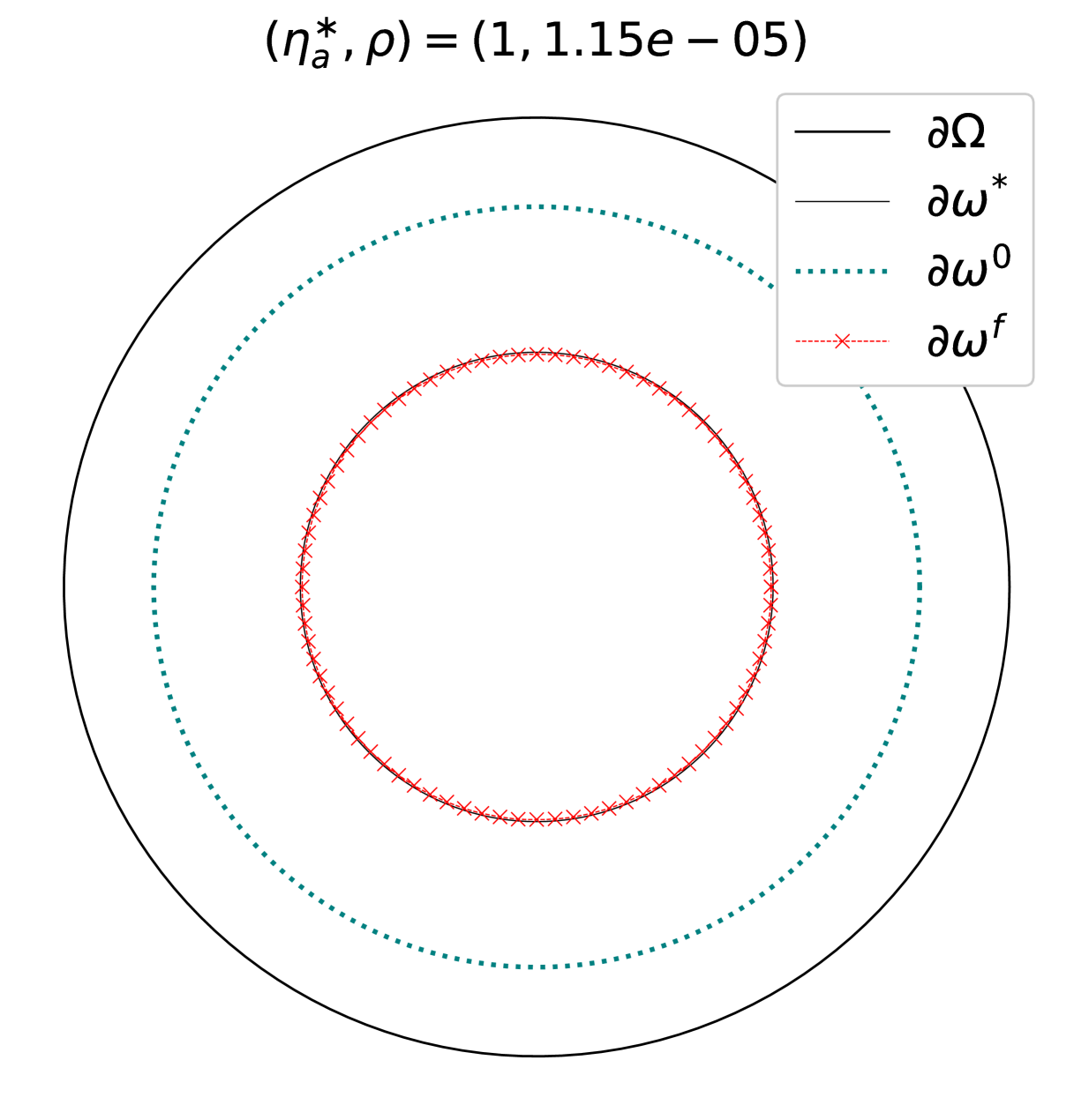
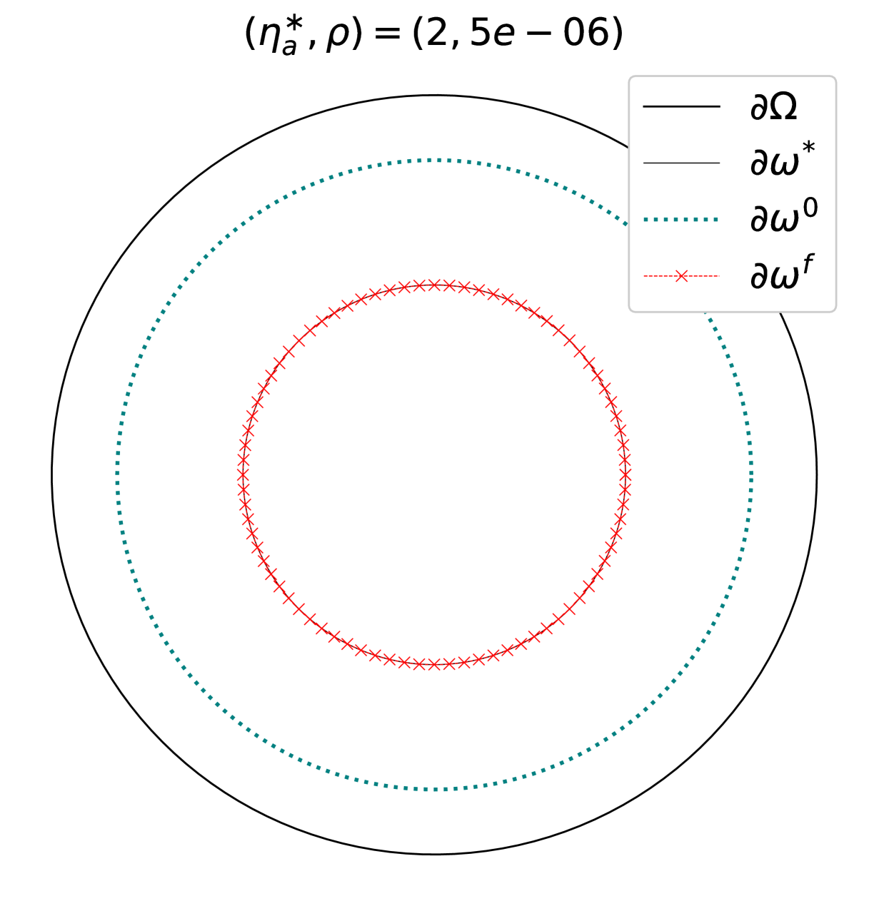
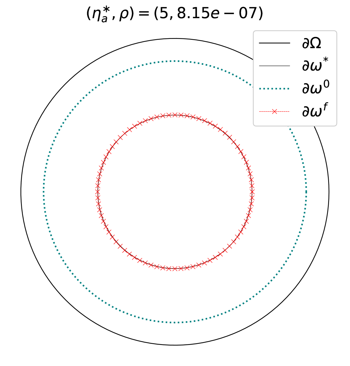
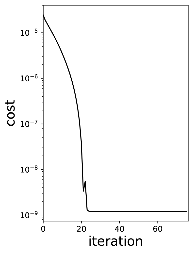
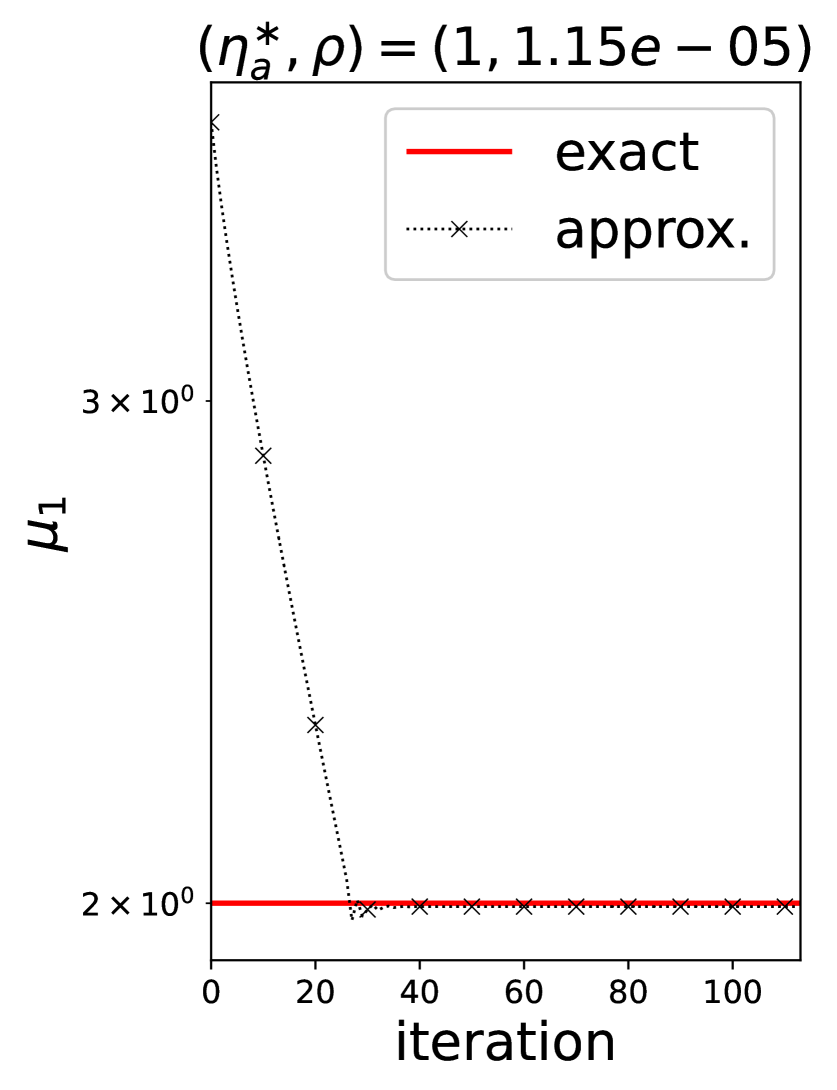
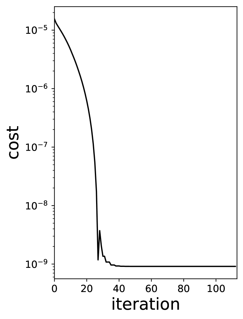
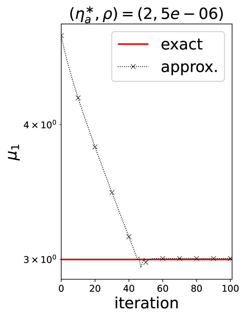
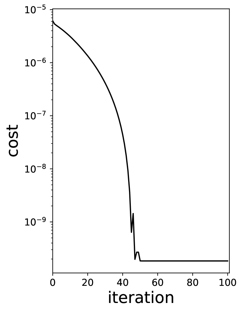
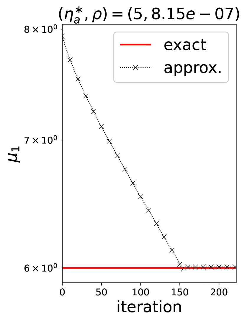
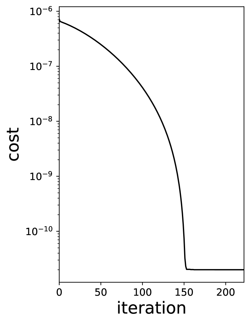
Figure 4. Results for a 2D radial problem with $f(x)=\delta(x)$ and varying $\eta_{a}^{\ast}$

The previous tests were based on precise measurements. For noisy data, we summarize the reconstructions of $\partial\omega^{\ast}=B_{1.5}$ and identifications when $\eta^{\ast}=0.2,5$ in Figure 5. Despite high noise levels, the identifications of both values and shapes were satisfactory. We used the same $\rho$ as in the non-noisy case to demonstrate the impact of noise under a fixed Tikhonov regularization parameter. As expected, the reconstructions were less accurate than with exact measurements, as shown by the cost value history in the rightmost plots of Figure 5. The reconstructions can be improved by adjusting $\rho$.

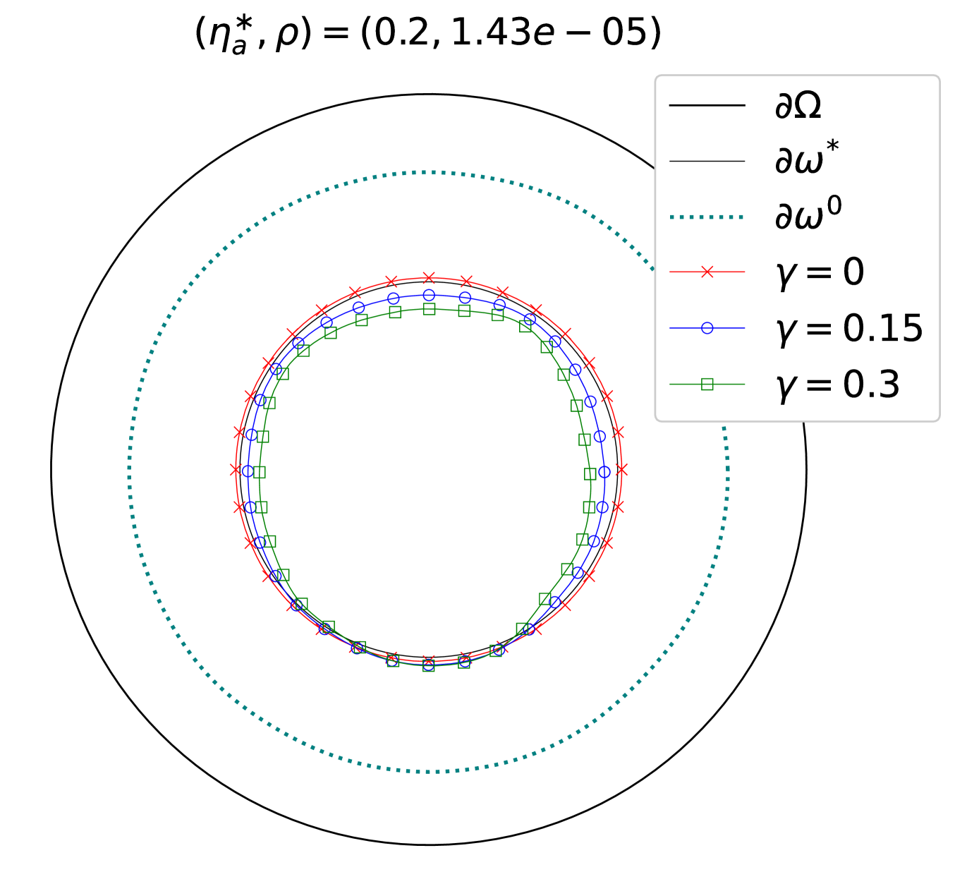
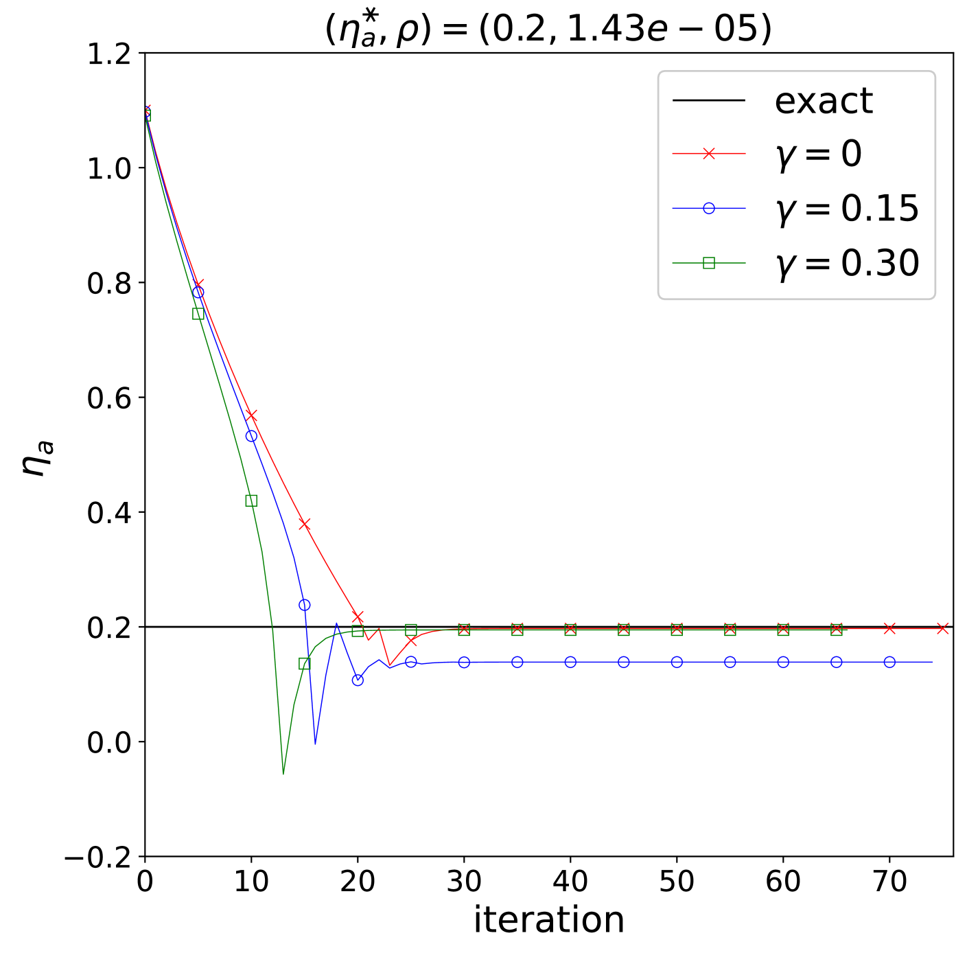
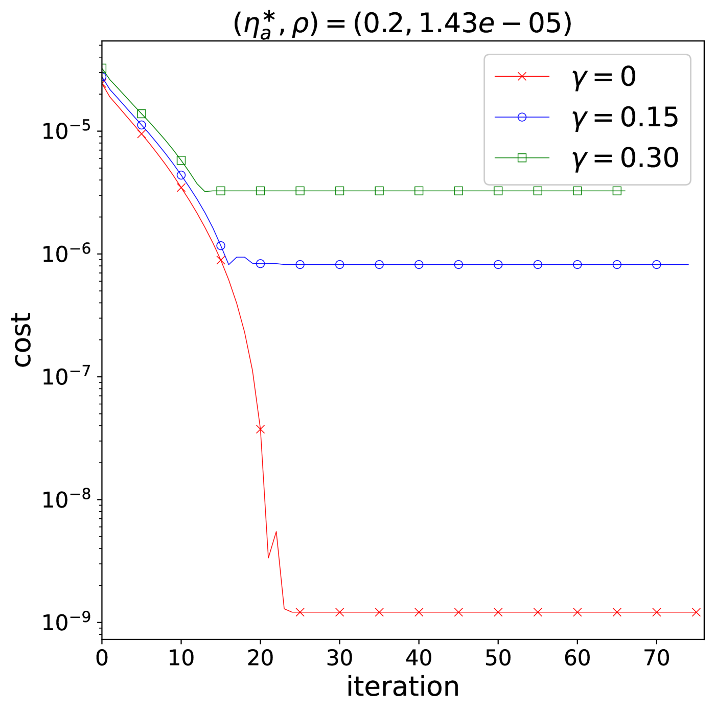
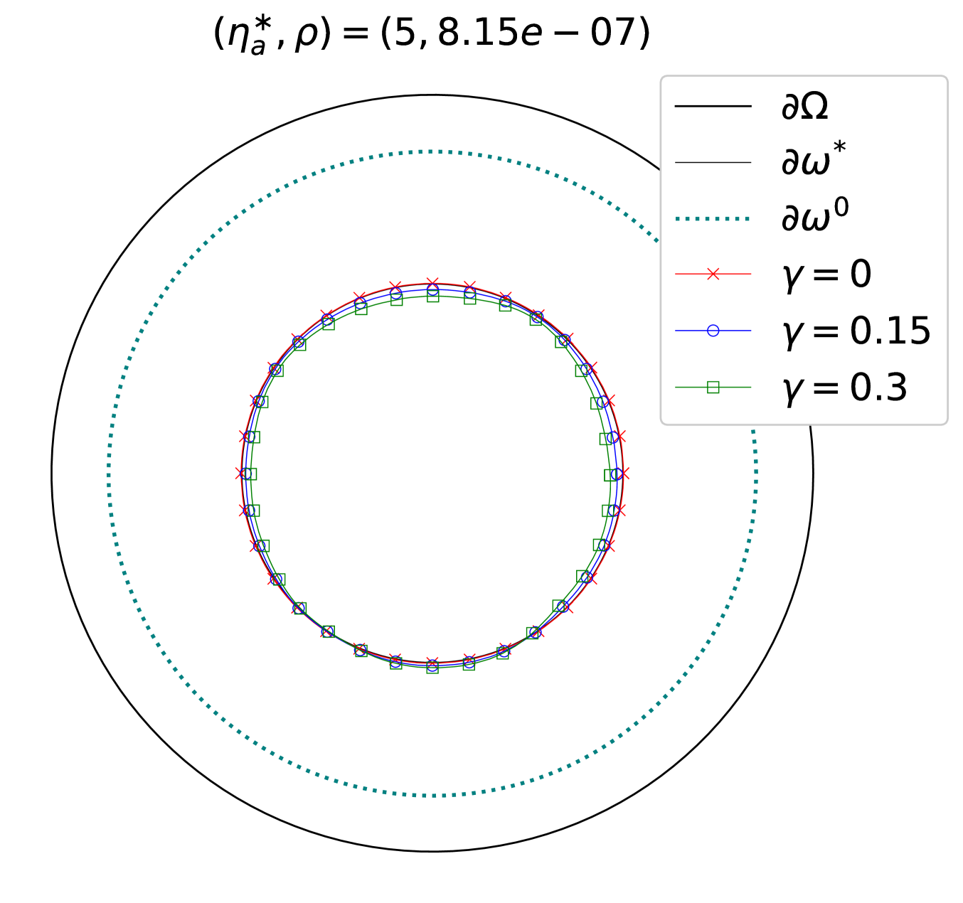
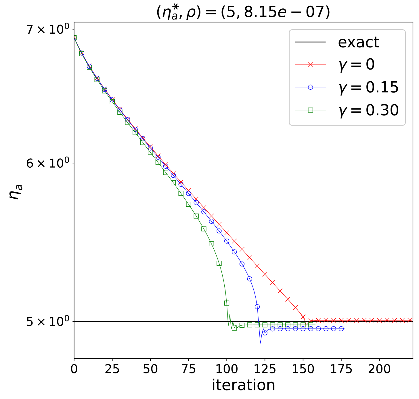
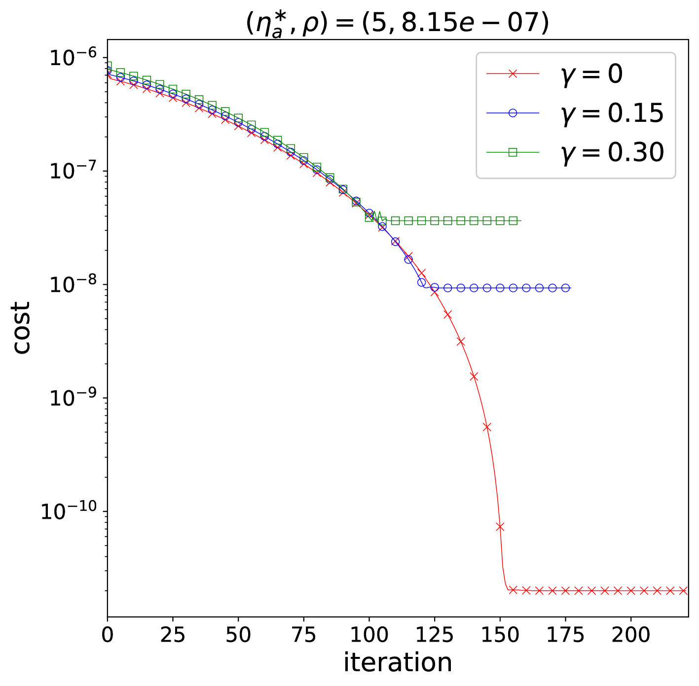
Figure 5. Results for a 2D radial problem with $f(x)=\delta(x)$ under noisy data, with $\eta^{\ast}=0.2$ (left three plots) and $\eta^{\ast}=5$ (right three plots)

4.8. Numerical tests with a constant source function and non-circular boundary interface

We repeat the experiments from subsection 4.6, but with the exact boundary interface given by:

$$\partial\omega^{\ast}=\left\{5(0.4+0.06\cos(3t))\begin{pmatrix}\cos{t}\\ \sin{t}\end{pmatrix},\forall t\in[0,2\pi)\right\}.$$

This boundary is non-convex with minor concavities. As before, we set $f=1$, $k=1$, $R=3$, and $l=0.3$, and show the results for $\eta_{a}^{\ast}=0.2$ in Figures 6 with $\rho=0.0002$ and $s=4$. Though the reconstruction misses the concavities, it closely matches the exact boundary, and the method accurately identifies $\mu_{1}$.

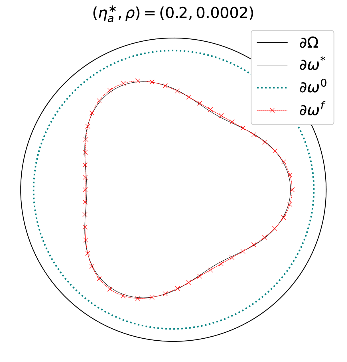
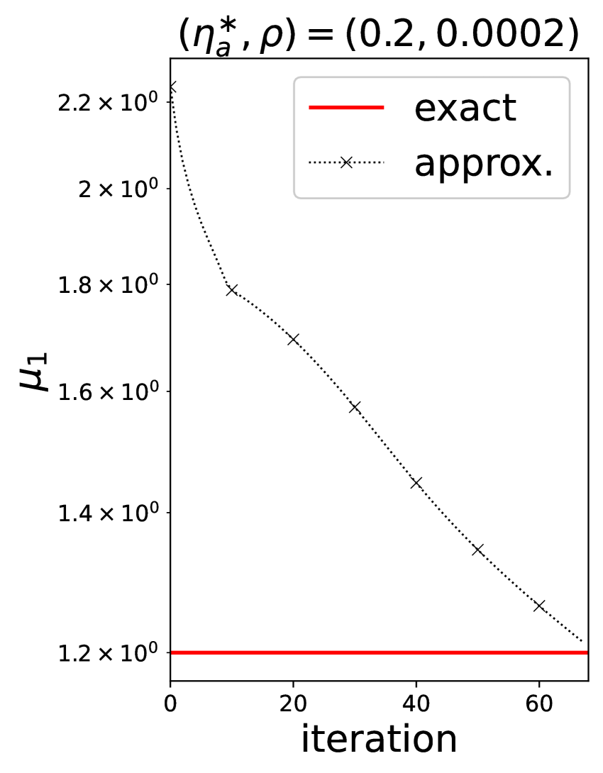
Figure 6. An example featuring a non-circular boundary interface

We perform another set of experiments with noisy data at two different levels. The numerical results, displayed in Figures 7, show the results when $\gamma=0.5,0.10$. As expected, the reconstructions are less accurate compared to those with exact measurements but are still reasonable, as seen in the figures. The relative errors of the computed absorption coefficient and boundary interface are close to the specified noise levels.

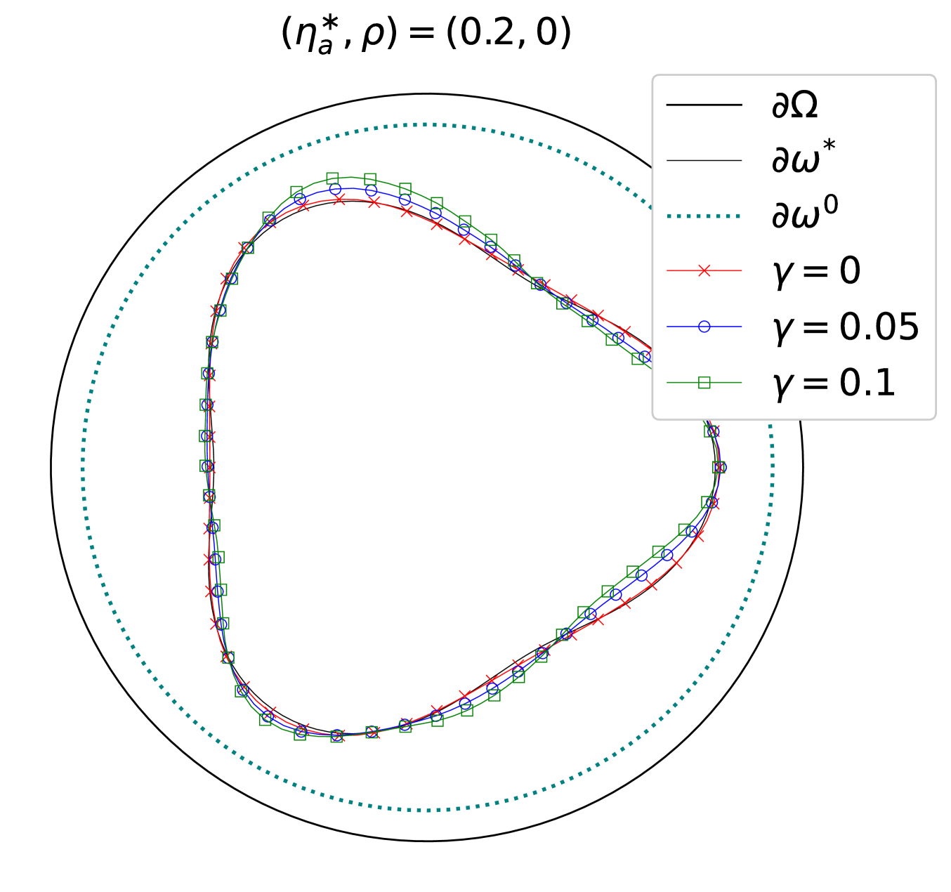
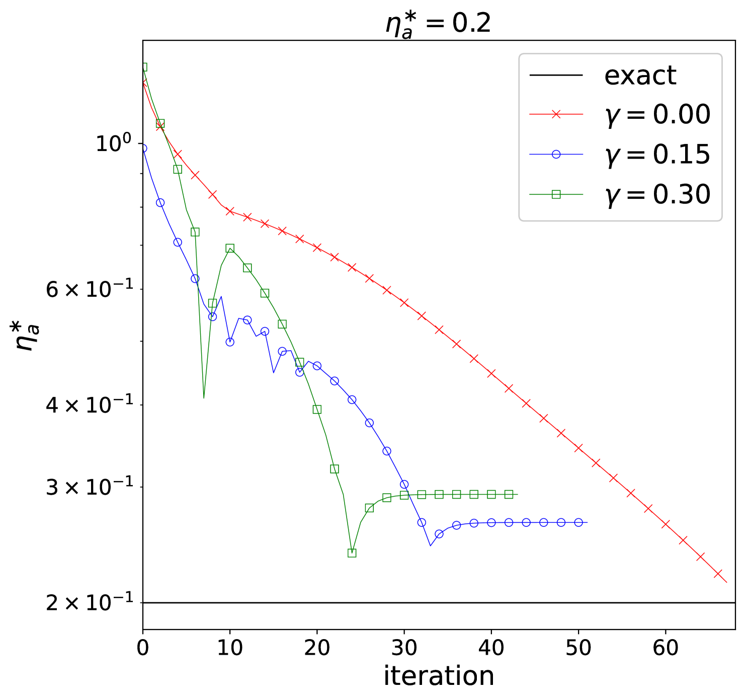
Figure 7. An example featuring a non-circular boundary interface with noisy data

Next, we conduct experiments by varying $\eta_{a}^{\ast}$ with exact measurements, where the initial guess is smaller than the exact boundary interface and positioned inside $\partial\omega^{\ast}$. Specifically, we use $\partial\omega^{0}=B_{0.5}$ as the initial boundary geometry and set $s=10$. The results, including the histories of $\mu_{1}$ and cost values, are shown in Figure 8. The method successfully identified the boundary interface, including its concave parts, and the values for $\mu_{1}$ closely match the exact values, demonstrating the approach’s robustness.

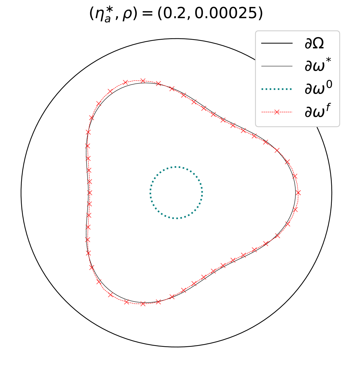
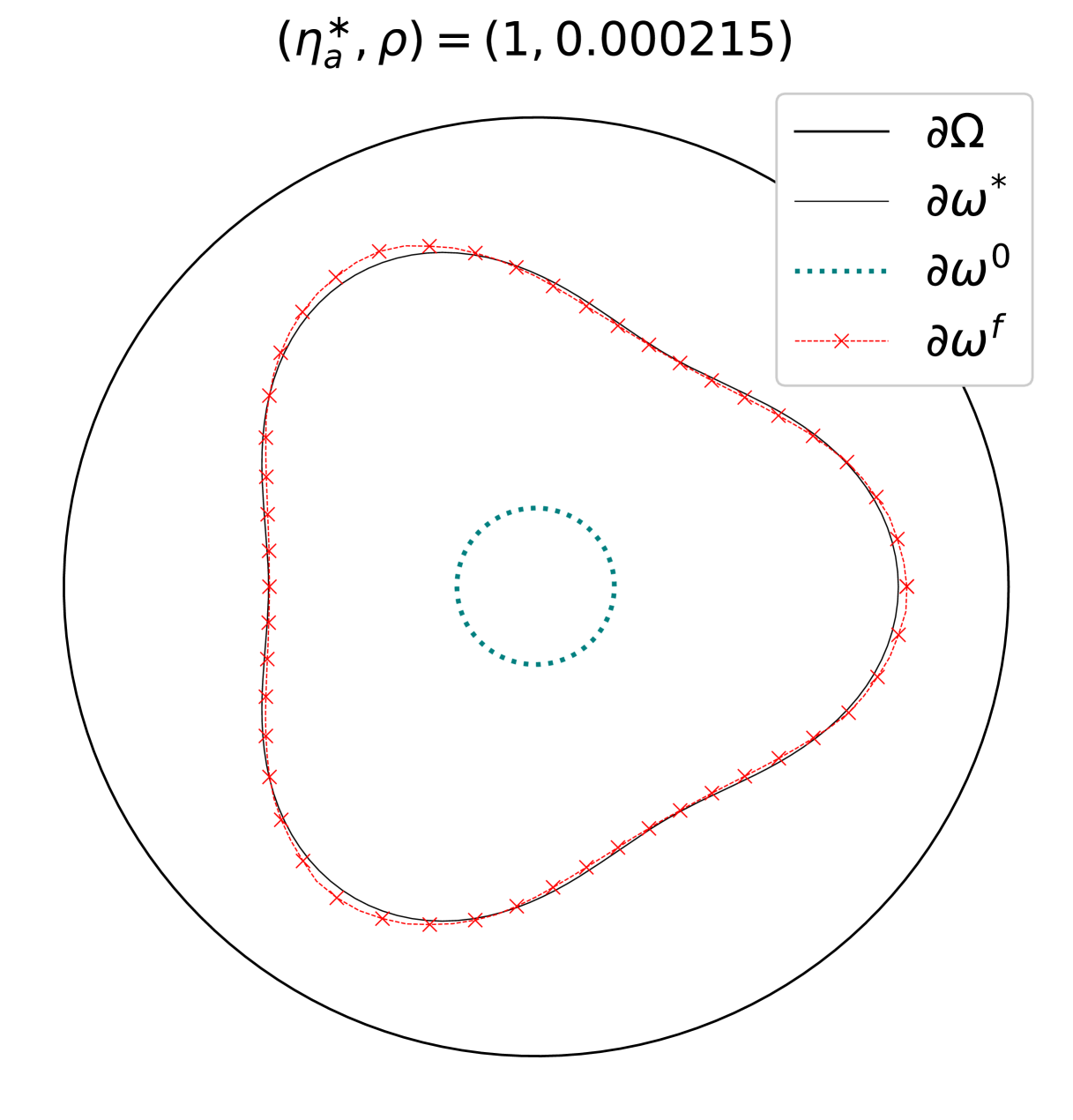
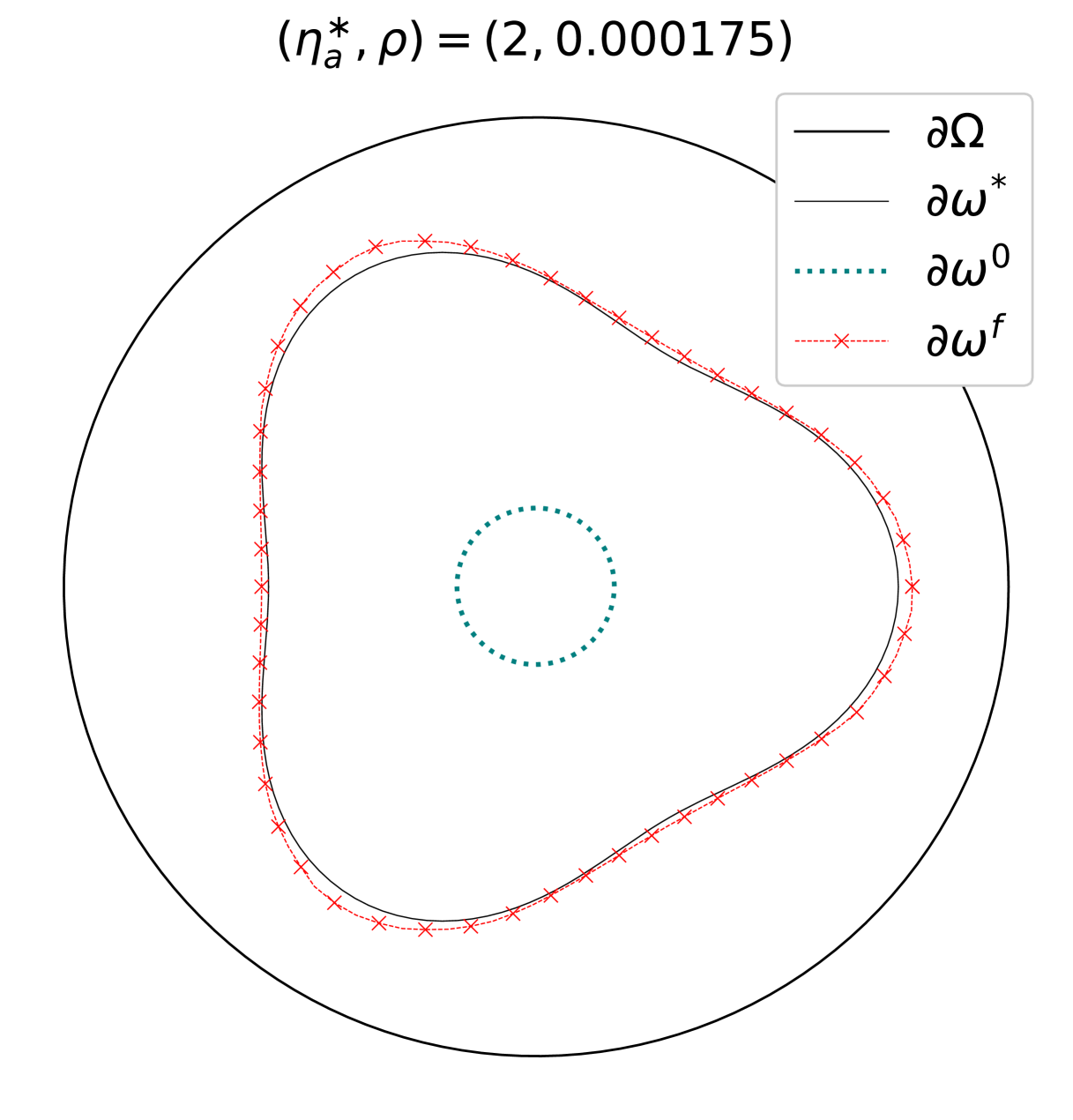
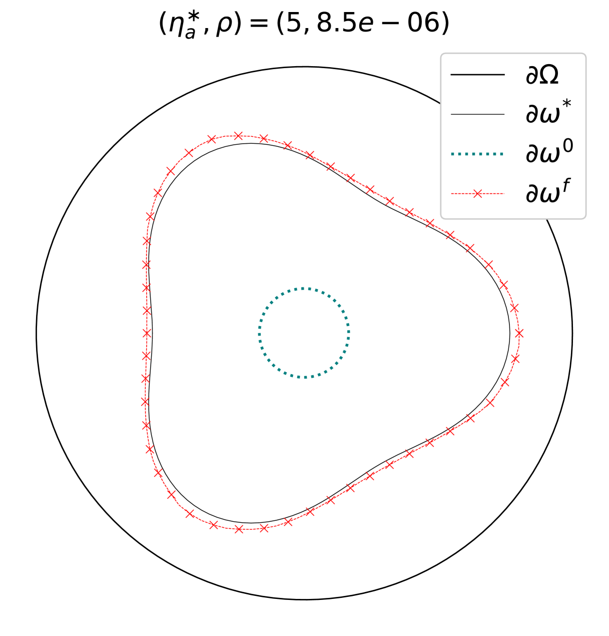
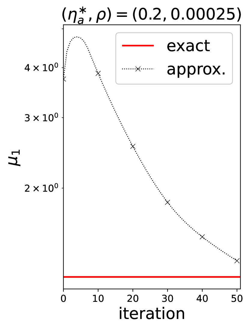
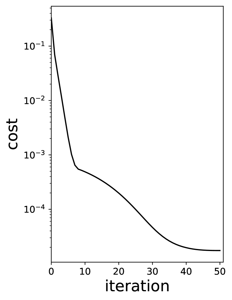
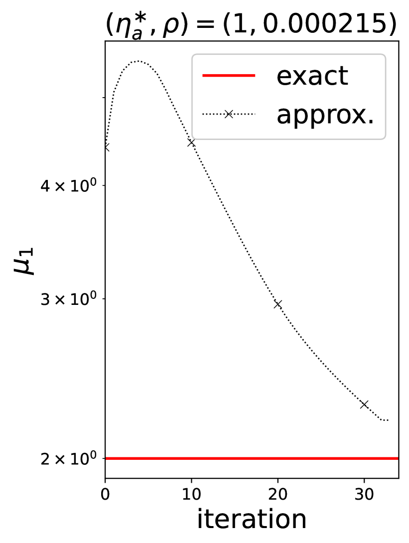
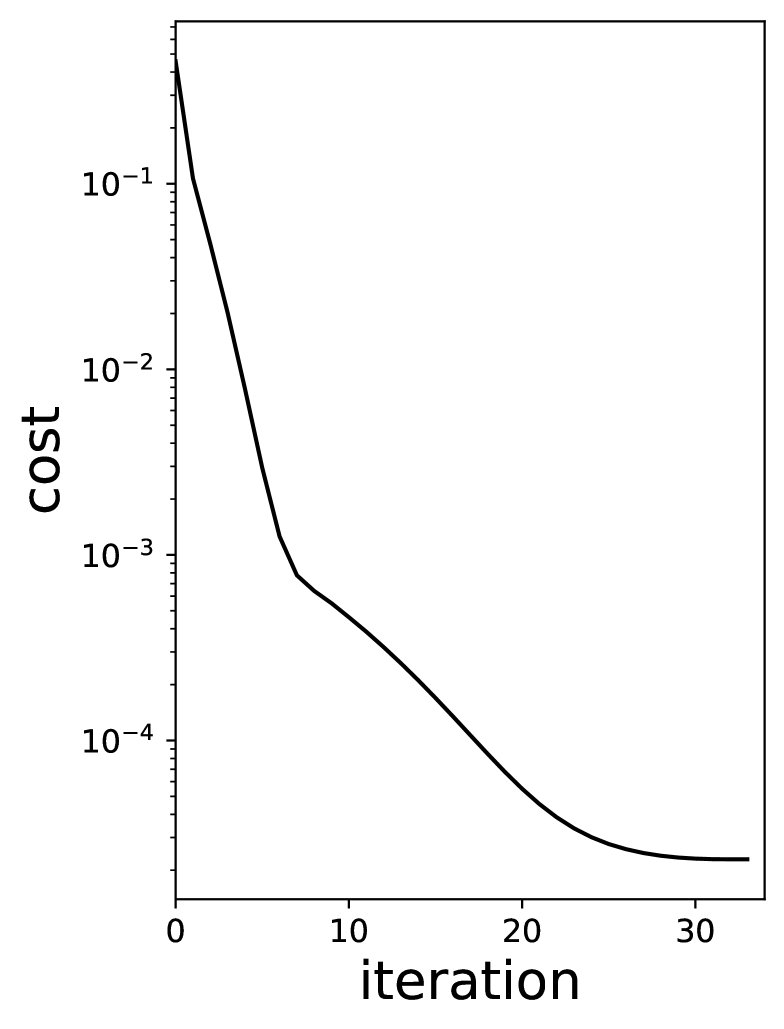
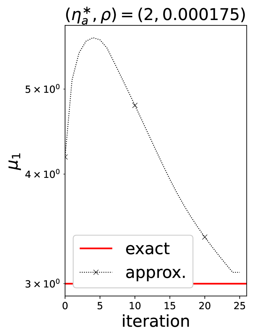
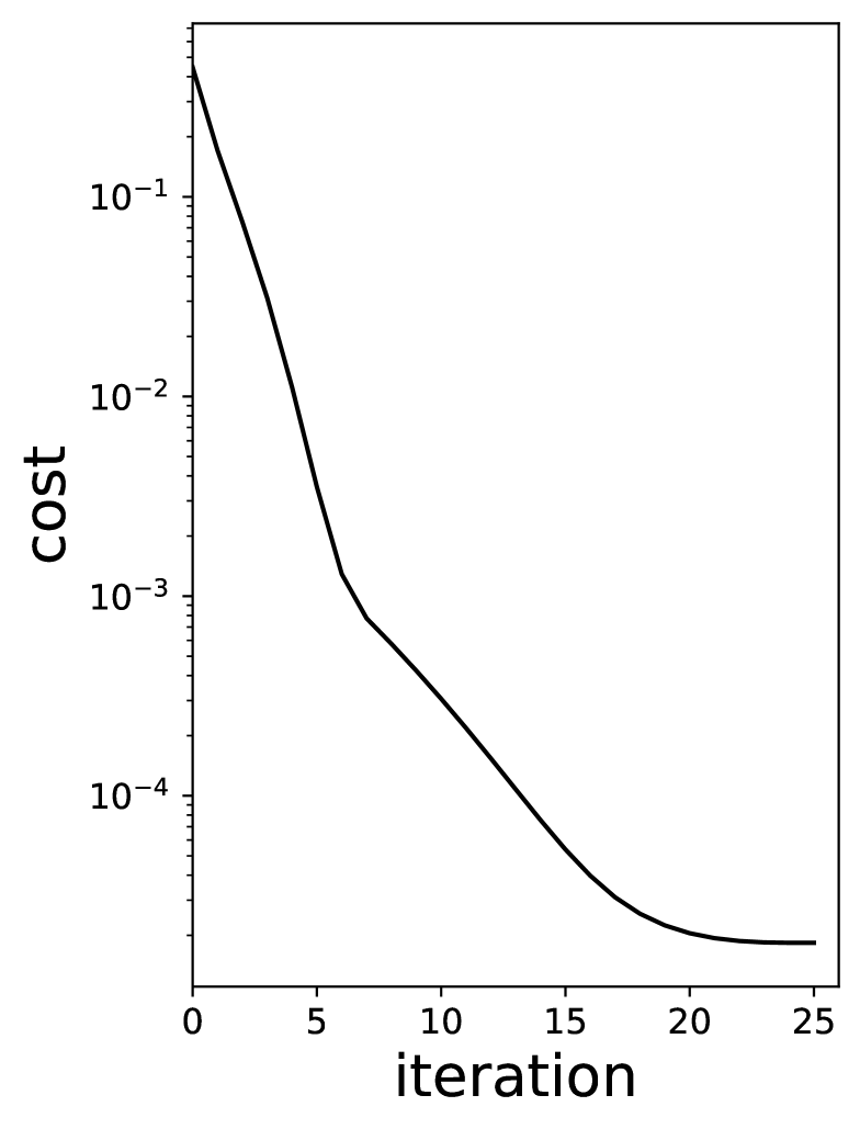
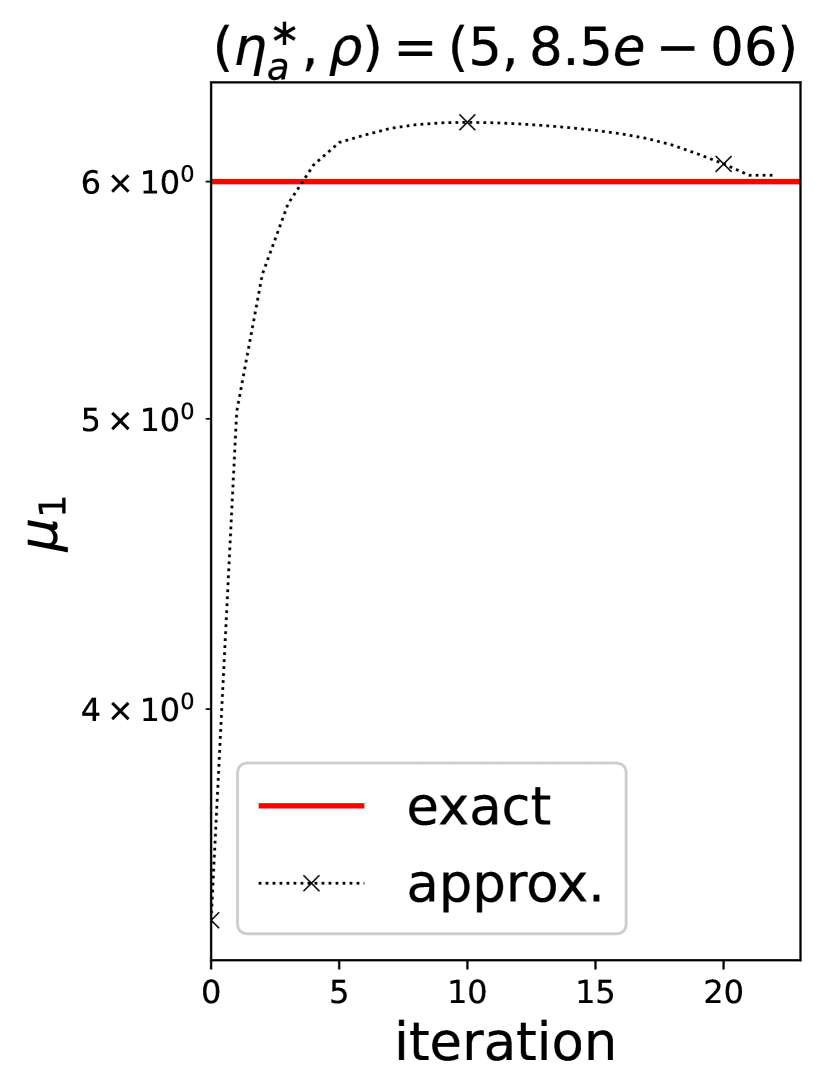
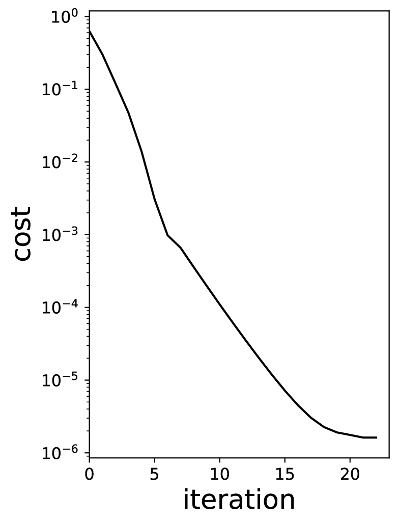
Figure 8. Results for a non-circular boundary interface with varying $\eta_{a}^{\ast}$ values

For the reconstruction with noisy data at $\gamma=0.05,0.10$ and $\eta^{\ast}=5$, the results are shown in Figure 9. The Tikhonov regularization parameter $\rho$ is chosen based on the noise level, and a large step-size parameter $s=5$ is used. Despite the noise, the method successfully reconstructed the boundary interface and identified the absorption coefficient with good accuracy. The histories of $\mu_{1}$ and the cost are also shown, with higher noise levels corresponding to larger cost values.

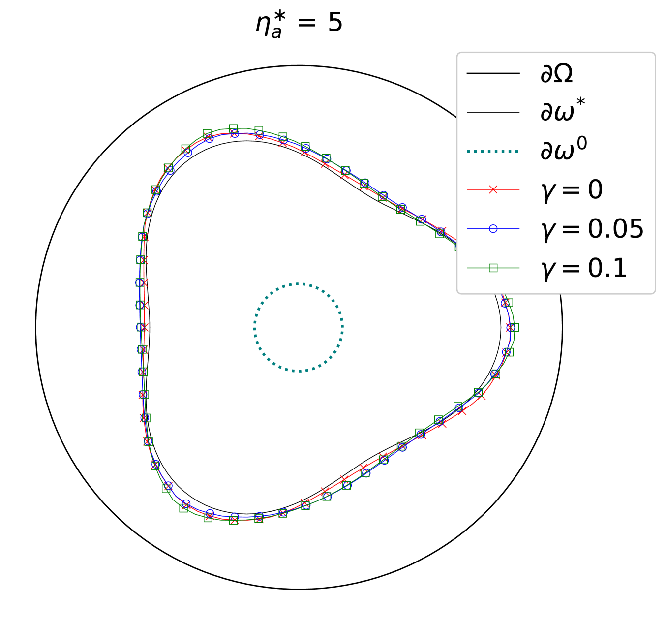
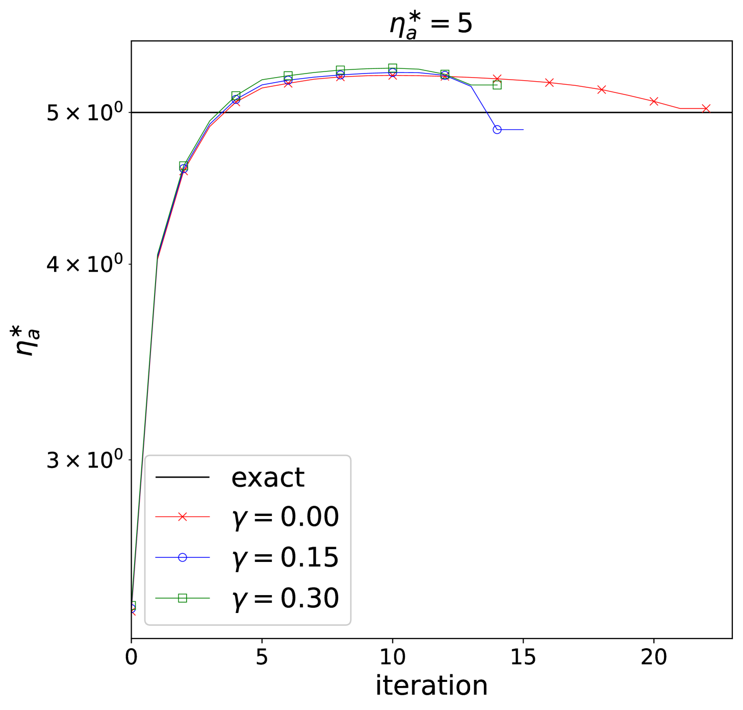
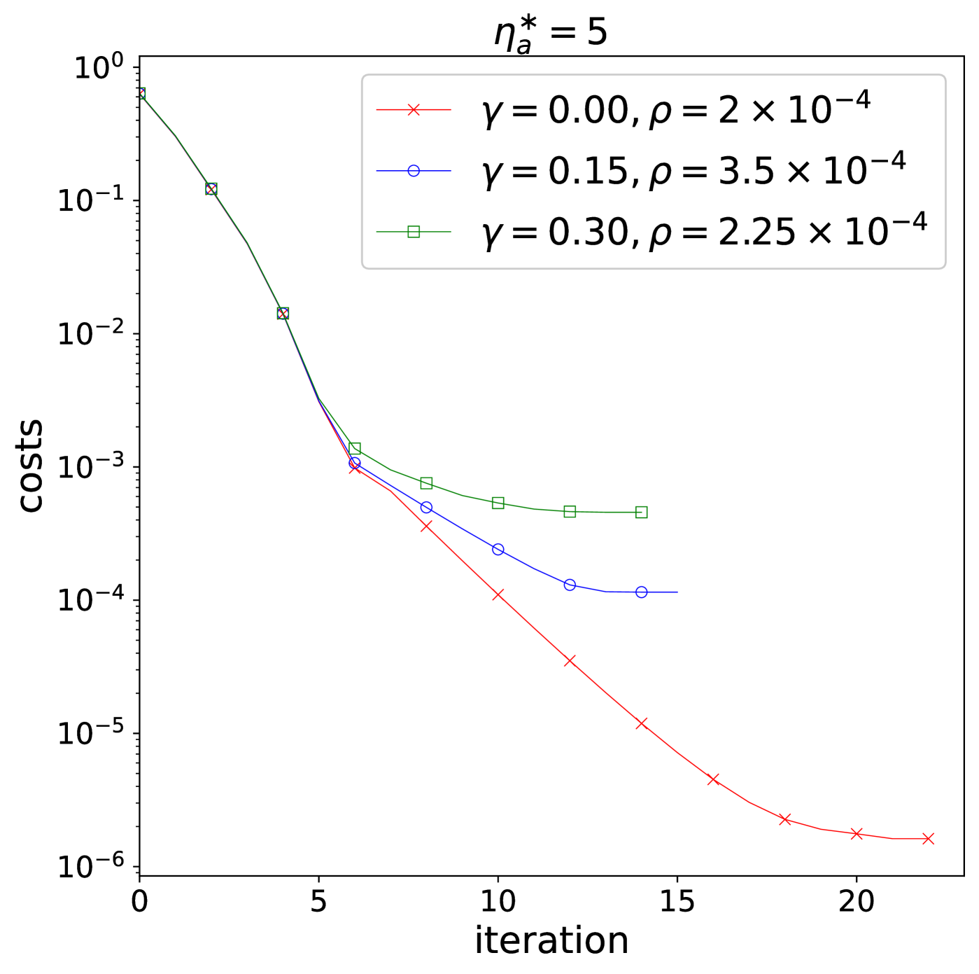
Figure 9. An example featuring a non-circular boundary interface with noisy data

We repeated the experiment using a peanut-shaped boundary interface and fixed $\rho$ at 0.0001. The results, shown in Figure 10, demonstrate that despite the complex shape, the recovery of the absorption coefficient and boundary geometry remained accurate, even with high noise. This highlights the robustness of the method for constant source.

To further assess robustness, we examined the impact of different initial guesses with noisy data at $\gamma=0.10$. As shown in Figure 11, the reconstruction accuracy depends on the initial shape position, as expected. However, the reconstruction converged to an almost identical exact shape, even under high noise. Similar results can be expected with varying initial shape geometries.

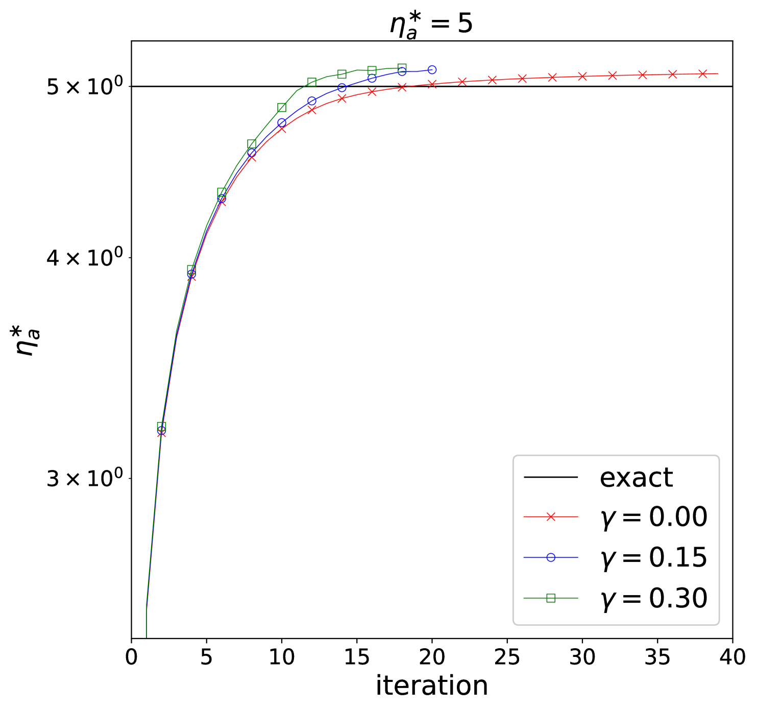
Figure 10. An example of a peanut-shaped boundary interface with noisy data

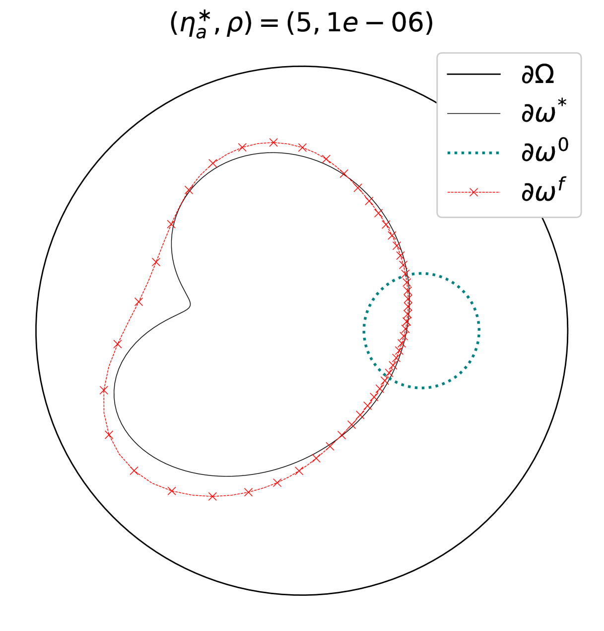
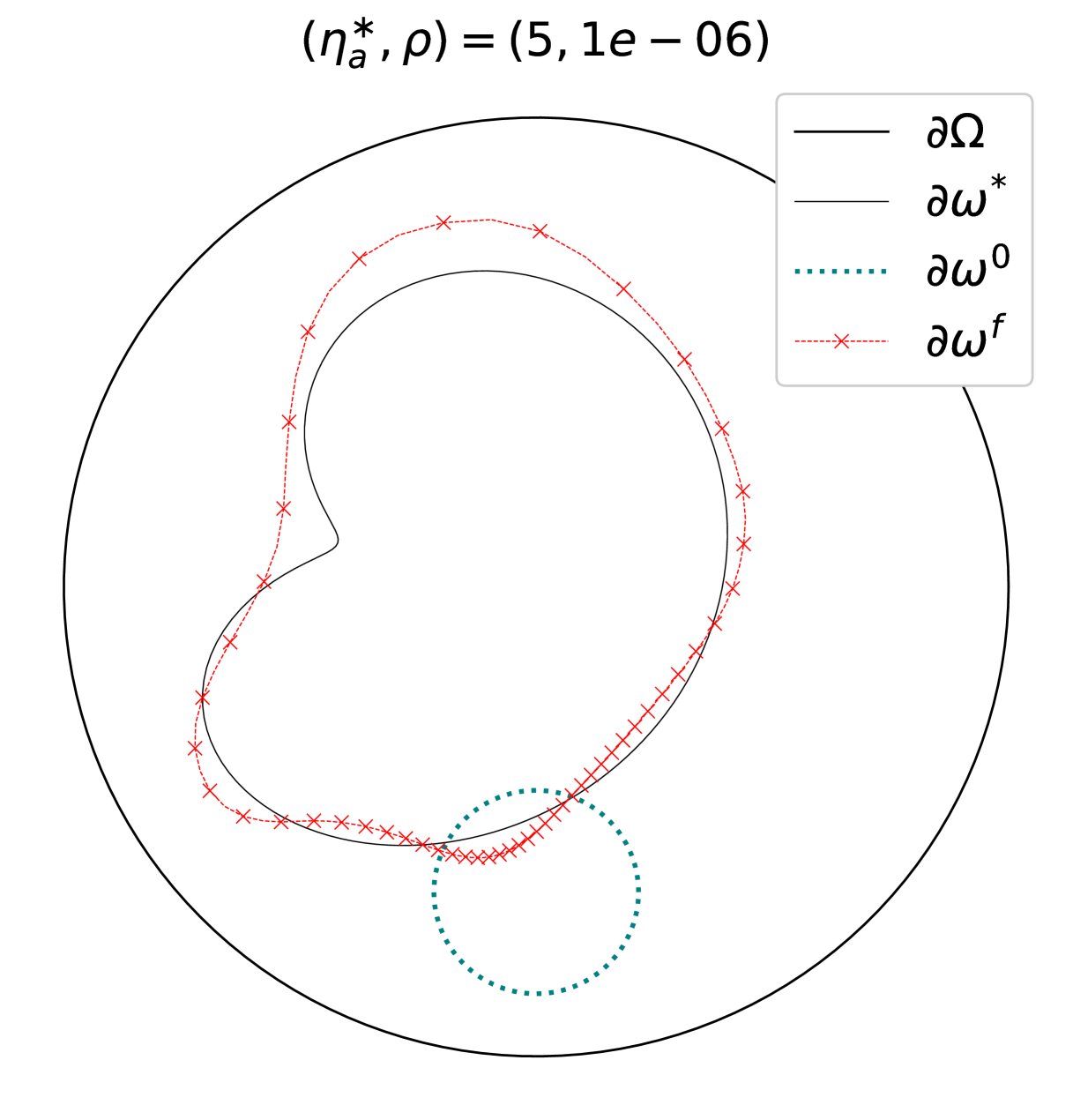
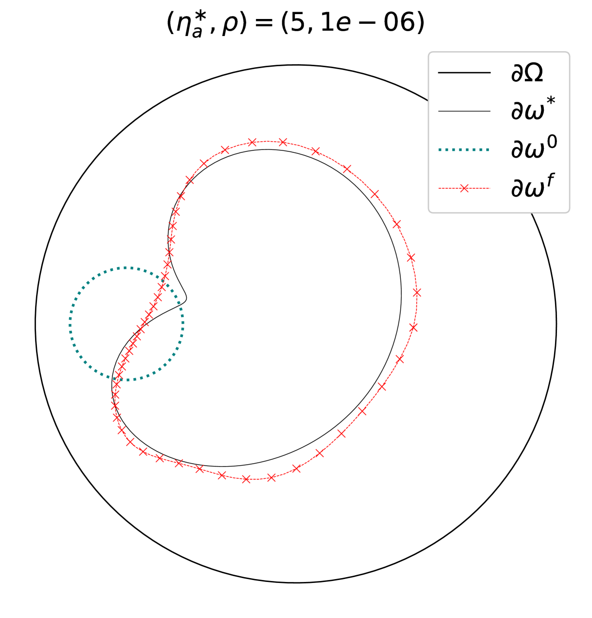
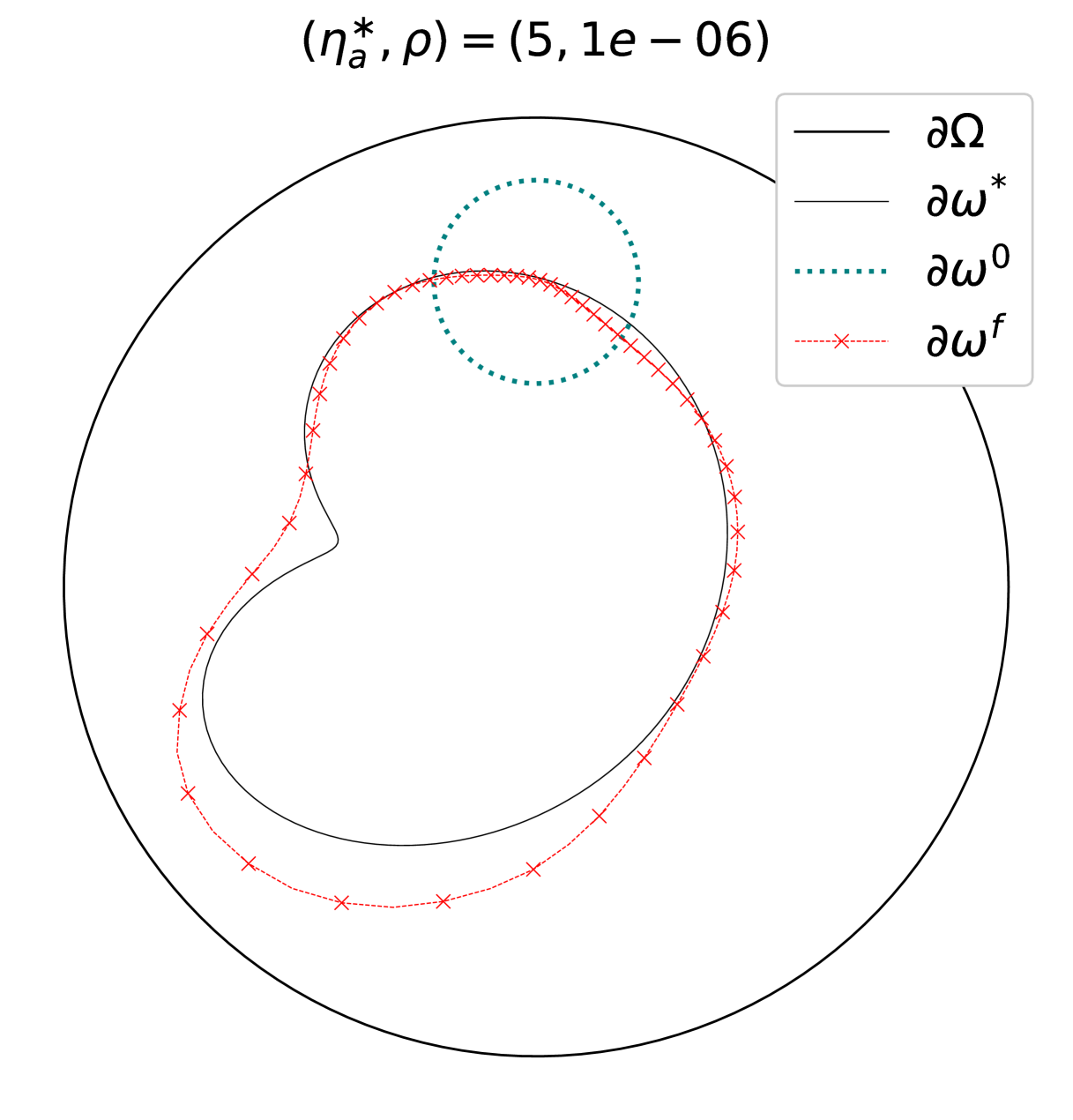
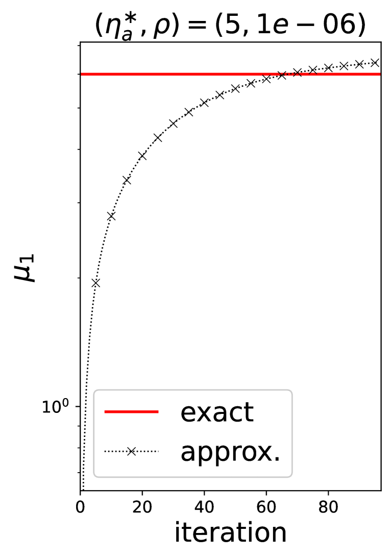
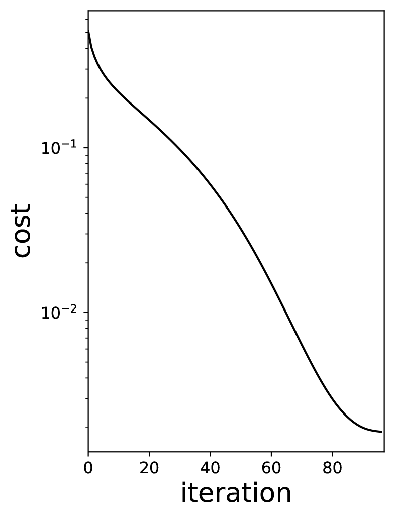
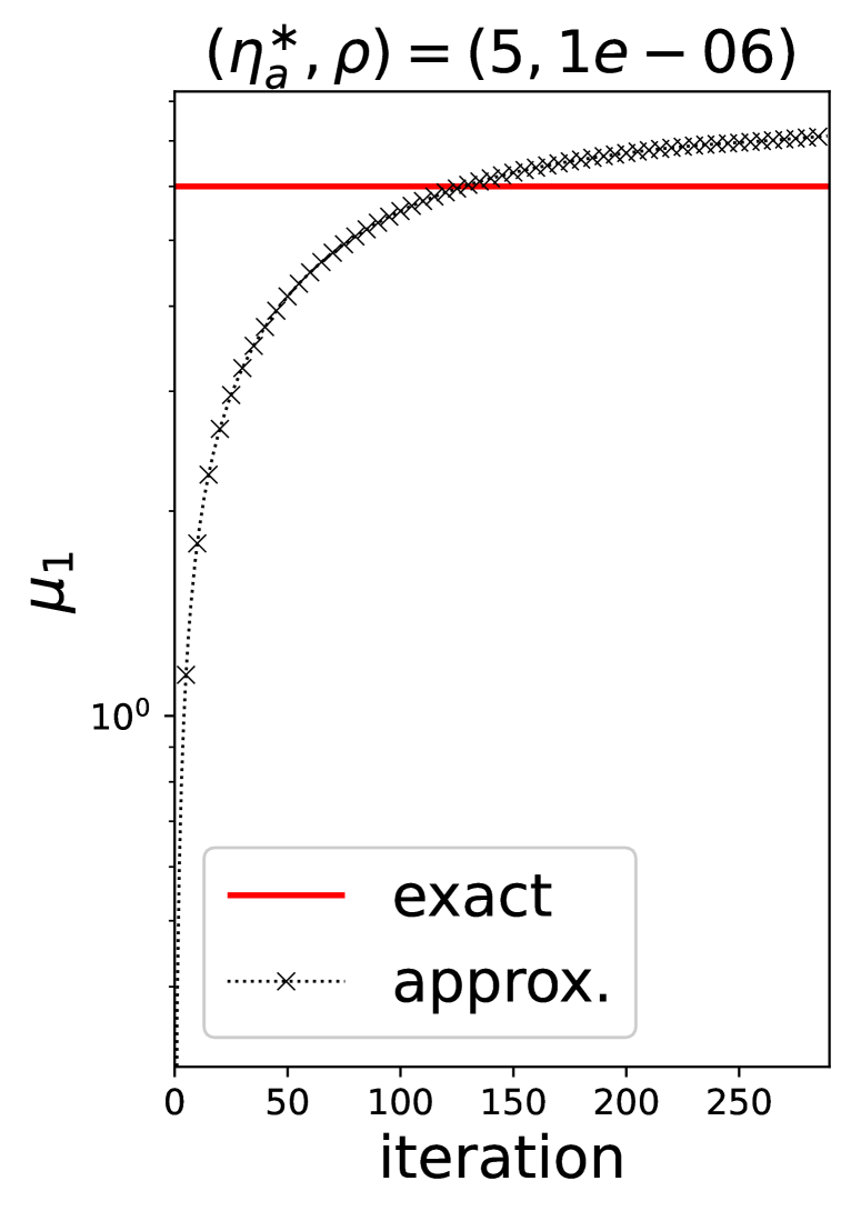
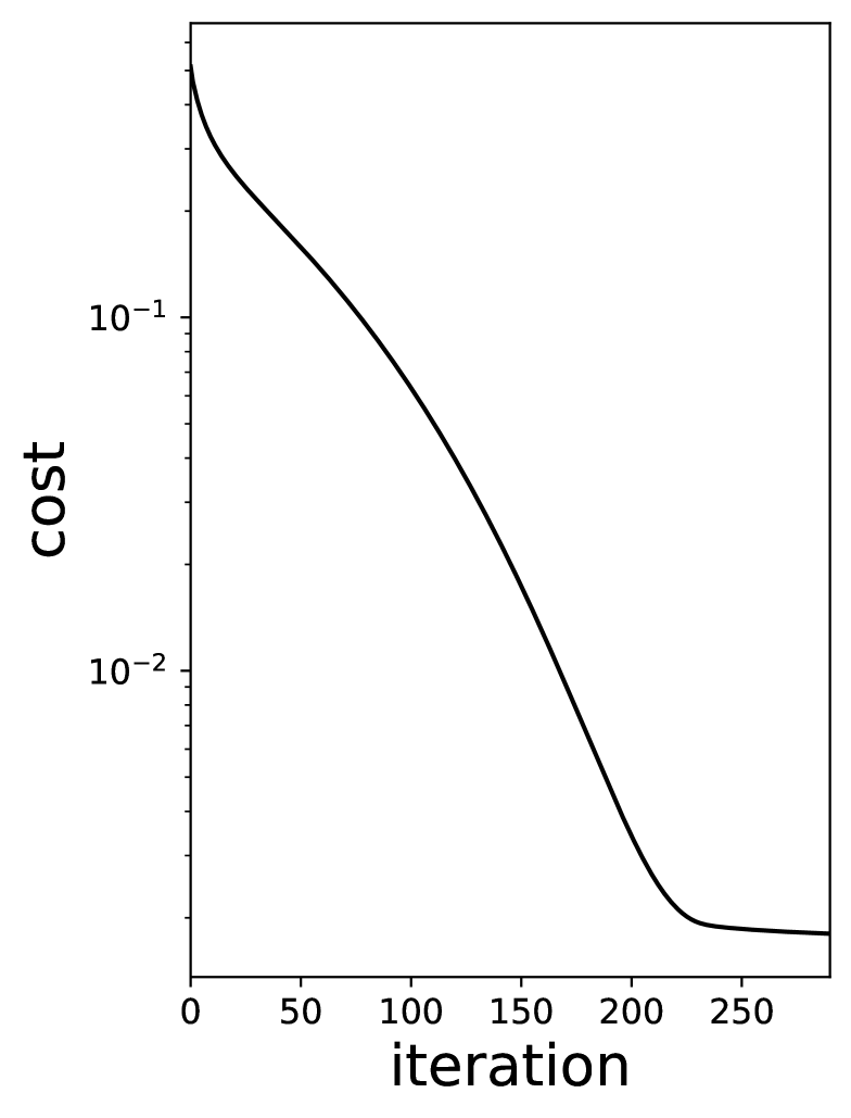
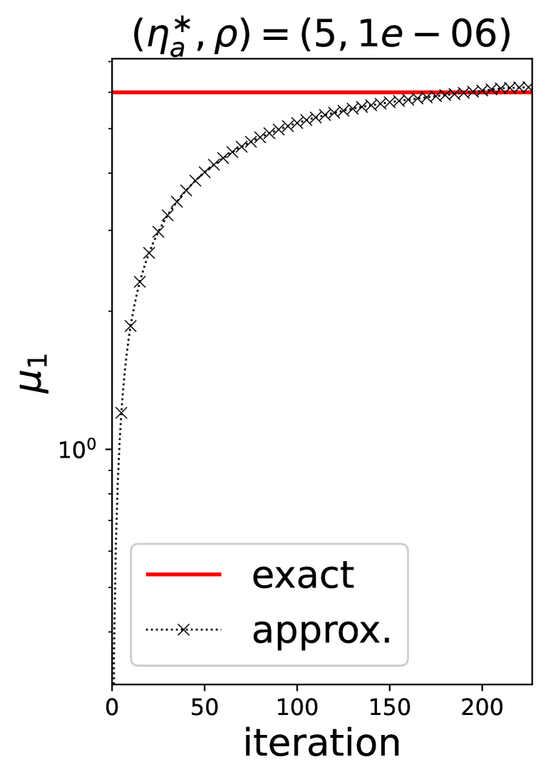
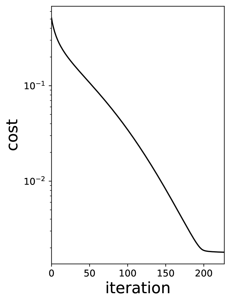
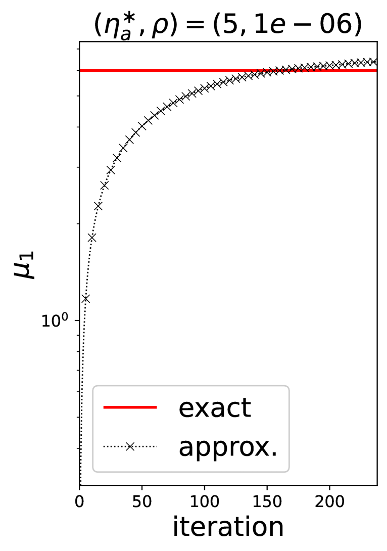
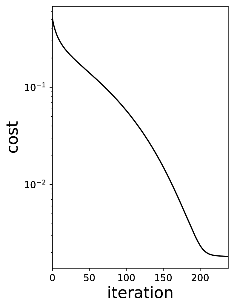
Figure 11. Effect of choice of initial guess

4.9. Numerical tests with point source and non-circular boundary interface

We conduct numerical experiments using a point source to reconstruct a non-circular boundary interface, based on the setup from subsection 4.8, with some modifications. Using $f(x)=100\delta(x)$ as the point source, we reconsider the reconstruction problem shown in Figure 6. The results, in Figure 12, compare scenarios with and without noise, with the regularization parameter $\rho$ set to $10^{-7}$. The problem becomes more ill-posed, as small perturbations in the measurements lead to significant discrepancies in the reconstruction. Apparently, reconstructing a non-circular boundary interface with a point source is particularly challenging.

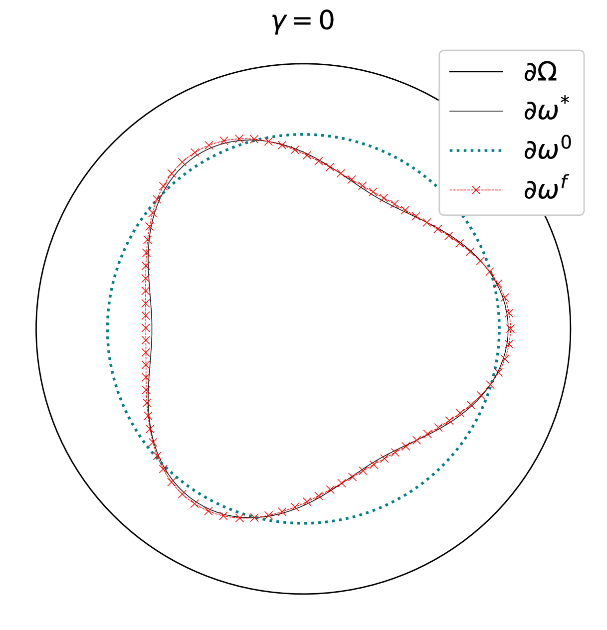
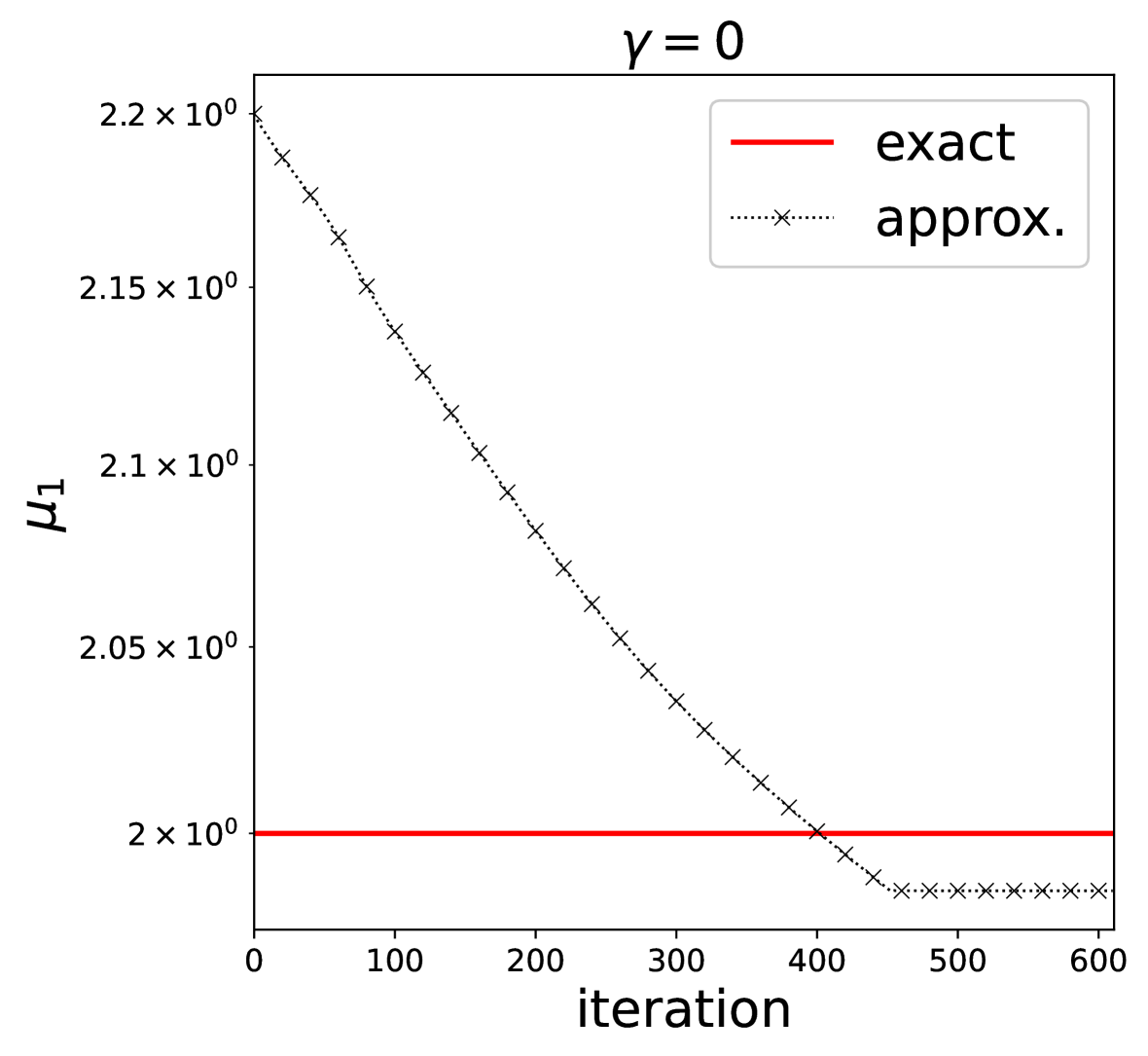
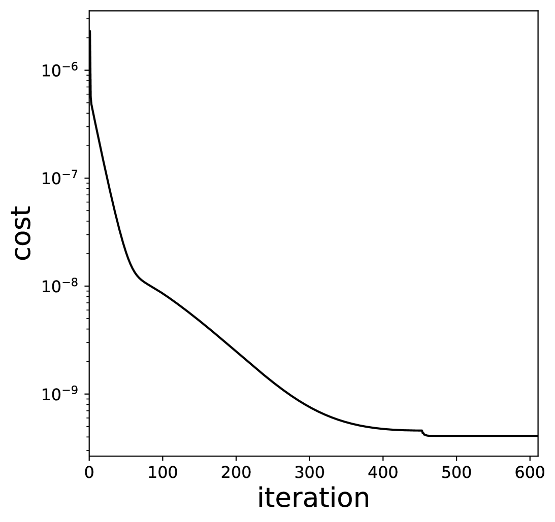
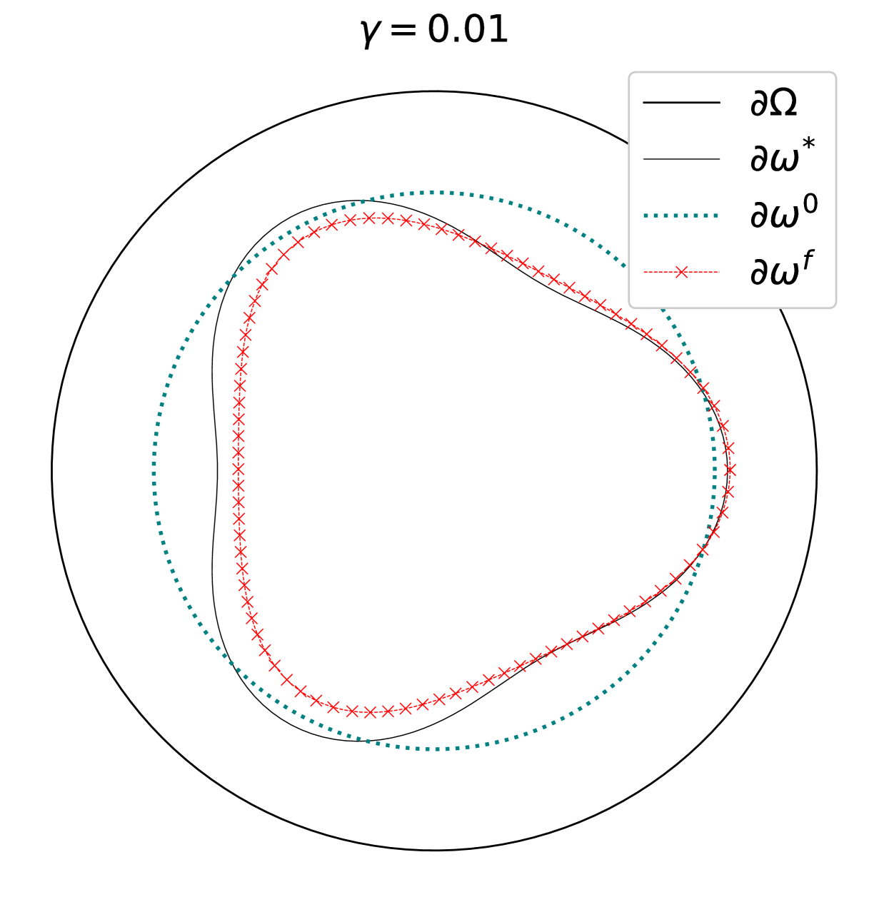
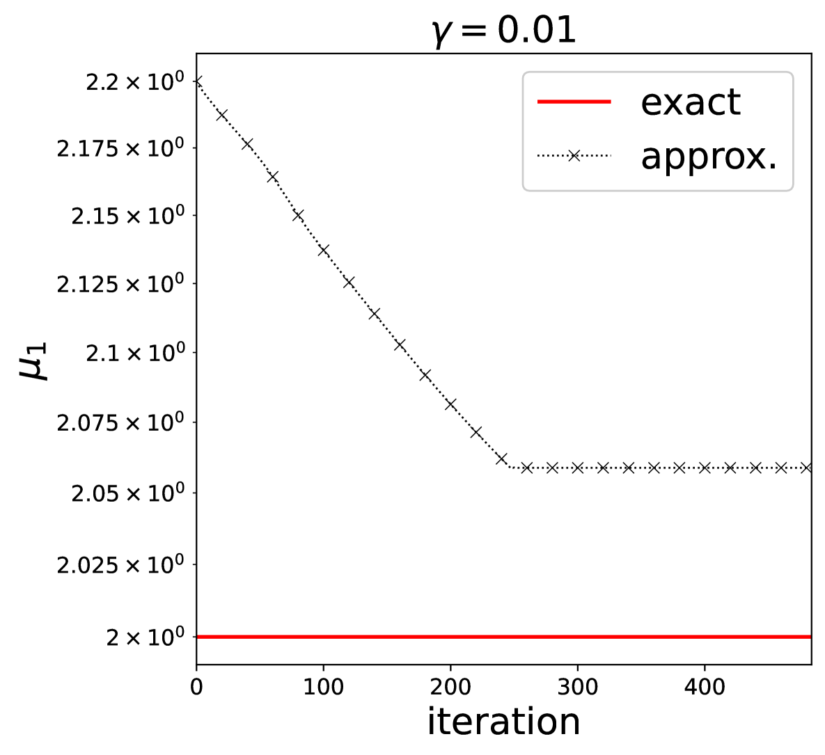
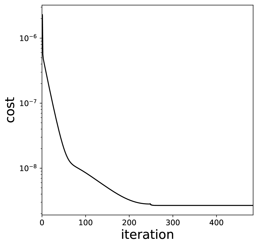
Figure 12. Results for a non-circular boundary interface with $f(x)=100\delta(x)$ under exact (first three columns from the left) and noisy measurements ($\gamma=0.01$)

We also test our approach with a more complex boundary interface, parameterized as:

$$\partial\omega^{\ast}=\left\{5(0.4+0.12\cos(3t))\begin{pmatrix}\cos{t}\\ \sin{t}\end{pmatrix},\forall t\in[0,2\pi)\right\}.$$

We set $f(x)=100\delta(x)$ and $\mu_{1}^{\ast}=6$. Reconstruction results using both exact measurements and noisy data with $\gamma=0.01$ are shown in Figure 13. Reconstruction is highly accurate with exact measurements, but introducing noise ($\gamma=0.01$) makes it slightly more challenging. However, the reconstructed boundary interface and coefficient $\mu$ remain satisfactory. For exact measurements, we set $\rho=5\times 10^{-6}$, and for noisy data, $\rho=5\times 10^{-5}$. These reconstructions, like the previous examples, depend heavily on the initial guess.

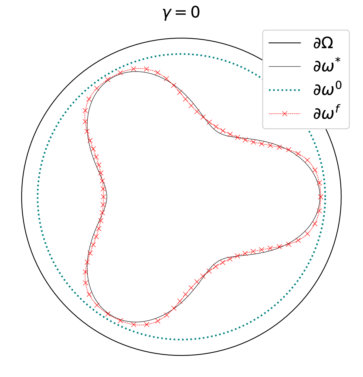
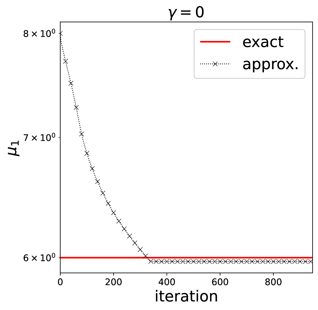
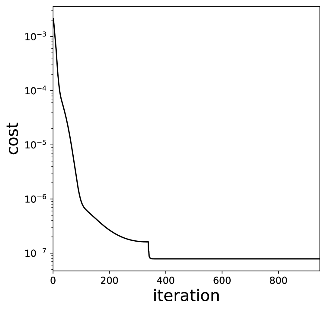
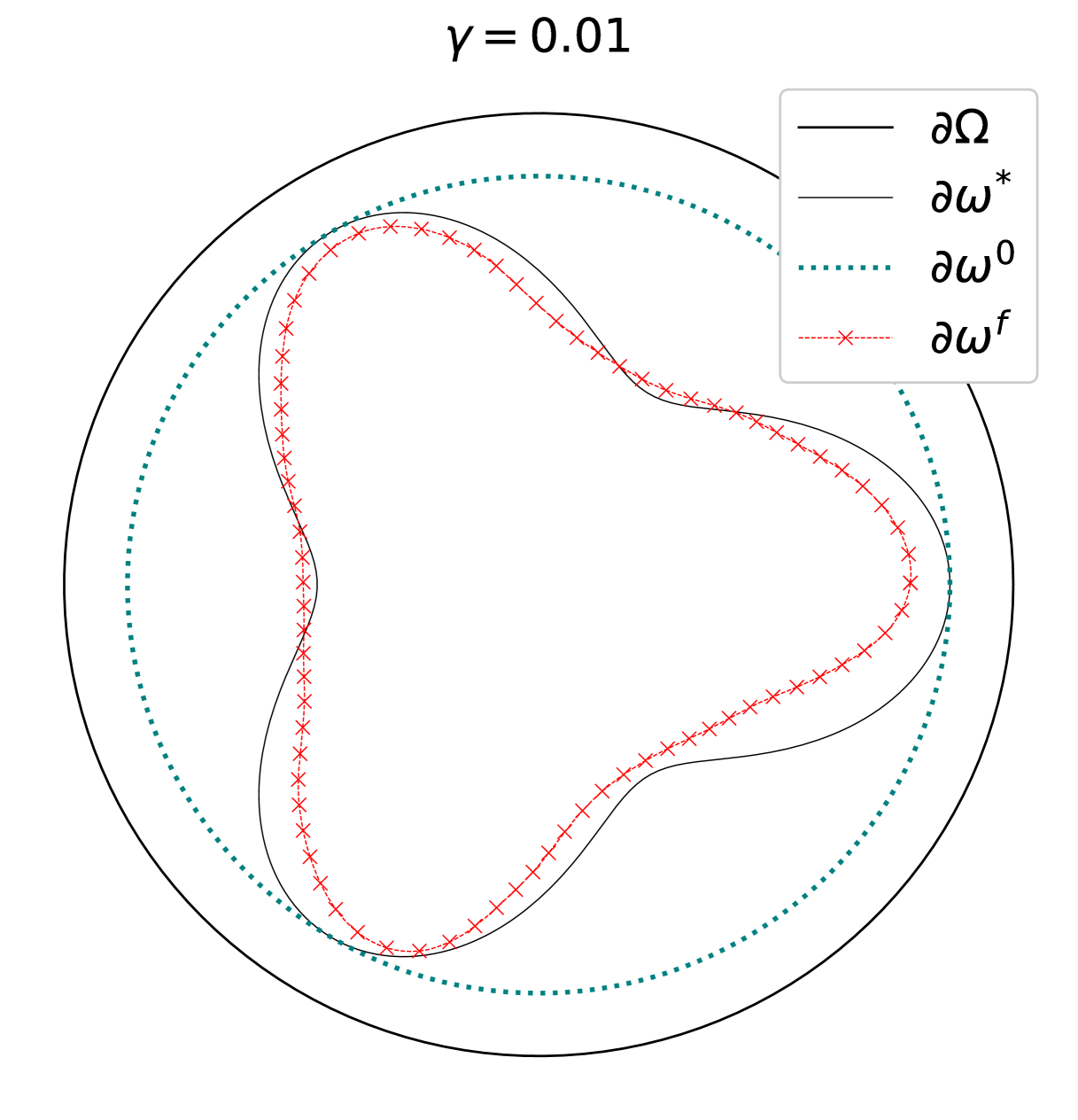
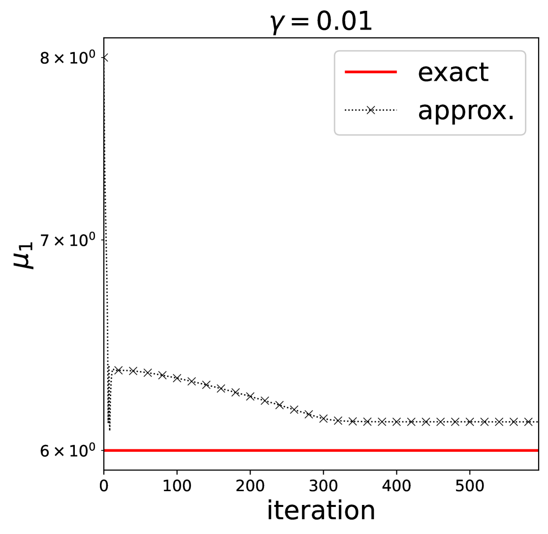
Figure 13. Results for a smooth non-circular boundary interface with $f(x)=100\delta(x)$ and $\mu_{1}^{\ast}=6$ under exact (first three columns from the left) and noisy measurements ($\gamma=0.01$)

Finally, we consider a smaller boundary interface in the last test of this subsection. This time, ${\color[rgb]{0,0,0}}^{\ast}$ is parametrized as:

$$\partial\omega^{\ast}=\left\{8(2+0.6\cos(4t))\begin{pmatrix}\cos{t}\\ \sin{t}\end{pmatrix},\forall t\in[0,2\pi)\right\}.$$

The computational setup remains the same, but instead of fixing $\rho$, we apply (36) to evaluate its impact and accuracy. The reconstruction results, shown in Figure 14, were obtained with $s=10$ for exact measurements and $s=1$ for noisy ones. As expected, reconstructing smaller boundary interfaces, especially those farther from the exterior boundary, is challenging. Reconstruction accuracy decreases with even small amounts of noise. However, the method successfully identified concavities in the boundary interface, with the reconstructed geometry closely approximating the exact shape and providing a reasonably accurate absorption coefficient. Figure 14 also includes plots of the histories of values for $\mu_{1}$, cost values, and $\rho$.

From this point forward, all reconstructions use the balancing principle (36). The source is fixed as $f(x)=100\delta(x)$, $\mu_{1}^{\ast}=6$ and noisy measurements mean the noise level is set to $\gamma=0.005$.

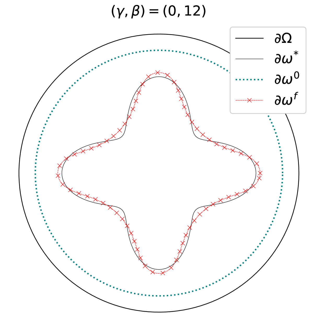
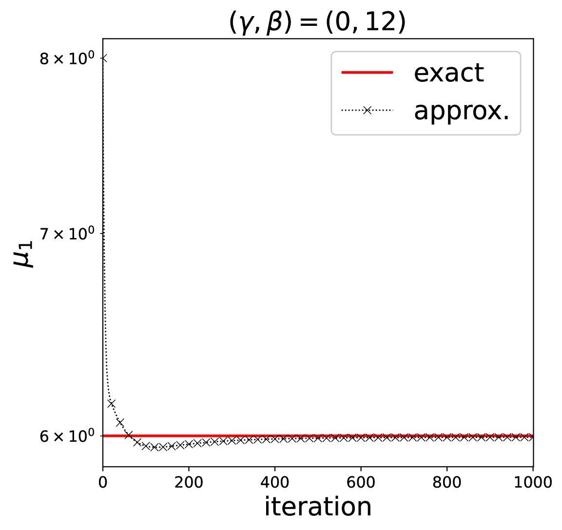
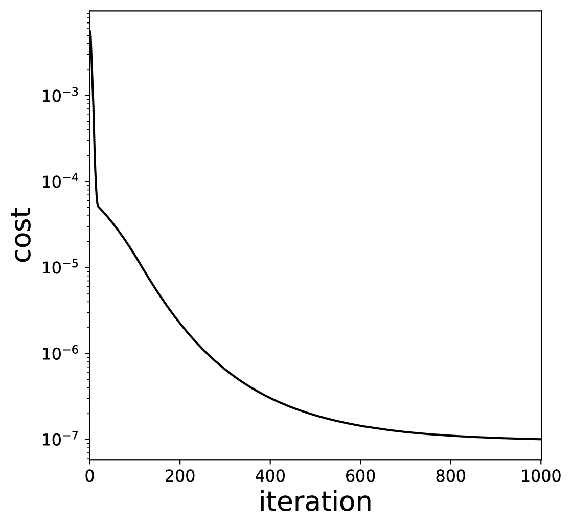
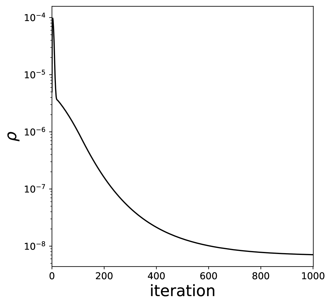
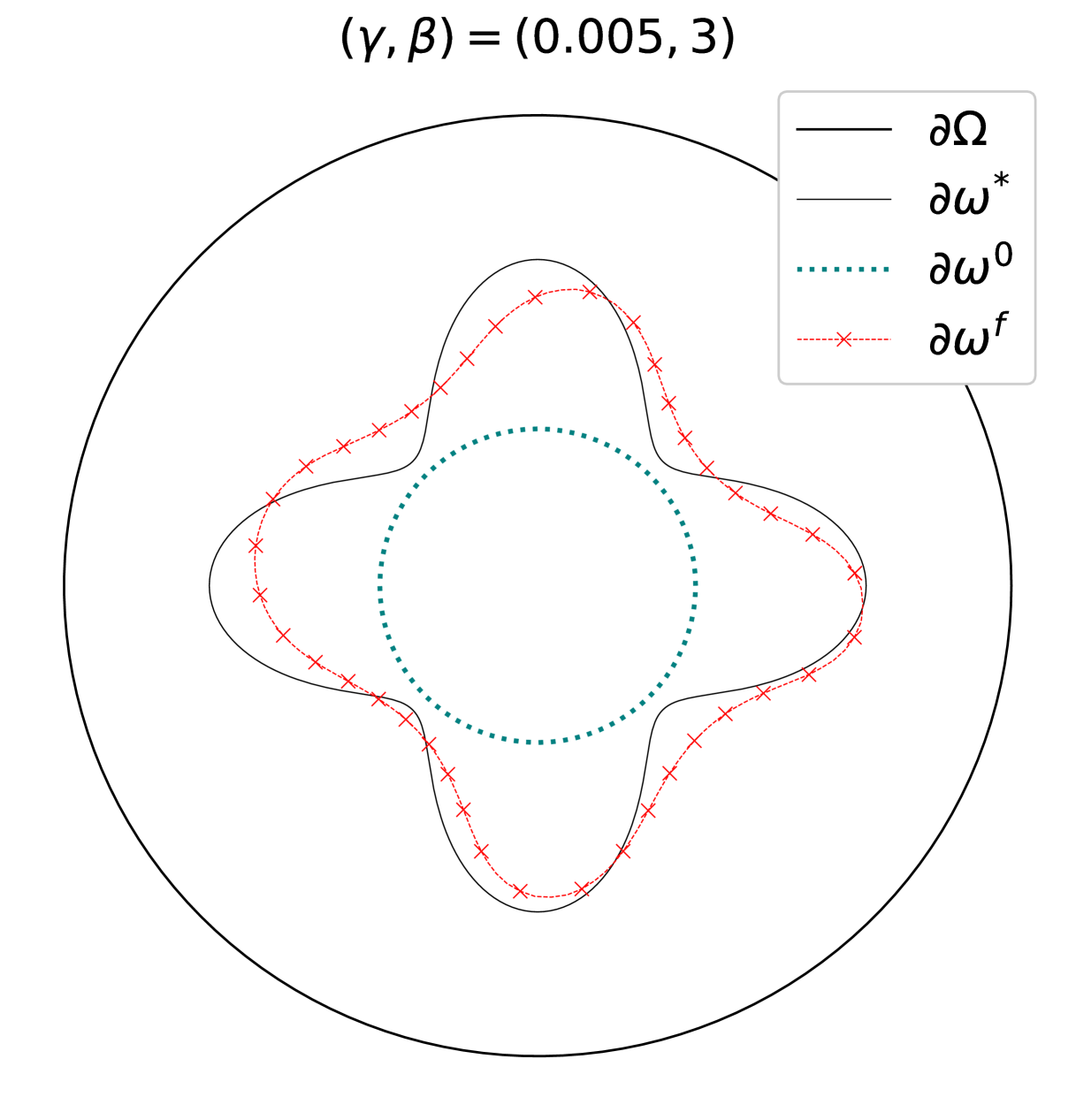
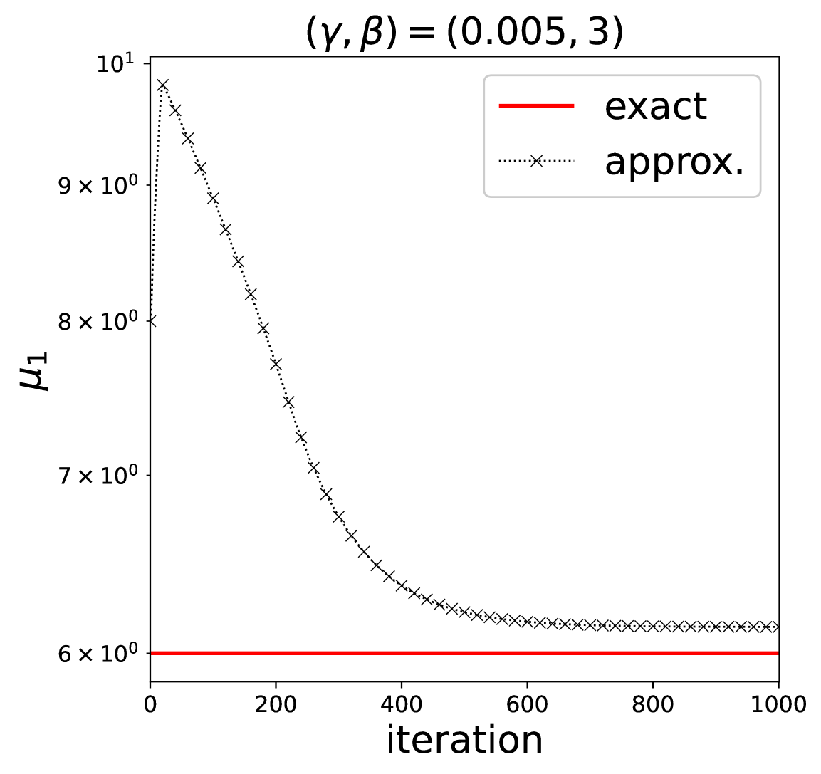
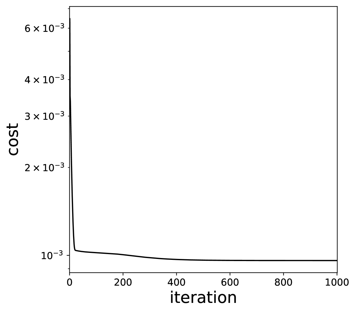
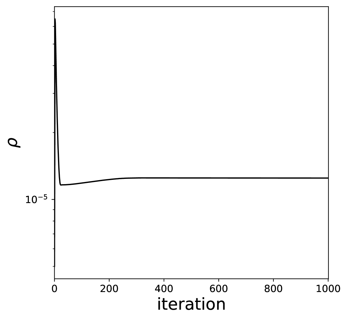
Figure 14. Results for a smooth non-circular boundary interface with $f(x)=100\delta(x)$ and $\mu_{1}^{\ast}=6$ under exact and noisy measurements ($\gamma=0.005$)

4.10. Numerical tests with point source and boundary interface with sharp edges

For the next experiment, we consider boundary interfaces with sharp edges, which violate our regularity assumption. However, we include these cases to test our numerical method. The setup remains the same as in the previous subsection, with the only change being the modified boundary interface geometry that needs reconstruction. Specifically, we test a square boundary interface and an inverted T-shaped polygon.

The reconstruction results are shown in Figures 15 and 16 for exact and noisy measurements. In Figure 15, reconstructing the square’s vertices is challenging. Even so, the method successfully detects the edges with good accuracy. Noise significantly affects the reconstruction, making it hard to accurately deduce the boundary geometry, but the method still identifies the interface and nearly reconstructs $\mu_{1}^{\ast}$ accurately.

A similar observation is made for the inverted T-shaped polygon in Figure 16, which is more challenging. Although the vertices and edges are not reconstructed, the method accurately determines $\mu_{1}^{\ast}$, even with noise, and identifies concavities within the boundary interface. These examples demonstrate the method’s effectiveness in reconstructing non-smooth boundary interfaces.

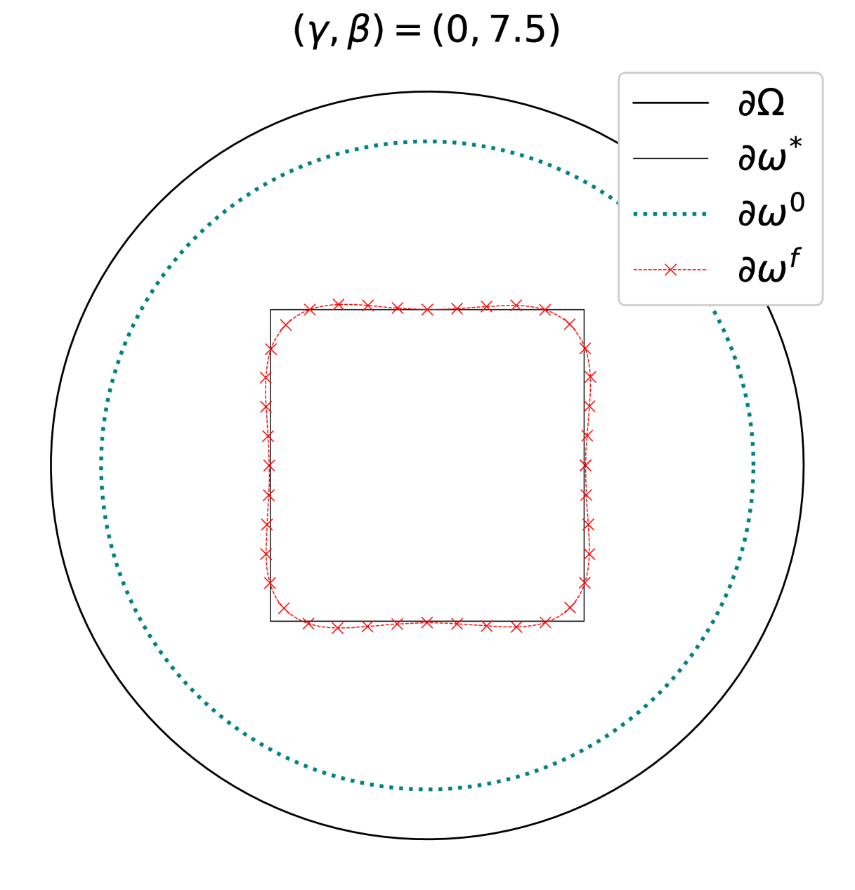
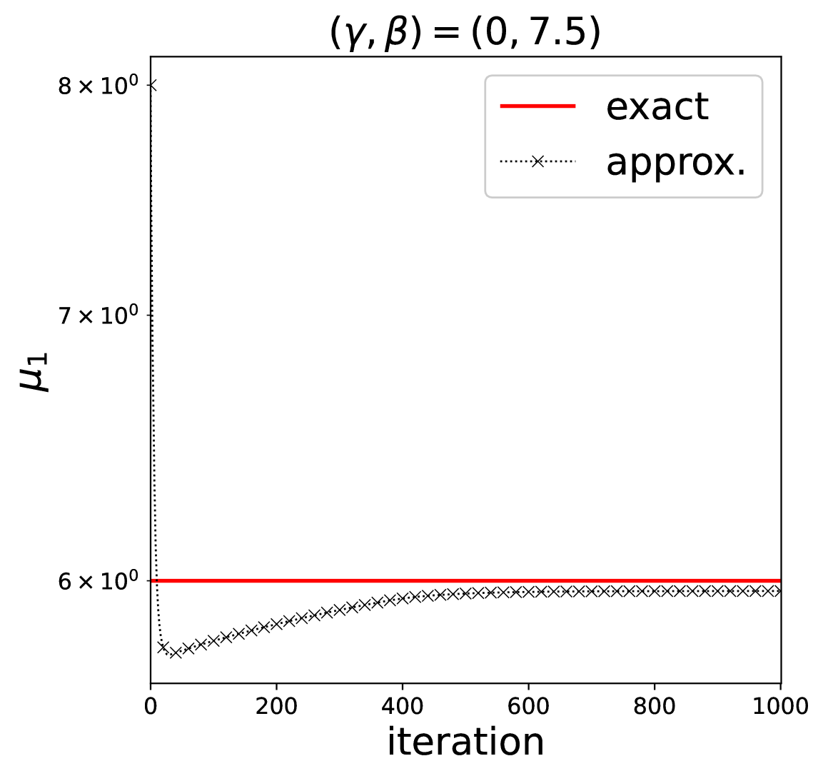
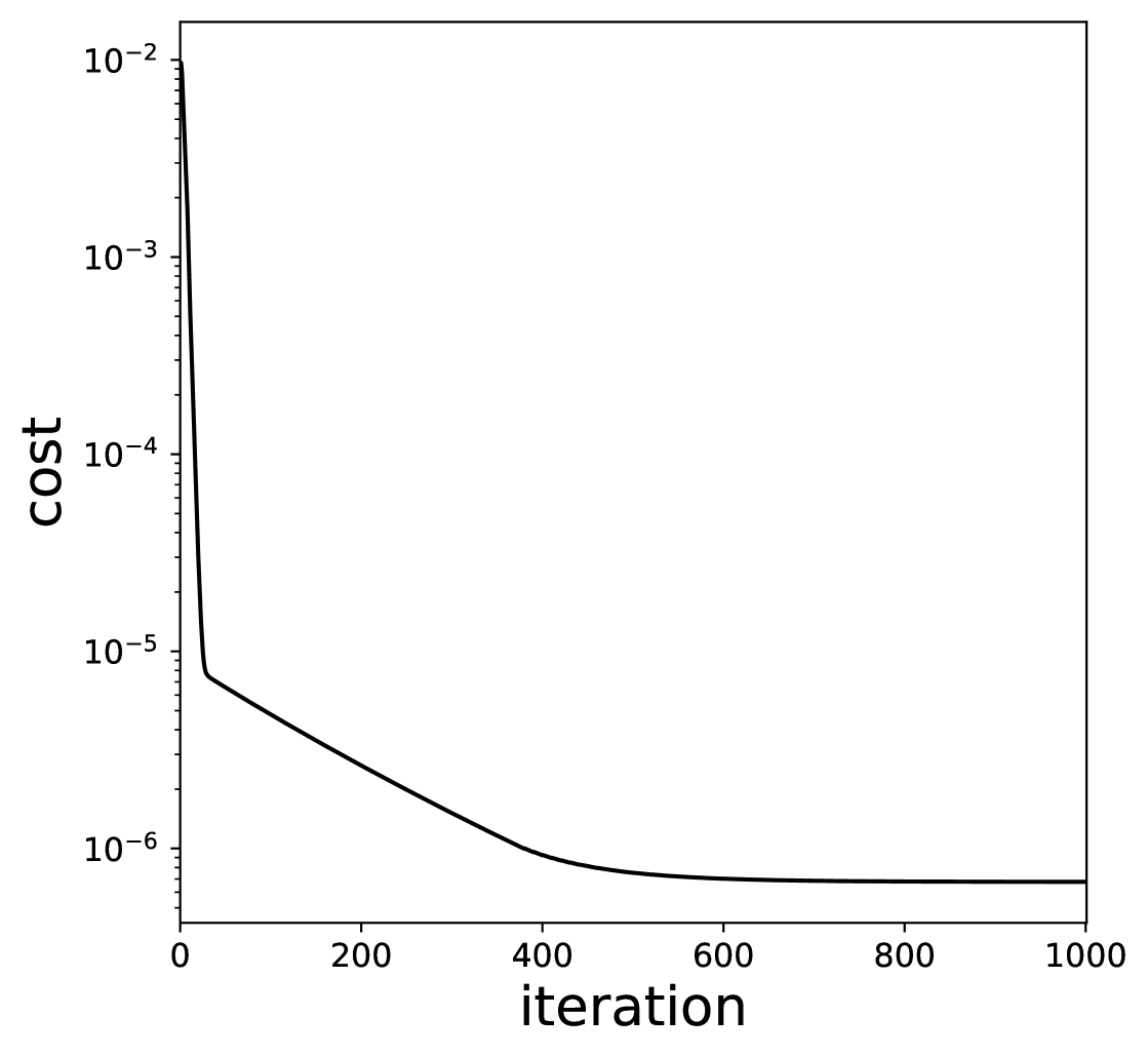
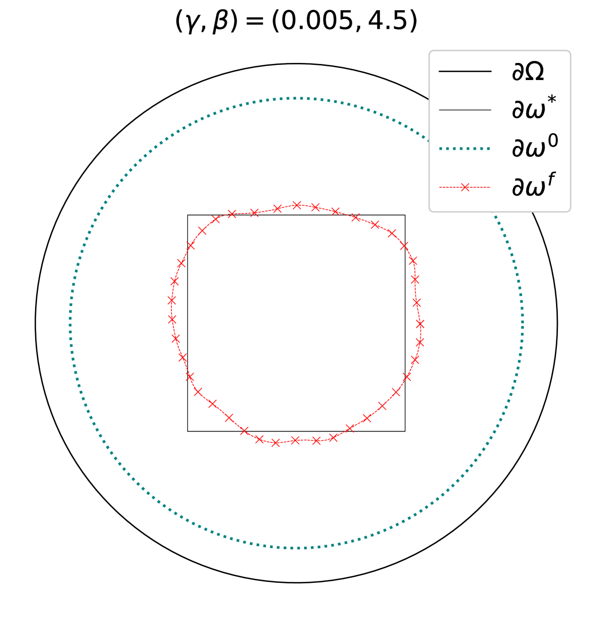
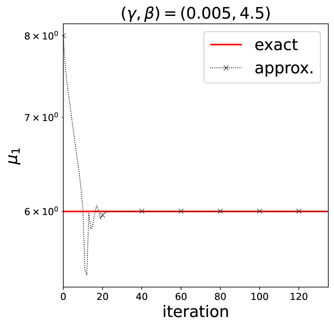
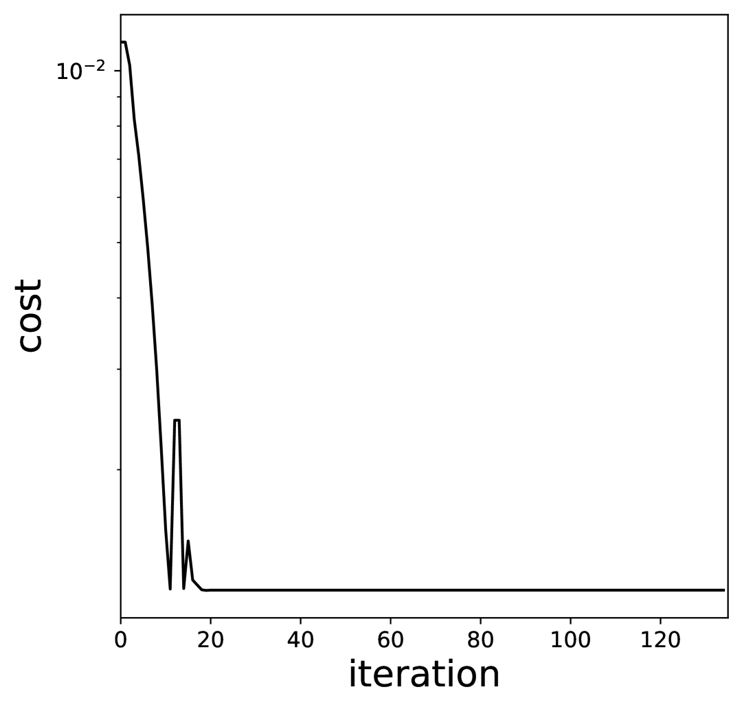
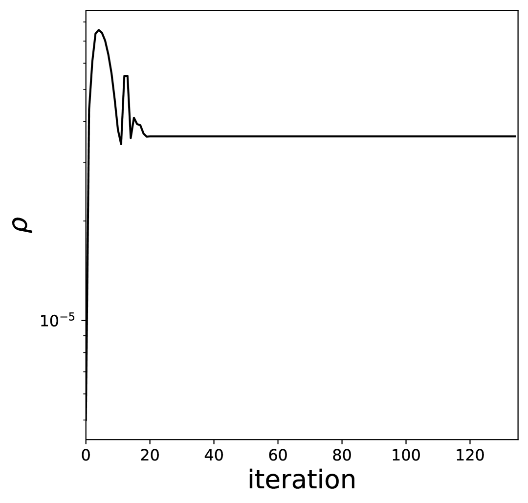
Figure 15. Results for a square boundary interface

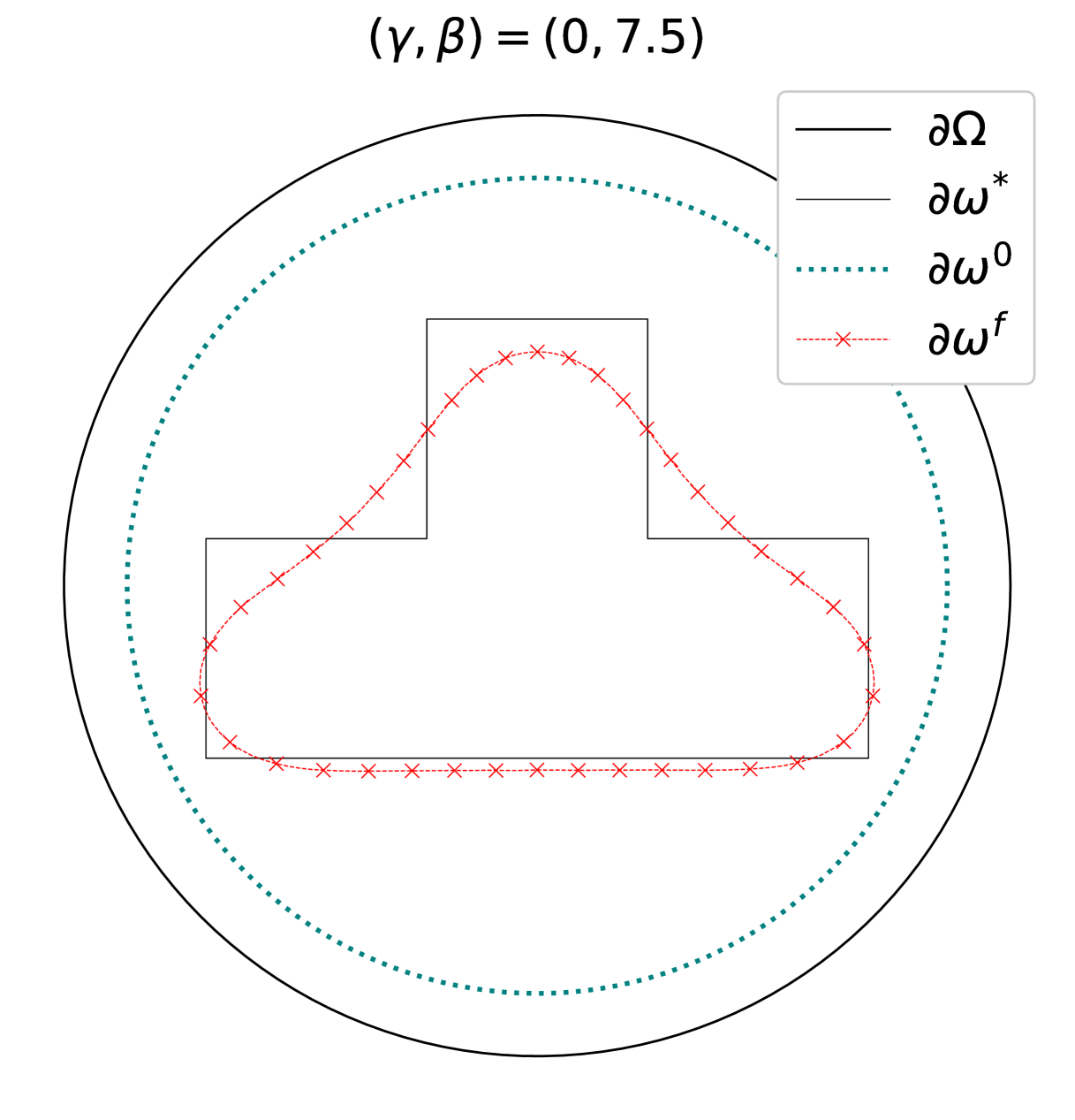
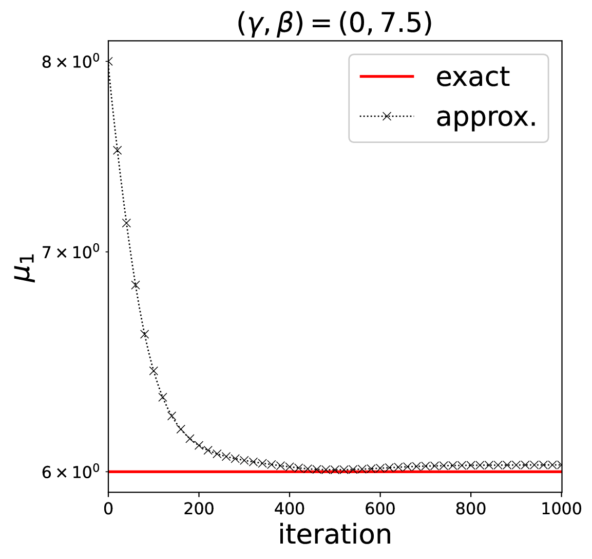
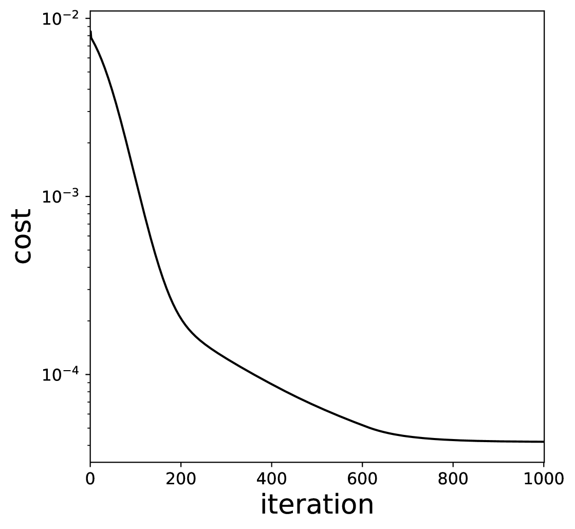
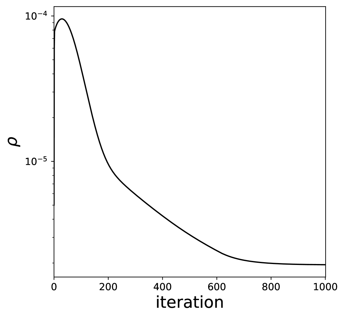
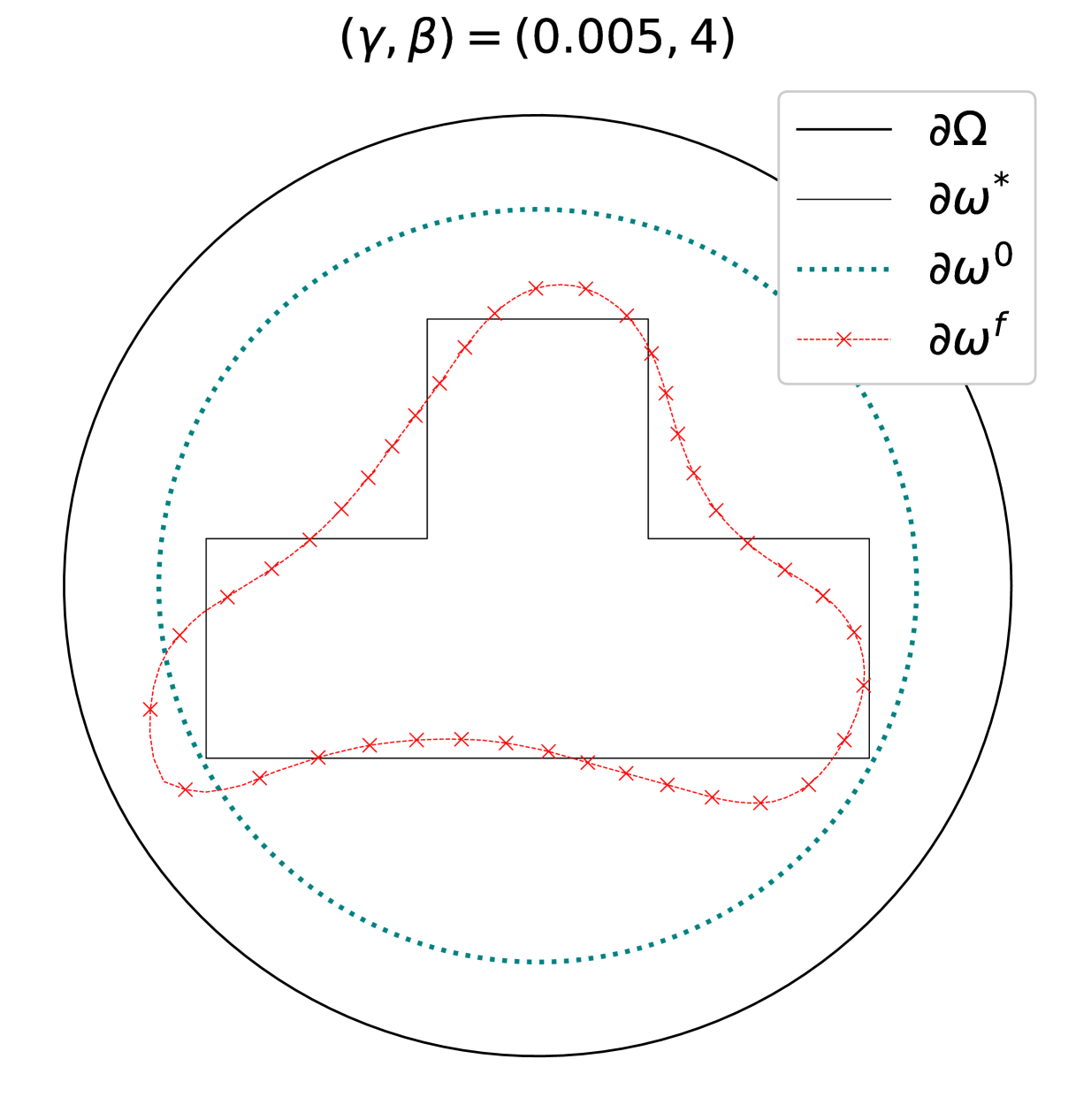
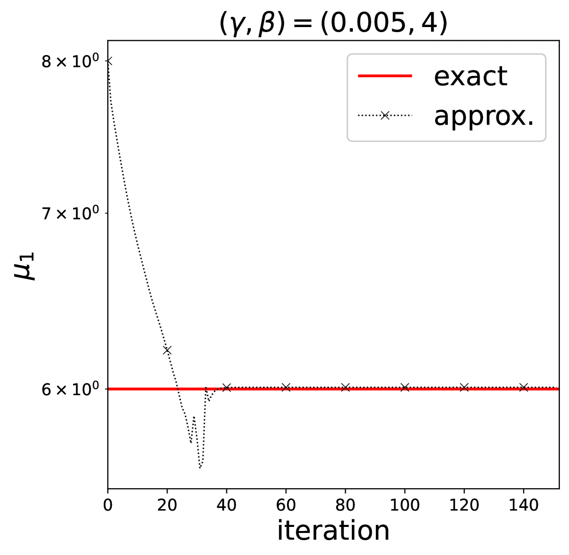
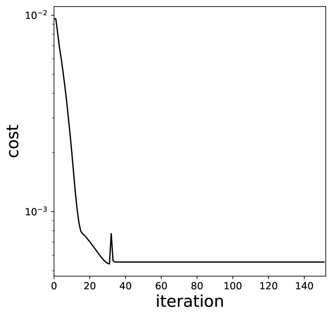
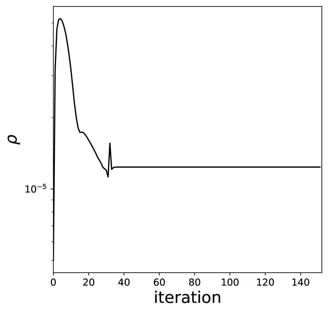
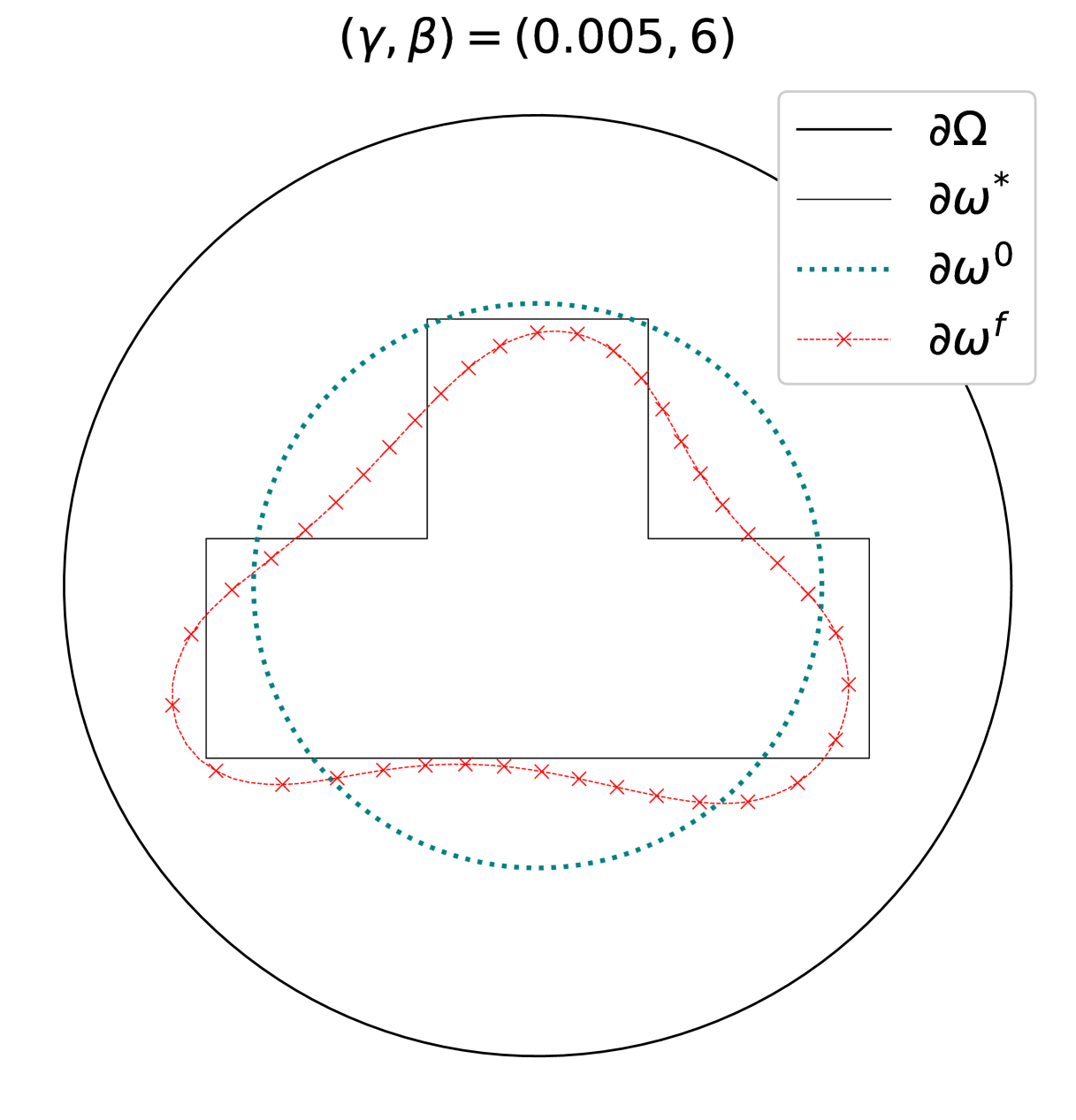
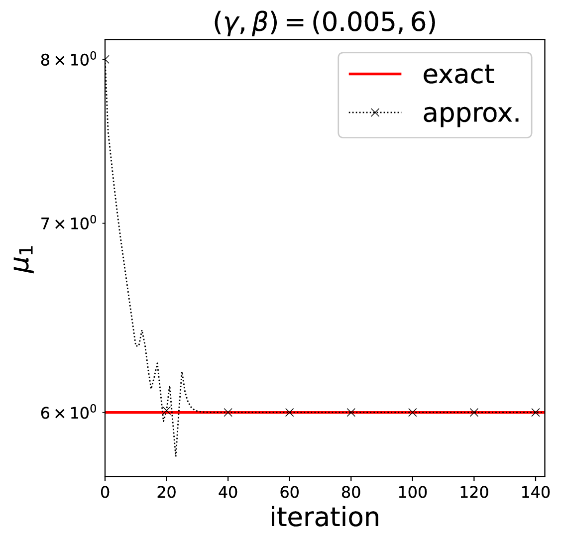
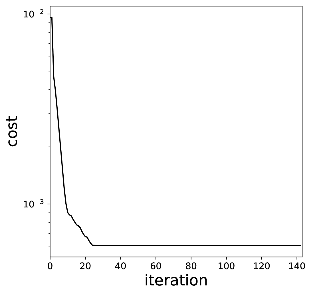
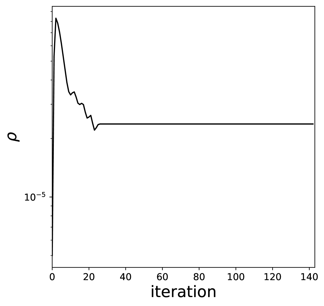
Figure 16. Results for an inverted T-shaped boundary interface

4.11. Numerical tests with sources close to the boundary

To conclude our numerical examples, we consider cases with multiple (point) sources. The sources are positioned near the boundary and we define $f$ as follows:

(39) $$f(x)=\sum_{i=1}^{M}\exp\left(1-\frac{(x-x_{i})^{2}+(y-y_{i})^{2}}{\epsilon^{2}}\right),$$

where $\epsilon>0$, $M\in\mathbb{N}$, and $(x_{i},y_{i})=(\bar{R}_{f}\cos{\theta_{i}},\bar{R}_{f}\sin{\theta_{i}})$ with $\theta_{i}\in[0,2\pi]$ and $\bar{R}_{f}\in(0,R)$. We set $\bar{R}_{f}=2.99$, and in this subsection, noisy measurements mean $\gamma=0.1$.

Figure 17 presents results for a circular boundary interface with parameters $(\mu_{0}^{\ast},\mu_{1}^{\ast})=(1,1.2)$ under exact and noisy measurements. Thick black dots indicate the source positions, which remain consistent across all cases, and reconstructions are achieved without perimeter regularization. Reconstruction accuracy decreases with fewer sources, as expected. For instance, when $\theta_{i}=(2\pi/3)i$ for $i=1,2,3$ (first column in Figure 17), the reconstructed shape deviates more from a circle compared to cases with more sources. Nonetheless, the results remain reasonable, even with noise. For these cases, we set $\epsilon=0.5$ in (39).

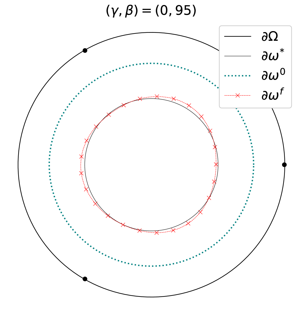
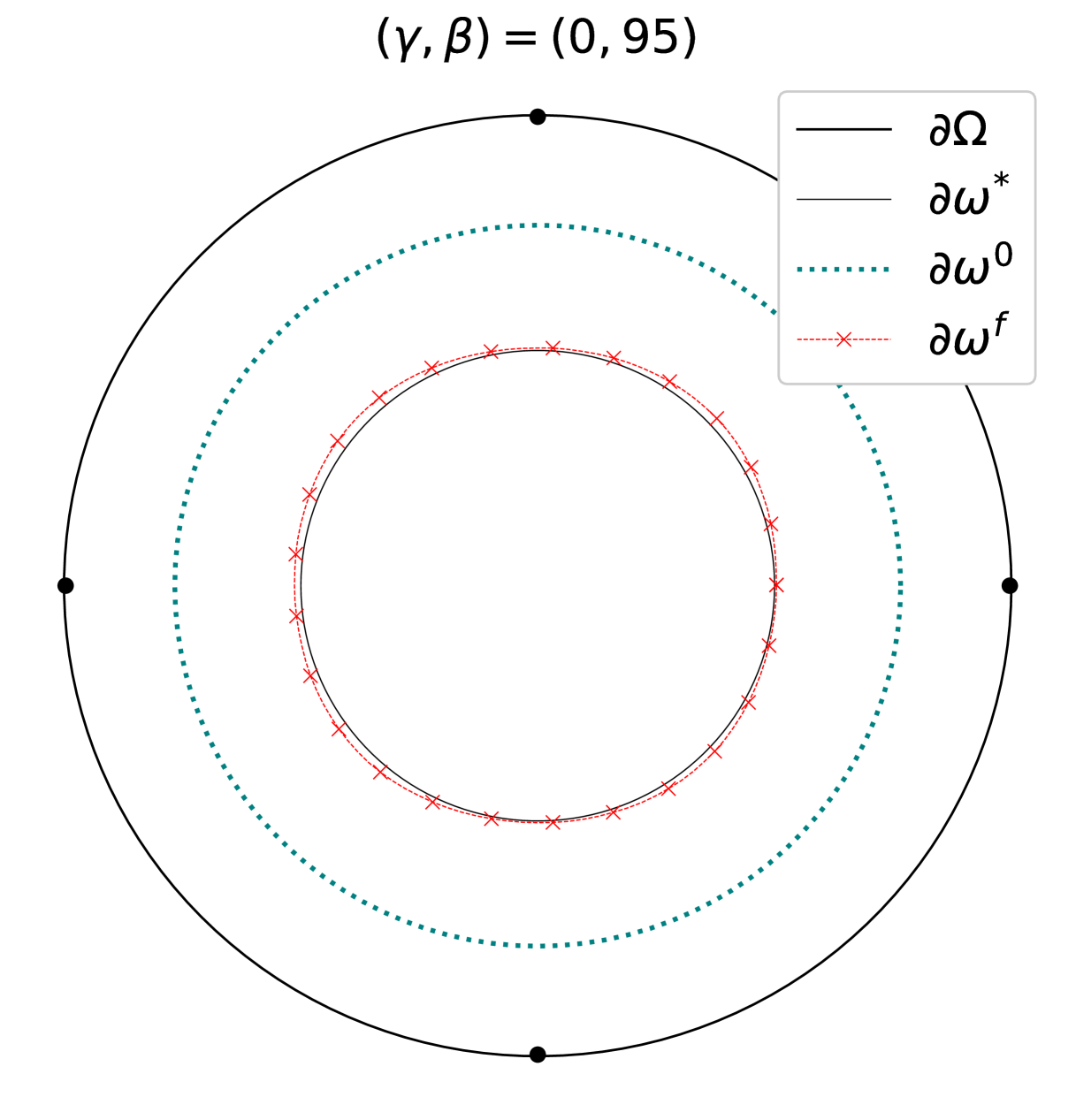
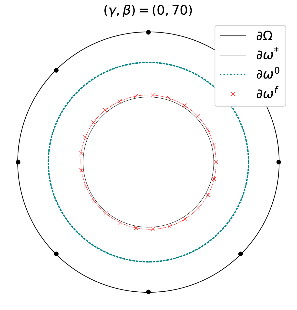
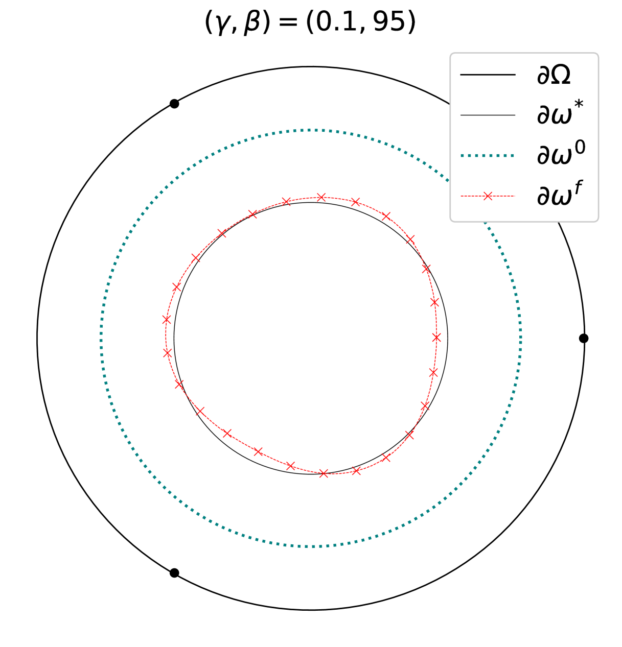
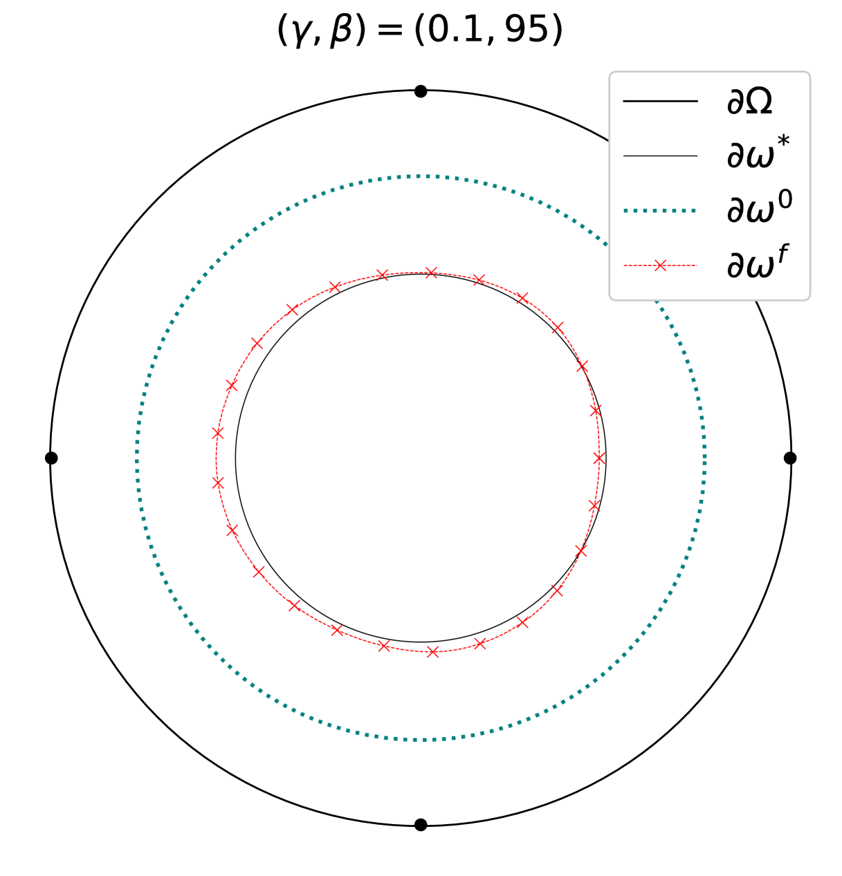
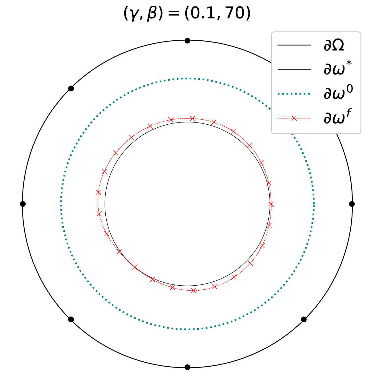
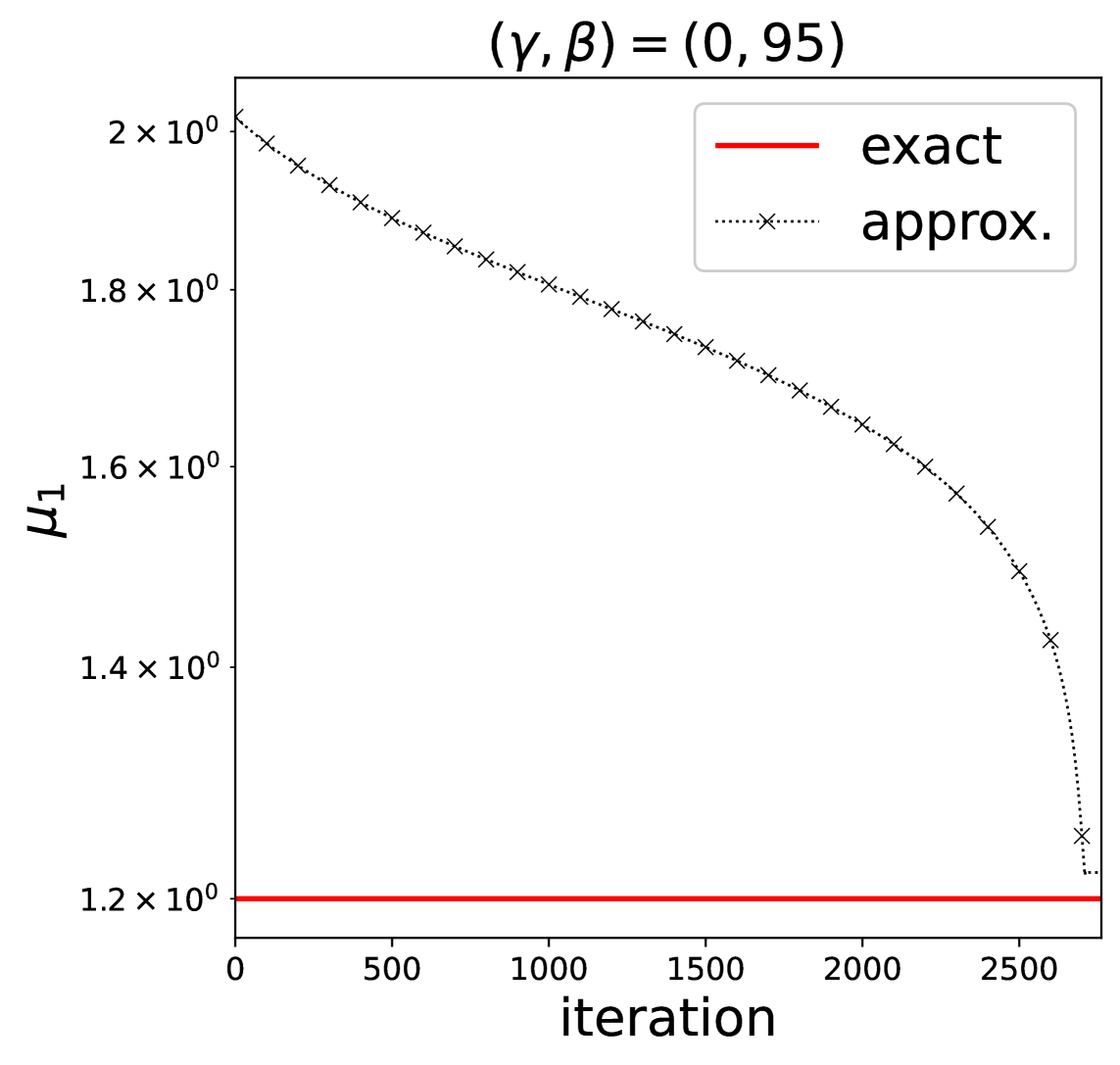
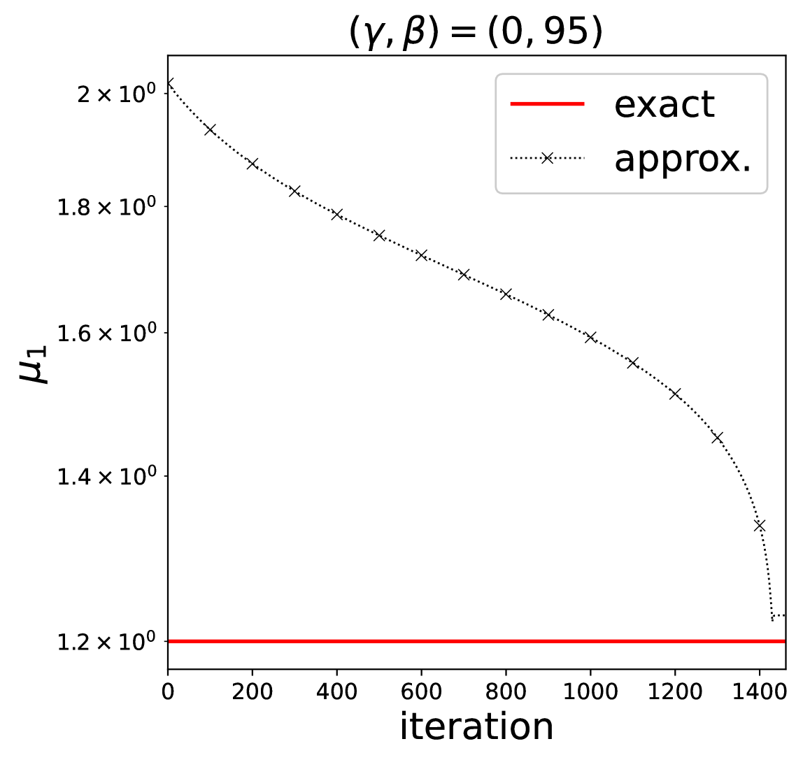
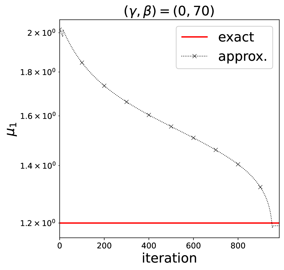
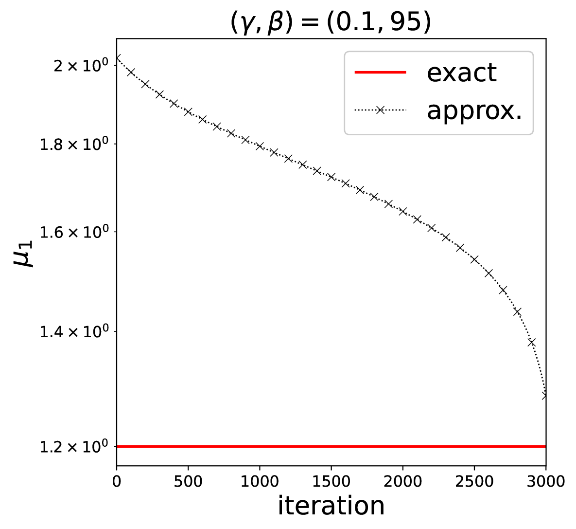
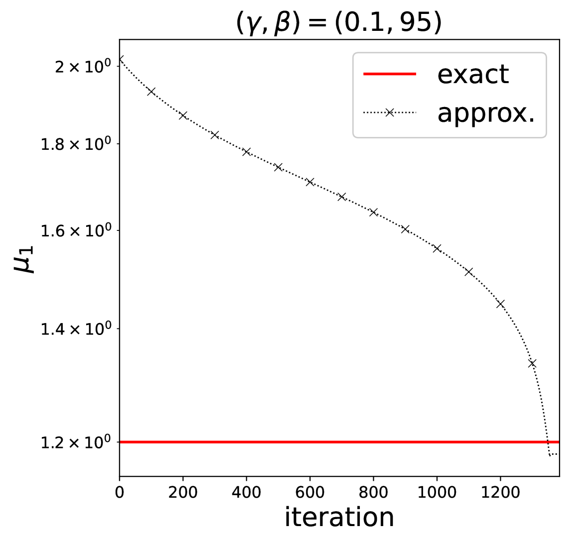
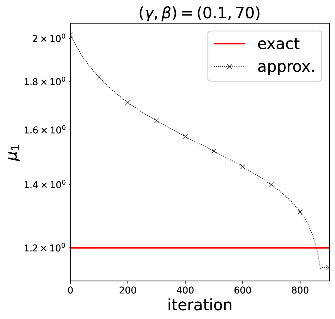
Figure 17. Results for a circular boundary interface with $f$ (given by (39) with $\epsilon=0.5$) of various positions and instances near the boundary and parameters $(\mu_{0}^{\ast},\mu_{1}^{\ast})=(1,1.2)$, under exact (first three columns from the left) and noisy measurements. No perimeter regularization was applied in any of the cases.

Next, we revisit the problem with eight sources positioned at $\theta_{i}=\frac{\pi}{4}i$, where $i=1,\ldots,8$ and examine the effect of varying $\epsilon$ in (39). We consider $\epsilon=0.5,0.3,0.2$ and apply perimeter penalization with a small weight. For the remaining experiments, we set $(\mu_{0}^{\ast},\mu_{1}^{\ast})=(1,6)$ and $\gamma=0.1$, using a peanut-shaped boundary interface.

Figures 18 to 20 show the results. Smaller $\epsilon$ values lead to less accurate reconstructions, making it harder to capture concave boundary regions. These results confirm that $\epsilon$ reflects the diffusion level of the sources.

Finally, we examine source positioning under noisy measurements. Using eight sources ($M=8$) with $\epsilon=0.5$ in (39), we fix the penalization parameter $\rho_{1}$ to $6\times 10^{-6}$. Reconstructions are evaluated for six configurations of source positions (see Figure 21 for two illustrations):

$$\text{Setup $k$}:\qquad\theta_{i}=\frac{k\pi}{3}+\frac{i\pi}{8},\qquad i=1,\ldots,8,\quad k=1,\ldots,6.$$

The reconstruction results are summarized in Figure 22. Even with noisy data, the method reconstructs the boundary interface and the unknown coefficient $\mu$ effectively. Also, observe that source positioning strongly influences accuracy, particularly for concave boundary regions. Reconstructions are less accurate in areas farther from the sources, as expected. Overall, the proposed method is robust and highly effective in reconstructing boundary interfaces with complex geometries under noisy measurements.

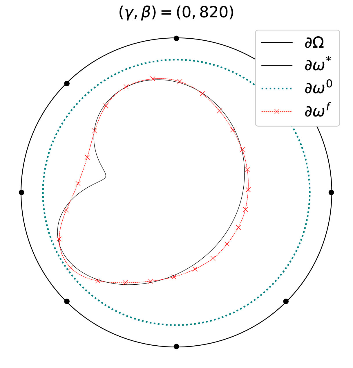
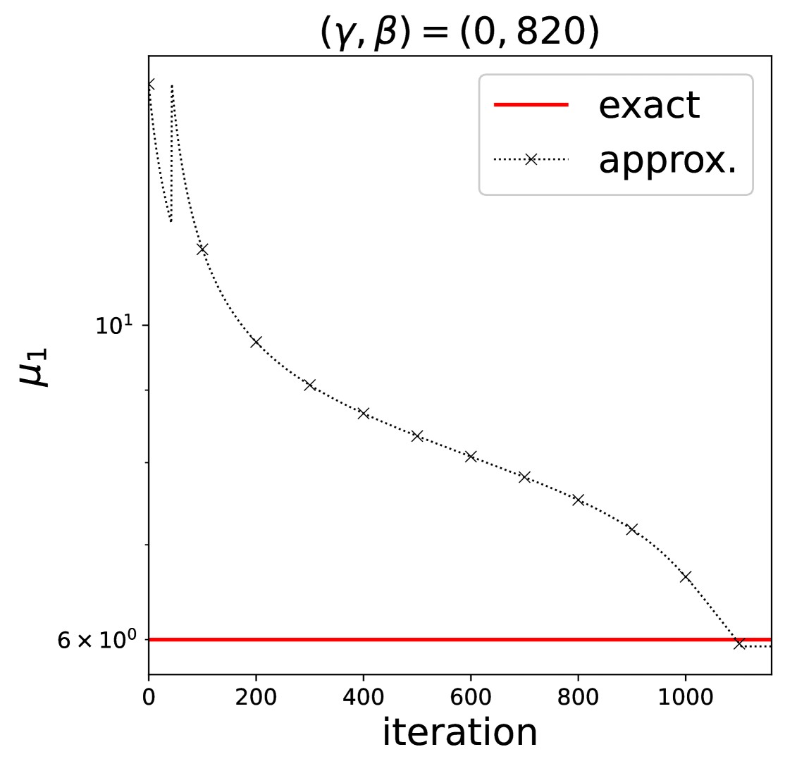
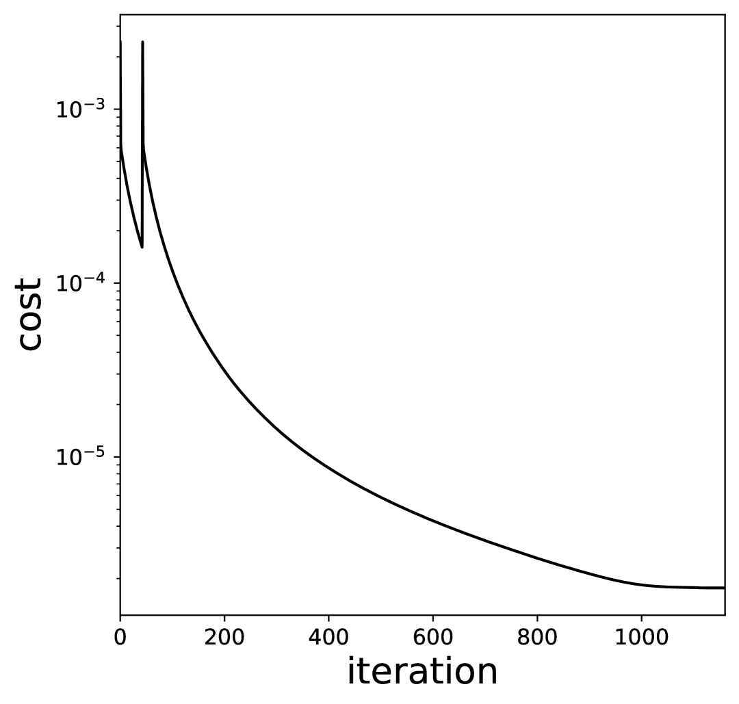
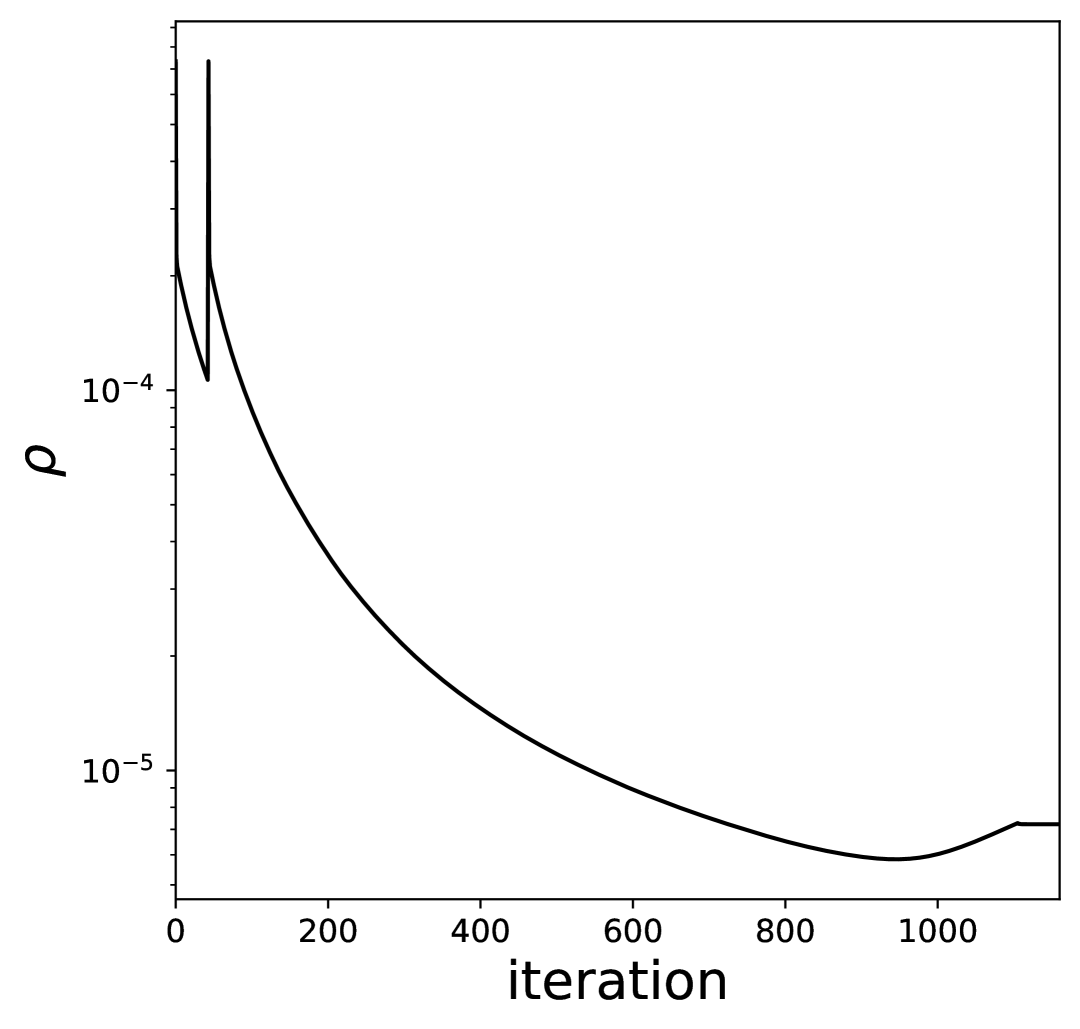
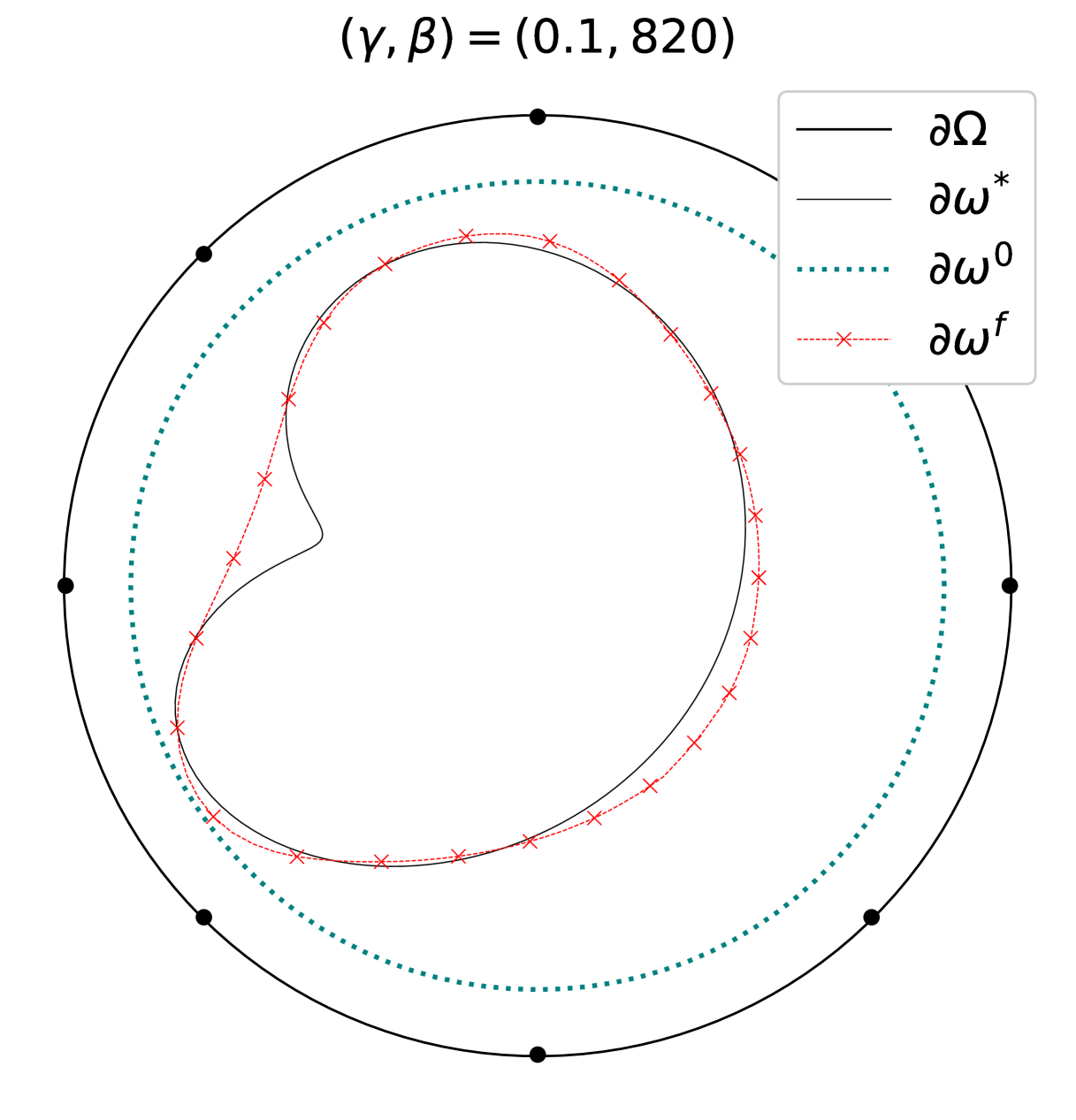
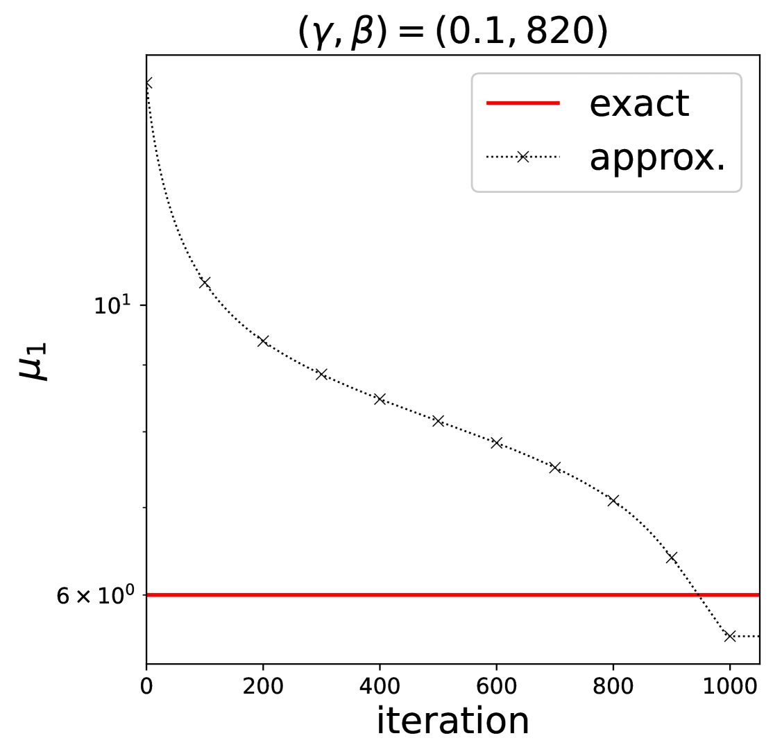
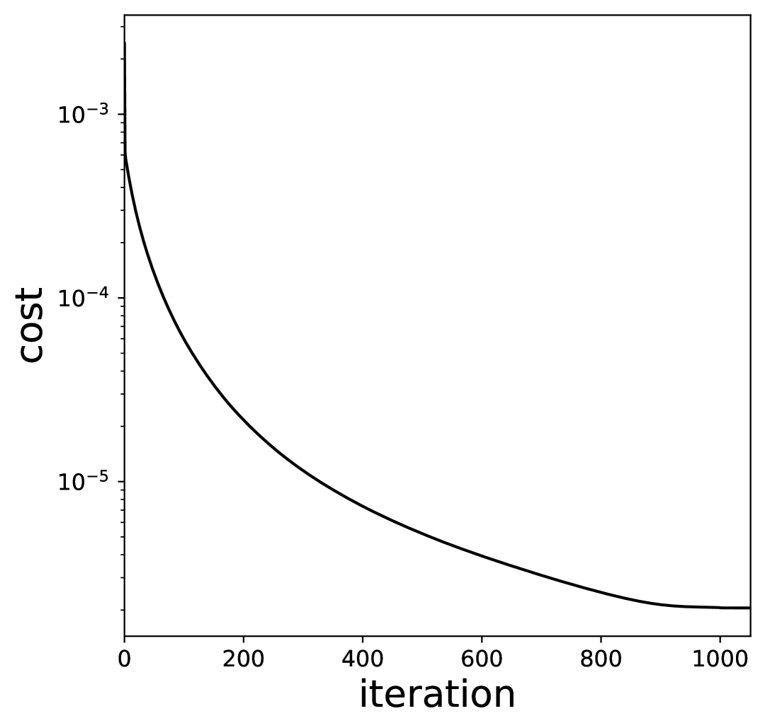
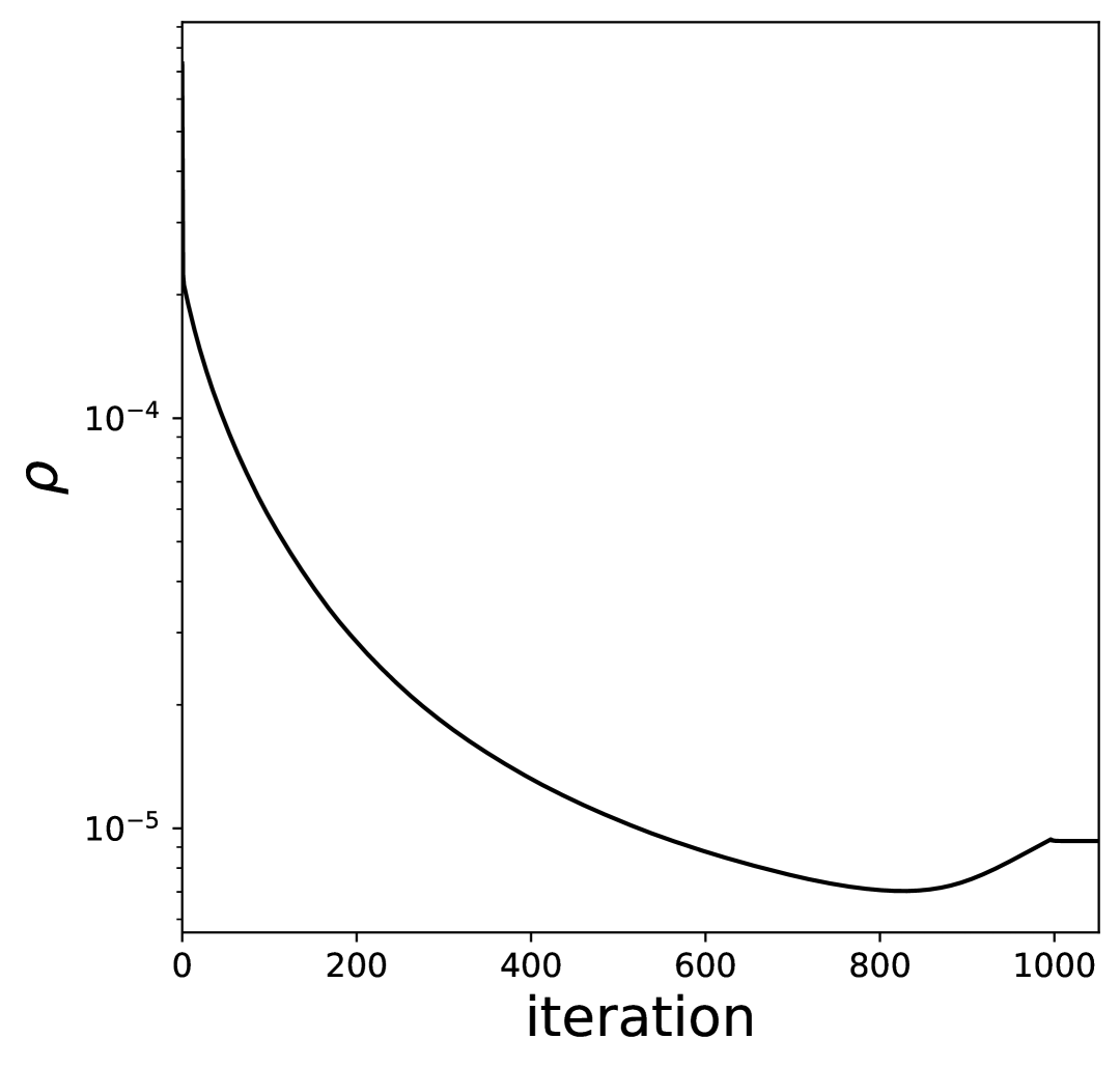
Figure 18. Results for a peanut-shape boundary interface with source $f$ (given by (39) with $\epsilon=0.5$) near the boundary, under exact (top row) and noisy measurements. Perimeter penalization was applied in all of the cases with $\rho_{1}=0.00004$.

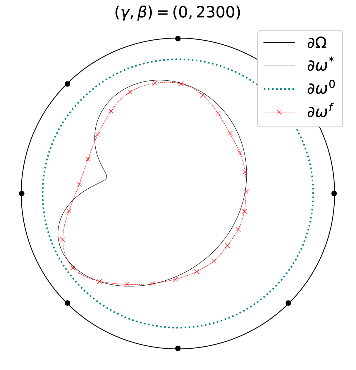
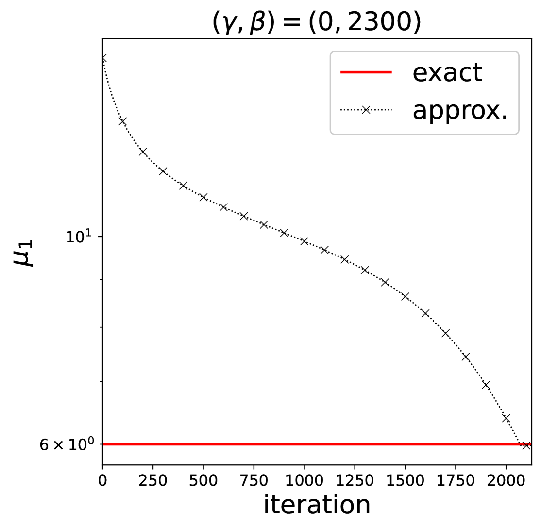
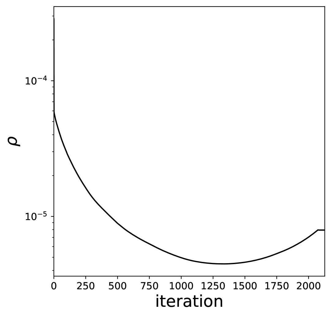
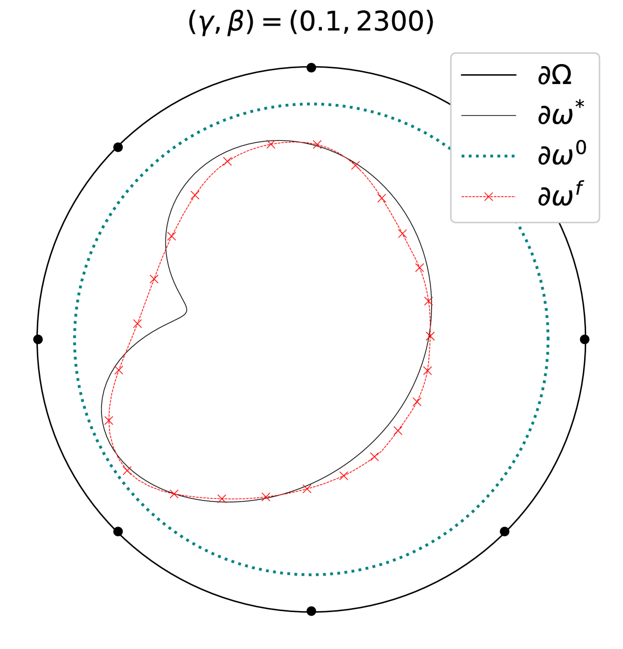
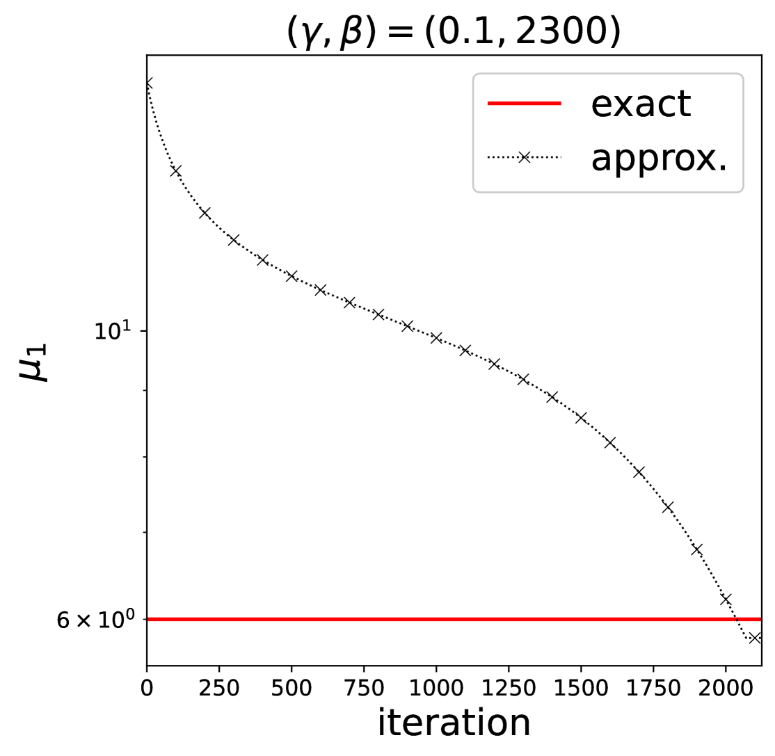
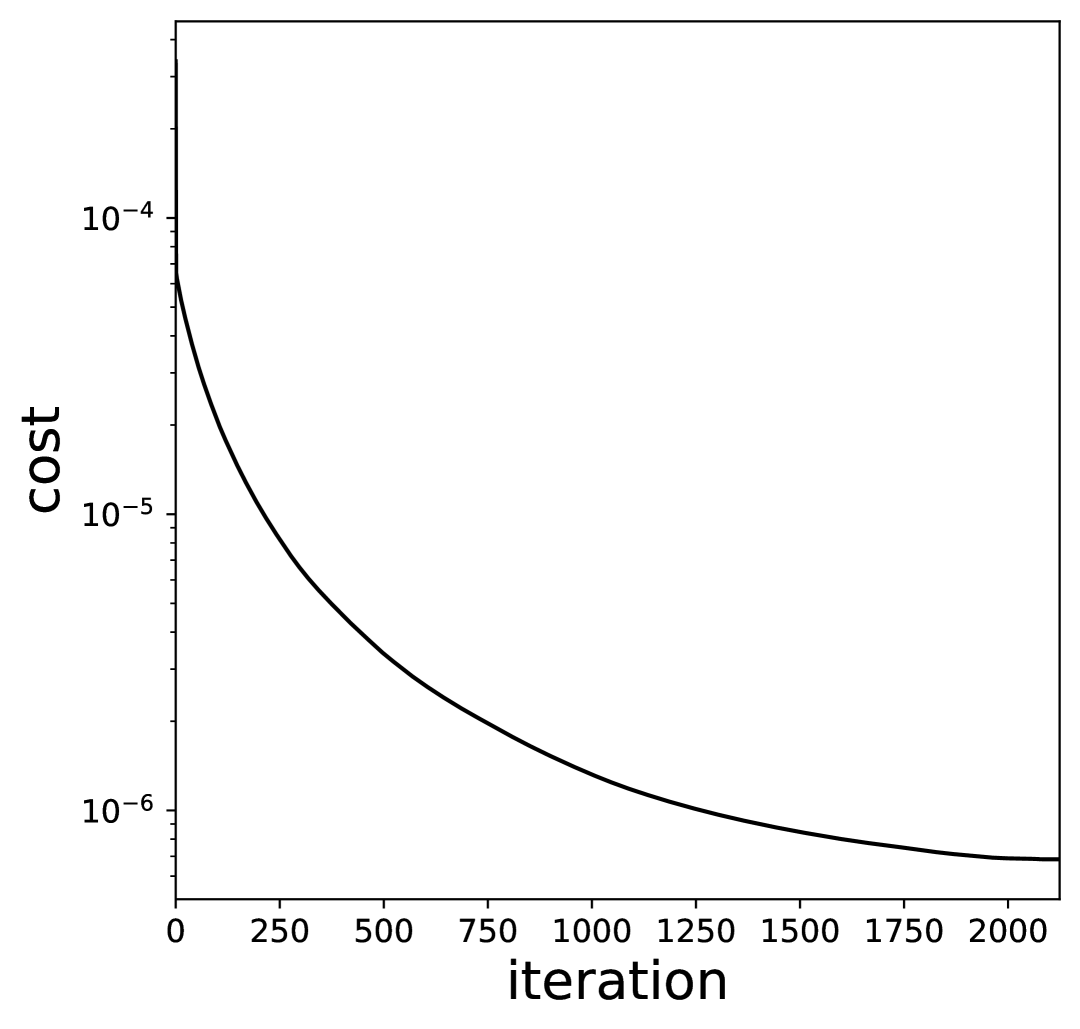
Figure 19. Results for a peanut-shape boundary interface with source $f$ (given by (39) with $\epsilon=0.3$) near the boundary, under exact (top row) and noisy measurements. Perimeter penalization was applied in all of the cases with $\rho_{1}=0.00003$.

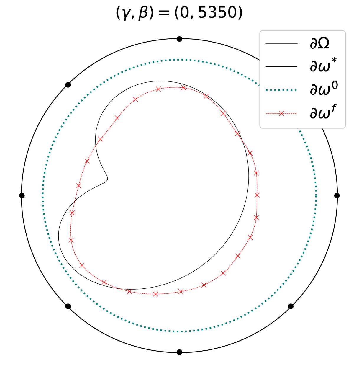
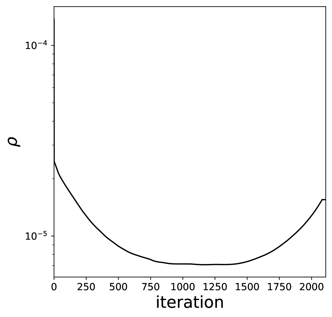
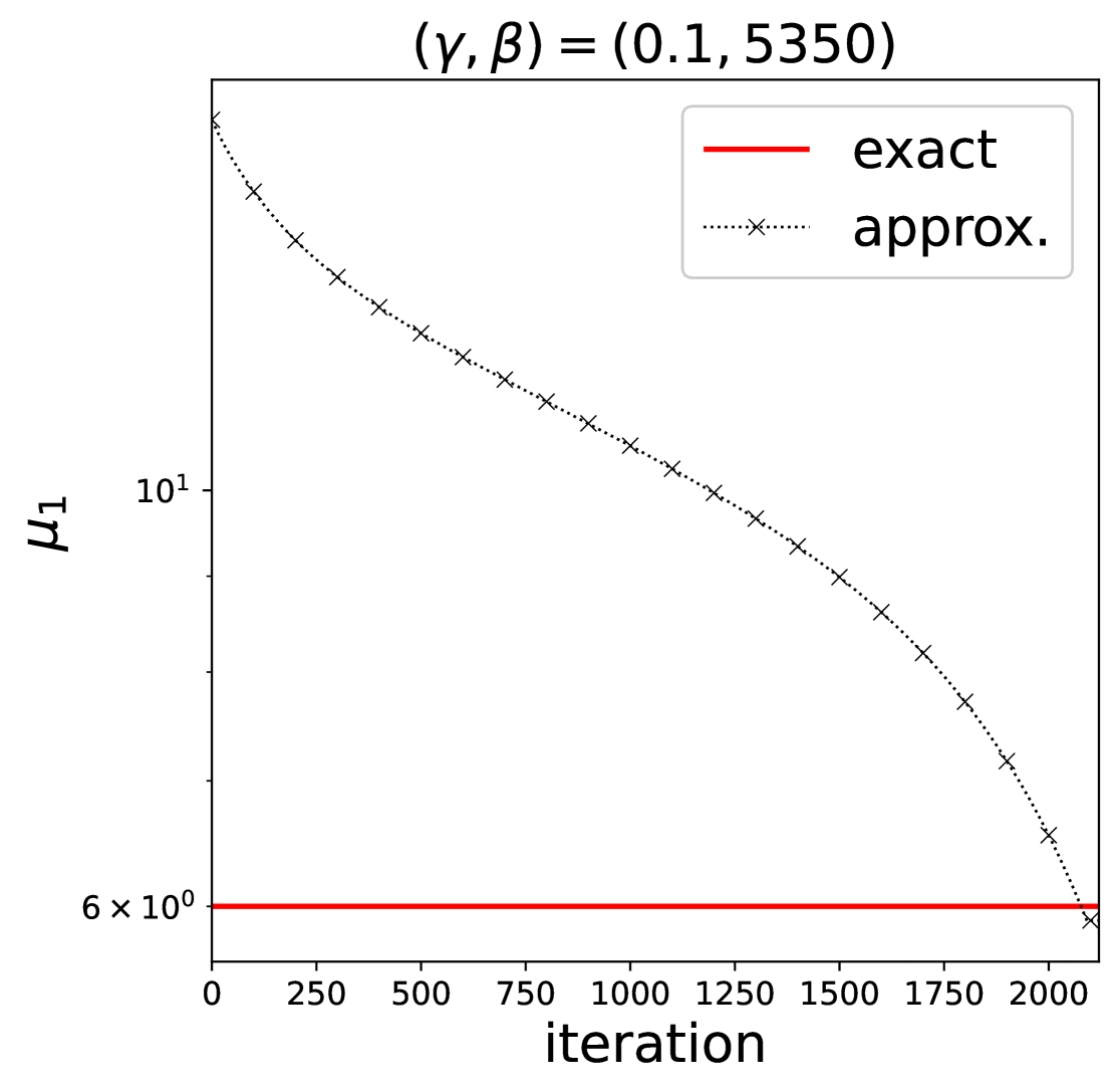
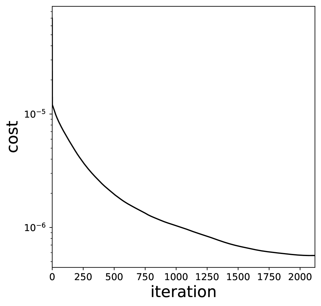
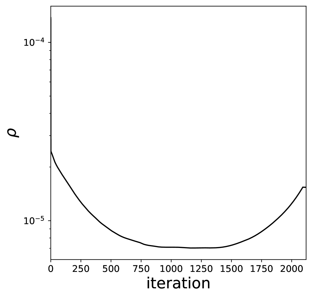
Figure 20. Results for a peanut-shape boundary interface with source $f$ (given by (39) with $\epsilon=0.2$) near the boundary, under exact (top row) and noisy measurements. The locations of the point sources are marked by thick black dots. Perimeter penalization was applied in all of the cases with $\rho_{1}=0.00003$.

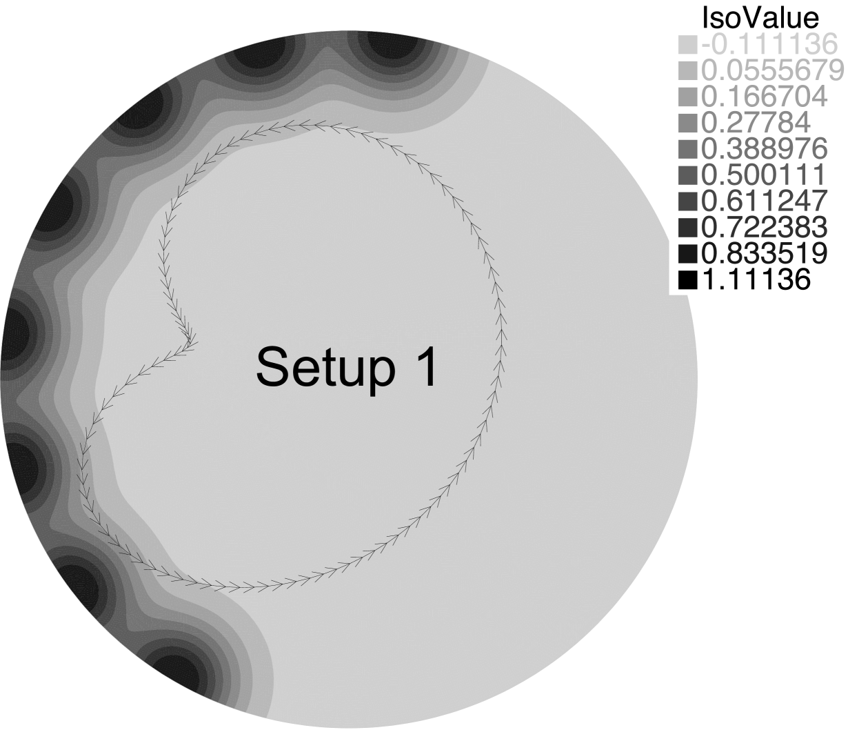
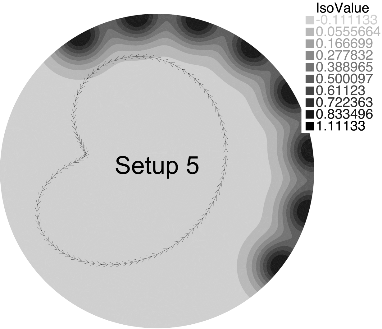
Figure 21. Positioning of sources

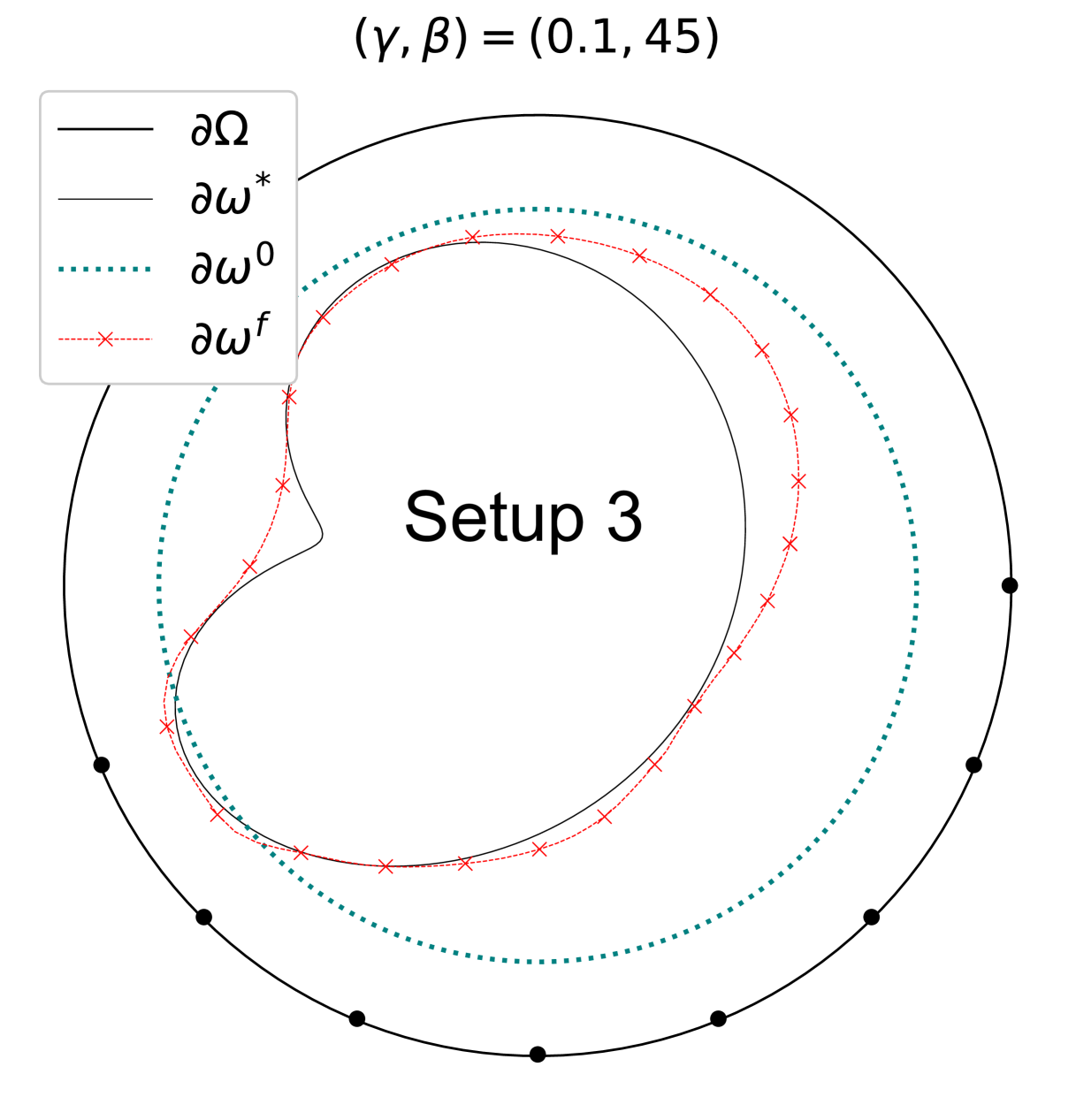
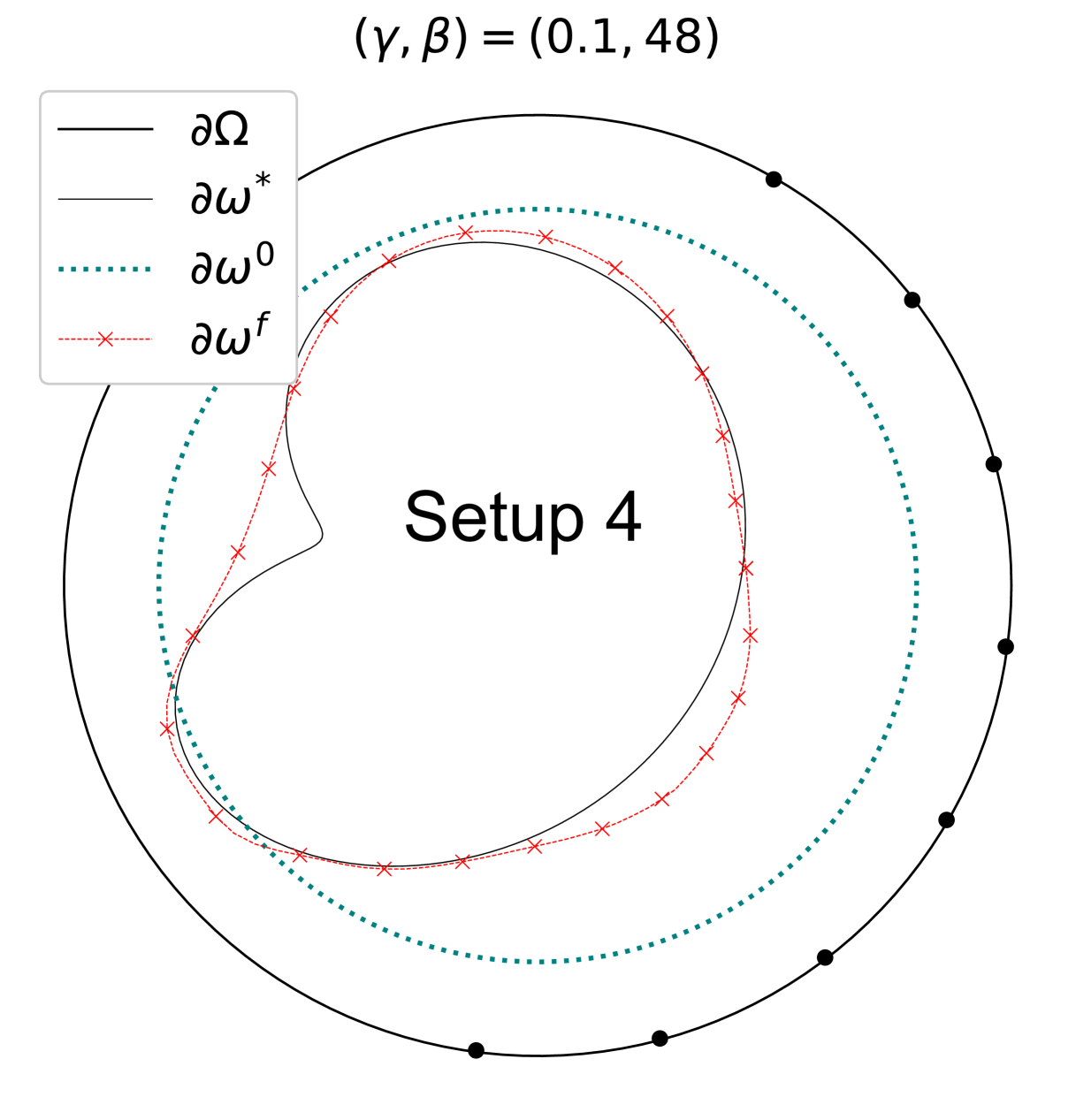
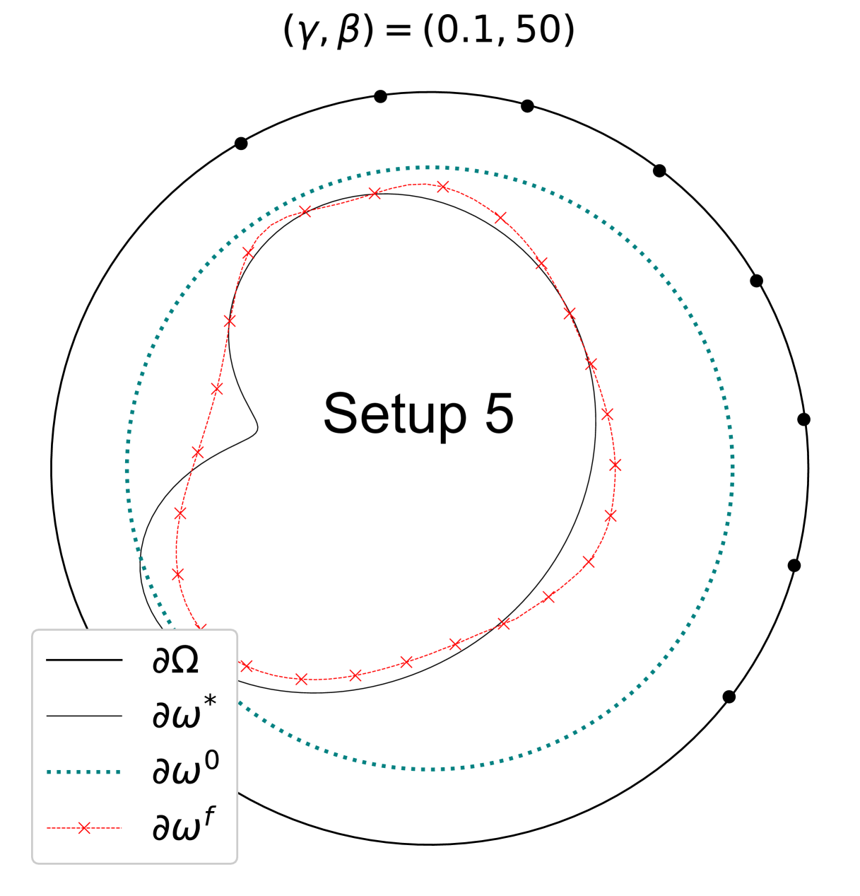
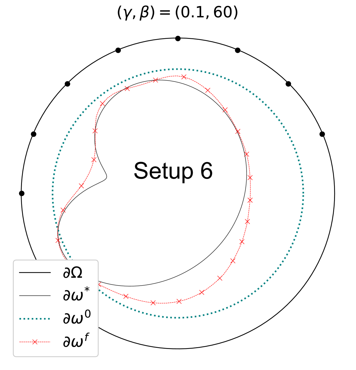
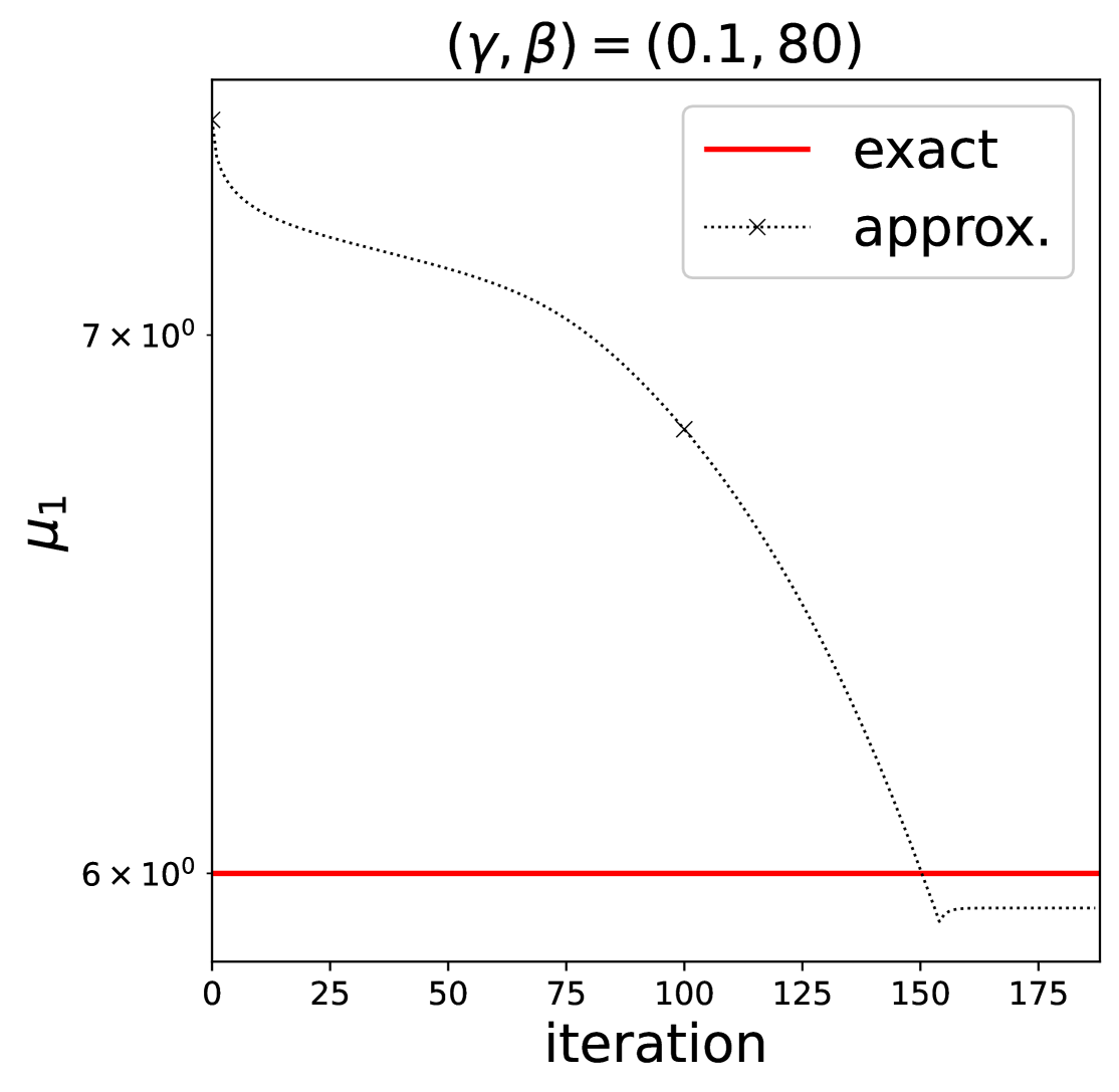
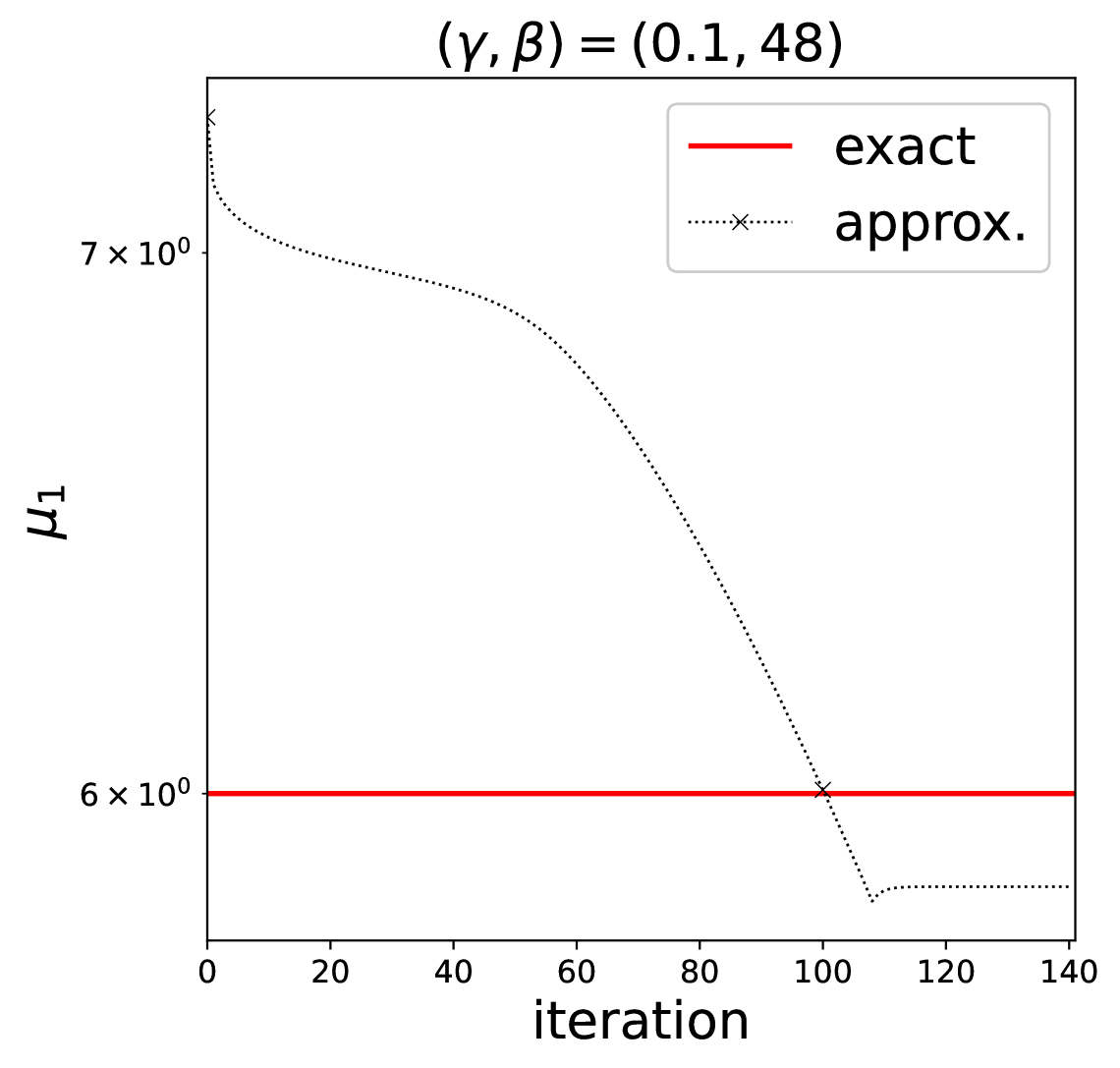
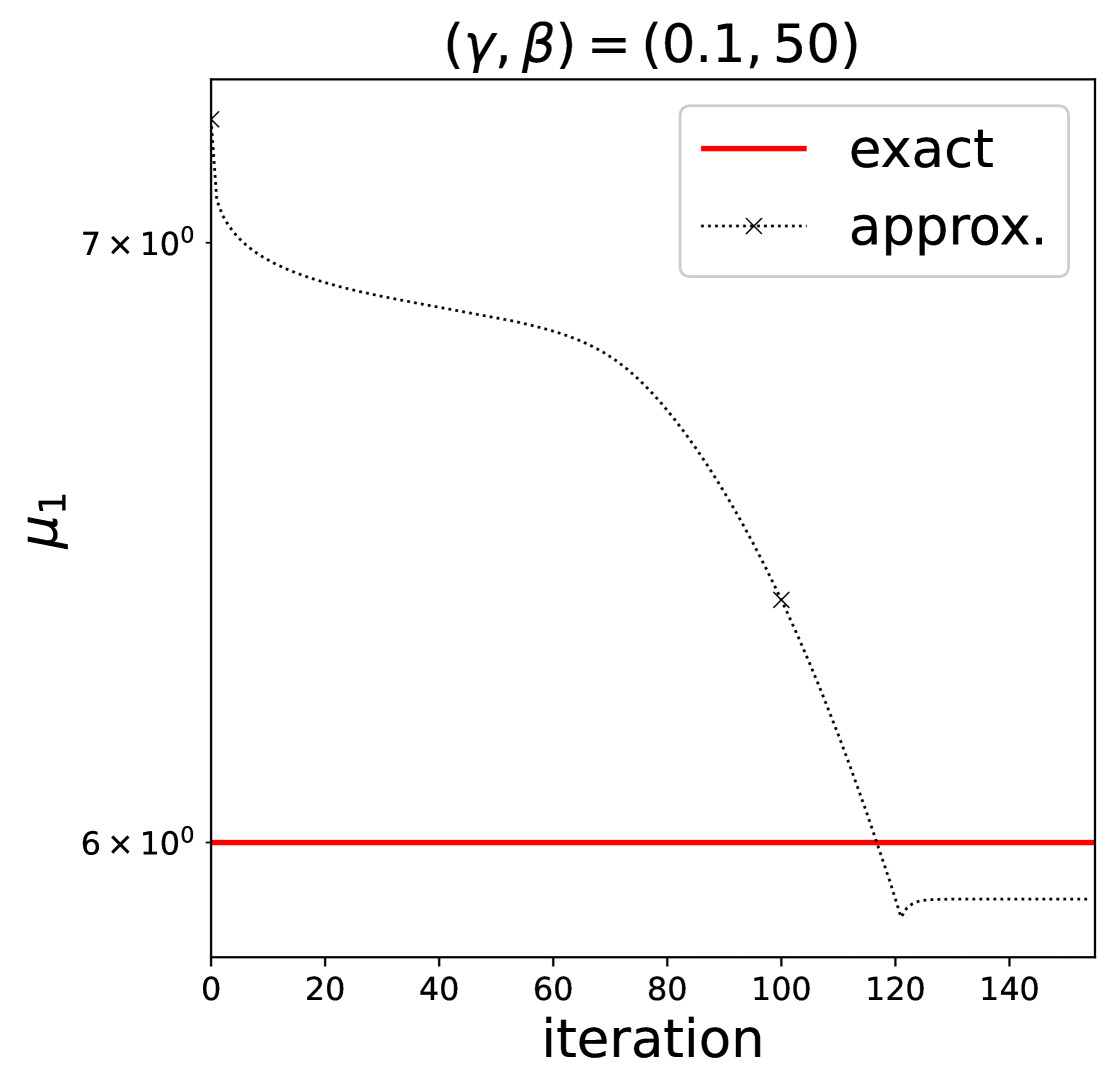
Figure 22. Results for a peanut-shape boundary interface with $f$ (given by (39) with $\epsilon=0.5$) of various positions and under noisy measurements. Perimeter penalization was applied in all of the cases with $\rho_{1}=0.000006$.

5. Conclusion

This study introduces a shape-optimization-based approach to tackle the complex, ill-posed problem of space-dependent parameter reconstruction in inverse diffusion problems. By reconstructing the constant $\mu$ and the boundary interface with only one boundary measurement, we demonstrated the versatility and robustness of this method, particularly in scenarios involving non-smooth, non-convex boundaries. Despite the difficulties in precisely capturing boundary vertices and edges, the method reliably reconstructs $\mu$ and accurately identifies concave features of the boundary interface, even under noisy conditions. The influence of point source placement on reconstruction accuracy, especially in concave regions, highlights an expected spatial sensitivity. Overall, the results confirm that the proposed approach is practical and effective for complex boundary interface reconstructions, emphasizing its applicability to various related reconstruction problems that focus on parameter identification with jump discontinuities. A key insight of the method is its non-trivial nature, as achieving an accurate reconstruction depends on a carefully chosen parameter $\beta$.

In follow-up work, we will focus on stability analysis when the primary quantity of interest is the jump in the absorption coefficient. Specifically, we will derive a local stability estimate for a parameterized, non-monotone family of domains and provide a quantitative stability result for the local optimal solution under perturbations of the absorption coefficient parameter. This investigation will extend the current formulation by incorporating both the first-order and second-order shape derivatives of the cost functional, offering a deeper understanding of the method’s robustness. Additionally, exploring other objective functionals, including the well-known Kohn-Vogelius cost functional [KV84, Mef21], will be the focus of future investigations.

Harrach showed that two parameters can be uniquely determined using the time-independent diffusion equation (1) if the diffusion coefficient is piecewise constant and the absorption coefficient is piecewise analytic [Har09]. In this sense, the approach developed in this paper can be applied to the simultaneous reconstruction of two parameters.

In addition to DOT, the present method can potentially be applied to other optical imaging techniques, such as fluorescence DOT (FDOT) (see [Jia10, p. 165], [MOW⁺03, MP03], and [DCBY12]), ultrasound-modulated fluorescence techniques [Liu14], and fluorescence molecular tomography (FMT) [NTBW02].

Appendix A Appendices

A. Proofs of some auxiliary results

A.1. Well-posedness of the state

Proof of Lemma 2.3.

The proof follows from Lax-Milgram lemma. Indeed, it can be shown that the following inequalities hold:

$$\left|{a(u,v)}\right| \leqslant\max\{{\alpha},\mu_{\max},\zeta^{-1}\}\left\|{u}\right\|_{V}\left\|{|v}\right\|_{V},\quad(u,v\in V);$$

(A.40) $$a(u,u) \geqslant\min\{{\alpha},\mu_{\min}\}\left\|{u}\right\|_{V}^{2},\quad(u\in V);$$

$$l(v) \leqslant c_{f}\left\|{v}\right\|_{V},\quad c_{f}:=\left\|{f}\right\|_{H^{-1}(\Omega)},\quad(v\in V).$$

The last two inequalities imply that

(A.41) $$\left\|{u}\right\|_{V}\leqslant c_{b}c_{f},\quad c_{b}:=\frac{1}{\min\{{\alpha},\mu_{\min}\}}>0.$$

The rest of the arguments are standard, so we omit it. ∎

A.2. Continuity of the parameter-to-state map

Proof of Proposition 2.4.

Let us write

(A.42) $$a(\mu,u,v)=\int_{\Omega}{({\alpha}\nabla{u}\cdot\nabla{v}+{\mu}{u}{v})}{\,{d}x}+\frac{1}{\zeta}\int_{\partial\Omega}{{u}{v}}{\,{d}{s}},\quad\mu\in A,u,v\in{V}.$$

Now, since $\tilde{u}=F(\tilde{\mu})$ and $\accentset{\approx}{u}=F(\accentset{\approx}{\mu})$, then, clearly, we have $a(\tilde{\mu},\tilde{u},v)=l(v)=a(\accentset{\approx}{\mu},\accentset{\approx}{u},v)$, for all $v\in V$. We let $w=w(x)=\tilde{u}(x)-\accentset{\approx}{u}(x)\in V$. It can easily be verified that

$$\left\{\begin{aligned} -\operatorname{div}{\left({\alpha}\nabla{w}\right)}+\tilde{\mu}{w}&=-(\tilde{\mu}-\accentset{\approx}{\mu})\accentset{\approx}{u},\quad\text{in }\Omega,\\ {\alpha}\partial_{\bm{\mathbf{n}}}{w}+\frac{1}{\zeta}w&=0,\quad\text{on }\partial\Omega.\end{aligned}\right.$$

Using $a$ in (A.42), we have the variational equation $a(\tilde{\mu},u,v)=-((\tilde{\mu}-\accentset{\approx}{\mu})\accentset{\approx}{u},v)_{\Omega}$, for all $v\in V$. We set $v=w$ and apply (A.40) and the Cauchy-Schwarz inequality to get

$$\min\{{\alpha},\mu_{\min}\}\left\|{w}\right\|_{V}^{2}\leqslant\left\|{\tilde{\mu}-\accentset{\approx}{\mu}}\right\|_{L^{\infty}(\Omega)}\left\|{\accentset{\approx}{u}}\right\|_{L^{2}(\Omega)}\left\|{w}\right\|_{L^{2}(\Omega)}\leqslant\left\|{\tilde{\mu}-\accentset{\approx}{\mu}}\right\|_{L^{\infty}(\Omega)}\left\|{\accentset{\approx}{u}}\right\|_{V}\left\|{w}\right\|_{V}.$$

Employing estimate (A.41), we obtain

(A.43) $$\left\|{w}\right\|_{V}\leqslant c_{b}^{2}c_{f}\left\|{\tilde{\mu}-\accentset{\approx}{\mu}}\right\|_{L^{\infty}(\Omega)}.$$

Taking $c=c_{b}^{2}c_{f}\left\|{\tilde{\mu}-\accentset{\approx}{\mu}}\right\|_{L^{\infty}(\Omega)}$ concludes the proof. ∎

A.3. Differentiability of the operator $F$

Proof of Proposition 2.5.

Let $u\in V$ be the unique solution to Problem 2.2. Then, the existence of a unique weak solution to the variational equation (9) can be verified easily using the Lax-Milgram lemma. We omit the proof since the argumentations are standard.

We subtract (9) from (7) to obtain $a(\mu,{\delta{w}}-\delta{u},v)=-(\nu{\delta{w}},v)_{\Omega}$, for all $v\in V$. Taking $v={\delta{w}}-\delta{u}$, we obtain – appealing to (A.40) and employing Cauchy-Schwarz inequality – the estimate $\min\{{\alpha},\mu_{\min}\}\left\|{{\delta{w}}-\delta{u}}\right\|_{V}^{2}=-(\nu{\delta{w}},{\delta{w}}-\delta{u})_{\Omega}\leqslant\left\|{\nu}\right\|_{L^{\infty}(\Omega)}\left\|{{\delta{w}}}\right\|_{V}\left\|{{\delta{w}}-\delta{u}}\right\|_{V}.$ Consequently, we get $\left\|{{\delta{w}}-\delta{u}}\right\|_{V}\leqslant c_{b}\left\|{\nu}\right\|_{L^{\infty}(\Omega)}\left\|{{\delta{w}}}\right\|_{V}$. In view of (A.43) and with respect to (6), we find that $\left\|{{\delta{w}}}\right\|_{V}\leqslant c_{b}^{2}c_{f}\left\|{\nu}\right\|_{L^{\infty}(\Omega)}$. Combining the last two estimates lead us to $\left\|{{\delta{w}}-\delta{u}}\right\|_{V}\leqslant c_{b}^{3}c_{f}\left\|{\nu}\right\|_{L^{\infty}(\Omega)}^{2}$. This yields

(A.44) $$\dfrac{\left\|{F(\mu+\nu)-F(\mu)-\delta{u}}\right\|_{V}}{\left\|{\nu}\right\|_{L^{\infty}(\Omega)}}\leqslant\dfrac{\left\|{{\delta{w}}-\delta{u}}\right\|_{V}}{\left\|{\nu}\right\|_{L^{\infty}(\Omega)}}\leqslant c_{b}^{3}c_{f}\left\|{\nu}\right\|_{L^{\infty}(\Omega)}.$$

In conclusion, $F$ is differentiable at $\mu$ and $DF(\mu)\nu=\delta{u}$.

Now, let us take $v=\delta{u}\in{V}$ in (9). Then, again, in view of (A.43) and by the Cauchy-Schwarz inequality, we get $\min\{{\alpha},\mu_{\min}\}\left\|{\delta{u}}\right\|_{V}^{2}\leqslant\left|{a(\mu,\delta{u},\delta{u})}\right|=\left|{(\nu u,\delta{u})_{\Omega}}\right|\leqslant\left\|{\nu}\right\|_{L^{\infty}(\Omega)}\left\|{u}\right\|_{V}\left\|{\delta{u}}\right\|_{V}\leqslant c_{b}c_{f}\left\|{\nu}\right\|_{L^{\infty}(\Omega)}\left\|{\delta{u}}\right\|_{V}.$ This leads to the inequality

(A.45) $$\left\|{\delta{u}}\right\|_{V}\leqslant c,\qquad c=c_{b}^{2}c_{f}\left\|{\nu}\right\|_{{\infty}}.$$

Thus, it follows that $DF(\mu)$ is uniformly bounded, thereby concluding the proof. ∎

A.4. Second-order sensitivity analysis

Proof of Proposition 2.6.

The well-posedness of (9) in Proposition 2.5 implies the existence of unique solution $\delta^{2}{u}\in V$ to (11) by Lax-Milgram lemma. The proof is standard so we omit it.

Now, we subtract (11) from (10) to obtain $a(\mu+\nu_{1},{\delta^{2}{w}},v)-a(\mu,\delta^{2}{u},v)=-(\nu_{2}[F(\mu+\nu_{1})-F(\mu)-DF(\mu)\nu_{1}],v)_{\Omega}$, for all $v\in V$, or equivalently, after rearrangement,

$$a(\mu,{\delta^{2}{w}}-\delta^{2}{u},v)=-(\nu_{2}[F(\mu+\nu_{1})-F(\mu)-DF(\mu)\nu_{1}],v)_{\Omega}-(\nu_{1}{\delta^{2}{w}},v)_{\Omega},\quad\forall v\in V.$$

By taking $v=z:={\delta^{2}{w}}-\delta^{2}{u}$ and then employing the Cauchy-Schwarz inequality as well as the coercivity of the bilinear form $a$ (cf. (A.40)), we obtain

(A.46) $$\frac{1}{c_{b}}\left\|{z}\right\|_{V}^{2} \leqslant\left\|{\nu_{2}}\right\|_{L^{\infty}(\Omega)}\left\|{F(\mu+\nu_{1})-F(\mu)-DF(\mu)\nu_{1}}\right\|_{V}\left\|{z}\right\|_{V}+\left\|{\nu_{1}}\right\|_{L^{\infty}(\Omega)}\left\|{\delta^{2}{w}}\right\|_{V}\left\|{z}\right\|_{V}.$$

Utilizing estimates (A.44) and (A.45) – employing similar argumentations while noting (A.43) – we have

$$\left\|{F(\mu+\nu_{1})-F(\mu)-DF(\mu)\nu_{1}}\right\|_{V}\leqslant c_{b}^{3}c_{f}\left\|{\nu_{1}}\right\|_{L^{\infty}(\Omega)}^{2}\quad\text{and}\quad\left\|{\delta^{2}{w}}\right\|_{V}\leqslant c_{b}^{3}c_{f}\left\|{\nu_{1}}\right\|_{L^{\infty}(\Omega)}\left\|{\nu_{2}}\right\|_{L^{\infty}(\Omega)}.$$

With these estimates, we deduce from (A.46) the following bound $\left\|{z}\right\|_{V}^{2}\leqslant c_{b}^{3}c_{f}\left\|{\nu_{1}}\right\|_{L^{\infty}(\Omega)}^{2}\left\|{\nu_{2}}\right\|_{L^{\infty}(\Omega)}$, from which we obtain the estimate

(A.47) $$\dfrac{\left\|{DF(\mu+\nu_{1})\nu_{2}-DF(\mu)\nu_{2}-\delta^{2}{u}}\right\|_{V}}{\left\|{\nu_{1}}\right\|_{L^{\infty}(\Omega)}}\leqslant\dfrac{\left\|{{\delta^{2}{w}}-\delta^{2}{u}}\right\|_{V}}{\left\|{\nu_{1}}\right\|_{L^{\infty}(\Omega)}}\leqslant c_{b}^{3}c_{f}\left\|{\nu_{1}}\right\|_{L^{\infty}(\Omega)}\left\|{\nu_{2}}\right\|_{L^{\infty}(\Omega)}.$$

This shows that $F$ is twice-differentiable at $\mu$ and $\delta^{2}{u}=D^{2}F(\mu)[\nu_{1},\nu_{2}]$.

Now, choosing $v=\delta^{2}{u}$ in (11), and then utilizing estimate (A.45), we obtain

(A.48) $$\left\|{\delta^{2}{u}}\right\|_{V}\leqslant c_{b}^{3}c_{f}\left\|{\nu_{1}}\right\|_{L^{\infty}(\Omega)}\left\|{\nu_{2}}\right\|_{L^{\infty}(\Omega)}.$$

Choosing $c=c_{b}^{3}c_{f}\left\|{\nu_{1}}\right\|_{L^{\infty}(\Omega)}\left\|{\nu_{2}}\right\|_{L^{\infty}(\Omega)}$, we conclude that $D^{2}F(\mu)$ is uniformly bounded. This proves the proposition. ∎

A.5. Strict convexity of the regularized functional

Proof of Proposition 2.9.

For brevity, we write $u=u(\mu)$. Observe that the first and the third term of $J_{\rho}^{\prime\prime}(\mu)[\nu,\nu]$ are non-negative, hence, we only need to examine the second term. We claim that it is positive. In view of (A.41) and (A.48), together with the trace theorem, we get

$$\left|{\left\langle{u{}},{\delta^{2}{u}}\right\rangle_{\partial\Omega}}\right|\leqslant\left\|{u{}}\right\|_{L^{2}(\partial\Omega)}\left\|{\delta^{2}{u}}\right\|_{L^{2}(\partial\Omega)}\lesssim\left\|{u{}}\right\|_{L^{2}(\Omega)}\left\|{\delta^{2}{u}}\right\|_{L^{2}(\Omega)} \leqslant c_{b}^{3}c_{f}\left\|{u{}}\right\|_{V}\left\|{\nu}\right\|_{L^{\infty}(\Omega)}^{2}$$

$$\leqslant c_{b}^{4}c_{f}^{2}\left\|{\nu}\right\|_{L^{\infty}(\Omega)}^{2}.$$

Let $\rho_{0}=c_{b}^{4}c_{f}^{2}>0$. Invoking our key assumption (2.7), we get the following lower estimate

$$J_{\rho}^{\prime\prime}(\mu)[\nu,\nu]\geqslant\left\|{\delta{u}}\right\|_{L^{2}(\partial\Omega)}^{2}-\left|{\left\langle{u{}},{\delta^{2}{u}}\right\rangle_{\partial\Omega}}\right|+\rho\left\|{\nu}\right\|_{L^{2}(\Omega)}^{2}\\ \geqslant\left\|{\delta{u}}\right\|_{L^{2}(\partial\Omega)}^{2}+(\rho-\rho_{0})\left\|{\nu}\right\|_{L^{\infty}(\Omega)}^{2}.$$

Clearly, choosing $\rho>\rho_{0}>0$, we get $J_{\rho}^{\prime\prime}(\mu)[\nu,\nu]>0$ – proving that $J_{\rho}$ is strictly convex. ∎

B. Computation of the material and shape derivatives of the state

Proof of Theorem 3.3.

The proof consists of two primary steps: first, we characterize the material derivative of the state, followed by the derivation of the shape derivative of the state; see [ADK07] for a closely related derivation in the context of a transmission problem.

First step: Let $u_{t}=u(\omega_{t})$, where $t\in\textsf{I}$, and $\Omega\in\mathcal{O}_{ad}^{k}$, satisfying (2.2). To prove the given proposition, we first show the existence of the material derivative $\dot{u}$ of $u$ which is defined as follows (see, e.g., [SZ92, Eq. (3.38), p. 111]):

(B.49) $$\dot{u}=\dot{u}(\Omega)[\bm{\mathbf{\theta}}]=\lim_{t\searrow 0}\frac{u(\Omega_{t})\circ T_{t}-u(\Omega)}{t}$$

provided the limit $\dot{u}$ exists in $H^{1}(\Omega)$ where $(u(\Omega_{t})\circ T_{t})(x)=u(\Omega_{t})(T_{t}(x))$, $x\in\Omega$.

Let us consider $u_{t}\in V_{t}:=H^{1}(\Omega_{t})$, the solution of the perturbed problem for a given variation $\bm{\mathbf{\theta}}\in{{\mathsf{\Theta}}^{k}}$ given by the solution of

(B.50) $$a_{t}(u_{t},v_{t})=l_{t}(v_{t}),\quad\forall v_{t}\in V_{t}.$$

where

$$\left\{\begin{aligned} a_{t}(u_{t},v_{t})&=\int_{\Omega_{t}}{({\alpha_{t}}\nabla{u_{t}}\cdot\nabla{v_{t}}+{\mu_{t}}{u_{t}}{v_{t}})}{\,{d}x_{t}}+\frac{1}{\zeta}\int_{\partial\Omega_{t}}{{u_{t}}{v_{t}}}{\,{d}{s}_{t}},\quad\text{for }u_{t},v_{t}\in V_{t},\\ l_{t}(v_{t})&=\int_{\Omega_{t}}{f_{t}v_{t}}{\,{d}x_{t}},\quad\text{for }v_{t}\in{V_{t}}.\end{aligned}\right.$$

Here, $\alpha_{t}$, $\mu_{t}$, and $f_{t}$ are defined as $\alpha$, $\mu$, and $f$ but replacing $\Omega$ by the perturbed domain $\Omega_{t}$, and the gradient, $\nabla$, is taken with respect to the spatial variable $x\in\Omega$.

By applying the change of variables (cf. [DZ11, subsec. 9.4.2–9.4.3, pp. 482–484]), one can write equation (B.50) as follows:

(B.51) $$a^{t}(u^{t},v)=l^{t}(v),\quad\forall v\in V,$$

where

$$\left\{\begin{aligned} a^{t}(u^{t},v)&=\int_{\Omega}{({\alpha^{t}}A_{t}\nabla{u^{t}}\cdot\nabla{v}+I_{t}{\mu^{t}}{u^{t}}{v})}{\,{d}x}+\frac{1}{\zeta}\int_{\partial\Omega}{b_{t}{u^{t}}{v}}{\,{d}{s}},\quad\text{for }u^{t},v\in V,\\ l^{t}(v)&=\int_{\Omega}{I_{t}f^{t}v}{\,{d}x},\quad\text{for }v\in{V},\quad(\varphi^{t}=\varphi_{t}\circ T_{t}:\Omega\to\mathbb{R}).\end{aligned}\right.$$

Here, observe that $b_{t}=I_{t}\left|{({D}T_{t})^{-\top}\bm{\mathbf{n}}}\right|=1$ because $\bm{\mathbf{\theta}}$ vanishes on $\partial\Omega$.

Now, for all $t\in[0,t_{0})$, with $t_{0}$ sufficiently small, one can show that $w^{t}=u^{t}-u\in V$ is a unique solution to the variational equation $a^{t}(u^{t},v)-a(u,v)=l^{t}(v)-l(v)$, for all $v\in V$, which can equivalently be written as

(B.52) $$\tilde{a}(w^{t},v)=\tilde{l}(v),\quad\forall v\in V,$$

where

(B.53) $$\left\{\begin{aligned} \tilde{a}(w^{t},v)&=\int_{\Omega}{({\alpha^{t}}\nabla{w^{t}}\cdot\nabla{v}+{\mu^{t}}{w^{t}}{v})}{\,{d}x}+{\frac{1}{\zeta}\int_{\partial\Omega}{{w^{t}}{v}}{\,{d}{s}}},\quad\text{for }w^{t},v\in V,\\ \tilde{l}(v)&=-\int_{\Omega}{(\alpha^{t}-\alpha)A_{t}\nabla{u^{t}}\cdot\nabla{v}}{\,{d}x}-\int_{\Omega}{\alpha(A_{t}-id)\nabla{u^{t}}\cdot\nabla{v}}{\,{d}x}\\ &\qquad-\int_{\Omega}{I_{t}(\mu^{t}-\mu){u^{t}}{v}}{\,{d}x}-\int_{\Omega}{(I_{t}-1)\mu{u^{t}}{v}}{\,{d}x}\\ &\qquad+\int_{\Omega}{I_{t}(f^{t}-f){v}}{\,{d}x}+\int_{\Omega}{(I_{t}-1)f{v}}{\,{d}x},\quad\text{for }u^{t},v\in V.\\ \end{aligned}\right.$$

The well-posedness of (B.52) essentially follows from the Lax-Milgram theorem, by applying standard arguments and noting that $\lim_{t\searrow 0}A_{t}=\text{id}$ and $\lim_{t\searrow 0}I_{t}=1$ uniformly on ${\Omega}$, as well as the regularity assumptions on $\mu$ and $f$ given in Assumption 3.2. As a consequence, one can deduce that $\left\|{w^{t}}\right\|_{V}\lesssim\left\|{u}\right\|_{V}$ ($t\in\textsf{I}=[0,t_{0})$). This means that the set $\{w^{t}\mid t\in\textsf{I}\}$ is bounded in $V$ for sufficiently small $t_{0}$.

Let us define $z^{t}=\frac{1}{t}w^{t}$ for $t\in(0,t_{0})$ which also belongs to $V$. Then, we have

(B.54) $$\tilde{a}(z^{t},v) =-\int_{\Omega}{\left(\dfrac{\alpha^{t}-\alpha}{t}\right)A_{t}\nabla{u^{t}}\cdot\nabla{v}}{\,{d}x}-\int_{\Omega}{\alpha\left(\dfrac{A_{t}-id}{t}\right)\nabla{u^{t}}\cdot\nabla{v}}{\,{d}x}$$

$$\quad-\int_{\Omega}{I_{t}\left(\dfrac{\mu^{t}-\mu}{t}\right){u^{t}}{v}}{\,{d}x}-\int_{\Omega}{\left(\dfrac{I_{t}-1}{t}\right)\mu{u^{t}}{v}}{\,{d}x}$$

$$\quad+\int_{\Omega}{I_{t}\left(\dfrac{f^{t}-f}{t}\right){v}}{\,{d}x}+\int_{\Omega}{\left(\dfrac{I_{t}-1}{t}\right)f{v}}{\,{d}x}=\frac{1}{t}\tilde{l}(v)=:l_{t}(v),\quad(\forall v\in V).$$

By selecting $v=z^{t}$ as the test function in the equation above, we can infer the boundedness of the sequence $\{z^{t}\}$ in $V$. Specifically, we consider a sequence $\{t_{n}\}$ such that $\lim_{n\to\infty}t_{n}=0$, and our goal is to demonstrate that $\lim_{n\to\infty}z^{t_{n}}$ exists. The properties of the transformation $T_{t}$ given in (23), together with the boundedness of $w^{t}$ in $V$ implies that $\nabla z^{t}$ is bounded in $L^{2}(\Omega)^{d}$, equivalently the sequence $\{z^{t_{n}}\}$ is bounded in $V$. Thus, there is a subsequence, which we still denote by $t_{n}$ with $t_{n}\searrow 0$ and an element $z\in V$ such that $z^{t_{n}}\rightharpoonup z$ weakly in $V$. Since $\nabla u^{t_{n}}\to\nabla u$ in $L^{2}(\Omega)^{d}$, $\lim_{t_{n}\searrow 0}{I}_{t_{n}}=1$ and $\lim_{t_{n}\searrow 0}A_{t_{n}}=id$ uniformly on $\Omega$, and the derivatives of the maps $[t\mapsto I_{t}]$ and $[t\mapsto A_{t}]$ given in (24) we get

(B.55) $$a_{0}(z,v) :=\int_{\Omega}{({\alpha\nabla{z}\cdot\nabla{v}+{\mu}{z}{v})}}{\,{d}x}+{\frac{1}{\zeta}\int_{\partial\Omega}{{z}{v}}{\,{d}{s}}}$$

$$=-\int_{\Omega}{\left(\nabla{\alpha}\cdot\bm{\mathbf{\theta}}(\nabla{u}\cdot\nabla{v})+\alpha A\nabla{u}\cdot\nabla{v}\right)}{\,{d}x}-\int_{\Omega}{\left(\nabla{\mu}\cdot\bm{\mathbf{\theta}}{u}{v}+\operatorname{div}{\bm{\mathbf{\theta}}}\mu{u}{v}\right)}{\,{d}x}$$

$$\qquad+\int_{\Omega}{\left(\nabla{f}\cdot\bm{\mathbf{\theta}}{v}+\operatorname{div}{\bm{\mathbf{\theta}}}f{v}\right)}{\,{d}x}$$

$$=:j_{1}(v)+j_{2}(v)+j_{3}(v)=:l_{0}(v),\qquad(\forall v\in V).$$

In above, the limit equation

(B.56) $$\lim_{t\to 0}\frac{1}{t}\left(I_{t}\varphi^{t}-\varphi\right)=\operatorname{div}(\varphi\bm{\mathbf{\theta}})=\varphi\operatorname{div}{\bm{\mathbf{\theta}}}+\nabla{\varphi}\cdot\bm{\mathbf{\theta}}$$

was used which holds for any differentiable mapping $t\mapsto I_{t}\varphi^{t}$ from interval I to $L^{2}(\Omega)$ with $\varphi\in V$ and $\bm{\mathbf{\theta}}\in{{\mathsf{\Theta}}^{k}}$ (cf. [IKP06, Cor. 3.1]). Since this equation has a unique solution, we deduce the weak convergence $z^{t_{n}}\rightharpoonup z$ in $V$ for any sequence $\{t_{n}\}$. Meanwhile, the strong convergence follows from the fact that $a_{0}(z,z)=\lim_{t_{n}\searrow 0}\tilde{a}({z^{t_{n}}},{z^{t_{n}}})=\lim_{t_{n}\searrow 0}l_{t_{n}}({z^{t_{n}}})=l_{0}(v).$ together with the weak convergence previously shown. This proves the characterization of the (unique) material derivative $z=\dot{u}\in V$ of $u\in V$ given in equation (26).

Second step: Next, we shall derive the structure of the shape derivative of the state. First, we recall that the function $u$ has a shape derivative $u^{\prime}$ at $0$ in the direction of the vector field $\bm{\mathbf{\theta}}\in{{\mathsf{\Theta}}^{k}}$ if the limit

$$u^{\prime}=\lim_{t\searrow 0}\frac{u(\Omega_{t})-u(\Omega)}{t},$$

exist. This expression and the material derivative $\dot{u}$ are related by $u^{\prime}=\dot{u}-(\nabla u\cdot\bm{\mathbf{\theta}})$ provided that $\nabla u\cdot\bm{\mathbf{\theta}}$ exists in some appropriate function space [SZ92, Eq. (3.38), p. 111]. We comment that the shape derivative $u^{\prime}$ of (1) is not continuous across the interface $\partial\omega$. As a consequence, $u^{\prime}$ cannot be in $H^{1}(\Omega)$. Nonetheless, it belongs to $H^{1}(\Omega_{+})\cup H^{1}(\Omega_{-})$.

To proceed with the derivation of $u^{\prime}$, we rewrite equation (B.55) in another form. To do so, we observe that by applying the chain rule in conjunction with (24), the following expansions and identities hold (here $u$ is restricted to $\Omega_{\pm}$):

(B.57) $$-\left(\nabla{\alpha}\cdot\bm{\mathbf{\theta}}(\nabla{u}\cdot\nabla{v})+\alpha A\nabla{u}\cdot\nabla{v}\right) =\nabla{u}\cdot\left(\alpha(D\bm{\mathbf{\theta}}+D\bm{\mathbf{\theta}}^{\top})-\operatorname{div}{(\alpha\bm{\mathbf{\theta}})}id\right)\nabla{v}$$

$$=\operatorname{div}\left(\alpha(\bm{\mathbf{\theta}}\cdot\nabla{u})\nabla{v}+{\alpha(\bm{\mathbf{\theta}}\cdot\nabla{v})\nabla{u}-\alpha(\nabla{u}\cdot\nabla{v})\bm{\mathbf{\theta}}}\right)$$

$$\qquad-(\bm{\mathbf{\theta}}\cdot\nabla{u})\operatorname{div}{(\alpha\nabla{v})}-(\bm{\mathbf{\theta}}\cdot\nabla{v})\operatorname{div}{(\alpha\nabla{u})},$$

$$\alpha\nabla(\nabla{u}\cdot\bm{\mathbf{\theta}})\cdot\nabla{v} =\alpha\nabla^{2}{u}\bm{\mathbf{\theta}}\cdot\nabla{v}+\alpha\nabla{\bm{\mathbf{\theta}}}\nabla{u}\cdot\nabla{v}$$

$$=\alpha(\nabla{v})^{\top}\nabla^{2}{u}\bm{\mathbf{\theta}}+\alpha D{\bm{\mathbf{\theta}}}\nabla{v}\cdot\nabla{u}$$

$$=\operatorname{div}{(\alpha(\bm{\mathbf{\theta}}\cdot\nabla{u})\nabla{v})}-(\bm{\mathbf{\theta}}\cdot\nabla{u})\operatorname{div}{(\alpha\nabla{v})},$$

where $\nabla{\bm{\mathbf{\theta}}}=(D\bm{\mathbf{\theta}})^{\top}={\partial{\theta}_{j}}/{\partial{x}_{i}}$ and $\nabla^{2}{u}$ denotes the Hessian of ${u}$ which is symmetric. On the other hand, taking $\nabla{v}_{\pm}\cdot\bm{\mathbf{\theta}}\in H^{1}(\Omega_{\pm})$, where $v_{\pm}\in V\cap H^{2}(\Omega_{\pm})$, $\bm{\mathbf{\theta}}\in{{\mathsf{\Theta}}^{k}}$ (i.e., $\bm{\mathbf{\theta}}=\bm{\mathbf{0}}$ in $\partial\omega$), as a test function in Problem 2.2 yields the following equation

(B.58) $$\int_{\Omega}{({\alpha}\nabla{u}\cdot\nabla{(\nabla{v}\cdot\bm{\mathbf{\theta}})}+{\mu}{u}{(\nabla{v}\cdot\bm{\mathbf{\theta}})})}{\,{d}x}=\int_{\Omega}{f(\nabla{v}\cdot\bm{\mathbf{\theta}})}{\,{d}x}.$$

Moreover, we have the following equivalent expressions

$$j_{2}(v) =-\int_{\Omega}{\operatorname{div}{(\mu{u}{v}\bm{\mathbf{\theta}})}}{\,{d}x}+\int_{\Omega}{\left(\mu(\bm{\mathbf{\theta}}\cdot\nabla{u}){v}+\mu{u}(\bm{\mathbf{\theta}}\cdot\nabla{v})\right)}{\,{d}x},$$

$$j_{3}(v) =\int_{\Omega}{\operatorname{div}{(fv\bm{\mathbf{\theta}})}}{\,{d}x}-\int_{\Omega}{f(\nabla{v}\cdot\bm{\mathbf{\theta}})}{\,{d}x}.$$

Utilizing the above identities in (B.55) with $z$ replaced by $\dot{u}_{\pm}={u^{\prime}_{\pm}}+\nabla{{u}_{\pm}}\cdot\bm{\mathbf{\theta}}\in H^{1}({\Omega}_{\pm})$ (observe that $(\nabla{u}\cdot\bm{\mathbf{\theta}})\not\in H^{1}(\Omega)$ but ${u}_{\pm}\in H^{k+1}({\Omega}_{\pm})$, $k\geqslant 2$), we get

(B.59) $$a_{0}(u^{\prime},v)+\int_{\Omega}{({\alpha\nabla{(\nabla{u}\cdot\bm{\mathbf{\theta}})}\cdot\nabla{v}+{\mu}{(\nabla{u}\cdot\bm{\mathbf{\theta}})}{v})}}{\,{d}x}$$

$$\ =\int_{\Omega}{({\alpha\nabla{(\nabla{u}\cdot\bm{\mathbf{\theta}})}\cdot\nabla{v}+{\mu}{(\nabla{u}\cdot\bm{\mathbf{\theta}})}{v})}}{\,{d}x}-\int_{\Omega}{\left[(\bm{\mathbf{\theta}}\cdot\nabla{v})\operatorname{div}{(\alpha\nabla{u})}-\mu{u}(\bm{\mathbf{\theta}}\cdot\nabla{v})+f(\nabla{v}\cdot\bm{\mathbf{\theta}})\right]}{\,{d}x}$$

$$\qquad+\int_{\Omega}{\operatorname{div}{\left(\alpha(\bm{\mathbf{\theta}}\cdot\nabla{v})\nabla{u}-\alpha(\nabla{u}\cdot\nabla{v})\bm{\mathbf{\theta}}\right)}}{\,{d}x}-\int_{\Omega}{\left[\operatorname{div}{(\mu{u}{v}\bm{\mathbf{\theta}})}-\operatorname{div}{(fv\bm{\mathbf{\theta}})}\right]}{\,{d}x}.$$

In above equation (and also in other places when no confusion arise), it should be noted that the integrals over each domain can be divided into two separate domain integrals. For example, we have

$$\int_{\Omega}{({\alpha\nabla{(\nabla{u}\cdot\bm{\mathbf{\theta}})}\cdot\nabla{v}+{\mu}{(\nabla{u}\cdot\bm{\mathbf{\theta}})}{v})}}{\,{d}x} =\int_{\Omega_{+}}{({\alpha_{+}\nabla{(\nabla{u_{+}}\cdot\bm{\mathbf{\theta}})}\cdot\nabla{v}+{\mu_{+}}{(\nabla{u_{+}}\cdot\bm{\mathbf{\theta}})}{v})}}{\,dx}$$

$$\qquad+\int_{\Omega_{-}}{({\alpha_{-}\nabla{(\nabla{u_{-}}\cdot\bm{\mathbf{\theta}})}\cdot\nabla{v}+{\mu_{-}}{(\nabla{u_{-}}\cdot\bm{\mathbf{\theta}})}{v})}}{\,dx},$$

where $\Omega_{+}=\Omega\setminus{\overline{\omega}}$ and $\Omega_{-}=\omega$.

For $\bm{\mathbf{\theta}}\in{{\mathsf{\Theta}}^{k}}$, observe that by using integration by parts, we have $-\int_{\Omega}{(\bm{\mathbf{\theta}}\cdot\nabla{v})\operatorname{div}{(\alpha\nabla{u})}}{\,{d}x}=\int_{\Omega}{\alpha\nabla{u}\cdot\nabla{(\bm{\mathbf{\theta}}\cdot\nabla{v})}}{\,{d}x}$. Then, in view of (B.58), equation (B.59) can be simplified as follows

(B.60) $$a_{0}(u^{\prime},v)=\int_{\Omega}{\left[\operatorname{div}{\left(\alpha(\bm{\mathbf{\theta}}\cdot\nabla{v})\nabla{u}-\alpha(\nabla{u}\cdot\nabla{v})\bm{\mathbf{\theta}}\right)}-\operatorname{div}{(\mu{u}{v}\bm{\mathbf{\theta}})}+\operatorname{div}{({f}{v}\bm{\mathbf{\theta}})}\right]}{\,{d}x},$$

which provides an inititial characterization of the shape derivative of the state.

To complete the proof, we express the right side of (B.60) as a boundary integral over $\partial\omega$. This is accomplished by applying the divergence theorem after partitioning the integral into two domains of integration: $\Omega\setminus\overline{\omega}$ and $\omega$. We then utilize the notation $\left[{\cdot}\right]_{\pm}$, which denotes the difference between the traces of a function at the boundary interface $\partial\omega$ as we approach from $\Omega\setminus\overline{\omega}$ and $\omega$, respectively. Specifically, by applying the divergence theorem in both $\Omega$ and $\Omega\setminus\overline{\omega}$, followed by integration by parts, we obtain

(B.61) $$\int_{\Omega}{(-\operatorname{div}{(\alpha\nabla{u^{\prime}})}+{\mu}{u^{\prime}}){v}}{\,{d}x}+{\int_{\partial\Omega}{\left(\alpha\partial_{\bm{\mathbf{n}}}{u^{\prime}}+\frac{1}{\zeta}{u^{\prime}}\right){v}}{\,{d}{s}}-\int_{\partial\omega}{\left[{\alpha\dfrac{\partial{u^{\prime}}}{\partial{\bm{\mathbf{n}}}}}\right]_{\pm}{v}}{\,{d}{s}}}$$

$$\qquad=a_{0}(u^{\prime},v)=\int_{\Omega}{({\alpha\nabla{u^{\prime}}\cdot\nabla{v}+{\mu}{u^{\prime}}{v})}}{\,{d}x}+{\frac{1}{\zeta}\int_{\partial\Omega}{{u^{\prime}}{v}}{\,{d}{s}}}$$

$$\qquad=-\int_{\partial\omega}{\left\{(\bm{\mathbf{\theta}}\cdot\nabla{v})\left[{\alpha\nabla{u}}\right]_{\pm}\cdot\bm{\mathbf{n}}-\left[{\alpha\nabla{u}}\right]_{\pm}\cdot\nabla{v}{\theta}_{n}-\left[{\mu{u}}\right]_{\pm}{v}{\theta}_{n}+\left[{f}\right]_{\pm}{v}{\theta}_{n}\right\}}{\,{d}{s}},$$

where ${\theta}_{n}=\bm{\mathbf{\theta}}\cdot\bm{\mathbf{n}}$. By comparing the left-most and right-most sides of the equation, while varying $v$ (which we assume to be sufficiently smooth–at least in $H^{2}(\Omega)$) over $\Omega=(\Omega\setminus{\overline{\omega}})\cup\omega$ and the over $\partial\Omega$, we deduce that the following equations hold at least in distributional sense:

$$\left\{\begin{aligned} -\operatorname{div}{\left({\alpha}\nabla{u^{\prime}}\right)}+\mu{u^{\prime}}&=0,\quad\text{in $\Omega\setminus\overline{\omega}$ and in $\omega$},\\ {\alpha}\partial_{\bm{\mathbf{n}}}{{u^{\prime}}}+\frac{1}{\zeta}{u^{\prime}}&=0,\quad\text{on }\partial\Omega.\end{aligned}\right.$$

We next derive the equation for $u^{\prime}$ on $\partial\omega$. First, let us note that, by elliptic regularity result, ${u}_{\pm}\in H^{k+1}({\Omega}_{\pm})$ (for $d\in\{2,3\}$). Then, for some $k\in\mathbb{N}$, $k\geqslant 2$, we have $u\in{{C}}^{1,\alpha}(\overline{\Omega}_{\pm})$, $0<\alpha\leqslant k-{d}/2$, $d\in\{2,3\}$, because of the Sobolev embedding $H^{k+1}({\Omega}_{\pm})\hookrightarrow{{C}}^{1,\alpha}(\overline{\Omega}_{\pm})$ (see, e.g., [DD12, Thm. 2.84, p. 98] or [AF03, Thm. 4.12, p. 85]). Now, because $\left[{u}\right]_{\pm}=0$ on $\partial\omega$, we have $\left[{\nabla{u}}\right]_{\pm}=\left[{(\partial{u}/\partial{\bm{\mathbf{n}}})\bm{\mathbf{n}}}\right]_{\pm}$ on $\partial\omega$; that is, $\left[{\nabla_{\tau}{u}}\right]_{\pm}=0$ on $\partial\omega$. Hence, $\left[{\dot{u}}\right]_{\pm}=0$ on $\partial\omega$, and so $\left[{u^{\prime}}\right]_{\pm}=\left[{\dot{u}}\right]_{\pm}-\left[{\nabla{u}\cdot\bm{\mathbf{\theta}}}\right]_{\pm}=-\left[{\nabla{u}\cdot\bm{\mathbf{\theta}}}\right]_{\pm}$ on $\partial\omega$. By these equations, we deduce that

$$\left[{u^{\prime}}\right]_{\pm}=-{\theta}_{n}\left[{\dfrac{\partial{u}}{\partial{\bm{\mathbf{n}}}}}\right]_{\pm}\quad\text{on }\partial\omega.$$

Next, we note that, from tangential Stokes’ formula [MS76], we have $\int_{\partial\omega}{\bm{\mathbf{\theta}}\cdot\nabla_{\tau}{\varphi}}{\,{d}{s}}=-\int_{\partial\omega}{\varphi\operatorname{div}_{\tau}{\bm{\mathbf{\theta}}}}{\,{d}{s}}$, when $\bm{\mathbf{\theta}}\cdot\bm{\mathbf{n}}=0$ (i.e., $\bm{\mathbf{\theta}}$ is a tangential field). Here, the operators $\nabla_{\tau}$ and $\operatorname{div}_{\tau}$ are respectively the tangential gradient and tangential divergence operators (see, e.g., [DZ11, HP18, SZ92]). We observe that $((\left[{\alpha\nabla{u}}\right]_{\pm}\cdot\bm{\mathbf{n}})\bm{\mathbf{\theta}}-{\theta}_{n}\left[{\alpha\nabla{u}}\right]_{\pm})\cdot\bm{\mathbf{n}}=0$ on $\partial\omega$. Hence, we can replace $\nabla{v}$ by $\nabla_{\tau}{v}$. In addition, we know that $\left[{\nabla_{\tau}{u}}\right]_{\pm}=0$ on $\partial\omega$ which implies that

$$-\int_{\partial\omega}{{\theta}_{n}\left[{\alpha}\right]_{\pm}\nabla_{\tau}{u}\cdot\nabla{v}}{\,{d}{s}} =-\int_{\partial\omega}{{\theta}_{n}\left[{\alpha\nabla{u}}\right]_{\pm}\cdot\nabla{v}}{\,{d}{s}}$$

$$=\int_{\partial\omega}{\left\{(\bm{\mathbf{\theta}}\cdot\nabla{v})\left[{\alpha\nabla{u}}\right]_{\pm}\cdot\bm{\mathbf{n}}-\left(\left[{\alpha\nabla{u}}\right]_{\pm}\cdot\nabla{v}\right){\theta}_{n}\right\}}{\,{d}{s}}$$

$$=\int_{\partial\omega}{{v}\operatorname{div}_{\tau}({\theta}_{n}\left[{\alpha}\right]_{\pm}\nabla_{\tau}{u})}{\,{d}{s}}.$$

Using this identity, we arrive at the following equation

$$\int_{\partial\omega}{\left[{\alpha\dfrac{\partial{u^{\prime}}}{\partial{\bm{\mathbf{n}}}}}\right]_{\pm}{v}}{\,{d}{s}}=\int_{\partial\omega}{\left(\operatorname{div}_{\tau}{({\theta}_{n}\left[{\alpha}\right]_{\pm}\nabla_{\tau}{u})}-\left[{\mu{u}}\right]_{\pm}{\theta}_{n}+\left[{f}\right]_{\pm}{\theta}_{n}\right){v}}{\,{d}{s}},$$

which holds for all $v\in V$. By varying $v$, we deduce that

$$\left[{\alpha\dfrac{\partial{u^{\prime}}}{\partial{\bm{\mathbf{n}}}}}\right]_{\pm}=K(u)[\bm{\mathbf{\theta}}]=\operatorname{div}_{\tau}{({\theta}_{n}\left[{\alpha}\right]_{\pm}\nabla_{\tau}{u})}-\left[{\mu{u}}\right]_{\pm}{\theta}_{n}+\left[{f}\right]_{\pm}{\theta}_{n},\qquad\text{on }\partial\omega.$$

This finally establishes the structure of the shape derivative of the state given in equation (28). For the more general structure of the shape derivative without the aforementioned continuity conditions, see Theorem 3.7. ∎

C. Existence of a shape solution

In this appendix, we address the question of the existence of an optimal solution to the optimization problem

(C.62) $$\min_{\omega\in\mathcal{O}_{\circ}^{1},\ \Omega\in\mathcal{O}_{ad}^{1}}J({\omega}).$$

To establish this existence, we must impose a key assumption regarding the regularity of the boundary interface, which is fortunately a consequence of the definition of the set of admissible domains $\mathcal{O}_{ad}^{1}$ provided in (22). For the purpose of our analysis, it suffices to assume that $\Omega$ is Lipschitz continuous, which allows us to establish the desired existence result (refer to Proposition C.5). In this section, we assume that $f\in H^{-1}(\Omega)$ and that $\alpha$ exhibits jump discontinuities at the boundary interface. Therefore, without further notice, we consider Problem 2.2 with $\alpha$ defined according to Assumption 3.5.

Because Problem 2.2 admits a unique weak solution by Lemma 2.3, we can define the map $\Omega\longmapsto{u}:={u}(\omega)$, and denote its graph by

$$\mathcal{G} =\{(\omega,{u}):\text{ $\omega\in{\mathcal{O}_{\circ}^{1}}$ and ${u}$ solves Problem~\ref{prob:weak_form_optimal_tomography}}\},$$

The primary result we aim to establish is as follows:

Theorem C.1.

The minimization problem (C.62) admits at least one solution in $\mathcal{G}$.

To demonstrate the validity of this assertion, we first need to endow the set $\mathcal{G}$ with a topology that ensures its compactness and the lower semi-continuity of the functional ${J}$. To achieve this, we introduce a topology on $\mathcal{G}$ induced by the Hausdorff convergence, denoted as $\Omega^{(n)}\stackrel{{\scriptstyle\text{H}}}{{\longrightarrow}}\Omega$. This framework enables us to prove the existence of the optimal solution to (C.62) across arbitrary dimensions ($d\in\{2,3\}$). To prepare for our discussion, we will briefly review the definitions of Hausdorff distance, Hausdorff convergence, and the $\varepsilon$-cone property. For further elaboration on these concepts, readers are referred to [Pir84, Ch. 3].

Definition C.2 ([HP18, Def. 2.2.7, p. 30]).

Let ${{\omega}}_{1}$ and ${{\omega}}_{2}$ be two (compact) subsets of $\mathbb{R}^{d}$, $d\geqslant 2$. The Hausdorff distance $\operatorname{dist}_{\text{H}}({{\omega}}_{1},{{\omega}}_{2})$ between ${{\omega}}_{1}$ and ${{\omega}}_{2}$ is defined as follows $\operatorname{dist}_{\text{H}}({{\omega}}_{1},{{\omega}}_{2})=\max\{\rho({{\omega}}_{1},{{\omega}}_{2}),\rho({{\omega}}_{2},{{\omega}}_{1})\}$ where $\rho({{\omega}}_{1},{{\omega}}_{2})=\sup_{s\in{{\omega}}_{1}}d(x,{{\omega}}_{2})$ and $d(x,{{\omega}}_{2})=\inf_{y\in{{\omega}}_{2}}\left|{x-y}\right|$. Note that $\operatorname{dist}_{\text{H}}$ defines a topology on the closed bounded sets of $\mathbb{R}^{d}$.

Definition C.3 ([HP18, Def. 2.2.8, p. 30]).

Let $\{{{\omega}}^{(n)}\}$ and ${{\omega}}$ be open sets included in $D\subset\mathbb{R}^{d}$, $d\geqslant 2$. We say that the sequence ${{\omega}}^{(n)}$ converges in the sense of Hausdorff to ${{\omega}}$ if $\operatorname{dist}_{\text{H}}(\Omega\setminus{{\omega}}^{(n)},\Omega\setminus{{\omega}})\longrightarrow 0$ as $n\longrightarrow\infty$. We will denote this convergence by ${{\omega}}^{(n)}\stackrel{{\scriptstyle\text{H}}}{{\longrightarrow}}{{\omega}}$ or simply by ${{\omega}}^{(n)}\longrightarrow{{\omega}}$ when there is no confusion.

Definition C.4 ([HP18, Def. 2.4.1, p. 54]).

Let $\xi$ be a unitary vector in $\mathbb{R}^{d}$, $d\geqslant 2$, $\varepsilon>0$ be a real number, and $y\in\mathbb{R}^{d}$. A cone $C$ with vertex $y$, direction $\xi$, and dimension $\varepsilon$ is the set defined by

$$C(y,\xi,\varepsilon)=\{x\in\mathbb{R}^{d}\mid\langle x-y,\xi\rangle_{\mathbb{R}^{d}}\geqslant\cos(\varepsilon)\|x-y\|_{\mathbb{R}^{d}}\ \ \text{and}\ \ 0<\|x-y\|_{\mathbb{R}^{d}}<\varepsilon\},$$

where $\langle\cdot,\cdot\rangle_{\mathbb{R}^{d}}$ is the Euclidean scalar product of $\mathbb{R}^{d}$ and $\|\cdot\|_{\mathbb{R}^{d}}$ is the associated euclidean norm.

An open bounded set $\Omega\subset\mathbb{R}^{d}$ satisfies the $\varepsilon$-cone property, if for $x\in\partial\Omega$, there exists a unitary vector $\xi_{x}\in\mathbb{R}^{d}$ such that for all $y\in\overline{\Omega}\cap B_{\varepsilon}(x)$, we have $C(y,\xi,\varepsilon)\subset\Omega$, where $B_{\varepsilon}(x)$ denotes the open ball with center $x$ and radius $\varepsilon$.

Given the definitions provided above, we hereby assert the ensuing proposition, pivotal in substantiating the proof of Theorem C.1.

Proposition C.5 ([HP18, Thm. 2.4.7, p. 56]).

An open bounded set $\Omega\subset\mathbb{R}^{d}$ has the $\varepsilon$-cone property if and only if it has a Lipschitz boundary.

Proposition C.5 guarantees that each admissible subdomain $\omega\in\mathcal{O}_{\circ}^{1}$ satisfies the $\varepsilon$-cone property, which is sufficient to establish Theorem C.1. We emphasize that given a sequence of open sets $\{\omega^{(n)}\}$ in $\mathcal{O}_{\circ}^{1}$, there exists an open set $\omega\in\mathcal{O}_{\circ}^{1}$ and a subsequence $\{\omega^{(k)}\}$ such that $\omega^{(k)}\to\omega$. This convergence implies $\partial\omega^{(k)}\to\partial\omega$. These convergences also hold for characteristic functions and compact sets, as shown in [HP18, Thm. 2.4.10, p. 59]. Moreover, the implied convergence “$\omega^{(n)}\to\omega$ implies $\partial\omega^{(n)}\to\partial\omega$” holds in the Hausdorff sense for domains with Lipschitz boundaries [Hol01, Ex. 3.2] or satisfying the cone property [Che75]. For a detailed discussion on Hausdorff convergence, see [HP18, Sec. 2.2.3, Def. 2.2.8, p. 30]. It is also worth noting that for a sequence of measurable sets $\{\omega^{(n)}\}$, the corresponding sequence of characteristic functions $\chi_{\omega^{(n)}}$ is weakly-${\ast}$ relatively compact in $L^{\infty}(\mathbb{R}^{d})$. This means that we can find an element $\chi\in L^{\infty}(\mathbb{R}^{d})$ and a subsequence $\{\omega^{(k)}\}_{k\geqslant 0}\subset\{\omega^{(n)}\}_{n\geqslant 0}$ such that (cf. [HP18, Eq. (2.3), p. 27])

(C.63) $$\text{for all $\psi\in L^{1}(\mathbb{R}^{d})$},\quad\lim_{k\to\infty}\int_{\mathbb{R}^{d}}\chi_{\omega^{(k)}}\psi\,d{x}=\int_{\mathbb{R}^{d}}\chi_{\omega}\psi\,d{x}.$$

In the above, the limit $\chi$ is generally not a characteristic function, as it takes values in $(0,1)$ [HP18, Prop. 2.2.28, p. 45]. However, if the convergence occurs “strongly” in the sense of $L_{loc}^{p}$ for some $p\in[1,\infty)$, then $\chi$ becomes a characteristic function in the limit. In this case, a subsequence can be extracted that converges almost everywhere, implying that $\chi$ takes on only the values $0$ and $1$, coinciding with the characteristic function of the set where it equals $1$ [HP18, p. 27]. This remark is precisely stated in the following proposition.

Proposition C.6 ([HP18, Prop. 2.2.1, p. 27]).

If $\{\omega^{(n)}\}_{n\geqslant 0}$ and $\omega$ are measurable sets in $\mathbb{R}^{d}$ such that $\chi_{\omega^{(n)}}$ weakly-$\ast$ converges in $L^{\infty}(\mathbb{R}^{d}$) in the sense of (C.63) to $\chi_{\omega}$, then $\chi_{\omega^{(n)}}\longrightarrow\chi_{\omega}$ in $L_{loc}^{p}(\mathbb{R}^{d})$ for any $p<+\infty$ and almost everywhere.

Now, with the previous results at our disposal, we can easily prove the following proposition.

Proposition C.7.

Let the following assumptions be satisfied:

• $\{\omega^{(n)}\}\subset{\mathcal{O}_{\circ}^{1}}$ is a sequence that converges to $\omega^{\star}\in{\mathcal{O}_{\circ}^{1}}$ in the Hausdorff sense and in the sense of characteristic functions;

• for each $n\in\mathbb{N}$, $\Omega^{(n)}\in{\mathcal{O}_{ad}^{1}}$, $\Omega^{(n)}:=(\Omega\setminus{\overline{\omega}^{(n)}})\cup\omega^{(n)}$, and ${u}^{(n)}\in H^{1}(\Omega^{(n)})$ solves Problem 2.2 with $\Omega=(\Omega\setminus{\overline{\omega}^{(n)}})\cup\omega^{(n)}$.

Then, the sequence ${u}^{(n)}\in H^{1}(\Omega)$ converges (up to a subsequence) to a function $u^{\star}$ in $H^{1}(\Omega)$-weak and in $L^{2}(\Omega)$-strong such that $u^{\star}={u}$ solves Problem 2.2 in $\Omega=(\Omega\setminus{\overline{\omega}})\cup\overline{\omega}$ with $\omega=\omega^{\star}$. Moreover, $\chi_{\omega^{(n)}}\nabla{u}^{(n)}$ converges strongly in $L^{2}(\omega)^{d}$ to $\chi_{\omega}\nabla{u}$. In addition, if the following compatibility conditions $\chi_{\Omega\setminus{\overline{\omega}}^{(n)}}{u}\longrightarrow{u}|_{\Omega\setminus{\overline{\omega}}}$ and $\chi_{\omega^{(n)}}{u}\longrightarrow{u}|_{\omega}$ strongly in $H^{1}({\Omega\setminus{\overline{\omega}}})$ and in $H^{1}(\omega)$, respectively, then the convergence ${u}^{(n)}\longrightarrow{u}$ also holds strongly in $H^{1}(\Omega)$.

Proof.

Let the given assumptions be satisfied. To prove this proposition, we adapt the argument structure used in the proof of [AR24, Prop. 2.2.3], reproducing key analytical steps where appropriate.

By definition of ${u}^{(n)}$, we have

$$\left\{\begin{aligned} \mathcal{A}^{(n)}&:=\int_{\Omega}{{\alpha_{0}}\chi_{\Omega\setminus\overline{\omega}^{(n)}}\nabla{{u}^{(n)}}\cdot\nabla{v}}{\,{d}x}+\int_{\Omega}{{\alpha_{1}}\chi_{\omega}^{(n)}\nabla{{u}^{(n)}}\cdot\nabla{v}}{\,{d}x}\\ &\quad+\int_{\Omega}{\chi_{\Omega\setminus\overline{\omega}^{(n)}}{\mu_{0}}{{u}^{(n)}}{v}}{\,{d}x}+\int_{\Omega}{\chi_{\omega}^{(n)}{\mu_{1}}{{u}^{(n)}}{v}}{\,{d}x}+\frac{1}{\zeta}\int_{\partial\Omega}{{{u}^{(n)}}{v}}{\,{d}{s}}=\int_{\Omega}{fv}{\,{d}x},\ \text{for all }v\in{V}.\end{aligned}\right.$$

Taking ${v}={u}^{(n)}\in H^{1}(\Omega)$ and using the equivalence between the norm ${\left|\kern-1.07639pt\left|\kern-1.07639pt\left|v\right|\kern-1.07639pt\right|\kern-1.07639pt\right|}_{\Omega}:=\left\|{\nabla{v}}\right\|_{L^{2}(\Omega)}+\left\|{v}\right\|_{L^{2}(\partial\Omega)}$ and the usual $H^{1}(\Omega)$-Sobolev norm, we obtain the inequality $\left\|{{u}^{(n)}}\right\|_{H^{1}(\Omega)}\lesssim\left\|{f}\right\|_{H^{-1}(\Omega)}$. Hence, $\{{u}^{(n)}\}$ is bounded in $H^{1}(\Omega)$. By the Rellich-Kondrachov and Banach-Alaoglu theorems, we may extract a subsequence $\{{{u}^{(k)}}\}\subset\{{u}^{(n)}\}$ such that we have weak convergence ${{u}^{(k)}}\rightharpoonup u^{\star}$ in $H^{1}(\Omega)$ and strong convergence ${{u}^{(k)}}\rightarrow u^{\star}$ in $L^{2}(\Omega)$, for some element $u^{\star}\in H^{1}(\Omega)$.

We next show that the limit point $u^{\star}\in H^{1}(\Omega)$ actually solves Problem 2.2 in $\Omega=(\Omega\setminus{\overline{\omega}})\cup\omega$ (i.e., $u^{\star}={u}$ where ${u}$ solves Problem 2.2) by passing through the limit and using the pointwise almost everywhere convergence of the characteristic functions $\chi_{\Omega\setminus{\overline{\omega}^{(n)}}}$ to $\chi_{\Omega\setminus{\overline{\omega}^{\star}}}$ and $\chi_{\omega^{(n)}}$ to $\chi_{\omega^{\star}}$. From Proposition C.6, we know that $\chi_{\omega^{(n)}}$ almost everywhere converges to $\chi_{\omega^{\star}}$ in $L^{1}(\Omega)$. As a consequence, we get (cf. [HP18, p. 130])

(C.64) $$\chi_{\Omega\setminus{\overline{\omega}^{(n)}}}\nabla{\psi}\longrightarrow\chi_{\Omega\setminus{\overline{\omega}^{\star}}}\nabla{\psi} \chi_{\omega^{(n)}}\nabla{\psi}\longrightarrow\chi_{\omega^{\star}}\nabla{\psi} L^{2}(\Omega)$$  and     strongly in .

We show that $u^{\star}={u}$ actually solves Problem 2.2 by proving that $\mathcal{A}^{(n)}\longrightarrow\mathcal{A}^{(\infty)}$ as $n\longrightarrow\infty$ where

$$\left\{\begin{aligned} \mathcal{A}^{(\infty)}&:=\int_{\Omega}{{\alpha_{0}}\chi_{\Omega\setminus\overline{\omega}}\nabla{u}\cdot\nabla{v}}{\,{d}x}+\int_{\Omega}{{\alpha_{1}}\chi_{\omega}\nabla{u}\cdot\nabla{v}}{\,{d}x}\\ &\qquad+\int_{\Omega}{\chi_{\Omega\setminus\overline{\omega}}{\mu_{0}}{u}{v}}{\,{d}x}+\int_{\Omega}{\chi_{\omega}{\mu_{1}}{u}{v}}{\,{d}x}+\frac{1}{\zeta}\int_{\partial\Omega}{{u}{v}}{\,{d}{s}}=\int_{\Omega}{fv}{\,{d}x},\quad\text{for all }v\in{V}.\end{aligned}\right.$$

Using (C.64), the weak convergence ${u}^{(n)}\rightharpoonup{u^{\star}}$ in $H^{1}(\Omega)$, and the weak-^∗ convergences $\chi_{\Omega\setminus{\overline{\omega}^{(n)}}}{\rightharpoonup}\chi_{\Omega\setminus{\overline{\omega}^{\star}}}$ and $\chi_{\omega^{(n)}}\stackrel{{\scriptstyle\ast}}{{\rightharpoonup}}\chi_{\omega^{\star}}$ in $L^{\infty}(\Omega)$, we see that

$$\left\{\begin{aligned} &\int_{\Omega}{{\alpha_{0}}\chi_{\Omega\setminus\overline{\omega}^{\star}}\nabla{u^{\star}}\cdot\nabla{v}}{\,{d}x}+\int_{\Omega}{{\alpha_{1}}\chi_{\omega^{\star}}\nabla{u^{\star}}\cdot\nabla{v}}{\,{d}x}\\ &\qquad+\int_{\Omega}{\chi_{\Omega\setminus\overline{\omega}^{\star}}{\mu_{0}}{u^{\star}}{v}}{\,{d}x}+\int_{\Omega}{\chi_{\omega^{\star}}{\mu_{1}}{u^{\star}}{v}}{\,{d}x}+\frac{1}{\zeta}\int_{\partial\Omega}{{u^{\star}}{v}}{\,{d}{s}}=\int_{\Omega}{fv}{\,{d}x},\quad\text{for all }v\in{V}.\end{aligned}\right.$$

By the uniqueness of the limits (see Lemma 2.3), we deduce that $\mathcal{A}^{(n)}\longrightarrow\mathcal{A}^{(\infty)}$. Thus, we conclude that $u^{\star}=u((\Omega\setminus\overline{\omega}^{\star})\cup\omega^{\star})$ – recovering Problem 2.2.

The proofs of the final two statements Proposition C.7 follow a similar approach as the proof of the last part of Proposition 2.2.3 in [AR24] (see also [HP18, Proof of Cor. 3.7.4., p. 130]), and are therefore omitted. This completes the proof of the proposition. ∎

To close out this appendix, we provide the proof of Theorem C.1.

Proof of Theorem C.1.

Observe that the infimum of ${J}(\omega)$ is finite. Hence, we can find a minimizing sequence $\{\omega^{(n)}\}\subset{\mathcal{O}_{\circ}^{1}}$ which is bounded such that $\lim_{n\to\infty}{J}(\omega^{(n)})=\inf_{\omega\in{\mathcal{O}_{\circ}^{1}}}{J}(\omega)$. By [HP18, Thm. 2.4.10, p. 59], there exists ${{\omega^{\star}}}\in{\mathcal{O}_{\circ}^{1}}$, and a subsequence $\{\omega^{(k)}\}\subset\{\omega^{(n)}\}$ such that $\omega^{(k)}$ converges to ${{\omega^{\star}}}$ in the sense of Hausdorff (Definition C.3) and also in the sense of characteristic functions. This implies that the first assumption in Proposition C.7 is satisfied. With the second premise of Proposition C.7, we know that ${u}^{(n)}\in H^{1}(\Omega)$ (of functions ${u}^{(n)}\in H^{1}(\Omega)$ which solves Problem 2.2 on each of its respective domain $\Omega=(\Omega\setminus{\overline{\omega}^{(n)}})\cup\omega^{(n)}$) – taking a further subsequence if necessary – converges to (the unique limit) ${{u^{\star}}}\in H^{1}(\Omega)$ where ${{u^{\star}}}={u}((\Omega\setminus\overline{\omega}^{\star})\cup\omega^{\star})$ solves Problem 2.2 in ${{\Omega}=(\Omega\setminus\overline{\omega}^{\star})\cup\omega^{\star}}$. Now, to conclude, it is left to show that the shape functional ${J}(\omega)$ is lower-semicontinuous; that is, we have ${J}({{\omega^{\star}}})\leqslant\lim_{k\to\infty}{J}(\omega^{(k)})=\inf_{{{\widehat{\omega}}}\in{\mathcal{O}_{\circ}^{1}}}{J}({{\widehat{\omega}}})\leqslant{J}({{\omega}})$. From Proposition C.7, we know that the maps $(\Omega\setminus{\overline{\omega}})\mapsto{u}(\Omega\setminus{\overline{\omega}})$ and $\omega\mapsto{u}(\omega)$ are continuous. Therefore, the map $\omega\mapsto{J}(\omega)$ is also continuous, in particular, it is lower-semicontinuous. This proves Theorem C.1. ∎

References

• [ABC+24] A. Aspri, A. Benfenati, P. Causin, C. Cavaterra, and G. Naldi. Mathematical and numerical challenges in diffuse optical tomography inverse problems. Discrete Contin. Dyn. Syst. Ser. S, 17(1):421–461, 2024.
• [ADK07] L. Afraites, M. Dambrine, and D. Kateb. Shape methods for the transmission problem with a single measurement. Numer. Funct. Anal. Optim., 28(5-6):519—551, 2007.
• [AF03] R. A. Adams and J. J. F. Fournier. Sobolev Spaces, volume 140 of Pure and Applied Mathematics. Academic Press, Amsterdam, 2003.
• [AH09] K. Atkinson and W. Han. Theoretical Numerical Analysis: A Functional Analysis Framework. Springer, New York, 3rd edition, 2009.
• [AR06] Y. Alber and I. Ryazantseva. Nonlinear Ill-posed Problems of Monotone Type. Springer, The Netherlands, 2006.
• [AR24] L. Afraites and J. F. T. Rabago. Boundary shape reconstruction with robin condition: existence result, stability analysis, and inversion via multiple measurements. Comput. Appl. Math., 43(Art. 270):37 pages, 2024.
• [Arr99] S. R. Arridge. Optical tomography in medical imaging. Inverse Probl., 15:R41–R93, 1999.
• [BK04] A. B. Bakushinsky and M. Yu. Kokurin. Iterative Methods for Approximate Solution of Inverse Problems. Springer, The Netherlands, 2004.
• [BP13] J. B. Bacani and G. Peichl. On the first-order shape derivative of the Kohn-Vogelius cost functional of the Bernoulli problem. Abstr. Appl. Anal., 2013:19 pp. Article ID 384320, 2013.
• [BV14] P. Bardsley and F. G. Vasquez. Restarted inverse born series for the schrödinger problem with discrete internal measurements. Inverse Probl., 30:Art. 045014, 2014.
• [Che75] D. Chenais. On the existence of a solution in a domain identification problem. J. Math. Anal. Appl., 52:189–219, 1975.
• [CJ12] C. Clason and B. Jin. A semismooth Newton method for nonlinear parameter identification problems with impulsive noise. SIAM J. Imaging Sci., 5:505–536, 2012.
• [CJK10a] C. Clason, B. Jin, and K. Kunisch. A duality-based splitting method for $l^{1}$-tv image restoration with automatic regularization parameter choice. SIAM J. Sci. Comput., 32:1484–1505, 2010.
• [CJK10b] C. Clason, B. Jin, and K. Kunisch. A semismooth newton method for $l^{1}$ data fitting with automatic choice of regularization parameters and noise calibration. SIAM J. Imaging Sci., 3:199–231, 2010.
• [CK19] D. Colton and R. Kress. Inverse Acoustic and Electromagnetic Scattering Theory. Springer-Verlag, New York, 4th edition, 2019.
• [Cla12] C. Clason. $l^{\infty}$ fitting for inverse problems with uniform noise. Inverse Probl., 28:104007, 2012.
• [DCBY10] T. Durduran, R. Choe, W. B. Baker, and A. G. Yodh. Diffuse optics for tissue monitoring and tomography. Rep. Prog. Phys., 73:076701, 2010.
• [DCBY12] T. Durduran, R. Choe, W. Baker, and A. Yodh. Diffuse optics for tissue monitoring and tomography. Rep. Prog. Phys., 73:076701, 2012.
• [DD12] F. Demengel and G. Demengel. Functional Spaces for the Theory of Elliptic Partial Differential Equations. Springer, London, 2012.
• [DMNV07] G. Doǧan, P. Morin, R.H. Nochetto, and M. Verani. Discrete gradient flows for shape optimization and applications. Comput. Methods Appl. Mech. Engrg., 196:3898–3914, 2007.
• [DZ11] M. C. Delfour and J.-P. Zolésio. Shapes and Geometries: Metrics, Analysis, Differential Calculus, and Optimization, volume 22 of Adv. Des. Control. SIAM, Philadelphia, 2nd edition, 2011.
• [EH79] W. G. Egan and T. W. Hilgeman. Optical Properties of Inhomogeneous Materials. Academic Press, New York, 1979.
• [EKN89] H. W. Engl, K. Kunisch, and A. Neubauer. Convergence rates for tikhonov regularization of non-linear ill-posed problems. Inverse Probl., 5:523–540, 1989.
• [Fan22] W. Fang. Simultaneous recovery of Robin boundary and coefficient for the Laplace equation by shape derivative. J. Comput. Appl. Math., 413:Art. 114376 13 pp, 2022.
• [Fol99] G. B. Folland. Real Analysis: Modern Techniques and Their Applications. John Wiley & Sons, Inc., New York, 2nd edition, 1999.
• [GFB83] R. A. J. Groenhuis, H. A. Ferwerda, and J. J. Ten Bosch. Scattering and absorption of turbid materials determined from reflection measurements. 1: Theory. Applied Optics, 22(16):2456–2462, 1983.
• [GHA05] A. Gibson, J. Hebden, and S. R. Arridge. Recent advances in diffuse optical imaging. Phys. Med. Biol., 50:R1–R43, 2005.
• [Had23] J. Hadamard. Lectures on the Cauchy Problem in Linear Partial Differential Equations. Oxford University Press, London, 1923.
• [Har09] B. Harrach. On uniqueness in diffuse optical tomography. Inverse Probl., 25:055010, 2009.
• [HIK+09] J. Haslinger, K. Ito, T. Kozubek, K. Kunicsh, and G. H. Peichl. On the shape derivative for problems of Bernoulli type. Interfaces Free Bound., 11:317–330, 2009.
• [Hol01] L. Holzleitner. Hausdorff convergence of domains and their boundaries for shape optimal design. Control Cybern., 30(1):23–44, 2001.
• [HP18] A. Henrot and M. Pierre. Shape Variation and Optimization: A Geometrical Analysis, volume 28 of Tracts in Mathematics. European Mathematical Society, Zürich, 2018.
• [HS02] J. Heino and E. Somersalo. Estimation of optical absorption in anisotropic background. Inverse Probl., 18:559–574, 2002.
• [HS22] J. G. Hoskins and J. C. Schotland. Analysis of the inverse Born series: an approach through geometric function theory. Inverse Probl., 38:Art. 074001, 2022.
• [IJT11] K. Ito, B. Jin, and T. Takeuchi. A regularization parameter for nonsmooth tikhonov regularization. SIAM J. Sci. Comput., 33:1415–1438, 2011.
• [IKP06] K. Ito, K. Kunisch, and G. Peichl. Variational approach to shape derivative for a class of Bernoulli problem. J. Math. Anal. Appl., 314(2):126–149, 2006.
• [IKP08] K. Ito, K. Kunisch, and G. Peichl. Variational approach to shape derivatives. ESAIM Control Optim. Calc. Var., 14:517–539, 2008.
• [Isa06] V. Isakov. Inverse Problems for Partial Differential Equations,. Springer, New York, 2006.
• [Jia10] H. Jiang. Diffuse Optical Tomography: Principles and Applications. CRC Press, Boca Raton, 2010.
• [JMT21] Y. Jiang, M. Machida, and N. Todoroki. Diffuse optical tomography by simulated annealing via a spin hamiltonian. J. Opt. Soc. Am. A., 38(7):1032–1040, 2021.
• [Kel69] J. B. Keller. Accuracy and validity of the Born and Rytov approximations. J. Opt. Soc. Am., 59:1003–1004, 1969.
• [Kel99] C. T. Kelley. Iterative Methods for Optimization, volume 18 of Front. Appl. Math. SIAM, Philadelphia, 1999.
• [Kir08] E. Kirkinis. Renormalization group interpretation of the Born and Rytov approximations. J. Opt. Soc. Am., 25:2499–2508, 2008.
• [KS05] J. Kaipio and E. Somersalo. Statistical and Computational Inverse Problems. Springer, New York, 2005.
• [KV84] R. Kohn and M. Vogelius. Determining conductivity by boundary measurements. Commun. Pure Appl. Math., 37:289–298, 1984.
• [Lak18] A. Lakhal. A direct method for nonlinear ill-posed problems. Inverse Probl., 34:Art. 025002, 2018.
• [Liu14] Y. Liu. Ultrasound-modulated fluorescence techniques. PhD thesis, The University of Texas at Arlington, Texas, USA, August 2014.
• [Mac23] M. Machida. The inverse rytov series for diffuse optical tomography. Inverse Probl., 39:105012 (20pp), 2023.
• [Mef21] H. Meftahi. Uniqueness, Lipschitz stability, and reconstruction for the inverse optical tomography problem. SIAM J. Control Optim., 53(6):6326–6354, 2021.
• [MOW+03] A. Milstein, S. Oh, K. Webb, C. Bouman, Q. Zhang, D. Boas, and R. Millane. Fluorescence optical diffusion tomography. Appl. Opt., 43:3081–3094., 2003.
• [MP03] M. Mycek and B. Pogue. Handbook of Biomedical Fluorescence,. Marcel Dekke, New York, 2003.
• [MS76] F. Murat and J. Simon. Sur le contrôle par un domaine géométrique. Research report 76015, Univ. Pierre et Marie Curie, Paris, 1976.
• [MS09] S. Moskow and J. C. Schotland. Numerical studies of the inverse Born series for diffuse waves. Inverse Probl., 25:095007, 2009.
• [MS15] M. Machida and J. C. Schotland. Inverse born series for the radiative transport equation. Inverse Probl., 31:Art. 095009, 2015.
• [Neu97] J. W. Neuberger. Sobolev Gradients and Differential Equations. Springer-Verlag, Berlin, 1997.
• [NHE+00] S. Nickell, M. Hermann, M. Essenpreis, T. J. Farrell, U. Krämer, and M. S. Patterson. Anisotropy of light propagation in human skin. Phys. Med. Biol., 45(10):2873–2886, 2000.
• [NTBW02] V. Nitziachristos, C. Tung, C. Bremer, and R. Weissleder. Fluorescence molecular tomography resolves protease activity in vivo. Nat. Med., 8:757–761, 2002.
• [NW01] F. Natterer and F. Wübbeling. Mathematical Methods in Image Reconstruction. Mathematical Modeling and Computation. SIAM, 2001.
• [OH23] S. Okawa and Y. Hoshi. A review of image reconstruction algorithms for diffuse optical tomography. Appl. Sci., 13:5016, 2023.
• [Pir84] O. Pironneau. Optimal Shape Design for Elliptic Systems. Springer series in Computational Physics. Springer-Verlag, 1984.
• [Pot06] R. Potthast. A survey on sampling and probe methods for inverse problems. Inverse Probl., 22(2):R1, 2006.
• [RA20] J. F. T. Rabago and H. Azegami. A second-order shape optimization algorithm for solving the exterior Bernoulli free boundary problem using a new boundary cost functional. Comput. Optim. Appl., 77(1):251–305, 2020.
• [Run08] W. Rundell. Recovering an obstacle and its impedance from Cauchy data. Inverse Probl., 24:045003 (22pp), 2008.
• [SAHD95] M. Schweiger, S. R. Arridge, M. Hiraoka, and D. T. Delpy. The finite element method for the propagation of light in scattering media: boundary and source conditions. Med. Phys., 22:1779–1792, 1995.
• [SZ92] J. Sokołowski and J.-P. Zolésio. Introduction to Shape Optimization: Shape Sensitivity Analysis. Springer Series in Computational Mathematics. Springer-Verlag, Berlin, Heidelberg, 1992.
• [TA77] A. N. Tikhonov and V. Y. Arsenin. Solutions of Ill-Posed Problems. Wiley, New York, 1977.
• [Yam09] M. Yamamoto. Carleman estimates for parabolic equations and applications. Inverse Problems, 25:123013, 2009.
• [YYP13] F. Yaman, V. G. Yakhno, and R. Potthast. A survey on inverse problems for applied sciences. Math. Probl. Eng., 2013:Art. 976837, 2013.
• [ZCG20] X. Zheng, X. Cheng, and R. Gong. A coupled complex boundary method for parameter identification in elliptic problems. Int. J. Comput. Math., 97(5):998–1015, 2020.