Matrix nearness problems and eigenvalue optimization

Preface

A matrix nearness problem consists of finding, for an arbitrary matrix $A$, a nearest member of some given class of matrices, where distance is measured in a matrix norm.    (Nicholas J. Higham, ?)

This book is about solving matrix nearness problems that are related to eigenvalues or singular values or pseudospectra. These problems arise in great diversity in various fields, be they related to dynamics, as in questions of robust stability and robust control, or related to graphs, as in questions of clustering and ranking. Algorithms for such problems work with matrix perturbations that drive eigenvalues or singular values or Rayleigh quotients to desired locations.

Remarkably, the optimal perturbation matrices are typically of rank one or are projections of rank-1 matrices onto a linear structure, e.g. a prescribed sparsity pattern. In the approach worked out here, these optimal rank-1 perturbations will be determined in a two-level iteration: In the inner iteration, an eigenvalue optimization problem for a fixed perturbation size is to be solved via gradient-based rank-1 matrix differential equations. This amounts to numerically driving a rank-$1$ matrix, which is represented by two vectors, into a stationary point, mostly starting nearby. The outer iteration determines the optimal perturbation size by solving a scalar nonlinear equation.

A wide variety of matrix nearness problems, as outlined in the introductory Chapter I, will be tackled by such an approach and its nontrivial extensions. In Chapter II, we study a basic eigenvalue optimization problem and its numerical solution via rank-1 matrix differential equations, which are norm- and rank-1 constrained gradient systems. In Chapter III, this approach yields algorithms for computing extremal points and boundary curves of pseudospectra. In Chapter IV, we present the two-level algorithm for matrix nearness problems addressed above, which relies on Chapter II in the inner iteration and uses a mixed Newton–bisection method for the outer iteration. This is illustrated by the problem of computing a nearest unstable complex matrix to a given stable matrix. In Chapter V, the two-level approach with a rank-1 differential equation in the inner iteration is extended to nearness problems for matrices with a prescribed complex-linear or real-linear structure, e.g. real matrices or matrices with a given sparsity pattern or a Toeplitz or Hankel structure. The approach is applied to various structured matrix nearness problems, which include finding the nearest singular structured matrix to a given invertible structured matrix and, for asymptotically stable linear differential equations, finding the largest norm of structured perturbations of the matrix that still ensures a prescribed transient bound. In Chapter VI, we propose and analyze algorithms for matrix nearness problems that go beyond those of Chapters IV and V, among them matrix stabilization and finding a nearest defective real or complex matrix. In Chapter VII, we discuss algorithms for exemplary nearness problems in the area of systems and control, and in Chapter VIII we rephrase clustering and ranking problems from graph theory as structured matrix nearness problems and extend our algorithmic approach to such graph problems.

For Chapters II to VIII we give extensive references to the existing literature in Notes at the end of each chapter, and only exceptionally add references to the running text. References are not numbered, but are addressed by the names of authors and the year of publication, for example Higham (?) and Lewis & Overton (?).

Matlab codes implementing the algorithms presented in this book are freely available for non-commercial, academic purposes and can be obtained upon request from the authors.

We are grateful for motivating and critical – in any case helpful – comments and discussions with students and colleagues, whom we name here in alphabetical order: Eleonora Andreotti, Michele Benzi, Paolo Buttà, Gianluca Ceruti, Dominik Edelmann, Mark Embree, Antonio Fazzi, Nicolas Gillis, Miryam Gnazzo, Stefano Grivet Talocia, Mert Gürbüzbalaban, Ernst Hairer, Des Higham, Michael Karow, Balázs Kovács, Daniel Kressner, Caroline Lasser, Maria Lopez Fernandez, Manuela Manetta, Mattia Manucci, Ivan Markovsky, Volker Mehrmann, Emre Mengi, Wim Michiels, Tim Mitchell, Jörg Nick, Vanni Noferini, Silvia Noschese, Michael Overton, Vladimir Protasov, Anton Savostianov, Carmen Scalone, Stefano Sicilia, Valeria Simoncini, Pete Stewart, Nick Trefethen, Luca Trevisan, Francesco Tudisco, Bart Vandereycken, Mattias Voigt.

We express our special thanks to Michael Overton who first introduced us to eigenvalue optimization and matrix nearness problems.

L’Aquila and Tübingen, March 2025

Table of Contents

toc

Chapter I Introduction by examples

In this short introductory chapter we present some of the matrix nearness problems to be considered in more detail later in this book. We formulate the problems, give some background, and sketch ideas for numerical approaches that will be worked out in later chapters.

Nearest singular matrix, distance to singularity

It will be shown that if the least-squares criterion of approximation be adopted, this problem has a general solution which is relatively simple in a theoretical sense, though the amount of numerical work involved in applications may be prohibitive.    (Carl Eckart and Gale Young, ?)

We begin with the matrix nearness problem that may be most basic and have the longest history. The problem is atypical in that its solution can be directly read off from a matrix factorization, which here is the singular value decomposition.

Problem. Given an invertible matrix, find a nearest singular matrix.

The term “nearest” refers to a metric given by a matrix norm. The problem can thus be rephrased as follows when general complex $n\times n$ matrices are considered: Given an invertible matrix $A\in\mathbb{C}^{n,n}$, find a perturbation $\Delta\in\mathbb{C}^{n,n}$ of minimal norm such that $A+\Delta$ is not invertible. The norm of the minimal perturbation $\Delta$ is called the distance to singularity of the matrix $A$.

The solution to the problem depends on the choice of matrix norm. Here we consider, for a matrix $M\in\mathbb{C}^{n,n}$ with singular values $\sigma_{1}\geq\sigma_{2}\geq\ldots\geq\sigma_{n}\geq 0$, the matrix 2-norm

$$\|M\|_{2}=\sup_{0\neq x\in\mathbb{C}^{n}}\frac{\|Mx\|_{2}}{\|x\|_{2}}=\sigma_{1}$$

(where the 2-norm of vectors is the Euclidean norm) and the Frobenius norm, which is the Euclidean norm of the vector of matrix entries,

$$\|M\|_{F}=\biggl{(}\sum_{i,j=1}^{n}|m_{ij}|^{2}\biggr{)}^{1/2}=\biggl{(}\sum_{i=1}^{n}\sigma_{i}^{2}\biggr{)}^{1/2}.$$

For these two norms, the nearest singular matrix to the given invertible matrix $A\in\mathbb{C}^{n,n}$ is obtained directly from the singular value decomposition of $A$,

$$A=\sum_{i=1}^{n}\sigma_{i}u_{i}v_{i}^{*}$$

(with the conjugate transpose $v^{*}=\overline{v}^{\top}$), where $u_{i}\in\mathbb{C}^{n}$ and $v_{i}\in\mathbb{C}^{n}$ are the left and right singular vectors, respectively, to the $i$th singular value $\sigma_{i}>0$ of $A$. A nearest singular matrix to $A$ is found by truncating the last term in the sum, i.e. by adding the rank-1 perturbation matrix $\Delta=-\sigma_{n}u_{n}v_{n}^{*}$ to $A$, and the distance to singularity thus equals the smallest singular value $\sigma_{n}$, both for the matrix 2-norm and the Frobenius norm. This result is the special case of rank $r=n-1$ of the Eckart–Young theorem (?), going back in its origins to Schmidt (?). The theorem states that a nearest matrix to $A$ of rank $r$ is obtained by truncating the singular value decomposition after $r$ terms. This holds true for both the matrix 2-norm and the Frobenius norm, and in fact for every unitarily invariant matrix norm, as shown by Mirsky (?). For a general matrix norm induced by a vector norm, the distance to singularity equals $1/\|A^{-1}\|$, i.e. the relative distance is the reciprocal of the condition number cond$(A)=\|A\|\cdot\|A^{-1}\|$; moreover, a minimal perturbation matrix is still of rank 1. Kahan (?) attributes this result to Gastinel; see also Wilkinson (?).

Structured problem.

While the distance to singularity with respect to a unitarily invariant matrix norm is obtained directly from the singular value decomposition for a general complex or real invertible matrix $A$, the situation changes when $A$ is a structured invertible matrix and we ask for the nearest singular matrix with the same given linear structure, for example having the same sparsity pattern or belonging to the class of Hamiltonian or Toeplitz or Hankel matrices. The nearest singular structured matrix cannot be determined from the singular value decomposition of $A$, and the structured distances to singularity are in general not the same for the matrix 2-norm and the Frobenius norm. The minimal structured perturbation $\Delta$ is no longer a rank-1 matrix in general, but for the Frobenius norm we will show in Section V.8 that a minimal $\Delta$ is the orthogonal projection of a rank-1 matrix onto the structure.

This rank-1 property leads us to propose a two-level iterative algorithm, where we solve a system of differential equations for two vectors depending on a distance parameter in the inner iteration — which requires only matrix–vector products with structured matrices and inner products of vectors — and solve a scalar nonlinear equation for the structured distance to singularity in the outer iteration.

In a numerical example in Section V.8 we use this algorithm to compute the distance of a given pair of polynomials to a pair of polynomials with a common zero. This distance equals the structured distance to singularity of a Sylvester matrix, and the coefficients of the nearest pair of polynomials with a common zero can be read off from the nearest singular Sylvester matrix.

Nearest unstable matrix, distance to instability

How near is a stable matrix to an unstable matrix?    (Charles Van Loan, ?)

Many matrix nearness problems considered in this book are motivated by dynamical systems. In particular, the question posed by Van Loan in the title of his 1985 paper has received much attention in the literature; see the Notes at the end of Chapters III and IV. A linear differential equation $\dot{x}(t)=Ax(t)$ is asymptotically stable, i.e. every solution $x(t)$ tends to $0$ as $t\to\infty$, if and only if all eigenvalues of the matrix $A$ have negative real part. Van Loan’s question addresses the robustness of asymptotic stability under perturbations of $A$.

Problem. Given a matrix with all eigenvalues in the open complex left half-plane, find a nearest matrix with some eigenvalue on the imaginary axis.

Various algorithms have been proposed in the literature to solve this problem for general complex matrices (see again the Notes of Chapters III and IV). The problem can be rephrased in terms of the $\varepsilon$-pseudospectrum of $A\in\mathbb{C}^{n,n}$, which for $\varepsilon>0$ is defined as

$$\Lambda_{\varepsilon}(A)=\{\lambda\in\mathbb{C}\,:\,\lambda\in\Lambda(A+\Delta)\text{ for some $\Delta\in\mathbb{C}^{n,n}$ with $\|\Delta\|\leq\varepsilon$}\},$$

where $\Lambda(A)$ is the spectrum of $A$, that is, the set of eigenvalues of $A$. Equivalently, $\Lambda_{\varepsilon}(A)$ is the set of all complex $\lambda$ for which the distance to singularity of $A-\lambda I$ is at most $\varepsilon$. In the following, the norm is chosen as the Frobenius norm or the matrix 2-norm. Both yield the same $\varepsilon$-pseudospectrum, since the distance to singularity is the same for both norms.

The problem is then to find the smallest $\varepsilon>0$ with $\Lambda_{\varepsilon}(A)\cap\mathrm{i}\mathbb{R}\neq\emptyset$. This optimal $\varepsilon$ is called the distance to instability or stability radius of $A$. A minimal perturbation $\Delta\in\mathbb{C}^{n,n}$ with $\Lambda(A+\Delta)\cap\mathrm{i}\mathbb{R}\neq\emptyset$ is known to have rank 1. This fact has been used to derive numerical algorithms for the above matrix nearness problem; see Section III.2 and the Notes of Chapters III and IV.

Structured problem.

Consider now the same problem posed for real matrices, i.e. finding $\Delta\in\mathbb{R}^{n,n}$ of minimal norm having $\Lambda(A+\Delta)\cap\mathrm{i}\mathbb{R}\neq\emptyset$, or, more generally, posed for perturbation matrices $\Delta$ in a complex-linear or real-linear subspace $\mathcal{S}\subset\mathbb{C}^{n,n}$ (the structure space), e.g. complex or real matrices with a given sparsity pattern or special matrix classes, often named after 19th-century mathematicians. The $\mathcal{S}$-structured $\varepsilon$-pseudospectrum $\Lambda_{\varepsilon}^{\mathcal{S}}(A)$, where $\mathbb{C}^{n,n}$ in the definition of $\Lambda_{\varepsilon}(A)$ is replaced by the subspace $\mathcal{S}$, is usually not the same for the Frobenius norm and the matrix 2-norm. With respect to both norms, the $\mathcal{S}$-structured distance to instability, which is the smallest $\varepsilon>0$ such that $\Lambda_{\varepsilon}^{\mathcal{S}}(A)\cap\mathrm{i}\mathbb{R}\neq\emptyset$, is in general strictly larger than the complex-unstructured distance to instability, including in the real case $\mathcal{S}=\mathbb{R}^{n,n}$.

A minimal structured perturbation $\Delta\in\mathcal{S}$ is no longer a rank-1 matrix in general, but for the Frobenius norm we will show in Section V.2 that a minimal $\Delta\in\mathcal{S}$ is the orthogonal projection of a rank-1 matrix onto the structure space $\mathcal{S}$. (For the real case $\mathcal{S}=\mathbb{R}^{n,n}$, this is the real part of a complex rank-1 matrix.) Based on this rank-1 property, we propose a two-level algorithm, where we solve a system of differential equations for two vectors depending on a distance parameter in the inner iteration – which requires computing eigenvalues and eigenvectors of perturbed matrices – and solve a scalar nonlinear equation for the structured distance to instability in the outer iteration.

Robustness of transient bounds

This phenomenon has traditionally been investigated by linearizing the equations of flow and testing for unstable eigenvalues of the linearized problem, but the results of such investigations agree poorly in many cases with experiments. Nevertheless, linear effects play a central role in hydrodynamic instability.    (Lloyd N. Trefethen, Anne E. Trefethen, Satish C. Reddy,

and Tobin A. Driscoll, ?)

As has been emphasized by Trefethen et al. (?, ?), eigenvalues of non-normal matrices $A$ give no indication of transient bounds of solutions of linear differential equations with $A$, whereas pseudospectra do. This relies on the characterization of the $\varepsilon$-pseudospectrum in terms of resolvent norms,

$$\Lambda_{\varepsilon}(A) =\{\lambda\in\mathbb{C}\,:\,\lambda\in\Lambda(A+\Delta)\text{ for some $\Delta\in\mathbb{C}^{n,n}$ with $\|\Delta\|\leq\varepsilon$}\}$$

$$=\{\lambda\in\mathbb{C}\,:\,\|(A-\lambda I)^{-1}\|_{2}\geq\varepsilon^{-1}\},$$

which is valid for both the matrix 2-norm and the Frobenius norm as matrix norm $\|\cdot\|$. This fundamental equality was apparently first noted by Wilkinson (?), who “would like to emphasize the sheer economy of this theorem”; see also the Notes of Chapter III. The result follows directly from the fact that the distance to singularity of the shifted matrix $A-\lambda I$ is equal to $1/\|(A-\lambda I)^{-1}\|_{2}$ in the cases of both the matrix 2-norm and the Frobenius-norm pseudospectra.

If $\Lambda_{\varepsilon}(A)$ lies in the closed complex left half-plane, resolvent norms can be used to derive bounds reciprocal to $\varepsilon$ of solutions of homogeneous and inhomogeneous linear differential equations $\dot{x}(t)=Ax(t)+f(t)$ that are valid for all times $t\geq 0$; see the Notes of Chapter III. To assess the robustness of such transient bounds under perturbations of $A$, we therefore consider the following pseudospectral version of the previous problem. Here, $\varepsilon$-pseudoeigenvalues are the points in the $\varepsilon$-pseudospectrum $\Lambda_{\varepsilon}(A)$.

Problem. Given a matrix having all $\varepsilon$-pseudoeigenvalues in the open complex left half-plane, find a nearest matrix having some $\varepsilon$-pseudoeigenvalue on the imaginary axis.

The task here is to find $\Delta\in\mathbb{C}^{n,n}$ of minimal norm having $\Lambda_{\varepsilon}(A+\Delta)\cap\mathrm{i}\mathbb{R}\neq\emptyset$. This problem is readily solved in terms of the distance to instability $\varepsilon_{\star}$ of $A$: for $\varepsilon<\varepsilon_{\star}$, the distance is simply $\varepsilon_{\star}-\varepsilon$ and the minimum perturbation matrix $\Delta$ equals $(1-\varepsilon/\varepsilon_{\star})$ times the minimum perturbation matrix in the nearest unstable matrix problem.

Structured problem.

The figure shows that the unstructured spectral value set can be a misleading indicator of the robustness of stability.    (Diederich Hinrichsen and Anthony J. Pritchard, 2005)

By contrast, the eigenvalues that arise from structured perturbations do not bear as close a relation to the resolvent norm and may not provide much information about matrix behavior.    (Lloyd N. Trefethen and Mark Embree, 2005)

Consider now the same problem posed for real matrices, i.e. finding $\Delta\in\mathbb{R}^{n,n}$ of minimal norm having $\Lambda_{\varepsilon}(A+\Delta)\cap\mathrm{i}\mathbb{R}\neq\emptyset$, or, more generally, posed for perturbation matrices $\Delta$ in a complex-linear or real-linear structure space $\mathcal{S}\subset\mathbb{C}^{n,n}$. Here, the situation is more intricate. The key observation is that pseudoeigenvalues that arise from structured perturbations do bear a close relation to the resolvent norm. Given $\varepsilon<\varepsilon_{\star}$, we consider the joint unstructured–structured pseudospectrum

$$\Lambda_{\delta,\varepsilon}^{\mathcal{S}}(A) =\{\lambda\in\mathbb{C}\,:\,\lambda\in\Lambda_{\varepsilon}(A+\Delta)\text{ for some $\Delta\in\mathcal{S}$ with $\|\Delta\|_{F}\leq\delta$}\}$$

$$=\{\lambda\in\mathbb{C}\,:\,\lambda\in\Lambda(A+\Delta+\Theta)\text{ for some $\Delta\in\mathcal{S}$ with $\|\Delta\|_{F}\leq\delta$ }$$

$$\hskip 147.95424pt\text{and $\Theta\in\mathbb{C}^{n,n}$ with $\|\Theta\|_{F}\leq\varepsilon$}\}$$

$$=\{\lambda\in\mathbb{C}\,:\,\|(A+\Delta-\lambda I)^{-1}\|_{2}\geq\varepsilon^{-1}\text{ for some $\Delta\in\mathcal{S}$ with $\|\Delta\|_{F}\leq\delta$}\}$$

and ask for the smallest $\delta>0$ such that $\Lambda_{\delta,\varepsilon}^{\mathcal{S}}(A)\cap\mathrm{i}\mathbb{R}\neq\emptyset$. Then, transient bounds reciprocal to $\varepsilon$ are valid uniformly for all structured perturbations $\Delta\in\mathcal{S}$ with $\|\Delta\|_{F}\leq\delta$; see Section V.5. A minimal perturbation $\Delta\in\mathcal{S}$ again turns out to be the orthogonal projection onto $\mathcal{S}$ of a rank-1 matrix. A two-level algorithm for computing the minimal $\delta$, which we call the $\mathcal{S}$-structured $\varepsilon$-stability radius, is based on a rank-1 matrix differential equation in the inner iteration and is given in Section V.6. It has essentially the same computational complexity as the rank-1 algorithm for computing the unstructured stability radius. See also the Notes of Chapter V.

Matrix stabilization

The question is to find the smallest perturbation that stabilizes a given unstable matrix $A$, or, equivalently, to find the closest stable matrix $X$ to a given unstable matrix $A$. This kind of problem occurs in system identification when one needs to identify a stable system from observations.    (François-Xavier Orbandexivry, Yurii Nesterov, and Paul Van Dooren, 2013)

How near is an unstable matrix to a stable matrix? This formal converse of Van Loan’s question has turned out to be challenging from a computational perspective. The problem arises in system identification as well as in model reduction of a stable system, which can yield a smaller but unstable matrix. The question then is how to stabilize it.

Problem. Given a matrix having some eigenvalues of positive real part, find a nearest matrix having all eigenvalues of non-positive real part (or below a negative threshold).

A variety of numerical algorithms for this problem in the general complex case have been proposed in the literature; see the Notes of Chapter VI. In Section VI.1 we describe two complementary new approaches, which can also be used for real and structured versions of the problem. Contrary to computing the distance to instability considered before, different algorithms tend to compute different stabilized matrices with different distances to the given unstable matrix; see the numerical example in Section VI.1. Rigorously speaking, the algorithms only yield upper bounds of the distance to stability via locally minimal stabilizing perturbations. Nonetheless, providing a fairly tight bound together with a stabilized matrix is potentially useful when one considers that the problem posed is a non-smooth, non-convex optimization problem that can have many local minima.

The problem can be made more meaningful for transient behaviour – and even more computationally challenging – by replacing eigenvalues with $\varepsilon$-pseudoeigenvalues in the problem statement.

Nearest defective matrix

Summary. Gives a bound for the distance of a matrix having an ill-conditioned eigenvalue problem from a matrix having a multiple eigenvalue which is generally sharper than that which has been published hitherto.    (James H. Wilkinson, ?, complete abstract)

For many problems of numerical analysis, there is a simple relationship between the condition number of a problem and the shortest distance from that problem to an ill-posed one: the shortest distance is proportional to the reciprocal of the condition number (or bounded by the reciprocal of the condition number). This is true for matrix inversion, computing eigenvalues and eigenvectors, finding zeros of polynomials, and pole assignment in linear control systems.    (James W. Demmel, ?, from the abstract)

A matrix is called defective if its Jordan canonical form has a Jordan block of dimension greater than 1. For the corresponding defective eigenvalues (and only for them), the eigenvalue condition number becomes infinite. Here, the reciprocal of the eigenvalue condition number is the absolute value of the inner product of left and right normalized eigenvectors.

Problem. Given a matrix having distinct eigenvalues, find a nearest defective matrix.

The problem was originally motivated by ill-conditioned eigenvalue problems in numerical linear algebra; see Alam, Bora, Byers & Overton (?) and the Notes of Chapter VI for references to the history. It has recently found unexpected practical interest in non-hermitian optics and photonics, where the desired ‘exceptional points’ are nearest defective matrices, possibly with a linear structure and under further constraints; see the references in the Notes of Chapter VI.

For the general complex case, there exist various algorithms based on a characterization by Alam & Bora (?), which reduces the problem to finding the smallest $\varepsilon>0$ for which two components of $\Lambda_{\varepsilon}(A)$ coalesce in a point; see again the Notes of Chapter VI.

Structured problem.

In the unstructured complex case, every matrix with multiple eigenvalues is arbitrarily close to a matrix with a defective eigenvalue. This need not hold true in structured cases, as is obvious when the structure space consists of normal matrices. We are not aware of any algorithm in the literature for finding nearest real or structured defective matrices. A two-level algorithm, which is suited also for such cases, is given in Section VI.3. The algorithm minimizes the reciprocal of the eigenvalue condition number of perturbed matrices with a fixed perturbation size via a rank-2 matrix differential equation in the inner iteration. It determines the distance to defectivity in the outer iteration by requiring that the reciprocal of the eigenvalue condition number become $0$.

Nearest singular matrix pencil

This is a first step toward the goal of finding a way to calculate a smallest norm de-regularizing perturbation of a given square matrix pencil.    (Ralph Byers, Chunyang He, and Volker Mehrmann, ?)

A matrix pencil $\{A-\mu B\,:\,\mu\in\mathbb{C}\}$ or more briefly $(A,B)$ (with square matrices $A$ and $B$) is called singular if $A-\mu B$ is a singular matrix for all $\mu\in\mathbb{C}$ (and is called a regular matrix pencil otherwise). This notion is fundamental in the theory of linear differential-algebraic equations $B\dot{x}(t)=Ax(t)$, which arise in descriptor systems and as linearizations of nonlinear differential-algebraic equations $F(x,\dot{x})=0$ near a stationary point. The matrix pencil $(A,B)$ is singular if and only if no initial value $x(0)$ exists, such that the corresponding initial value problem has a unique solution.

Problem.  Given a regular matrix pencil, find a nearest singular matrix pencil.

Byers, He & Mehrmann (?) derived characterizations of minimal perturbations and upper and lower bounds for the distance. Algorithms for this problem appeared later; see the Notes of Chapter VI. In Section VI.4, we extend the algorithm for computing a nearest (structured) singular matrix, as given in Section V.8, to compute the nearest singular matrix pencil to $(A,B)$ under (possibly structured) perturbations of $A$ when $B$ is a fixed singular $n\times n$ matrix. The algorithm extends further to the case where $B$ can also be perturbed. It still uses only matrix–vector products and vector inner products, but now $(n+1)$ times more of them in every iteration. Such an extra factor does not occur for the simpler problem of finding the nearest matrix pencil for which the two matrices have a common null-vector.

There are many more interesting nearness problems for matrix pencils and, more generally, matrix-valued polynomials and even more general nonlinear matrix-valued functions of a complex parameter, not least those related to robust stability of differential-algebraic equations and delay differential equations; see Section VI.5.

Matrix nearness problems in robust control

Problems of uncertainty and robustness, which had been forgotten for some time in ‘modern control,’ gradually re-emerged and came to the foreground of control theory.    (Diederich Hinrichsen and Anthony J. Pritchard, ?)

Consider a linear time-invariant system with input $u(t)\in\mathbb{C}^{p}$, output $y(t)\in\mathbb{C}^{m}$ and state vector $x(t)\in\mathbb{C}^{n}$,

$$\dot{x}(t) =Ax(t)+Bu(t)$$

$$y(t) =Cx(t)+Du(t)$$

where all eigenvalues of $A$ have negative real part. In Chapter VII we discuss basic problems of robust control of such systems. We rephrase them as eigenvalue optimization problems and matrix (or operator) nearness problems. The problems considered from this perspective include the following:

Problems.

• Compute the $\mathcal{H}_{\infty}$-norm of the system, which is the operator norm of the input-to-output map $u\in L^{2}(0,\infty;\mathbb{C}^{p})\mapsto y\in L^{2}(0,\infty;\mathbb{C}^{m})$.

• Find an $\mathcal{H}_{\infty}$-nearest uncontrollable system to a given controllable system under perturbations of the matrix $B$.

• Find an $\mathcal{H}_{\infty}$-nearest passive system to a given non-passive system under perturbations of the matrix $C$.

• Find a non-contractive system by a minimal structured perturbation to the state matrix $A$ of a given contractive system.

The distances from systems with undesired properties are important robustness measures of a given control system, whereas algorithms for finding a nearby system with prescribed desired properties are important design tools; see the Notes at the end of Chapter VII. In that chapter, the algorithmic approach to eigenvalue optimization via low-rank matrix differential equations and the two-level approach to matrix nearness problems of previous chapters is extended to problems of robust control and is shown to yield a versatile approach to novel algorithms in that field.

Graph problems as matrix nearness problems

There is no question that eigenvalues play a central role in our fundamental understanding of graphs.    (Fan Chung, ?)

Eigenvalues or eigenvectors of matrices such as the graph Laplacian or the weighted adjacency matrix characterize basic properties of graphs such as connectivity and centrality. In Chapter VIII, we study problems of clustering and ranking nodes of undirected weighted graphs, which can be viewed as matrix nearness problems that refer to eigenvalues and eigenvectors of sparsity-structured symmetric real matrices under non-negativity constraints for the weights. We consider in detail the following two exemplary problems, which will be reformulated as matrix nearness problems:

Problem.  Given a connected weighted undirected graph, find a minimum cut subject to constraints such as must-link, cannot-link, and cardinality constraints.

Problem.  Given a connected weighted undirected graph where node $i$ is ranked higher than node $j$, find a minimal perturbation of the weights such that the ranking is reversed.

For both problems we propose algorithms that do eigenvalue optimization without eigenvalues, but instead use Rayleigh quotients. This requires only vector inner products and matrix–vector products with matrices having the sparsity pattern of the adjacency matrix of the graph.

Outline

The matrix nearness problems presented above (and some more) will be discussed in detail in the following chapters. For their numerical solution, a common framework throughout this book is provided by a two-level approach: in the inner iteration, an eigenvalue optimization problem for a fixed perturbation size is to be solved via a gradient-based low-rank matrix differential equation, and the outer iteration adjusts the perturbation size by solving a nonlinear scalar equation, typically by a mixed Newton–bisection method. In the next two chapters we concentrate on the basic eigenvalue optimization problem appearing in the inner iteration, and in Chapter IV on the outer iteration. Chapter V extends the programme to structured matrix nearness problems. Chapter VI discusses diverse matrix nearness problems that go beyond those of previous chapters. Chapters VII and VIII are about matrix nearness problems in the areas of robust control and graph theory, respectively. The appendix, Chapter IX, presents known basic results on derivatives of eigenvalues and eigenvectors, which are often used in this book.

Chapter II A basic eigenvalue optimization problem

We describe an algorithmic approach to a class of optimization problems where a function of a target eigenvalue, e.g. the eigenvalue of largest real part, is minimized over a ball or sphere of complex matrices centered at a given matrix and with a given perturbation radius with respect to the Frobenius norm. These are non-convex, non-smooth optimization problems. The approach taken here uses constrained gradient flows and the remarkable rank-1 property of the optimizers. It leads to an algorithm that numerically follows rank-1 matrix differential equations into their stationary points.

This chapter is basic in the sense that we illustrate essential ideas and techniques on a particular problem class that will be vastly expanded later in this book. The eigenvalue optimization problem considered in this chapter arises in computing pseudospectra or their extremal points. In particular, as will be discussed in Chapter III, right-most points determine the pseudospectral abscissa, and points of largest modulus yield the pseudospectral radius. These eigenvalue optimization problems (and extensions thereof) will reappear as the principal building block in the two-level approach to a wide variety of matrix nearness problems to be discussed in later chapters, from Chapter IV onwards. In Chapter V and later we will also consider optimizing eigenvalues over real perturbation matrices and more generally over structured perturbations that are restricted to a given complex- or real-linear subspace of matrices, for example matrices with a given sparsity pattern, or matrices with prescribed range and co-range, or Hamiltonian or Toeplitz or Hankel matrices. In all these cases there is a common underlying rank-1 property of optimizers that will be used to advantage in the algorithms.

II.1 Problem formulation

Let $A\in\mathbb{C}^{n,n}$ be a given matrix and let $\lambda(A)\in\mathbb{C}$ be a target eigenvalue of $A$, for example:

• the eigenvalue of minimal or maximal real part;

• the eigenvalue of minimal or maximal modulus;

• the nearest eigenvalue to a given set in the complex plane.

Here the target eigenvalue may not depend continuously on the matrix $A$ when several eigenvalues are simultaneously extremal, but it depends continuously on $A$ if the extremal eigenvalue is unique. Moreover, the function $\lambda(\cdot)$ is arbitrarily differentiable at $A$ when additionally the target eigenvalue $\lambda(A)$ is an (algebraically) simple eigenvalue; see Theorem IX.IX.1 in the Appendix.

The objective is to minimize a given function $f$ of the target eigenvalue $\lambda(A+\Delta)$ over perturbation matrices $\Delta$ of a prescribed norm $\varepsilon$. We consider the following eigenvalue optimization problem: For a given $\varepsilon>0$, find

$$\arg\min\limits_{\Delta\in\mathbb{C}^{n,n},\,\|\Delta\|_{F}=\varepsilon}f\left(\lambda\left(A+\Delta\right),\overline{\lambda}\left(A+\Delta\right)\right),$$ (1.1)

where $\|\Delta\|_{F}$ is the Frobenius norm of the matrix $\Delta$, i.e. the Euclidean norm of the vector of matrix entries; where $\lambda(A+\Delta)$ is the considered target eigenvalue of the perturbed matrix $A+\Delta$, and where

$$f:\mathbb{C}^{2}\rightarrow\mathbb{C}\quad\text{with}\quad f\left(\lambda,\overline{\lambda}\right)=f\left(\overline{\lambda},\lambda\right)\in\mathbb{R}\quad\text{for all }\,\lambda\in\mathbb{C}$$ (1.2)

is a given smooth function. While our theory applies to general functions $f$ with (1.2), in our examples we often consider specific cases where $f$ or $-f$ evaluated at $\left(\lambda,\overline{\lambda}\right)$ equals

$${\mbox{\rm Re}}\,\lambda=\frac{\lambda+\overline{\lambda}}{2}\quad\text{or}\quad|\lambda|^{2}=\lambda\overline{\lambda}.$$

We note that ${\mbox{\rm Im}}\,\lambda=\tfrac{1}{2\mathrm{i}}(\lambda-\overline{\lambda})$ does not satisfy (1.2), but this case can be included in the present setting by first rotating $A$ to $-\mathrm{i}A$ and then considering the real part. The $\arg\max$ case is treated in the same way, replacing $f$ by $-f$.

For example, as will be dicussed in detail in Chapter IV, the real part function is used in studying the distance to instability (or stability radius) of a matrix having all eigenvalues in the open left complex half-plane. The interest is in computing a nearest matrix $A+\Delta$ to $A$ for which a rightmost eigenvalue is on the imaginary axis. Here, “nearest” will refer to the Frobenius norm $\|\Delta\|_{F}$. Similarly, the squared modulus function is used when $A$ is a matrix with all eigenvalues in the open unit disk, to compute a nearest matrix $A+\Delta$ to $A$ for which an eigenvalue of largest modulus is on the unit circle.

It is convenient to write

$$\Delta=\varepsilon E\quad\mbox{ with}\ \|E\|_{F}=1$$

and

$$F_{\varepsilon}(E)=f\left(\lambda\left(A+\varepsilon E\right),\overline{\lambda}\left(A+\varepsilon E\right)\right)$$ (1.3)

so that Problem (1.1) is equivalent to finding

$$\arg\min\limits_{E\in\mathbb{C}^{n,n},\,\|E\|_{F}=1}F_{\varepsilon}(E).$$ (1.4)

Problem (1.1) or (1.4) is a nonconvex, nonsmooth optimization problem.

In a variant to the above problem, the inequality constraints $\|\Delta\|_{F}\leq\varepsilon$ and $\|E\|_{F}\leq 1$ will also be considered in (1.1) and (1.4), respectively.

There are obvious generalizations with interesting applications, which we will encounter in later chapters:

• The perturbation size $\varepsilon$ might vary such that the minimum of $F_{\varepsilon}$ takes a prescribed value.

• The perturbation matrix $\Delta$ might be restricted to be real or to have a prescribed sparsity pattern or to belong to another complex-linear or real-linear subspace of $\mathbb{C}^{n,n}$.

• The objective function $f$ might depend on several or all eigenvalues of $A+\Delta$ instead of only a single target eigenvalue.

• The objective function might depend on eigenvectors of $A+\Delta$.

However, in this chapter we shall only consider the function $f$ as in (1.1)-(1.2) and the perturbation size $\varepsilon$ is fixed.

II.2 Gradient flow

II.2.1 Free gradient

We begin with some notations and normalizations. Let $x$ and $y$ be left and right eigenvectors, respectively, associated with a simple eigenvalue $\lambda$ of a matrix $M$: $\ x,y\in\mathbb{C}^{n}\setminus\{0\}$ with $x^{*}M=\lambda x^{*}$ and $My=\lambda y$, where $x^{*}={\overline{x}}^{\top}$. Unless specified differently, we assume that the eigenvectors are normalized such that

$$\|x\|=\|y\|=1\quad\text{ and }\quad x^{*}y\,\text{ is real and positive.}$$ (2.1)

The norm $\|\cdot\|$ is chosen as the Euclidean norm. Any pair of left and right eigenvectors $x$ and $y$ can be scaled in this way.

We denote by

$$\langle X,Y\rangle=\sum_{i,j}\overline{x}_{ij}y_{ij}={\rm trace}(X^{*}Y)$$

the inner product in $\mathbb{C}^{n,n}$ that induces the Frobenius norm $\|X\|_{F}=\langle X,X\rangle^{1/2}$.

The following lemma will allow us to compute the steepest descent direction of the functional $F_{\varepsilon}$.

• (Free gradient).  Let $E(t)\in\mathbb{C}^{n,n}$, for real $t$ near $t_{0}$, be a continuously differentiable path of matrices, with the derivative denoted by $\dot{E}(t)$. Assume that $\lambda(t)$ is a simple eigenvalue of $A+\varepsilon E(t)$ depending continuously on $t$, with associated left and right eigenvectors $x(t)$ and $y(t)$ satisfying (2.1), and let the eigenvalue condition number be

  $$\kappa(t)=\frac{1}{x(t)^{*}y(t)}>0.$$

  Then, $F_{\varepsilon}(E(t))=f\bigl{(}\lambda(t),\overline{\lambda(t)}\bigr{)}$ is continuously differentiable w.r.t. $t$ and we have

  $$\frac{1}{\varepsilon\kappa(t)}\,\frac{d}{dt}F_{\varepsilon}(E(t))={\mbox{\rm Re}}\,\bigl{\langle}G_{\varepsilon}(E(t)),\dot{E}(t)\bigr{\rangle},$$ (2.2)

  where the (rescaled) gradient of $F_{\varepsilon}$ is the rank-1 matrix

  $$G_{\varepsilon}(E)=2f_{\overline{\lambda}}\,xy^{*}\in\mathbb{C}^{n,n}$$ (2.3)

  with $\displaystyle f_{\overline{\lambda}}=\frac{\partial f}{\partial\overline{\lambda}}(\lambda,\overline{\lambda})$ for the eigenvalue $\lambda=\lambda(A+\varepsilon E)$ and the corresponding left and right eigenvectors $x$ and $y$ normalized by (2.1).

  • We first observe that (1.2) implies $f_{\overline{\lambda}}=\overline{f_{\lambda}}=\displaystyle\overline{\frac{\partial f}{\partial\lambda}(\lambda,\overline{\lambda})}$. Using Theorem IX.IX.1, we obtain that $F_{\varepsilon}(E(t))$ is differentiable with

    $$\frac{d}{dt}F_{\varepsilon}\left(E(t)\right) = f_{\lambda}\,\dot{\lambda}+f_{\overline{\lambda}}\,\overline{\dot{\lambda}}$$ (2.4)

    $$= \frac{\varepsilon}{x^{*}y}\left(f_{\lambda}\,x^{*}\dot{E}y+f_{\overline{\lambda}}\;\overline{x^{*}\dot{E}y}\right)=\frac{\varepsilon}{x^{*}y}\,2\,{\mbox{\rm Re}}\left(f_{\lambda}\,x^{*}\dot{E}y\right),$$

    where we omit to indicate the ubiquitous dependence on $t$ on the right-hand side. Noting that

    $${\mbox{\rm Re}}\bigl{(}f_{\lambda}\,x^{*}\dot{E}y\bigr{)}={\mbox{\rm Re}}\,\bigl{\langle}\overline{f_{\lambda}}\,xy^{*},\dot{E}\bigr{\rangle},$$

    we obtain (2.2)–(2.3).   $\sqcap$$\sqcup$

  • For $f(\lambda,\overline{\lambda})=-\tfrac{1}{2}(\lambda+\overline{\lambda})=-{\mbox{\rm Re}}\,\lambda$ we have $2f_{\overline{\lambda}}=-1$ and hence $G_{\varepsilon}(E)=-xy^{*}$, which is nonzero for all $\lambda$. For $f(\lambda,\overline{\lambda})=-\tfrac{1}{2}|\lambda|^{2}=-\tfrac{1}{2}\lambda\overline{\lambda}$ we have $2f_{\overline{\lambda}}=-\lambda$. In this case we obtain $G_{\varepsilon}(E)=-\lambda\,xy^{*},$ which is nonzero whenever $\lambda\neq 0$.

II.2.2 Projected gradient

To satisfy the constraint ${\|E(t)\|_{F}^{2}=1}$, we must have

$$0=\frac{1}{2}\,\frac{d}{dt}\|E(t)\|_{F}^{2}={\mbox{\rm Re}}\,\langle E(t),\dot{E}(t)\rangle.$$ (2.5)

In view of Lemma II.2.1 we are thus led to the following constrained optimization problem for the admissible direction of steepest descent.

• (Direction of steepest admissible descent).  Let $E,G\in\mathbb{C}^{n,n}$ with ${\|E\|_{F}=1}$. A solution of the optimization problem

  $$Z_{\star} = \arg\min_{\|Z\|_{F}=1,\,\text{\rm Re}\,\langle E,Z\rangle=0}\ {\mbox{\rm Re}}\,\langle G,Z\rangle,$$ (2.6)

  is given by

  $$\mu Z_{\star} =-G+{\mbox{\rm Re}}\hskip 1.0pt\langle G,E\rangle\,E,$$ (2.7)

  where $\mu$ is the Frobenius norm of the matrix on the right-hand side. The solution is unique if $G$ is not a multiple of $E$.

  • The result follows on noting that the real part of the complex inner product on $\mathbb{C}^{n,n}$ is a real inner product on $\mathbb{R}^{2n,2n}$, and the real inner product with a given vector (which here is a matrix) is maximized over a subspace by orthogonally projecting the vector onto that subspace. The expression in (2.7) is the orthogonal projection of $-G$ onto the orthogonal complement of the span of $E$, which is the tangent space at $E$ of the manifold of matrices of unit Frobenius norm, i.e. the space of admissible directions.   $\sqcap$$\sqcup$

II.2.3 Norm-constrained gradient flow

Lemmas II.2.1 and II.2.2 show that the admissible direction of steepest descent of the functional $F_{\varepsilon}$ at a matrix $E$ of unit Frobenius norm is given by the positive multiples of the matrix $-G_{\varepsilon}(E)+{\mbox{\rm Re}}\,\langle G_{\varepsilon}(E),E\rangle E$. This leads us to consider the (rescaled) gradient flow on the manifold of $n\times n$ complex matrices of unit Frobenius norm:

$$\dot{E}=-G_{\varepsilon}(E)+{\mbox{\rm Re}}\,\langle G_{\varepsilon}(E),E\rangle E,$$ (2.8)

where we omitted the ubiquitous argument $t$.

By construction of this ordinary differential equation, we have ${\mbox{\rm Re}}\langle E,\dot{E}\rangle=0$ along its solutions, and so the Frobenius norm $1$ is conserved. Since we follow the admissible direction of steepest descent of the functional $F_{\varepsilon}$ along solutions $E(t)$ of this differential equation, we obtain the following monotonicity property.

• (Monotonicity).  Assume that $\lambda(t)$ is a simple eigenvalue of $A+\varepsilon E(t)$ depending continuously on $t$. Let $E(t)$ of unit Frobenius norm satisfy the differential equation (2.8). Then,

  $$\frac{d}{dt}F_{\varepsilon}(E(t))\leq 0.$$ (2.9)

• Although the result follows directly from Lemmas II.2.1 and II.2.2, we compute the derivative explicitly. We write $G=G_{\varepsilon}(E)$ for short and take the inner product of (2.8) with $\dot{E}$. Using that ${\mbox{\rm Re}}\langle E,\dot{E}\rangle=0$, we find

  $$\|\dot{E}\|_{F}^{2}=-{\mbox{\rm Re}}\langle G-{\mbox{\rm Re}}\langle G,E\rangle E,\dot{E}\rangle=-{\mbox{\rm Re}}\langle G,\dot{E}\rangle$$

  and hence Lemma II.2.1 and (2.8) yield

  $$\frac{1}{\varepsilon\kappa}\,\frac{d}{dt}F_{\varepsilon}(E(t))={\mbox{\rm Re}}\langle G,\dot{E}\rangle=-\|\dot{E}\|_{F}^{2}=-\|G-{\mbox{\rm Re}}\,\langle G,E\rangle E\|_{F}^{2}\leq 0,$$ (2.10)

  which gives the precise rate of decay of $F_{\varepsilon}$ along a trajectory $E(t)$ of (2.8).   $\sqcap$$\sqcup$

  The stationary points of the differential equation (2.8) are characterized as follows.

  • (Stationary points).  Let $E_{\star}\in\mathbb{C}^{n,n}$ with $\|E_{\star}\|_{F}=1$ be such that

    • The target eigenvalue $\lambda(A+\varepsilon E)$ is simple at $E=E_{\star}$ and depends continuously on $E$ in a neighborhood of $E_{\star}$.

    • The gradient $G_{\varepsilon}(E_{\star})$ is nonzero.

    Let $E(t)\in\mathbb{C}^{n,n}$ be the solution of (2.8) passing through $E_{\star}$. Then the following are equivalent:

    • $\displaystyle\frac{d}{dt}F_{\varepsilon}\left(E(t)\right)=0$.
      

    • $\dot{E}=0$.
      

    • $E_{\star}$ is a real multiple of $G_{\varepsilon}(E_{\star})$.

    • Clearly, 3. implies 2., which implies 1. Finally, (2.10) shows that 1. implies 3.   $\sqcap$$\sqcup$

      • (Degeneracies). In degenerate situations where $G_{\varepsilon}(E_{\star})=0$, we cannot conclude from 2. to 3., i.e., that the stationary point is a multiple of $G_{\varepsilon}(E_{\star})$. For the case $f(\lambda,\overline{\lambda})=-{\mbox{\rm Re}}\,\lambda$ we have seen in Example II.2.1 that $G_{\varepsilon}(E)=-xy^{*}\neq 0$, where $x,y$ are normalized eigenvectors to the target eigenvalue $\lambda(A+\varepsilon E)$. For $f(\lambda,\overline{\lambda})=-\frac{1}{2}|\lambda|^{2}$ we have $G_{\varepsilon}(E)=-\lambda xy^{*}\neq 0$ for $\lambda\neq 0$. For other functions $f$ we might encounter $G_{\varepsilon}(E_{\star})=0$, but such a degeneracy can be regarded as an exceptional situation, which will not be considered further.

        • (Stationary points and optimizers).  Every global minimum is a local minimum, and every local minimum is a stationary point. The converse is clearly not true. Stationary points of the gradient system that are not a local minimum, are unstable. It can thus be expected that generically a trajectory will end up in a local minimum. Running several different trajectories reduces the risk of being caught in a local minimum instead of a global minimum.

        • (Inequality constraints).  When we have the inequality constraint $\|\Delta\|_{F}\leq\varepsilon$ in (1.1) or equivalently $\|E\|_{F}\leq 1$ in (1.4), the situation changes only slightly. If $\|E\|_{F}<1$, every direction is admissible, and the direction of steepest descent is given by the negative gradient $-G_{\varepsilon}(E)$. So we choose the free gradient flow

          $$\dot{E}=-G_{\varepsilon}(E)\qquad\text{as long as }\ \|E(t)\|_{F}<1.$$ (2.11)

          When $\|E(t)\|_{F}=1$, then there are two possible cases. If ${\mbox{\rm Re}}\,\langle G_{\varepsilon}(E),E\rangle\geq 0$, then the solution of (2.11) has (omitting the argument $t$)

          $$\frac{d}{dt}\|E(t)\|_{F}^{2}=2\,{\mbox{\rm Re}}\,\langle\dot{E},E\rangle=-2\,{\mbox{\rm Re}}\,\langle G_{\varepsilon}(E),E\rangle\leq 0,$$

          and hence the solution of (2.11) remains of Frobenius norm at most 1.

          Else, if ${\mbox{\rm Re}}\,\langle G_{\varepsilon}(E),E\rangle<0$, the admissible direction of steepest descent is given by the right-hand side of (2.8), i.e. $-G_{\varepsilon}(E)+{\mbox{\rm Re}}\,\langle G_{\varepsilon}(E),E\rangle E$, and so we choose that differential equation to evolve $E$. The situation can be summarized as taking, if $\|E(t)\|_{F}=1$,

          $$\dot{E}=-G_{\varepsilon}(E)+\mu E\quad\text{ with }\ \mu=\min\bigl{(}0,{\mbox{\rm Re}}\,\langle G_{\varepsilon}(E),E\rangle)\bigr{)}.$$ (2.12)

          Along solutions of (2.12), the functional $F_{\varepsilon}$ decays monotonically, and stationary points of (2.12) with $G_{\varepsilon}(E)\neq 0$ are characterized, by the same argument as in Theorem II.2.3, as

          $$E G_{\varepsilon}(E)$$ is a negative real multiple of . (2.13)

          If it can be excluded that the gradient $G_{\varepsilon}$ vanishes at an optimizer (as in Example II.2.1), it can thus be concluded that the optimizer of the problem with inequality constraints is a stationary point of the gradient flow (2.8) for the problem with equality constraints.

    • (Multiple and discontinuous eigenvalues).  We mention some situations where the assumption of a smoothly evolving simple eigenvalue is violated. As such situations are either non-generic or can happen generically only at isolated times $t$, they do not affect the computation after discretization of the differential equation.

      — Along a trajectory $E(t)$, the target eigenvalue $\lambda(t)=\lambda(A+\varepsilon E(t))$ may become discontinuous. For example, in the case of the eigenvalue of largest real part, a different branch of eigenvalues may get to have the largest real part. In such a case of discontinuity, the differential equation is further solved, with descent of the largest real part until finally a stationary point is approximately reached.

      — A multiple eigenvalue $\lambda(t)$ may occur at some finite $t$ because of a coalescence of eigenvalues. Even if some continuous trajectory runs into a coalescence, this is non-generic to happen after discretization of the differential equation, and so the computation will not be affected.

      — A multiple eigenvalue may appear in a stationary point, in the limit $t\to\infty$. The computation will stop before, and items 1.-3. in Theorem II.2.3 will then be satisfied approximately, in view of (2.10).

      Although the situations above do not affect the time-stepping of the gradient system, close-to-multiple eigenvalues do impair the accuracy of the computed left and right eigenvectors that appear in the gradient.

II.3 Rank-1 constrained gradient flow

II.3.1 Rank-1 property of optimizers

We call an optimizer $E_{\star}$ of (1.4) non-degenerate if conditions (i) and (ii) of Theorem II.2.3 are satisfied. Since optimizers are necessarily stationary points of the norm-constrained gradient flow (2.6), Theorem II.2.3 and Lemma II.2.1 immediately imply the following remarkable property.

• (Rank of optimizers).  If $E_{\star}$ is a non-degenerate optimizer of the eigenvalue optimization problem (1.4), then $E_{\star}$ is of rank $1$.

  Let us summarize how this rank-1 property came about: An optimizer is a stationary point of the norm-constrained gradient flow (2.8). This implies that the optimizer $E$ is a real multiple of the free gradient $G_{\varepsilon}(E)$, which is of rank 1 as a consequence of the derivative formula for simple eigenvalues.

  This corollary motivates us to search for a differential equation on the manifold of rank-$1$ matrices of norm $1$ with the property that the functional $F_{\varepsilon}$ decreases along its solutions and has the same stationary points as the differential equation (2.8). Working with rank-1 matrices $E=uv^{*}$ given by two vectors $u,v\in\mathbb{C}^{n}$ instead of general complex $n\times n$ matrices is computationally favourable, especially for high dimensions $n$, for two independent reasons:

  • Storage and computations are substantially reduced when the two $n$-vectors $u,v$ are used instead of the full $n\times n$ matrix $E$.

  • The computation of the target eigenvalue $\lambda(t)$ of $A+\varepsilon E(t)$ using inverse iteration is largely simplified thanks to the Sherman–Morrison formula

    $$(A+\varepsilon uv^{*}-\mu I)^{-1}=(A-\mu I)^{-1}-\frac{(A-\mu I)^{-1}\varepsilon uv^{*}(A-\mu I)^{-1}}{1+v^{*}(A-\mu I)^{-1}\varepsilon u}.$$

  Moreover, after transforming the given matrix $A\in\mathbb{C}^{n,n}$ to Hessenberg form by a unitary similarity transformation, linear systems with the shifted matrix $A-\mu I$ for varying shifts $\mu$ can be solved with $O(n^{2})$ operations each.

  For sparse matrices $A$, Krylov subspace methods for the perturbed matrix $A+\varepsilon E$ take advantage when $E$ is of rank 1, since matrix-vector products with $E=uv^{*}$ just require computing an inner product with $v$.

II.3.2 Rank-1 matrices and their tangent matrices

We denote by $\mathcal{R}_{1}=\mathcal{R}_{1}(\mathbb{C}^{n,n})$ the manifold of complex rank-1 matrices of dimension $n\times n$ and write $E\in\mathcal{R}_{1}$ in a non-unique way as

$$E=\sigma uv^{*},$$

where $\sigma\in\mathbb{C}\setminus\{0\}$ and $u,v\in\mathbb{C}^{n}$ have unit norm. The tangent space $T_{E}\mathcal{R}_{1}$ at $E\in\mathcal{R}_{1}$ consists of the derivatives of paths in $\mathcal{R}_{1}$ passing through $E$. Tangent matrices $\dot{E}\in T_{E}\mathcal{R}_{1}$ are then of the form

$$\dot{E}=\dot{\sigma}uv^{*}+\sigma\dot{u}v^{*}+\sigma u\dot{v}^{*},$$ (3.1)

where $\dot{\sigma}\in\mathbb{C}$ is arbitrary and $\dot{u},\dot{v}\in\mathbb{C}^{n}$ are such that ${\mbox{\rm Re}}(u^{*}\dot{u})=0$ and ${\mbox{\rm Re}}(v^{*}\dot{v})=0$ (because of the norm constraint on $u$ and $v$). They are uniquely determined by $\dot{E}$ and $\sigma,u,v$ if we impose the orthogonality conditions $u^{*}\dot{u}=0,\ v^{*}\dot{v}=0$. Multiplying $\dot{E}$ with $u^{*}$ from the left and with $v$ from the right, we then obtain

$$\dot{\sigma}=u^{*}\dot{E}v,\quad\sigma\dot{u}=\dot{E}v-\dot{\sigma}u,\quad\sigma{\dot{v}}^{*}=u^{*}\dot{E}-\dot{\sigma}v^{*}.$$ (3.2)

Extending this construction, we arrive at a useful explicit formula for the projection onto the tangent space that is orthogonal with respect to the Frobenius inner product $\langle\cdot,\cdot\rangle$.

• (Rank-1 tangent space projection).  The orthogonal projection from $\mathbb{C}^{n,n}$ onto the tangent space $T_{E}\mathcal{R}_{1}$ at $E=\sigma uv^{*}\in\mathcal{R}_{1}$ is given by

  $$P_{E}(Z)=Z-(I-uu^{*})Z(I-vv^{*})\quad\text{ for $Z\in\mathbb{C}^{n,n}$}.$$ (3.3)

• Let $P_{E}(Z)$ be defined by (3.3). To prove that $P_{E}(Z)\in T_{E}\mathcal{R}_{1}$, we show that $P_{E}(Z)$ can be written in the form (3.1). Let $\dot{\sigma},\dot{u},\dot{v}$ be defined like in (3.2), but now with $\dot{E}\in T_{E}\mathcal{R}_{1}$ replaced by arbitrary $Z\in\mathbb{C}^{n,n}$, i.e.,

  $$\dot{\sigma}=u^{*}Zv,\quad\sigma\dot{u}=Zv-\dot{\sigma}u,\quad\sigma{\dot{v}}^{*}=u^{*}Z-\dot{\sigma}v^{*}.$$ (3.4)

  We obtain the corresponding matrix in the tangent space $T_{E}\mathcal{R}_{1}$, see (3.1), as

  $$\dot{\sigma}uv^{*}+\sigma\dot{u}v^{*}+\sigma u\dot{v}^{*}$$

  $$=\dot{\sigma}uv^{*}+(Zv-\dot{\sigma}u)v^{*}+u(u^{*}Z-\dot{\sigma}v^{*})$$

  $$=Zvv^{*}-uu^{*}Zvv^{*}+uu^{*}Z=P_{E}(Z).$$

  This shows that

  $$P_{E}(Z)=\dot{\sigma}uv^{*}+\sigma\dot{u}v^{*}+\sigma u\dot{v}^{*}\in T_{E}\mathcal{R}_{1}.$$ (3.5)

  Furthermore,

  $$\langle P_{E}(Z),\dot{E}\rangle=\langle Z,\dot{E}\rangle\qquad\text{for all }\ \dot{E}\in T_{E}\mathcal{R}_{1},$$

  because $\langle(I-uu^{*})Z(I-vv^{*}),\dot{E}\rangle=\langle Z,(I-uu^{*})\dot{E}(I-vv^{*})\rangle=0$ by (3.1). Hence, $P_{E}(Z)$ is the orthogonal projection of $Z$ onto $T_{E}\mathcal{R}_{1}$.   $\sqcap$$\sqcup$

  We note that $P_{E}(E)=E$ for $E\in\mathcal{R}_{1}$, or equivalently, $E\in T_{E}\mathcal{R}_{1}$, which will be an often used property.

II.3.3 Rank-1 constrained gradient flow

In the differential equation (2.8) we project the right-hand side to the tangent space $T_{E}\mathcal{R}_{1}$:

$$\dot{E}=-P_{E}\Bigl{(}G_{\varepsilon}(E)-{\mbox{\rm Re}}\langle G_{\varepsilon}(E),E\rangle E\Bigr{)}.$$ (3.6)

This yields a differential equation on the rank-1 manifold $\mathcal{R}_{1}$. In view of Lemma II.2.1, it is the (rescaled) gradient flow of the functional $F_{\varepsilon}$ constrained to the manifold $\mathcal{R}_{1}$.

Assume now that for some $t$, the Frobenius norm of $E=E(t)$ is 1. Since $P_{E}(E)=E$, we have with $Z=-G_{\varepsilon}(E)+{\mbox{\rm Re}}\langle G_{\varepsilon}(E),E\rangle E$ that

$${\mbox{\rm Re}}\,\langle E,\dot{E}\rangle={\mbox{\rm Re}}\,\langle E,P_{E}(Z)\rangle={\mbox{\rm Re}}\,\langle P_{E}(E),Z\rangle={\mbox{\rm Re}}\,\langle E,Z\rangle=0.$$

Hence, solutions $E(t)$ of (3.6) stay of Frobenius norm 1 for all $t$.

The proof of Lemma II.3.2 also provides the following differential equations for the factors of $E(t)=\sigma(t)u(t)v(t)^{*}$, which can be discretized by standard numerical integrators.

• (Differential equations for the three factors).  For $E=\sigma uv^{*}\in\mathcal{R}_{1}$ with nonzero $\sigma\in\mathbb{C}$ and with $u\in\mathbb{C}^{n}$ and $v\in\mathbb{C}^{n}$ of unit norm, the equation $\dot{E}=P_{E}(Z)$ is equivalent to $\dot{E}=\dot{\sigma}uv^{*}+\sigma\dot{u}v^{*}+\sigma u\dot{v}^{*},$ where

  $$\dot{\sigma} = u^{*}Zv$$

  $$\dot{u} = (I-uu^{*})Zv\sigma^{-1}$$ (3.7)

  $$\dot{v} = (I-vv^{*})Z^{*}u{\overline{\sigma}}^{-1}.$$

  • The result follows immediately from (3.4) and (3.5).   $\sqcap$$\sqcup$

    Since we are only interested in solutions of Frobenius norm 1 of (3.6), we can simplify the representation of $E$ to $E=uv^{*}$ with $u$ and $v$ of unit norm (without the extra factor $\sigma$ of unit modulus).

    • (Differential equations for the two vectors).  For an initial value $E(0)=u(0)v(0)^{*}$ with $u(0)$ and $v(0)$ of unit norm, the solution of (3.6) is given as $E(t)=u(t)v(t)^{*}$, where $u$ and $v$ solve the system of differential equations (for $G=G_{\varepsilon}(E)$)

      $$\begin{array}[]{rcl}\dot{u}&=&-\tfrac{\mathrm{i}}{2}\,{\mbox{\rm Im}}(u^{*}Gv)u-(I-uu^{*})Gv\\[2.84526pt] \dot{v}&=&-\tfrac{\mathrm{i}}{2}\,{\mbox{\rm Im}}(v^{*}G^{*}u)v-(I-vv^{*})G^{*}u,\end{array}$$ (3.8)

      which preserves $\|u(t)\|=\|v(t)\|=1$ for all $t$.

      We note that for $G=G_{\varepsilon}(E)=2f_{\overline{\lambda}}\,xy^{*}$ (see Lemma II.2.1) and with $\alpha=u^{*}x$, $\beta=v^{*}y$ and $\gamma=2f_{\overline{\lambda}}$ we obtain the differential equations

      $$\begin{array}[]{rcl}\dot{u}&=&-\tfrac{\mathrm{i}}{2}\,{\mbox{\rm Im}}(\alpha\overline{\beta}\gamma)u+\alpha\overline{\beta}\gamma\,u-\overline{\beta}\gamma\,x\\[8.53581pt] \dot{v}&=&-\tfrac{\mathrm{i}}{2}\,{\mbox{\rm Im}}(\overline{\alpha}\beta\overline{\gamma})v+\overline{\alpha}\beta\overline{\gamma}\,v-\overline{\alpha\gamma}\,y.\end{array}$$ (3.9)

      • We introduce the projection $\widetilde{P}_{E}$ onto the tangent space at $E=uv^{*}$ of the submanifold of rank-1 matrices of unit Frobenius norm,

        $$\widetilde{P}_{E}(G)=P_{E}(G-{\mbox{\rm Re}}\langle G,E\rangle E)=P_{E}(G)-{\mbox{\rm Re}}\langle G,E\rangle E.$$

        We find

        $$\widetilde{P}_{E}(G) =Gvv^{*}-uu^{*}Gvv^{*}+uu^{*}G-{\mbox{\rm Re}}\langle G,uv^{*}\rangle uv^{*}$$

        $$=(I-uu^{*})Gvv^{*}+uu^{*}G(I-vv^{*})+uu^{*}Gvv^{*}-{\mbox{\rm Re}}(u^{*}Gv)uv^{*}$$

        $$=(I-uu^{*})Gvv^{*}+uu^{*}G(I-vv^{*})+\mathrm{i}\,{\mbox{\rm Im}}(u^{*}Gv)uv^{*}$$

        $$=\Bigl{(}\tfrac{\mathrm{i}}{2}\,{\mbox{\rm Im}}(u^{*}Gv)u+(I-uu^{*})Gv\Bigr{)}v^{*}+u\Bigl{(}\tfrac{\mathrm{i}}{2}\,{\mbox{\rm Im}}(u^{*}Gv)v^{*}+u^{*}G(I-vv^{*})\Bigr{)}.$$

        For $\dot{E}=\dot{u}v^{*}+u{\dot{v}}^{*}$ we thus have $\dot{E}=-\widetilde{P}_{E}(G)$ if $u$ and $v$ satisfy (3.8). Since then ${\mbox{\rm Re}}(u^{*}\dot{u})=0$ and ${\mbox{\rm Re}}(v^{*}\dot{v})=0$, the unit norm of $u$ and $v$ is preserved.   $\sqcap$$\sqcup$

    The projected differential equation (3.6) has the same monotonicity property as the differential equation (2.8).

    • (Monotonicity).  Let $E(t)\in\mathcal{R}_{1}$ of unit Frobenius norm be a solution to the differential equation (3.6). If $\lambda(t)$ is a simple eigenvalue of $A+\varepsilon E(t)$, then

      $$\frac{d}{dt}F_{\varepsilon}\bigl{(}E(t)\bigr{)}\leq 0.$$ (3.10)

    • As in the proof of Theorem II.2.3, we abbreviate $G=G_{\varepsilon}(E)$ and obtain from (3.6) and $\dot{E}\in T_{E}\mathcal{R}_{1}$ and ${\mbox{\rm Re}}\langle E,\dot{E}\rangle=0$ that

      $$\|\dot{E}\|_{F}^{2}=-{\mbox{\rm Re}}\bigl{\langle}P_{E}\bigl{(}G-{\mbox{\rm Re}}\langle G,E\rangle E\bigr{)},\dot{E}\bigr{\rangle}=-{\mbox{\rm Re}}\bigl{\langle}G-{\mbox{\rm Re}}\langle G,E\rangle E,\dot{E}\bigr{\rangle}=-{\mbox{\rm Re}}\,\langle G,\dot{E}\rangle.$$

      Hence Lemma II.2.1, (3.6) and $\langle P_{E}(G),E\rangle=\langle G,P_{E}(E)\rangle=\langle G,E\rangle$ yield

      $$\frac{1}{\varepsilon\kappa}\,\frac{d}{dt}F_{\varepsilon}(E(t)) ={\mbox{\rm Re}}\,\langle G,\dot{E}\rangle=-\|\dot{E}\|_{F}^{2}$$

      $$=-\bigl{\|}P_{E}\bigl{(}G-{\mbox{\rm Re}}\langle G,E\rangle E\bigr{)}\bigr{\|}_{F}^{2}$$ (3.11)

      $$=-\|P_{E}(G)\|_{F}^{2}+{\mbox{\rm Re}}\langle G,E\rangle^{2},$$

      where the second equality yields the monotone decay and the last equality is noted for later use.   $\sqcap$$\sqcup$

      Comparing the differential equations (2.8) and (3.6) immediately shows that every stationary point of (2.8) is also a stationary point of the projected differential equation (3.6). Remarkably, the converse is also true for the stationary points $E$ of unit Frobenius norm with ${P_{E}(G_{\varepsilon}(E))\neq 0}$. Violation of this non-degeneracy condition is very exceptional, as we will explain below.

      • (Stationary points).  Let the rank-1 matrix $E\in\mathcal{R}_{1}$ be of unit Frobenius norm and assume that $P_{E}(G_{\varepsilon}(E))\neq 0$. If $E$ is a stationary point of the rank-1 projected differential equation (3.6), then $E$ is already a stationary point of the differential equation (2.8).

        • We show that $E$ is a nonzero real multiple of $G_{\varepsilon}(E)$. By Theorem II.2.3, $E$ is then a stationary point of the differential equation (2.8).

          For a stationary point $E$ of (3.6), we must have equality in (3.11), which shows that $P_{E}(G)$ (again with $G=G_{\varepsilon}(E)$) is a nonzero real multiple of $E$. Hence, in view of $P_{E}(E)=E$, we can write $G$ as

          $$G=\mu E+W,\quad\text{ where $\mu\neq 0$ is real and $P_{E}(W)=0$.}$$

          Since $E$ is of rank 1 and of unit Frobenius norm, $E$ can be written as $E=uv^{*}$ with $\|u\|=\|v\|=1$. We then have

          $$W=W-P_{E}(W)=(I-uu^{*})W(I-vv^{*}).$$

          On the other hand, $G=2\overline{f}_{\lambda}xy^{*}$ is also of rank 1. So we have

          $$2\overline{f}_{\lambda}xy^{*}=\mu uv^{*}+(I-uu^{*})W(I-vv^{*}).$$

          Multiplying from the right with $v$ yields that $x$ is a complex multiple of $u$, and multiplying from the left with $u^{*}$ yields that $y$ is a complex multiple of $v$. Hence, $G$ is a complex multiple of $E$. Since we already know that $P_{E}(G)$ is a nonzero real multiple of $P_{E}(E)=E$, it follows that $G$ is the same real multiple of $E$. By Theorem II.2.3, $E$ is therefore a stationary point of the differential equation (2.8).   $\sqcap$$\sqcup$

          • (Non-degeneracy condition).  Let us discuss the condition $P_{E}(G_{\varepsilon}(E))\neq 0$. We recall that $G=G_{\varepsilon}(E)$ is a multiple of $xy^{*}$, where $x$ and $y$ are left and right eigenvectors, respectively, to the simple eigenvalue $\lambda$ of $A+\varepsilon E$. In which situation can we have $P_{E}(G)=0$ whereas $G\neq 0$ ?

            For $E=uv^{*}$, $P_{E}(G)=0$ implies $G=(I-uu^{*})G(I-vv^{*})$, which yields $Gv=0$ and $u^{*}G=0$ and therefore $y^{*}v=0$ and $u^{*}x=0$. So we have $Ey=0$ and $x^{*}E=0$. This implies that $\lambda$ is already an eigenvalue of $A$ with the same left and right eigenvectors $x,y$ as for $A+\varepsilon E$, which is a very exceptional situation.

II.3.4 Numerical integration by a splitting method

We need to integrate numerically the differential equations (3.9), viz.

$$\begin{array}[]{rcl}\dot{u}&=&-\displaystyle\tfrac{\mathrm{i}}{2}\,{\mbox{\rm Im}}(\alpha\overline{\beta}\gamma)u+\alpha\overline{\beta}\gamma\,u-\overline{\beta}\gamma\,x\\[8.53581pt] \dot{v}&=&-\displaystyle\tfrac{\mathrm{i}}{2}\,{\mbox{\rm Im}}(\overline{\alpha}\beta\overline{\gamma})v+\overline{\alpha}\beta\overline{\gamma}\,v-\overline{\alpha\gamma}\,y,\end{array}$$

where $\alpha=u^{*}x\in\mathbb{C}$, $\beta=v^{*}y\in\mathbb{C}$ and $\gamma=2f_{\overline{\lambda}}\in\mathbb{C}$.

The objective here is not to follow a particular trajectory accurately, but to arrive quickly at a stationary point. The simplest method is the normalized Euler method, where the result after an Euler step (i.e., a steepest descent step) is normalized to unit norm for both the $u$- and $v$-component. This can be combined with an Armijo-type line-search strategy to determine the step size adaptively.

We found, however, that a more efficient method is obtained with a splitting method instead of the Euler method. The splitting method consists of a first step applied to the differential equations

$$\begin{array}[]{rcl}\dot{u}&=&\alpha\overline{\beta}\gamma\,u-\overline{\beta}\gamma\,x\\[8.53581pt] \dot{v}&=&\overline{\alpha}\beta\overline{\gamma}\,v-\overline{\alpha\gamma}\,y\end{array}$$ (3.12)

followed by a step for the differential equations

$$\begin{array}[]{rcl}\dot{u}&=&-\displaystyle\tfrac{\mathrm{i}}{2}\,{\mbox{\rm Im}}(\alpha\overline{\beta}\gamma)u\\[5.69054pt] \dot{v}&=&-\displaystyle\tfrac{\mathrm{i}}{2}\,{\mbox{\rm Im}}(\overline{\alpha}\beta\overline{\gamma})v.\end{array}$$ (3.13)

As the next lemma shows, the first differential equation moves $\lambda$ in the direction of $-\gamma=-2f_{\overline{\lambda}}$. In particular, the motion is horizontal if $f_{\overline{\lambda}}$ is always real. The second differential equation is a mere rotation of $u$ and $v$.

• (Eigenvalue motion in the direction of $-f_{\overline{\lambda}}\,$).   Along a path of simple eigenvalues $\lambda(t)$ of $A+\varepsilon u(t)v(t)^{*}$, where $u,v$ of unit norm solve (3.12), we have that

  $$\dot{\lambda}(t) -\frac{\partial f}{\partial{\overline{\lambda}}}(\lambda(t),\overline{\lambda}(t))$$ is a nonnegative real multiple of .

  • By Theorem IX.IX.1,

    $$\dot{\lambda}=\frac{1}{x^{*}y}\left(x^{*}\frac{d}{dt}(A+\varepsilon uv^{*})\,y\right)=\varepsilon\,\frac{x^{*}\left({\dot{u}}v^{*}+u{\dot{v}}^{*}\right)y}{x^{*}y}.$$

    With $\alpha=u^{*}x$ and $\beta=v^{*}y$ and with $x,y$ normalized by (2.1), we obtain from (3.12)

    $$\frac{\dot{\lambda}}{\gamma}=-\frac{\varepsilon}{x^{*}y}\Bigl{(}|\alpha|^{2}\cdot\left(1-|\beta|^{2}\right)+|\beta|^{2}\cdot\left(1-|\alpha|^{2}\right)\Bigr{)}\in\mathbb{R},\ \leq 0,$$

    which proves the statement, since $\gamma=2f_{\overline{\lambda}}$.   $\sqcap$$\sqcup$

    In general, a splitting method does not preserve stationary points. Here, it does.

    • (Stationary points).  If $(u,v)$ is a stationary point of the differential equations (3.9), then it is also a stationary point of the differential equations (3.12) and (3.13).

      • If $(u,v)$ is a stationary point of (3.9), then $u$ is proportional to $x$ and $v$ is proportional to $y$. Hence, $x=\alpha u$ and $y=\beta v$. This implies that $(u,v)$ is a stationary point of (3.12), and hence also of (3.13).   $\sqcap$$\sqcup$

Fully discrete splitting algorithm.

Starting from initial values $u_{k},v_{k}$, we denote by $x_{k}$ and $y_{k}$ the left and right eigenvectors to the target eigenvalue $\lambda_{k}$ of $A+\varepsilon u_{k}v_{k}^{*}$, and set

$$\alpha_{k}=u_{k}^{*}x_{k},\qquad\beta_{k}=v_{k}^{*}y_{k},\qquad\gamma_{k}=2f_{\overline{\lambda}_{k}}.$$ (3.14)

We apply the Euler method with step size $h$ to (3.12) to obtain

$$\begin{array}[]{rcl}{\widehat{u}}(h)&=&u_{k}+h\left(\alpha_{k}\overline{\beta}_{k}\gamma_{k}\,u_{k}-\overline{\beta}_{k}\gamma_{k}\,x_{k}\right)\\[5.69054pt] {\widehat{v}}(h)&=&v_{k}+h\left(\overline{\alpha}_{k}\beta_{k}\overline{\gamma}_{k}\,v_{k}-\overline{\alpha_{k}\gamma_{k}}\,y_{k}\right),\end{array}$$ (3.15)

followed by a normalization to unit norm

$$\widetilde{u}(h)=\frac{\widehat{u}(h)}{\|\widehat{u}(h)\|},\quad\widetilde{v}(h)=\frac{\widehat{v}(h)}{\|\widehat{v}(h)\|}.$$ (3.16)

Then, as a second step, we integrate the rotating differential equations (3.13) by setting, with $\vartheta=-\displaystyle\tfrac{1}{2}\,{\mbox{\rm Im}}\left(\alpha_{k}\overline{\beta_{k}}\gamma_{k}\right)$,

$$u(h)={\rm e}^{\mathrm{i}\vartheta h}\,\widetilde{u}(h),\qquad v(h)={\rm e}^{{}-\mathrm{i}\vartheta h}\,\widetilde{v}(h),$$ (3.17)

and compute the target eigenvalue $\lambda(h)$ of $A+\varepsilon u(h)v(h)^{*}$. We note that this fully discrete algorithm still preserves stationary points.

One motivation for choosing this method is that near a stationary point, the motion is almost rotational since $x\approx\alpha u$ and $y\approx\beta v$. The dominating term determining the motion is then the rotational term on the right-hand side of (3.9), which is integrated by a rotation in the above scheme (the integration would be exact if $\alpha,\beta,\gamma$ were constant).

This algorithm requires in each step one computation of rightmost eigenvalues and associated eigenvectors of rank-$1$ perturbations to the matrix $A$, which can be computed at relatively small computational cost for large sparse matrices $A$, either combining the Cayley transformation approach with the Sherman-Morrison formula or by using an (as implemented in ARPACK and used in the MATLAB function eigs).

(We also tried a variant where $\alpha,\beta,\gamma$ in the rotation step are updated from $(\widetilde{u}(h),\widetilde{v}(h))$ and the left and right eigenvectors to the target eigenvalue $\widetilde{\lambda}(h)$ of $A+\varepsilon\widetilde{u}(h)\widetilde{v}(h)^{*}$. In our numerical experiments we found, however, that the slight improvement in the speed of convergence to the stationary state does not justify the nearly doubled computational cost per step.)

Data: $A,\varepsilon,\theta>1,u_{k}\approx u(t_{k}),v_{k}\approx v(t_{k})$, $h_{k}$ (proposed step size)

Result: $u_{k+1},v_{k+1}$, $h_{k+1}$

begin

   1 Initialize the step size by the proposed step size, $h=h_{k}$

   2 Compute the value $f_{k}=f(\lambda_{k},\overline{\lambda_{k}})$

   3 Compute left/right eigenvectors $x_{k},y_{k}$ of $A+\varepsilon u_{k}v_{k}^{*}$ to $\lambda_{k}$ such that $\|x_{k}\|=\|y_{k}\|=1,x_{k}^{*}y_{k}>0$

   4 Compute $\alpha_{k},\beta_{k},\gamma_{k}$ by (3.14) and $g_{k}$ by (3.18)

   5 Initialize $f(h)=f_{k}$

    while $f(h)\geq f_{k}$ do

      6 Compute $u(h),v(h)$ according to (3.15)-(3.17)

      7 Compute $\lambda(h)$ target eigenvalue of $A+\varepsilon u(h)v(h)^{*}$

      8 Compute the value $f(h)=f\bigl{(}\lambda(h),\overline{\lambda(h)}\bigr{)}$

       if $f(h)\geq f_{k}$ then

         Reduce the step size, $h:=h/\theta$

      

   if $f(h)\geq f_{k}-(h/\theta)g_{k}$ then

      Reduce the step size for the next step, $h_{\rm next}:=h/\theta$

    else if $h=h_{k}$ then

      Set $h_{\rm next}:=\theta h_{k}$ (augment the stepsize if no rejection has occurred)

    else

      Set $h_{\rm next}:=h_{k}$

   9Set $h_{k+1}=h_{\rm next}$, $\lambda_{k+1}=\lambda(h)$, and the starting values for the next step as $u_{k+1}=u(h)$, $v_{k+1}=v(h)$

    return

Algorithm 3.1 Integration step for the rank-1 constrained gradient system

Step size selection.

We use an Armijo-type line search strategy to determine a step size that reduces the functional $f(\lambda,\overline{\lambda})$. For the non-discretized differential equation (3.6), we know from (3.11) that the decay rate is given by

$$\frac{1}{\varepsilon\kappa(t)}\frac{d}{dt}F_{\varepsilon}(E(t))=-\Bigl{(}\|P_{E}(G)\|_{F}^{2}-\bigl{(}{\mbox{\rm Re}}\,\langle G,E\rangle\bigr{)}^{2}\Bigr{)}\leq 0.$$

Here we note that for $E=uv^{*}$ and again with $\alpha=u^{*}x$, $\beta=v^{*}x$, $\gamma=2f_{\overline{\lambda}}$, so that $G=\gamma xy^{*}$, we have

$${\mbox{\rm Re}}\langle G,E\rangle={\mbox{\rm Re}}(\alpha\overline{\beta}\gamma)$$

and

$$P_{E}(G)=\gamma(\alpha uy^{*}+\overline{\beta}xv^{*}-\alpha\overline{\beta}uv^{*}).$$

A calculation shows that the squared Frobenius norm equals

$$\|P_{E}(G)\|_{F}^{2}=\langle P_{E}(G),P_{E}(G)\rangle=|\gamma|^{2}\bigl{(}|\alpha|^{2}+|\beta|^{2}-|\alpha|^{2}|\beta|^{2}\bigr{)}.$$

We set

$$g_{k}=\varepsilon\kappa\Bigl{(}\|P_{E}(G)\|_{F}^{2}-\bigl{(}{\mbox{\rm Re}}\,\langle G,E\rangle\bigr{)}^{2}\Bigr{)}\geq 0$$

for the choice $E=E_{k}=u_{k}v_{k}^{*}$ and $G=G_{\varepsilon}(E_{k})=2f_{\overline{\lambda}}(\lambda_{k},\overline{\lambda_{k}})x_{k}y_{k}^{*}$. In view of the above formulas, $g_{k}$ is computed simply as

$$g_{k}=\varepsilon\kappa_{k}\Bigl{(}|\gamma_{k}|^{2}\bigl{(}|\alpha_{k}|^{2}+|\beta_{k}|^{2}-|\alpha_{k}|^{2}|\beta_{k}|^{2}\bigr{)}-({\mbox{\rm Re}}(\alpha_{k}\overline{\beta}_{k}\gamma_{k}))^{2}\Bigr{)}.$$ (3.18)

Let

$$f_{k}=f(\lambda_{k},\overline{\lambda_{k}}),\qquad f(h)=f(\lambda(h),\overline{\lambda(h)}).$$

We accept the result of the step with step size $h$ if

$$f(h)<f_{k}.$$

If for some fixed $\theta>1$,

$$f(h)>f_{k}-(h/\theta)g_{k},$$

then we reduce the step size for the next step to $h/\theta$. If the step size has not been reduced in the previous step, we try for a larger step size. Algorithm 3.1 describes the step from $t_{k}$ to $t_{k+1}=t_{k}+h_{k}$.

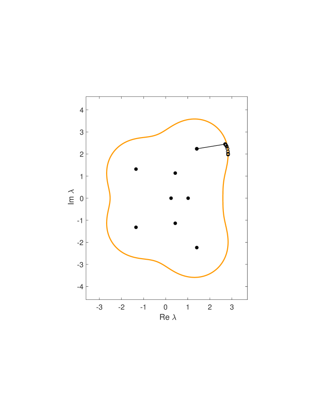
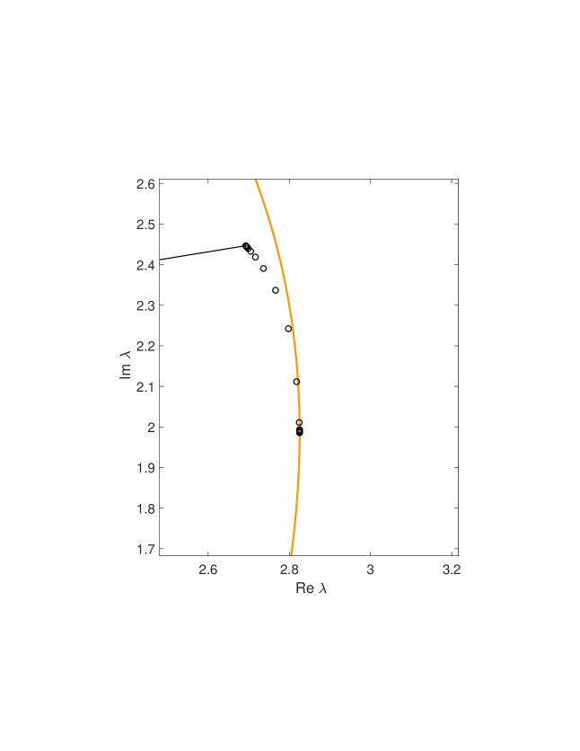
Fig. 3.1: Left: in black circles, iterates $\lambda_{k}$ of the splitting integrator (Algorithm 3.1) applied to the matrix $A$ of (3.19) with $f(\lambda,\overline{\lambda})={\mbox{\rm Re}}\,\lambda$ and $\varepsilon=1$. Right: zoom close to the stationary point.

Numerical example.

An illustration is given in Fig. 3.1 for $f(\lambda,\overline{\lambda})=-\frac{1}{2}(\lambda+\overline{\lambda})=-{\mbox{\rm Re}}\,\lambda$ and for the randomly chosen $8\times 8$ matrix

$$A=\left(\begin{array}[]{rrrrrrrr}0.91&1.17&-0.80&0.34&0.52&0&-1.39&-0.28\\ -0.05&0.54&1.91&1.68&1.67&1.38&1.62&2.50\\ 1.03&-1.35&-1.29&0.55&-1.37&-0.26&0.33&-0.89\\ -0.27&-1.05&-0.87&0.99&-1.23&0.04&-0.11&-0.62\\ -0.68&0.65&1.01&0.65&0.78&0.80&-0.18&-0.24\\ -0.16&-0.52&0.26&-0.61&-0.10&-0.04&0.22&0.37\\ -0.67&0.17&-0.69&2.23&-0.23&0.94&0.19&-0.22\\ -1.43&0.13&-0.89&0.06&1.26&0.28&0.05&0.03\end{array}\right).$$ (3.19)

The initial step size is set to $h=0.1$. The curve in the figure is the set, with $\varepsilon=1$ and the target eigenvalue $\lambda(M)$ the rightmost eigenvalue of a matrix $M$,

$$\{\lambda\left(A+\varepsilon E\right)\in\mathbb{C}\,:\;\text{$E\in\mathbb{C}^{n,n}$ with $\|E\|_{F}=1$}\}.$$

With our choice of $f(\lambda)=-{\mbox{\rm Re}}\,\lambda$ we aim to find a rightmost point of this set. (This set is the boundary of the $\varepsilon$-pseudospectrum of $A$. The problem of computing the real part of a rightmost point will be discussed in detail in Chapter III.)

II.4 Notes

The review article by Lewis and Overton (?) remains a basic reference on eigenvalue optimization, including a fascinating account of the history of the subject. There is, however, only a slight overlap of problems and techniques considered here and there.

The book by Absil, Mahony & Sepulchre (?) on optimization on matrix manifolds discusses alternative gradient-based methods to those considered here, though not specifically for eigenvalue optimization nor for low-rank matrix manifolds.

Rank-1 property of optimizers.

The rank-1 structure of optimizers in an eigenvalue optimization problem was first used by Guglielmi & Overton (?) who devised a rank-1 matrix iteration to compute the complex $\varepsilon$-pseudospectral abscissa and radius; see Section III.2 below.

The approach to eigenvalue optimization via a norm-constrained gradient flow and the associated rank-1 dynamics was first proposed and studied by Guglielmi & Lubich (?, ?), where it was used to compute the $\varepsilon$-pseudospectral abscissa and radius as well as sections of the boundary of the $\varepsilon$-pseudospectrum (see Chapter III). Our discussion of rank-1 dynamics in Section II.3.3 is based on Koch & Lubich (?).

Frobenius norm vs. matrix 2-norm.

In the approach described in this chapter (and further on in this work), perturbations are measured and constrained in the Frobenius norm. This choice is made because the Frobenius norm, other than the matrix 2-norm, is induced by an inner product, which simplifies many arguments. Not least, it allows us to work with gradient systems. However, the approach taken here with functional-reducing differential equations and their associated rank-1 dynamics is relevant also for the matrix 2-norm, because the optimizers with respect to the Frobenius norm are of rank 1, and so their Frobenius norm equals their 2-norm. Since the 2-norm of a matrix does not exceed its Frobenius norm, it follows that the rank-1 Frobenius-norm optimizers constrained by $\|\Delta\|_{F}\leq\varepsilon$ are simultaneously the 2-norm optimizers constrained by $\|\Delta\|_{2}\leq\varepsilon$.

Chapter III Pseudospectra

III.1 Complex $\varepsilon$-pseudospectrum

III.1.1 Motivation and definitions

As a motivating example for the $\varepsilon$-pseudospectrum of a matrix $A\in\mathbb{C}^{n,n}$, we consider the linear dynamical system $\dot{x}(t)=Ax(t)$. The system is asymptotically stable, i.e., solutions $x(t)$ converge to zero as $t\rightarrow\infty$ for all initial data, if and only if all eigenvalues of $A$ have negative real part. We now ask for the robustness of asymptotic stability under (complex unstructured) perturbations $\Delta\in\mathbb{C}^{n,n}$ of norm bounded by a given $\varepsilon>0$. This clearly depends on the choice of norm, and here we consider the Frobenius norm:

$$\|\cdot\|=\|\cdot\|_{F}.$$

For a normal matrix, the spectral decomposition yields that the perturbed system remains asymptotically stable for an arbitrary complex perturbation of norm at most $\varepsilon$ if for each eigenvalue $\lambda$ of $A$, the real part is bounded by ${\mbox{\rm Re}}\,\lambda+\varepsilon<0$. This condition is, however, not sufficient for non-normal matrices $A$.

The question posed is thus: Is the following real number negative?

$$\alpha_{\varepsilon}(A)=\max\{{\mbox{\rm Re}}\,\lambda:\ \ \Delta\in\mathbb{C}^{n,n} \|\Delta\|\leq\varepsilon$$ There exists with such that

$$\text{$\lambda$ is an eigenvalue of $A+\Delta$}\}.$$

This question is answered by solving a problem (II.1.1) with the function to be minimized given by $f(\lambda,\overline{\lambda})=-\tfrac{1}{2}(\lambda+\overline{\lambda})=-{\mbox{\rm Re}}\,\lambda$ (i.e., we maximize ${\mbox{\rm Re}}\,\lambda$).

It is useful to rephrase the question in terms of the $\varepsilon$-pseudospectrum, which is defined as follows; see also the notes in Section III.4.

• The complex $\varepsilon$-pseudospectrum of the matrix $A$ is the set

  $$\Lambda_{\varepsilon}(A)=\{\lambda\in\mathbb{C}:\ \ \text{$\lambda\in\Lambda(A+\Delta)$ for some $\Delta\in\mathbb{C}^{n,n}$ with $\|\Delta\|\leq\varepsilon$}\},$$ (1.1)

  where $\Lambda(M)\subset\mathbb{C}$ denotes the spectrum (i.e., set of eigenvalues) of a square matrix $M$.

The above quantity $\alpha_{\varepsilon}(A)$ can be rewritten more compactly as

$$\alpha_{\varepsilon}(A)=\max\{{\mbox{\rm Re}}\,\lambda:\ \lambda\in\Lambda_{\varepsilon}(A)\}.$$ (1.2)

It is known as the $\varepsilon$-pseudospectral abscissa of the matrix $A$.

An analogous quantity, of interest for discrete-time linear dynamical systems $x_{k+1}=Ax_{k}$, is the $\varepsilon$-pseudospectral radius of the matrix $A$,

$$\rho_{\varepsilon}(A)=\max\{|\lambda|:\ \lambda\in\Lambda_{\varepsilon}(A)\}.$$ (1.3)

III.1.2 Pseudospectrum, singular values, and resolvent bounds

The complex $\varepsilon$-pseudospectrum can be characterized in terms of singular values. The singular value decomposition of a matrix $M\in\mathbb{C}^{n,n}$ is $M=U\Sigma V^{*}$, with unitary matrices $U=(u_{1},\dots,u_{n})$ and $V=(v_{1},\dots,v_{n})$ formed by the left and right singular vectors $u_{k}$ and $v_{k}$, respectively, and with the real diagonal matrix $\Sigma={\rm diag}(\sigma_{1},\ldots,\sigma_{n})$ of the singular values $\sigma_{1}\geq\ldots\geq\sigma_{n}\geq 0$. We use the notation $\sigma_{k}(M)$ for the $k$th singular value of $M$ when we wish to indicate the dependence on $M$, and we write $\sigma_{\min}(M)=\sigma_{n}(M)$ for the smallest singular value.

• (Singular values and eigenvalues).  The complex $\varepsilon$-pseudospectrum of $A\in\mathbb{C}^{n,n}$ is characterized as

  $$\Lambda_{\varepsilon}(A) =\{\lambda\in\mathbb{C}:\ \sigma_{\min}(A-\lambda I)\leq\varepsilon\}$$ (1.4)

  $$=\{\lambda\in\mathbb{C}:\ \,\text{$\lambda\in\Lambda(A+\Delta)$\, for some $\Delta\in\mathbb{C}^{n,n}$ with $\|\Delta\|\leq\varepsilon$}\}.$$

  Moreover, the perturbation matrix $\Delta$ can be restricted to be of rank 1.

  • The result relies on the fact that the distance to singularity of a matrix $M$ equals its smallest singular value:

    $$\sigma_{\min}(M)=\min\{\|\Delta\|:\ \Delta\in\mathbb{C}^{n,n}\text{ is such that }M+\Delta\text{ is singular}\}.$$ (1.5)

    The perturbation of minimal norm is then the rank-1 matrix

    $$\Delta_{\star}=-\sigma_{n}u_{n}v_{n}^{*}$$ (1.6)

    (unique if $\sigma_{n}<\sigma_{n-1}$), where $\sigma_{n}=\sigma_{\min}(M)$ and $u_{n}$, $v_{n}$ are the left and right $n$th singular vectors. This perturbation is such that $M+\Delta_{\star}$ has the same singular value decomposition as $M$ except that the smallest singular value is replaced by zero.

    Choosing $M=A-\lambda I$ for $\lambda\in\mathbb{C}$ thus shows that $\sigma_{\min}(A-\lambda I)\leq\varepsilon$ if and only if there exists a matrix $\Delta\in\mathbb{C}^{n,n}$ of norm at most $\varepsilon$ such that $A-\lambda I+\Delta$ is singular, or equivalently, that $\lambda$ is an eigenvalue of $A+\Delta$.   $\sqcap$$\sqcup$

  Since $\sigma_{\min}(A-\lambda I)$ depends continuously on $\lambda$, Theorem III.1.2 implies that the boundary of the $\varepsilon$-pseudospectrum of $A$ is given as

  $$\partial\Lambda_{\varepsilon}(A)=\{\lambda\in\mathbb{C}:\ \sigma_{\min}(A-\lambda I)=\varepsilon\}.$$ (1.7)

• (Frobenius norm and matrix 2-norm).  Since for rank-1 matrices, the Frobenius norm and the matrix 2-norm are the same, Theorem III.1.2 and its proof show that the complex $\varepsilon$-pseudospectra defined with respect to these two norms are identical.

  Since $1/\sigma_{\min}(A-\lambda I)=\sigma_{\max}\bigl{(}(A-\lambda I)^{-1}\bigr{)}=\|(A-\lambda I)^{-1}\|_{2}$, we can reformulate (1.4) in terms of resolvents $(A-\lambda I)^{-1}$ as

  $$\Lambda_{\varepsilon}(A)=\{\lambda\in\mathbb{C}:\ \|(A-\lambda I)^{-1}\|_{2}\geq 1/\varepsilon\}.$$ (1.8)

  This allows us to characterize the $\varepsilon$-pseudospectral abscissa (1.2) as

  $$\alpha_{\varepsilon}(A)=\max\{{\mbox{\rm Re}}\,\lambda\,:\,\|(A-\lambda I)^{-1}\|_{2}\geq 1/\varepsilon\},$$

  which implies

  $$\frac{1}{\varepsilon}=\max_{\mathrm{Re}\,\lambda\geq\alpha_{\varepsilon}(A)}\|(A-\lambda I)^{-1}\|_{2}.$$ (1.9)

  If all eigenvalues of $A$ have negative real part, we define the stability radius (or distance to instability) as

  $$\varepsilon_{\star}>0\quad\text{such that}\quad\alpha_{\varepsilon_{\star}}(A)=0,$$

  i.e., there exists a perturbation $\Delta\in\mathbb{C}^{n,n}$ of Frobenius norm $\varepsilon_{\star}$ such that $A+\Delta$ has an eigenvalue on the imaginary axis, as opposed to all perturbations of smaller norm. The above formula then yields that the inverse stability radius $1/\varepsilon_{\star}$ is the smallest upper bound of the resolvent norm $\|(A-\lambda I)^{-1}\|_{2}$ for $\lambda$ in the right half-plane:

  $$\frac{1}{\varepsilon_{\star}}=\max_{\mathrm{Re}\,\lambda\geq 0}\|(A-\lambda I)^{-1}\|_{2}.$$ (1.10)

  As we discuss next, the $\varepsilon$-pseudospectral abscissa $\alpha_{\varepsilon}(A)$ and the stability radius $\varepsilon_{\star}$ are important quantities in bounding solutions of linear differential equations.

III.1.3 Transient bounds for linear differential equations

We describe two approaches to bounding solutions to linear differential equations, one for the matrix exponential ${\rm e}^{tA}$, which corresponds to the homogeneous initial value problem $\dot{x}(t)=Ax(t)$ with an arbitrary initial value $x(0)=x_{0}$, and the other approach for the inhomogeneous problem $\dot{x}(t)=Ax(t)+f(t)$ with zero initial value.

Bounds for the matrix exponential.

Via Theorem III.1.2, the transient behaviour of $\|{\rm e}^{tA}\|_{2}$ can be bounded in terms of the complex pseudospectrum. Here we illustrate this with a simple robust bound: Let $\Gamma_{\varepsilon}\subset\mathbb{C}$ be the boundary curve of a piecewise smooth domain (or several non-overlapping domains) whose closure covers $\Lambda_{\varepsilon}(A)$, and assume further that the real part of the rightmost point of $\Gamma_{\varepsilon}$ equals the pseudospectral abscissa $\alpha_{\varepsilon}(A)$. In particular, we may take $\Gamma_{\varepsilon}=\partial\Lambda_{\varepsilon}(A)$ when this is a piecewise regular curve. Using the Cauchy integral representation

$${\rm e}^{tA}=\frac{1}{2\pi\mathrm{i}}\int_{\Gamma_{\varepsilon}}{\rm e}^{t\lambda}\,(\lambda I-A)^{-1}\,d\lambda$$

and noting that by (1.8), $\|(\lambda I-A)^{-1}\|_{2}\leq 1/\varepsilon$ on $\Gamma_{\varepsilon}$, we find by taking norms that

$$\|{\rm e}^{tA}\|_{2}\leq\frac{\gamma_{\varepsilon}(t)}{\varepsilon}\quad\text{ with}\quad\gamma_{\varepsilon}(t)=\frac{1}{2\pi}\int_{\Gamma_{\varepsilon}}|{\rm e}^{t\lambda}|\,|d\lambda|\leq\frac{|\Gamma_{\varepsilon}|}{2\pi}\,{\rm e}^{t\alpha_{\varepsilon}(A)},$$ (1.11)

where $|\Gamma_{\varepsilon}|$ is the length of $\Gamma_{\varepsilon}$. This bound holds for every $\varepsilon>0$.

The same argument can be applied to a perturbed matrix $A+\Delta$ with $\Delta\in\mathbb{C}^{n,n}$ bounded by $\|\Delta\|_{2}\leq\delta<\varepsilon$. The Weyl inequality $\sigma_{i+j+1}(B+C)\leq\sigma_{i+1}(B)+\sigma_{j+1}(C)$ used with $i+1=n,\;j=0$ and $B=A-\lambda I+\Delta,\ C=-\Delta$ yields the lower bound

$$\sigma_{\min}(A+\Delta-\lambda I)\geq\sigma_{\min}(A-\lambda I)-\delta\geq\varepsilon-\delta\quad\text{for }\lambda\in\Gamma_{\varepsilon}.$$

We then obtain the robust transient bound

$$\|{\rm e}^{t(A+\Delta)}\|_{2}\leq\frac{\gamma_{\varepsilon}(t)}{\varepsilon-\delta}\qquad\text{for $\,\|\Delta\|_{2}\leq\delta\ $ and for all $\,\varepsilon>\delta$}.$$ (1.12)

This bound can be optimized over $\varepsilon>\delta$, provided that a bound for $|\Gamma_{\varepsilon}|$ and an algorithm for computing the pseudospectral abscissa $\alpha_{\varepsilon}(A)$ are available. Choosing $\varepsilon$ as the stability radius, $\varepsilon=\varepsilon_{\star}$, we have $\alpha_{\varepsilon_{\star}}(A)=0$, and so we obtain the time-uniform bound, for every $\delta<\varepsilon_{\star}$,

$$\|{\rm e}^{t(A+\Delta)}\|_{2}\leq\frac{|\Gamma_{\varepsilon_{\star}}|}{2\pi}\,\frac{1}{\varepsilon_{\star}-\delta}\quad\ t>0\ \Delta\in\mathbb{C}^{n,n} \,\|\Delta\|_{2}\leq\delta\$$ for all and for all with . (1.13)

Bounds for linear inhomogeneous differential equations.

We consider the differential equation $\dot{x}(t)=Ax(t)+f(t)$ with zero initial value for inhomogeneities $f\in L^{2}(0,\infty;\mathbb{C}^{n})$, where we assume that all eigenvalues of $A$ have negative real part. We extend $x(t)$ and $f(t)$ to $t<0$ by zero. Their Fourier transforms $\widehat{x}$ and $\widehat{f}$ are then related by $\mathrm{i}\omega\,\widehat{x}(\omega)=A\widehat{x}(\omega)+\widehat{f}(\omega)$ for all $\omega\in\mathbb{R}$, i.e.,

$$\widehat{x}(\omega)=(\mathrm{i}\omega I-A)^{-1}\widehat{f}(\omega),\qquad\omega\in\mathbb{R},$$

and hence the Plancherel formula yields

$$\int_{\mathbb{R}}\|x(t)\|^{2}\,dt=\int_{\mathbb{R}}\|\widehat{x}(\omega)\|^{2}\,d\omega=\int_{\mathbb{R}}\|(\mathrm{i}\omega I-A)^{-1}\widehat{f}(\omega)\|^{2}\,d\omega$$

$$\leq\max_{\omega\in\mathbb{R}}\|(\mathrm{i}\omega I-A)^{-1}\|_{2}^{2}\,\int_{\mathbb{R}}\|\widehat{f}(\omega)\|^{2}\,d\omega=\max_{\omega\in\mathbb{R}}\|(\mathrm{i}\omega I-A)^{-1}\|_{2}^{2}\,\int_{\mathbb{R}}\|f(t)\|^{2}\,dt.$$

Using (1.10) and the causality property that $x(t)$, for $0\leq t\leq T$, only depends on $f(\tau)$ with $0\leq\tau\leq t\leq T$ (which allows us to extend $f(t)$ by $0$ for $t>T$), we thus obtain the $L^{2}$ transient bound

$$\biggl{(}\int_{0}^{T}\|x(t)\|^{2}\,dt\biggr{)}^{1/2}\leq\frac{1}{\varepsilon_{\star}}\biggl{(}\int_{0}^{T}\|f(t)\|^{2}\,dt\biggr{)}^{1/2},\qquad 0\leq T\leq\infty,$$ (1.14)

where $\varepsilon_{\star}$ is the stability radius of $A$.

For perturbed differential equations $\dot{x}_{\Delta}(t)=(A+\Delta)x_{\Delta}(t)+f(t)$ with zero initial value with perturbation size $\|\Delta\|_{2}\leq\delta<\varepsilon_{\star}$ we obtain, by the same argument and using the Weyl inequality as before, the robust $L^{2}$ transient bound

$$\biggl{(}\int_{0}^{T}\|x_{\Delta}(t)\|^{2}\,dt\biggr{)}^{1/2}\leq\frac{1}{\varepsilon_{\star}-\delta}\biggl{(}\int_{0}^{T}\|f(t)\|^{2}\,dt\biggr{)}^{1/2},\qquad 0\leq T\leq\infty.$$ (1.15)

III.1.4 Extremal perturbations

The proof of Theorem III.1.2 also yields the following result on the perturbations $\Delta$ of minimal norm $\varepsilon$ such that $A+\Delta$ has a prescribed eigenvalue $\lambda$ on the boundary $\partial\Lambda_{\varepsilon}(A)$ of the complex $\varepsilon$-pseudospectrum of $A$.

• (Extremal complex perturbations).  Let $\lambda\in\partial\Lambda_{\varepsilon}(A)$, and let $\Delta\in\mathbb{C}^{n,n}$ of norm $\varepsilon$ be such that $A+\Delta$ has the eigenvalue $\lambda$. Then, $\Delta$ is of rank $1$.

  Assume now that $\varepsilon$ is a simple singular value of $A-\lambda I$ and that the corresponding left and right singular vectors are not orthogonal to each other. Then,

  $$\Delta=\varepsilon{\rm e}^{\mathrm{i}\theta}xy^{*},$$

  where ${\rm e}^{\mathrm{i}\theta}$ is the outer normal to $\partial\Lambda_{\varepsilon}(A)$ at $\lambda$, which is uniquely determined, and $x$ and $y$ are left and right eigenvectors of $A+\Delta$ to the eigenvalue $\lambda$, of unit norm and with $x^{*}y>0$.

  • By (1.7), we have $\sigma_{\min}(A-\lambda I)=\varepsilon$. The proof of Theorem III.1.2 then shows that $\Delta=-\varepsilon uv^{*},$ where $u$ and $v$ are left and right singular vectors of $A-\lambda I$, with

    $$(A-\lambda I+\Delta)v=0\quad\text{ and }\quad u^{*}(A-\lambda I+\Delta)=0,$$

    or equivalently, $(A+\Delta)v=\lambda v$ and $u^{*}(A+\Delta)=\lambda u^{*}$. This shows that $u$ and $v$ are left and right eigenvectors of $A+\Delta$.

    Assume now that $\varepsilon$ is a simple singular value of $A-\lambda I$ and that $u^{*}v\neq 0$. We show that $\partial\Lambda_{\varepsilon}(A)$ has the outer normal ${\rm e}^{\mathrm{i}\theta}$ at $\lambda$, where the angle $\theta$ is determined by

    $$u^{*}v=-\rho{\rm e}^{-\mathrm{i}\theta},\quad\rho>0.$$

    Let $\gamma(t)$, for $t$ near $0$, be a path in the complex plane with $\gamma(0)=\lambda\in\partial\Lambda_{\varepsilon}(A)$. With $\nu=\dot{\gamma}(0)$ we have, by the derivative formula of simple eigenvalues (see Theorem IX.IX.1),

    $$\frac{d}{dt}\bigg{|}_{t=0}\sigma_{\min}(A-\gamma(t)I) =\frac{\begin{pmatrix}u\\ v\end{pmatrix}^{*}\dfrac{d}{dt}\Big{|}_{t=0}\begin{pmatrix}0&A-\gamma(t)I\\ (A-\gamma(t)I)^{*}&0\end{pmatrix}\begin{pmatrix}u\\ v\end{pmatrix}}{\begin{pmatrix}u\\ v\end{pmatrix}^{*}\begin{pmatrix}u\\ v\end{pmatrix}}$$

    $$=-\tfrac{1}{2}\,{\mbox{\rm Re}}(\nu\,u^{*}v)=\tfrac{1}{2}\rho\,{\mbox{\rm Re}}(\nu{\rm e}^{-\mathrm{i}\theta}).$$

    This shows that $\nu={\rm e}^{\mathrm{i}\theta}$ is the unique direction of steepest ascent, which is orthogonal to the level set $\partial\Lambda_{\varepsilon}(A)$ and points out of $\Lambda_{\varepsilon}(A)$. Hence, ${\rm e}^{\mathrm{i}\theta}$ is the outer normal to $\partial\Lambda_{\varepsilon}(A)$ at $\lambda$.

    We set $x=-{\rm e}^{-\mathrm{i}\theta}u$ and $y=v$, which gives us a pair of left and right eigenvectors of $A+\Delta$ with $x^{*}y=\rho>0$. We then have

    $$\Delta=-\varepsilon uv^{*}=\varepsilon{\rm e}^{\mathrm{i}\theta}xy^{*},$$

    which proves the result.   $\sqcap$$\sqcup$

    As we will see, Theorems III.1.2 and III.1.4 motivate different approaches to computing the boundary of the $\varepsilon$-pseudospectrum (or just extremal points such as a rightmost point): methods that steer the smallest singular value of $A-\lambda I$ to $\varepsilon$, and methods that iterate on rank-1 matrices.

III.2 Computing the pseudospectral abscissa

As we have seen in the previous section, the $\varepsilon$-pseudospectral abscissa $\alpha_{\varepsilon}(A)$ is important for ensuring robust stability of a linear dynamical system. Various intriguing algorithms based on different ideas have been proposed to compute the pseudospectral abscissa:

• the criss-cross algorithm of Burke, Lewis & Overton (?), which is based on Theorem III.1.2 and on Byers’ Lemma given below;

• the rank-1 iteration of Guglielmi & Overton (?), which is based on Theorem III.1.4;

• the rank-1 constrained gradient flow algorithm of Guglielmi & Lubich (?); this is the approach presented in Chapter II for $f(\lambda,\overline{\lambda})=-\tfrac{1}{2}(\lambda+\overline{\lambda})=-{\mbox{\rm Re}}\,\lambda$;

• the subspace method of Kressner & Vandereycken (?).

III.2.1 Criss-cross algorithm

This remarkable algorithm was proposed and analysed by Burke, Lewis & Overton (?). It uses a sequence of vertical and horizontal searches in the complex plane to identify the intersection of a given line with $\partial\Lambda_{\varepsilon}(A)$. Horizontal searches yield updates to the approximation of $\alpha_{\varepsilon}(A)$ while vertical searches find favourable locations for the horizontal searches.

The criss-cross algorithm computes a monotonically growing sequence $(\alpha^{k})$ that converges to the complex $\varepsilon$-pseudospectral abscissa $\alpha_{\varepsilon}(A)$. In its basic form, it can be written as follows:

0. Initialize $\alpha^{0}=\max\{{\mbox{\rm Re}}\,\lambda\,:\,\lambda\in\Lambda(A)\}$.

1. For $k=0,1,2,\dots$ iterate

1.1 (Vertical search)

Find all real numbers $$\beta_{j} j 0 m$$, in increasing order for from to ,

such that $$\alpha^{k}+\mathrm{i}\beta_{j}\in\partial\Lambda_{\varepsilon}(A)$$. (2.1)

1.2 (Horizontal search) For $j=0,\dots,m-1$,

let the midpoint $$\beta_{j+1/2}=\tfrac{1}{2}(\beta_{j}+\beta_{j+1})$$;

if $$\alpha^{k}+\mathrm{i}\beta_{j+1/2}\in\Lambda_{\varepsilon}(A) \widehat{\alpha}_{j+1/2}$$, find the largest real number

such that $$\widehat{\alpha}_{j+1/2}+\mathrm{i}\beta_{j+1/2}\in\partial\Lambda_{\varepsilon}(A)$$ . (2.2)

1.3 Take $\alpha^{k+1}$ as the maximum of the $\widehat{\alpha}_{j+1/2}$.

To turn this into a viable algorithm, (2.1) and (2.2) need to be computed efficiently. This becomes possible thanks to the following basic lemma, applied to $A$ for (2.1) and to the rotated matrix $\mathrm{i}A$ for (2.2).

• (Byers’ Lemma).  Let $A\in\mathbb{C}^{n,n}$. For given real numbers $\alpha$ and $\beta$, the number $\varepsilon>0$ is a singular value of the matrix

  $$A-(\alpha+\mathrm{i}\beta){I}$$

  if and only if $\mathrm{i}\beta$ is an eigenvalue of the Hamiltonian matrix

  $$H(A,\alpha)=\left(\begin{array}[]{cc}-(A-\alpha I)^{*}&\varepsilon{I}\\ -\varepsilon{I}&A-\alpha{I}\end{array}\right).$$ (2.3)

  • After taking $A-\alpha{I}$ in the role of $A$, we can assume $\alpha=0$ in the following. The imaginary number $\mathrm{i}\beta$ is an eigenvalue of the Hamiltonian matrix (2.3) if and only if there exist nonzero vectors $u$ and $v$ such that

    $$\left(\begin{array}[]{cc}-A^{*}&\varepsilon{I}\\ {}-\varepsilon{I}&A\end{array}\right)\left(\begin{array}[]{c}u\\ v\end{array}\right)=\mathrm{i}\beta\left(\begin{array}[]{c}u\\ v\end{array}\right).$$ (2.4)

    This is equivalent to

    $$\left(A-\mathrm{i}\beta{I}\right)^{*}u=\varepsilon v,\qquad\left(A-\mathrm{i}\beta{I}\right)v=\varepsilon u,$$ (2.5)

    which expresses that $\varepsilon$ is a singular value of $A-\mathrm{i}\beta{I}$.   $\sqcap$$\sqcup$

    Using Lemma III.2.1, the vertical search (2.1) is done by computing all purely imaginary eigenvalues $\mathrm{i}\beta$ of the Hamiltonian matrix and discarding those eigenvalues among them for which $\varepsilon$ is not the smallest singular value of $A-(\alpha_{k}+\mathrm{i}\beta){I}$. The horizontal search (2.2) is done by computing the purely imaginary eigenvalue $\mathrm{i}\widehat{\alpha}_{j+1/2}$ of largest imaginary part of the Hamiltonian matrix that corresponds to the matrix $\mathrm{i}A$ in the role of $A$ and $-\beta_{j+1/2}$ in the role of $\alpha$. The method is written in pseudocode in Algorithm 2.2.

  The computational cost of an iteration step of the criss-cross algorithm is thus determined by computing imaginary eigenvalues of complex Hamiltonian $2n\times 2n$ matrices. All imaginary eigenvalues are needed in the vertical search and the ones of largest imaginary part in the horizontal search. In addition, the smallest singular values of complex $n\times n$ matrices need to be computed to decide if a given complex number is in $\Lambda_{\varepsilon}(A)$.

Data: Matrix $A$, $\varepsilon>0$, ${\rm tol}$ a given positive tolerance

Result: $\alpha_{\varepsilon}(A)$

begin

   1 Set $k=1$, $\alpha^{0}=\alpha(A)$

    while $\alpha^{k}-\alpha^{k-1}>{\rm tol}$ do

      2 Vertical iteration.

      43 Find all imaginary eigenvalues $\{\widehat{\beta}_{j}\}$ of $H(A,\alpha^{k})$ (see (2.3)) and collect those for which $\varepsilon$ is the smallest singular value of $A-(\alpha^{k}+\mathrm{i}\widehat{\beta}_{j})$ as $\{\beta_{j}\}_{j=0}^{m}$,

$$\beta_{0}\leq\beta_{1}\leq\beta_{2}\leq\ldots\leq\beta_{m-1}\leq\beta_{m}.$$

Horizontal iteration.

       for $j=0,\ldots,m-1$ do

         5 Compute the midpoints $\displaystyle{\beta_{j+1/2}=\frac{\beta_{j}+\beta_{j+1}}{2}}$

          Find the highest imaginary eigenvalue (i.e. with largest imaginary part) $\mathrm{i}\alpha_{j+1/2}$ of $H(\mathrm{i}A,\beta_{j+1/2})$ (see (2.3))

         

      6Set $k=k+1$

      7 Set $\alpha^{k+1}=\max\limits_{j=0,\ldots,m-1}\alpha_{j+1/2}$

      

   

Algorithm 2.2 Criss-cross algorithm

An illustration is given in Fig. 2.1 for the $8\times 8$ matrix in (II.3.19).

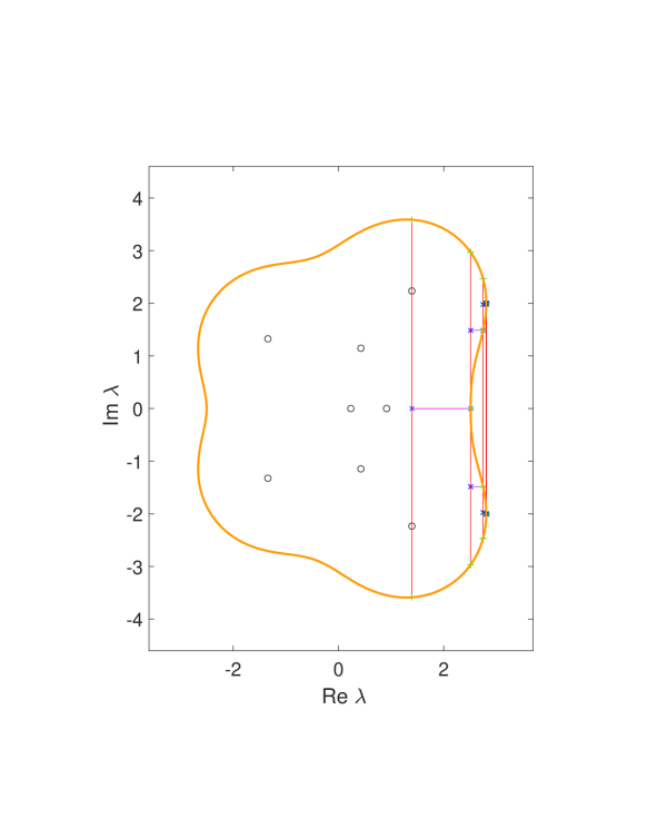
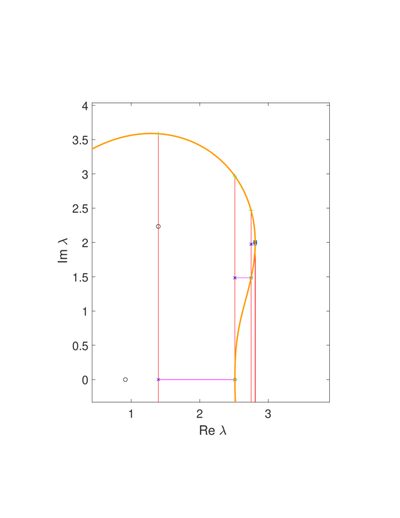
Fig. 2.1: Iterates of the criss cross algorithm for computing $\alpha_{\varepsilon}(A)$ for the matrix $A$ of (II.3.19) and $\varepsilon=1$. Right: zoom close to a rightmost point

Unconditional convergence.

As the following theorem by Burke, Lewis & Overton (?) shows, the sequence generated by the criss-cross algorithm always converges to the $\varepsilon$-pseudospectral abscissa.

• (Convergence of the criss-cross algorithm).  For every matrix $A\in\mathbb{C}^{n,n}$, the sequence $(\alpha^{k})$ of the criss-cross algorithm converges to the pseudospectral abscissa $\alpha_{\varepsilon}(A)$.

  • By construction, the sequence $(\alpha_{k})$ is a monotonically increasing sequence of real parts of points on $\partial\Lambda_{\varepsilon}(A)$, and it is bounded as $\Lambda_{\varepsilon}(A)$ is bounded. Therefore, $(\alpha_{k})$ converges to a limit $\alpha^{\star}$, which is the real part of some point on $\partial\Lambda_{\varepsilon}(A)$. Hence, $\alpha^{\star}\leq\alpha_{\varepsilon}(A)$. It remains to show that actually $\alpha^{\star}=\alpha_{\varepsilon}(A)$.

    To this end, we use the fact that every path-connected component of $\Lambda_{\varepsilon}(A)$ contains an eigenvalue of $A$. This is readily seen as follows: For any $\lambda_{1}\in\Lambda_{\varepsilon}(A)$, there exists a matrix $\Delta\in\mathbb{C}^{n,n}$ of norm at most $\varepsilon$ such that $\lambda_{1}$ is an eigenvalue of $A+\Delta$. Consider now the path $A+\theta\Delta$, $0\leq\theta\leq 1$. By the continuity of eigenvalues, to this path corresponds a path of eigenvalues $\lambda(\theta)$ of $A+\theta\Delta$ with $\lambda(1)=\lambda_{1}$, which connects $\lambda_{1}$ with the eigenvalue $\lambda(0)$ of $A$.

    Suppose $\alpha^{\star}<\alpha_{\varepsilon}(A)$. We lead this to a contradiction. Let $\lambda_{1}\in\Lambda_{\varepsilon}(A)$ be such that ${\mbox{\rm Re}}\,\lambda_{1}=\alpha_{\varepsilon}(A)$. Then there is a path $\lambda(\theta)$ to an eigenvalue $\lambda_{0}$ of $A$, which by construction has a real part that does not exceed $\alpha^{0}$ and hence is smaller than $\alpha^{\star}$. So there exist $0<\theta^{\star}<1$ such that $\lambda(\theta^{\star})\in\Lambda_{\theta^{\star}\!\varepsilon}(A)$ has real part $\alpha^{\star}$, so that $\lambda(\theta^{\star})=\alpha^{\star}+\mathrm{i}\beta^{\star}$ for some real $\beta^{\star}$. There exists a smallest interval $[\beta_{0},\beta_{1}]$ that contains $\beta^{\star}$ and has boundary points such that $\alpha^{\star}+\mathrm{i}\beta_{0},\alpha^{\star}+\mathrm{i}\beta_{1}\in\partial\Lambda_{\varepsilon}(A)$. Then, the points $\alpha^{\star}+\mathrm{i}\beta$ with $\beta_{0}<\beta<\beta_{1}$ are in the interior of $\Lambda_{\varepsilon}(A)$, and in particular this holds true for the midpoint $\beta=\tfrac{1}{2}(\beta_{0}+\beta_{1})$. Hence there exists an $\alpha>\alpha^{\star}$ such that $\alpha+\mathrm{i}\beta\in\partial\Lambda_{\varepsilon}(A)$. But then, also the criss-cross algorithm would have found an $\alpha^{k}>\alpha^{\star}$, in contradiction to the maximality of $\alpha^{\star}$. So we must have $\alpha^{\star}=\alpha_{\varepsilon}(A)$.   $\sqcap$$\sqcup$

Locally quadratic convergence.

We here show that the criss-cross algorithm converges locally quadratically under the following regularity assumption:

At every right-most point of the $$\varepsilon A$$-pseudospectrum of , the (2.6)

boundary curve $$\partial\Lambda_{\varepsilon}(A)$$ is smooth with nonzero curvature.

This condition is stronger than the condition of a simple smallest singular value of $A-\lambda I$ at right-most points $\lambda\in\Lambda_{\varepsilon}(A)$ imposed by Burke, Lewis & Overton (?), but it allows for a short proof of locally quadratic convergence.

• (Locally quadratic convergence of the criss-cross algorithm).  Under condition (2.6), the sequence $(\alpha^{k})$ of the criss-cross algorithm converges locally quadratically to $\alpha^{\star}=\alpha_{\varepsilon}(A)$ :

  $$0\leq\alpha^{\star}-\alpha^{k+1}\leq C(\alpha^{\star}-\alpha^{k})^{2},$$

  where $C$ is independent of $k$, provided that $\alpha^{k}$ is sufficiently close to $\alpha^{\star}$.

  • Near a right-most boundary point $\alpha^{\star}+\mathrm{i}\beta^{\star}$ of $\Lambda_{\varepsilon}(A)$, boundary points $\alpha+\mathrm{i}\beta$ are related by

    $$\alpha^{\star}-\alpha=f(\beta)=c^{2}(\beta^{\star}-\beta)^{2}+O((\beta^{\star}-\beta)^{3}),$$

    where $c\neq 0$ by condition (2.6). For the variables $\eta=\alpha^{\star}-\alpha$ and $\xi=c(\beta^{\star}-\beta)$ this relation becomes

    $$\eta=\varphi(\xi)=\xi^{2}+O(\xi^{3}).$$

    For a small $\delta>0$, let now $\xi_{+}=\delta$ and choose $\xi_{-}=-\delta+O(\delta^{2})$ such that $\varphi(\xi_{-})=\varphi(\xi_{+})=\delta^{2}(1+O(\delta))$. Then,

    $$\tfrac{1}{2}(\xi_{+}+\xi_{-})=O(\delta^{2})\quad\text{ and hence }\quad\varphi\bigl{(}\tfrac{1}{2}(\xi_{+}+\xi_{-})\bigr{)}=O(\delta^{4}),$$

    which yields

    $$\varphi\bigl{(}\tfrac{1}{2}(\xi_{+}+\xi_{-})\bigr{)}\leq C\varphi(\xi_{+})^{2}.$$

    Translated back to the original variables, this yields the stated result.   $\sqcap$$\sqcup$

III.2.2 Iteration on rank-1 matrices

Guglielmi and Overton (?) proposed a strikingly simple iterative algorithm for computing the pseudospectral abscissa that uses a sequence of rank-1 perturbations of the matrix. Working with rank-1 perturbations appears natural in view of Theorem III.1.4. Moreover, this lemma (with $\theta=0$) shows that at a point $\lambda\in\partial\Lambda_{\varepsilon}(A)$ such that ${\mbox{\rm Re}}\lambda=\alpha_{\varepsilon}(A)$, where the outer normal is horizontal to the right, the corresponding matrix perturbation $\Delta$ of norm $\varepsilon$ is such that $\Delta=\varepsilon xy^{*}$, where $x$ and $y$ are left and right eigenvectors, of unit norm and with $xy^{*}>0$, to the eigenvalue $\lambda$ of $A+\Delta$. This motivates the following fixed-point iteration.

Basic rank-1 iteration.

The basic iteration starts from two vectors $u_{0}$ and $v_{0}$ of unit norm and runs as follows for $k=0,1,2,\dots$:

Given a rank-$1$ matrix $E_{k}=u_{k}v_{k}^{*}$ of unit norm, compute the rightmost eigenvalue $\lambda_{k}$ of $A+\varepsilon E_{k}$ and left and right eigenvectors $x_{k}$ and $y_{k}$, of unit norm and with $x_{k}^{*}y_{k}>0$, and set $E_{k+1}=u_{k+1}v_{k+1}^{*}:=x_{k}y_{k}^{*}$.

Algorithm 2.3 gives a formal description. This algorithm requires in each step one computation of rightmost eigenvalues and associated eigenvectors of rank-$1$ perturbations to the matrix $A$, which can be computed at relatively small computational cost for large sparse matrices $A$, either combining the Cayley transformation approach of Meerbergen, Spence & Roose (?,?) with the Sherman-Morrison formula or by using an implicitly restarted Arnoldi method as implemented in ARPACK (Lehoucq, Sorensen & Yang, ?) and used in the MATLAB function eigs.

Data: Matrix $A$, $\varepsilon>0$, ${\rm tol}$ a given positive tolerance

Result: $r\leq\alpha_{\varepsilon}(A)$, $x,y$

begin

   1 Compute $x_{0}$ and $y_{0}$ left and right eigenvectors to the rightmost eigenvalue of $A$, both normalized to unit norm and with $x_{0}^{*}y_{0}>0$.

   2 Let $r_{-1}=-\infty$

   3 Compute $x_{0},y_{0}$, left and right eigenvectors to the rightmost eigenvalue $\lambda_{0}$ of $A$, with $x_{0},y_{0}$ of unit norm such that $x_{0}^{*}y_{0}>0$

   4 Set $r_{0}={\mbox{\rm Re}}(\lambda_{0})$

   5 Set $k=0$

    while $r_{k}-r_{k-1}>{\rm tol}$ do

      6 Compute $x_{k+1},y_{k+1}$, left and right eigenvectors to the rightmost eigenvalue $\lambda_{k+1}$ of $A+\varepsilon E_{k}$, $E_{k}=x_{k}y_{k}^{*}$, with $x_{k},y_{k}$ of unit norm such that $x_{k}^{*}y_{k}>0$

      7 Set $k=k+1$

      8 Set $r_{k}={\mbox{\rm Re}}(\lambda_{k})$

      

   9Set $r=r_{k}$

   10 Set $x=x_{k},y=y_{k}$

   

Algorithm 2.3 Rank-1 iteration

An illustration is given in Fig. 2.2 for the $8\times 8$ matrix (II.3.19).

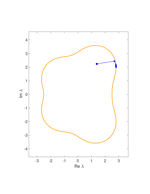
Fig. 2.2: Iterates $\lambda_{k}$ of the rank-1 iteration (Algorithm 2.3) applied to the matrix $A$ of (II.3.19) and $\varepsilon=1$.

The expectation is that ${\mbox{\rm Re}}\,\lambda_{k}$ converges to the $\varepsilon$-pseudospecral abscissa $\alpha_{\varepsilon}(A)$, as is observed in numerical experiments. Indeed, if the iteration converges, $\lambda_{k}\to\lambda$ and $x_{k}\to x$, $y_{k}\to y$, then $x,y$ are of unit norm with $x^{*}y>0$ and

$$x,y \lambda A+\varepsilon xy^{*}$$ are left and right eigenvectors to the rightmost eigenvalue of . (2.7)

This implies $(A-\lambda I)y=-\varepsilon x$ and $x^{*}(A-\lambda I)=-\varepsilon y^{*}$, which shows that $A-\lambda I$ has the singular value $\varepsilon$ (as is required for having $\lambda\in\partial\Lambda_{\varepsilon}(A)$ by (1.7)) — though $\varepsilon$ is here not known to be the smallest singular value. Furthermore, the gradient of the associated singular value is $x^{*}y>0$, that is, the gradient is horizontal to the right in the complex plane. By Theorem III.1.4, this implies that $\lambda\in\partial\Lambda_{\varepsilon}(A)$ with outer normal 1 if $\varepsilon$ is indeed the smallest singular value of $A-\lambda I$.

Moreover, in the interpretation of Theorem II.II.2.3 and Remark II.II.2.3, the property (2.7) implies that $E=xy^{*}$ is a stationary point (though not necessarily a maximum) of the eigenvalue optimization problem to find

$$\arg\max_{\|E\|_{F}\leq 1}{\mbox{\rm Re}}\,\lambda(A+\varepsilon E),$$ (2.8)

i.e. Problem (II.1.1) with $f(\lambda,\overline{\lambda})=-{\mbox{\rm Re}}\,\lambda$.

There exist no results about global convergence of the rank-1 iteration. Local linear convergence can be shown for a sufficiently small ratio of the two smallest singular values, $\varepsilon/\sigma_{n-1}(A-\lambda I)$, by studying the derivative of the iteration map at a stationary point. This requires bounds of derivatives of eigenvectors using appropriate representations of the group inverse, as laid out in the Appendix.

Monotone rank-1 iteration.

The simple rank-1 iteration described above is not guaranteed to yield a monotonically increasing sequence $({\mbox{\rm Re}}\,\lambda_{k})$. Guglielmi and Overton (?) also proposed a monotone variant that is described in the following.

For given vectors $u,v$ of unit norm, we start from the rank-1 perturbation $A+\varepsilon uv^{*}$ with rightmost eigenvalue $\lambda_{0}$, assumed to be simple. Let $x,y$ be left and right eigenvectors associated with $\lambda_{0}$, of unit norm and with $x^{*}y>0$. We still have a further degree of freedom in scaling $x$ and $y$, i.e. choosing the argument of the complex numbers $\alpha=u^{*}x$ and $\beta=v^{*}y$ of fixed modulus.

— If $|\alpha|\geq|\beta|$, then we scale $x$ such that $\alpha$ is real and positive. Since we require $x^{*}y>0$, this also determines $y$ uniquely.

— If $|\alpha|<|\beta|$, then we scale $y$ such that $\beta$ is real and positive. Since we require $x^{*}y>0$, this also determines $x$ uniquely.

With this particular scaling, we consider, for $0\leq t\leq 1$, a family of matrices

$$B(t)=A+\varepsilon p(t)q(t)^{*},\qquad 0\leq t\leq 1,$$ (2.9)

that interpolates between $A+\varepsilon uv^{*}$ at $t=0$ and $A+\varepsilon xy^{*}$ at $t=1$:

$$p(t)=\frac{tx+(1-t)u}{\|tx+(1-t)u\|},\quad q(t)=\frac{ty+(1-t)v}{\|ty+(1-t)v\|}.$$ (2.10)

The following lemma will allow us to formulate a rank-1 iteration with monotonically increasing ${\mbox{\rm Re}}\,\lambda_{k}$.

• (Monotonicity near $t=0$).  Let $B(t)$, $0\leq t\leq 1$, be defined as above with the stated scaling of the eigenvectors. Let $\lambda(t)$, $0\leq t\leq 1$, be the continuous path of eigenvalues of $B(t)$ with $\lambda(0)=\lambda_{0}$. If $\lambda_{0}$ is a simple eigenvalue of $A+\varepsilon uv^{*}$, then $\lambda(t)$ is differentiable at $0$ and

  $${\mbox{\rm Re}}\,\dot{\lambda}(0)\geq 0.$$

  The inequality is strict except in the following two cases:

  1. $\alpha=\beta=1$;

  2. $\alpha$ and $\beta$ are both real, of equal modulus and opposite sign.

  • By Theorem IX.IX.1 we have, with $\kappa=1/(x^{*}y)>0$,

    $$\dot{\lambda}(0)=\frac{x^{*}\dot{B}(t)y}{x^{*}y}=\varepsilon\kappa\Bigl{(}x^{*}\bigl{(}\dot{p}(0)q(0)^{*}+p(0)\dot{q}(0)^{*}\bigr{)}y\Bigr{)}.$$

    We find $p(0)=u$, $q(0)=v$ and

    $$\dot{p}(0)=(x-u)-u{\mbox{\rm Re}}(u^{*}(x-u))=x-u{\mbox{\rm Re}}(u^{*}x)=x-u{\mbox{\rm Re}}\,\alpha,\quad\dot{q}(0)=y-v{\mbox{\rm Re}}\,\beta$$

    This yields

    $${\mbox{\rm Re}}\,\dot{\lambda}(0) =\varepsilon\kappa{\mbox{\rm Re}}\Bigl{(}x^{*}(x-u{\mbox{\rm Re}}\,\alpha)v^{*}y+x^{*}u(y-v{\mbox{\rm Re}}\,\beta)^{*}y\Bigr{)}$$

    $$=\varepsilon\kappa\bigl{(}{\mbox{\rm Re}}\,\beta-{\mbox{\rm Re}}\,\alpha\,{\mbox{\rm Re}}(\overline{\alpha}\beta)+{\mbox{\rm Re}}\,\alpha-{\mbox{\rm Re}},\beta\,{\mbox{\rm Re}}(\overline{\alpha}\beta)\bigr{)},$$

    that is,

    $${\mbox{\rm Re}}\,\dot{\lambda}(0)=\varepsilon\kappa\left(1-{\mbox{\rm Re}}(\overline{\alpha}\beta)\right)\left({\mbox{\rm Re}}\,\alpha+{\mbox{\rm Re}}\,\beta\right).$$ (2.11)

    With our scaling, the right-hand side is positive except in Case 1. oder 2., where it vanishes.   $\sqcap$$\sqcup$

Lemma III.2.2 guarantees that ${\mbox{\rm Re}}~\lambda(t)>{\mbox{\rm Re}}~\lambda(0)$ for sufficiently small $t$. Hence the idea is to perform zero or more times the computation of the rightmost eigenvalue $\lambda(t)$ of (2.9)-(2.10) until

$${\mbox{\rm Re}}~\lambda(t)>{\mbox{\rm Re}}~\lambda(0)+\frac{t}{2}\,{\mbox{\rm Re}}~\dot{\lambda}(0)$$

with ${\mbox{\rm Re}}~\dot{\lambda}(0)$ given by (2.11), replacing $t$ by $t/2$ until the inequality is fulfilled.

In the $k$th iteration step, starting from $(u,v)=(u_{k},v_{k})$ and $\lambda(0)=\lambda_{k}$, we determine in this way $t>0$ such that ${\mbox{\rm Re}}~\lambda(t)$ satisfies the above condition and then set $\lambda_{k+1}=\lambda(t)$ and $(u_{k+1},v_{k+1})=(p(t),q(t))$. The sequence of the real parts of the eigenvalues ${\mbox{\rm Re}}\,\lambda_{k}$ is then monotonically increasing. In more detail, the variant is formulated in Algorithm 2.4.

Data: Matrix $A$, $\varepsilon>0$, ${\rm tol}$ a given positive tolerance

Result: $r\leq\alpha_{\varepsilon}(A)$, $x,y$

begin

   1 Compute $x_{0}$ and $y_{0}$ left and right eigenvectors to the rightmost eigenvalue of $A$, both normalized to unit norm and with $x_{0}^{*}y_{0}>0$.

   2 Let $r_{-1}=-\infty$

   3 Compute $x_{0},y_{0}$, left and right eigenvectors to the rightmost eigenvalue $\lambda_{0}$ of $A$, with $x_{0},y_{0}$ of unit norm such that $x_{0}^{*}y_{0}>0$

   4 Set $r_{0}={\mbox{\rm Re}}(\lambda_{0})$

   5 Set $k=0$

    while $r_{k}-r_{k-1}>{\rm tol}$ do

      6 Compute $x_{k+1},y_{k+1}$, left and right eigenvectors to the rightmost eigenvalue $\lambda_{k+1}$ of $A+\varepsilon E_{k}$, $E_{k}=x_{k}y_{k}^{*}$, with $x_{k},y_{k}$ of unit norm such that $x_{k}^{*}y_{k}>0$

      7 Set $\lambda=\lambda_{k+1}$

      8 Set $t=1$

       repeat

         9 Set $t=t/2$

         10 Compute $x(t),y(t)$ according to (2.10)

         11 Compute $\lambda(t)$

         

      until ${\mbox{\rm Re}}\lambda>{\mbox{\rm Re}}\lambda_{k}$

      12Set $x_{k+1}=x(t)$, $y_{k+1}=y(t)$

      13 Set $k=k+1$

      14 Set $r_{k}={\mbox{\rm Re}}(\lambda_{k})$

      

   15Set $r=r_{k}$, $x=x_{k},y=y_{k}$

   16 Halt

   

Algorithm 2.4 Rank-1 iteration: monotone version

• (Convergence of the monotone rank-1 iteration).  If the iteration sequence stays away from Case 2 in Lemma III.2.2, then the monotone rank-1 iteration converges to a stationary point of the eigenvalue optimization problem (2.8), i.e., the limits

  $$\lambda=\lim_{k\to\infty}\lambda_{k},\quad u=\lim_{k\to\infty}u_{k},\quad v=\lim_{k\to\infty}v_{k}$$

  exist, and the stationarity condition (2.7) is satisfied. In particular, $\varepsilon$ is a singular value of $A-\lambda I$ with left and right singular vectors $u$ and $v$. If $\varepsilon$ is the smallest singular value, then $\lambda\in\partial\Lambda_{\varepsilon}(A)$ with horizontal rightward outer normal.

  We note that near a stationary point (2.7), where $\alpha=\beta=1$, Case 2 in Lemma III.2.2 cannot occur.

  • Since the sequence $({\mbox{\rm Re}}\,\lambda_{k})$ is monotonically increasing and bounded, it converges. This implies that in the limit, both sides of (2.11) are zero, and hence one of the two cases 1 or 2 in Lemma III.2.2 must avail in the limit. By assumption, we have excluded the exceptional Case 2. In the remaining Case 1, $\alpha=\beta=1$ in the limit, i.e. $u=x$ and $v=y$ in the limit, and hence the iteration converges and the stationarity condition (2.7) is fulfilled. As noted before, this implies the further statements.   $\sqcap$$\sqcup$

  Figure 2.3 shows the $\varepsilon$-pseudospectrum of the matrix $A$ in (3.19) for $\varepsilon=1$ as well as the $\varepsilon$-level set of $\sigma_{n-1}(A-zI)$ and $\sigma_{n-2}(A-zI)$ (the inner curves).

The points to which the algorithms may converge are given by the $5$ points indicated by bullets. The locally rightmost ones are locally attractive while the other ones turn out to be locally unstable.

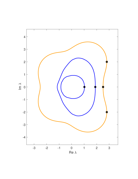
Fig. 2.3: The outer curve is the boundary of the pseudospectrum $\Lambda_{\varepsilon}(A)$ and the inner curves are the $\varepsilon$-level sets of $\sigma_{n-1}(A-zI)$ and $\sigma_{n-2}(A-zI)$ for the matrix $A$ of (II.3.19) and $\varepsilon=1$. The black points are fixed points of the algorithm by Guglielmi & Overton, as well as stationary points of the differential equations (II.3.8) and (II.3.9).

III.2.3 Discretized rank-1 matrix differential equation

A different iteration on rank-1 matrices results from the rank-1 projected gradient system of Section II.3.3 for the minimization function $f(\lambda,\overline{\lambda})=-\tfrac{1}{2}(\lambda+\overline{\lambda})=-{\mbox{\rm Re}}\,\lambda$ after discretization as in Section II.3.4 (see Algorithm II.3.1), as was first proposed similarly by Guglielmi & Lubich (?), though with a different time stepping method. The so obtained rank-1 iteration yields a sequence of rank-1 matrices $E_{k}=u_{k}v_{k}^{*}$ of unit norm and a sequence of eigenvalues $\lambda_{k}\in\Lambda_{\varepsilon}(A)$ of $A+\varepsilon E_{k}$ with monotonically growing real part, which converges to a stationary point (2.7); see Theorems II.II.3.3 and Remark II.II.3.3, and also Lemma II.II.3.4 for the splitting method. The computational cost per step is essentially the same as in the rank-1 iterations of the previous subsection. A numerical example was already presented in Section II.3.4.

Conceptually, the approach of first deriving a suitable differential equation and then using an adaptive time-stepping to arrive at a stationary point is different from directly devising an iteration. Different tools are available and made use of in the two approaches. For example, the tangent space of the manifold of rank-1 matrices is a natural concept in the time-continuous setting though not so in the time-discrete setting. This enhanced toolbox results in efficient algorithms that would not be obtained from a purely discrete viewpoint.

III.2.4 Acceleration by a subspace method

Kressner and Vandereycken (?) proposed a subspace method to accelerate the basic rank-1 iteration described in Subsection III.2.2. For the subspace expansion, they essentially do a step of Algorithm 2.3 and add the obtained eigenvector to the subspace. Along the way they compute orthonormal bases $V_{k}\in\mathbb{C}^{n\times k}$ of nested subspaces. A key element is the computation of the rightmost point of the $\varepsilon$-pseudospectrum of the rectangular matrix pencil $AV_{k}-\lambda V_{k}$ in place of $A-\lambda I$,

$$\Lambda_{\varepsilon}(AV_{k},V_{k})=\{\lambda\in\mathbb{C}\,:\,\sigma_{\min}(AV_{k}-\lambda V_{k})=\varepsilon\}.$$

These pseudospectra are nested: $\Lambda_{\varepsilon}(AV_{k},V_{k})\subset\Lambda_{\varepsilon}(AV_{k+1},V_{k+1})\subset\Lambda_{\varepsilon}(A)$. The rightmost point of $\Lambda_{\varepsilon}(AV_{k},V_{k})$ is computed by a variant of the criss-cross algorithm. The basic algorithm is given in Algorithm 2.5.

Data: Matrix $A$, $\varepsilon>0$

Result: Approximation $\mu_{\alpha}$ to a locally rightmost point of $\Lambda_{\varepsilon}(A)$.

begin

   1 Compute the rightmost eigenvalue $\lambda_{0}$ and normalized right eigenvector $y_{0}$ of $A$.

   2 Set $\widehat{V}_{1}=y_{0}$.

   3 for $k=1,2,\dots$ until converged do

      4 Compute the rightmost point $\mu_{k}$ of $\Lambda_{\varepsilon}(AV_{k},V_{k})$.

      5 Compute left/right singular vectors $u_{k}$ and $v_{k}$ to $\sigma_{\min}(A-\mu_{k}I)$. Set $E_{k}=-u_{k}v_{k}^{*}$.

      6 Compute the rightmost eigenvalue $\lambda_{k}$ and right eigenvector $y_{k}$ of $A+\varepsilon E_{k}$. Compute $V_{k+1}=\,$orth$([V_{k},y_{k}])$.

      

   7Set $\mu_{\alpha}=\mu_{k}$.

Algorithm 2.5 Subspace method.

Kressner and Vandereycken (?) show that the sequence $(\mu_{k})$ grows monotonically, as a consequence of the growth of the nested subspaces. A simplified version of the algorithm, where the right singular vector $v_{k}$ instead of the right eigenvector $y_{k}$ is added to the subspace, is shown to converge locally superlinearly to the pseudospectral abscissa.

III.3 Tracing the boundary of the pseudospectrum

In this section we describe two algorithms for boundary tracing. While there exist path-following methods to obtain pseudospectral contours (e.g. those implemented in Eigtool), the computation becomes expensive for large matrices. Here we use instead the low-rank structure of the extremal perturbations, which allows us to treat also large sparse matrices efficiently; see Section II.3.2.

We present two algorithms. The first algorithm, to which we refer as the tangential–transversal algorithm, makes use of a combination of the differential equation (II.3.8) and a similar differential equation that moves eigenvalues horizontally to the boundary. The second algorithm, which we call the ladder algorithm, aims to compute, for an iteratively constructed sequence of points outside the $\varepsilon$-pseudospectrum, the corresponding nearest points in the $\varepsilon$-pseudospectrum. Both algorithms require repeatedly the computation of the eigenvalue of a rank-1 perturbation to $A$ that is nearest to a given complex number. This can be done efficiently also for large matrices, using inverse power iteration combined with the Sherman-Morrison formula.

The ladder algorithm extends readily to real and structured pseudospectra, for which the few algorithms proposed in the literature (as implemented in Seigtool) are restricted to just a few structures and turn out to be extremely demanding from a computational point of view.

III.3.1 Tangential–transversal algorithm

The algorithm alternates between a time step for the system of differential equations (II.3.8) and the following system of differential equations for vectors $u(t)$ and $v(t)$ of unit norm. This second system is a simplified variant of (II.3.8) for $G=-xy^{*}$, where $x$ and $y$ are left and right eigenvectors, respectively, both of unit norm and with $x^{*}y>0$, of an eigenvalue $\lambda$ of the rank-1 perturbed matrix $A+\varepsilon uv^{*}$:

$$\begin{array}[]{rcl}\dot{u}&=&(I-uu^{*})xy^{*}v\\[2.84526pt] \dot{v}&=&(I-vv^{*})yx^{*}u.\end{array}$$ (3.1)

The system preserves the unit norm of $u$ and $v$, since $u^{*}\dot{u}=0$ and $v^{*}\dot{v}=0$. As we show in the next lemma, the system has the property that for a path of simple eigenvalues $\lambda(t)$ of $A+\varepsilon u(t)v(t)^{*}$, the derivative $\dot{\lambda}(t)$ is real and positive, continuing to a stationary point where $A-\lambda I$ has the singular value $\varepsilon$. By Theorem III.1.2 it therefore stops at the boundary $\partial\Lambda_{\varepsilon}(A)$ when $\varepsilon$ is the smallest singular value. While in theory, a trajectory might stop at an interior point where the singular value $\varepsilon$ is not the smallest one, this appears to be an unstable case that is not observed in computations.

• (Horizontal motion of an eigenvalue).  Along a path of simple eigenvalues $\lambda(t)$ of $A+\varepsilon u(t)v(t)^{*}$, where $u,v$ of unit norm solve (3.1), we have that

  $$\dot{\lambda}(t) t$$ is real and positive for all  .

  In the limit $\lambda_{\star}=\lim_{t\to\infty}\lambda(t)$, the matrix $A-\lambda_{\star}I$ has the singular value $\varepsilon$.

  • The perturbation theory of eigenvalues (see Theorem IX.IX.1) shows that

    $$\dot{\lambda}=\frac{x^{*}\frac{d}{dt}(A+\varepsilon uv^{*})\,y}{x^{*}y}=\varepsilon\,\frac{x^{*}\left({\dot{u}}v^{*}+u{\dot{v}}^{*}\right)y}{x^{*}y}.$$

    With $\alpha=u^{*}x$ and $\beta=v^{*}y$, we obtain

    $$\dot{\lambda}=\frac{\varepsilon}{x^{*}y}\Bigl{(}|\alpha|^{2}\cdot\|y-\beta v\|^{2}+|\beta|^{2}\cdot\|x-\alpha u\|^{2}\Bigr{)}\in\mathbb{R},\ \geq 0.$$

    In a stationary point of (3.1), $u$ and $x$ are collinear, and so are $v$ and $y$. It follows that $uv^{*}={\rm e}^{\mathrm{i}\theta}xy^{*}$ for some real $\theta$. We thus have

    $$(A+\varepsilon{\rm e}^{\mathrm{i}\theta}xy^{*})y=\lambda y,\qquad x^{*}(A+\varepsilon{\rm e}^{\mathrm{i}\theta}xy^{*})=\lambda x^{*},$$

    or equivalently

    $$(A-\lambda I)y=\varepsilon{\rm e}^{\mathrm{i}\theta}x,\qquad(A-\lambda I)^{*}{\rm e}^{\mathrm{i}\theta}x=\varepsilon y,$$

    which states that ${\rm e}^{\mathrm{i}\theta}x$ and $y$ are left and right singular vectors to the singular value $\varepsilon$ of $A-\lambda I$.   $\sqcap$$\sqcup$

    While (3.1) moves eigenvalues horizontally to the right, the differential equation (II.3.8) moves an eigenvalue on the boundary along a path that starts tangentially to the boundary, as is shown by the following lemma.

    • (Tangential motion of an eigenvalue from the boundary).  Let $\lambda_{0}\in\partial\Lambda_{\varepsilon}(A)$ be on a smooth section of the boundary, with outer normal ${\rm e}^{\mathrm{i}\theta}$ at $\lambda_{0}$ for $0<|\theta|\leq\pi/2$. Let $u_{0}$ and $v_{0}$ of unit norm be such that $A+\varepsilon u_{0}v_{0}^{*}$ has $\lambda_{0}$ as a simple eigenvalue. Let $u(t)$ and $v(t)$ be solutions of the system of differential equations (II.3.8) with $G=-xy^{*}$ with initial values $u_{0}$ and $v_{0}$. Then, the path of eigenvalues $\lambda(t)$ of $A+\varepsilon u(t)v(t)^{*}$ with $\lambda(0)=\lambda_{0}$ has $\dot{\lambda}(0)\neq 0$ and

      $$\dot{\lambda}(0) \partial\Lambda_{\varepsilon}(A) \lambda_{0}$$ is tangential to at .

      • By Theorem III.1.4, we have $u_{0}v_{0}^{*}={\rm e}^{\mathrm{i}\theta}x_{0}y_{0}^{*}.$ We then find, inserting (II.3.8) for $\dot{u}$ and $\dot{v}$,

        $$\dot{\lambda}(0) =\frac{x_{0}^{*}\,\frac{d}{dt}\big{|}_{t=0}(A+\varepsilon u(t)v(t)^{*})\,y_{0}}{x_{0}^{*}y_{0}}$$

        $$=\frac{\varepsilon}{x_{0}^{*}y_{0}}\,x_{0}^{*}\bigl{(}\dot{u}(0)v(0)^{*}+u(0)\dot{v}(0)^{*}\bigr{)}y_{0}$$

        $$=\frac{\varepsilon}{x_{0}^{*}y_{0}}\,\mathrm{i}\,{\mbox{\rm Im}}(u_{0}^{*}x_{0}y_{0}^{*}v_{0})x_{0}^{*}u_{0}v_{0}^{*}y_{0}$$

        $$=\frac{\varepsilon}{x_{0}^{*}y_{0}}\,\mathrm{i}\,{\mbox{\rm Im}}({\rm e}^{-\mathrm{i}\theta})\,{\rm e}^{\mathrm{i}\theta}.$$

        Since $x_{0}^{*}y_{0}>0$, we find that $\dot{\lambda}(0)$ points into the tangential direction $-\mathrm{i}\,{\rm e}^{\mathrm{i}\theta}\,\mathrm{sign}(\theta)$.   $\sqcap$$\sqcup$

Description of the algorithm.

Lemmas III.3.1 and III.3.1 motivate the following algorithm for tracing the boundary of the $\varepsilon$-pseudospectrum $\Lambda_{\varepsilon}(A)$. Suppose that $\lambda_{0}$ is a simple eigenvalue of $A+\varepsilon u_{0}v_{0}^{*}$ lying on a smooth section of the boundary $\partial\Lambda_{\varepsilon}(A)$, with a priori unknown outer normal ${\rm e}^{\mathrm{i}\theta_{0}}$. By Theorem III.1.4, $u_{0}v_{0}^{*}={\rm e}^{\mathrm{i}\theta_{0}}x_{0}y_{0}^{*}$, where $x_{0}$ and $y_{0}$ are left and right eigenvectors of $A+\varepsilon u_{0}v_{0}^{*}$, both of unit norm and with $x_{0}^{*}y_{0}>0$. This fact allows us to determine the outer normal as

$${\rm e}^{\mathrm{i}\theta_{0}}=\frac{|u_{0}^{*}v_{0}|}{u_{0}^{*}v_{0}}.$$ (3.2)

We first consider the tangential differential equation (II.3.8) with $G=-xy^{*}$ for the rotated matrix $\mathrm{i}{\rm e}^{-\mathrm{i}\theta_{0}}A$, which leads us to the case $\theta=\pi/2$ in Lemma III.3.1. We make a time step of stepsize $h$ with the splitting method presented in Chapter II, followed by normalization of $u$ and $v$; at $t_{1}=t_{0}+h$ this yields a rank-1 matrix $\widetilde{E}_{1}=\tilde{u}_{1}\tilde{v}_{1}^{*}$ of unit norm. (Note that this step does not require to actually compute the rotated matrix.) Since $\dot{\lambda}(t_{0})$ is tangential to the boundary $\partial\Lambda_{\varepsilon}(A)$ at $\lambda_{0}$, the eigenvalue $\tilde{\lambda}_{1}$ of $A+\varepsilon\widetilde{E}_{1}$ lies in $\Lambda_{\varepsilon}(A)$ and is $O(h^{2})$ close to the boundary.

With initial values $\tilde{u}_{1},\tilde{v}_{1}$ we then consider the differential equation (3.1) for the rotated matrix ${\rm e}^{-\mathrm{i}\theta_{0}}A$ in order to reach the boundary with a horizontal trajectory. We integrate (3.1) until we stop at a stationary point $E_{1}=u_{1}v_{1}^{*}$. There, a singular value of $A-\lambda I$ equals $\varepsilon$ (by Lemma III.3.1), which takes us to the boundary $\partial\Lambda_{\varepsilon}(A)$ provided we start sufficiently close to it.

We then continue the above alternating integration from $\lambda_{1}\in\partial\Lambda_{\varepsilon}(A)$ and the associated vectors $u_{1},v_{1}$.

The algorithm as described computes a part of $\partial\Lambda_{\varepsilon}(A)$ to the right of $\lambda_{0}$. To go to the left, we change the direction of time in the tangential differential equation (II.3.8), i.e., we take a negative stepsize $h$. The algorithm is summarized in Algorithm 3.6.

Data: Matrix $A$, initial vectors $u,v$ of unit norm such that the eigenvalue $\lambda$ of $A+\varepsilon uv^{*}$ lies on $\partial\Lambda_{\varepsilon}(A)$, stepsize $h$, number $N$ of desired boundary points, ${\rm tol}$ a given positive tolerance

Result: vector $\Gamma$ of $N$ consecutive boundary points

begin

    for i=1,…,N do

      1 Set $\zeta=u^{*}v/|u^{*}v|$

      2 Compute the approximate solution $\widetilde{u}_{1},\widetilde{v}_{1}$ of (II.3.8) for the rotated matrix $\mathrm{i}\zeta A$ with initial data $\mathrm{i}\zeta u,v$ doing a single normalized Euler step of size $h$

      3 Let $u_{0}=-\mathrm{i}\widetilde{u}_{1}$, $v_{0}=\widetilde{v}_{1}$

       for $k=1,2,\ldots$ until convergence do

         4 Compute the approximate solution $u_{k},v_{k}$ of (3.1) for the rotated matrix $\zeta A$ with adaptive stepsize $h_{k}$ (as in Chapter II)

         5 Compute the rightmost eigenvalue $\lambda_{k}$ of $\zeta A+\varepsilon u_{k}\,v_{k}^{*}$

         

      6Set $u=u_{k}/\zeta$, $v=v_{k}$

      7 Store $\lambda_{k}/\zeta$ into $\Gamma$

      

   

Algorithm 3.6 tangential–transversal algorithm for tracing the boundary of the $\varepsilon$-pseudospectrum

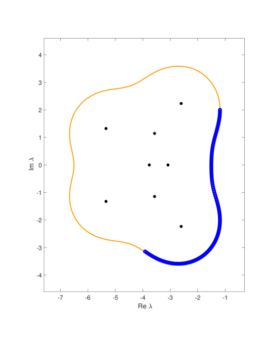
Fig. 3.1: The $\varepsilon$-pseudospectrum and a section of its boundary (small circles) determined by the tangential–transversal Algorithm 3.6 for the matrix (II.3.19) and $\varepsilon=1$.

Numerical experiment.

We consider again the $8\times 8$ matrix (II.3.19) with $\varepsilon=1$. Applying the tangential–transversal algorithm, we obtain the result in Figure 3.1, which is superimposed on the boundary of the $\varepsilon$-pseudospectrum (computed to high accuracy by Eigtool by Wright, ?).

III.3.2 Ladder algorithm

As in the previous algorithm, let $\lambda_{0}\in\partial\Lambda_{\varepsilon}(A)$ be a simple eigenvalue of $A+\varepsilon u_{0}v_{0}^{*}$ (with $u_{0}$ and $v_{0}$ of unit norm) that lies on a smooth section of $\partial\Lambda_{\varepsilon}(A)$, with outer normal ${\rm e}^{\mathrm{i}\theta_{0}}$ at $\lambda_{0}$ obtained from (3.2).

With a small distance $\delta>0$, we define the nearby point $\mu_{0}$ on the straight line normal to $\partial\Lambda_{\varepsilon}(A)$ at $\lambda_{0}$,

$$\mu_{0}=\lambda_{0}+\delta{\rm e}^{\mathrm{i}\theta_{0}}.$$

We add a tangential component, either to the left ($+$) or to the right ($-$),

$$\mu_{1}=\mu_{0}\pm\mathrm{i}\delta{\rm e}^{\mathrm{i}\theta_{0}}.$$

We then apply the eigenvalue optimization algorithm of Chapter II for the function

$$f(\lambda,\overline{\lambda})=(\lambda-\mu_{1})(\overline{\lambda}-\overline{\mu_{1}})=|\lambda-\mu_{1}|^{2},$$

choosing $E_{0}=u_{0}v_{0}^{*}$ as the starting iterate. That algorithm aims to compute $u_{1}$ and $v_{1}$ of unit norm such that $A+\varepsilon u_{1}v_{1}^{*}$ has the boundary point $\lambda_{1}\in\partial\Lambda_{\varepsilon}(A)$ nearest to $\mu_{1}$ as an eigenvalue. At the point $\lambda_{1}$ we have the outer normal $(\mu_{1}-\lambda_{1})/|\mu_{1}-\lambda_{1}|$.

We continue from $\lambda_{1}$ and $u_{1}$, $v_{1}$ in the same way as above, constructing a sequence $\lambda_{k}$ ($k\geq 1$) of points on the boundary of the pseudospectrum $\Lambda_{\varepsilon}(A)$ with approximate spacing $\delta$. This is done in Algorithm 3.7.

• The points $\lambda_{k}$ and $\mu_{k}$ and the straight lines between them form the “rope ladder” along the boundary of the pseudospectrum to which the name of the algorithm refers. We climb up or down on this ladder to construct the sequence of boundary points.

  • If the curvature of the boundary is larger than $1/\delta$, then it may happen that $\mu_{k}$ gets to lie inside $\Lambda_{\varepsilon}(A)$, and the algorithm will find $\lambda_{k}=\mu_{k}$. In such a situation, the step size $\delta$ needs to be reduced.

    Data: Matrix $A$, initial vectors $u,v$ of unit norm such that the eigenvalue $\lambda$ of $A+\varepsilon uv^{*}$ lies on $\partial\Lambda_{\varepsilon}(A)$, step size $\delta$, number $N$ of desired boundary points, tolerance ${\rm tol}>0$

    Result: vector $\Gamma$ of $N$ consecutive boundary points

    begin

        for i=1,…,N do

          1 Set $\zeta=u^{*}v/|u^{*}v|$

          2 Set $\mu=\lambda+(1-\mathrm{i})\delta/\zeta$

          3 Compute the nearest point to $\mu$ on $\partial\Lambda_{\varepsilon}(A)$ by the rank-1 eigenvalue optimization algorithm of Chapter II for minimizing the function $f(\lambda,\overline{\lambda})=|\lambda-\mu|^{2}$, with $u$ and $v$ as the starting iterate and with the tolerance parameter ${\rm tol}$. This yields an update of $u$, $v$ and $\lambda$.

          4 Store $\lambda$ into $\Gamma$.

          

       

    Algorithm 3.7 Ladder algorithm for tracing the boundary of the $\varepsilon$-pseudospectrum.

  

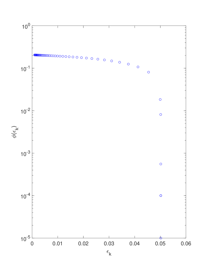
Fig. 3.2: The behavior of $\phi(\varepsilon)=x(\varepsilon)^{*}y(\varepsilon)$ for the matrix (3.27).

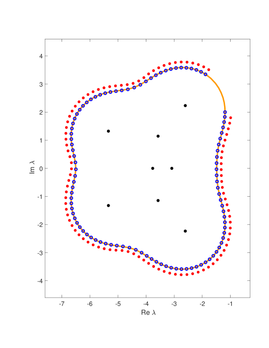
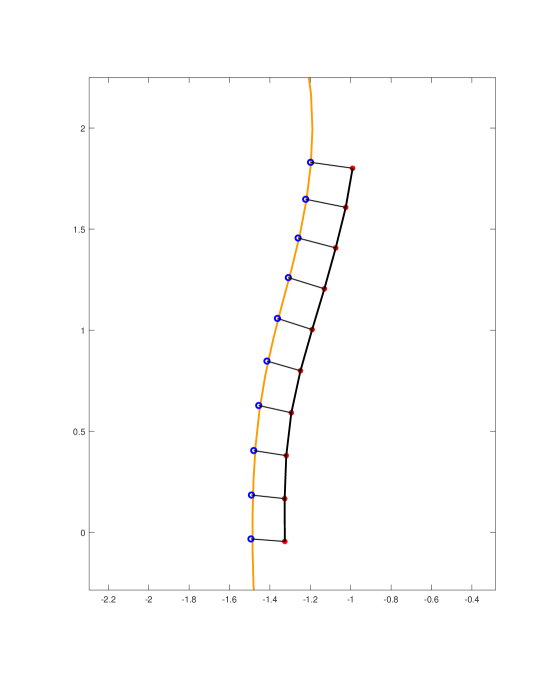
  Fig. 3.2: Boundary of the $\varepsilon$-pseudospectrum (continuous line) with $\varepsilon=1$ for the matrix $A$ in (II.3.19) with boundary points (circles) and control points (bullets) computed by the ladder algorithm (Algorithm 3.7). Right: zoom.

Numerical experiment.

We apply the ladder algorithm to the matrix $A$ in (II.3.19). Algorithm 3.7 produces the curve of circles in Figure 3.2 which is superimposed on the boundary of the $\varepsilon$-pseudospectrum (computed to high accuracy by Eigtool by Wright, ?). The average number of steps for each horizontal computation is $5.5$ for an accuracy tolerance ${\rm tol}=10^{-7}$.

III.4 Notes

Pseudospectra.

The standard reference for (complex unstructured) pseudospectra is the book by Trefethen & Embree (?). The notion of pseudospectrum was coined by Trefethen (?), but as noted there, the concept was used before under different names. The “approximate eigenvalues” of Varah (?) appear to be among the earliest precursors. Interpreting approximate eigenvalues or pseudospectral values as exact eigenvalues of a perturbed matrix is in the spirit of backward error analysis as pioneered by Wilkinson (?). In one of his last papers, Wilkinson (?) considered pseudospectra under the tentative name “fundamental inclusion domains”. Pseudospectra are of interest not only for matrices but more generally for linear operators on Hilbert or Banach spaces; see Trefethen (?) and also the concise account in the book by Davies (?), Chapter 9.

The motivating example of robust stability of a matrix (see Subsection III.1.1) was already studied by Van Loan (?) and Hinrichsen & Pritchard (?,?,?). They aim at determining the minimal norm of complex, real or structured perturbations that turn a stable matrix into an unstable one. This yields the (complex, real or structured) distance to instability, or stability radius, which equals the smallest perturbation size $\varepsilon$ for which the $\varepsilon$-pseudospectral abscissa becomes non-negative; this will be taken up in the next two chapters.

The fundamental Theorem III.1.2 and its proof via the distance to singularity was given by Wilkinson (?). Theorem III.1.4 on extremal complex perturbations is related to Guglielmi & Overton (?).

The use of pseudospectra together with the Cauchy integral formula to better understand the transient behaviour of dynamical systems was suggested by Trefethen (?). Subsection III.1.3 follows this approach, emphasizing the role of the pseudospectral abscissa and the stability radius. There are close connections to the Kreiss matrix theorem (Kreiss ?, LeVeque & Trefethen ? and Spijker ?) and to further stability bounds based on resolvent bounds as given, e.g., by Lubich & Nevanlinna (?), Reddy & Trefethen (?) and van Dorsselaer, Kraaijevanger & Spijker (?); see also Eisner (?) and references therein.

Pseudospectra of matrix pencils $A-\lambda B$ were studied by van Dorsselaer (?) and, e.g., Ahmad, Alam & Byers (?), structured pseudospectra for polynomial eigenvalue problems by Tisseur & Higham (?), and pseudospectra for rectangular matrices by Wright & Trefethen (?).

An extension of the concept of the $\varepsilon$-pseudospectrum of interest in control theory is the spectral value set that consists of the eigenvalues of all matrices $A+B\Delta(I-D\Delta)^{-1}C$ with given system matrices $A,B,C,D$ of compatible dimensions and with varying (complex or real or structured) matrices $\Delta$ of 2-norm at most $\varepsilon$. This was first considered (for $D=0$) by Hinrichsen and Kelb (?); see also Karow (?) for a detailed study and the book of Hinrichsen & Pritchard (?), Chapter 5. Apart from eigenvalues of $A$, the unstructured complex spectral value set contains all $\lambda\in\mathbb{C}$ for which the transfer matrix $H(\lambda)=C(\lambda I-A)^{-1}B+D$ has 2-norm at least $\varepsilon^{-1}$; see Guglielmi, Gürbüzbalaban & Overton (?). This characterization will be essential in Chapter VII.

Algorithms for computing the pseudospectral abscissa and radius.

The criss-cross algorithm of Burke, Lewis & Overton (?) for computing the pseudospectral abscissa relies on Byers’ lemma (Lemma III.2.1), due to Byers (?). This lemma is fundamental in that it relates singular values of a matrix shifted along a line parallel to the imaginary axis to the eigenvalues of a Hamiltonian matrix. This Hamiltonian connection has been put to important and enduring use in control systems starting with the work by Boyd, Balakrishnan & Kabamba (?); see e.g. Grivet-Talocia & Gustavsen (?) and references therein. We will encounter Hamiltonian eigenvalue optimization problems in Chapters VI and VII. Mengi & Overton (?) extended the criss-cross algorithm to computing the pseudospectral radius (using radial and circular searches), and Lu & Vandereycken (?) developed a criss-cross type algorithm for computing the real pseudospectral abscissa. Benner & Mitchell (?) studied criss-cross algorithms for computing the spectral value set abscissa and radius.

The rank-1 iteration of Guglielmi & Overton (?) for computing the pseudospectral abscissa and radius appears to be the first algorithm that uses the low-rank property of extremal perturbations as described by Theorem III.1.4. It motivated the rank-1 projected gradient flow algorithm of Guglielmi & Lubich (?) for computing the pseudospectral abscissa and radius, which opened up an approach to a wide range of eigenvalue optimization and matrix nearness problems, as discussed throughout this book.

Subspace acceleration approaches as used by Kressner & Vandereycken (?) also have a much wider scope than merely computing the pseudospectral abscissa; see, e.g., Kangal, Meerbergen, Mengi & Michiels (?) and Kressner, Lu & Vandereycken (?) for their use in other eigenvalue optimization problems.

In retrospect it appears remarkable how the modest aim of computing the pseudospectral abscissa led to the discovery of diverse classes of efficient algorithms that find use in a wide variety of other problems.

Computing the boundary of pseudospectra.

Trefethen (?) gave a survey of computing pseudospectra (as of 1999), which was then accompanied by the software package EigTool (Wright ?, Wright & Trefethen ?). The basic algorithm is based on a contour plot of the smallest singular value of $A-zI$ for $z$ on a grid. Algorithms for tracing boundary curves of complex pseudospectra were developed by Brühl (?) and Mezher & Philippe (?), and Bekas & Gallopoulos (?) combined curve-tracing and grids.

Guglielmi & Lubich (?) exploited the rank-1 property of extremal perturbations in curve-tracing algorithms. Those algorithms are related to the tangential–transversal algorithm and the ladder algorithm described in Section III.3, which have not previously appeared in the literature.

Chapter IV A two-level approach to matrix nearness problems

We formulate a two-level approach to matrix nearness problems whose wide scope will become apparent in the following chapters. In this short chapter we discuss the two-level algorithm in a setting related to the class of eigenvalue optimization problems of Chapter II. We then apply it to the particular problem of computing the stability radius:

• Given a matrix with all its eigenvalues having negative real part (a Hurwitz matrix), find the nearest complex matrix with some eigenvalue on the imaginary axis.

• Similarly, given a matrix with all its eigenvalues having modulus smaller than $1$ (a Schur matrix), find the nearest matrix with some eigenvalue on the complex unit circle.

Here, “nearest” will be understood to have minimal distance in the Frobenius norm. These problems can be conveniently rephrased in terms of pseudospectra: The stability radius of a Hurwitz matrix is the smallest $\varepsilon>0$ such that the $\varepsilon$-pseudospectrum has some point on the imaginary axis; and the stability radius of a Schur matrix is the smallest $\varepsilon>0$ such that the $\varepsilon$-pseudospectrum has some point on the unit circle. More generally, for a given matrix having all eigenvalues in an open set $\Omega$ in the complex plane, the problem is to find the smallest $\varepsilon>0$ such that the $\varepsilon$-pseudospectrum has some point on the boundary of $\Omega$.

The two-level approach taken here uses an inner iteration to compute the solution of an eigenvalue optimization problem as considered in Chapter II for a fixed perturbation size $\varepsilon$, and then determines the optimal perturbation size $\varepsilon_{\star}$ in an outer iteration.

The algorithm is not guaranteed to find the global optimum of these nonconvex and nonsmooth optimization problems, but it computes a matrix with the desired spectral property which is locally nearest and often, as observed in our numerical experiments, has a distance close to or equal to the minimal distance. It provides a rigorous upper bound to the minimal distance, and usually a very tight one. Running the algorithm with several different starting values reduces the risk of getting stuck in a local optimum.

IV.1 Two-level iteration

IV.1.1 Problem setting

We consider matrix nearness problems that are closely related to the eigenvalue optimization problems of Chapter II. For a given matrix $A\in\mathbb{C}^{n,n}$, let $\lambda(A)\in\mathbb{C}$ be a target eigenvalue of $A$. We again consider the smooth function $f(\lambda,\overline{\lambda})$ satisfying (II.1.2) that is to be minimized. For a prescribed real number $r$ in the range of $f$ we assume that

$$f(\lambda(A),\overline{\lambda}(A))>r,$$

so that for sufficiently small $\varepsilon>0$ we have $\phi(\varepsilon)>r$, where

$$\phi(\varepsilon):=\min\limits_{\Delta\in\mathbb{C}^{n,n},\,\|\Delta\|_{F}=\varepsilon}f\left(\lambda\left(A+\Delta\right),\overline{\lambda}\left(A+\Delta\right)\right).$$

The objective is to find the smallest $\varepsilon>0$ such that $\phi(\varepsilon)=r$:

$$\varepsilon_{\star}=\min\bigl{\{}\varepsilon>0\,:\,\phi(\varepsilon)\leq r\bigr{\}}.$$ (1.1)

Determining $\varepsilon_{\star}$ is a one-dimensional root-finding problem for the function $\phi$ that is defined by eigenvalue optimization problems as studied in Chapter II.

• (Stability radius of a Hurwitz matrix). With the function $f(\lambda,\overline{\lambda})=-\tfrac{1}{2}(\lambda+\overline{\lambda})=-{\mbox{\rm Re}}\,\lambda$ and $r=0$ and the target eigenvalue $\lambda(M)$ chosen as an eigenvalue of largest real part of a matrix $M$, we arrive at the classical problem of computing the stability radius (or distance to instability) $\varepsilon_{\star}$ of a Hurwitz matrix $A$, i.e. a matrix with negative spectral abscissa $\alpha(A)=\max\{{\mbox{\rm Re}}\,\lambda\,:\,\lambda\text{ is an eigenvalue of $A$}\}<0$ :

  $$\varepsilon_{\star}>0\quad\text{such that}\quad\alpha_{\varepsilon_{\star}}(A)=0,$$

  where $\alpha_{\varepsilon}(A)=\max\limits_{E\in\mathbb{C}^{n,n},\|E\|_{F}=1}\alpha(A+\varepsilon E)$ is the $\varepsilon$-pseudospectral abscissa (see the previous chapter).

  • (Stability radius of a Schur matrix). With $f(\lambda,\overline{\lambda})=-\lambda\overline{\lambda}=-|\lambda|^{2}$ and $r=-1$ and the target eigenvalue $\lambda(M)$ chosen as an eigenvalue of largest modulus of a matrix $M$, we arrive at the problem of computing the stability radius of a Schur matrix $A$, i.e. a matrix with spectral radius $\rho(A)=\max\{|\lambda|\,:\,\lambda\text{ is an eigenvalue of $A$}\}<1$ :

    $$\varepsilon_{\star}>0\quad\text{such that}\quad\rho_{\varepsilon_{\star}}(A)=1,$$

    where $\rho_{\varepsilon}(A)=\max\limits_{E\in\mathbb{C}^{n,n},\|E\|_{F}=1}\rho(A+\varepsilon E)$ is the $\varepsilon$-pseudospectral radius.

IV.1.2 Two-level iteration

Our approach is summarized by the following two-level method:

• Inner iteration: Given $\varepsilon>0$, we aim to compute a matrix $E(\varepsilon)\in\mathbb{C}^{n,n}$ of unit Frobenius norm, such that $F_{\varepsilon}(E)=f\left(\lambda\left(A+\varepsilon E\right),\overline{\lambda}\left(A+\varepsilon E\right)\right)$ is minimized, i.e.

  $$E(\varepsilon)=\arg\min\limits_{E\in\mathbb{C}^{n,n},\|E\|_{F}=1}F_{\varepsilon}(E).$$ (1.2)

• Outer iteration: We compute the smallest positive value $\varepsilon_{\star}$ with

  $$\phi(\varepsilon_{\star})=r,$$ (1.3)

  where $\phi(\varepsilon)=F_{\varepsilon}\left(E(\varepsilon)\right)=f\left(\lambda\left(A+\varepsilon E(\varepsilon)\right),\overline{\lambda}\left(A+\varepsilon E(\varepsilon)\right)\right)$.

IV.1.3 Inner iteration: Rank-1 constrained gradient flow

The eigenvalue optimization problem (1.2) is of the type studied in Chapter II, which has rank-1 matrices as optimizers (see Corollary II.II.3.1). To compute $E(\varepsilon)$ for a given $\varepsilon>0$, we make use of a constrained gradient system for the functional $F_{\varepsilon}(E)$ under the constraints of unit Frobenius norm of $E$ and $E\in\mathbb{C}^{n,n}$, which is further constrained to rank-1 matrices. We directly use the rank-1 constrained gradient flow approach developed in Chapter II, where we follow a suitable discretization of a rank-1 matrix differential equation (i.e., of a system of differential equations for two vectors) into a stationary point.

IV.1.4 Outer iteration: Derivative for the Newton step

In the outer iteration we compute $\varepsilon_{\star}$, the smallest positive solution of the one-dimensional root-finding problem (1.3). This can be solved by a variety of methods, such as bisection. We aim for a locally quadratically convergent Newton-type method, which can be justified under regularity assumptions that are generic. If these assumptions are not met, we can always resort to bisection. The algorithm proposed in the next subsection in fact uses a combined Newton–bisection approach.

In the following, an important role is again played by the gradient $G_{\varepsilon}(E)=2f_{\overline{\lambda}}xy^{*}$ as defined in Lemma II.II.2.1.

• For $\varepsilon$ close to $\varepsilon_{\star}$ and $\varepsilon<\varepsilon_{\star}$, we assume the following for the optimizer $E(\varepsilon)$ of (1.2):

  • The eigenvalue $\lambda(\varepsilon)=\lambda(A+\varepsilon E(\varepsilon))$ is a simple eigenvalue.

  • The map $\varepsilon\mapsto E(\varepsilon)$ is continuously differentiable.

  • The gradient $G(\varepsilon)=G_{\varepsilon}(E(\varepsilon))$ is nonzero.

Under this assumption, the branch of eigenvalues $\lambda(\varepsilon)$ and its corresponding eigenvectors $x(\varepsilon),y(\varepsilon)$ with the scaling (II.2.1) are also continuously differentiable functions of $\varepsilon$ in a left neighbourhood of $\varepsilon_{\star}$. We denote the eigenvalue condition number by

$$\kappa(\varepsilon)=\frac{1}{x(\varepsilon)^{*}y(\varepsilon)}>0.$$

The following result gives us an explicit and easily computable expression for the derivative of $\phi(\varepsilon)=F_{\varepsilon}(E(\varepsilon))=f(\lambda(\varepsilon),\overline{\lambda}(\varepsilon))$ with respect to $\varepsilon$ in terms of the gradient $G(\varepsilon)$.

• (Derivative for the Newton iteration).  Under Assumption IV.1.4, the function $\phi$ is continuously differentiable in a left neighbourhood of $\varepsilon_{\star}$ and its derivative is given as

  $$\phi^{\prime}(\varepsilon)=-\kappa(\varepsilon)\,\|G(\varepsilon)\|_{F}<0.$$ (1.4)

  • By Lemma II.II.2.1 and (II.2.4) we obtain, indicating by ^′ differentiation w.r.t. $\varepsilon$ and noting that $\frac{d}{d\varepsilon}(\varepsilon E(\varepsilon))=E(\varepsilon)+\varepsilon E^{\prime}(\varepsilon)$,

    $$\frac{1}{\kappa(\varepsilon)}\,\frac{d}{d\varepsilon}F_{\varepsilon}(E(\varepsilon))={\mbox{\rm Re}}\bigl{\langle}G(\varepsilon),E(\varepsilon)+\varepsilon E^{\prime}(\varepsilon)\bigr{\rangle}.$$ (1.5)

    By Theorem (II.II.2.3), we know that in the stationary point $E(\varepsilon)$, there exists a real $\mu(\varepsilon)$ such that

    $$E(\varepsilon)=\mu(\varepsilon)G(\varepsilon).$$ (1.6)

    Since $\|E(\varepsilon)\|_{F}=1$ for all $\varepsilon$, we find $1=|\mu(\varepsilon)|\,\|G(\varepsilon)\|_{F}$ (in particular $\mu(\varepsilon)\neq 0$) and

    $$0=\frac{1}{2}\frac{d}{d\varepsilon}\|E(\varepsilon)\|^{2}={\mbox{\rm Re}}\langle E(\varepsilon),E^{\prime}(\varepsilon)\rangle=\mu(\varepsilon)\,{\mbox{\rm Re}}\langle G(\varepsilon),E^{\prime}(\varepsilon)\rangle,$$

    so that

    $${\mbox{\rm Re}}\langle G(\varepsilon),E^{\prime}(\varepsilon)\rangle=0.$$

    Inserting this relation into (1.5) and using once again (1.6), we obtain

    $$\frac{1}{\kappa(\varepsilon)}\,\phi^{\prime}(\varepsilon)={\mbox{\rm Re}}\bigl{\langle}G(\varepsilon),E(\varepsilon)\bigr{\rangle}=\frac{1}{\mu(\varepsilon)}\|E(\varepsilon)\|_{F}^{2}=\frac{1}{\mu(\varepsilon)}={\rm sign}(\mu(\varepsilon))\,\|G(\varepsilon)\|_{F}.$$

    Since for $\varepsilon<\varepsilon_{\star}$, we have $\phi(\varepsilon)>\phi(\varepsilon_{\star})=r$, and since the above formula shows that $\phi^{\prime}$ cannot change sign, we must have $\phi^{\prime}(\varepsilon)<0$ and hence $\mu(\varepsilon)<0$. This yields the stated result.   $\sqcap$$\sqcup$

IV.1.5 Outer iteration: Newton–bisection method

In view of Theorem IV.1.4, applying Newton’s method to the equation $\phi(\varepsilon)=r$ yields the following iteration:

$$\varepsilon_{k+1}=\varepsilon_{k}+\frac{x(\varepsilon_{k})^{*}y(\varepsilon_{k})}{\|G(\varepsilon_{k})\|_{F}}\left(\phi(\varepsilon_{k})-r\right),$$ (1.7)

where the right-hand side uses the optimizer $E(\varepsilon_{k})$ computed by the inner iteration in the $k$-th step.

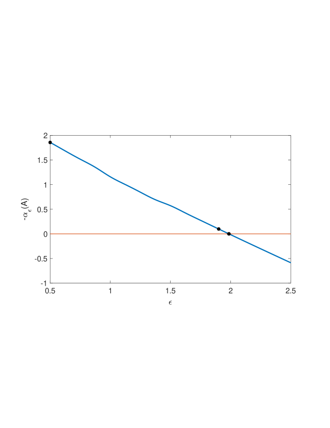
Fig. 1.1: The function $\phi(\varepsilon)=-\alpha_{\varepsilon}(A)$ for the matrix $A$ in (II.3.19). The bullets are the points computed by the outer iteration.

Data: Matrix $A$, matrix type (real/complex, structured)

$r>0$, ${\rm tol}_{0}$ (initial tolerance), $k_{\max}$ (max number of iterations)

$\varepsilon_{\rm lb}$ and $\varepsilon_{\rm ub}$ (starting values for the lower and upper bounds for $\varepsilon^{\star}$)

Result: $\varepsilon_{\star}$ (upper bound for the stability radius)

begin

   1 Set $\lambda(0)$ target eigenvalue of $A$, $x(0)$ and $y(0)$ the corresponding left and right eigenvectors of unit norm with $x(0)^{*}y(0)>0$.

   2 Initialize $E(\varepsilon_{0})$ according to the setting.

   3 Initialize $\varepsilon_{0}$ according to the setting.

    Set $k=0$.

   4 Initialize lower and upper bounds: $\varepsilon_{\rm lb}=0$, $\varepsilon_{\rm ub}=+\infty$.

    while $|\phi(\varepsilon_{k})-\phi(\varepsilon_{k-1})|<{\rm tol}_{k}$ do

      5 Compute $E(\varepsilon_{k})$, $\phi(\varepsilon_{k})$ by integrating the constrained gradient system with initial datum $E(\varepsilon_{k-1})$. (This is the inner iteration).

      6 Update upper and lower bounds $\varepsilon_{\rm lb}$, $\varepsilon_{\rm ub}$.

      7 if $\phi(\varepsilon_{k})<r$ then

         Set $\varepsilon_{\rm ub}=\min(\varepsilon_{\rm ub},\varepsilon_{k})$.

      else

         Set $\varepsilon_{\rm lb}=\max(\varepsilon_{\rm lb},\varepsilon_{k})$.

      8Compute $G(\varepsilon_{k})$.

      9 Compute $\varepsilon_{k+1}=\varepsilon_{k}+\displaystyle\frac{x(\varepsilon_{k})^{*}y(\varepsilon_{k})}{\|G(\varepsilon_{k})\|_{F}}\left(\phi(\varepsilon_{k})-r\right)$.

      10 Set $k=k+1$.

      11 if $\varepsilon_{k}\not\in[\varepsilon_{\rm lb},\varepsilon_{\rm ub}]$ then

         Set $\varepsilon_{k}=(\varepsilon_{\rm lb}+\varepsilon_{\rm ub})/2$.

      if $k=k_{\max}$ then

         goto $12$.

      else

         Set ${\rm tol}_{k}=\max\{10^{-2}\,{\rm tol}_{k-1},10^{-8}\}$.

      

      

   12if $k<k_{\max}$ then

      Set $\varepsilon_{\star}=\varepsilon_{k}$. Return $\varepsilon_{\star}$.

   else

      Print max number iterations reached

   

Algorithm 1.8 Outer iteration: Newton–bisection method

Algorithm 1.8 implements a hybrid Newton–bisection method that maintains an interval known to contain the root, bisecting when the Newton step is outside the interval $[\varepsilon_{\rm lb},\varepsilon_{\rm ub}]$.

Step 5 (in the while loop) gives the computational core of Algorithm 1.8; it implements the inner iteration and is not presented in detail since it depends on the possible structure of the matrix and on whether the low-rank structure is exploited. The inner iteration performs the algorithm to compute the extremal perturbation $E(\varepsilon_{k})$, as described in Chapter II. As input to the $k$-th iteration we use the factors of the final matrix $E$ computed for the previous value of $\varepsilon$ (this explains the choice of the initial datum at step 5).

The while loop after step 4 implements the outer iteration and makes use of a variable tolerance which decreases as $k$ increases, when the method is expected to approach convergence. A typical choice of ${\rm tol}_{0}$ is the norm of the difference of the first two iterates divided by $10$.

The factor $10^{-2}$ between two subsequent tolerances is fruit of an empirical experimentation and is motivated by the fact that we expect convergence - on the average - in about $4$ to $5$ iterates so that we reach the limit tolerance which is set here to $10^{-8}$. These numbers can naturally be considered as parameters of the code. Their choice here is only based on the experience with the numerical experiments we performed. When integrating numerically the gradient system with variable stepsize we are assured to fulfill the termination condition $|\phi(\varepsilon_{k})-\phi(\varepsilon_{k-1})|<{\rm tol}_{k}$ of the while loop because we are able to approximate the stationary point with prescribed accuracy. Due to the possible convergence of the inner method to a local instead of global minimum, the final value $\varepsilon_{\star}$ computed by Algorithm 1.8 might be larger than the minimal one.

IV.1.6 Outer iteration: Starting values

We make the following natural choice for the first initial datum $E_{0}$ (that is for the first value $\varepsilon=\varepsilon_{0}$): let $G_{0}$ be the gradient of $F_{\varepsilon}$ at $\varepsilon=0$, i.e., $G_{0}=2f_{\overline{\lambda}}xy^{*}$ with the target eigenvalue and its left and right eigenvectors for the unperturbed matrix $A$. We set

$$E_{0}=-\frac{G_{0}}{\|G_{0}\|},$$

which is the steepest descent direction at the unperturbed matrix for the functional $F_{\varepsilon}(E)$. At least for $\varepsilon_{0}$ not too large, this yields $F_{\varepsilon_{0}}(E_{0})<F_{0}$, where $F_{0}$ is the value assumed by the functional for the unperturbed matrix.

By formula (1.7), with $E(0)=E_{0}$, we formally apply the first Newton step and set

$$\varepsilon_{0}=\frac{x(0)^{*}y(0)}{\|G_{0}\|}(F_{0}-r).$$ (1.8)

While the above choice of starting values is reasonable when only a single trajectory is computed, it might in some problems be necessary to run several trajectories to reduce the risk of getting trapped in a local minimum.

IV.2 Computing the stability radius

The two-level approach of the previous section applies directly to computing the stability radius (or distance to instability) of a Hurwitz-stable matrix $A$. We choose the target eigenvalue $\lambda(M)$ as an eigenvalue of largest real part (among these, the one with largest imaginary part), and we take $f(\lambda,\overline{\lambda})=-\,{\mbox{\rm Re}}\,\lambda$ as the function to be minimized. The eigenvalue optimization problem (1.2) then becomes the maximization problem

$$E(\varepsilon)=\arg\max\limits_{E\in\mathbb{C}^{n,n},\|E\|_{F}=1}{\mbox{\rm Re}}\,\lambda(A+\varepsilon E),$$ (2.1)

and the optimal perturbation size $\varepsilon_{\star}$ is determined from Equation (1.3), which here reads

$${\mbox{\rm Re}}\,\lambda(A+\varepsilon_{\star}E(\varepsilon_{\star}))=0.$$ (2.2)

In the inner iteration, the eigenvalue optimization problem (2.1) is of the class studied in Chapter II with $f(\lambda,\overline{\lambda})=-{\mbox{\rm Re}}\,\lambda$ and is solved with the rank-1 constrained gradient flow approach developed there.

In the outer iteration we compute the optimal perturbation size $\varepsilon_{\star}$ by the Newton–bisection algorithm of Section IV.1.5 for $f(\lambda,\overline{\lambda})=-{\mbox{\rm Re}}\,\lambda$, using the derivative formula of Theorem II.IV.1.4 with $G=-xy^{*}$.

We consider a numerical example for the matrix $A$ in (II.3.19) with $\phi(\varepsilon)=-\alpha_{\varepsilon}(A)=-{\mbox{\rm Re}}\,\lambda(A+\varepsilon E(\varepsilon))$ (see Figure 1.1 and Table 2.1).

$k$	$\varepsilon_{k}$	$\phi(\varepsilon_{k})$	$\#$ eigs
​​​​ $0$	$0.5$	$1.856586036644719$	$43$
$1$	$1.901037794236803$	$0.098438736191212$	$53$
$2$	$1.985646225557732$	$0.000278151141277$	$47$
$3$	$1.985886638697453$	$0.000000000603666$	$1$

Table 2.1: Computation of the stability radius for the matrix $A$ in (II.3.19): computed values $\varepsilon_{k}$, $\phi(\varepsilon_{k})=-{\mbox{\rm Re}}\,\lambda(A+\varepsilon_{k}E_{k})$ and number of eigenvalue computations of the inner rank-$1$ algorithm.

IV.3 Notes

An early survey of matrix nearness problems, with emphasis on the properties of symmetry, positive definiteness, orthogonality, normality, rank-deficiency and instability, was given by Higham (?). His review is a source of continuing interest in view of the choice of topics and the references to the older literature.

Distance to instability (stability radius) under complex unstructured perturbations.

Van Loan (?) was apparently first to address the question “How near is a stable matrix to an unstable matrix?”. He considered both complex and real perturbations and came up with heuristic algorithms for approximating the smallest perturbations that shift an eigenvalue to the imaginary axis. His starting point was the characterization of the distance to instability under complex unstructured perturbations of the matrix $A$ as

$$\beta(A)=\min_{\omega\in\mathbb{R}}\,\sigma_{\min}(A-\mathrm{i}\omega I)$$ (3.1)

and an intricate characterization of the distance to instability under real perturbations.

For the complex case, Byers (?) showed that the Hamiltonian matrix

$$H(\sigma)=\begin{pmatrix}A&-\sigma I\\ \sigma I&A^{*}\end{pmatrix}$$

has a purely imaginary eigenvalue if and only if $\sigma\geq\beta(A)$; cf. Lemma III.III.2.1. Based on this result, he proposed a bisection method for computing the distance to the nearest complex matrix with an eigenvalue on the imaginary axis (the complex stability radius). Each step of the method requires the solution of an eigenvalue problem of the Hamiltonian matrix $H(\sigma)$ for varying $\sigma>0$. Byers (?) also gave an extension of the algorithm to compute the distance to the nearest complex matrix with an eigenvalue on the unit circle.

Conceptually related Hamiltonian eigenvalue methods by Boyd & Balakrishnan (?) and Bruinsma & Steinbuch (?) for the more general problem of computing the $\mathcal{H}_{\infty}$-norm of a transfer function also apply to computing the distance to stability. These methods converge locally quadratically.

He and Watson (?) developed a method for computing the distance to instability that is better suited for large sparse matrices $A$. They use a method based on inverse iteration for singular values to compute a stationary point of the function $f(\omega)=\sigma_{\min}(A-\mathrm{i}\omega I)$. They then check whether the stationary point reached is a global minimum by solving an eigenvalue problem for $H(\sigma)$. An alternative method for large sparse matrices was devised by Kressner (?) who worked with inverse iterations using sparse LU factorizations of imaginary shifts of Hamiltonian matrices $H(\sigma)$.

For $\sigma=\beta(A)$, the Hamiltonian matrix $H(\sigma)$ has an eigenvalue of even multiplicity on the imaginary axis. Generically, it is expected to be a defective double eigenvalue. Freitag & Spence (?) used a Newton-based method to find the parameters $\sigma$ and $\omega$ such that $H(\sigma)-\mathrm{i}\omega I$ has a zero eigenvalue corresponding to a two-dimensional Jordan block.

A different approach is to combine an algorithm for computing the $\varepsilon$-pseudospectral abscissa $\alpha_{\varepsilon}(A)$ (see Section III.2) with a root-finding algorithm for determining $\varepsilon_{\star}>0$ such that $\alpha_{\varepsilon_{\star}}(A)=0$. Then, $\varepsilon_{\star}$ is the distance to instability. This two-level approach can be used efficiently for large sparse matrices with the rank-1 iteration of Guglielmi & Overton (?), with the subspace method of Kressner & Vandereycken (?), and with the discretized rank-1 differential equation of Guglielmi & Lubich (?). The latter, differential equation based approach is described here in Section IV.1. It extends in a direct way to computing the distance to instability under real or structured perturbations, as will be described in the next chapter.

Chapter V Real and structured perturbations

In this chapter we extend the programme and algorithms of the previous chapters to the case where the matrix perturbations are restricted to be real or, more generally, to lie in a structure space $\mathcal{S}$, which is a given complex-linear or real-linear subspace of $\mathbb{C}^{n,n}$. For example, $\mathcal{S}$ may be a space of complex or real matrices with a given sparsity pattern, or of matrices with given range and co-range, or special matrices such as Hamiltonian or Toeplitz or Sylvester matrices. Remarkably, the rank-1 property of optimizers extends to general linear structures: optimizers of the structured eigenvalue optimization problem are the orthogonal projection of complex rank-1 matrices onto the structure space. This still enables us to work with rank-1 matrices to compute quantities related to structured pseudospectra such as the structured $\varepsilon$-pseudospectral abscissa, to trace the boundary of structured pseudospectra, and to adapt the two-level approach of the previous chapter to solve structured matrix nearness problems. In particular, we consider determining the following:

• the $\mathcal{S}$-structured stability radius (distance to instability) of a Hurwitz matrix $A$, i.e. finding a structured perturbation $\Delta\in\mathcal{S}$ of minimal norm such that $A+\Delta$ has some eigenvalue on the imaginary axis. This quantity assesses the robustness of asymptotic stability of linear differential equations under structured perturbations of the matrix;

• the $\mathcal{S}$-structured $\varepsilon$-stability radius of a Hurwitz matrix $A$, i.e. finding a structured perturbation $\Delta\in\mathcal{S}$ of minimal norm such that the (complex unstructured) pseudospectrum $\Lambda_{\varepsilon}(A+\Delta)$ has some point on the imaginary axis. This quantity will be shown to assess the robustness of transient bounds of linear differential equations under structured perturbations of the matrix;

• the $\mathcal{S}$-structured dissipativity radius of a matrix $A$ that has the numerical range in the open left complex half-plane. The aim is to find a structured perturbation $\Delta\in\mathcal{S}$ of minimal norm such that the numerical range of $A+\Delta$ has some point on the imaginary axis. The norm of $\Delta$ assesses the robustness of dissipativity $\|\exp(t(A+\Delta))\|_{2}\leq 1$ under structured perturbations $\Delta\in\mathcal{S}$;

• the $\mathcal{S}$-structured distance to singularity of an invertible matrix, i.e. finding a structured perturbation $\Delta\in\mathcal{S}$ of minimal norm such that $A+\Delta$ is singular. This is illustrated by the problem of finding a nearest pair of polynomials with a nontrivial common divisor to a given pair of polynomials that is coprime, which can be restated as a matrix nearness problem for Sylvester matrices.

For the first two items, we give two-level algorithms that use rank-1 matrix differential equations in the inner iteration and compute eigenvalues and eigenvectors of perturbed matrices in every step.

For the last two items, we present two-level algorithms with iterations that do not compute eigenvalues and eigenvectors (or singular values and singular vectors) but which still use rank-1 matrix differential equations in the inner iteration. In the third item we maximize the real part of Rayleigh quotients of perturbed matrices, and in the last item we minimize the squared Euclidean norm of perturbed matrices multiplying vectors. The resulting algorithms only need to compute matrix–vector products and inner products of vectors.

V.1 Real version of the eigenvalue optimization problem

V.1.1 Problem formulation

We now consider Problem (II.1.1) for a real matrix $A\in\mathbb{R}^{n,n}$ and real perturbations $\Delta\in\mathbb{R}^{n,n}$: find

$$\arg\min\limits_{\Delta\in\mathbb{R}^{n,n},\|\Delta\|_{F}=\varepsilon}f\left(\lambda\left(A+\Delta\right),\overline{\lambda}\left(A+\Delta\right)\right),$$ (1.1)

where again $\lambda(A+\Delta)$ is the target eigenvalue of the perturbed matrix $A+\Delta$, and $f$ satisfies (II.1.2). As in the complex case, it is convenient to write

$$\Delta=\varepsilon E\quad\mbox{ with }\ \|E\|_{F}=1$$

and to use the notation

$$F_{\varepsilon}(E)=f\left(\lambda\left(A+\varepsilon E\right),\overline{\lambda}\left(A+\varepsilon E\right)\right)$$ (1.2)

so that (1.1) can be rewritten as

$$\arg\min\limits_{E\in\mathbb{R}^{n,n},\|E\|_{F}=1}F_{\varepsilon}(E).$$ (1.3)

V.1.2 Norm-constrained gradient flow and rank of optimizers

The programme of Section II.2 extends to the real case with minor but important modifications.

Real gradient. Consider a smooth path of real matrices $E(t)\in\mathbb{R}^{n,n}$. Since $\dot{E}(t)$ is then also a real matrix, we have by Lemma II.2.1

$$\frac{1}{\varepsilon\kappa(t)}\,\frac{d}{dt}F_{\varepsilon}(E(t))=\bigl{\langle}G_{\varepsilon}^{\mathbb{R}}(E(t)),\dot{E}(t)\bigr{\rangle}$$ (1.4)

with the rescaled real gradient

$$G_{\varepsilon}^{\mathbb{R}}(E):={\mbox{\rm Re}}\,G_{\varepsilon}(E)={\mbox{\rm Re}}(2f_{\overline{\lambda}}\,xy^{*})\in\mathbb{R}^{n,n},$$ (1.5)

which is the real part of a complex rank-1 matrix and hence has rank at most $2$ (as a sum of two rank-1 matrices). As $\varepsilon$ is fixed and only the real case is considered in this section, we often write for short

$$G(E):=G_{\varepsilon}^{\mathbb{R}}(E).$$

Lemma II.2.2 on the direction of steepest admissible descent extends without ado to the real case: Consider real matrices and take everywhere the real inner product instead of the real part of the complex inner product.

Norm-constrained gradient flow. We consider the gradient flow on the manifold of real $n\times n$ matrices of unit Frobenius norm,

$$\dot{E}=-G(E)+\langle G(E),E\rangle E.$$ (1.6)

Monotonicity. Assuming simple eigenvalues along the trajectory, we then still have the monotonicity property of Theorem II.2.3,

$$\frac{d}{dt}F_{\varepsilon}(E(t))=-\|G(E)-\langle G(E),E\rangle E\|_{F}^{2}\leq 0,$$ (1.7)

with essentially the same proof (the real inner product replaces the real part of the complex inner product).

Stationary points. Also the characterization of stationary points as given in Theorem II.2.3 extends with the same proof: Let $E\in\mathbb{R}^{n,n}$ with $\|E\|_{F}=1$ be such that the eigenvalue $\lambda(A+\varepsilon E)$ is simple and $G_{\varepsilon}^{\mathbb{R}}(E)\neq 0$. Then,

$$E$$ is a stationary point of the differential equation (1.6) (1.8)

if and only if $$E G_{\varepsilon}^{\mathbb{R}}(E)$$ is a real multiple of .

As a consequence, optimizers of (1.3) have rank at most $2$. We can determine the precise rank as follows.

• (Rank of optimizers).  For $A\in\mathbb{R}^{n,n}$ and $\varepsilon>0$, let $E\in\mathbb{R}^{n,n}$ with $\|E\|_{F}=1$ be a stationary point of the differential equation (1.6) such that the eigenvalue $\lambda=\lambda(A+\varepsilon E)$ is simple and $G_{\varepsilon}^{\mathbb{R}}(E)\neq 0$. Then, $E$ is the real part of a complex rank-1 matrix and the rank of $E$ is as follows.

  •  If $\lambda$ is real, then $E$ has rank $1$.

  •  If ${\mbox{\rm Im}}\,\lambda\neq 0$, then $E$ has rank $2$.

  • (a) If $\lambda$ is real, then $f_{\lambda}$ is real and $x$ and $y$ can be chosen real, hence $G(E)={\mbox{\rm Re}}(\overline{f}_{\lambda}xy^{*})=f_{\lambda}xy^{\top}$ is of rank 1, and so is every nonzero real multiple, in particular $E$.

    (b) We set $w=f_{\lambda}y$ and separate the real and imaginary parts in $x=x_{R}+\mathrm{i}x_{I}$ and $w=w_{R}+\mathrm{i}w_{I}$. If ${\mbox{\rm Re}}(xw^{*})=x_{R}w_{R}^{\top}+x_{I}w_{I}^{\top}$ is of rank 1, then $x_{R}$ and $x_{I}$ are linearly dependent or $w_{R}$ and $w_{I}$ are linearly dependent. Let us first assume the former. In this case there is a real $\alpha$ such that $x=\cos(\alpha)v+\mathrm{i}\sin(\alpha)v$ for some nonzero real vector $v$. Rotating both $x$ and $y$ by ${\rm e}^{-\mathrm{i}\alpha}$ does not change the required property $x^{*}y>0$, so we can assume without loss of generality that $x$ is a real left eigenvector of the real matrix $A+\varepsilon E$, which implies that the corresponding eigenvalue $\lambda$ is real. The argument is analogous when $w_{R}$ and $w_{I}$ are linearly dependent.   $\sqcap$$\sqcup$

V.1.3 Low-rank matrices and their tangent matrices

Theorem V.1.2 motivates us to search for a differential equation on the manifold of real rank-2 matrices that has the same stationary points with non-real target eigenvalue as (1.6). For the stationary points with real target eigenvalues we use a differential equation for rank-1 matrices as in Section II.3.3.

In the following we consider differential equations on the manifold of real $n\times n$ matrices of rank $r$, denoted

$$\mathcal{M}_{r}=\mathcal{M}_{r}(\mathbb{R}^{n,n})=\{E\in\mathbb{R}^{n,n}\,:\,\text{rank}(E)=r\}.$$

While only ranks 1 and 2 are of interest for the optimization problem studied in this section, we now consider the case of a general fixed rank $r$, since it is not more complicated than rank 2 and will be useful later. We proceed similarly to the rank-1 case considered in Section II.3.2.

Every real rank-$r$ matrix $E$ of dimension $n\times n$ can be written in the form

$$E=USV^{\top}$$ (1.9)

where $U\in\mathbb{R}^{n,r}$ and $V\in\mathbb{R}^{n,r}$ have orthonormal columns, i.e.,

$$U^{\top}U=I_{r},\quad\ V^{\top}V=I_{r},$$ (1.10)

(with the identity matrix $I_{r}$ of dimension $r$), and $S\in\mathbb{R}^{r,r}$ is nonsingular. The singular value decomposition yields $S$ diagonal, but here we will not assume a special form of $S$. The representation (1.9) is not unique: replacing $U$ by $\widetilde{U}=UP$ and $V$ by $\widetilde{V}=VQ$ with orthogonal matrices $P,Q\in\mathbb{R}^{r,r}$, and correspondingly $S$ by $\widetilde{S}=P^{\top}SQ$, yields the same matrix $E=USV^{\top}=\widetilde{U}\widetilde{S}\widetilde{V}^{\top}$.

Every tangent matrix $\dot{E}\in T_{E}\mathcal{M}_{r}$ is of the form

$$\dot{E}=\dot{U}SV^{\top}+U\dot{S}V^{\top}+US\dot{V}^{\top},$$ (1.11)

where $\dot{S}\in\mathbb{R}^{r,r}$, and $U^{\top}\dot{U}$ and $V^{\top}\dot{V}$ are skew-symmetric (as results from differentiating $U^{\top}U=I_{r}$ and $V^{\top}V=I_{r}$). The matrices $\dot{S},\dot{U},\dot{V}$ are uniquely determined by $\dot{E}$ and $U,S,V$ if we impose the orthogonality conditions

$$U^{\top}\dot{U}=0,\quad\ V^{\top}\dot{V}=0.$$ (1.12)

Multiplying $\dot{E}$ with $U^{\top}$ from the left and with $V$ from the right, we then obtain

$$\dot{S}=U^{\top}\dot{E}V,\quad\dot{U}S=\dot{E}V-U\dot{S},\quad S{\dot{V}}^{\top}=U^{\top}\dot{E}-\dot{S}V^{\top},$$

which yields $\dot{S},\dot{U},\dot{V}$ in terms of $\dot{E}$. Extending this construction, we arrive at an explicit formula for the orthogonal projection onto the tangent space. Here, orthogonality refers to the real Frobenius inner product.

• (Rank-$r$ tangent space projection).  The orthogonal projection from $\mathbb{R}^{n,n}$ onto the tangent space $T_{E}\mathcal{M}_{r}$ at $E=USV^{\top}\in\mathcal{M}_{r}$ is given by

  $$P_{E}(Z)=Z-(I-UU^{\top})Z(I-VV^{\top})\quad\text{ for $Z\in\mathbb{C}^{n,n}$}.$$ (1.13)

  • The proof is a direct extension of the proof of Lemma II.3.2. Let $P_{E}(Z)$ be defined by (1.13). Determining (similarly to above) $\dot{S},\dot{U},\dot{V}$ by

    $$\dot{S}=U^{\top}ZV,\quad\dot{U}S=ZV-U\dot{S},\quad S{\dot{V}}^{\top}=U^{\top}Z-\dot{S}V^{\top},$$

    we obtain $P_{E}(Z)=UU^{\top}ZVV^{\top}-ZVV^{\top}-UU^{\top}Z$ in the form (1.11) with (1.12) and hence

    $$P_{E}(Z)\in T_{E}\mathcal{M}_{r}.$$

    Furthermore,

    $$\langle P_{E}(Z),\dot{E}\rangle=\langle Z,\dot{E}\rangle\qquad\text{for all }\ \dot{E}\in T_{E}\mathcal{M}_{r},$$

    because $\langle(I-UU^{\top})Z(I-VV^{\top}),\dot{E}\rangle=\langle Z,(I-UU^{\top})\dot{E}(I-VV^{\top})\rangle=0$ by (1.11). Hence, $P_{E}(Z)$ is the orthogonal projection of $Z$ onto $T_{E}\mathcal{M}_{r}$.   $\sqcap$$\sqcup$

    We note that $P_{E}(E)=E$ for $E\in\mathcal{M}_{r}$, or equivalently, $E\in T_{E}\mathcal{M}_{r}$.

V.1.4 Rank-constrained gradient flow

In the differential equation (1.6) we replace the right-hand side by its orthogonal projection onto $T_{E}\mathcal{M}_{r}$, so that solutions starting with rank $r$ will retain rank $r$ for all times:

$$\dot{E}=P_{E}\Bigl{(}-G(E)+\langle G(E),E\rangle E\Bigr{)}.$$ (1.14)

Since $E\in T_{E}\mathcal{M}_{r}$, we have $P_{E}(E)=E$ and $\langle E,Z\rangle=\langle E,P_{E}(Z)\rangle$, and hence the differential equation can be rewritten as

$$\dot{E}=-P_{E}(G(E))+\langle E,P_{E}(G(E))\rangle E,$$ (1.15)

which differs from (1.6) only in that $G(E)$ is replaced by its orthogonal projection to $T_{E}\mathcal{M}_{r}$. This shows that $\langle E,\dot{E}\rangle=0$, so that the unit norm of $E$ is conserved along solutions of (1.14).

To obtain the differential equation in a form that uses the factors in $E=USV^{\top}$ rather than the full $n\times n$ matrix $E$, we use the following result, which follows directly from the proof of Lemma V.1.3.

• (Differential equations for the factors).  For $E=USV^{\top}\in\mathcal{M}_{r}$ with nonsingular $S\in\mathbb{R}^{r,r}$ and with $U\in\mathbb{R}^{n,r}$ and $V\in\mathbb{R}^{n,r}$ having orthonormal columns, the equation $\dot{E}=P_{E}(Z)$ is equivalent to $\dot{E}=\dot{U}SV^{\top}+U\dot{S}V^{\top}+US\dot{V}^{\top},$ where

  $$\dot{S} = U^{\top}ZV$$

  $$\dot{U} = (I-UU^{\top})ZVS^{-1}$$ (1.16)

  $$\dot{V} = (I-VV^{\top})Z^{\top}US^{-\top}.$$

  With $Z=-G(E)+\langle G(E),E\rangle E$ and $r=2$, this yields that the differential equation (1.14) for $E=USV^{\top}$ is equivalent to a system of differential equations for $S,U,V$. On the right-hand side appears the inverse of the matrix $S$, which may be ill-conditioned. In the present context, this appears when the target eigenvalue gets close to the real axis (see Theorem V.1.2) so that $E$, and hence $S$, becomes almost of rank $1$. In such a situation of a small singular value in $S$, standard numerical integrators become unstable or yield plainly wrong numerical solutions unless used with a tiny stepsize proportional to the smallest nonzero singular value. Later in this section we will describe a numerical integrator that is robust to small singular values.

Monotonicity.

Assuming simple eigenvalues almost everywhere along the trajectory, we still have the monotonicity property of Theorem II.3.3 along solutions $E(t)$ of (1.14),

$$\frac{d}{dt}F_{\varepsilon}(E(t))=-\|P_{E}(G(E))-\langle E,P_{E}(G(E))\rangle E\|_{F}^{2}\leq 0,$$ (1.17)

with essentially the same proof (the real inner product replaces the real part of the complex inner product).

Stationary points.

Comparing the differential equations (1.6) and (1.14) immediately shows that every stationary point of (2.8) is also a stationary point of the projected differential equation (1.14). As in Theorem II.3.3, the converse is also true for the stationary points $E$ of unit Frobenius norm with ${P_{E}(G(E))\neq 0}$. This shows that the low-rank projection does not create spurious stationary points.

• (Stationary points).  Let $E\in\mathcal{M}_{2}$ be of unit Frobenius norm and assume that $P_{E}(G(E))\neq 0$. If $E$ is a stationary point of the projected differential equation (1.14), then $E$ is already a stationary point of the differential equation (1.6).

  • The proof extends the proof of Theorem II.3.3. We show that $E$ is a real multiple of $G_{\varepsilon}(E)$. By (1.8), $E$ is then a stationary point of the differential equation (2.8).

    For a stationary point $E$ of (1.14), we must have equality in (3.11), which shows that $P_{E}(G)$ (with $G=G(E)$ for short) is a nonzero real multiple of $E$. Hence, in view of $P_{E}(E)=E$, we can write $G$ as

    $$G=\mu E+W,\quad\text{ where $\mu\neq 0$ is real and $P_{E}(W)=0$.}$$

    With $E=USV^{\top}$ as above, we then have

    $$W=W-P_{E}(W)=(I-UU^{\top})W(I-VV^{\top}).$$

    Since $G$ is of rank at most $2$, it can be written in the form $G=XRY^{\top}$, where $X,Y\in\mathbb{R}^{n,2}$ have orthonormal columns and $R\in\mathbb{R}^{2,2}$. So we have

    $$XRY^{\top}=\mu USV^{\top}+(I-UU^{\top})W(I-VV^{\top}).$$

    Multiplying from the right with $V$ yields $X(RY^{\top}V)=\mu US$, which shows that $X$ has the same range as $U$, and multiplying from the left with $U^{\top}$ yields that $Y$ has the same range as $V$. Hence, $G$ has the same range and corange as $E$, which implies that $P_{E}(G)=G$. Since we already know that $P_{E}(G)$ is a nonzero real multiple of $P_{E}(E)=E$, it follows that $G$ is the same real multiple of $E$. By (1.8), $E$ is therefore a stationary point of (1.6).   $\sqcap$$\sqcup$

    As in Remark II.3.3, it is shown that if $G(E)$ is of rank 2 and $P_{E}(G(E))=0$, then it follows that $Ey=0$ and $x^{*}E=0$, which implies that $\lambda$ is already an eigenvalue of the unperturbed matrix $A$ with the same eigenvectors $x$ and $y$, which is a very exceptional situation.

V.1.5 Time-stepping for the low-rank differential equation

A robust integrator.

The following method adapts the low-rank integrator of Ceruti & Lubich (?) to the norm-constrained situation considered here. It first updates the basis matrices $U$ and $V$ with orthonormal columns in parallel and then uses a Galerkin approximation to the differential equation (1.14) in the updated basis. This basis update and Galerkin (BUG) integrator has been shown to be robust to the presence of small singular values, which would here appear in the case of a target eigenvalue near the real axis.

One time step of integration from time $t_{k}$ to $t_{k+1}=t_{k}+h$ starting from a factored rank-$r$ matrix $E_{k}=U_{k}S_{k}V_{k}^{\top}$ of unit Frobenius norm computes an updated rank-$r$ factorization $E_{k+1}=U_{k+1}S_{k+1}V_{k+1}^{\top}$ of unit Frobenius norm as follows.

1. Update the basis matrices $U_{k}\rightarrow U_{k+1}$ and $V_{k}\rightarrow V_{k+1}$:
   Integrate from $t=t_{k}$ to $t_{k+1}=t_{k}+h$ the $n\times r$ matrix differential equation

   $$\dot{K}(t)=-G(K(t)V_{k}^{\top})V_{k},\qquad K(t_{k})=U_{k}S_{k}.$$

   Perform a QR factorization $K(t_{k+1})=U_{k+1}{R}_{k+1}$ and compute the $r\times r$ matrix $M=U_{k+1}^{\top}U_{k}$.
   Integrate from $t=t_{k}$ to $t_{k+1}$ the $n\times r$ matrix differential equation

   $$\dot{L}(t)=-G(U_{k}L(t)^{\top})^{\top}U_{k},\qquad L(t_{k})=V_{k}{S}_{k}^{\top}.$$

   Perform a QR factorization $L(t_{k+1})=V_{k+1}\widetilde{R}_{k+1}$ and compute the $r\times r$ matrix $N=V_{k+1}^{\top}V_{k}$.
   

2. Update ${S}_{k}\rightarrow{S}_{k+1}$ :
   Integrate from $t=t_{k}$ to $t_{k+1}$ the $r\times r$ matrix differential equation

   $$\dot{S}(t)=-U_{k+1}^{\top}G(U_{k+1}S(t)V_{k+1}^{\top})V_{k+1},\qquad S(t_{k})=\frac{M{S}_{k}N^{\top}}{\|M{S}_{k}N^{\top}\|_{F}},$$

   and set ${S}_{k+1}=S(t_{k+1})/\|S(t_{k+1})\|_{F}$.

The differential equations in the substeps are solved approximately by a step of some standard numerical integrator, e.g. the explicit Euler method or better a low-order explicit Runge–Kutta method such as the second-order Runge method. We denote the result of the fully discrete method with stepsize $h$ as $U(h)$, $V(h)$, $S(h)$.

Step-size selection.

As in Section II.3.4, the stepsize selection is done by an Armijo-type strategy. Along solutions $E(t)\in\mathcal{M}_{2}$ of (1.14), we have by (1.4)–(1.5)

$$\frac{d}{dt}F_{\varepsilon}(E(t))=-g(E(t))\quad\text{ with }\quad g(E)=\varepsilon\kappa\bigl{(}\|P_{E}(G)\|_{F}^{2}-\langle G,E\rangle^{2}\bigr{)}\geq 0$$

where $\kappa=1/(x^{*}y)>0$, $G=G_{\varepsilon}^{\mathbb{R}}(E)={\mbox{\rm Re}}(2f_{\overline{\lambda}}xy^{*})$ with the normalized left and right eigenvectors $x$ and $y$ to the eigenvalue $\lambda(A+\varepsilon E)$.

We note that on separating real and imaginary parts in $2f_{\overline{\lambda}}x=w_{R}+\mathrm{i}w_{I}$ and $y=y_{R}+\mathrm{i}y_{I}$ and defining the $n\times 2$ real matrices $W=(w_{R},w_{I})$ and $Y=(y_{R},y_{I})$, we have the real factorization

$$G=WY^{\top}.$$

With the rank-2 matrix $E=USV^{\top}$ in factorized form as above, we can then compute $g(E)$ without actually forming the $n\times n$ matrices $E$ and $G$: noting that with the $2\times 2$ matrices $P=U^{\top}W$ and $Q=V^{\top}Y$ we have

$$\langle G,E\rangle=\langle WY^{\top},USV^{\top}\rangle=\langle PQ^{\top},S\rangle_{\mathbb{R}^{2\times 2}}$$

and

$$P_{E}(G)=UPY^{\top}-UPQ^{\top}V^{\top}+WQ^{\top}V^{\top},$$

which yields after a straightforward computation

$$\|P_{E}(G)\|_{F}^{2}=\|PY^{\top}\|_{F}^{2}+\|WQ^{\top}\|_{F}^{2}-\|PQ^{\top}\|_{F}^{2},$$

so that finally $g=g(E)$ is given by

$$g=\varepsilon\kappa\bigl{(}\|PY^{\top}\|_{F}^{2}+\|WQ^{\top}\|_{F}^{2}-\|PQ^{\top}\|_{F}^{2}-\langle PQ^{\top},S\rangle^{2}\bigr{)}.$$ (1.18)

With this quantity $g$, the Armijo-type stepsize selection is then done as in Section II.3.4. A time step of the method is summarized in Algorithm 1.9.

Data: $A,\varepsilon,\theta>1,U_{k}\approx U(t_{k}),V_{k}\approx V(t_{k})\in\mathbb{R}^{n\times 2}$ with orthonormal columns, $S_{k}\approx S(t_{k})\in\mathbb{R}^{2\times 2}$ of unit Frobenius norm, target eigenvalue $\lambda_{k}=\lambda(A+\varepsilon U_{k}S_{k}V_{k}^{\top})$, $h_{k}$ (proposed step size)

Result: $U_{k+1},V_{k+1},S_{k+1}$, $\lambda_{k+1}$, $h_{k+1}$

begin

   1 Initialize the step size by the proposed step size, $h=h_{k}$

   2 Compute $f_{k}=f(\lambda_{k},\overline{\lambda_{k}})$

   3 Compute the left/right eigenvectors $x_{k},y_{k}$ to $\lambda_{k}$ such that $\|x_{k}\|=\|y_{k}\|=1,x_{k}^{*}y_{k}>0$

   4 Compute $g_{k}$ by (1.18)

   5 Initialize $f(h)=f_{k}$

    while $f(h)\geq f_{k}$ do

      6 Compute $U(h),V(h),S(h)$ by the above rank-2 integrator

      7 Compute $\lambda(h)$ target eigenvalue of $A+\varepsilon U(h)S(h)V(h)^{\top}$

      8 Compute $f(h)=f\bigl{(}\lambda(h),\overline{\lambda(h)}\bigr{)}$

       if $f(h)\geq f_{k}$ then

         Reduce the step size, $h:=h/\theta$

      

   9Initialize $h_{\rm next}=h$

    if $f(h)\geq f_{k}-(h/\theta)g_{k}$ then

      Reduce the step size for the next step, $h_{\rm next}:=h/\theta$

   if $h_{\rm next}=h_{k}$ then

      10Compute $U(\theta h),V(\theta h),S(\theta h)$ by the above rank-2 integrator

      11 Compute $\lambda(\theta h)$ target eigenvalue of $A+\varepsilon U(\theta h)S(\theta h)V(\theta h)^{\top}$

      12 Compute $f(\theta h)=f\bigl{(}\lambda(\theta h),\overline{\lambda(\theta h)}\bigr{)}$

       if $f(h)>f(\theta h)$ then

         Enlarge the step size for the next step, $h:=\theta h$ and then $h_{\rm next}:=h$

      

   13Set $h_{k+1}=h_{\rm next}$, $\lambda_{k+1}=\lambda(h)$, and the starting values for the next step as $U_{k+1}=U(h)$, $V_{k+1}=V(h)$, $S_{k+1}=S(h)$

    return

Algorithm 1.9 Integration step for the rank-2 constrained real gradient system

V.2 Structured eigenvalue optimization problems

V.2.1 Problem formulation. Complex- and real-linear structures

Let the structure space $\mathcal{S}$ be a complex-linear or real-linear subspace of $\mathbb{C}^{n,n}$, e.g. a space of complex or real matrices with a prescribed sparsity pattern, or with prescriped range and co-range, or Toeplitz matrices, or Hamiltonian matrices, etc.

As before, we set with the target eigenvalue $\lambda(M)$

$$F_{\varepsilon}(E)=f\left(\lambda\left(A+\varepsilon E\right),\overline{\lambda}\left(A+\varepsilon E\right)\right).$$ (2.1)

We now restrict the admissible perturbations $\varepsilon E$ to be in $\mathcal{S}$ and consider the structured eigenvalue optimization problem to find

$$\arg\min\limits_{E\in\mathcal{S},\|E\|_{F}=1}F_{\varepsilon}(E).$$ (2.2)

V.2.2 Orthogonal projection onto the structure

Let $\Pi^{\mathcal{S}}$ be the orthogonal projection (w.r.t. the Frobenius inner product) onto $\mathcal{S}$: for every $Z\in\mathbb{C}^{n,n}$,

$$\Pi^{\mathcal{S}}Z\in\mathcal{S}\quad\text{ and }\quad{\mbox{\rm Re}}\langle\Pi^{\mathcal{S}}Z,W\rangle={\mbox{\rm Re}}\langle Z,W\rangle\quad\text{for all }\,W\!\in\mathcal{S}.$$ (2.3)

For a complex-linear subspace $\mathcal{S}$, taking the real part of the complex inner product can be omitted (because with $W\in\mathcal{S}$, then also $\mathrm{i}W\in\mathcal{S}$), but taking the real part is needed for real-linear subspaces. In the following examples, the stated action of $\Pi^{\mathcal{S}}$ is readily verified.

• (Real matrices). For $\mathcal{S}=\mathbb{R}^{n,n}$, we have $\Pi^{\mathcal{S}}Z={\mbox{\rm Re}}\,Z$ for all $Z\in\mathbb{C}^{n,n}$.

  • (Sparse matrices). If $\mathcal{S}$ is the space of complex matrices with a prescribed sparsity pattern, then $\Pi^{\mathcal{S}}Z$ leaves the entries of $Z$ on the sparsity pattern unchanged and annihilates those outside the sparsity pattern. If $\mathcal{S}$ is the space of real matrices with a prescribed sparsity pattern, then $\Pi^{\mathcal{S}}Z$ takes the real part of the entries of $Z$ on the sparsity pattern and annihilates those outside the sparsity pattern.

    • (Matrices with prescribed range and co-range). An example of particular interest in control theory is the perturbation space

      $$\mathcal{S}=\{B\Delta C\,:\,\Delta\in\mathbb{R}^{k,l}\},$$

      where $B\in\mathbb{R}^{n,k}$ and $C\in\mathbb{R}^{l,n}$ with $k,l<n$ are given matrices of full rank. Here, $\Pi^{\mathcal{S}}Z=BB^{\dagger}ZC^{\dagger}C$, where $B^{\dagger}$ and $C^{\dagger}$ are the Moore–Penrose inverses of $B$ and $C$, respectively.

      • (Toeplitz matrices). If $\mathcal{S}$ is the space of complex $n\times n$ Toeplitz matrices, then $\Pi^{\mathcal{S}}Z$ is obtained by replacing in each diagonal all the entries of $Z$ by their arithmetic mean. For real Toeplitz matrices, the same action is done on ${\mbox{\rm Re}}\,Z$.

        • (Hamiltonian matrices). If $\mathcal{S}$ is the space of $2d\times 2d$ real Hamiltonian matrices, then $\Pi^{\mathcal{S}}Z=J^{-1}\mathrm{Sym}({\mbox{\rm Re}}(JZ))$, where $\mathrm{Sym}(\cdot)$ takes the symmetric part of a matrix and

          $$J=\begin{pmatrix}0&I_{d}\\ -I_{d}&0\end{pmatrix},$$

          for which $J^{-1}=J^{\top}=-J$. We recall that a real matrix $A$ is Hamiltonian if $JA$ is symmetric.

V.2.3 Structure- and norm-constrained gradient flow

The programme of Chapter II extends to structured cases as follows.

Structured gradient.

Consider a smooth path of structured matrices $E(t)\in\mathcal{S}$. Since then also $\dot{E}(t)\in\mathcal{S}$, we have by Lemma II.II.2.1

$$\frac{1}{\varepsilon\kappa(t)}\,\frac{d}{dt}F_{\varepsilon}(E(t))={\mbox{\rm Re}}\,\bigl{\langle}G_{\varepsilon}^{\mathcal{S}}(E(t)),\dot{E}(t)\bigr{\rangle}$$ (2.4)

with the rescaled structured gradient

$$G_{\varepsilon}^{\mathcal{S}}(E):=\Pi^{\mathcal{S}}G_{\varepsilon}(E)=\Pi^{\mathcal{S}}(2f_{\overline{\lambda}}\,xy^{*})\in\mathcal{S},$$ (2.5)

where $x,y$ are the left and right eigenvectors, normalized to unit norm and with positive inner product, associated with a simple eigenvalue $\lambda$ of $A+\varepsilon E$, and $f_{\overline{\lambda}}=(\partial f/\partial\overline{\lambda})(\lambda,\overline{\lambda})$.

We note that $G_{\varepsilon}^{\mathcal{S}}(E)$ is the orthogonal projection onto $\mathcal{S}$ of a rank-1 matrix.

Lemma II.II.2.2 on the direction of steepest admissible descent extends immediately to the structured case: If $E,G\in\mathcal{S}$ in Lemma II.II.2.2, then also $Z_{\star}$ of (II.2.7) is in $\mathcal{S}$.

Norm- and structure-constrained gradient flow.

We consider the gradient flow on the manifold of structured $n\times n$ matrices in $\mathcal{S}$ of unit Frobenius norm,

$$\dot{E}=-G_{\varepsilon}^{\mathcal{S}}(E)+{\mbox{\rm Re}}\langle G_{\varepsilon}^{\mathcal{S}}(E),E\rangle E.$$ (2.6)

Monotonicity.

Assuming simple eigenvalues along the trajectory, we then still have the monotonicity property of Theorem II.2.3,

$$\frac{d}{dt}F_{\varepsilon}(E(t))\leq 0,$$ (2.7)

with essentially the same proof.

Stationary points.

Also the characterization of stationary points as given in Theorem II.2.3 extends with the same proof: Let $E\in\mathcal{S}$ with $\|E\|_{F}=1$ be such that the eigenvalue $\lambda(A+\varepsilon E)$ is simple and $G_{\varepsilon}^{\mathcal{S}}(E)\neq 0$. Then,

$$E$$ is a stationary point of the differential equation (2.6) (2.8)

if and only if $$E G_{\varepsilon}^{\mathcal{S}}(E)$$ is a real multiple of .

Before we proceed in this direction, we take a look at the condition $G_{\varepsilon}^{\mathcal{S}}(E)\neq 0$. We have the following result.

• (Non-vanishing structured gradient).  Let $A,E\in\mathcal{S}$ and $\varepsilon>0$, and let $\lambda$ be a simple target eigenvalue of $A+\varepsilon E$.

(i) Complex case: $\mathcal{S}$ is a complex-linear subspace of $\mathbb{C}^{n,n}$. Then,

$$G_{\varepsilon}^{\mathcal{S}}(E)\neq 0\quad\text{ if }\quad\overline{\lambda}f_{\overline{\lambda}}\neq 0.$$

(ii) Real case: $\mathcal{S}$ is a real-linear subspace of $\mathbb{R}^{n,n}$. Then,

$$G_{\varepsilon}^{\mathcal{S}}(E)\neq 0\quad\text{ if }\quad{\mbox{\rm Re}}(\overline{\lambda}f_{\overline{\lambda}})\neq 0.$$

We emphasize that also $A$ needs to be in $\mathcal{S}$. The result does not hold true when $A\notin\mathcal{S}$.

• We give the proof for the real case. The complex case is analogous but slightly simpler. We take the real inner product of $G_{\varepsilon}^{\mathcal{S}}(E)$ with $A+\varepsilon E\in\mathcal{S}$ and use the definition (2.5) of $G_{\varepsilon}^{\mathcal{S}}(E)$:

  $$\langle G_{\varepsilon}^{\mathcal{S}}(E),A+\varepsilon E\rangle={\mbox{\rm Re}}\langle\Pi^{\mathcal{S}}(2f_{\overline{\lambda}}\,xy^{*}),A+\varepsilon E\rangle={\mbox{\rm Re}}\langle 2f_{\overline{\lambda}}\,xy^{*},A+\varepsilon E\rangle$$

  $$={\mbox{\rm Re}}\bigl{(}2f_{\lambda}\,x^{*}(A+\varepsilon E)y\bigr{)}={\mbox{\rm Re}}\bigl{(}2f_{\lambda}\lambda\,x^{*}y\bigr{)}=2\,{\mbox{\rm Re}}\bigl{(}f_{\overline{\lambda}}\overline{\lambda}\bigr{)}\,(x^{*}y),$$

  where $x^{*}y>0$. This yields the result.   $\sqcap$$\sqcup$

If the identity matrix $I$ is in $\mathcal{S}$, then the condition for $G_{\varepsilon}^{\mathcal{S}}(E)\neq 0$ can be weakened:

– In the complex case, it then suffices to have $f_{\overline{\lambda}}\neq 0$. This is seen by taking the inner product with $A+\varepsilon E-\mu I\in\mathcal{S}$ for an arbitrary $\mu\in\mathbb{C}$.

– In the real case, if $\lambda$ is real, then it suffices to have ${\mbox{\rm Re}}\,f_{\overline{\lambda}}\neq 0$. If $\lambda$ is non-real, then it even suffices to have $f_{\overline{\lambda}}\neq 0$. In both cases this is seen by taking the inner product with $A+\varepsilon E-\mu I\in\mathcal{S}$ for an arbitrary $\mu\in\mathbb{R}$.

V.2.4 Rank-1 matrix differential equation

As a consequence of (2.8), optimizers of (2.2) are projections onto $\mathcal{S}$ of rank-1 matrices. This motivates us to search for a differential equation on the manifold of rank-$1$ matrices that leads to the same stationary points.

Solutions of (2.6) can be written as $E(t)=\Pi^{\mathcal{S}}Z(t)$ where $Z(t)$ solves

$$\dot{Z}=-G_{\varepsilon}(E)+{\mbox{\rm Re}}\langle G_{\varepsilon}(E),E\rangle Z\quad\text{ with }\ E=\Pi^{\mathcal{S}}Z.$$ (2.9)

We note that ${\mbox{\rm Re}}\langle E,\dot{E}\rangle=0$ if $\|E\|_{F}=1$, so that the unit Frobenius norm of $E(t)$ is conserved for all $t$. As every solution tends to a stationary point of rank 1, we project the right-hand side onto the tangent space $T_{Y}\mathcal{M}_{1}$ at $Y$ of the manifold of complex rank-1 matrices $\mathcal{M}_{1}=\mathcal{M}_{1}(\mathbb{C}^{n,n})$ and consider instead the projected differential equation with solutions of rank 1:

$$\dot{Y}=-P_{Y}G_{\varepsilon}(E)+{\mbox{\rm Re}}\langle P_{Y}G_{\varepsilon}(E),E\rangle Y\quad\text{ with }\ E=\Pi^{\mathcal{S}}Y.$$ (2.10)

Note that then

$$\dot{E}=-\Pi^{\mathcal{S}}P_{Y}G_{\varepsilon}(E)+{\mbox{\rm Re}}\langle\Pi^{\mathcal{S}}P_{Y}G_{\varepsilon}(E),E\rangle E\quad\text{ with }\ E=\Pi^{\mathcal{S}}Y,$$ (2.11)

which differs from the gradient flow (2.6) only in that the gradient $G_{\varepsilon}(E)$ is replaced by the rank-1 projected gradient $P_{Y}G_{\varepsilon}(E)$.

For $E=\Pi^{\mathcal{S}}Y$ of unit Frobenius norm,

$${\mbox{\rm Re}}\langle E,\dot{E}\rangle={\mbox{\rm Re}}\langle E,\dot{Y}\rangle=-{\mbox{\rm Re}}\langle E,P_{Y}G_{\varepsilon}(E)\rangle+{\mbox{\rm Re}}\langle P_{Y}G_{\varepsilon}(E),E\rangle\,{\mbox{\rm Re}}\langle E,Y\rangle=0,$$

where we used that ${\mbox{\rm Re}}\langle E,Y\rangle={\mbox{\rm Re}}\langle E,\Pi^{\mathcal{S}}Y\rangle={\mbox{\rm Re}}\langle E,E\rangle=\|E\|_{F}^{2}=1$. So we have

$$\|E(t)\|_{F}=1\qquad\text{for all }t.$$

We write a rank-1 matrix $Y\in\mathcal{M}_{1}$ in a non-unique way as

$$Y=\rho uv^{*},$$

where $\rho\in\mathbb{R},\ \rho>0$ and $u,v\in\mathbb{C}^{n}$ have unit norm. The following lemma extends Lemma II.II.3.3 to the structured situation. It shows how the rank-1 differential equation (2.10) can be restated in terms of differential equations for the factors $u,v$ and an explicit formula for $\rho$.

• (Differential equations for the factors).  Every solution $Y(t)\in\mathcal{M}_{1}$ of the rank-1 differential equation (2.10) with $\|\Pi^{\mathcal{S}}Y(t)\|_{F}=1$ can be written as $Y(t)=\rho(t)u(t)v(t)^{*}$ where $u(t)$ and $v(t)$ of unit norm satisfy the differential equations

  $$\rho\dot{u} =-\displaystyle\tfrac{\mathrm{i}}{2}{\mbox{\rm Im}}(u^{*}Gv)u-(I-uu^{*})Gv,\qquad$$

  $$\rho\dot{v} =-\displaystyle\tfrac{\mathrm{i}}{2}{\mbox{\rm Im}}(v^{*}Gu)v-(I-vv^{*})G^{*}u,$$

  where $G=G_{\varepsilon}(E)$ for $E=\Pi^{\mathcal{S}}Y=\rho\,\Pi^{\mathcal{S}}(uv^{*})$ and $\rho=1/\|\Pi^{\mathcal{S}}(uv^{*})\|_{F}$.

  We find that with the exception of the additional positive factor $\rho$ on the left-hand side, these differential equations are of the same form as in Lemma II.II.3.3. Note that $\rho$ is only related to the speed with which a trajectory is percursed, but does not affect the trajectory itself. However, here $G=G_{\varepsilon}(E)$ for a different matrix $E=\Pi^{\mathcal{S}}(\rho uv^{*})$ instead of $E=uv^{*}$ in (II.(3.8)).

• The equation for $\rho$ is obvious because $1=\|E\|_{F}=\|\Pi^{\mathcal{S}}(\rho uv^{*})\|_{F}=\rho\|\Pi^{\mathcal{S}}(uv^{*})\|_{F}$.
  We write the right-hand side of (2.10) and use (3.3) to obtain for $Y=\rho uv^{*}$

  $$\dot{Y} =-P_{Y}G+{\mbox{\rm Re}}\langle P_{Y}G,E\rangle Y$$

  $$=-\ (I-uu^{*})Gvv^{*}-uu^{*}G(I-vv^{*})-uu^{*}Gvv^{*}+{\mbox{\rm Re}}\Big{\langle}P_{Y}G,E\Big{\rangle}Y$$

  $$=-\ \Bigl{(}(I-uu^{*})Gvv^{*}+\tfrac{\mathrm{i}}{2}{\mbox{\rm Im}}(u^{*}Gv)u\Bigr{)}v^{*}-u\Bigl{(}u^{*}G(I-vv^{*})+\tfrac{\mathrm{i}}{2}{\mbox{\rm Im}}(u^{*}Gv)v^{*}\Bigr{)}$$

  $$\quad\,-\Bigl{(}{\mbox{\rm Re}}(u^{*}Gv)+{\mbox{\rm Re}}\langle P_{Y}G,E\rangle\rho\Bigr{)}uv^{*}.$$

  Since this is equal to $\dot{Y}=(\rho\dot{u})v^{*}+u(\rho\dot{v}^{*})+\dot{\rho}uv^{*}$, we can equate $\rho\dot{u}$, $\rho\dot{v}^{*}$ and $\dot{\rho}$ with the three terms in big brackets. So we obtain the stated differential equations for $u$ and $v$ (and another one for $\rho$, which will not be needed). Further we have $(d/dt)\|u\|^{2}=2\,{\mbox{\rm Re}}(u^{*}\dot{u})=0$ and analogously for $v$, which yields that $u$ and $v$ stay of unit norm.   $\sqcap$$\sqcup$

  We note that for $G=G_{\varepsilon}(E)=2f_{\overline{\lambda}}\,xy^{*}$ (see Lemma II.II.2.1) and with $\alpha=u^{*}x$, $\beta=v^{*}y$ and $\gamma=2f_{\overline{\lambda}}$, we obtain differential equations that differ from (II.3.9) only in the additional factor $\rho$ on the left-hand side:

  $$\begin{array}[]{rcl}\rho\dot{u}&=&\alpha\overline{\beta}\gamma\,u-\overline{\beta}\gamma\,x-\tfrac{\mathrm{i}}{2}\,{\mbox{\rm Im}}(\alpha\overline{\beta}\gamma)u\\[8.53581pt] \rho\dot{v}&=&\overline{\alpha}\beta\overline{\gamma}\,v-\overline{\alpha\gamma}\,y-\tfrac{\mathrm{i}}{2}\,{\mbox{\rm Im}}(\overline{\alpha}\beta\overline{\gamma})v.\end{array}$$ (2.12)

Stationary points.

The following theorem states that under some non-degeneracy conditions (see Remark II.II.3.3), the differential equations (2.6) and (2.10) yield the same stationary points.

• (Relating stationary points).  (a) Let $E\in\mathcal{S}$ of unit Frobenius norm be a stationary point of the gradient system (2.6) that satisfies $\Pi^{\mathcal{S}}G_{\varepsilon}(E)\neq 0$. Then, $E=\Pi^{\mathcal{S}}Y$ for an $Y\in\mathbb{C}^{n,n}$ of rank $1$ that is a stationary point of the differential equation (2.10).

  (b) Conversely, let $Y\in\mathbb{C}^{n,n}$ of rank $1$ be a stationary point of the differential equation (2.10) such that $E=\Pi^{\mathcal{S}}Y$ has unit Frobenius norm and $P_{Y}G_{\varepsilon}(E)\neq 0$. Then, $E$ is a stationary point of the gradient system (2.6).

  • Let $G=G_{\varepsilon}(E)$ in this proof for short.

    (a) By (2.8), $E=\mu^{-1}\Pi^{\mathcal{S}}G$ for some nonzero real $\mu$. Then, $Y:=\mu^{-1}G$ is of rank 1 and we have $E=\Pi^{\mathcal{S}}Y$. We further note that $P_{Y}G=\mu P_{Y}Y=\mu Y=G$. We thus have

    $$-P_{Y}G+{\mbox{\rm Re}}\langle P_{Y}G,E\rangle Y=-G+{\mbox{\rm Re}}\langle G,E\rangle Y.$$

    Here we find that

    $${\mbox{\rm Re}}\langle G,E\rangle={\mbox{\rm Re}}\langle\Pi^{\mathcal{S}}G,E\rangle={\mbox{\rm Re}}\langle\mu E,E\rangle=\mu\|E\|_{F}^{2}=\mu.$$

    So we have

    $$-G+{\mbox{\rm Re}}\langle G,E\rangle Y=-G+\mu Y=0$$

    by the definition of $Y$. This shows that $Y$ is a stationary point of (2.10).

    (b) By the argument used in the proof of Theorem II.3.3, stationary points $Y\in\mathcal{M}_{1}$ of the differential equation (2.10) are characterized as real multiples of $G$. Hence, $E=\Pi^{\mathcal{S}}Y$ is a real multiple of $\Pi^{\mathcal{S}}G$, and by (2.8), $E=\Pi^{\mathcal{S}}Y$ is a stationary point of (2.6).   $\sqcap$$\sqcup$

Possible loss of global monotonicity and preservation of local monotonicity near stationary points.

Since the projections $\Pi^{\mathcal{S}}$ and $P_{Y}$ do not commute, we cannot guarantee the monotonicity (2.7) along solutions of (2.10). However, in all our numerical experiments we observed a monotonic decrease of the functional in all steps except possibly (and rarely) in the first step. In the following we will explain this monotonic behaviour locally near a stationary point, but we have no theoretical explanation for the numerically observed monotonic behaviour far from stationary points.

The first observation, already made in the proof of Theorem V.2.4, is that at a stationary point $Y$ of (2.10), we have $P_{Y}G_{\varepsilon}(E)=G_{\varepsilon}(E)$ for $E=\Pi^{\mathcal{S}}Y$. Therefore, close to a stationary point, $P_{Y}G_{\varepsilon}(E)$ will be close to $G_{\varepsilon}(E)$. It turns out that it is even quadratically close. This is made more precise in the following lemma.

• (Projected gradient near a stationary point).  Let $Y_{\star}\in\mathcal{M}_{1}$ with $E_{\star}=\Pi^{\mathcal{S}}Y_{\star}\in\mathcal{S}$ of unit Frobenius norm. Let $Y_{\star}$ be a stationary point of the rank-1 projected differential equation (2.10), with an associated target eigenvalue $\lambda$ of $A+\varepsilon E_{\star}$ that is simple. Then, there exist $\bar{\delta}>0$ and a real $C$ such that for all positive $\delta\leq\bar{\delta}$ and all $Y\in\mathcal{M}_{1}$ with $\|Y-Y_{\star}\|\leq\delta$ and associated $E=\Pi^{\mathcal{S}}Y$ of unit norm, we have

  $$\|P_{Y}G_{\varepsilon}\left(E\right)-G_{\varepsilon}\left(E\right)\|\leq C\delta^{2}.$$ (2.13)

  • We consider a smooth path $Y(\tau)=u(\tau)v(\tau)^{*}\in\mathcal{M}_{1}$ (with $u(\tau),v(\tau)\in\mathbb{C}^{n}$) and associated $E(\tau)=\Pi^{\mathcal{S}}Y(\tau)$ of unit Frobenius norm with initial value

    $$Y(0)=Y_{\star}=\mu^{-1}G_{\star}\quad\mbox{\rm for some nonzero real}\ \mu\quad\mbox{and}$$

    $$G_{\star}=G_{\varepsilon}\left(E_{\star})\right)=2\overline{f}_{\lambda}xy^{*},$$

    where $E_{\star}=\Pi^{\mathcal{S}}Y_{\star}$ is of unit Frobenius norm and $(\lambda,x,y)$ is the target eigentriplet of $A+\varepsilon E_{\star}$ associated with the target eigenvalue $\lambda$.

    A direct calculation of the first-order terms in the Taylor expansions of $P_{Y(\tau)}G_{\varepsilon}(E(\tau))$ and $G_{\varepsilon}(E(\tau))$, which uses the formula (II.3.3) for the projection $P_{Y(\tau)}$ and the formula (II.2.3) of the rescaled gradient $G_{\varepsilon}(E(\tau))$, surprisingly yields that the Taylor expansions of $P_{Y(\tau)}G_{\varepsilon}(E(\tau))$ and $G_{\varepsilon}(E(\tau))$ at $\tau=0$ coincide up to $O(\tau^{2})$. This gives the stated result.   $\sqcap$$\sqcup$

    As a direct consequence of this lemma, a comparison of the differential equations (2.11) and (2.6) yields that $\delta$-close to a stationary point, the functional decreases monotonically along solutions of (2.10) up to $O(\delta^{2})$, and even with the same negative derivative as for the gradient flow (2.6) up to $O(\delta^{2})$. Note that the derivative of the functional is proportional to $-\delta$ in a $\delta$-neighbourhood of a strong local minimum. Guglielmi, Lubich & Sicilia (?) use Lemma V.2.4 to prove a result on local convergence as $t\to\infty$ to strong local minima of the functional $F_{\varepsilon}$ of (1.4) for $E(t)=\Pi^{\mathcal{S}}Y(t)$ of unit Frobenius norm associated with solutions $Y(t)$ of the rank-1 differential equation (2.10).

V.2.5 Discrete algorithm

Since the differential equations for $u$ and $v$ have essentially the same form as in the unstructured case, the splitting algorithm of Subsection II.3.4 extends in a straightforward way, and also the stepsize selection is readily extended. We refer to Guglielmi, Lubich & Sicilia (?) for details of the algorithm and for numerical experiments with sparse matrices and matrices perturbed with matrices of given rank and co-rank.

V.3 Structured pseudospectra

V.3.1 Motivation and definitions

We take up the motivating example for the $\varepsilon$-pseudospectrum of a matrix $A$ and consider the linear dynamical system $\dot{x}(t)=Ax(t)$. We now ask if asymptotic stability is preserved under real or structured perturbations $\Delta\in\mathcal{S}$ of norm bounded by a given $\varepsilon>0$. This question is answered by the sign of the $\mathcal{S}$-structured $\varepsilon$-pseudospectral abscissa defined as

$$\alpha_{\varepsilon}^{\mathcal{S}}(A)=\max\{{\mbox{\rm Re}}\,\lambda:\ \ \Delta\in\mathcal{S} \|\Delta\|\leq\varepsilon$$ There exists with such that

$$\text{$\lambda$ is an eigenvalue of $A+\Delta$}\}.$$

This number is computed by solving a problem (1.1) for $\mathcal{S}=\mathbb{R}^{n,n}$, or (2.1)–(2.2) for an arbitrary complex-linear or real-linear structure space $\mathcal{S}$, in each case with the function to be minimized given by $f(\lambda,\overline{\lambda})=-\tfrac{1}{2}(\lambda+\overline{\lambda})=-{\mbox{\rm Re}}\,\lambda$.

It is useful to rephrase the question in terms of the $\varepsilon$-pseudospectrum, which is defined as follows.

• The $\mathcal{S}$-structured $\varepsilon$-pseudospectrum of the matrix $A$ is the set

  $$\Lambda_{\varepsilon}^{\mathcal{S}}(A)=\{\lambda\in\mathbb{C}:\ \ \text{$\lambda\in\Lambda(A+\Delta)$ for some $\Delta\in\mathcal{S}$ with $\|\Delta\|\leq\varepsilon$}\},$$ (3.1)

  where $\Lambda(M)\subset\mathbb{C}$ denotes the spectrum of a square matrix $M$.

  For $\mathcal{S}=\mathbb{C}^{n,n}$, $\Lambda_{\varepsilon}(A)=\Lambda_{\varepsilon}^{\mathbb{C}}(A)=\Lambda_{\varepsilon}^{\mathcal{S}}(A)$ is the complex $\varepsilon$-pseudospectrum, and for $\mathcal{S}=\mathbb{R}^{n,n}$, $\Lambda_{\varepsilon}^{\mathbb{R}}(A)=\Lambda_{\varepsilon}^{\mathcal{S}}(A)$ is known as the real $\varepsilon$-pseudospectrum.

  The $\mathcal{S}$-structured $\varepsilon$-pseudospectral abscissa of the matrix $A$ can then be rewritten more compactly as

  $$\alpha_{\varepsilon}^{\mathcal{S}}(A)=\max\{{\mbox{\rm Re}}\,\lambda:\ \lambda\in\Lambda_{\varepsilon}^{\mathcal{S}}(A)\}.$$ (3.2)

  An analogous quantity for discrete-time linear dynamical systems $x_{k+1}=Ax_{k}$ is the $\mathcal{S}$-structured $\varepsilon$-pseudospectral radius of the matrix $A$,

  $$\rho_{\varepsilon}^{\mathcal{S}}(A)=\max\{|\lambda|:\ \lambda\in\Lambda_{\varepsilon}^{\mathcal{S}}(A)\}.$$ (3.3)

V.3.2 Extremal structured perturbations

For structured pseudospectra, there is no characterization in terms of singular value decompositions or resolvent bounds. There is, however, an analogue of Theorem III.III.1.4 which characterizes extremal perturbations, at least at boundary points $\lambda\in\partial\Lambda_{\varepsilon}^{\mathcal{S}}(A)$ where the boundary is differentiable and thus admits an outer normal ${\rm e}^{\mathrm{i}\theta}$.

• (Extremal structured perturbations).  Let $\lambda\in\partial\Lambda_{\varepsilon}^{\mathcal{S}}(A)$ be on a smooth section of the boundary, with outer normal ${\rm e}^{\mathrm{i}\theta}$ at $\lambda$. Let $\Delta\in\mathcal{S}$ of Frobenius norm $\varepsilon$ be such that $A+\Delta$ has $\lambda$ as a simple eigenvalue. Let $x$ and $y$ be left and right eigenvectors of $A+\Delta$ to the eigenvalue $\lambda$, of unit norm and with $x^{*}y>0$. If the matrix $\Pi^{\mathcal{S}}({\rm e}^{\mathrm{i}\theta}xy^{*})$ is non-zero, where $\Pi^{\mathcal{S}}$ is the orthogonal projection (2.3) onto $\mathcal{S}$, then

  $$\Delta=\varepsilon\,\eta\,\Pi^{\mathcal{S}}({\rm e}^{\mathrm{i}\theta}xy^{*}),$$

  where $\eta=1/\|\Pi^{\mathcal{S}}({\rm e}^{\mathrm{i}\theta}xy^{*})\|_{F}>0$.

  • The proof is based on Section V.2.3, in particular (2.8). In the proof we denote the given $\lambda\in\partial\Lambda_{\varepsilon}^{\mathcal{S}}(A)$ as $\lambda_{0}$ and use $\lambda$ to denote a complex variable. Similarly, we denote the matrix $\Delta$ in the statement of the lemma by $\Delta_{0}$ and use $\Delta$ for a generic matrix in $\mathcal{S}$.

    We set $\mu=\lambda_{0}+\delta{\rm e}^{\mathrm{i}\theta}$ with a small $\delta>0$. For the function

    $$f(\lambda,\overline{\lambda})=|\mu-\lambda|^{2}=(\mu-\lambda)(\overline{\mu}-\overline{\lambda})$$

    we consider the optimization problem (2.2) with $\lambda(A+\Delta)$ denoting the eigenvalue of $A+\Delta$ closest to $\lambda_{0}$, which has $\Delta_{0}=\varepsilon E_{0}$ with $\|E_{0}\|_{F}=1$ as a solution, and $\lambda(A+\Delta_{0})=\lambda_{0}$. In particular, $E_{0}$ is then a stationary point of the gradient system (2.6) and hence satisfies (2.8) with a negative factor as in (II.2.13), which yields that $E_{0}$ is a negative real multiple of the structured gradient $G_{\varepsilon}^{\mathcal{S}}(E_{0})=\Pi^{\mathcal{S}}(f_{\overline{\lambda}}xy^{*})$ with $f_{\overline{\lambda}}=\partial f/\partial\overline{\lambda}(\lambda_{0},\overline{\lambda}_{0})=-(\mu-\lambda_{0})=-\delta{\rm e}^{\mathrm{i}\theta}$, which yields $\Delta_{0}$ as stated. This holds under the condition that $G_{\varepsilon}^{\mathcal{S}}(E_{0})\neq 0$ is non-zero, i.e., $\Pi^{\mathcal{S}}({\rm e}^{\mathrm{i}\theta}xy^{*})\neq 0$.   $\sqcap$$\sqcup$

    • In the unstructured real case $\mathcal{S}=\mathbb{R}^{n,n}$, where $\Pi^{\mathcal{S}}(Z)={\mbox{\rm Re}}\,Z$, the condition ${\mbox{\rm Re}}({\rm e}^{\mathrm{i}\theta}xy^{*})\neq 0$ excludes sections of $\partial\Lambda_{\varepsilon}^{\mathbb{R}}(A)$ that consist of intervals on the real line.

V.3.3 Tracing the boundary of structured pseudospectra

Structured ladder algorithm.

The ladder algorithm of Section III.3.2 is readily extended to compute smooth sections of the boundary of the structured $\varepsilon$-pseudospectrum of a given matrix for a general linear structure $\mathcal{S}$:

Let $\lambda_{0}\in\partial\Lambda_{\varepsilon}^{\mathcal{S}}(A)$ be a simple eigenvalue of $A+\varepsilon\eta_{0}\Pi^{\mathcal{S}}(u_{0}v_{0}^{*})$ (with $u_{0}$ and $v_{0}$ of unit norm and $\eta_{0}=1/\|\Pi^{\mathcal{S}}(u_{0}v_{0}^{*})\|$) that lies on a smooth section of $\partial\Lambda_{\varepsilon}^{\mathcal{S}}(A)$, with outer normal ${\rm e}^{\mathrm{i}\theta_{0}}=|u_{0}^{*}v_{0}|/(u_{0}^{*}v_{0})$ at $\lambda_{0}$, as follows from Theorem V.3.2.

With a small distance $\delta>0$, we define the nearby point $\mu_{0}$ on the straight line normal to $\partial\Lambda_{\varepsilon}(A)$ at $\lambda_{0}$,

$$\mu_{0}=\lambda_{0}+\delta{\rm e}^{\mathrm{i}\theta_{0}}.$$

We add a tangential component, either to the left ($+$) or to the right ($-$),

$$\mu_{1}=\mu_{0}\pm\mathrm{i}\delta{\rm e}^{\mathrm{i}\theta_{0}}.$$

We then apply the structured eigenvalue optimization algorithm of Section V.2 for the function

$$f(\lambda,\overline{\lambda})=(\lambda-\mu_{1})(\overline{\lambda}-\overline{\mu_{1}})=|\lambda-\mu_{1}|^{2},$$

choosing $E_{0}=\Pi^{\mathcal{S}}(u_{0}v_{0}^{*})$ as the starting iterate. That algorithm aims to compute $u_{1}$ and $v_{1}$ of unit norm such that $A+\varepsilon\Pi^{\mathcal{S}}(u_{1}v_{1}^{*})$ has the boundary point $\lambda_{1}\in\partial\Lambda_{\varepsilon}^{\mathcal{S}}(A)$ nearest to $\mu_{1}$ as an eigenvalue. At the point $\lambda_{1}$ we have the outer normal $(\mu_{1}-\lambda_{1})/|\mu_{1}-\lambda_{1}|$.

We continue from $\lambda_{1}$ and $u_{1}$, $v_{1}$ in the same way as above, constructing a sequence $\lambda_{k}$ ($k\geq 1$) of points on the boundary of the structured pseudospectrum $\Lambda_{\varepsilon}^{\mathcal{S}}(A)$ with approximate spacing $\delta$.

Let us consider here some illustrative examples, in which we apply this structured version of the ladder algorithm.

Real pseudospectra

We consider the real matrix in (II.3.19) and $\varepsilon=1$ and are interested in computing the boundary of the real $\varepsilon$-pseudospectrum $\Lambda_{\varepsilon}^{\mathbb{R}}(A)$. In Figure 3.1 we show a section of the real $\varepsilon$-pseudospectrum of $A$ with $\varepsilon=1$, as computed with the ladder algorithm, together with the boundary of the complex $\varepsilon$-pseudospectrum $\Lambda_{\varepsilon}(A)$. Note that in the plot of the set $\Lambda_{\varepsilon}^{\mathbb{R}}(A)$, there are two missing real segments, which are readily obtained by intersecting the complex $\varepsilon$-pseudospectrum and the real axis.

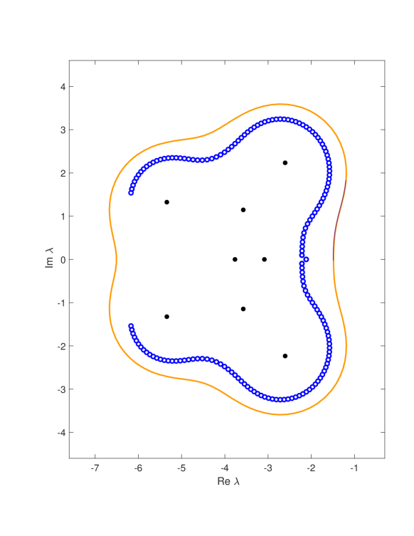
Fig. 3.1: Section of the boundary of the boundary of $\Lambda_{\varepsilon}^{\mathbb{R}}(A)$ computed by the ladder algorithm compared with the unstructured pseudospectrum $\Lambda_{\varepsilon}(A)$.

Hamiltonian pseudospectra

We show an example of a real Hamiltonian $\varepsilon$-pseudospectrum, $\Lambda_{\varepsilon}^{\mathcal{H}}(H)$ for $\mathcal{H}=\text{Ham}(\mathbb{R}^{n,n})$ the space of $n\times n$ real Hamiltonian matrices. Let

$$H=\left(\begin{array}[]{rrrr}1.0&1.6&1.2&0.4\\ 2.2&-0.6&0.4&-4.4\\ -4.0&-7.4&-1.0&-2.2\\ -7.4&6.0&-1.6&0.6\end{array}\right)$$ (3.4)

and set $\varepsilon=0.4$. In Figure 3.2 we show the whole set of boundary points of $\Lambda_{\varepsilon}^{\mathcal{S}}(H)$ as computed by the ladder algorithm.

 

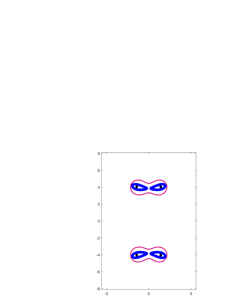
Fig. 3.2: Boundary points on the real Hamiltonian $\varepsilon$-pseudospectrum $\Lambda_{\varepsilon}^{\mathcal{H}}(H)$ computed by the ladder algorithm versus the complex unstructured pseudospectrum $\Lambda_{\varepsilon}(H)$.

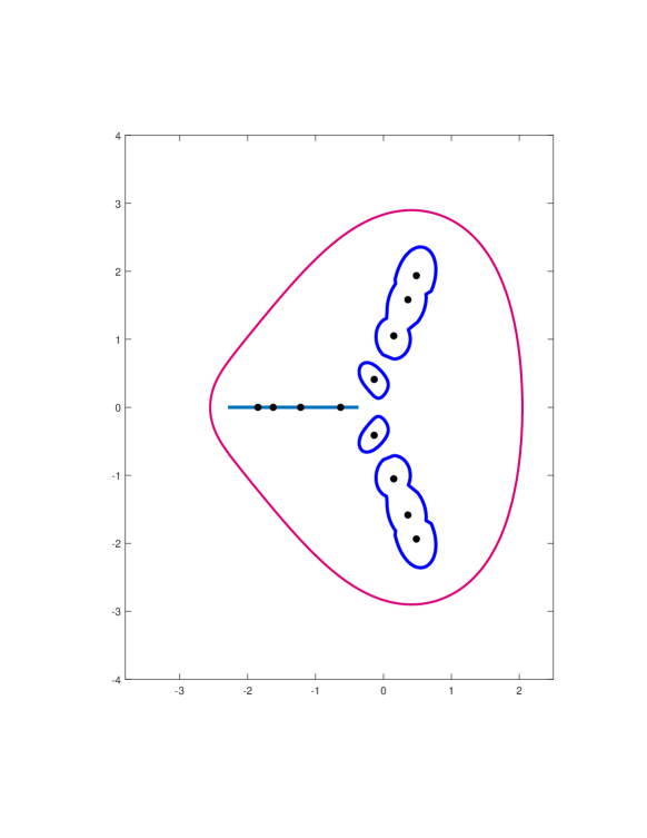
Fig. 3.3: The penta-diagonal real Toeplitz-structured $\varepsilon$-pseudospectrum $\Lambda_{\varepsilon}^{\mathcal{T}_{5}}(T)$, as computed by the ladder algorithm, inside the unstructured $\varepsilon$-pseudospectrum.

Toeplitz pseudospectra

We further consider the case of Toeplitz matrices, for which – as far as we know – there are no available tools to draw structured pseudospectra and compute related quantities. We denote by $\mathcal{T}_{k}$ the space of $k$-diagonal real Toeplitz matrices and $\Lambda_{\varepsilon}^{{\mathcal{T}}_{k}}(A)$ the associated structured $\varepsilon$-pseudospectrum.

We consider the $12\times 12$ penta-diagonal Toeplitz matrix

$$T=T_{5}(s_{1},s_{2},d,t_{1},t_{2})\in\mathcal{T}_{5},$$ (3.5)

that is the matrix with elements

$$a_{i,i}=d,\qquad i=1,\ldots,n$$

$$a_{i+1,i}=s_{1},\qquad i=1,\ldots,n-1$$

$$a_{i+2,i}=s_{2},\qquad i=1,\ldots,n-2$$

$$a_{i-1,i}=t_{1},\qquad i=1,\ldots,n-1$$

$$a_{i-2,i}=t_{2},\qquad i=1,\ldots,n-2.$$

with entries $d=-0.3$, $s_{1}=-0.1$, $s_{2}=-0.3$, $t_{1}=2$, $t_{2}=0.5$. We use the ladder algorithm to compute the $\mathcal{T}_{5}$-structured $\varepsilon$-pseudospectrum of $T$ for $\varepsilon=0.6$. In Figure 3.3 we show both the structured and the unstructured pseudospectra. The so obtained structured $\varepsilon$ pseudospectrum agrees with what is obtained by intensive sampling of eigenvalues of perturbed matrices $A+\varepsilon E$ with $E\in\mathcal{S}$ of Frobenius norm at most 1.

V.4 Computing the structured stability radius

V.4.1 Computing the structured pseudospectral abscissa

While we are not aware of any algorithm in the literature for computing the $\mathcal{S}$-structured pseudospectral abscissa for general linear structures $\mathcal{S}$, the projected rank-1 algorithm of Section V.2 used with the rightmost eigenvalue as target eigenvalue and the functional $f(\lambda,\bar{\lambda})=-\frac{1}{2}(\lambda+\bar{\lambda})=-{\mbox{\rm Re}}\,\lambda$ directly yields such an algorithm. The eigenvalue optimization problem (1.2) then becomes the maximization problem

$$E(\varepsilon)=\arg\max\limits_{E\in\mathcal{S},\|E\|_{F}=1}{\mbox{\rm Re}}\,\lambda(A+\varepsilon E),$$ (4.1)

V.4.2 Two-level iteration

The two-level approach of Chapter IV applies directly to computing the complex, real or structured stability radius of a Hurwitz-stable matrix $A$. In the inner iteration, the eigenvalue optimization problem (4.1) is of the class studied in Section V.2 and is solved with the projected rank-1 approach developed there.

In the outer iteration, the optimal perturbation size $\varepsilon_{\star}$ is determined from Equation (IV.1.3), which here reads

$${\mbox{\rm Re}}\,\lambda(A+\varepsilon_{\star}E(\varepsilon_{\star}))=0.$$ (4.2)

This scalar equation is solved by the Newton–bisection algorithm of Section IV.1.5, where the derivative formula of Theorem IV.IV.1.4 is valid also for the projected gradient $G(\varepsilon)=-\Pi^{\mathcal{S}}(x(\varepsilon)y(\varepsilon)^{*})$ used here; in particular, $G=-{\mbox{\rm Re}}(xy^{*})$ in the real unstructured case.

An illustrative example

We consider the block tridiagonal sparse matrix rdbrusselator of dimension $n=3200$ from the Matrix Market, and shift it by $\frac{1}{2}{I}$ to make it Hurwitz. We choose the structure space $\mathcal{S}$ as the space of matrices with the same sparsity pattern and use the algorithm described above to compute the structured stability radius $\varepsilon_{\star}$.

$k$	$\varepsilon_{k}$	$\alpha_{\varepsilon_{k}}^{\mathcal{S}}(E(\varepsilon_{k}))$	$\#$ eigenvalue
​​​​ $0$	$0.5$	$-0.334680920533956$	$7$
$1$	$6.548675639782492$	$0.024507744851970$	$1$
$2$	$6.400112687385496$	$3.068774405129098$	$142$
$3$	$1.126792695169999$	$-0.233912658683879$	$134$
$4$	$1.444080848272038$	$0.002458991032461$	$2$
$5$	$1.440784407976959$	$0.000001735157713$	$4$
$6$	$1.440782082056653$	$0.000000038671781$	$3$
$7$	$1.440782030219339$	$0.000000002000975$	$4$

Table 4.1: Computation of the structured stability radius: computed values $\varepsilon_{k}$, $\alpha_{\varepsilon_{k}}(E(\varepsilon_{k}))$ and number of eigenvalue computations of the inner algorithm.

In Table 4.1 we report the values $\varepsilon_{k}$ computed by the outer Newton–bisection iteration together with the associated structured $\varepsilon$-pseudospectral abscissa and the number of eigenvalue computations in each iteration. Interestingly, there is a clear jump to a better local extremizer passing from iteration 1 to iteration 2 in the Newton process in Table 4.1.

V.5 Transient dynamics under structured perturbations

Pseudospectra come with different uses:

• The unstructured and structured pseudospectra provide information on the sensitivity of the spectrum to (possibly structured) perturbations;

• The complex unstructured pseudosectrum provides information on the transient behaviour of linear differential equations, for which the pseudospectral abscissa $\alpha_{\varepsilon}(A)$ and the stability radius $\varepsilon_{\star}$ with $\alpha_{\varepsilon_{\star}}(A)=0$ are key quantities; see the bounds (III.1.11)-(III.1.14) in Section III.1.3.

The transient bounds in the second item are obtained from resolvent bounds that are available from the characterization (III.1.8), viz.,

$$\Lambda_{\varepsilon}(A) =\{\lambda\in\mathbb{C}\,:\,\text{$\lambda$ is an eigenvalue of $A+\Theta$ for some $\Theta\in\mathbb{C}^{n\times n}$ with $\|\Theta\|_{F}\leq\varepsilon$}\}$$

$$=\{\lambda\in\mathbb{C}\,:\,\|(A-\lambda I)^{-1}\|_{2}\geq\varepsilon^{-1}\}.$$ (5.1)

In contrast, structured pseudospectra are not directly related to resolvent bounds, and we are not aware of any case where transient bounds have been inferred from knowledge of a structured pseudospectrum.

V.5.1 Joint unstructured–structured pseudospectrum

Let again the structure space $\mathcal{S}$ be a complex-linear or real-linear subspace of $\mathbb{C}^{n\times n}$, and let $\varepsilon>0$ and $\delta>0$. As we will show in the next subsection, robust transient bounds under structured perturbations in $\mathcal{S}$ become accessible when the notions of the unstructured $\varepsilon$-pseudospectrum $\Lambda_{\varepsilon}(A)$, which is characterized by resolvent bounds, and the structured $\delta$-pseudospectrum $\Lambda_{\delta}^{\mathcal{S}}(A)$ are combined in a joint pseudospectrum. This allows us to use resolvent bounds as with unstructured pseudospectra and structured perturbations as with structured pseudospectra. We define

$$\Lambda_{\delta,\varepsilon}^{\mathcal{S}}(A):\! =\{\lambda\in\mathbb{C}\,:\,\text{$\lambda\in\Lambda_{\varepsilon}(A+\Delta)$ for some $\Delta\in\mathcal{S}$ with $\|\Delta\|_{F}\leq\delta$}\}$$

$$=\{\lambda\in\mathbb{C}\,:\,\text{$\lambda$ is an eigenvalue of $A+\Delta+\Theta$ for some}$$ (5.2)

$$\hskip 56.9055pt\text{$\Delta\in\mathcal{S}$ with $\|\Delta\|_{F}\leq\delta$ and $\Theta\in\mathbb{C}^{n\times n}$ with $\|\Theta\|_{F}\leq\varepsilon$}\}$$

$$=\{\lambda\in\mathbb{C}\,:\,\text{$\|(A+\Delta-\lambda I)^{-1}\|_{2}\geq\varepsilon^{-1}$ for some $\Delta\in\mathcal{S}$ with $\|\Delta\|_{F}\leq\delta$}\}.$$

The equalities follow from (5.1).

Let now the matrix $A\in\mathbb{C}^{n\times n}$ be a Hurwitz matrix, and let $\varepsilon_{\star}>0$ be its stability radius and $\delta_{\star}^{\mathcal{S}}>0$ its $\mathcal{S}$-structured stability radius. For a given $\varepsilon>0$ we define the $\mathcal{S}$-structured $\varepsilon$-stability radius of $A$ as

$$\delta_{\varepsilon}^{\mathcal{S}}(A):=\max\{\delta>0\,:\,\text{$\Lambda_{\delta,\varepsilon}^{\mathcal{S}}(A)$ has no points with positive real part}\}$$ (5.3)

and note that $\delta_{\varepsilon}^{\mathcal{S}}(A)\nearrow\delta_{\star}^{\mathcal{S}}$ as $\varepsilon\searrow 0$. Conversely, we define for a given $\delta>0$

$$\varepsilon_{\delta}^{\mathcal{S}}(A):=\max\{\varepsilon>0\,:\,\text{$\Lambda_{\delta,\varepsilon}^{\mathcal{S}}(A)$ has no points with positive real part}\}$$ (5.4)

for which $\varepsilon_{\delta}^{\mathcal{S}}(A)\nearrow\varepsilon_{\star}$ as $\delta\searrow 0$.

By the second line of (5.2), the structured $\varepsilon$-stability radius is characterized as the largest $\delta>0$ such that all eigenvalues of $A+\Delta+\Theta$ have nonpositive real part for every $\Delta\in\mathcal{S}$ with $\|\Delta\|_{F}\leq\delta$ and every $\Theta\in\mathbb{C}^{n\times n}$ with $\|\Theta\|_{F}\leq\varepsilon$. This characterization is used in the derivation of the algorithm for computing the structured $\varepsilon$-stability radius that will be given in Section V.6. On the other hand, the last line of (5.2) yields that with $\delta=\delta_{\varepsilon}^{\mathcal{S}}(A)$,

$$\frac{1}{\varepsilon}=\max_{\Delta\in\mathcal{S},\|\Delta\|_{F}\leq\delta}\max_{\,\text{Re}\,\lambda\geq 0\,}\|(A+\Delta-\lambda I)^{-1}\|_{2},$$ (5.5)

so that the resolvent norm of $A+\Delta$ is bounded in the right complex half-plane by $\varepsilon^{-1}$ uniformly for all $\Delta\in\mathcal{S}$ with $\|\Delta\|_{F}\leq\delta$.

In (5.5) we considered $\delta=\delta_{\varepsilon}^{\mathcal{S}}(A)$ as a function of $\varepsilon$. Conversely, for a given $\delta$ with $0<\delta<\delta_{\star}^{\mathcal{S}}$, the bound (5.5) is valid with $\varepsilon=\varepsilon_{\delta}^{\mathcal{S}}(A)$. When we determine $\delta_{\varepsilon}^{\mathcal{S}}(A)$ and $\varepsilon_{\delta}^{\mathcal{S}}(A)$, we thus answer the following two questions:

• Up to which size of structured perturbations are the resolvent norms of the perturbed matrices within a given bound in the right complex half-plane? (Given $\varepsilon$, find $\delta$.)

• For a given size of structured perturbations, what is the smallest common bound for the resolvent norms of the perturbed matrices in the right complex half-plane? (Given $\delta$, find $\varepsilon$.)

V.5.2 Robust transient bounds under structured perturbations

We give robust bounds of solutions of linear differential equations that follow from the robust resolvent bound (5.5). In the following, $A\in\mathbb{C}^{n\times n}$ is a matrix with all eigenvalues of negative real part, $\varepsilon_{\star}>0$ is its stability radius, and $0<\varepsilon<\varepsilon_{\star}$. The first result is a variant of (III.1.13) with structured perturbations.

• (Matrix exponential under structured perturbations).  For every perturbation $\Delta\in\mathcal{S}$ with $\|\Delta\|_{F}\leq\delta_{\varepsilon}^{\mathcal{S}}(A)$,

  $$\bigl{\|}{\rm e}^{t(A+\Delta)}\bigr{\|}_{2}\leq\frac{|\Gamma|}{2\pi\varepsilon}\qquad\text{for all }\ t>0,$$

  where $\Gamma$ is a closed contour in the closed left complex half-plane that is a union of (i) the part in the left half-plane of a contour (or union of several contours) that surrounds the pseudospectrum $\Lambda_{\varepsilon+\delta}(A)$ with $\delta=\delta_{\varepsilon}^{\mathcal{S}}(A)$ and (ii) one or several intervals on the imaginary axis that close the contour. Moreover, $|\Gamma|$ is the length of $\Gamma$.

  • Let $\Delta\in\mathcal{S}$ with $\|\Delta\|_{F}\leq\delta=\delta_{\varepsilon}^{\mathcal{S}}(A)$. The bound follows from the Cauchy integral representation

    $${\rm e}^{t(A+\Delta)}=\frac{1}{2\pi\mathrm{i}}\int_{\Gamma}{\rm e}^{t\lambda}\,(\lambda I-A-\Delta)^{-1}\,d\lambda$$

    on noting that $|{\rm e}^{t\lambda}|\leq 1$ for all $\lambda\in\Gamma$ and

    $$\|(\lambda I-A-\Delta)^{-1}\|_{2}\leq\frac{1}{\varepsilon}\quad\ \text{ for all }\lambda\in\Gamma.$$ (5.6)

    This resolvent bound holds true because (i) the inclusion $\Lambda_{\varepsilon}(A+\Delta)\subset\Lambda_{\varepsilon+\delta}(A)$ implies the bound (5.6) for $\lambda$ in the closure of $\mathbb{C}\setminus\Lambda_{\varepsilon+\delta}(A)$, and (ii) the resolvent bound (5.5) implies the bound (5.6) for all $\lambda$ on the imaginary axis.   $\sqcap$$\sqcup$

    The next result is a structured version of the robust bound (III.1.15).

    • (Inhomogeneous linear system under structured perturbations).  For all perturbations $\Delta\in\mathcal{S}$ with $\|\Delta\|_{F}\leq\delta_{\varepsilon}^{\mathcal{S}}(A)$, solutions to the inhomogeneous linear differential equations

      $$\dot{x}_{\Delta}(t)=(A+\Delta)x_{\Delta}(t)+f(t),\qquad x_{\Delta}(0)=0,$$

      have the common bound (with $\|\cdot\|$ the Euclidean norm on $\mathbb{C}^{n}$)

      $$\biggl{(}\int_{0}^{T}\|x_{\Delta}(t)\|^{2}\,dt\biggr{)}^{1/2}\leq\frac{1}{\varepsilon}\,\biggl{(}\int_{0}^{T}\|f(t)\|^{2}\,dt\biggr{)}^{1/2},\qquad 0\leq T\leq\infty.$$ (5.7)

      • We extend $x_{\Delta}(t)$ and $f(t)$ to $t<0$ by zero. Their Fourier transforms $\widehat{x}_{\Delta}$ and $\widehat{f}$ are then related by $\mathrm{i}\omega\,\widehat{x}_{\Delta}(\omega)=(A+\Delta)\widehat{x}_{\Delta}(\omega)+\widehat{f}(\omega)$ for all $\omega\in\mathbb{R}$, i.e.,

        $$\widehat{x}_{\Delta}(\omega)=(\mathrm{i}\omega I-A-\Delta)^{-1}\widehat{f}(\omega),\qquad\omega\in\mathbb{R}.$$

        Applying the Plancherel formula twice yields

        $$\int_{\mathbb{R}}\|x_{\Delta}(t)\|^{2}\,dt=\int_{\mathbb{R}}\|\widehat{x}_{\Delta}(\omega)\|^{2}\,d\omega=\int_{\mathbb{R}}\|(\mathrm{i}\omega I-A-\Delta)^{-1}\widehat{f}(\omega)\|^{2}\,d\omega$$

        $$\leq\max_{\omega\in\mathbb{R}}\|(\mathrm{i}\omega I-A-\Delta)^{-1}\|_{2}^{2}\,\int_{\mathbb{R}}\|\widehat{f}(\omega)\|^{2}\,d\omega=\max_{\omega\in\mathbb{R}}\|(\mathrm{i}\omega I-A-\Delta)^{-1}\|_{2}^{2}\,\int_{\mathbb{R}}\|f(t)\|^{2}\,dt.$$

        Using the resolvent bound (5.5) and causality, we obtain the bound (5.7).   $\sqcap$$\sqcup$

        Conversely, let $\delta$ be given with $0<\delta<\delta_{\star}^{\mathcal{S}}$, where $\delta_{\star}^{\mathcal{S}}$ is the $\mathcal{S}$-structured stability radius of $A$. The same proofs then yield that the bounds of Propositions V.5.2 and V.5.2 hold true with $\varepsilon=\varepsilon_{\delta}(A)$.

V.6 Computing the structured $\varepsilon$-stability radius

In this section we derive an algorithm for computing the structured $\varepsilon$-stability radius $\delta_{\varepsilon}^{\mathcal{S}}(A)$ (as well as the dual quantity $\varepsilon_{\delta}(A)$) with essentially the same computational effort as for the stability radius $\varepsilon_{\star}(A)$ in Chapter IV, still using a rank-1 constrained gradient flow within a two-level iteration.

V.6.1 Two-level iteration

Our numerical approach to computing the structured $\varepsilon$-stability radius $\delta_{\varepsilon}^{\mathcal{S}}(A)$ again uses a two-level iteration.

The target eigenvalue $\lambda(M)$ of a matrix $M$ is again chosen as an eigenvalue of $M$ of maximal real part (and among those, e.g. the one with maximal imaginary part). For $\delta>0$ and $\varepsilon>0$ we introduce the functional

$$F_{\delta,\varepsilon}(E^{\mathcal{S}},E)=-{\mbox{\rm Re}}\,\lambda(A+\delta E^{\mathcal{S}}+\varepsilon E)$$ (6.1)

for $E^{\mathcal{S}}\in\mathcal{S}$ and $E\in\mathbb{C}^{n,n}$, both of unit Frobenius norm. With this functional we follow the two-level approach of Section IV.1:

• Inner iteration: We aim to compute matrices $E^{\mathcal{S}}_{\delta,\varepsilon}\in\mathcal{S}$ and $E_{\delta,\varepsilon}\in\mathbb{C}^{n,n}$, both of unit Frobenius norm, that minimize $F_{\delta,\varepsilon}$:

  $$(E^{\mathcal{S}}_{\delta,\varepsilon},E_{\delta,\varepsilon})=\arg\min\limits_{E^{\mathcal{S}}\in\mathcal{S},E\in\mathbb{C}^{n,n}\atop\|E^{\mathcal{S}}\|_{F}=\|E\|_{F}=1}F_{\delta,\varepsilon}(E^{\mathcal{S}},E).$$ (6.2)

• Outer iteration: Given $\varepsilon>0$, we compute the smallest positive value $\delta_{\varepsilon}$ with

  $$\phi(\delta_{\varepsilon},\varepsilon)=0,$$ (6.3)

  where $\phi(\delta,\varepsilon)=F_{\delta,\varepsilon}(E^{\mathcal{S}}_{\delta,\varepsilon},E_{\delta,\varepsilon})=-{\mbox{\rm Re}}\,\lambda\bigl{(}A+\delta E^{\mathcal{S}}_{\delta,\varepsilon}+\varepsilon E_{\delta,\varepsilon}\bigr{)}$.

Provided that these computations succeed, the computed value $\delta_{\varepsilon}$ is the $\mathcal{S}$-structured $\varepsilon$-stability radius $\delta_{\varepsilon}^{\mathcal{S}}(A)$.

Conversely, we obtain the inverse common resolvent bound $\varepsilon_{\delta}^{\mathcal{S}}(A)$ on the right half-plane under structured perturbations of size $\delta$ as the smallest positive value $\varepsilon_{\delta}>0$ with

$$\phi(\delta,\varepsilon_{\delta})=0.$$ (6.4)

V.6.2 Reduced eigenvalue optimization

We will significantly reduce the dimension of the optimization problem (6.1)–(6.2) using the following properties of the optimal perturbation matrices $E^{\mathcal{S}}\in\mathcal{S}$ and $E\in\mathbb{C}^{n,n}$.

• (Optimizers).  Let $E^{\mathcal{S}}\in\mathcal{S}$ and $E\in\mathbb{C}^{n,n}$, both of Frobenius norm 1, solve the eigenvalue optimization problem (6.1)–(6.2). Assume that the target eigenvalue $\lambda(A+\delta E^{\mathcal{S}}+\varepsilon E)$ is simple and that the left and right eigenvectors $x$ and $y$ with positive inner product satisfy $\Pi^{\mathcal{S}}(xy^{*})\neq 0$. Then,

  $$E xy^{*}$$ is a real multiple of (hence of rank 1) and (6.5)

  $$E^{\mathcal{S}} \Pi^{\mathcal{S}}\!E$$ is a real multiple of .

  Moreover, if the equality constraints for the Frobenius norm $1$ are replaced by inequality constraints $\leq 1$, then $E^{\mathcal{S}}=\eta\Pi^{\mathcal{S}}E$ with $\eta=1/\|\Pi^{\mathcal{S}}\!E\|_{F}>0$.

  • We combine the procedures of Chapter II and Section V.2. We find that along a differentiable path $(E^{\mathcal{S}}(t),E(t))$ in $\mathcal{S}\times\mathbb{C}^{n,n}$ we have, assuming simple target eigenvalues $\lambda(A+\delta E^{\mathcal{S}}(t)+\varepsilon E(t))$,

    $$\frac{1}{\kappa(t)}\frac{d}{dt}F_{\delta,\varepsilon}(E^{\mathcal{S}}(t),E(t)) ={\mbox{\rm Re}}\langle\Pi^{\mathcal{S}}G_{\delta,\varepsilon}(E^{\mathcal{S}}(t),E(t)),\delta\dot{E}^{\mathcal{S}}(t)\rangle$$

    $$\quad+{\mbox{\rm Re}}\langle G_{\delta,\varepsilon}(E^{\mathcal{S}}(t),E(t)),\varepsilon\dot{E}(t)\rangle$$

    with the rescaled gradient

    $$G_{\delta,\varepsilon}(E^{\mathcal{S}},E)=-xy^{*},$$

    where $x$ and $y$ are left and right eigenvectors, of unit norm and with positive inner product, associated with the simple target eigenvalue $\lambda(A+\delta E^{\mathcal{S}}+\varepsilon E)$, and $\kappa=1/(x^{*}y)$. This leads us to the norm-constrained gradient flow, with $G=G_{\delta,\varepsilon}(E^{\mathcal{S}},E)=-xy^{*}$ for short,

    $$\delta\dot{E}^{\mathcal{S}} =-\Pi^{\mathcal{S}}G+{\mbox{\rm Re}}\langle\Pi^{\mathcal{S}}G,E^{\mathcal{S}}\rangle E^{\mathcal{S}}$$ (6.6)

    $$\varepsilon\dot{E} =-G+{\mbox{\rm Re}}\langle G,E\rangle E,$$

    where the unit norms of $E^{\mathcal{S}}(t)\in\mathcal{S}$ and $E(t)$ are preserved and $F_{\delta,\varepsilon}(E^{\mathcal{S}}(t),E(t))$ decreases monotonically. Provided that $\Pi^{\mathcal{S}}G\neq 0$, we have at stationary points that $E^{\mathcal{S}}$ is a real multiple of $\Pi^{\mathcal{S}}G$ and $E$ is a real multiple of $G$, which yields (6.5). In the case of inequality constraints $\leq 1$, the argument of Remark II.II.2.3 shows that then $E^{\mathcal{S}}$ is a negative multiple of $\Pi^{\mathcal{S}}G$ and $E$ is a negative multiple of $G$, so that $E^{\mathcal{S}}$ is a positive multiple of $\Pi^{\mathcal{S}}E$, and furthermore both $E$ and $E^{\mathcal{S}}$ are necessarily of norm 1 in a stationary point with $\Pi^{\mathcal{S}}G\neq 0$.   $\sqcap$$\sqcup$

    Because of Theorem V.6.2 we consider instead of (6.1) the minimization of the restricted functional

    $$\widetilde{F}_{\delta,\varepsilon}(E)=-{\mbox{\rm Re}}\,\lambda\biggl{(}A+\varepsilon E+\delta\frac{\Pi^{\mathcal{S}}E}{\|\Pi^{\mathcal{S}}E\|_{F}}\biggr{)},$$

    for which we follow the programme of Chapter II.

    • (Reduced gradient).  Let $E(t)\in\mathbb{C}^{n,n}$, for real $t$ near $t_{0}$, be a continuously differentiable path of matrices, with the derivative denoted by $\dot{E}(t)$. Assume that $\lambda(t)$ is a simple eigenvalue of $A+\varepsilon E(t)+\delta\eta(t)\Pi^{\mathcal{S}}E(t)$ depending continuously on $t$, with $\eta(t)=1/\|\Pi^{\mathcal{S}}E(t)\|_{F}$, with associated left and right eigenvectors $x(t)$ and $y(t)$ of unit norm and with positive inner product. Let the eigenvalue condition number be $\kappa(t)=1/(x(t)^{*}y(t))>0$. Then, $\widetilde{F}_{\delta,\varepsilon}(E(t))=-{\mbox{\rm Re}}\,\lambda(t)$ is continuously differentiable w.r.t. $t$ and we have

      $$\frac{1}{\kappa(t)}\,\frac{d}{dt}\widetilde{F}_{\delta,\varepsilon}(E(t))={\mbox{\rm Re}}\,\bigl{\langle}\widetilde{G}_{\delta,\varepsilon}(E(t)),\dot{E}(t)\bigr{\rangle},$$ (6.7)

      where the (rescaled) gradient of $\widetilde{F}_{\delta,\varepsilon}$ is the matrix, with $G=-xy^{*}$ and $\eta=1/\|\Pi^{\mathcal{S}}E\|_{F}$,

      $$\widetilde{G}_{\delta,\varepsilon}(E)=\varepsilon G+\delta\eta\,\Pi^{\mathcal{S}}G-\delta\eta\,{\mbox{\rm Re}}\bigl{\langle}G,\eta\,\Pi^{\mathcal{S}}E\bigr{\rangle}\,\eta\,\Pi^{\mathcal{S}}E\in\mathbb{C}^{n,n}.$$ (6.8)

      • The proof is similar to the proof of Lemma II.II.2.1, noting in addition that

        $$\dot{\eta}=\frac{d}{dt}\bigl{\langle}\Pi^{\mathcal{S}}E,\Pi^{\mathcal{S}}E\bigr{\rangle}^{-1/2}=-\eta^{3}\,{\mbox{\rm Re}}\,\bigl{\langle}\Pi^{\mathcal{S}}E,\Pi^{\mathcal{S}}\dot{E}\bigr{\rangle}.$$

        We obtain

        $$-\frac{1}{\kappa}\,{\mbox{\rm Re}}\,\dot{\lambda} ={\mbox{\rm Re}}\,\bigl{\langle}G,\varepsilon\dot{E}+\delta\eta\,\Pi^{\mathcal{S}}\dot{E}-\delta\eta^{3}\,{\mbox{\rm Re}}\bigl{\langle}\Pi^{\mathcal{S}}E,\Pi^{\mathcal{S}}\dot{E}\bigr{\rangle}\,\Pi^{\mathcal{S}}E\bigr{\rangle}$$

        $$={\mbox{\rm Re}}\,\bigl{\langle}G,\varepsilon\dot{E}+\delta\eta\,\Pi^{\mathcal{S}}\dot{E}\bigr{\rangle}-\delta\eta^{3}\,{\mbox{\rm Re}}\bigl{\langle}\Pi^{\mathcal{S}}E,\Pi^{\mathcal{S}}\dot{E}\bigr{\rangle}\,{\mbox{\rm Re}}\bigl{\langle}G,\Pi^{\mathcal{S}}E\bigr{\rangle}$$

        $$={\mbox{\rm Re}}\,\bigl{\langle}\varepsilon G+\delta\eta\,\Pi^{\mathcal{S}}G-\delta\eta^{3}\,{\mbox{\rm Re}}\bigl{\langle}G,\Pi^{\mathcal{S}}E\bigr{\rangle}\,\Pi^{\mathcal{S}}E,\dot{E}\bigr{\rangle}$$

        as stated.   $\sqcap$$\sqcup$

        We consider the norm-constrained gradient flow

        $$\dot{E}=-\widetilde{G}_{\delta,\varepsilon}(E)+{\mbox{\rm Re}}\,\langle\widetilde{G}_{\delta,\varepsilon}(E),E\rangle\,E.$$ (6.9)

        We again have

        $$\frac{1}{2}\,\frac{d}{dt}\|E(t)\|_{F}^{2}={\mbox{\rm Re}}\langle E(t),\dot{E}(t)\rangle=0,$$

        so that the Frobenius norm $1$ is conserved, and with $\widetilde{G}=\widetilde{G}_{\delta,\varepsilon}(E)$,

        $$\frac{1}{\kappa}\,\frac{d}{dt}\widetilde{F}_{\varepsilon}(E(t))={\mbox{\rm Re}}\langle\widetilde{G},\dot{E}\rangle=-\|\dot{E}\|_{F}^{2}=-\|\widetilde{G}-{\mbox{\rm Re}}\,\langle\widetilde{G},E\rangle E\|_{F}^{2}\leq 0,$$ (6.10)

        so that the reduced functional decays monotonically along solutions of (6.9). At stationary points $E$ we have that $E$ is a real multiple of $\widetilde{G}_{\delta,\varepsilon}(E)$, provided this is nonzero. The following result takes us back to rank-1 matrices.

        • (Stationary points).  Under the conditions of Theorem V.6.2 we have at a stationary point $E$ of (6.9)

          $$\text{$\widetilde{G}_{\delta,\varepsilon}(E)=\varepsilon G_{\delta,\varepsilon}(E)=-\varepsilon xy^{*}$},$$ (6.11)

          where $x$ and $y$ are the left and right eigenvectors to a rightmost eigenvalue of the matrix $A+\varepsilon E+\delta\eta\,\Pi^{\mathcal{S}}E$ with $\eta=1/\|\Pi^{\mathcal{S}}E\|_{F}$. Hence, $E$ is a real multiple of $xy^{*}$ and thus has rank 1. Moreover, $E$ is a stationary point of (6.9) if and only if $(E,\eta\,\Pi^{\mathcal{S}}E)$ is a stationary point of (6.6).

          • By Theorem V.6.2, $\widetilde{G}=\widetilde{G}_{\delta,\varepsilon}(E)$ is a real multiple of $E$, and with $G=-xy^{*}$,

            $$\Pi^{\mathcal{S}}\widetilde{G}=\varepsilon\Pi^{\mathcal{S}}G+\delta\eta\,\Pi^{\mathcal{S}}G-\delta\eta\,{\mbox{\rm Re}}\langle\Pi^{\mathcal{S}}G,\eta\Pi^{\mathcal{S}}E\rangle\,\eta\Pi^{\mathcal{S}}E$$ (6.12)

            is a real multiple of $\Pi^{\mathcal{S}}E$. This implies that $\Pi^{\mathcal{S}}G$ is a real multiple of $\Pi^{\mathcal{S}}E$. So the last two terms in (6.12) cancel, which are the same two terms as in (6.8). This implies $\widetilde{G}=\varepsilon G$. Moreover, we then know that $E$ is a real multiple of $\widetilde{G}$ and thus of $G$, which implies the result.   $\sqcap$$\sqcup$

V.6.3 Rank-1 constrained reduced gradient flow

We proceed as in Section II.3.3 with $\widetilde{G}_{\delta,\varepsilon}(E)$ in place of $G_{\varepsilon}(E)$. In the differential equation (6.9) we project the right-hand side to the tangent space $T_{E}\mathcal{R}_{1}$ with the orthogonal projection $P_{E}$:

$$\dot{E}=-P_{E}\Bigl{(}\widetilde{G}_{\delta,\varepsilon}(E)-{\mbox{\rm Re}}\langle\widetilde{G}_{\delta,\varepsilon}(E),E\rangle E\Bigr{)}.$$ (6.13)

As in (II.3.6), solutions $E(t)$ of (6.13) stay of Frobenius norm 1 for all $t$, and the functional $\widetilde{F}_{\delta,\varepsilon}$ decays monotonically along solutions. The solution of (6.13) is given as $E(t)=u(t)v(t)^{*}$, where $u$ and $v$ solve the system of differential equations (with $\widetilde{G}=\widetilde{G}_{\delta,\varepsilon}(E)$)

$$\begin{array}[]{rcl}\dot{u}&=&-\tfrac{\mathrm{i}}{2}\,{\mbox{\rm Im}}(u^{*}\widetilde{G}v)u-(I-uu^{*})\widetilde{G}v\\[2.84526pt] \dot{v}&=&-\tfrac{\mathrm{i}}{2}\,{\mbox{\rm Im}}(v^{*}\widetilde{G}^{*}u)v-(I-vv^{*})\widetilde{G}^{*}u,\end{array}$$ (6.14)

which preserves $\|u(t)\|=\|v(t)\|=1$ for all $t$. This system is solved numerically into a stationary point using a splitting method with an Armijo-type stepsize selection, similarly to Section II.3.4. The following result on the preservation of stationary points is proved by the same arguments as Theorem II.II.3.3.

• (Stationary points).  Under the assumptions of Theorem V.6.2, the following holds true:

  1. Every stationary point $E$ of unit Frobenius norm of (6.9), which then is a real multiple of $G_{\varepsilon,\delta}(E)$ and satisfies $\widetilde{G}_{\varepsilon,\delta}(E)=G_{\varepsilon,\delta}(E)$, is also a stationary point of (6.13).

  2. Conversely, let $E$ of rank 1 and unit Frobenius norm be a stationary point of (6.13) that satisfies $\widetilde{G}_{\varepsilon,\delta}(E)=G_{\varepsilon,\delta}(E)$ and $P_{E}(G_{\varepsilon,\delta}(E))\neq 0$. Then, $E$ is also a stationary point of (6.9).

V.6.4 Outer iteration

For the solution of the scalar equation $\phi(\delta,\varepsilon)=0$ for given $\varepsilon>0$ or given $\delta>0$ we use a combined Newton–bisection method as in Section IV.1. The partial derivatives of $\phi$ for the Newton iteration are obtained with the arguments of the proof of Theorem IV.IV.1.4 (under analogous assumptions), yielding

$$\frac{\partial\phi}{\partial\delta}(\delta,\varepsilon) =-\kappa\,\|\Pi^{\mathcal{S}}(xy^{*})\|_{F},$$ (6.15)

$$\frac{\partial\phi}{\partial\varepsilon}(\delta,\varepsilon) =-\kappa\,\|xy^{*}\|_{F}=-\kappa,$$ (6.16)

where $x$ and $y$ are left and right normalized eigenvectors with positive inner product, associated with the rightmost eigenvalue of $A+\delta E^{\mathcal{S}}_{\delta,\varepsilon}+\varepsilon E_{\delta,\varepsilon}$, and $\kappa=1/(x^{*}y)>0$.

Numerical experiments with the algorithm described in this section are reported by Guglielmi & Lubich (?) for Toeplitz and sparse real matrices.

V.7 Numerical range under structured perturbations

Given a matrix that has the numerical range in the open left complex half-plane, we aim to compute a structured perturbation of minimal Frobenius norm such that the numerical range of the perturbed matrix touches the imaginary axis. In contrast to the algorithms considered so far, the iterative algorithm proposed here will not require eigenvalue and eigenvector computations (except possibly for the starting iterate) but instead work with Rayleigh quotients, as can be done more generally for eigenvalue optimization problems for Hermitian matrices and related matrix nearness problems.

V.7.1 Numerical range and dissipativity

The numerical range (or field of values) of a matrix $A\in\mathbb{C}^{n,n}$ is the range of the Rayleigh quotients,

$$W(A) =\biggl{\{}\frac{v^{*}Av}{v^{*}v}\,:\,v\in\mathbb{C}^{n},v\neq 0\biggr{\}}$$

$$=\bigl{\{}v^{*}Av\,:\,v\in\mathbb{C}^{n},\|v\|=1\},$$

where $\|\cdot\|$ is the Euclidean norm. The real part of a rightmost point of $W(A)$ is the numerical abscissa,

$$\omega(A) =\max\{{\mbox{\rm Re}}\,z\,:\,z\in W(A)\}$$

$$=\text{largest eigenvalue of }\ \tfrac{1}{2}(A+A^{*}).$$

The interest in this number relies on the following fact.

• The numerical abscissa $\omega(A)$ is the smallest real number $\omega$ such that

  $$\|e^{tA}\|_{2}\leq e^{t\omega}\quad\text{ for all }\ t\geq 0.$$

  • Replacing $A$ by $A-\omega(A)I$, we can assume $\omega(A)=0$ without loss of generality. Let $y(t)$ be a solution of the differential equation $\dot{y}=Ay$, i.e., $y(t)=e^{tA}y(0)$. Then,

    $$\frac{d}{dt}\|y(t)\|^{2}=2\,{\mbox{\rm Re}}\langle y,\dot{y}\rangle=2\,{\mbox{\rm Re}}\langle y,Ay\rangle\leq 2\omega(A)\|y\|^{2}=0,$$

    and hence $\|y(t)\|^{2}\leq\|y(0)\|^{2}$, that is, $\|e^{tA}y(0)\|\leq\|y(0)\|$. Since this is valid for every initial value $y(0)\in\mathbb{C}^{n}$, we find $\|e^{tA}\|_{2}\leq 1$, which is the stated bound for $\omega(A)=0$. On the other hand, if $y(0)$ is an eigenvector to the eigenvalue $\omega(A)=0$ of $\frac{1}{2}(A+A^{*})$, then the above bound for $\frac{d}{dt}\|y(t)\|^{2}$ becomes an equality at $t=0$, and hence there cannot be an $\omega<\omega(A)=0$ such that the inequality of the lemma holds for small $t>0$.   $\sqcap$$\sqcup$

    If $\omega(A)\leq 0$, the matrix $A$ is called dissipative. Then, $\|e^{tA}\|_{2}\leq 1$ for all $t\geq 0$.

V.7.2 Structured dissipativity radius

We consider the behaviour of the numerical abscissa under structured perturbations (as we did previously in this chapter for the spectral abscissa and pseudospectral abscissa). Given a matrix $A\in\mathbb{C}^{n,n}$, a complex-linear or real-linear structure space $\mathcal{S}\subset\mathbb{C}^{n,n}$ and a perturbation size $\varepsilon$, we define the $\mathcal{S}$-structured $\varepsilon$-numerical abscissa

$$\omega_{\varepsilon}^{\mathcal{S}}(A)=\max\{{\mbox{\rm Re}}\,z\,:\,z\in W(A+\Delta)\text{ for some $\Delta\in\mathcal{S}$ with $\|\Delta\|_{F}\leq\varepsilon$}\}.$$

In the unstructured complex case $\mathcal{S}=\mathbb{C}^{n,n}$ we simply have $\omega_{\varepsilon}(A)=\omega(A)+\varepsilon$, and the same holds true in the unstructured real case $\mathcal{S}=\mathbb{R}^{n,n}$ if also $A$ is real. The extremal perturbation in these cases is $\Delta=\varepsilon\,xx^{*}$, where $x$ is an eigenvector to the largest eigenvalue of $\tfrac{1}{2}(A+A^{*})$. For more general structures, however, determining $\omega_{\varepsilon}^{\mathcal{S}}(A)$ is not so trivial.

For a matrix $A$ with negative numerical abscissa $\omega(A)<0$ we define the $\mathcal{S}$-structured dissipativity radius

$$\varepsilon_{\text{diss}}^{\mathcal{S}}(A) =\text{smallest $\varepsilon$ such that }\omega_{\varepsilon}^{\mathcal{S}}(A)\geq 0$$

$$=\text{largest $\varepsilon$ for which $\|e^{t(A+\Delta)}\|_{2}\leq 1$ for all $t\geq 0$ and all}$$

structured perturbations $$\Delta\in\mathcal{S} \varepsilon$$ of Frobenius norm at most .

Here the second equality follows from Lemma V.7.1. In the following we will address the computation of this quantity.

Problem. Given a matrix $A\in\mathbb{C}^{n,n}$ with negative numerical abscissa and a structure space $\mathcal{S}$, compute the $\mathcal{S}$-structured dissipativity radius $\varepsilon_{\text{\rm diss}}^{\mathcal{S}}(A)$.

We will describe a two-level algorithm for computing the $\mathcal{S}$-structured dissipativity radius and the extremal perturbation $\Delta$ of minimal Frobenius norm that has $\omega(A+\Delta)=0$. This algorithm uses a single vector differential equation in the inner iteration and a Newton–bisection method in the outer iteration. While this fits into our framework for dealing with matrix nearness problems considered so far, the decisive difference is that we do not solve eigenvalue problems in each iteration, but instead we work with Rayleigh quotients, which just require matrix–vector products and inner products.

V.7.3 Optimizing Rayleigh quotients instead of eigenvalues

We aim to minimize the following functional, which contains a Rayleigh quotient instead of eigenvalues:

$$F_{\varepsilon}(E,v)=-{\mbox{\rm Re}}\,v^{*}(A+\varepsilon E)v$$

is to be minimized over all $E\in\mathcal{S}$ of Frobenius norm 1 and $v\in\mathbb{C}^{n}$ of Euclidean norm 1. In the real case where $A\in\mathbb{R}^{n,n}$ and $\mathcal{S}\subset\mathbb{R}^{n,n}$, we only need to take real vectors $v\in\mathbb{R}^{n}$.

In the present Hermitian case, our approach with eigenvalues and eigenvectors as considered so far can be interpreted as computing

$$\min_{(E,v)}F_{\varepsilon}(E,v)=\min_{E}\Bigl{(}\min_{v}F_{\varepsilon}(E,v)\Bigr{)},$$

where the inner minimum over $v$ is given by the negative real part of the rightmost eigenvalue. Now we will first consider the simultaneous minimization of $E$ and $v$, and from the optimality condition we find that in the minimum, $E$ can be expressed as a computationally simple function $E(v)$, and $v$ is indeed an eigenvector of $A+\varepsilon E$. Inserting $E(v)$ into the functional then yields a reduced functional of $v$ only, $\widetilde{F}_{\varepsilon}(v)=F_{\varepsilon}(E(v),v)$, which we minimize via the (norm-constrained) reduced gradient flow for $v$.

We organize this subsection similarly to Section V.6.2.

Structured gradient.

Consider a smooth path of structured matrices $E(t)\in\mathcal{S}$ and vectors $v(t)\in\mathbb{C}^{n}$. Since then also $\dot{E}(t)\in\mathcal{S}$, we have, using that $\dot{E}(t)=\Pi^{\mathcal{S}}\dot{E}(t)\in\mathcal{S}$ and denoting the Hermitian part of a matrix $M$ by $\text{Herm}(M)=\tfrac{1}{2}(M+M^{*})$

$$\frac{d}{dt}\,F_{\varepsilon}(E(t),v(t)) =-\varepsilon\,{\mbox{\rm Re}}\,(v^{*}\dot{E}v)-2\,{\mbox{\rm Re}}\bigl{(}v^{*}\text{Herm}(A+\varepsilon E)\dot{v}\bigr{)}$$

$$=-\varepsilon\,{\mbox{\rm Re}}\,\langle\Pi^{\mathcal{S}}(vv^{*}),\dot{E}\rangle-2\,{\mbox{\rm Re}}\,\langle\text{Herm}(A+\varepsilon E)v,\dot{v}\rangle.$$

Norm- and structure-constrained gradient flow.

With a scaling factor $\alpha$, e.g. $\alpha=|\omega(A)|$, we consider the system of differential equations

$$\dot{E} =\Pi^{\mathcal{S}}(vv^{*})-{\mbox{\rm Re}}\,\langle\Pi^{\mathcal{S}}(vv^{*}),E\rangle\,E$$

$$\alpha\,\dot{v} =\text{Herm}(A+\varepsilon E)v-\langle\text{Herm}(A+\varepsilon E)v,v\rangle\,v.$$ (7.1)

By construction, the Frobenius norm 1 of $E(t)$ and the Euclidean norm 1 of $v(t)$ are preserved, and again we obtain that the functional $F_{\varepsilon}$ decays monotonically along solutions.

Stationary points.

At stationary points with $\Pi^{\mathcal{S}}(vv^{*})\neq 0$ we find that

$$E \Pi^{\mathcal{S}}(vv^{*}) v \text{Herm}(A+\varepsilon E)$$ is a real multiple of , and is an eigenvector of .

Moreover, if the equality constraints for the Frobenius norm $1$ are replaced by inequality constraints $\leq 1$, then the same argument as in the proof of Theorem II.6.5 shows that $E$ is a positive multiple of $\Pi^{\mathcal{S}}(vv^{*})$, i.e.

$$E=\Pi^{\mathcal{S}}(vv^{*})/\|\Pi^{\mathcal{S}}(vv^{*})\|_{F}.$$ (7.2)

Reduced functional.

Similar to Section VI.2.3, this motivates us to insert (7.2) into the functional and to minimize the resulting reduced functional of a single vector $v\in\mathbb{C}^{n}$ of norm 1 only:

$$\widetilde{F}_{\varepsilon}(v)=-{\mbox{\rm Re}}\bigl{(}v^{*}(A+\varepsilon E)v\bigr{)}\quad\text{ with }\ E=\frac{\Pi^{\mathcal{S}}(vv^{*})}{\|\Pi^{\mathcal{S}}(vv^{*})\|_{F}}.$$

• (Reduced gradient).  Along a path $v(t)\in\mathbb{C}^{n}$, we have (omitting the argument $t$ on the right-hand side)

  $$\frac{d}{dt}\,\widetilde{F}_{\varepsilon}(v(t))=-2\,{\mbox{\rm Re}}\,\langle\text{\rm Herm}(A+\varepsilon E)v,\dot{v}\rangle,$$

  where $E=\Pi^{\mathcal{S}}(vv^{*})/\|\Pi^{\mathcal{S}}(vv^{*})\|_{F}$.

  • We find

    $$\frac{d}{dt}\,{\mbox{\rm Re}}(v^{*}Av)=2\,{\mbox{\rm Re}}\,\langle\text{Herm}(A)v,\dot{v}\rangle$$

    and with $\eta=1/\|\Pi^{\mathcal{S}}(vv^{*})\|_{F}$,

    $$\frac{d}{dt}\,\bigl{(}v^{*}\eta\Pi^{\mathcal{S}}(vv^{*})v\bigr{)}=\frac{d}{dt}\,\bigl{(}\eta\langle vv^{*},\Pi^{\mathcal{S}}(vv^{*})\rangle\bigr{)}=\frac{d}{dt}\,\bigl{(}\eta\|\Pi^{\mathcal{S}}(vv^{*})\|_{F}^{2}\bigr{)}=\frac{d}{dt}\,\frac{1}{\eta}=-\frac{\dot{\eta}}{\eta^{2}}$$

    and

    $$\dot{\eta} =-\tfrac{1}{2}\eta^{3}\,2\,{\mbox{\rm Re}}\,\langle\Pi^{\mathcal{S}}(vv^{*}),\dot{v}v^{*}+v\dot{v}^{*}\rangle=-\eta^{3}\,{\mbox{\rm Re}}\langle 2\,\text{Herm}(\Pi^{\mathcal{S}}(vv^{*}))v,\dot{v}\rangle$$

    so that

    $$\frac{d}{dt}\,\bigl{(}v^{*}\eta\Pi^{\mathcal{S}}(vv^{*})v\bigr{)}=-\frac{\dot{\eta}}{\eta^{2}}=2\,{\mbox{\rm Re}}\langle\text{Herm}(\eta\Pi^{\mathcal{S}}(vv^{*}))v,\dot{v}\rangle=2\,{\mbox{\rm Re}}\langle\text{Herm}(E)v,\dot{v}\rangle,$$

    which yields the result.   $\sqcap$$\sqcup$

Norm-constrained reduced gradient flow.

In view of Lemma V.7.3, the norm-constrained gradient flow of the reduced functional takes the same form as the differential equation for $v$ in (7.1):

$$\dot{v}=\text{Herm}(A+\varepsilon E)v-\langle\text{Herm}(A+\varepsilon E)v,v\rangle\,v,$$ (7.3)

now for $E=\Pi^{\mathcal{S}}(vv^{*}/\|\Pi^{\mathcal{S}}(vv^{*})\|_{F}$. The Euclidean norm 1 of $v(t)$ is preserved for all $t$, and the reduced functional $\widetilde{F}_{\varepsilon}$ decays monotonically along solutions of this differential equation.

We numerically integrate the differential equation (7.3) for the single vector $v(t)$ into a stationary point. Note that this algorithm just requires computing matrix–vector products and inner products of vectors but no computations of eigenvalues and eigenvectors.

In this way we aim to determine

$$v(\varepsilon)=\arg\min_{v}\;\widetilde{F}_{\varepsilon}(v)\quad\text{and}\quad E(\varepsilon)=\Pi^{\mathcal{S}}(v(\varepsilon)v(\varepsilon)^{*})/\|\Pi^{\mathcal{S}}(v(\varepsilon)v(\varepsilon)^{*})\|_{F},$$

where the minimum is taken over all $v\in\mathbb{C}^{n}$ of Euclidean norm 1.

Outer iteration.

The optimal perturbation size $\varepsilon_{\text{diss}}^{\mathcal{S}}$ is determined from the equation

$${\mbox{\rm Re}}\Bigl{(}v(\varepsilon)^{*}\bigl{(}A+\varepsilon E(\varepsilon)\bigr{)}v(\varepsilon)\Bigr{)}=0.$$ (7.4)

This scalar equation is solved by the Newton–bisection algorithm of Section IV.1.5, where the derivative formula of Theorem IV.IV.1.4 is valid also for the structure-projected gradient $G(\varepsilon)=-\Pi^{\mathcal{S}}(v(\varepsilon)v(\varepsilon)^{*})$ used here.

Illustrative example.

We consider the matrix $A=-I_{10}$, the identity matrix of dimension $n=10$, and the structure space $\mathcal{S}$ of matrices with prescribed range and co-range,

$$\mathcal{S}=\{B\Delta C\,:\,\Delta\in\mathbb{R}^{2,3}\},$$

with

$$B^{\top}=\left(\begin{array}[]{rrrrrrrrrr}-2&-1&1&-4&0&-2&2&-2&0&-2\\ -1&-1&0&-1&2&1&4&-1&2&-4\end{array}\right)$$

$$C=\left(\begin{array}[]{rrrrrrrrrr}1&1&-1&1&2&2&1&1&-1&-2\\ -1&0&2&-2&-1&6&-1&4&2&-1\\ 0&0&1&3&-3&4&2&-1&0&1\end{array}\right)$$

We set $\varepsilon=1$ and maximize the real part of the rightmost point in the numerical range of $A+\varepsilon E$ both with the method proposed in this section using Rayleigh quotients and in the way considered previously in this book, maximizing the real part of the rightmost eigenvalue of $A+\varepsilon E$ (for which it is necessary to compute the rightmost eigenpair of the perturbed matrix at each step of the numerical integrator).

Figure 7.1 shows the behaviour of the eigenvalue versus that of the Rayleigh quotient. In the figure, $F_{k}$ denotes the value of the functional at the $k$-th step, that is $F_{k}\approx\widetilde{F}_{\varepsilon}(v(t_{k}))$.

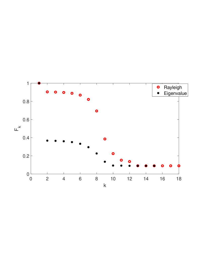
Fig. 7.1: Behaviour of the algorithm based on the Rayleigh quotient (circles) versus the algorithm based on the eigenvalue computation (bullets).

We note that the final value of $\widetilde{F}_{\varepsilon}(v)\approx 0.08976$; the difference with respect to the corresponding approximation computed by the method making use of eigenvalues is roughly $5\times 10^{-7}$ implying an error on the sixth significant digit. The number of steps executed by the numerical integrator is comparable ($18$ for the Rayleigh quotient and $15$ for the eigenvalue method). The structured dissipativity radius of $A=-I$ is approximately computed as $\varepsilon_{\star}\approx 1.098614111289907$, whereas the unstructured dissipativity radius equals 1.

$k$	$\varepsilon_{k}$	$-\omega(A+\varepsilon_{k}E(\varepsilon_{k}))$	$\#$ Rayleigh
​​​​ $0$	$1$	$1.856586036644719$	$18$
$1$	$1.098615122565759$	$0.920501421999773\cdot 10^{-6}$	$13$
$2$	$1.098614111289907$	$6.104818325601980\cdot 10^{-12}$	$10$

Table 7.1: Computation of the dissipativity radius: computed values $\varepsilon_{k}$, $-\omega(A+\varepsilon_{k}E(\varepsilon_{k}))$ and number of Rayleigh quotient computations of the inner algorithm.

V.8 Structured distance to singularity

Let $A\in\mathbb{C}^{n,n}$ be an invertible matrix, and let $\mathcal{S}$ be a complex- or real-linear subspace of $\mathbb{C}^{n,n}$ that defines the linear structure that is imposed on perturbations $\Delta\in\mathcal{S}$ to $A$. We consider the following structured matrix nearness problem.

Problem. Given an invertible matrix $A$, find a structured perturbation $\Delta\in\mathcal{S}$ of minimal Frobenius norm such that $A+\Delta$ is singular.

The norm of the minimizing $\Delta\in\mathcal{S}$ is called the $\mathcal{S}$-structured distance to singularity of the given matrix $A$. Unlike the complex or real unstructured distance to singularity, the $\mathcal{S}$-structured distance to singularity (for $\mathcal{S}\neq\mathbb{C}^{n,n},\mathbb{R}^{n,n}$) cannot be obtained from a singular value decomposition of $A$.

An obvious case of interest is when $\mathcal{S}$ is a space of complex or real matrices with a prescribed sparsity pattern. At the end of this section we consider a different situation where a structured distance to singularity is of interest: Given two polynomials, compute the nearest pair of polynomials with a common zero. This can be rephrased as the above problem with $\mathcal{S}$ the space of Sylvester matrices.

V.8.1 Optimizing eigenvalues or singular values

For the computation of the structured distance to singularity we can use the two-level iteration of Section IV.1. In the inner iteration we could again do eigenvalue optimization using the rank-1 algorithm of Section V.2 with $f(\lambda,\overline{\lambda})=\lambda\overline{\lambda}=|\lambda|^{2}$, choosing the eigenvalue of smallest modulus as the target eigenvalue (the smallest singular value could be used in an alternative algorithm). We note that here the structured gradient is $G_{\varepsilon}^{\mathcal{S}}(E)=\Pi^{\mathcal{S}}(\lambda xy^{*})$, for the (simple) eigenvalue $\lambda=\lambda(A+\varepsilon E)$ with left and right eigenvectors $x$ and $y$ of norm 1 and with positive inner product. Alternatively, the smallest singular value could be minimized under structured perturbations of Frobenius norm $\varepsilon$. The outer iteration for finding the minimal $\varepsilon$ yielding a zero eigenvalue or singular value uses the Newton–bisection method described in Section IV.1.5.

V.8.2 Optimizing norms of matrix–vector products

We now turn to a different approach that requires only matrix–vector products instead of computations of eigenvalues and eigenvectors or singular values and singular vectors. To avoid some technical complications that would obscure the basic argument, we consider in this subsection the real case:

$$A\in\mathbb{R}^{n,n} \mathcal{S}\subset\mathbb{R}^{n,n}$$ is a real matrix and is a real structure space.

In an approach that does not require the computation of eigenvalues and eigenvectors (or singular values and singular vectors) in every iteration, we first consider the following functional, which only contains the Euclidean norms of matrix–vector products:

$$F_{\varepsilon}(E,u,v)=\tfrac{1}{2}\,\|u^{\top}(A+\varepsilon E)\|^{2}+\tfrac{1}{2}\,\|(A+\varepsilon E)v\|^{2}$$ (8.1)

is to be minimized over all $E\in\mathcal{S}$ of Frobenius norm 1 and all $u,v\in\mathbb{R}^{n}$ of Euclidean norm 1.

It will turn out that in a minimum, $u$ and $v$ are left and right singular vectors of $A+\varepsilon E$, and $E=-\Pi^{\mathcal{S}}(uv^{\top})/\|\Pi^{\mathcal{S}}(uv^{\top})\|$. We will then restrict the functional $F_{\varepsilon}$ to such $E$, obtaining a functional of two vectors $u$ and $v$ only. This reduced functional $\widetilde{F}_{\varepsilon}(u,v)$ will be used in the two-level approach, minimizing $\widetilde{F}_{\varepsilon}$ for a fixed $\varepsilon$ in the inner iteration and determining the smallest $\varepsilon$ with $\widetilde{F}_{\varepsilon}(u(\varepsilon),v(\varepsilon))=0$ in the outer iteration. We closely follow the programme of Section V.7.3.

Structured gradient.

Consider a smooth path of structured matrices $E(t)\in\mathcal{S}$ and vectors $u(t),v(t)\in\mathbb{C}^{n}$. Since then also $\dot{E}(t)\in\mathcal{S}$, we have

$$\frac{d}{dt}\,F_{\varepsilon}(E(t),u(t),v(t))$$

$$=\,\langle u^{\top}(A+\varepsilon E),\varepsilon u^{\top}\dot{E}+\dot{u}^{\top}(A+\varepsilon E)\rangle+\,\langle(A+\varepsilon E)v,\varepsilon\dot{E}v+(A+\varepsilon E)\dot{v}\rangle$$

$$=\varepsilon\,\langle G,\dot{E}\rangle+\,\langle(A+\varepsilon E)(A+\varepsilon E)^{\top}u,\dot{u}\rangle+\,\langle(A+\varepsilon E)^{\top}(A+\varepsilon E)v,\dot{v}\rangle$$ (8.2)

with the structured gradient matrix

$$G=G_{\varepsilon}^{\mathcal{S}}(E,u,v)=\Pi^{\mathcal{S}}\bigl{(}uu^{\top}(A+\varepsilon E)+(A+\varepsilon E)vv^{\top}\bigr{)},$$

which is the projection onto $\mathcal{S}$ of a matrix of rank at most 2.

Norm- and structure-constrained gradient flow.

Taking the norm constraints into account, we arrive at the following system of differential equations:

$$\varepsilon\dot{E} =-G+\,\langle G,E\rangle\,E$$

$$\alpha\,\dot{u} =-(A+\varepsilon E)(A+\varepsilon E)^{\top}u+\|(A+\varepsilon E)^{\top}u\|^{2}\,u$$ (8.3)

$$\beta\,\dot{v} =-(A+\varepsilon E)^{\top}(A+\varepsilon E)v+\|(A+\varepsilon E)v\|^{2}\,v,$$

with scaling factors $\alpha(t)>0$ and $\beta(t)>0$, which we propose to choose as $\alpha=\|(A+\varepsilon E)^{\top}u\|$ and $\beta=\|(A+\varepsilon E)v\|$ to obtain similar rates of change in $\varepsilon E$, $u$, $v$ near a stationary point.

By construction, the Frobenius norm 1 of $E(t)$ and the Euclidean norm 1 of $u(t)$ and $v(t)$ are preserved, and the functional $F_{\varepsilon}$ decays monotonically along solutions.

Stationary points.

At stationary points $(E,u,v)$ we find that $u$ and $v$ are eigenvectors to the same positive eigenvalue $\sigma^{2}$ of $(A+\varepsilon E)(A+\varepsilon E)^{\top}$ and $(A+\varepsilon E)^{\top}(A+\varepsilon E)$, respectively. If the sign of $u$ is such that $u^{\top}(A+\varepsilon E)v$ is real and positive, then $u$ and $v$ are left and right singular vectors of $A+\varepsilon E$ to the singular value $\sigma>0$. We then have $\sigma u=(A+\varepsilon E)v$ and $\sigma v=(A+\varepsilon E)^{\top}u$ and hence $G=\Pi^{\mathcal{S}}(2\sigma uv^{\top})$ in the stationary point. If $G\neq 0$, it follows that $E$ is a multiple of $\Pi^{\mathcal{S}}(uv^{\top})$.

• (Non-vanishing gradient). If $A\in\mathcal{S}$ and $\sigma\neq 0$, then $G\neq 0$.

  • The proof uses a similar argument to the proof of Theorem V.2.3. We have

    $$\langle G,A+\varepsilon E\rangle=2\sigma\langle\Pi^{\mathcal{S}}(uv^{\top}),A+\varepsilon E\rangle$$

    $$=2\sigma\langle uv^{\top},\Pi^{\mathcal{S}}(A+\varepsilon E)\rangle=2\sigma\langle uv^{\top},A+\varepsilon E\rangle$$

    $$=2\sigma\langle u,(A+\varepsilon E)v\rangle=2\sigma\langle u,\sigma u\rangle=2\sigma^{2}\neq 0,$$

    and hence $G\neq 0$.   $\sqcap$$\sqcup$

    Moreover, if the equality constraint for the Frobenius norm $1$ is replaced by an inequality constraint $\leq 1$, then the same argument as in the proof of Theorem II.6.5 shows that $E$ is a negative multiple of $\Pi^{\mathcal{S}}(uv^{\top})$ and still has norm 1, so that

    $$E=-\frac{\Pi^{\mathcal{S}}(uv^{\top})}{\|\Pi^{\mathcal{S}}(uv^{\top})\|_{F}}.$$ (8.4)

    These findings lead us to the following theorem.

    • (Optimal perturbation).  Let $A\in\mathcal{S}$ be invertible. Then, there exists a perturbation $\Delta\in\mathcal{S}$ of minimal Frobenius norm with singular $A+\Delta$, which is the orthogonal projection of a rank-1 matrix onto $\mathcal{S}$. In more detail, $\Delta$ is a negative multiple of $\Pi^{\mathcal{S}}(uv^{\top})$, where $u$ and $v$ are left and right singular vectors to a singular value $0$ of $A+\Delta$.

      • The proof combines the above results for $\varepsilon<\varepsilon_{\star}$ with a compactness argument as $\varepsilon\nearrow\varepsilon_{\star}$. For every $\varepsilon<\varepsilon_{\star}$ we have $\sigma_{\min}(A+\varepsilon E(\varepsilon))\neq 0$, and hence $\varepsilon E(\varepsilon)$ is of the stated form (8.4). By the Bolzano–Weierstraß theorem, there exists a subsequence $(\varepsilon_{n})$ with $\varepsilon_{n}\nearrow\varepsilon_{\star}$ such that the corresponding $E(\varepsilon_{n})$, $u(\varepsilon_{n})$ and $v(\varepsilon_{n})$ converge. This implies the result.   $\sqcap$$\sqcup$

Reduced functional.

We insert (8.4) into the functional (8.1) and minimize the resulting reduced functional of two vectors $u,v\in\mathbb{C}^{n}$ of norm 1 only:

$$\widetilde{F}_{\varepsilon}(u,v)=\tfrac{1}{2}\,\|u^{\top}(A+\varepsilon E)\|^{2}+\tfrac{1}{2}\,\|(A+\varepsilon E)v\|^{2}\quad\text{ with }\ E=-\frac{\Pi^{\mathcal{S}}(uv^{\top})}{\|\Pi^{\mathcal{S}}(uv^{\top})\|_{F}}.$$

Here we assume that the signs of $u$ and $v$ are such that $u^{\top}(A+\varepsilon E)v>0$. We will not discuss exceptional situations where this term becomes zero or where the denominator in the expression for $E$ becomes zero.

• (Reduced gradient).  Along a path $(u(t),v(t))\in\mathbb{R}^{n}\times\mathbb{R}^{n}$, we have (omitting the argument $t$)

  $$\frac{d}{dt}\,\widetilde{F}_{\varepsilon}(u(t),v(t))=\langle g,\dot{u}\rangle+\langle h,\dot{v}\rangle$$

  with

  $$g =(A+\varepsilon E)(A+\varepsilon E)^{\top}u-\varepsilon\eta^{2}\gamma Ev-\varepsilon\eta Gv$$

  $$h =(A+\varepsilon E)^{\top}(A+\varepsilon E)v-\varepsilon\eta^{2}\gamma E^{\top}u-\varepsilon\eta G^{\top}u,$$

  where $E=-\eta\Pi^{\mathcal{S}}(uv^{\top})$ and $\eta=1/\|\Pi^{\mathcal{S}}(uv^{\top})\|_{F}$, and
  $G=\Pi^{\mathcal{S}}\bigl{(}uu^{\top}(A+\varepsilon E)+(A+\varepsilon E)vv^{\top}\bigr{)}$ and $\gamma=u^{\top}Gv$.

  • We have

    $$\dot{E} =-\dot{\eta}\,\Pi^{\mathcal{S}}(uv^{\top})-\eta\,\Pi^{\mathcal{S}}(\dot{u}v^{\top}+u\dot{v}^{\top})\quad\text{with }$$

    $$\dot{\eta} =-\eta^{3}\langle\Pi^{\mathcal{S}}(uv^{\top}),\dot{u}v^{\top}+u\dot{v}^{\top}\rangle=\eta^{2}\langle Ev,\dot{u}\rangle+\eta^{2}\langle E^{\top}u,\dot{v}\rangle.$$

    This yields, using that $G\in\mathcal{S}$,

    $$\langle G,\dot{E}\rangle =\eta^{3}\langle\Pi^{\mathcal{S}}(uv^{\top}),\dot{u}v^{\top}+u\dot{v}^{\top}\rangle\,\gamma-\eta\langle G,\dot{u}v^{\top}+u\dot{v}^{\top}\rangle$$

    $$=\langle-\eta^{2}\gamma Ev-\eta Gv,\dot{u}\rangle+\langle-\eta^{2}\gamma E^{\top}u-\eta G^{\top}u,\dot{v}\rangle.$$

    Inserting this expression into (8.2) yields the stated result.   $\sqcap$$\sqcup$

Norm-constrained reduced gradient flow.

In view of Lemma V.8.2, the norm-constrained gradient flow of the reduced functional takes the form

$$\begin{array}[]{rcl}\dot{u}&=&-g+\langle g,u\rangle u\\[2.84526pt] \dot{v}&=&-h+\langle h,v\rangle v.\end{array}$$ (8.5)

The Euclidean norm 1 of $u(t)$ and $v(t)$ is preserved for all $t$, and the reduced functional $\widetilde{F}_{\varepsilon}$ decays monotonically along solutions of this differential equation.

We numerically integrate the differential equation (8.5) for the two vectors $u(t)$ and $v(t)$ into a stationary point. In each time step, this algorithm just requires computing matrix–vector products and inner products of vectors but no computations of eigenvalues and eigenvectors or singular values and singular vectors. The sign of $u$ in the initial value is chosen such that $u^{\top}(A+\varepsilon E)v>0$, and this sign condition is monitored over the discrete trajectories.

In this way we aim to determine

$$(u(\varepsilon),v(\varepsilon))=\arg\min_{u,v}\;\widetilde{F}_{\varepsilon}(u,v)\quad\text{and}\quad E(\varepsilon)=-\frac{\Pi^{\mathcal{S}}(u(\varepsilon)v(\varepsilon)^{\top})}{\|\Pi^{\mathcal{S}}(u(\varepsilon)v(\varepsilon)^{\top})\|_{F}},$$

where the minimum is taken over all $u,v\in\mathbb{R}^{n}$ of Euclidean norm 1.

• (Complex case). The approach taken here extends to the complex case, where the phase of $u$ is chosen such that $u^{*}(A+\varepsilon E)v$ is real and positive. This can be ensured by adding the constraint ${\mbox{\rm Im}}(u^{*}(A+\varepsilon E)v)=0$ via an extra term $\mathrm{i}\omega u$ to the differential equation for $u$, where $\omega$ is determined such that the time-differentiated constraint is satisfied. Note that the functional is invariant under rotations ${\rm e}^{\mathrm{i}\theta}u$.

Outer iteration.

The optimal perturbation size ${\varepsilon_{\star}}$ is determined as the smallest $\varepsilon>0$ such that for a given tolerance $\vartheta\ll 1$,

$$\sigma_{\min}(A+\varepsilon E(\varepsilon))=\Bigl{(}\tfrac{1}{2}\,\|u(\varepsilon)^{\top}(A+\varepsilon E(\varepsilon))\|^{2}+\tfrac{1}{2}\,\|(A+\varepsilon E(\varepsilon))v(\varepsilon)\|^{2}\Bigr{)}^{1/2}\leq\vartheta\,\|A\|_{2}.$$

Here the first equality holds true because $u(\varepsilon)$ and $v(\varepsilon)$ are left and right singular vectors associated with the smallest singular value of $A+\varepsilon E(\varepsilon)$. This scalar equation (up to $O(\theta))$ is again solved by a Newton–bisection algorithm. Here we use the following simple expression for the derivative.

• We have

  $$\frac{d}{d\varepsilon}\sigma_{\min}(A+\varepsilon E(\varepsilon))=-\|\Pi^{\mathcal{S}}(u(\varepsilon)v(\varepsilon)^{\top})\|_{F}.$$

  • By Corollary IX.IX.1,

    $$\frac{d}{d\varepsilon}\sigma_{\min}(A+\varepsilon E(\varepsilon))=u(\varepsilon)^{\top}\bigl{(}E(\varepsilon)+\varepsilon E^{\prime}(\varepsilon)\bigr{)}v(\varepsilon).$$

    We find

    $$u(\varepsilon)^{\top}E^{\prime}(\varepsilon)v(\varepsilon) =\langle u(\varepsilon)v(\varepsilon)^{\top},E^{\prime}(\varepsilon)\rangle=\langle\Pi^{\mathcal{S}}(u(\varepsilon)v(\varepsilon)^{\top}),E^{\prime}(\varepsilon)\rangle$$

    $$=-\mu\langle E(\varepsilon),E^{\prime}(\varepsilon)\rangle=-\frac{\mu}{2}\frac{d}{d\varepsilon}\|E(\varepsilon)\|_{F}^{2}=0$$

    with the irrelevant factor $\mu=\|\Pi^{\mathcal{S}}(u(\varepsilon)v(\varepsilon)^{\top})\|_{F}$. So we have

    $$\frac{d}{d\varepsilon}\sigma_{\min}(A+\varepsilon E(\varepsilon))=u(\varepsilon)^{\top}E(\varepsilon)v(\varepsilon)=-u(\varepsilon)^{\top}\frac{\Pi^{\mathcal{S}}(u(\varepsilon)v(\varepsilon)^{\top})}{\|\Pi^{\mathcal{S}}(u(\varepsilon)v(\varepsilon)^{\top})\|_{F}}\,v(\varepsilon)$$

    $$=-\frac{\langle u(\varepsilon)v(\varepsilon)^{\top},\Pi^{\mathcal{S}}(u(\varepsilon)v(\varepsilon)^{\top})}{\|\Pi^{\mathcal{S}}(u(\varepsilon)v(\varepsilon)^{\top})\|_{F}}=-\frac{\langle\Pi^{\mathcal{S}}(u(\varepsilon)v(\varepsilon)^{\top}),\Pi^{\mathcal{S}}(u(\varepsilon)v(\varepsilon)^{\top})\rangle}{\|\Pi^{\mathcal{S}}(u(\varepsilon)v(\varepsilon)^{\top})\|_{F}}$$

    $$=-\|\Pi^{\mathcal{S}}(u(\varepsilon)v(\varepsilon)^{\top})\|_{F}$$

    as stated in the lemma.   $\sqcap$$\sqcup$

V.8.3 Example: Nearest pair of polynomials with a common zero

We consider polynomials with real coefficients (alternatively, we could allow for complex coefficients). A pair of polynomials $(p,q)$ is called coprime if $p$ and $q$ have no nontrivial common divisor, or equivalently, have no common zero. For a pair of polynomials $(p,q)$ that is coprime, the distance to the nearest pair of polynomials with a common zero is of interest. In the following we measure the distance of pairs of polynomials by the Euclidean norm of the difference of the vectors of coefficients in the monomial basis.

Problem. Given a pair of polynomials that is coprime, find the nearest pair of polynomials with a nontrivial common divisor.

Consider polynomials

$$\begin{array}[]{rcl}p(z)&=&a_{n}z^{n}+a_{n-1}z^{n-1}+\cdots+a_{1}z+a_{0}\\[5.69054pt] q(z)&=&b_{m}z^{m}+b_{m-1}z^{m-1}+\cdots+b_{1}z+b_{0}\end{array}$$ (8.8)

with real coefficients $a_{i}$ and $b_{i}$. We may assume $m\leq n$ and $a_{n}\neq 0$, and we can take $m=n$ if we allow for $b_{n}=0$. So we assume $m=n$ in the following. With these polynomials we associate the Sylvester matrix of dimension $2n\times 2n$,

$$S(p,q):=\begin{pmatrix}a_{n}&&\ldots&&a_{0}&&&\\ &a_{n}&&\ldots&&a_{0}&&\\ &&\ddots&&&&\ddots&\\ &&&a_{n}&&\ldots&&a_{0}\\ b_{n}&&\ldots&&b_{0}&&&\\ &b_{n}&&\ldots&&b_{0}&&\\ &&\ddots&&&&\ddots&\\ &&&b_{n}&&\ldots&&b_{0}\end{pmatrix}.$$ (8.9)

A result from commutative algebra (see Laidacker (?)) states:
The pair of polynomials $(p,q)$ is coprime if and only if the associated Sylvester matrix $S(p,q)$ is invertible.

This allows us to reformulate the problem of nearest non-coprime polynomials as a matrix nearness problem, where the distance is measured by the Frobenius norm.

Problem. Given an invertible Sylvester matrix, find the nearest singular Sylvester matrix.

This amounts to the problem of computing the structured distance to singularity, where the structure is given by the subspace $\mathcal{S}\subset\mathbb{R}^{2n,2n}$ of Sylvester matrices of the form (8.9).

Let $S$ be a Sylvester matrix. We define the lower radius of $S$ as

$$\mu(S)=\min\{|\lambda|\,:\,\lambda\text{ is an eigenvalue of S}\},$$

and note that $S$ is singular if and only if $\mu(S)=0$. Furthermore, with the structured $\varepsilon$-pseudospectrum $\Lambda_{\varepsilon}^{\mathcal{S}}(S)$, let

$$\mu_{\varepsilon}^{\mathcal{S}}(S)=\min\{|\lambda|:\lambda\in\Lambda_{\varepsilon}^{\mathcal{S}}(S)\},$$ (8.10)

which reduces to the lower radius $\mu(S)$ when $\varepsilon=0$. We can then express the radius of coprimeness of the pair of polynomials $(p,q)$ as

$$\rho_{\rm co}(p,q)=\frac{\varepsilon_{\star}}{\sqrt{n}}\quad\text{ with }\quad\varepsilon_{\star}=\min\{\varepsilon>0\,:\,\mu_{\varepsilon}^{\mathcal{S}}(S)=0\}.$$

(The division by $\sqrt{n}$ is done to account for the fact that each coefficient $a_{i}$ and $b_{i}$ appears $n$ times in the Sylvester matrix, which yields a factor $\sqrt{n}$ in the Frobenius norm.)

Two-level iteration.

We are thus in the situation of applying the two-level iteration of Section IV.1 with the functional $F_{\varepsilon}(E)$ (for $E\in\mathcal{S}$ of unit Frobenius norm) given as

$$F_{\varepsilon}(E)=\mu(S+\varepsilon E),$$ (8.11)

which is of the form (1.3) with $f(\lambda,\overline{\lambda})=\sqrt{\lambda\overline{\lambda}}$ and with the eigenvalue of smallest modulus as target eigenvalue.

To apply the gradient-based algorithm of Section V.2 in the inner iteration, we need the structured gradient, see II.2.4), which is the orthogonal projection onto the space $\mathcal{S}$ of Sylvester matrices of the (rescaled) gradient

$$G_{\varepsilon}(E)={\mbox{\rm Re}}\Bigl{(}\frac{\lambda}{|\lambda|}\,xy^{*}\Bigr{)},$$

where $x$ and $y$ are the left and right eigenvectors, normalized to unit norm and with positive inner product, that are associated with the eigenvalue $\lambda$ of smallest modulus of $S+\varepsilon E$, which is assumed to be simple. We note that the structured gradient is nonzero by Theorem V.2.3.

The orthogonal projection onto $\mathcal{S}$ is given in the following lemma.

• (Orthogonal projection onto the space of Sylvester matrices).  Let $S\in\mathcal{S}\subset\mathbb{R}^{2n\times 2n}$ and $Z\in\mathbb{C}^{2n,2n}$; the orthogonal projection $P_{\mathcal{S}}$ onto $\mathcal{S}$, with respect to the Frobenius inner product $\langle\cdot,\cdot\rangle$, is given by

  $$\Pi^{\mathcal{S}}Z = S(p,q),$$ (8.12)

  where $p$ and $q$ are the polynomials with coefficients (for $k=0,\ldots,n$)

  $$a_{n-k}=\frac{1}{n}\sum\limits_{l=1}^{n}{\mbox{\rm Re}}\left(Z_{l,l+k}\right),\qquad b_{n-k}=\frac{1}{n}\sum\limits_{l=1}^{n}{\mbox{\rm Re}}\left(Z_{n+l,l+k}\right).$$

  • We have to find $\arg\min_{S\in\mathcal{S}}\|Z-S\|_{F}$. The result follows directly from the fact that for a complex vector $x\in\mathbb{C}^{n}$,

    $$\mu_{*}=\arg\min\limits_{\mu\in\mathbb{R}}\|x-\mu 1\kern-2.23999pt\hbox{\rm l}\|_{F}=\frac{1}{n}\sum\limits_{i=1}^{n}{\mbox{\rm Re}}(x_{i}),$$

    where $1\kern-2.23999pt\hbox{\rm l}=\left(1\ 1\ \ldots\ 1\right)^{\top}$.   $\sqcap$$\sqcup$

Numerical example.

Consider the two polynomials of degree $3$,

$$p(z)=z^{3}+2z^{2}+2z+2,\quad\ q(z)=2z^{3}+z-2,$$ (8.13)

where $p$ is constrained to be monic. Here $a=\left(1\ 1\ 2\ 2\right)^{\top}$ and $b=\left(2\ 0\ 1\ -2\right)^{\top}$; the corresponding Sylvester matrix is given by

$$S(a,b)=\left(\begin{array}[]{rrrrrr}1&2&2&2&0&0\\ 0&1&2&2&2&0\\ 0&0&1&2&2&2\\ 2&0&1&-2&0&0\\ 0&2&0&1&-2&0\\ 0&0&2&0&1&-2\end{array}\right)$$ (8.14)

The structured pseudospectrum $\Lambda_{\varepsilon}^{\mathcal{S}}(S)$ for $\varepsilon=\frac{1}{2}$ is approximated by dense sampling on the set of admissible perturbations and is plotted in blue in Figure 8.1.

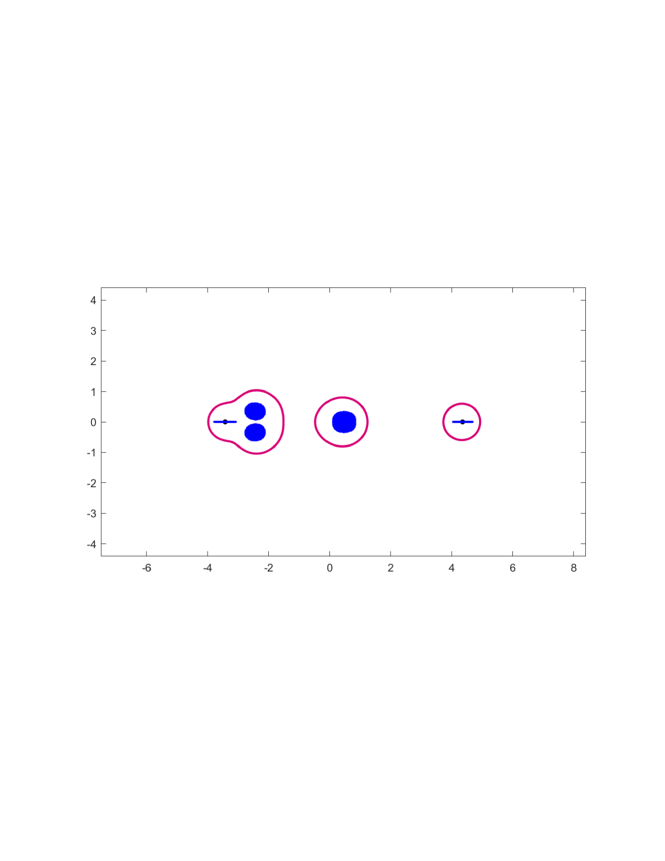
Fig. 8.1: The approximated structured Sylvester $\varepsilon$-pseudospectrum for $\varepsilon=\frac{1}{2}$ for Example (8.14) is filled with blue. The red curve represents the boundary of the set of eigenvalues obtained by considering arbitrary complex perturbations (that is omitting the constraint of real Sylvester structure) of norm bounded by $\frac{1}{2}$.

It turns out that for the value

$$\varepsilon=\varepsilon_{\star}=0.618108064$$

the functional $F_{\varepsilon}(E)$ (see (8.11)) vanishes, while for $\varepsilon<\varepsilon_{\star}$ it holds $F_{\varepsilon}(E)>0$. This gives $\rho_{\rm co}(p,q)=0.356864857$.

The computed matrix $S+\varepsilon_{\star}E(\varepsilon_{\star})$ has rank $2n-2$ due to a double semi-simple zero eigenvalue. The coefficients of the perturbed polynomials $\hat{p}$, $\hat{q}$ are shown (with $10$-digit accuracy) in Table 8.1. The common complex conjugate zeros of $\hat{p}$, $\hat{q}$ are

$$z_{1,2}=-0.4008686595\pm 1.03085391659\mathrm{i}.$$

Table 8.1: Coefficients of the perturbed polynomials $\hat{p}$, $\hat{q}$ in the example 8.13.

$\begin{array}[]{llllll}\hat{a}_{3}=0.75744188&\hat{a}_{2}=2.10479150&\hat{a}_{1}=2.12724001&\hat{a}_{0}=1.83200184\\[2.84526pt] \hat{b}_{3}=1.95430087&\hat{b}_{2}=-0.06706025&\hat{b}_{1}=1.08084913&\hat{b}_{0}=-1.99883585\end{array}$

V.9 Notes

Low-rank matrix differential equations for structured eigenvalue optimization.

The approach to structured eigenvalue optimization via a norm-constrained gradient system and the associated low-rank dynamics was first proposed and studied by Guglielmi & Lubich (?), where rank-2 differential equations were used to compute the real $\varepsilon$-pseudospectral abscissa and radius. Guglielmi, Kressner & Lubich (?) studied Hamiltonian eigenvalue optimization using rank-4 matrix differential equations; see also Section VI.2. The structure-projected rank-1 approach in Section V.2 to eigenvalue optimization with general linear structures $\mathcal{S}$ was developed by Guglielmi, Lubich & Sicilia (?).

Our discussion of low-rank dynamics in Sections II.3.3 and V.1.4 is based on Koch & Lubich (?). Numerical integrators for low-rank matrix differential equations that are robust to small singular values are given by the projector-splitting integrator of Lubich & Oseledets (?) and the basis-update & Galerkin (BUG) integrator of Ceruti & Lubich (?), of which a norm-preserving variant is presented in Section V.1.5.

Frobenius norm vs. matrix 2-norm.

In the real case and structured cases, where the Frobenius-norm and matrix 2-norm optimizers are in general different, functional-reducing differential equations for the 2-norm constrained eigenvalue optimization problem have been given that have similar properties to the gradient systems for the Frobenius-norm problem considered here; see Guglielmi & Lubich (?) for the computation of the 2-norm real pseudospectral abscissa and Guglielmi, Kressner & Lubich (?) for 2-norm constrained eigenvalue optimization problems for Hamiltonian matrices.

Graillat (?) and Rump (?) proved that for complex Toeplitz and Hankel structures, the 2-norm structured pseudospectrum equals the unstructured pseudospectrum. This is not valid in the Frobenius norm, and it is not valid for real Toeplitz and Hankel matrices.

Computing structured pseudospectra.

The approach of Karow, Kokiopoulou and Kressner (?) to compute structured pseudospectra w.r.t. the matrix 2-norm uses structured singular values $\mu^{\mathcal{S}}(B)=(\inf\{\|\Delta\|_{2}\,:\,\Delta\in\mathcal{S}\text{ and $I-\Delta B$ is a singular matrix}\})^{-1},$ which yield the characterization $\Lambda_{\varepsilon}^{\mathcal{S}}(A)=\{\lambda\in\mathbb{C}\,:\,\mu^{\mathcal{S}}\bigl{(}(A-\lambda I)^{-1}\bigr{)}\geq 1/\varepsilon\}.$ Note that $1/\mu^{\mathcal{S}}\bigl{(}(A-\lambda I)^{-1}\bigr{)}$ equals the structured 2-norm distance to singularity of $A-\lambda I$; cf. Section V.8, where the structured Frobenius-norm distance to singularity is considered. For the unstructured complex case we have $\mu^{\mathbb{C}}(B)=\|B\|_{2}$, and for the unstructured real case, an expression for $\mu^{\mathbb{R}}(B)$ was given by Qiu et al. (?). Based on that result, Karow, Kokiopoulou and Kressner (?) gave an algorithm to compute real pseudospectra. They also found expressions for structured singular values for complex skew-symmetric, Hermitian and complex Hamiltonian matrices, which allowed them to extend their algorithm to these particular structures. For the Frobenius-norm structured pseudospectrum, their basic algorithm can be combined with the algorithm for the structured distance to singularity of Section V.8 to compute the Frobenius-norm structured singular values of the resolvents $(A-\lambda I)^{-1}$ for general linear structures.

Buttà, Guglielmi & Noschese (?) proposed an algorithm to compute the structured $\varepsilon$-pseudospectral abscissa (w.r.t. the Frobenius norm) and sections of the boundary of structured pseudospectra for complex Toeplitz matrices. This algorithm is related to the rank-1 iteration of Guglielmi & Overton (?).

The ladder algorithm and its structured version used in Section V.3.3, which traces sections of the boundary of structured pseudospectra (w.r.t. the Frobenius norm) for arbitrary linear structures $\mathcal{S}$, have not previously appeared in the literature.

Stability radius under real unstructured perturbations.

Qiu, Bernhardsson, Rantzer, Davison, Young & Doyle (?) characterized the real stability radius $r_{\mathbb{R}}(A)$ as

$$\frac{1}{r_{\mathbb{R}}(A)}=\sup_{\omega\in\mathbb{R}}\inf_{0<\gamma\leq 1}\sigma_{2}\begin{pmatrix}{\mbox{\rm Re}}\,M_{\omega}&-\gamma\,{\mbox{\rm Im}}\,M_{\omega}\\ \gamma^{-1}{\mbox{\rm Im}}\,M_{\omega}&{\mbox{\rm Re}}\,M_{\omega}\end{pmatrix}\quad\ \text{with}\quad M_{\omega}=(A-\mathrm{i}\omega I)^{-1},$$

where $\sigma_{2}(\cdot)$ is the second largest singular value of a matrix. An algorithm for the computation of $r_{\mathbb{R}}(A)$ via this formula was proposed by Sreedhar, Van Dooren & Tits (?). Based on a reformulation of this formula and using Byers’ connection between singular values and eigenvalues of Hamiltonian matrices, Freitag & Spence (?) also developed an algorithm to deal efficiently with this two-dimensional optimization.

In a different approach, Lu & Vandereycken (?) developed a criss-cross-type algorithm (cf. III.2) for computing the real pseudospectral abscissa.

Guglielmi & Manetta (?) studied an algorithm that is well-suited also for large sparse matrices. It corresponds to the general two-level approach taken in Section IV.1. In the inner iteration, the algorithm computes the real $\varepsilon$-pseudospectral abscissa via rank-2 matrix differential equations of Guglielmi & Lubich (?) (which are given there for both the matrix 2-norm and the Frobenius norm). In the outer iteration, it uses a combined Newton–bisection method to optimize the perturbation size $\varepsilon$ to yield $\varepsilon_{\star}$ such that the real $\varepsilon_{\star}$-pseudospectral abscissa becomes zero. The Newton iteration used the simple derivative formula of Theorem IV.1.4 for the particular case of the real gradient $G={\mbox{\rm Re}}(xy^{*})$. A related method based on a real version of the iteration method of Guglielmi & Overton (?) was proposed by Rostami (?) and further developed and analysed by Guglielmi (?).

Structured stability radii.

In the control systems literature, Hinrichsen & Pritchard (?,?,?) considered complex and real stability radii (i.e. distance to instability under complex and real perturbations) and also structured stability radii

$$r(A,B,C)=\min\{\|\Delta\|\,:\,A+B\Delta C\text{ has some eigenvalue of nonnegative real part}\},$$

where $A$ is a Hurwitz-stable matrix and $B$ and $C$ are given matrices of compatible dimensions. The perturbation matrix $\Delta$ is assumed to be real or complex. Most of the algorithms mentioned above extend to this situation of range- and corange-restricted perturbations. For example, Hinrichsen, Kelb & Linnemann (?) extended Byers’ algorithm to compute the complex structured stability radius $r_{\mathbb{C}}(A,B,C)$.

We note that this notion of structured stability radius minimizes the norm of the parameter matrix $\Delta$ and not of the structured perturbation $B\Delta C$ of $A$. The latter would fit directly into the framework of Section IV.1, whereas controlling the norm of $\Delta$ requires some (minor) modifications to the algorithm.

We are not aware of algorithms for other structured stability radii (distance to instability under complex or real structured perturbations) in the literature, e.g. for perturbations with a given sparsity pattern and/or symmetry, or Toeplitz perturbations etc. The two-level algorithm of Section IV.1 addresses such problems with general linear structures.

Transient bounds under structured perturbations.

The joint unstructured–structured pseudospectrum and the structured $\varepsilon$-stability radius were introduced by Guglielmi & Lubich (?) as basic notions to assess the robustness of transient bounds of linear dynamical systems under structured perturbations of the matrix. The rank-1 algorithm of Section V.6 for computing the structured $\varepsilon$-stability radius was also proposed and studied there.

Numerical range under structured perturbations.

The algorithm in Section V.7 for computing the structured dissipativity radius using Rayleigh quotients instead of eigenvalues has not been published before. More generally, replacing eigenvalues by Rayleigh quotients in real symmetric and complex Hermitian eigenvalue optimization appears to yield a computationally favourable approach.

Structured distance to singularity.

While the unstructured 2-norm and Frobenius-norm distance to singularity of a matrix equal its smallest singular value, we are not aware of an algorithm in the literature for computing the distance to singularity under structured perturbations. Minimizing the norm of matrix-vector products within a two-level approach as is done in Section V.8 appears to be new.

Chapter VI Matrix nearness problems of diverse kinds

In this chapter we discuss extensions of the two-level approach to matrix nearness problems of diverse types that are not covered by the framework of the previous chapters, be it because

• the functional in the associated eigenvalue optimization problem depends not only on one target eigenvalue but on a varying number of eigenvalues, as in the problem of computing the nearest stable matrix to a given unstable matrix; or

• the problem requires special attention to the structure, as in Hamiltonian matrix nearness problems; or

• the functional in the associated eigenvalue optimization problem depends on eigenvectors, as in the Wilkinson problem of computing the nearest matrix with defective eigenvalues, which amounts to computing the distance to singularity of the eigenvalue condition number; or

• the nearness problem deals with matrix pencils, as in the problem of finding the nearest matrix pencil that is singular or additionally has a common null-vector; or

• the underlying eigenvalue problems are nonlinear in the eigenvalues, as in computing the stability radius of linear delay differential equations; or

• the given problem is not itself a matrix nearness problem but is addressed by the same techniques, such as computing the Kreiss number that appears in the Kreiss matrix theorem (which leads to generalized eigenvalue problems similar to the preceding item).

These items are exemplary, not exhaustive. They form the sections of this chapter. The sections can be read independently of each other, but we give fewer details in the later sections.

This chapter illustrates the versatility of the two-level approach that uses rank-constrained gradient flows in the inner iteration and combined Newton–bisection methods in the outer iteration. It enriches the toolbox for applications in various fields, such as those considered in the final chapters of this book. The proposed algorithms can deal with complex, real and structured perturbations.

VI.1 Matrix stabilization

In this section we extend the two-level approach of Chapter IV to the problem of moving all eigenvalues of a given matrix into a prescribed closed subset $\overline{\Omega}$ of the complex plane by a perturbation of minimal Frobenius norm. This spectral recovery problem is complementary to the robustness analysis in the previous two chapters where the original matrix has all its eigenvalues inside $\Omega$ and it was required that one eigenvalue be driven to the boundary of $\Omega$. While the approach presented here is conceptually applicable to the spectral recovery problem for very general subsets $\Omega$, we will focus our attention on the guiding problem of Hurwitz stabilization of an unstable matrix, which corresponds to the case where $\Omega={\mathbb{C}^{-}}$ is the left complex half-plane:

Problem. Given a square matrix $A$ that has some eigenvalues with positive real part, find a structured perturbation $\Delta\in\mathcal{S}$ of minimal Frobenius norm such that $A+\Delta$ has no eigenvalue with positive real part.

The perturbations $\Delta$ are restricted to lie in a structure space $\mathcal{S}$ that is $\mathbb{C}^{n,n}$ or $\mathbb{R}^{n,n}$ or a linear subspace thereof.

We describe two algorithmic approaches to this matrix stabilization problem, which are both of the two-level type considered in Chapter IV.

• The exterior algorithm moves eigenvalues that lie outside the closed target set $\overline{\Omega}$ where the eigenvalues of the perturbed matrix $A+\Delta$ should lie ($\overline{\Omega}=\overline{\mathbb{C}^{-}}$ for Hurwitz stability and $\overline{\Omega}$ is the closed unit disk for Schur stability). All eigenvalues outside $\overline{\Omega}$ are moved towards the boundary of $\Omega$ while increasing the perturbation size.

• The interior algorithm starts from a non-optimal perturbation $\Delta_{0}$ such that $A+\Delta_{0}$ has all eigenvalues in $\Omega$ and moves an eigenvalue inside $\Omega$ to the boundary while reducing the perturbation size.

VI.1.1 Exterior two-level algorithm

Here we use the following eigenvalue optimization problem: For a given perturbation size $\varepsilon>0$, find

$$\arg\min\limits_{\Delta\in\mathcal{S},\,\|\Delta\|_{F}=\varepsilon}\ \sum_{i=1}^{n}\,f\left(\lambda_{i}\left(A+\Delta\right),\overline{\lambda}_{i}\left(A+\Delta\right)\right),$$ (1.1)

with

$$f\left(\lambda,\overline{\lambda}\right)=\mbox{$\displaystyle{1\over 2}$}\,\text{dist}(\lambda,\overline{\mathbb{C}^{-}})^{2}=\mbox{$\displaystyle{1\over 2}$}\bigl{(}({\mbox{\rm Re}}\,\lambda)_{+}\bigr{)}^{2}=\mbox{$\displaystyle{1\over 8}$}\bigl{(}(\lambda+\overline{\lambda})_{+}\bigr{)}^{2},$$ (1.2)

where for $a\in\mathbb{R}$, $a_{+}:=\max\left\{a,0\right\}$.

The eigenvalues $\lambda_{i}(A+\Delta)$ ($i=1,\dots,n$) of the perturbed matrix $A+\Delta$ are ordered by decreasing size of the real part. Note that only the eigenvalues with positive real part contribute to the sum in (1.1), so that the sum only extends from 1 to $m^{+}(A+\Delta)$, where $m^{+}(M)$ is the number of eigenvalues of $M$ with positive real part. As in Chapter IV, this leads us to the following two-level approach to the Hurwitz stabilization problem. Here we additionally introduce a small shift $\delta>0$ that aims for strict Hurwitz stability with all eigenvalues having real part not exceeding $-\delta$.

• Inner iteration: Given $\varepsilon>0$, we aim to compute a matrix $E(\varepsilon)\in\mathcal{S}$ of unit Frobenius norm such that

  $$F_{\varepsilon}(E)=\mbox{$\displaystyle{1\over 2}$}\sum_{i=1}^{n}\,\bigl{(}({\mbox{\rm Re}}\,\lambda_{i}(A+\varepsilon E)+\delta)_{+}\bigr{)}^{2}$$ (1.3)

  is minimized, i.e.

  $$E(\varepsilon)=\arg\min\limits_{E\in\mathcal{S},\|E\|_{F}=1}F_{\varepsilon}(E).$$ (1.4)

• Outer iteration: We compute the smallest positive value $\varepsilon_{\star}$ with

  $$\phi(\varepsilon_{\star})=0,$$ (1.5)

  where $\phi(\varepsilon)=F_{\varepsilon}\left(E(\varepsilon)\right)=\tfrac{1}{2}\sum_{i=1}^{n}\,\bigl{(}({\mbox{\rm Re}}\,\lambda_{i}(A+\varepsilon E(\varepsilon)+\delta)_{+}\bigr{)}^{2}$.

We remark that the existence of a zero of $\phi$ (i.e., stabilizability) is not guaranteed for arbitrary structure spaces $\mathcal{S}$, but it is when $\mathcal{S}$ equals $\mathbb{C}^{n,n}$ or $\mathbb{R}^{n,n}$ or more generally when $\mathcal{S}$ contains real multiples of the identity matrix $I$ (since then some negative shift of the given matrix moves all its eigenvalues into the left half-plane).

As before, the inner iteration uses a norm- and structure-constrained gradient-flow differential equation, possibly further restricted to low-rank dynamics; the outer iteration uses a hybrid Newton–bisection method. We give details in the following subsections.

Constrained gradient flow for minimizing $F_{\varepsilon}(E)$

Here we let $\varepsilon>0$ be fixed. Let $E(t)\in\mathcal{S}$, for $t$ in an interval $I$, be a continuously differentiable path of matrices in the structure space $\mathcal{S}\subset\mathbb{C}^{n,n}$, and let the eigenvalues $\lambda_{i}(t)=\lambda_{i}(A+\varepsilon E(t))$ be simple for $i=1,\dots,n$ and all $t\in I$. The corresponding left and right eigenvectors $x_{i}$ and $y_{i}$ are assumed to be of unit norm and with $x_{i}^{*}y_{i}>0$. Then, applying Theorem IX.IX.1 we obtain

$$\frac{d}{dt}F_{\varepsilon}\bigl{(}E(t)\bigr{)}=\varepsilon\sum\limits_{i=1}^{n}\bigl{(}{\mbox{\rm Re}}\,\lambda_{i}(A+\varepsilon E(t))+\delta\bigr{)}_{+}\,\frac{{\mbox{\rm Re}}(x_{i}(t)^{*}\dot{E}(t)y_{i}(t))}{x_{i}(t)^{*}y_{i}(t)}.$$ (1.6)

We introduce the notation

$$\gamma_{i}(t):=\frac{\left({\mbox{\rm Re}}\,\lambda_{i}(A+\varepsilon E(t))+\delta\right)_{+}}{x_{i}(t)^{*}y_{i}(t)}\geq 0.$$

Here we note that $\gamma_{i}(t)=0$ for $i>m_{\delta}(A+\varepsilon E(t))$, which is the number of eigenvalues with real part greater than $-\delta$. We write (1.6) as

$$\frac{d}{dt}F_{\varepsilon}\bigl{(}E(t)\bigr{)}=\varepsilon\sum\limits_{i=1}^{n}\gamma_{i}(t)\,{\mbox{\rm Re}}\bigl{(}x_{i}(t)^{*}\dot{E}(t)y_{i}(t)\bigr{)}=\varepsilon\,{\mbox{\rm Re}}\,\bigl{\langle}G_{\varepsilon}(E(t)),\dot{E}(t)\bigr{\rangle}$$

with the rescaled free gradient

$$G_{\varepsilon}(E)=\sum\limits_{i=1}^{n}\gamma_{i}x_{i}y_{i}^{*}.$$ (1.7)

This is of rank at most $m_{\delta}(A+\varepsilon E)$. In the structured case where $E(t)\in\mathcal{S}$ for all $t$, and hence also its derivative is in $\mathcal{S}$ so that $\dot{E}(t)=\Pi^{\mathcal{S}}\dot{E}(t)$, we further obtain that with the projected gradient

$$G_{\varepsilon}^{\mathcal{S}}(E)=\Pi^{\mathcal{S}}G_{\varepsilon}(E)\in\mathcal{S},$$

we have

$$\frac{d}{dt}F_{\varepsilon}\bigl{(}E(t)\bigr{)}=\varepsilon\,{\mbox{\rm Re}}\,\bigl{\langle}G_{\varepsilon}^{\mathcal{S}}(E(t)),\dot{E}(t)\bigr{\rangle}.$$ (1.8)

As in Section V.2, see (V.2.6), we consider the constrained gradient flow

$$\dot{E}=-G_{\varepsilon}^{\mathcal{S}}(E)+{\mbox{\rm Re}}\langle G_{\varepsilon}^{\mathcal{S}}(E),E\rangle E,$$ (1.9)

which again has the properties that

• the unit Frobenius norm is conserved along solutions $E(t)$;

• $F_{\varepsilon}(E(t))$ decays monotonically with growing $t$;

• stationary points $E$ are real multiples of $G_{\varepsilon}^{\mathcal{S}}(E)$ provided that $G_{\varepsilon}^{\mathcal{S}}(E)\neq 0$.

Therefore, a stationary point $E$ is a projection onto the structure space $\mathcal{S}$ of a matrix of rank at most $m_{\delta}=m_{\delta}(A+\varepsilon E)$. In particular, in the complex unstructured case the rank is at most $m_{\delta}$, and in the real case at most $2m_{\delta}$.

Rank-constrained gradient flow in the complex and real unstructured cases

With an expected upper bound $m$ of $m_{\delta,\varepsilon}=m_{\delta}(A+\varepsilon E(\varepsilon))$ at the minimizer $E(\varepsilon)$, which is of rank at most $m_{\delta,\varepsilon}$ in the complex unstructured case and at most $2m_{\delta,\varepsilon}$ in the real case, we can use a rank-constrained gradient flow in the same way as in Section V.1.3, where the chosen rank is now $r=m$ in the complex case and $r=2m$ in the real case. We then consider the rank-$r$ constrained gradient flow, with $\mathcal{S}=\mathbb{C}^{n,n}$ or $\mathbb{R}^{n,n}$,

$$\dot{E}=-P_{E}(G_{\varepsilon}^{\mathcal{S}}(E))+{\mbox{\rm Re}}\langle E,P_{E}(G_{\varepsilon}^{\mathcal{S}}(E))\rangle E,$$ (1.10)

where $P_{E}$ is the orthogonal projection onto the tangent space at $E$ of the manifold of (complex or real) $n\times n$-matrices of rank $r$. This differential equation is of the same type as in Section V.1.3 and is treated numerically in the same way as described there. (In the complex case, transposes of matrices are replaced by conjugate transposes.)

Rank-constrained matrix differential equation in structured cases

Similar to Section V.2.4 we use the projected differential equation with solutions of rank $m$ with an expected upper bound $m$ of $m_{\delta}(A+\varepsilon E(\varepsilon))$ at the minimizer $E(\varepsilon)$:

$$\dot{Y}=-P_{Y}G_{\varepsilon}(E)+{\mbox{\rm Re}}\langle P_{Y}G_{\varepsilon}(E),E\rangle Y\quad\text{ with }\ E=\Pi^{\mathcal{S}}Y,$$ (1.11)

where now $P_{Y}$ is the projection onto the tangent space at $Y$ of the manifold of rank-$m$ matrices. This rank-$m$ matrix differential equation is solved numerically into a stationary point as described in Section V.1.5. (In the complex case, transposes of matrices are again replaced by conjugate transposes.)

Iteration for $\varepsilon$

To solve the one-dimensional root-finding problem (1.4), we use a Newton–bisection method as in Section IV.1.5. We let $E(\varepsilon)$ of unit Frobenius norm be a (local) minimizer of the optimization problem (1.3) and we denote by $\lambda_{i}(\varepsilon)$, the eigenvalues and by $x_{i}$ and $y_{i}$ corresponding left and right eigenvectors of $A+\varepsilon E(\varepsilon)$, of unit norm and with positive inner product.

We denote by $\varepsilon_{\star}$ the smallest value of $\varepsilon$ such that $\phi(\varepsilon)=F_{\varepsilon}(E(\varepsilon))=0$. For a Newton-like algorithm we need an extra assumption that plays the same role as Assumption IV.IV.1.4.

• For $\varepsilon$ close to $\varepsilon_{\star}$ and $\varepsilon<\varepsilon_{\star}$, we assume the following:

  • The eigenvalues of $A+\varepsilon E(\varepsilon)$ with positive real part are simple eigenvalues.

  • The map $\varepsilon\mapsto E(\varepsilon)$ is continuously differentiable.

  • The structured gradient $G(\varepsilon):=G_{\varepsilon}^{\mathcal{S}}(E(\varepsilon))$ is nonzero.

  The following result extends Theorem IV.IV.1.4 from one to several eigenvalues and is proved by the same arguments.

  • (Derivative for the Newton iteration).  Under Assumption VI.1.1, the function $\phi(\varepsilon)=F_{\varepsilon}(E(\varepsilon))$ is differentiable and its derivative equals

    $$\phi^{\prime}(\varepsilon)=-\|G(\varepsilon)\|_{F}.$$ (1.12)

    With the derivative of $\phi$ at hand, we compute $\varepsilon_{\star}$ by a hybrid Newton–bisection algorithm as described in Section IV.1.5. In addition, since $F_{\varepsilon}(E(\varepsilon))=0$ for $\varepsilon\geq\varepsilon_{\star}$, we take a bisection step when all eigenvalues of $A+\varepsilon E(\varepsilon)$ have real part smaller than $-\delta$.

  As an example consider the Grcar matrix of dimension $n=6$,

  $$A=\left(\begin{array}[]{rrrrrr}1&1&1&1&0&0\\ -1&1&1&1&1&0\\ 0&-1&1&1&1&1\\ 0&0&-1&1&1&1\\ 0&0&0&-1&1&1\\ 0&0&0&0&-1&1\end{array}\right).$$ (1.13)

  The matrix has all six eigenvalues in the right complex half-plane (red points in Figure 1.1. We set $\delta=0.1$, meaning we intend to push the whole spectrum on the left of the axis ${\mbox{\rm Re}}(z)=-\delta$.

  In Figure 1.1 we show the paths of eigenvalues corresponding to the matrix $A+\varepsilon E(\varepsilon)$ for $\varepsilon\in[0,\varepsilon_{\star}]$, where $E(\varepsilon)$ indicates the extremizer of the functional computed at $\varepsilon$.

  

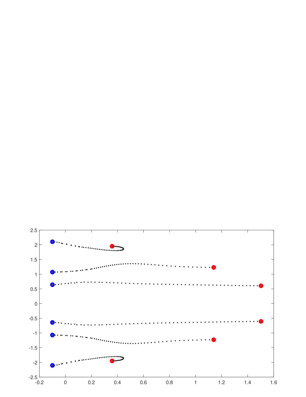
  Fig. 1.1: Paths of the eigenvalues of the matrix $A+\varepsilon E(\varepsilon)$ for $\varepsilon\in[0,\varepsilon_{\star}]$.

VI.1.2 Interior two-level algorithm

In the previous subsection, we worked with perturbed matrices that had some eigenvalues of positive real part, and the algorithm moved them to the left until it terminated with a matrix all of whose eigenvalues had real part at most $-\delta$. In an alternative approach, the given matrix $A$ is first perturbed to a non-optimal matrix $A+\varepsilon_{0}E_{0}$ with $\varepsilon_{0}>0$ and $E_{0}\in\mathcal{S}$ of unit Frobenius norm such that all its eigenvalues have real part smaller than $-\delta$. For example, this can be achieved by a simple shift if $I\in\mathcal{S}$. More importantly, the stable perturbed initial matrix $A+\varepsilon_{0}E_{0}$ may result from a non-optimal matrix stabilization algorithm. We then reduce the perturbation size while moving the rightmost eigenvalue towards the imaginary axis.

Using a two-level iteration starting from $A+\varepsilon_{0}E_{0}$, we aim to reduce the perturbation size to find $\varepsilon>0$ for which $A+\varepsilon E$ has some eigenvalue of real part at least $-\delta$ for every matrix $E$ of Frobenius norm 1. This differs from the problem of computing the distance to instability, where the aim was to find the smallest perturbation size $\varepsilon$ for which $A+\varepsilon E$ (with $A$ having only eigenvalues of negative real part) has eigenvalues of nonnegative real part for some matrix $E$ of Frobenius norm 1.

As in the algorithm for computing the distance to instability of Section IV.2, the target eigenvalue $\lambda(M)$ of a matrix $M$ is chosen as an eigenvalue of maximal real part. The function to be minimized is now $f(\lambda,\overline{\lambda})=+\,{\mbox{\rm Re}}\,\lambda$, whereas it was $f(\lambda,\overline{\lambda})=-\,{\mbox{\rm Re}}\,\lambda$ for computing the distance to instability of a Hurwitz matrix. Schematically, the interior two-level algorithm proceeds as follows.

• Inner iteration: Given $\varepsilon>0$, we aim to compute a matrix $E(\varepsilon)\in\mathcal{S}$ of unit Frobenius norm such that the rightmost eigenvalue of $A+\varepsilon E$ is minimized, i.e.

  $$E(\varepsilon)=\arg\min\limits_{E\in\mathcal{S},\|E\|_{F}=1}{\mbox{\rm Re}}\,\lambda(A+\varepsilon E).$$ (1.14)

  (Note that for computing the distance to instability, we maximized the same functional; see (2.1).)

• Outer iteration: We compute $\varepsilon_{\star}>0$ as the solution of the one-dimensional equation

  $$\phi(\varepsilon_{\star})=-\delta,$$ (1.15)

  where $\phi(\varepsilon)={\mbox{\rm Re}}\,\lambda(A+\varepsilon E(\varepsilon))$.

This yields the nearest perturbed matrix $A+\varepsilon_{\star}E(\varepsilon_{\star})$ with all eigenvalues of real part at most $-\delta$ and the perturbation matrix in the structure space $\mathcal{S}$.

In the inner iteration, the structured eigenvalue optimization problem (1.14) is of the class studied in Section V.2 and is solved with a rank-1 matrix differential equation as derived there.

In the outer iteration we compute the optimal perturbation size $\varepsilon_{\star}$ by the Newton–bisection algorithm of Section IV.1.5 for $f(\lambda,\overline{\lambda})={\mbox{\rm Re}}\,\lambda$, using the derivative formula of Theorem IV.IV.1.4 with $G(\varepsilon)=\Pi^{\mathcal{S}}(x(\varepsilon)y(\varepsilon)^{*})$; in particular, $G=xy^{*}$ in the complex unstructured case, and $G={\mbox{\rm Re}}(xy^{*})$ in the real unstructured case.

Numerical example

Consider the matrix

$$A=\left(\begin{array}[]{rrrrrrrrrr}0&1&1&1&-1&0&-1&0&0&0\\ 1&-1&0&1&1&0&1&0&0&0\\ -1&0&-1&-1&-1&1&1&1&0&0\\ 1&0&0&-1&1&-1&-1&1&0&0\\ 0&0&-1&1&0&1&1&-1&0&0\\ 0&-1&1&1&-1&0&0&1&1&0\\ -1&1&-1&1&1&0&-1&0&1&1\\ 0&0&1&-1&-1&1&1&1&-1&1\\ 0&0&0&0&0&0&0&-1&1&-1\\ 0&0&0&0&0&0&0&0&-1&1\end{array}\right)$$ (1.16)

The matrix $A$ has $6$ eigenvalues with positive real part. We set $\delta=0.1$.

Exterior method.

The stabilized matrix presents $7$ eigenvalues on the parallel axis to the imaginary axis and abscissa $-\delta=-0.1$; its distance from $A$ is $\varepsilon_{\star}\approx 2.56$. For comparison, the stabilized matrix computed by the algorithm of Orbandexivry, Nesterov & Van Dooren (?) has a much larger distance $9.02$ and all eigenvalues are located on the imaginary axis.

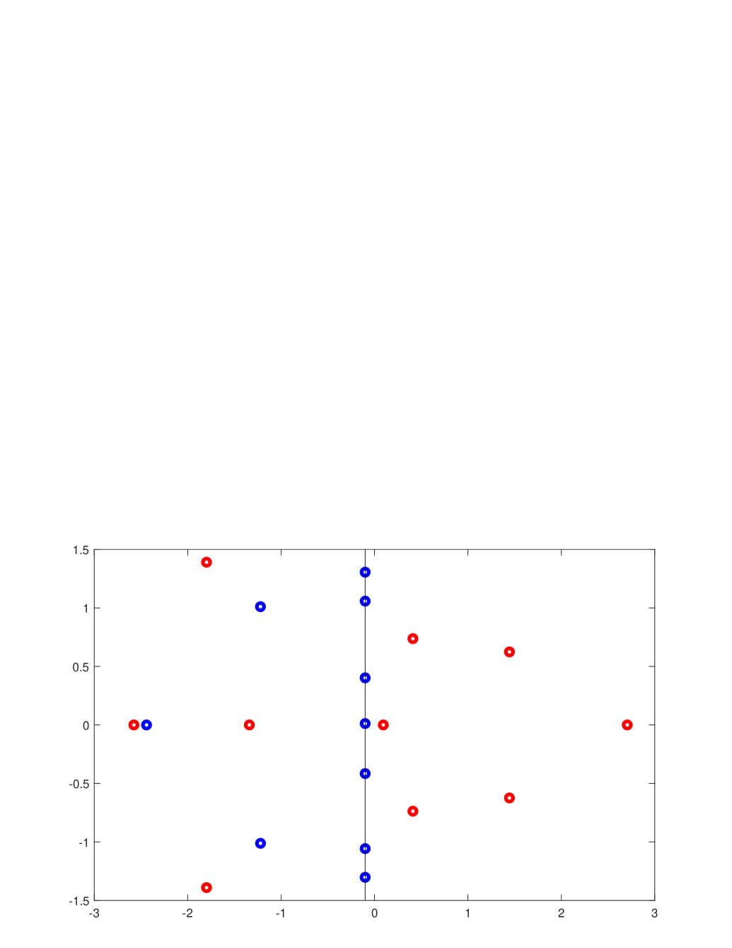
Fig. 1.2: Spectrum of the matrix (1.16) (gray circles) and of the stabilized matrix $A+\varepsilon_{\star}E(\varepsilon_{\star})$ (black circles) in the exterior method.

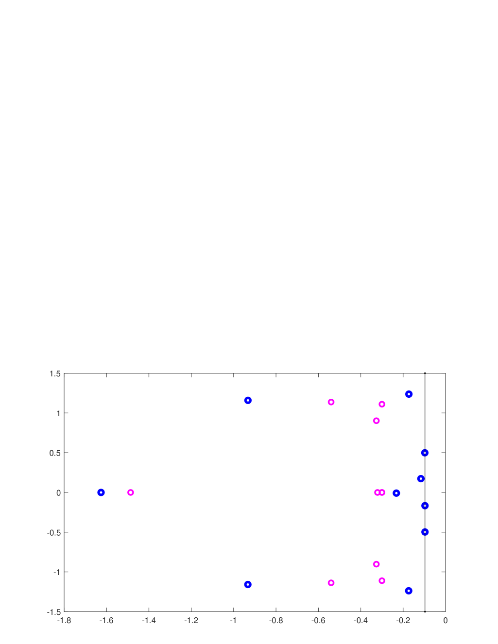
Fig. 1.3: Spectrum of the initial matrix stabilizing (1.16), computed by Overton’s algorithm (gray circles) and of the matrix $A+\varepsilon_{\star}E(\varepsilon_{\star})$ (black circles) computed by the interior method.

Interior method.

We start by computing a stable matrix, with spectrum on the left of the half-line ${\mbox{\rm Re}}z={}-\delta$, by using a method developed by Michael Overton, using a BFGS-type method on the penalized functional

$$\|X-A\|_{F}+\rho\,\alpha(X)$$

where $\alpha(X)$ denotes the spectral abscissa of $X$ and $\rho$ is a penalty parameter. We obtain in this way an initial matrix for our method, whose distance from $A$ is approximately $3.14$. After applying our interior method we obtain a stabilized matrix which has $3$ eigenvalues on the vertical axis with abscissa $-\delta=-0.1$; its distance from $A$ is $\varepsilon_{\star}\approx 2.94$, which is larger than the distance computed by the exterior method, but still a nearby matrix.

The method proposed by Gillis and Sharma (?) yields a stabilized matrix with approximate distance $1.92$ for $\delta=0$. The matrix has the double eigenvalue $0$ and further $4$ eigenvalues approximately aligned on the imaginary axis. We applied our interior method starting from the matrix computed by the algorithm by Gillis and Sharma (?). According to our experiments, this matrix turns out to be optimal also with respect to our method.

We refer to Guglielmi & Lubich (?) for numerical experiments of matrix stabilization for large sparse matrices, done with a numerical method that is closely related to the exterior method considered here, and for numerical comparisons with other methods.

VI.2 Hamiltonian matrix nearness problems

In this section we apply the two-level algorithmic approach of Chapter IV to matrix nearness problems for real Hamiltonian matrices, where ‘nearest’ again refers to the smallest distance in the Frobenius norm:

• Problem A.  Given a Hamiltonian matrix with no eigenvalues on the imaginary axis, find a nearest Hamiltonian matrix having some purely imaginary eigenvalue.

• Problem B.  Given a Hamiltonian matrix with some eigenvalues on the imaginary axis, find a nearest Hamiltonian matrix such that arbitrarily close to that matrix there exist Hamiltonian matrices with no eigenvalues on the imaginary axis.

Such and related Hamiltonian matrix nearness problems arise in the passivation of linear time-invariant control systems and in the stabilization of gyroscopic systems; see the references in the notes at the end of this chapter.

We deal here with structured matrix nearness problems with the structure space ${\mathcal{S}}$ given as the space $\text{Ham}(\mathbb{R}^{n,n})$ of real Hamiltonian matrices (with even dimension $n=2d$), consisting of those matrices $A\in\mathbb{R}^{n,n}$ for which

$$JA\,\hbox{ is real symmetric, where }\,J=\begin{pmatrix}0&I_{d}\\ -I_{d}&0\end{pmatrix}.$$

We note that the eigenvalues of a real Hamiltonian matrix lie symmetric to both the real axis and the imaginary axis: with any eigenvalue $\lambda$, also $\overline{\lambda},-\lambda,-\overline{\lambda}$ are eigenvalues. In fact, if $x$ is a left eigenvector of $A$ to the eigenvalue $\lambda$, then $Jx$ is a right eigenvector of $A$ to the eigenvalue $-\overline{\lambda}$, since $AJx=J^{-1}(JA)Jx=-JA^{\top}J^{\top}Jx=-J(x^{*}A)^{*}=-\overline{\lambda}Jx.$

VI.2.1 Problem A: Moving eigenvalues to the imaginary axis

For a real Hamiltonian matrix $M$, we let in the following the target eigenvalue $\lambda(M)$ be the eigenvalue of minimal real part in the first quadrant $\{\lambda\in\mathbb{C}\,:\,{\mbox{\rm Re}}\,\lambda\geq 0,\,{\mbox{\rm Im}}\,\lambda\geq 0\}$. (If this eigenvalue is not unique, we choose the one with minimal imaginary part.) We follow the two-level approach of Chapter IV:

• Inner iteration: Given $\varepsilon>0$, we aim to compute a matrix $E(\varepsilon)\in\mathcal{S}=\mathrm{Ham}(\mathbb{R}^{n,n})$ of unit Frobenius norm, such that ${\mbox{\rm Re}}\,\lambda(A+\varepsilon E)$ is minimized:

  $$E(\varepsilon)=\arg\min\limits_{E\in\mathrm{Ham}(\mathbb{R}^{n,n}),\|E\|_{F}=1}{\mbox{\rm Re}}\,\lambda(A+\varepsilon E).$$ (2.1)

• Outer iteration: We compute the smallest positive value $\varepsilon_{\star}$ with

  $$\phi(\varepsilon_{\star})=0,$$ (2.2)

  where $\phi(\varepsilon)={\mbox{\rm Re}}\,\lambda(A+\varepsilon E(\varepsilon))$.

We note that the inner iteration aims to find a leftmost point, in the first quadrant, of the structured $\varepsilon$-pseudospectrum $\Lambda_{\varepsilon}^{\mathcal{S}}(A)=\{\lambda\in\mathbb{C}\,:\,\text{$\lambda$ is an eigenvalue of $A+\varepsilon E$ for some}$ $E\in\mathcal{S}$ with $\|E\|_{F}=1\}$.

We recall from Section V.2.2 that the orthogonal projection $\Pi_{\mathcal{S}}$ from $\mathbb{C}^{n,n}$ onto ${\mathcal{S}}=\text{Ham}(\mathbb{R}^{n,n})$ is given by

$$\Pi^{\mathcal{S}}Z=J^{-1}\mathrm{Sym}({\mbox{\rm Re}}\,JZ),\qquad Z\in\mathbb{C}^{n,n}.$$ (2.3)

We already know from Section V.2.3 that if $\lambda(A+\varepsilon E(\varepsilon))$ is a simple eigenvalue, then the optimizer $E(\varepsilon)$ is a stationary point of the structure-constrained gradient flow given in (II.2.6), viz.,

$$\dot{E}=-G_{\varepsilon}^{\mathcal{S}}(E)+{\mbox{\rm Re}}\langle G_{\varepsilon}^{\mathcal{S}}(E),E\rangle E$$

$$\text{with the projected gradient }\ G_{\varepsilon}^{\mathcal{S}}(E)=\Pi^{\mathcal{S}}(xy^{*}),$$ (2.4)

where $x$ and $y$ are again left and right eigenvectors of $A+\varepsilon E$ with $\|x\|=\|y\|=1$ and $x^{*}y>0$. With the given definitions and the orthogonality of $J$, this becomes

$$J\dot{E}=-\mathrm{Sym}({\mbox{\rm Re}}\,Jxy^{*})+\langle\mathrm{Sym}({\mbox{\rm Re}}\,Jxy^{*}),JE\rangle JE.$$ (2.5)

In a stationary point, $E$ is a real multiple of $G_{\varepsilon}^{\mathcal{S}}(E)=J^{-1}\mathrm{Sym}({\mbox{\rm Re}}\,Jxy^{*})$, which is of rank at most 4. The precise rank is as follows.

• (Rank of optimizers).  For a real Hamiltonian matrix $A$ and $\varepsilon>0$, let $E\in\mathbb{R}^{n,n}$ with $\|E\|_{F}=1$ be a stationary point of the differential equation (2.5) such that the eigenvalue $\lambda=\lambda(A+\varepsilon E)$ is simple and $\lambda\notin\mathrm{i}\mathbb{R}$. Then,

  • $E$ has rank $4$ if $\lambda\notin\mathbb{R}$.

  • $E$ has rank $2$ if $\lambda\in\mathbb{R}$.

• If $x$ is a left eigenvector to the eigenvalue $\lambda$, then $Jx$ is a right eigenvector to $-\overline{\lambda}$. For a real Hamiltonian matrix, we have in addition that $J\overline{x}$ and $\overline{y}$ are eigenvectors to $-\lambda$ and $\overline{\lambda}$, respectively.

Under the assumption $\lambda\notin\mathbb{R}\cup\mathrm{i}\mathbb{R}$ we have four different eigenvalues lying symmetric to the real as well as the imaginary axis. The corresponding right eigenvectors $Jx,J\overline{x},y,\overline{y}$ are linearly independent, and so are their real and imaginary parts $Jx_{R},y_{R},Jx_{I},y_{I}$. Therefore, the matrix $JG_{\varepsilon}^{\mathcal{S}}(E))$, which is proportional to $JE$, equals

$$\mathrm{Sym}({\mbox{\rm Re}}\,Jxy^{*})=\tfrac{1}{4}(Jx_{R},y_{R},Jx_{I},y_{I})\begin{pmatrix}0&1&0&0\\ 1&0&0&0\\ 0&0&0&1\\ 0&0&1&0\end{pmatrix}(Jx_{R},y_{R},Jx_{I},y_{I})^{T},$$

which has rank 4. Hence, $G_{\varepsilon}^{\mathcal{S}}(E)=J^{-1}\mathrm{Sym}(J\,{\mbox{\rm Re}}\,xy^{*})$ has rank $4$, and so has its nonzero real multiple $E$.

If $\lambda$ is real and nonzero, then $Jx$ and $y$ are real, and they are linearly independent as eigenvectors to $-\lambda$ and $\lambda$. It follows that $G_{\varepsilon}^{\mathcal{S}}(E)$ and hence $E$ are of rank 2.   $\sqcap$$\sqcup$

VI.2.2 Inner iteration: Rank-4 constrained gradient flow

In view of Theorem VI.2.1, we restrict the gradient flow (2.4) to Hamiltonian rank-4 matrices, i.e., $JE$ will be constrained to lie in the manifold of symmetric rank-4 matrices and hence can be represented as

$$JE=USU^{\top},$$

where $U\in\mathbb{R}^{n\times 4}$ has orthonormal columns and $S\in\mathbb{R}^{4\times 4}$ is symmetric and invertible. Like in Section V.1.3, the orthogonal projection onto the tangent space at $JE$ is given as

$$P_{JE}(Z)=Z-(I-UU^{\top})Z(I-UU^{\top}),\qquad Z\in\mathbb{R}^{n\times n}.$$

We consider the rank-4 projected gradient flow

$$J\dot{E}=P_{JE}\Bigl{(}-\mathrm{Sym}({\mbox{\rm Re}}\,Jxy^{*})+\langle\mathrm{Sym}({\mbox{\rm Re}}\,Jxy^{*}),JE\rangle JE\Bigr{)},$$ (2.6)

where $x$ and $y$ are again left and right eigenvectors of $A+\varepsilon E$ with $\|x\|=\|y\|=1$ and $x^{*}y>0$ to the target eigenvalue $\lambda(A+\varepsilon E)$. Similarly to Sections II.3.3 and V.1.4, we have the following properties.

• (Monotonicity).  Let $E(t)$ of unit Frobenius norm be a solution to the differential equation (2.6). If the eigenvalue $\lambda(t)=\lambda(A+\varepsilon E(t))$ is simple, then

  $$\frac{d}{dt}\,{\mbox{\rm Re}}\,\lambda(t)\leq 0.$$ (2.7)

• We abbreviate $G=G_{\varepsilon}^{\mathcal{S}}(E)=J^{-1}\mathrm{Sym}({\mbox{\rm Re}}\,Jxy^{*})$ and obtain from (II.2.4) with $f(\lambda,\overline{\lambda})=\tfrac{1}{2}(\lambda+\overline{\lambda})={\mbox{\rm Re}}\,\lambda$ and $\kappa=1/(x^{*}y)>0$, using the orthogonality of $J$,

  $$\frac{1}{\varepsilon\kappa}\,\frac{d}{dt}\,{\mbox{\rm Re}}\,\lambda(t) =\langle G,\dot{E}\rangle=\langle JG,J\dot{E}\rangle$$

  $$=\langle JG,P_{JE}\bigl{(}-JG-\langle JG,JE\rangle E\bigr{)}\rangle$$

  $$=\Bigl{(}-\|P_{JE}(JG)\|_{F}^{2}+\bigl{(}{\mbox{\rm Re}}\,\langle P_{JE}(JG),JE\rangle\bigr{)}^{2}\Bigr{)}\leq 0,$$ (2.8)

  where we used $P_{JE}(JE)=JE$ in the last equality, and $\|JE\|_{F}=1$ and the Cauchy–Schwarz inequality in the final inequality.   $\sqcap$$\sqcup$

  • (Stationary points).  Let $E$ be a real Hamiltonian rank-4 matrix of unit Frobenius norm and suppose that $P_{JE}(JG_{\varepsilon}^{\mathcal{S}}(E))\neq 0$. If $E$ is a stationary point of the projected differential equation (2.6), then $E$ is already a stationary point of the differential equation (2.4).

    • The proof is similar to the proof of Theorem II.V.1.4. We show that $E$ is a real multiple of $G_{\varepsilon}^{\mathcal{S}}(E)$. By (II.2.8), $E$ is then a stationary point of the differential equation (II.2.6), which is the same as (2.4).

      For a stationary point $E$ of (2.6), we must have equality in the estimate of the previous proof, which shows that $P_{JE}(JG)$ (with $G=G_{\varepsilon}^{\mathcal{S}}(E)$) is a nonzero real multiple of $E$. Hence, in view of $P_{JE}(JE)=JE$, we can write $G$ as

      $$G=\mu E+W,\quad\text{ where $\mu\neq 0$ and $P_{JE}(JW)=0$.}$$

      With $JE=USU^{\top}$ as above, we then have

      $$JW=JW-P_{JE}(JW)=(I-UU^{\top})JW(I-UU^{\top}).$$

      Since $G$ is of rank at most $4$ and real Hamiltonian, it can be written in the form $JG=XRX^{\top}$, where $X\in\mathbb{R}^{n,4}$ has orthonormal columns and $R\in\mathbb{R}^{4,4}$. So we have

      $$XRX^{\top}=\mu USU^{\top}+(I-UU^{\top})JW(I-UU^{\top}).$$

      Multiplying from the right with $U$ yields $X(RX^{\top}U)=\mu US$, which shows that $X$ has the same range as $U$. Hence, $JG$ has the same range as $JE$, which implies that $P_{JE}(JG)=JG$. Since we already know that $P_{JE}(JG)$ is a nonzero real multiple of $P_{JE}(JE)=JE$, it follows that $G$ is the same real multiple of $E$. Hence $E$ is a stationary point of (2.4).   $\sqcap$$\sqcup$

      We further remark that for real simple eigenvalues $\lambda$ we have an analogous rank-2 dynamics.

A robust integrator.

The following time-stepping method is an adaptation to (2.6) of the low-rank integrator of Ceruti & Lubich (?), similar to the integrator in Section V.1.5. It first updates the basis matrix $U$ with orthonormal columns and then computes an update of the symmetric $4\times 4$ matrix $S$ by a Galerkin approximation to the differential equation (2.6) in the updated basis. This integrator is robust to the presence of small singular values, which appear in the case of a target eigenvalue near the real axis, where the rank degenerates from 4 to 2.

One time step of integration from time $t_{k}$ to $t_{k+1}=t_{k}+h$ starting from a factored rank-$4$ matrix $JE_{k}=U_{k}S_{k}U_{k}^{\top}$ of unit Frobenius norm computes an updated rank-$r$ factorization $JE_{k+1}=U_{k+1}S_{k+1}U_{k+1}^{\top}$ of unit Frobenius norm as follows.

1. Update the basis matrix $U_{k}\rightarrow U_{k+1}$:
   Integrate from $t=t_{k}$ to $t_{k+1}=t_{k}+h$ the $n\times r$ matrix differential equation

   $$\dot{K}(t)=-JG_{\varepsilon}^{\mathcal{S}}(K(t)U_{k}^{\top})U_{k},\qquad K(t_{k})=U_{k}S_{k}.$$

   Perform a QR factorization $K(t_{k+1})=U_{k+1}{R}_{k+1}$ and compute the $r\times r$ matrix $M=U_{k+1}^{\top}U_{k}$.
   

2. Update the symmetric matrix ${S}_{k}\rightarrow{S}_{k+1}$ :
   Integrate from $t=t_{k}$ to $t_{k+1}$ the $r\times r$ matrix differential equation

   $$\dot{S}(t)=-U_{k+1}^{\top}JG_{\varepsilon}^{\mathcal{S}}(U_{k+1}S(t)U_{k+1}^{\top})U_{k+1},\qquad S(t_{k})=\frac{M{S}_{k}M^{\top}}{\|M{S}_{k}M^{\top}\|_{F}},$$

   and set ${S}_{k+1}=S(t_{k+1})/\|S(t_{k+1})\|_{F}$.

The differential equations in the substeps are solved approximately by a step of some standard numerical integrator, e.g. the explicit Euler method or a low-order explicit Runge–Kutta method such as the second-order Heun method. The stepsize selection is done as in Section V.1.5, using an Armijo-type line search.

VI.2.3 Eigenvalues close to coalescence on the imaginary axis

This theoretical section serves as a preparation for the algorithm of the outer iteration that will be presented in the next section. Let $E(\varepsilon)$ of unit Frobenius norm be a local minimizer of the optimization problem (2.1). We let $\lambda(\varepsilon)$ be the eigenvalue of smallest positive real part (and nonnegative imaginary part) of the Hamiltonian matrix

$$M(\varepsilon):=A+\varepsilon E(\varepsilon)$$

and $x(\varepsilon)$ and $y(\varepsilon)$ are corresponding left and right eigenvectors normalized by $\|x(\varepsilon)\|=\|y(\varepsilon)\|=1$ and $x(\varepsilon)^{*}y(\varepsilon)>0$. We let $\varepsilon_{\star}$ be the smallest value of $\varepsilon$ such that

$$\phi(\varepsilon)={\mbox{\rm Re}}\,\lambda(\varepsilon)$$

becomes zero:

$$\phi(\varepsilon)>0\quad\ \text{for }0<\varepsilon<\varepsilon_{\star}\quad\ \text{ and }\quad\phi(\varepsilon)=0\quad\text{for $\varepsilon\geq\varepsilon_{\star}$ near $\varepsilon_{\star}$.}$$

Under Assumption IV.IV.1.4, the function $\phi$ is continuously differentiable in a left neighbourhood of $\varepsilon_{\star}$ and its derivative is given by Theorem IV.IV.1.4. In the following we show that under further assumptions, the function $\phi$ has a square-root behavior $\phi(\varepsilon)\sim\sqrt{\varepsilon_{\star}-\varepsilon}$ as $\varepsilon\nearrow\varepsilon_{\star}$.

• We assume that the limit $M(\varepsilon_{\star}):=\lim_{\varepsilon\nearrow\varepsilon_{\star}}M(\varepsilon)$ of the Hamiltonian matrices exists and that the purely imaginary eigenvalue $\lambda(\varepsilon_{\star})=\lim_{\varepsilon\nearrow\varepsilon_{\star}}\lambda(\varepsilon)$ of $M(\varepsilon_{\star})$ has algebraic multiplicity two and is defective (that is, the zero singular value of $M(\varepsilon_{\star})-\lambda(\varepsilon_{\star})I$ is simple).

  By definition of $\varepsilon_{\star}$, the eigenvalue $\lambda(\varepsilon_{\star})$ is on the imaginary axis and has even multiplicity because of the symmetry of the eigenvalues with respect to the imaginary axis. Here we assume multiplicity two. The defectivity appears to be generic (we have no proof for this but observed defectivity in all our numerical experiments).

  Under Assumption VI.2.3, the eigenvalue $\lambda(\varepsilon_{\star})$ of $M(\varepsilon_{\star})$ is non-derogatory, that is, only a single Jordan block corresponds to this eigenvalue, and hence its left and right eigenspaces are of dimension 1. Since $\lambda(\varepsilon_{\star})$ is a defective eigenvalue, left and right eigenvectors at $\varepsilon_{\star}$ are orthogonal to each other: $x(\varepsilon_{\star})^{*}y(\varepsilon_{\star})=0$.

We need the following result.

• (Eigenvectors at coalescence).  Let $M(\varepsilon)$, $\varepsilon\in[\varepsilon_{0},\varepsilon_{\star}]$, be a continuous path of real Hamiltonian matrices, and $\lambda(\varepsilon)$ be a path of eigenvalues of $M(\varepsilon)$ that are simple and not purely imaginary for $\varepsilon<\varepsilon_{\star}$ and satisfy Assumption VI.2.3 at $\varepsilon_{\star}$. Under a nondegeneracy condition on eigenvectors of $M(\varepsilon)$ stated in (2.20) below, there exist left and right eigenvectors $x(\varepsilon)$ and $y(\varepsilon)$ to the eigenvalue $\lambda(\varepsilon)$, normalized to unit norm and with $x(\varepsilon)^{*}y(\varepsilon)>0$ for $\varepsilon<\varepsilon_{\star}$, which depend continuously on $\varepsilon$ in the closed interval $[\varepsilon_{0},\varepsilon_{\star}]$. In particular, the eigenvectors converge for $\varepsilon\nearrow\varepsilon_{\star}$. In the limit we have

  $$y(\varepsilon_{\star})=\pm Jx(\varepsilon_{\star}),$$

  where the sign depends on $x(\varepsilon)$ for $\varepsilon$ near $\varepsilon_{\star}$.

  The important fact here is that $y(\varepsilon_{\star})$ is not just a complex multiple of $Jx(\varepsilon_{\star})$, as would easily be obtained from the symmetry of eigenvalues with respect to the imaginary axis, but that it is a real multiple.

  • By a result of Paige & Van Loan (?), Theorem 5.1, the Hamiltonian matrix $M(\varepsilon)$ with no imaginary eigenvalues (for $\varepsilon<\varepsilon_{\star}$) admits a real Schur-Hamiltonian decomposition, that is, there exists an orthogonal symplectic real matrix $S(\varepsilon)$ (i.e., $S(\varepsilon)^{\top}S(\varepsilon)=I$ and $S(\varepsilon)^{\top}JS(\varepsilon)=J$) for $\varepsilon>\varepsilon_{\star}$) that transforms $M(\varepsilon)$ to a block triangular Hamiltonian matrix

    $$M_{0}(\varepsilon)=S(\varepsilon)^{-1}M(\varepsilon)S(\varepsilon)=\begin{pmatrix}F(\varepsilon)&H(\varepsilon)\\ 0&-F(\varepsilon)^{\top}\end{pmatrix},$$ (2.9)

    where $H(\varepsilon)$ is symmetric and $F(\varepsilon)$ is upper quasi-triangular.

    For the eigenvalue $\lambda(\varepsilon)$, the left and right eigenvectors of $M_{0}(\varepsilon)$ are related to those of $M(\varepsilon)$ by

    $$x_{0}(\varepsilon)=S(\varepsilon)^{\top}x(\varepsilon),\qquad y_{0}(\varepsilon)=S(\varepsilon)^{-1}y(\varepsilon).$$ (2.10)

    We assume that $x(\varepsilon)$ and $y(\varepsilon)$ are normalized to norm 1 and such that $x(\varepsilon)^{*}y(\varepsilon)>0$ for $\varepsilon>\varepsilon_{\star}$, and hence we have also

    $$\text{$x_{0}(\varepsilon)$ and $y_{0}(\varepsilon)$ are of norm 1 and\ }\ x_{0}(\varepsilon)^{*}y_{0}(\varepsilon)>0.$$ (2.11)

    We observe that the lower half of the right eigenvector $y_{0}(\varepsilon)$ to the block triangular matrix $M_{0}(\varepsilon)$ consists only of zeros and we split the eigenvectors into the upper and the lower $n/2$-dimensional subvectors as

    $$y_{0}(\varepsilon)=\left(\begin{array}[]{r}-p(\varepsilon)\\ 0\end{array}\right),\qquad x_{0}(\varepsilon)=\left(\begin{array}[]{r}-s(\varepsilon)\\ r(\varepsilon)\end{array}\right).$$ (2.12)

    By the Hamiltonian symmetry, left and right eigenvectors associated with the eigenvalue $-\overline{\lambda(\varepsilon)}$, with positive inner product, are $\widetilde{x}_{0}(\varepsilon)=Jy_{0}(\varepsilon)$ and $\widetilde{y}_{0}(\varepsilon)=Jx_{0}(\varepsilon)$, and so we have

    $$\widetilde{y}_{0}(\varepsilon)=\left(\begin{array}[]{r}r(\varepsilon)\\ s(\varepsilon)\end{array}\right),\qquad\widetilde{x}_{0}(\varepsilon)=\left(\begin{array}[]{r}0\\ p(\varepsilon)\end{array}\right).$$ (2.13)

    By compactness, there exists a sequence $(\varepsilon_{n})$ with $\varepsilon_{n}\nearrow\varepsilon_{\star}$ as $n\to\infty$ such that $x_{0}(\varepsilon_{n})$, $y_{0}(\varepsilon_{n})$ and $S(\varepsilon_{n})$ converge to vectors $x_{0,\star}$, $y_{0,\star}$ of norm 1 and an orthogonal symplectic real matrix $S_{\star}$. By the continuity of $M(\cdot)$ and $\lambda(\cdot)$ at $\varepsilon_{\star}$, the limit vectors $x_{0,\star}$, $y_{0,\star}$ are then left and right eigenvectors corresponding to the purely imaginary eigenvalue $\lambda(\varepsilon_{\star})$ of $M(\varepsilon_{\star})$.

    By Assumption VI.2.3, the left and right eigenspaces to $\lambda(\varepsilon_{\star})$ are one-dimensional, and so we have that for some complex $\xi,\eta$ of unit modulus,

    $$\lim\limits_{n\to\infty}\widetilde{y}_{0}(\varepsilon_{n})=-\eta\lim\limits_{n\to\infty}y_{0}(\varepsilon_{n}),\qquad\lim\limits_{n\to\infty}\widetilde{x}_{0}(\varepsilon_{n})=\xi\lim\limits_{n\to\infty}x_{0}(\varepsilon_{n}).$$ (2.14)

    We thus obtain

    $$\lim_{n\to\infty}s(\varepsilon_{n})=0$$ (2.15)

    and

    $$\lim\limits_{n\to\infty}r(\varepsilon_{n})=\eta\lim\limits_{n\to\infty}p(\varepsilon_{n}),\qquad\lim\limits_{n\to\infty}p(\varepsilon_{n})=\xi\lim\limits_{n\to\infty}r(\varepsilon_{n}),$$ (2.16)

    so that

    $$\xi=\bar{\eta}.$$ (2.17)

    By (2.11),

    $$s(\varepsilon)^{*}p(\varepsilon)\ \text{ is real and positive for }\varepsilon>\varepsilon_{\star},$$ (2.18)

    and in particular, $s(\varepsilon)\neq 0$ for $\varepsilon>\varepsilon_{\star}$ (but recall (2.15)).

    Moreover, from the fact that $x_{0}(\varepsilon)$ is a left eigenvalue of $M_{0}(\varepsilon)$, we infer that (omitting the argument $\varepsilon$ in the next few lines) $s^{*}F=\lambda s^{*}$ and $-s^{*}H-r^{*}F^{\top}=\lambda r^{*}$. Multiplying the second equation with $s$ from the right and using the first equation then yields $-s^{*}Hs=(\lambda+\overline{\lambda})\,r^{*}s$, which shows that

    $$s(\varepsilon)^{*}r(\varepsilon)\ \text{ is real for }\varepsilon>\varepsilon_{\star}.$$ (2.19)

    Under the nondegeneracy condition

    $$\liminf_{\varepsilon\nearrow\varepsilon_{\star}}\,\left|\left(\frac{s(\varepsilon)}{\|s(\varepsilon)\|}\right)^{*}\frac{r(\varepsilon)}{\|r(\varepsilon)\|}\right|>0,$$ (2.20)

    which states that the normalizations of the vectors $s$ and $r$ are not asymptotically orthogonal, we conclude that there is a subsequence $(\varepsilon_{n}^{\prime})$ of $(\varepsilon_{n})$ such that the normalized sequence $\bigl{(}s(\varepsilon_{n}^{\prime})/\|s(\varepsilon_{n}^{\prime})\|\bigr{)}$ is convergent and (on noting that $\|r(\varepsilon_{n})\|\to 1$ because of (2.12) and (2.15))

    $$\lim_{n\to\infty}\frac{s(\varepsilon_{n}^{\prime})^{*}r(\varepsilon_{n}^{\prime})}{\|s(\varepsilon_{n}^{\prime})\|}\neq 0.$$ (2.21)

    As (2.16) implies that this nonzero limit equals

    $$\lim_{n\to\infty}\frac{s(\varepsilon_{n}^{\prime})^{*}r(\varepsilon_{n}^{\prime})}{\|s(\varepsilon_{n}^{\prime})\|}=\eta\lim_{n\to\infty}\frac{s(\varepsilon_{n}^{\prime})^{*}p(\varepsilon_{n}^{\prime})}{\|s(\varepsilon_{n}^{\prime})\|}$$

    and the two limits in this formula are real by (2.18) and (2.19), it follows that $\eta$ is real and hence $\eta$ equals $1$ or $-1$. In view of $\eqref{sp-pos}$ and (2.20), we actually have

    $$\eta=\lim_{\varepsilon\nearrow\varepsilon_{\star}}\ \mathrm{sign}(s(\varepsilon)^{*}r(\varepsilon))=\pm 1,$$ (2.22)

    which depends only on the left eigenvector $x_{0}(\varepsilon)$. As a consequence, we obtain from (2.14) that

    $$y_{0,\star}=-\eta Jx_{0,\star}=\mp Jx_{0,\star}.$$ (2.23)

    By (2.10) we have

    $$x(\varepsilon)=\left(S(\varepsilon)^{\top}\right)^{-1}x_{0}(\varepsilon)=-JS(\varepsilon)Jx_{0}(\varepsilon),\qquad y(\varepsilon)=S(\varepsilon)y_{0}(\varepsilon)=\pm S(\varepsilon)Jx_{0}(\varepsilon)$$ (2.24)

    and therefore the limits $x_{\star}=\lim_{n\to\infty}x(\varepsilon_{n})$ and $y_{\star}=\lim_{n\to\infty}y(\varepsilon_{n})$ exist and satisfy

    $$y_{\star}=\pm Jx_{\star}.$$ (2.25)

    We now use once again that by Assumption VI.2.3, the left and right eigenspaces to $\lambda(\varepsilon_{\star})$ are one-dimensional. Hence $x_{\star}$ is a complex multiple of the unique left eigenvector $x(\varepsilon_{\star})$ of norm 1 for which the first nonzero entry is positive. If we choose the eigenvectors $x(\varepsilon)$ such that their corresponding entry is also nonnegative, then we find that every convergent subsequence $(x(\varepsilon_{n}))$ converges to the same limit $x(\varepsilon_{\star})$ as $n\to\infty$, and hence $x(\varepsilon)$ converges to $x(\varepsilon_{\star})$ as $\varepsilon\nearrow\varepsilon_{\star}$. To the left eigenvector $x(\varepsilon)$, there corresponds a unique right eigenvector $y(\varepsilon)$ of norm 1 that satisfies $x(\varepsilon)^{*}y(\varepsilon)>0$ for $\varepsilon>\varepsilon_{\star}$. By (2.25), the limit of every convergent subsequence $(y(\varepsilon_{n}))$ converges to $\pm J\lim_{n\to\infty}x(\varepsilon_{n})=\pm Jx(\varepsilon_{\star})$, and hence the limit $y(\varepsilon_{\star}):=\lim_{\varepsilon\nearrow\varepsilon_{\star}}y(\varepsilon)$ exists, is a right eigenvector of $M(\varepsilon_{\star})$ to the eigenvalue $\lambda(\varepsilon_{\star})$, and it equals

    $$y(\varepsilon_{\star})=\lim_{\varepsilon\nearrow\varepsilon_{\star}}y(\varepsilon)=\pm J\lim_{\varepsilon\nearrow\varepsilon_{\star}}x(\varepsilon)=\pm Jx(\varepsilon_{\star}),$$

    which completes the proof.   $\sqcap$$\sqcup$

    • If additionally $M(\varepsilon)$, $\varepsilon\in[\varepsilon_{0},\varepsilon_{\star}]$, is continuously differentiable and ${\mbox{\rm Re}}\,x(\varepsilon_{\star})^{*}M^{\prime}(\varepsilon_{\star})y(\varepsilon_{\star})\neq 0$, then Theorem VI.2.3 implies that the eigenvalue $\lambda(\varepsilon)$ approaches the imaginary axis in normal direction (i.e. horizontally in the complex plane). This is because then we have, with $\kappa(\varepsilon)=1/(x(\varepsilon)^{*}y(\varepsilon))>0$,

      $${\mbox{\rm Im}}\,\frac{\lambda^{\prime}(\varepsilon)}{\kappa(\varepsilon)} ={\mbox{\rm Im}}\,x(\varepsilon)^{*}M^{\prime}(\varepsilon)y(\varepsilon)\to{\mbox{\rm Im}}\,x(\varepsilon_{\star})^{*}M^{\prime}(\varepsilon_{\star})y(\varepsilon_{\star})$$

      $$={\mbox{\rm Im}}\,(Jx(\varepsilon_{\star}))^{*}JM^{\prime}(\varepsilon_{\star})y(\varepsilon_{\star})=\pm\,{\mbox{\rm Im}}\,y(\varepsilon_{\star})^{*}JM^{\prime}(\varepsilon_{\star})y(\varepsilon_{\star})=0$$

      by the symmetry of $JM^{\prime}(\varepsilon_{\star})$. By assumption,

      $${\mbox{\rm Re}}\,\frac{\lambda^{\prime}(\varepsilon)}{\kappa(\varepsilon)}={\mbox{\rm Re}}\,x(\varepsilon)^{*}M^{\prime}(\varepsilon)y(\varepsilon)\to{\mbox{\rm Re}}\,x(\varepsilon_{\star})^{*}M^{\prime}(\varepsilon_{\star})y(\varepsilon_{\star})\neq 0.$$

      Hence, ${\mbox{\rm Im}}\,\lambda^{\prime}(\varepsilon)\,/\,{\mbox{\rm Re}}\,\lambda^{\prime}(\varepsilon)\to 0$ as $\varepsilon\nearrow\varepsilon_{\star}$. This can, however, not be concluded when $M^{\prime}(\varepsilon)$ has no limit at $\varepsilon_{\star}$ and $\|M^{\prime}(\varepsilon)\|\to\infty$ as $\varepsilon\nearrow\varepsilon_{\star}$.

    We are now in a position to characterize the asymptotic behaviour of the function $\phi(\varepsilon)={\mbox{\rm Re}}\,\lambda(\varepsilon)$ as $\varepsilon\nearrow\varepsilon_{\star}$, in the situation described at the beginning of this section.

    • (Square root asymptotics).  Under Assumptions IV.IV.1.4 and VI.2.3 and the nondegeneracy condition (2.20), and under the further condition that the eigenvalue $\lambda(\varepsilon)$ of the Hamiltonian matrix $M(\varepsilon)=A+\varepsilon E(\varepsilon)$ does not approach the imaginary axis tangentially as $\varepsilon\nearrow\varepsilon_{\star}$, we have

      $${\mbox{\rm Re}}\,\lambda(\varepsilon)=\gamma\,\sqrt{\varepsilon_{\star}-\varepsilon}\;(1+o(1))\quad\text{ as }\ \varepsilon\nearrow\varepsilon_{\star}$$

      for some positive constant $\gamma$.

    • We split the proof into four parts (a)-(d).
      (a) For $\varepsilon<\varepsilon_{\star}$, let $x(\varepsilon)$ and $y(\varepsilon)$ be left and right eigenvectors of $M(\varepsilon)=A+\varepsilon E(\varepsilon)$ to the simple eigenvalue $\lambda(\varepsilon)$, of unit norm and with $x(\varepsilon)^{*}y(\varepsilon)>0$ for $\varepsilon<\varepsilon_{\star}$ and normalized such that their limits for $\varepsilon\nearrow\varepsilon_{\star}$ exist according to Theorem VI.2.3. We consider the nonnegative function

      $$\vartheta(\varepsilon):=\frac{1}{\kappa(\varepsilon)}=x(\varepsilon)^{*}y(\varepsilon)>0\ \text{ for }\ \varepsilon\in(\varepsilon_{0},\varepsilon_{\star}),\qquad\vartheta(\varepsilon_{\star})=0.$$

      To compute the derivative of $\vartheta$, we use Theorem IX.IX.2 for the left and right eigenvectors of norm 1 and with positive inner product,

      $$x^{\prime}(\varepsilon)^{*} =-x(\varepsilon)^{*}M^{\prime}(\varepsilon)Z(\varepsilon)+{\mbox{\rm Re}}\bigl{(}x(\varepsilon)^{*}M^{\prime}(\varepsilon)Z(\varepsilon)x(\varepsilon)\bigr{)}x(\varepsilon)^{*}$$

      $$y^{\prime}(\varepsilon) =-Z(\varepsilon)M^{\prime}(\varepsilon)y(\varepsilon)+{\mbox{\rm Re}}\bigl{(}y(\varepsilon)^{*}Z(\varepsilon)M^{\prime}(\varepsilon)y(\varepsilon)\bigr{)}y(\varepsilon),$$

      where $Z(\varepsilon)$ is the group inverse of $N(\varepsilon):=M(\varepsilon)-\lambda(\varepsilon)I$. Since Theorem IX.IX.2 shows that $x(\varepsilon)^{*}Z(\varepsilon)=0$ and $Z(\varepsilon)y(\varepsilon)=0$, these formulas imply

      $$\vartheta^{\prime}(\varepsilon)={\mbox{\rm Re}}\Bigl{(}x(\varepsilon)^{*}M^{\prime}(\varepsilon)Z(\varepsilon)x(\varepsilon)+y(\varepsilon)^{*}Z(\varepsilon)M^{\prime}(\varepsilon)y(\varepsilon)\Bigr{)}\vartheta(\varepsilon).$$ (2.26)

      By Theorem IX.IX.2, the group inverse is related to the pseudoinverse $N(\varepsilon)^{\dagger}$ by the formulas

      $$Z(\varepsilon) = \frac{1}{\vartheta(\varepsilon)^{2}}\widehat{Z}(\varepsilon)$$

      $$\widehat{Z}(\varepsilon) = \bigl{(}\vartheta(\varepsilon)I-y(\varepsilon)x(\varepsilon)^{*}\bigr{)}N(\varepsilon)^{\dagger}\bigl{(}\vartheta(\varepsilon)I-y(\varepsilon)x(\varepsilon)^{*}\bigr{)}.$$ (2.27)

      By Assumption VI.2.3, the second smallest singular value $\sigma_{n-1}(\varepsilon)$ of $N(\varepsilon)$ does not converge to zero. Therefore, $N(\varepsilon)^{\dagger}$ has a finite limit as $\varepsilon\nearrow\varepsilon_{\star}$. We thus have

      $$\widehat{Z}(\varepsilon) = y(\varepsilon)x(\varepsilon)^{*}N(\varepsilon)^{\dagger}y(\varepsilon)x(\varepsilon)^{*}+O(\vartheta(\varepsilon))$$

      $$= \nu(\varepsilon)y(\varepsilon)x(\varepsilon)^{*}+O(\vartheta(\varepsilon))$$

      with the factor

      $$\nu(\varepsilon):=x(\varepsilon)^{*}N(\varepsilon)^{\dagger}y(\varepsilon),$$

      Furthermore, we set

      $$\mu(\varepsilon):=x(\varepsilon)^{*}M^{\prime}(\varepsilon)y(\varepsilon).$$

      We insert the expression for the group inverse $Z(\varepsilon)$ into (2.26) and note the identities $N^{\dagger}(\varepsilon)x(\varepsilon)=0$ and $y(\varepsilon)^{*}N^{\dagger}(\varepsilon)=0$, which follow from $x(\varepsilon)^{*}N(\varepsilon)=0$ and $N(\varepsilon)y(\varepsilon)=0$, respectively. We then obtain

      $$\vartheta^{\prime}(\varepsilon)\vartheta(\varepsilon) ={\mbox{\rm Re}}\Bigl{(}x(\varepsilon)^{*}M^{\prime}(\varepsilon)\widehat{Z}(\varepsilon)x(\varepsilon)+y(\varepsilon)^{*}\widehat{Z}(\varepsilon)M^{\prime}(\varepsilon)y(\varepsilon)\Bigr{)}$$

      $$={\mbox{\rm Re}}\Bigl{(}2\nu(\varepsilon)\mu(\varepsilon)+O(\vartheta(\varepsilon)\mu(\varepsilon))\Bigr{)}.$$ (2.29)

      (b) We now study the limit behaviour of $\nu(\varepsilon)$ as $\varepsilon\nearrow\varepsilon_{\star}$. By Theorem VI.2.3, the limits of the left and right eigenvectors for $\varepsilon\nearrow\varepsilon_{\star}$ exist and satisfy $y(\varepsilon_{\star})=\pm Jx(\varepsilon_{\star})$ and further $x(\varepsilon_{\star})^{*}y(\varepsilon_{\star})=0$. Since $JN(\varepsilon_{\star})$ is a hermitian matrix, we therefore obtain

      $$\nu(\varepsilon_{\star}) =x(\varepsilon_{\star})^{*}N(\varepsilon_{\star})^{\dagger}y(\varepsilon_{\star})=x(\varepsilon_{\star})^{*}(JN(\varepsilon_{\star}))^{\dagger}Jy(\varepsilon_{\star})$$

      $$=\mp\,x(\varepsilon_{\star})^{*}(JN(\varepsilon_{\star}))^{\dagger}x(\varepsilon_{\star})\in\mathbb{R}.$$

      We next show that $\nu(\varepsilon_{\star})\neq 0$. Since $x(\varepsilon_{\star})\,\bot\,y(\varepsilon_{\star})$ and since $x(\varepsilon_{\star})$ spans the nullspace of $N(\varepsilon_{\star})^{*}$ (by the defectivity condition in Assumption VI.2.3), we obtain

      $$y(\varepsilon_{\star})\in{\rm Ker}(N(\varepsilon_{\star})^{*})^{\perp}={\rm Range}\left(N(\varepsilon_{\star})\right).$$

      Hence there exists $z_{1}$ such that $y(\varepsilon_{\star})=N(\varepsilon_{\star})z_{1}$. Assume, in a proof by contradiction, $N(\varepsilon_{\star})^{\dagger}y(\varepsilon_{\star})\,\bot\,x(\varepsilon_{\star})$, which means

      $$N(\varepsilon_{\star})^{\dagger}y(\varepsilon_{\star})\in{\rm Range}\left(N(\varepsilon_{\star})\right).$$

      Hence there exists $z_{2}$ such that $N(\varepsilon_{\star})^{\dagger}y(\varepsilon_{\star})=N(\varepsilon_{\star})z_{2}$.

      Multiplying this equation with $N(\varepsilon_{\star})^{2}$ we obtain (omitting the argument $\varepsilon_{\star}$ in the following)

      $$N^{3}z_{2}=N^{2}N^{\dagger}y=N\,NN^{\dagger}Nz_{1}=NNz_{1}=Ny=0.$$

      The null-space of $N^{3}$ is two-dimensional by Assumption VI.2.3 and contains the two nonzero vectors $y$ and $N^{\dagger}y$, since $Ny=0$ and $N^{2}N^{\dagger}y=0$. Note that $N^{\dagger}y\neq 0$ because otherwise $y$ would be in the nullspace of $N^{\dagger}$, which is the nullspace of $N^{*}$, which contradicts the above observation that $y\neq 0$ is in the orthogonal complement of the nullspace of $N^{*}$. Moreover, $y$ and $N^{\dagger}y$ are linearly independent, since otherwise the relation $y=cN^{\dagger}y$ would yield, on multiplication with $N$, that

      $$0=Ny=cNN^{\dagger}y=cNN^{\dagger}Nz_{1}=cNz_{1}=cy,$$

      which contradicts $y\neq 0$. Therefore, the null-space of $N^{3}$ is spanned by $y$ and $N^{\dagger}y$, and since we have shown that it contains $z_{2}$, we obtain

      $$z_{2}=c_{1}y+c_{2}N^{\dagger}y.$$

      Multiplying this equation with $N$ then gives

      $$N^{\dagger}y=Nz_{2}=c_{2}NN^{\dagger}Nz_{1}=c_{2}Nz_{1}=c_{2}y,$$

      which contradicts the linear independence of $y$ and $N^{\dagger}y$. We have thus led the assumption $N(\varepsilon_{\star})^{\dagger}y(\varepsilon_{\star})\ \bot\ x(\varepsilon_{\star})$ to a contradiction. Therefore, $\nu(\varepsilon_{\star})\neq 0$. So we have shown that

      $$\nu_{\star}:=\lim_{\varepsilon\nearrow\varepsilon_{\star}}\nu(\varepsilon)\quad\text{exists and is real and nonzero.}$$ (2.30)

      (c) We next study the limit behaviour of $\mu(\varepsilon)$ as $\varepsilon\nearrow\varepsilon_{\star}$. By Theorem IX.IX.1 we have

      $$\mu(\varepsilon)=\lambda^{\prime}(\varepsilon)\vartheta(\varepsilon).$$

      By Theorem IV.IV.1.4 with the objective function $\phi(\varepsilon)={\mbox{\rm Re}}\,\lambda(\varepsilon)$ and the gradient $Z(\varepsilon)=\mathrm{Sym}({\mbox{\rm Re}}\,Jx(\varepsilon)y(\varepsilon)^{*})$, we thus have

      $${\mbox{\rm Re}}\,\mu(\varepsilon)=-\|Z(\varepsilon)\|_{F}.$$

      Since $y(\varepsilon_{\star})=\pm Jx(\varepsilon_{\star})$ by Theorem VI.2.3, we have in the limit $\varepsilon\nearrow\varepsilon_{\star}$ that

      $$G(\varepsilon_{\star})=\mathrm{Sym}({\mbox{\rm Re}}\,Jx(\varepsilon_{\star})y(\varepsilon_{\star})^{*})=\pm{\mbox{\rm Re}}\,y(\varepsilon_{\star})y(\varepsilon_{\star})^{*}\neq 0.$$

      By assumption, $\lambda(\varepsilon)$ does not approach the imaginary axis tangentially, and hence we have

      $$\frac{|{\mbox{\rm Im}}\,\mu(\varepsilon)|}{|{\mbox{\rm Re}}\,\mu(\varepsilon)|}=\frac{|{\mbox{\rm Im}}\,\lambda^{\prime}(\varepsilon)|}{|{\mbox{\rm Re}}\,\lambda^{\prime}(\varepsilon)|}\leq C$$ (2.31)

      for some constant $C$ independent of $\varepsilon\in(\varepsilon_{0},\varepsilon_{\star})$. This implies that $|{\mbox{\rm Im}}\,\mu(\varepsilon)|$ is bounded independently of $\varepsilon$. In the following we let

      $$\rho_{\star}:=-\lim_{\varepsilon\nearrow\varepsilon_{\star}}{\mbox{\rm Re}}\,\mu(\varepsilon)=\|G(\varepsilon_{\star})\|_{F}>0.$$ (2.32)

      (d) From (2.30)–(2.32) we conclude that the right-hand side of (2.29) has a nonzero finite real limit as $\varepsilon\nearrow\varepsilon_{\star}$. So we have

      $$\frac{d}{d\varepsilon}\vartheta(\varepsilon)^{2}=2\vartheta^{\prime}(\varepsilon)\vartheta(\varepsilon)=-4\rho_{\star}\nu_{\star}(1+o(1))\quad\text{ as }\ \varepsilon\nearrow\varepsilon_{\star}.$$

      Integrating this relation and using $\vartheta(\varepsilon_{\star})^{2}=0$ yields

      $$\vartheta(\varepsilon)^{2}=(\varepsilon_{\star}-\varepsilon)\,4\rho_{\star}\nu_{\star}(1+o(1)).$$

      This further allows us to conclude that $\nu_{\star}$ is not only nonzero and real but actually positive. We recall that $\vartheta(\varepsilon)>0$ for $\varepsilon<\varepsilon_{\star}$ and take the square root to obtain

      $$\vartheta(\varepsilon)=\sqrt{\varepsilon_{\star}-\varepsilon}\ 2\sqrt{\rho_{\star}\nu_{\star}}\,(1+o(1)).$$ (2.33)

      On the other hand, since $\mu(\varepsilon)=\lambda^{\prime}(\varepsilon)\vartheta(\varepsilon)$, we find

      $${\mbox{\rm Re}}\,\lambda^{\prime}(\varepsilon)=\frac{{\mbox{\rm Re}}\,\mu(\varepsilon)}{\vartheta(\varepsilon)}=\frac{-\rho_{\star}}{\vartheta(\varepsilon)}(1+o(1)).$$

      Using (2.33) and setting $\gamma=\sqrt{\rho_{\star}/\nu_{\star}}$, this yields

      $${\mbox{\rm Re}}\,\lambda^{\prime}(\varepsilon)=-\frac{\gamma}{2\sqrt{\varepsilon_{\star}-\varepsilon}}(1+o(1)),$$ (2.34)

      and integration then implies the stated result for ${\mbox{\rm Re}}\,\lambda(\varepsilon)$.   $\sqcap$$\sqcup$

VI.2.4 Outer iteration: Square root model and bisection

For a small positive parameter $\delta$, we aim to find $\varepsilon_{\delta}$ as the minimal number such that

$${\mbox{\rm Re}}\,\lambda(\varepsilon_{\delta})=\delta.$$ (2.35)

We can use the Newton–bisection method of Section IV.1.5 to compute $\varepsilon_{\delta}$, but for small $\delta$, this can lead to many Newton step rejections and bisection steps. In the situation of Theorem VI.2.3, using a square root model of $\phi(\varepsilon)={\mbox{\rm Re}}\,\lambda(\varepsilon)$ appears more appropriate. The algorithm falls back to simple bisection if the local square root model fails.

For $\varepsilon\nearrow\varepsilon_{\star}$, we have in the expected situation of Theorem VI.2.3 the square-root behaviour for $\phi(\varepsilon)={\mbox{\rm Re}}\,\lambda(\varepsilon)$ (and by (2.34) for $\phi^{\prime}(\varepsilon)$)

$$\begin{array}[]{rcl}\phi(\varepsilon)&=&\gamma\sqrt{\varepsilon_{\star}-\varepsilon}\ (1+o(1))\\[5.69054pt] \phi^{\prime}(\varepsilon)&=&-\displaystyle{\frac{\gamma}{2\sqrt{\varepsilon_{\star}-\varepsilon}}}\ (1+o(1)).\end{array}$$ (2.38)

For an iterative process, given $\varepsilon_{k}$, we use that $\phi^{\prime}(\varepsilon_{k})=-\kappa(\varepsilon)\|Z(\varepsilon)\|_{F}$ by Theorem IV.IV.1.4 and solve (2.38) for $\gamma$ and $\varepsilon_{\star}$, ignoring the $o(1)$ terms. We denote the solution as $\gamma_{k}$ and $\widehat{\varepsilon}_{k}$, i.e.,

$$\gamma_{k} = \sqrt{-2\phi(\varepsilon_{k})\phi^{\prime}(\varepsilon_{k})},\qquad\widehat{\varepsilon}_{k}=\varepsilon_{k}-\frac{\phi(\varepsilon_{k})}{2\phi^{\prime}(\varepsilon_{k})}.$$ (2.39)

As a substitute for the equation $\phi(\varepsilon)=\delta$, we solve the equation $\gamma_{k}\sqrt{\widehat{\varepsilon}_{k}-\varepsilon_{k+1}}=\delta$ for $\varepsilon_{k+1}$, which yields

$$\varepsilon_{k+1} = \widehat{\varepsilon}_{k}+{\delta^{2}}/{\gamma_{k}^{2}}.$$ (2.40)

Algorithm 2.10 is based on these formulas. Here, tol is a tolerance that controls the desired accuracy of the computed optimal $\varepsilon$ (not to be chosen too small).

Data: $\delta$, ${\rm tol}$, $\theta$ (default $0.8$), and $\varepsilon_{0}$ (such that $\phi(\varepsilon_{0})>{\rm tol}$)

Result: $\widehat{\varepsilon}_{\delta}$, $E(\widehat{\varepsilon}_{\delta})$

begin

   1 Set Reject = False and $k=0$

   2 while $|\phi(\varepsilon_{k})-\delta|\geq{\rm tol}$ do

      3 if ${\rm Reject}={\rm False}$ then

         4 Set $\widetilde{\varepsilon}=\varepsilon_{k}$,  $\widetilde{\theta}=\theta$

          Compute $\gamma_{k}$ and $\widehat{\varepsilon}_{k}$ by (2.39)

         5 Set $\varepsilon_{k+1}=\widehat{\varepsilon}_{k}+{\delta^{2}}/{\gamma_{k}^{2}}$

         

      else

          Set $\varepsilon_{k+1}=\widetilde{\theta}\,\varepsilon_{k}+(1-\widetilde{\theta})\,\widetilde{\varepsilon}$

          Set $\widetilde{\theta}=\theta\widetilde{\theta}$

         

      6Set $k=k+1$

      7 Compute $\phi(\varepsilon_{k})$ by solving the rank-4 differential equation (2.6) with initial datum $E(\varepsilon_{k-1})$ into a stationary point $E(\varepsilon_{k})$ as in Section VI.2.2

      8 Compute $\phi^{\prime}(\varepsilon_{k})$ by (IV.1.4)

      9 if $\phi(\varepsilon_{k})<{\rm tol}$ then

          Set ${\rm Reject}={\rm True}$

      else

          Set ${\rm Reject}={\rm False}$

      

   10Return $\widehat{\varepsilon}_{\delta}=\varepsilon_{k}$

   

Algorithm 2.10 Basic algorithm for computing the optimal perturbation for small $\delta$

VI.2.5 Problem B: Eigenvalues leaving the imaginary axis

We describe two complementary approaches to Problem B. The first approach moves eigenvalues on the imaginary axis, and the second approach moves eigenvalues off the imaginary axis.

Moving eigenvalues on the imaginary axis to coalescence

Because of the symmetry of eigenvalues of Hamiltonian matrices with respect to the imaginary axis, paths of eigenvalues can leave the imaginary axis only at multiple eigenvalues. Given a Hamiltonian matrix with some simple eigenvalues on the imaginary axis, it is thus of interest to find its distance to the nearest matrix where two previously adjacent eigenvalues coalesce. This problem is addressed by an extension of the two-level approach considered before.

Let $A$ be a real Hamiltonian matrix with a pair $\lambda_{1}(A)$ and $\lambda_{2}(A)$ of adjacent eigenvalues on the imaginary axis, with ${\mbox{\rm Im}}\,\lambda_{2}(A)>{\mbox{\rm Im}}\,\lambda_{1}(A)$. In the inner iteration we determine, for a fixed perturbation size $\varepsilon>0$, a real Hamiltonian matrix $E$ of Frobenius norm $1$ such that the functional

$$F_{\varepsilon}(E)={\mbox{\rm Im}}\,\lambda_{2}(A+\varepsilon E)-{\mbox{\rm Im}}\,\lambda_{1}(A+\varepsilon E)$$

is minimized. As in previous sections, this minimization is carried out with a constrained gradient flow. Along a path $E(t)$ of real Hamiltonian matrices with simple eigenvalues $\lambda_{k}(t)=\lambda_{k}(A+\varepsilon E(t))$ ($k=1,2$) on the imaginary axis, corresponding left and right eigenvectors $x_{k}(t),y_{k}(t)$ of unit norm with positive inner product, and the eigenvalue condition numbers $\kappa_{k}(t)=1/(x_{k}(t)^{*}y_{k}(t))$ we find (omitting the ubiquitous argument $t$)

$$\frac{d}{dt}F_{\varepsilon}(E(t)) ={\mbox{\rm Im}}(\dot{\lambda}_{2}-\dot{\lambda}_{1})={\mbox{\rm Im}}(\kappa_{2}x_{2}^{*}\dot{E}y_{2}-\kappa_{1}x_{1}^{*}\dot{E}y_{1})$$

$$=\langle{\mbox{\rm Im}}(\kappa_{2}x_{2}y_{2}^{*}-\kappa_{1}x_{1}y_{1}^{*}),\dot{E}\rangle$$

$$=\langle G_{\varepsilon}(E),\dot{E}\rangle$$

with the Hamiltonian gradient

$$G_{\varepsilon}(E)=\Pi_{\mathcal{S}}\,{\mbox{\rm Im}}(\kappa_{2}x_{2}y_{2}^{*}-\kappa_{1}x_{1}y_{1}^{*})=J^{-1}\mathrm{Sym}\bigl{(}{\mbox{\rm Im}}(\kappa_{2}Jx_{2}y_{2}^{*}-\kappa_{1}Jx_{1}y_{1}^{*})\bigr{)},$$

which has rank at most $8$. The corresponding norm-constrained gradient system is then again

$$\dot{E}=-G_{\varepsilon}(E)+\langle G_{\varepsilon}(E),E\rangle E,$$

along which $F_{\varepsilon}(E(t))$ decreases monotonically. In a stationary point, $E$ is a real multiple of $G_{\varepsilon}(E)$, which is of rank at most $8$. We can then solve numerically the rank-8 constrained gradient system into a stationary point in the same way as we did with the rank-4 system in Section VI.2.2. In the outer iteration we aim to determine the smallest zero $\varepsilon_{\star}$ of $\phi(\varepsilon)=F_{\varepsilon}(E(\varepsilon))$, where $E(\varepsilon)$ is the minimizer corresponding to the perturbation size $\varepsilon$. This is again done by a Newton–bisection algorithm (or using a square root model and bisection) as discussed before.

We note, however, that a coalescence on the imaginary axis does not guarantee that the coalescent eigenvalues can be moved off the imaginary axis by an arbitrarily small further perturbation; see Mehrmann & Xu (?), Theorem 3.2. Moreover, mere coalescence on the imaginary axis does not give an answer to the related problem of finding a smallest perturbation that moves the adjacent imaginary eigenvalues to a prescribed positive distance $\delta$ to the imaginary axis.

Moving non-imaginary eigenvalues of perturbed Hamiltonian matrices back to coalescence on the imaginary axis

In a complementary approach, we first perturb the given real Hamiltonian matrix $A$, which is assumed to have some eigenvalues on the imaginary axis, to another Hamiltonian matrix $A_{0}=A+\varepsilon_{0}E_{0}$ (with $\|E_{0}\|_{F}=1$) that has no eigenvalues on the imaginary axis, but which is not the one that is closest to $A$. With a sufficiently large perturbation size $\varepsilon_{0}$, this is always possible; just take $A_{0}=\text{blockdiag}(B,-B^{\top})$, where $B\in\mathbb{R}^{d,d}$ is an arbitrary matrix having no purely imaginary eigenvalues. For example, one might choose $B$ as the left upper block of $A$, if this has no imaginary eigenvalues, or else slightly shifted to have no imaginary eigenvalue. We remark that in our numerical experiments, the choice of $A_{0}$ was not a critical issue. Starting from $A_{0}$, we reduce the perturbation size to $\varepsilon<\varepsilon_{0}$ and in this way drive eigenvalues back to the imaginary axis.

We aim to find the largest perturbation size $\varepsilon$ for which $A+\varepsilon E$ has some eigenvalue on the imaginary axis for every matrix $E$ of Frobenius norm 1. This differs from Problem A, where the aim was to find the smallest perturbation size $\varepsilon$ for which $A+\varepsilon E$ (with $A$ having no purely imaginary eigenvalues) has eigenvalues on the imaginary axis for some matrix $E$ of Frobenius norm 1.

As in Section VI.2.1, the target eigenvalue $\lambda(M)$ of a Hamiltonian matrix $M$ is taken as an eigenvalue of minimal real part in the first quadrant. In the inner iteration we use a rank-4-constrained gradient system to compute, for a given perturbation size $\varepsilon>0$, a real Hamiltonian matrix $E(\varepsilon)$ of Frobenius norm 1 such that ${\mbox{\rm Re}}\,\lambda(A+\varepsilon E)$ is (locally) maximized (as opposed to minimized for Problem A):

$$E(\varepsilon)=\arg\max\limits_{E\in\mathrm{Ham}(\mathbb{R}^{n,n}),\|E\|_{F}=1}{\mbox{\rm Re}}\,\lambda(A+\varepsilon E).$$ (2.41)

The details of the algorithm are nearly identical to Section VI.2.1, except that the sign of the right-hand sides of the differential equations (2.4), (2.5) and (2.6) is switched, or in other words, we go backward in time with the same differential equations.

In the outer iteration we compute, for a given small $\delta>0$, the perturbation size $\varepsilon_{\delta}$ as the largest $\varepsilon$ with ${\mbox{\rm Re}}\,\lambda(A+\varepsilon E(\varepsilon))=\delta$, in the same way as in Section VI.2.4.

VI.3 Nearest defective matrix

The following is a classical matrix nearness problem known as the Wilkinson problem.

Problem. Given an $n\times n$ matrix $A$ with $n$ distinct eigenvalues, find a nearest matrix with a defective multiple eigenvalue.

Here, a multiple eigenvalue is called defective if the Jordan canonical form has a Jordan block of dimension at least 2 with this eigenvalue. Since the left and right eigenvalues of a nonscalar Jordan block are orthogonal to each other (but those of a scalar Jordan block are not), it follows that a matrix is defective if and only if it has an eigenvalue for which the inner product of the left and right eigenvectors is zero.

We consider the matrix nearness problem with structured perturbations that are in a given structure space $\mathcal{S}$, which is a complex-linear or real-linear subspace of $\mathbb{C}^{n,n}$ as in Chapter V. (The unstructured complex and real cases are particular cases with $\mathcal{S}=\mathbb{C}^{n,n}$ and $\mathcal{S}=\mathbb{R}^{n,n}$, respectively.) We note that a structured Wilkinson problem need not have a solution. For example, every Hermitian perturbation of a Hermitian matrix is Hermitian and hence its left and right eigenvectors to any eigenvalue are equal.

Our interest is in computing the nearest matrix w.r.t. the Frobenius norm that differs from the given matrix $A$ by a structured perturbation $\Delta\in\mathcal{S}$. The distance to defectivity is

$$w^{\mathcal{S}}(A) := \inf\bigl{\{}\|\Delta\|_{F}\,:\ \text{$\Delta\in\mathcal{S}$ is such that $A+\Delta$ is defective}\bigr{\}}.$$ (3.1)

This can be interpreted as the structured distance to singularity of the eigenvalue condition number $\kappa=1/(x^{*}y)$, where $x$ and $y$ are left and right eigenvectors of unit norm and with positive inner product. This notion of eigenvalue condition number goes back to Wilkinson (?).

VI.3.1 Two-level approach

For $0<\varepsilon<w^{\mathcal{S}}(A)$ we introduce the functional $F_{\varepsilon}(E)$ (for matrices $E\in\mathbb{C}^{n,n}$, which will later be restricted to be structured and of unit Frobenius norm) as follows: Let $\lambda=\lambda(A+\varepsilon E)$ be a simple target eigenvalue of $A+\varepsilon E$ and let $x$ and $y$ be corresponding left and right eigenvectors, normalized to unit norm and with positive inner product. We set

$$F_{\varepsilon}(E)=x^{*}y>0.$$ (3.2)

In contrast to previous sections, the functional to be minimized now depends on eigenvectors instead of eigenvalues.

We follow the two-level approach of Chapter IV:

• Inner iteration: Given $\varepsilon>0$, we aim to compute a matrix $E(\varepsilon)\in\mathcal{S}$ of unit Frobenius norm that minimizes $F_{\varepsilon}$:

  $$E(\varepsilon)=\arg\min\limits_{E\in\mathcal{S},\|E\|_{F}=1}F_{\varepsilon}(E).$$ (3.3)

• Outer iteration: For a small threshold $\delta>0$, we compute the smallest positive value $\varepsilon_{\delta}$ with

  $$\phi(\varepsilon_{\delta})=\delta$$ (3.4)

  with $\phi(\varepsilon)=F_{\varepsilon}(E(\varepsilon))=x(\varepsilon)^{*}y(\varepsilon)$, where $x(\varepsilon)$ and $y(\varepsilon)$ are left and right eigenvectors of $A+\varepsilon E(\varepsilon)$ associated with $\lambda(\varepsilon)$, of unit norm and with positive inner product.

Provided that these computations succeed, we then expect that $\Delta A_{\delta}=\varepsilon_{\delta}E(\varepsilon_{\delta})\in\mathcal{S}$ makes $A+\Delta A$ close to a defective matrix and that, for an appropriate choice of the target eigenvalue, the limit $\varepsilon_{\star}=\lim_{\delta\searrow 0}\varepsilon_{\delta}$ exists and is equal to the distance $w^{\mathcal{S}}(A)$ of the matrix $A$ to the set of defective real matrices. These steps are detailed in the following subsections.

VI.3.2 Constrained gradient flow

As in Chapter II, we begin by computing the free (complex) gradient of the functional $F_{\varepsilon}$.

• (Free gradient).  Let $E(t)\in\mathbb{C}^{n,n}$, for real $t$ near $t_{0}$, be a continuously differentiable path of matrices, with the derivative denoted by $\dot{E}(t)$. Assume that $\lambda(t)$ is a simple eigenvalue of $A+\varepsilon E(t)$ depending continuously on $t$, with corresponding left and right eigenvectors $x(t)$ and $y(t)$, respectively, which are taken to be of unit norm and with positive inner product. Let $\kappa(t)=1/(x(t)^{*}y(t))$. Then, $F_{\varepsilon}(E(t))=x(t)^{*}y(t)$ is continuously differentiable w.r.t. $t$ and

  $$\frac{\kappa(t)}{\varepsilon}\,\frac{d}{dt}F_{\varepsilon}(E(t))={\mbox{\rm Re}}\,\bigl{\langle}G_{\varepsilon}(E(t)),\dot{E}(t)\bigr{\rangle},$$ (3.5)

  where the rescaled gradient of $F_{\varepsilon}$ is a matrix of rank at most 2, given by

  $$G_{\varepsilon}(E)=xx^{*}Z^{*}+Z^{*}yy^{*}.$$ (3.6)

  Here, $Z$ is the group inverse of $A+\varepsilon E-\lambda I$ (see Section IX.2) for the eigenvalue $\lambda$ of $A+\varepsilon E$, and $x$ and $y$ are the left and right normalized eigenvectors with positive inner product.

  • By (IX.2.4) and using that $Zy=0$, $x^{*}Z=0$, we get

    $$\frac{d}{dt}(x^{*}y) ={\mbox{\rm Re}}\bigl{(}\dot{x}^{*}y+x^{*}\dot{y}\bigr{)}=$$

    $$=\varepsilon\,(x^{*}y)\,{\mbox{\rm Re}}\bigl{(}x^{*}\dot{E}Zx+y^{*}Z\dot{E}y\bigr{)}$$

    $$=\varepsilon\,(x^{*}y)\,{\mbox{\rm Re}}\,\langle xx^{*}Z^{*}+Z^{*}yy^{*},\dot{E}\rangle=\varepsilon\,(x^{*}y)\,{\mbox{\rm Re}}\,\langle G_{\varepsilon}(E),\dot{E}\rangle\;,$$

    from which (3.5) follows.   $\sqcap$$\sqcup$

Structured gradient.

For a path of structured matrices $E(t)\in\mathcal{S}$, also $\dot{E}(t)$ is in $\mathcal{S}$, and hence the right-hand side of (3.5) becomes ${\mbox{\rm Re}}\bigl{\langle}\Pi^{\mathcal{S}}G_{\varepsilon}(E(t)),\dot{E}(t)\bigr{\rangle}$, where $\Pi^{\mathcal{S}}$ is the orthogonal projection onto the structure space $\mathcal{S}$ (see Section V.2). With the structured gradient

$$G_{\varepsilon}^{\mathcal{S}}(E):=\Pi^{\mathcal{S}}G_{\varepsilon}(E)=\Pi^{\mathcal{S}}(xx^{*}Z^{*}+Z^{*}yy^{*}),$$ (3.7)

we then have

$$\frac{\kappa(t)}{\varepsilon}\,\frac{d}{dt}F_{\varepsilon}(E(t))={\mbox{\rm Re}}\,\bigl{\langle}G_{\varepsilon}^{\mathcal{S}}(E(t)),\dot{E}(t)\bigr{\rangle}.$$ (3.8)

With this structured gradient, we now follow closely the programme of Chapter II in the structured version of Section V.2.

Norm-constrained structured gradient flow.

We consider the gradient flow on the manifold of matrices in $\mathcal{S}$ of Frobenius norm 1,

$$\dot{E}=-G_{\varepsilon}^{\mathcal{S}}(E)+\langle G_{\varepsilon}^{\mathcal{S}}(E),E\rangle E.$$ (3.9)

Monotonicity.

Assuming simple eigenvalues along the trajectory, we again have the monotonicity property of Theorem II.II.2.3 with (II.1.7) and of (V.2.7),

$$\frac{d}{dt}F_{\varepsilon}(E(t))=-\|G_{\varepsilon}^{\mathcal{S}}(E)-\langle G_{\varepsilon}^{\mathcal{S}}(E),E\rangle E\|_{F}^{2}\leq 0.$$ (3.10)

Stationary points.

Also the characterization of stationary points as given in Theorem II.II.2.3 and (V.2.8) extends with the same proof: Let $E\in\mathcal{S}$ with $\|E\|_{F}=1$ be such that the eigenvalue $\lambda(A+\varepsilon E)$ is simple and $G_{\varepsilon}^{\mathcal{S}}(E)\neq 0$. Then,

$$E$$ is a stationary point of the differential equation (2.6) (3.11)

if and only if $$E G_{\varepsilon}^{\mathcal{S}}(E)$$ is a real multiple of .

Hence, in this situation an optimizer of (3.3) is the orthogonal projection onto $\mathcal{S}$ of a rank-2 matrix.

This raises the question as to whether the structured gradient $G_{\varepsilon}^{\mathcal{S}}(E)=\Pi^{\mathcal{S}}(xx^{*}Z^{*}+Z^{*}yy^{*})$ can be the zero matrix. We first note that if the left and right eigenvectors are equal, i.e. $x=y$, then $G_{\varepsilon}(E)=0$ because we have $Zy=0$ and $x^{*}Z=0$. Hence, for a normal matrix $A+\varepsilon E$ the gradient is always zero.

The following two results exclude a vanishing gradient in the unstructured complex and real cases provided that $x\neq y$. We do not know of a result that guarantees a nonvanishing structured gradient $G_{\varepsilon}^{\mathcal{S}}(E)$ when $\mathcal{S}$ is a proper subspace of $\mathbb{C}^{n,n}$ or $\mathbb{R}^{n,n}$. The elegant argument of Theorem V.V.2.3 does not apply here.

• (Non-vanishing free gradient).  Assume that the complex matrix $B$ has a simple eigenvalue $\lambda$. Let $x$ and $y$ be left and right eigenvectors of unit norm with positive inner product associated with $\lambda$ and assume that $x\neq y$. Let $Z$ be the group inverse of $B-\lambda I$ and let $G=xx^{*}Z^{*}+Z^{*}yy^{*}$ as in (3.6). Then, $G\neq 0$.

  • If $G=0$, then $Zx$ must be a multiple of $y$, and since $y$ is in the null-space of $N=B-\lambda I$, we then have $NZx=0$. Since the group inverse $Z$ satisfies $NZ=ZN$, this implies $ZNx=0$, and since $NZN=N$, this yields $Nx=0$. Since $\lambda$ is a simple eigenvalue with right eigenvector $y$, $N$ has a 1-dimensional null-space that is spanned by $y$. So $x$ and $y$ are collinear. With the imposed normalization of the left and right eigenvalues this implies $x=y$ contrary to our assumption.   $\sqcap$$\sqcup$

    For the following result we recall that for the unstructured real case, i.e. $\mathcal{S}=\mathbb{R}^{n,n}$, we have $\Pi^{\mathcal{S}}G={\mbox{\rm Re}}\,G$.

    • (Non-vanishing real gradient).  Assume that the real matrix $B$ has a pair of simple complex conjugate eigenvalues $\lambda$ and $\bar{\lambda}$. Let $x$ and $y$ be left and right eigenvectors of unit norm with positive inner product associated with $\lambda$ and assume that $x\neq y$. Let $Z$ be the group inverse of $B-\lambda I$ and let $G=xx^{*}Z^{*}+Z^{*}yy^{*}$ as in (3.6). Then, ${\mbox{\rm Re}}\,G\neq 0$.

    • The proof is done by leading the assumption ${\mbox{\rm Re}}\,G=0$ to a contradiction. So let us assume that $G$ is purely imaginary. In part (a) of the proof we show that then $\{x,\overline{x}\}$ and $\{y,\overline{y}\}$ span the same 2-dimensional invariant subspace. In part (b) we work on this subspace and derive a contradiction.

      (a) By definition of the matrix $G$, its range is given by

      $$\mathrm{Ran}(G)={\rm span}\left\{x,Z^{*}y\right\}.$$

      If $G$ is purely imaginary, then $\mathrm{Ran}(\overline{G})=\mathrm{Ran}(G)$ and hence $\overline{x}\in\mathrm{Ran}(G)$, i.e., we have $\overline{x}=\alpha x+\beta Z^{*}y$. A left premultiplication with $y^{*}$ allows us to conclude $\alpha=0$, because (i)  $y^{*}\overline{x}=0$ by the bi-orthogonality of left and right eigenvectors corresponding to different eigenvalues (here $\lambda$ and $\overline{\lambda}$),  (ii) $Zy=0$, a property of the group inverse $Z$, and   (iii) $x^{*}y\neq 0$ as $\lambda$ is a simple eigenvalue. This implies $\overline{x}\propto Z^{*}y$. Analogously, we obtain $\bar{y}\propto Zx$. So we have

      $$Zx=\gamma\overline{y},\qquad Z^{*}y=\eta\overline{x},$$ (3.12)

      with $\gamma\neq 0$ and $\eta\neq 0$.

      Since $y$ is in the null-space of $B-\lambda I$ and $B$ is real, it follows that $\overline{y}$ is a right eigenvector of $B-\lambda I$ to the eigenvalue $\mu=-2\mathrm{i}\,{\mbox{\rm Im}}\,\lambda\neq 0$. For the group inverse $Z$ of $B-\lambda I$, this implies that $\overline{y}$ is a right eigenvector of $Z$ to the eigenvalue $\nu=1/\mu$. Analogously we find that $\overline{x}$ is a left eigenvector of $Z$ to the eigenvalue $\nu$. So we have

      $$Z\overline{y}=\nu\overline{y},\qquad Z^{*}\overline{x}=\overline{\nu}\,\overline{x},$$ (3.13)

      with $\nu\neq 0$. Equations (3.12)–(3.13) show that $Z(\gamma^{-1}x-\nu^{-1}\overline{y})=0$, and since $y$ spans the null-space of $Z$, we find $y\propto\gamma^{-1}x-\nu^{-1}\overline{y}$. Analogously we obtain $x\propto\eta^{-1}y-\overline{\nu}^{-1}\overline{x}$. We conclude that

      $${\rm span}\left\{y,\overline{y}\right\}={\rm span}\left\{x,\overline{x}\right\}\,.$$ (3.14)

      (b) The two-dimensional space $Y:={\rm span}\left\{y,\overline{y}\right\}$ is thus an invariant subspace of both $B$ and $B^{\top}$. We choose the real orthonormal basis $(q_{1},q_{2})$ of $Y$ that is obtained by normalizing the orthogonal vectors $y+\overline{y}$ and $i(y-\overline{y})$. We extend this basis of $Y$ to a real orthonormal basis $Q=(q_{1},\dots,q_{n})$ of $\mathbb{C}^{n}$. From (3.14) we infer the block-diagonal structure

      $$\widetilde{B}=Q^{\top}BQ=\left(\begin{array}[]{cc}B_{1}&0\\ 0&B_{2}\end{array}\right).$$

      The $2\times 2$ matrix

      $$B_{1}=\begin{pmatrix}\varrho&\sigma\\ {}-\tau&\varrho\end{pmatrix}$$

      is such that $\varrho={\mbox{\rm Re}}(\lambda)$ and $\sigma>0,\tau>0$ with $\sigma\tau={\mbox{\rm Im}}(\lambda)^{2}>0$ so that $B_{1}$ has eigenvalues $\lambda$ and $\overline{\lambda}$.

      If $\sigma=\tau$ then $B_{1}$ is normal, which implies that the pair of right and left eigenvectors associated with $\lambda$, say $\widetilde{y},\widetilde{x}$ (scaled to have unit norm and positive inner product) is such that $\widetilde{x}^{*}\widetilde{y}=1$. Since $y=Q\widetilde{y}$ and $x=Q\widetilde{x}$, the orthogonality of $Q$ implies $x^{*}y=1$, which contradicts the assumption $x^{*}y<1$. So we must have $\sigma\neq\tau$.

      By the properties of the group inverse we have that

      $$\widetilde{Z}=Q^{\top}ZQ=\left(\begin{array}[]{cc}Z_{1}&0\\ 0&Z_{2}\end{array}\right),$$

      where $Z_{1}$ is the group inverse of $B_{1}-\lambda I$ and $Z_{2}$ is the inverse of the nonsingular matrix $B_{2}-\lambda I$. The following formula for the group inverse is verified by simply checking the three conditions in Definition IX.IX.2:

      $$Z_{1}=\left(\begin{array}[]{rr}\frac{\mathrm{i}}{4\sqrt{\sigma\tau}}&-\frac{1}{4\tau}\\ \frac{1}{4\sigma}&\frac{\mathrm{i}}{4\sqrt{\sigma\tau}}\end{array}\right).$$

      It follows that also $Q^{\top}GQ$ is block diagonal so that we write

      $$\widetilde{G}=Q^{\top}GQ=\left(\begin{array}[]{cc}G_{1}&0\\ 0&G_{2}\end{array}\right)\quad\ \text{ with }\quad\ G_{1}=\widetilde{x}_{1}\widetilde{x}_{1}^{*}Z_{1}^{*}+Z_{1}^{*}\widetilde{y}_{1}\widetilde{y}_{1}^{*},$$

      where $\widetilde{x}_{1}\in\mathbb{C}^{2}$ and $\widetilde{y}_{1}\in\mathbb{C}^{2}$ are the projections onto ${\rm span}(e_{1},e_{2})$ (the subspace spanned by the first two vectors of the canonical basis) of the eigenvectors of $\widetilde{B}$ associated with $\lambda$, that is $\widetilde{y}=Q^{\top}y$ and $\widetilde{x}=Q^{\top}x$,

      $$\widetilde{y} = \nu_{y}^{-1}\left(\begin{array}[]{ccccc}{}\mathrm{i}\frac{\sqrt{\sigma}}{\sqrt{\tau}}&1&0&\ldots&0\end{array}\right)^{\top}$$ (3.17)

      $$\widetilde{x} = \nu_{x}^{-1}\left(\begin{array}[]{ccccc}{}-\mathrm{i}\frac{\sqrt{\tau}}{\sqrt{\sigma}}&1&0&\ldots&0\end{array}\right)^{\top}$$ (3.19)

      with $\nu_{y}=\sqrt{\frac{\sigma}{\tau}+1}$ and $\nu_{x}=\sqrt{\frac{\tau}{\sigma}+1}$ chosen such that $\widetilde{x}$ and $\widetilde{y}$ are of unit norm with positive inner product. Finally we obtain

      $$G_{1} = \left(\begin{array}[]{ll}0&\frac{\tau-\sigma}{2\sigma\left(\sigma+\tau\right)}\\ \frac{\tau-\sigma}{2\tau\left(\sigma+\tau\right)}&0\end{array}\right),$$ (3.22)

      which is real and cannot vanish due to the fact that $\sigma\neq\tau$.

      Recalling that $Q$ is real, if $G$ were purely imaginary then $G_{1}$ would be purely imaginary as well, which would give a contradiction.   $\sqcap$$\sqcup$

VI.3.3 Inner iteration: Rank-2 dynamics

We proceed in analogy to Section V.2.4. We project onto the tangent space $T_{Y}\mathcal{R}_{2}$ at $Y$ of the manifold of complex rank-2 matrices $\mathcal{R}_{2}=\mathcal{R}_{2}(\mathbb{C}^{n,n})$ and consider the projected differential equation with solutions of rank 2:

$$\dot{Y}=-P_{Y}G_{\varepsilon}(E)+{\mbox{\rm Re}}\langle P_{Y}G_{\varepsilon}(E),E\rangle Y\quad\text{ with }\ E=\Pi^{\mathcal{S}}Y.$$ (3.23)

We note that

$$\dot{E}=-\Pi^{\mathcal{S}}P_{Y}G_{\varepsilon}(E)+{\mbox{\rm Re}}\langle\Pi^{\mathcal{S}}P_{Y}G_{\varepsilon}(E),E\rangle E\quad\text{ with }\ E=\Pi^{\mathcal{S}}Y,$$ (3.24)

which differs from the gradient flow (2.6) only in that the gradient $G_{\varepsilon}(E)$ is replaced by the rank-2 projected gradient $P_{Y}G_{\varepsilon}(E)$. By the same argument as in Section V.2.4, the Frobenius norm 1 of $E(t)=\Pi^{\mathcal{S}}Y(t)$ is preserved along solutions $Y(t)\in\mathcal{M}_{2}$ of (3.23).

As in Theorem V.V.2.4 we find that the stationary points $Y$ of (3.23) correspond bijectively to the stationary points $E=\Pi^{\mathcal{S}}Y$ of the gradient flow (3.9) provided that $P_{E}G_{\varepsilon}^{\mathcal{S}}(E)\neq 0$.

The rank-2 differential equation is solved numerically as described in Section V.1.5.

VI.3.4 Outer iteration

We proceed as in Chapter IV and make an analogous assumption:

• For $\varepsilon$ close to $\varepsilon_{\star}$ and $\varepsilon<\varepsilon_{\star}$, we assume the following for the optimizer $E(\varepsilon)$ of (3.3):

  • The eigenvalue $\lambda(\varepsilon)=\lambda(A+\varepsilon E(\varepsilon))$ is a simple eigenvalue.

  • The map $\varepsilon\mapsto E(\varepsilon)$ is continuously differentiable.

  • The structured gradient $G^{\mathcal{S}}(\varepsilon)=G_{\varepsilon}^{\mathcal{S}}(E(\varepsilon))$ is nonzero.

In the same way as in Theorem IV.IV.1.4, we calculate under this assumption the derivative of $\phi(\varepsilon)=F_{\varepsilon}(E(\varepsilon))=x(\varepsilon)^{*}y(\varepsilon)$, where $x(\varepsilon)$ and $y(\varepsilon)$ are left and right eigenvectors of $A+\varepsilon E(\varepsilon)$ associated with $\lambda(\varepsilon)$, of unit norm and with positive inner product. Here we obtain (with ${}^{\prime}=d/d\varepsilon$)

$$\phi^{\prime}(\varepsilon)=-\phi(\varepsilon)\,\|G^{\mathcal{S}}(\varepsilon)\|_{F}<0.$$ (3.25)

Starting from $\varepsilon>0$ such that $\phi(\varepsilon)>\delta$, we want to compute the smallest root $\varepsilon_{\delta}>0$ of the equation $\phi(\varepsilon)=\delta.$ It is of interest to study the behaviour of $\phi(\varepsilon)$ as $\varepsilon$ approaches $\varepsilon_{\star}=\lim_{\delta\searrow 0}\varepsilon_{\delta}$, where eigenvalues coalesce to form a Jordan block. We make the following generic assumption.

• We assume the following in the limit $\varepsilon\nearrow\varepsilon_{\star}$:

  • The eigenvalue $\lambda(\varepsilon)$ coalesces with only one other eigenvalue as $\varepsilon\nearrow\varepsilon_{\star}$ to form a Jordan block.

  • The limits $x_{\star}=\lim_{\varepsilon\nearrow\varepsilon_{\star}}x(\varepsilon)$, $y_{\star}=\lim_{\varepsilon\nearrow\varepsilon_{\star}}y(\varepsilon)$, and $E_{\star}=\lim_{\varepsilon\nearrow\varepsilon_{\star}}E(\varepsilon)$ exist.

  We note that if the limit matrix $E_{\star}$ exists and the matrix $A+\varepsilon_{\star}E_{\star}$ is non-derogatory, i.e., for each distinct eigenvalue there is only one Jordan block, then the existence of the limits $x_{\star}$ and $y_{\star}$ of left and right eigenvectors is ensured by a theorem of Conway & Halmos (?). On the other hand, if the limits $x_{\star}$ and $y_{\star}$ of left and right eigenvectors exist, then also the limit matrix $E_{\star}$ exists by (3.11) and (3.7).

  • (Square root asymptotics).  Under Assumptions VI.3.4 and VI.3.4 and the non-degeneracy condition that $\gamma\geq 0$ defined in (3.26) below is nonzero, we have

    $$\phi(\varepsilon)=\gamma\,\sqrt{\varepsilon_{\star}-\varepsilon}\;(1+o(1))\quad\text{ as }\ \varepsilon\nearrow\varepsilon_{\star}.$$

• The result follows if we can show that $\phi(\varepsilon)\phi^{\prime}(\varepsilon)$ has a finite nonzero limit as $\varepsilon\nearrow\varepsilon_{\star}$. By (3.25) we have

  $$\phi(\varepsilon)\phi^{\prime}(\varepsilon)=-\phi(\varepsilon)^{2}\,\|\Pi^{\mathcal{S}}G(\varepsilon)\|_{F}.$$

  We recall from (3.6) that

  $$G(\varepsilon)=x(\varepsilon)x(\varepsilon)^{*}Z(\varepsilon)^{*}+Z(\varepsilon)^{*}y(\varepsilon)y(\varepsilon)^{*},$$

  where $Z(\varepsilon)$ is the group inverse of $N(\varepsilon):=A+\varepsilon E(\varepsilon)-\lambda(\varepsilon)I$. By Assumption VI.3.4, the rank of the matrix $N(\varepsilon)$ remains equal to $n-1$ also as $\varepsilon\nearrow\varepsilon_{\star}$. Therefore, the Moore-Penrose pseudoinverse

  $$B(\varepsilon):=N(\varepsilon)^{\dagger}$$

  has a finite limit $B_{\star}$ as $\varepsilon\nearrow\varepsilon_{\star}$, and by the second part of Assumption VI.3.4 also

  $$\beta(\varepsilon):=x(\varepsilon)^{*}B(\varepsilon)y(\varepsilon)$$

  has a finite limit $\beta_{\star}$. By Theorem IX.IX.2, we have for $\varepsilon\nearrow\varepsilon_{\star}$

  $$\phi(\varepsilon)^{2}Z(\varepsilon) =(\phi(\varepsilon)I-y(\varepsilon)x(\varepsilon)^{*})B(\varepsilon)(\phi(\varepsilon)I-y(\varepsilon)x(\varepsilon)^{*})$$

  $$\to y_{\star}x_{\star}^{*}B_{\star}y_{\star}x_{\star}^{*}=\beta_{\star}y_{\star}x_{\star}^{*}$$

  and therefore by (3.6),

  $$\phi(\varepsilon)^{2}\,\Pi^{\mathcal{S}}G(\varepsilon) =\Pi^{\mathcal{S}}\Bigl{(}x(\varepsilon)x(\varepsilon)^{*}\phi(\varepsilon)^{2}\,Z(\varepsilon)^{*}+\phi(\varepsilon)^{2}\,Z(\varepsilon)^{*}y(\varepsilon)y(\varepsilon)^{*}\Bigr{)}$$

  $$\to\Pi^{\mathcal{S}}\bigl{(}2\overline{\beta}_{\star}x_{\star}y_{\star}^{*}\bigr{)},$$

  so that finally using (3.25),

  $$\phi(\varepsilon)\phi^{\prime}(\varepsilon)=-\phi(\varepsilon)^{2}\|\Pi^{\mathcal{S}}G(\varepsilon)\|_{F}\to-\tfrac{1}{2}\gamma^{2}:=-2\|\Pi^{\mathcal{S}}\bigl{(}\overline{\beta}_{\star}x_{\star}y_{\star}^{*}\bigr{)}\|_{F}.$$ (3.26)

  The stated result then follows in the same way as in part (d) of the proof of Theorem VI.2.3 provided that $\gamma\neq 0$ as is assumed.   $\sqcap$$\sqcup$

  In view of the expected square root behaviour of Theorem VI.3.4, we use an outer iteration based on a square root model and bisection as described in Section VI.2.4. If $\delta$ is not too small, a classical Newton iteration might also be used.

A small illustrative example

We consider the following $10\times 10$ matrix $A={\rm Grcar}(10)$ from the Eigtool demo, that is,

$$A=\left(\begin{array}[]{rrrrrrrrrr}1&1&1&1&0&0&0&0&0&0\\ -1&1&1&1&1&0&0&0&0&0\\ 0&-1&1&1&1&1&0&0&0&0\\ 0&0&-1&1&1&1&1&0&0&0\\ 0&0&0&\ddots&\ddots&\ddots&\ddots&\ddots&\ddots&\ddots\end{array}\right).$$ (3.27)

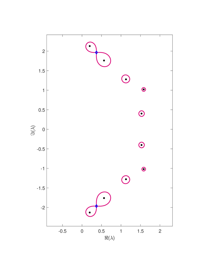
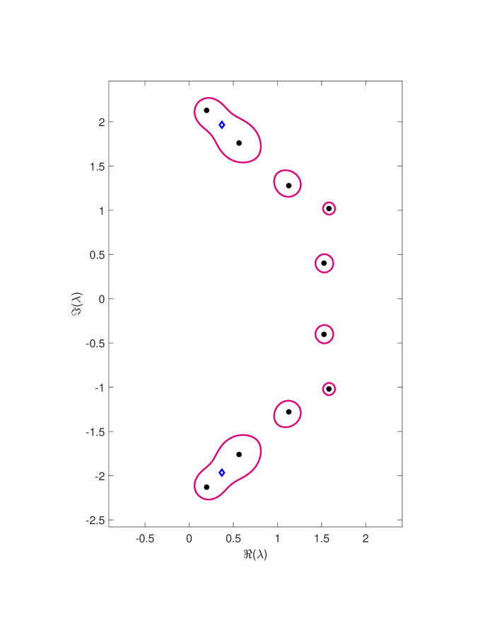
Fig. 3.1: Left picture: unstructured $\varepsilon$-pseudospectrum of the matrix (3.27) at the smallest value $\varepsilon=\varepsilon_{1}$ of coalescence of a pair of eigenvalues. Right picture: unstructured $\varepsilon$-pseudospectrum of the matrix (3.27) at the value $\varepsilon=\varepsilon_{2}$ corresponding to the norm of the smallest real perturbation of $A$ determining the coalescence of a pair of eigenvalues.

Considering unstructured perturbations to $A$, the smallest value $\varepsilon$ such that there exists a matrix $\Delta$ of norm $\varepsilon$ such that $A+\Delta$ has a defective pair of eigenvalues is $\varepsilon_{1}=0.035369524182688$. The corresponding $\varepsilon$-pseudospectrum with the two pairs of defective eigenvalues (represented by diamond symbols) is plotted in Figure 3.1 (left picture).

Considering instead real-structured perturbations to $A$, the smallest value $\varepsilon$ such that there exists a matrix $\Delta$ of norm $\varepsilon$ such that $A+\Delta$ has a defective pair of eigenvalues is $\varepsilon_{2}=0.050181307568931$. The corresponding $\varepsilon$-pseudospectrum with the two pairs of defective eigenvalues (represented by diamond symbols) is plotted in Figure 3.1 (right picture).

It is interesting to observe that the pairs of coalescent eigenvalues determined in the complex case, that is associated to the smallest complex perturbation of $A$, are

$$\lambda_{1,2}^{\mathbb{C}}=0.370080\ldots\pm 1.96544\ldots\mathrm{i}.$$

On the other side, the two (complex conjugate) pairs of coalescent eigenvalues determined in the real case, associated with the smallest real perturbation of $A$, are

$$\lambda^{\mathbb{R}}_{1,2}=0.370507\ldots\pm 1.965474\ldots\mathrm{i}.$$

This indicates that although the values of $\varepsilon_{1}$ and $\varepsilon_{2}$ are not very close, the points of coalescence of the eigenvalues are much closer.

VI.4 Nearest singular matrix pencil

VI.4.1 Problem setting

Let $A$ and $B$ be complex $n\times n$ matrices. The matrix pencil $\{A-\mu B\,:\,\mu\in\mathbb{C}\}$, or equivalently the pair $(A,B)$, is called singular if

$$A-\mu B\ \text{ is singular for all }\mu\in\mathbb{C}.$$ (4.1)

This notion is fundamental in the theory of linear differential-algebraic equations $B\dot{y}(t)=Ay(t)+f(t)$. If and only if the matrix pencil $(A,B)$ is singular, then there exists no initial value $y(0)$ such that the corresponding initial value problem has a unique solution.

A necessary condition for $(A,B)$ to be singular is clearly that both $A$ and $B$ are singular matrices (i.e. non-invertible). A sufficient condition for $(A,B)$ to be singular is that $A$ and $B$ have a common nonzero vector in their null-spaces. While this is a special case of particular interest, the Kronecker normal form of a matrix pencil (see Gantmacher, ?) shows that a common null-vector is not a necessary condition for a matrix pencil to be singular.

Given a matrix pencil $(A,B)$ that is not singular, it is of interest to know how far it is from a singular matrix pencil. In this section we fix $B$, which is assumed to be a singular matrix, and consider structured perturbations $\Delta A\in\mathcal{S}$ to $A$, where the structure space $\mathcal{S}$ is $\mathbb{C}^{n,n}$ or $\mathbb{R}^{n,n}$ or an arbitrary complex- or real-linear subspace, as considered in Section V.2. For example, $\mathcal{S}$ might be a space of real matrices with a given sparsity pattern. We consider the following two structured matrix nearness problems:

Problem 1.  Find $\Delta A\in\mathcal{S}$ of minimal Frobenius norm such that $(A+\Delta A,B)$ is a singular matrix pencil.

Problem 2.  Find $\Delta A\in\mathcal{S}$ of minimal Frobenius norm such that $A+\Delta A$ and $B$ have a common nonzero vector in their null-spaces.

If $A$ itself is also in $\mathcal{S}$, then both problems have a solution, because the trivial choice $\Delta A=-A$ gives us the singular matrix pencil $(0,B)$ and because the set of perturbations $\Delta A$ yielding singular matrix pencils $(A+\Delta A,B)$ is closed.

We will approach both problems by a two-level method in the spirit of Chapter IV. We extend the approach of Section V.8, which does not require computing eigenvalues and eigenvectors, or singular values and singular vectors, in the iterations.

We note that this approach would equally allow us to treat analogous matrix nearness problems where also $B$ is perturbed, but for ease of presentation we have chosen not to do so here. Moreover, in the applications of interest to dynamical systems on networks, $B$ is typically an adjacency matrix or related fixed matrix depending only on the network topology and hence is not subject to perturbations.

VI.4.2 Distance to structured singular matrix pencils

Given $n+1$ distinct complex numbers $\mu_{0},\dots,\mu_{n}$, the fundamental theorem of algebra together with the fact that a matrix is singular if and only if its determinant vanishes, shows that a matrix pencil $(A,B)$ is singular if and only if

$$\text{the $n+1$ matrices }\ A-\mu_{k}B\ \text{ are singular for }k=0,\dots,n.$$ (4.2)

Our numerical approach for Problem 1 is based on this criterion. The choice of the numbers $\mu_{0},\dots,\mu_{n}$ did not appear to be a critical issue in our numerical experiments. We had good experience with the choice $\mu_{k}=re^{2\pi k\mathrm{i}/(n+1)}$ of modulus $r=\|A\|_{F}/\|B\|_{F}$.

We proceed in analogy to Section V.8.2, working with matrix–vector products instead of eigenvalues or singular values. For $\varepsilon>0$ we introduce the functional $F_{\varepsilon}$ (of matrices $E\in\mathcal{S}$ of unit Frobenius norm and vectors $u_{k},v_{k}\in\mathbb{C}^{n}$ of unit Euclidean norm for $k=0,\dots,n$) in the following way: with $M_{k}=A-\mu_{k}B$,

$$F_{\varepsilon}(E,u_{0},\dots,u_{n},v_{0},\dots,v_{n})=\mbox{$\displaystyle{1\over 2}$}\sum_{k=0}^{n}\Bigl{(}\|u_{k}^{*}(M_{k}+\varepsilon E)\|^{2}+\|(M_{k}+\varepsilon E)v_{k}\|^{2}\Bigr{)}.$$ (4.3)

We follow the two-level approach of Chapter IV:

• Inner iteration: Given $\varepsilon>0$, we aim to compute a minimum of $F_{\varepsilon}$. We denote the minimum as $(E(\varepsilon),u_{0}(\varepsilon),\dots,u_{n}(\varepsilon),v_{0}(\varepsilon),\dots,v_{n}(\varepsilon))$.

• Outer iteration: We compute the smallest positive value $\varepsilon_{\star}$ with

  $$\phi(\varepsilon_{\star})=0,$$ (4.4)

  where $\phi(\varepsilon)$ is the minimal value of $F_{\varepsilon}$.

Provided that these computations succeed, we then have that $\Delta A_{\star}=\varepsilon_{\star}E(\varepsilon_{\star})\in\mathcal{S}$ is a solution to Problem 1 above, and $\varepsilon_{\star}$ is the distance of the matrix pencil $(A,B)$ to the set of structured singular matrix pencils of the form $(A+\Delta A,B)$ with $\Delta A\in\mathcal{S}$.

VI.4.3 Constrained gradient flow for the inner iteration

We closely follow the programme of Section V.8.2.

Structured gradient.

Consider a smooth path of structured matrices $E(t)\in\mathcal{S}$ and vectors $u_{k}(t),v_{k}(t)\in\mathbb{C}^{n}$ $(k=0,\dots,n+1)$. Since then also $\dot{E}(t)\in\mathcal{S}$, we have, similarly to (V.8.2),

$$\frac{d}{dt}\,F_{\varepsilon}(E(t),u_{0}(t),\dots,u_{n}(t),v_{0}(t),\dots,v_{n}(t))={\mbox{\rm Re}}\langle G,\varepsilon\dot{E}\rangle$$ (4.5)

$$+\ \sum_{k=0}^{n}\Bigl{(}{\mbox{\rm Re}}\langle(M_{k}+\varepsilon E)(M_{k}+\varepsilon E)^{*}u_{k},\dot{u}_{k}\rangle+\,{\mbox{\rm Re}}\langle(M_{k}+\varepsilon E)^{*}(M_{k}+\varepsilon E)v_{k},\dot{v}_{k}\rangle\!\Bigr{)}$$

with the structured gradient matrix

$$G=G_{\varepsilon}^{\mathcal{S}}(E,u_{0},\dots,u_{n},v_{0},\dots,v_{n})=\Pi^{\mathcal{S}}\sum_{k=0}^{n}\bigl{(}u_{k}u_{k}^{*}(M_{k}+\varepsilon E)+(M_{k}+\varepsilon E)v_{k}v_{k}^{*}\bigr{)},$$

where $\Pi^{\mathcal{S}}$ is again the orthogonal projection onto $\mathcal{S}$; see Section V.2.

Norm- and structure-constrained gradient flow.

Taking the norm constraints into account, we arrive at the following system of differential equations; cf. (V.8.3):

$$\varepsilon\dot{E} =-G+{\mbox{\rm Re}}\,\langle G,E\rangle\,E$$

$$\alpha_{k}\,\dot{u}_{k} =-(M_{k}+\varepsilon E)(M_{k}+\varepsilon E)^{*}u_{k}+\|(M_{k}+\varepsilon E)^{*}u_{k}\|^{2}\,u_{k}$$ (4.6)

$$\beta_{k}\,\dot{v}_{k} =-(M_{k}+\varepsilon E)^{*}(M_{k}+\varepsilon E)v_{k}+\|(M_{k}+\varepsilon E)v_{k}\|^{2}\,v_{k},$$

with scaling factors $\alpha_{k}(t)>0$ and $\beta_{k}(t)>0$, which we propose to choose as $\alpha_{k}=\|(M_{k}+\varepsilon E)^{*}u_{k}\|$ and $\beta_{k}=\|(M_{k}+\varepsilon E)v_{k}\|$ to obtain similar rates of change in $\varepsilon E$, $u_{k}$, $v_{k}$ near a stationary point.

By construction, the Frobenius norm 1 of $E(t)$ and the Euclidean norm 1 of $u_{k}(t)$ and $v_{k}(t)$ are preserved, and the functional $F_{\varepsilon}$ decays monotonically along solutions.

Stationary points.

At stationary points $(E,u_{0},\ldots,u_{n},v_{1},\ldots,v_{n})$ we find that $u_{k}$ and $v_{k}$ are left and right singular vectors to $M_{k}+\varepsilon E$, respectively, after rescaling $v_{k}\to{\rm e}^{\mathrm{i}\theta}v_{k}$ such that $\sigma_{k}=u_{k}^{*}(M_{k}+\varepsilon E)v_{k}$ is real and positive. When we arrive at the stationary point by the gradient flow (4.6), we can expect that the singular value $\sigma_{k}$ is the smallest singular value of $M_{k}$, since other stationary points are not stable.

In the stationary point we have $\sigma_{k}u_{k}=(M_{k}+\varepsilon E)v_{k}$ and $\sigma_{k}v_{k}=(M_{k}+\varepsilon E)^{*}u_{k}$ and hence the functional and the gradient are

$$F_{\varepsilon}=\sum_{k=0}^{n}\sigma_{k}^{2}\quad\text{ and }\quad G=\Pi^{\mathcal{S}}\sum_{k=0}^{n}2\sigma_{k}u_{k}v_{k}^{*}.$$ (4.7)

If $G\neq 0$ in the stationary point, it follows that $E$ is a real multiple of $G$. However, in contrast to Section V.2.3, this now does not imply that non-degenerate optimizers are projections of rank-1 matrices onto the structure space $\mathcal{S}$, because $G$ is no longer a projected rank-1 matrix. So we cannot work with rank-1 matrices here. In the inner iteration we therefore follow the norm- and structure-constrained gradient flow (4.6) into a stationary point.

VI.4.4 Outer iteration

We proceed as in Section IV.1.5. Under a differentiability assumption and under the assumption that the gradient $G(\varepsilon)=G_{\varepsilon}^{\mathcal{S}}$ is nonzero in the minimum of $F_{\varepsilon}$, we find in the same way as in Theorem IV.IV.1.4 a simple expression for the derivative of $\phi(\varepsilon)=\min F_{\varepsilon}$, which here again becomes (with ${}^{\prime}=d/d\varepsilon$)

$$\phi^{\prime}(\varepsilon)=-\|G(\varepsilon)\|_{F}<0.$$ (4.8)

This expression can be used in a Newton–bisection method. In view of (4.7), $\phi(\varepsilon)$ can be expected to behave asymptotically for $\varepsilon\nearrow\varepsilon_{\star}$ as

$$\phi(\varepsilon)\approx c\,(\varepsilon_{\star}-\varepsilon)^{2}.$$

The unknown quantities $c$ and $\varepsilon_{\star}$ can be estimated using $\phi(\varepsilon)$ and $\phi^{\prime}(\varepsilon)$, which is known from (4.8) for $\varepsilon<\varepsilon_{\star}$. This gives

$$\varepsilon_{\star}\approx\varepsilon-2\frac{\phi(\varepsilon)}{\phi^{\prime}(\varepsilon)},\qquad c\approx\frac{\phi^{\prime}(\varepsilon)^{2}}{4\phi(\varepsilon)}.$$

For $\varepsilon=\varepsilon_{k}<\varepsilon_{\star}$, we thus obtain the Newton-type iteration

$$\varepsilon_{k+1}=\varepsilon_{k}-2\frac{\phi(\varepsilon_{k})}{\phi^{\prime}(\varepsilon_{k})},$$ (4.9)

which yields a locally quadratically convergent iteration from the left (if instead $\varepsilon_{k}>\varepsilon_{\star}$ occurs, then we should use bisection, which would give a linear reduction of the error from the right).

VI.4.5 Distance to singular pencils with common null-vectors

We aim to find a perturbation $\Delta A\in\mathcal{S}$ of minimal Frobenius norm such that there exists a nonzero vector $v$ that is in the null-spaces of both $A+\Delta A$ and $B$. In the unstructured real or complex case ($\mathcal{S}=\mathbb{C}^{n,n}$ or $\mathbb{R}^{n,n}$), this problem is solved directly by computing the singular value decompositions $B=U_{B}\Sigma_{B}V_{B}^{*}$ and $U_{B}^{*}AV_{B}=U\Sigma V^{*}$ and taking the rank-1 perturbation $\Delta=-\sigma_{n}U_{B}u_{n}v_{n}^{*}V_{B}^{*}$.

To deal with the structured problem we introduce, for $\varepsilon>0$, a functional $F_{\varepsilon}$ (of matrices $E\in\mathcal{S}$ of unit Frobenius norm and a vector $v$ of unit Euclidean norm) as follows: With $\alpha=\|A\|_{2}$ and $\beta=\|B\|_{2}$, we set

$$F_{\varepsilon}(E,v)=\mbox{$\displaystyle{1\over 2\alpha^{2}}$}\|(A+\varepsilon E)v\|^{2}+\mbox{$\displaystyle{1\over 2\beta^{2}}$}\|Bv\|_{2}^{2}.$$ (4.10)

With this functional we again follow the two-level approach of Chapter IV. Provided that these computations succeed, we then have that $\Delta A_{\star}=\varepsilon_{\star}E(\varepsilon_{\star})\in\mathcal{S}$ is a solution to Problem 2 above, and $\varepsilon_{\star}$ is the distance of the matrix pencil $(A,B)$ to the set of matrix pencils of the form $(A+\Delta A,B)$ with $\Delta A\in\mathcal{S}$ for which $A+\Delta A$ and $B$ have a common nonzero null-vector.

The structured gradient is obtained by a straightforward calculation: For a path $E(t)\in\mathcal{S}$ and and $v(t)\in\mathbb{C}^{n}$, we have

$$\frac{d}{dt}F_{\varepsilon}(E(t),v(t))={\mbox{\rm Re}}\langle G,\varepsilon\dot{E}\rangle+{\mbox{\rm Re}}\langle g,\dot{v}\rangle,$$

with the projected rank-1 matrix

$$G=G_{\varepsilon}^{\mathcal{S}}(E,v)=\Pi^{\mathcal{S}}\Bigl{(}\mbox{$\displaystyle{1\over\alpha^{2}}$}\,(A+\varepsilon E)^{*}(A+\varepsilon E)vv^{*}\Bigr{)}$$

and the vector

$$g=g_{\varepsilon}(E,v)=\Bigl{(}\mbox{$\displaystyle{1\over\alpha^{2}}$}(A+\varepsilon E)^{*}(A+\varepsilon E)+\mbox{$\displaystyle{1\over\beta^{2}}$}B^{*}B\Bigr{)}v.$$

With this structured gradient, the full programme of Section V.2 carries over to the present situation, including the rank-1 matrix differential equation (V.2.10) and its discretization, which were not available for the (full-rank) gradient of Section VI.4.3.

For the outer iteration, we again use a Newton–bisection method in the same way as in Section VI.4.4. Here we have again $\phi^{\prime}(\varepsilon)=-\|G(\varepsilon)\|_{F}$ with $G(\varepsilon)=G_{\varepsilon}^{\mathcal{S}}(E(\varepsilon),v(\varepsilon))$.

This approach extends directly to the case when also $B$ can be perturbed. The only reason why we have not done so here, is that the notation would be more complicated, requiring two perturbations $E_{A}\in\mathcal{S}_{A}$ and $E_{B}\in\mathcal{S}_{B}$ and the squared perturbation size $\varepsilon^{2}=\varepsilon_{A}^{2}+\varepsilon_{B}^{2}$.

VI.5 Stability radii for delay differential equations

VI.5.1 A simple example

Consider the scalar delay differential equation

$$\dot{x}(t)=ax(t)+bx(t-1)$$ (5.1)

with $a,b\in\mathbb{R}$. Looking for solutions $x(t)=c{\rm e}^{\lambda t}$ gives the characteristic equation

$$\lambda-a-b\,{\rm e}^{-\lambda}=0.$$ (5.2)

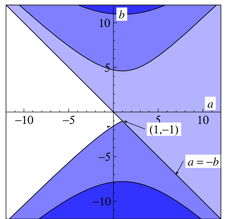
Fig. 5.1: Region of the $(a,b)$-real plane such that the solution of (5.1) is asymptotically stable (white set in the right illustration).

A main feature of this problem is that the entire function $\lambda-a-b\,{\rm e}^{-\lambda}$ has infinitely many roots and stability can be proved if and only if all the roots lie on the complex left-plane or - in other words - the rightmost root has negative real part. This is what happens when $a=0.5,b=-1$ as shown in Figure 5.1 (left illustration).

The stability of a linear system of delay equations

$$\dot{x}(t) = A_{1}x(t)+A_{2}x\left(t-\tau\right),\qquad t>0$$ (5.3)

$$x(t) = g(t),\qquad t\in\left[-\tau,0\right]$$

with $A_{1},A_{2}$ given $n\times n$ matrices and $\tau>0$ a constant delay, can be analyzed in a similar way.

Inserting solutions of the form $x(t)=v\,{\rm e}^{\lambda t}$ (with nonzero $v\in\mathbb{C}^{n}$) we get

$$\left(\lambda\mathrm{I}-A_{1}-A_{2}{\rm e}^{-\lambda\tau}\right)v=0,$$ (5.4)

which is a nonlinear eigenvalue problem.

It is known that if the infinitely many eigenvalues strictly lie within the complex left half-plane, then every solution of (5.3) is asymptotically stable, independently of the initial data.

The main difficulty here is that in general the matrices $A_{1}$ and $A_{2}$ do not commute, so that they cannot be transformed simultaneously to diagonal form, in contrast to the case of linear ordinary differential equations. Suitable algorithms for the numerical computation of characteristic roots of linear delay systems are available; see e.g. Engelborghs and Roose, 2002, Breda, Maset and Vermiglio, 2005, Jarlebring, Meerbergen and Michiels, 2010 (based on Krylov solvers).

VI.5.2 Nonlinear eigenvalue problem and stability radius

Nonlinear eigenvalue problem.

We consider the problem of determining the eigenvalues $\lambda\in\mathbb{C}$ and corresponding eigenvectors $v\in\mathbb{C}^{n}\setminus\{0\}$ that satisfy

$$\left(\sum_{i=0}^{m}f_{i}(\lambda)A_{i}\right)v=0,$$ (5.5)

where $A_{0},\ldots,A_{m}$ are given $n\times n$ matrices and the functions $f_{0},\ldots,f_{m}$ are entire complex functions with

$$f_{i}(\overline{\lambda})=\overline{f_{i}(\lambda)},\qquad 0\leq i\leq m.$$

We again denote the spectrum by $\Lambda$, i.e.

$$\Lambda:=\left\{\lambda\in\mathbb{C}:\ \sum_{i=0}^{m}f_{i}(\lambda)A_{i}\ \text{ is a singular matrix}\right\}$$ (5.6)

Perturbed nonlinear eigenvalue problem.

We are interested in the effect of bounded perturbations $\Delta A_{i}$ of $A_{i}$, which are allowed to be complex. We consider the perturbed eigenvalues $\widetilde{\lambda}$ with

$$\left(\sum_{i=0}^{m}f_{i}(\widetilde{\lambda})(A_{i}+\Delta A_{i})\right)\widetilde{v}=0$$ (5.7)

for some $\widetilde{v}\neq 0$. We let

$$\Delta=\left(\Delta A_{0},\dots,\Delta A_{m}\right).$$

Introducing weights $w_{i}>0$ for $i=0,\ldots,m$, we make use of the weighted norm

$$\|\Delta\|_{w}:=\sqrt{\sum\limits_{i=0}^{m}w_{i}^{2}\|\Delta A_{i}\|_{F}^{2}}$$

We consider perturbations bounded as

$$\|\Delta\|_{w}\leq\varepsilon.$$

Taking $w_{i}=+\infty$ means that the matrix $A_{i}$ is not perturbed.

Pseudospectra and stability radius.

The $\varepsilon$-pseudospectrum is the complex set

$$\Lambda_{\varepsilon}=\bigcup\limits_{\|\Delta\|_{w}\leq\varepsilon}\left\{\lambda\in\mathbb{C}:\ \sum_{i=0}^{m}f_{i}(\lambda)(A_{i}+\Delta A_{i})\ \text{ is a singular matrix}\right\},$$

that is, the set of eigenvalues associated with all perturbed problems having $\|\Delta\|_{w}\leq\varepsilon$.

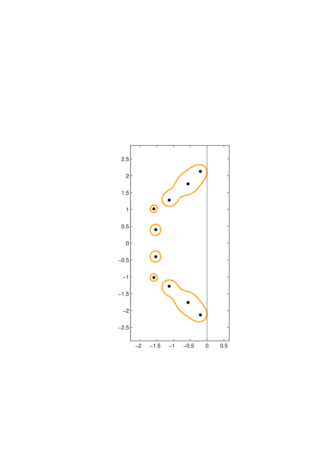
Fig. 5.2: Rightmost roots of an example of system (5.4) and $\varepsilon$-pseudospectrum tangential to the imaginary axis (showing $\varepsilon=\varepsilon_{\star}$).

The $\varepsilon$-pseudospectral abscissa is defined as

$$\alpha_{\varepsilon}:=\sup\left\{{\mbox{\rm Re}}\,\lambda\,:\,\lambda\in\Lambda_{\varepsilon}\right\},$$ (5.8)

where in this case – because of the infinitely many eigenvalues – the $\max$ is replaced by the $\sup$.

Asymptotic stability is associated with the requirement that the spectrum be located in the open left half-plane and bounded away from the imaginary axis. The stability radius (or distance to instability) of an asymptotically stable system is defined as

$$\varepsilon_{\star}:=\inf\left\{\varepsilon>0:\ \alpha_{\varepsilon}\geq 0\right\}.$$

Problem. Compute the stability radius $\varepsilon_{\star}$ for the nonlinear eigenvalue problem (5.7).

Assumptions.

For nonlinear eigenvalue problems the pseudospectral abscissa may be equal to infinity (as in differential-algebraic equations), or a globally rightmost point of the pseudospectrum may not exist. To exclude such cases, we assume the following:

• For every $\varepsilon>0$,  $\alpha_{\varepsilon}<+\infty$.

• There exists $r>0$ such that the set $\Lambda_{\varepsilon_{\star}}\cap\{\lambda\in\mathbb{C}:\ {\mbox{\rm Re}}\,\lambda\geq-r\}$ is bounded.

As an example which does not fulfill assumption (ii), consider the following neutral equation

$$\dot{x}(t)=\dot{x}(t-\tau)-2x(t)-x(t-\tau).$$ (5.9)

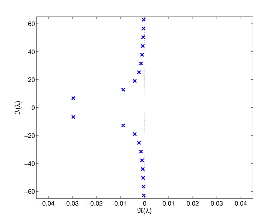
Fig. 5.3: Rightmost roots of the neutral equation.

Its characteristic equation is given by

$$\lambda\left(1-{\rm e}^{-\lambda}\right)+2+{\rm e}^{-\lambda}=0,$$

which has a sequence of roots approaching the imaginary axis with increasing imaginary part. Here the spectral abscissa is equal to zero, yet there is no characteristic root with zero real part.

VI.5.3 Two-level approach

We use a two-level approach as in previous sections to compute the stability radius $\varepsilon_{\star}$. We assume (5.5) fulfils assumptions (i) and (ii). Moreover we also assume that $w_{i}<\infty$ for $i=0,\ldots,m$ (otherwise the matrices associated to infinite weights are not perturbed). We write perturbations as

$$\Delta A_{i}=\varepsilon E_{i},\qquad i=0,\dots,m$$

with

$$\|(E_{0},\dots,E_{m})\|_{w}^{2}=\sum_{i=0}^{m}w_{i}^{2}\|E_{i}\|_{F}^{2}=1.$$

We denote by $\mathcal{S}_{w}^{1}$ the unit ball for the weighted norm $\|\cdot\|_{w}$. We look for

$$\alpha_{\varepsilon}=\max\limits_{(E_{0},\ldots,E_{m})\in\mathcal{S}_{w}^{1}}\biggl{\{}{\mbox{\rm Re}}\,\lambda:\ \sum_{i=0}^{m}f_{i}(\lambda)(A_{i}+\varepsilon E_{i})\ \text{ is a singular matrix}\biggr{\}}.$$

We introduce the functional

$$F_{\varepsilon}\left(E_{0},E_{1},\ldots,E_{m}\right)=-{\mbox{\rm Re}}\,\lambda,$$ (5.10)

where $\lambda$ is the rightmost eigenvalue of the nonlinear eigenvalue problem (5.7) with $\Delta A_{i}=\varepsilon E_{i}$. We again follow the two-level approach of Chapter IV:

• Inner iteration: Given $\varepsilon>0$, we aim to compute $(m+1)$-tuples of complex $n\times n$ matrices $\bigl{(}E_{0}(\varepsilon),\dots,E_{m}(\varepsilon)\bigr{)}\in\mathcal{S}_{w}^{1}$ that minimize $F_{\varepsilon}$:

  $$\bigl{(}E_{0}(\varepsilon),\dots,E_{m}(\varepsilon)\bigr{)}=\arg\min\limits_{(E_{0},E_{1},\ \ldots,E_{m})\in\mathcal{S}_{w}^{1}}F_{\varepsilon}\left(E_{0},E_{1},\ldots,E_{m}\right).$$ (5.11)

• Outer iteration: We compute the smallest positive value $\varepsilon_{\star}$ with

  $$\phi(\varepsilon_{\star})=0,$$ (5.12)

  where $\phi(\varepsilon)=F_{\varepsilon}(E_{0}(\varepsilon),\dots,E_{m}(\varepsilon))=-\alpha_{\varepsilon}$. Then, $\varepsilon_{\star}$ is the stability radius.

VI.5.4 Inner iteration: Rank-1 dynamics

The programme of Chapter II extends to the current situation as follows.

Free gradient.

We consider a path $\bigl{(}E_{0}(t),\dots,E_{m}(t)\bigr{)}\in\mathcal{S}_{w}^{1}$ for $t$ in an open interval around $t_{0}$ and we assume that the path of eigenvalues $\lambda(t)$ with

$$\det\bigl{(}f_{0}(\lambda(t))(A_{0}+\varepsilon E_{0}(t))+\ldots+f_{m}(\lambda(t))(A_{m}+\varepsilon E_{m}(t))\bigr{)}=0$$

consists of simple eigenvalues. As in Lemma II.II.2.1, we find that

$$\frac{1}{\varepsilon\kappa(t)}\,\frac{d}{dt}F_{\varepsilon}(E_{0}(t),\dots,E_{m}(t))=\sum_{i=0}^{m}w_{i}^{2}\,{\mbox{\rm Re}}\bigl{\langle}G_{i}(E_{0}(t),\dots,E_{m}(t)),\dot{E}_{i}(t)\bigr{\rangle}$$ (5.13)

with the rescaled partial gradient

$$G_{i}\left(E_{0},E_{1},\ldots,E_{m}\right)=-w_{i}^{-2}f_{i}(\overline{\lambda})xy^{*},\qquad i=0,\dots,m,$$ (5.14)

where $x$ and $y$ are left and right eigenvectors corresponding to $\lambda$, chosen of unit norm and with positive inner product, and where $\kappa=1/(x^{*}y)$.

Norm-constrained gradient flow.

We consider the gradient flow on the unit sphere $\mathcal{S}_{w}^{1}$,

$$\dot{E}_{i}=-G_{i}(E_{0},\dots,E_{m})+\mu E_{i},\qquad i=0,\dots,m,$$ (5.15)

with the Lagrange multiplier

$$\mu=\sum_{i=0}^{m}w_{i}^{2}\,{\mbox{\rm Re}}\langle G_{i}(E_{0},\dots,E_{m}),E_{i}\rangle.$$

This ensures that for $(E_{0},\dots,E_{m})\in\mathcal{S}_{w}^{1}$,

$$\frac{1}{2}\,\frac{d}{dt}\|(E_{0},\dots,E_{m})\|_{w}^{2}=\sum_{i=1}w_{i}^{2}\,{\mbox{\rm Re}}\langle\dot{E}_{i},E_{i}\rangle=0,$$

so that the weighted norm 1 is preserved along the flow.

Monotonicity.

Assuming simple eigenvalues along the trajectory, we again obtain the monotonicity property as in Theorem II.II.2.3,

$$\frac{d}{dt}F_{\varepsilon}(E_{0}(t),\dots,E_{m}(t))=-\varepsilon\kappa\sum_{i=0}^{m}w_{i}^{2}\|G_{i}(E_{0},\dots,E_{m})-\mu E_{i}\|_{F}^{2}\leq 0.$$ (5.16)

Stationary points.

Also the characterization of stationary points as given in Theorem II.II.2.3 extends with the same proof: Let $\varepsilon>0$ be fixed and let $(E_{0},\dots,E_{m})\in\mathcal{S}_{w}^{1}$ be such that the correponding rightmost eigenvalue $\lambda$ is simple and $G_{i}(E_{0},\dots,E_{m})\neq 0$ for $i=0,\dots,m$. Then,

$$(E_{0},\dots,E_{m})$$ is a stationary point of the differential equation (5.15) if and only if (5.17)

$$E_{i} G_{i}(E_{0},\dots,E_{m}) i=0,\dots,m$$ is the same real multiple of for .

In particular, this shows that at non-degenerate stationary points, $E_{i}$ is of rank 1 for $i=0,\dots,m$.

Rank-$1$ constrained gradient flow.

In view of the rank-1 property of optimizers, we proceed further as in Chapter II and constrain the gradient flow (5.15) to the rank-$1$ manifold $\mathcal{M}_{1}$ by projecting the right-hand side onto the tangent space. This yields the norm- and rank-1 constrained gradient flow

$$\dot{E}_{i}=-P_{E_{i}}G_{i}+\mu E_{i},\qquad i=0,\dots,m$$ (5.18)

with $E_{i}=\sigma_{i}u_{i}v_{i}^{*}$ of rank $1$ with $\|u_{i}\|=\|v_{i}\|=1$ for all $i$, with $P_{E_{i}}$ the orthogonal projection onto the tangent space at $E_{i}\in\mathcal{M}_{1}$, and the Lagrange multiplier $\mu$ as in (5.15).

Similarly to the prototype case considered in Chapter II, it can be shown that the rank-1 projected differential equations preserve norm, monotonicity and stationary points. The differential equations are integrated numerically into a stationary point in the way described in Chapter II, working with the vectors that define the rank-1 matrices $E_{i}$ and advancing them in time by a splitting method. This again yields a significant reduction in CPU time and memory.

VI.5.5 Outer iteration

We use again a mixed Newton–bisection method to compute the stability radius, which is the smallest zero $\varepsilon_{\star}$ of $\phi(\varepsilon)=F_{\varepsilon}(E_{0}(\varepsilon),\dots,E_{m}(\varepsilon))$. Under assumptions analogous to Chapter IV, we find in the same way that $\phi$ is continuously differentiable and the derivative here becomes, with ${}^{\prime}=d/d\varepsilon$ and $G_{i}(\varepsilon)=G_{i}^{\varepsilon}(E_{0}(\varepsilon),\dots,E_{m}(\varepsilon))$ and $\kappa(\varepsilon)=1/(x(\varepsilon)^{*}y(\varepsilon))>0$,

$$\phi^{\prime}(\varepsilon)=-\kappa(\varepsilon)\,\|(G_{0}(\varepsilon),\dots,G_{m}(\varepsilon))\|_{w}<0,$$ (5.19)

which is used in the Newton-based iteration.

VI.5.6 Numerical examples

A linear system of delay differential equations.

Consider the linear system of delay equations

$$A_{0}\dot{x}(t) = A_{1}x(t)+A_{2}x\left(t-1\right),\qquad t>0$$ (5.20)

$$x(t) = g(t),\qquad t\in\left[-\tau,0\right]$$

with $A_{0},A_{1},A_{2}$ given $n\times n$ matrices and the delay $\tau=1$.

It is possible to prove that if $A_{0}$ is nonsingular, (5.20) fulfils assumptions (i) and (ii).

The associated nonlinear eigenvalue problem is given by

$$\det\left(\lambda A_{0}-A_{1}-A_{2}{\rm e}^{-\lambda}\right)=0,$$ (5.21)

so that - in the considered setting - $f_{0}(\lambda)=\lambda,\ f_{1}(\lambda)=-1,\ f_{2}(\lambda)=-{\rm e}^{-\lambda}.$

We set $A_{0}=\mathrm{I}$ and $w_{0}=\infty$ implying this way the identity matrix $A_{0}$ is not perturbed. This gives us a constrained gradient system (5.15) or (5.18)) with matrices $E_{1}$ and $E_{2}$. Note that $E_{0}$ is missing because $w_{0}=+\infty$.

A partial differential equation with a delay.

Consider the problem (Jarlebring et al., 2010)

$$\frac{\partial v(x,t)}{\partial t}=\frac{\partial^{2}v(x,t)}{\partial x^{2}}+a_{0}(x)v(x,t)+a_{1}(x)v(\pi-x,t-1),$$ (5.22)

where $a_{0}(x)=-2\sin(x)$, $a_{1}(x)=2\sin(x)$, $v_{x}(0,t)=v_{x}(\pi,t)=0$.

Space derivatives are approximated by central differences. This gives a delay eigenvalue problem of the form (5.20) with sparse matrices $A_{0}$ and $A_{1}$. The dimension is chosen as $n=5000$. Computed pseudospectral abscissae corresponding to different weigths are shown in Table 5.1.

$\alpha$	$(w_{1},w_{2})$	$\varepsilon$	$\alpha_{\varepsilon}$	#steps
-3.312133337e-1	$(1/2,1/2)$	1.e-3	-3.297978515e-1	2
		1.e-2	-3.170982221e-1	3
		1.e-1	-1.937166436e-1	4
		1	8.647127140e-1	8
	(1/4,$\infty$)	1.e-3	-3.300292687e-1	2
		1.e-2	-3.193270916e-1	3
		1.e-1	-2.075848221e-1	4
		1	+1.641134830e00	10
	($\infty$,1/4)	1.e-3	-3.295667765e-1	2
		1.e-2	-3.149018637e-1	3
		1.e-1	-1.816328080e-1	4
		1	+5.599912563e-1	7

Table 5.1: Pseudospectral abscissa $\alpha_{\varepsilon}=-\phi(\varepsilon)$ for the delayed PDE problem.

VI.6 Kreiss number

The essential part of the Kreiss matrix theorem (Kreiss ?) in the sharp version of Spijker (?), conjectured by LeVeque & Trefethen (?), states that if an $n\times n$ complex matrix $A$ has a finite Kreiss number

$$K(A):=\sup_{\mathrm{Re}\,\lambda>0}\,{\mbox{\rm Re}}\,\lambda\ \|(A-\lambda I)^{-1}\|_{2}<\infty,$$ (6.1)

then its exponential is bounded by

$$K(A)\leq\sup_{t\geq 0}\|{\rm e}^{tA}\|_{2}\leq{\rm e}\,n\,K(A).$$ (6.2)

In this section we consider the following computational problem.

Problem. Given a matrix $A\in\mathbb{C}^{n,n}$ having all its eigenvalues in the open left complex half-plane, compute its Kreiss number $K(A)$.

Although this is not a matrix nearness problem, we include it in this chapter, because we will address it with variants of the techniques used for computing the $\varepsilon$-pseudospectral abscissa and the stability radius in Sections III.2 and IV.1. We will describe two such approaches, with emphasis on the second approach.

VI.6.1 Using pseudospectral abscissae

For $\varepsilon>0$ let $\alpha_{\varepsilon}(A)$ be the $\varepsilon$-pseudospectral abscissa of $A$ and $\varepsilon_{\star}$ with $\alpha_{\varepsilon_{\star}}(A)=0$ the stability radius. We recall formula (III.1.9), viz.,

$$\max_{\mathrm{Re}\,\lambda\geq\alpha_{\varepsilon}(A)}\|(A-\lambda I)^{-1}\|_{2}=\frac{1}{\varepsilon}.$$ (6.3)

Since the maximum is assumed for $\mathrm{Re}\,\lambda=\alpha_{\varepsilon}(A)$ by the maximum principle, this implies the following formula, which is given by Trefethen & Embree (?), p. 138.

• The Kreiss number is determined by the $\varepsilon$-pseudospectral abscissae for ${\varepsilon>\varepsilon_{\star}}$ as

  $$K(A)=\sup_{\varepsilon>\varepsilon_{\star}}\alpha_{\varepsilon}(A)\,\frac{1}{\varepsilon}.$$ (6.4)

  The pseudospectral abscissa $\alpha_{\varepsilon}(A)$ can be computed by the various methods described in Section III.2. It then remains to compute the supremum over $\varepsilon>\varepsilon_{\star}$ (or equivalently, over all $\varepsilon>0$). While $\alpha_{\varepsilon}(A)$ grows monotonically with $\varepsilon$, this does not imply that $\alpha_{\varepsilon}(A)/\varepsilon$ is a unimodal function of $A$, and little appears to be known about the location and number of local maxima of $\alpha_{\varepsilon}(A)/\varepsilon$.

VI.6.2 Using weighted pseudospectra

In an alternative approach, for a nonnegative weight function $w(\lambda)$, here in particular $w(\lambda)=\max({\mbox{\rm Re}}\,\lambda,0)$, we consider the weighted $\varepsilon$-pseudospectrum (for $\varepsilon>0$)

$$\Lambda_{\varepsilon}^{w}(A)=\left\{\lambda\in\mathbb{C}\setminus\Lambda(A)\,:\,w(\lambda)\,\|(A-\lambda I)^{-1}\|_{2}\geq\mbox{$\displaystyle{1\over\varepsilon}$}\right\}.$$

For $w(\lambda)=\max({\mbox{\rm Re}}\,\lambda,0)$ we note that $w(\lambda)\,\|(A-\lambda I)^{-1}\|_{2}$ is zero in the left complex half-plane, bounded in the right half-plane, and is bounded by 1 asymptotically for ${|\lambda|\to\infty}$. It follows that $\Lambda_{\varepsilon}^{w}(A)$ lies in the complex right half-plane or is empty, and $\Lambda_{\varepsilon}^{w}(A)$ is a bounded set for every $\varepsilon<1$. There exists $\varepsilon_{\star}^{w}>0$ such that

$$\Lambda_{\varepsilon}^{w}(A)=\emptyset\ \ \varepsilon<\varepsilon_{\star}^{w}\ \Lambda_{\varepsilon_{\star}^{w}}^{w}(A)\neq\emptyset$$ for  but  ,

that is, $\varepsilon_{\star}^{w}$ is the smallest $\varepsilon$ for which $\Lambda_{\varepsilon}^{w}(A)$ is not empty. This means that $1/\varepsilon_{\star}^{w}$ is the smallest upper bound of $w(\lambda)\,\|(A-\lambda I)^{-1}\|_{2}$ on the right half-plane and hence equals the Kreiss number $K(A)$. We restate this observation as a lemma.

• The Kreiss number is obtained as

  $$K(A)=\frac{1}{\varepsilon_{\star}^{w}}.$$ (6.5)

  We set out to compute $\varepsilon_{\star}^{w}$ using a characterization of $\Lambda_{\varepsilon}^{w}(A)$ in terms of eigenvalues of perturbed matrices. We have $\lambda\in\Lambda_{\varepsilon}^{w}(A)$ if and only if $\sigma_{\mathrm{min}}(A-\lambda I)\leq w(\lambda)\varepsilon$, and the proof of Theorem III.III.1.2 shows that this is equivalent to the existence of a rank-1 matrix $\Theta$ of 2-norm (or equivalently Frobenius norm) at most $w(\lambda)\varepsilon$ such that $A+\Theta-\lambda I$ is a singular matrix. Writing $\Theta=w(\lambda)\varepsilon E$ with $\|E\|_{F}=\|E\|_{2}\leq 1$, we thus obtain the characterization of $\Lambda_{\varepsilon}^{w}(A)$ via a nonlinear eigenvalue problem:

  $$\Lambda_{\varepsilon}^{w}(A)=\bigl{\{}\lambda\in\mathbb{C}\setminus\Lambda(A)\,:\, \text{ There exists $E$ with $\|E\|_{F}\leq 1$ such that}\bigr{.}$$

  . $$\text{ $A+w(\lambda)\varepsilon E-\lambda I$ is singular}\bigr{\}}.$$

  This characterization of $\Lambda_{\varepsilon}^{w}(A)$ allows us to reformulate the problem of finding $\varepsilon_{\star}^{w}=1/K(A)$.

  Problem (rephrased as a weighted matrix nearness problem). Given a matrix $A\in\mathbb{C}^{n,n}$ having all its eigenvalues in the open left complex half-plane, find $\lambda\in\mathbb{C}$ with ${\mbox{\rm Re}}\,\lambda\geq 0$ and $\Theta\in\mathbb{C}^{n,n}$ of minimal Frobenius norm such that $A+w(\lambda)\Theta-\lambda I$ is singular.

  Then we have $\|\Theta\|_{F}=\varepsilon_{\star}^{w}$ and hence $K(A)=1/\|\Theta\|_{F}$ if $w(\lambda)={\mbox{\rm Re}}\,\lambda$ for ${\mbox{\rm Re}}\,\lambda\geq 0$. On the other hand, in the unweighted case $w(\lambda)=1$ the above problem reduces to finding the stability radius of $A$ as $\varepsilon_{\star}=\|\Theta\|_{F}$.

We know that $K(A)\geq 1$ and are mainly interested in the case with strict inequality, which excludes normal matrices.

• $K(A)>1$. This implies that $\Lambda_{\varepsilon}^{w}(A)$ is a nonempty bounded set for $\varepsilon_{\star}^{w}\leq\varepsilon<1$. For such $\varepsilon$ we introduce the right and left weighted $\varepsilon$-pseudospectral abscissae

  $$\alpha_{\varepsilon}^{w}(A)=\max\{{\mbox{\rm Re}}\,\lambda\,:\,\lambda\in\Lambda_{\varepsilon}^{w}(A)\}<\infty,$$

  $$\beta_{\varepsilon}^{w}(A)=\min\ \{{\mbox{\rm Re}}\,\lambda\,:\,\lambda\in\Lambda_{\varepsilon}^{w}(A)\}>0.$$

  We have the weighted variants of (6.3),

  $$\max_{\mathrm{Re}\,\lambda\geq\alpha_{\varepsilon}^{w}(A)}w(\lambda)\,\|(A-\lambda I)^{-1}\|_{2}=\frac{1}{\varepsilon},$$

  $$\max_{\mathrm{Re}\,\lambda\leq\beta_{\varepsilon}^{w}(A)}w(\lambda)\,\|(A-\lambda I)^{-1}\|_{2}=\frac{1}{\varepsilon}.$$

  We now make the further assumption that all global maxima of $w(\lambda)\,\|(A-\lambda I)^{-1}\|_{2}$ have the same real part.

  • The set $\{{\mbox{\rm Re}}\,\lambda\,:\,{\mbox{\rm Re}}\,\lambda\ \|(A-\lambda I)^{-1}\|_{2}=K(A)\}$ consists of a single real number $\rho$. This implies that

    $$\lim_{\varepsilon\searrow\varepsilon_{\star}^{w}}\alpha_{\varepsilon}^{w}(A)=\lim_{\varepsilon\searrow\varepsilon_{\star}^{w}}\beta_{\varepsilon}^{w}(A)=\rho.$$

Two-level iteration.

To compute the Kreiss number $K(A)=1/\varepsilon_{\star}^{w}$, we use a two-level iteration that is very similar to that of Chapter IV.

• Inner iteration: For a given $\varepsilon$ with $\varepsilon_{\star}^{w}\leq\varepsilon<1$, we compute the right and left weighted $\varepsilon$-pseudospectral abscissae $\alpha_{\varepsilon}^{w}(A)$ and $\beta_{\varepsilon}^{w}(A)$, analogously to the computation of the $\varepsilon$-pseudospectral abscissa via a rank-1 gradient flow in Chapter II or the algorithms in Section III.2.

• Outer iteration: Given a tolerance parameter $\delta>0$, we compute $\varepsilon>\varepsilon_{\star}^{w}$ with

  $$\alpha_{\varepsilon}^{w}(A)-\beta_{\varepsilon}^{w}(A)\leq\delta,$$ (6.6)

  and we denote this $\varepsilon$ as $\varepsilon_{\delta}$. This can be done by a mixed Newton–bisection method as in Chapter IV. We then take $K_{\delta}(A)=1/\varepsilon_{\delta}$ as an approximation to $K(A)$.

The main difference to the two-level iteration for the stability radius in Chapter IV is that we now have to deal with nonlinear eigenvalue problems, where we need to compute eigenvalues $\lambda$ (and corresponding left and right eigenvectors) such that

$$A+w(\lambda)\varepsilon E-\lambda I\ \text{ is singular}.$$

In contrast to the situation considered in the preceding section, here $w$ is not a holomorphic function, and so algorithms for nonlinear eigenvalue problems with holomorphic functions, such as the method proposed by Beyn (?), cannot be applied. See Güttel & Tisseur (?) for a review of numerical methods for nonlinear eigenvalue problems. In the present case, when $\varepsilon<1$ (ideally $\varepsilon\ll 1$), we can do a (fast) converging iteration where the $(n+1)$st iterate $\lambda_{n+1}$ is determined as a rightmost eigenvalue of the perturbed matrix $A+w(\lambda_{n})\varepsilon E$.

Aside from this extra difficulty of dealing with a generalized eigenvalue problem, the whole programme of Chapters II and IV extends in a straightforward way to the present situation.

VI.6.3 Robustness under structured perturbations

So far we considered the Kreiss number of a single given matrix $A$. We now consider the Kreiss numbers of perturbed matrices $A+\Delta$ with (possibly) structured perturbations $\Delta\in\mathcal{S}$ bounded by $\|\Delta\|_{F}\leq\delta$ for a given $\delta>0$ and define the supremum of the Kreiss numbers of the collection of such perturbed matrices by

$$K_{\delta}^{\mathcal{S}}(A):=\sup_{\Delta\in\mathcal{S},\|\Delta\|_{F}\leq\delta}K(A+\Delta).$$

Letting

$$\varepsilon_{\delta}^{w,\mathcal{S}}=\min_{\Delta\in\mathcal{S},\|\Delta\|_{F}\leq\delta}\varepsilon_{\star}^{w}(A+\Delta)$$

with the weight function $w(\lambda)={\mbox{\rm Re}}\,\lambda$ for ${\mbox{\rm Re}}\,\lambda\geq 0$, we then have

$$K_{\delta}^{\mathcal{S}}(A)=\frac{1}{\varepsilon_{\delta}^{w,\mathcal{S}}}.$$

The problem of computing $K_{\delta}^{\mathcal{S}}(A)$ can thus be reformulated in the following way.

Problem (rephrased as a weighted matrix nearness problem). Given a matrix $A\in\mathbb{C}^{n,n}$ having all its eigenvalues in the open left complex half-plane, and given a structure space $\mathcal{S}\subset\mathbb{C}^{n,n}$ and $\delta>0$, determine $\varepsilon_{\delta}^{w,\mathcal{S}}$ as the smallest $\varepsilon>0$ for which there exist $\lambda\in\mathbb{C}$ with ${\mbox{\rm Re}}\,\lambda\geq 0$, $\Delta\in\mathcal{S}$ bounded by $\|\Delta\|_{F}\leq\delta$ and $\Theta\in\mathbb{C}^{n,n}$ bounded by $\|\Theta\|_{F}\leq\varepsilon$ such that $A+\Delta+w(\lambda)\Theta-\lambda I$ is singular.

In the unweighted case $w(\lambda)=1$ this problem reduces to finding the inverse common resolvent bound $\varepsilon_{\delta}^{\mathcal{S}}(A)$ studied in Section V.6. The weighted case considered here allows for an analogous algorithm. In particular, for the extremal perturbations we again find that $\Delta$ is proportional to $\Pi^{\mathcal{S}}\Theta$ and $\Theta$ is of rank 1, which enables us to reduce the problem to that of finding an optimal rank-1 perturbation matrix $\Theta$ as the stationary point of a rank-1 matrix differential equation. The computational cost for computing $K_{\delta}^{\mathcal{S}}(A)$ is then comparable to that for computing just $K(A)$ with the two-level algorithm of the previous subsection.

VI.7 Notes

Matrix stabilization.

Finding the smallest (complex, real or structured) stabilizing perturbation to a given matrix is a harder problem than the complementary problem of finding the smallest destabilizing perturbation as discussed in previous chapters. Several conceptually different algorithms for matrix stabilization with complex or real unstructured perturbations have been proposed in the literature.

A black-box approach is to consider the problem of finding the nearest stable matrix as a nonsmooth (but almost everywhere smooth), nonconvex, constrained optimization problem and apply general software for this class of problems, such as given by Curtis, Mitchell & Overton (?).

Orbandexivry, Nesterov & Van Dooren (?) presented a matrix stabilization algorithm that uses successive convex approximations. They started from Lyapunov’s characterization of stability to reformulate the matrix stabilization problem as finding complex $n\times n$ matrices $X$ and $P$ that give

$$\inf_{X,P}\tfrac{1}{2}\|X-A\|_{F}^{2}\quad\text{ such that $P=P^{*}$ and $XP+PX^{*}$ are both positive definite.}$$

This nonconvex optimization problem is related to the convex problem of finding, for given $X$ and $P$,

$$\inf_{H}\tfrac{1}{2}\|X+H-A\|_{F}^{2}\quad\text{ such that $H$ is in a suitable ellipsoid defined by $P$ and $X$}.$$

This update for $X$ is complemented with a procedure that associates an admissible $P$ to $X$. With an $O(n^{5})$ complexity per iteration, the algorithm is limited to small matrices.

Gillis & Sharma (?) showed that a real square matrix $A$ is stable if and only if it can be written as the matrix of a dissipative Hamiltonian system, i.e. $A=(J-R)Q$, where $J$ is skew-symmetric, $R$ is positive semidefinite and $Q$ is positive definite. This reformulation results in an equivalent nonconvex optimization problem with a convex feasible region onto which points can be projected easily. The authors proposed a projected gradient method (among other strategies) to solve the problem in the variables $(J,R,Q)$, with $O(n^{3})$ complexity per iteration. Gillis, Karow & Sharma (?) made an analogous approach to Schur stablilization, based on their characterization of a Schur-stable matrix as being of the form $A=S^{-1}UBS$, where $S$ is positive definite, $U$ is orthogonal, and $B$ is a positive semidefinite contraction. Choudhary, Gillis & Sharma (?) extended the approach to finding the nearest matrix with eigenvalues in more general closed sets $\overline{\Omega}$ that are a finite intersection of disks, conical sectors and vertical strips.

Noferini & Poloni (?) reformulated matrix stabilization as an optimization problem on the Riemannian manifold of orthogonal or unitary matrices. The problem is then solved using standard methods from Riemannian optimization. The problem of finding the nearest complex Hurwitz-stable matrix is shown to be equivalent to solving

$$\min_{U\in U(n)}\|L(U^{*}AU)\|_{F}^{2},$$

where $L(Z)$ is the lower triangular matrix whose part below the diagonal coincides with that of $Z$, and the diagonal elements are changed to $L(Z)_{ii}=({\mbox{\rm Re}}\,z_{ii})_{+}$. A related reformulation with orthogonal matrices is given for the real case. The approach is actually formulated for the problem of finding the nearest matrix with eigenvalues in an arbitrary prescribed closed set, thus including Hurwitz- and Schur-stability as special cases.

Guglielmi & Lubich (?) studied a different (exterior) two-level approach to matrix stabilization, with a low-rank constrained gradient flow in the inner iteration and a combined Newton–bisection method in the outer iteration. This approach moves the eigenvalues in the right half-plane to the imaginary axis. It uses a different functional that aims at aligning a fixed number of eigenvalues on the imaginary axis. The interior two-level algorithm for matrix stabilization described in Section VI.1 is remarkably similar to the two-level algorithm for computing the distance to instability. This algorithm has not appeared in the literature before, but it is related to algorithms for Hamiltonian matrix nearness problems and for the passivation of control systems proposed by Guglielmi, Kressner & Lubich (?) and Fazzi, Guglielmi & Lubich (?). In contrast to other methods in the literature, the exterior and interior two-level approaches of Section VI.1 can exploit sparsity of the given matrix $A$ in combination with low-rank perturbations and they apply to matrix stabilization by perturbations with a prescribed linear structure, e.g. for perturbations with a given sparsity pattern.

Hamiltonian matrix nearness problems.

Hamiltonian eigenvalue perturbation problems were studied in detail by Mehrmann & Xu (?) and Alam, Bora, Karow, Mehrmann & Moro (?), motivated by the passivation of linear control systems and the stabilization of gyroscopic mechanical systems, where eigenvalues of Hamiltonian matrices need to be moved to or away from the imaginary axis. In this context, a solution to Problem A considered here yields a lower bound on the distance to non-passivity of a passive system and a solution to Problem B yields a lower bound of the distance to passivity of a non-passive system. The stabilization of a gyroscopic system requires to move all eigenvalues of a Hamiltonian matrix onto the imaginary axis. Those applications have an additional structure of admissible perturbations, which have not been taken into account in this chapter where we consider general real Hamiltonian perturbations. Understanding this general case is, however, basic to addressing the more specific demands of the applications to control systems or mechanical systems. This will become clear in Section VII.3, where we describe algorithms for finding the nearest passive or non-passive system, which are conceptually close to our treatment of Problems B and A, respectively.

Guglielmi, Kressner & Lubich (?) studied a two-level approach to Problems A and B in the matrix 2-norm instead of the Frobenius norm as considered here. This equally leads to rank-4 differential equations along which the real part of the target eigenvalue decreases (or increases) monotonically. Contrary to the Frobenius norm case, those differential equations cannot be interpreted as constrained gradient systems.

Theorem VI.2.3 on the square root behaviour of the real parts of eigenvalues near a defective coalescence on the imaginary axis was first stated by Guglielmi, Kressner & Lubich (?). Here we give a corrected proof based on Theorem VI.2.3 about the eigenvectors at a defective coalescence, which was first proved by Fazzi, Guglielmi & Lubich (?).

An analogous approach to this chapter can be given for complex Hamiltonian matrices (i.e. matrices $A$ for which $JA$ is hermitian). That case is slightly simpler, as it leads to rank-2 differential equations. Guglielmi, Kressner & Lubich (?) studied the two-level approach to matrix nearness problems in the complex Hamiltonian case for the matrix 2-norm.

Structure-preserving eigenvalue solvers as in the SLICOT library (http://slicot.org/), see Benner, Mehrmann, Sima, Van Huffel & Varga (?), are distinctly favourable over using a standard general eigenvalue solver, especially for eigenvalues on and close to the imaginary axis as are of interest here; see, e.g., Benner, Losse, Mehrmann & Voigt (?) and references therein.

Nearest defective matrix.

The problem of finding a nearest defective matrix $A^{\prime}=A+\Delta\in\mathbb{C}^{n,n}$ to a given matrix $A\in\mathbb{C}^{n,n}$ was explicitly addressed by Wilkinson (?,?). An instructive review of the history of the problem is given in the introduction to the paper by Alam, Bora, Byers & Overton (?). For the matrix 2-norm, Malyshev (?) characterized the distance $d_{2}(A)$ to the nearest defective matrix as

$$d_{2}(A)=\min_{\lambda\in\mathbb{C}}\max_{\gamma\geq 0}\,\sigma_{2n-1}\!\begin{pmatrix}A-\lambda I&\gamma I\\ 0&A-\lambda I\end{pmatrix}.$$

Alam & Bora (?) showed the following remarkable result for the matrix 2-norm:

If two components of the $$\varepsilon \Lambda_{\varepsilon}(A) \lambda_{0}$$-pseudospectrum coalesce at ,

then $$\lambda_{0} A^{\prime} \|A-A^{\prime}\|_{2}=\varepsilon$$ is a multiple eigenvalue of a matrix such that .

Moreover, the matrix $A^{\prime}$ can be directly computed from a singular value decomposition of $A-\lambda_{0}I$. Wilkinson’s problem is thus reduced to finding the smallest $\varepsilon>0$ for which two components of $\Lambda_{\varepsilon}(A)$ coalesce. It was later shown by Alam, Bora, Byers & Overton (?) that the result of Alam & Bora (?) extends to the Frobenius norm and that the minimal distance is always attained by a defective matrix. Based on the characterization by Alam & Bora (?), a computationally efficient Newton method was proposed by Akinola, Freitag & Spence (?).

The real version of Wilkinson’s problem, i.e., to find the nearest defective real matrix to a given real matrix, or more generally structured versions of Wilkinson’s problem, seem to have found little attention in the literature. The two-level algorithm of Section VI.3 with a rank-2 matrix differential equation in the inner iteration is apparently the first algorithm for real and structured versions of Wilkinson’s problem. Finding a small structured perturbation that yields a defective matrix is of substantial current interest in non-hermitian optics and photonics, where the desired “exceptional points” are synonymous to defective matrices; see e.g. Chen et al. (?), Miri & Alu (?), and Özdemir, Rotter, Nori & Yang (?).

Nearest singular matrix pencil.

Byers, He & Mehrmann (?) addressed the problem of finding the nearest singular matrix pencil and provided a variety of lower and upper bounds for the distance in the Frobenius norm, both in the complex and real case. Section VI.4 modifies the gradient-based approach by Guglielmi, Lubich & Mehrmann (?) in using a different functional that does not depend on eigenvalues. That paper considers the case where both matrices of the pencil $A-\mu B$ are perturbed. This could be done also in the approach of Section VI.4 without other than notational complications, but we allow instead for the restriction to structured perturbations. In a different approach, Riemannian optimization is used by Dopico, Noferini & Nyman (?) to compute the nearest (unstructured) singular pencil. Prajaparti & Sharma (?) estimate structured distances to singularity for matrix pencils with symmetry structures.

More general than matrix pencils, it is of interest to compute the nearest rank-deficient matrix polynomial. This problem has been treated by Giesbrecht, Haraldson & Labahn (?) and Das & Bora (?).

The problem of computing the nearest stable matrix pencil is studied by Gillis, Mehrmann & Sharma (?) using dissipative Hamiltonian matrix pairs.

Stability radii for delay differential equations.

Stability radii for delay differential equations have been considered in the literature by extending the approaches for ordinary differential equations.

For an extensive discussion we refer the reader to the monograph by Michiels & Niculescu (?). In particular, in Chapter 1, the robustness of stability and related problems are studied using pseudospectra and stability radii. Here the technical difficulties are related to the infinite dimensional underlying eigenvalue problem. We also refer the reader to Michiels, Greeen, Wagenknecht & Niculescu (?) for pseudospectra and stability radii for delay differential equations. An algorithm related to the methodology proposed in this book has been presented by Michiels and Guglielmi (?), based on rank-$1$ iterations.

Finally, a different concept of stability radius, related to the distance to the closest singular matrix valued analytic function, has been investigated recently by Gnazzo and Guglielmi (?). Here the goal is to establish how close is a system of delay differential equations with constant delays to a singular one.

Kreiss number of a matrix.

Globally convergent algorithms for computing the Kreiss number $K(A)$ have been proposed and studied by Mitchell (?, ?). They are related to algorithms for computing the distance to uncontrollability of a linear control system and have a computational complexity of $O(n^{6})$, which can be reduced to $O(n^{4})$ on average by divide-and-conquer variants. Apkarian & Noll (?) take a different algorithmic approach based on techniques from robust control. They further propose an algorithm for minimizing the Kreiss number in the context of feedback control of transient growth.

The reinterpretation as a matrix nearness problem via weighted pseudospectra and the corresponding two-level algorithm for computing the Kreiss number as described in Section VI.6.2 have not appeared in the literature before. Assessing the robustness of the Kreiss number under (possibly structured) perturbations of the matrix, as is done in Section VI.6.3, has apparently also not been addressed in the existing literature. Analogous algorithms can be given for the time-discrete Kreiss number that is used to bound powers of Schur matrices.

Chapter VII Systems and control

In this chapter we reconsider basic problems of robust control of linear time-invariant systems, which we rephrase as eigenvalue optimization problems and matrix (or operator) nearness problems. The problems considered from this perspective include the following:

• computing the $\mathcal{H}_{\infty}$-norm of the matrix transfer function, which is the $L^{2}$-norm of the input-output map;

• computing the $\mathcal{H}_{\infty}$-distance to uncontrollability of a controllable system;

• passivity enforcement by a perturbation to a system matrix that minimizes the $\mathcal{H}_{\infty}$-norm of the perturbation to the matrix transfer function; and

• computing the distance to loss of contractivity under structured perturbations to the state matrix.

The distances from systems with undesired properties are important robustness measures of a given control system, whereas algorithms for finding a nearby control system with prescribed desired properties are important design tools. The algorithmic approach to eigenvalue optimization via low-rank matrix differential equations and the two-level approach to matrix nearness problems of previous chapters is extended to a variety of exemplary problems from the area of robust control and is shown to yield versatile and efficient algorithms.

We consider the continuous-time linear time-invariant dynamical system with inputs $u(t)\in\mathbb{C}^{p}$, outputs $y(t)\in\mathbb{C}^{m}$ and states $z(t)\in\mathbb{C}^{n}$ related by

$$\dot{z}(t) = Az(t)+Bu(t)$$ (0.1)

$$y(t) = Cz(t)+Du(t)$$

with the real system matrices $A\in\mathbb{R}^{n,n}$, $B\in\mathbb{R}^{n,p}$, $C\in\mathbb{R}^{m,n}$ and $D\in\mathbb{R}^{m,p}$, and with the initial state $z(0)=0$. In this chapter we always assume that all eigenvalues of $A$ have negative real part.

In the final section of this chapter we consider descriptor systems, where $\dot{z}(t)$ in (0.1) appears multiplied with a singular matrix $E\in\mathbb{R}^{n,n}$, which yields a differential-algebraic equation instead of the differential equation in (0.1). Descriptor systems play an essential role in modeling and composing networks of systems. We present an algorithm for computing the $\mathcal{H}_{\infty}$-norm of the associated matrix transfer function, which now needs to be appropriately weighted if the descriptor system has an index higher than 1.

VII.1 $\mathcal{H}_{\infty}$-norm of the matrix transfer function

The matrix-valued transfer function associated with the system (0.1) is

$$H(\lambda)=C(\lambda I-A)^{-1}B+D\quad\mathrm{for~}\lambda\in\mathbb{C}\backslash\Lambda(A)$$ (1.1)

where $\Lambda(A)$ denotes the spectrum of $A$. If all eigenvalues of $A$ have negative real part, as we assumed, then $H$ is a matrix-valued holomorphic function on a domain that includes the closed right half-plane ${\mbox{\rm Re}}\,\lambda\geq 0$.

The input–output map $u\mapsto y$ given by the variation-of-constants formula,

$$y(t)=\int_{0}^{t}Ce^{(t-\tau)A}Bu(\tau)\,d\tau+Du(t),\quad t\geq 0,$$

is the convolution with the inverse Laplace transform of $H$:

$$y=H(\partial_{t})u:=(\mathcal{L}^{-1}H)*u.$$

Taking Laplace transforms, we get the formula that explains the name “transfer function”,

$$\mathcal{L}y(\lambda)=H(\lambda)\,\mathcal{L}u(\lambda),\quad{\mbox{\rm Re}}\,\lambda\geq 0.$$ (1.2)

The Plancherel formula for the Fourier transform $(\mathcal{F}y)(\omega)=(\mathcal{L}y)(\mathrm{i}\omega)$ for $\omega\in\mathbb{R}$ (where $y$ is extended by zero to $t<0$) then yields that the operator norm of the input–output map $H(\partial_{t}):L^{2}(0,\infty;\mathbb{C}^{p})\to L^{2}(0,\infty;\mathbb{C}^{m})$ equals $\sup_{\omega\in\mathbb{R}}\|H(\mathrm{i}\omega)\|_{2}$, since

$$\int_{0}^{\infty}\|y(t)\|^{2}\,dt =\int_{\mathbb{R}}\|(\mathcal{L}y)(\mathrm{i}\omega)\|^{2}\,d\omega=\int_{\mathbb{R}}\|H(\mathrm{i}\omega)(\mathcal{L}u)(\mathrm{i}\omega)\|^{2}\,d\omega$$

$$\leq\sup_{\omega\in\mathbb{R}}\|H(\mathrm{i}\omega)\|_{2}^{2}\int_{\mathbb{R}}\|(\mathcal{L}u)(\mathrm{i}\omega)\|^{2}\,d\omega=\sup_{\omega\in\mathbb{R}}\|H(\mathrm{i}\omega)\|_{2}^{2}\int_{0}^{\infty}\|u(t)\|^{2}\,dt$$

and an approximate $\delta$-function argument shows that $\sup_{\omega\in\mathbb{R}}\|H(\mathrm{i}\omega)\|_{2}^{2}$ is the smallest such bound that holds for all square-integrable functions $u$.

• The $\mathcal{H}_{\infty}$-norm of the matrix transfer function $H$ is

  $$\|H\|_{\infty}:=\sup_{\mathrm{Re}\,\lambda\geq 0}\|H(\lambda)\|_{2}=\sup_{\omega\in\mathbb{R}}\|H(\mathrm{i}\omega)\|_{2}.$$ (1.3)

  The supremum is a maximum if $\|D\|_{2}=\|H(\infty)\|_{2}$ is strictly smaller than $\|H\|_{\infty}$, as will be assumed from now on. The second equation in (1.3) is a consequence of the maximum principle, which can be applied on noting that $\|H(\lambda)v\|^{2}$ is a subharmonic function of $\lambda$ for every $v\in\mathbb{C}^{n}$.

As the $L^{2}$ operator norm of the input-output map $H(\partial_{t})$, the $\mathcal{H}_{\infty}$-norm of $H$ is a fundamental stability measure. Moreover, using the causality property that $y(t)$ depends only on $u(\tau)$ for $\tau\leq t$, we can rewrite the above bound as

$$\biggl{(}\int_{0}^{T}\|y(t)\|^{2}\,dt\biggr{)}^{1/2}\leq\|H\|_{\infty}\,\biggl{(}\int_{0}^{T}\|u(t)\|^{2}\,dt\biggr{)}^{1/2},\qquad 0\leq T\leq\infty,$$ (1.4)

and $\|H\|_{\infty}$ is the smallest such bound.

Problem. Compute the $\mathcal{H}_{\infty}$-norm of the matrix transfer function $H$.

Making use of the theory of spectral value sets, which are suitable extensions of pseudospectra presented e.g. in the monograph by Hinrichsen and Pritchard (?), we will show that the $\mathcal{H}_{\infty}$-norm equals the reciprocal of the stability radius, which here is the largest value of $\varepsilon$ such that the associated $\varepsilon$-spectral value set is contained in the left half-plane.

This characterization allows us to extend the algorithmic approach of previous sections, using rank-1 constrained gradient systems, from pseudospectra to spectral value sets, and then use a scalar Newton–bisection method to approximate the $\mathcal{H}_{\infty}$-norm.

VII.1.1 Matrix transfer function and perturbed state matrices

We start with discussing the relationship between the singular vectors of the transfer matrix $H(\lambda)$ and the eigenvectors of a corresponding set of matrices.

Given $A,B,C,D$ defining the linear dynamical system (0.1), consider the perturbed state matrix, for perturbations $\Delta\in\mathbb{C}^{p,m}$ such that $I-D\Delta$ is invertible,

$$M(\Delta)=A+B\Delta(I-D\Delta)^{-1}C\in\mathbb{C}^{n,n}$$ (1.5)

and the associated transfer matrix (0.1). The next theorem relates the $2$-norm of the transfer matrix, which is its largest singular value, to eigenvalues of perturbed state matrices. This result extends the basic characterization of complex pseudospectra given in Theorem III.III.1.2 together with (III.1.8), to which it reduces for $B=C=I$ and $D=0$.

• (Singular values and eigenvalues).  Let $\varepsilon>0$ and $\varepsilon\|D\|_{2}<1$. Then, for $\lambda\not\in\Lambda(A)$ the following two statements are equivalent:

  • $\ \ \|H(\lambda)\|_{2}\geq\varepsilon^{-1}$

  • $\ \lambda$ is an eigenvalue of $M(\Delta)$ for some $\Delta\in\mathbb{C}^{p,m}$ with $\|\Delta\|_{2}\leq\varepsilon$.

  Moreover, $\Delta$ can be chosen to have rank $1$, and the two inequalities can be replaced by equalities in the equivalence.

• We first observe that under the condition $\varepsilon\|D\|_{2}<1$ we have that $I-D\Delta$ is invertible when $\|\Delta\|_{2}\leq\varepsilon$, and hence $M(\Delta)$ is then well-defined.

  Suppose (i) holds true, with $\rho=\|H(\lambda)\|_{2}^{-1}\leq\varepsilon$. Let $u$ and $v$ be right and left singular vectors of $H(\lambda)$, respectively, corresponding to the largest singular value $\rho^{-1}$, so that

  $$\rho H(\lambda)u=v,\quad\rho v^{*}H(\lambda)=u^{*},\quad\mbox{and}\quad\|u\|=\|v\|=1.$$

  Define $\Delta=\rho uv^{*}$ so that $\|\Delta\|_{2}=\rho\leq\varepsilon$. We have $H(\lambda)\Delta=vv^{*}$, so

  $$(C(\lambda I-A)^{-1}B+D)\Delta v=v.$$ (1.6)

  Next define $Y=(I-D\Delta)^{-1}C$ and $Z=(\lambda I-A)^{-1}B\Delta$, so we have $YZv=v$. It follows that $Zv\neq 0$ and $ZYy=y$, with $y:=Zv=\rho(\lambda I-A)^{-1}Bu$ an eigenvector of $ZY$. Multiplying through by $\lambda I-A$, we have

  $$B\Delta(I-D\Delta)^{-1}Cy=(\lambda I-A)y,$$ (1.7)

  which is equivalent to $M(\Delta)y=\lambda y$. This proves the second statement in ((ii)).

  Suppose (i) holds true, with $\rho=\|H(\lambda)\|_{2}^{-1}\leq\varepsilon$. Let $u$ and $v$ be right and left singular vectors of $H(\lambda)$, respectively, corresponding to the largest singular value $\rho^{-1}$, so that

  $$\rho H(\lambda)u=v,\quad\rho v^{*}H(\lambda)=u^{*},\quad\mbox{and}\quad\|u\|=\|v\|=1.$$

  Define $\Delta=\rho uv^{*}$ so that $\|\Delta\|_{2}=\rho\leq\varepsilon$. We have $H(\lambda)\Delta=vv^{*}$, so

  $$H(\lambda)\Delta v=v.$$ (1.8)

  With $Z=(\lambda E-A)^{-1}B\Delta$ we thus have $CZv=v$. It follows that $Zv\neq 0$ and $ZCy=y$, with $y:=Zv=\rho(\lambda E-A)^{-1}Bu$ an eigenvector of $ZC$. Multiplying through by $\lambda I-A$, we have

  $$B\Delta(I-D\Delta)^{-1}Cy=(\lambda I-A)y,$$ (1.9)

  which is equivalent to $M(\Delta)y=\lambda y$. This proves the second statement in ((ii)).

  Conversely, suppose that (ii) holds true. Then there exists $y\not=0$ such that (1.9) holds. We have $ZYy=y$, so $y$ is an eigenvector of $ZY$ corresponding to the eigenvalue 1. Consequently, $YZw=w$ where $w=Yy\not=0$ is an eigenvector of $YZ$. Multiplying by $I-D\Delta$ and rearranging we have

  $$(C(\lambda I-A)^{-1}B+D)\Delta w=w,\quad\text{i.e.},\quad H(\lambda)\Delta w=w.$$

  This implies

  $$\varepsilon\|H(\lambda)\|_{2}\geq\|H(\lambda)\Delta\|_{2}\geq 1,$$

  which proves the first statement in ((ii)).

  The equivalence ((ii)) also holds if we restrict $\Delta$ in the second statement to have rank one. The proof remains unchanged.   $\sqcap$$\sqcup$

  We reformulate the remarkable relationship between eigenvectors of $M(\Delta)$ and singular vectors of $H(\lambda)$ revealed by the previous proof in a separate corollary.

  • (Singular vectors and eigenvectors).  Let $\varepsilon>0$ and $\varepsilon\|D\|_{2}<1$, and let $u\in\mathbb{C}^{p}$ and $v\in\mathbb{C}^{m}$ with $\|u\|=\|v\|=1$ be right and left singular vectors of $H(\lambda)$, respectively, corresponding to a singular value $\varepsilon^{-1}$. Then, the nonzero vectors

    $$\widetilde{y}=(\lambda I-A)^{-1}Bu\quad\mathrm{and}\quad\widetilde{x}=(\lambda I-A)^{-*}C^{*}v,$$ (1.10)

    are (non-normalized) right and left eigenvectors associated with the eigenvalue $\lambda$ of $M(\Delta)$ for $\Delta=\varepsilon uv^{*}$.

    • In the proof of Theorem VII.1.1 we showed that $\widetilde{y}$ is a right eigenvector of $M(\Delta)$ for $\Delta=\varepsilon uv^{*}$ to the eigenvalue $\lambda$. The proof for the left eigenvector $\widetilde{x}$ is analogous.   $\sqcap$$\sqcup$

VII.1.2 Spectral value sets

We define spectral value sets, which generalize the notion of pseudospectrum of a matrix $A$ to linear control systems with the matrices $(A,B,C,D)$, and we show their relationship with the 2-norm of the matrix transfer function.

• Let $\varepsilon\geq 0$ and $\varepsilon\|D\|_{2}<1$, and define the spectral value set

  $$\Lambda_{\varepsilon}(A,B,C,D)=\bigcup\left\{\Lambda(M(\Delta)):\Delta\in\mathbb{C}^{p,m},\|\Delta\|_{2}\leq\varepsilon\right\}.$$

  Note that $\Lambda_{\varepsilon}(A,B,C,D)\supset\Lambda_{0}(A,B,C,D)=\Lambda(A)$, and note further that $\Lambda_{\varepsilon}(A,I,I,0)$ equals the $\varepsilon$-pseudospectrum $\Lambda_{\varepsilon}(A)$. The following corollary of Theorem VII.1.1 is immediate.

  • (Characterization of the spectral value set).  Let $\varepsilon>0$ and $\varepsilon\|D\|_{2}<1$. Then,

    $$\Lambda_{\varepsilon}(A,B,C,D)\backslash\Lambda(A) = \bigcup\left\{\Lambda(M(\Delta)):\Delta\in\mathbb{C}^{p,m},\|\Delta\|_{2}\leq\varepsilon,\mathrm{rank}(\Delta)=1\right\}$$

    $$= \bigcup\left\{\lambda\in\mathbb{C}\backslash\Lambda(A):\|H(\lambda)\|_{2}\geq\varepsilon^{-1}\right\}.$$

VII.1.3 $\mathcal{H}_{\infty}$-norm and stability radius

For $\varepsilon\geq 0$ with $\varepsilon\|D\|_{2}<1$, the spectral value set abscissa is

$$\alpha_{\varepsilon}(A,B,C,D)=\max\{\mathrm{Re}~\lambda:\lambda\in\Lambda_{\varepsilon}(A,B,C,D)\}$$ (1.11)

with $\alpha_{0}(A,B,C,D)=\alpha(A)$, the spectral abscissa of $A$. This definition extends the notion of the pseudospectral abscissa $\alpha_{\varepsilon}(A)$.

The $\mathcal{H}_{\infty}$-norm can be characterized as the reciprocal of the stability radius, which is the largest $\varepsilon$ such that $\Lambda_{\varepsilon}(A,B,C,D)$ is contained in the left half-plane. The following theorem states this remarkable equality on which our algorithmic approach to computing the $\mathcal{H}_{\infty}$-norm will be based. It extends (III.1.10), to which it reduces for $B=C=I$ and $D=0$.

• ($\mathcal{H}_{\infty}$-norm via the stability radius).  Assume that all eigenvalues of $A$ have negative real part. Let the stability radius of the system $(A,B,C,D)$ be

  $$\varepsilon_{\star}:=\inf\{\varepsilon>0\ \text{with }\ \varepsilon\|D\|_{2}<1\,:\,\alpha_{\varepsilon}(A,B,C,D)=0\},$$

  where $\alpha_{\varepsilon}(A,B,C,D)$ is the spectral value set abscissa defined in (1.11). Then,

  $$\|H\|_{\infty}=\frac{1}{\varepsilon_{\star}}.$$ (1.12)

  • We first consider the case where $\Lambda_{\varepsilon}(A,B,C,D)$ does not intersect the imaginary axis for any $\varepsilon>0$ with $\varepsilon\|D\|_{2}<1$. Then we take the infimum in (1.12) to be $1/\|D\|_{2}$. By Corollary VII.1.2, $\|H(\mathrm{i}\omega)\|<\varepsilon^{-1}$ for all $\omega\in\mathbb{R}$ and all $\varepsilon$ with $\varepsilon\|D\|_{2}<1$, and hence the supremum in (1.3) is at least $\|D\|_{2}$, and therefore equal to $\|D\|_{2}$ as is seen by letting $\omega\rightarrow\pm\infty$. So we have equality in (1.12) in this degenerate case.

    Otherwise, there exists a smallest $\varepsilon_{\star}$ with $\varepsilon_{\star}\|D\|_{2}<1$ such that $\alpha_{\varepsilon_{\star}}(A,B,C,D)=0$. So there exists $\omega_{\star}\in\mathbb{R}$ such that $\mathrm{i}\omega_{\star}\in\Lambda_{\varepsilon_{\star}}(A,B,C,D)$. By Corollary VII.1.2, this implies $\|H(\mathrm{i}\omega_{\star})\|_{2}\geq 1/\varepsilon_{\star}$. Here we have actually equality, because $\|H(\mathrm{i}\omega_{\star})\|_{2}=1/\varepsilon$ with $\varepsilon<\varepsilon_{\star}$ would imply, again by Corollary VII.1.2, that $\mathrm{i}\omega_{\star}\in\Lambda_{\varepsilon}(A,B,C,D)$ and hence $\alpha_{\varepsilon}(A,B,C,D)=0$, which contradicts the minimality of $\varepsilon_{\star}$.   $\sqcap$$\sqcup$

It follows from Corollary VII.1.2 that, for $\varepsilon>0$ with $\varepsilon\|D\|_{2}<1$, the spectral value set abscissa in (1.11) equals

$$\alpha_{\varepsilon}(A,B,C,D)=\max\left\{{\mbox{\rm Re}}~\lambda:\lambda\in\Lambda(A)\mathrm{~or~}\|H(\lambda)\|_{2}\geq\varepsilon^{-1}\right\}.$$ (1.13)

The set of admissible $\lambda$ must include $\Lambda(A)$ because of the possibility that the spectral value set $\Lambda_{\varepsilon}(A,B,C,D)$ has isolated points. Excluding such points, we obtain local optimality conditions for (1.13).

In order to proceed we make the following generic assumptions.

• Let $\varepsilon>0$ with $\varepsilon\|D\|_{2}<1$, and let $\lambda\not\in\Lambda(A)$ be a locally rightmost point of $\Lambda_{\varepsilon}(A,B,C,D)$. We assume:

  1. The largest singular value $\varepsilon^{-1}$ of $H(\lambda)$ is simple.

  2. Letting $u$ and $v$ be corresponding right and left singular vectors and setting $\Delta=\varepsilon uv^{*}$, the eigenvalue $\lambda$ of $M(\Delta)$ is simple.

  Here we note that $\varepsilon^{-1}$ equals the largest singular value of $H(\lambda)$, i.e. $\|H(\lambda)\|_{2}$, by Corollary VII.1.2 and the minimality argument at the end of the proof of Theorem VII.1.3, and $\lambda$ is an eigenvalue of $M(\Delta)$ by Theorem VII.1.1.

  • (Eigenvectors with positive inner product).  Let $\varepsilon>0$ with $\varepsilon\|D\|_{2}<1$, and let $\lambda\not\in\Lambda(A)$ be a locally rightmost point of $\Lambda_{\varepsilon}(A,B,C,D)$. Under Assumption VII.1.3, we then have that

    $$\widetilde{x}^{*}\widetilde{y}\ \text{ is real and positive},$$ (1.14)

    where $\widetilde{x}$ and $\widetilde{y}$ are the (non-normalized) left and right eigenvectors to the eigenvalue $\lambda$ of $M(\Delta)$ with $\Delta=\varepsilon uv^{*}$ that, via (1.10), correspond to the left and right singular vectors $u$ and $v$ associated with the largest singular value $\varepsilon^{-1}$ of $H(\lambda)$.

    • The standard first-order necessary condition for $\widehat{\zeta}\in\mathbb{R}^{2}$ to be a local maximizer of an optimization problem $\max\{f(\zeta):g(\zeta)\leq 0,~\zeta\in\mathbb{R}^{2}\},$ when $f$, $g$ are continuously differentiable and $g(\widehat{\zeta})=0$, $\nabla g(\widehat{\zeta})\not=0$, is the existence of a Lagrange multiplier $\mu\geq 0$ such that $\nabla f(\widehat{\zeta})=\mu\nabla g(\widehat{\zeta})$. In our case, identifying $\lambda\in\mathbb{C}$ with $\zeta\in\mathbb{R}^{2}$, the gradient of the maximization objective is $(1,0)^{T}$, while the constraint function

      $$\frac{1}{\varepsilon}-\|C\left(\lambda I-A\right)^{-1}B+D\|_{2}$$

      is differentiable with respect to $\lambda$ because of the first part of Assumption VII.1.3, and it has the gradient

      $$\left(\begin{array}[]{c}{\mbox{\rm Re}}(v^{*}C(\lambda I-A)^{-2}Bu)\\[5.69054pt] {\mbox{\rm Im}}(v^{*}C(\lambda I-A)^{-2}Bu)\end{array}\right)$$

      using standard perturbation theory for singular values. Defining $\Delta=\varepsilon uv^{*}$ and applying Theorem VII.1.1 we know that $\widetilde{x}$ and $\widetilde{y}$ as defined in (1.10) are left and right eigenvectors of $M(\Delta)$, with inner product

      $$\widetilde{x}^{*}\widetilde{y}=v^{*}C(\lambda I-A)^{-2}Bu.$$ (1.15)

      By the second part of Assumption VII.1.3, $\lambda$ is a simple eigenvalue of $M(\Delta)$ and so $\widetilde{x}^{*}\widetilde{y}\not=0$. Therefore, the constraint gradient is nonzero implying that the Lagrange multiplier $\mu>0$ exists with $v^{*}C(\lambda I-A)^{-2}Bu=1/\mu>0$, and by (1.15) we thus find $\widetilde{x}^{*}\widetilde{y}>0$.   $\sqcap$$\sqcup$

VII.1.4 Two-level iteration

Like for the matrix nearness problems in Chapter IV, we approach the computation of the $\mathcal{H}_{\infty}$-norm by a two-level method:

• Inner iteration: Given $\varepsilon>0$, we aim to compute a matrix $E(\varepsilon)$ of rank 1 and of unit Frobenius norm, such that the functional

  $$F_{\varepsilon}(E)=-\frac{\lambda+\overline{\lambda}}{2}={}-{\mbox{\rm Re}}(\lambda),\quad\text{ for }\lambda=\lambda(M(\varepsilon E)),$$

  where $\lambda(M)$ is the rightmost eigenvalue of a matrix $M$, is minimized in the manifold of rank-$1$ matrices of unit norm, i.e.

  $$E(\varepsilon)=\arg\min\limits_{E\in\mathcal{M}_{1},\|E\|_{F}=1}F_{\varepsilon}(E).$$ (1.16)

  The obtained optimizer is denoted by $E(\varepsilon)$ to emphasize its dependence on $\varepsilon$, and the rightmost eigenvalue of $M\left(\varepsilon E(\varepsilon)\right)$ is denoted by $\lambda(\varepsilon)$. We then have the $\varepsilon$-spectral value set abscissa ${\mbox{\rm Re}}\,\lambda(\varepsilon)=\alpha_{\varepsilon}(A,B,C,D)$. (Note that the Frobenius norm and the matrix 2-norm are the same for a rank-1 matrix.)

• Outer iteration: We compute the smallest positive value $\varepsilon_{\star}$ with

  $$\phi(\varepsilon_{\star})=0,$$ (1.17)

  where $\phi(\varepsilon)=F_{\varepsilon}\left(E(\varepsilon)\right)=-{\mbox{\rm Re}}\,\lambda(\varepsilon)=-\alpha_{\varepsilon}(A,B,C,D)$ is minus the spectral value set abscissa.

If the numerical result computed by such a two-level iteration were exact, it would yield the $\mathcal{H}_{\infty}$-norm in view of Theorem VII.1.3,

$$\|H\|_{\infty}=\frac{1}{\varepsilon_{\star}}.$$

VII.1.5 Norm-constrained gradient flow

In this and the next subsection we show how to deal with the inner iteration, following a programme that directly extends the programme of Section II.2.

As in (1.5), consider the perturbed matrix, for $\Delta\in\mathbb{C}^{p,m}$,

$$M\left(\Delta\right)=A+B\Delta\left(I-D\Delta\right)^{-1}C.$$

We consider the eigenvalue optimization problem (1.16), but for the moment with respect to all complex perturbations $E\in\mathbb{C}^{p,m}$ of unit Frobenius norm, although later we will restrict to rank-$1$ matrices $E$. So we look for

$$\arg\min\limits_{E\in\mathbb{C}^{p,m},\,\|E\|_{F}=1}F_{\varepsilon}(E).$$ (1.18)

To treat this eigenvalue optimization problem, we will closely follow the course of Section II.2 and adapt it to the present situation.

Free gradient. To derive the gradient of the functional $F_{\varepsilon}$, we first state a simple auxiliary result.

• (Derivative of the perturbed matrix). Given a smooth matrix valued function $\Delta(t)$ with $\|\Delta(t)\|_{2}\|D\|_{2}<1$, we have

  $$\frac{d}{dt}M(\Delta(t))=B\left(I-\Delta(t)D\right)^{-1}\dot{\Delta}(t)\left(I-D\Delta(t)\right)^{-1}C.$$ (1.19)

  • For conciseness, we omit the dependence on $t$, differentiate and regroup terms as

    $$\frac{d}{dt}\biggl{(}\Delta\left(I-D\Delta\right)^{-1}\biggr{)} =\dot{\Delta}\left(I-D\Delta\right)^{-1}+\Delta\frac{d}{dt}\left(I-D\Delta\right)^{-1}$$

    $$=\dot{\Delta}\left(I-D\Delta\right)^{-1}+\Delta\left(I-D\Delta\right)^{-1}D\dot{\Delta}\left(I-D\Delta\right)^{-1}$$

    $$=\left(I+\Delta\left(I-D\Delta\right)^{-1}D\right)\dot{\Delta}\left(I-D\Delta\right)^{-1}.$$ (1.20)

    We then observe that

    $$I+\Delta\left(I-D\Delta\right)^{-1}D=I+\Delta\biggl{(}\sum\limits_{k=0}^{\infty}(D\Delta)^{k}\biggr{)}D=I+\sum\limits_{k=1}^{\infty}(\Delta D)^{k}=\left(I-\Delta D\right)^{-1}.$$ (1.21)

    Combining (VII.1.5) and (1.21) yields

    $$\frac{d}{dt}\biggl{(}\Delta(t)\left(I-D\Delta(t)\right)^{-1}\biggr{)}=\left(I-\Delta(t)D\right)^{-1}\dot{\Delta}(t)\left(I-D\Delta(t)\right)^{-1},$$ (1.22)

    which implies the result.   $\sqcap$$\sqcup$

    We will from now on use a normalization of the eigenvectors of $M(\Delta)$ of (1.5), which we previously considered in this book:

    $$\|x\|=\|y\|=1\quad\text{ and }\quad\ x^{*}y\,\text{ is real and positive.}$$ (1.23)

    In the following we work with the normalized left and right eigenvectors $x$ and $y$ instead of the non-normalized $\widetilde{x}$ and $\widetilde{y}$ of Corollary VII.1.1.

• (Derivative of a simple eigenvalue).  Let $\Delta(t)$ be a smooth matrix valued function with $\|\Delta(t)\|_{2}\|D\|_{2}\leq 1$. Suppose that $\lambda(t)$ is a simple eigenvalue of $M(\Delta(t))$ depending continuously on t, with associated eigenvectors $x(t)$ and $y(t)$ normalized according to (1.23), and let $\kappa(t)=1/(x(t)^{*}y(t))>0$. Then, $\lambda(t)$ is differentiable with

  $$\dot{\lambda}(t)=\kappa(t)\,r(t)^{*}\dot{\Delta}(t)s(t)$$

  with

  $$r(t)=\left(I-\Delta(t)D\right)^{-*}b(t),\quad s(t)=\left(I-D\Delta(t)\right)^{-1}c(t),$$ (1.24)

  with $b(t)=B^{*}x(t)\quad\mbox{and}\quad c(t)=Cy(t).$

  • Applying Theorem IX.IX.1 we get

    $$\dot{\lambda}=\frac{x^{*}\dot{M}y}{x^{*}y}$$

    with

    $$\dot{M}=B\left(I-\Delta D\right)^{-1}\dot{\Delta}\left(I-D\Delta\right)^{-1}C,$$ (1.25)

    where we omitted the dependence on $t$ for brevity. The result is then immediate.   $\sqcap$$\sqcup$

    A direct consequence of Lemma VII.1.5, for $\Delta(t)=\varepsilon E(t)$, is that

    $$\frac{1}{\varepsilon\kappa(t)}\,\frac{d}{dt}F_{\varepsilon}(E(t))={\mbox{\rm Re}}\langle G_{\varepsilon}(E(t)),\dot{E}(t)\rangle$$ (1.26)

    with the (rescaled) gradient given by the rank-1 matrix

    $$G_{\varepsilon}(E)=-rs^{*}.$$ (1.27)

    Let

    $$\psi_{\varepsilon}=\frac{\varepsilon}{1-\varepsilon v^{*}Du}.$$ (1.28)

    For $E=uv^{*}$, using the formulas

    $$\left(I-\varepsilon uv^{*}D\right)^{-1}=I+\psi_{\varepsilon}uv^{*}D,\qquad\left(I-\varepsilon Duv^{*}\right)^{-1}=I+\psi_{\varepsilon}Duv^{*}$$

    we get (with $\beta=u^{*}b,\gamma=v^{*}c$)

    $$r = \left(I+\overline{\psi_{\varepsilon}}D^{*}vu^{*}\right)b=b+\overline{\psi_{\varepsilon}}\beta D^{*}v$$

    $$s = \left(I+\psi_{\varepsilon}Duv^{*}\right)c=c+\psi_{\varepsilon}\gamma Du.$$

Norm-constrained gradient flow. In the same way as in Section II.2, this suggests to consider the following constrained gradient flow on the manifold of $p\times m$ complex matrices of unit Frobenius norm:

$$\dot{E}=-G_{\varepsilon}(E)+{\mbox{\rm Re}}\left\langle G_{\varepsilon}(E),E\right\rangle E,$$ (1.29)

where $(\lambda(t)$, $x(t)$, $y(t))$ is a rightmost eigentriple for the matrix $M(\varepsilon E(t))$. Assume the initial condition $E(0)=E_{0}$, a given matrix with unit Frobenius norm, chosen so that $M(\varepsilon E_{0})$ has a unique rightmost eigenvalue $\lambda(0)$, which is simple.

We can now closely follow the programme of Section II.II.2 with straightforward minor adaptations.

Monotonicity. Assuming simple eigenvalues along the trajectory of (1.29), we again have the monotonicity property of Theorem II.II.2.3,

$$\frac{d}{dt}F_{\varepsilon}(E(t))\leq 0.$$ (1.30)

Stationary points. Also the characterization of stationary points as given in Theorem II.II.2.3 extends with the same proof: Let $E\in\mathbb{C}^{p,m}$ with $\|E\|_{F}=1$ be such that the rightmost eigenvalue $\lambda$ of $M(\varepsilon E)$ is simple and $r,s\neq 0$. Then,

$$E$$ is a stationary point of the differential equation (1.29) (1.31)

if and only if $$E rs^{*}$$ is a real multiple of .

Since local minima of $F_{\varepsilon}$ are necessarily stationary points of the constrained gradient flow (1.29), this immediately implies the following.

• (Rank of optimizers).  If $E$ is an optimizer of problem (1.18) and we have $r,s\neq 0$, then $E$ is of rank $1$.

  As in Section II.2, Corollary VII.1.5 motivates us to project the differential equation (1.29) onto the manifold $\mathcal{M}_{1}$ of rank-$1$ matrices, which is computationally favourable.

VII.1.6 Rank-$1$ constrained gradient flow

Since stationary points of (1.29) have rank $1$, we consider - as we have done in Chapter II - the differential equation (1.29) projected onto the tangent space $T_{E}\mathcal{M}_{1}$ at $E$ of the rank-$1$ manifold.

We recall that the orthogonal projection with respect to Frobenius inner product $\langle\cdot,\cdot\rangle$ from $\mathbb{C}^{p,m}$ onto the tangent space $T_{E}\mathcal{M}_{1}$ at $E=uv^{*}\in\mathcal{M}_{1}$ (with $u$ and $v$ of Euclidean norm 1) is given by Lemma II.II.3.2 as

$$P_{E}(Z)=Z-(I-uu^{*})Z(I-vv^{*})\quad\text{ for $Z\in\mathbb{C}^{p,m}$}.$$ (1.32)

As in Section II.3.3 we consider the projected gradient system

$$\dot{E}=-P_{E}\Bigl{(}G_{\varepsilon}(E)+{\mbox{\rm Re}}\hskip 1.0pt\langle P_{E}(G_{\varepsilon}(E)),E\rangle\,E\Bigr{)}$$ (1.33)

and find the following properties, again by the arguments of Section II.3.3.

Conservation of unit norm. Solutions $E(t)$ of (1.33) have Frobenius norm 1 for all $t$, provided that the initial value $E(0)$ has Frobenius norm 1.

Differential equations for the two vectors. For an initial value $E(0)=u(0)v(0)^{*}$ with $u(0)$ and $v(0)$ of unit norm, the solution of (1.33) is given as $E(t)=u(t)v(t)^{*}$, where $u$ and $v$ solve the system of differential equations (for $G=G_{\varepsilon}(E)=-rs^{*}$)

$$\begin{array}[]{rcl}\dot{u}&=&-\tfrac{\mathrm{i}}{2}\,{\mbox{\rm Im}}(u^{*}Gv)u-(I-uu^{*})Gv\\[2.84526pt] \dot{v}&=&-\tfrac{\mathrm{i}}{2}\,{\mbox{\rm Im}}(v^{*}G^{*}u)v-(I-vv^{*})G^{*}u,\end{array}$$ (1.34)

which preserves $\|u(t)\|=\|v(t)\|=1$ for all $t$. For its numerical integration we can again use the splitting method of Section II.3.4.

Monotonicity. Assuming simple eigenvalues almost everywhere along the trajectory of (1.33), we again have the monotonicity property of Theorem II.II.3.3,

$$\frac{d}{dt}F_{\varepsilon}(E(t))\leq 0.$$ (1.35)

Stationary points. Let $E\in\mathcal{M}_{1}$ be of unit Frobenius norm and assume that $P_{E}(rs^{*})\neq 0$. If $E$ is a stationary point of the projected differential equation (1.33), then $E$ is already a stationary point of the differential equation (1.29).

VII.1.7 Approximating the $\mathcal{H}_{\infty}$-norm (outer iteration)

We wish to compute $\|H\|_{\infty}$, using the characterization (1.12). We start by observing that since the spectral value set abscissa $\alpha_{\varepsilon}(A,B,C,D)$ is a monotonically increasing function of $\varepsilon$, we simply need to solve the equation

$$\alpha_{\varepsilon}(A,B,C,D)=0$$ (1.36)

for $\varepsilon>0$. The first step is to characterize how $\alpha_{\varepsilon}$ depends on $\varepsilon$.

• (Derivative of the spectral value set abscissa).  Let $\lambda(\varepsilon)$ denote the rightmost point of $\Lambda_{\varepsilon}(A,B,C,D)$ for $\varepsilon>0$, $\varepsilon\|D\|<1$, and assume that Assumption VII.1.3 holds for all such $\varepsilon$. Define $u(\varepsilon)$ and $v(\varepsilon)$ as right and left singular vectors with unit norm corresponding to $\varepsilon^{-1}$, the largest singular value of $H(\lambda(\varepsilon))$, and applying Theorem VII.1.1 with $\Delta(\varepsilon)=\varepsilon E(\varepsilon)=\varepsilon u(\varepsilon)v(\varepsilon)^{*}$, define $\widetilde{x}(\varepsilon)$ and $\widetilde{y}(\varepsilon)$ by (1.10). Furthermore, assume that at $\varepsilon$, the rightmost point $\lambda(\varepsilon)$ is simple and unique. Then $\lambda$ is continuously differentiable at $\varepsilon$ and its derivative is real, with

  $$\frac{d}{d\varepsilon}\alpha_{\varepsilon}(A,B,C,D)=\frac{d}{d\varepsilon}\lambda({\varepsilon})=\frac{1}{\widetilde{x}(\varepsilon)^{*}\widetilde{y}(\varepsilon)}>0.$$ (1.37)

  • For the purposes of differentiation, we identify $\lambda\in\mathbb{C}$ with $\zeta\in\mathbb{R}^{2}$ as in the proof of Lemma VII.1.3. The first part of Assumption VII.1.3 ensures that the largest singular value of $H(\lambda)$ is differentiable with respect to $\lambda$ and that the singular vectors $v(\varepsilon)$ and $u(\varepsilon)$ are well defined up to multiplication of both by a unimodular scalar, and that $E(\varepsilon)$ is not only well defined but differentiable with respect to $\varepsilon$. The second part ensures that $\widetilde{x}(\varepsilon)^{*}\widetilde{y}(\varepsilon)$ is nonzero, using standard eigenvalue perturbation theory. As in the proof of Lemma VII.1.3, observe that

    $$\frac{1}{\varepsilon}-\|C\left(\lambda(\varepsilon)I-A\right)^{-1}B+D\|_{2}=0$$

    so differentiating this with respect to $\varepsilon$ and using the chain rule yields

    $$\frac{d\lambda(\varepsilon)}{d\varepsilon}=\frac{1}{\varepsilon^{2}v^{*}C(\lambda(\varepsilon)I-A)^{-2}Bu}.$$

    Furthermore, (1.15) follows (for $\lambda=\lambda(\varepsilon)$) from (1.10). Combining these with the first-order optimality conditions for (1.13) in (1.14) gives the result.   $\sqcap$$\sqcup$

    • Make the same assumptions as in Theorem VII.1.7, except normalize $x(\varepsilon)$ and $y(\varepsilon)$ so that they fulfil (2.1). This can be seen to be equivalent to scaling $\widetilde{x}(\varepsilon)$ and $\widetilde{y}(\varepsilon)$ by $1/\beta(\varepsilon)$ and $1/\gamma(\varepsilon)$ respectively where

      $$\beta(\varepsilon)=\frac{1-\varepsilon u(\varepsilon)^{*}D^{*}v(\varepsilon)}{u(\varepsilon)^{*}b(\varepsilon)},\qquad\gamma(\varepsilon)=\frac{1-\varepsilon v(\varepsilon)^{*}Du(\varepsilon)}{v(\varepsilon)^{*}c(\varepsilon)}.$$ (1.38)

      Hence

      $$\frac{d}{d\varepsilon}\alpha_{\varepsilon}(A,B,C,D)=\frac{d}{d\varepsilon}\lambda({\varepsilon})=\frac{1}{\beta(\varepsilon)\gamma(\varepsilon)\big{(}x(\varepsilon)^{*}y(\varepsilon)\big{)}}\in\mathbb{R}^{+}.$$ (1.39)

  If $A,B,C,D$ are all real, then $\Lambda_{\varepsilon}(A,B,C,D)$ is symmetric with respect to the real axis and hence its rightmost points must either be real or part of a conjugate pair. In the latter case, the assumption that $\lambda(\varepsilon)$ is unique does not hold but the result still holds if there is no third rightmost point.

  The derivative formula (1.39) naturally leads to a formulation of Newton’s method for computing $\|H\|_{\infty}$, similar to the one previously considered to compute stability radii in Section IV.1.5.

Algorithm.

We present the basic algorithm in concise form in Algorithm 1.11.

Data: Matrices $A,B,C,D$, initial vectors $u_{0},v_{0}$, $\varepsilon_{0}>0$, ${\rm tol}$ a given positive tolerance

Result: $\varepsilon^{J}\approx\|H\|_{\infty}$

begin

    for $j=0,\dots,j_{\max}$ do

      1 Approximate numerically $\alpha_{\varepsilon^{j}}(A,B,C,D)$ by integrating numerically (1.34) into a stationary point

      2 return rightmost point $\lambda^{j}$, and the associated left and right eigenvectors $x^{j}$, $y^{j}$ and corresponding scalars $\beta^{j}$, $\gamma^{j}$ defined as in (1.38), where $b=B^{*}x^{j}$ and $c=Cy^{j}$

      3 if $|{\mbox{\rm Re}}~\lambda^{j}|<{\rm tol}$ then

         4 Set $J=j$

         5  Return $\|H\|_{\infty}\approx 1/\varepsilon^{J}$

         

      else

         6Set

$$\varepsilon^{j+1}=\varepsilon^{j}-\big{(}{\mbox{\rm Re}}~\lambda^{j}\big{)}\beta^{j}\gamma^{j}\big{(}(x^{j})^{*}y^{j}\big{)}.$$

      

   

Algorithm 1.11 Basic algorithm to compute the $\mathcal{H}_{\infty}$-norm $\|H\|_{\infty}$

Since Newton’s method may not converge, it is standard practice to combine it with a bisection method that maintains an interval known to contain the root, bisecting when the Newton step is either outside the interval or does not yield a sufficient decrease in the absolute function value (in this case $|\alpha_{\varepsilon^{j}}(A,B,C,D)|=|{\mbox{\rm Re}}~\lambda^{j}|$).

We emphasize, however, that this is still an idealized algorithm because there is no guarantee that the computed stationary point of the differential equation will return the correct value of $\alpha_{\varepsilon^{j}}(A,B,C,D)$.

The algorithm is much faster than the standard Boyd-Balakrishnan-Bruinsma-Steinbuch algorithm to compute the $\mathcal{H}_{\infty}$-norm when $n\gg\max(m,p)$ and the matrix $A$ is sparse.

Numerical example.

We consider the following example (5.2.1) from Hinrichsen and Pritchard (?):

$$A ={\left(\begin{array}[]{rrrrrr}0&1&0&0&0&0\\ 0&0&1&0&0&0\\ 0&0&0&1&0&0\\ 0&0&0&0&1&0\\ 0&0&0&0&0&1\\ -1595.48&-2113.96&-1361.70&-518.13&-122.38&-15.92\end{array}\right)},$$ (1.46)

$$B ={\left(\begin{array}[]{rr}0&0\\ 0&0\\ 0&0\\ 0&\frac{1}{2}\\ 0&0\\ 1&0\\ \end{array}\right)},\quad C=I.$$ (1.53)

$k$	$\varepsilon_{k}$	$\alpha_{\varepsilon^{k}}$	$\alpha^{\prime}_{\varepsilon^{k}}$
​​​​ $0$	$0.1$	$-0.563733756826769$	$7.762584440188086$
$1$	$0.172621916214944$	$0.056254763899198$	$8.944158197488047$
$2$	$0.{\bf 1663}32362446206$	$0.000080652047660$	$8.917214167674935$
$3$	$0.{\bf 166323317}912102$	$0.000000000209716$	$8.917168420440781$
$4$	$0.{\bf 16632331788858}3$	$-0.000000000000036$

Table 1.1: Values generated by applying Algorithm 1.11.

We start by computing the spectral value abscissa by applying the splitting method to (1.34). The spectral value set and the computed trajectory $\lambda(t_{n})$ are shown in Figure 1.1. Table 1.1 illustrates the behavior of Algorithm 1.11 and in particular shows quadratic convergence.

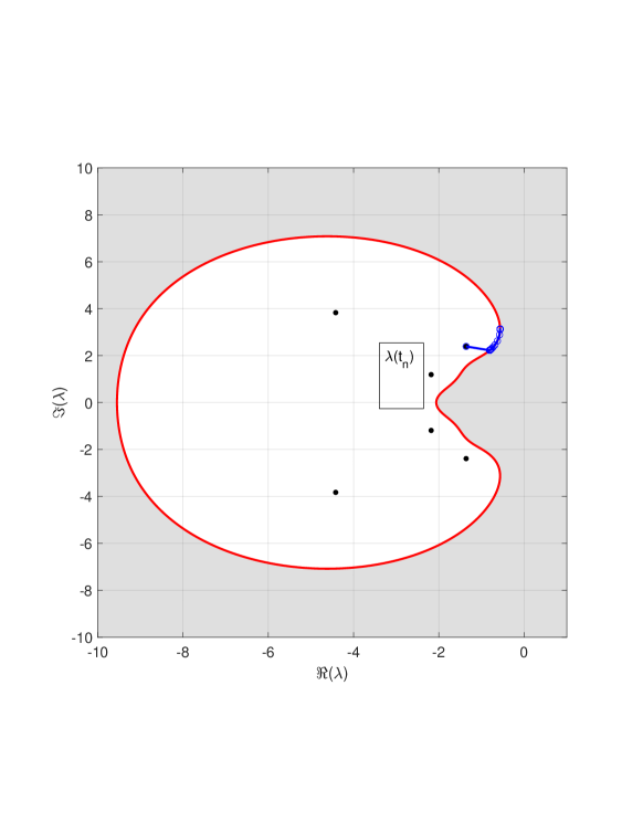
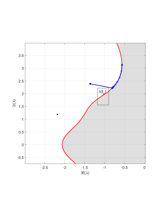
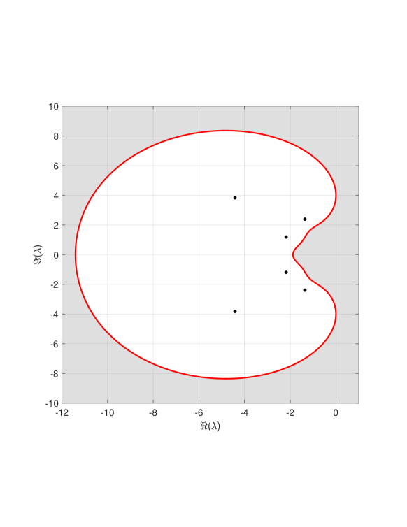
Fig. 1.1: Upper left picture: spectral value set of Example (1.53) and trajectory of the splitting method ($\varepsilon=0.1$). Upper right picture: zoom of the spectral value set and of the trajectory of the splitting method close to the rightmost point. Lower picture: Spectral value set for the value $\varepsilon=\varepsilon_{4}$ in Table 1.1. The picture illustrates that the set is tangential to the imaginary axis.

VII.2 $\mathcal{H}_{\infty}$-robustness of controllability

In this section we ask for the robustness of controllability of a given linear time-invariant system (0.1). We consider the operator nearness problem of finding the distance of a given controllable system to the nearest uncontrollable system, where the distance is taken as the $\mathcal{H}_{\infty}$-norm of the perturbation to the transfer function. This is a natural metric that measures the change in the input-output behaviour due to the perturbation of the system matrices. We propose and study a two-level algorithm that extends the algorithm of the preceding section.

VII.2.1 $\mathcal{H}_{\infty}$-nearest uncontrollable system

The linear time-invariant system (0.1) is controllable if and only if the $n\times(n+p)$ matrix

$$(A-\lambda I,B)\> \lambda\in\mathbb{C}$$ has full row rank for all . (2.1)

For this, it obviously suffices that the condition holds for the eigenvalues of $A$. Hence, a system is uncontrollable if and only if there exists an eigenvalue $\lambda_{A}$ of $A$ with corresponding left eigenvector $x_{A}$ such that

$$x_{A}^{*}B=0.$$

We consider the problem of finding the distance of a given controllable system (0.1) to the set of uncontrollable systems with the same matrices $A$, $C$ and $D$, but with perturbed input–state matrix $\widetilde{B}=B+\Delta B.$

Here an important question arises: which distance? We might minimize the Frobenius norm of $\Delta B$ under the condition that the perturbed system becomes uncontrollable (which would yield $\Delta B=-x_{A}x_{A}^{*}B$ for a left eigenvector $x_{A}$ to one of the eigenvalues of $A$), but this choice of a distance is not invariant under similarity transformations of $A$,

$$A\to V^{-1}AV,\quad B\to V^{-1}B,\quad C\to CV,$$ (2.2)

which leave the matrix transfer function $H(\lambda)=C(\lambda I-A)^{-1}B+D$ invariant and hence also the input-output map $y=H(\partial_{t})u$. We therefore measure the distance by the $L^{2}$ operator norm of the difference of the perturbed and unperturbed input-output operators, $\Delta H(\partial_{t})=\widetilde{H}(\partial_{t})-H(\partial_{t})$. This $L^{2}$ operator norm is the $\mathcal{H}_{\infty}$-norm of the perturbation $\Delta H(\lambda)=C(\lambda I-A)^{-1}\Delta B$ to the matrix transfer function. Considering real system matrices $(A,B,C,D)$ and real perturbations $\Delta B$, we arrive at the following operator nearness problem.

Problem. Given a controllable system (0.1), find a perturbation $\Delta B\in\mathbb{R}^{n,p}$ such that the perturbed input–state matrix $B+\Delta B$ yields an uncontrollable system and such that the perturbation to the transfer function, $\Delta H(\lambda)=C(\lambda I-A)^{-1}\Delta B\/$ for ${\mbox{\rm Re}}\,\lambda\geq 0$, is of minimal $\mathcal{H}_{\infty}$-norm.

Let $\lambda_{A}$ be an eigenvalue of $A$ with normalized left eigenvector $x_{A}$. We consider perturbations $R$ to $B$ that satisfy the uncontrollability condition $x_{A}^{*}(B+R)=0$, i.e.,

$$x_{A}^{*}R=-x_{A}^{*}B.$$ (2.3)

In the following we choose some left eigenvector $x_{A}$ of $A$ and denote the corresponding admissible affine space by

$$\mathcal{R}=\{R\in\mathbb{R}^{n,p}\,:\,R\text{ satisfies \eqref{R-cond} }\}.$$

Our proposed algorithm is based on the following characterization.

• ($\mathcal{H}_{\infty}$-distance to uncontrollability).  With the spectral value set abscissa as in (1.11),

  $$\alpha_{\varepsilon}(A,R,C,0)=\max_{\|E\|_{F}=1}{\mbox{\rm Re}}\,\lambda(A+\varepsilon REC),$$

  where $\lambda(M)$ is a rightmost eigenvalue of $M$, let

  $$R(\varepsilon)=\arg\min_{R\in\mathcal{R}}\alpha_{\varepsilon}(A,R,C,0)\quad\text{ and }$$

  $$\varepsilon_{\star}=\inf\{\varepsilon>0\,:\,\alpha_{\varepsilon}(A,R(\varepsilon),C,0)=0\}.$$ (2.4)

  Then, $\Delta B=R(\varepsilon_{\star})$ is a perturbation to the input–state matrix $B$ such that the perturbed system $(A,B+\Delta B,C,D)$ is not controllable and has minimal $\mathcal{H}_{\infty}$-distance between the transfer functions of the unperturbed system and uncontrollable perturbed systems with $\Delta B\in\mathcal{R}\,$. This $\mathcal{H}_{\infty}$-distance equals $1/\varepsilon_{\star}$.

  • For $R\in\mathcal{R}$, we denote the difference of the transfer functions corresponding to the systems $(A,B+R,C,D)$ and $(A,B,C,D)$ by

    $$\Delta H_{R}(\lambda)=C(\lambda I-A)^{-1}R.$$

    By Theorem VII.1.3, we have

    $$\|\Delta H_{R}\|_{\infty}=\frac{1}{\varepsilon_{R}}\quad\text{with}\quad\varepsilon_{R}=\min\{\varepsilon>0\,:\,\alpha_{\varepsilon}(A,R,C,0)=0\}$$

    and therefore

    $$\min_{R\in\mathcal{R}}\|\Delta H_{R}\|_{\infty}=\frac{1}{\varepsilon_{\max}}\quad\text{with}\quad\varepsilon_{\max}=\max_{R\in\mathcal{R}}\varepsilon_{R}.$$

    We now prove that $\varepsilon_{\max}$ equals $\varepsilon_{\star}$ of (2.4). Since the spectral value set abscissa depends monotonically on $\varepsilon$ and we have $\alpha_{\varepsilon_{\star}}(A,R,C,0)\geq 0$ for all $R\in\mathcal{R}$ and $\alpha_{\varepsilon_{\star}}(A,R,C,0)=0$ for some $R\in\mathcal{R}$, we obtain $\varepsilon_{\star}\geq\varepsilon_{R}$ for all $R\in\mathcal{R}$ and $\varepsilon_{\star}=\varepsilon_{R}$ for some $R\in\mathcal{R}$, and hence $\varepsilon_{\star}=\varepsilon_{\max}$. This yields the stated result.   $\sqcap$$\sqcup$

VII.2.2 Multi-level iteration

Theorem VII.2.1 motivates us to consider the following schematic multi-level iteration, for which we will provide details in the following subsections.

• Innermost iteration: For a given $\varepsilon>0$ and $R\in\mathcal{R}$, compute the spectral value set abscissa $\alpha_{\varepsilon}(A,R,C,0)$, e.g., by the rank-1 gradient flow algorithm of the preceding section. This algorithm also yields a rank-1 matrix $E_{\varepsilon}(R)\in\mathbb{C}^{n,n}$ of Frobenius norm 1 such that

  $$\alpha_{\varepsilon}(A,R,C,0)=\max_{E\in\mathbb{C}^{n,n},\,\|E\|_{F}=1}{\mbox{\rm Re}}\,\lambda(A+\varepsilon REC)={\mbox{\rm Re}}\,\lambda(A+\varepsilon RE_{\varepsilon}(R)C),$$ (2.5)

  where $\lambda(M)$ is a rightmost eigenvalue of a matrix $M$.

• Inner iteration: For a given $\varepsilon>0$, compute

  $$R(\varepsilon)=\arg\min_{R\in\mathcal{R}}\alpha_{\varepsilon}(A,R,C,0),$$ (2.6)

  e.g. by a gradient flow as described below.

• Outer iteration: Compute the zero $\varepsilon_{\star}$ of the monotonically growing function

  $$\phi(\varepsilon)=\alpha_{\varepsilon}(A,R(\varepsilon),C,0).$$ (2.7)

  We use a combined Newton–bisection method for this scalar equation, similar to the preceding section.

The zero $\varepsilon_{\star}$ depends on the chosen left eigenvector $x_{A}$ of $A$, which appears in (2.3) and hence in the definition of $\mathcal{R}\,$. While in theory we would have to compute $\varepsilon_{\star}=\varepsilon_{\star}(x_{A})$ for each eigenvector $x_{A}$ and then choose the maximal value among the $\varepsilon_{\star}(x_{A})$, we can expect that in practice it suffices to choose just a few eigenvectors $x_{A}$ for which $x_{A}^{*}B$ has smallest norms. (Note that $x_{A}^{*}B=(x_{A}^{*}V)(V^{-1}B)$ is invariant under transformations (2.2).)

For the maximal $\varepsilon_{\star}$ we have that $\Delta B=R(\varepsilon_{\star})$ is a perturbation to the input–state matrix $B$ such that the perturbed system $(A,B+\Delta B,C,D)$ is not controllable and has the minimal $\mathcal{H}_{\infty}$-distance $1/\varepsilon_{\star}$ between the transfer functions of the unperturbed and perturbed systems.

VII.2.3 Inner iteration: constrained gradient flow

We start with the free gradient of the functional in the inner iteration.

• (Derivative of the spectral value set abscissa).  Let $R(t)\in\mathbb{R}^{n,p}$, for real $t$ near $t_{0}$, be a continuously differentiable path of matrices, with the derivative denoted by $\dot{R}(t)$. Let $E(t)=E_{\varepsilon}(R(t))\in\mathbb{C}^{n,n}$ of Frobenius norm 1 be such that

  $$\alpha_{\varepsilon}(A,R(t),C,0)={\mbox{\rm Re}}\,\lambda(A+\varepsilon R(t)E(t)C)$$

  and the rightmost eigenvalue on the right-hand side is simple, with left and right eigenvectors $x(t)$ and $y(t)$, of norm 1 and with positive inner product. Let $\kappa(t)=1/(x(t)^{*}y(t))$. Assume that $x(t)^{*}R(t)\neq 0$ and $Cy(t)\neq 0$. Then we have, omitting the argument $t$ on the right-hand side,

  $$\frac{1}{\varepsilon\kappa(t)}\,\frac{d}{dt}\,\alpha_{\varepsilon}(A,R(t),C,0)=\langle G_{R},\dot{R}\rangle\quad\text{ with }\quad G_{R}={\mbox{\rm Re}}\bigl{(}x(ECy)^{*}\bigr{)}.$$

  • We have

    $$\frac{1}{\varepsilon\kappa(t)}\,\frac{d}{dt}\,{\mbox{\rm Re}}\,\lambda(A+\varepsilon R(t)E(t)C) ={\mbox{\rm Re}}\,x^{*}(\dot{R}EC+R\dot{E}C)y$$

    $$=\langle{\mbox{\rm Re}}\,x(ECy)^{*},\dot{R}\rangle+{\mbox{\rm Re}}\,\langle(R^{T}x)(Cy)^{*},\dot{E}\rangle$$

    $$=\langle G_{R},\dot{R}\rangle+{\mbox{\rm Re}}\,\langle G_{E},\dot{E}\rangle$$

    with $G_{R}={\mbox{\rm Re}}\bigl{(}x(ECy)^{*}\bigr{)}$ and $G_{E}=(R^{T}x)(Cy)^{*}$. We show that the last term vanishes. Since $E(t)$ is a stationary point of the functional $F_{\varepsilon}(E)={\mbox{\rm Re}}\,\lambda(A+\varepsilon REC)$ (with $R=R(t)$ for a fixed $t$) under the constraint of Frobenius norm 1, and since $G_{E}$ is nonzero by assumption, we find once again, as in Chapter II, that $E=\mu G_{E}$ for some nonzero real factor $\mu$. We then note, omitting the argument $t$ on the right-hand side,

    $$0=\frac{1}{2}\,\frac{d}{dt}\,\|E(t)\|^{2}={\mbox{\rm Re}}\langle E,\dot{E}\rangle=\mu\,{\mbox{\rm Re}}\langle G_{E},\dot{E}\rangle.$$

    This yields the stated result.   $\sqcap$$\sqcup$

Constrained gradient flow.

Choosing $\dot{R}$ such that it points in the direction of steepest admissible descent under the linear constraint (2.3), we arrive at the projected gradient system in which we take the constraint $x_{A}^{*}\dot{R}=0$ into account:

$$\dot{R}=-(I-P_{x_{A}})\,G_{R}\quad\text{ with }\quad G_{R}={\mbox{\rm Re}}\bigl{(}x(ECy)^{*}\bigr{)},$$ (2.8)

where $P_{x_{A}}$ is the orthogonal projection onto the range of $({\mbox{\rm Re}}\,x_{A},{\mbox{\rm Im}}\,x_{A})$ and $E=E_{\varepsilon}(R)$ is the perturbation that yields the spectral value set abscissa (computed in the innermost iteration as in Section VII.1).

VII.2.4 Outer iteration

For the outer iteration we again use a Newton method, which is justified under additional conditions, and we fall back to bisection when the Newton iteration does not work satisfactorily; cf. Section IV.1.5. Under the following assumption, the real function $\phi$ of (2.7) is differentiable and we will give a simple formula for its derivative.

• For $\varepsilon$ in a neighbourhood of $\varepsilon_{\star}$, we assume the following for the optimizer $R(\varepsilon)$ of the inner iteration and $E(\varepsilon)=E_{\varepsilon}(R(\varepsilon))$ of the innermost iteration:

  • The eigenvalue $\lambda(\varepsilon)=\lambda(A+\varepsilon R(\varepsilon)E(\varepsilon)C)$ is a simple eigenvalue, with normalized left and right eigenvectors denoted by $x(\varepsilon)$ and $y(\varepsilon)$.

  • The map $\varepsilon\mapsto(E(\varepsilon),R(\varepsilon))$ is continuously differentiable.

  • The partial gradient $G_{E}(\varepsilon)=(R(\varepsilon)^{T}x(\varepsilon))(Cy(\varepsilon))^{*}$ is nonzero.

  Theorem IV.IV.1.4 extends to the present situation. We again denote the eigenvalue condition number by $\kappa(\varepsilon)=1/(x(\varepsilon)^{*}y(\varepsilon))>0.$
  

  • (Derivative for the Newton iteration).  Under Assumption VII.2.4, the function $\phi(\varepsilon)=\alpha_{\varepsilon}(A,R(\varepsilon),C,0)$ is continuously differentiable in a neighbourhood of $\varepsilon_{\star}$ and its derivative is given as

    $$\phi^{\prime}(\varepsilon)=\kappa(\varepsilon)\,\|G_{E}(\varepsilon)\|_{F}>0.$$ (2.9)

    • By Lemma VII.2.3 we obtain, with $G_{R}(\varepsilon)=x(\varepsilon)(E(\varepsilon)Cy(\varepsilon))^{*}$ and indicating by ^′ differentiation w.r.t. $\varepsilon$,

      $$\frac{1}{\kappa(\varepsilon)}\,\frac{d}{d\varepsilon}\alpha_{\varepsilon}(A,R(\varepsilon),C,0)$$

      $$=\frac{1}{\kappa(\varepsilon)}\,\frac{d}{d\varepsilon}\alpha_{\varepsilon}(A,R(\eta),C,0)\Big{|}_{\eta=\varepsilon}+\frac{1}{\kappa(\varepsilon)}\,\frac{d}{d\varepsilon}\alpha_{\eta}(A,R(\varepsilon),C,0)\Big{|}_{\eta=\varepsilon}$$

      $$={\mbox{\rm Re}}\,\langle G_{E}(\varepsilon),E(\varepsilon)\rangle+{\mbox{\rm Re}}\,\langle G_{R}(\varepsilon),R^{\prime}(\varepsilon)\rangle.$$

      As in the proof of Theorem IV.IV.1.4 we find

      $${\mbox{\rm Re}}\bigl{\langle}G_{E}(\varepsilon),E(\varepsilon)\bigr{\rangle}=\|G_{E}(\varepsilon)\|_{F}.$$

      In the stationary point $R(\varepsilon)$ of (2.8) we have $(I-P_{x_{A}})G_{R}(\varepsilon)=0$, that is, $G_{R}(\varepsilon)=P_{x_{A}}G_{R}(\varepsilon)$. On the other hand, because of (2.3) we have $P_{x_{A}}R^{\prime}(\varepsilon)=0$. Hence,

      $$\bigl{\langle}G_{R}(\varepsilon),R^{\prime}(\varepsilon))\bigr{\rangle}=\bigl{\langle}P_{x_{A}}G_{R}(\varepsilon),R^{\prime}(\varepsilon))\bigr{\rangle}=\bigl{\langle}G_{R}(\varepsilon),P_{x_{A}}R^{\prime}(\varepsilon))\bigr{\rangle}=0,$$

      which yields the result.   $\sqcap$$\sqcup$

VII.3 Nearest passive system

Consider the linear time-invariant system (0.1), which we here assume quadratic ($p=m$). The system is called passive if every input $u\in L^{2}(\mathbb{R}_{+},\mathbb{R}^{m})$ and its corresponding output $y$ satisfy the relation

$$\int_{0}^{T}y(t)^{\top}u(t)\,dt\geq 0\quad\ \text{ for all }\>T>0.$$ (3.1)

Passivity is a fundamental property in control theory. When a given system is not passive, it is often required to enforce passivity by modifying it such that it becomes passive, yet remains ‘near’ the given system. One approach, as discussed by Grivet-Talocia & Gustavsen (?) and to be adopted here, is to perturb only the state–output matrix $C\in\mathbb{R}^{m,n}$ to $C+\Delta C$ and to minimize a suitable norm of the perturbation such that the perturbed system is passive.

A favoured choice in the literature is to minimize the Frobenius norm of $\Delta C\,L$, where $L\in\mathbb{R}^{n,n}$ is a Cholesky factor of the controllability Gramian $G_{c}=LL^{T}$, which is the unique solution of the Lyapunov equation $AG_{c}+G_{c}A^{\top}=BB^{\top}$. This Gramian is symmetric positive definite for a controllable system, as will be assumed in the following. The squared norm $\langle\Delta C\,G_{c},\Delta C\rangle=\|\Delta C\,L\|_{F}^{2}$ is invariant under transformations (2.2) of the system matrices, as is readily checked. Based on the characterization of passivity via Hamiltonian matrices, we present a two-level algorithm for this minimization problem in the Frobenius norm.

In a different direction that appears not to have been addressed in the literature before, we present in Subsection VII.3.5 an algorithm for the problem of enforcing passivity by perturbing $C$ in such a way that the $\mathcal{H}_{\infty}$-norm of the difference between the transfer functions of the passive perturbed system and of the original system is minimized, similar to the approach in Section VII.2.

VII.3.1 Hamiltonian matrix related to passivity

By the Plancherel formula and the relation (1.2) of the matrix transfer function $H(\lambda)$, we have (with $u$ extended by 0 outside [0,T])

$$\int_{0}^{T}y(t)^{\top}u(t)\,dt ={\mbox{\rm Re}}\int_{\mathbb{R}}\mathcal{L}y(\mathrm{i}\omega)^{*}\mathcal{L}u(\mathrm{i}\omega)\,d\omega={\mbox{\rm Re}}\int_{\mathbb{R}}\mathcal{L}\bigl{(}H(\mathrm{i}\omega)u(\mathrm{i}\omega)\bigr{)})^{*}\mathcal{L}u(\mathrm{i}\omega)\,d\omega$$

$$=\frac{1}{2}\int_{\mathbb{R}}u(\mathrm{i}\omega)^{*}\bigl{(}H(\mathrm{i}\omega)+H(\mathrm{i}\omega)^{*}\bigr{)}u(\mathrm{i}\omega)\,d\omega,$$

and so we find that passivity (3.1) is equivalent to the property of positive realness of the transfer function:

$$H(\mathrm{i}\omega)+H(\mathrm{i}\omega)^{*}\text{ is positive semi-definite for all $\omega\in\mathbb{R}$}.$$ (3.2)

Since $H(\mathrm{i}\omega)\to D$ as $\omega\to\infty$, a necessary condition for (3.2) is that $D+D^{\top}$ is positive semi-definite.

Strict positive realness is defined in the same way, with ‘positive definite’ instead of ‘positive semi-definite’ for all $\omega\in\mathbb{R}\cup\{\infty\}$. A necessary condition is now that $D+D^{\top}$ is positive definite.

The following remarkable result can be found in Chapter 9 of the book by Grivet-Talocia & Gustavsen (?). It goes back to Boyd, Balakrishnan & Kabamba (?) and in its conceptual origins further back to Byers (?). It characterizes strict positive realness, which is a condition on the transfer function on the whole imaginary axis, by the location of the eigenvalues of a single Hamiltonian matrix built from the system matrices.

• (Passivity and eigenvalues of a Hamiltonian matrix).  The matrix transfer function $H(\cdot)$ is strictly positive real if and only if $D+D^{\top}$ is positive definite and the Hamiltonian matrix

  $$K=\begin{pmatrix}A&0\\ 0&-A^{T}\end{pmatrix}-\begin{pmatrix}B\\ -C^{\top}\end{pmatrix}(D+D^{\top})^{-1}\begin{pmatrix}C^{\top}\\ B\end{pmatrix}^{\top}\ \in\mathbb{R}^{2n\times 2n}$$ (3.3)

  has no eigenvalues on the imaginary axis.

  In the following we will consider the Hamiltonian matrix also for systems with perturbed state–output matrices $C+\Delta C$. To indicate the dependence on $C$, we write $K(C)$ for $K$ of (3.3).

VII.3.2 Two-level iteration

Theorem VII.3.1 leads us to the following matrix nearness problem, which is reminiscent of Problem B in Section VI.2. Here, the matrix $L\in\mathbb{R}^{n,n}$ is usually chosen as a Cholesky factor of the controllability Gramian, as mentioned above.

Problem (F). Given a system (0.1) with positive definite matrix $D+D^{\top}$ for which the Hamiltonian matrix $K(C)$ has some purely imaginary eigenvalues, and given $\delta>0$, compute a perturbed state–output matrix $C+\Delta C$ with minimal $\|\Delta C\,L\|_{F}$ such that all eigenvalues of $K(C+\Delta C)$ have a real part of absolute value at least $\delta$.

The proposed algorithm is a two-level iterative method similar to the second method of Section VI.2.5.

• Inner iteration: For a given $\varepsilon>0$, we use a (low-rank) gradient system to solve the eigenvalue optimization problem, over $E\in\mathbb{R}^{p\times n}$ with $\|E\|_{F}=1$,

  $$E(\varepsilon)=\arg\max_{\|E\|_{F}=1}\ {\mbox{\rm Re}}\,\lambda\bigl{(}K(C+\varepsilon EL^{-1})\bigr{)},$$ (3.4)

  where $\lambda(K)$ is an eigenvalue of minimal nonnegative real part (chosen with the largest nonnegative imaginary part) of a real Hamiltonian matrix $K$.

• Outer iteration: We compute the smallest $\varepsilon$ such that

  $$\phi(\varepsilon):={\mbox{\rm Re}}\,\lambda\bigl{(}K(C+\varepsilon E(\varepsilon)L^{-1})\bigr{)}=\delta$$ (3.5)

  for the given small threshold $\delta>0$. This uses a mixed Newton–bisection method and, for very small $\delta$, the asymptotic square-root behavior $\phi(\varepsilon)\sim\sqrt{\varepsilon-\varepsilon_{\star}}$ as the eigenvalue tends to the imaginary axis at perturbation size $\varepsilon_{\star}$; see Theorem VI.VI.2.3.

VII.3.3 Norm- and rank-constrained gradient flows

In this subsection we show how to deal with the inner iteration, once again following and adapting the by now well-trodden path of Chapter II, here in the real version of Section V.1.

In the resulting algorithm we do not move eigenvalues of Hamiltonian matrices on the imaginary axis. Instead, like in the second algorithm of Section VI.2.5, we work with Hamiltonian matrices all whose eigenvalues are off the imaginary axis, corresponding to perturbed matrices $C$ that yield a passive system. We move eigenvalues with smallest positive real part toward the imaginary axis, starting from a non-optimal passive perturbation of the original, non-passive system. This starting perturbation can come from a computationally inexpensive but non-optimal passivity enforcement algorithm.

Free gradient. The following lemma will allow us to compute the steepest descent direction of the functional $F_{\varepsilon}(E)=-{\mbox{\rm Re}}\,\lambda\bigl{(}K(C+\varepsilon EL^{-1})\bigr{)}$.

• (Real gradient).  Let $E(t)\in\mathbb{R}^{m,n}$, for real $t$ near $t_{0}$, be a continuously differentiable path of matrices, with the derivative denoted by $\dot{E}(t)$. Assume that $\lambda(t)$ is a simple eigenvalue of $K(C+\varepsilon E(t)L^{-1})\bigr{)}$ depending continuously on $t$, with associated eigenvectors $x(t)$ and $y(t)$ normalized by (1.23), and let $\kappa(t)=1/(x(t)^{*}y(t))>0.$
  Then, the derivative of $F_{\varepsilon}(E(t))={\mbox{\rm Re}}\,\lambda\bigl{(}K(C+\varepsilon E(t)L^{-1})\bigr{)}$ is given by

  $$\frac{1}{\varepsilon\kappa(t)}\,\frac{d}{dt}F_{\varepsilon}(E(t))=\,\bigl{\langle}G_{\varepsilon}(E(t)),\dot{E}(t)\bigr{\rangle}$$ (3.6)

  with the (rescaled) real gradient

  $$G_{\varepsilon}(E)=K^{\prime}(C+\varepsilon EL^{-1})^{\ast}[{\mbox{\rm Re}}(xy^{*})]L^{-\top}\in\mathbb{R}^{m,n},$$ (3.7)

  where $K^{\prime}(C)^{\ast}:\mathbb{R}^{2n,2n}\to\mathbb{R}^{m,n}$ is the adjoint of the derivative $K^{\prime}(C):\mathbb{R}^{m,n}\to\mathbb{R}^{2n,2n}$ defined by $\langle K^{\prime}(C)^{\ast}[W],Z\rangle=\langle W,K^{\prime}(C)[Z]\rangle$ for all $W\in\mathbb{R}^{2n,2n}$ and $Z\in\mathbb{R}^{m,n}$.

  • By the derivative formula for simple eigenvalues and the chain rule, we have (omitting the ubiquitous argument $t$ after the first equality sign)

    $$\frac{d}{dt}\,{\mbox{\rm Re}}\,\lambda\bigl{(}K(C+\varepsilon E(t)L^{-1})\bigr{)}=\kappa\,{\mbox{\rm Re}}\Bigl{(}x^{*}K^{\prime}(C+\varepsilon EL^{-1})[\varepsilon\dot{E}L^{-1}]y\Bigr{)}$$

    $$=\kappa\bigl{\langle}{\mbox{\rm Re}}(xy^{*}),K^{\prime}(C+\varepsilon EL^{-1})[\varepsilon\dot{E}L^{-1}]\bigr{\rangle}=\kappa\varepsilon\bigl{\langle}K^{\prime}(C+\varepsilon EL^{-1})^{\ast}[{\mbox{\rm Re}}(xy^{*})]L^{-\top},\dot{E}\bigr{\rangle},$$

    which yields the stated result.   $\sqcap$$\sqcup$

  An explicit formula for the adjoint of the derivative of $K$ is given next.

  • (Adjoint of the derivative).  For $W=\begin{pmatrix}W_{11}&W_{12}\\ W_{21}&W_{22}\end{pmatrix}\in\mathbb{R}^{2n\times 2n}$ partitioned according to the $n\times n$ blocks of $K(C)$, we have (with $T=D+D^{\top}$ for short)

    $$K^{\prime}(C)^{\ast}[W]=-T^{-1}B^{\top}(W_{11}-W_{22}^{\top})+T^{-1}C\,(W_{21}+W_{21}^{\top}).$$ (3.8)

    • A noteworthy consequence of (3.8) is that $G_{\varepsilon}(E)$ of (3.7) has rank at most 8. (The rank is at most 4 for real eigenvalues.)

    • For any path $C(t)$ we have $\dot{K}(t)=\frac{d}{dt}K(C(t))=K^{\prime}(C(t))[\dot{C}(t)]$ and hence

      $$\langle K^{\prime}(C)^{\ast}[W],\dot{C}\rangle=\langle W,K^{\prime}(C)[\dot{C}]\rangle=\langle W,\dot{K}\rangle.$$

      Differentiation of (3.3) yields

      $$\dot{K}= \ -\begin{pmatrix}0\\ -\dot{C}^{\top}\end{pmatrix}T^{-1}\begin{pmatrix}C^{\top}\\ B\end{pmatrix}^{\top}-\begin{pmatrix}B\\ -C^{\top}\end{pmatrix}T^{-1}\begin{pmatrix}\dot{C}^{\top}\\ 0\end{pmatrix}^{\top}.$$

      We note that

      $$\left\langle W,\begin{pmatrix}0\\ -\dot{C}^{\top}\end{pmatrix}T^{-1}\begin{pmatrix}C^{\top}\\ B\end{pmatrix}^{\top}\right\rangle=\left\langle W\begin{pmatrix}C^{\top}\\ B\end{pmatrix}T^{-1},\begin{pmatrix}0\\ -\dot{C}^{\top}\end{pmatrix}\right\rangle$$

      $$\quad=-\bigl{\langle}(W_{21}C^{\top}+W_{22}B)T^{-1},\dot{C}^{\top}\bigr{\rangle}=-\bigl{\langle}((W_{21}C^{\top}+W_{22}B)T^{-1})^{\top},\dot{C}\bigr{\rangle}$$

      $$\left\langle W,\begin{pmatrix}B\\ -C^{\top}\end{pmatrix}T^{-1}\begin{pmatrix}\dot{C}^{\top}\\ 0\end{pmatrix}^{\top}\right\rangle=\langle T^{-1}(B^{\top},-C)W,(\dot{C},0)\rangle$$

      $$\quad=\bigl{\langle}T^{-1}(B^{\top}W_{11}-CW_{21}),\dot{C}\bigr{\rangle}$$

      so that finally

      $$\langle K^{\prime}(C)^{\ast}[W],\dot{C}\rangle=\langle W,\dot{K}\rangle=\langle-T^{-1}B^{\top}(W_{11}-W_{22}^{\top})+T^{-1}C\,2\,\mathrm{Sym}(W_{21}),\dot{C}\rangle$$

      for all $\dot{C}\in\mathbb{R}^{m,n}$. This yields $K^{\prime}(C)^{\ast}[W]$ as stated.   $\sqcap$$\sqcup$

  Norm-constrained gradient flow. As in Section V.1, we consider the projected gradient flow on the manifold of $m\times n$ real matrices of unit Frobenius norm:

  $$\dot{E}=-G_{\varepsilon}(E)+\left\langle G_{\varepsilon}(E),E\right\rangle E,$$ (3.9)

  where $G_{\varepsilon}(E)$ is defined by (3.7) via an eigentriple $(\lambda$, $x$, $y)$ of the Hamiltonian matrix $K(C+\varepsilon EL^{-1})$ with $\lambda$ the target eigenvalue of minimal nonnegative real part (and among these, the one with largest nonnegative imaginary part). The Frobenius norm 1 is conserved along trajectories.

  We now follow closely the programme of Section V.1: We again have the monotonic decay of $F_{\varepsilon}(E(t))$ as in (II.1.7), and the characterization of stationary points as given in Theorem II.II.2.3 also extends: Let $E\in\mathbb{C}^{m,n}$ with $\|E\|_{F}=1$ be such that the target eigenvalue $\lambda$ of $K(C+\varepsilon EL^{-1})$ is simple and $G_{\varepsilon}(E)\neq 0$. Then, $E$ is a stationary point of the differential equation (3.9) if and only if $E$ is a real multiple of $G_{\varepsilon}(E)$. Together with Remark VII.3.3, this implies the following.

• (Rank of optimizers).  If $E$ is an optimizer of the eigenvalue optimization problem (3.4) and if $G_{\varepsilon}(E)\neq 0$, then $E$ is of rank at most $8$.

  As in Section V.1, this motivates us to constrain the differential equation (3.9) to a manifold of real low-rank matrices, which turns out to be computationally favourable for large systems.

  Rank-8 constrained gradient flow. In the same way as in Section V.1.4, this time with rank $r=8$, we orthogonally project the right-hand side of (3.9) onto the tangent space at $E$ of the manifold $\mathcal{M}_{r}\subset\mathbb{R}^{m,n}$ of real rank-$r$ matrices, so that solutions starting with rank $r$ retain the rank $r$:

  $$\dot{E}=P_{E}\Bigl{(}-G_{\varepsilon}(E)+\langle G_{\varepsilon}(E),E\rangle E\Bigr{)}.$$ (3.10)

  Then also the Frobenius norm 1 is conserved (see (II.1.15)), and $F_{\varepsilon}(E(t))$ decays monotonically (see (II.1.17)).

  Using the SVD-like factorization $E=USV^{\top}$, where $U\in\mathbb{R}^{m,r}$ and $V\in\mathbb{R}^{n,r}$ have orthonormal columns and $S\in\mathbb{R}^{r,r}$, the seemingly abstract differential equation (3.10) is solved numerically for the factors $U,V,S$ as described in Section V.1.5.

  Using the low-rank structure in the eigenvalue computation. For the computation of the gradient matrix $G_{\varepsilon}(E)$, one needs to compute the eigenvalue of smallest positive real part and the associated left and right eigenvectors of the Hamiltonian matrix $K(C+\varepsilon EL^{-1})$. Except in the very first step of the algorithm, one can make use of the eigenvalue of smallest real part of the previous step in an inverse iteration (and possibly of the eigenvalues of second and third smallest real part etc. to account for a possible exchange of the leading eigenvalue).

  Moreover, we get from a perturbation $\varepsilon EL^{-1}$ with $E=U\Sigma V^{\top}$ of rank 8 that $C$ is perturbed by $\Delta C=\varepsilon EL^{-1}=\varepsilon(U\Sigma)(L^{-\top}V)^{\top}$ of the same rank 8, which yields the perturbed Hamiltonian matrix

  $$K(C+\Delta C)=K(C)+\Delta K,$$

  where the perturbation $\Delta K$ is still of moderate rank in view of (3.3). This fact can be used in the computation of the required eigenvalues in the case of a high-dimensional system, using the Sherman–Morrison–Woodbury formula in an inverse iteration.

  If $p\ll n$, then $K(C)$ can be viewed as a low-rank perturbation to the matrix

  $$\begin{pmatrix}A&0\\ 0&-A^{\top}\end{pmatrix}.$$

  With the Sherman–Morrison–Woodbury formula, this can yield an efficient inverse iteration when $A$ is a large and sparse matrix for which shifted linear systems can be solved efficiently.

VII.3.4 Outer iteration

For the solution of the scalar nonlinear equation (3.5) we use a mixed Newton–bisection method as in Section IV.1.5 or, for small $\delta$, the square root model and bisection as in Section VI.2.4.

Numerical results obtained with the above method for passivity enforcement are given by Fazzi, Guglielmi & Lubich (?).

VII.3.5 $\mathcal{H}_{\infty}$-nearest passive system

We extend the approach of Section VII.2 to the problem of $\mathcal{H}_{\infty}$-optimal passivity enforcement.

Problem ($\mathcal{H}_{\infty}$). Given a system (0.1) with positive definite matrix $D+D^{\top}$ for which the Hamiltonian matrix $K(C)$ has some purely imaginary eigenvalues, and given $\delta>0$, compute a perturbed state–output matrix $C+\Delta C$ with minimal $\mathcal{H}_{\infty}$-norm of the perturbation to the transfer function, $\Delta H(\lambda)=\Delta C(\lambda I-A)^{-1}B$, such that all eigenvalues of $K(C+\Delta C)$ have a real part of absolute value at least $\delta$.

We propose a multi-level approach similar to Section VII.2. We use the variable $S$ for $\Delta C$.

• Innermost iteration: For given $\varepsilon>0$ and $S\in\mathbb{R}^{m,n}$, compute the spectral value set abscissa $\alpha_{\varepsilon}(A,B,S,0)$, e.g., by the rank-1 gradient flow algorithm of the Section VII.1. This algorithm also yields a rank-1 matrix $E_{\varepsilon}(S)\in\mathbb{C}^{n,n}$ of Frobenius norm 1 such that

  $$\alpha_{\varepsilon}(A,B,S,0)=\max_{E\in\mathbb{C}^{n,n},\,\|E\|_{F}=1}{\mbox{\rm Re}}\,\lambda(A+\varepsilon BES)={\mbox{\rm Re}}\,\lambda(A+\varepsilon BE_{\varepsilon}(S)S),$$ (3.11)

  where $\lambda(M)$ is a rightmost eigenvalue of a matrix $M$.

• Inner iteration: For given $\delta>0$ and $\varepsilon>0$, we use a constrained gradient system to solve the constrained eigenvalue optimization problem, over $S\in\mathbb{R}^{m,n}$,

  $$S(\varepsilon)=\arg\min_{S}\alpha_{\varepsilon}(A,B,S,0),\quad\ \text{ subject to}\quad{\mbox{\rm Re}}\,\lambda_{H}(K(C+S))\geq\delta,$$ (3.12)

  where $\lambda_{H}(K)$ is an eigenvalue of minimal nonnegative real part of a Hamiltonian matrix $K\in\mathbb{R}^{2n,2n}$.

• Outer iteration: Compute the zero $\varepsilon_{\star}$ of the monotonically growing function

  $$\phi(\varepsilon)=\alpha_{\varepsilon}(A,B,S(\varepsilon),0).$$ (3.13)

  We use a combined Newton–bisection method for this scalar equation.

We then have the following analogue of Theorem VII.2.1, which is proved by the same argument based on Theorem VII.1.3.

• ($\mathcal{H}_{\infty}$-distance).  Let $\varepsilon_{\star}>0$ be the exact solution of the problem (3.11)–(3.13). Then, the perturbed state–output matrix $C+S(\varepsilon_{\star})$ yields a passive system having ${\mbox{\rm Re}}\,\lambda(K(C+S))\geq\delta$ with minimal $\mathcal{H}_{\infty}$-distance between the transfer functions of the perturbed and unperturbed systems. This $\mathcal{H}_{\infty}$-distance equals $1/\varepsilon_{\star}$.

For the inner iteration we use a constrained gradient flow, based on the following direct analogue of Lemma VII.2.3 and on Lemma VII.3.3.

• (Derivative of the spectral value set abscissa).  Let $S(t)\in\mathbb{R}^{m,n}$, for real $t$ near $t_{0}$, be a continuously differentiable path of matrices, with the derivative denoted by $\dot{S}(t)$. Let $E(t)=E_{\varepsilon}(S(t))\in\mathbb{C}^{n,n}$ of Frobenius norm 1 be such that

  $$\alpha_{\varepsilon}(A,C,S(t),0)={\mbox{\rm Re}}\,\lambda(A+\varepsilon BE(t)S(t))$$

  and the rightmost eigenvalue on the right-hand side is simple, with left and right eigenvectors $x(t)$ and $y(t)$, of norm 1 and with positive inner product. Let $\kappa(t)=1/(x(t)^{*}y(t))$. Assume that $S(t)y(t)\neq 0$ and $x(t)^{*}B\neq 0$. Then we have, omitting the argument $t$ on the right-hand side,

  $$\frac{1}{\varepsilon\kappa(t)}\,\frac{d}{dt}\,\alpha_{\varepsilon}(A,B,S(t),0)=\langle G_{S},\dot{S}\rangle\quad\text{ with }\quad G_{S}={\mbox{\rm Re}}\bigl{(}(x^{*}BE)^{*}y^{*}\bigr{)}.$$

VII.4 Structured contractivity radius

A linear time-invariant system (0.1) is called contractive if its transfer function $H$ is bounded in the $\mathcal{H}_{\infty}$-norm by

$$\|H\|_{\infty}\leq 1,$$

and it is called strictly contractive if the above inequality is strict. Contractive systems play an important role as subsystems in large networks, because their composition remains contractive and thus yields well-controlled input-output relations. A strictly contractive system may be susceptible to perturbations (or uncertainties) in the entries of its matrices $(A,B,C,D)$, and it is then of interest to know which size of perturbations still guarantees contractivity. Here, we consider perturbations only in the state matrix $A$ and allow for structured perturbations $\Delta\in\mathcal{S}$, where the structure space $\mathcal{S}\subset\mathbb{C}^{n,n}$ is a given complex- or real-linear subspace, e.g. real matrices with a prescribed sparsity pattern. We study the following problem in this section.

Let $(A,B,C,D)$ be the system matrices of a strictly contractive linear time-invariant system. In particular, this implies $\|D\|_{2}<1$. We consider structured perturbations $A\to A+\Delta$ with $\Delta\in\mathcal{S}$, which yield perturbed transfer functions

$$H_{\Delta}(\lambda)=C(\lambda I-A-\Delta)^{-1}B+D.$$

Problem. Find the largest possible perturbation size $\delta_{\star}>0$ such that

$$\|H_{\Delta}\|_{\infty}\leq 1\quad\ \text{\it for all $\,\Delta\in\mathcal{S}\,$ with $\,\|\Delta\|_{F}\leq\delta_{\star}$\,.}$$

The number $\delta_{\star}>0$ measures the robustness of contractivity of a system and is called the $\mathcal{S}$-structured contractivity radius. We present and discuss a two-level algorithm that is closely related to that of Section V.6 with $\varepsilon=1$, to which it reduces for the special case $B=C=I$ and $D=0$.

VII.4.1 Two-level iteration

We consider the matrix $M(\Theta)$ of (1.5) that corresponds to $A+\Delta$ instead of $A$. So we let

$$M(\Delta,\Theta)=A+\Delta+B\Theta(I-D\Theta)^{-1}C.$$

By Theorem VII.1.1, $\|H_{\Delta}\|_{\infty}=1$ if and only if there exists $\Theta\in\mathbb{C}^{p,m}$ with $\|\Theta\|_{2}=1$ such that $M(\Delta,\Theta)$ has an eigenvalue with nonnegative real part. Moreover, the optimizing matrix $\Theta$ is of rank 1, and hence its Frobenius and 2-norms are the same. We define the functional $F_{\delta}(E^{\mathcal{S}},E)$ (for $E^{\mathcal{S}}\in\mathcal{S}$ and $E\in\mathbb{C}^{p,m}$, both of unit Frobenius norm) by

$$F_{\delta}(E^{\mathcal{S}},E)=-{\mbox{\rm Re}}\,\lambda\bigl{(}M(\delta E^{\mathcal{S}},E)\bigr{)},$$ (4.1)

where $\lambda(M)$ is the eigenvalue of $M$ of largest real part (and among those, the one with largest imaginary part). With this functional we follow the two-level approach of Section IV.1:

• Inner iteration: For a given $\delta>0$, we aim to compute matrices $E^{\mathcal{S}}(\delta)\in\mathcal{S}$ and $E(\delta)\in\mathbb{C}^{p,m}$, both of unit Frobenius norm, that minimize $F_{\delta}$:

  $$(E^{\mathcal{S}}(\delta),E(\delta))=\arg\min\limits_{E^{\mathcal{S}}\in\mathcal{S},E\in\mathbb{C}^{p,m}\atop\|E^{\mathcal{S}}\|_{F}=\|E\|_{F}=1}F_{\delta}(E^{\mathcal{S}},E).$$ (4.2)

• Outer iteration: We compute the smallest positive value $\delta_{\star}$ with

  $$\phi(\delta_{\star})=0,$$ (4.3)

  where $\phi(\delta)=F_{\delta}(E^{\mathcal{S}}(\delta),E(\delta))=\alpha_{\varepsilon}(A+\delta E^{\mathcal{S}}(\delta),B,C,D)$ for $\varepsilon=1$.

Provided that these computations succeed, we have from Theorem VII.1.3 that $\Delta_{\star}=\delta_{\star}E^{\mathcal{S}}(\delta_{\star})\in\mathcal{S}$ is a perturbation matrix with $\|H_{\Delta_{\star}}\|_{\infty}=1$, and $\delta_{\star}$ is the $\mathcal{S}$-structured contractivity radius.

VII.4.2 Rank-1 matrix differential equations for the inner iteration

The following lemma is obtained as in the proof of Lemma VII.1.5.

• (Structured gradient).  Let $E^{\mathcal{S}}(t)\in\mathcal{S}$ and $E(t)\in\mathbb{C}^{p,m}$, for real $t$ near $t_{0}$, be continuously differentiable paths of matrices. Assume that $\lambda(t)$ is a simple eigenvalue of $M(\delta E^{\mathcal{S}}(t),E(t))$ depending continuously on $t$, with associated left and right eigenvectors $x(t)$ and $y(t)$ normalized by (1.23), and let $\kappa(t)=1/(x(t)^{*}y(t))>0$. Then, the derivative of $F_{\delta}(E^{\mathcal{S}}(t),E(t))$ is given by

  $$\frac{1}{\kappa(t)}\,\frac{d}{dt}F_{\delta}(E^{\mathcal{S}}(t),E(t)) =\ {\mbox{\rm Re}}\,\bigl{\langle}G_{\Delta}^{\mathcal{S}}(\delta E^{\mathcal{S}}(t),E(t)),\delta\dot{E}^{\mathcal{S}}(t)\bigr{\rangle}$$ (4.4)

  $$\quad+{\mbox{\rm Re}}\,\bigl{\langle}G_{\Theta}(\delta E^{\mathcal{S}}(t),E(t)),\dot{E}(t)\bigr{\rangle}$$

  with the (rescaled) gradient

  $$G_{\Delta}^{\mathcal{S}}(\Delta,\Theta) =\Pi^{\mathcal{S}}(xy^{*})\in\mathcal{S},$$ (4.5)

  $$G_{\Theta}(\Delta,\Theta) =rs^{*}\in\mathbb{C}^{p,m},$$

  where $r,s$ are obtained from $x,y$ via (1.24).

Norm- and structure-constrained gradient flow.

Similar to Section V.6, we consider the projected gradient flow, with $G_{\Delta}^{\mathcal{S}}=G_{\Delta}^{\mathcal{S}}(\delta E^{\mathcal{S}},E)$ and $G_{\Theta}=G_{\Theta}(\delta E^{\mathcal{S}},E)$ for short,

$$\delta\dot{E}^{\mathcal{S}} =-G_{\Delta}^{\mathcal{S}}+{\mbox{\rm Re}}\left\langle G_{\Delta}^{\mathcal{S}},E^{\mathcal{S}}\right\rangle E^{\mathcal{S}},$$ (4.6)

$$\dot{E} =-G_{\Theta}+{\mbox{\rm Re}}\left\langle G_{\Theta},E\right\rangle E.$$

The unit Frobenius norm of $E^{\mathcal{S}}$ and $E$ is conserved along trajectories and the functional $F_{\delta}(E^{\mathcal{S}}(t),E(t))$ decreases monotonically. At a non-degenerate stationary point $(E^{\mathcal{S}},E)$, where $G_{\Delta}^{\mathcal{S}}$ and $G_{\Theta}$ do not vanish, we find that $E^{\mathcal{S}}$ and $E$ are real multiples of $G_{\Delta}^{\mathcal{S}}$ and $G_{\Theta}$, respectively. Hence, $E^{\mathcal{S}}$ is the projection onto $\mathcal{S}$ of a rank-1 matrix, and $E$ is a rank-1 matrix.

Rank-1 matrix differential equations.

To make use of the rank-1 structure of optimizers, we proceed as in Section V.6 and combine the rank-1 approaches of Sections II.2 and V.2. We consider differential equations for rank-1 matrices $Y(t)$ and $E(t)$, where the former yields $E^{\mathcal{S}}(t)=\Pi^{\mathcal{S}}Y(t)$. These differential equations are obtained from (6.6) by replacing $G_{\Delta}^{\mathcal{S}}$ and $G_{\Theta}$ by their projections $P_{Y}$ and $P_{E}$ onto the tangent spaces of the manifold of rank-1 matrices at $Y$ and $E$, respectively:

$$\delta\,\dot{Y} =-P_{Y}G_{\Delta}^{\mathcal{S}}+{\mbox{\rm Re}}\,\langle P_{Y}G_{\Delta}^{\mathcal{S}},E^{\mathcal{S}}\rangle Y\quad\text{ with }\ E^{\mathcal{S}}=\Pi^{\mathcal{S}}Y,$$ (4.7)

$$\dot{E} =-P_{E}G_{\Theta}+{\mbox{\rm Re}}\,\langle G_{\Theta},E\rangle E.$$

These differential equations yield rank-1 matrices $Y(t)$ and $E(t)$ and preserve the unit Frobenius norm of $E^{\mathcal{S}}(t)$ and $E(t)$. As in Sections II.2 and V.2 it is shown that under a nondegeneracy condition, the stationary points $(Y,E)$ of (4.7) correspond bijectively to the stationary points $(E^{\mathcal{S}},E)$ of (4.6) via $E^{\mathcal{S}}=\Pi^{\mathcal{S}}Y$ and with the same $E$. The differential equations are integrated numerically into a stationary point $(E^{\mathcal{S}},E)$ as is done in Sections II.2 and V.2, working with the vectors that define the rank-1 matrices $Y$ and $E$.

VII.4.3 Outer iteration

For the solution of the scalar equation $\phi(\delta)=0$ we use a combined Newton–bisection method as in Section IV.1. The derivative of $\phi$ for the Newton iteration is obtained with the arguments of the proof of Theorem IV.IV.1.4 (under analogous assumptions), which yields

$$\phi^{\prime}(\delta)=-\kappa(\delta)\,\|G_{\Delta}^{\mathcal{S}}(\delta E^{\mathcal{S}}(\delta),E(\delta))\|_{F}=-\kappa(\delta)\,\|\Pi^{\mathcal{S}}(x(\delta)y(\delta)^{*})\|_{F},$$

where $x(\delta)$ and $y(\delta)$ are left and right normalized eigenvectors associated with the rightmost eigenvalue of $M(\delta E^{\mathcal{S}}(\delta),E(\delta))$, and $\kappa(\delta)=1/(x(\delta)^{*}y(\delta))>0$.

VII.5 Descriptor systems

We consider a descriptor system, which formally differs from the system (0.1) only in that the derivative of the state vector is multiplied with a singular matrix $E\in\mathbb{R}^{n,n}$: for $t\geq 0$,

$$E\dot{z}(t) =Az(t)+Bu(t)$$ (5.1)

$$y(t) =Cz(t).$$

We choose zero initial values and assume that the input function $u$ can be extended by zero to a sufficiently differentiable function on the whole real axis. Since $E$ is singular, the equation for the state vector $z$ is now a differential-algebraic equation instead of a pure differential equation. Descriptor systems arise naturally in systems with state constraints and in modelling and composing networks of such systems.

We assume that all finite eigenvalues of the matrix pencil $A-\lambda E$ have negative real part, i.e.,

$$A-\lambda E\, \lambda\in\mathbb{C} {\mbox{\rm Re}}\,\lambda\geq 0$$ is invertible for all with . (5.2)

In particular, the matrix $A$ is invertible.

The matrix transfer function of the descriptor system is

$$H(\lambda)=C(\lambda E-A)^{-1}B,\qquad{\mbox{\rm Re}}\,\lambda\geq 0.$$ (5.3)

• In the equation for the output $y$ in (5.1) we have set the feedthrough matrix $D=0$ for convenience. The term $Du(t)$ could be added for nonzero $D$. The required changes in the theory and algorithm of this section can be done by combining the constructions and arguments of Section VII.1 with those given here. As we wish to concentrate on the effects of the singular matrix $E$, we chose to forego the technical complications resulting from a nonzero feedthrough matrix $D$, which were already dealt with in Section VII.1.

VII.5.1 Index and asymptotics of the transfer function at infinity

In contrast to (0.1), the transfer function $H(\lambda)$ of (5.3) need not be uniformly bounded for ${\mbox{\rm Re}}\,\lambda\geq 0$. We show that, aside from exceptional choices of $B$ and $C$, the norm of $H(\lambda)$ grows proportionally to $|\lambda|^{k-1}$ as $\lambda\to\infty$, where $k\geq 1$ is the index of the differential-algebraic equation $E\dot{z}=Az+f$. The index can be determined from the Schur normal form of $A^{-1}E$ as follows.

We premultiply (5.1) with $A^{-1}$ and $\lambda^{-1}$ so that the Laplace-transformed state equation $(\lambda E-A)\mathcal{L}z(\lambda)=B\,\mathcal{L}u(\lambda)$ becomes

$$\Bigl{(}A^{-1}E-\frac{1}{\lambda}\,I\Bigr{)}\mathcal{L}z(\lambda)=\frac{1}{\lambda}\,A^{-1}B\,\mathcal{L}u(\lambda).$$

We want to understand the behaviour of the inverse of the matrix in brackets on the left-hand side as $\lambda\to\infty$, which is not obvious as $E$ is singular. To this end we transform to a block Schur normal form

$$A^{-1}E=Q\begin{pmatrix}G&K\\ 0&N\end{pmatrix}Q^{\top}$$ (5.4)

with an orthogonal matrix $Q$, an invertible matrix $G$ and a nilpotent matrix $N$. The smallest integer $k\geq 1$ such that

$$N^{k}=0$$

is called the index of the matrix pencil $(A,E)$ (or of the differential-algebraic equation $E\dot{z}=Az+f$, or of the descriptor system (5.1)).

We have, for ${\mbox{\rm Re}}\,\lambda\geq 0$ and $\zeta=1/\lambda$,

$$(A^{-1}E-\zeta I)^{-1}=Q\begin{pmatrix}(G-\zeta I)^{-1}&-(G-\zeta I)^{-1}K(N-\zeta I)^{-1}\\ 0&(N-\zeta I)^{-1}\end{pmatrix}Q^{\top}.$$

Here we note that

$$-\lambda^{-1}(N-\lambda^{-1}I)^{-1}=(I-\lambda N)^{-1}=I+\lambda N+\ldots+\lambda^{k-1}N^{k-1}.$$

We conclude that the norm of $H(\lambda)=C(A^{-1}E-\lambda^{-1}I)^{-1}\lambda^{-1}A^{-1}B$ is bounded by a constant times $|\lambda|^{k-1}$ as $\lambda\to\infty$, and for generic $B$ and $C$ the asymptotic growth is actually proportional to $|\lambda|^{k-1}$.

VII.5.2 Weighted matrix transfer function and its $\mathcal{H}_{\infty}$-norm

For a system of index $k>1$, we therefore want to bound the weighted matrix transfer function

$$H^{[k]}(\lambda)=(1+\lambda)^{-(k-1)}H(\lambda),\qquad{\mbox{\rm Re}}\,\lambda\geq 0.$$ (5.5)

(In the scalar factor, $\lambda$ should be replaced by $\tau\lambda$ with a characteristic time scale $\tau>0$, which we assume to be 1 for ease of presentation.) Note that the Laplace-transformed input-output relation is

$$\mathcal{L}y(\lambda)=H(\lambda)\,\mathcal{L}u(\lambda)=H^{[k]}(\lambda)\,(1+\lambda)^{k-1}\mathcal{L}u(\lambda),\qquad{\mbox{\rm Re}}\,\lambda\geq 0,$$ (5.6)

and that

$$(1+\lambda)^{k-1}\mathcal{L}u(\lambda)=\bigl{(}\mathcal{L}(1+d/dt)^{k-1}u\bigr{)}(\lambda)$$

under our running assumption that $u$ together with its extension by $0$ to the negative real half-axis is a sufficiently differentiable function. As in (1.4), since $\|H^{[k]}\|_{\infty}=\sup_{\mathrm{Re}\,\lambda\geq 0}\|H^{[k]}(\lambda)\|_{2}$ is finite, these relations imply that the output $y$ is bounded in terms of the input $u$ as

$$\biggl{(}\int_{0}^{T}\|y(t)\|^{2}\,dt\biggl{)}^{1/2}\leq\|H^{[k]}\|_{\infty}\,\biggl{(}\int_{0}^{T}\|(1+d/dt)^{k-1}u(t)\|^{2}\,dt\biggl{)}^{1/2},\quad\ 0\leq T\leq\infty.$$ (5.7)

Note that for index $k\geq 2$, the bound depends on derivatives of $u$ up to order $k-1$.
This raises the following problem.

Problem. Compute the $\mathcal{H}_{\infty}$-norm of the weighted matrix transfer function $H^{[k]}$ of the descriptor system.

In the following we restrict our attention to the case of principal interest where

$$\|H^{[k]}(\infty)\|_{2}<\sup_{\mathrm{Re}\,\lambda\geq 0}\|H^{[k]}(\lambda)\|_{2}\ (=\|H^{[k]}\|_{\infty}).$$ (5.8)

Then the supremum is a maximum that is attained at a finite $\lambda=\mathrm{i}\omega$ on the imaginary axis. We will modify the algorithm of Section VII.1 to compute $\|H^{[k]}\|_{\infty}$.

VII.5.3 $\mathcal{H}_{\infty}$-norm via a stability radius

In this subsection we give analogues of Theorems VII.1.1 and VII.1.3 for the descriptor system (5.1) with the transfer function $H(\lambda)$ of (5.3). We use the notation

$$\Lambda(A,E)=\{\lambda\in\mathbb{C}\,:\,A-\lambda E\,\text{ is singular}\}.$$

The following result will later be used with $\varphi(\lambda)=(1+\lambda)^{-(k-1)}$, where $k$ is the index of the matrix pencil $(A,E)$.

• (Singular values and eigenvalues).  Let $\varepsilon>0$, $\lambda\in\mathbb{C}\setminus\Lambda(A,E)$, and nonzero $\varphi(\lambda)\in\mathbb{C}$. The following two statements are equivalent:
   (i)$\ \ \|\varphi(\lambda)H(\lambda)\|_{2}\geq\varepsilon^{-1}.$
  (ii)   There exists $\Delta\in\mathbb{C}^{p,m}$ with $\|\Delta\|_{F}\leq\varepsilon$ such that $\lambda$ is an eigenvalue of the following nonlinear eigenvalue problem: There is an eigenvector $y\in\mathbb{C}^{n}\setminus\{0\}$ such that

  $$(A+\varphi(\lambda)B\Delta C-\lambda E)y=0.$$ (5.9)

  Moreover, $\Delta$ can be chosen to have rank $1$, and the two inequalities can be replaced by equalities in the equivalence.

  • For $\varphi(\lambda)=1$, we can repeat the proof of Theorem VII.1.1, noting that there the replacement of $A-\lambda I$ by $A-\lambda E$ only leads to obvious changes. For general nonzero $\varphi(\lambda)$, we use the result with $\widetilde{\varepsilon}=|\varphi(\lambda)|\varepsilon$ and $\widetilde{\Delta}=\varphi(\lambda)\Delta$.   $\sqcap$$\sqcup$

  Given a descriptor system such that the matrix pencil $(A,E)$ satisfies (5.2) and is of index $k$, and choosing $\varphi(\lambda)=(1+\lambda)^{-(k-1)}$ so that $H^{[k]}(\lambda)=\varphi(\lambda)H(\lambda)$, we proceed as in Section VII.1 and define the corresponding spectral value set

  $$\Lambda_{\varepsilon}^{[k]} =\{\lambda\in\mathbb{C}\setminus\Lambda(A,E)\,:\,\|H^{[k]}(\lambda)\|_{2}\geq\varepsilon^{-1}\}$$

  $$=\{\lambda\in\mathbb{C}\setminus\Lambda(A,E)\,:\,\lambda\ \text{satisfies (ii) of Theorem~\ref{thm:basicequiv-pen}}\}.$$

  The spectral value abscissa

  $$\alpha_{\varepsilon}^{[k]}=\sup\{{\mbox{\rm Re}}\,\lambda\,:\,\lambda\in\Lambda_{\varepsilon}^{[k]}\}$$

  then yields

  $$\sup_{\mathrm{Re}\,\lambda\geq\alpha_{\varepsilon}^{[k]}}\|H^{[k]}(\lambda)\|_{2}=\frac{1}{\varepsilon},$$

  and by (5.8), the supremum is a maximum if $\varepsilon$ is so small that $\alpha_{\varepsilon}^{[k]}\leq 0$. With the stability radius

  $$\varepsilon_{\star}^{[k]}=\min\{\varepsilon>0\,:\,\alpha_{\varepsilon}^{[k]}=0\},$$

  we therefore again characterize the $\mathcal{H}_{\infty}$-norm, which takes the maximum over ${\mbox{\rm Re}}\,\lambda\geq 0$, as the inverse stability radius. Since this result is essential for our numerical approach, we formulate it as a theorem.

  • ($\mathcal{H}_{\infty}$-norm via the stability radius).  Let the descriptor system be such that the matrix pencil $(A,E)$ has all finite eigenvalues with negative real part and is of index $k$. Then, the $\mathcal{H}_{\infty}$-norm of the weighted matrix transfer function $H^{[k]}$ of (5.5) and the stability radius $\varepsilon_{\star}^{[k]}$ are related by

    $$\|H^{[k]}\|_{\infty}=\frac{1}{\varepsilon_{\star}^{[k]}}.$$

VII.5.4 Two-level iteration

We use a two-level iteration similar to that of Section VII.1 to compute $\|H^{[k]}\|_{\infty}$.

• Inner iteration: For a given $\varepsilon>0$, compute the spectral value abscissa $\alpha_{\varepsilon}^{[k]}$ using the nonlinear eigenvalue problem (5.9) with perturbation matrices $\Delta$ of norm $\varepsilon$ and of rank 1, which are determined via a rank-1 projected gradient flow that aims to maximize the real part of the rightmost eigenvalue.

• Outer iteration: Compute $\varepsilon_{\star}^{[k]}$ as the smallest $\varepsilon>0$ such that $\alpha_{\varepsilon}^{[k]}=0$, using a mixed Newton–bisection method.

Provided that these computations succeed, we obtain $\|H^{[k]}\|_{\infty}=1/{\varepsilon_{\star}^{[k]}}$ by Theorem VII.5.3.

VII.5.5 Inner iteration: constrained gradient flow

We aim to find $\Delta\in\mathbb{C}^{p,m}$ of Frobenius norm $\varepsilon$ and of rank 1 such that the rightmost eigenvalue $\lambda$ yielding a singular matrix

$$M(\Delta,\lambda):=A+\varphi(\lambda)B\Delta C-\lambda E$$

has maximal real part, which equals the $\varepsilon$-spectral value abscissa $\alpha_{\varepsilon}^{[k]}$. To this end we extend the norm- and rank-constrained gradient flow approach of Section II.2 for doing the inner iteration by a discretized rank-1 gradient flow. Instead of Lemma II.II.2.1 we now have the following gradient.

• (Free gradient).  Let $\Delta(t)\in\mathbb{C}^{p,m}$, for real $t$ near $t_{0}$, be a continuously differentiable path of matrices. Let $\lambda(t)$ be a unique continuously differentiable path of eigenvalues that yield singular matrices $M(\Delta(t),\lambda(t))$ of co-rank 1, with associated left and right eigenvectors $x(t)$ and $y(t)$. Assume that

  $$\eta(t):=x(t)^{*}\bigl{(}E-\varphi^{\prime}(\lambda(t))B\Delta(t)C\bigr{)}y(t)\neq 0\quad\text{ and set }\quad\gamma(t):=\frac{1}{\eta(t)}.$$

  Then,

  $$-{\mbox{\rm Re}}\,\dot{\lambda}(t)={\mbox{\rm Re}}\,\bigl{\langle}G(\Delta(t)),\dot{\Delta}(t)\bigr{\rangle}$$ (5.10)

  with the rank-1 matrix (omitting the argument $t$)

  $$G(\Delta)=-\bigl{(}\gamma\varphi(\lambda)Cyx^{*}B\bigr{)}^{*}\in\mathbb{C}^{p,m}.$$ (5.11)

  • Differentiating the matrix $A+\varphi(\lambda(t))B\Delta(t)C-\lambda(t)E$ and multiplying with $x(t)^{*}$ from the left and $y(t)$ from the right yields (omitting the argument $t$)

    $$-\eta{\dot{\lambda}}+\varphi(\lambda)x^{*}B\dot{\Delta}Cy=0,$$

    which implies

    $$\dot{\lambda}=\gamma\varphi(\lambda)x^{*}B\dot{\Delta}Cy=\langle x,\gamma\varphi(\lambda)B\dot{\Delta}Cy\rangle=\langle\overline{\gamma\varphi(\lambda)}B^{*}xy^{*}C^{*},\dot{\Delta}\rangle$$

    and hence yields the stated result.   $\sqcap$$\sqcup$

    With the gradient (5.11), the whole programme of Section II.2 carries through, as we briefly sketch in the following. We write $\Delta\in\mathbb{C}^{p,m}$ of Frobenius norm $\varepsilon$ as

    $$\Delta=\varepsilon Z\quad\text{with}\quad\|Z\|_{F}=1$$

    (in previous sections we wrote $\Delta=\varepsilon E$ with $\|E\|_{F}=1$, but now $E$ is the singular matrix in the descriptor system) and

    $$G_{\varepsilon}(Z)=G(\varepsilon Z).$$

    As in II.2.8, we consider the gradient flow on the Frobenius-norm unit sphere of $\mathbb{C}^{p,m}$,

    $$\dot{Z}=-G_{\varepsilon}(Z)+{\mbox{\rm Re}}\langle G_{\varepsilon}(Z),Z\rangle Z.$$ (5.12)

    As in Theorem II.II.2.3 we have that $-{\mbox{\rm Re}}\,\lambda(t)$ decreases along solutions of (5.12), where $\lambda(t)$ is a rightmost eigenvalue yielding a singular matrix $M(\lambda(t))$, provided the assumptions of Lemma VII.5.5 are satisfied.

    Stationary points $Z_{\star}$ of (5.12) are again real multiples of $G_{\varepsilon}(Z_{\star})$ and are therefore of rank 1, as in Corollary II.II.3.1. As in Section II.3.3 we therefore consider the rank-1 constrained gradient flow

    $$\dot{Z}=-P_{Z}\Bigl{(}G_{\varepsilon}(Z)-{\mbox{\rm Re}}\langle G_{\varepsilon}(Z),Z\rangle Z\Bigr{)},$$ (5.13)

    where $P_{Z}$ is the orthogonal projection onto the tangent space at $Z$ of the manifold of rank-1 matrices in $\mathbb{C}^{p,m}$. This differential equation has the same properties as Equation (II.3.6) and is discretized in the same way, as described in Section II.3.4.

Computing eigenvalues of the nonlinear eigenvalue problem.

What differs from Section II.2 is the computation of eigenvalues $\lambda$ that yield a singular matrix $M(\lambda)$. If $\varepsilon$ is sufficiently small, this can be done efficiently by a fixed-point iteration. Given an iterate $\lambda_{n}$, we set $A_{n}=A+\varphi(\lambda_{n})B\Delta C$ and compute $\lambda_{n+1}$ as the rightmost eigenvalue of the matrix pencil $A_{n}-\lambda E$, for which $\zeta_{n+1}=(\lambda_{n+1}+1)/(\lambda_{n+1}-1)$ is the eigenvalue of largest modulus of the matrix $(A_{n}-E)^{-1}(A_{n}+E)$. When $\varepsilon$ is not small, one can use algorithms for general nonlinear eigenvalue problems, such as the method of Beyn (?) or other methods as reviewed by Güttel & Tisseur (?).

VII.5.6 Outer iteration

We need to compute the zero of

$$\phi(\varepsilon)=-\alpha_{\varepsilon}^{[k]}=-{\mbox{\rm Re}}\,\lambda_{\varepsilon},$$

where $\lambda_{\varepsilon}$ is a rightmost eigenvalue of the nonlinear eigenvalue problem for the matrix-valued function $A+\varphi(\lambda)B\varepsilon Z_{\varepsilon}C-\lambda E$ and $Z_{\varepsilon}$ maximizes the real part of the rightmost eigenvalue among all matrices $Z\in\mathbb{C}^{p,m}$ of Frobenius norm 1. Note that $Z_{\varepsilon}$ is to be computed in the inner iteration.

As in Section IV.1 we use a mixed Newton–bisection method, for which we need the derivative $\phi^{\prime}(\varepsilon)$. As in Theorem IV.IV.1.4 we find, under appropriate regularity assumptions, that

$$\phi^{\prime}(\varepsilon)=-\|G_{\varepsilon}(Z_{\varepsilon})\|_{F}.$$

VII.6 Notes

Robust control is certainly one of the most important applications of the theory presented in this book and a field of research that has received much attention. For an introductory survey we refer the reader to the seminal monograph by Hinrichsen & Pritchard (?) and the references therein.

$\mathcal{H}_{\infty}$-norm of the matrix transfer function.

The $\mathcal{H}_{\infty}$ norm associated with a linear time invariant (LTI) system is a basic quantity for measuring robust stability; see e.g. Hinrichsen & Pritchard (?,?) and Zhou, Glover & Doyle (?).

Numerical methods for computing the $\mathcal{H}_{\infty}$-norm have been known for a long time. Most of them are based on relations between the $\mathcal{H}_{\infty}$-norm and the spectrum of certain Hamiltonian matrices or pencils. The standard method to compute the $\mathcal{H}_{\infty}$-norm is the algorithm due to Boyd & Balakrishnan (?) and Bruinsma & Steinbuch (?), henceforth called the BBBS algorithm, which generalizes and improves an algorithm of Byers (?, ?) for computing the distance to instability for $A$. The method relies on Definition VII.1: for stable $A$, it needs to maximize $\|H(\mathrm{i}\omega)\|$ for $\omega\in\mathbb{R}$. The key idea is that, given any $\delta>0$, it is possible to determine whether or not $\omega\in\mathbb{R}$ exists such that $\|H(\mathrm{i}\omega)\|=\delta$ by computing all eigenvalues of an associated $2n\times 2n$ Hamiltonian matrix and determining whether any are imaginary. The algorithm is quadratically convergent, but the computation of the eigenvalues and the evaluation of the norm of the transfer matrix both require on the order of $n^{3}$ operations, which is not practical when $n$ is sufficiently large.

The standard BBBS algorithm is appealing by its global convergence, but it becomes slow when the matrix $A$ has large dimension. Sparsity of the matrix is not exploited in the BBBS algorithm.

The algorithm presented in Section VII.1 computes the $\mathcal{H}_{\infty}$-norm as the reciprocal of the stability radius $\varepsilon_{\star}$, as given in Theorem VII.1.3, by extending the two-level algorithm of Chapter IV with eigenvalue optimization by the rank-1 matrix gradient flow of Chapter II in the inner iteration.

Discrete-time systems.

For discrete-time systems

$$x_{k+1} = Ax_{k}+Bu_{k}$$ (6.1)

$$y_{k} = Cx_{k}+Du_{k}$$

there are extensions of the Boyd-Balakrishnan-Bruinsma-Steinbuch algorithm and also an analogous approach to the algorithm presented in Section VII.1 can be adopted, with $F_{\varepsilon}(E)=-|\lambda|^{2}$ and $\phi(\varepsilon)=F_{\varepsilon}\left(E(\varepsilon)\right)=\rho_{\varepsilon}(A,B,C,D)$, where

$$\rho_{\varepsilon}(A,B,C,D)=\max\{|\lambda|:\lambda\in\Lambda_{\varepsilon}(A,B,C,D)\}$$ (6.2)

is the spectral value set radius. Here one looks for the smallest solution of $\phi(\varepsilon_{\star})=1$.

Distance to uncontrollability.

Given $A\in\mathbb{C}^{n\times n},B\in\mathbb{C}^{n\times m}$, the linear control system $\dot{x}=Ax+Bu$ is controllable if for every pair of states $x_{0},x_{1}\in\mathbb{C}^{n}$ there exists a continuous control function $u(t)$ able to determine a trajectory $x(t)$ such that $x(t_{0})=x_{0}$ and $x(t_{1})=x_{1}$ within finite time $t_{1}-t_{0}$. Equivalently, according to a result by Kalman (?), the system is controllable if the matrix $(A-\lambda I,\ B)$ has full row rank for all $\lambda\in\mathbb{C}$.

Several algorithms have been proposed to compute a nearest uncontrollable system to a given controllable system. The distance to uncontrollability is an index of robustness of the controllability of the system with respect to perturbations. The first algorithm has been proposed by Guo (?), which has complexity ${\mathcal{O}}(n^{6})$; afterwards Gu, Mengi, Overton, Xia & Zhu (?) improved it to complexity ${\mathcal{O}}(n^{4})$.

An algorithm for measuring the robustness of controllability with respect to the $\mathcal{H}_{\infty}$-norm, as investigated in Section VII.2, appears to be a novel contribution to the literature, where other norms are usually considered. The invariance of the $\mathcal{H}_{\infty}$ distance with respect to changes of bases representing the LTI system makes this metric particularly appealing.

Nearest passive system.

Classical references for passivity of LTI systems are the monographs by Anderson & Vongpanitlerd (?) and Grivet Talocia & Gustavsen (?).

Passivity enforcement has been addressed in the literature by various authors. Grivet-Talocia (?) used the characterization of passivity in terms of Hamiltonian matrices and applied first-order perturbation theory to move and coalesce imaginary eigenvalues of the associated Hamiltonian matrix. Schröder & Stykel (?) extended the approach of Grivet-Talocia, using structure-preserving algorithms to compute the required eigenvalues and eigenvectors. Two-level algorithms based on Hamiltonian eigenvalue optimization for finding a nearest passive or non-passive system with respect to the Frobenius-norm of the perturbation to the state-to-output matrix $C$, as described in Section VII.3, have been studied by Fazzi, Guglielmi & Lubich (?).

Brüll & Schröder (?) substantially extended the approach to descriptor systems and to more general notions of dissipativity that they characterized in terms of structured matrix pencils, which they used together with first-order perturbation theory to move imaginary eigenvalues. Gillis & Sharma (?) studied the problem of finding the nearest port-Hamiltonian descriptor system. Such systems are always passive and conversely, with the appropriate terminology, every extended strictly passive system is port-Hamiltonian. For related work on port-Hamiltonian systems see also Gillis & Sharma (?) and Mehl, Mehrmann, & Sharma (?) and Mehl, Mehrmann, & Sharma (?).

The problem of determining the distance to non-passivity, or passivity radius, was studied by Overton & Van Dooren (?) for complex perturbations of the system matrices, but the case of real perturbations as considered in Section VII.3 has been left open.

Algorithms for finding the nearest passive or non-passive system with respect to the $\mathcal{H}_{\infty}$-distance of the matrix transfer functions, as proposed in Section VII.3, appear to be new.

Structured contractivity radius.

This is a notion that – to our knowledge – has been first investigated in this book.

Descriptor systems.

Benner & Voigt (?) proposed an approach to the computation of the $\mathcal{H}_{\infty}$-norm for descriptor systems of index 1, still based on the theory of spectral value sets and rank-$1$ iterations. Benner, Lowe & Voigt (?) addressed the case of large descriptor systems, for which an algorithm using structured iterative eigensolvers is proposed.

The computation of the $\mathcal{H}_{\infty}$-norm of weighted transfer functions of descriptor systems of index $k>1$ has apparently not been considered before.

Structured singular values.

Structured singular values (SSV), see Packard & Doyle (?), are an important and versatile tool in control, as they allow to address a central problem in the analysis and synthesis of control systems: to quantify the stability of a closed-loop linear time-invariant systems subject to structured perturbations. The class of structures addressed by the SSV is very general and allows to cover all types of parametric uncertainties that can be incorporated into the control system via real or complex linear fractional transformations. We refer e.g. to Chen, Fan & Nett  (?, ?), Hinrichsen & Pritchard (?), Karow (?), Karow, Hinrichsen & Pritchard (?), Qiu et al. (?) and the monograph by Zhou, Doyle & Glover (?) and the references therein for examples and applications of the SSV.

The versatility of the SSV comes at the expense of being notoriously hard, in fact NP hard to compute; see Braatz, Young, Doyle & M. Morari (?). Algorithms used in practice thus aim at providing upper and lower bounds, often resulting in a coarse estimate of the exact value. An upper bound of the SSV provides sufficient conditions to guarantee robust stability, while a lower bound provides sufficient conditions for instability and often also allows to determine structured perturbations that destabilize the closed loop linear system.

The function mussv in the MatlabControl Toolbox computes an upper bound of the SSV using diagonal balancing / LMI techniques Young, Newlin & Doyle (?) and Fan, Tits & Doyle (?).

In Guglielmi, Rehman & Kressner (?), a gradient system approach in the spirit of the algorithms presented in this book is proposed, which often provides tighter bounds than those computed by mussv.

Chapter VIII Graphs

Fundamental properties of graphs such as connectivity and centrality are characterized by eigenvalues or eigenvectors of matrices such as the graph Laplacian or the weighted adjacency matrix. In this chapter we study exemplary problems of clustering and ranking for undirected weighted graphs, which can be viewed as matrix nearness problems that refer to eigenvalues and eigenvectors of structured symmetric real matrices. We propose algorithms that do eigenvalue optimization without eigenvalues but instead work directly with the quadratic form (Rayleigh quotients). This requires only matrix-vector products and vector inner products.

VIII.1 Cutting edges

We propose an iterative algorithm for partitioning a given weighted undirected graph under constraints, e.g. under must-link and cannot-link constraints or under cardinality constraints. The algorithm changes the weights such that the second eigenvalue of the graph Laplacian is driven to zero. The connected components of the partitioned graph are then read off from the corresponding eigenvector, known as the Fiedler vector. The proposed algorithm only requires the computation of matrix-vector products with the graph Laplacian and vector inner products but no computations of eigenvalues and eigenvectors. It is a two-level algorithm that follows a graph diffusion equation into a stationary point in the inner iteration and determines the cut in the outer iteration.

VIII.1.1 Problem formulation and algebraic connectivity

The minimum cut problem as a matrix nearness problem.

A graph $\mathcal{G}=(\mathcal{V},\mathcal{E})$ is given by a set of vertices (or nodes) $\mathcal{V}=\{1,\dots,n\}$ and an edge set $\mathcal{E}\subset\mathcal{V}\times\mathcal{V}$. We consider an undirected graph: with $(i,j)\in\mathcal{E}$, also $(j,i)\in\mathcal{E}$. With the undirected graph we associate weights $a_{ij}$ for $(i,j)\in\mathcal{E}$ with

$$a_{ij}=a_{ji}\geq 0\quad\hbox{ for all }\ (i,j)\in\mathcal{E}.$$

The graph is connected if for all $i,j\in\mathcal{V}$, there is a path $(i_{0},i_{1}),(i_{1},i_{2}),\dots,(i_{\ell-1},i_{\ell})\in\mathcal{E}$ of arbitrary length $\ell$, such that $i=i_{0}$ and $j=i_{\ell}$ and $a_{i_{k-1},i_{k}}>0$ for all $k=1,\dots,\ell$.

Given a connected weighted undirected graph with weights $a_{ij}$, we aim to find a disconnected weighted undirected graph with the same edge set $\mathcal{E}$ and modified weights $\widetilde{a}_{ij}$ such that

$$\sum_{(i,j)\in\mathcal{E}}(\widetilde{a}_{ij}-a_{ij})^{2}\quad\hbox{ is minimized.}$$ (1.1)

In the minimum the weights $\widetilde{a}_{ij}$ must either be zero or remain unchanged, i.e. $\widetilde{a}_{ij}=a_{ij}$. Solving the matrix nearness problem (1.1) is therefore equivalent to finding a cut $\mathcal{C}$, i.e. a set of edges that yield a disconnected graph when they are removed from $\mathcal{E}$, where

$$\text{the cut $\mathcal{C}$ is such that }\ \sum_{(i,j)\in\mathcal{C}}a_{ij}^{2}\quad\hbox{ is minimized.}$$

Replacing the weights by their square roots yields $a_{ij}$ instead of $a_{ij}^{2}$ in the above sum, which is the usual formulation of the minimum cut problem.

Constrained minimum cut problems.

The above problem will be considered with additional constraints such as the following:

• Must-link constraints: Pairs of vertices in a given set $\mathcal{P}\subset\mathcal{V}\times\mathcal{V}$ are in the same connected component. This specifies subgraphs that must not be cut.

• Cannot-link constraints: Pairs of vertices in a given set $\mathcal{P}\subset\mathcal{V}\times\mathcal{V}$ are in different connected components.

• Membership constraints: A given set of vertices $\mathcal{V}^{+}\subset\mathcal{V}$ is in one team (connected component) and another given set of vertices $\mathcal{V}^{-}\subset\mathcal{V}$ is in the other team.

• Cardinality constraint: Each of the connected components has a prescribed minimum number of vertices.

Graph Laplacian and algebraic connectivity.

Setting $a_{ij}=0$ for $(i,j)\notin\mathcal{E}$, we have the weighted adjacency matrix

$$A=(a_{ij}),$$

which is a symmetric non-negative real matrix with the sparsity pattern given by the set of edges $\mathcal{E}$, i.e. $a_{ij}\neq 0$ only if $(i,j)\in\mathcal{E}$. The degrees $d_{i}=\sum_{j=1}^{n}a_{ij}$ are collected in the diagonal matrix

$$D(A)={\rm diag}(d_{i})={\rm diag}(A1\kern-2.23999pt\hbox{\rm l}),\qquad\hbox{where $1\kern-2.23999pt\hbox{\rm l}:=(1,\ldots,1)^{\top}\in\mathbb{R}^{n}$.}$$

The Laplacian matrix $L(A)$ is defined by

$$L(A)=D(A)-A={\rm diag}(A1\kern-2.23999pt\hbox{\rm l})-A.$$

By the Gershgorin circle theorem, all eigenvalues of $L(A)$ are non-negative, and $L(A)1\kern-2.23999pt\hbox{\rm l}=0$, so that $\lambda_{1}=0$ is the smallest eigenvalue of $L(A)$ with the eigenvector $1\kern-2.23999pt\hbox{\rm l}$. The connectivity of the graph is characterized by the second-smallest eigenvalue of $L(A)$, as the following basic theorem shows.

• (Fiedler ?).  Let $A\in\mathbb{R}^{n\times n}$ be the weighted adjacency matrix of an undirected graph and $L(A)$ the graph Laplacian. Let $0=\lambda_{1}\leq\lambda_{2}\leq\ldots\leq\lambda_{n}$ be the eigenvalues of $L(A)$. Then, the graph is disconnected if and only if $\lambda_{2}=0$. Moreover, if $0=\lambda_{2}<\lambda_{3}$, then the entries of the corresponding eigenvector orthogonal to $1\kern-2.23999pt\hbox{\rm l}$ assume only two different values, of different sign, which indicate the membership to the two connected components.

  Because of this result, the second smallest eigenvalue $\lambda_{2}$ of $L(A)$ is called algebraic connectivity of $A$. The corresponding eigenvector orthogonal to $1\kern-2.23999pt\hbox{\rm l}$ is known as the Fiedler vector, provided that $\lambda_{2}<\lambda_{3}$. There are extensions of this theorem to $k>2$ components ($0=\lambda_{2}=\ldots=\lambda_{k}<\lambda_{k+1}$)

  • (Normalized Laplacian). Instead of the above Laplacian $L=L(A)$, often a normalized Laplacian is considered in the literature (e.g. von Luxburg (?) and references therein), which is given as

    $$\widehat{L}=\widehat{L}(A)=I-D^{-1/2}AD^{-1/2}\qquad\text{or}\qquad\widetilde{L}=I-D^{-1}A.$$

    The eigenvalues $\lambda$ of these normalized Laplacians are generalized eigenvalues $Lv=\lambda Dv$ of the Laplacian $L$, and Fiedler’s theorem is equally valid for them. Our approach below extends in a straightforward way to these normalized cases.

    • (Partitioning into more than two components). There are extensions of Theorem VIII.1.1 to $k>2$ components ($0=\lambda_{2}=\ldots=\lambda_{k}<\lambda_{k+1}$). While this will not be considered in this section, we note that the algorithmic approach taken here for cutting into two components extends to partitioning into $k>2$ components.

VIII.1.2 Minimum cut problem as a matrix nearness problem

In this subsection we propose a two-level approach for the unconstrained minimum cut problem (1.1). The extension to minimum cut problems with constraints is presented in the next subsection. Throughout this section, we denote the structure space of the matrices in the problem by

$$\mathcal{S}=\mathrm{Sym}(\mathcal{E}),$$

the space of symmetric real $n\times n$ matrices with the sparsity pattern given by the edges $\mathcal{E}$ of the graph.

In view of Theorem VIII.1.1, the minimum cut problem can be reformulated as the following matrix nearness problem.

Problem. Given $A\in\mathcal{S}$ with $A\geq 0$, find a matrix $\Delta\in\mathcal{S}$ of minimal Frobenius norm such that $A+\Delta\geq 0$ and the Laplacian $L(A+\Delta)$ has a double eigenvalue $0$.

Two-level iteration. We propose a two-level approach in the spirit of Chapter IV.

• Inner iteration: Given $\varepsilon>0$, we look for a matrix $E=(e_{ij})\in\mathcal{S}$ of unit Frobenius norm, with $A+\varepsilon E\geq 0$ (with componentwise inequality) such that the second smallest eigenvalue of $L(A+\varepsilon E)$ is minimal. The minimizer is denoted by $E(\varepsilon)$.

• Outer iteration: We determine the smallest value of $\varepsilon>0$ such that the second smallest eigenvalue of $L(A+\varepsilon E(\varepsilon))$ equals $0$.

Computing $E(\varepsilon)$ for a given $\varepsilon>0$ is based on a constrained gradient flow for minimizing the functional given by the Rayleigh quotient

$$F_{\varepsilon}(E,v)=\tfrac{1}{2}\,v^{\top}L(A+\varepsilon E)v,$$ (1.2)

for $E\in\mathcal{S}$ of Frobenius norm 1 with $A+\varepsilon E\geq 0$ and vectors $v\in\mathbb{R}^{n}$ of Euclidean norm 1 that are orthogonal to the eigenvector $1\kern-2.23999pt\hbox{\rm l}$ to the eigenvalue $0$ of $L(A+\varepsilon E)$:

$$1\kern-2.23999pt\hbox{\rm l}^{\top}v=0.$$

This will be further reduced to a functional of only the vector $v$.

In the outer iteration we compute the optimal $\varepsilon$ by a combined Newton-bisection method. This optimal $\varepsilon$, denoted $\varepsilon_{\star}$, is the smallest $\varepsilon$ such that $\lambda_{2}(L(A+\varepsilon E))=0$ for some admissible $E$ of unit norm.

The algorithm computes a partition of the graph as provided by the Fiedler vector corresponding to the weight matrix $A+\varepsilon_{\star}E(\varepsilon_{\star})$, which is the eigenvector orthogonal to $1\kern-2.23999pt\hbox{\rm l}$ for the double eigenvalue $0$.

The iteration can be stopped if, with given tolerance parameters $\theta$ and $\vartheta$,

$$F_{\varepsilon}(E,v)\leq\theta\,\lambda_{2}(A) \|v^{\pm}-\langle v^{\pm}\rangle 1\kern-2.23999pt\hbox{\rm l}\|\leq\vartheta$$  and  .

Here, $v^{+}=(\max(v_{i},0))$ and $v^{-}=\min(v_{i},0)$ collect the positive and negative entries of $v$, and $\langle v^{\pm}\rangle$ is the arithmetic mean of the nonzero entries in $v^{\pm}$. If this condition is satisfied, then the signs of the entries of $v$ mark the membership to the two connected components.

VIII.1.3 Inner iteration: diffusion on the graph

In this subsection we adapt the programme of Section V.7.3 to the current problem.

Adjoint of the Laplace map $L(\cdot)$.

Let $\Pi^{\mathcal{S}}$ be the orthogonal projection from $\mathbb{R}^{n,n}$ onto $\mathcal{S}=\mathrm{Sym}(\mathcal{E)}$: for $Z=(z_{ij})$,

$$\Pi^{\mathcal{S}}Z\big{|}_{ij}=\begin{cases}\tfrac{1}{2}(z_{ij}+z_{ji})\,,&\text{if }(i,j)\in\mathcal{E}\,,\\ 0\,,&\text{otherwise.}\end{cases}$$ (1.3)

Considering the dependence on the adjacency matrix $A\in\mathcal{S}$ in the graph Laplacian $L(A)$ leads us to the Laplace operator $L$ as a linear map

$$L:\mathcal{S}\to\mathbb{R}^{n,n}.$$

Its adjoint with respect to the Frobenius inner product,

$$L^{*}:\mathbb{R}^{n,n}\to\mathcal{S},$$

is defined by $\langle L^{*}(V),W\rangle=\langle V,L(W)\rangle$ for all $V\in\mathbb{R}^{n,n}$ and $W\in\mathcal{S}$ and is given explicitly in the following lemma.

• (Adjoint of the Laplace operator). For $V\in\mathbb{R}^{n,n}$,

  $$L^{*}(V)=\Pi^{\mathcal{S}}(\mathrm{vec\,diag}(V)1\kern-2.23999pt\hbox{\rm l}^{\top}-V),$$

  where $\mathrm{vec\,diag}(V)\in\mathbb{R}^{n}$ is the vector of the diagonal entries of $V$.

  • For all $V\in\mathbb{R}^{n,n}$ and $W\in\mathcal{S}$,

    $$\langle V,L(W)\rangle =\langle V,{\rm diag}(W1\kern-2.23999pt\hbox{\rm l})-W\rangle=\langle\mathrm{vec\,diag}(V),W1\kern-2.23999pt\hbox{\rm l}\rangle-\langle V,W\rangle$$

    $$=\langle\mathrm{vec\,diag}(V)1\kern-2.23999pt\hbox{\rm l}^{\top},W\rangle-\langle V,W\rangle=\langle\Pi^{\mathcal{S}}(\mathrm{vec\,diag}(V)1\kern-2.23999pt\hbox{\rm l}^{\top}-V),W\rangle,$$

    which yields the result.   $\sqcap$$\sqcup$

Structured gradient.

Consider a smooth path of matrices $E(t)\in\mathcal{S}$ and vectors $v(t)\in\mathbb{R}^{n}$. Then, omitting the argument $t$ on the right-hand side,

$$\frac{d}{dt}F_{\varepsilon}(E(t),v(t)) =\tfrac{1}{2}\,v^{\top}L(\varepsilon\dot{E})v+v^{\top}L(A+\varepsilon E)\dot{v}$$

$$=\tfrac{1}{2}\,\langle vv^{\top},L(\varepsilon\dot{E})\rangle+\langle L(A+\varepsilon E)v,\dot{v}\rangle$$

$$=\varepsilon\,\langle G,\dot{E}\rangle+\langle g,\dot{v}\rangle$$ (1.4)

with the (rescaled) gradient

$$G=G_{\varepsilon}(v)=\tfrac{1}{2}L^{*}(vv^{\top})\in\mathcal{S},\quad\ g=g_{\varepsilon}(E,v)=L(A+\varepsilon E)v\in\mathbb{R}^{n}.$$ (1.5)

Constrained gradient flow.

With the constraints of norm 1 for $E$ and $v$ and the orthogonality constraint $1\kern-2.23999pt\hbox{\rm l}^{\top}v=0$ we have the constrained gradient flow

$$\dot{E} =-G+\langle G,E\rangle E$$ (1.6)

$$\dot{v} =-g+\langle g,v\rangle v+\frac{1}{n}\langle g,1\kern-2.23999pt\hbox{\rm l}\rangle 1\kern-2.23999pt\hbox{\rm l}.$$ (1.7)

Non-negativity constraint.

To satisfy the non-negativity condition of the perturbed weight matrix $A+\varepsilon E(t)$, we need that $\dot{e}_{ij}(t)\geq 0$ for all $(i,j)$ with $a_{ij}+\varepsilon e_{ij}(t)=0$. So we replace (1.6) by

$$\dot{E}=\widehat{P^{+}}\bigl{(}-G+\gamma E\bigr{)}$$

where $\gamma$ is to be chosen such that $\langle E,\dot{E}\rangle=0$ and

$$\widehat{P^{+}}(t)(Z)\big{|}_{i,j}=\begin{cases}0&\text{if }\ a_{ij}+\varepsilon e_{ij}(t)=0\ \text{ and }\ z_{ij}\leq 0,\\ z_{ij}&\text{otherwise.}\end{cases}$$

On every interval where $\mathcal{E}^{+}(t):=\{(i,j)\in\mathcal{E}\,:\,a_{ij}+\varepsilon e_{ij}(t)>0\}$ does not change with $t$, the differential equation simplifies to

$$\dot{E}=-P^{+}G+\gamma P^{+}E\quad\hbox{ with }\quad\gamma=\frac{\langle P^{+}G,P^{+}E\rangle}{\|P^{+}E\|^{2}},$$ (1.8)

where

$$P^{+}Z\big{|}_{ij}=\begin{cases}z_{ij}&\text{if }(i,j)\in\mathcal{E}^{+}\,,\\ 0&\text{otherwise.}\end{cases}$$

Along every solution $(E(t),v(t))$ of (1.8) together with (1.7), all constraints $\|E\|_{F}=1$, $\|v\|=1$, $1\kern-2.23999pt\hbox{\rm l}^{\top}v=0$ and $A+\varepsilon E\geq 0$ remain satisfied if they are at the initial value. The functional (1.2) decays monotonically along the solution, as is readily verified using (1.4).

Stationary points.

In a stationary point $(E,v)$ we have cut edges $(i,j)$ with $a_{ij}+\varepsilon e_{ij}=0$ and for the remaining edges we have that $P^{+}E$ is a multiple of $P^{+}G$ provided that $P^{+}G\neq 0$.

Reduced functional.

Since $G=L^{*}(vv^{\top})$ of (1.5) depends only on $v$ (and not on $E$), we reduce the functional (1.2) to a functional of $v$ only:

$$\widetilde{F}_{\varepsilon}(v)=\tfrac{1}{2}\,v^{\top}L(A+\varepsilon E)v,\quad\text{where}\quad P^{+}E=-\eta{P^{+}L^{*}(vv^{\top})}$$ (1.9)

and the other edges are cut: $a_{ij}+\varepsilon e_{ij}=0$  for  $(i,j)\in\mathcal{E}^{0}=\mathcal{E}\setminus\mathcal{E}^{+}$, i.e. with the complementary projection $P^{0}=I-P^{+}$,

$$P^{0}E=-\varepsilon^{-1}\,P^{0}A.$$ (1.10)

The normalizing factor $\eta$ is chosen such that $\|E\|_{F}^{2}=\|P^{+}E\|_{F}^{2}+\|P^{0}E\|_{F}^{2}=1$, i.e.

$$\eta=\frac{(1-\|\varepsilon^{-1}P^{0}A\|_{F}^{2})^{1/2}}{\|P^{+}{L}^{*}(vv^{\top})\|_{F}}.$$ (1.11)

• (Reduced gradient).  Along a path $v(t)\in\mathbb{R}^{n}$, we have (omitting the argument $t$ on the right-hand side)

  $$\frac{d}{dt}\,\widetilde{F}_{\varepsilon}(v(t))=\langle L(A+\varepsilon E)v,\dot{v}\rangle,$$

  where $E=P^{+}E+P^{0}E$ is given by (1.9)–(1.11).

  • We have

    $$\frac{d}{dt}\,\widetilde{F}_{\varepsilon}(v(t))=\langle L(A+\varepsilon E)v,\dot{v}\rangle+\tfrac{1}{2}\varepsilon\,v^{\top}L(\dot{E})v,$$

    and a direct calculation shows that the last term vanishes.   $\sqcap$$\sqcup$

Constrained reduced gradient flow: diffusion on the graph.

With the constraints $\|v\|^{2}=1$ and $\langle 1\kern-2.23999pt\hbox{\rm l},v\rangle=0$ we obtain the constrained reduced gradient flow, which can be viewed as a diffusion equation on the graph, with the negative graph Laplacian in place of the Laplacian on a domain:

$$\dot{v}=-L(A+\varepsilon E)v+\langle L(A+\varepsilon E)v,v\rangle v$$ (1.12)

$$\text{with $E=P^{+}E+P^{0}E$ of \eqref{F-red-cut}-\eqref{eta-cut}}.$$

Note that here $E$ is a function of $v$, which further depends on the decomposition $\mathcal{E}=\mathcal{E}^{+}\dot{\cup}\,\mathcal{E}^{0}$ of the edge set into active and cut edges. If $\|v\|^{2}=1$ and $1\kern-2.23999pt\hbox{\rm l}^{\top}v=0$, then $\langle v,\dot{v}\rangle=0$ and also $\langle 1,\dot{v}\rangle=0$, since $\langle 1,L(A+\varepsilon E)v\rangle=\langle L(A+\varepsilon E)1,v\rangle=0$. Hence, the two constraints are conserved. In a stationary point, $v$ is an eigenvector of $L(A+\varepsilon E)$.

VIII.1.4 Constrained minimum cut problems

We add non-negative terms $C(v)$ to the functional $\widetilde{F}_{\varepsilon}(v)$ of (1.9) such that the augmented functional takes the minimum value zero if and only if the graph with the modified weighted adjacency matrix $A+\varepsilon E$ is disconnected and the imposed constraints are satisfied. In the following we consider must-link, cannot-link, membership and cardinality constraints. They can be trivially combined in our approach by just including them in the constraint functional $C(v)$ and the augmented functional

$$\widehat{F}_{\varepsilon}(v)=\widetilde{F}_{\varepsilon}(v)+C(v),$$ (1.13)

which is minimized under the previously considered constraints $\|v\|=1$, $\langle 1\kern-2.23999pt\hbox{\rm l},v\rangle=0$ and $A+\varepsilon E\geq 0$, where $E=E(v)$ is still defined by (1.9)-(1.11). The minimization of this augmented functional is done in the same way as in the previous subsection, using a two-level approach that minimizes $\widehat{F}_{\varepsilon}(v)$ for a given $\varepsilon$ in the inner iteration and determines the optimal $\varepsilon_{\star}$ in the outer iteration as the smallest $\varepsilon>0$ such that $\widehat{F}_{\varepsilon}(v(\varepsilon))=0$. In the inner iteration we have, instead of (1.12), the gradient flow

$$\dot{v}=-L(A+\varepsilon E)v-\nabla C(v)+\langle L(A+\varepsilon E)v+\nabla C(v),v\rangle v+\frac{1}{n}\langle\nabla C(v),1\kern-2.23999pt\hbox{\rm l}\rangle 1\kern-2.23999pt\hbox{\rm l}$$

$$\text{with $E=P^{+}E+P^{0}E$ of \eqref{F-red-cut}-\eqref{eta-cut}}.$$ (1.14)

We numerically integrate this differential equation for the single vector $v(t)$ into a stationary point. This just requires computing matrix–vector products and inner products of vectors but no computations of eigenvalues and eigenvectors of varying matrices. In this way we aim to determine

$$v(\varepsilon)=\arg\min_{v}\;\widehat{F}_{\varepsilon}(v)\quad\text{and the associated perturbation matrix}\ E(\varepsilon),$$ (1.15)

where the minimum is taken over all $v\in\mathbb{R}^{n}$ of Euclidean norm 1 that are orthogonal to the vector $1\kern-2.23999pt\hbox{\rm l}$.

Must-link constraints.

It is required that pairs of vertices in a given set $\mathcal{P}\subset\mathcal{V}\times\mathcal{V}$ are in the same connected component. Motivated by the special form of the eigenvectors as given in Fiedler’s theorem (Theorem VIII.1.1), we consider the non-negative functional

$$C(v)=\frac{\alpha}{2}\!\sum_{(i,j)\in\mathcal{P}}(v_{i}-v_{j})^{2},$$ (1.16)

where $\alpha>0$ is a scaling factor chosen e.g. as $\alpha=\|A\|_{2}$. The augmented functional (1.13) is still non-negative, and it is zero if and only if

(i) $$\>\widetilde{F}_{\varepsilon}(v)=0\quad \>C(v)=0$$ and  (ii) .

Since $v$ is constrained to be orthogonal to the eigenvector $1\kern-2.23999pt\hbox{\rm l}$ that corresponds to the smallest eigenvalue $0$ of $A+\varepsilon E$, (i) implies that $v$ is an eigenvector to the second-smallest eigenvalue $\lambda_{2}(A+\varepsilon E)$, and this eigenvalue must be $0$. By Fiedler’s theorem, the graph with the weighted adjacency matrix $A+\varepsilon E$ is disconnected, and (assuming that $\lambda_{3}(A+\varepsilon E)>0$) the entries of $v$ take only two different values of different sign, which indicate the component of the disconnected graph to which the node $i$ corresponding to the entry $v_{i}$ belongs. Since (ii) implies that for each pair $(i,j)\in\mathcal{P}$ we have $v_{i}=v_{j}$, the nodes $i,j$ are in the same component, as is required by the must-link constraint.

Cannot-link constraints.

Here, pairs of vertices in a given set $\mathcal{P}\subset\mathcal{V}\times\mathcal{V}$ must be in different connected components. We consider the non-negative functional

$$C(v)=\frac{\alpha}{2}\!\sum_{(i,j)\in\mathcal{P}}\min(0,v_{i}v_{j})^{2},$$ (1.17)

where again $\alpha>0$ is a scaling factor. By the same arguments as before, we conclude that a graph with a perturbed adjacency matrix $A+\varepsilon E$ is disconnected and satisfies the cannot-link constraints if and only if the augmented functional (1.13) with (1.17) is zero.

Membership constraints.

A given set of vertices $\mathcal{V}^{+}\subset\mathcal{V}$ is required to be in one connected component and another given set of vertices $\mathcal{V}^{-}\subset\mathcal{V}$ must be in the other connected component. We consider the functional

$$C(v)=\frac{\alpha}{2}\sum_{i\in{\mathcal{V}}^{-}}(v_{i}-\langle v^{-}\rangle)^{2}+\frac{\alpha}{2}\sum_{i\in{\mathcal{V}}^{+}}(v_{i}-\langle v^{+}\rangle)^{2},$$ (1.18)

with a scaling factor $\alpha>0$. Here again, $v^{+}=(\max(v_{i},0))$ and $v^{-}=\min(v_{i},0)$ collect the positive and negative entries of $v$, and $\langle v^{\pm}\rangle$ is the arithmetic mean of the nonzero entries in $v^{\pm}$. By the same arguments as before, we conclude that a graph with a perturbed adjacency matrix $A+\varepsilon E$ is disconnected and satisfies the membership constraints if and only if the augmented functional (1.13) with (1.18) is zero.

Cardinality constraints.

Here, each of the connected components has a prescribed minimum number $\overline{n}$ of vertices. We use the same functional $C$ as in the membership constraint, except that the sets ${\mathcal{V}}^{-}$ and ${\mathcal{V}}^{+}$ are not given a priori, but are chosen depending on $v$ in the following way: ${\mathcal{V}}^{-}$ and ${\mathcal{V}}^{+}$ collect the indices of the smallest and largest $\overline{n}$ components of $v$, respectively, augmented by those indices for which the components of $v$ do not differ by more than a threshold $\vartheta$ from the average of the smallest and largest $\overline{n}$ components, respectively.

VIII.1.5 Outer iteration

With $v(\varepsilon)$ of (1.15) we consider the scalar function

$$\phi(\varepsilon)=\widehat{F}_{\varepsilon}(v(\varepsilon))$$

and compute the smallest zero $\varepsilon_{\star}>0$ of $\phi$. By construction, $A+\varepsilon_{\star}E(\varepsilon_{\star})$ is the nearest weighted adjacency matrix on the same graph as $A$ for which the Laplacian $L(A+\varepsilon_{\star}E(\varepsilon_{\star}))$ has a double eigenvalue $0$, and $v(\varepsilon_{\star})$ is the corresponding eigenvector orthogonal to $1\kern-2.23999pt\hbox{\rm l}$. By Fiedler’s theorem, the undirected weighted graph with adjacency matrix $A+\varepsilon_{\star}E(\varepsilon_{\star})$ is disconnected and, provided that $0$ is not a triple eigenvalue, the components of the graph can be read off from the signs of the entries of the Fiedler vector $v(\varepsilon_{\star})$. To compute $\varepsilon_{\star}$, we use a mixed Newton–bisection method as in previous chapters. Here we use the following expression for the derivative of $\phi$.

• (Derivative for the Newton iteration). On an interval $(\underline{\varepsilon},\overline{\varepsilon})$ with $\overline{\varepsilon}\leq\varepsilon_{\star}$ on which the set $\mathcal{E}^{0}$ of cut edges does not change, we have

  $$\phi^{\prime}(\varepsilon)=-\tfrac{1}{2}\eta(\varepsilon)^{-1}$$

  with $\eta$ of (1.11).

  • We have (omitting the argument $\varepsilon$ wherever this does not impair clarity)

    $$\phi^{\prime}(\varepsilon) =\frac{d}{d\varepsilon}\Bigl{(}\tfrac{1}{2}v(\varepsilon)^{\top}L(A+\varepsilon E(\varepsilon))v(\varepsilon)+C(v(\varepsilon))\Bigr{)}$$

    $$=\tfrac{1}{2}v^{\top}L\bigl{(}\tfrac{d}{d\varepsilon}(A+\varepsilon E(\varepsilon))\bigr{)}v+\langle L(A+\varepsilon E)v,v^{\prime}\rangle+\langle\nabla C(v),v^{\prime}\rangle$$

    $$=\tfrac{1}{2}\langle vv^{\top},L\bigl{(}\tfrac{d}{d\varepsilon}(A+\varepsilon E(\varepsilon))\bigr{)}\rangle+\langle L(A+\varepsilon E)v+\nabla C(v),v^{\prime}\rangle.$$

    In the stationary point $v(\varepsilon)$ of (1.14), $L(A+\varepsilon E)v+\nabla C(v)$ is a linear combination of $1\kern-2.23999pt\hbox{\rm l}$ and $v$, and so the last term is a linear combination of $\langle 1\kern-2.23999pt\hbox{\rm l},v^{\prime}\rangle=0$, since $v$ is orthogonal to $1\kern-2.23999pt\hbox{\rm l}$, and $2\langle v,v^{\prime}\rangle=\frac{d}{d\varepsilon}\|v\|^{2}=0$, since we normalized $\|v\|=1$. Hence the last term vanishes. So we have, using that $\varepsilon P^{0}E=-P^{0}A$ and $P^{+}E=-\eta P^{+}L^{*}(vv^{\top})$ with $\eta$ of (1.11),

    $$2\,\phi^{\prime}(\varepsilon) =\langle L^{*}(vv^{\top}),(A+\varepsilon E(\varepsilon))^{\prime}\rangle=\langle L^{*}(vv^{\top}),(P^{+}A+\varepsilon P^{+}E(\varepsilon))^{\prime}\rangle$$

    $$=\langle L^{*}(vv^{\top}),P^{+}E+\varepsilon P^{+}E^{\prime}\rangle=\langle P^{+}L^{*}(vv^{\top}),P^{+}E+\varepsilon P^{+}E^{\prime}\rangle$$

    $$=-\eta^{-1}\Bigl{(}\langle P^{+}E,P^{+}E\rangle+\varepsilon\langle P^{+}E,P^{+}E^{\prime}\rangle\Bigr{)}.$$

    We have $\|P^{+}E\|_{F}^{2}=1-\varepsilon^{-2}\|P^{0}A\|_{F}^{2}$ by (1.10) and hence

    $$\varepsilon\langle P^{+}E,P^{+}E^{\prime}\rangle =\varepsilon\,\tfrac{1}{2}\,\tfrac{d}{d\varepsilon}\|P^{+}E\|_{F}^{2}=\varepsilon\,\tfrac{1}{2}\,\tfrac{d}{d\varepsilon}\bigl{(}1-\varepsilon^{-2}\|P^{0}A\|_{F}^{2}\bigr{)}=\varepsilon^{-2}\|P^{0}A\|_{F}^{2},$$

    so that

    $$\|P^{+}E\|_{F}^{2}+\varepsilon\langle P^{+}E,P^{+}E^{\prime}\rangle=1.$$

    This yields $\phi^{\prime}(\varepsilon)=-\tfrac{1}{2}\eta(\varepsilon)^{-1}$ as stated.   $\sqcap$$\sqcup$

  

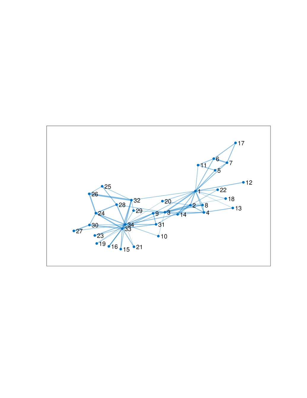
  Fig. 1.1: The graph associated with Zachary’s karate club.

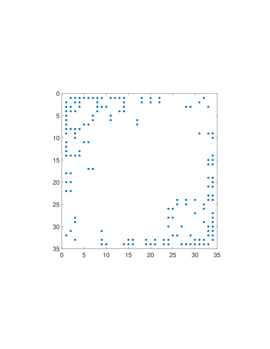
Fig. 1.2: Sparsity pattern of weighted adjacency matrix associated with Zachary’s karate club.

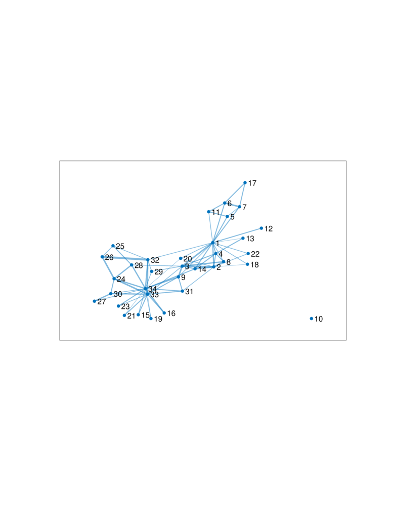
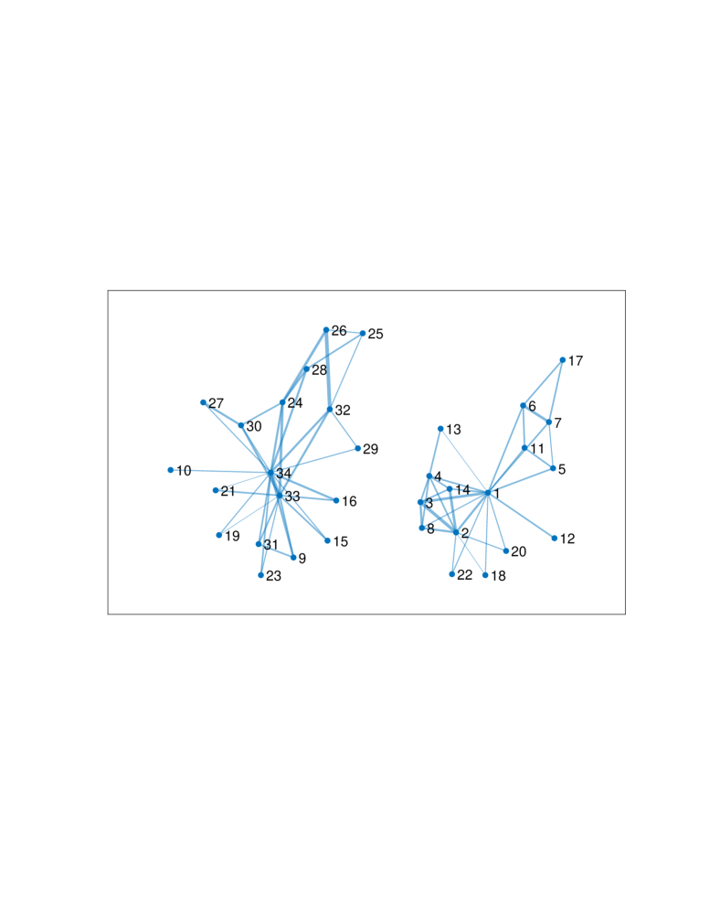
Fig. 1.3: Left: unconstrained minimum cut. Right: cardinality-constrained minimum cut, both for the graph associated with Zachary’s karate club.

• In order to decide where to cut the graph, it is not necessary to compute $\varepsilon_{\star}$ with high accuracy. The iteration can be stopped if, for a given tolerance $\vartheta$, the entries of the vector $v(\varepsilon_{k})$ take only values within two disjoint intervals of width $\vartheta$. This marks the membership to the two connected components.

VIII.1.6 Illustrative examples

We consider a classical test problem of small dimension (Zachary’s karate club). This weighted graph consisting of $34$ vertices; weights describe the relationship between the $34$ members of the karate club; see Zachary (?).

The weights vary in the integer range $[1,7]$. The graph is illustrated in Figure 1.1 where the thickness of the edges increases for larger weights.

The unconstrained minimum cut algorithm determines the graph represented in Figure 1.3, where the graph is cut into two components, one made by the singleton node $\{10\}$ and the other made by the rest of the graph; the value $\varepsilon_{\star}=\sqrt{10}$, which corresponds to the $2$-norm of the $10$-th row of the adjacency matrix multiplied by $2$.

Evidently the result is disappointing, although very predictable, because it does not express a significant clustering of the two communities which attend the Karate club. Note that alternatively also nodes $\{18\}$ and $\{19\}$ might have been cut out since they would have required a cut with the same value.

In order to obtain a meaningful clustering we make use of a cardinality constraint, imposing that each of the two components should have a cardinality of at least $40\%$, that is, the dimension of each cluster should be at least $\lceil 0.4\,n\rceil=14$, where $n=34$.

The result is shown in Figure 1.3 on the right-hand side, which shows two groups of $n_{1}=18$ and $n_{2}=16$ members, respectively. The result has been obtained with a penalty parameter $\alpha=1$, to which corresponds the value $\varepsilon_{\star}=\sqrt{120}=10.95445115..$.

Practical strategy

Numerical experiments seem to indicate that when an active edge is deleted by our algorithm, which means it is set to $0$, then it remains $0$ without reactivating. This suggests an alternative simpler strategy which makes the set of active vertices monotonically decreasing as $\varepsilon$ increases.

A second practical trick consists in terminating the clustering in a combinatorial way. This means that when the functional reaches a value below a certain threshold $\theta$, i.e.

$$\widehat{F}_{\varepsilon}(v)\leq\theta$$

we proceed as follows. We set $B\approx A+\varepsilon E$, where the approximation is obtained, for example, by rounding to the closest integer matrix if the weights are integer or similarly for matrices whose weights are expressed with a $2$-digit fractional part. If $L(B)=0$ then $\varepsilon_{\star}=\|B-A\|_{F}$.

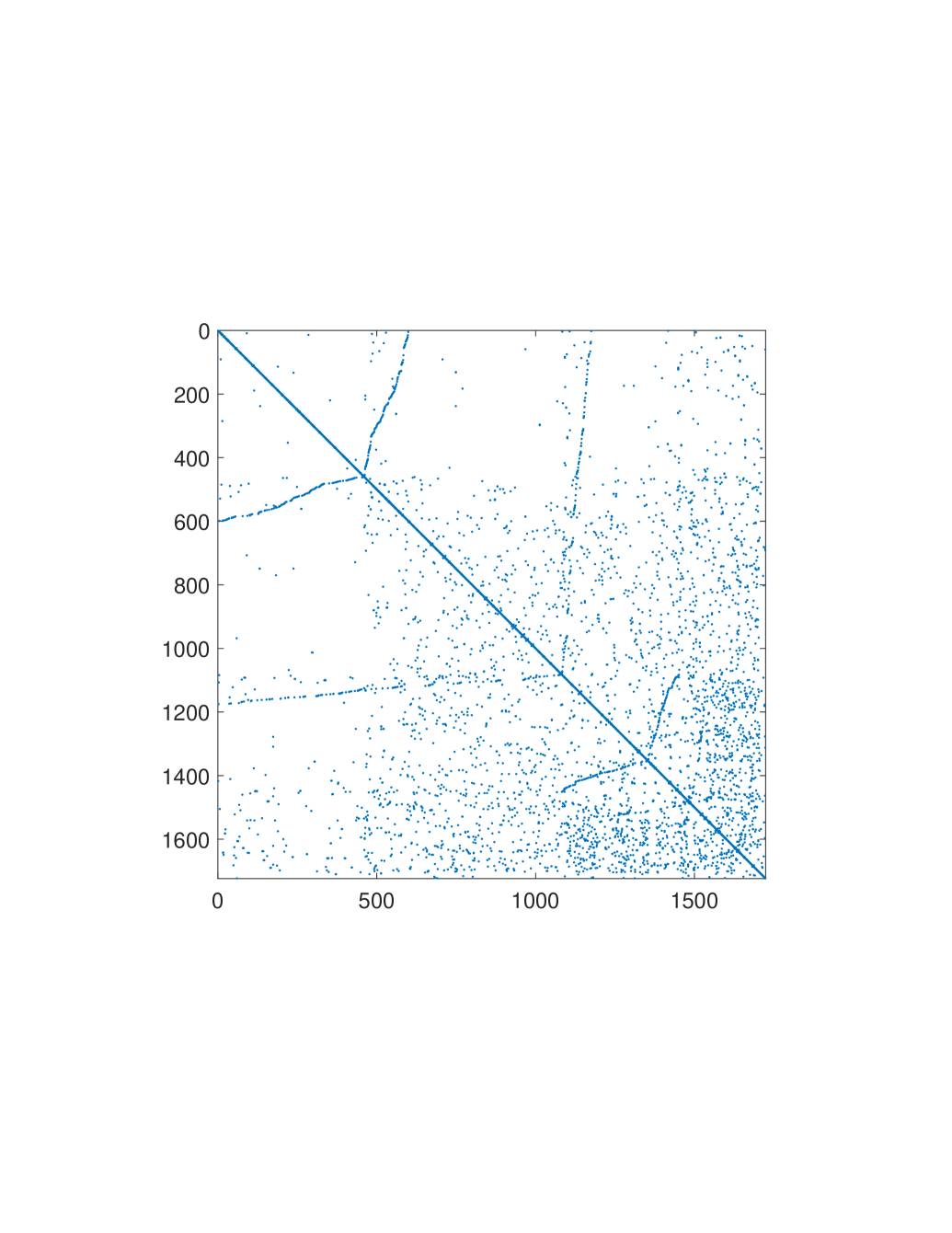
Fig. 1.4: Sparsity pattern of matrix BCSPWR09.

A larger test example

We consider the graph represented by the weighted adjacency matrix BCSPWR09, collected by B. Dembart and J. Lewis, Boeing Computer Services, Seattle, WA, USA.

It consists of a $1723\times 1723$ sparse symmetric matrix, whose sparsity pattern is illustrated in Figure 1.4. All weights are equal to $1$.

The graph is illustrated in Figure 1.5.

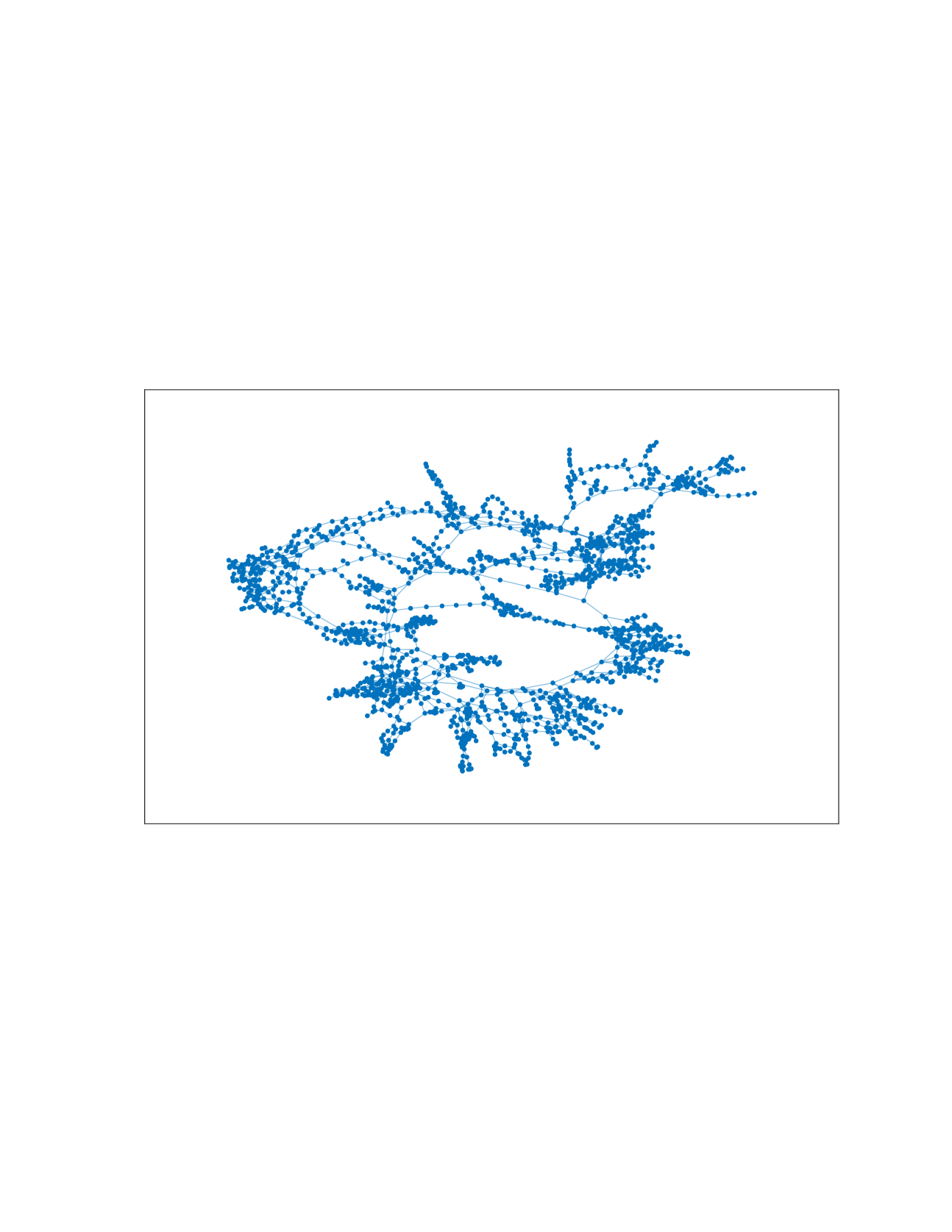
Fig. 1.5: The graph represented by matrix BCSPWR09.

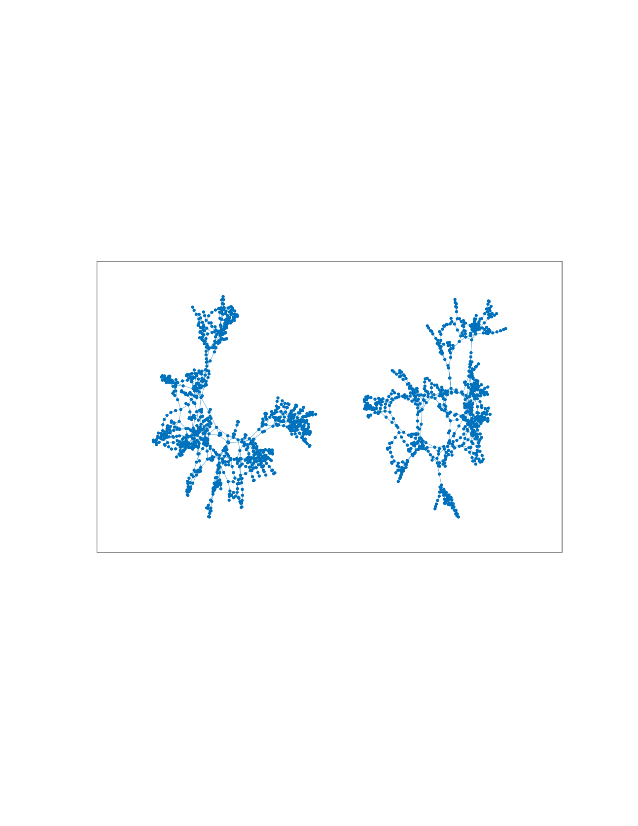
Fig. 1.6: The obtained partition of the graph BCSPWR09, with 10 edges cut.

Setting a cardinality constraint of $40\%$, that is asking for cutting the graph such that each connected subgraph has at least 40% of the nodes, we obtain the two clusters illustrated in Figure 1.6. The graph is illustrated in Figure 1.5.

The two components have cardinality $n_{1}=758$ and $n_{2}=965$ and the computed distance is $\varepsilon_{\star}=\sqrt{20}\approx 4.47213595$. This means that $10$ edges have been cut to provide the splitting.

VIII.2 Toppling the ranking

Which nodes in a graph are important? How to rank their importance? These questions are addressed by the notion of centrality, of which there are several variants. Here we consider eigenvector centrality, which is based on the Perron–Frobenius theorem. The weighted adjacency matrix $A\geq 0$ (with entrywise non-negativity) has a largest, positive real eigenvalue with a non-negative eigenvector $x=(x_{i})\geq 0$. The nodes are ranked according to the entries of this eigenvector:

Node $$i j x_{i}>x_{j}$$ is ranked higher than node if .

In this section we address a basic question: How robust is the ranking under perturbations of the weights $a_{ij}$ in the graph?

• Assume that node 1 is ranked higher than node 2, i.e. $x_{1}>x_{2}$. What is the Frobenius-norm distance to the nearest weighted adjacency matrix $\widetilde{A}\geq 0$ on the same graph such that the ranking of nodes 1 and 2 is reversed, i.e. the Perron–Frobenius eigenvector $\widetilde{x}\geq 0$ of $\widetilde{A}$ has $\widetilde{x}_{1}\leq\widetilde{x}_{2}$?

  We address such questions for undirected graphs (i.e. symmetric $A$) using again computationally inexpensive Rayleigh quotients instead of eigenvalues and eigenvectors and their derivatives. The latter could, however, be used in a similar way also for directed graphs, which cannot be done with Rayleigh quotients.

VIII.2.1 Robustness of ranking as a matrix nearness problem

We consider an undirected graph with vertex set $\mathcal{V}=\{1,\dots,n\}$ and edge set $\widehat{\mathcal{E}}$, and an undirected subgraph with the same vertex set but a possibly reduced edge set $\mathcal{E}\subseteq\widehat{\mathcal{E}}$. We let $\widehat{\mathcal{S}}=\mathrm{Sym}(\widehat{\mathcal{E}})$ and $\mathcal{S}=\mathrm{Sym}(\mathcal{E})$ be the spaces of symmetric real matrices with sparsity pattern given by the edge sets $\widehat{\mathcal{E}}$ and $\mathcal{E}$, respectively. Let $A\in\widehat{\mathcal{S}}$ with $A\geq 0$ be a weighted adjacency matrix of the graph $(\mathcal{V},\widehat{\mathcal{E}})$.

Let $u\in\mathbb{R}^{n}$ be a given nonzero vector. We require that $u$ has entries with positive and negative sign. For Example VIII.2 we would take $u=e_{1}-e_{2}$, where $e_{i}$ is the $i$th standard unit vector. We consider the following matrix nearness problem.

Problem. Find a matrix $\Delta\in\mathcal{S}=\mathrm{Sym}(\mathcal{E})$ of minimal Frobenius norm such that ${A+\Delta\geq 0}$ and the Perron–Frobenius eigenvector $x\geq 0$ of $A+\Delta$ is orthogonal to the given vector $u$.

Note that for Example VIII.2 the orthogonality constraint is

$$0=u^{\top}x=(e_{1}-e_{2})^{\top}x=e_{1}^{\top}x-e_{2}^{\top}x=x_{1}-x_{2},$$

i.e. the orthogonality imposes that nodes 1 and 2 are ranked equally, as opposed to the original ranking $x_{1}>x_{2}$. Choosing $u=1.01\,e_{1}-e_{2}$ would reverse the ranking.

We will propose a two-level approach that does not use eigenvectors and not even eigenvalues in the functional to be minimized. This approach relies on the following lemma.

• (Rayleigh quotients under an orthogonality constraint).  Let $A\in\mathbb{R}^{n,n}$ be a symmetric matrix, and let the nonzero vector $u\in\mathbb{R}^{n}$ be normalized to have Euclidean norm 1. Let $v_{\star}\in\mathbb{R}^{n}$ maximize the Rayleigh quotient $v^{\top}Av\,/\,v^{\top}v$ over all nonzero vectors $v\in\mathbb{R}^{n}$ that are orthogonal to $u$:

  $$v_{\star}^{\top}Av_{\star}=\max_{\|v\|=1,u^{\top}v=0}v^{\top}Av,\qquad\quad\|v_{\star}\|=1,\ \ u^{\top}v_{\star}=0.$$

  Then, the following holds true:

  (a) $v_{\star}$ is an eigenvector to the largest eigenvalue $\lambda_{\star}=v_{\star}^{\top}Av_{\star}$ of $P_{u}^{\perp}AP_{u}^{\perp}$, where $P_{u}^{\perp}=I-P_{u}$ and $P_{u}=uu^{\top}$ is the orthogonal projection onto the span of $u$.

  (b) $v_{\star}$ is an eigenvector of $A$ if and only if

  $$u^{\top}Av_{\star}=0.$$

  In this case, $v_{\star}$ or $u$ is an eigenvector to the largest eigenvalue of $A$.

  • (a) follows directly from the fact that $P_{u}^{\perp}v=v$ for every $v$ orthogonal to $u$. For part (b), after changing to an orthonormal basis of $\mathbb{R}^{n}$ that has $u$ as the first basis vector, we may assume $u=e_{1}$. We partition the matrix $A$ and the vector $v$ orthogonal to $e_{1}$ as

    $$A=\begin{pmatrix}\alpha&a^{\top}\\ a&\check{A}\end{pmatrix},\quad\ v=\begin{pmatrix}0\\ \check{v}\end{pmatrix},\qquad\text{so that}\quad Av=\begin{pmatrix}a^{\top}\check{v}\\ \check{v}\end{pmatrix}.$$

    Hence, $Av=\lambda v$ if and only if

    $$0=a^{\top}\check{v}=e_{1}^{\top}Av=u^{\top}Av\quad\text{ and }\quad\check{A}\check{v}=\lambda\check{v}.$$

    The latter equation is equivalent to $P_{u}^{\perp}AP_{u}^{\perp}v=\lambda v$, since for $u=e_{1}$,

    $$P_{u}^{\perp}AP_{u}^{\perp}=\begin{pmatrix}0&0\\ 0&\check{A}\end{pmatrix}.$$

    By the Courant–Fischer minimax principle, the second-largest eigenvalue $\lambda_{2}$ of $A$ equals

    $$\lambda_{2}=\min_{\mathcal{U}_{1}}\max_{0\neq v\perp\mathcal{U}_{1}}\frac{v^{\top}Av}{v^{\top}v},$$

    where the minimum is over all one-dimensional subspaces $\mathcal{U}_{1}$ of $\mathbb{R}^{n}$ and is attained only for the span of an eigenvector to the largest eigenvalue of $A$. With the particular choice $\mathcal{U}_{1}=\text{span}(u)$ we obtain, unless $u$ is an eigenvector to the largest eigenvalue of $A$,

    $$\lambda_{2}<\max_{0\neq v\perp u}\frac{v^{\top}Av}{v^{\top}v}=v_{\star}^{\top}Av_{\star}=\lambda_{\star},$$

    so that $\lambda_{\star}$ is the largest eigenvalue of $A$ if it is some eigenvalue of $A$.   $\sqcap$$\sqcup$

VIII.2.2 Two-level iteration

Let $A\in\widehat{\mathcal{S}}=\mathrm{Sym}(\widehat{\mathcal{E}})$ with $A\geq 0$ and $u\in\mathbb{R}^{n}$ of norm 1 be given. The choice of the functional in the following two-level approach is motivated by Lemma VIII.2.1. Here, $\lambda_{\max}(M)$ is the largest eigenvalue of a symmetric matrix $M$.

• Inner iteration: Given $\varepsilon>0$, we aim to compute a matrix $E\in\mathcal{S}=\mathrm{Sym}(\mathcal{E})$ of Frobenius norm 1 with $A+\varepsilon E\geq 0$ and a vector $v\in\mathbb{R}^{n}$ of norm 1 and orthogonal to $u$ such that

  $$F_{\varepsilon}(E,v)=\bigl{(}\lambda_{\max}(A+\varepsilon E)-v^{\top}(A+\varepsilon E)v\bigr{)}+\bigl{(}u^{\top}(A+\varepsilon E)v\bigr{)}^{2}$$ (2.1)

  is minimized under the constraints $\|E\|_{F}=1$, $\|v\|=1$, $u^{\top}v=0$ and $A+\varepsilon E\geq 0$. We write

  $$\bigl{(}E(\varepsilon),v(\varepsilon)\bigr{)}=\arg\min\limits_{(E,v)}F_{\varepsilon}(E,v).$$

• Outer iteration: We compute $\varepsilon_{\star}$ as the smallest $\varepsilon>0$ such that $F_{\varepsilon}(E(\varepsilon),v(\varepsilon))=0$.

Lemma VIII.2.1 shows that if this iteration succeeds, then $\Delta=\varepsilon_{\star}E(\varepsilon_{\star})\in\mathcal{S}$ is the matrix of smallest Frobenius norm such that $A+\Delta\geq 0$ has a Perron-Frobenius eigenvector that is orthogonal to $u$, and $v(\varepsilon_{\star})$ (taken with the proper sign) is this eigenvector.

Since the functional $F_{\varepsilon}$ does not involve eigenvectors, the corresponding gradient flow system does not require computing derivatives of eigenvectors. It contains, however, a largest eigenvalue, and therefore the gradient system requires the computation of largest eigenvalues and their eigenvectors of varying matrices $A+\varepsilon E$.

Constrained gradient flow for the inner iteration.

Consider a smooth path of matrices $E(t)\in\mathcal{S}$ and vectors $v(t)\in\mathbb{R}^{n}$, and let $x(t)$ be the eigenvector of $A+\varepsilon E(t)$ to the largest eigenvalue, which is assumed to be a simple eigenvalue. We let $\sigma(t)=2u^{\top}(A+\varepsilon E)v(t)$. Then we find, omitting the argument $t$ on the right-hand side,

$$\frac{d}{dt}F_{\varepsilon}(E(t),v(t)) =\langle\Pi^{\mathcal{S}}(xx^{\top}-vv^{\top}+\sigma uv^{\top}),\varepsilon\dot{E}\rangle$$

$$\quad+\langle-2(A+\varepsilon E)v+\sigma(A+\varepsilon E)u,\dot{v}\rangle.$$ (2.2)

The gradient flow subject to the constraints $E\in\mathcal{S}$, $\|E\|_{F}=1$, $\|v\|=1$ and $u^{\top}v=0$ therefore becomes

$$\varepsilon\dot{E} =-G+\langle G,E\rangle E\qquad\qquad\text{with}\quad G=\Pi^{\mathcal{S}}(xx^{\top}-vv^{\top}+\sigma\,uv^{\top})$$ (2.3)

$$\dot{v} =-g+\langle g,v\rangle v+\langle g,u\rangle u\quad\text{with}\quad g=-2(A+\varepsilon E)v+\sigma(A+\varepsilon E)u.$$

For simplicity, we do not include the nonnegativity constraint $A+\varepsilon E\geq 0$, which can be enforced in the same way as in the previous section.

An approach without computing eigenvalues and eigenvectors.

We modify the above approach, using a Rayleigh quotient instead of the largest eigenvalue. We replace the eigenvalue $\lambda_{\max}(A+\varepsilon E)$ by a Rayleigh quotient $x^{\top}(A+\varepsilon E)x$ (with $\|x\|=1$), where $x(t)$ satisfies the gradient system for maximizing $x^{\top}(A+\varepsilon E)x$ over all $x\in\mathbb{R}^{n}$ of norm 1 without orthogonality constraint: with a time-scaling factor $\rho>0$, we let

$$\rho\dot{x}=(A+\varepsilon E)x-\langle(A+\varepsilon E)x,x\rangle x,$$ (2.4)

ideally starting from the Perron–Frobenius eigenvector to $A+\varepsilon E_{0}$. We combine (2.4) with the differential equations (2.3). We then have the same stationary point $(E(\varepsilon),v(\varepsilon))$ as before, and $x(\varepsilon)$ is the Perron–Frobenius eigenvector of $A+\varepsilon E(\varepsilon)$.

Newton–bisection method for the outer iteration.

As in previous chapters, we use a combined Newton–bisection method to compute $\varepsilon_{\star}$. By the same arguments as in the proof of Theorem IV.IV.1.4 we find that under analogous assumptions the univariate function $\phi(\varepsilon)=F_{\varepsilon}(E(\varepsilon),v(\varepsilon))$ has the derivative

$$\phi^{\prime}(\varepsilon)=-\|G(\varepsilon)\|_{F},$$

where $G(\varepsilon)$ is the gradient matrix $G$ of (2.3) that corresponds to the minimizer $(E(\varepsilon),v(\varepsilon))$. This derivative is used in Newton’s method for solving $\phi(\varepsilon)=0$.

Optimal perturbation.

We show that under plausible assumptions, the matrix nearness problem stated in Section VIII.2.1 has an optimal perturbation $\Delta\in\mathcal{S}$ such that

$$\Delta \Pi^{\mathcal{S}}(uv^{\top}) v\in\mathbb{R}^{n}$$ is a real multiple of a projected rank-1 matrix for some .

Moreover, it turns out that $\pm v$ is then the Perron–Frobenius eigenvector of $A+\Delta$.

To arrive at this result, we consider the minimization of a modification of the functional $F_{\varepsilon}$ in (2.1) in which we take the square root of the second term:

$$F_{\varepsilon}(E,v)=\bigl{(}\lambda_{\max}(A+\varepsilon E)-v^{\top}(A+\varepsilon E)v\bigr{)}+\bigl{|}u^{\top}(A+\varepsilon E)v\bigr{|}.$$

We let $\varepsilon\nearrow\varepsilon_{\star}$, for which the minimum of $F_{\varepsilon_{\star}}$ becomes zero. In the stationary point $(E(\varepsilon),v(\varepsilon))$ of (2.3), $E(\varepsilon)$ is a multiple of

$$G(\varepsilon)=\Pi^{\mathcal{S}}\bigl{(}x(\varepsilon)x(\varepsilon)^{\top}-v(\varepsilon)v(\varepsilon)^{\top}+\sigma(\varepsilon)uv(\varepsilon)^{\top}\bigr{)},$$

where $x(\varepsilon)$ is the Perron–Frobenius eigenvector of $A+\varepsilon E(\varepsilon)$ and the factor $\sigma(\varepsilon)$ is now changed to $\sigma(\varepsilon)=\mathrm{sign}\bigl{(}u^{\top}(A+\varepsilon E(\varepsilon))v(\varepsilon)^{\top}\bigr{)}$.

We assume that $\sigma(\varepsilon)=1$ (or alternatively $-1$) for a sequence of $\varepsilon<\varepsilon_{\star}$ that converges to $\varepsilon_{\star}$. We further assume that $F_{\varepsilon}(E(\varepsilon),v(\varepsilon))\to 0$ as $\varepsilon\nearrow\varepsilon_{\star}$.

By compactness, $(E(\varepsilon),v(\varepsilon))$ has an accumulation point, which then equals a minimizer $(E(\varepsilon_{\star}),v(\varepsilon_{\star}))$ of $F_{\varepsilon_{\star}}$, i.e., $F_{\varepsilon_{\star}}(E(\varepsilon_{\star}),v(\varepsilon_{\star}))=0$. At $\varepsilon_{\star}$ we have $v(\varepsilon_{\star})=x(\varepsilon_{\star})$, and (up to extraction of a subsequence) we have $v(\varepsilon)\to v(\varepsilon_{\star})$ as $\varepsilon\nearrow\varepsilon_{\star}$. This implies $G(\varepsilon)\to G_{*}=\pm\Pi^{\mathcal{S}}\bigl{(}uv(\varepsilon_{\star})^{\top}\bigr{)}$, and since $E(\varepsilon)\to E(\varepsilon_{\star})$ (up to extraction of a subsequence), we have that $E(\varepsilon_{\star})$ is a multiple of $G_{*}$. Since $\Delta=\varepsilon_{\star}E(\varepsilon_{\star})$ is an optimal perturbation, this yields the stated result.

Example: Matrix $A_{27}$.

The considered graph is one of a sequence of graphs arising from molecular dynamics simulations aimed at analyzing the structure of water networks under different temperature and pressure conditions; see Faccio, Benzi, Zanetti-Polzi & Daidone (?). It consists of $710$ nodes (corresponding to oxygen atoms), most of which ($613$) have degree $4$. Its pattern is shown in Figure 2.1.

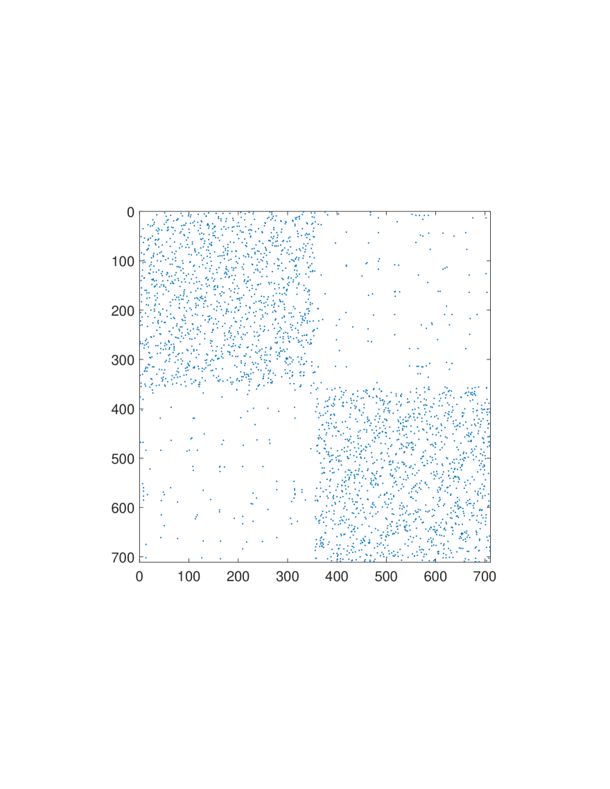
Fig. 2.1: Pattern of the adjacency matrix for the graph example $A_{27}$.

In Figure 2.2 we show the entries of the Perron eigenvector of the original (left picture) and perturbed (right picture).

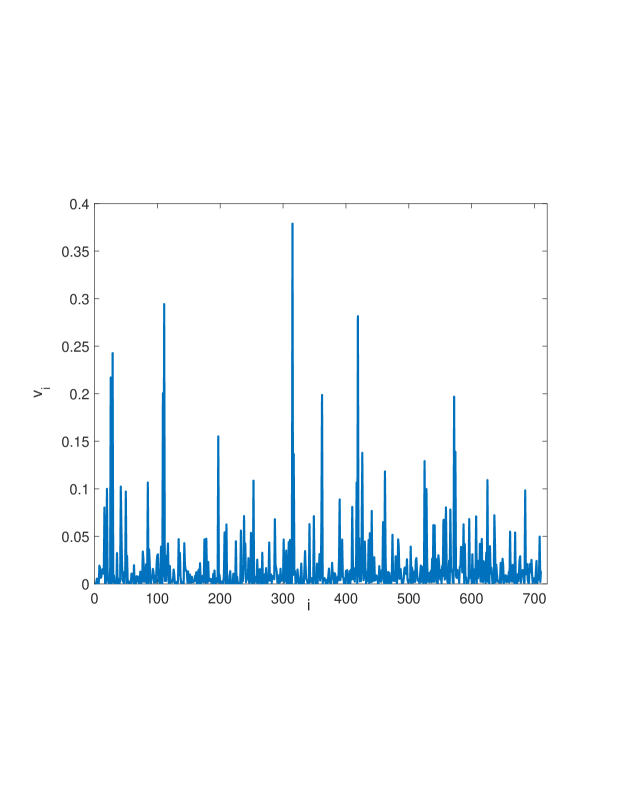
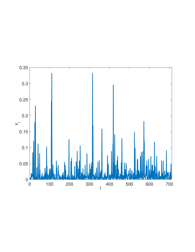
Fig. 2.2: Distribution of the entries of Perron eigenvector for the example $A_{27}$.

The five leading entries of the Perron eigenvector of $A$ are the following:

$$v_{26}=0.21705332,\quad v_{29}=0.24269500,\quad v_{419}=0.28145420,$$

$$v_{111}=0.29422909,\quad v_{315}=0.37879622.$$

After scaling the matrix $A$ to have Frobenius norm $1$, we apply the algorithm. The norm of the perturbation which determines the coalescence of the two main entries of the Perron eigenvector is $\varepsilon_{\star}=0.0092654$, which is below $1\%$. The target vertices are $v_{111}$ and $v_{315}$; after the perturbation they are numerically equal:

$$v_{111}=0.33101615,\qquad v_{315}=0.33136357.$$

The variations of the two entries are $\delta_{111}=+0.1281$ and $\delta_{315}=-0.1235$.

$k$	$\varepsilon_{k}$	$\phi(\varepsilon_{k})$
​​​​ $0$	$0.005$	$0.000375176389506$
$1$	$0.005136626814311$	$0.000351719368954$
$2$	$0.008469968038737$	$0.000013522265277$
$3$	$0.008489282220273$	$0.000012884575588$
$6$	$0.009184673253577$	$0.000000185817345$
$10$	$0.009212325217551$	$0.000000093285281$

Table 2.1: Computation of $\varepsilon_{k}$ and $\phi(\varepsilon_{k})$.

VIII.2.3 Commuting projections: a minimalistic algorithm

We assume in the following that the orthogonal projection $P_{u}=uu^{\top}$ onto the span of $u$ (for $u\in\mathbb{R}^{n}$ of norm 1) and the projection $\Pi^{\mathcal{E}}$ onto the sparsity pattern given by the edge set $\mathcal{E}$ commute. The latter projection is simply, for $Z=(z_{ij})\in\mathbb{R}^{n,n}$,

$$\Pi^{\mathcal{E}}(Z)=\begin{cases}z_{ij},&\text{if }(i,j)\in\mathcal{E}\,,\\ 0\,,&\text{otherwise.}\end{cases}$$

Note that the orthogonal projection $\Pi^{\mathcal{S}}$ onto $\mathcal{S}=\mathrm{Sym}(\mathcal{E})$ as defined in (1.3) is given by $\Pi^{\mathcal{S}}(Z)=\Pi^{\mathcal{E}}(\mathrm{Sym}(Z))$, where $\mathrm{Sym}(Z)=\tfrac{1}{2}(Z+Z^{\top})$ is the symmetric part of $Z\in\mathbb{R}^{n,n}$. We will assume that the projections $P_{u}$ and $\Pi^{\mathcal{E}}$ commute in the following sense:

$$P_{u}\Pi^{\mathcal{E}}(Z)=\Pi^{\mathcal{E}}(P_{u}Z)\quad\text{ and }\quad\Pi^{\mathcal{E}}(Z)P_{u}=\Pi^{\mathcal{E}}(ZP_{u}).$$ (2.5)

In Example VIII.2, this condition is satisfied if with $(1,k)\in\mathcal{E}$ for some $k$, also $(2,k)\in\mathcal{E}$, and conversely. In general, this condition is satisfied if with each $(i,k)\in\mathcal{E}$ with $u_{i}\neq 0$, also $(j,k)\in\mathcal{E}$ for each $j$ with $u_{j}\neq 0$. If the graph $(\mathcal{V},\mathcal{E})$ does not satisfy this condition, then we can extend the edge set in this way and allow for perturbations of weights on the extended graph with the closure of the edge set $\mathcal{E}$ with respect to the fixed vector $u$:

$$\overline{\mathcal{E}}=\mathcal{E}\cup\{(j,k)\text{ and }(k,j)\,:\text{$u_{j}\neq 0$ and $(i,k)\in\mathcal{E}$ for some $i$ with $u_{i}\neq 0$}\}.$$ (2.6)

It will be seen that the commutativity (2.5) leads to a substantial simplification of the problem thanks to orthogonality relations as given in the following lemma.

• (Orthogonality implied by commutativity).  Under the commutativity condition (2.5), we have for all $v\in\mathbb{R}^{n}$ with ${u^{\top}v=0}$

  $$\langle\Pi^{\mathcal{S}}(uv^{\top}),\Pi^{\mathcal{S}}(vv^{\top})\rangle=0.$$

  • Using $P_{u}^{\perp}v=v$ and $P_{u}^{\perp}u=0$ together with (2.5), we find

    $$\langle\Pi^{\mathcal{S}}(uv^{\top}),\Pi^{\mathcal{S}}(vv^{\top})\rangle=\langle\Pi^{\mathcal{S}}(uv^{\top}),vv^{\top}\rangle=v^{\top}\Pi^{\mathcal{S}}(uv^{\top})v$$

    $$=v^{\top}P_{u}^{\perp}\Pi^{\mathcal{S}}(uv^{\top})P_{u}^{\perp}v=v^{\top}P_{u}^{\perp}\Pi^{\mathcal{E}}\bigl{(}\tfrac{1}{2}(uv^{\top}+vu^{\top})\bigr{)}P_{u}^{\perp}v$$

    $$=v^{\top}\Pi^{\mathcal{E}}\bigl{(}\tfrac{1}{2}P_{u}^{\perp}(uv^{\top}+vu^{\top})P_{u}^{\perp}\bigr{)}v=v^{\top}\Pi^{\mathcal{E}}(0)v=0$$

    as stated.   $\sqcap$$\sqcup$

    With this orthogonality we obtain the following partial solution to the problem, ignoring the non-negativity constraint on the perturbed matrix for the moment. A remarkable feature is that the optimal perturbation $\Delta$ is fully characterized by the vector $u$ and the vector $v$ that maximizes the Rayleigh quotient of the original matrix $A$ under the orthogonality constraint $u^{\top}v=0$. Moreover, the perturbation matrix $\Delta$ changes only entries $(i,j)\in\mathcal{E}$ that have $u_{i}\neq 0$ or $u_{j}\neq 0$. In Example VIII.2, only entries in the first two rows and columns of $A$ are changed.

    • (Matrix nearness problem solved without non-negativity constraint).  Let $A\in\mathcal{S}=\mathrm{Sym}(\mathcal{E})$ and $u\in\mathbb{R}^{n}$ of norm $1$ be given. Let $v\in\mathbb{R}^{n}$ be an eigenvector to the largest eigenvalue $\lambda_{u}(A)$ of $P_{u}^{\perp}AP_{u}^{\perp}$, i.e. $v$ maximizes the Rayleigh quotients of $A$ subject to the orthogonality constraint $u^{\top}v=0$. Under the commutativity condition (2.5), the matrix $\Delta$ of smallest Frobenius norm such that an eigenvector to the largest eigenvalue of $A+\Delta$ is orthogonal to the vector $u$, is given by

      $$\Delta=-\vartheta\Pi^{\mathcal{S}}(uv^{\top})\quad\text{with}\quad\vartheta=\frac{u^{\top}Av}{\|\Pi^{\mathcal{S}}(uv^{\top})\|_{F}^{2}}.$$

      Moreover, $v$ is such an eigenvector to the largest eigenvalue of $A+\Delta$, which is still $\lambda_{u}(A)$.

  • For every $v\in\mathbb{R}^{n}$ that is orthogonal to $u$ and every $\vartheta\in\mathbb{R}$ we have $v^{\top}P_{u}^{\perp}AP_{u}^{\perp}v=v^{\top}Av$ and

    $$v^{\top}(A-\vartheta\Pi^{\mathcal{S}}(uv^{\top}))v=v^{\top}Av-\vartheta\langle\Pi^{\mathcal{S}}(uv^{\top}),\Pi^{\mathcal{S}}(vv^{\top})\rangle=v^{\top}Av$$

    by Lemma VIII.2.3. An eigenvector $v$ to the largest eigenvalue of $P_{u}^{\perp}AP_{u}^{\perp}$ is then also an eigenvector to the largest eigenvalue of $P_{u}^{\perp}(A-\vartheta\Pi^{\mathcal{S}}(uv^{\top}))P_{u}^{\perp}$ for every $\vartheta\in\mathbb{R}$.

    On the other hand, we know from above that the matrix $\Delta$ of a given norm that minimizes $|u^{\top}(A+\Delta)v|$, is a multiple of $\Pi^{\mathcal{S}}(uv^{\top})$ as long as the minimum value is positive. By continuity, this remains true also for the smallest norm for which the minimum value becomes zero. We have

    $$u^{\top}(A-\vartheta\Pi^{\mathcal{S}}(uv^{\top}))v=u^{\top}Av-\vartheta\langle\Pi^{\mathcal{S}}(uv^{\top}),uv^{\top}\rangle=u^{\top}Av-\vartheta\|\Pi^{\mathcal{S}}(uv^{\top})\|_{F}^{2},$$

    which is zero for $\vartheta$ as stated in the theorem. For this $\vartheta$, Lemma VIII.2.1 yields that an eigenvector $v\perp u$ to the largest eigenvalue of $P_{u}^{\perp}(A-\vartheta\Pi^{\mathcal{S}}(uv^{\top}))P_{u}^{\perp}$ is an eigenvector to the largest eigenvalue of $A-\vartheta\Pi^{\mathcal{S}}(uv^{\top})$ (unless $u$ is).   $\sqcap$$\sqcup$

Non-negativity constraint.

Theorem VIII.2.3 does not take the non-negativity of the matrix into account. It solves the problem only if $A+\Delta\geq 0$, which may or may not happen.

Algorithm 2.12 aims at reducing $|u^{\top}(A+\Delta)v|$ to zero while respecting the non-negativity constraint $A+\Delta\geq 0$ and retaining the commutativity of projections on subgraphs that exclude those matrix entries that cannot be further changed because of the non-negativity constraint. Note that the reduced edge sets $\mathcal{E}_{k+1}\subset\mathcal{E}_{k}$ are constructed in such a way that $\Pi^{\mathcal{E}_{k+1}}$ still commutes with $P_{u}$.

When the algorithm finishes after finitely many steps, it returns, in the case of success, a perturbation matrix $\Delta$ (expected to be of minimal Frobenius norm but with no proof) that satisfies $A+\Delta\geq 0$ and has the vector $v$ with $u^{\top}v=0$ of Theorem VIII.2.3 as an eigenvector to the largest eigenvalue (assuming it is not $u$). If the largest eigenvalue is simple, then $v$ must be a multiple of the non-negative Perron–Frobenius eigenvector of the non-negative matrix $A+\Delta$. If the algorithm returns with failure, it has reduced $|u^{\top}(A+\Delta)v|$ as far as is feasible with commuting projections.

Data: weighted adjacency matrix $A$, edge set $\mathcal{E}$, vector $u$ of norm 1,

$\qquad v$ eigenvector to the largest eigenvalue of $P_{u}^{\perp}AP_{u}^{\perp}$

Result: perturbation matrix $\Delta$ in the cases of ‘success’ and ‘failure’

begin

   1 Initialize $A_{0}=A$ and $\mathcal{E}_{0}=\{(i,j)\in\overline{\mathcal{E}}\,:\,u_{i}\neq 0\;\text{ or }\,u_{j}\neq 0\}$ (see (2.6))

   2 Initialize $\Theta_{0}=\Pi^{\mathcal{E}_{0}}(\mathrm{Sym}(uv^{\top}))$

   3 Initialize $k=0$  and  flag = ‘ongoing’

    while flag = ‘ongoing’ do

      4 Set $\vartheta_{k}=\displaystyle\frac{u^{\top}A_{k}v}{\|\Theta_{k}\|_{F}^{2}}$

       if $A_{k}-\vartheta_{k}\Theta_{k}\geq 0$ then

         Set $\Delta=A_{k}-\vartheta_{k}\Theta_{k}-A$, flag = ‘success’, return

      5Set $\rho_{k}=\max\{\rho\,:\,A_{k}-\rho\,\mathrm{sign}(\vartheta_{k})\,\Theta_{k}\geq 0\}$

      6 Set $A_{k+1}=A_{k}-\rho_{k}\,\mathrm{sign}(\vartheta_{k})\,\Theta_{k}$

      7 Set $\mathcal{E}_{k+1}^{0}=\{(i,j)\in\mathcal{E}_{k}\,:\,A_{k+1}\big{|}_{i,j}=0\}$

      8 Set $\mathcal{E}_{k+1}=\mathcal{E}_{k}\setminus\overline{\mathcal{E}_{k+1}^{0}}$ (see (2.6))

       if $\mathcal{E}_{k+1}=\emptyset$ then

         Set $\Delta=A_{k+1}-A$, flag = ‘failure’, return

      Set $\Theta_{k+1}=\Pi^{\mathcal{E}_{k+1}}(\Theta_{k})$

       Set $k=k+1$

   

Algorithm 2.12 Iterative reduction preserving non-negativity and commutativity of projections.

VIII.3 Notes

The usefulness of eigenvalues in studying graphs has been explored and amply demonstrated in spectral graph theory; see the book by Chung (?) and the introductory articles by Spielman (?) and von Luxburg (?). In this chapter we put forward an approach that does not use spectral information of a matrix associated with the given graph (the graph Laplacian or the weighted adjacency matrix), but of such matrices for graphs with suitably perturbed weights. We reformulate classical problems in graph theory as matrix nearness problems related to eigenvalue optimization. We then adapt algorithms that we developed in previous chapters, using a two-level iteration with a constrained gradient system in the inner iteration. Such an approach to optimization problems for graphs was first taken by Andreotti, Edelmann, Guglielmi & Lubich (?), for the problem of constrained graph partitioning. Robustness of spectral clustering to perturbations in the weight matrix was subsequently studied in a related setting by Andreotti, Edelmann, Guglielmi & Lubich (?) and Guglielmi & Sicilia (?).

Constrained clustering.

Constrained partitioning of graphs is a varied research area; see e.g. Kamvar, Sepandar, Klein, Dan, Manning, and Christopher (?), Li, Liu & Tang (?), Xu, Li & Schuurmans (?), Wang & Davidson (?), and Bühler, Rangapuram, Setzer & Hein (?). For the classical unconstrained minimum cut problem, there exist algorithms with complexity $O(n^{2}\log n+nm)$ for graphs with $n$ nodes and $m$ edges; see Stoer & Wagner (?) and references therein. However, cardinality constraints make the minimum cut problem NP-hard; see Bruglieri, Maffioli & Ehrgott (?, ?), who also propose a heuristic combinatorial algorithm for the cardinality-constrained minimum cut problem. Must-link and cannot-link constraints were imposed by Wagstaff, Cardie, Rogers & Schrödl (?) and in many works thereafter; see e.g. Basu, Davidson, and Wagstaff (?).

Andreotti, Edelmann, Guglielmi & Lubich (?) formulated constrained graph partitioning as a matrix nearness problem and gave an iterative algorithm using eigenvalues and eigenvectors of the Laplacian of graphs with suitably perturbed weights. The new algorithm presented in Section VIII.1 is similar in spirit but uses instead Rayleigh quotients, which are computationally significantly cheaper.

Robustness of spectral clustering.

The spectral clustering algorithm, see e.g. the review by von Luxburg (?), is widely used for partitioning an undirected graph. Robustness of spectral clustering has been addressed from a statistical viewpoint by von Luxburg (?). In a different direction, asking for the smallest perturbation of the weight matrix on the given graph that changes the partition, yields a matrix nearness problem that has first been studied by Andreotti, Edelmann, Guglielmi & Lubich (?). They devise a two-level iteration that uses a constrained gradient system in the inner iteration. This has been taken further by Guglielmi & Sicilia (?), where the inner iteration works with projected rank-1 perturbation matrices similarly to the rank-1 approach in Chapter V. We can directly refer to the algorithms of those two papers and therefore this topic is not included as a separate section in this chapter.

Robustness of ranking.

Ranking the nodes of a graph via the leading eigenvector can be traced back to Landau (?). After being rediscovered many times, it became widely known through the Google PageRank algorithm; see e.g. Bryan & Leise (?). Assessing the robustness of a ranking can be viewed as a matrix nearness problem related to eigenvalue and eigenvector optimization. Based on this interpretation, an algorithm for quantifying the robustness of the ranking of nodes — and simultaneously, for changing the ranking by a minimal perturbation — in a given directed or undirected weighted graph was given by Benzi & Guglielmi (?), minimizing a functional of the leading eigenvector. The algorithms for undirected graphs in Section VIII.2 are new and do not require to compute eigenvalues and eigenvectors and their derivatives but work instead with Rayleigh quotients. Related problems have been considered in the literature by other authors. Most relevant to our work are the papers by Cipolla, Durastante and Meini (?) and by Gillis and Van Dooren (?).

Topological stability of simplicial complexes.

Finally, let us mention an application to topological stability of simplicial complexes with respect to perturbations of the underlying graph structure, where a gradient system approach (similar to that considered in this chapter) is applied to the Hodge Laplacian of a weighted simplicial complex to determine the minimal perturbation of edge weights sufficient to create an additional k-dimensional hole; see Guglielmi, Savostianov and Tudisco (?).

Chapter IX Appendix: Derivatives of eigenvalues and eigenvectors

In this appendix we put together a few basic results concerning first order perturbation theory of eigenvalues and eigenvectors. We refer to Greenbaum, Li & Overton (?) for a recent review, which also traces the rich history of this subject area.

IX.1 Derivative of paths of simple eigenvalues

We often use the following standard perturbation result for eigenvalues; see e.g. Horn & Johnson (?), Lemma 6.3.10 and Theorem 6.3.12, and Greenbaum, Li & Overton (?), Theorem 1.

• (Derivative of simple eigenvalues).  Consider a continuously differentiable path of square complex matrices $A(t)$ for $t$ in an open interval $I$. Let $\lambda(t)$, $t\in I$, be a continuous path of simple eigenvalues of $A(t)$. Let $x(t)$ and $y(t)$ be left and right eigenvectors, respectively, of $A(t)$ to the eigenvalue $\lambda(t)$. Then, $x(t)^{*}y(t)\neq 0$ for $t\in I$ and $\lambda$ is continuously differentiable on $I$ with the derivative (denoted by a dot)

  $$\dot{\lambda}=\frac{x^{*}\dot{A}y}{x^{*}y}\,.$$ (1.1)

  Moreover, “continuously differentiable” can be replaced with “analytic” in the assumption and the conclusion. Since we have $x(t)^{*}y(t)\neq 0$, we can apply the normalization

  $$\|x(t)\|=1,\ \ \|y(t)\|=1,\quad x(t)^{*}y(t)\text{ is real and positive.}$$ (1.2)

  Clearly, a pair of left and right eigenvectors $x$ and $y$ fulfilling (1.2) may be replaced by $\mu y$ and $\mu x$ for any complex $\mu$ of modulus $1$ without changing the property (1.2).

  Next we turn to singular values. The following result is obtained from Theorem IX.1 by using the equivalence between singular values of $M$ and eigenvalues of $(0~M;M^{*}~0)$; see Horn & Johnson (?), Theorem 7.3.7.

  • (Derivative of singular values).  Consider a continuously differentiable path of matrices $M(t)\in\mathbb{C}^{m,n}$ for $t$ in an open interval $I$. Let $\sigma(t)$, $t\in I$, be a path of simple singular values of $M(t)$. Let $u(t)$ and $v(t)$ be left and right singular vectors of $M(t)$ to the singular value $\sigma(t)$, that is, $M(t)v(t)=\sigma(t)u(t)$ and $u(t)^{*}M(t)=\sigma(t)v(t)^{*}$ with $\|u(t)\|=\|v(t)\|=1$. Then, $\sigma$ is differentiable on $I$ with the derivative

    $$\dot{\sigma}={\mbox{\rm Re}}(u^{*}\dot{M}v).$$

IX.2 Derivative of paths of eigenvectors

For the derivative of eigenvectors we need the notion of group inverse (or reduced resolvent); see Meyer & Stewart (?) as well as Kato (?), Section I.5.3.

• (Group inverse).  Let $N\in{\mathbb{C}}^{n,n}$ be a singular matrix with a simple zero eigenvalue. The group inverse (or reduced resolvent) of $N$ is the unique matrix $Z$ with

  $$NZ=ZN,\qquad ZNZ=Z,\quad\mbox{and}\quad NZN=N.$$ (2.1)

  For the left and right eigenvectors $x$ and $y$ associated with the eigenvalue $0$ of $N$, these equations yield the useful relations

  $$Zy=ZNZy=Z^{2}Ny=0\quad\text{ and analogously }\quad x^{*}Z=0.$$ (2.2)

  It is known from Meyer & Stewart (?) that if $N$ is normal, then its group inverse $Z$ is equal to the better known Moore–Penrose pseudoinverse $N^{\dagger}$. In general, the two pseudoinverses are not the same. They are, however, related by the following result, which is a special case of a more general result in Appendix A of Guglielmi, Overton & Stewart (?) but is also simply verified directly.

  • (Group inverse via Moore–Penrose pseudoinverse).  Suppose that the matrix $N$ has the simple eigenvalue $0$ with corresponding left and right eigenvectors $x$ and $y$ of unit norm and such that $x^{*}y>0$. Let $Z$ be the group inverse of $N$, and with $\kappa=1/(x^{*}y)$ define the projection $\Pi=I-\kappa yx^{*}$. Then, the group inverse $Z$ of $N$ is related to the Moore–Penrose pseudoinverse $N^{\dagger}$ by

    $$Z=\Pi N^{\dagger}\Pi.$$ (2.3)

    The Moore-Penrose pseudo-inverse $N^{\dagger}$ is obtained from the singular value decomposition $N=U\Sigma V^{*}$ with unitary matrices $U$ and $V$ and the diagonal matrix $\Sigma=(\Sigma_{+}\ 0;\,0\ 0)$, where $\Sigma_{+}$ is the diagonal matrix of the positive singular values. Then, $N^{\dagger}=V\Sigma^{\dagger}U^{*}$, where $\Sigma^{\dagger}=((\Sigma_{+})^{-1}\ 0;\,0\ 0)$. It is then a simple exercise to verify that $\Pi N^{\dagger}\Pi$ satisfies the conditions (2.1) that define the group inverse $Z$. In particular, we find $NZ=ZN=\Pi$, which implies the other two conditions.

  The group inverse appears in the following result on the derivative of eigenvectors, which is a variant of Theorem 2 of Meyer & Stewart (?).

  • (Derivative of eigenvectors). Consider an analytic path of square complex matrices $A(t)$ for $t$ in an open interval $I$. Let $\lambda(t)$, $t\in I$, be a path of simple eigenvalues of $A(t)$. Then, there exists a continuously differentiable path of associated left and right eigenvectors $x(t)$ and $y(t)$, $t\in I$, which are of unit norm with $x^{*}(t)y(t)>0$ and satisfy the differential equations

    $$\begin{array}[]{rcl}\dot{x}^{*}\!\!\!&=&\!\!-x^{*}\dot{A}Z+{\mbox{\rm Re}}(x^{*}\dot{A}Zx)x^{*},\\ \dot{y}&=&\!\!-Z\dot{A}y\ \ +{\mbox{\rm Re}}(y^{*}Z\dot{A}y)y,\end{array}$$ (2.4)

    where $Z(t)$ is the group inverse of $A(t)-\lambda(t)I$.

    We note that the last terms on the right-hand sides of (2.4) are in the direction of $x^{*}$ and $y$. They serve to ensure that the unit norm of $x(t)$ and $y(t)$ is conserved and that $x(t)^{*}y(t)$ remains real (and hence positive by Theorem IX.1). This is shown by verifying that $(d/dt)(x^{*}y)$ is real and that $(d/dt)\|x\|^{2}=2\,{\mbox{\rm Re}}\,\dot{x}^{*}x$ and $(d/dt)\|y\|^{2}=2\,{\mbox{\rm Re}}\,y^{*}\dot{y}$ vanish, using the relations (2.2).

    In Theorem 2 of Meyer & Stewart (?), the last terms in (2.4) appear without taking the real part. While this preserves the unit norm of the left and right eigenvectors, the positivity of their inner product is then not conserved. Dropping the last terms (which are not analytic) altogether yields an analytic path of non-normalized left and right eigenvectors $x^{*}(t)$ and $y(t)$ with constant inner product $x^{*}(t)y(t)$; see Greenbaum, Li & Overton (?), Theorem 2 and Section 3.4.

References

- [2008] P.-A. Absil, R, Mahony and R. Sepulchre. Optimization algorithms on matrix manifolds. Princeton University Press, Princeton, NJ, 2008. \@MHitem
- [2010] S. S. Ahmad, R. Alam, and R. Byers. On pseudospectra, critical points, and multiple eigenvalues of matrix pencils. SIAM J. Matrix Anal. Appl., 31(4): 1915–1933, 2010. \@MHitem
- [2014] R. O. Akinola, M. A. Freitag, and A. Spence. The calculation of the distance to a nearby defective matrix. Numer. Linear Algebra Appl., 21(3): 403–414, 2014. \@MHitem
- [2005] R. Alam and S. Bora. On sensitivity of eigenvalues and eigendecompositions of matrices. Linear Algebra Appl., 396: 273–301 (2005). \@MHitem
- [2011] R. Alam, S. Bora, R. Byers, and M. L. Overton. Characterization and construction of the nearest defective matrix via coalescence of pseudospectral components. Linear Algebra Appl., 435(3): 494–513, 2011. \@MHitem
- [2011] R. Alam, S. Bora, M. Karow, V. Mehrmann, and J. Moro. Perturbation theory for Hamiltonian matrices and the distance to bounded-realness. SIAM J. Matrix Anal. Appl., 32(2): 484–514, 2011. \@MHitem
- [2019] E. Andreotti, D. Edelmann, N. Guglielmi, and C. Lubich. Constrained graph partitioning via matrix differential equations. SIAM J. Matrix Anal. Appl., 40(1): 1–22, 2019. \@MHitem
- [2021] E. Andreotti, D. Edelmann, N. Guglielmi, and C. Lubich. Measuring the stability of spectral clustering. Linear Algebra Appl., 610: 673–697, 2021. \@MHitem
- [1973] B. Anderson and S. Vongpanitlerd. Network Analysis and Synthesis: A Modern Systems Approach Pearson Prentice Hall. 542 p, 1973.
- [2007] P.J. Antsaklis and A.N. Michel. A linear systems primer Birkhäuser Boston Inc, 2007, pages = xvi+517. \@MHitem
- [2020] P. Apkarian and D. Noll. Optimizing the Kreiss constant. SIAM J. Control Optim., 58(6): 3342–3362, 2020. \@MHitem
- [2008] S. Basu, I. Davidson, and K. Wagstaff. Constrained Clustering: Advances in Algorithms, Theory, and Applications. Chapman & Hall/CRC, 2008. \@MHitem
- [2001] C. Bekas and E. Gallopoulos. Cobra: parallel path following for computing the matrix pseudospectrum. Parallel Comput., 27(14): 1879–1896, 2001. \@MHitem
- [2018] P. Benner, R. Lowe, and M. Voigt. -norm computation for large-scale descriptor systems using structured iterative eigensolvers. Numer. Algebra Control Optim., 8(1):119–133, 2018. \@MHitem
- [2015] P. Benner, P. Losse, V. Mehrmann, and M. Voigt. Numerical linear algebra methods for linear differential-algebraic equations. In Surveys in differential-algebraic equations III, 117–175. Springer, Cham. 2015. \@MHitem
- [1999] P. Benner, V. Mehrmann, V. Sima, S. Van Huffel, and A. Varga. SLICOT–A subroutine library in systems and control theory. In Applied and computational control, signals, and circuits, 499–539. Birkhäuser, Boston, MA. 1999. \@MHitem
- [2019] P. Benner & T. Mitchell. Extended and improved criss-cross algorithms for computing the spectral value set abscissa and radius. SIAM J. Matrix Anal. Appl., 40(4): 1325–1352, 2019. \@MHitem
- [2014] P. Benner and M. Voigt. A structured pseudospectral method for -norm computation of large-scale descriptor systems. Math. Control Signals Systems, 26(2):303–338, 2014. \@MHitem
- [2025] M. Benzi and N. Guglielmi. Changing the ranking in eigenvector centrality of a weighted graph by small perturbations. arXiv preprint arXiv:2501.10745, 2025. \@MHitem
- [2012] J. W. Beyn. An integral method for solving nonlinear eigenvalue problems. Linear Alg. Appl., 436(10): 3839–3863, 2012. \@MHitem
- [1990] S. Boyd and V. Balakrishnan. A regularity result for the singular values of a transfer matrix and a quadratically convergent algorithm for computing its -norm. Systems Control Lett., 15: 1–7, 1990. \@MHitem
- [1989] S. Boyd, V. Balakrishnan, and P. Kabamba. A bisection method for computing the norm of a transfer matrix and related problems. Math. Control Signals Systems, 2(3): 207–219, 1989. \@MHitem
- [1990] N.A. Bruinsma and M. Steinbuch. A fast algorithm to compute the -norm of a transfer function matrix. Systems Control Letters, 14:287–293, 1990. \@MHitem
- [2006] M. Bruglieri, M. Ehrgott, H. W. Hamacher, and F. Maffioli. An annotated bibliography of combinatorial optimization problems with fixed cardinality constraints. Discrete Appl. Math., 154(9):1344–1357, 2006. \@MHitem
- [2004] M. Bruglieri, F. Maffioli, and M. Ehrgott. Cardinality constrained minimum cut problems: Complexity and algorithms. Discrete Appl. Math., 137(3):311–341, 2004. \@MHitem
- [1996] M. Brühl. A curve tracing algorithm for computing the pseudospectrum. BIT, 36(3): 441–454, 1996. \@MHitem
- [1990] N. A. Bruinsma and M. Steinbuch. A fast algorithm to compute the -norm of a transfer function matrix. Systems Control Lett., 14: 287–293, 1990. \@MHitem
- [1994] R.P. Braatz, P.M. Young, J.C. Doyle, and M. Morari. Computational complexity of calculation. IEEE Trans. Automat. Control, 39:1000–1002, 1994. \@MHitem
- [2013] T. Brüll and C. Schröder. Dissipativity enforcement via perturbation of para-Hermitian pencils. IEEE Trans. Circuits and Systems I: Regular Papers, 60(1):164–177, 2012. \@MHitem
- [2006] K. Bryan and T. Leise. The $25,000,000,000 eigenvector: The linear algebra behind Google. SIAM Rev., 48(3): 569–581, 2006. \@MHitem
- [2013] T. Bühler, S. S. Rangapuram, S. Setzer, and M. Hein. Constrained fractional set programs and their application in local clustering and community detection. In International Conference on Machine Learning, 624–632, 2013. \@MHitem
- [2003] J. V. Burke, A. S. Lewis, and M. L. Overton. Robust stability and a criss-cross algorithm for pseudospectra. IMA J. Numer. Anal., 23(3): 359–375, 2003. \@MHitem
- [2012] P. Buttà, N. Guglielmi, and S. Noschese, Computing the structured pseudospectrum of a Toeplitz matrix and its extreme points. SIAM J. Matrix Anal. Appl., 33(4): 1300–1319, 2012. \@MHitem
- [1988] R. Byers. A bisection method for measuring the distance of a stable matrix to the unstable matrices. SIAM J. Sci. Statist. Comput., 9(5): 875–881, 1988. \@MHitem
- [1988] R. Byers and N. K. Nichols. On the stability radius of a generalized state-space system. Linear Algebra Appl., 188/189: 113–134, 1993. \@MHitem
- [1998] R. Byers, C. He, and V. Mehrmann. Where is the nearest non-regular pencil? Linear Algebra Appl., 285(1–3): 81–105, 1998. \@MHitem
- [2022] G. Ceruti and Lubich. An unconventional robust integrator for dynamical low-rank approximation. BIT, 62(1): 23–44, 2022. \@MHitem
- [2017] W. Chen, S. K. Özdemir, G. Zhao, J. Wiersig, and L. Yang. Exceptional points enhance sensing in an optical microcavity. Nature, 548(7666): 192–196, 2017. \@MHitem
- [2020] N. Choudhary, N. Gillis and P. Sharma. On approximating the nearest -stable matrix. Numer. Linear Algebra Appl., 27(3): e2282, 13 pp., 2020. \@MHitem
- [1996a] J. Chen, M.K.H. Fan, and C.N. Nett. Structured singular values with nondiagonal structures. I. Characterizations. IEEE Trans. Automat. Control, 41:1507–1511, 1996. \@MHitem
- [1996b] J. Chen, M.K.H. Fan, and C.N. Nett. Structured singular values with nondiagonal structures. II. Computation. IEEE Trans. Automat. Control, 41:1511–1516, 1996. \@MHitem
- [1997] F. R. K. Chung. Spectral graph theory. American Mathematical Soc., 1997. \@MHitem
- [2024] S. Cipolla, F. Durastante, and B. Meini, Enforcing Katz and PageRank Centrality Measures in Complex Networks. arXiv:2409.02524v1, 2024. \@MHitem
- [1980] J. B. Conway and P. R. Halmos. Finite-dimensional points of continuity of Lat. Linear Algebra Appl., 31, 93–102, 1980. \@MHitem
- [2017] F. E. Curtis, T. Mitchell and M. L. Overton. A BFGS-SQP method for nonsmooth, nonconvex, constrained optimization and its evaluation using relative minimization profiles. Optim. Methods Softw., 32(1): 148–181, 2017. \@MHitem
- [2023] B. Das and S. Bora. Nearest rank deficient matrix polynomials. Linear Algebra Appl., 674: 304–350, 2023.
- [2007] E. B. Davies. Linear operators and their spectra. Cambridge Studies in Advanced Mathematics, vol. 106. Cambridge University Press, Cambridge, 2007. \@MHitem
- [1987] J. W. Demmel. On condition numbers and the distance to the nearest ill-posed problem. Numer. Math., 51: 251–289, 1987. \@MHitem
- [2023] F. Dopico, V. Noferini, and L. Nyman. A Riemannian optimization method to compute the nearest singular pencil. arXiv preprint arXiv:2308.12781, 2023. \@MHitem
- [1997] J. L. M. van Dorsselaer. Pseudospectra for matrix pencils and stability of equilibria. BIT, 37(4): 833–845, 1997. \@MHitem
- [1993] J. L. M. van Dorsselaer, J. F. B. M. Kraaijevanger, and M. N. Spijker. Linear stability analysis in the numerical solution of initial value problems. Acta numerica, 1993, 199–237, Acta Numer., Cambridge Univ. Press, Cambridge, 1993. \@MHitem
- [1936] C. Eckart and G. Young. The approximation of one matrix by another of lower rank. Psychometrika, 1: 211–218, 1936. \@MHitem
- [2010] T. Eisner. Stability of operators and operator semigroups. Operator Theory: Advances and Applications, Vol. 209. Birkhäuser, Basel, 2010. \@MHitem
- [2022] C. Faccio, M. Benzi, L. Zanetti-Polzi, and I. Daidone. Low-and high-density forms of liquid water revealed by a new medium-range order descriptor. J. Molecular Liquids, 355:118922, 2022. \@MHitem
- [2021] A. Fazzi, N. Guglielmi and C. Lubich. Finding the nearest passive or nonpassive system via Hamiltonian eigenvalue optimization. SIAM J. Matrix Anal. Appl., 42(4): 1553–1580, 2021. \@MHitem
- [1973] M. Fiedler. Algebraic connectivity of graphs. Czechoslovak Math. J., 23(98): 298–305, 1973. \@MHitem
- [2011] M. A. Freitag and A. Spence. A Newton-based method for the calculation of the distance to instability. Linear Algebra Appl., 435(12): 3189–3205, 2011. \@MHitem
- [2014] M. A. Freitag and A. Spence. A new approach for calculating the real stability radius. BIT, 54(2): 381–400, 2014. \@MHitem
- [1991] M.K.H. Fan, A.L. Tits, and J.C. Doyle. Robustness in the presence of mixed parametric uncertainty and unmodeled dynamics. IEEE Trans. Automat. Control, 36:25–38, 1991. \@MHitem
- [1959] F. R. Gantmacher. Theory of Matrices. Chelsea, New York, 1959. \@MHitem
- [2017] M. Giesbrecht, J. Haraldson, and G. Labahn. Computing the nearest rank-deficient matrix polynomial. Proceedings of the 2017 ACM International Symposium on Symbolic and Algebraic Computation, 181–188, 2017. \@MHitem
- [2019] N. Gillis, M. Karow and P. Sharma. Approximating the nearest stable discrete-time system. Linear Algebra Appl., 573, 37–53, 2019. \@MHitem
- [2018] N. Gillis, V. Mehrmann, and P. Sharma. Computing the nearest stable matrix pairs. Numer. Linear Algebra Appl., 25(5): e2153, 2018.
- [2017] N. Gillis and P. Sharma. On computing the distance to stability for matrices using linear dissipative Hamiltonian systems. Automatica J. IFAC, 85: 113–121, 2017. \@MHitem
- [2018] N. Gillis and P. Sharma. Finding the nearest positive-real system. SIAM J. Numer. Anal., 56(2):1022–1047, 2018. \@MHitem
- [2024] N. Gillis and P. Van Dooren, Assigning Stationary Distributions to Sparse Stochastic Matrices. SIAM J. Matrix. Anal. Appl., 45(4):2184–2210, 2024. \@MHitem
- [2023] M. Gnazzo and N. Guglielmi. On the numerical approximation of the distance to singularity for matrix-valued functions. https://arxiv.org/abs/2309.01220, 2023. \@MHitem
- [2006] S. Graillat, A note on structured pseudospectra. J. Comput. Appl. Math., 191(1), 68–76, 2006. \@MHitem
- [2020] A. Greenbaum, R.-C. Li, and M. L. Overton. First-order perturbation theory for eigenvalues and eigenvectors. SIAM Rev., 62(2): 463–482, 2020. \@MHitem
- [2004] S. Grivet-Talocia. Passivity enforcement via perturbation of Hamiltonian matrices. IEEE Trans. Circuits and Systems I: Regular Papers, 51(9):1755–1769, 2004. \@MHitem
- [2015] S. Grivet-Talocia and B. Gustavsen. Passive macromodeling: Theory and applications. John Wiley & Sons, 2015. \@MHitem
- [2016] N. Guglielmi. On the method by Rostami for computing the real stability radius of large and sparse matrices. SIAM J. Sci. Comput., 38(3): A1662–A1681, 2016. \@MHitem
- [2013] N. Guglielmi, M. Gürbüzbalaban, and M. L. Overton. Fast approximation of the norm via optimization over spectral value sets. SIAM J. Matrix Anal. Appl., 34(2): 709–737, 2013. \@MHitem
- [2014] N. Guglielmi, D. Kressner, and C. Lubich. Computing extremal points of symplectic pseudospectra and solving symplectic matrix nearness problems. SIAM J. Matrix Anal. Appl., 35(4): 1407–1428, 2014. \@MHitem
- [2015] N. Guglielmi, D. Kressner, and C. Lubich. Low rank differential equations for Hamiltonian matrix nearness problems. Numer. Math., 129(2): 279–319, 2015. \@MHitem
- [2011] N. Guglielmi and C. Lubich. Differential equations for roaming pseudospectra: paths to extremal points and boundary tracking. SIAM J. Numer. Anal., 49: 1194–1209, 2011. \@MHitem
- [2012] N. Guglielmi and C. Lubich. Erratum/addendum: Differential equations for roaming pseudospectra: paths to extremal points and boundary tracking. SIAM J. Numer. Anal., 50: 977–981, 2012. \@MHitem
- [2013] N. Guglielmi and C. Lubich. Low-rank dynamics for computing extremal points of real pseudospectra. SIAM J. Matrix Anal. Appl., 34(1): 40–66, 2013. \@MHitem
- [2017] N. Guglielmi and C. Lubich. Matrix stabilization using differential equations. SIAM J. Numer. Anal., 55(6): 3097–3119, 2017. \@MHitem
- [2024] N. Guglielmi and C. Lubich. Transient dynamics under structured perturbations: bridging unstructured and structured pseudospectra. arXiv preprint arXiv:2401.09601, 2024. \@MHitem
- [2017] N. Guglielmi, C. Lubich, and V. Mehrmann. On the nearest singular matrix pencil. SIAM J. Matrix Anal. Appl., 38(3): 776–806, 2017. \@MHitem
- [2023] N. Guglielmi, C. Lubich, and S. Sicilia. Rank-1 matrix differential equations for structured eigenvalue optimization. SIAM J. Numer. Anal., 61: 1737–1762, 2023. \@MHitem
- [2015] N. Guglielmi and M. Manetta. Approximating real stability radii. IMA J. Numer. Anal., 35(3): 1402–1425, 2015. \@MHitem
- [2011] N. Guglielmi and M. L. Overton. Fast algorithms for the approximation of the pseudospectral abscissa and pseudospectral radius of a matrix. SIAM J. Matrix Anal. Appl., 32(4): 1166–1192, 2011. \@MHitem
- [2015] N. Guglielmi, M. L. Overton, and G.W. Stewart. An efficient algorithm for computing the generalized null space decomposition. SIAM J. Matrix Anal. Appl., 36(1): 38–54, 2015. \@MHitem
- [2018] N. Guglielmi and V. Yu. Protasov. On the closest stable/unstable nonnegative matrix and related stability radii. SIAM J. Matrix Anal. Appl., 39(4): 1642–1669, 2018. \@MHitem
- [2017] N. Guglielmi, Mutti-Ur Rehman and D. Kressner. A novel iterative method to approximate structured singular values. SIAM J. Matrix Anal. Appl., 38(2): 361–386, 2017. \@MHitem
- [2023] N. Guglielmi, A, Savostianov and F. Tudisco. Quantifying the structural stability of simplicial homology. J. Sci. Comput., 97(1):25 pages, 2023. \@MHitem
- [2024] N. Guglielmi, and S. Sicilia. (2024). A low-rank ode for spectral clustering stability. Linear Algebra Appl. \@MHitem
- [2000] M. Gu. New methods for estimating the distance to uncontrollability. SIAM J. Matrix Anal. Appl., 21(3): 989–1003 (2000). \@MHitem
- [2006] M. Gu, E. Mengi, M. Overton, J. Xia, and J. Zhu. Fast methods for estimating the distance to uncontrollability. SIAM J. Matrix Anal. Appl., 28(2): 477–502 (2006). \@MHitem
- [2017] S. Güttel and F. Tisseur. The nonlinear eigenvalue problem. Acta Numerica, 26: 1–94, 2017. \@MHitem
- [1999] C. He and G.A. Watson. An algorithm for computing the distance to instability. SIAM J. Matrix Anal. Appl., 20(1): 101–116 (1999). \@MHitem
- [1989] N. J. Higham. Matrix nearness problems and applications. Applications of matrix theory (Bradford, 1988), 1–27, Inst. Math. Appl. Conf. Ser. New Ser., 22, Oxford Univ. Press, New York, 1989. \@MHitem
- [1993] D. Hinrichsen and B. Kelb. Spectral value sets: a graphical tool for robustness analysis. Systems Control Lett., 21(2): 127–136, 1993. \@MHitem
- [1989] D. Hinrichsen, B. Kelb and A. Linnemann. An algorithm for the computation of the structured complex stability radius. Automatica J. IFAC, 25(5): 771–775, 1989. \@MHitem
- [1986a] D. Hinrichsen and A. J. Pritchard. Stability radii of linear systems. Systems Control Lett., 7(1): 1–10, 1986. \@MHitem
- [1986b] D. Hinrichsen and A. J. Pritchard. Stability radius for structured perturbations and the algebraic Riccati equation. Systems Control Lett., 8(2): 115–113, 1986. \@MHitem
- [1990] D. Hinrichsen and A. J. Pritchard. Real and complex stability radii: a survey. Control of uncertain systems (Bremen, 1989), 119–162, Progr. Systems Control Theory, 6, Birkhäuser, Boston, MA, 1990. \@MHitem
- [2005] D. Hinrichsen and A. J. Pritchard. Mathematical systems theory I: modelling, state space analysis, stability and robustness. Springer, Berlin, 2005. \@MHitem
- [1990] R. A. Horn and C. R. Johnson. Matrix Analysis. Cambridge University Press, Cambridge, 1990. Corrected reprint of the 1985 original. \@MHitem
- [1966] W. Kahan. Numerical linear algebra. Canadian Mathematical Bulletin, 9(5): 757–801, 1966. \@MHitem
- [1963] R. E. Kalman. Mathematical description of linear dynamical systems. J. SIAM Control Ser. A, 1: 152–192, 1963. \@MHitem
- [2003] K. Kamvar, S. Sepandar, K. Klein, D. Dan, M. Manning, and C. Christopher. Spectral learning. In International Joint Conference of Artificial Intelligence. Stanford InfoLab, 2003. \@MHitem
- [2018] F. Kangal, K. Meerbergen, E. Mengi, and W. Michiels. A subspace method for large-scale eigenvalue optimization. SIAM J. Matrix Anal. Appl., 39(1): 48–82, 2018. \@MHitem
- [2003] M. Karow. Geometry of spectral value sets. Doctoral dissertation, Univ. Bremen, 2003. \@MHitem
- [2010] M. Karow, E. Kokiopoulou, and D. Kressner. On the computation of structured singular values and pseudospectra. Systems Control Lett., 59(2): 122–129, 2010. \@MHitem
- [2011] M. Karow. -values and spectral value sets for linear perturbation classes defined by a scalar product. I am running a few minutes late; my previous meeting is running over. SIAM J. Matrix Anal. Appl., 32:845–865, 2011. \@MHitem
- [2006] M. Karow, D. Hinrichsen, and A.J. Pritchard. Interconnected systems with uncertain couplings: explicit formulae for -values, spectral value sets, and stability radii, SIAM J. Control Optim., 45:856–884, 2006.
- [1995] T. Kato. Perturbation theory for linear operators. Classics in Mathematics. Springer-Verlag, Berlin, 1995. Reprint of the 1980 edition. \@MHitem
- [2007] O. Koch and C. Lubich. Dynamical low-rank approximation. SIAM J. Matrix Anal. Appl., 29(2): 434–454, 2007. \@MHitem
- [1962] H.-O. Kreiss. Über die Stabilitätsdefinition für Differenzengleichungen, die partielle Differentialgleichungen approximieren. Nordisk Tidskr. Informations-Behandling, 2: 153–181, 1962. \@MHitem
- [2006] D. Kressner. Finding the distance to instability of a large sparse matrix. In 2006 IEEE Conference on Computer Aided Control System Design, 2006 IEEE International Conference on Control Applications, 2006 IEEE International Symposium on Intelligent Control. IEEE. pp. 31–35, 2006. \@MHitem
- [2014] D. Kressner and B. Vandereycken. Subspace methods for computing the pseudospectral abscissa and the stability radius. SIAM J. Matrix Anal. Appl., 35(1): 292–313, 2014. \@MHitem
- [2018] D. Kressner, D. Lu, and B. Vandereycken. Subspace acceleration for the Crawford number and related eigenvalue optimization problems. SIAM J. Matrix Anal. Appl., 39(2): 961–982, 2018. \@MHitem
- [1969] M. A. Laidacker. Another theorem relating Sylvester’s matrix and the greatest common divisor. Math. Mag., 42(3): 126–128, 1969. \@MHitem
- [1895] E. Landau. Zur relativen Wertbemessung der Turnierresultate. Deutsches Wochenschach, 11: 366–369. \@MHitem
- [1998] R. B.Lehoucq, D. C. Sorensen, and C. Yang. ARPACK Users’ Guide: Solution of Large-Scale Eigenvalue Problems with Implicitly Restarted Arnoldi Methods, SIAM Publications, Philadelphia, 1998. \@MHitem
- [1984] R. J. LeVeque and L. N. Trefethen. On the resolvent condition in the Kreiss matrix theorem. BIT, 24(4): 584–591, 1984. \@MHitem
- [1996] A. S. Lewis and M. L. Overton. Eigenvalue optimization. Acta Numerica, 5:149–190, 1996. \@MHitem
- [2009] Z. Li, J. Liu, and X. Tang. Constrained clustering via spectral regularization. In 2009 IEEE Conference on Computer Vision and Pattern Recognition (pp. 421-428). IEEE, 2009. \@MHitem
- [2017] D. Lu and B. Vandereycken. Criss-cross type algorithms for computing the real pseudospectral abscissa. SIAM J. Matrix Anal. Appl., 38(3): 891–923, 2017. \@MHitem
- [1991] C. Lubich & O. Nevanlinna. On resolvent conditions and stability estimates. BIT, 31(2): 293–313, 1991. \@MHitem
- [2014] C. Lubich and I. V. Oseledets. A projector-splitting integrator for dynamical low-rank approximation. BIT, 54(1): 171–188, 2014. \@MHitem
- [2007] U. von Luxburg. A tutorial on spectral clustering. Statistics and computing, 17: 395–416, 2007. \@MHitem
- [2010] U. von Luxburg. Clustering stability: an overview. Foundations and Trends in Machine Learning, 2(3):235–274, 2010. \@MHitem
- [1999] A. N. Malyshev. A formula for the 2-norm distance from a matrix to the set of matrices with multiple eigenvalues. Numer. Math., 83:443–-454, 1999. \@MHitem
- [2008] V. Mehrmann and H. Xu. Perturbation of purely imaginary eigenvalues of Hamiltonian matrices under structured perturbations. Electron. J. Lin. Alg., 17: 234–257, 2008. \@MHitem
- [2005] E. Mengi and M. L. Overton. Algorithms for the computation of the pseudospectral radius and the numerical radius of a matrix. IMA J. Numer. Anal., 25(4): 648–669, 2005. \@MHitem
- [1996] K. Meerbergen, D. Roose, Matrix transformations for computing rightmost eigenvalues of large sparse non-symmetric eigenvalue problems. IMA J. Numer. Anal., 16: 297–346, 1996. \@MHitem
- [1994] K. Meerbergen, A. Spence, D. Roose. Shift-invert and Cayley transforms for detection of rightmost eigenvalues of nonsymmetric matrices. BIT, 34: 409–423, 1994. \@MHitem
- [2016] C. Mehl, V. Mehrmann, and P. Sharma. Stability radii for linear Hamiltonian systems with dissipation under structure-preserving perturbations. SIAM J. Matrix Anal. Appl., 37(4):1625–1654, 2016. \@MHitem
- [2017] C. Mehl, V. Mehrmann, and P. Sharma. Stability radii for real linear Hamiltonian systems with perturbed dissipation. BIT, 57(3):811–843, 2017. \@MHitem
- [1988] C. D. Meyer and G. W. Stewart. Derivatives and perturbations of eigenvectors. SIAM J. Numer. Anal., 25(3): 679–691, 1988. \@MHitem
- [2002] D. Mezher and B. Philippe. Parallel computation of pseudospectra of large sparse matrices. Parallel Computing, 28(2): 199–221, 2002. \@MHitem
- [2007] W. Michiels and S.-I. Niculescu. Stability and stabilization of time-delay systems. An eigenvalue-based approach. Advances in Design and Control. Society for Industrial and Applied Mathematics (SIAM), 2007, Philadelphia, PA, 2007. \@MHitem
- [2006] W. Michiels, K. Green, T. Wagenknecht and S.-I. Niculescu. Pseudospectra and stability radii for analytic matrixfunctions with application to time-delay systems. Linear Algebra and its Applications, 418(1): 315–335, 2006. \@MHitem
- [2012] W. Michiels and N. Guglielmi. An iterative method for computing the pseudospectral abscissa for a class of nonlinear eigenvalue problems. SIAM J. Sci. Comput., 34(4): A2366–A2393, 2012. \@MHitem
- [2019] M. A. Miri and A. Alu. Exceptional points in optics and photonics. Science, 363(6422): eaar7709, 2019. \@MHitem
- [1960] L. Mirsky. Symmetric gauge functions and unitarily invariant norms. Q.J. Math., 11: 50–59, 1960. \@MHitem
- [2020] T. Mitchell. Computing the Kreiss constant of a matrix. SIAM J. Matrix Anal. Appl., 41(4): 1944–1975, 2020. \@MHitem
- [2021] T. Mitchell. Fast interpolation-based globality certificates for computing Kreiss constants and the distance to uncontrollability. SIAM J. Matrix Anal. Appl., 42(2): 578–607, 2021. \@MHitem
- [2020] Yu. Nesterov and V. Yu. Protasov. Computing closest stable nonnegative matrix. SIAM J. Matrix Anal. Appl., 41(1): 1–28, 2020. \@MHitem
- [1950] J. von Neumann. Functional Operators. II. The Geometry of Orthogonal Spaces. Annals of Mathematics Studies, no. 22.. Princeton University Press, 1950. \@MHitem
- [2021] V. Noferini and F. Poloni. Nearest -stable matrix via Riemannian optimization. Numer. Math., 148(4): 817–851, 2021. \@MHitem
- [2013] F.-X. Orbandexivry, Yu. Nesterov and P. Van Dooren. Nearest stable system using successive convex approximations. Automatica J. IFAC, 49(5): 1195–1203, 2013. \@MHitem
- [2005] M. L. Overton and P. Van Dooren. On computing the complex passivity radius. In Proceedings of the 44th IEEE Conference on Decision and Control, pages 7960–7964. IEEE, 2005. \@MHitem
- [1981] C. Paige. Properties of numerical algorithms related to computing controllability, IEEE Trans. Automat. Control, 26:130–138, 1981. \@MHitem
- [1981] C. Paige and C. Van Loan. A Schur decomposition for Hamiltonian matrices. Linear Algebra Appl., 41: 11–32, 1981. \@MHitem
- [1993] A. Packard and J.C. Doyle. The complex structured singular value. Automatica J. IFAC, 29:71–109, 1993. \@MHitem
- [1998] J. Polderman and J. C. Willems. Introduction to Mathematical Systems Theory. New York: Springer-Verlag, 1998. \@MHitem
- [2022] A. Prajapati and P. Sharma. Estimation of structured distances to singularity for matrix pencils with symmetry structures: a linear algebra–based approach. SIAM J. Matrix Anal. Appl., 43(2): 740–763, 2022. \@MHitem
- [2019] S. K. Özdemir, S. Rotter, F. Nori, and L. Yang. Parity–time symmetry and exceptional points in photonics. Nature materials, 18(8): 783–798, 2019. \@MHitem
- [1995] L. Qiu, B. Bernhardsson, A. Rantzer, E. J. Davison, P. M. Young, J. C. Doyle, A formula for computation of the real stability radius. Automatica J. IFAC, 31(6): 879– 890, 1995. \@MHitem
- [1992] S. C. Reddy and L. N. Trefethen. Stability of the method of lines. Numerische Mathematik, 62(1): 235–267, 1992. \@MHitem
- [2015] M. W. Rostami, New algorithms for computing the real structured pseudospectral abscissa and the real stability radius of large and sparse matrices. SIAM J. Sci. Comput., 37(5): S447–S471, 2015. \@MHitem
- [2006] S. M. Rump, Eigenvalues, pseudospectrum and structured perturbations. Linear Algebra Appl. 413(2-3): 567–593, 2006. \@MHitem
- [1907] E. Schmidt, Zur Theorie der linearen und nichtlinearen Integralgleichungen. Math. Annalen 63: 433–476, 1907. \@MHitem
- [2007] C. Schröder and T. Stykel. Passivation of LTI systems. Preprint 368, MATHEON, Berlin, 2007. \@MHitem
- [2007] D. A. Spielman. Spectral graph theory and its applications. In: 48th Annual IEEE Symposium on Foundations of Computer Science (FOCS’07). IEEE, 2007. \@MHitem
- [1991] M. N. Spijker. On a conjecture by LeVeque and Trefethen related to the Kreiss matrix theorem. BIT, 31(3): 551–555, 1991. \@MHitem
- [1996] J. Sreedhar, P. Van Dooren and A.L. Tits. A fast algorithm to compute the real structured stability radius. Stability theory (Ascona, 1995), Internat. Ser. Numer. Math. 121: 219–230, 1996. \@MHitem
- [1997] M. Stoer and F. Wagner. A simple min-cut algorithm. J. ACM, 44(4):585–591, 1997. \@MHitem
- [2001] F. Tisseur & N. J. Higham. Structured pseudospectra for polynomial eigenvalue problems, with applications. SIAM J. Matrix Anal. Appl., 23(1): 187–208, 2001. \@MHitem
- [1992] L. N. Trefethen. Pseudospectra of matrices. Numerical analysis 1991 (Dundee, 1991), 234–266, Pitman Res. Notes Math. Ser., 260, Longman Sci. Tech., Harlow, 1992. \@MHitem
- [1993] L. N. Trefethen, A. E. Trefethen, S. C. Reddy, and T.A. Driscoll. Hydrodynamic stability without eigenvalues. Science, 261: 578–584, 1993. \@MHitem
- [1997] L. N. Trefethen. Pseudospectra of linear operators. SIAM Rev., 39: 383–406, 1997. \@MHitem
- [1999] L. N. Trefethen. Computation of pseudospectra. Acta numerica, 8: 247–295, 1999. \@MHitem
- [2005] L. N. Trefethen and M. Embree. Spectra and Pseudospectra. The behavior of nonnormal matrices and operators. Princeton University Press, Princeton, NJ, 2005. \@MHitem
- [1985] C. Van Loan. How near is a stable matrix to an unstable matrix? In Linear algebra and its role in systems theory (Brunswick, Maine, 1984), volume 47 of Contemp. Math., pages 465–478. Amer. Math. Soc., Providence, RI, 1985. \@MHitem
- [1967] J. M. Varah. The computation of bounds for the invariant subspaces of a general matrix operator. Tech. Rep. CS66, Stanford Univ., 1967. \@MHitem
- [1992] P. M. Young, M.P. Newlin, and J.C. Doyle. Practical computation of the mixed problem. Proceedings of the American Control Conference, 1992, pp. 2190–2194. \@MHitem
- [2001] K. Wagstaff, C. Cardie, S. Rogers, and S. Schrödl. Constrained k-means clustering with background knowledge. In Proceedings of the Eighteenth International Conference on Machine Learning, ICML ’01, pp. 577–584, San Francisco, CA, USA, 2001. Morgan Kaufmann Publishers Inc. \@MHitem
- [2010] X. Wang and I. Davidson. Flexible constrained spectral clustering. In Proceedings of the 16th ACM SIGKDD international conference on Knowledge discovery and data mining (pp. 563-572), 2010. \@MHitem
- [1965] J. H. Wilkinson. The algebraic eigenvalue problem. Clarendon Press, Oxford, 1965. \@MHitem
- [1972] J. H. Wilkinson. Note on matrices with a very ill-conditioned eigenproblem. Numer. Math., 19:176–178, 1972. \@MHitem
- [1984a] J. H. Wilkinson. On neighbouring matrices with quadratic elementary divisors. Numer. Math., 44:1–21, 1984. \@MHitem
- [1984b] J. H. Wilkinson. Sensitivity of eigenvalues. I. Utilitas Math., 25:5–76, 1984. \@MHitem
- [1986] J. H. Wilkinson. Sensitivity of eigenvalues. II. Utilitas Math., 30:243–286, 1986. \@MHitem
- [1991] J. C. Willems. Paradigms and puzzles in the theory of dynamical systems, IEEE Trans. Automat. Control, 36(3):259–294, 1991. \@MHitem
- [2002] T. G. Wright. Eigtool: a graphical tool for nonsymmetric eigenproblems. Oxford University Computing Laboratory, http://www.comlab.ox.ac.uk/pseudospectra/eigtool/, 2002. \@MHitem
- [2001] T. G. Wright and L. N. Trefethen. Large-scale computation of pseudospectra using ARPACK and eigs. SIAM J. Sci. Comput., 23(2): 591–605, 2001. \@MHitem
- [2002] T. G. Wright and L. N. Trefethen. Pseudospectral of rectangular matrices. IMA J. Numer. Anal., 22(4), 501–519, 2002. \@MHitem
- [2009] L. Xu, W. Li, and D. Schuurmans. Fast normalized cut with linear constraints. In 2009 IEEE Conference on Computer Vision and Pattern Recognition (pp. 2866-2873). IEEE, 2009. \@MHitem
- [1977] W. W. Zachary. An information flow model for conflict and fission in small groups. J. Anthropological Research, 33:452–473, 1977. \@MHitem
- [1995] K. Zhou, K. Glover, and J. Doyle. Robust and Optimal Control. Prentice Hall, 1995. \@MHitem
- [1996] K. Zhou, J.C. Doyle, and K. Glover. Robust and optimal control. Prentice Hall, Upper Saddle River, NJ, 1996. \@MHitem