Validation of the DESI DR2 Ly$\alpha$ BAO analysis using synthetic datasets

Abstract

The second data release (DR2) of the Dark Energy Spectroscopic Instrument (DESI), containing data from the first three years of observations, doubles the number of Lyman-$\alpha$ (Ly$\alpha$) forest spectra in DR1 and it provides the largest dataset of its kind. To ensure a robust validation of the Baryonic Acoustic Oscillation (BAO) analysis using Ly$\alpha$ forests, we have made significant updates compared to DR1 to both the mocks and the analysis framework used in the validation. In particular, we present CoLoRe-QL, a new set of Ly$\alpha$ mocks that use a quasi-linear input power spectrum to incorporate the non-linear broadening of the BAO peak. We have also increased the number of realisations used in the validation to 400, compared to the 150 realisations used in DR1. Finally, we present a detailed study of the impact of quasar redshift errors on the BAO measurement, and we compare different strategies to mask Damped Lyman-$\alpha$ Absorbers (DLAs) in our spectra. The BAO measurement from the Ly$\alpha$ dataset of DESI DR2 is presented in a companion publication.

I Introduction

One of the central questions in cosmology is the cause behind the accelerated expansion of the Universe. Among the most powerful observables for investigating this phenomenon are baryon acoustic oscillations (BAO), fluctuations in the matter density caused by acoustic density waves in the early universe. First measured in the distribution of galaxies twenty years ago [1, 2], BAO serves as a standard ruler for measuring cosmic expansion.

Measuring BAO at $z>2$ using galaxies as tracers is challenging, as obtaining a sufficient number of redshifts for distant, faint galaxies is highly time-consuming. However, the Lyman-$\alpha$ (Ly$\alpha$) forest in the spectra of distant quasars provides a powerful alternative. This observable consists of absorption lines in the spectra of high-redshift quasars caused by neutral hydrogen in the intergalactic medium. Consequently, the Ly$\alpha$ forest traces the distribution of matter in the Universe, enabling the measurement of BAO at higher redshifts than those accessible by galaxy surveys. The Baryon Oscillation Spectroscopic Survey (BOSS, [3]) was the first to carry out these measurements from the auto-correlation of the Ly$\alpha$ forest [4, 5, 6] and its cross-correlation with quasars [7].

The Dark Energy Spectroscopic Instrument (DESI) represents a major step forward in the precise measurement of BAO from the Ly$\alpha$ forest [8, 9]. DESI is a robotic, fiber-fed, highly multiplexed spectroscopic surveyor that operates on the Mayall 4-meter telescope at Kitt Peak National Observatory [10] that can obtain simultaneous spectra of almost 5000 objects [11, 12, 13, 14] using complex planning [15] and reduction pipelines [16]. The DESI instrument and spectroscopic pipelines were tested extensively during a period of survey validation before the start of the main survey [17, 18]. The first year of DESI observations (DR1, [19]) yielded the most precise measurement of BAO up to that time from the Ly$\alpha$ forest using over 420 000 Ly$\alpha$ forest spectra and 700 000 quasars [20]. This dataset also led to precise BAO [21] and full-shape [22] measurements from the clustering of galaxies and quasars [23]. In combination with external probes, these measurements from DESI DR1 resulted in one of the tightest constraints on dynamical dark energy, and on the sum of the neutrino masses [24, 25].

The first three years of DESI observations (DR2, [26]) include over 820,000 Ly$\alpha$ forest spectra and 1.2 million quasars at $z>1.77$, almost doubling the dataset in DR1. The goal of this work is to use synthetic realizations of DESI data (mock catalogs) to validate the Ly$\alpha$ BAO analysis of the second data release of DESI [27]. Mock catalogs are essential for testing the analysis pipeline and assessing the impact of potential systematic errors on cosmological constraints. Compared to the validation of the DR1 measurement presented in [28], we have introduced several improvements to both the mocks themselves and to their analysis. These include refining the accuracy of quasar small-scale clustering, incorporating non-linear broadening of the BAO peak, improving the treatment of redshift errors and Damped Lyman-$\alpha$ Absorbers (DLAs), and increasing the number of mocks from 150 to 400.

Our results are part of a comprehensive set of DESI DR2 BAO measurements from the clustering of galaxies, quasars, and the Ly$\alpha$ forest. The companion paper [29] presents the BAO measurements from galaxies and quasars at $z<2$ and the cosmological interpretation of all BAO measurements.

The outline of the paper is as follows. Section II provides an overview of the mock datasets used in DR1 and DR2, focusing on the updates made for the validation of DR2. Section III describes the analysis methodology applied to the mocks, outlining the steps involved in extracting and interpreting the BAO signal. The main results are presented in Section IV, and in Section V we discuss the small bias present in BAO measurements when we introduce redshift errors before continuum fitting. Finally, Section VI summarizes the findings and presents the conclusions of this work.

II Mocks

This section outlines the process used to create the mocks for validating the Ly$\alpha$ BAO analysis in DR2, that can be divided into two stages. In the first one, explained in Section II.1, we simulate the distribution of quasars and extract the Ly$\alpha$ transmitted flux fraction along the line-of-sight to each quasar, which we usually refer to as transmission skewers. The second stage transforms these transmission skewers into realistic DESI spectra, as detailed in Section II.2.

II.1 Simulations of the Universe at $z>2$

In DR1, two different types of mocks were used to simulate the distribution of quasars and the fluctuations in the Ly$\alpha$ forest: 100 realizations of LyaCoLoRe mocks [30] and 50 realizations of Saclay mocks [31]. For the analysis validation of DR2 we have used 300 realizations of CoLoRe-QL mocks (improved version of LyaCoLoRe mocks used in DR1, described in Section II.1.2) and 100 realizations of the Saclay mocks. Both sets of mocks are based on local transformations of Gaussian random fields, and do not include higher order correlations arising from the non-linear evolution of the density field. However, they have different approaches to populate the simulated boxes with quasars, and to add redshift-space distortions in the Ly$\alpha$ forest.

II.1.1 Previous mocks already used in DESI DR1

The first step to generate a LyaCoLoRe or CoLoRe-QL mock is to generate a very large Gaussian random field, using an input power spectrum corresponding to the linear power spectrum of density fluctuations at $z=0$, and extrapolate it back in time to generate an all-sky light-cone reaching $z=3.8$. We then use a biasing model to translate this field into fluctuations in the density of quasars, that we Poisson sample to obtain our catalog of quasar positions. This is done using the CoLoRe package, described in [32], that is also used to compute the Gaussian skewers of both densities and line-of-sight velocities from the center of the box (the observer) to each of the quasar positions. We then use the package LyaCoLoRe, described in [30], to translate these Gaussian skewers into the redshift-space Ly$\alpha$ optical depth, from which we compute the transmitted flux fraction $F=e^{-\tau}$. This process involves several steps. First, given that the cells of the initial field are $\simeq 2.4h^{-1}\,\mathrm{Mpc}$, in order to reproduce the 1D fluctuations in the Ly$\alpha$ forest we need to add extra small-scale power to the Gaussian skewers. This is followed by a lognormal transformation in order to obtain positive densities. Next, we apply the Fluctuating Gunn-Peterson Approximation (FGPA, [33]) to compute the real-space optical depth. We then use the line-of-sight velocities to shift the absorption and obtain the redshift-space optical depth. Finally, we compute the transmitted flux fraction. We refer the reader to [30] for more details on these mocks.

Saclay mocks, on the other hand, were created using the SaclayMocks package. The methodology is similar to that of the LyaCoLoRe mocks, but it presents two important differences. Instead of using the same random field to simulate both the quasar positions and the Ly$\alpha$ skewers, here we use two random fields that have the same random seed, but different input power spectra. The input power spectrum to generate the quasar densities is chosen such that its corresponding lognormal field has a linearly biased power spectrum, even on small scales. The second difference is the implementation of redshift-space distortions in the Ly$\alpha$ skewers. The velocity gradients along the lines of sight are also computed from the initial Gaussian density field. However, a modified FGPA transformation is then applied to the sum of the density and velocity gradient fields, generating directly the redshift-space optical depth. A multiplicative factor is applied to the velocity gradient to fit the measured amount of redshift space distortions. This implementation allows for a predictive model of the correlations down to small scales [31].

II.1.2 New, Quasi-Linear mocks (CoLoRe-QL)

As shown in figure 16 of [28], the BAO uncertainties obtained when analyzing the DR1 mocks were systematically smaller than the BAO uncertainties in DESI DR1. The discrepancy could be explained by the non-linear broadening of the BAO peak, present in data, but absent in our Gaussian mocks. Non-linear evolution causes an increased broadening of the peak, making it more smeared compared to linear evolution and reducing the precision of its position measurement. In future analyses of DESI Ly$\alpha$ we plan to incorporate this effect by using more complex simulations based on perturbation theory. Meanwhile, in this publication we have used a modified version of the LyaCoLoRe mocks with a broadened BAO features. Instead of using the linear power spectrum to generate the Gaussian density field, we use now as input a quasi-linear power spectrum that is similar to the one described in Section III.4 and used in the BAO fits . As can be seen in Figure 9 in Section IV, the BAO uncertainties from the CoLoRe-QL mocks are in better agreement with the ones measured in DESI DR2, while the Saclay mocks (that have not been updated) still show smaller BAO uncertainties.

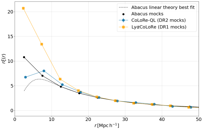
Figure 1: Comparison of the QSO auto-correlation function measured in the LyaCoLoRe mocks used in DR1 (yellow), the CoLoRe-QL mocks presented here (blue), and the quasar catalogs from the Abacus simulation (black) at $z=2.5$. The dashed black line is the best-fit linear theory to the Abacus mocks.

As shown in Figure 6 of [34], the clustering of quasars in the LyaCoLoRe mocks used to validate the analysis of eBOSS DR16 and in DESI DR1 did not reproduce well the clustering seen in the quasar catalogs from the more realistic Abacus simulations [35], which we take as our benchmark for comparison. In order to improve this, the CoLoRe-QL mocks use a different biasing model than the exponential one used in the DR1 mocks [32]. We use a linear biasing model, where the density of quasars is proportional to the (lognormal) density of matter, but modified such that quasars can only populate cells with a (lognormal) matter density threshold following:

$$1+\delta_{Q} \propto 1+b_{Q}\delta_{M} \text{for}\ \delta_{M}>t$$

$$1+\delta_{Q} =0 \text{for}\ \delta_{M}\leq t$$ (1)

where $t$ is the threshold and $\delta_{Q}$ and $\delta_{M}$ represent the quasar and matter overdensities, respectively. The values of the linear bias and of the threshold density were tuned to match the amplitude of quasar clustering on linear scales from a preliminary, blinded measurement of quasar clustering in DESI DR1. Both parameters vary as functions of redshift, and their precise configuration details are available in the corresponding configuration file In Figure 1, we compare the quasar clustering from LyaCoLoRe, CoLoRe-QL, and Abacus mocks. The results show that the CoLoRe-QL mocks are in better agreement with the Abacus mocks down to smaller scales.

II.2 Synthetic quasar spectra for DESI DR2

After generating the quasar positions and the skewers of Ly$\alpha$ transmission described in Section II.1, referred to here as the raw mocks, we use the desisim package to emulate the characteristics of the DESI DR2 Ly$\alpha$ quasar sample as closely as possible.

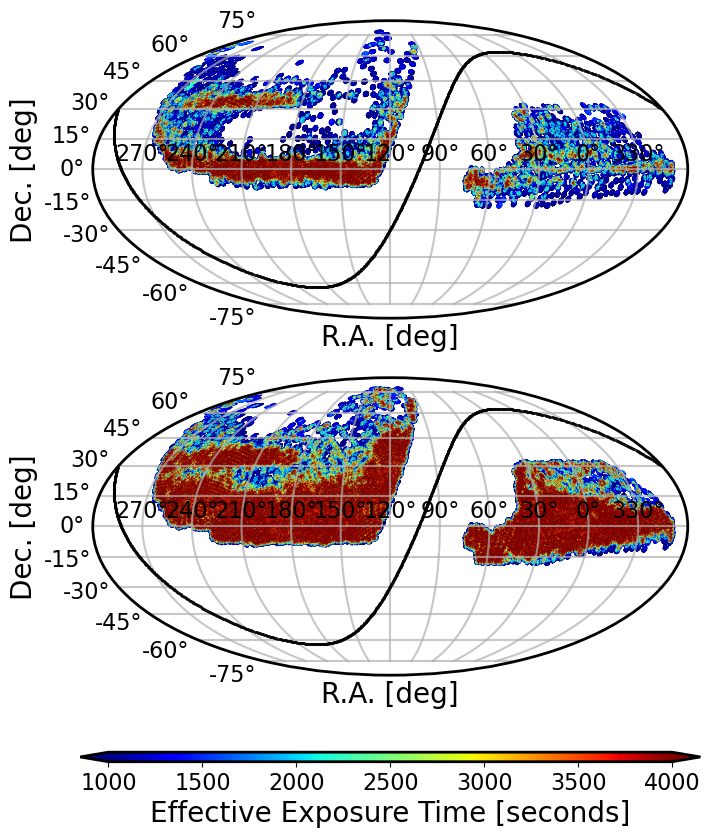
Figure 2: Comparison of the footprints in DESI DR1 (top) and DR2 (bottom). The colors show the effective exposure time.

The first step is to downsample the simulated quasar catalog to match the footprint and redshift distribution of quasars in DR2. Next, we randomly assign an $r$-band magnitude and number of exposures to each quasar following the observed distributions, as described in Section 2.2 of [28]. Figure 2 shows a comparison of the footprints in DR1 and DR2 of DESI. Since our mocks do not have gravitationally collapsed objects, we mimic the impact of non-linear peculiar velocities by adding random shifts to the quasar redshifts, following a Gaussian distribution with a dispersion of $\sigma_{\rm FoG}=150~{\rm km~s^{-1}}$, which is the expected velocity dispersion for halos with $\sim 10^{12}h^{-1}\,M_{\odot}$ characteristic mass hosting quasars at $z>2.0$ [36].

The second step is to generate synthetic spectra for each of the simulated quasars. For this we use the script quickquasars, described in detail in [37]. The Ly$\alpha$ skewers with the transmitted flux fraction a shown in the top panel of Figure 3 are modified to include various astrophysical contaminants, such as High Column Density systems (HCDs), Broad Absorption Lines (BALs) and other transition lines (metals). These are then multiplied by random (unabsorbed) quasar spectra (quasar continua), which are generated following the SIMQSO package [38]. Finally, we use the specsim package [39] to add instrumental noise representative of DESI during nominal dark-time conditions . An example of a mock spectrum after adding instrumental noise is shown on the bottom panel of Figure 3. For further details on the synthetic spectra generation procedure, we refer the reader to Sections 2 and 3 of [37].

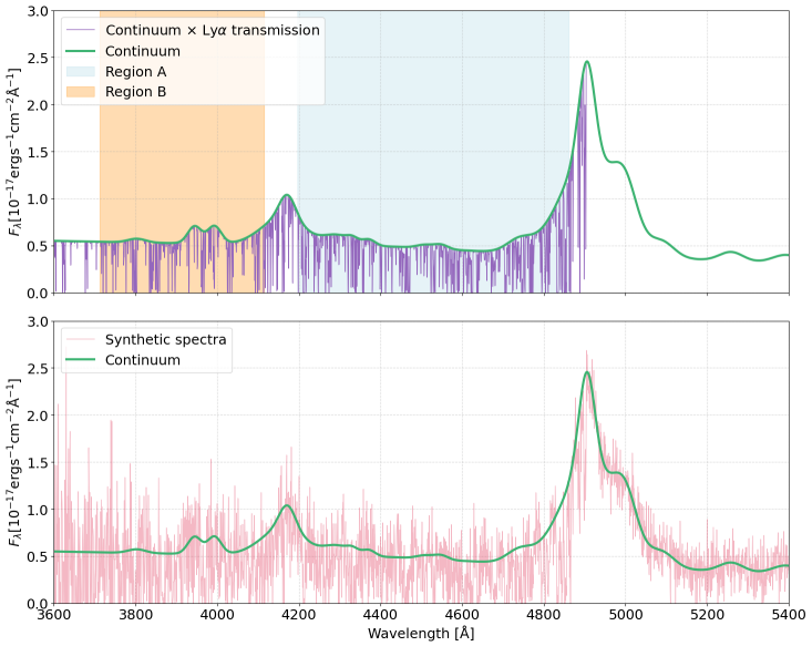
Figure 3: Simulated spectra from a CoLoRe-QL mock at $z=3.03$. Top panel: The green curve represents the quasar continuum as calculated by quickquasars, while the purple lines show the Ly$\alpha$ absorption, obtained by multiplying the transmission flux fraction with the quasar continuum. The shaded regions, A (blue) and B (orange), highlight the different areas used for calculating the correlations. Bottom panel: The pink line illustrates the simulated flux after incorporating instrumental noise using specsim.

As discussed in [27], approximately 15% of the observed quasars in DR2 were originally targeted as Emission Line Galaxies (ELGs). These have a different redshift-magnitude distribution and only have one observation (Ly$\alpha$ quasars in DESI can have up to four observations). These quasars were not included in the DR1 mocks presented in [28]. In the DR2 mocks we have included these extra quasars, using similar recipes to the ones used to generate the quasar targets, and ignoring the fact that quasars targeted as ELGs could have different spectral properties than those targeted as quasars.

After generating the mock spectra, we create in post-process a quasar catalog where we additionally include a random error on the reported redshift that emulates the statistical uncertainties from quasar redshift estimation algorithms such as redrock [40, 41] or QuasarNET [42]. We add these errors following a Gaussian distribution with a dispersion of $\sigma_{z}=400~{\rm km~s^{-1}}$, based on the measurements from [43]. Redshift errors cause a contamination in the measured correlations that was first identified in [34], and their impact on the measurement of BAO was partly discussed in section 4.4 of the paper describing the validation of the DR1 Ly$\alpha$ analysis [28]. In this work, we include these redshift errors in the baseline configuration of the analysis. We discuss the results and propose an strategy to mitigate their effect in Section V.

III Methodology

This work aims to validate the BAO analysis of Ly$\alpha$ forest measurements from DESI DR2 using the mocks described in Section II. In this section, we outline the entire process from simulated spectra to BAO measurements. We describe our method for extracting Ly$\alpha$ forest catalogs in Section III.1, computing the Ly$\alpha$ flux overdensity field in Section III.2, estimating Ly$\alpha$ correlation functions in Section III.3, and modeling these correlations in Section III.4. Finally, we explain how the BAO parameters are extracted by fitting the model to the measured correlation functions in Section III.5. The first three steps are implemented using the publicly available picca,while the modeling and fitting are conducted with the Vega package. The methodology followed here is similar to the one used in the analysis of the DR1 mocks [28], but we have introduced a couple of changes that we highlight below.

III.1 The Ly$\alpha$ forest catalog

In this section, we summarize the procedure for deriving a Ly$\alpha$ forest catalog from simulated quasar spectra. We begin by applying two observed-frame wavelength cuts to the spectra. The lower limit, $\lambda_{\mathrm{min}}=3600\,\mathrm{\AA }$, corresponds to the minimum wavelength detected by the blue arm of the DESI spectrographs, while the upper limit, $\lambda_{\mathrm{max}}=5772\,\mathrm{\AA }$, marks the midpoint of the overlap region between the blue and red arms of the spectrographs.

We continue by extracting the Ly$\alpha$ forest from two distinct regions of the spectra. As shown in Figure 3, region A spans the rest-frame wavelength range $\lambda_{\mathrm{RF}}[\mathrm{\AA }]\in[1040,1205]$, which is delimited by Ly$\alpha$ and Ly$\beta$ lines, while region B covers $\lambda_{\mathrm{RF}}[\mathrm{\AA }]\in[920,1020]$. The rationale for using two regions is that region A contains absorption exclusively from the first line of the Lyman series, Ly$\alpha$, while region B also includes higher-order absorption lines such as Ly$\beta$ and Ly$\gamma$. Although both regions are affected by absorption from other transition lines (metals), we assume all absorption is due to Ly$\alpha$ when measuring the correlation functions (Section III.3) and later model their impact on these (Section III.4).

We use Ly$\alpha$ pixels to refer to those pixels in the rest-frame wavelength regions defined above, and we refer to the collection of all Ly$\alpha$ pixels within a quasar spectrum as a forest. The combination of the observed- and rest-frame selection criteria constrain the redshift range of quasars contributing Ly$\alpha$ pixels in the region A to $z\in[2.1,4.4]$ and in the region B to $z\in[2.6,5.1]$. The number of quasars contributing to regions A and B in the mocks is approximately 800 000 and 360 000, respectively.

Before extracting the Ly$\alpha$ overdensity field, we apply corrections to mitigate the impact of two astrophysical contaminants: damped Ly$\alpha$ systems (DLAs) and broad absorption line quasars (BALs). We first identify pixels associated with DLAs detected at a signal-to-noise ratio greater than 2 and with column densities $N_{\rm HI}>10^{\mathrm{20.3}}{\rm cm}^{-\mathrm{2}}$. The DLA detection algorithm achieves a completeness of 75% for such systems [44]. To replicate the impact of DLAs in observations, we randomly mask the same fraction of DLAs that satisfy these criteria in the mocks. Specifically, we mask all DLA pixels where the transmitted flux decreases by 20% or more and correct the transmitted flux of the remaining DLA pixels using a Voigt profile [45] (see also Appendix B). For the validation of the DR1 measurement using mocks, we assumed 100% completeness for the DLA finder, thereby masking all DLAs in the mocks [28].

We mask the expected locations of all potential BAL features, regardless of whether the absorption is apparent [46]. These features include Ly$\alpha$, N IV, C III, Si IV, and P V in region A, and O VI, O I, Ly$\beta$, Ly$\gamma$, N III, and Ly$\delta$ in region B. Finally, we discard forests with fewer than 150 pixels, which is a threshold required by the continuum fitting procedure (see next section).

III.2 The flux transmission field

In this section, we provide a brief overview of our method for measuring the Ly$\alpha$ flux transmission field. We follow the same approach used for analyzing DR1 measurements; see [20, 28], for more details.

We begin by calculating the Ly$\alpha$ flux overdensity field, given by

$$\delta_{q}=\frac{f_{q}(\lambda)}{\bar{F}(z)C_{q}(\lambda)}-1,$$ (2)

where $f_{q}$ is the observed flux density for a quasar $q$, $C_{q}$ is the unabsorbed flux density (also referred to as the quasar continuum), $\bar{F}$ is the mean transmission of the intergalactic medium (IGM) at the absorber redshift $z=\lambda/\lambda_{\alpha}-1$, and $\lambda_{\alpha}$ is the rest-frame wavelength of Ly$\alpha$.

Measuring the flux overdensity field requires estimating the product $\bar{F}(z)C_{q}(\lambda)$ for each quasar. This step is known as continuum fitting, which is described in detail in [47, 48]. Here, we provide a brief overview of the process, noting that we perform it separately for regions A and B. First, we approximate the product $\bar{F}(z)C_{q}(\lambda)$ for each quasar as the product of $\bar{C}$, which is the same for all quasars, and a quasar-specific first-degree polynomial in $\Lambda=\log\lambda$,

$$E_{q}^{X}=\bar{C}^{X}(\lambda_{\mathrm{RF}})\left(a_{q}^{X}+b_{q}^{X}\frac{\Lambda-\Lambda_{\mathrm{min}}}{\Lambda_{\mathrm{max}}-\Lambda_{\mathrm{min}}}\right),$$ (3)

where $X$ refers to regions A and B, $\lambda_{\mathrm{RF}}=\lambda/(1+z_{q})$, and $\Lambda_{\mathrm{max}}$ and $\Lambda_{\mathrm{min}}$ correspond to the maximum and minimum observed-frame wavelengths of the forest for the quasar $q$. We fit $a_{q}^{X}$ and $b_{q}^{X}$ by maximizing the likelihood function

$$\ln{\mathcal{L}}=-0.5\sum_{i}\left[\frac{f_{q}(\lambda_{i})-E_{q}^{X}(\lambda_{i})}{\sigma_{q}^{X}(\lambda_{i},a_{q}^{X},b_{q}^{X})}\right]^{2}-\sum_{i}\ln{\sigma^{X}_{q}\left(\lambda_{i},a_{q}^{X},b_{q}^{X}\right)},$$ (4)

where $(\sigma_{q}^{X})^{2}=\eta_{\rm pip}^{X}(\lambda)\sigma_{{\rm pip},\,q}^{2}(\lambda)+[\sigma^{X}_{\rm LSS}(\lambda)E_{q}^{X}(\lambda)]^{2}$ is the flux variance of each pixel, $\sigma_{{\rm pip},q}^{2}$ is the pipeline estimate for the flux variance, $\eta_{\rm pip}^{X}$ is a correction factor for inaccuracies in this estimate, and $\sigma^{X}_{\rm LSS}$ represents the intrinsic standard deviation of fluctuations in the Ly$\alpha$ forest. Continuum fitting is an iterative process that begins by assuming initial values for $\bar{C}^{X}$, $\eta_{\rm pip}^{X}$, and $\sigma^{X}_{\rm LSS}$. The coefficients $a_{q}^{X}$ and $b_{q}^{X}$ are then computed for each region of all quasars. Next, we estimate the Ly$\alpha$ flux overdensity field for all forests, calculate its variance, and adjust the values of $\eta_{\rm pip}^{X}$ and $\sigma^{X}_{\rm LSS}$. Finally, we measure $\bar{C}^{X}$ and repeat the whole process until convergence, which typically takes 5 steps.

As first discussed in [49, 50], when fitting the $a_{q}^{X}$ and $b_{q}^{X}$ coefficients for each quasar we are suppressing very long wavelength fluctuations in the Ly$\alpha$ forest, distorting the measured correlations. In order to make the modeling of the distortion easier, we follow [51] and we explicitly subtract the mean and first moment from each forest, using the same weights used in the measurement of the correlations (see Eq. 8).

III.3 Measuring the correlation functions

There are six possible correlations involving quasar positions and Ly$\alpha$ fluctuations in regions A and B. However, following recent Ly$\alpha$ BAO analyses [47, 20], we focus on those with the highest signal-to-noise ratio: the auto-correlation of Ly$\alpha$ fluctuations in region A, $\xi^{\mathrm{AA}}$; the cross-correlation of Ly$\alpha$ fluctuations between regions A and B, $\xi^{\mathrm{AB}}$; and the cross-correlation of quasar positions with Ly$\alpha$ fluctuations in regions A and B, denoted as $\xi^{\mathrm{QA}}$ and $\xi^{\mathrm{QB}}$, respectively. In this section, we briefly outline our methodology for measuring these correlations, which is the same as the one used in the DR1 analysis and its validation. See [52, 28] for further details.

We compute the correlation functions on a grid of separations, $r_{\parallel}$ and $r_{\perp}$, corresponding to distances along and across the line of sight, respectively. This requires assuming a fiducial cosmology to convert angular and redshift differences into comoving separations

$$r_{\parallel}=[D_{C}(z_{i})-D_{C}(z_{j})]~\mathrm{cos}\left(\frac{\theta_{ij}}{2}\right),$$ (5)

$$r_{\perp}=[D_{M}(z_{i})+D_{M}(z_{j})]~\mathrm{sin}\left(\frac{\theta_{ij}}{2}\right),$$ (6)

where $i$ and $j$ index pixel-pixel or pixel-quasar pairs, pixel redshifts are determined by assuming Ly$\alpha$ absorption as $z_{i}=\lambda/\lambda_{\alpha}-1$, $\theta_{ij}$ refers to the angular separation, and $D_{C}$ and $D_{M}$ denote the comoving and angular comoving distances, respectively, which are identical in a flat Universe. We use the best-fitting flat $\Lambda$CDM model from Planck 2015 results [53] as our fiducial cosmology, the same model used to generate the LyaCoLoRe mocks.

The algorithms to compute the auto and the cross-correlations can be expressed in the following compact form

$$\hat{\xi}_{M}^{XY}=\frac{\sum_{i,j\in M}w_{i}^{X}w_{j}^{Y}\hat{\delta}_{i}^{X}\hat{\delta}_{j}^{Y}}{\sum_{i,j\in M}w_{i}^{X}w_{j}^{Y}},$$ (7)

where $X$ and $Y$ correspond to the auto- and cross-correlation cases defined at the beginning of this section, $M$ represents a two-dimensional bin with widths $(\Delta r,\Delta r)$, and $\delta^{\mathrm{Q}}=1$. The weight assigned to quasar $i$ is given by $w_{i}^{\mathrm{Q}}=\left[(1+z_{i})/(1+z_{\mathrm{Q}})\right]^{\gamma_{\mathrm{Q}}-1}$, where $z_{\mathrm{Q}}=2.25$ and $\gamma_{\mathrm{Q}}=1.44$ are derived from previous analyses [55]. The weights for Ly$\alpha$ fluctuations in regions A and B are

$$w_{i}^{X}=\frac{\left[(1+z_{i})/(1+z_{\rm fid})\right]^{\gamma_{\alpha}-1}}{\eta_{\rm pip}^{X}(\lambda)\sigma^{2}_{\mathrm{pip},q}(\lambda)[E_{q}^{X}(\lambda)]^{-2}+\eta_{\mathrm{LSS}}[\sigma^{X}_{\mathrm{LSS}}(\lambda)]^{2}},$$ (8)

where $\gamma_{\alpha}=2.9$ [56]. The term $\eta_{\mathrm{LSS}}=7.5$ enhances the contribution of the intrinsic Ly$\alpha$ forest variance relative to the pipeline noise, which improves the precision of the correlation function [48].

We measure the correlation functions using bins of $\Delta r=4\,h^{-1}\mathrm{Mpc}$ in both the radial and perpendicular separations. For the auto-correlations, we use 50 bins spanning separations from 0 to $200\,h^{-1}\mathrm{Mpc}$ in both directions. For the cross-correlations, we differentiate between pixels located in front of ($r_{\parallel}<0$) and behind ($r_{\parallel}>0$) quasars. With this distinction, we measure the cross-correlations using 50 bins for the perpendicular separation (0 to $200\,h^{-1}\mathrm{Mpc}$) and 100 bins for the parallel separation (-200 to $200\,h^{-1}\mathrm{Mpc}$).

We compute the covariance matrix associated with the correlations using the same approach as in previous DESI Ly$\alpha$ analyses [28]. First, we divide the mock survey footprint into HEALPix pixels [57] with $N_{\mathrm{side}}=16$, each covering approximately $3.7\times 3.7=13.4\,\mathrm{deg}^{2}$ of the sky. We then compute the correlation functions independently for each of the 1028 HEALPix pixels spanned by the DESI DR2 dataset. After that, we estimate the covariance matrix from these measurements as follows:

$$C_{MN}=\frac{1}{W_{M}W_{N}}\sum_{s}W_{M}^{s}W_{N}^{s}(\hat{\xi}_{M}^{s}\hat{\xi}_{N}^{s}-\hat{\xi}_{M}\hat{\xi}_{N}),$$ (9)

where $W^{XY,s}_{M}=\sum_{ij\in(M,s)}w_{i}^{X}w_{j}^{Y}$ represents the summed weight for a correlation in subsample $s$, $W^{s}=\{W^{\mathrm{AA},s},W^{\mathrm{AB},s},W^{\mathrm{QA},s},W^{\mathrm{QB},s}\}$ is a vector containing the summed weights for all correlations, $\hat{\xi}=\{\xi^{\mathrm{AA}},\xi^{\mathrm{AB}},\xi^{\mathrm{QA}},\xi^{\mathrm{QB}}\}$ refers to a vector containing the correlations, and $W_{M}=\sum_{s}W_{M}^{s}$ denotes the total weight.

The covariance matrix in our fiducial analysis has dimensions $15\,000\times 15\,000$, making its estimation inherently noisy due to the limited number of subsamples. To mitigate this noise, we smooth the covariance matrix of each mock using the same procedure as in previous analyses [28]. This smoothing method is also applied when computing the covariance of the stack of multiple mocks.

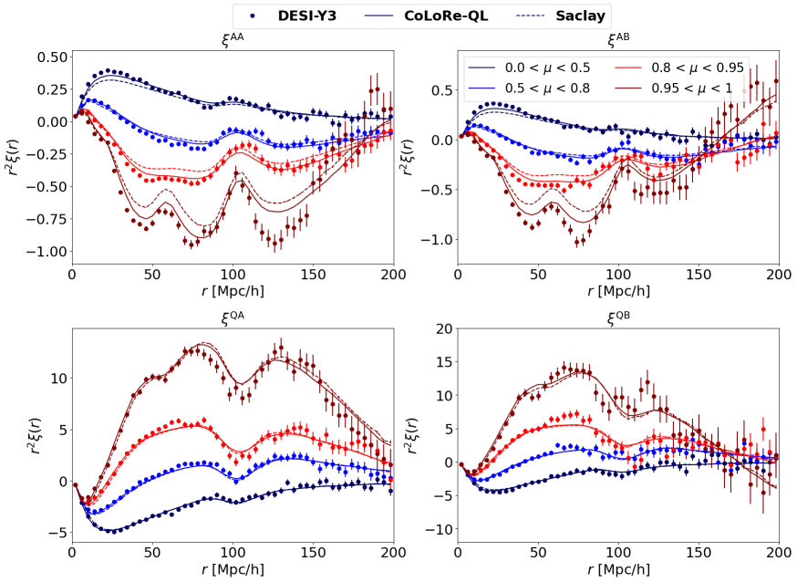
Figure 4: Comparison between DESI DR2 observational measurements and mock predictions. The panels, in clockwise order, display the following: the auto-correlation of the Ly$\alpha$ forest in region A, the auto-correlation of the Ly$\alpha$ forest in regions A and B, the cross-correlation of the Ly$\alpha$ forest in region B with quasar positions, and the cross-correlation of the Ly$\alpha$ forest in region A with quasar positions. Data points and error bars represent the observational measurements and their associated uncertainties, while the solid and dashed lines represent the results from the average of 300 CoLoRe-QL and 100 Saclay mocks, respectively. The colors of the lines indicate the average correlations in different wedges. Overall, the mocks show good agreement with the observational measurements; however, their accuracy diminishes for the line-of-sight wedge in the auto-correlations.

In Figure 4, we compare the four correlation functions derived from DESI DR2 observations (data points) with the averages of 300 CoLoRe-QL mocks (solid lines) and 100 Saclay mocks (dashed lines). The measurements are presented as a function of radial separation, $r=(r_{\parallel}^{2}+r_{\perp}^{2})^{1/2}$, and the wedges defined by $\mu=r^{-1}r_{\parallel}$. Overall, the mock measurements agree well with the observational data across the entire range of scales, supporting the use of these mocks for assessing the performance of the correlation model (see Section III.4) in estimating the BAO position. However, we can readily see minor discrepancies in the auto-correlations, particularly in the line-of-sight wedge of the Saclay mocks. These differences primarily stem from the imperfect modeling of DLAs, redshift errors, and metal contamination in the mocks. Differences in other wedges of the auto-correlations are largely attributable to inaccuracies in modeling Ly$\alpha$ biasing on nonlinear and quasi-linear scales.

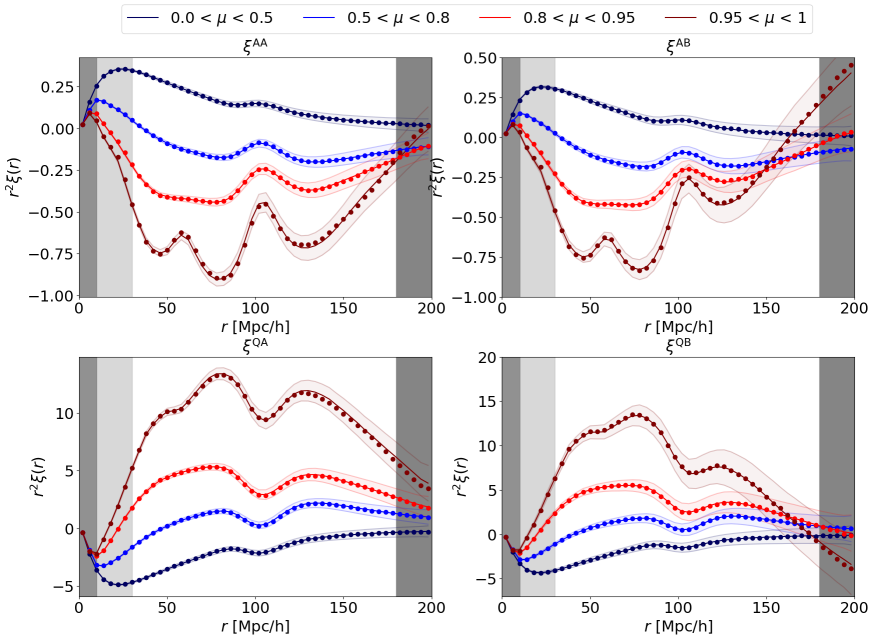
Figure 5: Best-fitting model to the average correlation of 300 CoLoRe-QL mocks. Dots represent the simulation measurements, lines correspond to the best-fitting model, and the shaded areas around the lines indicate the diagonal elements of the covariance matrix estimated from DESI DR2 measurements. The dark-shaded areas highlight the scales not used in this particular fit, while the light-shaded are show the scales that are not used in the main BAO analysis of DR2.

III.4 Modeling the correlation function

Our goal is to measure the BAO scale both along and across the line of sight. To this end, we use a model first introduced for the analysis of the Data Release 9 of BOSS [6, 4, 5], and progressively improved over the analysis of other data releases of BOSS [7, 58, 51, 55], eBOSS [59, 60, 47] and DESI [52, 28, 20]. In what follows, we progressively build this model and detail some differences compared to DESI DR1.

We begin with the isotropic linear matter power spectrum, $P_{\mathrm{fid}}$, computed evaluating CAMB [61] for the same fiducial cosmology used to convert angles and redshifts into comoving coordinates in the previous section. Next, we decompose $P_{\mathrm{fid}}$ into an oscillatory component, $P_{\mathrm{BAO}}$, which contains the BAO signal, and a smooth component, $P_{\mathrm{smooth}}$, using the algorithm described in [6]. To account for nonlinear effects, we apply an anisotropic Gaussian damping to the oscillatory component

$$P_{\mathrm{QL}}(k_{\parallel},k_{\perp},z)=P_{\mathrm{BAO}}(k,z)e^{-(k_{\parallel}^{2}\Sigma_{\parallel}^{2}+k_{\perp}^{2}\Sigma_{\perp}^{2})/2}+P_{\mathrm{smooth}}(k,z),$$ (10)

where $k=(k_{\parallel}^{2}+k_{\perp}^{2})^{1/2}$ is the wavevector, with $k_{\parallel}$ and $k_{\perp}$ as the parallel and perpendicular components, and where $\Sigma_{\parallel}$ and $\Sigma_{\perp}$ control the non-linear broadening of BAO along and perpendicular to the line of sight.

Building on the previous expression, we construct a model for the anisotropic power spectrum of the auto-correlations (X=Y=$\alpha$) and the cross-correlations (X=Q, Y=$\alpha$) as follows:

$$P_{XY}=b_{X}(z)(1+\beta_{X}\mu_{k}^{2})b_{Y}(z)(1+\beta_{Y}\mu_{k}^{2})$$ (11)

$$G(k,\mu_{k})F_{\mathrm{NL}}^{XY}(k,\mu_{k})F_{\mathrm{SM}}(k,\mu_{k})P_{\mathrm{QL}}(k,\mu_{k},z),$$

where $\mu_{k}=k^{-1}k_{\parallel}$ denotes the cosine of the angle between the wavevector and the line of sight. The factor $b(1+\beta\mu_{k}^{2})$ accounts for the impact of linear bias and redshift-space distortions [62] and the redshift evolution of the Ly$\alpha$ and quasar bias is modeled as $b_{X}(z)=b_{X}(z_{\mathrm{eff}})\left[(1+z)/(1+z_{\mathrm{eff}})\right]^{\gamma_{X}}$. We derive the value of $\beta_{\mathrm{Q}}$ from the linear bias assuming the fiducial cosmology: $\beta_{\mathrm{Q}}=b_{\mathrm{Q}}^{-1}f(z_{\mathrm{eff}})$, where $f$ is the linear growth rate of velocity perturbations. Note that we describe the correlations involving both Ly$\alpha$ regions (A and B) with the same model.

The term $G(k,\mu_{k})=\mathrm{sinc}(k_{\parallel}\Delta r/2)\mathrm{sinc}(k_{\perp}\Delta r/2)$ accounts for the binning of the correlation function on a grid [51]. Following [28], in order to account for the finite resolution of the mocks we multiply the power spectra by a Gaussian anisotropic smoothing factor: $F_{\mathrm{SM}}=\exp{-[(k_{\parallel}\sigma_{\parallel})^{2}+(k_{\perp}\sigma_{\perp})^{2}]/2}$. $F_{\mathrm{NL}}$ accounts for non-linear corrections that are limited to relatively small scales. When modeling the cross-correlations, we include the terms $F_{\mathrm{NL}}^{\mathrm{Q}\alpha}=\exp\left[-(k_{\parallel}\sigma_{v})^{2}/2\right]$ to model the combined impact of quasar redshift errors and non-linear peculiar velocities. When modeling the auto-correlation from observational data, we introduce a term $F_{\mathrm{NL}}^{\alpha\alpha}$ to account for the effects of nonlinear growth, peculiar motions, and thermal broadening on the auto-spectrum, using a model from [63]. These effects are not included in the mocks, and therefore we ignore them when modeling the correlations measured from mocks.

Finally, we account for potential systematic errors in quasar redshift measurements by introducing a systematic shift ($\Delta r_{\parallel}$) in the line-of-sight separation between quasars and Ly$\alpha$ absorption [64, 43].

Next, we transform the anisotropic power spectra from Fourier to configuration space. This is done by first performing a multipole decomposition of the anisotropic power spectrum up to $\ell=6$, followed by a Hankel transform using the FFTLog algorithm [65] implemented in the mcfit package to obtain the correlation function multipoles. From these multipoles, we then compute the two-dimensional correlation function $\xi^{XY}_{M}$ on a grid with spacing $\Delta r=2\,h^{-1}\mathrm{Mpc}$. We verified that including higher-order multipoles ($\ell>6$) does not affect BAO measurements. Additionally, we use a finer grid than the one used for measuring the correlation functions, $\Delta r=4\,h^{-1}\mathrm{Mpc}$, to improve the precision of the model.

Next, we model the impact of astrophysical contaminants and systematics on the correlation functions. Given the range of separations considered in our analysis, we account for the influence of four metal absorption lines: SiII(1190), SiII(1193), SiIII(1207), and SiII(1260). This requires computing correlation function models for all Ly$\alpha$-metal, QSO-metal, and metal-metal correlations using nearly the same framework as for Ly$\alpha$-only correlations. Each metal line is characterized by parameters $b_{i}$ and $\beta_{i}$, where $i$ runs over the four metal lines. Following [52], we fix $\beta_{i}=0.5$ and allow $b_{i}$ to vary freely in the fits. This leads to the following expressions for the auto- and cross-correlations:

$$\tilde{\xi}^{\alpha\alpha}=\xi^{\alpha\alpha}+\sum_{i}\xi^{\alpha i}+\sum_{ij}\xi^{ij}+\xi^{\mathrm{inst}},$$ (12)

$$\tilde{\xi}^{\mathrm{Q}\alpha}=\xi^{\mathrm{Q}\alpha}+\sum_{i}\xi^{\mathrm{Q}i}+\xi^{\mathrm{TP}},$$ (13)

where $\xi^{\mathrm{inst}}$ and $\xi^{\mathrm{TP}}$ represent the contributions from DESI instrumental systematics and quasar radiation effects, respectively. However, since these effects are not included in the mocks, we chose not to account for them in the analysis (see also [28]).

For the auto- and cross-correlations with metals, we account for the misestimation of pixel redshifts due to the assumption that all absorption originates from Ly$\alpha$. Specifically, we compute the redshift of each Ly$\alpha$ pixel as $z=\lambda/\lambda_{\alpha}-1$, whereas some absorptions are actually caused by metal lines, meaning their true redshifts should be $z=\lambda/\lambda_{\mathrm{metal}}-1$. As a result, these pixels are assigned to incorrect bins in the correlation function [66, 51]. We model this contamination with the same method used in the DR1 analysis [20], with a minor modification discussed in the companion paper [27].

As discussed in Section III.1, we mask pixels that are most contaminated by DLAs. However, as discussed in [44], we only mask DLAs detected in spectra with relatively high signal-to-noise (SNR$>$2), where the efficiency of the DLA finders is high, finding roughly 75% of the DLA systems

. Additionally, there are intermediate column-density systems not identified by the DLA-finding algorithm that contribute to contamination. Following [50, 67], we account for the impact of these contaminants by adding a scale-dependence to the bias and redshift-space distortion parameters of Ly$\alpha$ fluctuations to include the contributions from both Ly$\alpha$ absorption and HCDs

$$\tilde{b}_{\alpha}=b_{\alpha}+b_{\mathrm{HCD}}F_{\mathrm{HCD}}(k_{\parallel}),$$ (14)

$$\tilde{b}_{\alpha}\tilde{\beta}_{\alpha}=b_{\alpha}\beta_{\alpha}+b_{\mathrm{HCD}}\beta_{\mathrm{HCD}}F_{\mathrm{HCD}}(k_{\parallel}),$$ (15)

where $b_{\mathrm{HCD}}$ and $\beta_{\mathrm{HCD}}$ represent the contributions from HCD systems, while $F_{\mathrm{HCD}}(k_{\parallel})=\exp(-L_{\mathrm{HCD}}\,k_{\parallel})$ depends on the column density distribution of the HCDs present in the data.

The continuum fitting process (see Section III.2) notably alters the shape of the measured correlation functions [49, 50]. We use the formalism introduced in [51], that multiplies the modeled correlations $\tilde{\xi}$ by a distortion matrix $D^{XY}$:

$$\hat{\xi}_{M}^{XY}=\sum_{N}D_{MN}^{XY}\xi_{N}^{XY},$$ (16)

The distortion matrix can be computed from the geometry of the dataset and the distribution of weights, and in the DR2 analysis we have implemented an improved computation that takes into account the redshift evolution of the signal (see [27] for a detailed explanation and a discussion on the impact of this change).

III.5 Fitting the correlation function

By measuring the position of the BAO feature along and across the line of sight, we can constrain the distance ratios $D_{M}/r_{d}$ and $D_{H}/r_{d}$, where $r_{d}$ is the sound horizon at recombination, and $D_{H}(z)=c/H(z)$. In order to isolate this information from the rest of the measured correlations, in BAO analyses it is common to introduce two BAO parameters ($\alpha_{\perp}$, $\alpha_{\parallel}$) that only shift the position of the peak, without affecting the smooth component of the model:

$$\xi^{XY}=\xi_{\mathrm{smooth}}^{XY}(r_{\parallel},r_{\perp})+\xi_{\mathrm{BAO}}^{XY}(\alpha_{\parallel}r_{\parallel},\alpha_{\perp}r_{\perp}),$$ (17)

where $\alpha_{\parallel}=[r^{-1}_{\mathrm{d}}D_{\mathrm{H}}(z)]/[r^{-1}_{\mathrm{d}}D_{\mathrm{H}}(z)]_{\mathrm{fid}}$ and $\alpha_{\perp}=[r^{-1}_{\mathrm{d}}D_{\mathrm{M}}(z)]/[r^{-1}_{\mathrm{d}}D_{\mathrm{M}}(z)]_{\mathrm{fid}}$ are defined with respect to the distances in the fiducial cosmology, denoted by “fid”.

Besides the two BAO parameters, our model to describe the correlations in mocks uses 12 nuisance parameters: 3 for Ly$\alpha$ and quasar biases and redshift-space distortions ($b_{\alpha}$, $\beta_{\alpha}$, and $b_{\mathrm{Q}}$), 3 for HCD systems ($b_{\mathrm{HCD}}$, $\beta_{\mathrm{HCD}}$, and $L_{\mathrm{HCD}}$), 4 for the linear biases of each metal line ($b_{\mathrm{SiII(1190)}}$, $b_{\mathrm{SiII(1193)}}$, $b_{\mathrm{SiIII(1207)}}$, and $b_{\mathrm{SiII(1260)}}$), and 2 for redshift errors ($\Delta r_{\parallel}$ and $\sigma_{v}$). We determine the best-fitting value of these parameters using iminuit. While the BAO parameters have flat, non-informative priors, we use informative priors for some of the less constrained nuisance parameters as shown in Appendix C.

In the results presented in the following section, we hold fixed the value of the smoothing parameters ($\sigma_{\parallel}$, $\sigma_{\perp}$ in the $F_{\rm SM}$ term of Eq. 11) that capture numerical artifacts in the simulations (these parameters are not included in the analysis of real data). In order to choose a value for these parameters, we do a preliminary fit of the mean of the 300 CoLoRe-QL and 100 Saclay mocks, including separations from 10 to $180~h^{-1}\,\mathrm{Mpc}$. We show the results from the fit in Figure 5. We find the values $\sigma_{\parallel}=2.0~h^{-1}\,\mathrm{Mpc}$ and $\sigma_{\perp}=1.7~h^{-1}\,\mathrm{Mpc}$ for the CoLoRe-QL mocks, and $\sigma_{\parallel}=2.2~h^{-1}\,\mathrm{Mpc}$ and $\sigma_{\perp}=2.2~h^{-1}\,\mathrm{Mpc}$ for the Saclay mocks. In the case of the CoLoRe-QL mocks, we also use this preliminary fit to infer the value of the non-linear BAO broadening parameters, finding $\Sigma_{\perp}=3.1~h^{-1}\,\mathrm{Mpc}$ and $\Sigma_{\parallel}=4.3~h^{-1}\,\mathrm{Mpc}$. These parameters are held fixed to these values in later analyses of the CoLoRe-QL mocks . While the broadening measured in the transverse direction is consistent with the theoretical expectation at this redshift ($\Sigma_{\perp}=3.26~h^{-1}\,\mathrm{Mpc}$), the line-of-sight broadening is a bit lower than the expected one ($\Sigma_{\parallel}=6.4~h^{-1}\,\mathrm{Mpc}$).

Even though the model is able to fit the correlations on mocks down to $r=10~h^{-1}\,\mathrm{Mpc}$, in the analysis of DESI DR2 observational data we are more conservative and use only separations in the range $r=30$ to $180~h^{-1}\,\mathrm{Mpc}$, corresponding to 1590 and 3180 bins for the auto- and cross-correlations (see [27] for a discussion on the range of separations used). This is the configuration used in the analyses presented in the following sections.

IV Results

In this section, we describe and discuss the results obtained from performing the BAO analysis on the mocks. The mocks are used to validate the BAO analysis in two ways: in Section IV.1 we use them to validate that our analysis pipeline is unbiased, and in Section IV.2 we use them to validate that the reported uncertainties on the BAO parameters are representative of the scatter between the measurement in different realizations.

IV.1 Investigating potential systematic biases in the BAO measurements

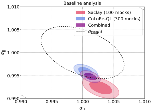
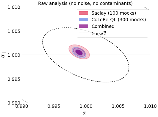
Figure 6: Top panel: best fit of the stacks using the and their combination (purple). The main difference with respect to DR1 is that we do continuum fitting after adding quasar redshift errors. As pointed out in [34], this introduces a spurious correlation that can result in a small bias on the BAO results. $\sigma_{\rm DESI/3}$ represents one third of the DR2 uncertainty. This corresponds to $0.0038$ for $\sigma_{\parallel}$ and $0.0045$ for $\sigma_{\perp}$. Bottom panel: BAO analysis on raw mocks without instrumental noise, contaminants, or continuum fitting. Both the Saclay and CoLoRe-QL mocks show no intrinsic biases, confirming that the observed shift is induced by the analysis.

In order to validate that our analysis pipeline produces unbiased BAO measurements, we combine the measurement from all our synthetic datasets to obtain correlation functions with very high signal-to-noise. Similarly to the other validation tests discussed in [27], our requirement was to recover the true BAO parameters ($\alpha_{\perp}$ = $\alpha_{\parallel}$ = 1) within a third of the statistical uncertainty from DESI DR2. Biases exceeding this threshold must be investigated, corrected, or incorporated into the systematic errors.

In the top panel of Figure 6 we show the BAO measurements from the combined (or stacked) correlations from 100 Saclay mocks (red) and 300 CoLoRe-QL mocks (blue), compared to the threshold of a third of the statistical uncertainty from DESI DR2 (dashed, black line). It is clear in the figure and in Table 1 that $\sigma_{\parallel}$ measurements are biased at high significance, with a bias near the threshold criterion we imposed, while $\sigma_{\perp}$ satisfies the criteria.

In order to distinguish between a bias in our analysis pipeline from a bias in our simulated boxes, in the bottom panel of Figure 6 we show a simplified BAO analysis where we measure the correlations directly from the raw mocks introduced in Section II.1. This analysis, detailed in Appendix A, does not require any continuum fitting and is not affected by instrumental noise or astrophysical contaminants. The fact that these results are unbiased relative to our threshold of $\sigma_{DESI}/3$, rule out intrinsic issues with the simulated boxes. Instead, as discussed in detail in V, we have identified that the bias in the baseline analysis (bottom panel) arises from the method used to incorporate redshift errors in the mocks catalogs.

	$\Delta\alpha_{||}$	$\Delta\alpha_{\bot}$	$\Delta\alpha_{iso}$	$\Delta\alpha_{AP}$
CoLoRe-QL (300)	$-0.0042\pm 0.0006$	$0.0005\pm 0.0008$	$-0.0020\pm 0.0004$	$0.0047\pm 0.0012$
Saclay (100)	$-0.0074\pm 0.0010$	$0.0031\pm 0.0012$	$-0.0027\pm 0.0005$	$0.0106\pm 0.0019$
Combined (400)	$-0.0052\pm 0.0005$	$0.0012\pm 0.0006$	$-0.0023\pm 0.0003$	$0.0065\pm 0.0010$

Table 1: Biases on the BAO parameters ($\alpha_{\parallel}$, $\alpha_{\perp}$) from the combined analyses of 300 CoLoRe-QL and 100 Saclay mocks, as well as their combination. The last two columns show the biases on the isotropic BAO parameter, defined here as $\alpha_{\rm iso}={\alpha_{\perp}^{9/20}\alpha_{\parallel}^{11/20}}$ and the anisotropic Alcock-Paczyński parameter $\phi=\alpha_{\perp}/\alpha_{\parallel}$. As discussed in Section V, these small biases can be attributed to the method used to add redshift errors in the mocks.

IV.2 Validating the BAO uncertainties

In this section we present the BAO results obtained by individually fitting each of the DESI DR2 mocks. In the top panel of Figure 7 we display the scatter of the best-fit BAO parameters across the 400 mocks (300 CoLoRe-QL and 100 Saclay). While there are no specific outliers, the measurements are not perfectly centered around the true values ($\alpha_{\perp}$ = $\alpha_{\parallel}$ = 1), particularly in the parallel direction, in agreement with the results from the stack of mocks (see Table 1).

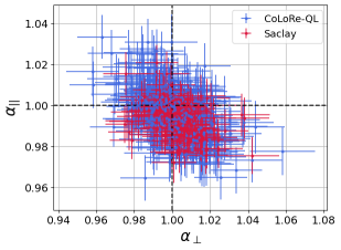
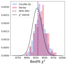
Figure 7: Top: Scatter plot of the best-fit BAO measurements obtained for each of the 100 Saclay mocks (red) and 300 CoLoRe-QL mocks (blue). Bottom: Distribution of $\chi^{2}$ values from the fits, compared to the expected distribution given the number of degrees of freedom (black). The dashed purple line represents the $\chi^{2}$ of the best fit to the data.

The bottom panel of Figure 7 shows the distribution of the best-fit $\chi^{2}$ values obtained from the fits of individual mocks. The black curve represents the expected distribution based on the degrees of freedom in the fit. The plot shows that the distribution of $\chi^{2}$ values is higher than expected, although the situation is significantly better than in the mocks used in the validation of DESI DR1 (see Figure 8 of [28]). In [28], Monte Carlo simulations starting from either the best-fit model or the stacked correlation function measurements demonstrate that this shift toward higher $\chi^{2}$ values arises from the model’s difficulty in fitting the correlation functions. This indicates that the issue is not related to the covariance matrix but rather to the limitations of the model, especially at small scales. Finally, the purple dashed line on this plot represents the $\chi^{2}$ of the data best-fit, which is reasonable given the distribution from the mocks.

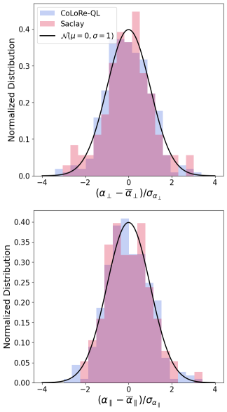
Figure 8: Histograms of BAO residuals, defined as $\Delta\alpha_{\parallel}/\sigma_{\alpha_{\parallel}}$ and $\Delta\alpha_{\perp}/\sigma_{\alpha_{\perp}}$, where the uncertainties are the Gaussian ones reported by iminuit in each individual fit. The results for the 100 Saclay mocks (red) and 300 CoLoRe-QL mocks (blue) are in good agreement with a Normal distribution (black lines), indicating that the posteriors are Gaussian and the uncertainties are well estimated.

We validate the method to estimate the BAO uncertainties in Figure 8, where we show the BAO residuals from the fit of each mock realization, defined as $\Delta\alpha_{\parallel}/\sigma_{\alpha_{\parallel}}$ and $\Delta\alpha_{\perp}/\sigma_{\alpha_{\perp}}$. The residual distributions closely follow a Normal distribution, represented by the black curve, presenting evidence that the BAO uncertainties are accurate and approximately Gaussian.

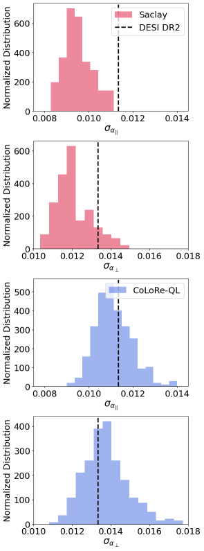
Figure 9: Distribution of uncertainties on $\alpha_{\parallel}$ and $\alpha_{\perp}$ for 100 Saclay mocks (top panel) and 300 CoLoRe-QL mocks (bottom panel). The black dashed line represents the uncertainties derived from the data, which align more closely with the CoLoRe-QL mocks, as the Saclay mocks lack non-linear broadening of the BAO peak.

Finally, in Figure 9, the uncertainties on BAO parameters of the mocks are shown alongside the statistical uncertainties from DESI data (vertical dashed line). The top panel shows the results for Saclay mocks in red, while the bottom panel shows CoLoRe-QL mocks in blue. As discussed in [28], non-linear broadening of the BAO peak modestly yet noticeably degrades the BAO measurements. Consequently, mocks that do not include this effect, such as the Saclay mocks, exhibit uncertainties that are smaller than those observed in the data. Specifically, the uncertainties in Saclay mocks are $10–20\%$ smaller than those in the DESI results. In contrast, the CoLoRe-QL mocks demonstrate better agreement with the data, as they include a certain degree of non-linear broadening, as discussed in Section II.1.2.

V Discussion

In Section IV.1 we presented the BAO measurements from the combined correlations measured in 300 CoLoRe-QL and 100 Saclay mocks. As shown in the top panel of Figure 6 and reported in Table 1, we detect a small but significant bias from the expected value ($\alpha_{\perp}=\alpha_{\parallel}=1$). In this section we demonstrate that this bias is caused by the method used to simulate redshift errors in the mocks (Section V.1), and propose a mitigation strategy to avoid most of the contamination when analyzing real data (Section V.2).

V.1 Analysis of mocks without redshift errors contamination

As discussed in Section II.2, once we have already simulated the quasar spectra we add a random shift to the redshifts in our quasar catalogs, creating a mismatch between the reported redshift of the simulated quasar and the positions of the emission lines in their spectra. This allows us to capture the impact of redshift errors in the real catalogs, without the need to run the redshift fitter Redrock [40] for hundreds of mocks.

The first clear impact of random quasar redshift errors in our analysis is that they smear the measured cross-correlations along the line of sight [64], similar to the impact of non-linear velocities (or fingers of God) in the clustering of quasars. As discussed in Section III.4, we model this impact by multiplying the power spectrum of the cross-correlation model by $F_{\mathrm{NL}}^{\mathrm{Q}\alpha}=\exp\left[-(k_{\parallel}\sigma_{v})^{2}/2\right]$.

Recently, [34] described a second, more subtle impact of redshift errors that cause spurious correlations not only in the cross-correlation with quasars, but also in the auto-correlation. As discussed in Section III.2, in order to compute the fluctuations in the Ly$\alpha$ forest we need to estimate the mean continua of all our quasars, as a function of rest-frame wavelength ($\bar{C}(\lambda_{\mathrm{RF}})$). However, the random shifts added to the redshifts of our mock catalogs are translated into mis-estimations of the rest-frame wavelengths, and this causes a smoothing of the features in the mean continuum, in particular of the emission lines present in the Ly$\alpha$ forest regions. This effect, coupled to the clustering of the background quasars, causes spurious correlations that could bias our results. These biases are discussed in more detail in [70].

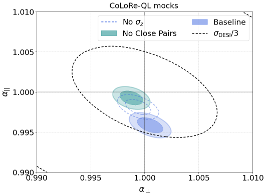
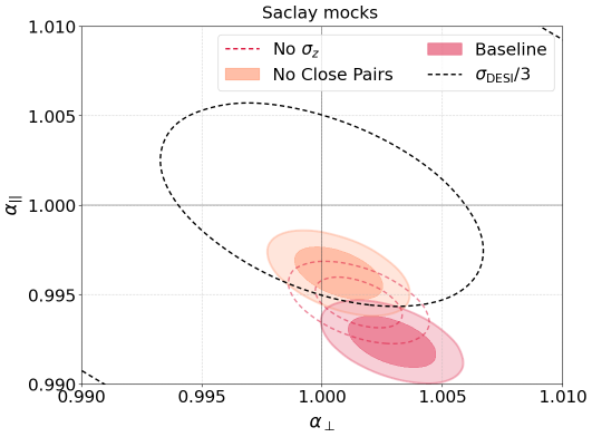
Figure 10: Comparison of ”No Close Pairs” and ”no $\sigma_{z}$” analyses with the baseline. Both approaches aim to mitigate contamination from redshift errors prior to continuum fitting, with ”No Close Pairs” excluding close quasar pairs (which are the most affected) and ”no $\sigma_{z}$” removing estimation redshift errors entirely before continuum fitting.

In order to test this hypothesis, in Figure 10 we present an alternative analysis (labeled no $\sigma_{z}$) where the random redshift errors are only added after the continuum fitting, so that they only impact the cross-correlation measurements by smoothing them along the line of sight with $F_{\mathrm{NL}}^{\alpha\mathrm{Q}}$. For both sets of mocks this alternative analysis is significantly less biased than our baseline configuration, bringing it below the threshold of one third of the DESI DR2 statistical uncertainty (dashed black line ellipses).

V.2 Mitigating the BAO scale bias by removing close pairs of quasars

Unfortunately, when analyzing real data we can not avoid having redshift errors affecting our continuum fitting. For this reason, in this section we propose an alternative analysis that should minimize its impact without losing a significant fraction of the data.

In a recent study, [70] presented a model that can describe the spurious correlations introduced by redshift errors. In that paper, the authors also show that most of the contamination in the cross-correlation comes from pixel-quasar pairs where the background quasar (whose spectrum contains the pixel) and the foreground quasar (whose position we are considering) are very close to each other. Similarly, they show that most of the contamination in the auto-correlation comes from pairs where one of the pixels is very close to the background quasar of the other pixel.

Motivated by this, in Figure 10 we also show an analysis (labeled No close pairs) where we do not include these problematic pairs, in particular those with angular separations smaller than 20 arcmin and velocity separations smaller than 4000 ${\rm km~s^{-1}}$. This analysis is significantly less biased than our baseline configuration, and more importantly, it can be done when analyzing real data. In [27] we present the results of this alternative analysis on real data, and show that it has a negligible impact on our main BAO results.

While both alternative analyses show effectively unbiased results when analyzing the stack of 300 CoLoRe-QL mocks (left panel), there seems to be a small bias when analyzing the stack of 100 Saclay mocks, even though significantly smaller than in the baseline analysis and no longer larger than the tolerance limit of $\sigma_{DESI}/3$. We have not been able to identify the cause for this residual bias in the analysis of the Saclay mocks.

Finally, it is important to note that the current method used to add random errors to the mocks could have exaggerated the contamination. One of the main sources of redshift errors is that some of the quasar emission lines used to estimate their redshifts (like C III, Si IV or C IV) can be affected by outflows or complex quasar physics. However, this should also affect the other high-ionization lines that are present in the Ly$\alpha$ region. This would reduce the amount of smoothing of the mean quasar continuum, the level of the spurious correlations and therefore the bias on the BAO measurements.

VI Summary

In this work, we use synthetic data to validate the analysis of Ly$\alpha$ BAO measurements from the second data release (DR2) of the Dark Energy Spectroscopic Instrument (DESI), presented in [27]. DR2 includes spectra from nearly 1.2 million quasars at redshift $z\geq 1.77$, nearly doubling the sample size of DESI DR1 [20]. As a result, DR2 achieves approximately a factor of two better statistical precision in Ly$\alpha$ forest BAO measurements compared to DR1, thereby necessitating a more rigorous validation of the cosmological inference pipeline.

The main differences between the validation of DR2 with respect to that of DR1 (presented in [28]) are the following. On the one hand, we have improved the mocks. We have increased the number of synthetic datasets used to validate the BAO analysis from 50 to 100 Saclay mocks [31] and from 100 to 300 LyaCoLoRe mocks [30]. We have presented the CoLoRe-QL mocks, an improved version of the LyaCoLoRe mocks used in DR1 that include the non-linear broadening of the BAO peak. On the other hand, we have improved the analysis to better mimic the analysis of real data. Instead of masking all the DLAs in the spectra (as done in the validation of DR1), we only mask DLAs in high signal-to-noise spectra (SNR$>$2), and only for a randomly-selected subset of 75% to emulate the completeness of the DLA catalog used in DR2 (see the discussion in Appendix B).

Using these mocks, we validated that the reported uncertainties on the BAO parameters are consistent with the scatter between the different realizations. Using the average measurement of correlations from all mocks, we have identified a small, but statistically significant bias in the line-of-sight BAO parameter. This bias is close to a third of the statistical uncertainty in DR2, the threshold that we had set to consider the analysis validated. We have shown that most of this bias is related to the redshift errors in the quasar catalog, a contamination first discussed in [34]. Following [70], we have presented an analysis that discards a small fraction of the data that is most contaminated, and we have shown that the residual bias is significantly smaller than our statistical uncertainty.

In the near future, we will present a cosmological analysis using the full shape information contained in the Ly$\alpha$ correlations, not limited to the position of the BAO peak [71, 72, 73]. In order to validate these analyses, it will be important to count on improved Ly$\alpha$ mocks that simulate the non-linear growth of structure, using perturbation theory models or similar. It will also be important to improve the method to add redshift errors to the simulated catalogs. In order to do this, it will be useful to have a dedicated study of the relative redshifts of the different emission lines in the quasar spectra.

VII Data Availability

The data used in this analysis will be made public along the Data Release 2 (details in https://data.desi.lbl.gov/doc/releases/). The data points corresponding to the figures from this paper will be available in a Zenodo repository.

Appendix A Analyses on raw mocks

We refer to a BAO analysis procedure applied on the raw mocks, described in Section II.1, without astrophysical contaminants, instrumental noise, or quasar continuum templates added as the raw analysis. This analysis allows us to verify that we are able to recover the position of the BAO peak specified by the input cosmology and discard an intrinsic bias on the raw mocks.

In this analysis, we do not have to perform the astrophysical contaminants masking or the continuum fitting procedures described in Sections III.1 and III.2, respectively, as they are not present in raw mocks. In other words, we compute the delta field from the transmitted flux fraction boxes directly by:

$$\delta_{q}(\lambda)=\frac{F(\lambda)}{\overline{F}(z)}-1.$$ (18)

The correlation functions are computed in the same way as in the standard analysis, described in Section III.3. However, in this case we do not smooth the covariance matrix since it is already positive definite given the high SNR of the raw analysis. Moreover, smoothing this covariance produces a non-positive definite matrix which induces a bias on the cross-correlation measurement on both Saclay and CoLoRe-QL mocks.

In the case of the model, described in Section III.4, we do not apply a distortion matrix or exclude astrophysical contaminants as these effects do not included in the raw analysis. Furthermore, we perform additional fits for the auto- and cross-correlations individually. We free the BAO parameters ($\alpha_{\parallel}$ and $\alpha_{\perp}$), the smoothing parameters ($\sigma_{\parallel}$ and $\sigma_{\perp}$), and Ly$\alpha$ linear bias and RSD parameters ($b_{\mathrm{Ly\alpha}}$ and $\beta_{\mathrm{Ly\alpha}}$). For the cross-correlation fit, we additionally fix the quasar bias ($b_{q}$) value to each type of mocks truth value ($b_{q}=3.123$ for CoLoRe-QL and $b_{q}=3.3$ for Saclay).

Figure 11 shows the results for CoLoRe-QL mocks (left panel) and Saclay mocks (right panel). The combined fit results for $\alpha_{||},\alpha_{\bot}$ are:

$$\alpha_{||}^{\mathrm{QL}}=1.0004\pm 0.0005,\qquad\alpha_{\bot}^{\mathrm{QL}}=0.9990\pm 0.0004,$$ (19)

and

$$\alpha_{||}^{\mathrm{Saclay}}=1.0009\pm 0.0006,\qquad\alpha_{\bot}^{\mathrm{Saclay}}=0.9992\pm 0.0007,$$ (20)

for CoLoRe-QL and Saclay mocks, respectively. All the results presented in Figure 11 are within a third of the statistical uncertainty from DESI DR2 threshold and close to the $\alpha_{||}=\alpha_{\bot}=1$ target value, confirming that the raw mocks are suitable to be used in the analysis validation presented in this work.

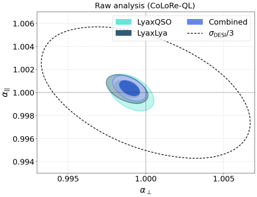
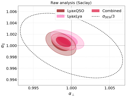
Figure 11: Top panel: Fit results for the auto-correlation alone, cross-correlation alone, and combined fit for CoLoRe-QL raw mocks. In the raw analysis there is no noise, no contaminants and no continuum fitting. Bottom panel: Same fits for Saclay raw mocks. All fits are compatible and unbiased.

Appendix B Impact of DLA masking

Damped Lyman-$\alpha$ absorbers (DLAs) are found and masked in the BAO analysis to optimize the statistical precision of the measurement, and any residual DLA contamination is accounted for via free parameters in the model fit. In this section, we use mocks to study the impact on BAO results when changing the DLA-finding algorithm and to find the optimal DLA catalog configuration for the DR2 BAO analysis on real data.

The Ly$\alpha$ BAO analysis from DESI DR1 [20] masked those DLAs that were found by both a Gaussian Process (GP) finder [74] and a convolutional neural network (CNN) finder [75]. Tests on one mock found the combination to produce unbiased BAO results compared to a catalog of all input DLAs [28]. In preparation for DR2 analysis, several improvements have been made to the GP and CNN finders, and an additional finder (referred to as the template, or TMP, finder) has been developed that fits each spectrum with a template for quasars and one or more DLA models [44].

To test the performance of these finders for the DR2 BAO analysis, we ran all three finders on one realization of the LyaCoLoRe mocks. After each DLA finder was run on the mock data, several quality cuts were made to the raw output catalogs. In a first series of analyses, all three finders were reduced to only include DLAs found in spectra for which the mean signal-to-noise measured on the red-side of the Ly$\alpha$ forest was $SNR>3$. Furthermore, only DLAs with high column density, $\log{\big{(}\frac{N_{\mathrm{HI}}}{cm^{-2}}\big{)}}>20.3$ for the $N_{\mathrm{HI}}$ calculated by each algorithm were kept. We included additional quality cuts, for the CNN confidence parameter CONF$>0.5$; for the GP probability parameter P_DLA$>0.9$; and for the TMP enforcement of DLAFLAG=0 (see [75, 74, 44] for further details on these parameters). The performance of the different algorithms, in terms of purity and completeness of their DLA catalogs, is discussed in the companion paper [44], and we refer the interested reader to that publication for more detail. Here we complement this study by looking at the impact on the BAO parameters when using different DLA finders.

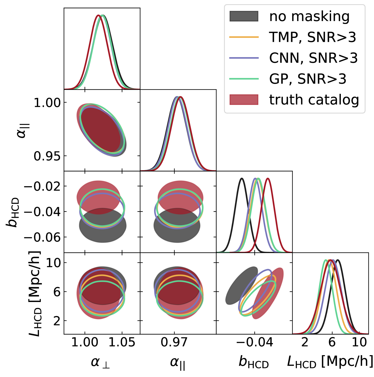
Figure 12: Contours for HCD parameters and BAO parameters under different DLA masking schemes. Only 95% confidence levels are shown. The results from the three DLA finders are shown in open contours to facilitate visualization, while the two extremes (no masking and truth catalog) are shaded. For $b_{\mathrm{HCD}}$, the finder-based analyses produce values lying between the two extremes as expected, and the $L_{\mathrm{HCD}}$ varies depending on the typical length scale masked. However, the BAO parameters (upper left) are stable to variations. The BAO parameters are in mild tension with the true input cosmology values because this is an analysis on only a single mock; the stack of mocks is unbiased as discussed in Section IV.1.

We ran different end-to-end BAO analyses on this particular LyaCoLoRe mock, but using different catalogs to mask DLAs, including an analysis without masking any DLA (labeled no masking) and an analysis that masked all the DLAs added to the mocks (labeled truth catalog). Figure 12 shows that the BAO parameters are very robust to the DLA catalog used, and the small differences can be explained by statistical fluctuations. However, each analysis has a different amount of residual contamination from DLAs that were not identified, and this translates into different values for the nuisance parameters describing the contamination by High Column Density systems (HCDs): $L_{\mathrm{HCD}}$, $\beta_{\mathrm{HCD}}$, and $b_{\mathrm{HCD}}$, presented in Section III.4. As expected, $b_{\mathrm{HCD}}$ varies between a large negative value for the no masking case, where a large contribution to the bias due to DLAs must be taken into account in the model, to a small negative value when all DLAs are removed and only small HCD contributions remains (truth catalog masking). The three DLA finders result in very similar values for $b_{\mathrm{HCD}}$ and all lie between the two extremes, having found most but not all DLAs in the fiducial catalog. $L_{\mathrm{HCD}}$, the typical length scale of DLA systems that appear in the data, is large when none are masked (because even large DLAs remain in the spectra) and decreases with any form of masking, because only smaller systems remain. The model succeeds in capturing the correlation function variations through the HCD parameters such that the choice of DLA masking does not bias the BAO parameters, as evidenced by the stability in $\alpha_{\parallel}$ and $\alpha_{\perp}$ parameters.

In order to decide on the optimal method to mask DLAs in the DR2 analysis, [44] studied possible ways to combine the catalogs constructed by the different DLA finders. Combined catalogs containing DLAs detected by at least two finders, when limited to spectra with $SNR>2$, resulted in similar performances in terms of completeness and purity of the catalogs, both around 75%. The recommendation from [44], that was adopted in the Ly$\alpha$ BAO measurement from DR2 of [27], was to mask DLAs that were identified by the GP finder and one of the other two finders , a combination that we label as GP+.

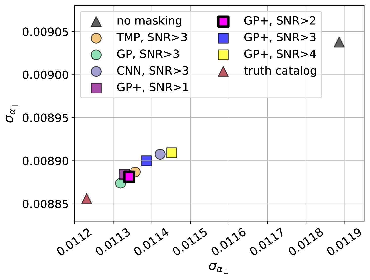
Figure 13: Forecasted uncertainties on $\alpha_{\parallel}$ and $\alpha_{\perp}$ for the one-finder (circles) and two-finder (squares) DLA catalogs compared to the case of no masking and masking all objects in the truth catalog (triangles). The final choice for data analysis is the GP+, SNR$>2$ catalog (pink square with bold borders), which has an optimal completeness-purity tradeoff in addition to performing with high precision, as shown here.

After the decision was made to use the GP+ catalog, we revisited the impact of different SNR cuts. Masking DLAs detected in lower SNR spectra would trade a lower purity of the sample for a higher completeness. In Figure 13 we compare the forecasted BAO uncertainties for different DLA masking strategies, in particular when varying the SNR threshold in the GP+ catalog. However, as the different finders mask different Ly$\alpha$ data, there is some natural sample variation in both the signal and the uncertainty of the resulting BAO parameters. This makes it challenging to directly compare the BAO uncertainties to make the optimal choice. To more robustly quantify the performance of each masking catalogue, we make a BAO forecast using vega. The forecast works by creating a vector that represents the correlation function but is purely equal to the (noiseless) best-fit model for that analysis. Using the covariance matrix of the mock data in combination with that vector, the BAO fit is performed, obtaining BAO uncertainties that are not affected by statistical fluctuations.

Figure 13 shows that the error on $\alpha_{\parallel}$ and $\alpha_{\perp}$ is highest when no DLAs are masked, and moves lower for the various finders, approaching the truth catalog case with smallest errorbars. Although GP on its own results in the smallest errors of the single-finder cases (circles), as previously stated, we deemed it more robust to require detection in at least one of the other finders. Of the SNR cuts tested for the GP+ catalog, the SNR$>2$ and SNR$>1$ versions perform best, so we choose SNR$>2$ for its higher purity for the BAO DR2 data analysis.

Given the trend to lower $\sigma_{\alpha_{\perp}}$ and $\sigma_{\alpha_{\parallel}}$ for increasing numbers of masked DLAs, it is interesting to question whether masking increasingly smaller DLAs would continue to reduce the error bars. Given that masking also removes Ly$\alpha$ signal, however, there must be a point at which the gains in precision due to removal of these contaminants are outweighed by the loss in signal. We explored this idea by masking not only all the DLAs added to the mocks, but also all the HCD systems with increasingly lower column density. By running vega forecasts, we find that the uncertainties continue to decrease until a threshold of $\sim\log{(N_{\mathrm{HI}})}>19$. However, beyond this, continuing to mask systems with even lower column density causes the uncertainties to increase again due to excess loss in Ly$\alpha$ signal. This investigation is not relevant to the DESI DR2 analysis, as the DLA finders are not expected to perform well at such low column densities; however, it demonstrates that with future improved algorithms, the analysis could benefit from masking lower column density systems.

Appendix C Details on the nuisance parameters

As discussed in Sections III.5 and IV, we perform various types of analyses on the mocks presented throughout this work. Table 2 provides a description of the free parameters used to model the correlation functions from our mocks in the range $30<r<180\ h^{-1}\mathrm{Mpc}$, with the corresponding priors listed in the second column.

The last two rows of this table specify the priors used for the finite-grid Gaussian smoothing parameters ($\sigma_{\parallel},\sigma_{\perp}$), and the non-linear BAO peak broadening parameters ($\Sigma_{\parallel},\Sigma_{\perp}$). These priors were applied exclusively in a fit on the high-precision BAO measurements described in Section IV.1 over $10<r<180~h^{-1}\,\mathrm{Mpc}$ to determine these parameters values. For all other analyses, these parameters remain fixed at $\sigma_{\parallel}=2.0~h^{-1}\,\mathrm{Mpc}$, $\sigma_{\perp}=1.7~h^{-1}\,\mathrm{Mpc}$, $\Sigma_{\parallel}=4.3\ h^{-1}\mathrm{Mpc}$, and $\Sigma_{\perp}=3.1\ h^{-1}\mathrm{Mpc}$ for CoLoRe-QL mocks, while for Saclay mocks, they are fixed at $\sigma_{\parallel}=\sigma_{\perp}=2.2~h^{-1}\,\mathrm{Mpc}$ and $\Sigma_{\parallel}=\Sigma_{\perp}=0$.

For the raw analyses presented in Appendix A, we only allow the BAO scale parameters ($\alpha_{\parallel},\alpha_{\perp}$), the Ly$\alpha$ linear bias and RSD parameter ($b_{\alpha},\beta_{\alpha}$), the quasar linear bias ($b_{\rm q}$), the finite-grid Gaussian smoothing parameters ($\sigma_{\parallel},\sigma_{\perp}$), and the non-linear BAO peak broadening parameters ($\Sigma_{\parallel},\Sigma_{\perp}$) to vary. All other parameters are excluded from the model in this specific type of analyses.

Table 2: Free parameters and priors used in the $30<r<180~h^{-1}\,\mathrm{Mpc}$ model fitting presented in this work. $U(\mathrm{min},\mathrm{max})$ denotes flat priors in the $[\mathrm{min},\mathrm{max}]$ range. $\mathcal{N}(\mu,\sigma)$ denotes Gaussian priors of mean $\mu$ and $\sigma$ standard deviation. The priors set to the parameters on the last two rows are only used in a $10<r<180~h^{-1}\,\mathrm{Mpc}$ fit of the correlation functions to determine these parameters values and remain fixed for all other analyses.

Parameter	Prior	Description
$\alpha_{\parallel},\alpha_{\perp}$	$U(0.01,2.0)$	BAO scale position parameters.
$b_{Ly\alpha}$	$U(-2.0,0.0)$	Lyman-$\alpha$ linear bias.
$\beta_{Ly\alpha}$	$U(0.0,5.0)$	Lyman-$\alpha$ RSD parameter.
$b_{\rm q}$	$U(0.0,10.0)$	Quasar linear bias.
$\sigma_{v}\,[h^{-1}\mathrm{Mpc}]$	$U(0.0,15.0)$	Statistical QSO redshift estimate errors amplitude.
$\Delta r_{\rm shift}\,[h^{-1}\mathrm{Mpc}]$	$\mathcal{N}(0.0,1.0)$	Systematic QSO redshift estimate shift.
$b_{\rm HCD}$	$U(-0.2,0.0)$	High Column Density (HCD) systems linear bias.
$\beta_{HCD}$	$\mathcal{N}(0.5,0.09)$	HCD RSD parameter.
$L_{\rm HCD}$	$\mathcal{N}(5.0,1.0)$	Typical length scale of unmasked HCDs.
$b_{\rm Si\thinspace{}II(1190)}$	$U(-0.5,0.5)$	Linear bias of the Si II (1190) transition.
$b_{\rm Si\thinspace{}II(1193)}$	$U(-0.5,0.5)$	Linear bias of the Si II (1193) transition.
$b_{\rm Si\thinspace{}III(1207)}$	$U(-0.5,0.5)$	Linear bias of the Si III (1207) transition.
$b_{\rm Si\thinspace{}II(1260)}$	$U(-0.5,0.5)$	Linear bias of the Si II (1260) transition.
$\sigma_{\parallel},\sigma_{\perp}\,[h^{-1}\mathrm{Mpc}]$	$U(0.0,10.0)$	Finite-grid Gaussian smoothing parameters.
$\Sigma_{\parallel},\Sigma_{\perp}\,[h^{-1}\mathrm{Mpc}]$	$U(0.0,20.0)$	Non-linear broadening of the BAO peak parameters.