Construction of the Damped Ly$\alpha$ Absorber Catalog for DESI DR2 Ly$\alpha$ BAO

Abstract

We present the Damped Ly$\alpha$ Toolkit for automated detection and characterization of Damped Ly$\alpha$ absorbers (DLA) in quasar spectra. Our method uses quasar spectral templates with and without absorption from intervening DLAs to reconstruct observed quasar forest regions. The best-fitting model determines whether a DLA is present while estimating the redshift and HI column density. With an optimized quality cut on detection significance ($\Delta\chi_{r}^{2}>0.03$), the technique achieves an estimated 72% purity and 71% completeness when evaluated on simulated spectra with S/N $>2$ that are free of broad absorption lines (BAL). We provide a catalog containing candidate DLAs from the DLA Toolkit detected in DESI DR1 quasar spectra, of which 21,719 were found in S/N $>2$ spectra with predicted $\log_{10}(N_{\texttt{HI}})>20.3$ and detection significance $\Delta\chi_{r}^{2}>0.03$. We compare the Damped Ly$\alpha$ Toolkit to two alternative DLA finders based on a convolutional neural network (CNN) and Gaussian process (GP) models. We present a strategy for combining these three techniques to produce a high-fidelity DLA catalog from DESI DR2 for the Ly$\alpha$ forest baryon acoustic oscillation measurement. The combined catalog contains 41,152 candidate DLAs with $\log_{10}(N_{\texttt{HI}})>20.3$ from quasar spectra with S/N $>2$. We estimate this sample to be approximately 76% pure and 71% complete when BAL quasars are excluded.

I Introduction

Damped Ly$\alpha$ absorbers (DLA) form a class of quasar absorption systems caused by foreground neutral hydrogen reservoirs with column densities $N_{\texttt{HI}}>2\times 10^{20}$ cm^-2 [1, 2]. This column density is sufficient to be almost entirely neutral, creating a system that is self-shielded against the ionizing background [3]. As the dominant source of neutral hydrogen in the universe, DLAs provide a valuable insight into galaxy formation history and evolution [e.g. 4, 5, 6, 7]. In addition, DLAs probe the physical conditions of their associated galaxies, such as the star formation rate, metal content, and halo mass [e.g. 8, 9, 10, 11, 12, 13, 14, 15].

DLAs also play a role in cosmological measurements. They can be used as tracers of the matter density field at high redshifts [9, 16], and the baryon acoustic oscillation (BAO) scale has been measured in its cross-correlation with the Ly$\alpha$ forest [17]. While valuable as tracers, they are contaminants for the Ly$\alpha$ forest. If not properly accounted for, the presence of a DLA can impact the quasar mean continuum estimate and bias the extracted neutral hydrogen density field. The broad damping wings of their absorption profile introduce additional correlations and noise to the 3D Ly$\alpha$ forest correlation function, which can substantially impact the inferred redshift space distortion parameter and linear bias parameter [e.g. 18, 19, 20, 21, 22, 23]. Further, unidentified DLAs add power on large scales to the 1D power spectrum, shifting the value of the measured scalar spectral index [e.g. 24, 25, 26]. For these reasons, in addition to their value as astrophysical probes, significant efforts have been made to efficiently detect and characterize DLAs in high-redshift quasar surveys over the past several decades.

Prochaska and Herbert-Fort [27] and Prochaska et al. [28] led semi-automated searches for DLAs in the early Sloan Digital Sky Survey [SDSS; 29]. They identified DLA candidates by sliding a window over the Ly$\alpha$ forest to find regions with signal-to-noise ratios (S/N) significantly lower than the characteristic S/N of the quasar. Such regions were visually inspected to confirm detection and $N_{\texttt{HI}}$ was estimated with a by-eye Voigt profile fit to the trough.

As the SDSS quasar sample rapidly grew, fully automated pipelines for surveying DLAs became necessary. The technique by Noterdaeme et al. [6, 30] correlated observed quasar spectra with synthetic Voigt profiles over the plausible ($N_{\texttt{HI}}$, z)-surface, using a metal absorption template to refine DLA redshift solutions. The authors demonstrated performance comparable to that in [27] without requiring a human intervention step.

Garnett et al. [31] proposed a DLA pipeline based on Gaussian process (GP) models for the quasar emission spectrum with and without intervening DLAs. This method, later improved by Ho et al. [32, 33], returns the probability that a given quasar sightline contains up to 3 DLAs using Bayesian model selection with a prior on the column density distribution function informed by previous DLA surveys. The choice to simultaneously model the quasar flux and DLA profile aimed to reduce the false detection rate from incomplete or insufficient quasar emission functions. The runtime of this method also scaled efficiently with sample size, an important asset in an era of large galaxy surveys. Wang et al. [22] reported the GP method achieved sample completeness and purity of more than 88% for absorbers with $\log N_{\texttt{HI}}>20.0$ when evaluated on mock spectra of the first year of the Dark Energy Spectroscopic Instrument (DESI) survey with a median S/N $>3$ over $1420-1480$ Å that were free of broad absorption lines (BALs).

Motivated by the human expert’s ability to identify the DLA signatures in quasar forests, Parks et al. [34] tasked a convolutional neural network (CNN) with characterizing an arbitrary number of DLAs on quasar sightlines. They trained the CNN on artificial DLA profiles injected into real DLA-free spectra and demonstrated it could recover $\sim 80$% of the DLAs reported by the DLA survey of Noterdaeme et al. [6]. Chabanier et al. [35] independently validated the CNN, finding excellent efficiency and purity for bright sources but biased $N_{\texttt{HI}}$ estimates. The estimates were particularly skewed high in the low $N_{\texttt{HI}}$ regime, though this could be mitigated with cuts on the CNN’s detection confidence output or removed with a post hoc Voigt profile fit at the CNN predicted redshift. Wang et al. [22] retrained the CNN on Ly$\alpha$CoLoRe mock spectra representative of the DESI year one quasar sample [36]. They reported purity and completeness values mostly over 90% on a BAL-free mock spectra sample with S/N $>3$ for absorbers with $\log N_{\texttt{HI}}>20.0$. They do not report a bias on $N_{\texttt{HI}}$ from their work.

In a forthcoming paper, Zou et al. [37] combine the GP and CNN DLA finders to construct a concordance catalog with the first data release (DR1) sample from the DESI survey [38]. DLAs in the concordance catalog are detected by both algorithms with redshift solutions within $800$ km s^-1. There is no requirement that the column density estimates agree to account for biases on $N_{\texttt{HI}}$ from the CNN, and the GP solution for $N_{\texttt{HI}}$ and redshift was assumed for all detections. This catalog informed contaminant masking in the DESI DR1 Ly$\alpha$ forest BAO measurement [39]. The BAO analysis required a detection probability greater than 50% from both finders and forest S/N $>3$ to further boost the catalog’s purity.

In this paper, we present the Damped Ly$\alpha$ Toolkit for DLA detection and characterization. The DLA Toolkit, is based on spectral template fitting designed to simultaneously model the quasar flux and up to 3 DLA absorption profiles per sightline. The best fitting model informs whether a DLA is present and, if so, its most likely redshift and $N_{\texttt{HI}}$. We demonstrate that the DLA Toolkit provides a 10-15% gain in completeness while maintaining an estimated purity level above 75% when included in the combined catalog approach for Ly$\alpha$ BAO measurements with DESI DR2. We also show that DLAs can be reliably classified in DESI spectra down to S/N $=2$ for the background quasar.

This paper supports the DESI DR2 Ly$\alpha$ BAO measurement [40] and the subsequent cosmological interpretation when combined with BAO from galaxy samples [41]. The DLA catalog presented in this work is a critical component of the Ly$\alpha$ BAO measurement, informing which spectral regions should be masked to ensure a robust measurement. In Section II, we review the simulated data used to validate the DLA Toolkit and the DESI quasar samples for which we produce DLA catalogs. We provide a complete description of the technique behind the DLA Toolkit in Section III. Section IV presents our validation study. We perform identical tests with the CNN and GP DLA finders for comparison. Section V describes the DLA catalog produced by the DLA Toolkit with DESI DR2 and the subset catalog corresponding to DR1, the latter of which will be made available with this paper. We then discuss optimal combinations of the GP, CNN, and DLA Toolkit catalogs from DESI DR2 to produce a high-fidelity catalog for the Ly$\alpha$ forest BAO measurement in Section VI. Given the combined catalog’s importance, we validate its purity in real data using a stacking method here. We further compare the new strategy for the combined DLA catalog to that adopted for the DR1 BAO measurement. The impact of the DLA catalog and masking strategy on BAO is explored in a companion paper [42]. In Section VII, we discuss potential improvements to the DLA Toolkit and the combined catalog strategy with respect to other Ly$\alpha$ forest analyses. We conclude in Section VIII.

II Data Samples

This section presents a brief overview of the DESI instrument and survey. We then describe the quasar samples from the DR1 and DR2 used in this work. Lastly, we introduce the synthetic quasar spectra used to validate the performance of the DLA Toolkit.

II.1 The DESI Survey

DESI is a multi-object, fiber-fed spectrograph installed on the Mayall 4-m telescope at Kitt Peak National Observatory [43, 44, 45]. DESI consists of a new 3.2-degree diameter prime focus corrector and a focal plane hosting 5000 robotic positioners with optical fibers that direct light from survey targets to 10 spectrographs [46, 47, 48]. The target selection is based on imaging from the DESI Legacy Imaging Survey [49] and was extensively validated in the early survey [50]. In particular relevance to this paper is the quasar target selection discussed by Chaussidon et al. [51]. A complete overview of the DESI instrumentation is provided by [52], while the survey operations and strategy are reviewed by [53].

We use DESI DR1 and DR2 in this work. DR1 consists of the spectroscopic data collected from approximately $14.5$ million extragalactic objects and $4$ million stars during the first year of main survey operations. This unprecedented data set, which includes reprocessing of the previous “Early Data Release” [54], enabled a range of key science papers presenting large-scale structure catalogs [55], BAO measurements [39, 56], full-shape clustering analyses [57], and the cosmological implication of these measurements [58, 59]. DR2 is a superset of DR1, consisting of the spectroscopic data collected from approximately $33$ million extragalactic objects and $12$ million stars during the first three years of main survey operations. The data was reprocessed with the latest version of DESI’s spectroscopic pipeline [60] that features improved calibration procedures relative to DR1.

II.2 DESI Quasar Samples

This work uses the same quasar redshift catalogs as DESI’s Ly$\alpha$ forest BAO analyses [39, 40]. These catalogs are constructed following the logic presented by [51], combining the results from several spectral classifiers to achieve a highly complete and pure quasar sample [61, 62, 63, 64, 65]. The DR1 quasar redshifts are refined from the standard quasar-classification pipeline redshifts to correct for a bias reported at $z>2$ [66, 67]. This bias has since been mitigated in the main pipeline and thus the correction is unnecessary in DR2. The quasar catalogs also include BAL attributes associated with C iv and Si iv features [see 68, for information on BAL detection in DESI].

II.3 Simulated Quasar Spectra

We validate the DLA Toolkit on synthetic realizations of the DESI DR2 Ly$\alpha$ quasar sample. The process for generating the synthetic data set closely follows that outlined by [69] with specifics regarding the DR2 realizations discussed by [42]. In particular, our validation study uses one realization of Ly$\alpha$CoLoRe mocks [36, 70] and one realization of the Saclay mocks [71]. The Saclay and Ly$\alpha$CoLoRe mocks are generated following similar processes with key differences in how quasars populate the simulated density field and the prescription for adding redshift-space distortions to the forest. We observe comparable performance on both mock data samples, so we only present the Ly$\alpha$CoLoRe results for brevity.

Briefly, the Ly$\alpha$CoLoRe mocks use a matter density distribution simulated from Gaussian random fields. Quasar positions are drawn from Poisson sampling of this density distribution with an overdensity threshold criterion imposed. Transmitted flux skewers for each quasar sightline are then created from a fluctuating Gunn-Peterson approximation of a log-normal transformation of the density field and a velocity field determined by its Newtonian potential. These skewers are processed into realistic Ly$\alpha$ transmitted flux skewers by adding to each sightline redshift space distortions based on the velocity field and a one-dimensional Gaussian random field to account for small-scale fluctuations. Then, we use the quickquasars script from the desisim repository to generate a sample of realistic synthetic quasar spectra that mimics the DESI DR2 footprint, redshift distribution, and magnitude distribution. At this stage, quickquasars post-processes the skewers by adding a quasar continuum template [72], instrumental noise [73], and absorption features due to IGM metal lines, BALs, and DLAs. BALs are randomly added to 16% of the population following precomputed templates [74]. DLA positions and column densities are drawn from the same initial density field as the quasar positions and introduced into the spectra following a Voigt profile model. We use the $z$ and $N_{\texttt{HI}}$ truth values of the input DLAs to evaluate the ability of the DLA Toolkit to recover DLAs accurately.

III The DLA Toolkit

III.1 Detection Method

Our technique fundamentally relies on the fact that a quasar’s spectrum and the absorption profile from an intervening DLA are unrelated and therefore separable. Assuming the quasar redshift is known, we can model an observed spectrum $f_{obs}$ as a product of the quasar flux $F_{q}$ and the Lyman series transmission vectors $T_{DLA,j\in(0,n]}$ for $n$ intervening DLAs with redshifts $z_{j}$ and column densities $N_{\texttt{HI},j}$ following Equation (1).

$$M(\lambda_{obs})=\begin{cases}n=0,&F_{q}(\lambda_{obs})\\ n>0,&\prod_{j=1}^{n}T_{DLA,j}(\lambda_{obs},z_{j},N_{\texttt{HI},j})\\ &\hskip 78.0pt\times F_{q}(\lambda_{obs})\\ \end{cases}$$ (1)

We assume a Voigt profile for $T_{DLA}$ that includes absorption from the Ly$\alpha$ and Ly$\beta$ transitions. For $F_{q}$, we use version 1.1 of the HIZ quasar templates [63] from the redshift fitting software Redrock^, [64]. These templates consist of 4 eigenspectra derived using approximately 140,000 SDSS $z_{QSO}>1.3$ quasar spectra. The eigenspectra incorporate the Ly$\alpha$ effective optical depth model $\tau_{\text{eff}}$ from [75]. $F_{q}$ is thus defined in Equation (2), where $v_{i}$ is the ith eigenspectrum and $a_{i}$ is the coefficient on that eigenspectrum that provides the optimal reconstruction.

$$F_{q}(\lambda_{obs})=e^{-\tau_{\text{eff}}(\lambda_{obs})}\sum_{i}^{N=4}a_{i}v_{i}(\lambda_{obs})$$ (2)

The procedure for detecting DLAs on a given quasar sightline is as follows. First, we define the redshift boundaries of the DLA search window using Equation (3) and Equation (4), following [32]. The minimum DLA redshift avoids wavelengths blueward of the Lyman limit with a buffer for potential error on quasar redshift $z_{QSO}$. The maximum DLA redshift mitigates the risk that the absorption profile will be used to compensate the quasar flux model for peculiarities in the Ly$\alpha$ emission line, such as asymmetry or strong intrinsic absorption. The allowed HI column density range is $20.1<\log_{10}(N_{\texttt{HI}})<22.6$. The minimum column density is lower than the canonical $\log_{10}(N_{\texttt{HI}})=20.3$ definition for DLAs to avoid false positives from sub-DLAs. Detections with a column density below the DLA threshold can be removed in post-processing if desired.

Table 1: DLA Catalog Columns

Column	Type	Description
TARGETID	int64	unique DESI target identifier for quasar
RA	double	right ascension in decimal degrees (J2000)
DEC	double	declination in decimal degrees (J2000)
Z_QSO	double	quasar redshift
SNR_FOREST	double	mean pixel S/N over $1040-1205$ Å in Z_QSO rest frame
SNR_REDSIDE	double	mean pixel S/N over $1420-1480$ Å in Z_QSO rest frame
DLAID	char[20]	unique identifier for DLA
Z_DLA	double	DLA redshift
Z_DLA_ERR	double	error on Z_DLA estimated with parabola fit to $\chi^{2}$ minimum
NHI	double	log10 HI column density of DLA
NHI_ERR	double	error on NHI estimated with parabola fit to $\chi^{2}$ minimum
COEFF	double[4]	coefficients on quasar eigenspectra for DLA solution
DELTACHI2	double	improvement in reduced $\chi^{2}$ from including DLA
DLAFLAG	int64	mask bit indicating potentially problematic fit

$$z_{min}=\max\begin{cases}\frac{912}{\lambda_{\text{Ly}\alpha}}(1+z_{QSO})-1+\frac{3000~\text{km}~\text{s}^{-1}}{c}&\\ \frac{\min\lambda_{obs}}{\lambda_{\text{Ly}\alpha}}-1&\end{cases}$$ (3)

$$z_{max}=z_{QSO}-\frac{3000~\text{km}~\text{s}^{-1}}{c}$$ (4)

If there are known C iv BALs in the observed spectrum, we optionally mask the impacted regions. The velocity profile of C iv BALs is extrapolated to mask for potential BALs from Si iv, N iv, and Ly$\alpha$ which regularly are co-occurring. The BAL masking strategy from [76] is then applied to the forest region to help mitigate BAL/DLA confusion. We do not proceed with DLA detection if BAL masking results in a loss of more than $80$% of the DLA search window. For the present work, BAL masking is always applied when BAL information is available.

Next, we shift the quasar templates to the observer frame using the provided $z_{QSO}$ and resample it to match the $\Delta\lambda$ binning of the observed spectrum. A null model, $n=0$ in Equation (1), is fit to the spectrum at $\lambda_{obs}>\max(\min(\lambda_{obs}),(1+z_{QSO})\times 912$ Å) by minimizing the reduced $\chi^{2}$ statistic defined in Equation (5). There is no upper wavelength bound, as we wish to exploit the correlations between spectral features at $\lambda_{RF,QSO}<\lambda_{\text{Ly}\alpha}$ and $\lambda_{RF,QSO}>\lambda_{\text{Ly}\alpha}$ [e.g. 77].

$$\begin{split}\chi_{r,n}^{2}=\frac{1}{N-2n}\sum_{i}^{N}\frac{(f_{obs}(\lambda_{i})-M(\lambda_{i}))^{2}}{\sigma_{pipe}^{2}(\lambda_{i})+(M(\lambda_{i})\sigma_{LSS}(\lambda_{i}))^{2}}\end{split}$$ (5)

$M(\lambda_{i})$ is defined by Equation (1), with the quasar eigenspectra coefficients being free parameters. The $\chi_{r}^{2}$ denominator consists of the flux variance estimated by the spectral reduction pipeline $\sigma_{pipe}^{2}$ and the intrinsic variance of the Lyman series flux transmission field $\sigma_{LSS}^{2}$ scaled by the squared estimate for observed flux. The $\sigma_{LSS}^{2}$ function in this work is set by the continuum fitting analysis described in [40] applied to an early version of the DESI DR2 sample (internally referred to as jura). This term only impacts $\lambda_{RF,QSO}<\lambda_{\text{Ly}\alpha}$ and is set to zero elsewhere.

We save the reduced $\chi^{2}$ over the DLA search window of the best null fit. Next, we fit the spectrum with a 1-DLA model ($n=1$) over a coarse grid of the allowed $N_{\texttt{HI}}$ and $z$ ranges defined by steps of $\Delta\log_{10}N_{\texttt{HI}}=0.05$ and $\Delta z=0.01$. The eigenspectra coefficients are re-optimized at each grid point via Equation (5), and the $\chi_{r}^{2}$ over the DLA search window is recorded. Resolving for the quasar eigenspectra coefficients at each step is crucial because if a DLA is indeed present it will have biased the null model towards underestimated flux. We then identify the best-fitting ($N_{\texttt{HI}}$, $z$)-pair and refit in finer steps spanning $\pm 0.02$ in $z$ and $\pm 0.15$ in $\log_{10}(N_{\texttt{HI}})$ about the minimum. We solve for the final column density and redshift estimates via a parabola fit to the refined $\chi_{r}^{2}$-surface. A parabola is iterativley fit in each dimension until convergence. Poor parabola fits, such as boundary relaxations, are flagged. A sparse visual inspection reveals most failed parabola fits originate from apparently DLA-free spectra for which we do not expect the $\chi_{r}^{2}$ surface to be well-defined by parabola. Flagged “detections” are maintained in the code’s raw output; however, we choose to discard them from our final catalogs.

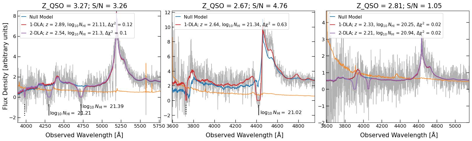
Figure 1: Three Ly$\alpha$CoLoRe quasar spectra (gray lines) and their simulated error spectra (orange lines) with the best fitting null model and n-DLA models that triggered a detection. The estimated $z$ and $N_{\texttt{HI}}$ of each detection is provided in the legends along with the $\Delta\chi_{r}^{2}$ of the fit. The solid vertical lines mark the location of true DLA troughs with the input $N_{\texttt{HI}}$ annotated. The dashed vertical lines indicate the corresponding true Ly$\beta$ troughs, if visible.

A DLA detection is defined using the threshold parameter $\Delta\chi_{r}^{2}$ in Equation (6). This term quantifies how much the fit improves (or degrades) from including a DLA absorption profile. It is always computed using the reduced $\chi^{2}$ to account for the extra parameters in an $n$-DLA model relative to a $(n-1)$-DLA model. To be maximally inclusive, the DLA Toolkit sets a weak threshold of $\Delta\chi_{r}^{2}>0.01$ to constitute a detection. In Section IV.1, we investigate alternative choices for the $\Delta\chi_{r}^{2}$ detection threshold.

$$\Delta\chi_{r}^{2}=\chi^{2}_{r,n-1}-\chi^{2}_{r,n}$$ (6)

If the $\Delta\chi_{r}^{2}$ for the 1-DLA model meets the detection threshold, we repeat the above procedure for a 2-DLA model and similarly for a 3-DLA model if merited. The solutions for any previously identified DLAs are fixed when solving subsequent models. The $\Delta\chi_{r}^{2}$ threshold for detection is uniform across all $n$. The DLA Toolkit stores the relevant information for each detection in an output catalog summarized in Table 1.

Figure 1 shows three simulated spectra in which the DLA Toolkit detected a candidate DLA. The first two panels show true positive detections while the last panel is an example false positive. Many false positives originate in low S/N spectra and from true high column density absorbers but with $N_{\texttt{HI}}$ below the search limit of the DLA Toolkit. The first false detection in the last panel of Figure 1 aligns with the position of a true absorber with input $z=2.33$ and $\log_{10}(N_{\texttt{HI}})=19.75$. As discussed in Section IV.1, the false positive rate can be mitigated with cuts on either S/N or $N_{\texttt{HI}}$.

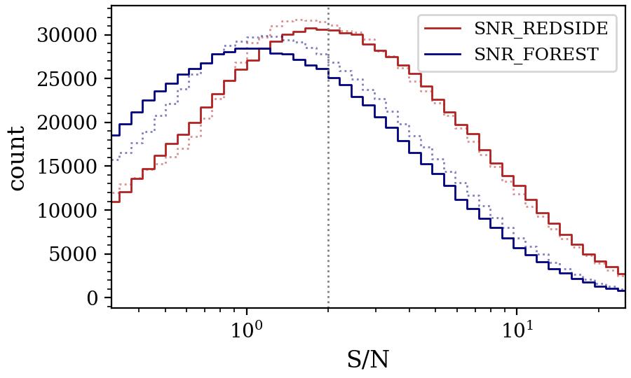
Figure 2: Histogram illustrating the SNR_REDSIDE and SNR_FOREST distributions for the DESI DR2 quasar (solid lines) sample and the Ly$\alpha$CoLoRe mock sample (dotted lines). The vertical dashed line indicates S/N $>2$.

III.1.1 S/N Metrics

The DLA Toolkit computes two S/N metrics that are saved in the code’s output. The first is SNR_REDSIDE which is defined by the average S/N per pixel over $1420\text{\AA }<\lambda_{RF,QSO}<1480\text{\AA }$. The second is SNR_FOREST which is defined by the average S/N per pixel over $1040\text{\AA }<\lambda_{RF,QSO}<1205\text{\AA }$. A value of $-1$ reflects insufficient wavelength coverage and is typically limited to SNR_FOREST for lower redshift quasars. The S/N distributions for the DESI DR2 quasar sample and the Ly$\alpha$CoLoRe mock data sample are shown in Figure 2. As evidenced in the figure, SNR_REDSIDE nearly always exceeds that computed in the forest by a factor of $1.5-2$, on average. This trend is exaggerated when a DLA is present [27, 28]. We exclusively use SNR_REDSIDE for any S/N value reported throughout this paper to avoid biasing against sightlines with DLAs.

IV Performance

We evaluate the DLA Toolkit on the sample of simulated spectra described in Section II.3 restricted to $2.0<z_{QSO}<4.25$. The lower limit ensures the Ly$\alpha$ forest is redshifted to the wavelength coverage of the DESI spectrographs while the upper limit comes from the the maximum quasar redshift used in the Ly$\alpha$ forest BAO measurement [39, 40]. Using the truth values for DLAs input into the mock spectra, we measure the column density and redshift accuracy of true positives. We then report on the purity and completeness of the resulting DLA sample and the dependence of these metrics on various parameters such as S/N. We perform identical tests with the GP and CNN DLA detection methods for comparison.

A persistent issue with DLA detection is BAL/DLA confusion. Since BAL contamination is removed before extracting Ly$\alpha$ flux transmission fields for BAO measurement [see the DESI BAL masking strategy presented by 74], we focus our validation on the BAL-free subset of the mock spectra sample. We include some discussion of performance on the full mock data sample, but all reported metrics and figures correspond to the BAL-free subsample unless explicitly stated otherwise.

IV.1 Validation on Simulated Spectra

We run the DLA Toolkit on the sample of approximately 930,000 simulated spectra that satisfy the quasar redshift restriction, of which $778,043$ are free of BALs. We trim the DLA Toolkit output catalog on predicted $\log_{10}(N_{\texttt{HI}})>20.3$ and remove flagged detections (see Section III.1). Approximately 13% of quasar sightlines have a DLA detection after applying these cuts, with $\sim$1% having multiple DLA detections.

The DLA truth catalog is defined as input DLAs with $\log_{10}(N_{\texttt{HI}})>20.3$ and redshifts within the wavelength search window defined by Equation (3) and Equation (4). A detection by the DLA Toolkit is considered a true positive if Equation (7) is uniquely satisfied for any DLA in the truth catalog. This is equivalent to the predicted DLA being within 3,000 km s^-1 of a true DLA.

$$\left|\frac{z_{\text{predicted}}-z_{\text{true}}}{1+z_{\text{true}}}\right|<0.01$$ (7)

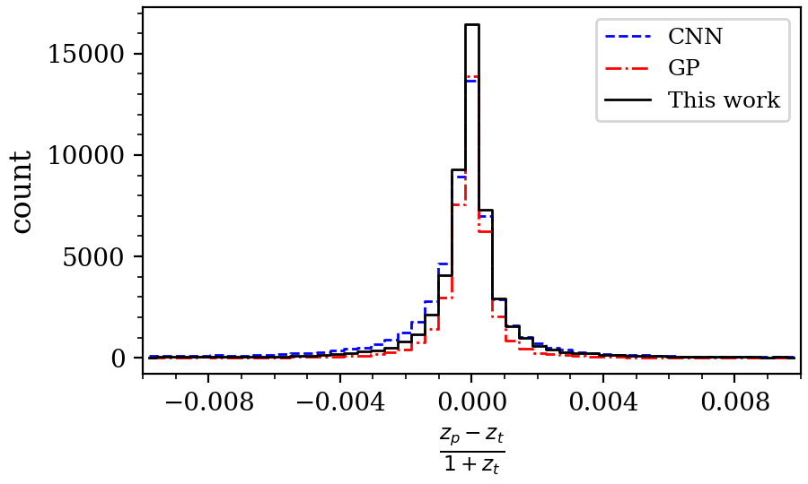
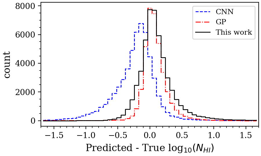
Figure 3: Histograms illustrating the parameter accuracy of the DLA Toolkit, GP DLA finder, and CNN DLA finder for the true positive $\log_{10}(N_{\texttt{HI}})>20.3$ detections. The top panel shows the offset of the predicted $z$ from truth. All methods have an average offset consistent with zero. The bottom panel shows the difference between predicted and true $\log_{10}(N_{\texttt{HI}})$ values. The average offset is $0.106$ for the DLA Toolkit, $0.076$ for the GP DLA finder, and $-0.219$ for the CNN DLA finder.

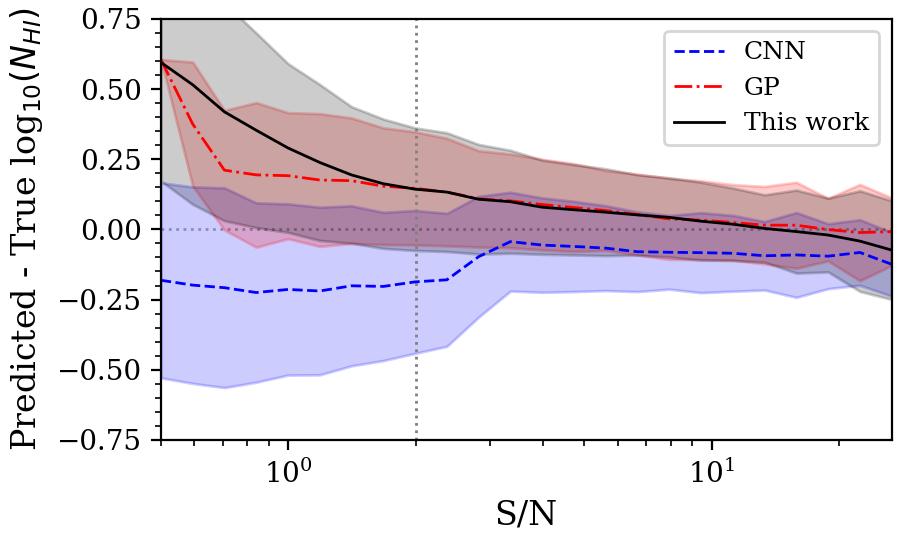
Figure 4: The average offset of predicted $N_{\texttt{HI}}$ from truth as a function of S/N for the DLA Toolkit, GP DLA finder, and CNN DLA finder for the true positive $\log_{10}(N_{\texttt{HI}})>20.3$ detections. The shaded regions are the standard deviation within each S/N bin. The vertical dashed line indicates S/N $>2$.

As shown in Figure 3, the majority of redshift estimates are accurate well within the boundary set by Equation (7), with an average offset consistent with zero. Figure 3 also indicates that the DLA Toolkit slightly over-predicts column density on average by $\Delta\log_{10}(N_{\texttt{HI}})=0.106~(\sigma=0.292)$. However, the $N_{\texttt{HI}}$ accuracy is S/N-dependent, and the average offset improves with increasing S/N as shown in Figure 4. When restricting to S/N $>2$, the average offset of column density from the truth value improves to $\Delta\log_{10}(N_{\texttt{HI}})=0.045~(\sigma=0.212)$.

The purity of the DLA sample is defined as the number of true positives divided by the number of all detections. The completeness is the number of true positives divided by the total number of DLAs in the truth catalog. We first assess how purity and completeness depend on the $\Delta\chi_{r}^{2}$ threshold for detection (see Equation (5)). We compute these metrics after cutting the catalog on $\Delta\chi_{r}^{2}>\Delta\chi_{r,min}^{2}$ for several values of $\Delta\chi_{r,min}^{2}$ spanning $0.01-0.25$. We only consider sightlines with a quasar S/N $>2$ since performance rapidly degrades below this. The S/N dependence is discussed in greater detail later in this section. As expected, the sample becomes more pure and less complete as the threshold $\Delta\chi_{r}^{2}$ increases, shown in Figure 5. We elect a detection threshold $\Delta\chi_{r}^{2}>0.03$, indicated by the star, in all further analyses to balance the purity and completeness tradeoff. This choice yields a sample that is 72.4% pure and 71.4% complete.

We next evaluate the dependence of purity and completeness on S/N with the detection threshold of $\Delta\chi_{r}^{2}>0.03$. As evidenced in Figure 6, the purity increases rapidly up to S/N $\approx 2$. The purity stabilizes beyond this point, increasing only moderately from $\sim$70% to $\sim$80%. We observe a similar rapid increase in completeness at S/N $<2$. In contrast to purity, completeness does not stabilize and actually begins to decrease around S/N $\approx 5$, particularly for S/N $\geq 10$. Approximately 22% of the truth DLA sample are in S/N $>5$ quasar spectra, where the average completeness of the DLA Toolkit is 70%. Roughly 8% of the truth DLAs are in quasar spectra with S/N $>10$, where the DLA Toolkit has an estimated purity of 60%. As such, the actual number of missed high S/N DLAs is relatively small compared to the full sample size. However, high S/N DLAs can have a substantial impact on the Ly$\alpha$ clustering measurements, so it is critical to understand why these DLAs are not detected and to recover them.

An analysis of these missing DLAs reveals an excess of flagged fits. In high S/N spectra, the DLA Toolkit often finds better solutions (in a $\chi^{2}$ sense) from fitting two lower column density DLA profiles to a single true DLA trough instead of one DLA profile with a larger, more accurate column density. These fits are flagged owing to their poor parabola fits and thus discarded by our cuts. These dual solutions to single DLA troughs are driven by local minima, indicating the $\chi^{2}$ relaxation process is less robust at the highest S/N. We discuss this failure mode and steps for potential remediation in Section VII.

Our final test checks the dependence of purity and completeness on DLA column density, shown in Figure 7. Since $N_{\texttt{HI}}$ accuracy is S/N dependent, we check the purity and completeness in bins on both parameters. For S/N $>2$ and $\log_{10}(N_{\texttt{HI}})>20.5$, purity nearly ubiquitously exceeds 70% and completeness is generally above 80%. As expected, we observe degraded performance at the lowest S/N and $N_{\texttt{HI}}$ values. The purity (completeness) is relatively low in the $20.3<\log_{10}(N_{\texttt{HI}})<20.5$ bins owing to scatter in the predicted $\log_{10}(N_{\texttt{HI}})$ values causing sub-DLAs (DLAs) to fall above (below) the 20.3 minimum requirement.

Lastly, when including BAL quasars in the test sample the DLA Toolkit achieves approximately the same completeness, but the purity decreases to 53.7% for $\Delta\chi_{r}^{2}>0.03$ and S/N $>2$. The trends for purity and completeness with S/N are relatively unchanged from the BAL-free sample, but they shifted to lower values in the case of purity. The $N_{\texttt{HI}}$ and $z$ accuracy are comparable to the BAL-free sample. Table 2 summarizes the purity and completeness metrics for both the full sample and the BAL-free sample.

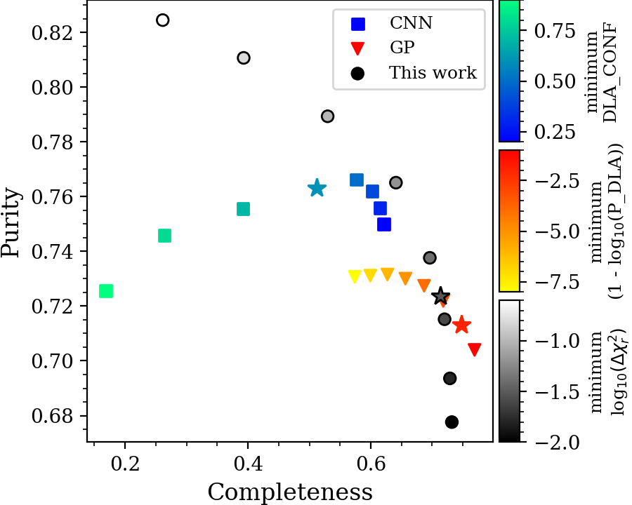
Figure 5: The purity and completeness of DLA samples for different cuts in detection confidence. The circle points correspond to the DLA catalog from the DLA Toolkit and are colored by the minimum $\Delta\chi_{r}^{2}$ to constitute a detection. The triangle (square) points correspond to the GP (CNN) DLA finder and are likewise colored by minimum P_DLA (DLA_CONFIDENCE) for detection. All DLA samples are limited to S/N $>2$ and predicted $\log_{10}(N_{\texttt{HI}})>20.3$. The stars are the thresholds for the DESI DR2 BAO measurement.

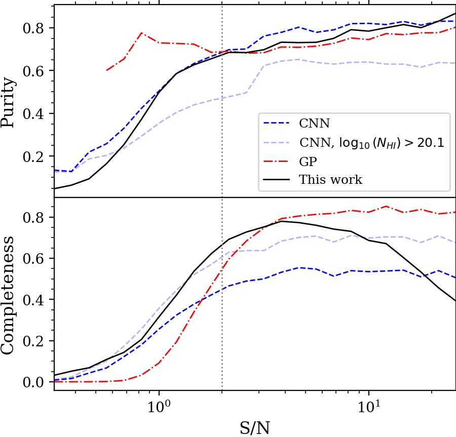
Figure 6: The purity and completeness of DLA samples as a function of S/N from the DLA Toolkit, GP DLA Finder, and CNN DLA finder. The samples are cut on confidence and predicted $\log_{10}(N_{\texttt{HI}})>20.3$, except the alternative CNN line as annotated. The vertical dashed line indicates S/N $>2$.

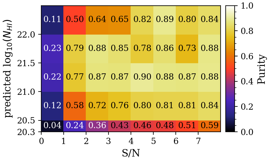
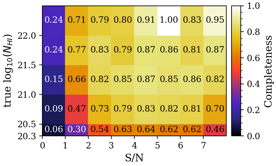
Figure 7: Purity (left) and completeness (right) values with the DLA Toolkit for different S/N and $\log_{10}(N_{\texttt{HI}})$ bins. The $\log_{10}(N_{\texttt{HI}})>22.0$ bins contain $\leq 35$ objects each. The $5<$ S/N $<6$, $\log_{10}(N_{\texttt{HI}})>22.0$ bin with 100% completeness contains only 7 DLAs.

This Work GP CNN Combined $\Delta\chi_{r}^{2}>0.03$ P_DLA $>0.99$ DLA_CONF $>0.6$ Purity 72.4% 71.3% 76.3% 76.2% Purity (BAL) 53.7% 48.0% 59.4% 59.7% Comp. 71.4% 74.7% 51.1% 71.1% Comp. (BAL) 69.9% 74.7% 50.4% 69.9%

Table 2: The purity and completeness of DLA samples from the DLA Toolkit, GP DLA Finder, CNN DLA Finder, and the combination of the three methods (as outlined in Section VI) for the Ly$\alpha$CoLoRe mock spectra sample. All DLA samples are from quasar spectra with S/N $>2$ and have predicted $\log_{10}(N_{\texttt{HI}})>20.3$.

IV.2 Comparison to other DLA algorithms

The GP DLA finder from Ho et al. [33] and the CNN DLA finder from Wang et al. [22] were used in conjunction to identify DLA contamination in the DESI DR1 Ly$\alpha$ forest BAO measurement [39]. The current version of the GP model was trained on quasar spectra from the extended Baryon Acoustic Oscillation Survey [eBOSS; 78]. The current CNN version was trained on simulated quasar spectra mimicking the first year of observations with the DESI survey. We run these DLA finders on the same simulated quasar sample that was used to evaluate the DLA Toolkit in Section IV.1 and compare their performances. We refer the reader to [33, 22] for complete details on these two methods.

To ensure analogous results from each technique, we perform a series of cuts on the output DLA catalogs from the GP and CNN DLA finders on the Ly$\alpha$CoLoRe mocks. We remove detections with predicted $\log_{10}(N_{\texttt{HI}})<20.3$ and restrict the DLA redshift range to that defined by Equation (3) and Equation (4). We then remove any detections flagged as problematic by the GP. The CNN does not maintain any flags, so we retain all detections from this algorithm that pass the redshift and column density cuts. As with the DLA Toolkit, we consider a GP or CNN DLA detection a true positive if the predicted redshift uniquely satisfies Equation (7) for any DLA in the $\log_{10}(N_{\texttt{HI}})>20.3$ truth catalog.

Figure 3 illustrates that, on average, the GP and CNN methods achieve equally precise redshift estimates as the DLA Toolkit. The average offset of the predicted GP and CNN redshifts from truth is consistent with zero, similar to what was reported by [22]. The GP, however, produces a tighter distribution for the offset of predicted $N_{\texttt{HI}}$ values from truth than either the CNN or the DLA Toolkit. The average offset of GP predicted column density from truth is $\Delta\log_{10}(N_{\texttt{HI}})=0.076~(\sigma=0.203)$. The CNN, in contrast, provides the least reliable column density predictions of the three methods, on average, with a mean offset of $\Delta\log_{10}(N_{\texttt{HI}})=-0.219~(\sigma=0.485)$ [34, 35, previously reported a bias on column density].

We next compare the dependence of $N_{\texttt{HI}}$ accuracy on S/N for the three methods in Figure 4. The DLA Toolkit and GP tend to overestimate $N_{\texttt{HI}}$ in a relatively similar fashion that improves with increasing S/N. This may be a consequence of the difficulty in modeling intrinsic quasar continua at lower S/N, which both approaches rely on when estimating column density. Meanwhile, the CNN tends to underestimate $N_{\texttt{HI}}$ by a consistent average magnitude of $\Delta\log_{10}N_{\texttt{HI}}\approx 0.08$ at S/N $>3$ and $\Delta\log_{10}N_{\texttt{HI}}\approx 0.205$ at S/N $<2$. It is clear that $N_{\texttt{HI}}$ accuracy is degraded for all methods at low S/N. Applying a lower limit S/N $>2$, the average offset of column density from the truth value improves to $\Delta\log_{10}(N_{\texttt{HI}})=0.061~(\sigma=0.192)$ for the GP and $\Delta\log_{10}(N_{\texttt{HI}})=-0.161~(\sigma=0.235)$ for the CNN. Figure 4 also makes it apparent that the improved average $N_{\texttt{HI}}$ accuracy of the GP over the DLA Toolkit arises in the S/N extremes (S/N $\lesssim 1.5$ and S/N $\gtrsim 18$).

The GP and CNN DLA finders both have an output variable that quantifies detection significance for candidate DLAs, similar to the DLA Toolkit’s $\Delta\chi_{r}^{2}$. The GP reports a P_DLA value, and the CNN reports a DLA_CONFIDENCE value for each detection. Both parameters are on a scale of zero to one where larger values correspond to higher confidence. P_DLA exhibits a rather bimodal distribution, returning values greater than 0.9 or equal to zero. The latter is equivalent to a non-detection. For the CNN, the distribution of detections generally decreases with increasing DLA_CONFIDENCE value, aside from a spike of detections with DLA_CONFIDENCE $=1.0$.

Figure 5 demonstrates how the purity and completeness of the GP and CNN DLA samples depend on their respective detection thresholds. In general, the GP can achieve the highest completeness of the three algorithms whereas the DLA Toolkit can provide the best purity. The behavior of the CNN as the threshold DLA_CONFIDENCE increases suggests that DLA_CONFIDENCE is not necessarily a good indicator of DLA probability. We define a DLA detection by P_DLA $>0.99$ for the GP and DLA_CONFIDENCE $>0.6$ for the CNN. Using these thresholds, the GP provides a DLA sample that is 71.3% pure and 74.7% complete, and the CNN provides a DLA sample that is 76.3% pure and 51.1% complete.

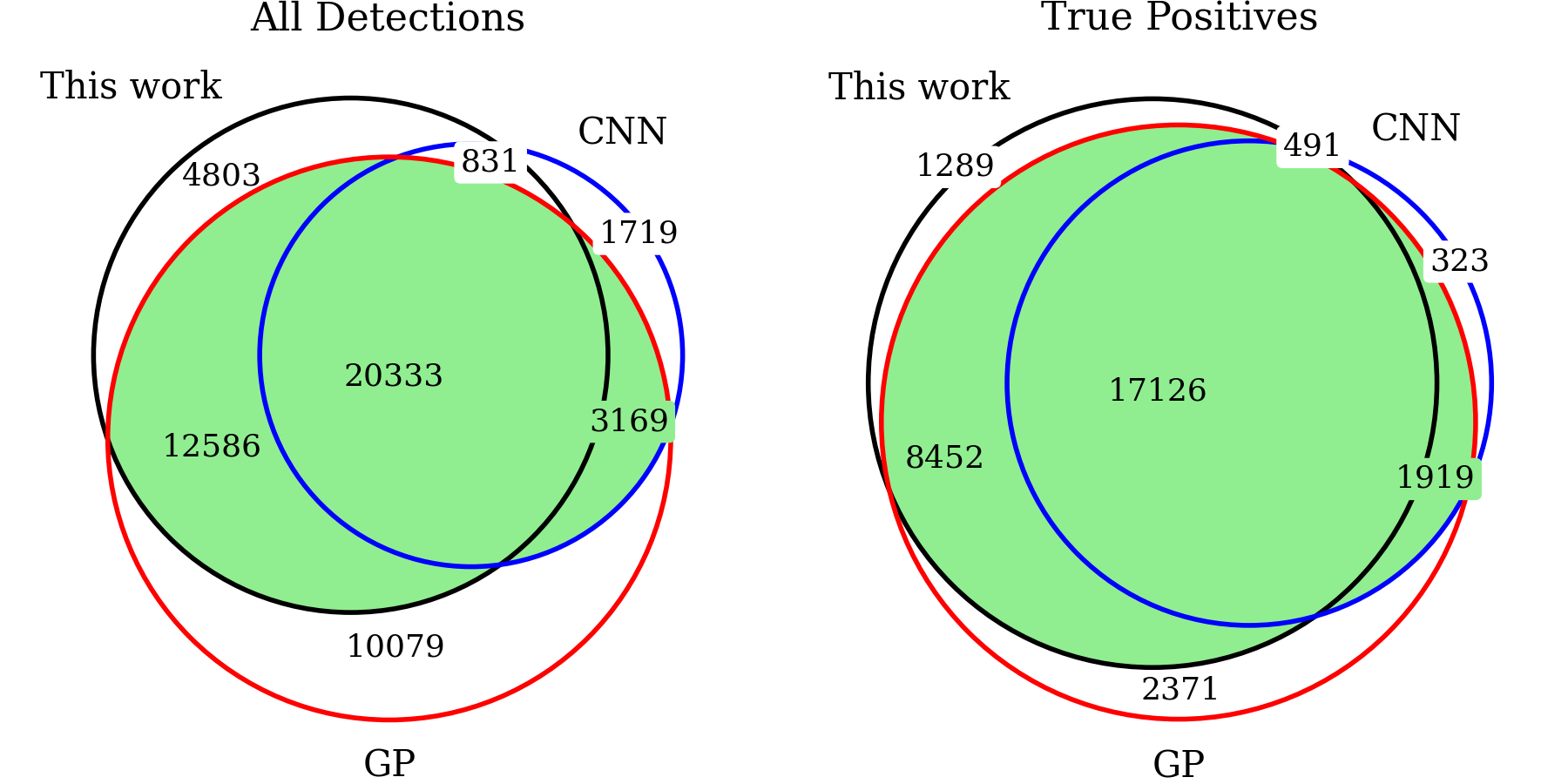
Figure 8: Venn diagram of all detections (left) and the true positive detections (right) by the DLA Toolkit, GP, and CNN methods where S/N $>2$. These detections are required to meet $\Delta\chi_{r}^{2}>0.03$, P_DLA $>0.99$, and/or DLA_CONFIDENCE $>0.6$ depending on method. We also require $\log_{10}(N_{\texttt{HI}})>20.3$. The green shaded region represents the detections selected by Equation (11).

The top panel of Figure 6 shows how the purity of these samples depends on S/N with the chosen detection thresholds. The GP purity is nearly constant at $\sim$70% for S/N $>0.5$, but reports no detections below this. The lack of low-S/N detections may be driven by inadequate training of the GP model on noisy data. Since the GP relies on a Bayesian framework, its predictions become prior-driven when the model lacks sensitivity to certain data regimes, i.e., favoring non-DLA detection by default. The CNN exhibits a similar trend in purity to the DLA Toolkit but is up to $\sim$10% more pure at the S/N $<1$ and $\lesssim 5\%$ more pure between $3<\text{S/N}<13$.

The trends of completeness with S/N are shown in the bottom panel of Figure 6. Above S/N $>2$, both the GP and CNN achieve roughly uniform completeness of approximately 80% and 50%, respectively. The DLA Toolkit outperforms the GP and CNN at S/N $<4$, after which the GP provides the most complete DLA sample. A summary of the purity and completeness metrics for the GP and CNN DLA finders is given Table 2.

The low completeness of the CNN reported in this work is likely driven by its systematic underestimation of $N_{\texttt{HI}}$. We show in Figure 6 that relaxing the column density threshold to predicted $\log_{10}(N_{\texttt{HI}})>20.1$ can boost the CNN’s completeness but at the cost of lower purity. With this lower $N_{\texttt{HI}}$ minimum, the purity (completeness) decreases (increases) $\sim 20\%$ above S/N$>2$. Since the focus of this work is identifying DLA contamination for BAO, we choose to keep the $\log_{10}(N_{\texttt{HI}})>20.3$ cut-off to minimize the loss of uncontaminated forest regions. Further, we expect the GP and DLA Toolkit will compensate for CNN in this regime (see Section VI). We refer the reader to [34] and [35] for discussions on de-biasing $N_{\texttt{HI}}$ from the CNN, but caution that de-biasing procedures should be updated to reflect the new training [22]. We leave more sophisticated work on de-biasing the CNN $N_{\texttt{HI}}$ and subsequent effects on DLA detections to future works.

Differences in our reported performance metrics compared to Wang et al. [22], who evaluated both the GP and CNN methods on DESI DR1 mock spectra, are likely due to a combination of factors. First, the DESI DR2 mocks used in this study feature improved realism relative to the mock spectra used in their analysis [see 42, for details on the mock improvements]. We also do not consider subDLA column densities ($\log_{10}N_{\texttt{HI}}<20.3$) in our assessment, whereas the DLA samples in [22] are defined by $\log_{10}N_{\texttt{HI}}>20.0$. The lower column density threshold results in a substantially larger sample size than with the canonical DLA column density cut-off used in this work. We additionally find larger offsets of predicted $N_{\texttt{HI}}$ from truth than was reported by [22], particularly for the CNN method, even when restricting to S/N $>3$. Finally, we use a lower S/N cut-off and higher detection significance thresholds for both methods for our final catalog, informed by the results of our analyses.

Finally, we look at the overlap between the DLA catalogs produced by the DLA Toolkit, GP, and CNN methods for $\log_{10}(N_{\texttt{HI}})>20.3$ detections. Motivated by the previous tests, we require $\Delta\chi_{r}^{2}>0.03$, P_DLA $>0.99$, DLA_CONFIDENCE $>0.6$, and S/N $>2$. We associate detections between catalogs if they have predicted $z$ values within 800 km s^-1, following the convention of [39, 37].

The distribution of candidate DLAs found by at least one of the DLA Toolkit, GP, or CNN methods is shown on the left in Figure 8 while the right shows the subset which are true DLAs. The largest subset of candidate DLAs shown in Figure 8 corresponds to those detected by all three methods. This subset has a high purity of 84.2%, demonstrating how combining techniques helps to filter out contamination from the individual catalogs. The next largest subset is candidate DLAs detected by the DLA Toolkit and the GP method with a purity of 67.2%. After this, the next largest subset is candidate DLAs detected by only the GP method with a purity of 23.5%. The two subsets corresponding to shared GP and CNN candidate DLAs or shared DLA Toolkit and CNN candidate DLAs are relatively smaller but have 60.6% and 59.1% purity, respectively. These results suggest that while detections made by all three methods are the most pure, each method contributes unique identifications, highlighting the importance of using multiple approaches for a more comprehensive DLA catalog.

V DLA Catalogs from the DLA Toolkit

We run the DLA Toolkit on the quasar samples from DESI DR1 and DR2 described in Section II.2, restricting both samples to $2.0<z_{QSO}<4.25$. Flagged detections are removed from the output catalogs and therefore not considered in the statistics reported in the following subsections. We refer the reader to the performance metrics reported in Section IV.1 as a guideline for selecting and using DLA samples from these catalogs. Since simulated spectra cannot capture the full diversity observed in real quasar spectra, the purity and completeness measurements should be treated as approximate. Candidate DLAs can be matched via TARGETID to the corresponding quasar catalog to remove BAL sightlines and enhance the sample purity.

V.1 The DR1 Catalog

After applying the quasar redshift cut, the DR1 sample consists of 520,745 sightlines. The DLA Toolkit records 74,918 detections for this sample, of which 60,565 have predicted $\log_{10}N_{\texttt{HI}}>20.3$. Approximately 1% of quasar sightlines contain more than one candidate DLA.

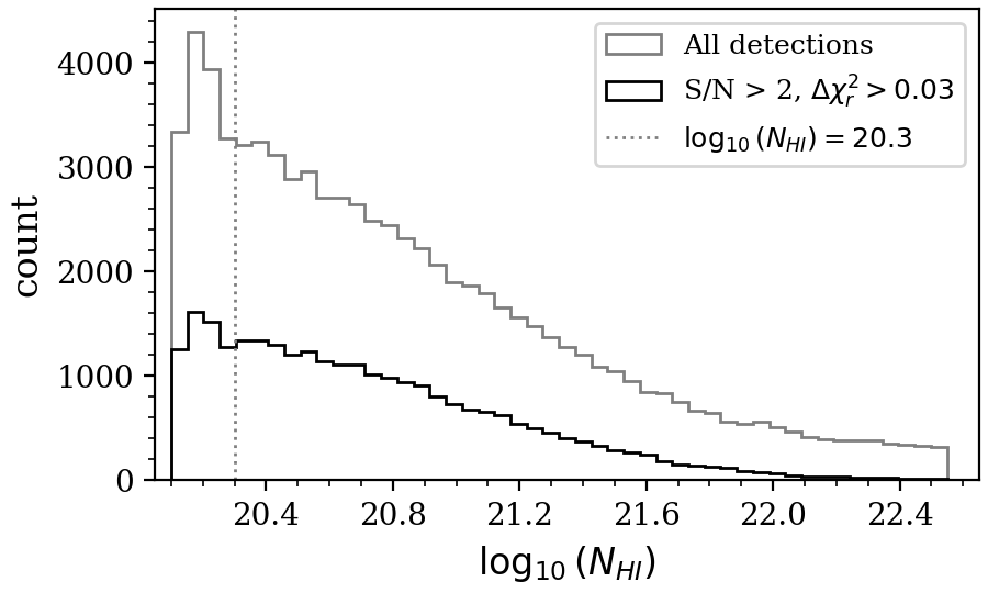
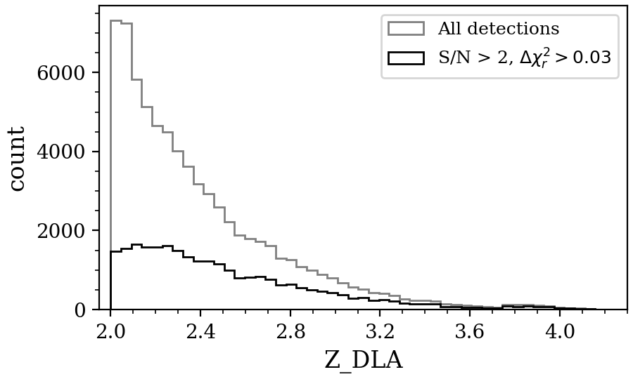
Figure 9: The predicted redshift and $\log_{10}(N_{\texttt{HI}})$ distribution of the DLA Toolkit catalog for DESI DR1. The vertical line is the DLA column density definition.

The best performance is expected for S/N $>2$, as evidenced throughout Section IV.1. Using this S/N limit and a $\Delta\chi_{r}^{2}>0.03$ threshold, 26,651 DLA candidates remain in the catalog with 21,173 having predicted $\log_{10}N_{\texttt{HI}}>20.3$ (from 235,856 S/N $>2$ sightlines). Figure 9 shows the distribution of predicted column density and redshift for the full sample and the sample optimized with S/N and $\Delta\chi_{r}^{2}$ cuts.

The DR1 DLA catalog from the DLA Toolkit, along with the corresponding quasar catalog, is available concurrently with the full DESI DR1 [38]. The DLA catalog contains the information summarized in Table 1. The catalog complements the concordance DLA catalog presented in the forthcoming paper by [37], which includes DLAs found with the CNN and GP methods.

V.2 The DR2 Catalog

The DESI DR2 sample contains 942,946 quasar sightlines that satisfy $2.0<z_{QSO}<4.25$. The DLA Toolkit returns 137,222 candidate DLAs with predicted $\log_{10}(N_{\texttt{HI}})>20.3$. Restricting to the S/N $>2$ (455,360 quasar sightlines) leaves 66,955 candidate DLAs with predicted $\log_{10}(N_{\texttt{HI}})>20.3$ remaining in the sample. Further limited to detections with $\Delta\chi_{r}^{2}>0.03$ results in an optimized sample of 52,575 candidate DLAs. Similar to the DR1 catalog, roughly 1% of sightlines have more than one candidate DLA.

VI The DR2 Combined Catalog for Lyman-Alpha Forest BAO

This section presents the construction of the DLA catalog for the DR2 Ly$\alpha$ forest BAO measurement [40]. The wings of DLA absorption profiles, which can extend for thousands of km s^-1, not only compromise the ability to extract the neutral hydrogen density field but increase noise in the correlation function and alter its broadband shape [e.g. 19]. DLAs also cluster more strongly than the Ly$\alpha$ forest [e.g. 9, 16, 17], increasing the bias of the correlation function. It is essential to efficiently identify DLAs for the BAO analysis, so they may be masked and their impact on the correlation function mitigated. We combine output DLA catalogs from the GP, CNN, and DLA Toolkit on the DESI DR2 quasar sample to construct a highly complete and pure catalog. We aim to optimally balance these two metrics as to reduce contamination without erroneous loss of forest pixels.

We combine output catalogs from the CNN and GP DLA finders on the DR2 quasar sample with the DLA Toolkit catalog from Section V.2 as follows. To begin, we match candidate DLAs between catalogs within 800 km s^-1. We then remove detections from each method that do not meet the $\log_{10}(N_{\texttt{HI}})>20.3$ or confidence minimums. The chosen confidence minimums per method are informed by the results presented in Section IV. We also require S/N $>2$ since we expect degraded performance from all three algorithms at low S/N. In summary, detections ($det_{i}$) from each algorithm are defined following Equations (8), (9), and (10). The number of candidate DLAs satisfying the detection criterion for each method is given in Table 3.

$$det_{\texttt{Toolkit}}= (\log_{10}(N_{\texttt{HI-Toolkit}})>20.3)$$ (8)

$$\cap(\Delta\chi_{r}^{2}>0.03)\cap(\text{S/N}>2)$$

$$det_{\texttt{GP}}= (\log_{10}(N_{\texttt{HI-GP}})>20.3)$$ (9)

$$\cap(\texttt{P\_DLA}>0.99)\cap(\text{S/N}>2)$$

$$det_{\texttt{CNN}}= (\log_{10}(N_{\texttt{HI-CNN}})>20.3)$$ (10)

$$\cap(\texttt{DLA\_CONFIDENCE}>0.6)\cap(\text{S/N}>2)$$

Based on the catalog overlap discussion in Section IV.2, the final combined catalog requires a detection by both the GP and either one of the DLA Toolkit or the CNN. This decision aims to maximize completeness without sacrificing purity. The GP detection then sets the final predicted redshift and column density so that all candidate DLAs use a common z and $N_{\texttt{HI}}$ estimator. Equation (11) summarizes the logic for constructing the combined catalog. The final catalog has 41,152 candidate DLAs. We note that this catalog does not remove BAL sightlines.

$$det_{\texttt{Combined}}=det_{\texttt{GP}}\cap(det_{\texttt{Toolkit}}\cup det_{\texttt{CNN}})$$ (11)

Total Candidate DLAs non-BAL sightlines DLA Toolkit 52,575 35,939 GP 69,995 32,100 CNN 52,072 25,457 Combined 41,152 25,568

Table 3: Number of candidate DLAs found in the DESI DR2 quasar sample by each method following the definitions in Equations (8)$-$(11).

To assess the expected purity and completeness of the combined catalog, we apply Equation (11) to the mock DLA catalogs presented in Section IV from the DLA Toolkit, GP, and CNN methods. For this analysis, we exclude BAL sightlines since that type of contamination is removed separately by [40] in the BAO measurement. DLA detections satisfying Equation (11) are shown as the green shaded area in Figure 8. It has a purity of 76.2% and a completeness of 71.1%. These metrics are included in Table 2 for comparison to the catalogs from the individual methods. We validate our mock estimated purity with data stacks in Section VI.1.

We considered an alternative combination strategy that requires detection by any two of the methods. This choice slightly increases (decreases) the completeness (purity) of the sample, as illustrated in Figure 8; However, requiring a common method across all candidate DLAs in the combined catalog allows us to standardize the parameter predictions. The GP is the best choice for the common method owing to its greater $N_{\texttt{HI}}$ accuracy relative to the other two methods and its high completeness.

We also evaluated the DR1 BAO strategy which required $\texttt{CNN\_CONFIDENCE}>0.5$ and $\texttt{P\_DLA}>0.5$ for building a combined DLA catalog for DR2. With these thresholds, we get 81.2% purity and 56.4% completeness at S/N $>2$. This catalog’s redshift and column density accuracy are identical to our presented strategy since both use the GP solutions for the final predictions. Thus, this new DR2 strategy increases completeness by adding $\sim 15\%$ while only losing $\sim 5\%$ in purity.

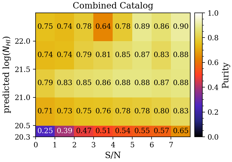
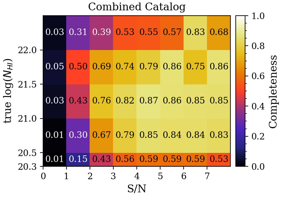
Figure 10: The purity (left) and completeness (right) of the combined catalog constructed following Equation (11) with the individual catalogs from the DLA Toolkit, GP, and CNN methods on the mock data sample presented in Section IV.

As a final analysis of the combined catalog using mock spectra, we evaluate purity and completeness in the same S/N and $\log_{10}(N_{\texttt{HI}})$ bins as in Figure 7 for the DLA Toolkit. These results are shown in Figure 10. The relatively low completeness at high $N_{\texttt{HI}}$ is due to a combination of factors: a known issue where the DLA Toolkit (and GP method) can fit two lower-$N_{\texttt{HI}}$ DLA profiles instead of one higher-$N_{\texttt{HI}}$ DLA profile to a single trough (discussed in Section IV.1 and Section VII), and the strict requirement that matched DLAs between catalogs must fall within 800 km s^-1. Relaxing this criterion to 3,000 km s^-1, as done for determining true positives with Equation (6), substantially improves completeness at high $N_{\texttt{HI}}$. Appendix A presents the impact of this alternative matching criterion in more detail.

VI.1 Purity Validation with Spectral Stacking

Spectroscopic stacking is a common tool for the study of well-understood absorber samples. Pieri [79] and Frank et al. [80] also showed that one can stack mixed samples of apparent absorption and, using the basic rules of atomic physics and spectroscopy, learn the mix of ionization species and noise that gave rise to the sample. In those articles lines were stacked to determine whether they were caused by metal doublets via the deviation from the normal 2:1 line ratio. In effect, one can test the purity with which the apparent lines found are any desired metal doublet.

Here we use the Lyman series in place of metal doublets. We use the fact that all DLAs with a column density $\log_{10}(N_{\texttt{HI}})>20.3$ should show no transmission at the line center for at least the first 10 Lyman series lines [81, 82], even at DESI resolution. By construction, any Lyman series lines included in a DLA identification process will show no (or nearly no) transmission, but any Lyman series lines not included are available for this test of purity. However, a subtlety remains that must be accounted for; the typical contaminants of DLA samples are large complexes of strong Ly$\alpha$ forest absorption (along with noise). The Lyman series absorption associated with these complexes depends on the mix of column densities for each interloper. These complexes may show strong absorption at Ly$\alpha$ but as one moves up the Lyman series they converge to an expectation value of 100% transmission. In a stack with a mix of real DLAs and these interlopers, the mean transmission at line center must increase as one moves up the Lyman series to asymptote to a constant value corresponding to a mixture of DLAs with 0% expected transmission and interlopers with 100% expected transmission. This procedure has been tested with mock spectra and appears to be unaffected by DLA redshift errors for all classifiers discussed here.

In the work that follows, this asymptote appears to occur at Lyman-8, such that Lyman-9 and Lyman-10 generate consistent results within the limits of the signal-to-noise of the stacked spectrum. Hence the purity of the stacked DLA sample is given by the measured flux decrement ($1-F$) divided by the expected flux decrement at Lyman-8 (unity).

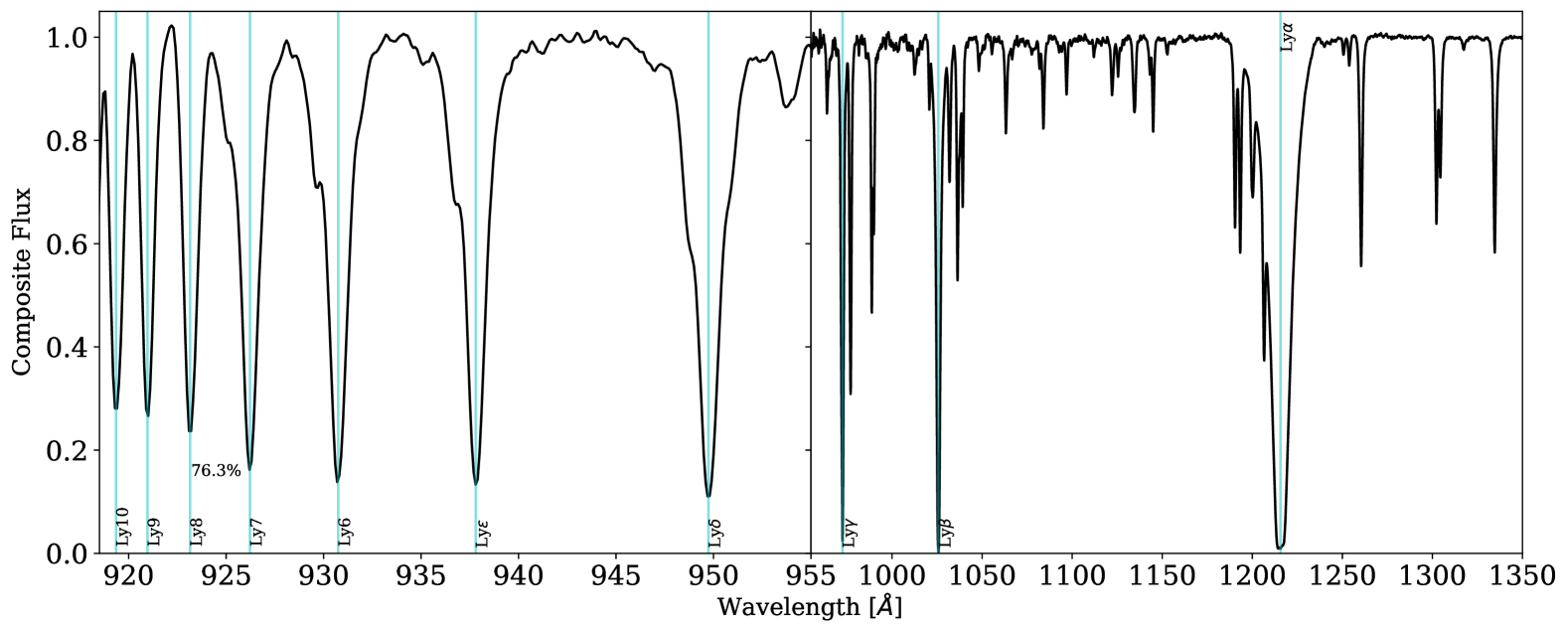
Figure 11: Composite spectrum of DLAs in the DR2 Combined Catalog, according to the properties defined in Section VI.1. Lyman series lines are marked with vertical cyan lines. The percentage close to the Lyman-8 line represents the purity in the selected DLA sample for predicted $z\gtrsim 2.9$.

The stacking procedure goes as follows: firstly, we choose which DLAs to stack. In this case, we chose absorbers in the DR2 combined catalog defined by Equation (11), removing quasar sightlines flagged for BAL features. We require the DLA to lie between 911 Å and 1205 Å in the quasar’s rest frame. The Lyman-8 absorption line redshifts into the DESI spectrograph wavelength coverage ($\lambda_{min}=3600$ Å) for candidate DLAs with predicted $z\gtrsim 2.9$. As such, we only measure the purity of the subset with predicted $z\gtrsim 2.9$, corresponding to $\sim$22% of the combined catalog after BAL sightlines were excluded. As a result, our test includes relatively few DLAs in the Ly$\beta$ forest and is a somewhat conservative estimation of DLA purity in the entire sample (since the forest opacity is higher at higher redshift and so DLA interlopers are more common).

After defining our sample for stacking, we choose a grid upon which to interpolate the data. In this case, we chose a grid spanning 910 Å to 1350 Å (to capture the Lyman Limit), with a periodicity of 0.25 Å. We chose this interval as it approximately matches the 0.8 Å spacing of the DESI spectrographs [52] redshifted to the DLA rest frame.

Next comes the stacking itself. For each DLA, we shift the wavelength solution of its corresponding spectrum to the absorber rest frame, which is set by the predicted redshift from the GP for the combined catalog. The spectrum is then continuum normalized, and the flux and inverse variance are interpolated onto the stacking grid we defined beforehand. The mean value of the flux and inverse variance are calculated, giving rise to the stack. We perform a pseudo-continuum fit on the stack, allowing us to correct for systematic errors in the continuum fits as well as remove undesirable features from uncorrelated absorption [83]. To get this pseudo-continuum, we perform a simple spline fit of the stack.

The final composite spectrum is shown in Figure 11. The purity estimate we obtain from the Lyman-8 flux decrement is 76.3%. Though the stacking probes a restricted redshift range, this measurement is remarkably similar ($<1\%$ different) to that from the mock analysis given in Table 2. We repeat this analysis on the DLA sample from the DLA Toolkit only (Section V.2), which can be seen in Appendix B.

VII Future Outlook

The impact of DLA masking on BAO using the various DLA catalogs presented in this work is explored by Casas et al. [42]. The authors demonstrate that BAO parameters remain highly robust against minor variations in the $N_{\texttt{HI}}$ threshold, purity, and completeness. For example, they show that the individual catalogs from the DLA Toolkit, GP, and CNN methods as well as the final combined catalog produce consistent BAO results with similar uncertainties (see their Figures 12 and 13). While BAO is robust to variation in DLA catalog, other Ly$\alpha$ forest analyses may benefit from adopting alternative catalog strategies than that presented in Section VI to improve performance in the $N_{\texttt{HI}}$ extremes. In particular, the Ly$\alpha$ forest full shape, 1-dimensional power spectrum, and 3-dimensional power spectrum analyses are more sensitive to DLA contamination than BAO [e.g. 24, 21] and would benefit from improved completeness. In Appendix A, we show that relaxing the redshift matching criterion between catalogs can boost completeness at $\log_{10}N_{\texttt{HI}}>22.0$ by up to 30%. Meanwhile, the performance outside of this regime is stable at the 1% level against this change. While DLAs of this high column density are rare, they do compromise a significant fraction of the forest when present.

The completeness at lower $N_{\texttt{HI}}$ could also be improved by applying the minimum column density cut at a later point in the combined catalog’s construction. Since predicted $N_{\texttt{HI}}$ from the CNN is negatively biased, we considered cutting the combined catalog on predicted $\log_{10}(N_{\texttt{HI}})>20.3$ from the GP only. This is similar to the approach by [37] and provides a catalog that is 75.3% complete (4.2% higher); however, the purity decreases to 69.8% (6.4% lower). The change in these metrics relative to Section VI is driven by detections with $20.3<\log_{10}(N_{\texttt{HI}})<20.5$.

Our purity and completeness analysis for the DLA Toolkit, GP, and CNN illustrates some of the strengths and weaknesses of each algorithm. As it is a major focus of this paper, we discuss specific modifications to the DLA Toolkit that could improve performance.

The most notable DLA Toolkit failure mode is the low completeness at high S/N. This is primarily driven by poor $\chi^{2}$ relaxation on the ($N_{\texttt{HI}}$, $z$)-surface owing to local minima within true DLA troughs. As such, the DLA Toolkit often returns 2 DLA solutions corresponding to a single true DLA, each with low predicted $N_{\texttt{HI}}$. Future code releases will particularly target the high S/N regime for improvement. Potential solutions are altering the procedure for $\chi^{2}$ surface relaxation such that local minima traps are disfavored. For example, the step size of $N_{\texttt{HI}}$ and $z$ can decrease with increasing SNR to retain an efficient runtime while allowing for a more detailed search at high SNR. Alternatively (or additionally), a minimum $\Delta z$ restriction can be imposed between DLAs on the same sightline to discourage multiple solutions for the same DLA or it can be used as a trigger to refit the parabola with a wider refined search window.

Another path to enhance performance is a replacement of the quasar flux model with one trained on DESI quasar spectra. The current quasar model, introduced in Section III.1, was trained on SDSS quasars. The bluest wavelengths of SDSS spectra suffer from poor spectrophotometric calibration [84] therefore, we may expect degraded modeling performance in exactly the wavelength region in which we are looking for DLAs. Ongoing work related to upgrading the quasar model shows promising results, specifically in regards to improved predicted $N_{\texttt{HI}}$.

As for the GP and CNN DLA finders, there is ongoing work to retrain both methods on the higher-quality spectra that are now available with DESI. The CNN model is being reconstructed and retrained on the new generation of DESI mocks that feature improved realism. For the GP, DESI DR2 data is being used to upgrade the null model with the specific intent of improving its ability to distinguish between DLA and non-DLA sightlines in the low-S/N regime.

VIII Summary

In this work, we presented the DLA Toolkit software for automated DLA detection. The technique uses a spectral template fitting approach that identifies DLA positions and estimates their column densities via sliding Voigt profiles while accommodating variance in the quasar’s flux. We explore the performance of the DLA Toolkit with respect to S/N, $N_{\texttt{HI}}$, and detection confidence as defined by the $\chi^{2}$ parameter in Equation (5) on a sample of simulated mock spectra. The best performance is achieved for S/N $>2$, and we recommend applying a $\Delta\chi^{2}>0.03$ cut to enhance purity. With these cuts, the mock DLA sample from the DLA Toolkit is over 70% pure and complete for non-BAL sightlines and the predicted redshifts are highly accurate. The DLA Toolkit tends to overestimate column densities with an accuracy that generally improves with S/N. We make available a catalog of candidate DLAs found with this technique on DESI DR1.

We combined the DLA catalog from the DLA Toolkit with catalogs from the GP DLA finder by Ho et al. [33] and the CNN DLA finder by Wang et al. [22] on the DESI DR2 quasar sample from the Ly$\alpha$ forest BAO analysis presented in [40]. Our charge is constructing a DLA catalog for the Ly$\alpha$ BAO analysis that optimally balances purity and completeness such that DLA impact on BAO parameter uncertainty is minimized. The combined catalog prescription is presented in Section VI, summarized by Equations (8)$-$(11). Given the performance of all three methods degrades at low S/N, we restrict our combined catalog to S/N $>2$ to avoid unnecessary loss of Ly$\alpha$ signal. We additionally require predicted $\log_{10}N_{\texttt{HI}}>20.3$ owing to the difficulty of accurately identifying high column density absorbers below this. The DLA parameters of the combined catalog are determined by the GP DLA finder, which provides the highest accuracy predicted $N_{\texttt{HI}}$ (Figure 3) of the three algorithms.

An analysis of the combined catalog strategy on mocks suggests the combined DLA catalog for DR2 Ly$\alpha$ BAO is 76.2% pure and 71.1% complete when BAL sightlines are excluded. Compared to the DLA catalog strategy used for DR1 Ly$\alpha$ BAO, this constitutes an improvement of roughly 15% in completeness while losing only 5% in purity. When BAL sightlines are included, the purity estimate drops to 59.7% with a relatively stable completeness of 69.9%. Lastly, we obtain an estimate for purity of 76.8% on real data through spectral stacking of the combined catalog for DR2 Ly$\alpha$ BAO.

Data Availability

The DLA catalog from the DLA Toolkit for data collected during DESI DR1 observations is available at https://data.desi.lbl.gov/public/dr1/vac/dr1/dla-toolkit. All data shown in figures can be downloaded from https://doi.org/10.5281/zenodo.14948183.

Appendix A Relaxed Redshift Matching Between Catalogs

As discussed in Section VI, the strategy for combining the DLA catalogs from the DLA Toolkit, GP, and CNN methods results in relatively low completeness for DLAs with $N_{\texttt{HI}}>22.0$ (see Figure 10). One contributing factor is the decision to associate DLA detections from different methods only if they fall within 800 km s^-1 of each other, following [39, 37].

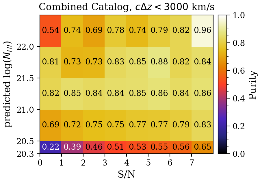
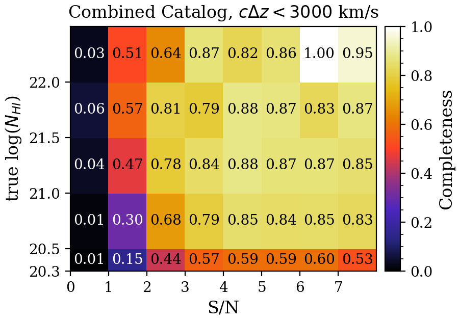
Figure 12: The purity (top) and completeness (bottom) of the combined catalog when relaxing redshift matching criteria to within 3,000 km s^-1 as function of S/N and $\log_{10}(N_{\texttt{HI}})$. The $6<$ S/N $<7$, $\log_{10}(N_{\texttt{HI}})>22.0$ bin with 100% completeness contains only 6 DLAs.

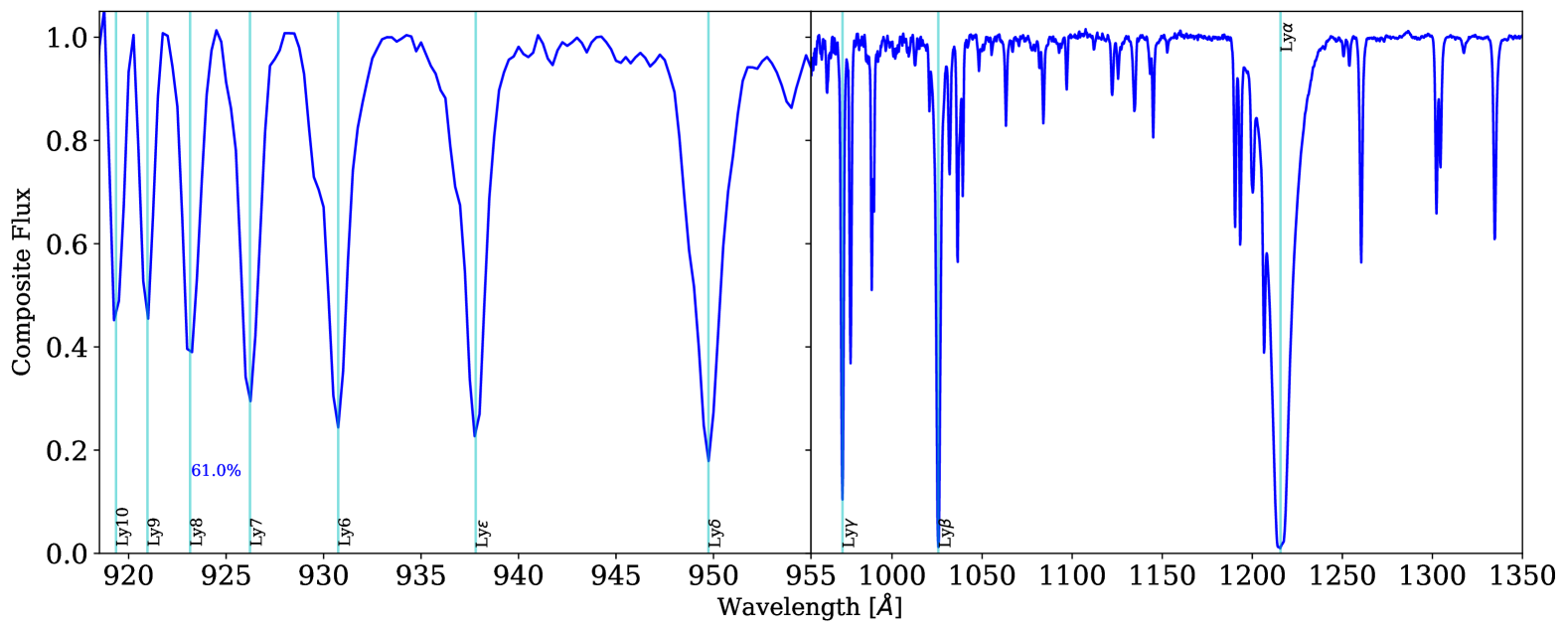
Figure 13: Composite spectrum of DLAs in the DR2 catalog from DLA Toolkit, according to the properties defined in Appendix B. Lyman series lines are marked with vertical cyan lines. The percentage close to the Lyman-8 line represents the purity of the selected DLA sample for DLAs with predicted $z\gtrsim 2.9$.

To explore an alternative approach, we created a combined catalog in which DLA detections from different methods are associated if they fall within 3,000 km s^-1, similar to the threshold used to define true detections in Equation (6). We then applied the same combined catalog definition from Equation (11) to assess the impact of this higher tolerance on purity and completeness.

The resulting purity and completeness, evaluated in the same S/N and $N_{\texttt{HI}}$ bins as in Section IV, are shown in Figure 12. With the increased association tolerance, completeness in all the $\log_{10}(N_{\texttt{HI}})>22.0$ bins improves by approximately 30% when S/N$>2$, while purity decreases by less than 10%. Since high $N_{\texttt{HI}}$ systems are rare, the overall impact on catalog purity and completeness is minimal. The total purity and completeness are now 75.2% and 71.8%, respectively – changing by less than 1% compared to the original catalog – while significantly improving completeness at high $N_{\texttt{HI}}$, which is particularly relevant because these systems compromise a significant fraction of the forest when present.

Appendix B DLA Toolkit DR2 Catalog Composite Spectrum

Calculating purity from a composite spectrum is a tool we can use not only for the combined catalog (see Section VI.1), but for all the DLA finding methods. In this appendix, we tackle the DLAs found by the DLA Toolkit exclusively to understand what data tells us about purity with this method.

We select candidate DLAs with $\Delta\chi_{r}^{2}>0.03$, S/N $>2$, and predicted $\log_{10}(N_{\texttt{HI}})>20.3$ found by the DLA Toolkit in DESI DR2. We additionally remove BAL sightlines, leaving a total of 35,939 candidate DLAs. We then followed the same procedure outlined in Section VI.1. As noted in that section, since the purity is measured using the Lyman-8 flux deficit, we can only assess the purity for the subset of the DLA catalog with predicted $z\gtrsim 2.9$. This corresponds to $\sim$15% (5,498 candidate DLAs) of the DR2 DLA Toolkit catalog after applying the aforementioned quality cuts. As a reminder, the purity measured here can be considered a conservative estimation of purity for the entire sample, owing to the higher forest opacity increasing the frequency of DLA interlopers with higher DLA redshifts.

The stacking result is shown in Figure 13, providing a purity estimate of $61\%$. For comparison, a predicted $z>2.9$ restriction on the mock DLA sample in a purity of $\sim 71$%. An intriguing feature seen in the stack is the non-zero Ly$\alpha$ trough (offset by $\sim 0.025)$, hinting at where the DLA Toolkit may under-perform. Perhaps there are interlopers with similar absorption profiles as DLAs for which the Voigt profile addition in the model reduces the $\chi_{r}^{2}$ sufficiently to constitute a detection. Fortunately, the final combined catalog strategy appears to mitigate much of this type of contamination, as even with the lower purity seen here, the combination of GP, CNN, and DLA Toolkit allows us to retain a significantly high purity.