Heuristic and Optimal Synthesis of CNOT and Clifford Circuits

Abstract

Efficiently implementing Clifford circuits is crucial for quantum error correction and quantum algorithms. Linear reversible circuits, equivalent to circuits composed of CNOT gates, have important applications in classical computing. In this work we present methods for CNOT and general Clifford circuit synthesis which can be used to minimise either the entangling two-qubit gate count or the circuit depth. We present three families of algorithms - optimal synthesis which works on small circuits, A* synthesis for intermediate-size circuits and greedy synthesis for large circuits. We benchmark against existing methods in the literature and show that our approach results in circuits with lower two-qubit gate count than previous methods. The algorithms have been implemented in a GitHub repository for use by the classical and quantum computing community.

1 Introduction

The Clifford group, generated by the single-qubit phase ($S:=\sqrt{Z}$) and Hadamard ($H$) operators, plus the two-qubit controlled-not (CNOT) operator, plays an important part in quantum algorithms and quantum error correction. Examples of Clifford circuits used in the field of quantum error correction include encoding circuits, syndrome extraction circuits and logical gates. Due to the importance of Clifford circuits, finding efficient implementations has been an active area of research. In the classical literature, there is a significant amount of work on synthesis of linear reversible circuits which correspond to Clifford circuits using only CNOT gates [26, 23, 30, 7, 20]. The efficiency of a circuit is usually measured in terms of either the total number of two-qubit entangling gates or the depth of the circuit (the number of time-steps required to implement the circuit). Optimising the gate-count and depth of Clifford circuits is challenging because each Clifford operator has an infinite number of circuit implementations.

In this work, we introduce heuristic (greedy and A*) and optimal algorithms for circuit synthesis. Our algorithms can be applied to either CNOT circuits or general Clifford circuits. We use a mapping from CNOT circuits to invertible binary matrices in $\operatorname{GL}(n,2)$ and from general Clifford operators to symplectic binary matrices in $\operatorname{Sp}(2n,2)$. We consider equivalence classes of circuit matrix representations up to input/output qubit permutations and this results in efficiency gains and lower two-qubit gate counts. In several qubit architectures, qubit permutations can be implemented with low overhead [13, 2, 42, 32] and so we can choose to implement the member of an equivalence class with the lowest two-qubit gate-count or depth. In addition, we can often absorb qubit permutations into the state preparation part of a circuit, even where low-overhead SWAP gates are not available [28, 8].

Our greedy algorithm chooses gates to apply by optimising a vector derived from the column sums of the binary matrix representative of the operator. Existing greedy synthesis algorithms for CNOT circuits optimise a scalar heuristic but tend to become trapped in local minima [30] and our vector-based method is much less susceptible to this issue.

Our optimal synthesis algorithm involves generating a database of matrices by applying all possible two-qubit gates in sequence. Using a variation of the method in [4], we reduce the size of the database by considering equivalence classes of matrices up to row/column permutations, transpose, inverse and, for Clifford circuits, single-qubit Clifford operators applied to the left and right. To synthesise a circuit, we look up the equivalence class in the database and return the saved gate sequence. For optimal CNOT synthesis, we determine the equivalence class of a binary invertible matrix up to row and column permutations by mapping it to a bi-coloured graph using the method in [44] and checking for graph isomorphisms using open source packages such as nauty [18] or Bliss [12, 11]. We show how to extend this method to find equivalence classes of symplectic matrices up to permutations and single-qubit Clifford gates acting on both the left and right. This allows us to generate a significantly smaller database using less computational resources compared to the method in [4].

Our A* synthesis algorithm uses a scalar heuristic $h$ which estimates the number of gates required to reduce the matrix to a permutation matrix (in the case of CNOT circuits) or a permutation combined with a series of single-qubit Clifford operators (for the general symplectic case). The algorithm does not commit to an action immediately, instead saving gate options to a priority queue. By analysing the databases generated in optimal synthesis, we find robust estimators for $h$ based on the row and column sums of matrices. The resulting A* algorithm usually outperforms the greedy algorithm when applied to intermediate circuit sizes.

Benchmarking over a range of circuit sizes, we show that our algorithms have favourable entangling two-qubit gate counts compared to existing methods for both CNOT and general Clifford circuits. Our algorithms have been implemented in a Python package available for use by the community.

2 CNOT Circuit Synthesis

In this section, we consider synthesis of circuits composed entirely of CNOT gates. Circuits of this type have important applications in syndrome extraction and magic state distillation and are also of interest in classical computing applications. The structure of this section is as follows. We first show how to represent any CNOT circuit as an invertible binary matrix such that adding columns of the matrix corresponds to CNOT gates and introduce CNOT synthesis via Gaussian elimination. We then present our three new algorithms for CNOT synthesis. We conclude the section by benchmarking our methods against existing methods, and giving a number of applications.

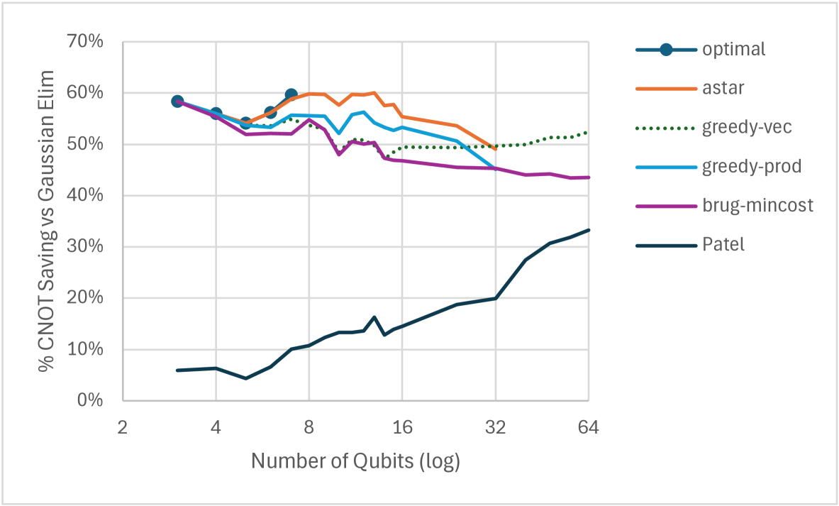
Figure 1: CNOT synthesis algorithm benchmark. Using $400$ randomly generated binary invertible matrices for $3\leq n\leq 64$, we compare our greedy, optimal and A* CNOT synthesis algorithms of Sections˜2.3, 2.4 and 2.5 with the algorithms in [7] (BBVMA) and in [23] (PMH). The CNOT-count of the A* algorithm closely matches optimal gate counts where available and has the lowest CNOT-counts on circuits of up to 32 qubits. For larger circuits, the greedy algorithm with the $\mathbf{h}$ vector heuristic has the lowest CNOT-count.

2.1 Representation of CNOT Circuits as Invertible Binary Matrices

In this section, we show how to represent a CNOT circuit as an invertible binary matrix known as a parity matrix following the material in [20]. For any CNOT circuit, we can find a parity matrix $A$ such that the action of the circuit on a computational basis vector $\ket{\mathbf{e}}$ is given by $\ket{\mathbf{e}A}$. To find the parity matrix, we give $A$ the initial value $I_{n}$ and update $A$ by applying each CNOT gate in sequence. To apply a $\textrm{CNOT}_{ij}$ gate, we add column $i$ of $A$ to column $j$. This is equivalent to multiplying on the right by a binary $n\times n$ matrix which is zero apart from the entry $(i,j)$ and the diagonal entries which are one.

2.2 CNOT Circuit Synthesis via Gaussian Elimination

Synthesis via Gaussian elimination employs the algorithm for determining the parity matrix introduced in Section˜2.1, but operated in reverse. To perform circuit synthesis, we reduce the parity matrix for the desired CNOT circuit to identity via Gaussian elimination by addition of columns (equivalent to a CNOT gate). Applying the gates in reverse order yields a synthesis of the CNOT circuit.

Where the qubit architecture allows SWAP gates to be implemented with low overhead, we can lower the CNOT-count by reducing the parity matrix to a permutation matrix $P$ instead of the identity. Pseudocode for a Gaussian elimination algorithm using this method can be found in Algorithm˜1.

In [23] the authors showed that any CNOT circuit can be implemented by using $O(n^{2}/2\log n)$ CNOT gates. Gaussian elimination gives a circuit using $O(n^{2})$ CNOT gates, and so the algorithm is not asymptotically optimal. We will use Gaussian elimination as our benchmark when comparing algorithms for CNOT synthesis.

2.3 Greedy Synthesis of CNOT Circuits

In this subsection we present our greedy algorithm for CNOT circuit synthesis which has improved CNOT-count compared to Gaussian elimination. The algorithm works by considering all possible CNOT gates at each stage and applying the one which minimises a particular heuristic.

Various greedy CNOT synthesis algorithms have been proposed in previous works and we discuss these here. Synthesis via Gaussian elimination guarantees at each step that at least one entry is eliminated by adding two columns. In practice, we can often eliminate more than one entry if there is a high degree of overlap between two columns. The PMH algorithm of [23] utilises this fact to increase the number of entries eliminated in each column operation. Each column is broken into a series of blocks and any blocks which are equal are added together first. The authors show that the gate-count of the PMH algorithm matches an asymptotically optimal figure of $O(n^{2}/2\log n)$.

There are a number of works using the idea of choosing CNOT gates which eliminate as many entries as possible. In [30, 7] the authors consider algorithms which optimise the selection of CNOT gates by minimising the number of ones in the parity matrix:

$$h_{\text{sum}}(A) :=\left(\sum_{0\leq i,j<n}A_{ij}\right).$$ (1)

In [7], the authors introduce a metric based on the sum of the logarithms of the column sums of the parity matrix. This method gives priority to eliminating entries in columns which are ‘almost done’ and have weight close to 1:

$$h_{\text{prod}}(A) :=\sum_{0\leq j<n}\log\left(\sum_{0\leq i<n}A_{ij}\right).$$ (2)

These works also consider the inverse and transpose of the parity matrix when calculating their heuristics because these can be synthesized using the same number of CNOT gates and may have lower heuristics.

The main drawback of optimising for scalar quantities is that the algorithm tends to get trapped in local minima. The authors of [30] address this by reverting to Gaussian elimination if this occurs.

In [8], MW in collaboration with Nicholas Fazio and Zhenyu Cai, introduced a vector-based heuristic for CNOT circuit synthesis in the context of simplifying magic state distillation circuits. In that method, we reduced the parity matrix to a permutation matrix which corresponds to a qubit permutation. Qubit permutations can be moved to the beginning of the circuit absorbed into state preparation. In this work, we refine the greedy algorithm in that paper and compare it to existing methods in the literature.

We show that our method is less likely to become trapped in local minima versus scalar heuristics. In our comparison, we use scalar heuristics based on those discussed in [30, 7] calculated from combinations of the transpose and inverse of the parity matrix, normalised so that they are zero for a permutation matrix:

$$H_{\text{sum}}(A) :=\left(h_{\text{sum}}(A)+h_{\text{sum}}(A^{-1})\right)/2n-1,$$

$$H_{\text{prod}}(A) :=\left(h_{\text{prod}}(A)+h_{\text{prod}}(A^{T})+h_{\text{prod}}(A^{-1})+h_{\text{prod}}(A^{-T})\right)/4n.$$ (3)

Our vector heuristic is formed by sorting the column sums of the parity matrix, its inverse and its transpose. We first calculate a vector of length $n$ which corresponds to sums of the columns of a matrix $A$. We subtract $1$ from the column sums so that the vector is zero for permutation matrices. The $j$th entry of the column sum vector is given by

$$\text{colSums}(A)[j] :=\sum_{0\leq i<n}A_{ij}-1$$ (4)

The vector heuristic is the result of sorting the length $4n$ vector formed by joining together the column sums of the parity matrix $A$, its transpose $A^{T}$, its inverse $A^{-1}$ and the inverse transpose $A^{-T}$:

$$\mathbf{h}(A) :=\text{sorted}\left[\text{colSums}(A),\text{colSums}(A^{T}),\text{colSums}(A^{-1}),\text{colSums}(A^{-T})\right].$$ (5)

The vector heuristic in [8] includes the column sums of the matrix and its transpose only - we found that including column sums of the inverse and inverse transpose gave better performance in terms of CNOT-count.

We benchmarked our vector heuristic against the $H_{\text{sum}}$ and $H_{\text{prod}}$ scalar heuristics and tracked whether the algorithm became trapped in a local minimum. For each algorithm run, we keep track of the minimum heuristic achieved so far. If the minimum heuristic has not improved after applying 10 gates in a row, we abandon the run on the basis that it has most likely become trapped in a local minimum. Pseudocode for the greedy algorithm is set out in Algorithm˜5 and includes the condition for abandoning the run.

We used a random dataset of 400 CNOT circuits on up to 64 qubits for the benchmark and the results are plotted in Figure˜2. The percentage saving of CNOT-gates versus the Gaussian elimination method of Section˜2.2 is used as our performance benchmark. We found that for all heuristics, the greedy algorithm is unlikely to become trapped in a local minimum for circuits on $n<32$ qubits. In this range, the scalar heuristics $H_{\text{sum}}(A)$ and $H_{\text{prod}}(A)$ gave lower CNOT-counts than the vector heuristic $\mathbf{h}(A)$. For larger circuits, the performance of the scalar heuristics deteriorated, with a $100\%$ abandonment rate for circuits on $n>32$ qubits. For larger circuits, the vector-based heuristic was dominant and gave a 50% reduction in CNOT-count on average versus Gaussian elimination - the data is available on our GitHub repository.

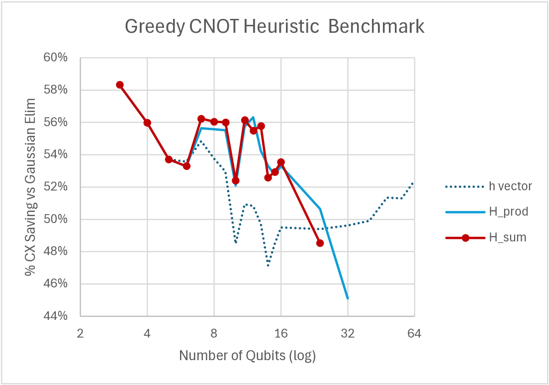
Figure 2: Heuristics for greedy CNOT synthesis. Using $400$ randomly generated binary invertible matrices for $3\leq n\leq 64$, we compare the performance of greedy synthesis using the vector-based heuristic of Equation˜5 to the scalar heuristics of Equation˜3. We find that the scalar heuristics have lower CNOT-count for $n<32$ but for $n\geq 32$ qubits, they tend to get trapped in local minima. The vector-based heuristic continues to perform well for large circuits.

2.3.1 Greedy Depth Optimisation for CNOT Circuits

The methods discussed so far for greedy CNOT synthesis focus on minimising the CNOT count of circuits. In this section, we show how to generalise the greedy algorithm to minimise the depth of the circuit.

Consider an iteration of the greedy algorithm where we consider all possible CNOT gates. In the depth-optimising version of the algorithm, we keep track of the heuristic $\mathbf{h}$ for the previous iteration. For each gate option $G_{i}$, we calculate the depth $d_{i}$ of the resulting circuit. If the heuristic $\mathbf{h}_{i}$ of the new gate is worse than $\mathbf{h}$, we add a large number to $d_{i}$ as a penalty. We then select the CNOT gate which minimises the vector $(d_{i},\mathbf{h}_{i})$, apply the gate $G_{i}$ and update $\mathbf{h}$. Pseudocode for greedy depth optimisation is set out in Algorithm˜5.

2.4 Optimal CNOT Circuit Synthesis

Whilst greedy CNOT synthesis gives good results even for large circuits, it does not guarantee that the CNOT-count will be optimal. In this section we show how to find the minimal number of CNOT gates required for synthesis of CNOT circuits on a small number of qubits ($\leq 7$ qubits) based on the method of [4] for general Clifford circuits. During preparation of this paper, a work using a similar idea for CNOT synthesis has been released using different methods and achieving different results [5]. We generate a database all equivalence classes of $\operatorname{GL}(n,2)$ up to permutations of the rows and columns plus transposes and inverses of matrices. Considering equivalence classes of $\operatorname{GL}(n,2)$ results in an exponential reduction in the database size and processing time. The database is generated in order of the minimum CNOT-count for each class. We also show how to generate the database in order of circuit depth, allowing for synthesis of minimum-depth circuit implementations of CNOT circuits. To synthesize a CNOT circuit, we look up the equivalence class of the parity matrix in the database, then apply a combination of qubit permutations on the left and right of the circuit.

2.4.1 Generating Equivalence Classes of $GL(n,2)$

To generate the matrix database, we start with the $n\times n$ identity matrix, then apply all possible $n(n-1)$ $\textrm{CNOT}_{ij}$ gates to find matrices requiring one CNOT. To find matrices requiring $d+1$ CNOT gates, we start with those requiring $d$ gates and again apply all possible CNOT gates.

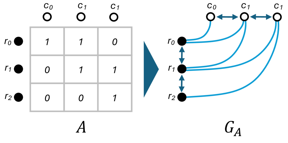
Figure 3: Mapping a binary invertible matrix $A$ to a bi-coloured graph $G_{A}$ using the method of [44]. Each row of the matrix is a vertex of type $r$ and each column a vertex of type $c$ in $G_{A}$. Two vertices $r_{i}$ and $c_{j}$ are joined by an edge in $G_{A}$ if $A_{ij}=1$. Graphs $G_{A}$ and $G_{B}$ are isomorphic if there is a permutation $P_{r}$ of rows and a permutation $P_{c}$ of the columns such that $(r_{i},c_{j})$ is an edge in $G_{B}$ $\iff(P_{r}(r_{i}),P_{c}(c_{j}))$ is an edge in $G_{A}$.

We only add matrices to the database if they are not equivalent to an existing matrix up to permutations of the rows and columns and determining equivalence classes of matrices is the main technical challenge of this approach. This question was addressed in [44] by representing a binary matrix $A$ as a bi-coloured graph $G_{A}$ as set out in Figure˜3. Two binary matrices are in the same equivalence class if and only if their graph representations are isomorphic where labels for vertices of the same type ($r$ or $c$) can be swapped. We use the nauty or Bliss package to test whether graphs are isomorphic [18, 12, 11]. This involves generating a canonical labelling of the graph, which is a permutation of the row and column vertices which puts the graph into a canonical form. We calculate a certificate from the adjacency matrix by converting it into graph6 format string [18]. The certificates for two graphs are equal if and only if the graphs are isomorphic.

Once an invertible matrix has been synthesised, it is straightforward to obtain a synthesis for the transpose, the inverse and the transpose inverse using the same number of CNOT gates. We only add the matrix to the database if the transpose, inverse and inverse transpose have not been generated already. Pseudocode for the database generation algorithm is set out in Algorithm˜7.

We have generated all equivalence classes of invertible binary matrices up to $n=7$ and the results are summarised in Table˜1. We classify the equivalence classes of $GL(n,2)$ by the minimal number of CNOT gates and circuit depth in Tables˜6 and 7. Even with the space savings resulting from considering equivalence classes of matrices, the size of the database grows exponentially with $n$ and it would appear unlikely that generating the database will be practical for $n\geq 9$.

n	$|\operatorname{GL}(n,2)|$	Equiv classes up to col perms	Classes up to row/col perms, transp and inv	Max CNOT-Count	Max Circuit Depth
1	1	1	1	0	0
2	6	3	2	1	1
3	168	28	5	3	3
4	20160	840	27	6	3
5	1.00E+07	8.33E+04	284	8	5
6	2.02E+10	2.80E+07	11,761	12	5
7	1.64E+14	3.251E+10	1.72E+06	14	7

Table 1: Equivalence Classes of Binary Invertible Matrices. In this table, we compare the total number of invertible matrices $|\operatorname{GL}(2,n)|$ with the number of equivalence classes up to row and column permutations, plus transposes and inverses. The database for $n=7$ has $1.7$ million entries and uses around 34MB. The maximum number of CNOT gates required to generate any invertible matrix is noted in the final column.

2.4.2 Optimal Synthesis Algorithm

The optimal synthesis algorithm takes as input an invertible binary matrix $A$. We then construct the bi-coloured graph $G_{A}$ and calculate the graph isomorphism class certificate as explained in Section˜2.4.1. We then search through the database to find a matrix $B$ with the same certificate. Using the canonical labellings of $A$ and $B$, we find row and column permutations $P_{r},P_{c}$ such that $A=P_{r}BP_{c}$. We return the CNOT gates used to generate $B$ conjugated by the permutations $P_{r}$ and $P_{c}$. Finally, the permutation $P_{c}$ is commuted through to the start of the circuit.

2.4.3 Generalisation of Optimal Algorithm to Circuit Depth Optimisation

The algorithm for generating the optimal circuit database can be modified to yield minimum depth circuit implementations. This is done by applying all possible depth-one CNOT circuits at each step, rather than single CNOT gates. Generating all depth-one circuits on $n$ qubits is done by first generating all sets of one or more non-overlapping ordered pairs of qubits $(i,j)$, then applying all possible combinations of $CNOT_{ij}$ and $CNOT_{ji}$ to each pair. We reduce algorithm complexity by only generating depth-one circuits which increase the circuit depth, and the algorithm for generating the sets of non-overlapping pairs of qubits is set out in Algorithm˜4.

2.5 A* Synthesis of CNOT circuits

Optimal synthesis of CNOT circuits via the method in Section˜2.4 is only likely to be possible for up to $n=8$ qubits due to the size of the matrix database. Here we describe an A* algorithm [10] which matches optimal results closely for $n\leq 7$ and can be applied to circuits beyond this range. In the greedy algorithm of Section˜2.3, the gate which minimises the heuristic is applied at each step. In the A* algorithm, gate options are stored as nodes in a priority queue rather than committing to a choice immediately. At each stage, the node with the lowest value of $g(P)+h(P)$ is expanded, where $g(P)$ is the number of CNOT gates applied to reach the matrix $P$ and $h(P)$ is a heuristic which estimates the number of CNOT gates required to reach a permutation matrix from $P$. Providing the heuristic is admissible (i.e. does not over-estimate the true cost to reach the goal), the A* algorithm gives optimal results.

2.5.1 Heuristic for A* Algorithm

The main challenge of the A* method is to choose a suitable heuristic which estimates the number of CNOT gates required to reach a permutation matrix. Using the database generated for $n\leq 7$ for the optimal CNOT synthesis method of Section˜2.4, we found a high correlation between the minimum CNOT-count and the $H_{\text{sum}}$ heuristic of Equation˜3, and a slightly higher correlation with $H_{\text{prod}}$ (Table˜2). Accordingly, we used the heuristics $h=rH_{\text{sum}}(A)$ and $h=rH_{\text{prod}}(P)$ where $r$ is a parameter chosen to be close to the slope $m$ of the line of best fit as calculated in Table˜2. We conducted a sensitivity analysis for both heuristics for a range of values for $r$. The data set used was a random set of 970 invertible $7\times 7$ matrices generated using the method of Section˜2.4. For the $\operatorname{GL}(7,2)$ data set, we found that using the $H_{\text{prod}}$ heuristic gave more robust results and that varying $r$ may be necessary to achieve best results (see Figure˜7).

$H_{\text{sum}}(A)$	n=2	3	4	5	6	7
R	1.00	0.98	0.93	0.90	0.85	0.81
m	2.00	2.22	2.44	2.36	2.25	2.20
b	0.00	0.20	0.71	1.68	3.06	4.62
$H_{\text{prod}}(A)$	n=2	3	4	5	6	7
R	1.00	0.98	0.93	0.91	0.87	0.84
m	2.89	3.60	4.50	5.04	5.64	6.50
b	0.00	0.20	0.52	1.13	1.89	2.53

Table 2: Correlation between CNOT-count and heuristics for invertible $n\times n$ matrix $A$. We first calculate the correlation coefficient $R$, slope $m$ and intercept $b$ of the line of best fit for $H_{\text{sum}}(A)$ which uses the sum of the entries of $A$ and its inverse. We then do the same for $H_{\text{prod}}(A)$ which uses the log of the row and column sums of $A$ and its inverse.

2.5.2 Computational Complexity of A* Algorithm

The main disadvantage of the A* algorithm is that it has exponential worst-case complexity, and the priority queue can become very large. In our A* algorithm we manage the growth of the priority queue as follows. Firstly, we only consider CNOT operations between columns which have some overlap (and hence are likely to reduce the overall weight of the matrix). Secondly, we maintain a maximum queue size at each step using the Treap python implementation of Daniel Stromberg [37]. If the queue exceeds the size limit, we remove the maximal entries. We found that shortening the queue length can reduce the processing time for A* - for instance we use a queue length of 100 for Figure˜1 up to 15 qubits and a queue length of 10 thereafter.

2.5.3 Generalisation of A* Algorithm to Circuit Depth Optimisation

We now show how to generalise the A* algorithm to search for optimal depth circuit implementations. This is done by using a modified $g$ metric. Instead of counting the number of steps the algorithm takes to reach the matrix $P$, we set $g$ to be the depth of the CNOT circuit required to reach $P$. We obtained good results without altering the $h$ metric, though this could be the subject of future work. Pseudocode for the A* algorithm which incorporates an option for depth optimisation is set out in Algorithm˜6.

2.6 CNOT Synthesis Algorithm Benchmark

In this section we compare our greedy, optimal and A* CNOT synthesis algorithms of Sections˜2.3, 2.4 and 2.5 to the BBVMA and PMH algorithms [7, 23]. The dataset used was the same set of 400 randomly generated binary invertible matrices in the range $3\leq n\leq 64$ as in Figure˜2.

We implemented both the BBVMA and PMH algorithms in python and these are available in our GitHub repository [41]. The results of the PMH algorithm matched those in [23] quite closely. The BBVMA algorithm first reduces the parity matrix to a triangular form which is then reduced to the identity. The authors focus mainly on the second step and demonstrate a fast algorithm which has a low CNOT-count. We implemented the pseudocode of Algorithm 1 on page 7 of [7] to reduce a triangular matrix to identity. We implemented a ‘minimising cost’ algorithm for reducing a matrix to triangular form as described on page 13 of [7]. Our method chooses an $(i,j)$ pair at each step which results in the lowest $CNOT$-count or the lowest matrix sum if the $CNOT$-count is equal.

The results of our CNOT synthesis benchmark are in Figure˜1. We found that the CNOT-count of the A* algorithm matched the optimal number up to circuits on up to $n=7$ qubits where optimal data was available. To reduce the run-time of the A* algorithm, we used a relatively maximum low queue size of 100 for $n<16$ and 10 thereafter. We used the scaling heuristic $r=3$. The A* algorithm gave good results for circuits on up to $n=32$.

For circuits on $n\geq 32$ the greedy algorithm with the $\mathbf{h}$ vector heuristic has the lowest CNOT-count by an increasing margin. A spreadsheet collating these results and giving the circuit implementations is available on our GitHub repository.

3 General Clifford Synthesis

In this section, we consider synthesis of general Clifford circuits. Circuits of this type are used in quantum algorithms, in encoding circuits for quantum error correction and in logical gates for quantum codes. In [1] Aaronson and Gottesman show that any Clifford operator has a canonical circuit implementation in 11 layers of the form: $H-\textit{CNOT}-S-\textit{CNOT}-S-\textit{CNOT}-H-S-\textit{CNOT}-S-\textit{CNOT}$. They show that AG synthesis is asymptotically optimal with $O(n^{2}/\log n)$ two-qubit gates. In many cases far more efficient implementations exist, and finding these is the focus of this section. We use AG synthesis as our benchmark for comparing algorithms.

Our approach is to use a circuit structure with only three layers - qubit permutations, single-qubit Cliffords, then 2-qubit symplectic transvections, which are equivalent to CNOT gates up to single qubit Cliffords. This structure allows us to simplify algorithms by considering equivalence classes of operators up to permutations and single-qubit Cliffords acting on either the right or the left hand side of the operator. Transvections are quite natural gates for many quantum architectures, and give us much more freedom to optimise circuits compared to using just CNOT gates [40, 25].

The structure of this section is as follows. We first show how to represent Clifford operators as binary symplectic matrices and introduce symplectic transvections. We then show how to generalise the greedy, optimal and A* algorithms of Sections˜2.3, 2.4 and 2.5 to general Clifford circuits. This unifies the approaches and even allows us to re-use code in many cases. Finally, we benchmark our algorithms against existing methods for Clifford circuit synthesis.

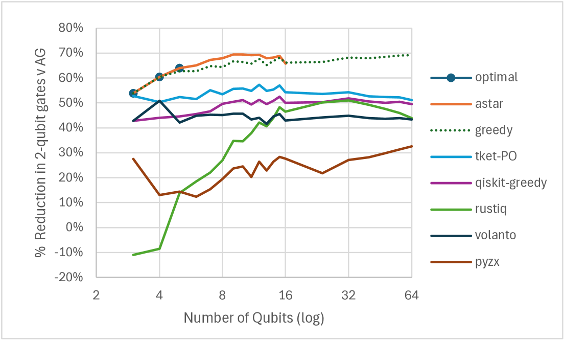
Figure 4: Clifford synthesis algorithm benchmark. We used a dataset of 400 randomly generated symplectic matrices using the method of [38]. The y-axis is the percentage reduction in two qubit gates compared to the Qiskit implementation of AG synthesis [1].

3.1 Binary Symplectic Representation of Clifford Operators

In this subsection, we set out the binary symplectic representation of Clifford operators which will be used in our algorithms. Clifford operators map Paulis to Paulis under conjugation and are defined up to products of Paulis and global phases by specifying the mapping of the Pauli group generators $X_{i}$ and $Z_{i}$ for $0\leq i<n$. We represent Pauli operators as binary strings $(\mathbf{x}|\mathbf{z})$ where $\mathbf{x}$ and $\mathbf{z}$ are length $n$ binary vectors representing the $X$ (resp $Z$) components of the Pauli operator $i^{\mathbf{x}\cdot\mathbf{z}}X(\mathbf{z})Z(\mathbf{z})$ and $X(\mathbf{x}):=\prod_{0\leq i<n}X_{i}^{\mathbf{x}[i]}$.

We represent Clifford operators as $2n\times 2n$ binary symplectic matrices $A$ with four $n\times n$ sub-matrices:

$$A:=\left[\begin{array}[]{c|c}A_{XX}&A_{XZ}\\ \hline\cr A_{ZX}&A_{ZZ}\end{array}\right].$$ (8)

Row $i$ of the matrix $[A_{XX}|A_{XZ}]$ indicates where the Clifford operator maps $X_{i}$ under conjugation. Similarly, row $i$ of $[A_{ZX}|A_{ZZ}]$ (which is row $i+n$ of $A$) gives the mapping of $Z_{i}$. The matrices $A_{XX},A_{ZX}$ are the $X$-components of the mapped Paulis and $A_{XZ},A_{ZZ}$ are the $Z$-components. The Pauli operator represented by row $i$ commutes with all rows of $A$, apart from row $i+n$ with which it anti-commutes (see [1]).

3.2 Symplectic Transvections

For synthesis of general Clifford circuits, we use transvections for our two-qubit gates. Transvections play an important role in symplectic geometry, where it is known that they generate the symplectic group $\text{Sp}(n,2)$ [21], and correspond to geometrical shearing transformations. When the Clifford group is represented using symplectic matrices, certain Clifford group gates can be identified as transvections [16, 27]. A transvection $T_{P}$ on $n$ qubits is defined in terms of a $n$-qubit Pauli operator $P$ as follows:

$$T_{P}:=\exp\left(\frac{i\pi}{4}(I-P)\right).$$ (9)

It can easily be shown that $T_{P}^{2}=P$ so we can think of $T_{P}=\sqrt{P}$. If $P$ has binary representation $\mathbf{v}:=(\mathbf{x}|\mathbf{z})$ then $T_{P}$ has the symplectic representation $I+\Omega\mathbf{v}^{T}\mathbf{v}$ (see Section˜A.2). Two-qubit transvections have support on only two qubits, and are of the form:

$$\sqrt{P_{i}P_{j}}:=T_{P_{i}P_{j}}=\exp\left(\frac{i\pi}{4}(I-P_{i}P_{j})\right),$$ (10)

where $P_{i},P_{j}$ are non-trivial single-qubit Paulis acting on qubits $i,j$ respectively. As there are three non-trivial Paulis on a single qubit, there are $3\times 3=9$ distinct two-qubit transvections.

The Clifford group is generated by two-qubit transvections and single-qubit Cliffords, and we can write the CNOT and CZ operators in terms of transvections as follows:

$$\textrm{CZ}_{ij} =S_{i}^{3}S_{j}^{3}\sqrt{Z_{i}Z_{j}};$$ (11)

$$\textrm{CNOT}_{ij} =S_{i}^{3}\sqrt{X_{j}}^{3}\sqrt{Z_{i}X_{j}}.$$ (12)

Two-qubit transvections are natural gates in a number of qubit architectures, including trapped ions[6], NMR [39], spin qubits and quantum dot systems [19] which further justifies this choice of gate set. Up to a global phase, they are the same as the Pauli product rotations of [17] with angle $\varphi=\pi/4$.

3.3 Greedy Synthesis of Clifford Circuits

We now show how to modify the greedy CNOT synthesis algorithm of Section˜2.3 so that it can be applied to general Clifford circuits. The greedy CNOT circuit algorithm reduces the parity matrix to a permutation matrix. The greedy Clifford algorithm reduces the symplectic matrix for the circuit to a matrix representing a qubit permutation followed by a layer of single-qubit Clifford gates. The termination condition is defined in terms of certain $2\times 2$ sub-matrices of symplectic matrices:

$$F_{ij}:=\left[\begin{array}[]{c|c}A_{i,j}&A_{i,j+n}\\ \hline\cr A_{i+n,j}&A_{i+n,j+n}\end{array}\right].$$

The $F_{ij}$ are either rank 1, rank 2 (invertible) or all zero (rank 0). We keep track of the rank 1 and rank 2 $F_{ij}$ matrices by calculating the matrices $\textit{R1}(A)$ and $\textit{R2}(A)$ respectively as follows:

$$\textit{R1}(A)_{ij} :=\begin{cases}1:\text{ if }\text{Rk}(F_{ij})=1;\\ 0:\text{ otherwise.}\end{cases}$$ (13)

$$\textit{R2}(A)_{ij} :=\begin{cases}1:\text{ if }\text{Rk}(F_{ij})=2;\\ 0:\text{ otherwise.}\end{cases}$$ (14)

The greedy algorithm applies transvections to reduce the symplectic matrix to a form $P$ such that $\textit{R2}(P)$ is a permutation matrix and $\textit{R1}(P)$ is an all-zero matrix. The permutation matrix $\textit{R2}(P)$ corresponds to a qubit permutation, and the rank 2 $F_{ij}$ in $P$ correspond to single-qubit Clifford gates. As $\textit{R2}(P)$ is a permutation matrix, there are $n$ rank 2 $F_{ij}$, with exactly one in each row and column. There are six invertible $2\times 2$ matrices, and these correspond to the symplectic representations of the six single-qubit Cliffords up to Pauli and phase factors. This reduction method was inspired by the synthesis algorithm of Volanto [40], which is analogous to Gaussian elimination for Clifford circuits. We describe a modified Volanto algorithm in Algorithm˜2 which reduces symplectic matrices to the form $P$ described above.

The greedy Clifford synthesis algorithm considers all possible pairs of qubits $(i,j)$ and all nine possible two-qubit transvections at each step. It chooses the option which minimises the vector $\mathbf{h}(A)$ which is defined in a similar way to Equation˜5 using the column sums of R2 and R1 matrices of Equation˜14:

$$\mathbf{h}(A) :=\text{sorted}\left(\text{colSums}(\textit{R2}(A)+\textit{R1}(A)/n),\text{colSums}(\textit{R2}(A^{T})+\textit{R1}(A^{T})/n)\right).$$ (15)

We found that giving a lower weight to the column sums of the R1 matrix gave good results, and in our metric we apply a factor of $n$ as the maxiumum colum sum of an R1 matrix is $n-1$. Because the inverse of a symplectic matrix is given by $A^{-1}=\Omega A^{T}\Omega$, $\textit{R1}(A^{-1})=\textit{R1}(A^{T})$ we do not need to consider the inverse when calculating the heuristic.

3.4 Optimal Clifford Synthesis

We now generalise the method of Section˜2.4 by applying two-qubit symplectic transvections rather than CNOT gates (see Equation˜10). Our method also can be used to perform depth-optimal searches by applying all possible depth one transvection circuits using the qubit partitioning algorithm of Algorithm˜4.

3.4.1 Generating Equivalence Classes of $Sp(n,2)$

We consider equivalence classes of symplectic matrices up to multiplication on the left and right by symplectic matrices corresponding to qubit permutations and a set of single qubit Clifford gates (see Section˜3.3). We have based our method on the one in [4] where the authors show how to calculate a database of optimal circuits for Cliffords on up to 6 qubits. Compared to [4], we generate a significantly smaller number of equivalence classes because we consider permutations of both the input and output qubits, and we also include transpose and inverses of matrices in the same class.

To determine if symplectic matrices are in the same equivalence class, we map to a graph isomorphism problem using a generalisation of the method in Section˜2.4 and this is set out in Figure˜5. We use the nauty [18] or Bliss [12, 11] package to determine if two graphs $G_{A}$ and $G_{B}$ are isomorphic and to generate canonical labellings.

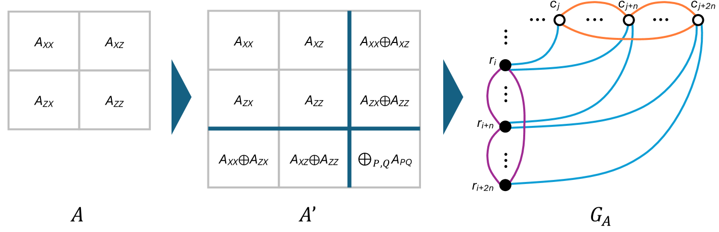
Figure 5: Mapping of symplectic matrices to bi-coloured graphs. We first map the $2n\times 2n$ symplectic matrix $A$ of Section˜3.1 to a $3n\times 3n$ matrix $A^{\prime}$. This is done by adding a third block of rows and columns by summing across the blocks of $A$. There is a vertex of type $r$ in $G_{A}$ for each row of $A^{\prime}$, and a vertex of type $c$ for each column. There is an edge $(r_{i},c_{j})$ in $G_{A}$ if and only if $A^{\prime}_{ij}=1$. We also add the edges $(r_{i},r_{i+n}),(r_{i},r_{i+2n})$ and $(r_{i+n},r_{i+2n})$ for $0\leq i<n$, then do the same for columns. A permutation of the rows which preserves the connectivity of $G_{A}$ can be identified as a combination of SWAP and single-qubit Clifford gates applied on the left (see [4]). Similarly, permutations of columns can be identified as permutations and single-qubit Cliffords applied on the right (see [29]).

In Table˜3, we summarise the number of equivalence classes of symplectic matrices on up to $n=5$ qubits and compare the number of equivalence classes to those calculated in [4]. In Tables˜8 and 9 we classify equivalence classes of symplectic matrices by circuit depth and two-qubit gate count.

n	$|\operatorname{Sp}(n,2)|$	Equiv Classes: This Work	Equiv Classes: Bravyi et al	Max gate count	Max depth
1	6	1	1	0	0
2	720	2	4	2	1
3	1.45E+06	8	27	4	4
4	4.74E+10	109	2,363	6	4
5	2.48E+16	20,421	4,322,659	9	5
6	2.08E+23		1.43E+11

Table 3: Equivalence Classes of Symplectic Matrices. In this table, we compare the total number of binary symplectic matrices $|\operatorname{Sp}(n,2)|$ to the equivalence classes used in our optimal algorithm and those used in [4]. We consider equivalence classes of symplectic matrices up to permutations of both columns and rows and determine equivalence classes by mapping to a graph isomorphism problem using the method of Figure˜5. This significantly reduces the number of equivalence classes and computational complexity versus the method in [4]. The maximum number of two-qubit gates required to generate any invertible matrix and the maximum depth required are noted in the final two columns.

3.4.2 Optimal Synthesis of Clifford Circuits

The algorithm for optimal synthesis of Clifford circuits is as follows. For a given symplectic matrix $A$, we first search the database for a symplectic matrix $B$ with the same graph isomorphism certificate. Using the canonical labelling, we determine a permutation $P_{r}$ on the row vertices and $P_{c}$ on column vertices which sends $G_{B}$ to $G_{A}$. Using the techniques in [29], we map $P_{r}$ and $P_{c}$ to symplectic matrices $S_{r}$ and $S_{c}$ which correspond a combination of single-qubit Cliffords and qubit permutations such that $A=S_{r}BS_{c}$. We return the stored circuit for $B$ prepended by the permutation and single-qubit Cliffords of $S_{r}$ and followed by those of $S_{c}$. The gates of $S_{c}$ are then commuted through to the beginning of the circuit.

3.5 A* Synthesis of Clifford Circuits

We now show how to extend the CNOT A* synthesis algorithm to general Clifford circuits. The key part of the algorithm is to choose a heuristic $h$ for the estimated number of two-qubit transvections required to reduce the symplectic matrix to a qubit permutation followed by a set of single-qubit Cliffords. Our heuristic is based on the number of $F_{ij}$ matrices of various ranks in each row and column of the corresponding symplectic matrix as follows:

$$\textit{R12}(A) :=\textit{R1}(A)+\textit{R2}(A);$$ (16)

$$H_{\text{sum}}(A) :=(h_{\text{sum}}(\textit{R12}(A))+h_{\text{sum}}(\textit{R12}(A^{T})))/2n-1;$$ (17)

$$H_{\text{prod}}(A) :=(h_{\text{prod}}(\textit{R12}(A))+h_{\text{prod}}(\textit{R12}(A^{T})))/2n.$$ (18)

where $h_{\text{sum}}$ and $h_{\text{prod}}$ are as defined in Equation˜3, but applied to the matrix $\textit{R12}(A)$ which indicates which $F_{ij}$ sub-matrices have rank 1 or 2 (see Equation˜14).

Performing a regression analysis on the database of symplectic matrices generated as in Section˜3.4, we find a stronger correlation for $H_{\text{prod}}$ versus $H_{\text{sum}}$. When applied to the dataset of 1003 6-qubit symplectic matrices from [3], we find that $rH_{\text{prod}}(A)$ gives a more robust optimisation which is very close to the known optimal 2-qubit gate count (Figure˜8). We found that the scalar heuristics of Equation˜3 did not perform well for general Clifford synthesis.

$H_{\text{sum}}(A)$	n=2	3	4	5	6
R	1.00	0.95	0.85	0.73	0.50
m	1.00	1.61	1.53	1.69	0.98
b	0.00	-0.10	0.53	0.97	4.89
$H_{\text{prod}}(A)$	n=2	3	4	5	6
R	1.00	0.93	0.85	0.73	0.52
m	1.44	2.98	3.93	6.44	4.84
b	0.00	-0.23	-0.43	-2.69	1.11

Table 4: Correlation between optimal two-qubit gate-count and heuristics for binary symplectic $2n\times 2n$ matrix $A$. The heuristics of Equation˜18 are based on the R12 matrix which tracks which $F_{ij}$ have non-zero rank. We first calculate the correlation coefficient $R$, slope $m$ and intercept $b$ of the line of best fit for $H_{\text{sum}}(\textit{R12}(A))$ which is the sum of all entries in R12. We then do the same for $H_{\text{prod}}(\textit{R12}(A))$ which is the sum of the logs of the row and column sums of R12.

3.6 Clifford Synthesis Algorithm Benchmarks

We benchmarked our greedy, optimal and A* Clifford synthesis algorithms of Sections˜3.3, 3.4 and 3.5 against existing Clifford synthesis algorithms in the literature.

3.6.1 Randomly Generated Cliffords on up to $n=64$ Qubits

We benchmark all methods versus the Qiskit implementation of the Aaronson and Gottesman synthesis algorithm [1] and the results are in Figure 4. The following algorithms were used in the comparison:

• The Qiskit greedy algorithm of [3] is a recursive algorithm which first calculates a circuit to disentangle one of the qubits from the others, then calls the algorithm on the remaining entangled qubits. Note that this method operates quite differently to the greedy algorithm of Section˜3.3.

• The pytket full peephole optimisation of [33] is based on the peephole optimisation method set out in [26] for reversible circuits. Peephole optimisation involves generating a set of known optimal circuits. To optimise a circuit, the algorithm traverses small sections of the circuit and replaces them with an equivalent optimal circuit implementation.

• The rustiq package of [9] implements an graph-state based synthesis algorithm.

• The PyZX package of [14] synthesizes circuits using ZX calculus.

• The modified Volanto algorithm [40] which is described in Algorithm˜2.

We used a dataset of 400 randomly generated symplectic matrices using the method of [38]. The results are summarized in Figure˜4. We found that the A* algorithm matched optimal two-qubit gate counts up to $n=5$, and gave good results for our random dataset up to $n=16$ qubits. To reduce the run-time of the A* algorithm we used a relatively small maximum queue size of 100. We used the heuristic scaling $r=3$ for the A* run. For circuits on $n=16$ qubits, the greedy algorithm gave lower entangling gate counts than the A* algorithm and for $n>16$ qubits, it showed a clear separation against all other methods tested. A spreadsheet collating these results and giving the circuit implementations is available on our GitHub repository.

3.6.2 Hamitonian Dataset on up to $n=64$ Qubits

We then benchmarked using the Hamiltonian dataset of [3] - this is a series of circuits which represent the evolution of a Hamiltonian using various physical qubit layouts. The number of qubits in the circuits varied from 4 to 64. We used only the greedy Clifford synthesis, as optimal synthesis and A* were not possible on the larger circuits. We benchmarked the greedy algorithm versus the BSHM algorithm in [3] followed by one round of the pytket FullPeepholeOptimise pass. This was done to ensure a fair comparison as the BSHM algorithm does not consider permutation equivalence classes of operators, but the pytket algorithm does. We found the greedy algorithm gave better results for both 2-qubit gate count and run time. This was the case for all layouts apart from the cyclic geometries. The results are set out in Figure˜6 and available on our GitHub repository.

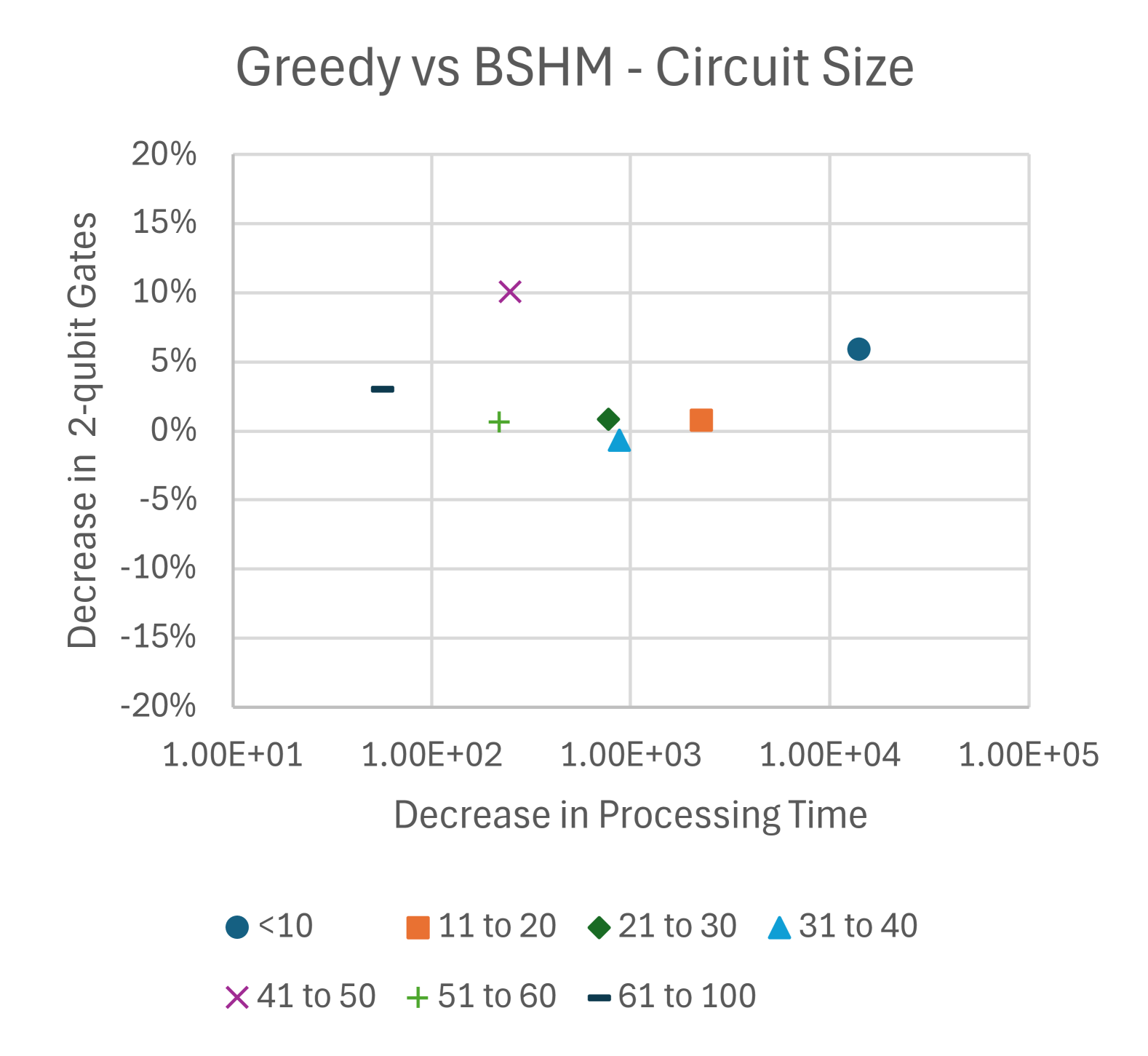
(a) By circuit size

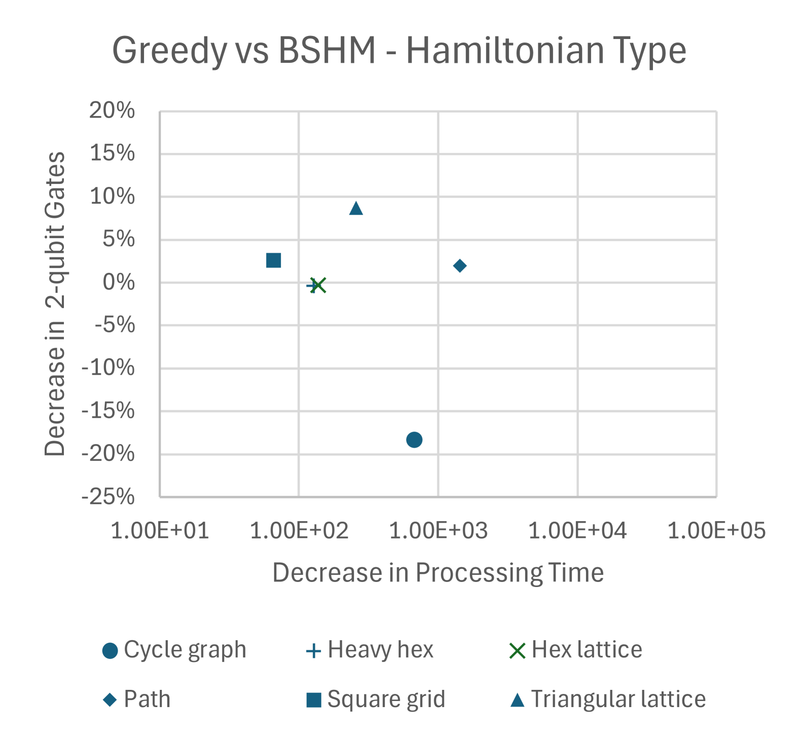
(b) By circuit type

Figure 6: Greedy Clifford synthesis benchmark - Hamiltonian dataset. The charts plot the percentage saving in 2-qubit gatecount and processing time versus the BSHM algorithm of [3].

3.6.3 Encoding Circuits

Encoding circuits are an important class of circuits for Quantum Error Correction. Preparing the logical states $\ket{0}_{L}$ and $\ket{+}_{L}$ is used for instance in Knill [15] and Steane [35] error correction, as well as in quantum algorithms.

In [43] the authors use reinforcement learning to minimize the number of two qubit entangling gates in the $\ket{0}_{L}$ encoding circuit of different codes. They apply their technique on a number of codes, including non-CSS ones such as the perfect $[[5,1,3]]$ code. They also apply it to larger codes, such as the Golay $[[23,1,7]]$ code [34], where they find a $\ket{0}_{L}$ encoding circuit with $61$ entangling two qubit gates. In [22], however, the authors found a circuit using $57$ CNOT gates, by adapting Steane’s Latin Rectangle method [36] to minimize overlaps. Using our A* method, we found an encoding circuit using $56$ entangling two qubit gates, improving the best-known result. The results and comparisons are shown in Table 5.

Furthermore, in [24, 31] Boolean satisfiability solving techniques are leveraged to obtain optimal logical state preparation circuits for a number of CSS codes in terms of entangling gate count. Applying the A* algorithm to the same codes gave circuits which match the optimal entangling gate counts. The greedy method gave results very close to optimal.

The results and comparisons for logical state synthesis can be found in our GitHub repository.

Code	RLFQC	A*	Greedy	Pytket	Qiskit	Volanto	PyZX	Rustiq
$[[5,1,3]]$ Perfect Code	6	6	6	7	8	7	10	12
$[[7,1,3]]$ Steane Code	8	8	8	10	11	12	9	22
$[[9,1,3]]$ Shor Code	8	8	8	10	10	11	9	11
$[[15,1,3]]$ Reed-Muller	22	22	22	31	32	37	24	55
$[[17,1,5]]$ Colour Code	37	31	33	43	43	42	42	52
$[[19,1,5]]$ Colour Code	49	45	49	61	61	70	67	151
$[[23,1,7]]$ Golay Code	61	56	69	96	97	118	138	237
$[[25,1,5]]$ Surface Code	54	54	53	72	72	61	71	84
TOTAL	245	230	248	330	334	358	370	624

Table 5: Entangling two qubit gate count in $\ket{0}_{L}$ encoding circuit for the codes in [43]. We compare the reinforcement learning method of [43] to our greedy and A* algorithms, as well as various other circuit optimisation algorithms.

4 Conclusion and Open Questions

In this work, we have set out algorithms for synthesis of CNOT and general Clifford circuits which have lower two-qubit gate count than existing methods, and can also be applied to optimise for circuit depth.

The optimal synthesis algorithms can be used for CNOT circuits on $n\leq 7$ qubits and Clifford circuits on $n\leq 5$ qubits. By using the optimised coding techniques of [4] it may well be possible to extend this size range. Determining a closed expression for the maximum circuit depth and two-qubit gate-count to reach any desired CNOT or Clifford circuit would be an interesting question to address.

The A* synthesis algorithms closely matches optimal 2-qubit gate counts where these are available, and can be used for intermediate-size circuits. The algorithm has exponential run time in the worst case, but this can be managed by shortening the maximum priority queue length. Using the data from optimal synthesis, we could use more sophisticated machine learning methods to determine the heuristic $h$ and this has potential to improve the accuracy of the method.

The greedy algorithm out-performs existing methods for larger circuit sizes. The output of the greedy algorithm could be used as input to pattern-matching algorithms such as [3, 33].

We have implemented our algorithms in python to enable rapid development and maximal re-use of code between the algorithms. The speed of the algorithms could be improved by porting them to C or Rust, allowing them to be used effectively on larger circuits. The algorithms could also be modified to take into account the gate set and connectivity of particular devices, though we have not built this functionality.

These algorithms have been made available to the classical and quantum computing communities in our GitHub repository [41].

5 Acknowledgments

MW and DEB are supported by the Engineering and Physical Sciences Research Council [grant number EP/W032635/1 and EP/S005021/1]. SK and DEB are supported by the Engineering and Physical Sciences Research Council [grant number EP/Y004620/1 and EP/T001062/1]. The authors acknowledge the use of the UCL Kathleen High Performance Computing Facility (Kathleen@UCL), and associated support services, in the completion of this work. The authors would like to thank Hasan Sayginel, Nicholas Fazio and Zhenyu Cai for helpful discussions.

Appendix A Algorithm Pseudocode

In this appendix, we present pseudocode for the algorithms used in this paper. We start by describing Gaussian elimination and Volanto synthesis for CNOT and general Clifford circuits respectively, highlighting their similarities. We then introduce our greedy algorithm with its modifications to allow for early termination when trapped in local minima and optimisation of circuit depth rather than gate-count. Finally, we describe the A* algorithm and the closely related optimal synthesis algorithm.

A.1 Modified Gaussian Elimination

We first present a modified version of Gaussian elimination which can be used for CNOT circuit synthesis. The modified algorithm has the following variations to the usual one. Firstly, it scans down rows and across columns to perform eliminations via column operations. Secondly, it reduces invertible matrices to a permutation matrix $P$ rather than to identity. To assist with this, it maintains a set pOptions of unused pivots. The output of the algorithm is the permutation matrix P plus a set of CNOT gates opList which when applied to P give A.

Algorithm 1 Modified Gaussian Elimination

Input:

A: a $n\times n$ binary invertible matrix

Output:

P: a permutation matrix; AND

opList: series of CNOT gates yielding A when applied to P; OR

FALSE: if A is not invertible

Method:

opList := [], pOptions := [0..n-1], P := copy(A)

for i in [0..n-1] do$\triangleright$ i is the current row

  R := [p for p in pOptions if P[i,p]=1] $\triangleright$ unused pivots which are non-zero in row i

  if len(R)=0 then

   return FALSE$\triangleright$ the matrix is not full rank

  end if

  p := R.removeMin() $\triangleright$ remove smallest element of R, save as p

  pOptions.remove(p) $\triangleright$ remove p from unused pivots

  for j in R do

   op:= (CNOT,(p,j))

   applyOp(P,op), opList.append(op)

  end for

end for

return P, inverse(opList)

A.2 Symplectic Representation of Transvections

In this section, we find the symplectic matrix representation of the transvections defined in Equation˜9.

Proposition

Let $T_{P}:=\exp\left(\frac{i\pi}{4}(I-P)\right)$ where $P$ is a Pauli with binary representation $\mathbf{v}$ satisfying $P^{2}=I$. $T_{P}$ has symplectic representation $I+\Omega\mathbf{v}^{T}\mathbf{v}$

Proof

Define the projectors $A_{\pm}:=\frac{1}{2}(I\pm P)$. Note that $A_{\pm}^{2}=A_{\pm}$ and $I=A_{+}+A_{-}$. Let $A_{-}(\theta):=\exp\left({i\theta}A_{-}\right)$ so that $T_{P}=A_{-}(\frac{\pi}{2})$. Expanding $A_{-}(\theta)$, we have:

$$A_{-}(\theta) :=\exp\left({i\theta}A_{-}\right)$$

$$=I+\frac{i\theta}{1!}A_{-}-\frac{\theta^{2}}{2!}A_{-}-i\frac{\theta^{3}}{3!}A_{-}+\frac{\theta^{4}}{4!}A_{-}+...$$

$$=A_{+}+A_{-}(\cos\theta+i\sin\theta)$$

Setting $\theta:=\frac{\pi}{2}$ and $\theta:=\pi$:

$$T_{P} =A_{-}\left(\frac{\pi}{2}\right)=A_{+}+iA_{-},$$

$$T_{P}^{2} =A_{-}(\pi)=A_{+}-A_{-}=\frac{1}{2}(I+P-(I-P))=P.$$

Since $P^{2}=I$, $T_{P}T_{P}^{3}=I$ and so $T_{P}^{-1}=PT_{P}$. Now consider the action of $T_{P}$ on a Pauli operator $Q$ under conjugation. If $P$ and $Q$ commute then:

$$T_{P}QT_{P}^{-1} =T_{P}T_{P}^{-1}Q=Q.$$

Otherwise, if $P$ and $Q$ anti-commute:

$$T_{P}QT_{P}^{-1} =(A_{+}+iA_{-})QP(A_{+}+iA_{-})$$

$$=-(A_{+}+iA_{-})P(A_{-}+iA_{+})Q$$

$$=-\frac{1}{i}(A_{+}+iA_{-})(A_{+}-iA_{-})PQ$$

$$=i(A_{+}+A_{-})PQ=iPQ.$$

We claim the symplectic matrix $I+\Omega\mathbf{v}^{T}\mathbf{v}$ has the same action acting by right matrix multiplication on vector representations of Paulis. Let $Q$ have vector representation $\mathbf{u}$. The expression $\mathbf{u}\Omega\mathbf{v}^{T}$ is the symplectic inner product and is zero if $Q$ commutes with $P$ and 1 otherwise. If $P$ and $Q$ commute then $\mathbf{u}(I+\Omega\mathbf{v}^{T}\mathbf{v})=\mathbf{u}+(\mathbf{u}\Omega\mathbf{v}^{T})\mathbf{v}=\mathbf{u}$ and so $Q$ is mapped to itself. If $P$ and $Q$ anti-commute then $\mathbf{u}(I+\Omega\mathbf{v}^{T}\mathbf{v})=\mathbf{u}+(\mathbf{u}\Omega\mathbf{v}^{T})\mathbf{v}=\mathbf{u}+\mathbf{v}$. Because addition of vector representations corresponds to multiplication of Paulis up to $\pm 1$, $Q$ is mapped to $PQ$ up to a global phase.

A.3 Modified Volanto Synthesis Algorithm

In this section, we present a modified version of Volanto Clifford synthesis (see [40]). The algorithm works by reducing the symplectic matrix representation of a Clifford circuit to a matrix which represents a qubit permutation followed by a series of single-qubit Clifford gates (see Section˜3.3). The modified Volanto algorithm works by scanning down the rows of the matrix. For each row, it ensures that there is exactly one $F_{ij}$ matrix of rank $2$ and none of rank $1$ (see Section˜3.3). The algorithm does this by reducing pairs of rank $2$ $F_{ij}$ in the row to rank $1$, then reduces the remaining rank $1$ $F_{ij}$ to all-zero matrices.

In the tableau view of symplectic matrices [1], $F_{ij}$ represents a pair of single-qubit Paulis acting on qubit $j$ - one of which is part of a stabiliser in row $i$ and one of which is an anti-commuting destabiliser in row $i+n$. It can easily be verified that single-qubit Paulis acting on qubit $j$ anti-commute if and only if $F_{ij}$ is of rank $2$. Hence there are always an odd number of full-rank $F_{ij}$ in any row $i$ or column $j$.

To eliminate pairs $F_{ij},F_{ik}$ in row $i$ which are both of rank $2$, we apply the transvection $\textit{T2}_{ijk}:=\sqrt{i^{ac+bd}X_{j}^{a}Z_{j}^{b}X_{k}^{c}Z_{k}^{d}}$ on the right where $(a,b)$ is the first row of $F_{ij}$ and $(c,d)$ is the second row of $F_{ik}$. Given that there is an odd number of $F_{ij}$ of rank 2 in each row, this leaves a single $F_{ij}$ of rank 2 in the row and we use column $j$ as the pivot for row $i$.

We eliminate $F_{ik}$ of rank 1 as follows. The pivot matrix $F_{ij}$ is of rank 2 so it is invertible by assumption. As $F_{ik}$ of rank 1, $F_{ij}^{-1}F_{jk}=\begin{bmatrix}b\\ a\end{bmatrix}\begin{bmatrix}c&d\end{bmatrix}$ where $a(b):=1$ if the second (first) row of $F_{ij}^{-1}F_{jk}$ is non-zero and $c(d):=1$ if the first (second) column is non-zero. Applying the transvection $\textit{T1}_{ijk}:=\sqrt{i^{ac+bd}X_{j}^{a}Z_{j}^{b}X_{k}^{c}Z_{k}^{d}}$ on the right reduces $F_{ik}$ to the all-zero matrix.

The result of the algorithm is a symplectic matrix which has exactly one matrix $F_{ij}$ of rank 2 for each row $i$ and column $j$, and no matrices of rank $1$. This can be interpreted as a qubit permutation which is defined by the pivot for each row followed by a series of single-qubit Clifford gates. The modified algorithm returns the single qubit Clifford gates, a qubit permutation and the reversed list of 2-qubit transvections.

Note the similarities to the modified Gaussian elimination algorithm of Algorithm˜1. In particular it maintains a list of unused pivots and returns FALSE if A is not symplectic.

Algorithm 2 Modified Volanto Synthesis

Input:

A: a $2n\times 2n$ binary symplectic matrix

Output:

P: the final reduced matrix; AND

opList: series of 2-qubit transvections yielding A when applied to P; OR

FALSE: if A is not symplectic

Method:

opList := [], pOptions := [0..n-1], P := copy(A)

for i in [0..n-1] do$\triangleright$ i is the current row

  R := [p for p in pOptions if Rank(F(P,i,p) = 2] $\triangleright$ unused pivots with Rank($F_{ip}$)=2

  if len(R) mod 2 = 0 then

   return FALSE$\triangleright$ symplectic matrices have an odd number of $F_{ip}$ of rank 2

  end if

  p := R.removeMin() $\triangleright$ remove smallest element of R, save as p

  pOptions.remove(p) $\triangleright$ remove p from unused pivots

  for a in [0..len(R)/2 - 1] do

   j:=R[2a], k:=R[2a+1]

   op := (T2(P,i,j,k),(j,k)) $\triangleright$ T2 on qubits $(j,k)$ reduces $F_{ij},F_{ik}$ to rank 1

   applyOp(P,op), opList.append(op)

  end for

  R := [j for j in [0..n-1] if Rank(F(P,i,j) = 1]

  for j in R do

   op := (T1(P,i,p,j),(i,j)) $\triangleright$ T1 on qubits $(i,j)$ reduces $F_{ij}$ to zero

   applyOp(P,op), opList.append(op)

  end for

end for

return P, opList

A.4 Algorithms for Optimising Circuit Depth

Our algorithms can be used to either optimise for entangling 2-qubit gate count or circuit depth. We now describe two important helper functions to facilitate depth optimisation. The first is a function for determining the depth of a circuit. Circuits are stored as lists of ordered pairs (opType,qList where opType is a string describing the gate type and qList is a list of qubit indices to which the gate is applied:

Algorithm 3 depth(opList)

Input:

opList: a list of gates

Output:

d: depth of the circuit corresponding to opList.

Method:

layers := []

for (opType,qList) in opList do

  if opType not in [‘QPerm’,‘SWAP’] and len(qList) > 1 then

   L:=len(layers), i := L

   while i > 0 and (qList $\cap$ layers[i-1]) != $\emptyset$ do

     i := i - 1

   end while

   if i = L then:

     layers.append(qList)

   else

     layers[i] := layers[i] + qList

   end if

  end if

end for

return len(layers)

We now describe an algorithm which is used to find all circuits of depth one for a particular 2-qubit gate set. The QPart function is a recursive function returns all combinations of non-overlapping pairs of qubits from a set of qubit indices S which increase the depth of the circuit. It takes as input the support Supp of the previous layer of gates.

Algorithm 4 QPart(S, Supp)

Input:

S: a list of qubit indices

Output:

pList: list of all possible sets of non-overlapping ordered pairs with elements from S

Method:

pList := [[]], LS = len(S)

for i in [0..LS-2] do

  for j in [i+1..LS-1] do

   p := (i,j)

   if p $\cap$ Supp != $\emptyset$ then

     S1 = [S[k] for k in ([i+1..j-1,j+1..LS-1])]

     pList := pList + [([p] + pList1) for pList1 in Q2part(S1)])

   end if

  end for

end for

return pList

A.5 Greedy Synthesis Algorithm

We next set out a greedy algorithm which generates a circuit using a scalar or vector heuristic (see Equations˜3 and 5). The algorithm can either be run for invertible matrices or symplectic matrices. By setting minDepth := TRUE, the user can optimise for minimum depth rather than minimum 2-qubit gate-count. The algorithm terminates if maxWait gates have been applied without reducing the optimisation heuristic, allowing us to track whether the algorithm has become trapped in a local minimum. The function applyOp(A,op) applies a two-qubit gate to the binary symplectic matrix A.

Algorithm 5 Greedy Synthesis

Input:

A: a $2n\times 2n$ binary symplectic matrix

gateOpts: a function returning 2-qubit gate options which can be applied to a matrix

Heuristic: a heuristic function which is zero if the matrix is in the desired final form

minDepth: TRUE to find minimize depth or FALSE to minimize 2-qubit gate count.

maxWait: max iterations to try improving the heuristic before exiting;

Output:

P: reduced matrix; AND

opList: series of 2-qubit operators yielding A when applied to P; OR

FALSE: if maxWait exceeded

Method:

opList := [], P:= copy(A)

hLast := Heuristic(P), hMin := hLast

currWait := 0

while hLast != 0 do

  dhMin:=None$\triangleright$ find gate which minimises depth and heuristic

  for op in GateOpts(A) do

   B := applyOp(P,op)

   hB := Heuristic(B)

   dB := 0

   if minDepth then

     dB := depth(opList + [op])

     if hB > hLast then

      dB := dB + 10000$\triangleright$ penalise gates which do not improve heuristic

     end if

   end if

   if dhMin is None or dhMin > (dB,hB) then

     dhMin := (dB,hB), opMin := op

   end if

  end for

  dLast, hLast := dhMin$\triangleright$ update hLast, P and opList

  P := applyOp(P,opMin)

  opList.append(opMin)

  if hMin > hLast then

   hMin := hLast, currWait := 0 $\triangleright$ better than hMin - reset currWait

  else

   currWait := currWait+1$\triangleright$ hLast worse than hMin - increment currWait

  end if

  if currWait > maxWait then$\triangleright$ exit if maxWait gates since heuristic improved

   return False

  end if

end while

return inverse(opList), P

A.6 A* Synthesis Algorithm

Here we set out the A* synthesis algorithm of Sections˜2.5 and 3.5. The A* algorithm takes one of the heuristics of Equation˜3 as input. The algorithm can either be run for invertible matrices or symplectic matrices. By setting minDepth := TRUE, the user can optimise for minimum depth rather than minimum 2-qubit gate-count. The GateOpts function gives the possible gates which can be applied to the matrix at each step. The size of the priority queue is limited to the input maxQ - we use the treap data structure and removeMax function to manage the queue length. We also maintain a tree database in TreeDB. Each row represents a matrix and stores only the parent ID plus the gate required to reach the corresponding matrix to reduce memory overhead. We use the function TreeDB.retrieve(AId) to retrieve matrix representation and the gate list of the row indexed by AId.

Algorithm 6 A* Synthesis

Input:

A: a $2n\times 2n$ binary symplectic matrix

gateOpts: a function returning 2-qubit gate options which can be applied to a matrix

Heuristic: a heuristic function which is zero if the matrix is in the desired final form

minDepth: TRUE to find minimize depth or FALSE to minimize 2-qubit gate count.

maxQ: maximum size of the priority queue.

Output:

B: the final reduced matrix; AND

opList: series of 2-qubit operators yielding A when applied to B

Method:

B := copy(A),AId :=-1,BId:=0,op:= None,gB:=0,hB:=Heuristic(B)

visited:=[B]

TreeDB := [(AId,op)]$\triangleright$ parent and gate.

PriQ := new treap()

PriQ.append((gB+hB,gB,BId)) $\triangleright$ Insert item with priority gB+hB to priority queue

while len(todo) > 0 do

  ghA,gA,AId := PriQ.removeMin()

  A, opListA:=TreeDB.retrieve(AId)

  for op in GateOpts(A) do

   B := applyOp(A,op)

   if B not in visited then

     hB := Heuristic(B), BId := BId + 1

     TreeDB.append((AId,op))

     if hB = 0 then

      return B, opListA + [op]

     end if

     gB := depth(opListA + [op]) if minDepth else gA+1

     PriQ.append((gB+hB,gB,BId)), visited.append(B)

   end if

  end for

  while len(PriQ) > maxQ do$\triangleright$ remove excess items from PriQ

   PriQ.removeMax()

  end while

end while

return FALSE

A.7 Sensitivity Analysis for A*

Here we present results on optimising the heuristic $h$ for the A* algorithm. We consider both changing the parameter $r$ and swapping between the $H_{\text{sum}}$ and $H_{\text{prod}}$ metrics of Equation˜3.

For the CNOT circuit case, a sensitivity analysis performed on the $\operatorname{GL}(7,2)$ dataset for the different cost function heuristics gives us the following results in Figure 7, with data available online.

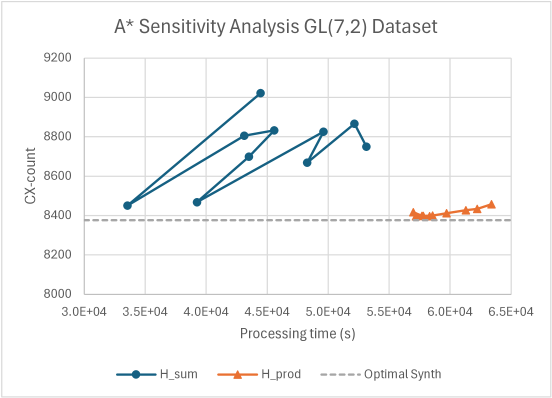
Figure 7: Sensitivity analysis for CNOT A* synthesis algorithm. The blue line represents A* using the matrix weight heuristic $H_{\text{sum}}(A)$ for values of $r$ in the range 2.0-3.0. The orange line uses the log of col and row sums heuristic $H_{\text{prod}}(A)$ for $r$ in the range 1.5-2.4. We plot the total CNOT-count for the data set of 970 elements of $\operatorname{GL}(7,2)$ versus the total time taken. We see that $H_{\text{prod}}(A)$ heuristic gives results closer to the known optimal CNOT-count of 8376 for the data set.

Similarly for the Clifford circuit synthesis, using the $6$ qubit Clifford circuit dataset of [3], we obtain the below results in Figure 8, with data available online.

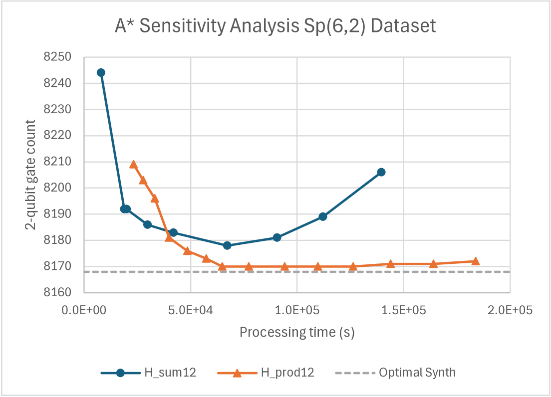
Figure 8: Sensitivity analysis for Clifford A* synthesis algorithm. The blue line represents A* using the matrix weight heuristic $rH_{\text{sum}}(A)$ for values of $r$ in the range 1.65-2.05. The orange line uses the log of col and row sums heuristic $rH_{\text{prod}}(A)$ for $r$ in the range 3.7-5.0. We plot the total two-qubit gate-count for the data set from [3] of 1003 elements of $\operatorname{Sp}(6,2)$ versus the total time taken. We see that $H_{\text{prod}}(A)$ heuristic gives results closer to the best-known gate-count of 8168 for the data set.

A.8 Generating a Database of Matrix Equivalence Classes

We now set out the algorithm for generating a database of equivalence classes of matrices in $\operatorname{GL}(n,2)$ or $\operatorname{Sp}(n,2)$. As in the A* algorithm, we save only the tree structure of the database and retrieve the gate list and matrix using the TreeDB.retrieve(AId) function. Gate options are calculated using the GateOpts function. For optimal depth synthesis, GateOpts returns the set of all depth-one circuits calculated using the method of Algorithm˜4. Otherwise, GateOpts returns the set of all two-qubit gate options - for CNOT synthesis these are all possible CNOT gates on $n$ qubits, whereas for Clifford synthesis it is the set of all two-qubit transvections (see Section˜3.2). The function Canonize(B) generates the graph corresponding to B and returns the certificate for the equivalence class.

Algorithm 7 Optimal Database Generation

Input:

n: number of qubits

gateOpts: function giving possible gates which can be applied to a matrix. For optimal depth mode, these are depth-one circuits.

Canonize: function giving canonical graph isomorphism certificate for a matrix.

Output:

TreeDB: A database where each row corresponds to an equivalence class of matrices and gives the parent node and the operation required to generate the matrix.

Method:

B:=I(2n)

BCert:=Canonize(B)

visited:=[BCert]$\triangleright$ list of visited equivalence classes

AId:=None, op:=None$\triangleright$ No parent or operation for identity matrix

TreeDB:=[(AId,op,0,0)]$\triangleright$ Tree database - store parent and operation in a list

BId := 0$\triangleright$ pointer to last row of TreeDB

SId := 0$\triangleright$ pointer to first row of current iteration

while BId >= SId do

  SId := BId + 1

  for AId in [SId..BId] do$\triangleright$ iterate through newly added rows of TreeDB

   A,opListA:= TreeDB.retrieve(AId)

   for inv in [0,1] do

     for transp in [0,1] do $\triangleright$ apply gates to $A,A^{-1},A^{T},A^{-T}$

      for op in GateOpts(A) do$\triangleright$ apply all possible gates

        B:=applyOp(A,op)

        BInv:=Inverse(B)

        BCert := min([Canonize(Bi) for Bi in [B, B.T, BInv, BInv.T]])

        if BCert not in visited then

         TreeDB.append((AId, op, transp, inv))$\triangleright$ add new row to TreeDB

         visited.append(BCert)$\triangleright$ update visited

         BId := BId + 1$\triangleright$ increment BId

        end if

      end for

     end for

     A:=Transpose(A)

   end for

   A:=Inverse(A)

  end for

end while

return TreeDB

Appendix B Equivalence Classes of Matrices by Gate-Count and Circuit Depth

Here we include supplementary data on the equivalence classes of invertible and symplectic matrices grouped by minimum gate-count and circuit depth.

In Tables˜6 and 7 we list the equivalence classes of $GL(n,2)$ by CNOT count and circuit depth as generated by the optimal CNOT synthesis algorithm of Section˜2.4.

CNOT Count	n=2	3	4	5	6	7
0	1	1	1	1	1	1
1	1	1	1	1	1	1
2		2	3	3	3	3
3		1	8	10	11	11
4			10	40	52	54
5			3	87	257	308
6			1	106	1,123	2,228
7				32	3,235	14,733
8				4	4,698	78,679
9					2,167	291,836
10					209	625,945
11					3	571,160
12					1	132,375
13						2,172
14						2
Total	2	5	27	284	11,761	1,719,491

Table 6: Classification of $\operatorname{GL}(n,2)$ matrix equivalence classes by minimum CNOT-count.

Depth	n=2	3	4	5	6	7
0	1	1	1	1	1	1
1	1	1	2	2	3	3
2		2	9	17	47	91
3		1	14	139	1,805	15,861
4			1	124	9,687	866,885
5				1	218
6
7
Total	2	5	27	284	11,761	1,719,491

Table 7: Classification of $\operatorname{GL}(n,2)$ matrix equivalence classes by minimum circuit depth.

In Tables˜8 and 9 we list the equivalence classes of $Sp(n,2)$ by 2-qubit gate count and circuit depth as generated by the optimal Clifford synthesis algorithm of Section˜3.4. We have calculated these up to $n=5$, and have partial results for $n=6$.

Tv Count	n=2	3	4	5	6
0	1	1	1	1	1
1	1	1	1	1	1
2		2	3	3	3
3		3	11	13	14
4		1	37	78	89
5			47	530	823
6			9	3,325	10,502
7				10,317	142,847
8				6,125	1,767,694
9				28	14,875,711
10
11
12
Total	2	8	109	20,421

Table 8: Classification of $\operatorname{Sp}(n,2)$ matrix equivalence classes by minimum number of 2-qubit gate-count.

Depth	n=2	3	4	5	6
0	1	1	1	1	1
1	1	1	2	2	3
2		2	11	19	54
3		3	84	958	2,071
4		1	11	16,385	62,731
5				3,056
6
7
Total	2	8	109	20,421

Table 9: Classification of $\operatorname{Sp}(n,2)$ matrix equivalence classes by circuit depth.

References

- Aaronson and Gottesman [2004] Scott Aaronson and Daniel Gottesman. Improved simulation of stabilizer circuits. Physical Review A, 70(5):052328, November 2004. ISSN 1050-2947, 1094-1622. doi: 10.1103/PhysRevA.70.052328. arXiv:quant-ph/0406196.
- Baart et al. [2015] Timothy A. Baart et al. Single-spin CCD. Nature nanotechnology, 11 4:330–4, 2015. doi: 10.1038/nnano.2015.291. URL https://api.semanticscholar.org/CorpusID:29106558.
- Bravyi et al. [2021] Sergey Bravyi, Ruslan Shaydulin, Shaohan Hu, and Dmitri Maslov. Clifford circuit optimization with templates and symbolic Pauli gates. Quantum, 5:580, November 2021. ISSN 2521-327X. doi: 10.22331/q-2021-11-16-580. arXiv:2105.02291 [quant-ph].
- Bravyi et al. [2022] Sergey Bravyi, Joseph A. Latone, and Dmitri Maslov. 6-qubit optimal Clifford circuits. npj Quantum Information, 8(1):79, July 2022. ISSN 2056-6387. doi: 10.1038/s41534-022-00583-7. arXiv:2012.06074 [quant-ph].
- Christensen et al. [2025] Jens Emil Christensen, Søren Fuglede Jørgensen, Andreas Pavlogiannis, and Jaco van de Pol. On exact sizes of minimal CNOT circuits, 2025. URL https://arxiv.org/abs/2503.01467.
- Cirac and Zoller [1995] J. I. Cirac and P. Zoller. Quantum computations with cold trapped ions. Phys. Rev. Lett., 74:4091–4094, May 1995. doi: 10.1103/PhysRevLett.74.4091. URL https://link.aps.org/doi/10.1103/PhysRevLett.74.4091.
- De Brugière et al. [2021] Timothée Goubault De Brugière et al. Gaussian elimination versus greedy methods for the synthesis of linear reversible circuits. ACM Transactions on Quantum Computing, 2(3), September 2021. doi: 10.1145/3474226. URL 10.1145/3474226.
- Fazio et al. [2025] Nicholas Fazio, Mark Webster, and Zhenyu Cai. Low-overhead magic state circuits with transversal CNOTs, 2025. URL https://arxiv.org/abs/2501.10291.
- Goubault de Brugière et al. [2025] Timothée Goubault de Brugière, Simon Martiel, and Christophe Vuillot. A graph-state based synthesis framework for Clifford isometries. Quantum, 9:1589, January 2025. ISSN 2521-327X. doi: 10.22331/q-2025-01-14-1589.
- Hart et al. [1968] Peter E. Hart, Nils J. Nilsson, and Bertram Raphael. A formal basis for the heuristic determination of minimum cost paths. IEEE Transactions on Systems Science and Cybernetics, 4(2):100–107, 1968. doi: 10.1109/TSSC.1968.300136.
- Junttila and Kaski [2007] Tommi Junttila and Petteri Kaski. Engineering an efficient canonical labeling tool for large and sparse graphs. In David Applegate et al., editors, Proceedings of the Ninth Workshop on Algorithm Engineering and Experiments and the Fourth Workshop on Analytic Algorithms and Combinatorics, pages 135–149. SIAM, 2007. doi: 10.1137/1.9781611972870.13.
- Junttila and Kaski [2011] Tommi Junttila and Petteri Kaski. Conflict propagation and component recursion for canonical labeling. In Alberto Marchetti-Spaccamela and Michael Segal, editors, Theory and Practice of Algorithms in (Computer) Systems – First International ICST Conference, TAPAS 2011, Rome, Italy, April 18–20, 2011. Proceedings, volume 6595 of Lecture Notes in Computer Science, pages 151–162. Springer, 2011. doi: 10.1007/978-3-642-19754-3\_16.
- Kielpinski et al. [2002] David Kielpinski, C.R. Monroe, and D.J. Wineland. Architecture for a large-scale ion-trap quantum computer. Nature, 417:709–11, 07 2002. doi: 10.1038/nature00784.
- Kissinger and van de Wetering [2020] Aleks Kissinger and John van de Wetering. PyZX: Large scale automated diagrammatic reasoning. Electronic Proceedings in Theoretical Computer Science, 318:229–241, May 2020. ISSN 2075-2180. doi: 10.4204/eptcs.318.14. URL http://dx.doi.org/10.4204/EPTCS.318.14.
- Knill [2005] E. Knill. Quantum computing with realistically noisy devices. Nature, 434(7029):39–44, March 2005. ISSN 1476-4687. doi: 10.1038/nature03350. URL https://doi.org/10.1038/nature03350.
- Koenig and Smolin [2014] Robert Koenig and John A. Smolin. How to efficiently select an arbitrary Clifford group element. Journal of Mathematical Physics, 55(12):122202, December 2014. ISSN 0022-2488, 1089-7658. doi: 10.1063/1.4903507. arXiv:1406.2170 [quant-ph].
- Litinski [2019] Daniel Litinski. A game of surface codes: Large-scale quantum computing with lattice surgery. Quantum, 3:128, March 2019. ISSN 2521-327X. doi: 10.22331/q-2019-03-05-128. URL http://dx.doi.org/10.22331/q-2019-03-05-128.
- McKay and Piperno [2014] Brendan D. McKay and Adolfo Piperno. Practical graph isomorphism, ii. Journal of Symbolic Computation, 60:94–112, 2014. ISSN 0747-7171. doi: 10.1016/j.jsc.2013.09.003. URL https://www.sciencedirect.com/science/article/pii/S0747717113001193.
- Meunier et al. [2011] Tristan Meunier, Victor E. Calado, and Lieven M. K. Vandersypen. Efficient controlled-phase gate for single-spin qubits in quantum dots. Phys. Rev. B, 83:121403, Mar 2011. doi: 10.1103/PhysRevB.83.121403. URL https://link.aps.org/doi/10.1103/PhysRevB.83.121403.
- Murphy and Kissinger [2023] Ewan Murphy and Aleks Kissinger. Global synthesis of CNOT circuits with holes. Electronic Proceedings in Theoretical Computer Science, 384:75–88, August 2023. ISSN 2075-2180. doi: 10.4204/EPTCS.384.5. arXiv:2308.16496 [quant-ph].
- O’Meara [1978] O.T. O’Meara. Symplectic Groups. Mathematical Surveys and Monographs. American Mathematical Society, 1978. ISBN 9780821815168. URL https://books.google.co.uk/books?id=BWHyBwAAQBAJ.
- Paetznick and Reichardt [2012] Adam Paetznick and Ben W. Reichardt. Fault-tolerant ancilla preparation and noise threshold lower boudds for the 23-qubit golay code. Quantum Info. Comput., 12(11–12):1034–1080, November 2012. ISSN 1533-7146.
- Patel et al. [2008] K.N. Patel, I.L. Markov, and J.P. Hayes. Optimal synthesis of linear reversible circuits. Quantum Information and Computation, 8(3 & 4):282–294, March 2008. ISSN 15337146, 15337146. doi: 10.26421/QIC8.3-4-4.
- Peham et al. [2024] Tom Peham, Ludwig Schmid, Lucas Berent, Markus Müller, and Robert Wille. Automated synthesis of fault-tolerant state preparation circuits for quantum error correction codes, 2024. URL https://arxiv.org/abs/2408.11894.
- Pllaha et al. [2021] Tefjol Pllaha, Kalle Volanto, and Olav Tirkkonen. Decomposition of Clifford gates. In 2021 IEEE Global Communications Conference (GLOBECOM), page 01–06, December 2021. doi: 10.1109/GLOBECOM46510.2021.9685501. URL http://arxiv.org/abs/2102.11380. arXiv:2102.11380 [quant-ph].
- Prasad et al. [2006] Aditya K. Prasad, Vivek V. Shende, Igor L. Markov, John P. Hayes, and Ketan N. Patel. Data structures and algorithms for simplifying reversible circuits. J. Emerg. Technol. Comput. Syst., 2(4):277–293, October 2006. ISSN 1550-4832. doi: 10.1145/1216396.1216399.
- Rengaswamy et al. [2018] Narayanan Rengaswamy, Robert Calderbank, Henry D. Pfister, and Swanand Kadhe. Synthesis of logical Clifford operators via symplectic geometry. In 2018 IEEE International Symposium on Information Theory (ISIT), page 791–795, Vail, CO, USA, June 2018. IEEE. ISBN 978-1-5386-4781-3. doi: 10.1109/ISIT.2018.8437652. URL https://ieeexplore.ieee.org/document/8437652/.
- Rodriguez et al. [2024] Pedro Sales Rodriguez, John M. Robinson, Paul Niklas Jepsen, et al. Experimental demonstration of logical magic state distillation, 2024. URL https://arxiv.org/abs/2412.15165.
- Sayginel et al. [2024] Hasan Sayginel, Stergios Koutsioumpas, Mark Webster, Abhishek Rajput, and Dan E Browne. Fault-tolerant logical Clifford gates from code automorphisms, 2024. URL https://arxiv.org/abs/2409.18175.
- Schaeffer and Perkowski [2014] Ben Schaeffer and Marek Perkowski. A cost minimization approach to synthesis of linear reversible circuits, 2014. URL https://arxiv.org/abs/1407.0070.
- Schmid et al. [2025] Ludwig Schmid, Tom Peham, Lucas Berent, Markus Müller, and Robert Wille. Deterministic fault-tolerant state preparation for near-term quantum error correction: Automatic synthesis using boolean satisfiability, 2025. URL https://arxiv.org/abs/2501.05527.
- Simmons [2024] Stephanie Simmons. Scalable fault-tolerant quantum technologies with silicon color centers. PRX Quantum, 5:010102, Mar 2024. doi: 10.1103/PRXQuantum.5.010102. URL https://link.aps.org/doi/10.1103/PRXQuantum.5.010102.
- Sivarajah et al. [2020] Seyon Sivarajah et al. t|ket⟩: a retargetable compiler for NISQ devices. Quantum Science and Technology, 6(1):014003, nov 2020. doi: 10.1088/2058-9565/ab8e92. URL https://dx.doi.org/10.1088/2058-9565/ab8e92.
- Steane [1996] A. M. Steane. Simple quantum error-correcting codes. Phys. Rev. A, 54:4741–4751, Dec 1996. doi: 10.1103/PhysRevA.54.4741. URL https://link.aps.org/doi/10.1103/PhysRevA.54.4741.
- Steane [1997] A. M. Steane. Active stabilization, quantum computation, and quantum state synthesis. Phys. Rev. Lett., 78:2252–2255, Mar 1997. doi: 10.1103/PhysRevLett.78.2252. URL https://link.aps.org/doi/10.1103/PhysRevLett.78.2252.
- Steane [2004] Andrew M. Steane. Fast fault-tolerant filtering of quantum codewords, 2004. URL https://arxiv.org/abs/quant-ph/0202036.
- [37] Daniel R Stromberg. treap: Python implementation of treaps. URL http://stromberg.dnsalias.org/˜dstromberg/treap/.
- Van Den Berg [2021] Ewout Van Den Berg. A simple method for sampling random Clifford operators. In 2021 IEEE International Conference on Quantum Computing and Engineering (QCE), pages 54–59, 2021. doi: 10.1109/QCE52317.2021.00021.
- Vandersypen and Chuang [2005] Lieven M. K. Vandersypen and Isaac L. Chuang. NMR techniques for quantum control and computation. Rev. Mod. Phys., 76:1037–1069, Jan 2005. doi: 10.1103/RevModPhys.76.1037. URL https://link.aps.org/doi/10.1103/RevModPhys.76.1037.
- Volanto [2023] Kalle Volanto. Minimizing the number of two-qubit gates in Clifford circuits. Master’s thesis, Aalto University, March 2023.
- [41] Mark Webster. CliffordOpt: Optimisation of Clifford Circuits. URL https://github.com/m-webster/CliffordOpt.
- Xiao et al. [2024] Yang Xiao et al. Effective nonadiabatic holonomic swap gate with Rydberg atoms using invariant-based reverse engineering. Phys. Rev. A, 109:062610, Jun 2024. doi: 10.1103/PhysRevA.109.062610. URL https://link.aps.org/doi/10.1103/PhysRevA.109.062610.
- Zen et al. [2024] Remmy Zen, Jan Olle, Luis Colmenarez, Matteo Puviani, Markus Müller, and Florian Marquardt. Quantum circuit discovery for fault-tolerant logical state preparation with reinforcement learning, 2024. URL https://arxiv.org/abs/2402.17761.
- Živković [2006] Miodrag Živković. Classification of small (0,1) matrices. Linear Algebra and its Applications, 414(1):310–346, 2006. ISSN 0024-3795. doi: 10.1016/j.laa.2005.10.010. URL https://www.sciencedirect.com/science/article/pii/S0024379505004933.