Advances in Local Analytic Sector Subtraction: massive NLO and elements of NNLO automation

Abstract

In this article we present a number of developments within the scheme of Local Analytic Sector Subtraction for infrared divergences in QCD. First, we extend the scheme to deal with next-to-leading-order (NLO) singularities related to massive QCD particles in the final state. Then, we document a new implementation of the NLO subtraction scheme in the MadNkLO automated numerical framework, which is constructed to host higher-order subtraction algorithms. In particular, we discuss improvements in its performances with respect to the original implementation. Finally we describe the MadNkLO implementation of the first elements relevant to Local Analytic Sector Subtraction at next-to-next-to-leading order (NNLO), in the case of massless QCD partons in the final state.

1 Introduction

The quest for a deeper understanding of fundamental particle interactions and the identification of potential new phenomena at colliders crucially rely on the availability of high-accuracy theoretical predictions for complex scattering processes.

As the accuracy required for the modern precision-physics collider programme well exceeds the leading-order approximation in the Standard Model perturbation theory, computations inevitably have to deal with the presence of infrared (IR) divergences. These arise in separate contributions to scattering cross sections, and are guaranteed to cancel Kinoshita:1962ur ; Lee:1964is when such contributions are properly combined for the prediction of physical observables.

The problem of IR divergences at next-to-leading order (NLO) in QCD perturbation theory was solved in full generality already in the late ‘90s Frixione:1995ms ; Frixione:1997np ; Catani:1996jh ; Catani:1996vz ; Nagy:2003qn by means of IR subtraction. Within this method, the universal long-distance behaviour of scattering amplitudes is leveraged to design functions, the so-called IR counterterms, which approximate real-radiation squared matrix elements in all of their IR-singular limits. The difference between matrix elements and counterterms is then by construction integrable point by point in the phase space, and lends itself to a stable numerical evaluation. On the other hand, the counterterms, subtracted from real-radiation matrix elements, are analytically integrated in the radiation phase space, and then added back to virtual loop contributions, ensuring in turn their IR finiteness. The availability of numerical frameworks automating NLO IR subtraction schemes Campbell:1999ah ; Gleisberg:2007md ; Frederix:2008hu ; Czakon:2009ss ; Hasegawa:2009tx ; Frederix:2009yq ; Alioli:2010xd crucially spurred a theoretical accuracy revolution in the early 2000s, which has been instrumental for the success of the precision-physics programme of the first runs of the Large Hadron Collider (LHC).

At next-to-NLO (NNLO) in QCD, IR subtraction is a very active field of research. On one side, NNLO accuracy is required nowadays for a wider and wider class of processes, to cope with the LHC precision needs. On the other hand, the complexity of the IR problem increases significantly with respect to the NLO case, owing to the much more involved structure of matrix elements and of their IR divergences. Several viable NNLO subtraction schemes have been formulated Frixione:2004is ; GehrmannDeRidder:2005cm ; Currie:2013vh ; Somogyi:2005xz ; Somogyi:2006da ; Somogyi:2006db ; Czakon:2010td ; Czakon:2011ve ; Anastasiou:2003gr ; Caola:2017dug ; Catani:2007vq ; Grazzini:2017mhc ; Boughezal:2011jf ; Boughezal:2015dva ; Boughezal:2015aha ; Gaunt:2015pea ; Cacciari:2015jma ; Sborlini:2016hat ; Herzog:2018ily ; Magnea:2018hab ; Magnea:2018ebr ; Capatti:2019ypt ; TorresBobadilla:2020ekr in the last two decades. This has progressively extended the scope of NNLO QCD results, nowadays reaching processes with five external light particles at Born level (see for instance Kallweit:2020gcp ; Chawdhry:2021hkp ; Czakon:2021mjy ; Badger:2023mgf ), and even allowing the first differential predictions at next-to-NNLO (N³LO) in QCD for simple processes Dreyer:2016oyx ; Dreyer:2018qbw ; Currie:2018fgr ; Chen:2021isd ; Chen:2021vtu ; Billis:2021ecs ; Camarda:2021ict ; Chen:2022cgv ; Chen:2022lwc . Nevertheless, a fully general solution of the NNLO subtraction problem has not been reached yet, with plenty of room for improvement in the universality and versatility of the subtraction algorithms.

The method of Local Analytic Sector Subtraction Magnea:2018hab ; Magnea:2020trj ; Bertolotti:2022ohq ; Bertolotti:2022aih was designed to minimise the complexity of IR counterterms, and especially of their analytic integration over the radiative phase space. In Magnea:2018hab the features of the method were introduced, while the main elements for analytic integration at NNLO were laid down in Magnea:2020trj , for the case of massless QCD in the final state. In Bertolotti:2022aih , such features enabled the first analytic proof of the cancellation of NNLO IR singularities for generic processes with massless QCD particles in the final state. In Bertolotti:2022ohq the case of QCD in the initial state was considered at NLO, and the first implementation of the subtraction scheme was presented in the MadNkLO automated framework Lionetti:2018gko ; Hirschi:2019fkz ; Becchetti:2020wof .

The present article builds on the ingredients of Bertolotti:2022ohq ; Bertolotti:2022aih , presenting developments in different directions within the environment of Local Analytic Sector Subtraction. First, in Section 2, we consider the subtraction of singularities due to QCD radiation from massive final-state particles at NLO. After defining and analytically integrating the relevant counterterms, we show how the resulting poles organise to match the known virtual one-loop singularities in presence of massive particles. Appendices A–C collect several technical details related to the analytic integration of massive counterterms. In particular, different parametrisations of the massive phase space are studied, with the aim of providing ingredients that will allow the integration of massive counterterms at NNLO, which is left for a future development. In Section 3 we document a new implementation of the Local Analytic Sector Subtraction scheme in the automated MadNkLO framework. New features have been introduced to overcome the technical limitations of the original implementation of Bertolotti:2022ohq , especially concerning numerical phase-space integration and execution time. We show a validation of this new implementation at NLO in Section 3.1, both for processes with massless and with massive QCD particles in the final state. MadNkLO is constructed to streamline the generation of all the universal ingredients entering the computation of scattering cross sections at higher perturbative orders. In Section 3.2 we report the MadNkLO implementation of the first elements for Local Analytic Sector Subtraction at NNLO, in the case of massless final-state QCD particles. In particular, we focus on finiteness tests relevant to a production channel in the $e^{+}e^{-}\to jj$ process at NNLO. Some details on NNLO subtraction are collected in Appendix D. Finally, Section 4 contains conclusions and future perspectives.

We note that the Local Analytic Sector Subtraction scheme for massless final-state radiation at NNLO is also being implemented independently of MadNkLO, in the numerical framework Chargeishvili:2024ggm ; Chargeishvili:2024xuc ; Kardos:2024guf , where all NNLO final-state analytic integrals of Magnea:2020trj were also independently verified.

2 NLO subtraction with massive particles

In Bertolotti:2022ohq the NLO Local Analytic Sector Subtraction for massless QCD partons in the final as well as in the initial state was described in detail. In this section we extend the NLO subtraction procedure to the case of massive QCD particles in the final state.

In general, an NLO QCD real squared matrix element $R$ is singular when the extra radiated parton with respect to Born level, labelled with $i$, is a soft gluon, namely it has vanishing energy, $k_{i}^{0}\to 0$. We denote with ${\bf S}_{i}$ the operation of singling out such a soft configuration. Moreover, if $R$ features at least two massless QCD partons $i$ and $j$, it develops a collinear singularity whenever their relative angle $\theta_{ij}$ approaches 0. The corresponding operator extracting this limit is denoted with ${\bf C}_{ij}$.

We will discuss in detail these two types of configurations in the next subsections, after introducing phase-space partitions to disentangle different singular regions.

2.1 Phase-space partitions and counterterm definition

We handle the presence of multiple singular regions in the real matrix elements by introducing partition (or sector) functions $\mathcal{Z}_{ij}$ Frixione:1995ms ; Bertolotti:2022aih for each pair $ij$ of massless QCD partons. Since sector functions are determined uniquely by massless partons, the presence of massive particles in the final state does not prevent us from using the same definitions as in Bertolotti:2022aih for partitions. Setting $q^{\mu}$ as the total momentum of the initial state, and $s_{qa}=2\,q\cdot k_{a}$, with $k_{a}$ the momentum of particle $a$, we thus define sectors as

$$\mathcal{Z}_{ij}\,\equiv\,\frac{\sigma_{ij}+\sigma_{ji}}{\sum\limits_{k}\sum\limits_{l<k}(\sigma_{kl}+\sigma_{lk})}\,,\qquad\quad\sigma_{ab}\,\equiv\,\theta_{{a}\in{\rm F}}\,\theta_{{b\,}\in{\rm F}\!,{\rm I}}\,\frac{s_{qb}}{s_{ab}}\,,\qquad\quad\sum\limits_{i}\sum\limits_{j<i}\mathcal{Z}_{ij}\,=\,1\,,$$ (1)

where $s_{ab}=2\,k_{a}\cdot k_{b}$, and the sums run over all massless QCD partons present in the considered scattering process at real-emission level. We stress that $\mathcal{Z}_{ij}$ is symmetric under label exchange. The symbol $\theta_{\cal C}$ is $1$ ($0$) if condition $\cal C$ is (is not) fulfilled, so that

$$\theta_{{a}\in{\rm M}}\,\equiv\,\mbox{$a$ is a massive particle in the final state,}$$

$$\theta_{{a}\in{\rm F}}\,\,(\theta_{{a}\in{\rm I}})\,\equiv\,\mbox{$a$ is a massless particle in the final (initial) state,}$$

and $\theta_{a\,\in{\rm X,Y}}\equiv\theta_{a\,\in{\rm X}}+\theta_{a\,\in{\rm Y}}$, for $\rm X,Y=F,M,I$.

By construction, when acting with singular soft or collinear limits on a given sector function $\mathcal{Z}_{ij}$, only ${\bf S}_{i}$, ${\bf S}_{j}$, and ${\bf C}_{ij}$ return a non-vanishing result. In other words, a partition $\mathcal{Z}_{ij}$ is built to dampen all singularities of the real matrix element except the mentioned ones, together with their composite soft-collinear configurations. The action of singular limits on $\mathcal{Z}_{ij}$ yields

$${\bf S}_{i}\,\mathcal{Z}_{ij}\,=\,\frac{\sigma_{ij}}{\sum\limits_{k\neq i}\sigma_{ik}}\,,\qquad\sum_{j\neq i}\,{\bf S}_{i}\,\mathcal{Z}_{ij}=1\,,\qquad{\bf C}_{ij}\,\mathcal{Z}_{ij}\,=\,1\,,\qquad{\bf S}_{i}\,{\bf C}_{ij}\,\mathcal{Z}_{ij}\,=\,1\,.\qquad$$ (2)

In each phase-space sector $\mathcal{Z}_{ij}$ the structure of real-radiation singularities is trivial, as it stems uniquely from at most one collinear and two soft singularities. This makes it straightforward to define an infrared counterterm relevant for partition $\mathcal{Z}_{ij}$ as

$$K_{ij} \equiv \Big{[}\,\overline{\bf S}_{i}+\overline{\bf S}_{j}+\overline{\bf C}_{ij}\big{(}1-\overline{\bf S}_{i}-\overline{\bf S}_{j}\big{)}\Big{]}\,R\,\mathcal{Z}_{ij}$$ (3)

$$\equiv \Big{[}\,\overline{\bf S}_{i}+\overline{\bf S}_{j}+\overline{\bf HC}_{ij}\Big{]}\,R\,\mathcal{Z}_{ij}\,.$$

We highlight that the notation ($\overline{\bf S}_{i}$, $\overline{\bf S}_{j}$, and $\overline{\bf C}_{ij}$) used in Eq. (3) for soft and collinear counterterms differs by means of a bar from the one (${\bf S}_{i}$, ${\bf S}_{j}$, and ${\bf C}_{ij}$) used for the corresponding strict limit operations. As will be detailed in the next subsections, barred limits acting on $R$ differ from unbarred ones only by subleading-power terms. The latter guarantee counterterm kinematics to be on shell and Born momentum conserving for all radiative configurations. For this reason we also refer to the barred limits defining the counterterm as improved limits. At variance with the case of matrix elements, the action of improved limits on NLO sector functions is defined to be identical to that of unimproved limits, i.e. $\overline{\bf L}\,\mathcal{Z}_{ij}={\bf L}\,\mathcal{Z}_{ij}$, for all soft, collinear, or soft-collinear limits $\bf L$. Moreover, in Eq. (3), for any improved limit $\overline{\bf L}$, it is understood that $\overline{\bf L}\,R\,\mathcal{Z}_{ij}=(\overline{\bf L}\,R)\,(\overline{\bf L}\,\mathcal{Z}_{ij})=(\overline{\bf L}\,R)\,({\bf L}\,\mathcal{Z}_{ij})$. Finally, the notation $\overline{\bf HC}$ indicates a singular collinear configuration with all of its soft singularities subtracted off, namely a hard-collinear improved limit.

The subtracted real radiation is then given by

$$R^{\,\rm sub}_{ij}\,\equiv\,R\,\mathcal{Z}_{ij}-K_{ij}\,,\qquad\quad R^{\,\rm sub}\,\equiv\,\sum_{i}\sum_{j<i}\,R^{\,\rm sub}_{ij}\,=\,R-K\,,$$ (4)

where $R^{\,\rm sub}_{ij}$ and, in turn, $R^{\,\rm sub}$ are free of non-integrable singularities over the whole radiative phase space. The counterterm $K$ is defined as

$$K\,\equiv\,\sum_{i}\sum_{j<i}\,K_{ij}\,=\,\sum_{i}\,\theta_{{i}\in{\rm F}}\,\overline{\bf S}_{i}\,R+\sum_{i}\sum_{j<i}\,\theta_{{i}\in{\rm F}}\,\theta_{{j}\in{\rm F}\!,{\rm I}}\,\overline{\bf HC}_{ij}\,R\,,$$ (5)

where in the latter step we have used the sum rules in Eq. (2) to get rid of partition functions. The counterterm is a collection of soft and hard-collinear improved limits acting on the real matrix element $R$, to be integrated in the radiative phase space to match the explicit poles of the virtual matrix element $V$.

We note that the counterterm outlined in Eq. (5) is structurally identical to the one relevant to the fully massless case (see for instance Eq. (2.31) of Bertolotti:2022aih ). Physics-wise, its differences are only due to the fact that a soft gluon can now correlate massive colour sources, while a collinear splitting may involve the momentum of a massive particle in its parametrisation. In the following sections we define such massive soft and hard-collinear counterterms, and perform their analytic integration over the radiative phase space.

2.2 Soft counterterm with massive particles

The soft limit ${\bf S}_{i}$ of the real matrix element $R$ is

$${\bf S}_{i}\,R\,=\,-\,\mathcal{N}_{1}\sum_{k\neq i}\sum_{l\neq i}\,\mathcal{I}_{kl}^{(i)}\,B_{kl}(\{k\}_{\not{i}})\,,\qquad\qquad\mathcal{I}_{kl}^{(i)}\,=\,\theta_{{i}\in{\rm F}}\,f_{i}^{g}\,\frac{s_{kl}}{s_{ik}\,s_{il}}\,,$$ (6)

where in the eikonal kernel $\mathcal{I}_{kl}^{(i)}$ the symbols $\theta_{{i}\in{\rm F}}\,f_{i}^{g}$ specify that the contribution is null in QCD unless the soft parton is a final-state gluon. In particular, $f_{a}^{x}$ is meant as a Kronecker symbol prescribing the flavour of $a$ to be equal to $x$, with $x=q,\bar{q},g$.

Indices $k$ and $l$ in Eq. (6) run over all initial-state and final-state, massless as well as massive QCD particles. The soft limit of QCD amplitudes is independent of the mass of the colour source, however mass effects appear at the squared-amplitude level, where the diagonal terms $\mathcal{I}^{(i)}_{aa}$, proportional to $s_{aa}=2\,m_{a}^{2}$, are non vanishing only for massive radiators. The soft kinematics $\{k\}_{\not}{i}$ represents the set of real-radiation momenta after removal of soft momentum $k_{i}^{\mu}$. The colour-correlated Born matrix element is schematically defined as

$$B_{kl}\,=\,\langle{\mathcal{A}}_{n}^{(0)}|{\bf T}_{k}\cdot{\bf T}_{l}|{\mathcal{A}}_{n}^{(0)}\rangle\,,$$ (7)

where $|{\mathcal{A}}_{n}^{(0)}\rangle$ is the Born amplitude written as a ket in colour space Catani:1996vz , undergoing non-trivial transformations under the action of the SU($N_{c}$) generators ${\bf T}_{a}$. Lastly, the normalisation coefficient $\mathcal{N}_{1}$ reads

$$\mathcal{N}_{1}\,=\,8\pi\alpha_{s}\left(\frac{\mu^{2}e^{\gamma_{E}}}{4\pi}\right)^{\epsilon}\,,$$ (8)

with $\alpha_{s}$ the strong coupling, $\mu$ the renormalisation scale, $\epsilon=2-d/2$ the dimensional regulator, and $\gamma_{E}\sim 0.57721$ the Euler-Mascheroni constant.

Exploiting colour algebra, together with the symmetry of the eikonal and of the colour-connected Born under exchange of indices, the soft limit in Eq. (6) can be equivalently rewritten as

$${\bf S}_{i}\,R\,=\,-\,2\,\mathcal{N}_{1}\sum_{k\neq i}\sum_{\begin{subarray}{c}l\neq i\\ l<k\end{subarray}}\mathcal{E}_{kl}^{(i)}\,B_{kl}(\{k\}_{\not{i}})\,,\qquad\qquad\mathcal{E}_{kl}^{(i)}\,\equiv\,\mathcal{I}_{kl}^{(i)}-\frac{1}{2}\mathcal{I}_{kk}^{(i)}-\frac{1}{2}\mathcal{I}_{ll}^{(i)}\,.$$ (9)

In order to construct the corresponding counterterm $\overline{\bf S}_{i}\,R$, we introduce massive dipole mappings Catani:2002hc of real-radiation momenta $\{k\}$ onto Born-level ones $\{\bar{k}\}$. Given three momenta $k_{a}$, $k_{b}$, $k_{c}$, with $k_{a}^{2}=0$, the mappings are defined as

$$\{k\}\,\to\,\{\bar{k}\}^{(abc)}\,\equiv\,\Big{\{}\{k\}_{\not{a}\not{b}\not{c}},\bar{k}_{b}^{(abc)},\bar{k}_{c}^{(abc)}\Big{\}}\,,$$ (10)

so that the Born momenta $\bar{k}_{b}^{(abc)}\equiv\bar{k}_{b}$ and $\bar{k}_{c}^{(abc)}\equiv\bar{k}_{c}$ satisfy mass-shell conditions $\bar{k}_{b}^{2}=m_{b}^{2}$, $\bar{k}_{c}^{2}=m_{c}^{2}$, as well as Born momentum conservation at each point of the real-emission phase space $\Phi_{{n+1}}$. The soft counterterm is then given by

$$\overline{\bf S}_{i}\,R \equiv \overline{\bf S}_{i}^{(0)}R+\overline{\bf S}_{i}^{({\rm M})}R\,,$$ (11)

where $\overline{\bf S}_{i}^{(0)}R$ is the massless soft counterterm as in Bertolotti:2022ohq (see Eq. (2.44)), while $\overline{\bf S}_{i}^{({\rm M})}R$ is the massive soft counterterm, defined as

$$\overline{\bf S}_{i}^{({\rm M})}R = -\,2\,\mathcal{N}_{1}\sum_{k\neq i}\sum_{\begin{subarray}{c}l\neq i\\ l<k\end{subarray}}\,\mathcal{E}_{kl}^{(i)}\,\Big{[}\;\Big{(}\theta_{{k}\in{\rm F}\!,{\rm M}}\,\theta_{{l}\in{\rm M}}+\theta_{{k}\in{\rm M}}\,\theta_{{l}\in{\rm F}\!,{\rm I}}\Big{)}\,\bar{B}^{(ikl)}_{kl}$$ (12)

$$\hskip 88.20354pt+\,\theta_{{k}\in{\rm I}}\,\theta_{{l}\in{\rm M}}\,\bar{B}^{(ilk)}_{kl}\;\Big{]}\,,$$

where we have set $\bar{B}^{(iab)}_{kl}\equiv B_{kl}(\{\bar{k}\}^{(iab)})$. The kinematics $\{\bar{k}\}^{(ikl)}$ and $\{\bar{k}\}^{(ilk)}$ entering the Born matrix elements, together with the properties of the mappings and the corresponding radiative phase spaces are discussed in full detail in Appendix A.

2.3 Hard-collinear counterterm with a massive recoiler

In the collinear ${\bf C}_{ij}$ limit, the real squared matrix element factorises as the product of a spin-correlated Born matrix element $B_{\mu\nu}$, times a universal Altarelli-Parisi kernel $P_{ab}^{\mu\nu}$, which solely depends on the flavour of collinear partons $i$ and $j$:

$${\bf C}_{ij}\,R = \frac{\mathcal{N}_{1}}{s_{ij}}\,\bigg{\{}\theta_{{i}\in{\rm F}}\,\theta_{{j}\in{\rm F}}\,P_{ij,\scriptscriptstyle{{\rm F}}}^{\mu\nu}(z_{i})\,B_{\mu\nu}\big{(}\{k\}_{\not{i}\not{j}},k_{[ij]}\big{)}$$

$$\hskip 28.45274pt+\,\Big{[}\theta_{{i}\in{\rm F}}\,\theta_{{j}\in{\rm I}}\,\frac{P_{[ij]i,\scriptscriptstyle{{\rm I}}}^{\mu\nu}(x_{[ij]})}{x_{[ij]}}\,B_{\mu\nu}\big{(}\{k\}_{\not{i}\not{j}},x_{[ij]}\,k_{j}\big{)}+(i\leftrightarrow j)\Big{]}\bigg{\}}\,,$$

with ($\rm X=F,I$)

$$P_{ij,{\scriptscriptstyle{\rm X}}}^{\mu\nu}(z) = -P_{ij,{\scriptscriptstyle{\rm X}}}(z)\,g^{\mu\nu}\,+\,Q_{ij,{\scriptscriptstyle{\rm X}}}(z)\,T^{\mu\nu}_{\scriptscriptstyle{\rm X}}\,,\qquad T^{\mu\nu}_{\scriptscriptstyle{\rm X}}\,\equiv\,-g^{\mu\nu}+(d-2)\frac{\widetilde{k}_{\scriptscriptstyle{\rm X}}^{\mu}\,\widetilde{k}_{\scriptscriptstyle{\rm X}}^{\nu}}{\widetilde{k}_{\scriptscriptstyle{\rm X}}^{2}}\,.$$ (14)

The Altarelli-Parisi kernels relevant for final-state and initial-state splittings are collected in Appendix B. The notation used in Eq. (2.3) for the Born kinematics means that $i$ and $j$ have been replaced by $[ij]$, while the spin indices $\mu$, $\nu$ correspond to the polarisations of $[ij]$. Momentum $\widetilde{k}^{\mu}_{\scriptscriptstyle{\rm X}}$ is the transverse momentum of $k_{i}$ with respect to the collinear direction, and its expression for final-state radiation ($\rm X=F$) and initial-state radiation ($\rm X=I$) is again reported in Appendix B. The quantities $z_{i}$ and $z_{j}=1-z_{i}$ quantify the longitudinal momentum fraction of the sibling partons $i$ and $j$ relative to the parent $[ij]$ in a final-state splitting. Similarly $x_{i}$, and $x_{[ij]}=1-x_{i}$ are the momentum fractions of siblings $i$, and $[ij]$ relative to the initial-state parent $j$. In a Lorentz-invariant formulation, one can define

$$z_{i}=\frac{s_{ir}}{s_{ir}\!+\!s_{jr}}\,,\qquad\qquad x_{i}=\frac{s_{ir}}{s_{jr}}\,,$$ (15)

whence the collinear limit acquires a dependence on the momentum $k^{\mu}_{r}$ of a recoiler particle, $r\neq i,j\equiv r_{ij}$, serving as a reference direction to define longitudinal fractions. The case of a massless final-state recoiler has been treated in Magnea:2018hab ; Bertolotti:2022aih within Local Analytic Sector Subtraction, and we refrain from discussing it further. In the following we shall then focus solely on massive recoilers.

In the soft-collinear ${\bf S}_{i}\,{\bf C}_{ij}$ limit, the Altarelli-Parisi kernel reduces to a ratio of longitudinal momentum fractions, and it becomes insensitive to spin correlations:

$${\bf S}_{i}\,{\bf C}_{ij}\,R = 2\,\mathcal{N}_{1}\,C_{f_{j}}\,{\mathcal{I}}^{(i)}_{jr}\,B(\{k\}_{\not{i}})\,,$$ (16)

where $C_{f_{j}}\equiv C_{F}\,f_{j}^{q,\bar{q}}+C_{A}\,f_{j}^{g}$ is the quadratic Casimir operator for parton $j$, we have set $f_{j}^{q,\bar{q}}\equiv f_{j}^{q}+f_{j}^{\bar{q}}$, and ${\mathcal{I}}^{(i)}_{jr}$ is the eikonal kernel defined in Eq. (6).

Building on the collinear and soft-collinear expressions just presented, we can finally define the hard-collinear limit ${\bf HC}_{ij}={\bf C}_{ij}\,\big{(}1-{\bf S}_{i}-{\bf S}_{j}\big{)}$ of the real matrix element $R$ as

$${\bf HC}_{ij}\,R \equiv \frac{\mathcal{N}_{1}}{s_{ij}}\,\bigg{\{}\theta_{{i}\in{\rm F}}\,\theta_{{j}\in{\rm F}}\,P_{ij,\scriptscriptstyle{{\rm F}}}^{\mu\nu,{\rm\,hc}}(z_{i})\,B_{\mu\nu}\big{(}\{k\}_{\not{i}\not{j}},k_{[ij]}\big{)}$$

$$\hskip 28.45274pt+\,\Big{[}\theta_{{i}\in{\rm F}}\,\theta_{{j}\in{\rm I}}\,\frac{P_{[ij]i,\scriptscriptstyle{{\rm I}}}^{\mu\nu,{\rm\,hc}}(x_{[ij]})}{x_{[ij]}}\,B_{\mu\nu}\big{(}\{k\}_{\not{i}\not{j}},x_{[ij]}\,k_{j}\big{)}+(i\leftrightarrow j)\Big{]}\bigg{\}}\,.$$

The hard-collinear kernels $P_{ab,\scriptscriptstyle{\rm X}}^{\mu\nu,{\rm\,hc}}$ are deduced from the corresponding Altarelli-Parisi kernels $P_{ab,\scriptscriptstyle{\rm X}}^{\mu\nu}$ upon subtraction of all soft enhancements, and their explicit expressions are detailed in Appendix B.

Based on this structure, we are in position to define the hard-collinear counterterm as

$$\overline{\bf HC}_{ij}\,R \equiv \overline{\bf HC}_{ij}^{(0)}R+\overline{\bf HC}_{ij}^{({\rm M})}R\,,$$ (18)

where $\overline{\bf HC}_{ij}^{(0)}R$ is the counterterm introduced in Bertolotti:2022ohq (see Eq. (2.47)) dealing with the case of a massless recoiler, while $\overline{\bf HC}_{ij}^{({\rm M})}R$ is the new hard-collinear counterterm in presence of a massive recoiler:

$$\overline{\bf HC}_{ij}^{({\rm M})}R \equiv \frac{\mathcal{N}_{1}}{s_{ij}}\,\theta_{{r}\in{\rm M}}\,\bigg{\{}\theta_{{i}\in{\rm F}}\,\theta_{{j}\in{\rm F}}\,P_{ij,\scriptscriptstyle{{\rm F}}}^{\mu\nu,{\rm\,hc}}(z_{i})\,B_{\mu\nu}(\{\bar{k}\}^{(ijr)})$$

$$\qquad\qquad+\,\Big{[}\theta_{{i}\in{\rm F}}\,\theta_{{j}\in{\rm I}}\,\frac{P_{[ij]i,\scriptscriptstyle{{\rm I}}}^{\mu\nu,{\rm\,hc}}(x)\!}{x}\,B_{\mu\nu}(\{\bar{k}\}^{(irj)})+(i\leftrightarrow j)\Big{]}\bigg{\}}\ ,$$

where $x=(s_{ij}+s_{jr}-s_{ir})/(s_{ij}+s_{jr})$, and the mappings are defined in Appendix A.

2.4 Integration of the soft counterterm

The integration of the soft counterterm over the radiative phase space generates poles up to $1/\epsilon^{2}$. Double poles stem from configurations where soft gluons are collinear to massless partons. As such, the coefficient of double poles is explicitly mass-independent. However, this coefficient is proportional to the number of available massless colour sources, as only those give rise to soft-collinear enhancements. One then expects double poles from an integrated massive-massless eikonal kernel to be half of the double poles stemming from a fully massless one. Single poles of soft origin are conversely expected to be explicitly sensitive to the presence of masses.

Evaluating the soft integrated counterterm $\overline{\bf S}_{i}^{({\rm M})}R$ entails to compute

$$\int d\Phi_{n+1}\,\overline{\bf S}_{i}^{({\rm M})}R \equiv -\,2\,\frac{\varsigma_{n+1}}{\varsigma_{n}}\sum_{k\neq i}\sum_{\begin{subarray}{c}l\neq i\\ l<k\end{subarray}}\,I_{\rm s,(M)}^{ikl}\,.$$ (20)

The structure of the soft integrated counterterm $I_{\rm s,(M)}^{ikl}$ closely follows the one outlined in Bertolotti:2022ohq (see Eq. (3.5) there), where now

$$I_{\rm s,(M)}^{ikl} \equiv \int d\Phi_{n}^{(ikl)}\,\bigg{[}\theta_{{k}\in{\rm M}}\,\theta_{{l}\in{\rm M}}\,I_{\rm s,\scriptscriptstyle{{\rm M}}\scriptscriptstyle{{\rm M}}}^{ikl}\,+\theta_{{k}\in{\rm M}}\,\theta_{{l}\in{\rm F}}\,I_{\rm s,\scriptscriptstyle{{\rm M}}\scriptscriptstyle{{\rm F}}}^{ikl}\,+\theta_{{k}\in{\rm F}}\,\theta_{{l}\in{\rm M}}\,I_{\rm s,\scriptscriptstyle{{\rm F}}\scriptscriptstyle{{\rm M}}}^{ikl}\,\bigg{]}\,\bar{B}^{(ikl)}_{kl}$$ (21)

$$+\sum_{ab\,=\,kl,\,lk}\,\theta_{{a}\in{\rm M}}\,\theta_{{b}\in{\rm I}}\,\bigg{[}\,\int d\Phi_{n}^{(iab)}(k_{b})\,I_{\rm s,\scriptscriptstyle{{\rm M}}\scriptscriptstyle{{\rm I}}}^{iab}\,\bar{B}^{(iab)}_{ab}(k_{b})$$

$$\hskip 85.35826pt+\,\int_{0}^{1}\frac{dx}{x}\int d\Phi_{n}^{(iab)}(xk_{b})\,J_{\rm s,\scriptscriptstyle{{\rm M}}\scriptscriptstyle{{\rm I}}}^{iab}(x)\,\bar{B}^{(iab)}_{ab}(xk_{b})\bigg{]}\,.$$

The computation of the fully massive integrated soft counterterm $I_{\rm s,\scriptscriptstyle{{\rm M}}\scriptscriptstyle{{\rm M}}}^{ikl}$ is performed in Appendix C.1, based on the phase-space parametrisations detailed in Appendix A. The result reads

$$I_{\rm s,\scriptscriptstyle{{\rm M}}\scriptscriptstyle{{\rm M}}}^{ikl} = \frac{\alpha_{s}}{2\pi}\,\left(\frac{\bar{s}_{kl}}{\mu^{2}}\right)^{-\epsilon}\!f_{i}^{g}\,\frac{1}{\epsilon}\,\bigg{[}\frac{\bar{s}_{kl}}{2\sqrt{\lambda}}\,\ln\frac{\bar{s}_{kl}-\sqrt{\lambda}}{\bar{s}_{kl}+\sqrt{\lambda}}+1\bigg{]}+\mathcal{O}(\epsilon^{0})\,,$$ (22)

with $\bar{s}_{kl}\equiv\bar{s}_{kl}^{(ikl)}\equiv 2\,\bar{k}_{k}^{(ikl)}\cdot\bar{k}_{l}^{(ikl)}$ and $\lambda=\bar{s}_{kl}^{2}-4\,m_{k}^{2}\,m_{l}^{2}$. The complete result, including finite terms in $d\to 4$, can be found in Eq. (C.1). Upon inserting this result into Eq. (20) and applying colour algebra, it is straightforward to check that the known structure of one-loop poles is reproduced (up to a global sign) in the case of QCD amplitudes with no massless partons Catani:2000ef .

The massive-massless integrals $I_{\rm s,\scriptscriptstyle{{\rm M}}\scriptscriptstyle{{\rm F}}}^{ikl}$, and $I_{\rm s,\scriptscriptstyle{{\rm F}}\scriptscriptstyle{{\rm M}}}^{ikl}$ depend on a single mass and, thanks to the symmetry of the eikonal kernel, have the same expression, see also Appendix A.2. The detail of their computation is reported in Appendix C.2 and gives

$$I_{\rm s,\scriptscriptstyle{{\rm M}}\scriptscriptstyle{{\rm F}}}^{ikl}\,=\,f_{i}^{g}\,I_{\rm s}^{\scriptscriptstyle{{\rm M}}\scriptscriptstyle{{\rm F}}}\big{(}\bar{s}_{kl}^{(ikl)},m_{k}\big{)}\,,\qquad I_{\rm s,\scriptscriptstyle{{\rm F}}\scriptscriptstyle{{\rm M}}}^{ikl}\,=\,f_{i}^{g}\,I_{\rm s}^{\scriptscriptstyle{{\rm M}}\scriptscriptstyle{{\rm F}}}\big{(}\bar{s}_{kl}^{(ikl)},m_{l}\big{)}\,,$$ (23)

with

$$I_{\rm s}^{\scriptscriptstyle{{\rm M}}\scriptscriptstyle{{\rm F}}}(s,m) = \frac{\alpha_{s}}{2\pi}\left(\frac{s}{\mu^{2}}\right)^{-\epsilon}\,\bigg{[}\,\frac{1}{2\epsilon^{2}}+\frac{1}{2\epsilon}\left(3+\ln\frac{m^{2}}{s}\right)\bigg{]}+{\cal O}(\epsilon^{0})\,.$$ (24)

The complete result, including finite terms in $d\to 4$, can be found in Eq. (134).

Finally, the final-initial integrated counterterms $I_{\rm s,\scriptscriptstyle{{\rm M}}\scriptscriptstyle{{\rm I}}}^{iab}$, $J_{\rm s,\scriptscriptstyle{{\rm M}}\scriptscriptstyle{{\rm I}}}^{iab}$, with $ab=kl,lk$, as well depend on a single mass and have an identical expression. Their explicit computation can be found in Appendix C.2 and the result reads

$$I_{\rm s,\scriptscriptstyle{{\rm M}}\scriptscriptstyle{{\rm I}}}^{iab}\,=\,f_{i}^{g}\,I_{\rm s}^{\scriptscriptstyle{{\rm M}}\scriptscriptstyle{{\rm I}}}\big{(}\bar{s}_{kl}^{(iab)},m_{a}\big{)}\,,\qquad J_{\rm s,\scriptscriptstyle{{\rm M}}\scriptscriptstyle{{\rm I}}}^{iab}(x)\,=\,f_{i}^{g}\,J_{\rm s}^{\scriptscriptstyle{{\rm M}}\scriptscriptstyle{{\rm I}}}\big{(}\bar{s}_{kl}^{(iab)},x,m_{a}\big{)}\,,$$ (25)

where

$$I_{\rm s}^{\scriptscriptstyle{{\rm M}}\scriptscriptstyle{{\rm I}}}(s,m) = \frac{\alpha_{s}}{2\pi}\left(\frac{s}{\mu^{2}}\right)^{-\epsilon}\,\bigg{[}\,\frac{1}{2\epsilon^{2}}+\frac{1}{2\epsilon}\left(3+\ln\frac{m^{2}}{s}\right)\bigg{]}+{\cal O}(\epsilon^{0})\,,$$ (26)

$$J_{\rm s}^{\scriptscriptstyle{{\rm M}}\scriptscriptstyle{{\rm I}}}(s,x,m) = \frac{\alpha_{s}}{2\pi}\left(\frac{s}{\mu^{2}}\right)^{-\epsilon}\,\bigg{(}\!\!-\frac{1}{\epsilon}\bigg{)}\bigg{[}\frac{x}{1-x}\bigg{]}_{+}+{\cal O}(\epsilon^{0})\,,$$ (27)

and we have defined the usual ‘plus’ distribution as

$$\bigg{[}\frac{g(x)}{1-x}\bigg{]}_{+}h(x)\,\equiv\,\bigg{[}\frac{g(x)}{1-x}\bigg{]}\Big{(}h(x)-h(1)\Big{)}\,,$$ (28)

being $h(x)$ an arbitrary test function which is regular in $x=1$. The complete expressions for $I_{\rm s}^{\scriptscriptstyle{{\rm M}}\scriptscriptstyle{{\rm I}}}$ and $J_{\rm s}^{\scriptscriptstyle{{\rm M}}\scriptscriptstyle{{\rm I}}}$, including the finite terms in $d\to 4$, are given in Eq. (C.2).

We notice that the pole structures of $I_{\rm s}^{\scriptscriptstyle{{\rm M}}\scriptscriptstyle{{\rm F}}}$ and of $I_{\rm s}^{\scriptscriptstyle{{\rm M}}\scriptscriptstyle{{\rm I}}}$ are identical, and their double poles are half of those found in the fully massless case, as anticipated, see for instance Eqs. (D.5) and (D.6) of Bertolotti:2022ohq . The single pole in $J_{\rm s}^{\scriptscriptstyle{{\rm M}}\scriptscriptstyle{{\rm I}}}(s,x,m)$ is equal in the massive as well as in the massless case, see for instance Eq. (D.8) of Bertolotti:2022ohq . This is again expected, as such a pole is directly related to the factorisation of initial-state collinear singularities and PDF renormalisation, which is by definition mass-independent.

2.5 Integration of the hard-collinear counterterm

As hard-collinear NLO counterterms do not feature soft singularities, by construction, their phase-space integral results in single $1/\epsilon$ poles at most. Moreover, since collinear limits for massive particles are non-singular, such single poles of collinear origin are not affected by the presence of masses. It follows then that the integration of hard-collinear terms in presence of massive recoilers must produce the same poles as in the fully massless case.

The integral of the hard-collinear counterterm with a massive recoiler $r$ is

$$\int\!d\Phi_{n+1}\,\overline{\bf HC}_{ij}^{({\rm M})}R \equiv \frac{\varsigma_{n+1}}{\varsigma_{n}}\,\theta_{{r}\in{\rm M}}\,\bigg{\{}\theta_{{i}\in{\rm F}}\,\theta_{{j}\in{\rm F}}\int d\Phi_{n}^{(ijr)}\,I_{\rm hc,\scriptscriptstyle{{\rm M}}}^{ijr}(m_{r})\,\bar{B}^{(ijr)}$$

$$+\!\sum_{ab\,=\,ij,\,ji}\Big{[}\theta_{{a}\in{\rm F}}\,\theta_{{b}\in{\rm I}}\int_{0}^{1}\frac{dx}{x}\int d\Phi_{n}^{(arb)}(xk_{b})\,J_{\rm hc,\scriptscriptstyle{{\rm M}}}^{arb}(x,m_{r})\,\bar{B}^{(arb)}(xk_{b})\Big{]}\bigg{\}}\,.$$

In writing Eq. (2.5) we have exploited that the azimuthal tensor $T^{\mu\nu}_{\scriptscriptstyle{\rm X}}$ defined in Eq. (14) averages to 0 when integrated over the radiative phase space, see Catani:1996vz or Appendix D of Bertolotti:2022aih . This allows to reduce the integration of hard-collinear counterterms to that of spin-averaged Altarelli-Parisi kernels $P_{ab,\scriptscriptstyle{\rm X}}^{\rm hc}$, which simply multiply the Born matrix element $B=-g^{\mu\nu}B_{\mu\nu}$.

The constituent integrals $I_{\rm hc,\scriptscriptstyle{{\rm M}}}^{ijr}(m_{r})$ and $J_{\rm hc,\scriptscriptstyle{{\rm M}}}^{arb}(x,m_{r})$ can be decomposed according to their flavour content as

$$I_{\rm hc,\scriptscriptstyle{{\rm M}}}^{ijr}(m_{r}) \equiv I_{\rm hc,\scriptscriptstyle{{\rm M}}}^{({\rm 0g})}\big{(}\bar{s}_{jr}^{(ijr)},m_{r}\big{)}\,f_{ij}^{q\bar{q}}+I_{\rm hc,\scriptscriptstyle{{\rm M}}}^{({\rm 1g})}\big{(}\bar{s}_{jr}^{(ijr)},m_{r}\big{)}\,\big{[}f_{i}^{q,\bar{q}}\,f_{j}^{g}+f_{j}^{g}\,f_{i}^{q,\bar{q}}\,\big{]}$$

$$+\,I_{\rm hc,\scriptscriptstyle{{\rm M}}}^{({\rm 2g})}\big{(}\bar{s}_{jr}^{(ijr)},m_{r}\big{)}\,f_{ij}^{gg}\,,$$

$$J_{\rm hc,\scriptscriptstyle{{\rm M}}}^{arb}(x,m_{r}) = J_{\rm hc,\scriptscriptstyle{{\rm M}}}^{({\rm 0g})}\big{(}\bar{s}_{br}^{(arb)},x,m_{r}\big{)}\,f_{ab}^{q\bar{q}}+J_{\rm hc,\scriptscriptstyle{{\rm M}}}^{({\rm 1g},{\rm qg})}\big{(}\bar{s}_{br}^{(arb)},x,m_{r}\big{)}\,f_{a}^{q,\bar{q}}\,f_{b}^{g}$$ (30)

$$+\,J_{\rm hc,\scriptscriptstyle{{\rm M}}}^{({\rm 1g},{\rm gq})}\!\big{(}\bar{s}_{br}^{(arb)}\!\!,x,m_{r}\big{)}\,f_{a}^{g}\,f_{b}^{q,\bar{q}}+J_{\rm hc,\scriptscriptstyle{{\rm M}}}^{({\rm 2g})}\!\big{(}\bar{s}_{br}^{(arb)}\!\!,x,m_{r}\big{)}\,f_{ab}^{gg}\,,$$

where we have set $f_{ij}^{q\bar{q}}\equiv f_{i}^{q}f_{j}^{\bar{q}}+f_{i}^{\bar{q}}f_{j}^{q}$, and $f_{ij}^{gg}\equiv f_{i}^{g}f_{j}^{g}$. Their computation is described in detail in Appendix C.3. For $I_{\rm hc,\scriptscriptstyle{{\rm M}}}^{ijr}$ we get

$$I_{\rm hc,\scriptscriptstyle{{\rm M}}}^{({\rm 0g})}(s,m) = \frac{\alpha_{s}}{2\pi}\left(\frac{s}{\mu^{2}}\right)^{-\epsilon}\frac{2}{3}\,T_{R}\,\bigg{(}\!\!-\frac{1}{\epsilon}\bigg{)}+{\cal O}(\epsilon^{0}),$$

$$I_{\rm hc,\scriptscriptstyle{{\rm M}}}^{({\rm 1g})}(s,m) = \frac{\alpha_{s}}{2\pi}\left(\frac{s}{\mu^{2}}\right)^{-\epsilon}\frac{1}{2}\,C_{F}\,\bigg{(}\!\!-\frac{1}{\epsilon}\bigg{)}+{\cal O}(\epsilon^{0})\,,$$

$$I_{\rm hc,\scriptscriptstyle{{\rm M}}}^{({\rm 2g})}(s,m) = \frac{\alpha_{s}}{2\pi}\left(\frac{s}{\mu^{2}}\right)^{-\epsilon}\frac{1}{3}\,C_{A}\,\bigg{(}\!\!-\frac{1}{\epsilon}\bigg{)}+{\cal O}(\epsilon^{0})\,,$$ (31)

whose finite terms in $d\to 4$ dimensions can be found in Eq. (C.3). The poles of $I_{\rm hc,\scriptscriptstyle{{\rm M}}}^{(n\rm g)}(s,m)$ are explicitly mass-independent, and coincide with the fully massless case, as anticipated, see for instance Eqs. (D.12)–(D.14) of Bertolotti:2022ohq . As for the final-initial counterterms $J_{\rm hc,{\rm M}}^{arb}$ we have

$$J_{\rm hc,\scriptscriptstyle{{\rm M}}}^{({\rm 0g})}(s,x,m) = \frac{\alpha_{s}}{2\pi}\left(\frac{s}{\mu^{2}}\right)^{-\epsilon}T_{R}\,\big{[}x^{2}+(1-x)^{2}\big{]}\,\bigg{(}\!\!-\frac{1}{\epsilon}\bigg{)}+{\cal O}(\epsilon^{0})\,,$$

$$J_{\rm hc,\scriptscriptstyle{{\rm M}}}^{({\rm 1g},{\rm qg})}(s,x,m) = \frac{\alpha_{s}}{2\pi}\left(\frac{s}{\mu^{2}}\right)^{-\epsilon}C_{F}\,(1-x)\,\bigg{(}\!\!-\frac{1}{\epsilon}\bigg{)}+{\cal O}(\epsilon^{0})\,,$$

$$J_{\rm hc,\scriptscriptstyle{{\rm M}}}^{({\rm 1g},{\rm gq})}(s,x,m) = \frac{\alpha_{s}}{2\pi}\left(\frac{s}{\mu^{2}}\right)^{-\epsilon}C_{F}\,\bigg{[}\frac{1+(1-x)^{2}}{x}\bigg{]}\,\bigg{(}\!\!-\frac{1}{\epsilon}\bigg{)}+{\cal O}(\epsilon^{0})\,,$$

$$J_{\rm hc,\scriptscriptstyle{{\rm M}}}^{({\rm 2g})}(s,x,m) = \frac{\alpha_{s}}{2\pi}\left(\frac{s}{\mu^{2}}\right)^{-\epsilon}2\,C_{A}\,\bigg{[}\frac{1-x}{x}+x(1-x)\bigg{]}\,\bigg{(}\!\!-\frac{1}{\epsilon}\bigg{)}+{\cal O}(\epsilon^{0})\,.$$ (32)

The complete expressions, up to finite parts in $d\to 4$ dimensions, are collected in Eq. (156). As expected, we notice mass-independence in the pole structure of $J_{\rm hc,\scriptscriptstyle{{\rm M}}}^{(n\rm g)}(s,x,m)$ as well. The pole coefficients just reported coincide with those relevant for the fully massless case, see for instance Eqs. (D.24)–(D.28) of Bertolotti:2022ohq .

2.6 Cancellation of poles

In the previous sections we have presented the poles stemming from the integration of soft and hard-collinear counterterms, respectively. We are now in position to check that such poles organise to match the ones of massive one-loop virtual contributions, achieving the desired subtraction.

We start with the $x$-independent part of the integrated soft counterterm, reading its poles from Eqs. (22), (24), and (26), together with Eqs. (3.5) and (D.5)–(D.7) of Bertolotti:2022ohq :

$$\hskip-22.76219pt\sum_{i}\,\theta_{{i}\in{\rm F}}\int d\Phi_{n+1}\,\overline{\bf S}_{i}\,R\,\Big{|}_{x-\rm indep.} \equiv \int d\Phi_{n}\,I_{\rm s}\,,$$ (33)

where

$$I_{\rm s} = -\frac{\alpha_{s}}{2\pi}\sum_{k,l\neq k}\left(\frac{\bar{s}_{kl}}{\mu^{2}}\right)^{-\epsilon}\bigg{\{}\theta_{{k}\in{\rm M}}\,\theta_{{l}\in{\rm M}}\,\frac{1}{\epsilon}\,\bigg{[}\frac{\bar{s}_{kl}}{2\sqrt{\lambda}}\ln\eta+1\bigg{]}+\theta_{{k}\in{\rm F}\!,{\rm I}}\,\theta_{{l}\in{\rm F}\!,{\rm I}}\,\bigg{[}\,\frac{1}{\epsilon^{2}}+\frac{2}{\epsilon}\bigg{]}$$

$$\hskip 85.35826pt+\,\theta_{{k}\in{\rm M}}\,\theta_{{l}\in{\rm F}\!,{\rm I}}\,\bigg{[}\,\frac{1}{\epsilon^{2}}+\frac{1}{\epsilon}\Big{(}3+\ln\frac{m_{k}^{2}}{\bar{s}_{kl}}\Big{)}\bigg{]}\bigg{\}}\,B_{kl}+\mathcal{O}(\epsilon^{0})$$

$$= -\frac{\alpha_{s}}{2\pi}\sum_{k,l\neq k}\left(\frac{\bar{s}_{kl}}{\mu^{2}}\right)^{-\epsilon}\bigg{\{}\theta_{{k}\in{\rm M}}\,\theta_{{l}\in{\rm M}}\,\frac{1}{\epsilon}\,\frac{\bar{s}_{kl}}{2\sqrt{\lambda}}\ln\eta+\theta_{{k}\in{\rm F}\!,{\rm I}}\,\theta_{{l}\in{\rm F}\!,{\rm I}}\,\frac{1}{\epsilon^{2}}$$

$$\hskip 85.35826pt+\,\theta_{{k}\in{\rm M}}\,\theta_{{l}\in{\rm F}\!,{\rm I}}\,\bigg{[}\,\frac{1}{\epsilon^{2}}+\frac{1}{\epsilon}\ln\frac{m_{k}^{2}}{\bar{s}_{kl}}\bigg{]}+\theta_{{k}\in{\rm M}}\,\frac{1}{\epsilon}+\theta_{{k}\in{\rm F}\!,{\rm I}}\,\frac{2}{\epsilon}\bigg{\}}\,B_{kl}+\mathcal{O}(\epsilon^{0})\,.$$

The terms where $k$ is massive precisely reconstruct, up to a sign, the analogous terms in the virtual one loop contribution, see Section 3.1 of Catani:2000ef . In particular, one can use colour algebra to cast the last one as a colour-uncorrelated Born:

$$\sum_{k,l\neq k}\theta_{{k}\in{\rm M}}\,\frac{1}{\epsilon}\,B_{kl}\,=\,-\sum_{k}\theta_{{k}\in{\rm M}}\,\frac{1}{\epsilon}\,C_{F}\,B\,.$$ (35)

In order to proceed with the check of pole cancellation, one should combine the remaining fully massless soft terms with the hard-collinear poles, and add $x$-dependent poles. However, since $x$-dependent soft contributions are identical to their fully massless counterparts, and hard-collinear integrated poles are insensitive to the mass of the chosen recoiler, the cancellation for these terms works in the same way as in the fully massless case. This was shown in detail in Bertolotti:2022ohq , and we refrain from repeating the same argument here. As a consequence, the singularity structure of Section 3.1 of Catani:2000ef is reproduced for an arbitrary pattern of QCD particle masses. The same happens for the PDF counterterm, which is proportional to regularised Altarelli-Parisi splitting functions.

3 Automated Local Analytic Sector Subtraction in MadNkLO

A milestone in the completion of the Local Analytic Sector Subtraction programme is the numerical implementation and validation of the algorithm. The universality of the subtraction scheme makes it naturally suited to be incorporated in an automated Monte Carlo event generator.

A first effort in this direction was undertaken in Bertolotti:2022ohq , where the NLO subtraction formula for massless QCD radiation was implemented within MadNkLO Lionetti:2018gko ; Hirschi:2019fkz ; Becchetti:2020wof . The latter is a Python-based framework designed to automate the generation and handling of local subtraction terms at higher orders in perturbation theory. It builds on the MadGraph5_aMC@NLO package Alwall:2014hca ; Frederix:2018nkq , with which it shares the same philosophy of full automation.

The work in Bertolotti:2022ohq allowed on one hand to thoroughly validate the NLO subtraction formula at the numerical level. On the other hand, numerical performances were severely affected by intrinsic limitations of the computational environment, namely the absence of a low-level code implementation, and of optimised phase-space integration routines. As an example, the NLO validation collected in Table 1 of Bertolotti:2022ohq , just concerning inclusive cross-section results, required cluster resources.

To overcome such limitations, we have developed a new, improved version of the MadNkLO framework. Key novelties include the construction of Python-to-Fortran meta-coding structures, and the introduction of an optimised phase-space integrator. Specifically, we highlight the following features of the new code.

• The original, fully general, MadNkLO Python framework is employed to fill Fortran templates for matrix elements and counterterms at process-generation level. This allows to rely uniquely on fast Fortran routines at run time, in the same spirit of what is done in MadGraph5_aMC@NLO.

• Different contributions (e.g. Born, real radiation, etc.) to the cross sections, as well as different phase-space sectors within the same contribution, are treated in a fully independent manner. This allows for a fully parallelised execution of all of these elements.

• A single-diagram-enhanced multi-channelling strategy Maltoni:2002qb is adopted, based on Born diagrams. This is combined with a sector-aware parametrisation of the radiative phase space, ensuring efficient integration of subtraction terms.

• Within a given cross-section contribution/sector, the fraction of phase-space points attributed to a single channel is adapted to the relative contribution of the latter to the total error budget.

• Full support for differential distributions is now built-in.

As a first step, we have implemented in the new MadNkLO environment the NLO subtraction formula for final-state QCD radiation, including the massive case detailed in Section 2. The mentioned optimisations have allowed to gain insight about the computational performances of the new implementation, as compared to other available event generators. New results for fiducial and differential cross sections, as well as their comparison with MadGraph5_aMC@NLO benchmark results, are presented in Section 3.1.

As the numerical framework is constructed to support higher-order extensions, we have also started implementing in MadNkLO the first elements of Local Analytic Sector Subtraction at NNLO, as provided in Bertolotti:2022aih . We have considered leptonic collisions with only massless QCD partons in the final state. As a first case study, we provide in Section 3.2 a proof-of-concept numerical analysis of the subtraction algorithm, focusing on a specific double-real channel of di-jet production in electron-positron annihilation at NNLO.

3.1 Numerical validation at NLO

We validate the NLO Local Analytic Sector Subtraction and its MadNkLO implementation through a comparison with MadGraph5_aMC@NLO Alwall:2014hca ; Frederix:2018nkq , which is based Frederix:2009yq on the FKS subtraction scheme Frixione:1995ms ; Frixione:1997np . We focus on leptonic scatterings, considering the production of two or three hadronic jets, as well as of a pair of heavy quarks at NLO. Collisions are simulated for a centre-of-mass energy $\sqrt{s}=1$ TeV, setting the renormalisation scale as $\mu_{R}=M_{Z}=91.188$ GeV, with $\alpha_{s}(M_{Z})=0.118$. Jets are defined via the anti-$k_{t}$ clustering algorithm Cacciari:2008gp as implemented in Fastjet Cacciari:2011ma , with a radius $R=0.4$ and requiring the jets’ transverse momenta and pseudo-rapidities to satisfy $p_{tj}>20$ GeV, $|\eta_{j}|<5$.

In Table 1

Process	LO	LO	NLO corr.	NLO corr.
	MadNkLO	MG5_aMC	MadNkLO	MG5_aMC
$e^{+}e^{-}\to jj$	0.53149(3)	0.5314(2)	0.02000(3)	0.0201(4)
$e^{+}e^{-}\to jjj$	0.4743(2)	0.4736(5)	– ​0.146(1)	– ​0.144(2)
$e^{+}e^{-}\to t\bar{t}$	0.16644(1)	0.1663(2)	0.010203(3)	0.0101(2)
$e^{+}e^{-}\to b\bar{b}$	0.0923258(6)	0.09233(3)	0.003471(2)	0.00348(9)
$e^{+}\nu_{e}\to t\bar{b}$	0.341187(2)	0.34118(9)	0.018226(5)	0.0180(2)

Table 1: Inclusive results obtained for LO cross sections and NLO corrections with MadNkLO and MadGraph5_aMC@NLO. Numbers are in pb. Integration errors, affecting the last digit, are shown in parentheses.

we report inclusive cross sections for the considered processes. We display separately Born results and relative ${\cal O}(\alpha_{s})$ NLO corrections, as obtained with both MadNkLO and MadGraph5_aMC@NLO using the same setup. In the table and in the figures below, the latter code is referred to as MG5_aMC, for brevity. Full agreement is observed between the results of the two numerical frameworks. We emphasise that the conditions under which the two codes were executed to obtain the results in Table 1 were not identical. First, LO MadGraph5_aMC@NLO results were obtained from the NLO MadGraph5_aMC@NLO interface, in which the integration of the Born cross section is not as optimised as in the pure-LO interface. As for NLO results, while in MadNkLO all real-radiation sectors, as well as virtual corrections, are integrated separately, MadGraph5_aMC@NLO treats different terms together. This makes it non-trivial to perform a fair comparison in terms of number of sampled random points per contribution. Still, the numbers in Table 1 are obtained with a comparable run time for the two codes, on the same multi-core machine. MadNkLO is seen to provide results of a similar, if not superior, statistical quality with respect to MadGraph5_aMC@NLO, for all the simple processes considered. Next, we document a validation at the level of differential distributions, focusing on observables sensitive to QCD radiation. In the following figures we display NLO corrections only, namely we turn off all Born contributions, in order to highlight the comparison between different NLO subtraction schemes and implementations.

We start with the leptonic production of two and three jets at NLO, presenting in Fig. 1

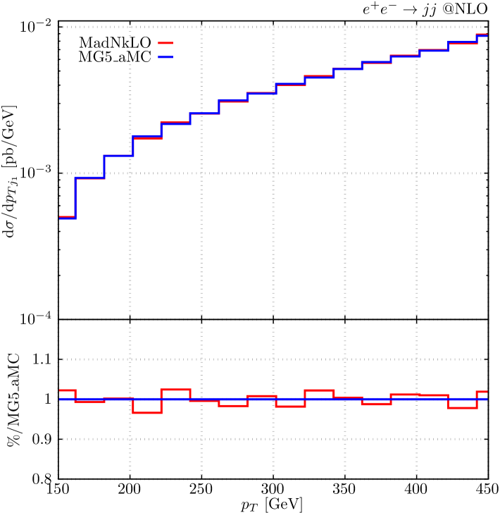
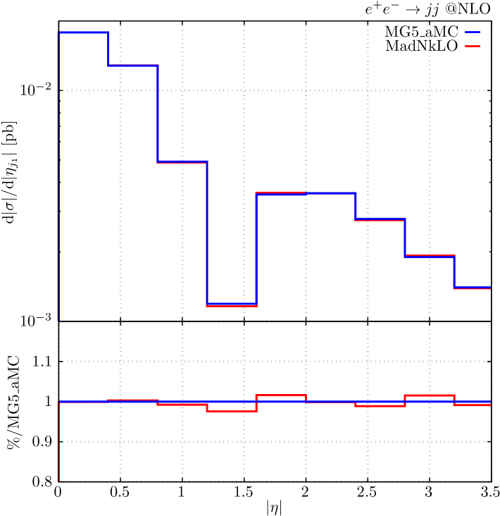
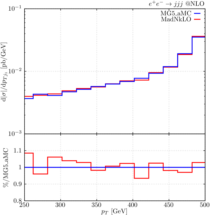
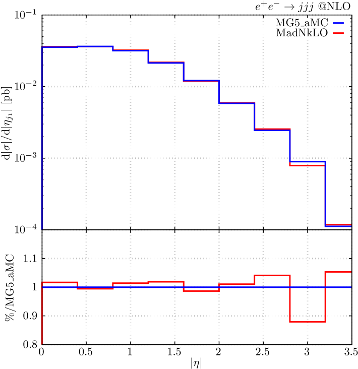
Figure 1: NLO correction to the transverse momentum (left column) and pseudo-rapidity (right column) of the leading jet for two-jet (upper row) and three-jet (bottom row) production in $e^{+}e^{-}$ annihilation. Blue and red curves are obtained with MadGraph5_aMC@NLO and MadNkLO, respectively. The insets display bin-by-bin ratios to the MadGraph5_aMC@NLO baseline.

the transverse momentum ($p_{Tj_{1}}$) and pseudo-rapidity ($\eta_{j_{1}}$) of the leading jet. Since we are considering NLO corrections alone, distributions are not necessarily positive-definite, in which case we plot the absolute value of the differential cross sections. Full agreement is observed between MadNkLO and MadGraph5_aMC@NLO over the whole ranges displayed. Statistical fluctuations are comparable for two-jet production, while slightly more pronounced for MadNkLO in the three-jet case. This may be related to the coexistence of different soft phase-space mappings within each partition, which will be the subject of a future dedicated analysis, beyond the scope of this article.

We then turn to the validation of massive QCD processes at NLO. We consider the leptonic production of $t\bar{t}$, $b\bar{b}$, and $t\bar{b}$ final states, which allows to probe the massive subtraction of Section 2 in different energy regimes.

In Fig. 2 we collect same-flavour production processes, $t\bar{t}$, $b\bar{b}$, and display the transverse momentum and pseudo-rapidity of the heavy quark (as opposed to anti-quark). We find consistent agreement with respect to MadGraph5_aMC@NLO.

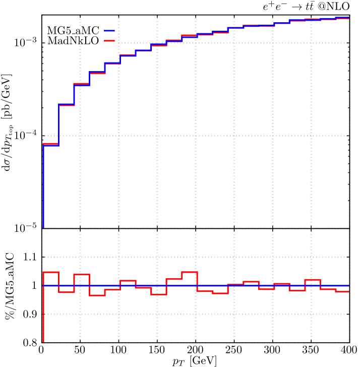
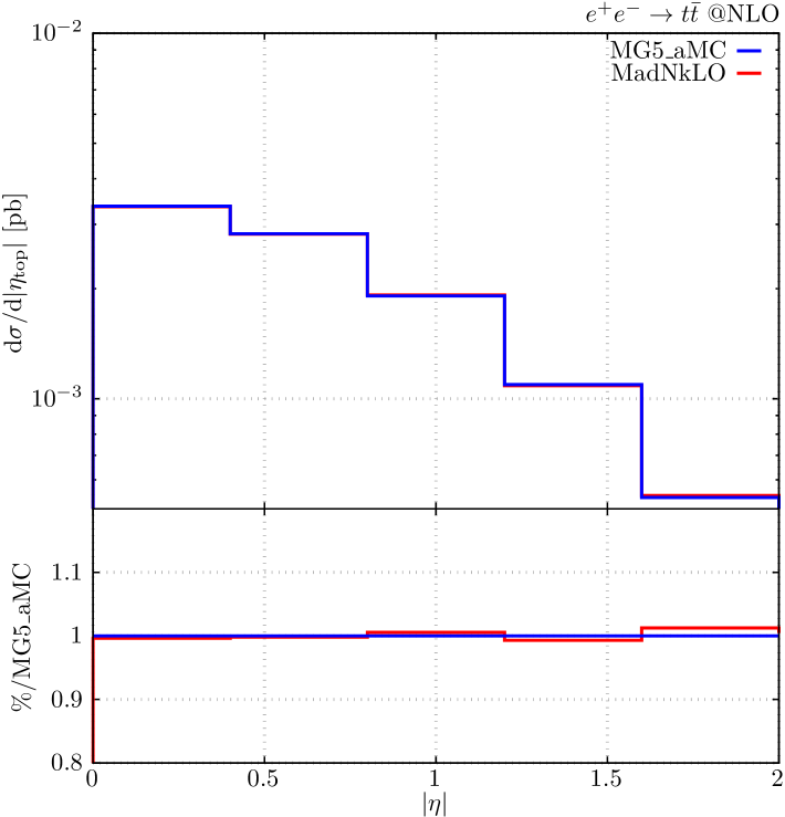
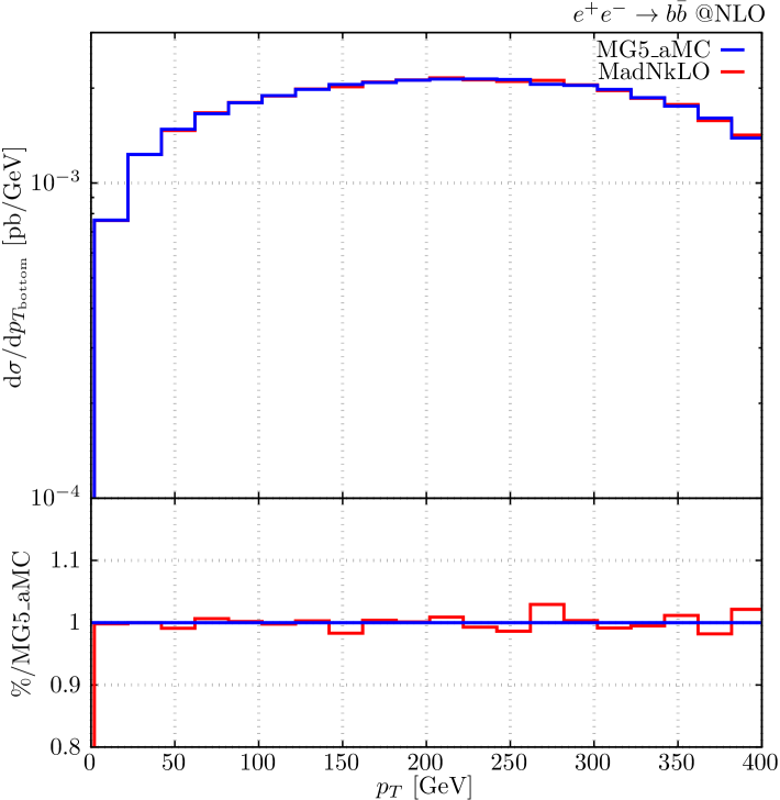
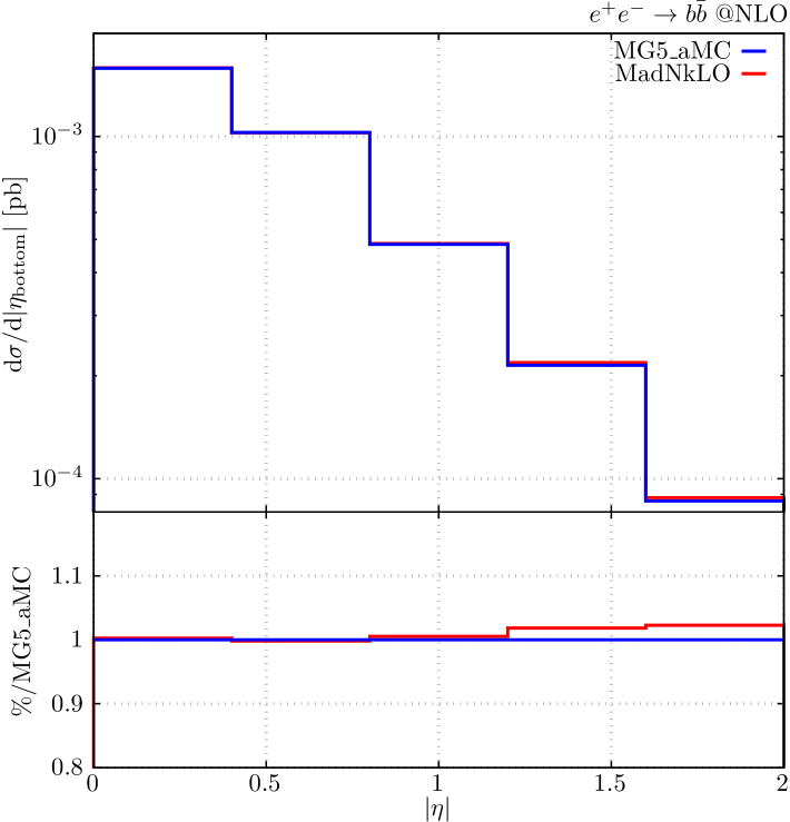
Figure 2: Same as in Fig. 1 for $t\bar{t}$ (upper row) and $b\bar{b}$ (bottom row) leptonic production.

An even more stringent test of the massive subtraction is provided by $t\bar{b}$ production. The large mass hierarchy between top and bottom quarks validates the subtraction in presence of a multi-scale problem, as well as in asymmetric-mass conditions. In Fig. 3 we display the transverse momentum and pseudo-rapidity of the top quark, again witnessing full agreement between MadNkLO and MadGraph5_aMC@NLO. For the considered massive processes, we observe a remarkable numerical stability of the MadNkLO results: the MadNkLO curves displayed in Figs. 2 and 3

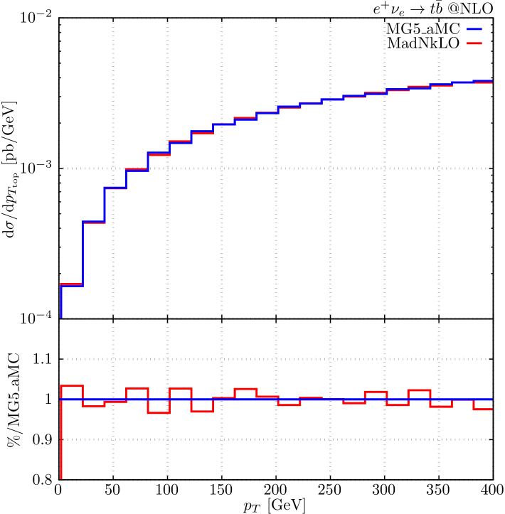
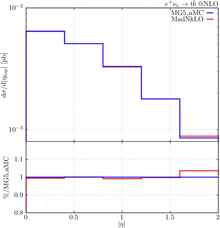
Figure 3: Same as in Fig. 1 for the charged-current process $e^{+}\nu_{e}\to t\bar{b}$.

were obtained using only a fraction of the phase-space points employed in MadGraph5_aMC@NLO, resulting in systematically shorter run times.

Given the evidence collected in this section, we consider our MadNkLO validation fully satisfactory, and move on to NNLO developments.

3.2 Numerical validation at NNLO

In Bertolotti:2022aih an analytic formula was obtained, within Local Analytic Sector Subtraction, for the cancellation of NNLO IR singularities in the case of massless final-state QCD radiation. In this section we take the first steps towards a thorough numerical implementation of that formula, and present numerical tests of singularity cancellation in a case study. The relevant definitions are collected in Appendix D.

We consider the process of di-jet production in $e^{+}e^{-}$ annihilation, and focus on the $e^{+}e^{-}\rightarrow q\bar{q}q^{\prime}\bar{q}^{\prime}$ radiative channel contributing to the NNLO double-real differential cross section. Moreover, we select the 3-particle symmetrised sector $\mathcal{Z}_{\{q\bar{q}q^{\prime}\}}$, defined in Eq. (157), in which the subtracted double-real correction schematically reads

$$RR^{\,\rm sub}_{\{q\bar{q}q^{\prime}\}}\,=\,RR\;\mathcal{Z}_{\{q\bar{q}q^{\prime}\}}-K^{\,(\mathbf{1})}_{\{q\bar{q}q^{\prime}\}}-K^{\,(\mathbf{2})}_{\{q\bar{q}q^{\prime}\}}+K^{\,(\mathbf{12})}_{\{q\bar{q}q^{\prime}\}}\,.$$ (36)

Here, $RR$ stands for the squared double-real matrix element, while $K^{\,(\mathbf{1})}_{\{q\bar{q}q^{\prime}\}}$, $K^{\,(\mathbf{2})}_{\{q\bar{q}q^{\prime}\}}$, and $K^{\,(\mathbf{12})}_{\{q\bar{q}q^{\prime}\}}$ collect the single-unresolved, the uniform double-unresolved, and the strongly-ordered double-unresolved subtraction counterterms, respectively.

For the selected sector, and given the particle content, phase-space singularities stem from the single-unresolved collinear limit, ${\bf C}_{q\bar{q}}$, from the double-unresolved double-soft limit ${\bf S}_{q\bar{q}}$, and from the uniform triple-collinear limit ${\bf C}_{q\bar{q}q^{\prime}}$. Correspondingly, the underlying real-emission and Born processes are $e^{+}e^{-}\rightarrow gq^{\prime}\bar{q}^{\prime}$, and $e^{+}e^{-}\rightarrow q^{\prime}\bar{q}^{\prime}$, respectively. The flavour of the particles involved in the sector also determines the physical content of the counterterms, which read

$$K^{\,(\mathbf{1})}_{\{q\bar{q}q^{\prime}\}} = \overline{\bf C}_{q\bar{q}}\,RR\;\mathcal{Z}_{\{q\bar{q}q^{\prime}\}}\,,$$

$$K^{\,(\mathbf{2})}_{\{q\bar{q}q^{\prime}\}} = \left(\,\overline{\bf S}_{q\bar{q}}+\overline{\bf HC}_{q\bar{q}q^{\prime}}\right)RR\;\mathcal{Z}_{\{q\bar{q}q^{\prime}\}}\,,$$

$$K^{\,(\mathbf{12})}_{\{q\bar{q}q^{\prime}\}} = \overline{\bf C}_{q\bar{q}}\,\left(\,\overline{\bf S}_{q\bar{q}}+\overline{\bf HC}_{q\bar{q}q^{\prime}}\right)RR\;\mathcal{Z}_{\{q\bar{q}q^{\prime}\}}\,,$$ (37)

where the hard-triple-collinear counterterm is defined as

$$\overline{\bf HC}_{q\bar{q}q^{\prime}}\,\equiv\,\overline{\bf C}_{q\bar{q}q^{\prime}}\left(1-\overline{\bf S}_{q\bar{q}}\right)\,,$$ (38)

and explicit expressions for all of these subtraction terms are provided in Eq. (D).

The tests to be performed to confirm a succesful singularity cancellation can be grouped into two sets:

$$\big{\{}{\bf C}_{ij},\;{\bf S}_{ij},\;{\bf C}_{ijk}\big{\}}\,RR^{\,\rm sub}_{\{ijk\}} \to \mbox{integrable}\,,$$ (39)

$$\big{\{}{\bf C}_{kr},\;{\bf C}_{ijr},\;{\bf C}_{ikr},\;{\bf C}_{jkr}\big{\}}\,RR^{\,\rm sub}_{\{ijk\}} \to \mbox{integrable}\,,$$ (40)

where $(ijk)=(q\bar{q}q^{\prime})$, and $r=\bar{q}^{\prime}$ sets the recoiler assignment for this sector. Eq. (39) collects the singular configurations of $RR\;\mathcal{Z}_{\{q\bar{q}q^{\prime}\}}$, that are supposed to be tamed by the presence of counterterms in $RR^{\,\rm sub}_{\{ijk\}}$, by construction. A detailed account of the expected cancellation pattern is reported in Eqs. (• ‣ D)–(• ‣ D). Eq. (40) contains collinear limits involving the recoiler particle $r$. The necessity for checking such configurations originates from the presence of the recoiler in the definition of the collinear splitting kernels: this could in principle give rise to a spurious singular behaviour of the counterterms when the recoiler is collinear to one or more of the partons defining the sector.

The cancellation test proceeds as follows. We obtain an $(n+2)$-body phase-space point by building two consecutive radiations on top of a generated Born configuration. Adopting Catani-Seymour parametrisations, the integration measure corresponding to the double-real radiation is written in terms of six kinematic variables, $w^{\prime},y^{\prime},z^{\prime}$, and $\phi/\pi,y,z$, each with support in $[0,1]$. Unprimed variables parametrise the first radiation, passing from $n$ to $(n+1)$ final-state particles, while primed quantities describe the radiation of the $(n+2)$-th parton. We report in Eq. (163) the specific double-radiative phase space that was used for the numerical test reported in the following.

As the azimuthal variables, $w^{\prime}$ and $\phi$, are not connected to IR singularities, the cancellation test focuses on the other four Catani-Seymour variables, without loss of generality. Given their expressions in terms of kinematic invariants, reported in Eq. (D), different IR-singular configurations are reached by scaling appropriate combinations of such variables to 0 or 1. As an example, the single-collinear limit ${\bf C}_{ij}$ is obtained by scaling $y^{\prime}$ to 0, leaving the other variables unchanged; conversely, a double-soft configuration ${\bf S}_{ij}$ implies $y^{\prime}$, $z$, and $y$ to approach 0 at the same rate. The scalings required to probe all singular configurations of Eqs. (39), (40) are collected in Table 2.

Limit	${\bf C}_{ij}$	${\bf S}_{ij}$	${\bf C}_{ijk}$	${\bf C}_{kr}$	${\bf C}_{ijr}$	${\bf C}_{ikr}$	${\bf C}_{jkr}$
$z^{\prime}$	–	–	–	–	–	0	1
$y^{\prime}$	0	0	0	–	–	–	–
$z$	–	0	–	1	0	1	1
$y$	–	0	0	–	–	–	–

Table 2: IR scaling behaviour of the kinematic variables $(z^{\prime},y^{\prime},z,y)$ as defined by the Catani-Seymour mapping of Eq. (D). Numerical entries (0 or 1) indicate the limiting value of the variables in the given IR configuration, while the ‘–’ symbol means that the corresponding variable is not scaled.

We assign a common scaling parameter $\lambda$ to all phase-space variables relevant to a given IR limit, so that the limit is reached in all cases when $\lambda\to 0$. For instance, considering Table 2, in the collinear ${\bf C}_{ij}$ limit one sets $y^{\prime}\sim\lambda$, while to probe the spurious ${\bf C}_{ikr}$ configuration, one sets $z^{\prime}\sim\lambda$, and $z\sim 1-\lambda$.

The results of running the cancellation checks of Eq. (39) on the subtracted double-real contribution $RR^{\,\rm sub}_{\{q\bar{q}q^{\prime}\}}$ are displayed in Fig. 4. The figure collects six panels, organised in two columns and three rows. Each row is dedicated to a different singular configuration in Eq. (39), corresponding to the following physical assignments to variable $\lambda$:

$${\bf C}_{ij}\,:\,\lambda\sim\theta_{ij}^{2}\rightarrow 0\,,\qquad{\bf S}_{ij}\,:\,\lambda\sim E_{i},\,E_{j}\rightarrow 0\,,\qquad{\bf C}_{ijk}\,:\,\lambda\sim\theta_{ij}^{2},\,\theta_{ik}^{2}\rightarrow 0\,.$$ (41)

For each of these IR limits, the left panels in Fig. 4 represent the absolute scaling of each contribution to $RR^{\,\rm sub}_{\{q\bar{q}q^{\prime}\}}$ as the limit is approached ($\lambda\to 0$). All terms are multiplied by the common phase-space jacobian (second line of Eq. (163)), and plotted as a function of $\lambda$. The right panels in Fig. 4 collect the various counterterms, as well as their sum, again as functions of $\lambda$, normalised to the unsubtracted double-real matrix element $RR$.

From the plots on the left column one immediately evinces that the subtracted double-real matrix element (blue dotted) has a visibly milder scaling with respect to the unsubtracted one (teal solid), as $\lambda$ approaches 0. In particular, in the ${\bf C}_{ij}$, ${\bf S}_{ij}$, ${\bf C}_{ijk}$ limits, respectively, the $RR$ behaviour $(\lambda^{-1},\lambda^{-3},\lambda^{-2})$ is reduced to $(\lambda^{-1/2},\lambda^{-2},\lambda^{-3/2})$ after subtraction. This confirms the successful cancellation of leading-power singularities by means of the counterterms defined in Eq. (3.2). The leftover behaviour of $RR^{\,\rm sub}_{\{q\bar{q}q^{\prime}\}}$ as a function of $\lambda$ can be assessed considering the scaling of the phase-space measure, which in the three singular limits is $d\lambda\times(\lambda^{0},\lambda^{2},\lambda^{1})$, respectively. Combining these informations, one can conclude that the subtracted double-real cross section is finite in the double-soft limit, while it features square-root integrable singularities in the collinear limits.

The cancellation of the leading IR singularities is similarly appreciated in the right plots of Fig. 4, where all counterterm contributions (dotted), together with their sum (blue solid – labelled as ‘Sum of CTs’), are displayed as ratios to the double-real matrix element (teal solid). As $\lambda$ decreases, each individual quantity stabilises towards a constant value. Notably, the overall sum (blue solid) correctly converges to unity, indicating that the coefficient of the leading-power singularity in $RR$ is precisely reproduced by the combined subtraction counterterms.

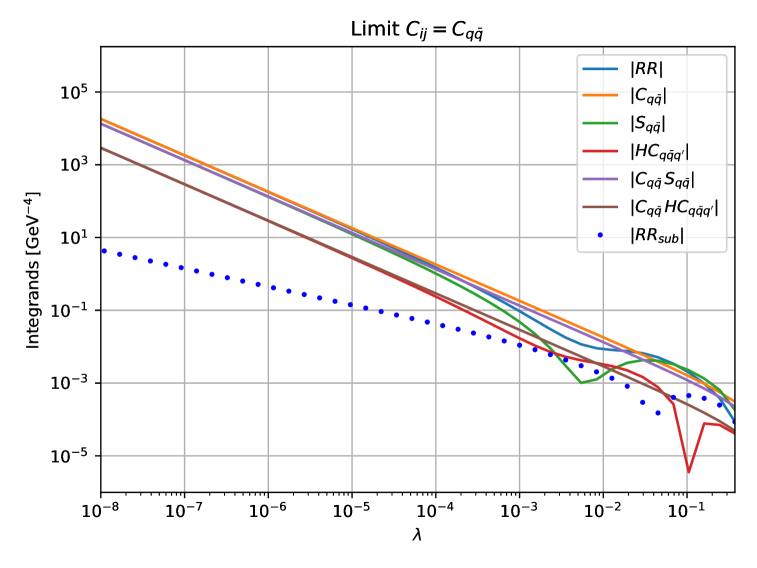
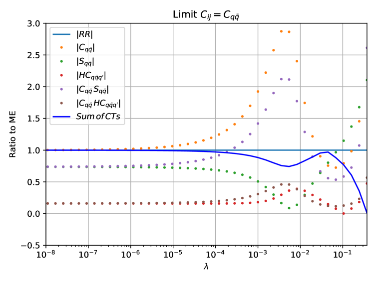
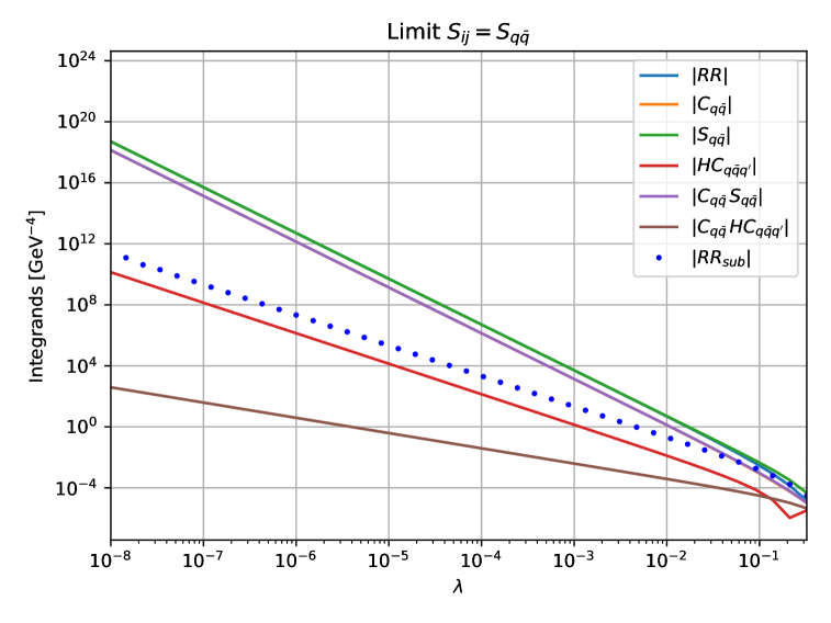
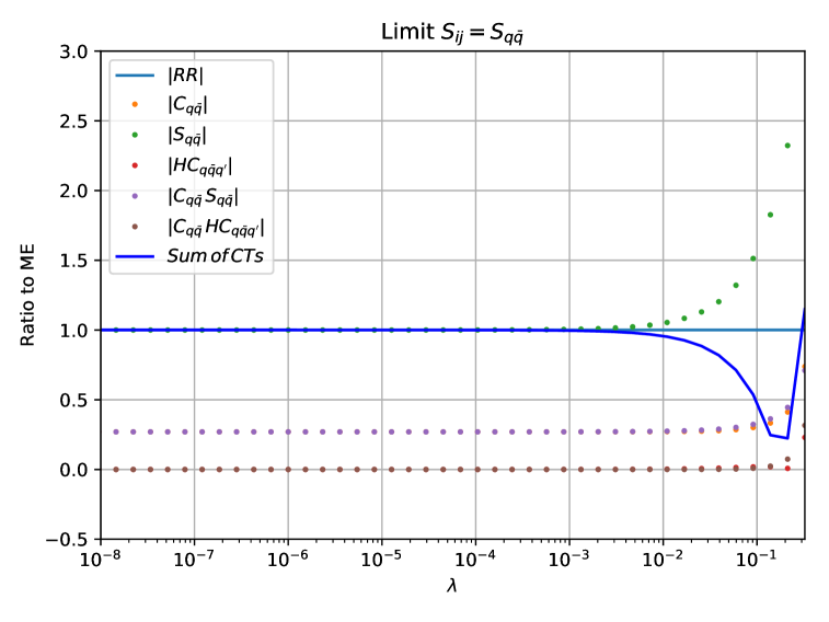
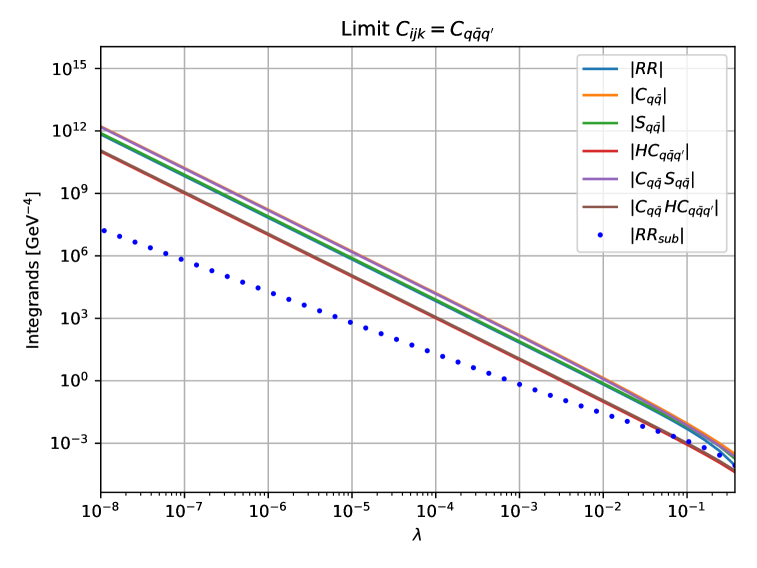
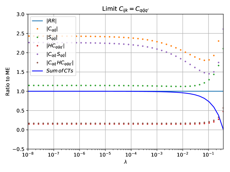
Figure 4: Scaling behaviour of the double-real matrix element and of the subtraction counterterms for the process $e^{+}e^{-}\rightarrow q\bar{q}q^{\prime}\bar{q}^{\prime}$, in sector $\mathcal{Z}_{\{q\bar{q}q^{\prime}\}}$. Top row: single-collinear limit ${\bf C}_{ij}$. Middle row: double-soft limit ${\bf S}_{ij}$. Bottom row: triple-collinear limit ${\bf C}_{ijk}$. Further details are in the main text.

The same reasoning just described can be applied to the study of the spurious collinear limits listed in Eq. (40). The plots presented in the top row of Fig. 5 reveal a regular behaviour for each individual counterterm, as well as for the double-real matrix element, in the ${\bf C}_{kr}$ and ${\bf C}_{ijr}$ limits. As for the ${\bf C}_{ikr}$ and ${\bf C}_{jkr}$ limits, displayed in the bottom row of Fig. 5, both the unsubtracted and the subtracted double-real matrix elements have a singular $\lambda^{-1/3}$ behaviour. This is integrable in nature, whence we conclude that all spurious limits are as well under control.

Figure 5: Scaling behaviour of the double-real matrix element and of the subtraction counterterms for the process $e^{+}e^{-}\rightarrow q\bar{q}q^{\prime}\bar{q}^{\prime}$, in sector $\mathcal{Z}_{\{q\bar{q}q^{\prime}\}}$. Top row: single-collinear limit ${\bf C}_{kr}$, and triple-collinear limit ${\bf C}_{ijr}$. Bottom row: triple-collinear limits ${\bf C}_{ikr}$ and ${\bf C}_{jkr}$. Further details are in the main text.

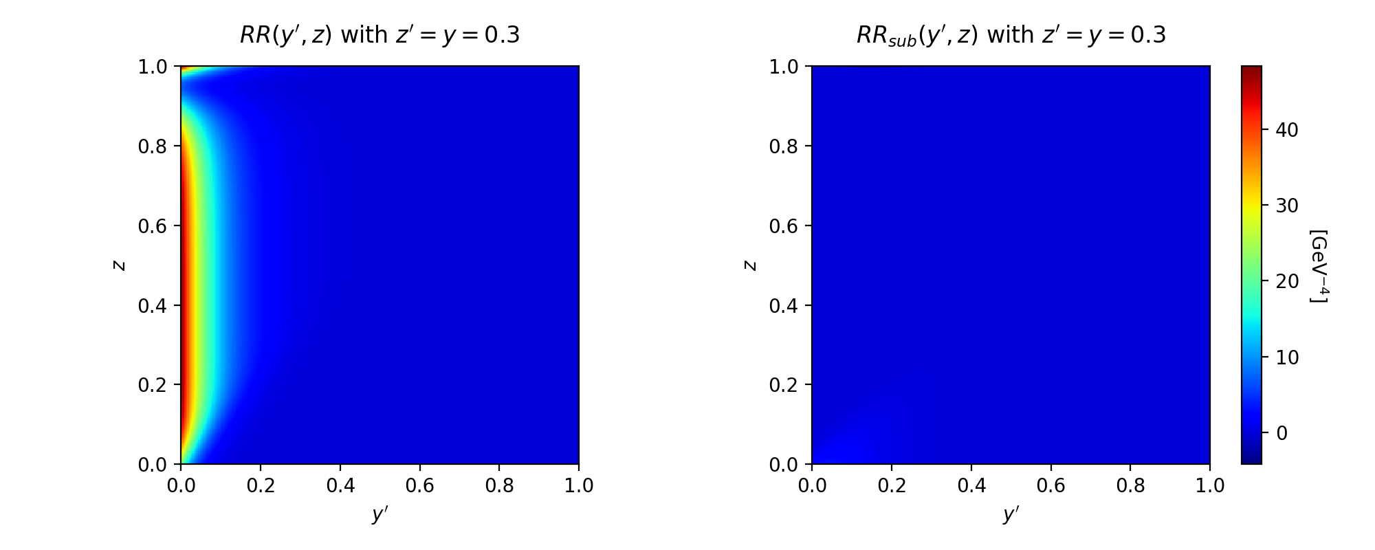
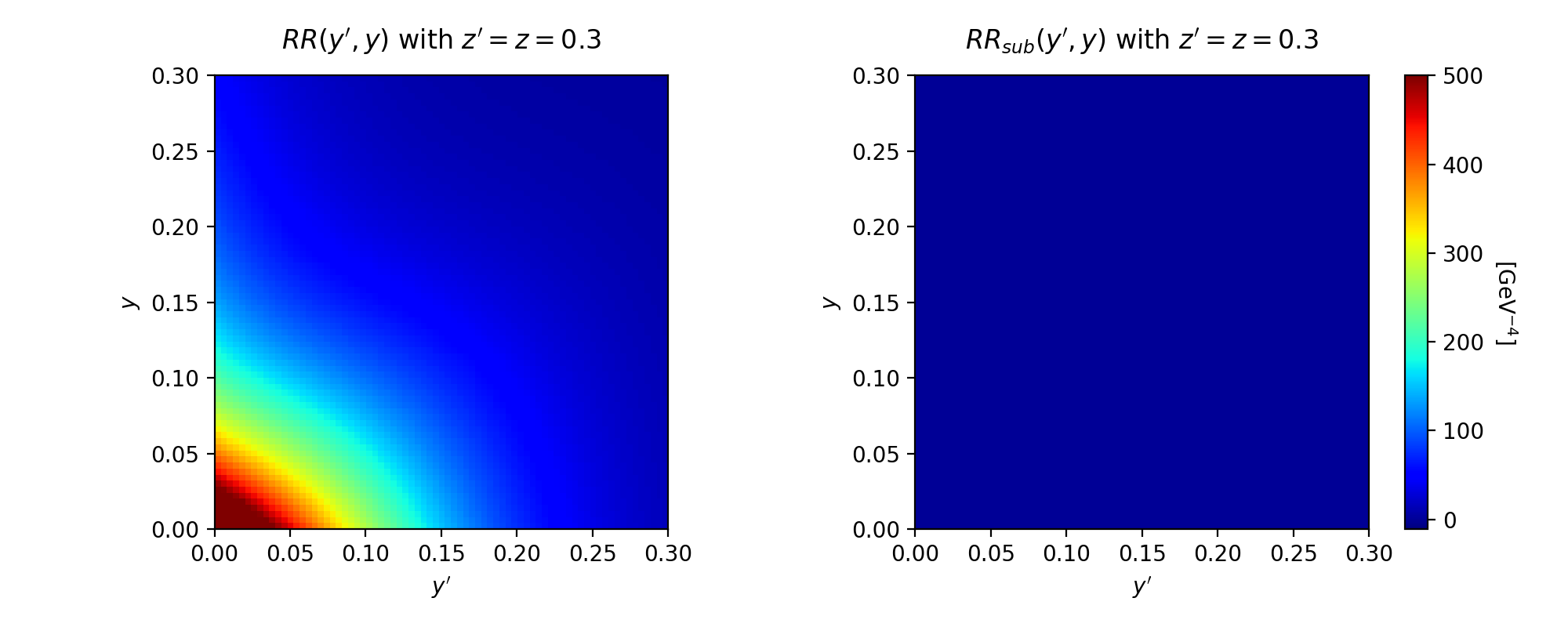
Figure 6: Density plots of the unsubtracted (left column) and subtracted (right column) double-real matrix element for two representative phase-space regions, in the process $e^{+}e^{-}\rightarrow q\bar{q}q^{\prime}\bar{q}^{\prime}$, within sector $\mathcal{Z}_{\{q\bar{q}q^{\prime}\}}$. Further details are in the main text.

As a further supporting evidence for singularity cancellation, we probed the double-real correction in representative portions of the phase space where IR divergences are expected to arise. The density plots in Fig. 6 present the result of such an analysis, where we sample the unsubtracted (left columns) and the subtracted (right columns) double-real matrix elements, respectively. In the top row, we fix $z^{\prime}=y=0.3$, and vary the remaining $y^{\prime},z$ variables over their entire $[0,1]\times[0,1]$ support. The upper left plot clearly shows an enhancement in $RR$ extending over the entire $z$ range, at $y^{\prime}\to 0$. As indicated in Table 2, this corresponds to the presence of the single-collinear singularity ${\bf C}_{ij}$ in the unsubtracted double-real correction. In contrast, the corresponding density plot for the subtracted contribution $RR^{\,\rm sub}$ (top right) is regular in the whole region, confirming a successful cancellation.

The phase-space configuration shown in the bottom row of Fig. 6 is obtained by setting $z^{\prime}=z=0.3$, while varying $y^{\prime}$ and $y$. In the lower left plot, a strong divergent peak appears in the $y^{\prime}\sim y\rightarrow 0$ limit, which corresponds to the triple-collinear singularity ${\bf C}_{ijk}$, as detailed in Table 2. The latter is effectively mitigated by the subtraction counterterms, as demonstrated by the stable behaviour of $RR^{\,\rm sub}$ in the lower right plot.

These considerations conclude the analysis of IR singularities, demonstrating the finiteness of the subtracted double-real matrix element for the considered channel in sector $\mathcal{Z}_{\{q\bar{q}q^{\prime}\}}$.

4 Conclusion

In this article we have presented a number of developments in the framework of Local Analytic Sector Subtraction. First, we have considered the NLO IR subtraction in presence of massive QCD particles in the final state. We have defined and analytically integrated all massive IR counterterms, reproducing the known singularity structure of one-loop massive matrix elements. As a designing feature, Local Analytic Sector Subtraction uses different phase-space mappings and parametrisations for different contributions to a given IR counterterm. This ensures the phase space to be optimally aligned with the natural Lorentz invariants appearing in each contribution, and in turn entails a comparatively simpler analytic counterterm integration. In the massive NLO case considered here, this structural simplicity is particularly evident in the finite parts of the integrated counterterms, which feature at worst di-logarithms for some of the soft contributions, and up to simple logarithms for hard-collinear terms. Such a simplicity has been attained via a thorough exploration of the phase-space symmetries, and their translation into new parametrisations of the integration measures. This analysis not only allowed us to simplify the integrations, as in the case of the soft NLO counterterm with two massive colour sources, but also gives the freedom of choosing phase-space mappings independently of the analytic integration. The latter feature constitutes a relevant starting point in view of the integration of NNLO double-soft massive kernels, which we leave for future work.

After the analytic discussion of NLO massive subtraction, we have turned our attention to the numerical implementation of the subtraction scheme, starting at NLO and documenting the validation of a variety of processes featuring QCD in the final state. The implementation is carried out in the MadNkLO framework, which offers the level of generality required for an automated generation of NLO differential cross sections. We have described the steps we have taken to overcome the original technical limitations of MadNkLO, in terms of phase-space generation, integration of the matrix elements, execution speed, and stability of the results. These features and the newly introduced massive NLO subtraction have been validated through a successful comparison with benchmark MadGraph5_aMC@NLO results, for processes with either massless or massive QCD particles in the final state.

Since MadNkLO is designed to host subtraction schemes at NNLO (and beyond), we have reported the first elements of the automated implementation of Local Analytic Sector Subtraction at NNLO within the MadNkLO framework. The implementation has so far been limited to the counterterms relevant to $e^{+}e^{-}\to q\bar{q}q^{\prime}\bar{q}^{\prime}$, namely a contribution to the quark channel in the production of two hadronic jets via leptonic collisions at NNLO in QCD. We have shown the complete cancellation of the single- and double-unresolved singularities of the double-real matrix elements, providing first non-trivial evidence of the stability performances of our NNLO implementation. The natural future development in this direction is the complete MadNkLO implementation of NNLO Local Analytic Sector Subtraction for final-state QCD radiation, of which this article represents a first important step.

Appendix A Mappings and radiative phase space with massive particles

In this appendix we detail the phase-space mappings relevant for the case of massive particles in the final state. Moreover, we explore different parametrisations of the radiative phase space, exploiting its symmetries to simplify analytic counterterm integration.

A.1 Final-final mapping with two massive final-state particles

Given three different final-state momenta $k_{a}$, $k_{b}$, $k_{c}$ with squared masses

$$k_{a}^{2}=0\,,\qquad k_{b}^{2}=m_{b}^{2}\,,\qquad k_{c}^{2}=m_{c}^{2}\,,$$ (42)

we construct the mapped momenta

$$\{\bar{k}\}^{(abc)}\,\equiv\,\Big{\{}\{k\}_{\not{a}\not{b}\not{c}},\bar{k}_{b}^{(abc)},\bar{k}_{c}^{(abc)}\Big{\}}\,.$$ (43)

Momenta $\bar{k}_{b}\equiv\bar{k}_{b}^{(abc)}$ and $\bar{k}_{c}\equiv\bar{k}_{c}^{(abc)}$ are given by

$$\theta_{{b}\in{\rm M}}\,\theta_{{c}\in{\rm M}}:\quad\bar{k}_{c}^{\mu} = \sqrt{\frac{\bar{s}^{2}-4m_{b}^{2}m_{c}^{2}}{s_{[ab]c}^{2}-4m_{c}^{2}(s_{ab}+m_{b}^{2})}}\left(k_{c}^{\mu}-\frac{s_{[ab]c}+2m_{c}^{2}}{2Q^{2}}Q^{\mu}\right)+\frac{\bar{s}+2m_{c}^{2}}{2Q^{2}}\,Q^{\mu}\,,$$

$$\bar{k}_{b}^{\mu} = Q^{\mu}-\bar{k}_{c}^{\mu}\,,$$ (44)

where $s_{ij}=2\,k_{i}\cdot k_{j}$ and

$$\bar{s}\,=\,s_{abc}\,=\,s_{ab}+s_{bc}+s_{ac}\,=\,Q^{2}-m_{b}^{2}-m_{c}^{2}\,,\qquad\quad s_{[ab]c}\,=\,s_{ac}+s_{bc}\,.$$ (45)

All other momenta are left unchanged by the mapping, namely $\bar{k}_{i}^{\mu}=k_{i}^{\mu}$ with $i\neq a,b,c$. Such definitions guarantee that the Born-level momenta $\bar{k}_{b}$ and $\bar{k}_{c}$ satisfy mass-shell conditions and total momentum conservation, as

$$\bar{k}_{b}^{2}\,=\,k_{b}^{2}\,=\,m_{b}^{2}\,,\qquad\bar{k}_{c}^{2}\,=\,k_{c}^{2}\,=\,m_{c}^{2}\,,\qquad Q^{\mu}\,=\,k_{a}^{\mu}+k_{b}^{\mu}+k_{c}^{\mu}\,=\,\bar{k}_{b}^{\mu}+\bar{k}_{c}^{\mu}\,.$$ (46)

The mapping $\{\bar{k}\}^{(abc)}$ induces an exact phase-space factorisation

$$\int d\Phi_{n+1}\,=\,\frac{\varsigma_{n+1}}{\varsigma_{n}}\int d\Phi_{n}^{(abc)}\int d\Phi_{\rm rad,\scriptscriptstyle{{\rm M}}\scriptscriptstyle{{\rm M}}}^{(abc)}\,,$$ (47)

where $d\Phi_{n}^{(abc)}\equiv d\Phi_{n}(\{\bar{k}\}^{(abc)})$ and we explicitly extracted the ratio of the relevant symmetry factors $\varsigma_{n+1}$ and $\varsigma_{n}$. The radiative phase-space measure associated with the unresolved particle $k_{a}$ can be parametrised in terms of the usual Catani-Seymour kinematic variables Catani:1996vz ; Catani:2002hc

$$z\,=\,\frac{s_{ac}}{s_{ac}+s_{bc}}\,,\qquad\qquad y\,=\,\frac{s_{ab}}{s_{ab}+s_{bc}+s_{ac}}\,,$$ (48)

yielding

$$s_{ab}\,=\,y\,\bar{s}\,,\qquad s_{ac}\,=\,z(1-y)\,\bar{s}\,,\qquad s_{bc}\,=\,(1-z)(1-y)\,\bar{s}\,.$$ (49)

According to Catani:2002hc , the parametrised radiative integration measure is

$$\int d\Phi_{\rm rad,\scriptscriptstyle{{\rm M}}\scriptscriptstyle{{\rm M}}}^{(abc)} = \frac{(2\pi)^{-3+2\epsilon}}{4}\,\bar{s}^{2-2\epsilon}\,\left(\sqrt{\lambda}\right)^{-1+2\epsilon}\int d^{d-3}\Omega$$ (50)

$$\hskip-11.38109pt\times\,\int_{0}^{y_{+}}dy\,(1-y)^{1-2\epsilon}(\bar{s}y+m_{b}^{2})^{-\epsilon}\int_{z_{-}(y)}^{z_{+}(y)}dz\,(z_{+}-z)^{-\epsilon}(z-z_{-})^{-\epsilon}\,,\qquad$$

where the integration boundaries are given by

$$y_{+}\,=\,1+\frac{2m_{c}^{2}}{\bar{s}}-\frac{2m_{c}Q}{\bar{s}}\,,\qquad z_{\pm}(y)\,=\,\frac{\bar{s}y}{2(\bar{s}y+m_{b}^{2})}\,\left(1\pm\frac{\sigma}{\bar{s}(1-y)}\right)\,,$$ (51)

and

$$\lambda = \bar{s}^{2}-4m_{b}^{2}m_{c}^{2}\,,$$

$$\sigma \equiv \sigma(y)\,=\,\sqrt{\lambda+\bar{s}^{2}y^{2}-2y\bar{s}(\bar{s}+2m_{c}^{2})}\,=\,\sqrt{\bar{s}^{2}(1-y)^{2}-4m_{c}^{2}(\bar{s}y+m_{b}^{2})}\,.$$ (52)

The integration over the solid angle can be carried out independently, yielding the factor

$$\int d^{d-3}\Omega\,=\,\frac{2\pi^{1-\epsilon}}{\Gamma(1-\epsilon)}\,,$$ (53)

so that

$$\int d\Phi_{\rm rad,\scriptscriptstyle{{\rm M}}\scriptscriptstyle{{\rm M}}}^{(abc)} = \frac{(4\pi)^{-2+\epsilon}\,\bar{s}}{\Gamma(1-\epsilon)}\left(\frac{\bar{s}}{\sqrt{\lambda}}\right)^{\!\!1-2\epsilon}$$

$$\qquad\times\,\int_{0}^{y_{+}}dy\,(1-y)^{1-2\epsilon}(\bar{s}y+m_{b}^{2})^{-\epsilon}\int_{z_{-}}^{z_{+}}dz\,(z_{+}-z)^{-\epsilon}(z-z_{-})^{-\epsilon}\,.$$

It is easy to verify that

$$\sigma(0)=\sqrt{\lambda}\,,\qquad\sigma(y_{+})=0\,,\qquad z_{\pm}(0)=0\,,\qquad z_{\pm}(y_{+})=\frac{\bar{s}y_{+}}{2(\bar{s}y_{+}+m_{b}^{2})}\,,$$ (55)

so that the integration domain is the region between the two curves $z=z_{\pm}(y)$, which meet at the endpoints

$$P_{1} \equiv \big{(}y,z_{\pm}(y)\big{)}|_{y=0}=\big{(}0,z_{\pm}(0)\big{)}=(0,0)\,,$$

$$P_{2} \equiv \big{(}y,z_{\pm}(y)\big{)}|_{y=y_{+}}=\big{(}y_{+},z_{\pm}(y_{+})\big{)}=\bigg{(}y_{+},\frac{\bar{s}y_{+}}{2(\bar{s}y_{+}+m_{b}^{2})}\bigg{)}\,.$$ (56)

The two curves satisfy the following equation:

$$z\,=\,z_{\pm}(y)\,=\,\frac{\bar{s}y}{2(\bar{s}y+m_{b}^{2})}\,\bigg{(}1\pm\frac{\sigma(y)}{\bar{s}(1-y)}\bigg{)}$$ (57)

$$\quad\Longrightarrow\quad \bar{s}\,y(1-y)^{2}z(1-z)-m_{b}^{2}\,(1-y)^{2}z^{2}-m_{c}^{2}\,y^{2}\,=\,0\,.$$

We now check how these curves transform under the exchange of $k_{b}$ with $k_{c}$. We introduce variables $Y,Z$ to re-parametrise the invariants in Eq. (49) under the exchange $k_{b}\leftrightarrow k_{c}$, as

$$s_{ab} = (1-Y)Z\,\bar{s}\,,\qquad s_{ac}\;=\;Y\,\bar{s}\,,\qquad s_{bc}\;=\;(1-Y)(1-Z)\,\bar{s}\,.$$ (58)

The change of variable $y,z\to Y,Z$ is thus defined by the relations $Z(1-Y)=y$, and $Y=z(1-y)$, which give

$$Y =\;z(1-y)\,, Z =\;\frac{y}{1-z(1-y)}\,,$$

$$y =\;Z(1-Y)\,, z =\;\frac{Y}{1-Z(1-Y)}\,.$$ (59)

In therms of the new variables, Eq. (57), defining the boundaries of the integration domain, becomes

$$\bar{s}\,Y(1-Y)^{2}Z(1-Z)-m_{b}^{2}\,Y^{2}-m_{c}^{2}\,(1-Y)^{2}Z^{2}\,=\,0\,.$$ (60)

This means that the re-parametrisation $y,z\to Y,Z$ is equivalent to the exchange $m_{b}\leftrightarrow m_{c}$. It is easy to verify that this holds in general for the radiative phase-space $d\Phi_{\rm rad,\scriptscriptstyle{{\rm M}}\scriptscriptstyle{{\rm M}}}^{(abc)}$. Indeed the Jacobian of the transformation reads

$$J(Y,Z) = \left|\frac{\partial y}{\partial Y}\,\frac{\partial z}{\partial Z}-\frac{\partial y}{\partial Z}\,\frac{\partial z}{\partial Y}\right|=\frac{1-Y}{1-Z(1-Y)}\,,\qquad$$ (61)

so that

$$dy\,dz\,(1-y) = dY\,dZ\,J(Y,Z)[1-Z(1-Y)]\;=\;dY\,dZ\,(1-Y)\,.$$ (62)

Furthermore, we can easily verify that

$$(1-y)^{2}(\bar{s}y+m_{b}^{2})(z_{+}-z)(z-z_{-}) = \bar{s}y(1-y)^{2}z(1-z)-m_{b}^{2}(1-y)^{2}z^{2}-m_{c}^{2}y^{2}$$

$$= \bar{s}Y(1-Y)^{2}Z(1-Z)-m_{b}^{2}Y^{2}-m_{c}^{2}(1-Y)^{2}Z^{2}$$

$$= (1-Y)^{2}(\bar{s}Y+m_{c}^{2})(Z_{+}-Z)(Z-Z_{-})\,,$$

where we have set

$$Y_{+}\,=\,1+\frac{2m_{b}^{2}}{\bar{s}}-\frac{2m_{b}Q}{\bar{s}}\,,\qquad\quad Z_{\pm}\,=\,\frac{\bar{s}Y}{2(\bar{s}Y+m_{c}^{2})}\,\bigg{(}1\pm\frac{\Sigma(Y)}{\bar{s}(1-Y)}\bigg{)}\,,$$

$$\Sigma(Y)\,=\,\sqrt{\lambda+\bar{s}^{2}Y^{2}-2Y\bar{s}(\bar{s}+2m_{b}^{2})}\,=\,\sqrt{\bar{s}^{2}(1-Y)^{2}-4m_{b}^{2}(\bar{s}Y+m_{c}^{2})}\,.$$ (63)

The radiative phase-space in Eq. (A.1) can then be equivalently rewritten as

$$\int d\Phi_{\rm rad,\scriptscriptstyle{{\rm M}}\scriptscriptstyle{{\rm M}}}^{(abc)} = \frac{(4\pi)^{-2+\epsilon}\,\bar{s}}{\Gamma(1-\epsilon)}\left(\frac{\bar{s}}{\sqrt{\lambda}}\right)^{\!\!1-2\epsilon}$$

$$\qquad\times\,\int_{0}^{Y_{+}}dY\,(1-Y)^{1-2\epsilon}(\bar{s}Y+m_{c}^{2})^{-\epsilon}\int_{Z_{-}}^{Z_{+}}dz\,(Z_{+}-Z)^{-\epsilon}(Z-Z_{-})^{-\epsilon}\,.$$

A parametrisation that makes the $b\leftrightarrow c$ symmetry more evident is the one in terms of variables $u,v$ defined by $(1-v)(1-u)=y$ and $u=(1-z)(1-y)$, which gives

$$u =\;(1-z)(1-y)\,, v =\;\frac{z(1-y)}{y+z-yz}\,,$$

$$y =\;(1-u)(1-v)\,, z =\;\frac{v(1-u)}{u+v-uv}\,.$$ (65)

The Jacobian of the transformation reads

$$J(u,v) = \left|\frac{\partial y}{\partial u}\,\frac{\partial z}{\partial v}-\frac{\partial y}{\partial v}\,\frac{\partial z}{\partial u}\right|\,=\,\frac{1-u}{u+v-uv}\,,$$ (66)

yielding

$$dy\,dz\,(1-y) = du\,dv\,J(u,v)\,(u+v-uv)\;=\;du\,dv\,(1-u)\,.$$ (67)

In addition, we have

$$(1-y)^{2}(\bar{s}y+m_{b}^{2})(z_{+}-z)(z-z_{-}) = \bar{s}\,y(1-y)^{2}z(1-z)-m_{b}^{2}\,(1-y)^{2}z^{2}-m_{c}^{2}\,y^{2}$$ (68)

$$= (1-u)^{2}\Big{[}\bar{s}\,u\,v(1-v)-m_{b}^{2}\,v^{2}-m_{c}^{2}\,(1-v)^{2}\Big{]}$$

$$= (1-u)^{2}(\bar{s}u+m_{b}^{2}+m_{c}^{2})(v_{+}-v)(v-v_{-})\,,\qquad\qquad$$

where $v_{\pm}$ are the solutions of the equation $\bar{s}uv(1-v)-m_{b}^{2}v^{2}-m_{c}^{2}(1-v)^{2}=0$, and read

$$v_{\pm}=v_{\pm}(u) = \frac{\bar{s}u+2m_{c}^{2}\pm\sqrt{\bar{s}^{2}u^{2}-4m_{b}^{2}m_{c}^{2}}}{2(\bar{s}u+m_{b}^{2}+m_{c}^{2})}\,.$$ (69)

In terms of $u$ and $v$, Eq. (57) becomes

$$(1-u)^{2}\Big{[}\bar{s}\,u\,v(1-v)-m_{b}^{2}\,v^{2}-m_{c}^{2}\,(1-v)^{2}\Big{]}\,=\,0\,,$$ (70)

or equivalently

$$(1-u)^{2}(\bar{s}u+m_{b}^{2}+m_{c}^{2})(v_{+}(u)-v)(v-v_{-}(u))=0\,.$$ (71)

That is to say that the two curves defining the integration domain of $v$ are $v=v_{\pm}(u)$. One has that $v_{+}(u)\geq v_{-}(u)$ for all values of $u\in[u_{-},1]$, the two curves being equal only for

$$u=u_{-}=\frac{2\,m_{b}\,m_{c}}{\bar{s}}\,.$$ (72)

We thus conclude that the integration domain in the $u,v$ parametrisation reads

$$\int_{0}^{y_{+}}dy\,\int_{z_{-}(y)}^{z_{+}(y)}dz\,(1-y) = \int_{u_{-}}^{1}du\,\int_{v_{-}(u)}^{v_{+}(u)}dv\,(1-u)\,.$$ (73)

The radiative phase space can thus be rewritten as

$$\int\!d\Phi_{\rm rad,\scriptscriptstyle{{\rm M}}\scriptscriptstyle{{\rm M}}}^{(abc)} = \frac{(4\pi)^{-2+\epsilon}\,\bar{s}}{\Gamma(1-\epsilon)}\left(\frac{\bar{s}}{\sqrt{\lambda}}\right)^{\!\!1-2\epsilon}$$

$$\qquad\times\,\int_{u_{-}}^{1}du\,(1-u)^{1-2\epsilon}(\bar{s}u+m_{b}^{2}+m_{c}^{2})^{-\epsilon}\int_{v_{-}}^{v_{+}}dv(v_{+}\!-\!v)^{-\epsilon}(v-v_{-})^{-\epsilon}\,,$$

with

$$s_{ab}=(1-u)(1-v)\,\bar{s}\,,\qquad s_{ac}=(1-u)v\,\bar{s}\,,\qquad s_{bc}=u\,\bar{s}\,.$$ (75)

A.2 Final-final mapping with one massive particle

The cases involving three final-state momenta, only one of which being massive, are special cases of the fully massive mapping considered in Appendix A.1. We report them explicitly in the following, for completeness.

Case $m_{b}=0$
In the $m_{b}=0$ case, we have

$$\theta_{{b}\in{\rm F}}\,\theta_{{c}\in{\rm M}}:\quad\bar{k}_{c}^{\mu} = \frac{\bar{s}}{\sqrt{s_{[ab]c}^{2}-4m_{c}^{2}s_{ab}}}\left(k_{c}^{\mu}-\frac{s_{[ab]c}+2m_{c}^{2}}{2(\bar{s}+m_{c}^{2})}Q^{\mu}\right)+\frac{\bar{s}+2m_{c}^{2}}{2(\bar{s}+m_{c}^{2})}Q^{\mu}\,,$$

$$\bar{k}_{b}^{\mu} = Q^{\mu}-\bar{k}_{c}^{\mu}\,.$$ (76)

The relevant quantities defining the radiative integration measure in the three provided parametrisations are

$$y_{+}\,=\,1+\frac{2m_{c}^{2}}{\bar{s}}-\frac{2m_{c}\sqrt{\bar{s}+m_{c}^{2}}}{\bar{s}}\,,\qquad Y_{+}\,=\,1\,,$$

$$\lambda=\bar{s}^{2}\,,\qquad\sigma(y)\,=\,\sqrt{\bar{s}^{2}(1-y)^{2}-4m_{c}^{2}\,\bar{s}\,y}\,,\qquad\Sigma(Y)\;=\;\bar{s}\,(1-Y)\,,$$

$$z_{\pm}\,=\,\frac{1}{2}\,\bigg{(}1\pm\frac{\sigma}{\bar{s}(1-y)}\bigg{)}\,,\qquad Z_{-}\,=\,0\,,\qquad Z_{+}\,=\,\frac{\bar{s}Y}{\bar{s}Y+m_{c}^{2}}\,,$$

$$u_{-}=0\,,\qquad v_{-}=\frac{m_{c}^{2}}{\bar{s}u+m_{c}^{2}}\,,\qquad v_{+}=1\,.$$ (77)

The phase-space measure then reads

$$\int d\Phi_{\rm rad,\scriptscriptstyle{{\rm F}}\scriptscriptstyle{{\rm M}}}^{(abc)} = \frac{(4\pi)^{-2+\epsilon}}{\Gamma(1-\epsilon)}\,\bar{s}^{1-\epsilon}\,\int_{0}^{y_{+}}dy\,y^{-\epsilon}\,(1-y)^{1-2\epsilon}\int_{z_{-}}^{z_{+}}dz\,(z_{+}-z)^{-\epsilon}(z-z_{-})^{-\epsilon}$$

$$= \frac{(4\pi)^{-2+\epsilon}\,\bar{s}}{\Gamma(1-\epsilon)}\,\int_{0}^{1}dY\,(1-Y)^{1-2\epsilon}(\bar{s}Y+m_{c}^{2})^{-\epsilon}\int_{0}^{Z_{+}}dZ\,Z^{-\epsilon}(Z_{+}-Z)^{-\epsilon}$$

$$= \frac{(4\pi)^{-2+\epsilon}\,\bar{s}}{\Gamma(1-\epsilon)}\int_{0}^{1}du\,(1-u)^{1-2\epsilon}(\bar{s}u+m_{c}^{2})^{-\epsilon}\int_{v_{-}}^{1}dv\,(1-v)^{-\epsilon}(v-v_{-})^{-\epsilon}\,.$$

We notice that in this case $z_{\pm}=1-z_{\mp}$: the phase-space measure is symmetric under the exchange $a\leftrightarrow b$, which corresponds to the variable transformation $z\leftrightarrow 1-z$.

Case $m_{c}=0$
Similarly, in the $m_{c}=0$ case, we have

$$\theta_{{b}\in{\rm M}}\,\theta_{{c}\in{\rm F}}:\quad\bar{k}_{c}^{\mu} = \frac{\bar{s}}{s_{[ab]c}}\,k_{c}^{\mu}\;=\;\frac{s_{abc}}{s_{[ab]c}}\,k_{c}^{\mu}\,,$$

$$\bar{k}_{b}^{\mu} = k_{a}^{\mu}+k_{b}^{\mu}-\frac{s_{ab}}{s_{[ab]c}}\,k_{c}^{\mu}\,,$$ (79)

which are identical to the fully massless case. The relevant quantities defining the integration measure in the three provided parametrisations are

$$y_{+}\,=\,1\,,\qquad Y_{+}\,=\,1+\frac{2m_{b}^{2}}{\bar{s}}-\frac{2m_{b}\sqrt{\bar{s}+m_{b}^{2}}}{\bar{s}}\,,\qquad$$

$$\lambda=\bar{s}^{2}\,,\qquad\sigma(y)\,=\,\bar{s}\,(1-y)\,,\qquad\Sigma(Y)\;=\;\sqrt{\bar{s}^{2}(1-Y)^{2}-4m_{b}^{2}\,\bar{s}\,Y}\,,\qquad$$

$$z_{-}\,=\,0\,,\qquad z_{+}\,=\,\frac{\bar{s}y}{\bar{s}y+m_{b}^{2}}\,,\qquad Z_{\pm}\,=\,\frac{1}{2}\,\bigg{(}1\pm\frac{\Sigma(Y)}{\bar{s}(1-Y)}\bigg{)}\,,\qquad$$

$$u_{-}=0\,,\qquad v_{-}=0\,,\qquad v_{+}=\frac{\bar{s}u}{\bar{s}u+m_{b}^{2}}\,.$$ (80)

The phase-space measure becomes

$$\int d\Phi_{\rm rad,\scriptscriptstyle{{\rm M}}\scriptscriptstyle{{\rm F}}}^{(abc)} = \frac{(4\pi)^{-2+\epsilon}\,\bar{s}}{\Gamma(1-\epsilon)}\,\int_{0}^{1}dy\,(1-y)^{1-2\epsilon}(\bar{s}y+m_{b}^{2})^{-\epsilon}\int_{0}^{z_{+}}dz\,z^{-\epsilon}(z_{+}-z)^{-\epsilon}$$ (81)

$$= \frac{(4\pi)^{-2+\epsilon}}{\Gamma(1-\epsilon)}\,\bar{s}^{1-\epsilon}\,\int_{0}^{Y_{+}}dY\,Y^{-\epsilon}\,(1-Y)^{1-2\epsilon}\int_{Z_{-}}^{Z_{+}}dZ\,(Z_{+}-Z)^{-\epsilon}(Z-Z_{-})^{-\epsilon}$$

$$= \frac{(4\pi)^{-2+\epsilon}\,\bar{s}}{\Gamma(1-\epsilon)}\int_{0}^{1}du\,(1-u)^{1-2\epsilon}(\bar{s}u+m_{b}^{2})^{-\epsilon}\int_{0}^{v_{+}}dv\,v^{-\epsilon}(v_{+}-v)^{-\epsilon}\,.$$

We stress that the relation $d\Phi_{\rm rad,\scriptscriptstyle{{\rm F}}\scriptscriptstyle{{\rm M}}}(Y,Z,m_{c})=d\Phi_{\rm rad,\scriptscriptstyle{{\rm M}}\scriptscriptstyle{{\rm F}}}(y,z,m_{b})$, valid in the massive-massless case, directly stems from the equivalence between Eq. (A.1) and Eq. (A.1). This in turn is what allows to get the same expression for the two integrated massive-massless soft kernels in Eq. (23).

A.3 Initial-final mapping with one massive particle

Given two final-state momenta $k_{a}$, $k_{b}$ and one initial-state momentum $k_{c}$, with masses

$$k_{a}^{2}=0\,,\qquad k_{b}^{2}=m_{b}^{2}\,,\qquad k_{c}^{2}=0\,,$$ (82)

we construct the mapped momenta

$$\{\bar{k}\}^{(abc)}\,=\,\Big{\{}\{k\}_{\not{a}\not{b}\not{c}},\bar{k}_{b}^{(abc)},\bar{k}_{c}^{(abc)}\Big{\}}\,,$$ (83)

where $\bar{k}_{b}\equiv\bar{k}_{b}^{(abc)}$ and $\bar{k}_{c}\equiv\bar{k}_{c}^{(abc)}$ are given by

$$\theta_{{b}\in{\rm M}}\theta_{{c}\in{\rm I}}:\quad\bar{k}^{(abc)}_{b} = k_{a}+k_{b}-\frac{s_{ab}}{s_{ac}+s_{bc}}\,k_{c}\,,$$

$$\bar{k}^{(abc)}_{c} = \frac{s_{ac}+s_{bc}-s_{ab}}{s_{ac}+s_{bc}}\,k_{c}\,,$$ (84)

while all other momenta are left unchanged, $\bar{k}_{i}^{\mu}=k_{i}^{\mu}$ with $i\neq a,b,c$. Such transformations guarantee that the Born-level momenta $\bar{k}_{b}$ and $\bar{k}_{c}$ satisfy mass-shell conditions and total momentum conservation, as

$$\bar{k}_{b}^{2}\,=\,k_{b}^{2}\,=\,m_{b}^{2}\,,\qquad\bar{k}_{c}^{2}\,=\,k_{c}^{2}\,=\,0\,,\qquad Q^{\mu}\,=\,k_{a}^{\mu}+k_{b}^{\mu}-k_{c}^{\mu}\,=\,\bar{k}_{b}^{\mu}-\bar{k}_{c}^{\mu}\,.$$ (85)

The mapping $\{\bar{k}\}^{(abc)}$ induces the phase-space factorisation

$$\int d\Phi_{n+1}(k_{c})\,=\,\frac{\varsigma_{n+1}}{\varsigma_{n}}\int\int d\Phi_{n}^{(abc)}(xk_{c})\,d\Phi_{\rm rad}^{(abc)}\,,$$ (86)

where $d\Phi_{n}^{(abc)}(xk_{c})\equiv d\Phi_{n}(\{\bar{k}\}^{(abc)})$, and we explicitly extracted the ratio of the relevant symmetry factors $\varsigma_{n+1}$ and $\varsigma_{n}$. The radiative phase-space measure associated with the unresolved particle $k_{a}$ can be parametrised in terms of the following kinematic variables:

$$x\,=\,\frac{s_{ac}+s_{bc}-s_{ab}}{s_{ac}+s_{bc}}\,,\qquad\qquad z\,=\,\frac{s_{ac}}{s_{ac}+s_{bc}}\,.$$ (87)

The invariants constructed with momenta $k_{a}$, $k_{b}$, and $k_{c}$ can be written in terms of these integration variables, as

$$s_{ab}\,=\,(1-x)\,\bar{s}\,,\qquad\quad s_{ac}\,=\,z\,\bar{s}\,,\qquad\quad s_{bc}\,=\,(1-z)\,\bar{s}\,,$$ (88)

where

$$\bar{s}\,=\,\bar{s}_{bc}^{(abc)}\,=\,2\bar{k}_{b}^{(abc)}\cdot k_{c}\,=\,\frac{2\bar{k}_{b}^{(abc)}\cdot\bar{k}_{c}^{(abc)}}{x}\,=\,\frac{m_{b}^{2}-Q^{2}}{x}\,=\,\frac{s_{ac}+s_{bc}-s_{ab}}{x}\,.$$ (89)

The parametrised radiative integration measure Catani:2002hc reads

$$\int d\Phi_{\rm rad,\scriptscriptstyle{{\rm M}}\scriptscriptstyle{{\rm I}}}^{(abc)} = \frac{(2\pi)^{-3+2\epsilon}\,\bar{s}}{4}\,\int d^{d-3}\Omega\,\int_{0}^{1}\!dx\,\big{[}\bar{s}(1-x)+m_{b}^{2}\big{]}^{-\epsilon}\int_{0}^{z_{+}}\!dz\,(z_{+}-z)^{-\epsilon}z^{-\epsilon}\,,\qquad$$ (90)

with

$$z_{+}\,=\,\frac{\bar{s}(1-x)}{\bar{s}(1-x)+m_{b}^{2}}\,.$$ (91)

Upon integration over the solid angle, see Eq. (53), one gets

$$\int d\Phi_{\rm rad,\scriptscriptstyle{{\rm M}}\scriptscriptstyle{{\rm I}}}^{(abc)} = \frac{(4\pi)^{-2+\epsilon}\,\bar{s}}{\Gamma(1-\epsilon)}\,\int_{0}^{1}\!dx\,\big{[}\bar{s}(1-x)+m_{b}^{2}\big{]}^{-\epsilon}\int_{0}^{z_{+}}\!dz\,(z_{+}-z)^{-\epsilon}z^{-\epsilon}\,.\qquad$$ (92)

Appendix B Collinear kernels

We report here the Altarelli-Parisi kernels relevant for the final-state splitting of a parent parton $[ij]$ into a pair of collinear siblings $ij$:

$$P_{ij,\scriptscriptstyle{{\rm F}}}^{\mu\nu}(z_{i}) = -P_{ij,\scriptscriptstyle{{\rm F}}}(z_{i})\,g^{\mu\nu}+Q_{ij,\scriptscriptstyle{{\rm F}}}(z_{i})\,\bigg{[}\!-g^{\mu\nu}+(d-2)\,\frac{\widetilde{k}_{\scriptscriptstyle{{\rm F}}}^{\mu}\,\widetilde{k}_{\scriptscriptstyle{{\rm F}}}^{\nu}}{\widetilde{k}_{\scriptscriptstyle{{\rm F}}}^{2}}\bigg{]}\,,$$ (93)

with

$$P_{ij,\scriptscriptstyle{{\rm F}}}(z_{i}) = T_{R}\bigg{(}1-\frac{2z_{i}z_{j}}{1-\epsilon}\bigg{)}f_{ij}^{q\bar{q}}+C_{F}\bigg{[}\frac{2z_{i}}{z_{j}}+(1-\epsilon)z_{j}\bigg{]}\,f_{i}^{q,\bar{q}}\,f_{j}^{g}$$

$$+\,C_{F}\bigg{[}\frac{2z_{j}}{z_{i}}+(1-\epsilon)z_{i}\bigg{]}\,f_{i}^{g}\,f_{j}^{q,\bar{q}}+C_{A}\bigg{(}\frac{z_{i}}{z_{j}}+\frac{z_{j}}{z_{i}}+z_{i}z_{j}\bigg{)}f_{ij}^{gg}\,,$$

$$Q_{ij,\scriptscriptstyle{{\rm F}}}(z_{i}) = T_{R}\,\frac{2z_{i}z_{j}}{1-\epsilon}\,f_{ij}^{q\bar{q}}-2\,C_{A}\,z_{i}z_{j}\,f_{ij}^{gg}\,.$$ (94)

The longitudinal momentum fractions of partons $i$, $j$, and their transverse momenta with respect to the collinear direction are

$$z_{i}\,=\,\frac{s_{ir}}{s_{ir}+s_{jr}}\,=\,1-z_{j}\,,\qquad\widetilde{k}_{\scriptscriptstyle{{\rm F}}}^{\mu}\,=\,z_{j}\,k_{i}^{\mu}-z_{i}\,k_{j}^{\mu}-(z_{j}-z_{i})\frac{s_{ij}}{s_{ir}+s_{jr}}k_{r}^{\mu}\,.$$ (95)

Upon subtracting all soft enhancements from the kernels, one obtains the final-state hard-collinear splitting functions:

$$P_{ij,\scriptscriptstyle{{\rm F}}}^{\mu\nu,{\rm\,hc}}(z_{i}) = -P_{ij,\scriptscriptstyle{{\rm F}}}^{{\rm\,hc}}(z_{i})\,g^{\mu\nu}+Q_{ij,\scriptscriptstyle{{\rm F}}}(z_{i})\,\bigg{[}\!-g^{\mu\nu}+(d-2)\,\frac{\widetilde{k}_{\scriptscriptstyle{{\rm F}}}^{\mu}\,\widetilde{k}_{\scriptscriptstyle{{\rm F}}}^{\nu}}{\widetilde{k}_{\scriptscriptstyle{{\rm F}}}^{2}}\bigg{]}\,,$$ (96)

with

$$P_{ij,\scriptscriptstyle{{\rm F}}}^{\rm\,hc}(z_{i}) = P_{ij,\scriptscriptstyle{{\rm F}}}^{{\rm hc},({\rm 0g})}(z_{i})\,f_{ij}^{q\bar{q}}+P_{ij,\scriptscriptstyle{{\rm F}}}^{{\rm hc},({\rm 1g})}(z_{i})\,f_{i}^{q,\bar{q}}\,f_{j}^{g}$$

$$\hskip 68.2866pt+\,P_{ij,\scriptscriptstyle{{\rm F}}}^{{\rm hc},({\rm 1g})}(z_{j})\,f_{i}^{g}\,f_{j}^{q,\bar{q}}+P_{ij,\scriptscriptstyle{{\rm F}}}^{{\rm hc},({\rm 2g})}(z_{i})\,f_{ij}^{gg}\,,$$

$$P_{ij,\scriptscriptstyle{{\rm F}}}^{{\rm hc},({\rm 0g})}(z) = T_{R}\bigg{[}1-\frac{2z(1-z)}{1-\epsilon}\bigg{]}\,,$$

$$P_{ij,\scriptscriptstyle{{\rm F}}}^{{\rm hc},({\rm 1g})}(z) = C_{F}(1-\epsilon)(1-z)\,,$$

$$P_{ij,\scriptscriptstyle{{\rm F}}}^{{\rm hc},({\rm 2g})}(z) = 2C_{A}\,z(1-z)\,.$$ (97)

The kernels for the initial-state splitting of a parent parton $c=j$ (or $c=i$) into a pair of collinear siblings $ab=[ij]i$ (or $ab=[ji]j$) are

$$P_{ab,\scriptscriptstyle{{\rm I}}}^{\mu\nu}(x_{a}) = -P_{ab,\scriptscriptstyle{{\rm I}}}(x_{a})\,g^{\mu\nu}+Q_{ab,\scriptscriptstyle{{\rm I}}}(x_{a})\,\bigg{[}-g^{\mu\nu}+(d\!-\!2)\,\frac{\widetilde{k}_{\scriptscriptstyle{{\rm I}}}^{\mu}\,\widetilde{k}_{\scriptscriptstyle{{\rm I}}}^{\nu}}{\widetilde{k}_{\scriptscriptstyle{{\rm I}}}^{2}}\bigg{]}\,,$$ (98)

with

$$P_{ab,\scriptscriptstyle{{\rm I}}}(x_{a}) = P_{ab,\scriptscriptstyle{{\rm F}}}(x_{a})\,,$$

$$Q_{ab,\scriptscriptstyle{{\rm I}}}(x_{a}) = -2\,\frac{x_{b}}{x_{a}}\,C_{F}\,f_{a}^{g}\,f_{b}^{q,\bar{q}}-2\,\frac{x_{b}}{x_{a}}\,C_{A}\,f_{ab}^{gg}\,.$$ (99)

In this case, longitudinal fractions and transverse momenta are defined as

$$x_{b}\,=\,\frac{s_{br}}{s_{cr}}\,=\,1-x_{a}\,,\qquad\widetilde{k}_{\scriptscriptstyle{{\rm I}}}^{\mu}\,=\,k_{b}^{\mu}-x_{b}\,k_{c}^{\mu}-\frac{s_{bc}}{s_{cr}}\,k_{r}^{\mu}\,.\qquad$$ (100)

The hard-collinear version of the kernels reads

$$P_{ab,\scriptscriptstyle{{\rm I}}}^{\mu\nu,{\rm\,hc}}(x_{a}) = -P_{ab,\scriptscriptstyle{{\rm I}}}^{\rm\,hc}(x_{a})\,g^{\mu\nu}+Q_{ab,\scriptscriptstyle{{\rm I}}}(x_{a})\,\bigg{[}-\!g^{\mu\nu}+(d\!-\!2)\,\frac{\widetilde{k}_{\scriptscriptstyle{{\rm I}}}^{\mu}\,\widetilde{k}_{\scriptscriptstyle{{\rm I}}}^{\nu}}{\widetilde{k}_{\scriptscriptstyle{{\rm I}}}^{2}}\bigg{]}\,,$$

where we have defined

$$P_{ab,\scriptscriptstyle{{\rm I}}}^{\rm\,hc}(x_{a}) = P_{ab,\scriptscriptstyle{{\rm I}}}^{{\rm hc},({\rm 0g})}(x_{a})\,f_{ab}^{q\bar{q}}+P_{ab,\scriptscriptstyle{{\rm I}}}^{{\rm hc},({\rm 1g},{\rm qg})}(x_{a})\,f_{a}^{q,\bar{q}}\,f_{b}^{g}$$

$$\hskip 68.2866pt+\,P_{ab,\scriptscriptstyle{{\rm I}}}^{{\rm hc},({\rm 1g},{\rm gq})}(x_{a})\,f_{a}^{g}\,f_{b}^{q,\bar{q}}+P_{ab,\scriptscriptstyle{{\rm I}}}^{{\rm hc},({\rm 2g})}(x_{a})\,f_{ab}^{gg}\,,$$

$$P_{ab,\scriptscriptstyle{{\rm I}}}^{{\rm\,hc},({\rm 0g})}(x) = T_{R}\bigg{[}1-\frac{2\ x(1-x)}{1-\epsilon}\bigg{]}\,,$$

$$P_{ab,\scriptscriptstyle{{\rm I}}}^{{\rm\,hc},({\rm 1g},{\rm qg})}(x) = C_{F}(1-\epsilon)\,(1-x)\,,$$

$$P_{ab,\scriptscriptstyle{{\rm I}}}^{{\rm\,hc},({\rm 1g},{\rm gq})}(x) = C_{F}\bigg{[}\frac{1+(1-x)^{2}}{x}-\epsilon\,x\bigg{]}\,,$$

$$P_{ab,\scriptscriptstyle{{\rm I}}}^{{\rm\,hc},({\rm 2g})}(x) = 2C_{A}\bigg{[}\frac{1-x}{x}+x(1-x)\bigg{]}\,.$$ (101)

Appendix C Integration of massive counterterms

In this appendix we outline the integration of all NLO counterterms in presence of massive particles in the final state.

C.1 Integration of the fully massive soft counterterm

We start by analytically integrating the soft counterterm

$$I_{\rm s,\scriptscriptstyle{{\rm M}}\scriptscriptstyle{{\rm M}}}^{ikl} = \mathcal{N}_{1}\int d\Phi_{\rm rad,\scriptscriptstyle{{\rm M}}\scriptscriptstyle{{\rm M}}}^{(ikl)}\,\mathcal{E}_{kl}^{(i)}\,,$$ (102)

over the radiative phase space $d\Phi_{\rm rad,\scriptscriptstyle{{\rm M}}\scriptscriptstyle{{\rm M}}}^{(ikl)}$. This is obtained with the massive mapping of Eq. (10), with the identifications $a\to i$, $b\to k$, $c\to l$, recalling that parton $i$ is a gluon, thus massless. In Appendix A.1 we have introduced different equivalent parametrisations for $\int d\Phi_{\rm rad,\scriptscriptstyle{{\rm M}}\scriptscriptstyle{{\rm M}}}^{(abc)}$. To integrate the eikonal kernel $\mathcal{E}_{kl}^{(i)}$, which is symmetric under $k\leftrightarrow l$ exchange, it is best to use the symmetric parametrisation of Eq. (A.1). With the invariants of Eq. (75), the eikonal kernel reads

$$\mathcal{E}_{kl}^{(i)} = \mathcal{I}_{kl}^{(i)}-\frac{1}{2}\,\mathcal{I}_{kk}^{(i)}-\frac{1}{2}\,\mathcal{I}_{ll}^{(i)}=f_{i}^{g}\bigg{(}\frac{s_{kl}}{s_{ik}s_{il}}-\frac{m_{k}^{2}}{s_{ik}^{2}}-\frac{m_{l}^{2}}{s_{il}^{2}}\bigg{)}$$ (103)

$$= f_{i}^{g}\,\frac{1}{\bar{s}(1-u)^{2}}\bigg{[}\frac{u}{v(1-v)}-\frac{m_{k}^{2}}{\bar{s}(1-v)^{2}}-\frac{m_{l}^{2}}{\bar{s}v^{2}}\bigg{]}\,,$$

with $\bar{s}=\bar{s}_{kl}^{(ikl)}$. It is interesting to notice that the numerator of the eikonal kernel reproduces the $\epsilon$-dependent part of the phase-space measure:

$$\mathcal{E}_{kl}^{(i)} = f_{i}^{g}\,\frac{\bar{s}\,u\,v(1-v)-m_{k}^{2}\,v^{2}-m_{l}^{2}\,(1-v)^{2}}{\bar{s}^{2}(1-u)^{2}v^{2}(1-v)^{2}}$$ (104)

$$= f_{i}^{g}\,\frac{(\bar{s}u+m_{k}^{2}+m_{l}^{2})(v_{+}-v)(v-v_{-})}{\bar{s}^{2}(1-u)^{2}v^{2}(1-v)^{2}}\,.$$

The fully massive soft integral $I_{\rm s,\scriptscriptstyle{{\rm M}}\scriptscriptstyle{{\rm M}}}^{ikl}$ is then given by

$$I_{\rm s,\scriptscriptstyle{{\rm M}}\scriptscriptstyle{{\rm M}}}^{ikl} = f_{i}^{g}\,\mathcal{N}_{1}\,\frac{(4\pi)^{-2+\epsilon}}{\Gamma(1-\epsilon)}\!\left(\!\frac{\bar{s}}{\sqrt{\lambda}}\!\right)^{\!\!1-2\epsilon}\!\!\int_{u_{-}}^{1}\!\!\!\!du\,(1-u)^{-1-2\epsilon}(\bar{s}u\!+\!m_{k}^{2}\!+\!m_{l}^{2})^{-\epsilon}\!$$ (105)

$$\qquad\times\,\int_{v_{-}}^{v_{+}}\!\!\!\!dv\,(v_{+}\!-\!v)^{-\epsilon}(v\!-\!v_{-})^{-\epsilon}\bigg{[}\frac{u}{v}+\frac{u}{1-v}-\frac{m_{k}^{2}}{\bar{s}(1-v)^{2}}-\frac{m_{l}^{2}}{\bar{s}v^{2}}\bigg{]}\,,\qquad$$

with

$$\lambda=\bar{s}^{2}-4m_{k}^{2}m_{l}^{2}\,,\qquad u_{-}=\frac{2m_{k}m_{l}}{\bar{s}}\,,\qquad v_{\pm}=\frac{\bar{s}u+2m_{l}^{2}\pm\sqrt{\bar{s}^{2}u^{2}-4m_{k}^{2}m_{l}^{2}}}{2(\bar{s}u+m_{k}^{2}+m_{l}^{2})}\,.\qquad$$ (106)

The only singular behaviour giving raise to a pole in $\epsilon$ is for $u\to 1$. We thus subtract and add back the integrand at $u=1$:

$$I_{\rm s,\scriptscriptstyle{{\rm M}}\scriptscriptstyle{{\rm M}}}^{ikl} = I_{\rm s,\scriptscriptstyle{{\rm M}}\scriptscriptstyle{{\rm M}}}^{ikl(0)}+I_{\rm s,\scriptscriptstyle{{\rm M}}\scriptscriptstyle{{\rm M}}}^{ikl(1)}+\mathcal{O}(\epsilon)\,,$$ (107)

$$I_{\rm s,\scriptscriptstyle{{\rm M}}\scriptscriptstyle{{\rm M}}}^{ikl(0)} = f_{i}^{g}\,\frac{\alpha_{s}}{2\pi}\left(\frac{\bar{s}}{\mu^{2}}\right)^{\!\!-\epsilon}\!\!\left(\!\frac{\bar{s}}{\sqrt{\lambda}}\!\right)^{\!\!1-2\epsilon}\!\!\bigg{(}\frac{Q^{2}}{\bar{s}}\bigg{)}^{\!\!-\epsilon}\!\int_{u_{-}}^{1}\!\!\!\!du\,(1-u)^{-1-2\epsilon}$$

$$\qquad\qquad\times\,\int_{V_{-}}^{V_{+}}\!\!\!\!dv\,(V_{+}\!-\!v)^{-\epsilon}(v\!-\!V_{-})^{-\epsilon}\bigg{[}\frac{1}{1-v}+\frac{1}{v}-\frac{m_{k}^{2}}{\bar{s}(1-v)^{2}}-\frac{m_{l}^{2}}{\bar{s}v^{2}}\bigg{]}\,,$$

$$I_{\rm s,\scriptscriptstyle{{\rm M}}\scriptscriptstyle{{\rm M}}}^{ikl(1)} = f_{i}^{g}\,\frac{\alpha_{s}}{2\pi}\left(\frac{\bar{s}}{\mu^{2}}\right)^{\!\!-\epsilon}\frac{\bar{s}}{\sqrt{\lambda}}\int_{u_{-}}^{1}\!\!\frac{du}{1-u}\,\bigg{\{}\,\int_{v_{-}(u)}^{v_{+}(u)}\!\!\!\!dv\,\bigg{[}\frac{u}{1-v}+\frac{u}{v}-\frac{m_{k}^{2}}{\bar{s}(1-v)^{2}}-\frac{m_{l}^{2}}{\bar{s}v^{2}}\bigg{]}$$ (108)

$$\hskip 133.72795pt-\int_{v_{-}(1)}^{v_{+}(1)}\!\!\!\!dv\,\bigg{[}\frac{1}{1-v}+\frac{1}{v}-\frac{m_{k}^{2}}{\bar{s}(1-v)^{2}}-\frac{m_{l}^{2}}{\bar{s}v^{2}}\bigg{]}\bigg{\}}\,,\qquad$$

where we have set

$$V_{\pm}\,\equiv\,v_{\pm}(1)\,=\,\frac{\bar{s}+2m_{l}^{2}\pm\sqrt{\lambda}}{2(\bar{s}+m_{k}^{2}+m_{l}^{2})}\,.$$ (109)

To compute $I_{\rm s,\scriptscriptstyle{{\rm M}}\scriptscriptstyle{{\rm M}}}^{ikl(0)}$, it is useful to introduce the change of variable

$$v^{\prime}\,=\,\frac{v-V_{-}}{V_{+}-V_{-}}\,,\qquad\quad v=V_{-}+(V_{+}-V_{-})v^{\prime}\,,$$ (110)

thus obtaining

$$I_{\rm s,\scriptscriptstyle{{\rm M}}\scriptscriptstyle{{\rm M}}}^{ikl(0)} = f_{i}^{g}\,\frac{\alpha_{s}}{2\pi}\left(\frac{\bar{s}}{\mu^{2}}\right)^{-\epsilon}\frac{\bar{s}}{\sqrt{\lambda}}\,\left(\frac{\bar{s}\,Q^{2}}{\lambda}\right)^{-\epsilon}\int_{u_{-}}^{1}du\,(1-u)^{-1-2\epsilon}(V_{+}-V_{-})^{1-2\epsilon}$$ (111)

$$\hskip-11.38109pt\times\,\int_{0}^{1}dv^{\prime}\,[v^{\prime}(1-v^{\prime})]^{-\epsilon}\bigg{\{}\frac{1}{1-V_{-}-(V_{+}-V_{-})v^{\prime}}+\frac{1}{V_{-}+(V_{+}-V_{-})v^{\prime}}$$

$$\hskip 82.51299pt-\,\frac{m_{k}^{2}}{\bar{s}[1-V_{-}-(V_{+}-V_{-})v^{\prime}]^{2}}-\frac{m_{l}^{2}}{\bar{s}[V_{-}+(V_{+}-V_{-})v^{\prime}]^{2}}\bigg{\}}\,.\qquad$$

The $u$-integration generates a single $\epsilon$ pole, as anticipated

$$\int_{u_{-}}^{1}du\,(1-u)^{-1-2\epsilon} = \frac{(1-u_{-})^{-2\epsilon}}{-2\epsilon}\,=\,-\frac{1}{2\epsilon}+\ln\frac{\bar{s}-2m_{k}m_{l}}{\bar{s}}+\cal O(\epsilon)\,,$$ (112)

while the $v$-integration can be performed using the standard results

$$\int_{0}^{1}dv^{\prime}\,[v^{\prime}(1-v^{\prime})]^{-\epsilon}\frac{1}{av^{\prime}+b}\,=\,\frac{1}{a}\,\ln\frac{a+b}{b}+\frac{\epsilon}{a}\,\bigg{[}-\mbox{Li}_{2}\bigg{(}-\frac{a}{b}\bigg{)}+\mbox{Li}_{2}\bigg{(}\frac{a}{a+b}\bigg{)}\bigg{]}+{\cal O}(\epsilon^{2})\,,$$

$$\int_{0}^{1}dv^{\prime}\,[v^{\prime}(1-v^{\prime})]^{-\epsilon}\frac{1}{(av^{\prime}+b)^{2}}\,=\,\frac{1}{b(a+b)}\,\bigg{[}1+\epsilon\,\frac{a+2b}{a}\,\ln\frac{a+b}{b}\bigg{]}+{\cal O}(\epsilon^{2})\,.$$ (113)

Considering that

$$V_{+}-V_{-}\,=\,\frac{\sqrt{\lambda}}{\bar{s}+m_{k}^{2}+m_{l}^{2}}\,,\qquad V_{+}+V_{-}\,=\,\frac{\bar{s}+2m_{l}^{2}}{\bar{s}+m_{k}^{2}+m_{l}^{2}}\,,$$

$$2-V_{+}-V_{-}\,=\,\frac{\bar{s}+2m_{k}^{2}}{\bar{s}+m_{k}^{2}+m_{l}^{2}}\,,\qquad V_{+}V_{-}\,=\,\frac{m_{l}^{2}}{\bar{s}+m_{k}^{2}+m_{l}^{2}}\,,$$

$$(1-V_{+})(1-V_{-})\,=\,\frac{m_{k}^{2}}{\bar{s}+m_{k}^{2}+m_{l}^{2}}\,,\qquad\frac{V_{-}(1-V_{+})}{V_{+}(1-V_{-})}\,=\,\frac{\bar{s}-\sqrt{\lambda}}{\bar{s}+\sqrt{\lambda}}\,,\qquad$$ (114)

and using the di-logarithmic identity

$$\mbox{Li}_{2}\bigg{(}-\frac{2\sqrt{\lambda}}{\bar{s}+2m^{2}-\sqrt{\lambda}}\bigg{)} = -\mbox{Li}_{2}\bigg{(}\frac{2\sqrt{\lambda}}{\bar{s}+2m^{2}+\sqrt{\lambda}}\bigg{)}-\frac{1}{2}\,\ln^{2}\frac{\bar{s}+2m^{2}+\sqrt{\lambda}}{\bar{s}+2m^{2}-\sqrt{\lambda}}\,,\qquad$$ (115)

we get

$$I_{\rm s,\scriptscriptstyle{{\rm M}}\scriptscriptstyle{{\rm M}}}^{ikl(0)} = -\,f_{i}^{g}\,\frac{\alpha_{s}}{2\pi}\left(\frac{\bar{s}}{\mu^{2}}\right)^{-\epsilon}\frac{\bar{s}}{2\sqrt{\lambda}}\,\Bigg{\{}-\bigg{[}\frac{1}{\epsilon}+\ln\frac{Q^{2}\,\bar{s}}{(\bar{s}-2m_{k}m_{l})^{2}}\bigg{]}\bigg{[}\ln\frac{\bar{s}-\sqrt{\lambda}}{\bar{s}+\sqrt{\lambda}}+\frac{2\sqrt{\lambda}}{\bar{s}}\bigg{]}$$ (116)

$$\hskip 42.67912pt+\,\frac{1}{2}\,\ln^{2}\frac{\bar{s}+2m_{k}^{2}+\sqrt{\lambda}}{\bar{s}+2m_{k}^{2}-\sqrt{\lambda}}-\frac{2m_{k}^{2}}{\bar{s}}\,\ln\frac{\bar{s}+2m_{k}^{2}+\sqrt{\lambda}}{\bar{s}+2m_{k}^{2}-\sqrt{\lambda}}$$

$$\hskip 42.67912pt+\frac{1}{2}\,\ln^{2}\frac{\bar{s}+2m_{l}^{2}+\sqrt{\lambda}}{\bar{s}+2m_{l}^{2}-\sqrt{\lambda}}-\frac{2m_{l}^{2}}{\bar{s}}\,\ln\frac{\bar{s}+2m_{l}^{2}+\sqrt{\lambda}}{\bar{s}+2m_{l}^{2}-\sqrt{\lambda}}+\ln\frac{\bar{s}-\sqrt{\lambda}}{\bar{s}+\sqrt{\lambda}}$$

$$\hskip 42.67912pt+\,2\,\mbox{Li}_{2}\bigg{(}\frac{2\sqrt{\lambda}}{\bar{s}+2m_{k}^{2}+\sqrt{\lambda}}\bigg{)}+2\,\mbox{Li}_{2}\bigg{(}\frac{2\sqrt{\lambda}}{\bar{s}+2m_{l}^{2}+\sqrt{\lambda}}\bigg{)}+{\cal O}(\epsilon)\Bigg{\}}\,.\qquad$$

Next, we introduce the convenient notation

$$\eta_{k,l}=\frac{\bar{s}+2m_{k,l}^{2}-\sqrt{\lambda}}{\bar{s}+2m_{k,l}^{2}+\sqrt{\lambda}}\,,\qquad\qquad\eta=\eta_{k}\,\eta_{l}=\frac{\bar{s}-\sqrt{\lambda}}{\bar{s}+\sqrt{\lambda}}\,,\qquad$$ (117)

and arrive at our final expression for $I_{\rm s,\scriptscriptstyle{{\rm M}}\scriptscriptstyle{{\rm M}}}^{ikl(0)}$:

$$I_{\rm s,\scriptscriptstyle{{\rm M}}\scriptscriptstyle{{\rm M}}}^{ikl(0)} = f_{i}^{g}\,\frac{\alpha_{s}}{2\pi}\left(\frac{\bar{s}}{\mu^{2}}\right)^{-\epsilon}\Bigg{\{}\bigg{[}\frac{1}{\epsilon}+\ln\frac{Q^{2}\,\bar{s}}{(\bar{s}-2m_{k}m_{l})^{2}}\bigg{]}\bigg{[}\frac{\bar{s}}{2\sqrt{\lambda}}\ln\eta+1\bigg{]}$$ (118)

$$\hskip 85.35826pt-\,\frac{\bar{s}}{\sqrt{\lambda}}\,\bigg{[}\mbox{Li}_{2}(1-\eta_{k})+\mbox{Li}_{2}(1-\eta_{l})+\frac{1}{8}\ln^{2}\frac{\eta_{k}}{\eta_{l}}+\frac{\ln^{2}\eta}{8}\bigg{]}$$

$$\hskip 85.35826pt-\,\frac{m_{k}^{2}-m_{l}^{2}}{2\sqrt{\lambda}}\ln\frac{\eta_{k}}{\eta_{l}}-\frac{Q^{2}}{2\sqrt{\lambda}}\ln\eta+{\cal O}(\epsilon)\Bigg{\}}\,.$$

We now turn to the computation of $I_{\rm s,\scriptscriptstyle{{\rm M}}\scriptscriptstyle{{\rm M}}}^{ikl(1)}$. We first perform the $v$-integration, making use of the following relations:

$$v_{+}v_{-}=\frac{m_{l}^{2}}{\bar{s}u+m_{k}^{2}+m_{l}^{2}}\,,\qquad(1-v_{+})(1-v_{-})=\frac{m_{k}^{2}}{\bar{s}u+m_{k}^{2}+m_{l}^{2}}\,,$$

$$v_{+}-v_{-}=\frac{\sqrt{\bar{s}^{2}u^{2}-4m_{k}^{2}m_{l}^{2}}}{\bar{s}u+m_{k}^{2}+m_{l}^{2}}\,,\qquad\frac{v_{-}(1-v_{+})}{v_{+}(1-v_{-})}=\frac{\bar{s}u-\sqrt{\bar{s}^{2}u^{2}-4m_{k}^{2}m_{l}^{2}}}{\bar{s}u+\sqrt{\bar{s}^{2}u^{2}-4m_{k}^{2}m_{l}^{2}}}\,,$$ (119)

and get

$$I_{\rm s,\scriptscriptstyle{{\rm M}}\scriptscriptstyle{{\rm M}}}^{ikl(1)} = f_{i}^{g}\,\frac{\alpha_{s}}{2\pi}\left(\frac{\bar{s}}{\mu^{2}}\right)^{-\epsilon}\frac{\bar{s}}{\sqrt{\lambda}}\int_{u_{-}}^{1}\frac{du}{1-u}\,\bigg{[}-\,u\,\ln\frac{\bar{s}u-\sqrt{\bar{s}^{2}u^{2}-4m_{k}^{2}m_{l}^{2}}}{\bar{s}u+\sqrt{\bar{s}^{2}u^{2}-4m_{k}^{2}m_{l}^{2}}}+\ln\eta$$ (120)

$$\hskip 133.72795pt-\,2\,\frac{\sqrt{\bar{s}^{2}u^{2}-4m_{k}^{2}m_{l}^{2}}}{\bar{s}}+2\,\frac{\sqrt{\lambda}}{\bar{s}}\bigg{]}\,.$$

At this point, we perform a change of variables to get rid of the square root. Denoting as $u_{1}$ and $u_{2}$ the two roots of the quadratic equation $\bar{s}^{2}u^{2}-4m_{k}^{2}m_{l}^{2}=0$, namely

$$u_{1}\,=\,\frac{2m_{k}m_{l}}{\bar{s}}\,=\,u_{-}\,,\qquad\qquad u_{2}\,=\,-\,\frac{2m_{k}m_{l}}{\bar{s}}\,,$$ (121)

we introduce the variables

$$t\,=\,\sqrt{\frac{u-u_{1}}{u-u_{2}}}\,,\qquad\qquad\beta = \sqrt{\frac{1-u_{1}}{1-u_{2}}}\,=\,\sqrt{\frac{\bar{s}-2m_{k}m_{l}}{\bar{s}+2m_{k}m_{l}}}\,.$$ (122)

This modifies the integration measure as follows:

$$u\,=\,\frac{2m_{k}m_{l}}{\bar{s}}\,\frac{1+t^{2}}{1-t^{2}}\,,\qquad 1-u\,=\,\frac{\bar{s}+2m_{k}m_{l}}{\bar{s}}\,\frac{\beta^{2}-t^{2}}{1-t^{2}}\,,$$

$$\sqrt{\bar{s}^{2}u^{2}-4m_{k}^{2}m_{l}^{2}}\,=\,4m_{k}m_{l}\,\frac{t}{1-t^{2}}\,,\qquad\int_{u_{-}}^{1}du\,=\,\frac{4m_{k}m_{l}}{\bar{s}}\int_{0}^{\beta}\frac{2t\,dt}{(1-t^{2})^{2}}\,.$$ (123)

The constants appearing in the $t$-integration can be recast in terms of the sole variable $\beta$, with the help of the following relations:

$$1-\beta^{2}\,=\,\frac{4m_{k}m_{l}}{\bar{s}+2m_{k}m_{l}}\,,\qquad\qquad\frac{\beta}{1-\beta^{2}}\,=\,\frac{\sqrt{\lambda}}{4m_{k}m_{l}}\,,$$

$$\frac{1+\beta^{2}}{1-\beta^{2}}\,=\,\frac{\bar{s}}{2m_{k}m_{l}}\,,\qquad\qquad\bigg{(}\frac{1-\beta}{1+\beta}\bigg{)}^{2}\,=\,\frac{\bar{s}-\sqrt{\lambda}}{\bar{s}+\sqrt{\lambda}}\,=\,\eta\,.$$ (124)

The $I_{\rm s,\scriptscriptstyle{{\rm M}}\scriptscriptstyle{{\rm M}}}^{ikl(1)}$ integral then becomes

$$I_{\rm s,\scriptscriptstyle{{\rm M}}\scriptscriptstyle{{\rm M}}}^{ikl(1)} = -\,f_{i}^{g}\,\frac{\alpha_{s}}{2\pi}\left(\frac{\bar{s}}{\mu^{2}}\right)^{-\epsilon}\frac{\bar{s}}{\sqrt{\lambda}}\,\frac{4m_{k}m_{l}}{\bar{s}}\,\int_{0}^{\beta}dt\,$$ (125)

$$\qquad\times\,\bigg{[}\frac{1+\beta^{2}}{1-\beta^{2}}\bigg{(}\frac{1}{\beta-t}-\frac{1}{\beta+t}-\frac{1}{1-t}+\frac{1}{1+t}\bigg{)}\ln\frac{1-t}{1-\beta}\frac{1+\beta}{1+t}$$

$$\qquad\qquad-\,\frac{1}{\beta}\frac{2}{1-\beta^{2}}\ln\frac{1-\beta}{1+\beta}+\frac{4\beta}{1-\beta^{2}}\frac{1}{\beta+t}-\frac{2}{1+\beta}\,\frac{1}{1-t}$$

$$\qquad\qquad-\,\frac{2}{1-\beta}\,\frac{1}{1+t}-\frac{2}{(1-t)^{2}}-\frac{2}{(1+t)^{2}}\bigg{]}\,.$$

Its explicit evaluation gives

$$I_{\rm s,\scriptscriptstyle{{\rm M}}\scriptscriptstyle{{\rm M}}}^{ikl(1)} = -\,f_{i}^{g}\,\frac{\alpha_{s}}{2\pi}\left(\frac{\bar{s}}{\mu^{2}}\right)^{-\epsilon}\frac{\bar{s}}{\sqrt{\lambda}}\,\frac{4m_{k}m_{l}}{\bar{s}}\,$$ (126)

$$\qquad\times\,\bigg{\{}\frac{1+\beta^{2}}{1-\beta^{2}}\bigg{[}-\mbox{Li}_{2}\bigg{[}\bigg{(}\frac{1-\beta}{1+\beta}\bigg{)}^{2\,}\bigg{]}-2\ln\frac{2\beta}{1+\beta}\ln\frac{1-\beta}{1+\beta}+\zeta_{2}\bigg{]}$$

$$\qquad\qquad-\,\frac{4\beta}{1-\beta^{2}}+\frac{4\beta}{1-\beta^{2}}\ln 2-\frac{2\beta}{1-\beta^{2}}\ln(1-\beta)-\frac{2\beta}{1-\beta^{2}}\ln(1+\beta)\bigg{\}}$$

$$= f_{i}^{g}\,\frac{\alpha_{s}}{2\pi}\left(\frac{\bar{s}}{\mu^{2}}\right)^{-\epsilon}\bigg{\{}-\ln\frac{m_{k}m_{l}}{\bar{s}-2m_{k}m_{l}}\ln\eta+2\,\mbox{Li}_{2}\big{(}\eta\big{)}+\frac{1}{2}\,\ln^{2}\eta-2\,\zeta_{2}$$

$$\hskip 170.71652pt+\,2\,\frac{\sqrt{\lambda}}{\bar{s}}\bigg{[}2+\ln\frac{m_{k}m_{l}}{\bar{s}+2m_{k}m_{l}}\bigg{]}\,\bigg{\}}\,.$$

Collecting all contributions, we finally obtain

$$I_{\rm s,\scriptscriptstyle{{\rm M}}\scriptscriptstyle{{\rm M}}}^{ikl} = I_{\rm s,\scriptscriptstyle{{\rm M}}\scriptscriptstyle{{\rm M}}}^{ikl(0)}+I_{\rm s,\scriptscriptstyle{{\rm M}}\scriptscriptstyle{{\rm M}}}^{ikl(1)}+{\cal O}(\epsilon)$$

$$= f_{i}^{g}\,\frac{\alpha_{s}}{2\pi}\left(\frac{\bar{s}}{\mu^{2}}\right)^{-\epsilon}\bigg{\{}\bigg{[}\frac{1}{\epsilon}+\ln\frac{Q^{2}\,\bar{s}}{(\bar{s}-2m_{k}m_{l})^{2}}\bigg{]}\bigg{[}\frac{\bar{s}}{2\sqrt{\lambda}}\ln\eta+1\bigg{]}$$

$$\hskip 56.9055pt-\,\frac{\bar{s}}{\sqrt{\lambda}}\,\bigg{[}\mbox{Li}_{2}(1-\eta_{k})+\mbox{Li}_{2}(1-\eta_{l})+\frac{1}{8}\ln^{2}\frac{\eta_{k}}{\eta_{l}}+\frac{1}{8}\ln^{2}\eta\bigg{]}$$

$$\hskip 56.9055pt-\,\frac{m_{k}^{2}-m_{l}^{2}}{2\sqrt{\lambda}}\ln\frac{\eta_{k}}{\eta_{l}}-\frac{Q^{2}}{2\sqrt{\lambda}}\ln\eta-\ln\frac{m_{k}m_{l}}{\bar{s}-2m_{k}m_{l}}\ln\eta$$

$$\hskip 56.9055pt+\,2\,\mbox{Li}_{2}(\eta)+\frac{1}{2}\ln^{2}\eta-2\,\zeta_{2}+2\,\frac{\sqrt{\lambda}}{\bar{s}}\bigg{[}2+\ln\frac{m_{k}m_{l}}{\bar{s}+2m_{k}m_{l}}\bigg{]}+{\cal O}(\epsilon)\bigg{\}}\,,$$

$$\bar{s}=\bar{s}_{kl}^{(ikl)}\,,\qquad\qquad\eta_{k,l}=\frac{\bar{s}+2m_{k,l}^{2}-\sqrt{\lambda}}{\bar{s}+2m_{k,l}^{2}+\sqrt{\lambda}}\,,\qquad\qquad\eta=\eta_{k}\,\eta_{l}=\frac{\bar{s}-\sqrt{\lambda}}{\bar{s}+\sqrt{\lambda}}\,.\qquad$$ (128)

C.2 Integration of massive-massless soft counterterms

In case the massive colour source $k$ and the massless source $l$ are both in the final state, the integral of the eikonal kernel is given by

$$I_{\rm s,\scriptscriptstyle{{\rm M}}\scriptscriptstyle{{\rm F}}}^{ikl} = \mathcal{N}_{1}\int d\Phi_{\rm rad,\scriptscriptstyle{{\rm M}}\scriptscriptstyle{{\rm F}}}^{(ikl)}\,\mathcal{E}_{kl}^{(i)}\,,$$ (129)

where $d\Phi_{\rm rad,\scriptscriptstyle{{\rm M}}\scriptscriptstyle{{\rm F}}}^{(ikl)}$ is the radiative phase-space measure of Eq. (81) with the replacement $a\to i$, $b\to k$, $c\to l$. Similarly, if $k$ is massless and $l$ is massive, we have

$$I_{\rm s,\scriptscriptstyle{{\rm F}}\scriptscriptstyle{{\rm M}}}^{ikl} = \mathcal{N}_{1}\int d\Phi_{\rm rad,\scriptscriptstyle{{\rm F}}\scriptscriptstyle{{\rm M}}}^{(ikl)}\,\mathcal{E}_{kl}^{(i)}\,,$$ (130)

where $d\Phi_{\rm rad,\scriptscriptstyle{{\rm F}}\scriptscriptstyle{{\rm M}}}^{(ikl)}$ is the radiative phase-space measure of Eq. (A.2) with $a\to i$, $b\to k$, $c\to l$. The eikonal kernel is

$$\mathcal{E}_{kl}^{(i)}\,=\,\mathcal{I}_{kl}^{(i)}-\frac{1}{2}\,\mathcal{I}_{kk}^{(i)}-\frac{1}{2}\,\mathcal{I}_{ll}^{(i)}\,,$$ (131)

and the individual soft contributions, with generic masses $m_{k}$ and $m_{l}$, read ($\bar{s}=\bar{s}_{kl}^{(ikl)}$)

$$\mathcal{I}_{kl}^{(i)} = f_{i}^{g}\,\frac{s_{kl}}{s_{ik}s_{il}}\,=\,f_{i}^{g}\,\frac{1-z}{\bar{s}yz}\,=\,f_{i}^{g}\,\frac{1-Z}{\bar{s}\,YZ}\,,$$

$$\mathcal{I}_{kk}^{(i)} = f_{i}^{g}\,\frac{s_{kk}}{s_{ik}^{2}}\,=\,f_{i}^{g}\,\frac{2\,m_{k}^{2}}{\bar{s}^{2}y^{2}}\,=\,f_{i}^{g}\,\frac{2\,m_{k}^{2}}{\bar{s}^{2}Z^{2}(1-Y)^{2}}\,,$$

$$\mathcal{I}_{ll}^{(i)} = f_{i}^{g}\,\frac{s_{ll}}{s_{il}^{2}}\,=\,f_{i}^{g}\,\frac{2\,m_{l}^{2}}{\bar{s}^{2}z^{2}(1-y)^{2}}\,=\,f_{i}^{g}\,\frac{2\,m_{l}^{2}}{\bar{s}^{2}Y^{2}}\,.$$ (132)

We note that the symmetry of $\mathcal{I}_{kl}^{(i)}$ under exchange $k\leftrightarrow l$ implies that its expression is identical both in terms of $(Y,Z)$, and of $(y,z)$.

As for $I_{\rm s,\scriptscriptstyle{{\rm M}}\scriptscriptstyle{{\rm F}}}^{ikl}$, in which $m_{l}=0$, the integration measure is simpler when written in terms of the $(y,z)$ variables:

$$I_{\rm s,\scriptscriptstyle{{\rm M}}\scriptscriptstyle{{\rm F}}}^{ikl} = f_{i}^{g}\,\mathcal{N}_{1}\frac{(4\pi)^{-2+\epsilon}}{\Gamma(1-\epsilon)}\,\int_{0}^{1}dy\,(1-y)^{1-2\epsilon}\,(\bar{s}y+m_{k}^{2})^{-\epsilon}$$ (133)

$$\qquad\qquad\qquad\times\,\int_{0}^{z_{+}}dz\,z^{-\epsilon}(z_{+}-z)^{-\epsilon}\bigg{[}\frac{1-z}{yz}-\frac{m_{k}^{2}}{\bar{s}y^{2}}\bigg{]}$$

$$\equiv f_{i}^{g}\,I_{\rm s}^{{}_{\scriptscriptstyle{{\rm M}}\scriptscriptstyle{{\rm F}}}}(\bar{s},m_{k})\,,$$

with $z_{+}=z_{+}(m_{k})=\bar{s}y/(\bar{s}y+m_{k}^{2})$.

For $I_{\rm s,\scriptscriptstyle{{\rm F}}\scriptscriptstyle{{\rm M}}}^{ikl}$ the parametrisation in terms of $(Y,Z)$ is more convenient. We obtain an expression which is identical to Eq. (133), with the formal replacements $(y,z,m_{k})\to(Y,Z,m_{l})$. This in turn means that $I_{\rm s,\scriptscriptstyle{{\rm F}}\scriptscriptstyle{{\rm M}}}^{ikl}=f_{i}^{g}\,I_{\rm s}^{{}_{\scriptscriptstyle{{\rm M}}\scriptscriptstyle{{\rm F}}}}\big{(}\bar{s}_{kl}^{(ikl)},m_{l}\big{)}$, hence we can compute a single constituent integral.

We proceed to the computation of $I_{\rm s}^{{}_{\scriptscriptstyle{{\rm M}}\scriptscriptstyle{{\rm F}}}}(s,m)$ by performing the change of variable $z\to z_{+}(m)z$, obtaining straightforwardly

$$I_{\rm s}^{{}_{\scriptscriptstyle{{\rm M}}\scriptscriptstyle{{\rm F}}}}(s,m) = \mathcal{N}_{1}\frac{(4\pi)^{-2+\epsilon}}{\Gamma(1-\epsilon)}\,s^{\,-\epsilon}\int_{0}^{1}dy\,y^{-1-2\epsilon}\,(1-y)^{1-2\epsilon}(y+\rho)^{\epsilon}\int_{0}^{1}\!dz\,z^{-1-\epsilon}(1-z)^{1-\epsilon}$$ (134)

$$= \frac{\alpha_{s}}{2\pi}\left(\frac{s}{\mu^{2}}\right)^{-\epsilon}\bigg{[}\,\frac{1}{2\epsilon^{2}}+\frac{1}{2\epsilon}(3+\ln\rho)-\mbox{Li}_{2}(-\rho)-\frac{\ln^{2}\rho}{4}+(1+\rho)\ln(1+\rho)$$

$$\hskip 59.75078pt+\,\bigg{(}\frac{1}{2}-\rho\bigg{)}\ln\rho-\frac{15}{4}\,\zeta_{2}+5+{\cal O}(\epsilon)\bigg{]}\,,$$

with $\rho=m^{2}/s$.

If we now consider the case of a massive source $k$ in the final state, and a massless source $l$ in the initial state, the integral of the final-initial eikonal kernel of Eq. (21) is given by

$$I_{\rm s,\scriptscriptstyle{{\rm M}}\scriptscriptstyle{{\rm I}}}^{ikl}+\int_{0}^{1}\frac{dx}{x}J_{\rm s,\scriptscriptstyle{{\rm M}}\scriptscriptstyle{{\rm I}}}^{ikl}(x) = \mathcal{N}_{1}\int d\Phi_{\rm rad,\scriptscriptstyle{{\rm M}}\scriptscriptstyle{{\rm I}}}^{(ikl)}\,\mathcal{E}_{kl}^{(i)}\,\equiv\,{\cal J}_{\rm rad}^{\scriptscriptstyle{{\rm M}}\scriptscriptstyle{{\rm I}}}\big{(}\bar{s}_{kl}^{(ikl)},m_{k}\big{)}\,,$$ (135)

where $d\Phi_{\rm rad,\scriptscriptstyle{{\rm M}}\scriptscriptstyle{{\rm I}}}^{(ikl)}$ is the radiative phase-space measure of Eq. (92) with the replacements $a\to i$, $b\to k$, $c\to l$. The case where $k$ and $l$ are exchanged, also relevant for Eq. (21), gives the same result upon replacing $m_{k}\to m_{l}$, again owing to the symmetry of the eikonal kernel. In the chosen parametrisation, the integrand is given by ($\bar{s}=\bar{s}_{kl}^{(ikl)}$)

$$\mathcal{E}_{kl}^{(i)}\,=\,\mathcal{I}_{kl}^{(i)}-\frac{1}{2}\,\mathcal{I}_{kk}^{(i)}\,=\,f_{i}^{g}\,\bigg{[}\frac{1-z}{\bar{s}(1-x)z}-\frac{m_{k}^{2}}{\bar{s}^{2}(1-x)^{2}}\bigg{]}\,,$$ (136)

whence

$${\cal J}_{\rm rad}^{\scriptscriptstyle{{\rm M}}\scriptscriptstyle{{\rm I}}}(s,m) = f_{i}^{g}\,\mathcal{N}_{1}\frac{(4\pi)^{-2+\epsilon}}{\Gamma(1-\epsilon)}\int_{0}^{1}\frac{dx}{1-x}\,\big{[}s(1-x)+m^{2}\big{]}^{-\epsilon}$$ (137)

$$\times \int_{0}^{z_{+}(m)}dz\,(z_{+}(m)-z)^{-\epsilon}z^{-\epsilon}\bigg{[}\frac{1-z}{z}-\frac{m^{2}}{s(1-x)}\bigg{]},\qquad$$

with $z_{+}(m)=s(1-x)/(s(1-x)+m^{2})$. We then perform the usual change of variable $z\to z_{+}(m)\,z$ and get

$${\cal J}_{\rm rad}^{\scriptscriptstyle{{\rm M}}\scriptscriptstyle{{\rm I}}}(s,m) = f_{i}^{g}\,\mathcal{N}_{1}\frac{(4\pi)^{-2+\epsilon}\,s^{\,-\epsilon}}{\Gamma(1-\epsilon)}\int_{0}^{1}dx\,(1-x)^{-1-2\epsilon}\,\big{(}1-x+\rho\big{)}^{\epsilon}$$ (138)

$$\hskip 113.81102pt\times\,\int_{0}^{1}dz\,z^{-1-\epsilon}(1-z)^{1-\epsilon}\,,$$

with $\rho=m^{2}/s$. The $\epsilon$ pole generated by the integration over $z$ can be easily extracted in closed form, as it happens for final-state soft radiation:

$$\int_{0}^{1}dz\,z^{-1-\epsilon}(1-z)^{1-\epsilon} = \frac{\Gamma(-\epsilon)\Gamma(2-\epsilon)}{\Gamma(2-2\epsilon)}\,.\qquad$$ (139)

Conversely, when it comes to extracting the $\epsilon$ pole stemming from the $x$-integration, we have to recall that the Born matrix element $\bar{B}^{(ikl)}_{kl}(xk_{l})$ is $x$-dependent. We then expand the integral as the sum of an endpoint and a subtracted contribution:

$$\int_{0}^{1}dx\,(1-x)^{-1-2\epsilon}\,\big{(}1-x+\rho\big{)}^{\epsilon}\,f(x) = \frac{\rho^{\epsilon}\,\Gamma(-2\epsilon)}{\Gamma(2-2\epsilon)}\,_{2}F_{1}\bigg{(}-\epsilon,-2\epsilon,2-2\epsilon,-\frac{1}{\rho}\bigg{)}\,f(1)$$ (140)

$$\qquad+\,\int_{0}^{1}\frac{dx}{x}\,\bigg{[}\frac{x\,\big{(}1-x+\rho\big{)}^{\epsilon}}{(1-x)^{1+2\epsilon}}\bigg{]}_{+}\,f(x)\,.\qquad\;$$

Once combined with the $z$ integration, this allows to write

$${\cal J}_{\rm rad}^{\scriptscriptstyle{{\rm M}}\scriptscriptstyle{{\rm I}}}(s,m) = f_{i}^{g}\,I_{\rm s}^{\scriptscriptstyle{{\rm M}}\scriptscriptstyle{{\rm I}}}(s,m)+f_{i}^{g}\,\int_{0}^{1}\frac{dx}{x}\,J_{\rm s}^{\scriptscriptstyle{{\rm M}}\scriptscriptstyle{{\rm I}}}(s,x,m)\,,$$ (141)

where

$$I_{\rm s}^{\scriptscriptstyle{{\rm M}}\scriptscriptstyle{{\rm I}}}(s,m) = \mathcal{N}_{1}\frac{(4\pi)^{-2+\epsilon}s^{-\epsilon}}{\Gamma(1-\epsilon)}\,\frac{\Gamma(-\epsilon)\Gamma(2-\epsilon)}{\Gamma(2-2\epsilon)}\,\frac{\rho^{\epsilon}\,\Gamma(-2\epsilon)}{\Gamma(2-2\epsilon)}\,_{2}F_{1}\bigg{(}-\epsilon,-2\epsilon,2-2\epsilon,-\frac{1}{\rho}\bigg{)}\,,$$

$$J_{\rm s}^{\scriptscriptstyle{{\rm M}}\scriptscriptstyle{{\rm I}}}(s,x,m) = \mathcal{N}_{1}\frac{(4\pi)^{-2+\epsilon}s^{-\epsilon}}{\Gamma(1-\epsilon)}\,\frac{\Gamma(-\epsilon)\Gamma(2-\epsilon)}{\Gamma(2-2\epsilon)}\,\bigg{[}\frac{x\,\big{(}1-x+\rho\big{)}^{\epsilon}}{(1-x)^{1+2\epsilon}}\bigg{]}_{+}\,.$$ (142)

These integrals are related to the ones in Eq. (135) by the following identifications:

$$I_{\rm s,\scriptscriptstyle{{\rm M}}\scriptscriptstyle{{\rm I}}}^{ikl}\,=\,f_{i}^{g}\,I_{\rm s}^{\scriptscriptstyle{{\rm M}}\scriptscriptstyle{{\rm I}}}\big{(}\bar{s}_{kl}^{(ikl)},m_{k}\big{)}\,,\qquad J_{\rm s,\scriptscriptstyle{{\rm M}}\scriptscriptstyle{{\rm I}}}^{ikl}(x)\,=\,f_{i}^{g}\,J_{\rm s}^{\scriptscriptstyle{{\rm M}}\scriptscriptstyle{{\rm I}}}\big{(}\bar{s}_{kl}^{(ikl)},x,m_{k}\big{)}\,.$$ (143)

Expanding in $\epsilon$, we finally obtain

$$I_{\rm s}^{{}_{\scriptscriptstyle{{\rm M}}\scriptscriptstyle{{\rm I}}}}(s,m) = \frac{\alpha_{s}}{2\pi}\left(\frac{s}{\mu^{2}}\right)^{-\epsilon}\bigg{[}\,\frac{1}{2\epsilon^{2}}+\frac{1}{2\epsilon}(3+\ln\rho)-\mbox{Li}_{2}(-\rho)-\frac{\ln^{2}\rho}{4}$$

$$\hskip 59.75078pt+\,(1+\rho)\ln(1+\rho)+\bigg{(}\frac{1}{2}-\rho\bigg{)}\ln\rho-\frac{7}{4}\,\zeta_{2}+3+{\cal O}(\epsilon)\bigg{]}\,,\qquad$$

$$J_{\rm s}^{{}_{\scriptscriptstyle{{\rm M}}\scriptscriptstyle{{\rm I}}}}(s,x,m) = \frac{\alpha_{s}}{2\pi}\left(\frac{s}{\mu^{2}}\right)^{-\epsilon}\bigg{\{}\bigg{(}-\frac{1}{\epsilon}-1\bigg{)}\bigg{[}\frac{x}{1-x}\bigg{]}_{+}-\bigg{[}\frac{x}{1-x}\ln\frac{1-x+\rho}{(1-x)^{2}}\bigg{]}_{+}+{\cal O}(\epsilon)\bigg{\}}\,,$$

with $\rho=m^{2}/s$.

C.3 Integration of hard-collinear counterterms with massive recoiler

The integrals $I_{\rm hc,\scriptscriptstyle{{\rm M}}}^{A}$ with $A=({\rm 0g}),\,({\rm 1g}),\,({\rm 2g})$ have been introduced in Eq. (2.5) within the flavour decomposition of the integrated final-state hard-collinear counterterms. They are defined as

$$I_{\rm hc,\scriptscriptstyle{{\rm M}}}^{A}\big{(}\bar{s},m_{r}\big{)} = \mathcal{N}_{1}\,\int d\Phi_{\rm rad}^{(ijr)}\,\frac{P_{ij,\scriptscriptstyle{{\rm F}}}^{{\rm hc},A}(z)}{s_{ij}}$$

$$= \mathcal{N}_{1}\,\frac{(4\pi)^{-2+\epsilon}}{\Gamma(1-\epsilon)}\,\bar{s}^{\,-\epsilon}\int_{0}^{y_{+}}dy\,y^{-1-\epsilon}\,(1-y)^{1-2\epsilon}$$

$$\qquad\times\,\int_{z_{-}(y)}^{z_{+}(y)}dz\,(z_{+}-z)^{-\epsilon}(z-z_{-})^{-\epsilon}\,P_{ij,\scriptscriptstyle{{\rm F}}}^{{\rm hc},A}(z)\,,$$

where $P_{ij,\scriptscriptstyle{{\rm F}}}^{{\rm hc},A}(z)$ are the hard-collinear kernels of Eq. (B), and

$$y_{+}\,=\,1+\frac{2m_{r}^{2}}{\bar{s}}-\frac{2m_{r}\sqrt{\bar{s}+m_{r}^{2}}}{\bar{s}}\,,\qquad z_{\pm}(y)\,=\,\frac{\bar{s}(1-y)\pm\sigma}{2\bar{s}(1-y)}\,,$$

$$\sigma\,=\,\sqrt{\bar{s}^{2}(1-y)^{2}-4m_{r}^{2}\bar{s}y}\,,\qquad\bar{s}\,=\,\bar{s}_{jr}^{(ijr)}\,.$$ (146)

The single $1/\epsilon$ poles of these integrals are generated by the behaviour of the integrands at $y=0$. We then add and subtract this endpoint contribution. Considering that $z_{-}(0)=0$ and $z_{+}(0)=1$, we get

$$I_{\rm hc,\scriptscriptstyle{{\rm M}}}^{A}(\bar{s},m_{r}) = \frac{\alpha_{s}}{2\pi}\left(\frac{\bar{s}}{\mu^{2}}\right)^{-\epsilon}\int_{0}^{y_{+}}dy\,y^{-1-\epsilon}\,\int_{0}^{1}dz\,z^{-\epsilon}\,(1-z)^{-\epsilon}\,P_{ij,\scriptscriptstyle{{\rm F}}}^{{\rm hc},A}(z)$$

$$+\,\frac{\alpha_{s}}{2\pi}\,\int_{0}^{y_{+}}\frac{dy}{y}\,\bigg{[}(1-y)\int_{z_{-}(y)}^{z_{+}(y)}dz\,P_{ij,\rm F}^{{\rm hc},A}(z)-\int_{0}^{1}dz\,P_{ij,\rm F}^{{\rm hc},A}(z)\bigg{]}_{\epsilon=0}+{\cal O}(\epsilon)\,.$$

Inserting the explicit expressions for $P_{ij,\rm F}^{{\rm hc},A}(z)$ from Eq. (B), and using the relations

$$z_{+}-z_{-}\,=\,\frac{\sigma}{\bar{s}(1-y)}\,,\qquad z_{+}+z_{-}\,=\,1\,,\qquad z_{+}z_{-}\,=\,\frac{m_{r}^{2}\,y}{\bar{s}(1-y)^{2}}\,,\qquad$$ (148)

we first perform the integrations over $z$, obtaining

$$I_{\rm hc,\scriptscriptstyle{{\rm M}}}^{({\rm 0g})}(\bar{s},m_{r}) = \frac{\alpha_{s}}{2\pi}\left(\frac{\bar{s}}{\mu^{2}}\right)^{-\epsilon}\frac{2}{3}\,T_{R}\,\bigg{\{}-\frac{y_{+}^{-\epsilon}}{\epsilon}\bigg{(}1+\frac{5}{3}\epsilon\bigg{)}$$

$$\qquad\qquad+\,\int_{0}^{y_{+}}dy\,\bigg{[}\frac{1}{y}\,\bigg{(}\frac{\sigma}{\bar{s}}-1\bigg{)}-\frac{m_{r}^{2}\sigma}{\bar{s}^{2}(1-y)^{2}}\bigg{]}+{\cal O}(\epsilon)\bigg{\}},$$

$$I_{\rm hc,\scriptscriptstyle{{\rm M}}}^{({\rm 1g})}(\bar{s},m_{r}) = \frac{\alpha_{s}}{2\pi}\left(\frac{\bar{s}}{\mu^{2}}\right)^{-\epsilon}\frac{1}{2}\,C_{F}\,\bigg{\{}-\frac{y_{+}^{-\epsilon}}{\epsilon}(1+\epsilon)+\int_{0}^{y_{+}}\frac{dy}{y}\,\bigg{(}\frac{\sigma}{\bar{s}}-1\bigg{)}+{\cal O}(\epsilon)\bigg{\}}\,,$$

$$I_{\rm hc,\scriptscriptstyle{{\rm M}}}^{({\rm 2g})}(\bar{s},m_{r}) = \frac{\alpha_{s}}{2\pi}\left(\frac{\bar{s}}{\mu^{2}}\right)^{-\epsilon}\frac{1}{3}\,C_{A}\,\bigg{\{}-\frac{y_{+}^{-\epsilon}}{\epsilon}\bigg{(}1+\frac{5}{3}\epsilon\bigg{)}$$ (149)

$$\qquad\qquad+\,\int_{0}^{y_{+}}dy\,\bigg{[}\frac{1}{y}\,\bigg{(}\frac{\sigma}{\bar{s}}-1\bigg{)}+\frac{2\,m_{r}^{2}\sigma}{\bar{s}^{2}(1-y)^{2}}\bigg{]}+{\cal O}(\epsilon)\bigg{\}}\,.$$

In order to perform the $y$ integration we introduce the change of variables

$$t\,=\,\sqrt{\frac{y_{1}-y}{y_{2}-y}}\,,\qquad y_{1,2}\,=\,\frac{(Q\mp m_{r})^{2}}{\bar{s}}\,,\qquad\sigma\,=\,\bar{s}\,\sqrt{(y_{1}-y)(y_{2}-y)}\,,$$ (150)

where $y_{1}=y_{+}$ and $y_{2}$ are the roots of the $\sigma$ radicand. The integration becomes straightforward, and in terms of $\beta=\sqrt{y_{1}/y_{2}}=y_{1}$ we obtain

$$\int_{0}^{y_{+}}dy\,\frac{\sigma}{\bar{s}(1-y)^{2}} = \ln\frac{1+\beta}{1-\beta}+\frac{1-\beta}{\sqrt{\beta}}\,\arctan(\sqrt{\beta})-1\,,$$

$$\int_{0}^{y_{+}}\frac{dy}{y}\,\bigg{(}\frac{\sigma}{\bar{s}}-1\bigg{)} = \frac{(1-\beta)^{2}}{2\beta}\ln\frac{1-\beta}{2}-\frac{(1+\beta)^{2}}{2\beta}\ln\frac{1+\beta}{2}-1\,.$$ (151)

The final results, written in terms of $\rho\,\equiv\,m_{r}^{2}/\bar{s}\,=\,(1-\beta)^{2}/4\beta$, read

$$I_{\rm hc,\scriptscriptstyle{{\rm M}}}^{({\rm 0g})}(\bar{s},m_{r}) = \frac{\alpha_{s}}{2\pi}\left(\frac{\bar{s}}{\mu^{2}}\right)^{\!\!-\epsilon}\frac{2}{3}\,T_{R}\,\bigg{\{}-\frac{1}{\epsilon}-\frac{8}{3}+\rho+\frac{3}{2}\,\rho\ln\rho-\bigg{(}1+\frac{3}{2}\rho\bigg{)}\ln(1+\rho)$$

$$\hskip 91.04881pt-\,2\,\rho^{3/2}\arctan\!\Big{(}\sqrt{1+\rho}-\sqrt{\rho}\Big{)}\bigg{]}+{\cal O}(\epsilon)\bigg{\}},$$

$$I_{\rm hc,\scriptscriptstyle{{\rm M}}}^{({\rm 1g})}(\bar{s},m_{r}) = \frac{\alpha_{s}}{2\pi}\left(\frac{\bar{s}}{\mu^{2}}\right)^{\!\!-\epsilon}\frac{1}{2}\,C_{F}\,\bigg{\{}-\frac{1}{\epsilon}-2+\rho\ln\rho-(1+\rho)\ln(1+\rho)+{\cal O}(\epsilon)\bigg{\}}\,,$$

$$I_{\rm hc,\scriptscriptstyle{{\rm M}}}^{({\rm 2g})}(\bar{s},m_{r}) = \frac{\alpha_{s}}{2\pi}\left(\frac{\bar{s}}{\mu^{2}}\right)^{\!\!-\epsilon}\frac{1}{3}\,C_{A}\,\bigg{\{}-\frac{1}{\epsilon}-\frac{8}{3}-2\,\rho-\ln(1+\rho)$$ (152)

$$\hskip 91.04881pt+\,4\,\rho^{3/2}\arctan\!\Big{(}\sqrt{1+\rho}-\sqrt{\rho}\Big{)}+{\cal O}(\epsilon)\bigg{\}}\,.$$

The integrals $J_{\rm hc,\scriptscriptstyle{{\rm M}}}^{B}$, with $B=({\rm 0g}),\,({\rm 1g},{\rm qg}),\,({\rm 1g},{\rm gq}),\,({\rm 2g})$ were as well introduced in Eq. (2.5), and are defined as follows ($ac=ij,ji$):

$$\int_{0}^{1}\frac{dx}{x}\,J_{\rm hc,\scriptscriptstyle{{\rm M}}}^{B}\big{(}\bar{s},x,m_{r}\big{)} = \mathcal{N}_{1}\,\int\,d\Phi_{\rm rad}^{(arc)}\,\frac{P_{[ac]a,\scriptscriptstyle{{\rm I}}}^{B}(x)}{s_{ac}\,x}$$ (153)

$$= \mathcal{N}_{1}\frac{(4\pi)^{-2+\epsilon}}{\Gamma(1-\epsilon)}\int_{0}^{1}\frac{dx}{x}\,\big{[}\bar{s}(1-x)+m_{r}^{2}\big{]}^{-\epsilon}$$

$$\qquad\times\,\int_{0}^{z_{+}}dz\,(z_{+}-z)^{-\epsilon}z^{-1-\epsilon}\,P_{[ac]a,\scriptscriptstyle{{\rm I}}}^{B}(x)\,,$$

where the relevant hard-collinear kernels have been defined in Eq. (B), and

$$\bar{s}\,=\,\bar{s}_{cr}^{(arc)}\,,\qquad\qquad z_{+}\,=\,\frac{\bar{s}(1-x)}{\bar{s}(1-x)+m_{r}^{2}}\,.$$ (154)

As the kernels just depends on $x$, their integration over $z$ is trivial, and yields

$$J_{\rm hc,\scriptscriptstyle{{\rm M}}}^{B}\big{(}\bar{s},x,m_{r}\big{)} = \frac{\alpha_{s}}{2\pi}\left(\frac{\bar{s}}{\mu^{2}}\right)^{\!\!-\epsilon}\bigg{[}-\,\frac{1}{\epsilon}\,(1-x)^{-2\epsilon}\,(1\!-\!x\!+\!\rho)^{\epsilon}P_{[ac]a,\scriptscriptstyle{{\rm I}}}^{B}(x)+{\cal O}(\epsilon)\bigg{]}\,,\qquad$$ (155)

where $\rho=m_{r}^{2}/\bar{s}$. Upon expanding in $\epsilon$ and inserting the explicit expressions for the kernels, we immediately get

$$J_{\rm hc,\scriptscriptstyle{{\rm M}}}^{({\rm 0g})}(\bar{s},x,m_{r}) = \frac{\alpha_{s}}{2\pi}\left(\frac{\bar{s}}{\mu^{2}}\right)^{-\epsilon}T_{R}\,\bigg{\{}\big{[}1\!-\!2x(1\!-\!x)\big{]}\bigg{[}-\frac{1}{\epsilon}-\ln\frac{1-x+\rho}{(1-x)^{2}}\bigg{]}$$ (156)

$$\qquad\qquad\qquad+\,2x(1-x)+{\cal O}(\epsilon)\bigg{\}},$$

$$J_{\rm hc,\scriptscriptstyle{{\rm M}}}^{({\rm 1g},{\rm qg})}(\bar{s},x,m_{r}) = \frac{\alpha_{s}}{2\pi}\left(\frac{\bar{s}}{\mu^{2}}\right)^{-\epsilon}C_{F}(1-x)\bigg{[}-\,\frac{1}{\epsilon}\,-\ln\frac{1-x+\rho}{(1-x)^{2}}+1+{\cal O}(\epsilon)\bigg{]}\,,$$

$$J_{\rm hc,\scriptscriptstyle{{\rm M}}}^{({\rm 1g},{\rm gq})}(\bar{s},x,m_{r}) = \frac{\alpha_{s}}{2\pi}\left(\frac{\bar{s}}{\mu^{2}}\right)^{-\epsilon}C_{F}\,\bigg{\{}\frac{1+(1-x)^{2}}{x}\bigg{[}-\,\frac{1}{\epsilon}\,-\ln\frac{1-x+\rho}{(1-x)^{2}}\bigg{]}+x+{\cal O}(\epsilon)\bigg{\}}\,,$$

$$J_{\rm hc,\scriptscriptstyle{{\rm M}}}^{({\rm 2g})}(\bar{s},x,m_{r}) = \frac{\alpha_{s}}{2\pi}\left(\frac{\bar{s}}{\mu^{2}}\right)^{-\epsilon}2\,C_{A}\,\bigg{[}\frac{1-x}{x}+x(1-x)\bigg{]}\bigg{[}-\,\frac{1}{\epsilon}\,-\ln\frac{1-x+\rho}{(1-x)^{2}}+{\cal O}(\epsilon)\bigg{]}\,.$$

Appendix D Details of NNLO Local Analytic Sector Subtraction

In this appendix we collect a selection of formulae and definitions relevant to the NNLO subtraction algorithm outlined in Bertolotti:2022aih . This constitutes the analytic foundation for the numerical IR cancellation test discussed in Section 3.2.

The 3-particle symmetrised sector function $\mathcal{Z}_{ijk}$ is defined as

$$\mathcal{Z}_{ijk} = \frac{\sum_{a,b,c\,\in{\rm perm}(i,j,k)}\big{(}\sigma_{abbc}+\sigma_{abcb}\big{)}}{\sigma}\,,$$ (157)

where ${\rm perm}(i,j,k)$ are the 6 permutations of indices $i,j,k$, while the $\sigma_{abcd}$ functions are written in terms of the $\sigma_{ab}$ quantities introduced in Eq. (1), as

$$\sigma_{abcd}\;=\;(\sigma_{{ab}})^{\alpha}\,\left(\frac{\sigma_{cd}\,\sigma_{ac}}{\sigma_{ac}+\delta_{bc}\,\sigma_{ca}}\right)\,,\qquad\sigma\,=\,\sum_{\begin{subarray}{c}a,b\neq a\end{subarray}}\sum_{\begin{subarray}{c}c\neq a\\ d\neq a,c\end{subarray}}\sigma_{abcd}\,,\qquad\alpha>1\,.$$ (158)

The counterterms relevant for our case study, introduced in Eq. (3.2), are based on the following improved limits

$$\overline{\bf C}_{ij}\,RR\;\mathcal{Z}_{\{ijk\}} = \mathcal{N}_{1}\frac{P_{ij(r)}^{\mu\nu}}{s_{ij}}\,\bar{R}_{\mu\nu}^{(ijr)}\,\bar{\mathcal{Z}}^{(ijr)}_{jk}\,,$$

$$\overline{\bf S}_{ij}\,RR\;\mathcal{Z}_{\{ijk\}} = \frac{\mathcal{N}_{1}^{\,2}}{2}\!\!\sum_{\begin{subarray}{c}c\neq i,j\\ d\neq i,j,c\end{subarray}}\!\!\mathcal{E}^{(ij)}_{cd}\bar{B}_{cd}^{(ijcd)}\,\frac{\sigma_{ijjk}+\sigma_{ikjk}+\sigma_{jiik}+\sigma_{jkik}}{\sum_{a\neq i}\sum_{b\neq i,j}\sigma_{iajb}+\sum_{a\neq j}\sum_{b\neq j,i}\sigma_{jaib}}\,,$$

$$\overline{\bf HC}_{ijk}\,RR\;\mathcal{Z}_{\{ijk\}} = \overline{\bf C}_{ijk}\left(1-\overline{\bf S}_{ij}\right)RR\;\mathcal{Z}_{\{ijk\}}$$

$$= \frac{\mathcal{N}_{1}^{\,2}}{s_{ijk}^{2}}\,P_{ijk(r)}^{\mu\nu}\,\bar{B}_{\mu\nu}^{(ijkr)}+\mathcal{N}_{1}^{\,2}\,C_{f_{k}}\,\mathcal{E}_{kr}^{(ij)}\,\bar{B}^{(ijkr)}\,,$$

$$\overline{\bf C}_{ij}\,\overline{\bf S}_{ij}\,RR\;\mathcal{Z}_{\{ijk\}} = -\,\mathcal{N}_{1}^{2}\!\!\!\!\sum_{\begin{subarray}{c}c\neq i,j\\ d\neq i,j,c\end{subarray}}\!\!\!\Bigg{\{}\!\frac{P_{ij(r)\!}}{s_{ij}}\,\bar{\mathcal{E}}^{(j)(ijr)}_{cd}\!$$

$$\hskip 28.45274pt+\frac{Q_{ij(r)\!}^{\mu\nu}}{s_{ij}}\Bigg{[}\!\frac{\bar{k}_{c,\mu}^{(ijr)}}{\bar{s}_{jc}^{(ijr)}}-\frac{\bar{k}_{d,\mu}^{(ijr)}}{\bar{s}_{jd}^{(ijr)}}\!\Bigg{]}\!\Bigg{[}\!\frac{\bar{k}_{c,\nu}^{(ijr)}}{\bar{s}_{jc}^{(ijr)}}-\frac{\bar{k}_{d,\nu}^{(ijr)}}{\bar{s}_{jd}^{(ijr)}}\!\Bigg{]}\Bigg{\}}\bar{B}_{cd}^{(ijr,jcd)}\,\bar{\mathcal{Z}}_{{\rm s},\,jk}^{\{ijr\}}\,,$$

$$\overline{\bf C}_{ij}\,\overline{\bf HC}_{ijk}\,RR\;\mathcal{Z}_{\{ijk\}} = \overline{\bf C}_{ij}\,\overline{\bf C}_{ijk}\left(1-\overline{\bf S}_{ij}\right)RR\;\mathcal{Z}_{\{ijk\}}$$

$$= \mathcal{N}_{1}^{\,2}\Bigg{\{}\;\frac{P_{ij(r)}}{s_{ij}}\frac{\bar{P}_{jk(r)}^{(ijr)\mu\nu}}{\bar{s}_{jk}^{(ijr)}}\bar{B}^{(ijr,jkr)}_{\mu\nu}-2\,C_{f_{k}}\,\bar{\mathcal{E}}^{(j)(ijr)}_{kr}\,\frac{P_{ij(r)}}{s_{ij}}\,\bar{B}^{(ijr,jkr)}\Bigg{\}}\,.$$

The above formulae are derived from the general definitions provided in Appendices (C.1) and (C.3) of Ref. Bertolotti:2022aih , considering the flavour content $\{ijkr\}=\{q\bar{q}q^{\prime}\bar{q}^{\prime}\}$. Further details on the variables involved in these expressions can be found in those appendices.

Next, we detail the expected cancellation pattern for the singular configurations collected in Eq. (39).

• Limit ${\bf C}_{ij}$

  $${\bf C}_{ij}\,(1-\overline{\bf C}_{ij})\,RR\,\mathcal{Z}_{ijk} \to \mbox{integrable}\,,$$

  $${\bf C}_{ij}\,(\overline{\bf S}_{ij}-\overline{\bf C}_{ij}\,\overline{\bf S}_{ij})\,RR\,\mathcal{Z}_{ijk} \to \mbox{integrable}\,,$$

  $${\bf C}_{ij}\,(\overline{\bf HC}_{ijk}-\overline{\bf C}_{ij}\,\overline{\bf HC}_{ijk})\,RR\,\mathcal{Z}_{ijk} \to \mbox{integrable}\,.$$ (160)

• Limit ${\bf S}_{ij}$

  $${\bf S}_{ij}\,(1-\overline{\bf S}_{ij})\,RR\,\mathcal{Z}_{ijk} \to \mbox{integrable}\,,$$

  $${\bf S}_{ij}\,(\overline{\bf C}_{ij}-\overline{\bf C}_{ij}\,\overline{\bf S}_{ij})\,RR\,\mathcal{Z}_{ijk} \to \mbox{integrable}\,,$$

  $${\bf S}_{ij}\,\overline{\bf HC}_{ijk}\,RR\,\mathcal{Z}_{ijk} \to \mbox{integrable}\,,$$

  $${\bf S}_{ij}\,\overline{\bf C}_{ij}\,\overline{\bf HC}_{ijk}\,RR\,\mathcal{Z}_{ijk} \to \mbox{integrable}\,.$$ (161)

• Limit ${\bf C}_{ijk}$

  $${\bf C}_{ijk}\,(1-\overline{\bf HC}_{ijk}-\overline{\bf S}_{ij})\,RR\,\mathcal{Z}_{ijk} \to \mbox{integrable}\,,$$

  $${\bf C}_{ijk}\,\Big{(}\overline{\bf C}_{ij}-\overline{\bf C}_{ij}\,\overline{\bf S}_{ij}-\overline{\bf C}_{ij}\,\overline{\bf HC}_{ijk}\Big{)}\,RR\,\mathcal{Z}_{ijk} \to \mbox{integrable}\,.$$ (162)

Finally, we give an explicit representation of the double-radiative phase space employed in the numerical tests. This is obtained by applying a nested Catani-Seymour mapping $(ijr,jkr)$, in which the first mapping $(ijr)$ naturally describes a $[ij]\to i+j$ splitting, while the second mapping $(jkr)$ is suited for a $[ijk]\to[ij]+k$ radiation. In four dimensions we have

$$\int d\Phi_{\rm rad,2}^{(ijr,jkr)} = \frac{\big{(}\bar{s}^{(ijr,jkr)}\big{)}^{2}}{16\,\pi^{3}}\int_{0}^{\pi}d\phi\int_{0}^{1}dy\int_{0}^{1}dz\int_{0}^{1}dw^{\prime}\int_{0}^{1}dy^{\prime}\int_{0}^{1}dz^{\prime}$$ (163)

$$\qquad\qquad\qquad\times\,\Big{[}w^{\prime}(1-w^{\prime})\Big{]}^{-\frac{1}{2}}\,(1-y^{\prime})\,y\,(1-y)\,.$$

The kinematic variables parametrising the phase space are defined as

$$z^{\prime}\,=\,\frac{s_{ir}}{s_{ir}+s_{jr}}\,,\qquad\qquad y^{\prime}\,=\,\frac{s_{ij}}{s_{ij}+s_{ir}+s_{jr}}\,,$$

$$z\,=\,\frac{\bar{s}^{\,(ijr)}_{jr}}{\bar{s}^{\,(ijr)}_{jr}\!+\!\bar{s}^{\,(ijr)}_{kr}}\,,\qquad\qquad y\,=\,\frac{\bar{s}^{\,(ijr)}_{jk}}{\bar{s}^{\,(ijr)}_{jk}\!+\!\bar{s}^{\,(ijr)}_{jr}\!+\!\bar{s}^{\,(ijr)}_{kr}}\,.$$ (164)

Further information can be found in Appendix A.3.1 of Ref. Magnea:2020trj .

References

• (1) T. Kinoshita, Mass singularities of Feynman amplitudes, J. Math. Phys. 3 (1962) 650–677.
• (2) T. D. Lee and M. Nauenberg, Degenerate Systems and Mass Singularities, Phys. Rev. 133 (1964) B1549–B1562.
• (3) S. Frixione, Z. Kunszt, and A. Signer, Three jet cross-sections to next-to-leading order, Nucl. Phys. B467 (1996) 399–442, [hep-ph/9512328].
• (4) S. Frixione, A General approach to jet cross-sections in QCD, Nucl. Phys. B507 (1997) 295–314, [hep-ph/9706545].
• (5) S. Catani and M. Seymour, The Dipole formalism for the calculation of QCD jet cross-sections at next-to-leading order, Phys.Lett. B378 (1996) 287–301, [hep-ph/9602277].
• (6) S. Catani and M. H. Seymour, A General algorithm for calculating jet cross-sections in NLO QCD, Nucl. Phys. B485 (1997) 291–419, [hep-ph/9605323]. [Erratum: Nucl. Phys.B510,503(1998)].
• (7) Z. Nagy and D. E. Soper, General subtraction method for numerical calculation of one loop QCD matrix elements, JHEP 09 (2003) 055, [hep-ph/0308127].
• (8) J. M. Campbell and R. K. Ellis, An Update on vector boson pair production at hadron colliders, Phys. Rev. D60 (1999) 113006, [hep-ph/9905386].
• (9) T. Gleisberg and F. Krauss, Automating dipole subtraction for QCD NLO calculations, Eur. Phys. J. C53 (2008) 501–523, [0709.2881].
• (10) R. Frederix, T. Gehrmann, and N. Greiner, Automation of the Dipole Subtraction Method in MadGraph/MadEvent, JHEP 09 (2008) 122, [0808.2128].
• (11) M. Czakon, C. G. Papadopoulos, and M. Worek, Polarizing the Dipoles, JHEP 08 (2009) 085, [0905.0883].
• (12) K. Hasegawa, S. Moch, and P. Uwer, AutoDipole: Automated generation of dipole subtraction terms, Comput. Phys. Commun. 181 (2010) 1802–1817, [0911.4371].
• (13) R. Frederix, S. Frixione, F. Maltoni, and T. Stelzer, Automation of next-to-leading order computations in QCD: The FKS subtraction, JHEP 10 (2009) 003, [0908.4272].
• (14) S. Alioli, P. Nason, C. Oleari, and E. Re, A general framework for implementing NLO calculations in shower Monte Carlo programs: the POWHEG BOX, JHEP 06 (2010) 043, [1002.2581].
• (15) S. Frixione and M. Grazzini, Subtraction at NNLO, JHEP 06 (2005) 010, [hep-ph/0411399].
• (16) A. Gehrmann-De Ridder, T. Gehrmann, and E. W. N. Glover, Antenna subtraction at NNLO, JHEP 09 (2005) 056, [hep-ph/0505111].
• (17) J. Currie, E. W. N. Glover, and S. Wells, Infrared Structure at NNLO Using Antenna Subtraction, JHEP 04 (2013) 066, [1301.4693].
• (18) G. Somogyi, Z. Trócsányi, and V. Del Duca, Matching of singly- and doubly-unresolved limits of tree-level QCD squared matrix elements, JHEP 06 (2005) 024, [hep-ph/0502226].
• (19) G. Somogyi, Z. Trócsányi, and V. Del Duca, A Subtraction scheme for computing QCD jet cross sections at NNLO: Regularization of doubly-real emissions, JHEP 01 (2007) 070, [hep-ph/0609042].
• (20) G. Somogyi and Z. Trócsányi, A Subtraction scheme for computing QCD jet cross sections at NNLO: Regularization of real-virtual emission, JHEP 01 (2007) 052, [hep-ph/0609043].
• (21) M. Czakon, A novel subtraction scheme for double-real radiation at NNLO, Phys. Lett. B693 (2010) 259–268, [1005.0274].
• (22) M. Czakon, Double-real radiation in hadronic top quark pair production as a proof of a certain concept, Nucl. Phys. B849 (2011) 250–295, [1101.0642].
• (23) C. Anastasiou, K. Melnikov, and F. Petriello, A new method for real radiation at NNLO, Phys. Rev. D 69 (2004) 076010, [hep-ph/0311311].
• (24) F. Caola, K. Melnikov, and R. Röntsch, Nested soft-collinear subtractions in NNLO QCD computations, Eur. Phys. J. C77 (2017), no. 4 248, [1702.01352].
• (25) S. Catani and M. Grazzini, An NNLO subtraction formalism in hadron collisions and its application to Higgs boson production at the LHC, Phys. Rev. Lett. 98 (2007) 222002, [hep-ph/0703012].
• (26) M. Grazzini, S. Kallweit, and M. Wiesemann, Fully differential NNLO computations with MATRIX, Eur. Phys. J. C 78 (2018), no. 7 537, [1711.06631].
• (27) R. Boughezal, K. Melnikov, and F. Petriello, A subtraction scheme for NNLO computations, Phys. Rev. D85 (2012) 034025, [1111.7041].
• (28) R. Boughezal, C. Focke, X. Liu, and F. Petriello, $W$-boson production in association with a jet at next-to-next-to-leading order in perturbative QCD, Phys. Rev. Lett. 115 (2015), no. 6 062002, [1504.02131].
• (29) R. Boughezal, C. Focke, W. Giele, X. Liu, and F. Petriello, Higgs boson production in association with a jet at NNLO using jettiness subtraction, Phys. Lett. B748 (2015) 5–8, [1505.03893].
• (30) J. Gaunt, M. Stahlhofen, F. J. Tackmann, and J. R. Walsh, N-jettiness Subtractions for NNLO QCD Calculations, JHEP 09 (2015) 058, [1505.04794].
• (31) M. Cacciari, F. A. Dreyer, A. Karlberg, G. P. Salam, and G. Zanderighi, Fully Differential Vector-Boson-Fusion Higgs Production at Next-to-Next-to-Leading Order, Phys. Rev. Lett. 115 (2015), no. 8 082002, [1506.02660].
• (32) G. F. R. Sborlini, F. Driencourt-Mangin, and G. Rodrigo, Four-dimensional unsubtraction with massive particles, JHEP 10 (2016) 162, [1608.01584].
• (33) F. Herzog, Geometric IR subtraction for final state real radiation, JHEP 08 (2018) 006, [1804.07949].
• (34) L. Magnea, E. Maina, G. Pelliccioli, C. Signorile-Signorile, P. Torrielli, and S. Uccirati, Local analytic sector subtraction at NNLO, JHEP 12 (2018) 107, [1806.09570]. [Erratum: JHEP 06, 013 (2019)].
• (35) L. Magnea, E. Maina, G. Pelliccioli, C. Signorile-Signorile, P. Torrielli, and S. Uccirati, Factorisation and Subtraction beyond NLO, JHEP 12 (2018) 062, [1809.05444].
• (36) Z. Capatti, V. Hirschi, D. Kermanschah, and B. Ruijl, Loop-Tree Duality for Multiloop Numerical Integration, Phys. Rev. Lett. 123 (2019), no. 15 151602, [1906.06138].
• (37) W. J. Torres Bobadilla et al., May the four be with you: Novel IR-subtraction methods to tackle NNLO calculations, Eur. Phys. J. C 81 (2021), no. 3 250, [2012.02567].
• (38) S. Kallweit, V. Sotnikov, and M. Wiesemann, Triphoton production at hadron colliders in NNLO QCD, Phys. Lett. B 812 (2021) 136013, [2010.04681].
• (39) H. A. Chawdhry, M. Czakon, A. Mitov, and R. Poncelet, NNLO QCD corrections to diphoton production with an additional jet at the LHC, JHEP 09 (2021) 093, [2105.06940].
• (40) M. Czakon, A. Mitov, and R. Poncelet, Next-to-Next-to-Leading Order Study of Three-Jet Production at the LHC, Phys. Rev. Lett. 127 (2021), no. 15 152001, [2106.05331]. [Erratum: Phys.Rev.Lett. 129, 119901 (2022)].
• (41) S. Badger, M. Czakon, H. B. Hartanto, R. Moodie, T. Peraro, R. Poncelet, and S. Zoia, Isolated photon production in association with a jet pair through next-to-next-to-leading order in QCD, JHEP 10 (2023) 071, [2304.06682].
• (42) F. A. Dreyer and A. Karlberg, Vector-Boson Fusion Higgs Production at Three Loops in QCD, Phys. Rev. Lett. 117 (2016), no. 7 072001, [1606.00840].
• (43) F. A. Dreyer and A. Karlberg, Vector-Boson Fusion Higgs Pair Production at N3LO, Phys. Rev. D 98 (2018), no. 11 114016, [1811.07906].
• (44) J. Currie, T. Gehrmann, E. W. N. Glover, A. Huss, J. Niehues, and A. Vogt, N3LO Corrections to Jet Production in Deep Inelastic Scattering using the Projection-to-Born Method, 1803.09973.
• (45) X. Chen, T. Gehrmann, E. W. N. Glover, A. Huss, B. Mistlberger, and A. Pelloni, Fully Differential Higgs Boson Production to Third Order in QCD, Phys. Rev. Lett. 127 (2021), no. 7 072002, [2102.07607].
• (46) X. Chen, T. Gehrmann, N. Glover, A. Huss, T.-Z. Yang, and H. X. Zhu, Dilepton Rapidity Distribution in Drell-Yan Production to Third Order in QCD, Phys. Rev. Lett. 128 (2022), no. 5 052001, [2107.09085].
• (47) G. Billis, B. Dehnadi, M. A. Ebert, J. K. L. Michel, and F. J. Tackmann, Higgs pT Spectrum and Total Cross Section with Fiducial Cuts at Third Resummed and Fixed Order in QCD, Phys. Rev. Lett. 127 (2021), no. 7 072001, [2102.08039].
• (48) S. Camarda, L. Cieri, and G. Ferrera, Drell–Yan lepton-pair production: qT resummation at N3LL accuracy and fiducial cross sections at N3LO, Phys. Rev. D 104 (2021), no. 11 L111503, [2103.04974].
• (49) X. Chen, T. Gehrmann, E. W. N. Glover, A. Huss, P. F. Monni, E. Re, L. Rottoli, and P. Torrielli, Third-Order Fiducial Predictions for Drell-Yan Production at the LHC, Phys. Rev. Lett. 128 (2022), no. 25 252001, [2203.01565].
• (50) X. Chen, T. Gehrmann, N. Glover, A. Huss, T.-Z. Yang, and H. X. Zhu, Transverse mass distribution and charge asymmetry in W boson production to third order in QCD, Phys. Lett. B 840 (2023) 137876, [2205.11426].
• (51) L. Magnea, G. Pelliccioli, C. Signorile-Signorile, P. Torrielli, and S. Uccirati, Analytic integration of soft and collinear radiation in factorised QCD cross sections at NNLO, JHEP 02 (2021) 037, [2010.14493].
• (52) G. Bertolotti, P. Torrielli, S. Uccirati, and M. Zaro, Local analytic sector subtraction for initial- and final-state radiation at NLO in massless QCD, JHEP 12 (2022) 042, [2209.09123].
• (53) G. Bertolotti, L. Magnea, G. Pelliccioli, A. Ratti, C. Signorile-Signorile, P. Torrielli, and S. Uccirati, NNLO subtraction for any massless final state: a complete analytic expression, JHEP 07 (2023) 140, [2212.11190]. [Erratum: JHEP 05, 019 (2024)].
• (54) F. Devoto, K. Melnikov, R. Röntsch, C. Signorile-Signorile, and D. M. Tagliabue, A fresh look at the nested soft-collinear subtraction scheme: NNLO QCD corrections to N-gluon final states in $q\overline{q}$ annihilation, JHEP 02 (2024) 016, [2310.17598].
• (55) S. Lionetti, Subtraction of Infrared Singularities at Higher Orders in QCD. PhD thesis, ETH, Zurich (main), 2018.
• (56) V. Hirschi, S. Lionetti, and A. Schweitzer, One-loop weak corrections to Higgs production, JHEP 05 (2019) 002, [1902.10167].
• (57) M. Becchetti, R. Bonciani, V. Del Duca, V. Hirschi, F. Moriello, and A. Schweitzer, Next-to-leading order corrections to light-quark mixed QCD-EW contributions to Higgs boson production, Phys. Rev. D 103 (2021), no. 5 054037, [2010.09451].
• (58) B. Chargeishvili, Analyzing and Implementing the Local Analytic Sector Subtraction Scheme for Handling Infrared Singularities at NNLO in QCD. PhD thesis, U. Hamburg (main), 2024. https://ediss.sub.uni-hamburg.de/handle/ediss/11023.
• (59) B. Chargeishvili, G. Bevilacqua, A. Kardos, S.-O. Moch, and Z. Trócsányi, Analysis of $(n+1)$ and $n$-parton contributions for computing QCD jet cross sections in the local analytic subtraction scheme, PoS LL2024 (2024) 080, [2407.02195].
• (60) A. Kardos, G. Bevilacqua, B. Chargeishvili, S.-O. Moch, and Z. Trocsanyi, LASS, the numerics, PoS LL2024 (2024) 079, [2407.02194].
• (61) S. Catani, S. Dittmaier, M. H. Seymour, and Z. Trócsányi, The Dipole formalism for next-to-leading order QCD calculations with massive partons, Nucl. Phys. B627 (2002) 189–265, [hep-ph/0201036].
• (62) S. Catani, S. Dittmaier, and Z. Trocsanyi, One loop singular behavior of QCD and SUSY QCD amplitudes with massive partons, Phys. Lett. B 500 (2001) 149–160, [hep-ph/0011222].
• (63) V. Hirschi, R. Frederix, S. Frixione, M. V. Garzelli, F. Maltoni, and R. Pittau, Automation of one-loop QCD corrections, JHEP 05 (2011) 044, [1103.0621].
• (64) J. Alwall, R. Frederix, S. Frixione, V. Hirschi, F. Maltoni, O. Mattelaer, H. S. Shao, T. Stelzer, P. Torrielli, and M. Zaro, The automated computation of tree-level and next-to-leading order differential cross sections, and their matching to parton shower simulations, JHEP 07 (2014) 079, [1405.0301].
• (65) R. Frederix, S. Frixione, V. Hirschi, D. Pagani, H. S. Shao, and M. Zaro, The automation of next-to-leading order electroweak calculations, JHEP 07 (2018) 185, [1804.10017]. [Erratum: JHEP 11, 085 (2021)].
• (66) G. Peter Lepage, A new algorithm for adaptive multidimensional integration, Journal of Computational Physics 27 (1978), no. 2 192–203.
• (67) G. P. Lepage, VEGAS: AN ADAPTIVE MULTIDIMENSIONAL INTEGRATION PROGRAM, .
• (68) G. P. Lepage, Adaptive multidimensional integration: VEGAS enhanced, J. Comput. Phys. 439 (2021) 110386, [2009.05112].
• (69) F. Maltoni and T. Stelzer, MadEvent: Automatic event generation with MadGraph, JHEP 02 (2003) 027, [hep-ph/0208156].
• (70) M. Cacciari, G. P. Salam, and G. Soyez, The anti-$k_{t}$ jet clustering algorithm, JHEP 04 (2008) 063, [0802.1189].
• (71) M. Cacciari, G. P. Salam, and G. Soyez, FastJet User Manual, Eur. Phys. J. C 72 (2012) 1896, [1111.6097].