The broken sample problem revisited: Proof of a conjecture by Bai-Hsing and high-dimensional extensions

Abstract

We revisit the classical broken sample problem: Two samples of i.i.d. data points ${\mathbf{X}}=\{X_{1},\ldots,X_{n}\}$ and ${\mathbf{Y}}=\{Y_{1},\ldots,Y_{m}\}$ are observed without correspondence with $m\leq n$. Under the null hypothesis, ${\mathbf{X}}$ and ${\mathbf{Y}}$ are independent. Under the alternative hypothesis, ${\mathbf{Y}}$ is correlated with a random subsample of ${\mathbf{X}}$, in the sense that $(X_{\pi(i)},Y_{i})$’s are drawn independently from some bivariate distribution for some latent injection $\pi:[m]\to[n]$. Originally introduced by DeGroot, Feder, and Goel [7] to model matching records in census data, this problem has recently gained renewed interest due to its applications in data de-anonymization, data integration, and target tracking. Despite extensive research over the past decades, determining the precise detection threshold has remained an open problem even for equal sample sizes ($m=n$). Assuming $m$ and $n$ grow proportionally, we show that the sharp threshold is given by a spectral and an $L_{2}$ condition of the likelihood ratio operator, resolving a conjecture of Bai and Hsing [2] in the positive. These results are extended to high dimensions and settle the sharp detection thresholds for Gaussian and Bernoulli models.

1 Introduction

The broken sample problem [7, 9, 2] refers to the task of identifying the correlated records in two databases that correspond to the same entity. Depending on the contexts, this problem is also known as record linkage [13], data matching, feature matching, database alignment. With origins in statistics and computer science dating back to the 1960s [16], it was initially applied to surveys, censuses, and data management tasks. In recent years, the problem has gained significant attention [4, 5, 6, 36] due to emerging applications in data de-anonymization [25]. For example, anonymized datasets (e.g., Netflix) are matched to public datasets (e.g., IMDb) to reveal the identities of anonymized users. Another modern application arises in e-commerce, where identity fragmentation occurs as consumers use multiple devices with different identifiers. Companies, facing fragmented views of user behavior, can use effective linking of browsing logs across devices to gain a comprehensive understanding of consumer behavior, which is critical for marketing and advertising success [21]. The broken sample problem also has applications in particle tracking within natural sciences, where the goal is to track mobile objects (e.g., birds in flocks, motile cells, or particles in fluid) using consecutive video frames [3, 29, 24, 20, 12]. Furthermore, the problem is closely related to shuffled regression [26, 1, 35, 30, 31, 23, 22], where the pairings between covariates and response variables are missing and must be reconstructed.

In this paper, instead of matching two correlated databases, we focus on the more basic problem of deciding whether two databases $\{X_{i}\}_{i=1}^{n}$ and $\{Y_{i}\}_{i=1}^{m}$ are correlated or not, where $n\geq m$ denote the number of data points in two databases. More formally, we formulate this question as a binary hypothesis testing problem.

Definition 1 (Broken sample detection).

Let ${\mathsf{P}}_{X,Y}$ denote a joint distribution over the space ${\mathcal{X}}\times{\mathcal{Y}}$ with its marginals ${\mathsf{P}}_{X}$ and ${\mathsf{P}}_{Y}$. Suppose we observe two datasets $\{X_{i}\}_{i=1}^{n}$ and $\{Y_{i}\}_{i=1}^{m}$ distributed according to one of the following hypotheses:

$${\mathcal{H}}_{0}: \quad\{X_{i}\}_{i=1}^{n}\,,\{Y_{i}\}_{i=1}^{m}\sim{\mathsf{P}}_{X}^{\otimes n}\otimes{\mathsf{P}}_{Y}^{\otimes m};$$ (1)

$${\mathcal{H}}_{1}: \quad\{(X_{\pi(i)},Y_{i})\}_{i=1}^{m}\,,\{X_{j}\}_{j\in[n]\setminus\pi([m])}\sim{\mathsf{P}}_{X,Y}^{\otimes m}\otimes{\mathsf{P}}_{X}^{\otimes(n-m)},\text{ conditional on $\pi\sim\text{Unif}(S_{m,n})$ }$$

where $\otimes$ denotes the product measure and $S_{m,n}$ denotes the set of injections from $[m]$ to $[n]$, $m\leq n$. The goal of strong detection is to distinguish between ${\mathcal{H}}_{0}$ and ${\mathcal{H}}_{1}$ with vanishing Type-I and Type-II error probabilities as the dataset size $n\to\infty$.

Note that if the underlying correspondence $\pi$ between $X_{i}$’s and $Y_{i}$’s were observed, one could pair therm accordingly and reduce the problem to simply testing ${\mathsf{P}}_{X}\otimes{\mathsf{P}}_{Y}$ versus ${\mathsf{P}}_{X,Y}$ with $m$ iid observations. However, since the underlying correspondence $\pi$ is unobserved, the inherent dependency between $X_{i}$’s and $Y_{i}$’s are obscured by the missing pairing information, making the testing problem significantly more challenging. In fact, an effective test needs to be invariant to the permutation of $X_{i}$’s and $Y_{i}$’s, and hence must depend only on the empirical distributions of $X_{i}$’s and $Y_{i}$’s.

Note that the existing literature has been focusing on equal sample sizes $m=n$, in which case the unknown correspondence $\pi$ is a permutation. Our formulation above allows for $m<n$, to capture the practical scenarios in which the datasets to be aligned have different sizes, such as the deanonymization application in [25]. Clearly, unequal sample sizes are more challenging, since a random portion of the $X$ sample (of unknown location) is independent of the $Y$ sample, which further obscures the signal.

Throughout the paper, we assume that the joint distribution ${\mathsf{P}}_{X,Y}$ is known. The case of unknown ${\mathsf{P}}_{X,Y}$ is much more challenging. In a companion paper [18], we consider the problem of shuffled linear regression, where the $Y$ sample (responses) is related to linearly the $X$ sample (covariates) through the latent regression coefficients and the latent permutation of data points.

Here are two examples considered frequently in literature:

Example 1 (Gaussian model).

Let ${\mathcal{X}}={\mathcal{Y}}={\mathbb{R}}^{d}$ where ${\mathsf{P}}_{X,Y}=({\mathcal{N}}(\mu,\Sigma))^{\otimes d}$, $\mu=(0,0)^{\top}$, and $\Sigma=(\begin{smallmatrix}1&\rho\\ \rho&1\end{smallmatrix})$ with $\rho\in(0,1)$. Equivalently, under ${\mathcal{H}}_{0}$, $\{X_{i}\}_{i=1}^{n}$ and $\{Y_{i}\}_{i=1}^{m}$ are simply two sets of i.i.d. standard Gaussian random vectors in ${\mathbb{R}}^{d}$; under ${\mathcal{H}}_{1}$, $(X_{\pi(i)},Y_{i})_{i=1}^{m}$ are i.i.d. pairs of standard Gaussian vectors with correlation $\rho$. The Gaussian case with equal dataset size $m=n$ is considered [7, 2] for low dimensions (fixed $d$) and more recently by [14, 15, 27, 33, 37] also for high dimensions ($d$ growing with $n$).

Example 2 (Bernoulli model).

Let ${\mathcal{X}}={\mathcal{Y}}=\{0,1\}^{d}$ and ${\mathsf{P}}_{X,Y}={\mathsf{p}}^{\otimes d}$, where ${\mathsf{p}}$ denotes the joint distribution of two Bernoulli random variables with success probability $q\in[0,1]$ and correlation coefficient $\rho\in[-\min\{\frac{q}{1-q},\frac{1-q}{q}\},1]$. Equivalently, $X$ (resp. $Y$) can be identified with the adjacency matrix of a random bipartite graph with $n$ (resp. $m$) left vertices and $d$ right vertices, with edges formed independently with probability $q$. Under ${\mathcal{H}}_{0}$, the two graphs are independent. Under ${\mathcal{H}}_{1}$, the pair of edges $X_{\pi(i),j}$ and $Y_{i,j}$ are $\rho$-correlated. This model has been studied by [27] in the balanced case of $n=m$ and the dense regime for fixed $q$. In this paper, we also consider unequal sizes $m<n$ and the sparse regime $q=o(1).$

The seminal work of Bai and Hsing [2] studied the special case where $m=n$, ${\mathcal{X}}={\mathcal{Y}}={\mathbb{R}}$, and ${\mathsf{P}}_{X,Y}$ is a fixed distribution independent of $n$. Letting $L={\rm d}{\mathsf{P}}_{XY}/{\rm d}{\mathsf{P}}_{X}\otimes{\rm d}{\mathsf{P}}_{Y}$ denote the likelihood ratio function, in [2, Theorem 1], it is shown that if the likelihood ratio operator

$$({\mathcal{L}}h)(x)\triangleq\mathbb{E}_{Y\sim{\mathsf{P}}_{Y}}\left[L(x,Y)h(Y)\right]$$

is square integrable (i.e., $\chi^{2}({\mathsf{P}}_{X,Y}\|{\mathsf{P}}_{X}\otimes{\mathsf{P}}_{Y})<\infty$) and its second-largest singular value $\lambda_{1}<1$, strong detection is impossible. The authors further conjectured that the converse is also true, that is, strong detection is possible if $\chi^{2}({\mathsf{P}}_{X,Y}\|{\mathsf{P}}_{X}\otimes{\mathsf{P}}_{Y})=\infty$ or $\lambda_{1}=1$.

More recently, significant research has been devoted to the Gaussian model [37, 14, 27, 15] under the special case of equal sample sizes $m=n$. The state-of-the-art results are summarized in Table 1. Despite these advancements, notable gaps still remain between the existing necessary and sufficient conditions for strong detection. In particular, even the correct scaling for the strong detection threshold remains unclear in the simple setting with fixed dimension $d$.

		State of the art $(m=n)$	This Work $(m=\Theta(n))$
Fixed $d$	Possible	$\rho^{2}=1-o\left(n^{-(\frac{2}{d-1}\wedge 4)}\right)$	$\rho^{2}=1-o(1)$
	Impossible	$\rho^{2}<\rho^{*}(d)$	$\rho^{2}=1-\Omega(1)$
Growing $d$	Possible	$\rho^{2}=\omega\left(d^{-1}\right)$	$\rho^{2}=\omega\left(d^{-1}\right)$
	Impossible	$\rho^{2}<(1-\epsilon)d^{-1}$	$\rho^{2}=O\left(d^{-1}\right)$

Table 1: Comparison of possibility and impossibility conditions for broken Gaussian samples. For $d\geq 2$, $\rho^{*}(d)$ is the unique root of $(1-x)^{d}=x$; for $d=1$, $\rho^{*}(d)=1-\Omega(1)$.

In this paper, we study a more general setting where ${\mathcal{X}}$ and ${\mathcal{Y}}$ can be any two possibly different spaces, and ${\mathsf{P}}_{X,Y}$ is an arbitrary joint distribution with potentially non-identical marginals ${\mathsf{P}}_{X}$ and ${\mathsf{P}}_{Y}$. We further allow the sample sizes to be unequal, focusing on the proportional regime where $m=\alpha n$ for some constant $\alpha\in(0,1]$.

When ${\mathsf{P}}_{X,Y}$ does not depend on $n$, we show that $\chi^{2}({\mathsf{P}}_{X,Y}\|{\mathsf{P}}_{X}\otimes{\mathsf{P}}_{Y})=\infty$, or $\lambda_{1}=1$ and $\alpha=1$, are both sufficient and necessary for strong detection, resolving Bai-Hsing’s conjecture in the positive and extending it to unequal sample sizes. Specifically, for sufficiency, we construct a test statistic with runtime linear in $n$ based on histogram approximations of the empirical distributions of $X_{i}$’s and $Y_{i}$’s. For the case where ${\mathsf{P}}_{X,Y}$ depends on $n,$

• We show that if $\chi^{2}({\mathsf{P}}_{X,Y}\|{\mathsf{P}}_{X}\otimes{\mathsf{P}}_{Y})=O(1)$ for $\alpha<1$, and in addition $\lambda_{1}=1-\Omega(1)$ for $\alpha=1$, then strong detection is impossible.

• We provide two computationally efficient tests based on the spectrum of the likelihood ratio operator. Let $1=\lambda_{0}\geq\lambda_{1}\geq\lambda_{2}\cdots\geq\lambda_{r}$ be the singular values of the likelihood ratio operator ${\mathcal{L}}$. The first test, using only the top eigenfunctions corresponding to $\lambda_{1}$, achieves strong detection under the conditions $\lambda_{1}\to 1$, $\alpha=1$, and certain moment assumptions. The second test, leveraging the top-$r$ eigenfunctions and singular values (where $r$ is appropriately chosen), succeeds in strong detection provided that $\sum_{k=1}^{r}\lambda^{2}_{k}\to\infty$ and certain additional moment conditions.

Particularizing these general results to the Gaussian model yields sharp detection thresholds for both fixed and growing dimensions, as shown in Table 1. Additionally, we also settle the sharp detection threshold for the Bernoulli case, closing the gaps in [27].

Complementing our analysis of thresholds for strong detection, we also examine the testing power of various computationally efficient tests in the fixed distribution case as the sample size $n\to\infty$. Specifically, we design a test leveraging the top-$r$ eigenfunctions and singular values of the likelihood ratio operator with a runtime of $O(nr)$. We demonstrate that its asymptotic power converges to that of the optimal likelihood ratio test as $r\to\infty$. Numerical experiments with Gaussian samples further reveal that even for moderately large $r,$ the asymptotic power of the proposed test closely approximates that of the optimal likelihood ratio test.

Notation

We use ${\mathbb{N}}$ and ${\mathbb{R}}$ to denote natural number $\{1,2,3,\cdots\}$ and real number, respectively. Let ${\mathbb{R}}_{+}$ denote positive real numbers. For $n\in{\mathbb{N}}$, let $[n]\triangleq\{1,2,\cdots,n\}$. Let $S_{n}$ denote the set of all the permutations over $[n]$. For a given permutation $\pi\in S_{n}$, $\pi(i)$ denotes the value to which $\pi$ maps $i\in[n]$. Let $N_{k},k\in[n]$ denote the number of $k$-cycles in the cycle decomposition of $\pi$. Let $\|v\|$ denote the 2-norm of vector $v$. Let $\mathbf{I}_{d}$ denote the identity matrix with dimension $d$. The pseudo-inverse of a matrix $A$ is denoted by $A^{\dagger}$. The notation $X_{1},\cdots,X_{n}\stackrel{{\scriptstyle i.i.d.}}{{\sim}}{\mathsf{P}}_{X}$ denotes that the random vectors $(X_{1},\cdots,X_{n})$ are independent and identically distributed (i.i.d.) according to ${\mathsf{P}}_{X}$. Let ${\mathcal{N}}(\mu,\Sigma)$ denote the multivariate normal distribution with mean vector $\mu$ and covariance matrix $\Sigma$. Let $\chi^{2}(d)$ denote the chi-square distribution with degree of freedom $d$.

For probability measures $P$ and $Q$, the total variation distance is $\mathrm{TV}(P,Q)=\frac{1}{2}\int|dP-dQ|$, the squared Hellinger distance is $H^{2}(P,Q)=\int(\sqrt{dP}-\sqrt{dQ})^{2}$, and the $\chi^{2}$-divergence is $\chi^{2}(P\|Q)=\int(\frac{dP}{dQ}-1)^{2}dQ$ if $P\ll Q$ and $\infty$ otherwise.

We use standard big $O$ notations, e.g., for functions $f,g:{\mathbb{N}}\to{\mathbb{R}}_{+}$, we say that $f=O(g)$ if there exists $C>0$ such that $f(n)\leq Cg(n)$ for all $n$ large enough. We say that $f=o(g)$ if $\lim_{n\to\infty}f(n)/g(n)=0$. Let $f=\Omega(g)$ if $g=O(f)$ and $f=\omega(g)$ if $g=o(f)$.

2 Related work

In this section, we discuss the related work and relevant results in detail. All of these results assume equal sample sizes $m=n$.

Gaussian model

The state-of-the-art findings for the Gaussian case are summarized in Table 1. In high dimensions where $d\to\infty$ as $n\to\infty$, a simple test statistic based on $\sum_{i,j}X_{i}^{\top}Y_{j}$ achieves strong detection if $\rho^{2}=\omega(d^{-1})$, as shown in [37, Theorem 1]. Conversely, the best known impossibility result, established in [14, Theorem 4], asserts that strong detection is unattainable if $\rho^{2}<(1-\epsilon)d^{-1}$ for some fixed $\epsilon>0$.

In low dimensions with fixed $d$, [14] proposes an alternative test based on counting the number of pairs $(i,j)$ whose pairwise correlation $X_{i}^{\top}Y_{j}$ exceeds a certain threshold. This count test achieves strong detection when $\rho^{2}=1-o(n^{-\frac{2}{d-1}})$ for $d\geq 2$, as shown in [14, Theorem 2]. For $d=1$, a different count test was later shown in [27, Theorem 5] to achieve strong detection when $\rho^{2}=1-o(n^{-4})$. Conversely, the best-known impossibility results assert that strong detection is impossible, provided that $\rho^{2}=1-\Omega(1)$ for $d=1$ [2, 15, Theorem 1] and $\rho^{2}<\rho^{\ast}(d)$ for $d\geq 2$, where $\rho^{\ast}(d)$ the unique root of $(1-x)^{d}=x$ [14, Theorem 4].

Despite these advances, the sharp threshold for strong detection remains open for both low and high dimensions, which we resolve in this paper as a corollary of our general results.

We mention in passing that the setting of fixed $n$ and $d\to\infty$ has also been considered in the literature. It has been shown that strong detection in this regime is possible if and only if $\rho^{2}d=\omega(1)$ [37, 14].

Bernoulli model

For Bernoulli model, it is shown that for growing dimension $d$, strong detection is possible if $\rho^{2}=\omega(d^{-1})$ and is impossible if $\frac{\rho^{2}}{1-\rho^{2}}<(1-\epsilon)d^{-1}$ for some fixed $\epsilon>0$. For fixed dimension $d$, strong detection is possible if $\rho^{2}=1-o(n^{-4/d})$ and is impossible if $d<\frac{\log(1/\rho^{2})}{\log(1+\rho^{2})}$. This work sharpens these results by determining the precise thresholds for both fixed and vanishing $q$.

General distribution

More recently, [27] considers a generalization of the Gaussian model in which ${\mathcal{X}}={\mathcal{Y}}$ is a product space of dimension $d$, and ${\mathsf{P}}_{X,Y}$ is a product distribution across the $d$-dimensions with identical marginals. Notably, [27, Theorem 2] establishes that strong detection is impossible if $\lambda_{1}^{2}\sum_{k=0}^{\infty}\lambda_{k}^{2}<1$ for fixed $d$ and $\sum_{k=0}^{\infty}\lambda_{k}^{2}<e$ for growing $d$. These results are much looser than those obtained in the present paper (See Remark 2 for details).

Weak detection

In addition to the aforementioned strong detection, another well-studied objective is weak detection, which amounts to distinguishing between ${\mathcal{H}}_{1}$ and ${\mathcal{H}}_{0}$ with the sum of Type-I and Type-II error probabilities asymptotically bounded away from $1$. In other words, weak detection requires the testing algorithm to perform asymptotically strictly better than random guessing.

Sharp thresholds for weak detection have been established in the Gaussian case. Specifically, weak detection is shown [14, Theorem 3] to be impossible when $\rho^{2}=o(d^{-1})$. In the positive direction, for growing dimension $d$, testing based on $\sum_{i,j}X_{i}^{\top}Y_{j}$ was shown in [37, Theorem 1] to achieve weak detection, provided that $\rho^{2}=\Omega(d^{-1})$. For fixed dimension $d$, testing based on $\|\bar{X}-\bar{Y}\|$ was shown in [15, Theorem 9] to achieve weak detection when $\rho=\Omega(1)$.

Weak detection in general cases beyond the Gaussian setting is also studied in [27]. It is shown in [27, Theorem 1] that when $\sum_{k=1}^{\infty}\lambda_{k}^{2}=o(1)$ weak detection is impossible. This result coincides with [14, Theorem 3] when specialized to the Gaussian case. For positive direction, a test based on the summation of centered likelihood ratio proposed in [27, Theorem 4] achieves weak detection if a condition involving symmetric KL-divergence between ${\mathsf{P}}_{X,Y}$ and ${\mathsf{P}}_{X}\otimes{\mathsf{P}}_{Y}$ holds. However, it remains open whether weak detection is achievable when $\sum_{k=1}^{\infty}\lambda_{k}^{2}=\Omega(1)$.

In the case where ${\mathsf{P}}_{X,Y}$ is a fixed distribution, we can show that the sharp threshold for weak detection is $\lambda_{1}>0$. The negative part is trivial since ${\mathsf{P}}_{X,Y}={\mathsf{P}}_{X}\otimes{\mathsf{P}}_{Y}$ given $\lambda_{1}=0$. For the positive part, we can consider the spectral statistic (12). Under CLT, $T_{\rm top}$ converges to $2\chi^{2}(1)$ under ${\mathcal{H}}_{0}$ and $\mathbb{E}_{1}[T_{\rm top}]=2(1-\lambda_{1})$, thereby achieving weak detection when $\lambda_{1}>0.$

Recovery thresholds

Closely related to the hypothesis testing problem is the recovery problem under the planted model ${\mathcal{H}}_{1}$, where the goal is to estimate the latent permutation $\pi$ based on the $X$ and $Y$ samples. The Gaussian model has received the most attention, for which the maximum likelihood estimator (MLE) reduces to the following linear assignment problem:

$$\hat{\pi}_{\rm ML}\in\mathop{\arg\min}_{\pi\in S_{n}}\frac{1}{n}\sum_{i=1}^{n}\|X_{\pi(i)}-Y_{i}\|^{2}.$$ (2)

The optimal objective value is the squared 2-Wasserstein distance between the empirical distributions of $X_{i}$’s and $Y_{i}$’s. This linear assignment model has been studied in the context of the broken sample problem since 1970s [7, 17, 8, 9, 2] and recently reintroduced as a model for database matching [5, 6] and as a geometric model for planted matching [20]. It is shown in [5] that the MLE coincides with the true latent permutation $\pi$ with high probability, provided that $\frac{d}{4}\log\frac{1}{1-\rho^{2}}-\log n\to\infty$. Conversely, it is shown in [36] that $\frac{d}{4}\log\frac{1}{1-\rho^{2}}-\log n+\log d\to\infty$ is necessary for perfect recovery. Moreover, it is shown in [6] that the maximum likelihood estimator achieves the almost perfect recovery of $\pi$ with a vanishing fraction of errors, provided that $\frac{d}{2}\log\frac{1}{1-\rho^{2}}\geq(1+\epsilon)\log n$ in the high-dimensional regime of $d=\omega(\log n)$ and $1-\rho^{2}=o(n^{-2/d})$ in the low-dimensional regime of $d=o(\log n)$ [20], with matching lower bounds shown in [36]. To summarize and compare with the detection thresholds in Table 1, we see that for $d=\omega(\log n)$, the sharp thresholds for exact and almost exact recovery are $\rho^{2}d\geq 4\log n$ and $\rho^{2}d\geq 2\log n$ respectively, which differ from the detection threshold of $\rho^{2}d=\omega(1)$ by a logarithmic factor. For $d=\Theta(1)$, however, the recovery thresholds are $1-\rho^{2}=o(n^{-4/d})$ and $1-\rho^{2}=o(n^{-2/d})$ respectively, which is much higher than than $1-\rho^{2}=o(1)$ for detection.

3 Main results

The sharp threshold for strong detection involves two information measures which we now introduce. For a pair of random variable $(X,Y)$ with joint distribution ${\mathsf{P}}_{X,Y}$ and marginals ${\mathsf{P}}_{X},{\mathsf{P}}_{Y}$, their $\chi^{2}$-information is defined as (see e.g. [28, Sec. 7.8])

$$I_{\chi^{2}}(X;Y)\triangleq\chi^{2}({\mathsf{P}}_{X,Y}\|{\mathsf{P}}_{X}\otimes{\mathsf{P}}_{Y}).$$

This is the analog of the standard mutual information when the KL divergence is replaced by the $\chi^{2}$-divergence. The second quantity is the Hirschfeld-Gebelein-Rényi maximal correlation (see e.g. [28, Sec. 33.2]), defined as

$$\rho(X;Y)\triangleq\sup_{g,h}\left\{\mathbb{E}_{{\mathsf{P}}_{X,Y}}[g(X)h(Y)]:\mathbb{E}\left[g(X)\right]=\mathbb{E}\left[h(Y)\right]=0,\;\mathbb{E}\left[g^{2}(X)\right]=\mathbb{E}\left[h^{2}(Y)\right]=1\right\}.$$

These two information measures have spectral interpretations in terms of the conditional mean operator. Assume that the following likelihood ratio for a single pair of observations exists:

$$L(x,y)=\frac{{\rm d}{\mathsf{P}}_{XY}}{{\rm d}{\mathsf{P}}_{X}\otimes{\mathsf{P}}_{Y}}(x,y),\quad x\in{\mathcal{X}},y\in{\mathcal{Y}}.$$ (3)

This kernel defines a linear operator from $L_{2}({\mathsf{P}}_{Y})$ to $L_{2}({\mathsf{P}}_{X})$:

$$({\mathcal{L}}h)(x)=\mathbb{E}_{Y\sim{\mathsf{P}}_{Y}}\left[L(x,Y)h(Y)\right]=\int L(x,y)h(y){\rm d}{\mathsf{P}}_{Y}(y),\quad h\in L_{2}({\mathsf{P}}_{Y}).$$ (4)

In other words, $({\mathcal{L}}h)(x)=\mathbb{E}[h(Y)|X=x]$ under the joint law ${\mathsf{P}}_{XY}$.

When $L\in L_{2}({\mathsf{P}}_{X}\otimes{\mathsf{P}}_{Y})$, ${\mathcal{L}}$ is a Hilbert-Schmidt operator and admits a spectral decomposition:

$$L(x,y)=\sum_{k=0}^{\infty}\lambda_{k}\phi_{k}(x)\psi_{k}(y),$$ (5)

where $\{\phi_{k}\}_{k\geq 0}$ and $\{\psi_{k}\}_{k\geq 0}$ are orthonormal bases of $L_{2}({\mathsf{P}}_{X})$ and $L_{2}({\mathsf{P}}_{Y})$ respectively, and $\lambda_{0}\geq\lambda_{1}\geq\cdots$ are the singular values. It is easy to check that $\|{\mathcal{L}}\|\leq 1$, $\lambda_{0}=1$, and $\phi_{0}=\psi_{0}\equiv 1$. As a result of this decomposition, we have

$$I_{\chi^{2}}(X;Y)=\|L\|^{2}_{{\mathsf{P}}_{X}\otimes{\mathsf{P}}_{Y}}-1=\sum_{k=1}^{\infty}\lambda_{k}^{2},\quad\text{ and }\quad\rho(X;Y)=\lambda_{1}.$$

Denoting $\mathbb{P}_{0}$ and $\mathbb{P}_{1}$ as the joint distributions of ${\mathbf{X}}=(X_{1},\ldots,X_{n}),{\mathbf{Y}}=(Y_{1},\ldots,Y_{m})$ under ${\mathcal{H}}_{0}$ and ${\mathcal{H}}_{1},$ respectively. The Neyman-Pearson lemma shows that the minimum sum of Type-I and Type-II errors is $1-\mathrm{TV}(\mathbb{P}_{0},\mathbb{P}_{1})$, attained by the likelihood ratio test ${\mathbf{1}_{\left\{{{\mathbf{L}}({\mathbf{X}},{\mathbf{Y}})\geq 1}\right\}}}$, where

$${\mathbf{L}}({\mathbf{X}},{\mathbf{Y}})\triangleq\frac{{\rm d}\mathbb{P}_{1}}{{\rm d}\mathbb{P}_{0}}({\mathbf{X}},{\mathbf{Y}}).$$ (6)

It turns out that the optimal likelihood ratio test (6) is related to the kernel $L$ as follows. Denote by $\mathbb{P}_{1|\pi}$ the joint law of ${\mathbf{X}},{\mathbf{Y}}$ under ${\mathcal{H}}_{1}$ conditioned on the latent injection $\pi\in S_{m,n}$, so that $\mathbb{P}_{1}=\mathbb{E}_{\pi}\mathbb{P}_{1|\pi}$. Then

$${\mathbf{L}}({\mathbf{X}},{\mathbf{Y}})=\frac{{\rm d}\mathbb{P}_{1}}{{\rm d}\mathbb{P}_{0}}({\mathbf{X}},{\mathbf{Y}})=\frac{1}{\left|S_{m,n}\right|}\sum_{\pi\in S_{m,n}}\frac{{\rm d}\mathbb{P}_{1|\pi}}{{\rm d}\mathbb{P}_{0}}({\mathbf{X}},{\mathbf{Y}})=\frac{1}{\left|S_{m,n}\right|}\sum_{\pi\in S_{m,n}}\prod_{i=1}^{m}L(X_{\pi(i)},Y_{i}).$$ (7)

Directly computing this likelihood ratio requires to calculate the permanent of all $m\times m$ submatrices of the matrix whose $(i,j)$-th entry is $L(X_{i},Y_{j})$. The exact computation of permanent for general matrices is NP-complete. In our case, since the matrix has non-negative entries, there exists a polynomial-time (polynomial in $m$ and $1/\epsilon$) Markov Chain Monte Carlo algorithm that, with high probability, computes an approximation within a multiplicative factor of $1\pm\epsilon$ from the true permanent [19] for each submatrix. However, the runtime scales as $\tilde{O}(m^{10})$, making the algorithm impractical for large-scale datasets. Moreover, the likelihood ratio test is difficult to analyze.

To overcome these statistical and computational challenges, we instead bound the second moment of the likelihood ratio, $\mathbb{E}_{0}\left[{\mathbf{L}}^{2}({\mathbf{X}},{\mathbf{Y}})\right]$ to establish our impossibility results. For the positive direction, we develop alternative, computationally efficient tests and show that they attain the optimal detection thresholds.

3.1 Impossibility results

In the following, we first provide an expression for $\mathbb{E}_{0}{\mathbf{L}}^{2}$ and then obtain non-asymptotic impossible result for detection that applies to general distribution ${\mathsf{P}}_{X,Y}$, which may depend on the sample sizes $m$ and $n$.

Theorem 1.

For likelihood ratio ${\mathbf{L}}({\mathbf{X}},{\mathbf{Y}})$ corresponding to problem (1),

$$\mathbb{E}_{0}{\mathbf{L}}^{2}=\sum_{\ell=0}^{m}t_{\ell}a_{\ell},$$

where $t_{\ell}=\binom{n-\ell-1}{m-\ell}/\binom{n}{m}$ satisfying $\sum_{\ell=0}^{m}t_{\ell}=1$ and $a_{\ell}$ is the $\ell$th coefficient in the power series of $\prod_{k=0}^{\infty}1/(1-z\lambda^{2}_{k})$.

Corollary 1.

We have the following bounds for $\mathbb{E}_{0}{\mathbf{L}}^{2}$:

• $m\leq(1-c)n$ for any constant $c\in(0,1)$:

  $$\mathbb{E}_{0}{\mathbf{L}}^{2}\leq\prod_{k=0}^{\infty}\frac{1}{1-\frac{m}{n}\lambda^{2}_{k}};$$

• $m=(1-o(1))n$: when $\lambda_{1}\leq 1-c_{1}$ and $\sum_{k=1}^{\infty}\lambda^{2}_{k}\leq C$ for any constants $c_{1}\in(0,1)$ and $C>0$,

  $$\left|\mathbb{E}_{0}{\mathbf{L}}^{2}-\prod_{k=1}^{\infty}\frac{1}{1-\lambda^{2}_{k}}\right|\to 0.$$

It follows that $\mathbb{E}_{0}{\mathbf{L}}^{2}=O(1)$ and hence strong detection is impossible, if the following conditions hold,

• $m\leq(1-c)n$: $I_{\chi^{2}}(X;Y)\leq C\frac{n}{m}$;

• $m=(1-o(1))n$: $\rho(X;Y)\leq 1-c_{1}$ and $I_{\chi^{2}}(X;Y)\leq C$.

for any constants $c,c_{1}\in(0,1)$ and $C>0$.

Remark 1.

In the special case of $m=n$, $\mathbb{E}_{0}{\mathbf{L}}^{2}=a_{n}$ which converges to $\prod_{k=1}^{\infty}1/(1-\lambda_{k}^{2})$. This result has been proved in [2, Theorem 1] for fixed ${\mathsf{P}}_{X,Y}$ and for ${\mathcal{X}}={\mathcal{Y}}={\mathbb{R}}$ using a beautiful argument based on Pólya’s Theorem [32, Theorem 7.7] for the cycle index polynomial of permutation group and the Cauchy integral theorem. We extend this argument to allow unequal sample sizes $m\leq n$. The key observation involves a bipartite multigraph (cf. Fig. 3) with left vertices $[m]$ and right vertices $[n]$, with edges $(i,i)$ and $(i,\pi(i))$ for $i\in[m]$, where $\pi$ is the latent random injection. It turns out the second moment calculation only depends on the action of $\pi$ restricted to the 2-core of this random graph, on which $\pi$ acts as a permutation. Finally, we average over the size of this 2-core whose probability mass function is given by the sequence $t_{\ell}$ in Theorem 1.

Remark 2.

Similar but looser impossibility conditions have been derived in the prior work [27] for the special case where $m=n$, ${\mathcal{X}}={\mathcal{Y}}$ is a product space with dimension $d$, and ${\mathsf{P}}_{X,Y}$ is a product distribution across the $d$ dimensions with identical marginals. Specifically, after translating into our notation, the impossibility conditions in [27] are given by $\rho^{2}_{1}(X;Y)\left(1+I_{\chi^{2}}(X;Y)\right)<1$ for fixed $d$ and $I_{\chi^{2}}(X;Y)<e-1$ for growing $d$. These conditions are also derived by first expressing the second moment in terms of the cycle index polynomial of the permutation group, similar to our approach. However, unlike our analysis, which computes the exact asymptotic value of the cycle index polynomial using Pólya’s Theorem and the Cauchy integral theorem, [27] obtains only loose upper bounds via Poisson approximation.

3.2 Test statistics and positive results

Before presenting sufficient conditions on strong detection, we discuss the common rationale underlying the construction of various test statistics in this paper. As mentioned in Section 1, absent any correspondence between the $X$ and $Y$ samples, it is statistically sufficient to summarize them into empirical distributions $\hat{P}_{X}\triangleq\frac{1}{n}\sum_{i=1}^{n}\delta_{X_{i}}$ and $\hat{P}_{Y}\triangleq\frac{1}{m}\sum_{i=1}^{m}\delta_{Y_{i}}$. To test the correlation between the data points, a natural idea is to pick a pair of test functions that embed the sample space into a Euclidean space, compute their empirical average on the $X$ and $Y$ samples respectively, and test the independence of these two random vectors.

Specifically, fix test functions $f:{\mathsf{X}}\to{\mathbb{R}}^{k}$ and $g:{\mathsf{Y}}\to{\mathbb{R}}^{k}$ such that $\mathbb{E}_{{\mathsf{P}}_{X}}[f(X)]=\mathbb{E}_{{\mathsf{P}}_{Y}}[g(Y)]=0$. Let

$$\bar{f}_{n}\equiv\frac{1}{\sqrt{n}}\sum_{i=1}^{n}f(X_{i}),\quad\bar{g}_{m}\equiv\frac{1}{\sqrt{m}}\sum_{i=1}^{m}g(Y_{i}).$$

Under the classic large-sample asymptotics (namely, with fixed ${\mathsf{P}}_{X,Y}$ and $m,n\to\infty$), by the Central Limit Theorem (CLT), the limiting joint law of $(\bar{f}_{n},\bar{g}_{m})$ is independent centered multivariate normal under $H_{0}$ and correlated normal under $H_{1}$. We can then apply the optimal test for distinguishing two Gaussians with different covariance matrices, known as the quadratic discriminant analysis (QDA). In settings where ${\mathsf{P}}_{X,Y}$ may depend on $n$ (e.g. , through the ambient dimensions), we can no longer rely on CLT; instead, we directly use the distance or correlation between $\bar{f}_{n}$ and $\bar{g}_{m}$ as test statistic.

We will employ two classes of test functions: histogram (empirical frequencies on a finite partition of the sample space) and spectral (top few eigenfunctions in the spectral decomposition (5)).

Fixed distribution

For fixed ${\mathsf{P}}_{X,Y}$, the following theorem provides a sharp characterization of strong detection.

Theorem 2.

For problem (1), assume that ${\mathsf{P}}_{X,Y}$ does not depend on $n$ and $m=\alpha n$ for some $\alpha\in(0,1]$. Strong detection is possible if and only if

• $I_{\chi^{2}}(X;Y)=\infty$ or $\rho(X;Y)=1$ for $\alpha=1$;

• $I_{\chi^{2}}(X;Y)=\infty$ for $\alpha<1$.

The necessity part of Theorem 2 directly follows from Corollary 1. The challenging part is the sufficiency, which is left in [2] as a conjecture. Since $I_{\chi^{2}}(X;Y)$ may be infinity, the operator ${\mathcal{L}}$ as defined in (4) may not be Hilbert-Schmidt and may not admit a spectral decomposition.

To overcome this challenge, we leverage the following crucial observation. When $X_{i}$’s and $Y_{i}$’s are real-valued data, the empirical cumulative distribution functions have Gaussian-like fluctuations. These fluctuations contain all the information there is for detection. More specifically, let $\hat{F}_{X}(t)=\frac{1}{n}\sum_{i=1}^{n}{\mathbf{1}_{\left\{{X_{i}\leq t}\right\}}}$ and $\hat{F}_{Y}(t)=\frac{1}{m}\sum_{i=1}^{m}{\mathbf{1}_{\left\{{Y_{i}\leq t}\right\}}}$ denote the empirical CDFs. Let $F_{X}(t)$ and $F_{Y}(t)$ denote the true CDFs. Then

$$\left(\sqrt{n}(\hat{F}_{X}(t)-F_{X}(t)),\sqrt{m}(\hat{F}_{Y}(t)-F_{Y}(t))\right)\to\left(B_{X}(t),B_{Y}(t)\right),$$

where $(B_{X},B_{Y})$ are two Brownian bridges that are independent under ${\mathcal{H}}_{0}$ and correlated under ${\mathcal{H}}_{1}$. (See [11, Sec. 2.2] about this covariance structure.)

This observation motivates us to design tests based on the histograms, following [11]. We first appropriately partition the space ${\mathcal{X}}$ into disjoint regions $\{I_{k}\}_{k=1}^{w}$ and ${\mathcal{Y}}$ into $\{J_{l}\}_{l=1}^{w}$. By the variational representation of divergences, we can ensure that the $\chi^{2}$-divergence between discretized ${\mathsf{P}}_{X,Y}$ and ${\mathsf{P}}_{X}\otimes{\mathsf{P}}_{Y}$ is sufficiently large. We then compute the empirical frequency of $X_{i}$’s and $Y_{i}$’s in each region to obtain a histogram statistic. Specifically, define the standardized histogram statistics

$$s_{k}=\frac{1}{\sqrt{n}}\sum_{i=1}^{n}\frac{{\mathbf{1}_{\left\{{X_{i}\in I_{k}}\right\}}}-r_{k}}{\sqrt{r_{k}}},\quad t_{l}=\frac{1}{\sqrt{m}}\sum_{i=1}^{m}\frac{{\mathbf{1}_{\left\{{Y_{i}\in J_{l}}\right\}}}-z_{l}}{\sqrt{z_{l}}},$$ (8)

where $r_{k}={\mathsf{P}}_{X}(I_{k})$ for $k\in[w]$ and $z_{l}={\mathsf{P}}_{Y}(J_{l})$ for $l\in[w]$.

Let $s=(s_{1},\ldots,s_{w})$ and $t=(t_{1},\ldots,t_{w})$. By the CLT, as $n\to\infty$, $(s,t)$ converges in distribution to ${\mathcal{N}}(\mathbf{0},\Sigma_{0})$ and ${\mathcal{N}}(\mathbf{0},\Sigma_{1})$ under ${\mathcal{H}}_{0}$ and ${\mathcal{H}}_{1}$, respectively, with the following covariance structure

$$\Sigma_{0}=\begin{bmatrix}A&\mathbf{0}\\ \mathbf{0}&B\end{bmatrix},\quad\Sigma_{1}=\begin{bmatrix}A&\sqrt{\alpha}C\\ \sqrt{\alpha}C^{\top}&B\end{bmatrix},$$ (9)

where the left (resp. right) singular vectors of $C$ are given by those of $A$ (resp. $B$). This reduces the problem of distinguishing two Gaussians with different covariance matrices and we can apply the optimal likelihood ratio test under these limiting Gaussian laws. In the non-degenerate case of $\rho(X;Y)<1$, it reduces to a QDA test: reject ${\mathcal{H}}_{0}$ if

$$T_{\rm{hist}}\triangleq-\frac{1}{2}\begin{bmatrix}s^{\top}&t^{\top}\end{bmatrix}\left(\Sigma_{1}^{\dagger}-\Sigma_{0}^{\dagger}\right)\begin{bmatrix}s\\ t\end{bmatrix}-\frac{1}{2}\sum_{k=1}^{w}\log(1-\alpha\mu_{k}^{2}),$$ (10)

is positive. Here $\Sigma_{0}^{\dagger},\Sigma_{0}^{\dagger}$ are pseudoinverses because the covariance matrices are rank-deficient (histogram normalizes) and $\{\mu_{k}\}_{k=1}^{w}$ are the singular values of the off-diagonal part $C$ in (9).

Finally, we bound the TV distance between ${\mathcal{N}}(\mathbf{0},\Sigma_{0})$ and ${\mathcal{N}}(\mathbf{0},\Sigma_{1})$ in terms of the Hellinger distance, which, thanks to normality, can be further bounded in terms of the $\chi^{2}$-divergence between the discretized ${\mathsf{P}}_{X,Y}$ and ${\mathsf{P}}_{X}\otimes{\mathsf{P}}_{Y}$. Since this $\chi^{2}$-divergence can be made arbitrarily large by choosing the appropriate partition, we conclude that the test error of $T_{\rm{hist}}$ can be arbitrarily small, achieving strong detection.

General distribution

Next, we consider the case where ${\mathsf{P}}_{X,Y}$ depends on $n$, but $I_{\chi^{2}}(X;Y)<\infty$, so that the likelihood ratio operator ${\mathcal{L}}$ admits the spectral decomposition as per (5). Thus we can design a test based on eigenfunctions and eigenvalues. As described at the beginning of this section, we use the top $r$ eigenfunctions as spectral embedding:

$$\Phi_{r}\equiv\Phi_{r}({\mathbf{X}})\triangleq\frac{1}{\sqrt{n}}\sum_{i=1}^{n}\begin{bmatrix}\phi_{1}(X_{i})\\ \vdots\\ \phi_{r}(X_{i})\end{bmatrix},\quad\Psi_{r}\equiv\Psi_{r}({\mathbf{Y}})\triangleq\frac{1}{\sqrt{m}}\sum_{i=1}^{m}\begin{bmatrix}\psi_{1}(Y_{i})\\ \vdots\\ \psi_{r}(Y_{i})\end{bmatrix}$$ (11)

and then compute either their distance or inner product as test statistics.

Suppose the maximal correlation $\rho(X;Y)$ is high, in which case the top eigenfunctions are close, we may simply compute their squared difference:

$$T_{\rm{top}}\triangleq(\Phi_{1}-\Psi_{1})^{2}=\left(\frac{1}{\sqrt{n}}\sum_{i=1}^{n}\phi_{1}(X_{i})-\frac{1}{\sqrt{m}}\sum_{i=1}^{m}\psi_{1}(Y_{i})\right)^{2}.$$ (12)

It turns out that when $\rho(X;Y)\to 1$ and $m/n\to 1$ (and some mild moment conditions hold), strong detection is achieved by rejecting ${\mathcal{H}}_{0}$ when $T_{\rm{top}}$ is smaller than an appropriately chosen threshold.

Theorem 3.

Assume that $I_{\chi^{2}}(X;Y)<\infty$ and $m=(1-o(1))n$. If either $\mathbb{E}_{{\mathsf{P}}_{X}}|\phi^{3}_{1}(X)|=o(\sqrt{n})$ or $\mathbb{E}_{{\mathsf{P}}_{Y}}|\psi^{3}_{1}(Y)|=o(\sqrt{m})$, $T_{\rm{top}}$ in (12) achieves strong detection, provided that

$$\lim_{n\to\infty}\rho(X;Y)=1.$$ (13)

When $\rho(X;Y)=1-\Omega(1)$ or $m/n=1-\Omega(1)$, we need to incorporate higher-order eigenpairs. To this end, we compute the weighted inner product between the spectral embeddings with weights given by the eigenvalues:

$$T_{\rm{inner}}\triangleq\Phi_{r}^{\top}\begin{bmatrix}\lambda_{1}&&&\\ &\lambda_{2}&&\\ &&\ddots&\\ &&&\lambda_{r}\end{bmatrix}\Psi_{r}$$ (14)

Alternatively, define

$$L_{r}(x,y)=\sum_{k=1}^{r}\lambda_{k}\phi_{k}(x)\psi_{k}(y),$$

which is a truncated version of the likelihood ratio $L$ in (5). (Note that $L_{\infty}=L-1$.) We also define the rank-$r$ truncated version of the $\chi^{2}$-information as the second moment of $L_{r}$ under ${\mathsf{P}}_{X}\otimes{\mathsf{P}}_{Y}$.

$$I_{\chi^{2}}^{(r)}(X;Y)\triangleq\mathbb{E}_{(X,Y)\sim{\mathsf{P}}_{X}\otimes{\mathsf{P}}_{Y}}\left[L^{2}_{r}(X,Y)\right]=\sum_{k=1}^{r}\lambda^{2}_{k}.$$

Then (14) can be rewritten as:

$$T_{\rm{inner}}=\frac{1}{\sqrt{nm}}\sum_{i=1}^{n}\sum_{j=1}^{m}L_{r}(X_{i},Y_{j})=\frac{1}{\sqrt{nm}}\sum_{i=1}^{n}\sum_{j=1}^{m}\sum_{k=1}^{r}\lambda_{k}\phi_{k}(X_{i})\psi_{k}(Y_{j}).$$ (15)

The next result shows that $T_{\rm{inner}}$ achieves strong detection provided that $I_{\chi^{2}}^{(r)}(X;Y)\to\infty$ and some additional moment condition holds.

Theorem 4.

Assume that $I_{\chi^{2}}(X;Y)<\infty$. Suppose that for some $r$ (possibly depending on $n$) $\mathbb{E}_{{\mathsf{P}}_{X,Y}}L^{2}_{r}(X,Y)=o\left(mI_{\chi^{2}}^{(r)}(X;Y)^{2}\right)$. Then $T_{\rm{inner}}$ in (15) achieves strong detection, provided that:

$$\lim_{n\to\infty}\frac{m}{n}I_{\chi^{2}}^{(r)}(X;Y)=\infty$$

Remark 3.

Suppose $\rho(X;Y)\leq 1-\Omega(1)$. If the moment condition were to hold for $r=\infty$, then the sufficient condition $(m/n)I_{\chi^{2}}^{\infty}(X;Y)\to\infty$ would be tight, since $I_{\chi^{2}}^{\infty}(X;Y)=I_{\chi^{2}}(X;Y)$ and strong detection is impossible if $(m/n)I_{\chi^{2}}(X;Y)=O(1)$ as established in Corollary 1. However, the moment condition may not hold for large $r$, preventing us from obtaining a tight sufficient condition in general cases.

3.3 Gaussian and Bernoulli models

As applications of our general results (notably, Corollary 1, Theorem 3 and 4), we determine the sharp detection threshold for the Gaussian and Bernoulli model, in both low-dimensional and high-dimensional regimes. We focus on the proportional regime of $m=\alpha n$ for some constant $\alpha\in(0,1]$.

Corollary 2.

For the Gaussian model in Example 1 with $m=\alpha n$, the necessary and sufficient condition for strong detection is as follows:

• Fixed $d$: $\rho^{2}=1-o(1)$.

• Growing $d$: $\rho^{2}d=\omega(1)$.

Remark 4.

Corollary 2 establishes the sharp threshold for strong detection when $m=\Theta(n)$. However, for highly unbalanced sample sizes $m=o(n)$, the sharp threshold remains open even in low dimensions. Specifically, recall from Corollary 1 that strong detection is impossible if $(1-\rho^{2})^{-d}m/n\leq C$ for some absolute constant $C>0$. It is unclear whether strong detection is achievable when $(1-\rho^{2})^{-d}m/n\to\infty$. Applying Theorem 4 with $r=d$ in the Gaussian case only yields the sufficient condition $\rho^{2}dm/n\to\infty$.

It is interesting to note that for equal sample sizes $m=n$ (so $\alpha=1$), a simple test based on the sample means attains the optimal threshold in both low and high dimensions. Let

$$\bar{X}\triangleq\frac{\sum_{i=1}^{n}X_{i}}{\sqrt{n}},\quad\bar{Y}\triangleq\frac{\sum_{i=1}^{m}Y_{i}}{\sqrt{m}},$$

which are jointly distributed as ${\mathcal{N}}(\mathbf{0},\mathbf{I}_{2d})$ under ${\mathcal{H}}_{0}$ and ${\mathcal{N}}\left(\mathbf{0},[\begin{smallmatrix}\mathbf{I}_{d}&\sqrt{\alpha}\rho\mathbf{I}_{d}\\ \sqrt{\alpha}\rho\mathbf{I}_{d}&\mathbf{I}_{d}\end{smallmatrix}]\right)$ under ${\mathcal{H}}_{1}$. The optimal likelihood ratio test between these two Gaussians is the following QDA test: reject ${\mathcal{H}}_{0}$ if

$$T_{\text{\rm means}}=-\frac{\alpha\rho^{2}}{2(1-\alpha\rho^{2})}\|\bar{X}-\bar{Y}\|^{2}+\frac{\sqrt{\alpha}\rho}{1+\sqrt{\alpha}\rho}\left\langle\bar{X},\bar{Y}\right\rangle-\frac{d}{2}\log(1-\alpha^{2}\rho^{2})$$ (16)

is positive.

One can verify that when $\alpha=1$, the total variation distance between those two Gaussians converges to $1$ when $\rho^{2}d\to\infty$ for growing $d$ or $\rho^{2}\to 1$ for fixed $d$, which are precisely the optimal detection threshold. Somewhat surprisingly, for $\alpha<1$, test based sample means only succeeds in high dimensions. Indeed, if $d$ is fixed, the joint distributions of $(\bar{X},\bar{Y})$ are not perfectly distinguishable even if $\rho=1$ because averaging over two unequal samples destroyed their perfect correlation. It turns out that sample means correspond to linear spectral embedding and incorporating higher-order spectral embedding (Hermite polynomials) attains the optimal detection threshold. We postpone this discussion to the next section – see (18).

Next, we turn to the Bernoulli model in Example 2.

Corollary 3.

For the Bernoulli model with $m=\alpha n$ and $q\leq 1/2$, the sufficient and necessary condition for strong detection is as follows:

• Fixed $d$: $\alpha=1$, $\rho^{2}=1-o(1)$, and $nq=\omega(1)$.

• Growing $d$: $\rho^{2}d=\omega(1)$ and $ndq\left|\rho\right|=\omega(1)$.

Remark 5.

For growing $d$, the optimal threshold is achieved by the inner-product test (15) with $r=d$, which simplifies to $\left\langle\bar{X},\bar{Y}\right\rangle$ and is equivalent to the test considered in [27, Example 4]. For fixed $d$, previous literature did not identify the sharp threshold, which we obtain by using the test (12). Additionally, Corollary 3 allows for $\alpha<1$ and $q=o(1)$, which has not been considered in prior work. It is worth noting that the necessary conditions $nq=\omega(1)$ for fixed $d$ and $ndq|\rho|=\omega(1)$ for growing $d$ are derived by considering an easier instance in which the latent injection $\pi$ is known. In this case, the problem simplifies to testing ${\mathsf{P}}_{X,Y}$ vs ${\mathsf{P}}_{X}\otimes{\mathsf{P}}_{Y}$ based on $m$ independent observations, for which $mH^{2}({\mathsf{P}}_{X,Y},{\mathsf{P}}_{X}\otimes{\mathsf{P}}_{Y})\to\infty$ is known to be necessary for strong detection.

3.4 Power analysis and experiments

In the preceding sections, we focus on establishing sufficient and necessary conditions for strong detection with vanishing Type-I and Type-II errors. In this section, we analyze the power of various tests in the special case of fixed distribution, where $I_{\chi^{2}}(X;Y)<\infty$ and $\rho(X;Y)<1$ so that the Type-I + II errors are bounded away from $0$. To this end, it suffices to describe the limiting distribution of test statistics.

Limiting distribution

Recall that the optimal test is the likelihood ratio test (7), which is challenging to compute. A beautiful result by Bai and Hsing [2, Theorem 2] (which originally focused on $\alpha=1$ but can be extended to $\alpha\in(0,1)$) shows that under the null hypothesis ${\mathcal{H}}_{0}$, the log-likelihood ratio $\log{\mathbf{L}}({\mathbf{X}},{\mathbf{Y}})$ converges to the following random variable $\xi$ in distribution as $n\to\infty$, where

$$\xi=-\frac{1}{2}\sum_{k=1}^{\infty}\left(\frac{\sqrt{\alpha}\lambda_{k}}{1-\sqrt{\alpha}\lambda_{k}}U_{k}^{2}-\frac{\sqrt{\alpha}\lambda_{k}}{1+\sqrt{\alpha}\lambda_{k}}V_{k}^{2}+\log\left(1-\alpha\lambda_{k}^{2}\right)\right)$$ (17)

with the $U_{k},V_{k}$ denoting iid. standard Gaussian random variables. Notably, this limiting distribution only depends on ${\mathsf{P}}_{X,Y}$ through the singular values $\{\lambda_{k}\}$ of the likelihood ratio kernel (3).

Next, we proceed to computationally feasible tests based on either spectral or histogram embeddings. As done in  (16), we construct a test by summarizing the two samples into the spectral embedding $\Phi_{r}$ and $\Psi_{r}$ in (11). Using their asymptotic normality, instead of (14), we apply the QDA test in order to maximize the power. By the CLT, for any fixed $r$, $\left(\Phi_{r},\Psi_{r}\right)$ converges in distribution to ${\mathcal{N}}(\mathbf{0},\mathbf{I}_{2r})$ under ${\mathcal{H}}_{0}$ and ${\mathcal{N}}(\mathbf{0},\Sigma_{2r})$ under ${\mathcal{H}}_{1}$, as $n\to\infty$, where $\Sigma_{2r}=\left[\begin{smallmatrix}\mathbf{I}_{r}&\sqrt{\alpha}\Lambda_{r}\\ \sqrt{\alpha}\Lambda_{r}&\mathbf{I}_{r}\end{smallmatrix}\right]$ with $\Lambda_{r}=\mathsf{diag}\left\{{\lambda_{1},\ldots,\lambda_{r}}\right\}$. Since the optimal likelihood ratio test for Gaussians with distinct covariance matrices reduces to the QDA test, we apply it to $\left(\Phi_{r},\Psi_{r}\right)$ and get

$$T_{{\rm eigen}}=-\frac{1}{2}\begin{bmatrix}\Phi^{\top}_{r}&\Psi^{\top}_{r}\end{bmatrix}\left(\Sigma_{2r}^{-1}-\mathbf{I}_{2r}\right)\begin{bmatrix}\Phi_{r}\\ \Psi_{r}\end{bmatrix}-\frac{1}{2}\log\det(\Sigma_{2r}).$$ (18)

One can verify that $T_{{\rm eigen}}$ converges in distribution to $\xi_{r}$, where

$$\xi_{r}=-\frac{1}{2}\sum_{k=1}^{r}\left(\frac{\sqrt{\alpha}\lambda_{k}}{1-\sqrt{\alpha}\lambda_{k}}U_{k}^{2}-\frac{\sqrt{\alpha}\lambda_{k}}{1+\sqrt{\alpha}\lambda_{k}}V_{k}^{2}+\log\left(1-\alpha\lambda_{k}^{2}\right)\right).$$

Interestingly, $\xi_{r}$ is exactly the first $r$ terms of the limiting log likelihood ratio $\xi$ in (17). Therefore, $T_{{\rm eigen}}$ achieves the optimal test power as $r\to\infty$. Additionally, for the $d$-dimensional Gaussian case, the likelihood ratio operator is the so-called Mehler kernel, whose eigenfunctions are given by the Hermite polynomials (see (25)). In particular, $\phi_{k}(x)=\psi_{k}(x)=x_{k}$ for $1\leq k\leq d$, $T_{{\rm eigen}}$ with $r=d$ reduces to the test in (16) based on sample means.

For the histogram test (10), recall that as $n\to\infty$, $(s,t)$ converges in distribution to ${\mathcal{N}}(\mathbf{0},\Sigma_{0})$ and ${\mathcal{N}}(\mathbf{0},\Sigma_{1})$, under ${\mathcal{H}}_{0}$ and ${\mathcal{H}}_{1}$, where $\Sigma_{0}=\left[\begin{smallmatrix}A&\mathbf{0}\\ \mathbf{0}&B\end{smallmatrix}\right]$ and $\Sigma_{1}=\left[\begin{smallmatrix}A&\sqrt{\alpha}C\\ \sqrt{\alpha}C^{\top}&B\end{smallmatrix}\right]$ are two block matrices. Therefore, $T_{\rm{hist}}$ converges in distribution to

$$-\frac{1}{2}\sum_{k=1}^{w}\left(\frac{\sqrt{\alpha}\mu_{k}}{1-\sqrt{\alpha}\mu_{k}}U_{k}^{2}-\frac{\sqrt{\alpha}\mu_{k}}{1+\sqrt{\alpha}\mu_{k}}V_{k}^{2}+\log\left(1-\alpha\mu_{k}^{2}\right)\right),$$

where $\{\mu_{k}\}_{k=1}^{w}$ are the singular values of matrix $C$, which are also that of the discretized likelihood ratio kernel.

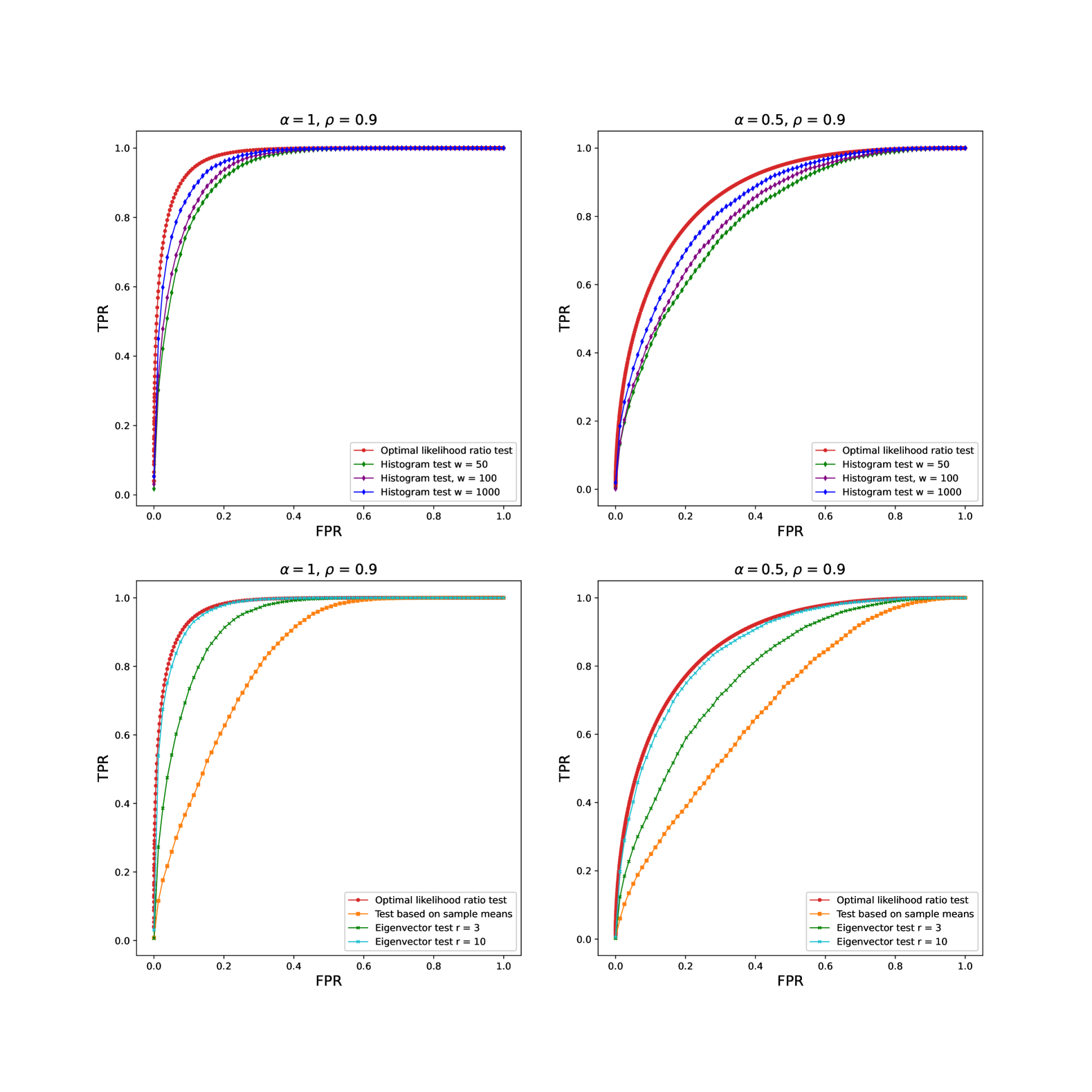
Figure 1: ROC curves of various tests for the broken bivariate Gaussian samples $(d=1)$.

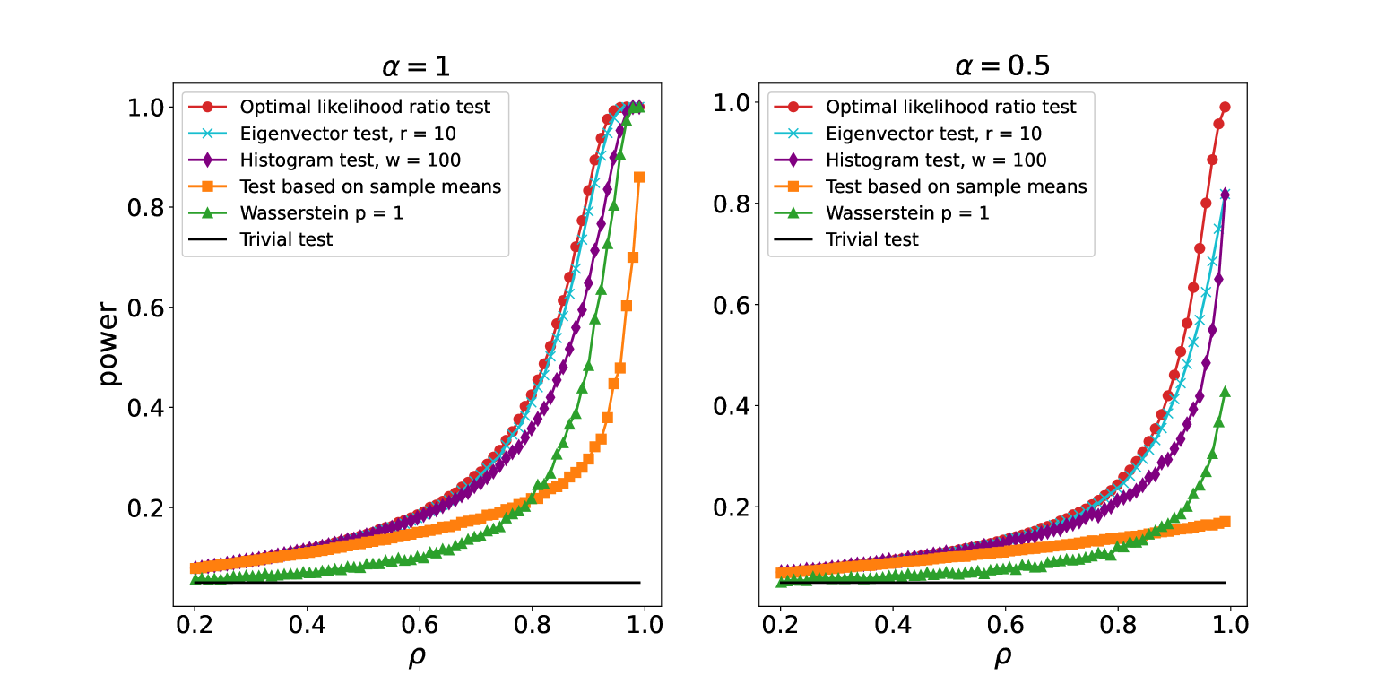
Figure 2: Power curves of various tests for the broken bivariate Gaussian samples $(d=1)$ and Type-I error fixed at 0.05. Left: equal sample sizes $m=n$. Right: unequal sample sizes $m=n/2$.

Power analysis

Next, we compare the asymptotic power ($n=\infty$) of these tests under the Gaussian model in one dimension. The spectral embedding are obtained by applying Hermite polynomials $\phi_{k}=\psi_{k}=\frac{1}{\sqrt{k!}}H_{k}$ for degree up to $r$. For histograms, we use $w$ quantile intervals for the Gaussian distribution as the partition. Fixing $\rho=0.9$ and $\alpha=1$ or $0.5$, Fig. 1 plots the receiver operating characteristic (ROC) curves of the optimal likelihood ratio test, histogram tests for various bin size $w$ (upper panel), and spectral test $T_{\rm{eigen}}$ for various degree $r$ (lower panel). We make two observations:

• First, spectral embedding is much more efficient than histogram embedding, in the sense that the power of the former converges rapidly to the optimal curve as $r$ increases, whereas the latter requires a significantly larger number of bins $w$ to achieve a comparable performance. This can be attributed to exponential decay of eigenvalues in the Gaussian model (cf. (25)) whereas quantization error typically decays polynomially in the quantization level.

• Second, unequal sample sizes are more difficult to test, as a constant proportion of the $X$ sample (of unknown location) is independent of the $Y$ sample, thereby further obscuring the correlation. Indeed, for both spectral and histogram tests, smaller $\alpha$ requires a larger embedding dimension ($r$ or $w$) to achieve a similar accuracy. For the spectral test, the proof of Corollary 2 suggests that $r$ needs to be inversely proportional to $\alpha$ – see (26).

Based on these ROC curves, next we choose $w=100$ for histogram test and $r=10$ for spectral test and plot their power curves. For each test statistic, we choose the threshold so that the Type-I error is fixed at 0.05 and plot the power (one minus Type-II error) against the correlation level $\rho\in[0.2,0.99]$. Also included are the test (16) based on sample means (which is a special case of the spectral test for $r=1$) and the trivial test (rejecting ${\mathcal{H}}_{0}$ with probability $0.05$ independently of the data, with a constant power of $0.05$.)

For equal sample size ($\alpha=1$, left panel of Fig. 2), all tests have power approaching 1 as $\rho\to 1$, including the test based on sample means. However, the performance of degree-10 spectral test is much closer to optimal than that of histogram with 100 bins. For unequal sample size ($\alpha=1/2$, right panel of Fig. 2), all tests have lower power compared to the case of $\alpha=1$. As remarked after Corollary 2, test based solely on sample means fails to achieve power 1 even if $\rho\to 1$ and it is necessary to incorporate higher-order eigenfunctions.

Wasserstein test

Finally, we discuss a natural test statistic based on the Wasserstein distance for identical marginals ${\mathsf{P}}_{X}={\mathsf{P}}_{Y}$. As mentioned in Section 3.2, the empirical distributions $\hat{P}_{X}$ and $\hat{P}_{Y}$ are concentrated on the population, whose fluctuations are independent under ${\mathcal{H}}_{0}$ and correlated under ${\mathcal{H}}_{1}$. As such, it is natural to expect that the typical distance between $\hat{P}_{X}$ and $\hat{P}_{Y}$ tends to be smaller under ${\mathcal{H}}_{1}$ than that under ${\mathcal{H}}_{0}$. This motivates the test which rejects ${\mathcal{H}}_{0}$ if $W_{p}(\hat{P}_{X},\hat{P}_{Y})$, the $p$-Wasserstein distance between these two empirical distributions, is small than a threshold. In the special case of $n=m$, this amounts to solving a linear assignment problem:

$$W_{p}^{p}(\hat{P}_{X},\hat{P}_{Y})=\frac{1}{n}\min_{\pi\in S_{n}}\sum_{i=1}^{n}\|X_{\pi(i)}-Y_{i}\|^{p}.$$ (19)

which, in the case of $p=2$, is the same as the MLE (2). For $p=1$, by the Kantorovich-Rubinstein duality, it can be interpreted as computing the maximum difference between the empirical averages over all $1$-Lipschitz test functions (as opposed to explicit test functions based on spectral or histogram embedding). The Wasserstein test is appealing for two reasons: (a) it is universal without requiring knowledge of the joint distribution; (b) it scales well with the ambient dimension $d$ and can be computed in time $O(n^{2}d+n^{3})$ (first computing the weight matrix and solving the linear assignment). In comparison, how the embedding dimension of histogram or spectral embedding scales with $d$ must be chosen carefully depending on the joint distribution. (For histogram, it will inevitably be exponential.)

The power curves for this test are also shown in Fig. 2 for $n=1000$ and $p=1$ (The curves for $p=2$ are qualitatively similar and omitted for brevity.) As seen in the left panel for equal sample sizes ($\alpha=1$), although for smaller $\rho$ the Wasserstein test underperforms the sample mean test, its power eventually approaches $1$ as $\rho\to 1$. However, its performance remains inferior to the histogram and spectral tests, which more closely approximate the optimal likelihood ratio test. For unequal sample sizes ($\alpha<1$), it is not hard to see that the Wasserstein test fails to achieve strong detection even if $\rho=1$ (as seen in the right panel for $\alpha=0.5$).

4 Proof of lower bounds

Proof of Theorem 1.

We first simplify the expression for

$$\mathbb{E}_{0}{\mathbf{L}}^{2} =\frac{1}{\left|S_{m,n}\right|^{2}}\sum_{\pi,\pi^{\prime}\in S_{m,n}}\mathbb{E}_{0}\left[\prod_{i=1}^{m}L(X_{\pi(i)},Y_{i})L(X_{\pi^{\prime}(i)},Y_{i})\right]$$

$$=\frac{1}{\left|S_{m,n}\right|}\sum_{\pi\in S_{m,n}}\mathbb{E}_{0}\left[\prod_{i=1}^{m}L(X_{\pi(i)},Y_{i})L(X_{i},Y_{i})\right],$$

where the second equality holds by symmetry and setting $\pi^{\prime}(i)=i,\forall i\in[m]$.

For a fixed $\pi$, a key observation is

$$\mathbb{E}_{0}\left[\prod_{i=1}^{m}L(X_{\pi(i)},Y_{i})L(X_{i},Y_{i})\right]=\mathbb{E}_{0}\left[\prod_{i\in I}L(X_{\pi(i)},Y_{i})L(X_{i},Y_{i})\right],$$ (20)

where $I$ is defined as the largest subset of $[m]$ such that $\pi(I)=I$. To see why this equality holds, note that if $X_{j}$ appears only once, say $L(X_{j},Y_{i})$, in the product of $\prod_{i=1}^{m}L(X_{\pi(i)},Y_{i})L(X_{i},Y_{i})$, then $L(X_{j},Y_{i})$ can be eliminated by taking the expectation over $X_{j}$ and using the fact that $\mathbb{E}_{X_{j}}[L(X_{j},Y_{i})]=1$. Therefore, we can eliminate all those $X_{j}$’s that appear only once. Similarly, if there exists $Y_{i}$ appearing only once, say $L(X_{j},Y_{i})$, in the remaining product, then $L(X_{j},Y_{i})$ can be also eliminated by taking the expectation over $Y_{i}$ and using the fact that $\mathbb{E}_{Y_{i}}[L(X_{j},Y_{i})]=1$.

This elimination procedure continues until no $X_{j}$ or $Y_{i}$ can be dropped. The remaining indices are then given by $I\subset[m]$, i.e., all $X_{i}$ and $Y_{i}$ appear exactly twice for $i\in I$. Alternatively, one can view this iterative elimination procedure as finding the $2$-core of a bipartite graph $G_{\pi}$ with left node set $[m]$ and right node set $[n]$ and edge set $\{(i,\pi(i))\}_{i=1}^{m}\cup\{(i,i)\}_{i=1}^{m}$. After successively removing all nodes with degree at most $1$ together with its incident edge, the remaining subgraph is the $2$-core of $G_{\pi}$ and the set of remaining left and right nodes are both $I$. See Fig. 3 for an illustration.

Figure 3: An instance of the bipartite graph $G_{\pi}$ for $n=8$ and $m=6$. The edges $(i,i)$ and $(i,\pi(i))$ are in blue (dashed) and red (solid), respectively. Here, the 2-core is a 6-cycle with $I=\{1,2,3\}$. After removing this 2-core, the remaining graph consists two disjoint paths of lengths 2 and 4.

Note that $\pi$ restricted to $I$, $\pi_{|_{I}}$, is a permutation on $I$. To further compute the RHS of (20), let ${\mathcal{O}}$ denote the set of disjoint cycles of $\pi_{|_{I}}$ and $N_{i}$ denote the number of cycles of length $i$. (Note that the 2-core of $G_{\pi}$ must be a disjoint union of cycles; there are exactly $N_{i}$ cycles of length $i$.) By applying the spectral decomposition, one can obtain

$$\mathbb{E}_{0}\left[\prod_{i\in I}L(X_{\pi(i)},Y_{i})L(X_{i},Y_{i})\right] =\prod_{O\in{\mathcal{O}}}\mathbb{E}_{0}\left[\prod_{i\in O}L(X_{\pi(i)},Y_{i})L(X_{i},Y_{i})\right]$$

$$=\prod_{O\in{\mathcal{O}}}\mathbb{E}_{0}\left[\prod_{i\in O}\sum_{k,k^{\prime}=0}^{\infty}\lambda_{k}\lambda_{k^{\prime}}\phi_{k}(X_{\pi(i)})\phi_{k^{\prime}}(X_{i})\psi_{k}(Y_{i})\psi_{k^{\prime}}(Y_{i})\right]$$

$$\overset{(a)}{=}\prod_{O\in{\mathcal{O}}}\mathbb{E}_{0}\left[\prod_{i\in O}\sum_{k=0}^{\infty}\lambda_{k}^{2}\phi_{k}(X_{\pi(i)})\phi_{k}(X_{i})\right]$$

$$\overset{(b)}{=}\prod_{O\in{\mathcal{O}}}\sum_{k=0}^{\infty}\lambda_{k}^{2|O|}=\prod_{i=1}^{\left|I\right|}\left(\sum_{k=0}^{\infty}\lambda_{k}^{2i}\right)^{N_{i}},$$

where in $(a)$ we take expectation over $Y_{i}$ and apply $\mathbb{E}_{{\mathsf{P}}_{Y}}\psi_{k}(Y_{i})\psi_{k^{\prime}}(Y_{i})=\delta_{kk^{\prime}}$, and in $(b)$, we expand product and apply that $\mathbb{E}_{{\mathsf{P}}_{X}}\phi_{k}(X)\phi_{k^{\prime}}(X)=\delta_{kk^{\prime}}$.

Combining the last three displayed equations gives that

$$\mathbb{E}_{0}{\mathbf{L}}^{2}=\frac{1}{\left|S_{m,n}\right|}\sum_{\pi\in S_{m,n}}\prod_{i=1}^{\left|I\right|}\left(\sum_{k=0}^{\infty}\lambda_{k}^{2i}\right)^{N_{i}}=\frac{1}{\left|S_{m,n}\right|}\sum_{I\subset[m]}\sum_{\sigma\in S_{I}}M(I,\sigma)\prod_{i=1}^{\left|I\right|}\left(\sum_{k=0}^{\infty}\lambda_{k}^{2i}\right)^{N_{i}},$$ (21)

where $M(I,\sigma)$ denotes the number of permutations $\pi$ whose corresponding bipartite graph $G_{\pi}$ has $2$-core given by $I$ and $\pi_{|_{I}}=\sigma$.

To determine $M(I,\sigma)$, recall the bipartite graph formulation. Here the edges in $\{(i,i)\}_{i\in[m]}\cup\{(i,\pi(i)\}_{i\in[I]}$ have already been fixed, and $I$ is the left/right node set of the $2$-core. Therefore, to specify $\pi$, it is equivalent to adding $m-\left|I\right|$ edges between $[m]\setminus I$ and $[n]\setminus I$. Additionally, for $I$ being the $2$-core, after adding those $m-\left|I\right|$ edges, the induced subgraph of $G_{\pi}$ on $([m]\setminus I)\times([n]\setminus I)$ must be a vertex-disjoint collection of paths (cf. Fig. 3). We claim that the number of possible ways to add those $m-\left|I\right|$ edges is

$$M(I,\sigma)=\begin{cases}(n-\left|I\right|-1)(n-\left|I\right|-2)\cdots(n-m),&\left|I\right|<m\\ 1,&\left|I\right|=m,\\ \end{cases}$$ (22)

which only depends on the size of $I$; hence in the following, we denote it by $M_{\left|I\right|}$. To justify this claim, we add edges one by one according to an arbitrary ordering of the left vertices $m\backslash I$. Suppose we have added $t$ edges incident to left vertices $v_{1},\ldots,v_{t}$. The next left vertex $v_{t+1}$ must be paired with either a remaining degree-0 right vertex in $[n]\backslash[m]$ or one of the remaining degree-1 right vertex in $[m]\backslash I$ that is not in the same path as $v_{t+1}$. The total number of such right vertices is $n-|I|-t-1$. From here the claim (22) follows.

Finally, by classifying $I$ according to its size, we obtain that

$$\mathbb{E}_{0}{\mathbf{L}}^{2} =\frac{1}{\left|S_{m,n}\right|}\sum_{I\in[m]}\sum_{\sigma\in S_{I}}M_{\left|I\right|}\prod_{i=1}^{\left|I\right|}\left(\sum_{k=0}^{\infty}\lambda_{k}^{2i}\right)^{N_{i}}$$

$$=\frac{1}{\left|S_{m,n}\right|}\sum_{\ell=0}^{m}\binom{m}{\ell}M_{\ell}\sum_{\sigma\in S_{\ell}}\prod_{i=1}^{\left|I\right|}\left(\sum_{k=0}^{\infty}\lambda_{k}^{2i}\right)^{N_{i}}$$

$$\overset{(c)}{=}\frac{1}{\left|S_{m,n}\right|}\sum_{\ell=0}^{m}\binom{m}{\ell}\ell!M_{\ell}a_{\ell}=\sum_{\ell=0}^{m}t_{\ell}a_{\ell},$$

where $(c)$ follows from Lemma 1 in Appendix A and $t_{\ell}=\frac{\binom{m}{\ell}\ell!M_{\ell}}{\binom{n}{m}m!}$. Observe that

$$\sum_{\ell=0}^{m}t_{\ell}=\frac{\sum_{\ell=0}^{m}\binom{n-\ell-1}{m-\ell}}{\binom{n}{m}}=1,$$

since the numerator counts the subsets of $[n]$ of size $m$ based on the largest element $\ell$ for which the subset contains all elements in $[\ell]$. ∎

Proof of Corollary 1.

Note that

$$t_{\ell}=\frac{m(m-1)\cdots(m-\ell+1)(n-m)}{n(n-1)\cdots(n-\ell)}\leq\left(\frac{m}{n}\right)^{\ell}\frac{n-m}{n-\ell}.$$

Now, consider two following cases separately:

• $m\leq(1-c)n$: We have

  $$\mathbb{E}_{0}{\mathbf{L}}^{2}\leq\sum_{\ell=0}^{m}\left(\frac{m}{n}\right)^{\ell}\frac{n-m}{n-\ell}a_{\ell}\leq\sum_{\ell=0}^{\infty}\left(\frac{m}{n}\right)^{\ell}a_{\ell}=\prod_{k=0}^{\infty}\frac{1}{1-(m/n)\lambda^{2}_{k}},$$

  where the second inequality follows from the nonnegativity of $a_{\ell}\geq 0$ and the last equality applies the definition of $a_{\ell}$. Moreover, since $m\leq(1-c)n$ and $\lambda_{k}\leq\lambda_{0}=1,$

  $$\prod_{k=0}^{\infty}\frac{1}{1-m/n\lambda_{k}^{2}}=\exp\left(\sum_{k=0}^{\infty}-\ln\left(1-\frac{m}{n}\lambda_{k}^{2}\right)\right)\leq\exp\left(\sum_{k=0}^{\infty}\frac{\frac{m}{n}\lambda^{2}_{k}}{1-\frac{m}{n}\lambda_{k}^{2}}\right)\leq\exp\left(\frac{m}{cn}\sum_{k=0}^{\infty}\lambda_{k}^{2}\right),$$

  which is $O(1)$ due to the assumption $\sum_{k=1}^{\infty}\lambda^{2}_{k}\leq Cn/m$.

• When $m=(1-o(1))n$: Assuming $\lambda_{1}\leq 1-c_{1}$ and $\sum_{k=1}^{\infty}\lambda^{2}_{k}\leq C$, we have

  $$\left|\sum_{\ell=0}^{m}t_{\ell}a_{\ell}-\prod_{k=1}^{\infty}(1-\lambda^{2}_{k})^{-1}\right| =\left|\sum_{\ell=0}^{m}t_{\ell}\left(a_{\ell}-\prod_{k=1}^{\infty}(1-\lambda^{2}_{k})^{-1}\right)\right|$$

  $$\leq\sum_{\ell=0}^{m}C^{\prime}t_{\ell}r^{-\ell}\leq C^{\prime}\sum_{\ell=0}^{m}\frac{n-m}{n-\ell}r^{-\ell}=o(1),$$

  where the first equality holds due to $\sum_{\ell=0}^{m}t_{n\ell}=1$; the first inequality applies Lemma 2 in Appendix A, where $r>1$ and $C^{\prime}>0$ are constants only depending on $c_{1},C$; the second inequality holds due to $t_{\ell}\leq(n-m)/(n-\ell)$; and the last equality holds due to the assumption that $m=n-o(n)$.

∎

5 Proof of upper bounds

Proof of Theorem 3.

Consider the test statistic (12), namely

$$T_{\rm{top}}=\left(A-B\right)^{2},\quad A\equiv\frac{1}{\sqrt{n}}\sum_{i=1}^{n}\phi_{1}(X_{i}),\;B\equiv\frac{1}{\sqrt{m}}\sum_{i=1}^{m}\psi_{1}(Y_{i}).$$

Under ${\mathcal{H}}_{0}$, $X_{1},\cdots,X_{n},Y_{1}\cdots,Y_{m}$ are all independent, so

$$\mathbb{P}_{0}\left\{T_{\rm{top}}\leq\tau\right\}=\mathbb{E}_{B}[\mathbb{P}\left\{A\in[B-\sqrt{\tau},B+\sqrt{\tau}]\right\}].$$

It remains to argue that $A$ is anti-concentrated. Since $\mathbb{E}_{{\mathsf{P}}_{X}}[\phi^{2}_{1}(X)]=1$, by the Berry-Esseen inequality, we have for some absolute constant $C$,

$$\sup_{x\in{\mathbb{R}}}|\mathbb{P}\left\{A\leq x\right\}-\Phi(x)|\leq\frac{C\mathbb{E}_{{\mathsf{P}}_{X}}|\phi^{3}_{1}(X)|}{\sqrt{n}},$$

where $\Phi$ is the standard normal CDF. So $\mathbb{P}_{0}\left\{T_{\rm{top}}\leq\tau\right\}\leq C^{\prime}(\sqrt{\tau}+\frac{\mathbb{E}_{{\mathsf{P}}_{X}}|\phi^{3}_{1}(X)|}{\sqrt{n}})$ for some absolute constant $C^{\prime}$.

Under ${\mathcal{H}}_{1}$, by symmetry, we can assume $\pi$ to be identity and then

$$\mathbb{E}_{1}\left[T_{\rm{top}}\right] =\mathbb{E}_{1}(A-B)^{2}$$

$$=\frac{1}{n}\mathbb{E}_{1}\left[\sum_{i=1}^{n}\phi_{1}(X_{i})\right]^{2}+\frac{1}{m}\mathbb{E}_{1}\left[\sum_{i=1}^{m}\psi_{1}(Y_{i})\right]^{2}-\frac{2}{\sqrt{nm}}\sum_{i=1}^{n}\sum_{j=1}^{m}\mathbb{E}_{1}\left[\phi_{1}(X_{i})\psi_{1}(Y_{j})\right]$$

$$=2-\frac{2}{\sqrt{nm}}\sum_{i=1}^{m}\mathbb{E}_{{\mathsf{P}}_{X,Y}}\left[\phi_{1}(X)\psi_{1}(Y)\right]$$

$$=2-2\sqrt{\frac{m}{n}}\lambda_{1}\equiv 2\epsilon.$$

By Markov inequality, $\mathbb{P}_{1}\left\{T_{\rm{top}}\geq\tau\right\}\leq\frac{2\epsilon}{\tau}$. Choosing $\tau=\sqrt{\epsilon}$, we have $\mathbb{P}_{1}\left\{T_{\rm{top}}\geq\tau\right\}+\mathbb{P}_{0}\left\{T_{\rm{top}}\leq\tau\right\}\to 0$ provided that $\epsilon\to 0$ and $\mathbb{E}_{{\mathsf{P}}_{X}}|\phi^{3}_{1}(X)|=o(\sqrt{n})$.

Under condition $\mathbb{E}_{{\mathsf{P}}_{Y}}|\psi^{3}_{1}(Y)|=o(\sqrt{m})$, similar argument applies. ∎

Proof of Theorem 4.

Consider the test statistic (15), namely

$$T_{\rm{inner}}=\frac{1}{\sqrt{mn}}\sum_{i=1}^{n}\sum_{j=1}^{m}L_{r}(X_{i},Y_{j})=\frac{1}{\sqrt{mn}}\sum_{i=1}^{n}\sum_{j=1}^{m}\sum_{k=1}^{r}\lambda_{k}\phi_{k}(X_{i})\psi_{k}(Y_{j}),$$

and the test

$$\eta_{r}=\begin{cases}1,&T_{\rm{inner}}>\frac{\sqrt{\frac{m}{n}}\sum_{k=1}^{r}\lambda_{k}^{2}}{2};\\ 0,&\text{otherwise};\\ \end{cases}.$$

Suppose that for a given choice of $r$ (which may depend on $n$), we have

$$\lim_{n\to\infty}I_{\chi^{2}}^{(r)}(X;Y)=\infty,\quad\mathbb{E}_{{\mathsf{P}}_{X,Y}}L^{2}_{r}(X,Y)=o\left(n(I_{\chi^{2}}^{(r)}(X;Y))^{2}\right).$$

We will first compute $\mathbb{E}_{0}\left[T_{\rm{inner}}\right]$, $\mathbb{E}_{1}\left[T_{\rm{inner}}\right]$, $\mathsf{var}_{0}\left[T_{\rm{inner}}\right]$ and $\mathsf{var}_{1}\left[T_{\rm{inner}}\right]$ and then use Chebyshev’s inequality to show that strong detection is achievable. First, by the orthonormality of $\{\phi_{k}\}_{k\geq 0}$,

$$\mathbb{E}_{0}\left[T_{\rm{inner}}\right]=\frac{1}{\sqrt{mn}}\sum_{i=1}^{n}\sum_{j=1}^{m}\sum_{k=1}^{r}\lambda_{k}\mathbb{E}_{0}[\phi_{k}(X_{i})\psi_{k}(Y_{j})]=0.$$

Moreover, by symmetry, we may set $\pi$ to be identity and then,

$$\mathbb{E}_{1}\left[T_{\rm{inner}}\right]=\frac{1}{\sqrt{mn}}\sum_{i=1}^{m}\sum_{j=1}^{m}\sum_{k=1}^{r}\lambda_{k}\mathbb{E}_{1}\phi_{k}(X_{i})\psi_{k}(Y_{j})=\frac{1}{\sqrt{mn}}\sum_{i=1}^{m}\sum_{k=1}^{r}\lambda_{k}\mathbb{E}_{1}\phi_{k}(X_{i})\psi_{k}(Y_{j})=\sqrt{\frac{m}{n}}\sum_{k=1}^{r}\lambda^{2}_{k},$$

where the second equality holds because when $i\neq j$, $(X_{i},Y_{j})$ is distributed as ${\mathsf{P}}_{X}\otimes{\mathsf{P}}_{Y}$ and $\mathbb{E}_{{\mathsf{P}}_{X}}\left[\phi_{k}(X_{i})\right]=\mathbb{E}_{{\mathsf{P}}_{Y}}\left[\psi_{k}(Y_{j})\right]=0$; the last equality follows because $(X_{i},Y_{i})$ is distributed as ${\mathsf{P}}_{X,Y}$ so that $\mathbb{E}_{1}\left[\phi_{k}(X_{i})\psi_{k}(Y_{i})\right]=\lambda_{k}$.

For $\mathsf{var}_{0}\left[T_{\rm{inner}}\right]$, we have

$$\mathsf{var}_{0}\left[T_{\rm{inner}}\right] =\mathbb{E}_{0}\left[T_{\rm{inner}}^{2}\right]=\frac{1}{nm}\sum_{i,i^{\prime}=1}^{n}\sum_{j,j^{\prime}=1}^{m}\mathbb{E}_{0}\left[L_{r}(X_{i},Y_{j})L_{r}(X_{i^{\prime}},Y_{j^{\prime}})\right]$$

$$=\frac{1}{nm}\sum_{i,i^{\prime}=1}^{n}\sum_{j,j^{\prime}=1}^{m}\mathbb{E}_{0}\left[\sum_{k=1}^{r}\lambda_{k}\phi_{k}(X_{i})\psi_{k}(Y_{j})\sum_{k^{\prime}=1}^{r}\lambda_{k^{\prime}}\phi_{k^{\prime}}(X_{i^{\prime}})\psi_{k^{\prime}}(Y_{j^{\prime}})\right]$$

$$=\frac{1}{nm}\sum_{k,k^{\prime}=1}^{r}\lambda_{k}\lambda_{k^{\prime}}\sum_{i,i^{\prime}=1}^{n}\sum_{j,j^{\prime}=1}^{m}\mathbb{E}\left[\phi_{k}(X_{i})\phi_{k^{\prime}}(X_{i^{\prime}})\right]\mathbb{E}\left[\psi_{k}(Y_{j})\psi_{k^{\prime}}(Y_{j^{\prime}})\right]$$

$$=\frac{1}{nm}\sum_{k,k^{\prime}=1}^{r}\lambda_{k}\lambda_{k^{\prime}}\sum_{i=1}^{n}\sum_{j=1}^{m}\delta_{k,k^{\prime}}=\sum_{k=1}^{r}\lambda_{k}^{2}.$$

For $\mathsf{var}_{1}\left[T_{\rm{inner}}\right]=\mathbb{E}_{1}\left[T_{\rm{inner}}^{2}\right]-(\mathbb{E}_{1}\left[T_{\rm{inner}}\right])^{2}$, we only need to calculate $\mathbb{E}_{1}\left[T_{\rm{inner}}^{2}\right]$, which by symmetry is

$$\mathbb{E}_{1}\left[T_{\rm{inner}}^{2}\right]=\frac{1}{nm}\sum_{i,i^{\prime}=1}^{n}\sum_{j,j^{\prime}=1}^{m}\mathbb{E}_{1|{\rm Id}}\left[L_{r}(X_{i},Y_{j})L_{r}(X_{i^{\prime}},Y_{j^{\prime}})\right].$$

The summands can be divided into five cases:

• $i=j=i^{\prime}=j^{\prime}$: We have

  $$\mathbb{E}_{1|\rm Id}\left[L^{2}_{r}(X_{i},Y_{i})\right]=\mathbb{E}_{{\mathsf{P}}_{X,Y}}\left[L^{2}_{r}(X,Y)\right].$$

• $i=i^{\prime},j=j^{\prime}$ but $i\neq j$:

  $$\mathbb{E}_{1|\rm Id}\left[L_{r}(X_{i},Y_{j})L_{r}(X_{i},Y_{j})\right]=\mathbb{E}_{{\mathsf{P}}_{X}\otimes{\mathsf{P}}_{Y}}\left[L^{2}_{r}(X_{i},Y_{j})\right]=\sum_{k=1}^{r}\lambda_{k}^{2}.$$

• $i=j,i^{\prime}=j^{\prime}$ but $i\neq i^{\prime}$:

  $$\mathbb{E}_{1|\rm Id}\left[L_{r}(X_{i},Y_{i})L_{r}(X_{i^{\prime}},Y_{i^{\prime}})\right]=\left(\mathbb{E}_{{\mathsf{P}}_{X,Y}}\left[L_{r}(X,Y)\right]\right)^{2}=\left(\sum_{k=1}^{r}\lambda_{k}\mathbb{E}_{{\mathsf{P}}_{X,Y}}\left[\phi_{k}(X)\psi_{k}(Y)\right]\right)^{2}=\left(\sum_{k=1}^{r}\lambda_{k}^{2}\right)^{2}.$$

• $i=j^{\prime},i^{\prime}=j$ but $i\neq i^{\prime}$:

  $$\mathbb{E}_{1|\rm Id}\left[L_{r}(X_{i},Y_{j})L_{r}(X_{j},Y_{i})\right]=\sum_{k,k^{\prime}=1}^{r}\lambda_{k}\lambda_{k^{\prime}}\mathbb{E}_{{\mathsf{P}}_{X,Y}}\left[\phi_{k}(X_{i})\psi_{k^{\prime}}(Y_{i})\right]\mathbb{E}_{{\mathsf{P}}_{X,Y}}\left[\phi_{k^{\prime}}(X_{j})\psi_{k}(Y_{j})\right]=\sum_{k=1}^{r}\lambda_{k}^{4}.$$

• In the remaining case, there is at least one isolated index, hence the corresponding summand must be $0$.

We conclude that

$$\mathbb{E}_{1}\left[T_{\rm{inner}}^{2}\right]=\frac{1}{n}\mathbb{E}_{{\mathsf{P}}_{X,Y}}\left[L^{2}_{r}(X,Y)\right]+\frac{n-1}{n}\left(\sum_{k=1}^{r}\lambda_{k}^{2}\right)+\frac{m-1}{n}\left(\sum_{k=1}^{r}\lambda_{k}^{2}\right)^{2}+\frac{m-1}{n}\left(\sum_{k=1}^{r}\lambda_{k}^{4}\right).$$

Therefore,

$$\mathsf{var}_{1}\left[T_{\rm{inner}}\right] =\frac{1}{n}\mathbb{E}_{{\mathsf{P}}_{X,Y}}\left[L^{2}_{r}(X,Y)\right]+\frac{n-1}{n}\left(\sum_{k=1}^{r}\lambda_{k}^{2}\right)-\frac{1}{n}\left(\sum_{k=1}^{r}\lambda_{k}^{2}\right)^{2}+\frac{m-1}{n}\left(\sum_{k=1}^{r}\lambda_{k}^{4}\right)$$

$$\leq\frac{1}{n}\mathbb{E}_{{\mathsf{P}}_{X,Y}}\left[L^{2}_{r}(X,Y)\right]+2\sum_{k=1}^{r}\lambda_{k}^{2},$$

where the last inequality holds due to $\lambda_{k}^{4}\leq\lambda_{k}^{2}$ for all $k\geq 1$ and $m\leq n$.

Then the testing error of $\eta_{r}$ could be bounded from above by

$$\mathbb{P}_{0}\left\{T_{\rm{inner}}>\frac{\sqrt{\frac{m}{n}}\sum_{k=1}^{r}\lambda_{k}^{2}}{2}\right\}+\mathbb{P}_{1}\left\{T_{\rm{inner}}\leq\frac{\sqrt{\frac{m}{n}}\sum_{k=1}^{r}\lambda_{k}^{2}}{2}\right\}$$

$$\leq\frac{4\mathsf{var}_{0}\left[T_{\rm{inner}}\right]}{\frac{m}{n}(I_{\chi^{2}}^{(r)}(X;Y))^{2}}+\frac{4\mathsf{var}_{1}\left[T_{\rm{inner}}\right]}{\frac{m}{n}(I_{\chi^{2}}^{(r)}(X;Y))^{2}}$$

$$\leq\frac{4}{\frac{m}{n}I_{\chi^{2}}^{(r)}(X;Y)}+\frac{4\mathbb{E}_{{\mathsf{P}}_{X,Y}}\left[L^{2}_{r}(X,Y)\right]}{m\left(I_{\chi^{2}}^{(r)}(X;Y)\right)^{2}}+\frac{8}{\frac{m}{n}I_{\chi^{2}}^{(r)}(X;Y)}\to 0,$$

where the first inequality follows from Chebyshev’s inequality and we use that $I_{\chi^{2}}^{(r)}(X;Y)=\sum_{k=1}^{r}\lambda_{k}^{2}$. ∎

Proof of Theorem 2.

The necessity part directly follows from Corollary 1.

For sufficiency, we split the proof into two parts. First, assuming $I_{\chi^{2}}(X;Y)=\infty$, we show that strong detection is achievable for any $0<\alpha\leq 1$. For any fixed $K>0$, by Lemma 5, there exists a partition ${\mathcal{I}}=\{I_{1},I_{2},\cdots,I_{w}\}$ on ${\mathcal{X}}$ and ${\mathcal{J}}=\{J_{1},J_{2},\cdots,J_{w}\}$ on ${\mathcal{Y}}$ such that the induced partition ${\mathcal{E}}=\{I_{k}\times J_{l}\}_{k,l=1}^{w}$ on ${\mathcal{X}}\times{\mathcal{Y}}$ satisfies the following: if we define the discretized joint distributions ${\mathsf{P}}_{\mathcal{E}}(k,l)={\mathsf{P}}_{X,Y}(I_{k}\times J_{l})$ and ${\mathsf{Q}}_{\mathcal{E}}(k,l)={\mathsf{P}}_{X}(I_{k}){\mathsf{P}}_{Y}(J_{l})$, then $\chi^{2}({\mathsf{P}}_{\mathcal{E}}\|{\mathsf{Q}}_{\mathcal{E}})>K$.

Recall the definition of the standardized histograms $s$ and $t$ from (8), namely

$$s_{k}=\frac{1}{\sqrt{n}}\sum_{i=1}^{n}\frac{{\mathbf{1}_{\left\{{X_{i}\in I_{k}}\right\}}}-r_{k}}{\sqrt{r_{k}}},\quad t_{l}=\frac{1}{\sqrt{m}}\sum_{i=1}^{m}\frac{{\mathbf{1}_{\left\{{Y_{i}\in J_{l}}\right\}}}-z_{l}}{\sqrt{z_{l}}},$$

where $r_{k}={\mathsf{P}}_{X}(I_{k})$ for $k\in[w]$ and $z_{l}={\mathsf{P}}_{Y}(J_{l})$ for $l\in[w]$. Under the two hypotheses, the covariance matrices of $(s,t)$ can be computed as follows:

$$\Sigma_{0}=\mathbb{E}_{0}\begin{bmatrix}ss^{\top}&ts^{\top}\\ st^{\top}&tt^{\top}\end{bmatrix}=\begin{bmatrix}A&\mathbf{0}\\ \mathbf{0}&B\end{bmatrix},\quad\Sigma_{1}=\mathbb{E}_{1}\begin{bmatrix}ss^{\top}&ts^{\top}\\ st^{\top}&tt^{\top}\end{bmatrix}=\begin{bmatrix}A&\sqrt{\alpha}C\\ \sqrt{\alpha}C^{\top}&B\end{bmatrix},$$

where

$$A=\mathbf{I}_{w}-\gamma\gamma^{\top},B=\mathbf{I}_{w}-\beta\beta^{\top},C={\widetilde{P}}-\gamma\beta^{\top}.$$

Here $\gamma=(\sqrt{r_{1}},\sqrt{r_{2}},\cdots,\sqrt{r_{w}})^{\top}$ and $\beta=(\sqrt{z_{1}},\sqrt{z_{2}},\cdots,\sqrt{z_{w}})^{\top}$ are both unit vectors, and ${\widetilde{P}}_{k,l}\equiv{\mathsf{P}}_{X,Y}(I_{k}\times J_{l})/\sqrt{r_{k}z_{l}}$. Note that both $\Sigma_{0}$ and $\Sigma_{1}$ have zero eigenvalues because the entries of $s$ and $t$ are linearly dependent. To resolve this rank deficiency, we first project $(s,t)$ to the space spanned by eigenvectors of $\Sigma_{0}$ corresponding to non-zero eigenvalues.

Importantly, the left (resp. right) singular vectors of the off-diagonal block $C$ coincide with those of the diagonal block $A$ (resp. $B$). Indeed, one can verify that $C^{\top}\gamma=\mathbf{0}$ and $C\beta=\mathbf{0}$. Assume the singular value decomposition of $C$ is $C=U\Lambda V^{\top}$, where $U,V$ are orthogonal matrices in the form of $U=({\widetilde{U}},\gamma)$ and $V=({\widetilde{V}},\beta)$ and $\Lambda=\mathsf{diag}\left\{{\mu_{1},\mu_{2},\cdots,\mu_{w}}\right\}$ with $1\geq\mu_{1}\geq\mu_{2}\geq\cdots\geq\mu_{w}=0$. (These are in fact singular values of the discretized likelihood operator.)

Define the diagonal matrix $\widetilde{\Lambda}={\widetilde{U}}^{\top}C{\widetilde{V}}=\mathsf{diag}\left\{{\mu_{1},\cdots,\mu_{w-1}}\right\}$. Let $\tilde{s}={\widetilde{U}}^{\top}s$ and $\tilde{t}={\widetilde{V}}^{\top}t$, whose covariance matrices are

$$\widetilde{\Sigma}_{0}=\mathbf{I}_{2w-2},\quad\widetilde{\Sigma}_{1}=\begin{bmatrix}\mathbf{I}_{w-1}&{\sqrt{\alpha}}\widetilde{\Lambda}\\ {\sqrt{\alpha}}\widetilde{\Lambda}^{\top}&\mathbf{I}_{w-1}\end{bmatrix}.$$

Consider two cases:

Case I: $\mu_{1}=1$ and $\alpha=1$. In this case, under ${\mathcal{H}}_{1}$, $\tilde{s}_{1}=\tilde{t}_{1}$ with probability 1. Under ${\mathcal{H}}_{0}$, by CLT, $\tilde{s}_{1}-\tilde{t}_{1}\to{\mathcal{N}}(0,2)$ weakly as $n\to\infty$. Thus the test ${\mathbf{1}_{\left\{{\tilde{s}_{1}=\tilde{t}_{1}}\right\}}}$ attains vanishing probability of error.

Case II: $\mu_{1}<1$ or $\alpha<1$. As a result, $\widetilde{\Sigma}_{1}$ is invertible, with eigenvalues $1\pm\sqrt{\alpha}\mu_{k}$. By CLT, as $n\to\infty$, $(\tilde{s},\tilde{t})^{\top}$ converges to ${\mathsf{N}}_{0}\triangleq{\mathcal{N}}(\mathbf{0},\widetilde{\Sigma}_{0})$ and ${\mathsf{N}}_{1}\triangleq{\mathcal{N}}(\mathbf{0},\widetilde{\Sigma}_{1})$ under ${\mathcal{H}}_{0}$ and ${\mathcal{H}}_{1}$, respectively. Consider the likelihood ratio test ${\mathbf{1}_{\left\{{T>0}\right\}}}$ under the normal limits, where

$$T=-\begin{pmatrix}\tilde{s}\\ \tilde{t}\end{pmatrix}^{\top}\left(\widetilde{\Sigma}_{1}^{-1}-\mathbf{I}_{2w-2}\right)\begin{pmatrix}\tilde{s}\\ \tilde{t}\end{pmatrix}-\sum_{k=1}^{w}\log(1-\alpha\mu_{k}^{2}).$$

By weak convergence, $\mathbb{P}_{0}[T>0]=\mathbb{P}_{{\mathsf{N}}_{0}}[T>0]+o_{n}(1)$ and $\mathbb{P}_{1}[T\leq 0]=\mathbb{P}_{{\mathsf{N}}_{1}}[T\leq 0]+o_{n}(1)$. Thus it remains to bound $\mathbb{P}_{{\mathsf{N}}_{0}}[T>0]+\mathbb{P}_{{\mathsf{N}}_{1}}[T\leq 0]=1-\mathrm{TV}({\mathsf{N}}_{0},{\mathsf{N}}_{1})$.

To this end, recall that $\mu_{k}$ is the singular value of $C$. Consequently,

$$\sum_{k=1}^{w}\mu_{k}^{2}=\mathsf{Tr}\left(C^{\top}C\right)=\mathsf{Tr}\left({\widetilde{P}}^{\top}{\widetilde{P}}-{\widetilde{P}}^{\top}\gamma\beta^{\top}-\beta\gamma^{\top}{\widetilde{P}}+\beta\gamma^{\top}\gamma\beta^{\top}\right)=\mathsf{Tr}({\widetilde{P}}^{\top}{\widetilde{P}})-1.$$

By definition of ${\mathsf{P}}_{\mathcal{E}}$ and ${\mathsf{Q}}_{\mathcal{E}}$, we have

$$\mathsf{Tr}\left({\widetilde{P}}^{\top}{\widetilde{P}}\right)=\sum_{k=1}^{w}\sum_{l=1}^{w}\frac{{\mathsf{P}}_{X,Y}^{2}(I_{k}\times J_{l})}{r_{k}z_{l}}=\sum_{k,l}\frac{{\mathsf{P}}_{X,Y}^{2}(I_{k}\times J_{l})}{{\mathsf{P}}_{X}\otimes{\mathsf{P}}_{Y}(I_{k}\times J_{l})}=\sum_{k,l}\frac{{\mathsf{P}}^{2}_{\mathcal{E}}(k,l)}{{\mathsf{Q}}_{\mathcal{E}}(k,l)}=\chi^{2}({\mathsf{P}}_{\mathcal{E}}\|{\mathsf{Q}}_{\mathcal{E}})+1.$$

Then $\sum_{k=1}^{w-1}\mu_{k}^{2}=\chi^{2}({\mathsf{P}}_{\mathcal{E}}\|{\mathsf{Q}}_{\mathcal{E}})>K$ by choice of the partition. The total variation can then be bounded via Hellinger distance as follows:

$$1-\mathrm{TV}({\mathsf{N}}_{0},{\mathsf{N}}_{1})\leq 1-\frac{H^{2}({\mathsf{N}}_{0},{\mathsf{N}}_{1})}{2}=\frac{{\rm det}\left(\widetilde{\Sigma}_{0}\widetilde{\Sigma}_{1}\right)^{1/4}}{{\rm det}\left(\frac{\widetilde{\Sigma}_{0}+\widetilde{\Sigma}_{1}}{2}\right)^{1/2}} =\left\{\prod_{k=1}^{w-1}\frac{1-\alpha\mu_{k}^{2}}{(1-\alpha\mu_{k}^{2}/4)^{2}}\right\}^{1/4}$$

$$\leq\exp\left(-\frac{\alpha}{8}\sum_{k=1}^{w-1}\mu_{k}^{2}\right)\leq\exp\left(-\frac{\alpha K}{8}\right),$$ (23)

where the first equality applies the Hellinger distance between two Gaussians ([28, Sec. 7.7]) and the second inequality holds due to $(1-x)/(1-x/4)^{2}\leq 1-x/2\leq\exp(-x/2)$. The proof is complete by the arbitrariness of $K$.

Finally, assume $\alpha=1$, $I_{\chi^{2}}(X;Y)<\infty$ and $\rho(X;Y)=\lambda_{1}=1$. Consider the same test used in proving Theorem 3. Note that ${\mathsf{P}}_{X,Y}$ is a fixed distribution. Hence, the third-moment condition in Theorem 3 automatically holds, and $T_{\rm{top}}$ achieves strong detection when $\rho(X;Y)=1$.

∎

6 Discussion and open problems

In this paper, we address the problem of testing dependency between two datasets with missing correspondence. For a fixed joint distribution ${\mathsf{P}}_{X,Y}$ and the sample sizes $m=\alpha n$ for a constant $\alpha\in(0,1]$, we establish that strong detection is possible if and only if the $\chi^{2}$-information $I_{\chi^{2}}(X;Y)=\chi^{2}({\mathsf{P}}_{X,Y}\|{\mathsf{P}}_{X}\otimes{\mathsf{P}}_{Y})$ is infinity, or the maximal correlation $\rho(X;Y)$ equals $1$ and $\alpha=1$, thereby resolving Bai-Hsing’s conjecture positively. We further extend the results to more general settings where ${\mathsf{P}}_{X,Y}$ or the ambient dimension $d$ may depend on $n$. These general results determine the sharp detection thresholds for Gaussian or Bernoulli models in both low and high dimensions, closing gaps in the existing literature.

We close the paper by discussing several open problems.

• Highly unbalanced sample sizes: In certain practical scenarios, one dataset can be much bigger than the other. For example, one of the deanonymization experiments carried out in [25, Section 5] involves the Netflix and IMDb datasets of size $n=480{,}189$ and $m=50$, respectively. As discussed in Remark 4, when $m=o(n)$, the detection threshold is open even for Gaussian models in both low and high dimensions. Letting $\alpha=m/n\to 0$, for fixed $d$, Corollary 1 yields the impossibility condition of $1-\rho^{2}=\Omega(\alpha^{1/d})$ and our general results fail to yield any non-trivial upper bound. For growing $d$, there is a significant gap between the negative result of $\rho^{2}\leq\frac{1}{d}\log\frac{C}{\alpha}$ and positive result $\rho^{2}\gg\frac{1}{d\alpha}$.

• Adapting to the joint distribution: The theory and methods developed in this paper assumed that the joint distribution ${\mathsf{P}}_{X,Y}$ is known, which may not be a practical assumption. To this end, for equal sample sizes, a promising proposal is the Wasserstein test (19) discussed in Section 3.4, based on the intuition that the two empirical distributions are close for correlated samples and far for independent samples. This test is both universal (adapting to the unknown ${\mathsf{P}}_{X,Y}$), computationally appealing (scaling favorably with the dimension), and has strong empirical performance. Identifying the distribution class for which the Wasserstein test attains the optimal detection threshold is an interesting open question.

  In a companion paper [18], we explore the challenging setting of unknown ${\mathsf{P}}_{X,Y}$ in the context of shuffled linear regression, where ${\mathsf{P}}_{X,Y}$ is determined by $Y=\rho\left\langle X,\beta\right\rangle+\sqrt{1-\rho^{2}}Z$ with Gaussian covariates $X\sim{\mathcal{N}}(0,\mathbf{I}_{d})$, Gaussian noise $Z\sim{\mathcal{N}}(0,1)$, and $\beta$ being the unknown regression coefficients uniformly distributed on the unit sphere. In this model, both the construction and the analysis of the tests require new ideas.

Appendix A Auxiliary lemmas

Lemma 1.

Let $N_{i}$ denote the number of $i$-cycles in $\sigma\in S_{\ell}$ for $i\in[\ell]$. Then

$$\frac{1}{\ell!}\sum_{\sigma\in S_{\ell}}\prod_{i=1}^{\ell}\left(\sum_{k=0}^{\infty}\lambda_{k}^{2i}\right)^{N_{i}}=a_{\ell},$$

where $a_{\ell}=[z^{\ell}]\prod_{k=0}^{\infty}1/(1-z\lambda^{2}_{k})$ is the $\ell$-th coefficient in the power series.

Proof.

Note that the left hand side is exactly the cycle index of the permutation group $S_{\ell}$ evaluated at $(\sum_{k=0}^{\infty}\lambda_{k}^{2},\sum_{k=0}^{\infty}\lambda_{k}^{4},\cdots)$. Applying Pólya’s Theorem [32, Theorem 7.7] to group $S_{\ell}$ yields

$$\frac{1}{\ell!}\sum_{\sigma\in S_{\ell}}\prod_{i=1}^{\ell}\left(\sum_{k=0}^{\infty}\lambda_{k}^{2i}\right)^{N_{i}}=\sum_{i_{1}+i_{2}+\cdots=\ell}(\lambda_{1}^{2})^{i_{1}}(\lambda_{2}^{2})^{i_{2}}\cdots=[z^{\ell}]\prod_{k=0}^{\infty}\frac{1}{1-z\lambda_{k}^{2}}=a_{\ell},$$

where the penultimate equality follows from expanding each term inside the product as a geometric sum. ∎

Lemma 2.

If $\lambda_{1}\leq 1-c$ and $\sum_{k=1}^{\infty}\lambda^{2}_{k}\leq C$ for two constants $c\in(0,1)$ and $C>0$, then

$$\left|a_{\ell}-\prod_{k=1}^{\infty}\frac{1}{1-\lambda^{2}_{k}}\right|\leq\frac{C^{\prime}}{r^{\ell}},$$

where $r>1$ and $C^{\prime}>0$ are two constants depending on $c$ and $C$.

Proof.

Let $f(z)\triangleq\prod_{k=0}^{\infty}\frac{1}{1-z\lambda_{k}^{2}}=\sum_{k=0}^{\infty}a_{k}z^{k}$ and define $g(z)=\prod_{k=1}^{\infty}\frac{1}{1-z\lambda_{k}^{2}}=(1-z)f(z)$. Under the given conditions, $\lambda^{2}_{1}\leq c^{\prime}\equiv(1-c)^{2}<1$. We can then fix $r\in(1,\frac{1}{c^{\prime}})$ which satisfies $r\lambda_{1}^{2}\leq rc^{\prime}<1$. Consider integral

$$I=\frac{1}{2\pi\textbf{i}}\oint_{|z|=r}\frac{1}{z^{\ell+1}}f(z){\rm d}z=\frac{1}{2\pi\textbf{i}}\oint_{|z|=r}\frac{1}{z^{\ell+1}}\frac{1}{1-z}g(z){\rm d}z,$$

where the orientation is counterclockwise. Note that the integrand $G(z)\equiv\frac{1}{z^{\ell+1}}\frac{1}{1-z}g(z)$ has two singularities $0$ and $1$ inside the contour. Applying the residue theorem yields

$$I=\text{Res}(G,0)+\text{Res}(G,1)=\frac{\left(\frac{g(z)}{1-z}\right)^{(\ell)}\big{|}_{z=0}}{\ell!}-\left(\frac{g(z)}{z^{\ell+1}}\right)\Big{|}_{z=1}=a_{\ell}-g(1)=a_{\ell}-\prod_{k=1}^{\infty}\frac{1}{1-\lambda_{k}^{2}}.$$

Furthermore,

$$|I|\leq\frac{1}{2\pi}\oint_{|z|=r}\frac{1}{|z^{\ell+1}|}\frac{1}{|1-z|}|g(z)|{\rm d}z\leq\frac{1}{2\pi}\frac{1}{r^{\ell+1}(r-1)}\prod_{k=1}^{\infty}\frac{1}{1-r\lambda_{k}^{2}}\cdot 2\pi r=\frac{1}{r^{\ell}(r-1)}\prod_{k=1}^{\infty}\frac{1}{1-r\lambda_{k}^{2}}.$$

Here $r>1$ and

$$\prod_{k=1}^{\infty}\frac{1}{1-r\lambda_{k}^{2}}=\exp\left(\sum_{k=1}^{\infty}-\ln(1-r\lambda_{k}^{2})\right)\leq\exp\left(\sum_{k=1}^{\infty}\frac{r}{1-r\lambda_{k}^{2}}\lambda_{k}^{2}\right)\leq\exp\left(\frac{rC}{1-rc^{\prime}}\right),$$

As a result,

$$\left|a_{\ell}-\prod_{k=1}^{\infty}\frac{1}{1-\lambda_{k}^{2}}\right|\leq\frac{1}{r^{\ell}(r-1)}\exp\left(\frac{rC}{1-rc^{\prime}}\right)=\frac{C^{\prime}}{r^{\ell}},$$

where $C^{\prime}\triangleq\frac{\exp\left(rC/(1-rc^{\prime})\right)}{r-1}$.

∎

Lemma 3.

Let

$$f(\rho,q)=1-\sqrt{(1-q)^{3}(1-q+\rho q)}-2\sqrt{q^{2}(1-q)^{2}(1-\rho)}-\sqrt{q^{3}(q+\rho(1-q))},$$

where $q\equiv q(n)\in(0,1)$ and $\rho\equiv\rho(n)\in(-\min\{\frac{1-q}{q},\frac{q}{1-q}\},1)$.

1. If $q=o(1)$, then

   $$f(\rho,q)=O(q).$$

2. If $q=o(1)$, $\rho=o(1)$ and $\frac{\left|\rho\right|}{q}\to\infty$, then

   $$f(\rho,q)=O(\left|\rho\right|q),$$

Proof.

1. By Taylor expansion,

   $$(1-q)^{\frac{3}{2}}=1-\frac{3}{2}q+o(q),\quad(1-q+\rho q)^{\frac{1}{2}}=1-\frac{1-\rho}{2}q+o(q),$$

   implying that

   $$\sqrt{(1-q)^{3}(1-q+\rho q)}=1-2q+\frac{\rho q}{2}+o(q).$$

   Then

   $$f(\rho,q)\leq 1-\sqrt{(1-q)^{3}(1-q+\rho q)}=2q-\frac{\rho q}{2}+o(q)=O(q).$$

2. By Taylor expansion, we have

   $$(1-q)^{\frac{3}{2}}=1-\frac{3}{2}q+o(q)=1-\frac{3}{2}q+o(\left|\rho\right|q),$$

   where the last equality follows from our assumption $\frac{\left|\rho\right|}{q}\to\infty$ and high order terms have order at least $2$.

   Similarly,

   $$(1-q+\rho q)^{\frac{1}{2}}=1-\frac{1-\rho}{2}q+o(\left|\rho\right|q),$$

   hence

   $$\sqrt{(1-q)^{3}(1-q+\rho q)}=1-2q+\frac{\rho q}{2}+o(\left|\rho\right|q).$$

   By the same argument,

   $$2\sqrt{q^{2}(1-q)^{2}(1-\rho)}=2q(1-q)\left(1-\frac{1}{2}\rho+o(\left|\rho\right|)\right)=2q-\rho q+o(\left|\rho\right|q).$$

   Consequently,

   $$f(\rho,q)\leq 1-\sqrt{(1-q)^{3}(1-q+\rho q)}-2\sqrt{q^{2}(1-q)^{2}(1-\rho)}=\frac{\rho q}{2}+o(\left|\rho\right|q)=O(\left|\rho\right|q),$$

   where $\rho$ must be positive otherwise condition $\left|\rho\right|/q\to\infty$ cannot hold.

∎

Lemma 4.

Let ${\mathsf{P}},{\mathsf{Q}}$ be two probability measures on ${\mathcal{X}}$ with a $\sigma$-algebra ${\mathcal{F}}$. Given a finite ${\mathcal{F}}$-measurable partition ${\mathcal{E}}=\{E_{1},E_{2},\cdots,E_{n}\}$, define the distribution ${\mathsf{P}}_{\mathcal{E}}$ on $[n]$ by ${\mathsf{P}}_{\mathcal{E}}(i)={\mathsf{P}}(E_{i})$ and ${\mathsf{Q}}_{\mathcal{E}}(i)={\mathsf{Q}}(E_{i})$. Then we have

$$\chi^{2}({\mathsf{P}}\|{\mathsf{Q}})=\sup_{{\mathcal{E}}}\chi^{2}({\mathsf{P}}_{\mathcal{E}}\|{\mathsf{Q}}_{\mathcal{E}}),$$

where the supremum is over all finite ${\mathcal{F}}$-measurable partitions ${\mathcal{E}}$.

Proof.

See [28, Theorem 7.6]. ∎

Lemma 5.

Let ${\mathsf{P}},{\mathsf{Q}}$ be two probability measures on ${\mathcal{X}}\times{\mathcal{Y}}$ with $\sigma$-algebra ${\mathcal{F}}_{\mathcal{X}}\otimes{\mathcal{F}}_{\mathcal{Y}}$. Given a finite ${\mathcal{F}}_{\mathcal{X}}$-measurable partition of ${\mathcal{X}}$ as ${\mathcal{I}}=\{I_{1},I_{2},\cdots,I_{w}\}$ and a finite ${\mathcal{F}}_{\mathcal{Y}}$-measurable partition of ${\mathcal{Y}}$ as ${\mathcal{J}}=\{J_{1},J_{2},\cdots,J_{w}\}$ (without loss of generality, we assume the number of partitions on ${\mathcal{X}}$ and ${\mathcal{Y}}$ are same), they induce a partition on ${\mathcal{X}}\times{\mathcal{Y}}$ as ${\mathcal{E}}=\{I_{k}\times J_{l}\}_{k,l=1}^{w}$. Define the distribution ${\mathsf{P}}_{\mathcal{E}}$ on $\{(k,l)\}_{k,l=1}^{w}$ by ${\mathsf{P}}_{\mathcal{E}}(k,l)={\mathsf{P}}(I_{k}\times J_{l})$ and ${\mathsf{Q}}_{\mathcal{E}}(k,l)={\mathsf{Q}}(I_{k}\times J_{l})$. Then we have

$$\chi^{2}({\mathsf{P}}\|{\mathsf{Q}})=\sup_{{\mathcal{E}}}\chi^{2}({\mathsf{P}}_{\mathcal{E}}\|{\mathsf{Q}}_{\mathcal{E}}),$$

where the supremum is over all possible partition ${\mathcal{E}}$ induced by finite ${\mathcal{F}}_{\mathcal{X}}$-measurable partition ${\mathcal{I}}$ and finite ${\mathcal{F}}_{\mathcal{Y}}$-measurable partition ${\mathcal{J}}$.

Proof.

By Lemma 4, $\chi^{2}({\mathsf{P}}\|{\mathsf{Q}})=\sup_{{\mathcal{G}}}\chi^{2}({\mathsf{P}}_{\mathcal{G}}\|{\mathsf{Q}}_{\mathcal{G}})$, where the supremum is over all finite ${\mathcal{F}}_{{\mathcal{X}}}\otimes{\mathcal{F}}_{{\mathcal{Y}}}$-measurable partition ${\mathcal{G}}$. Thus it suffices to show that we can restrict the supremum to be over all rectangles that are Cartesian product of ${\mathcal{F}}_{\mathcal{X}}$-measurable partition ${\mathcal{I}}$ and finite ${\mathcal{F}}_{\mathcal{Y}}$-measurable partition ${\mathcal{J}}$. This is known for mutual information (see, e.g., [28, (4.29)]) and we next show it also holds for $\chi^{2}$-information.

To this end, fix a partition ${\mathcal{G}}=\{G_{1},G_{2},\cdots,G_{n}\}$. Let ${\mathsf{P}}_{\mathcal{G}}(i)={\mathsf{P}}(G_{i})$ and ${\mathsf{Q}}_{\mathcal{G}}(i)={\mathsf{Q}}(G_{i})$. Fix a constant $\epsilon>0$, we construct a partition ${\mathcal{E}}$ induced by partitions on ${\mathcal{X}}$ and ${\mathcal{Y}}$ such that $\chi^{2}({\mathsf{P}}_{\mathcal{E}}\|{\mathsf{Q}}_{\mathcal{E}})\geq\chi^{2}({\mathsf{P}}_{\mathcal{G}}\|{\mathsf{Q}}_{\mathcal{G}})-\epsilon$.

Fix any $\delta>0$ and $a=\frac{1}{2^{n}}$, one can find ${\widetilde{G}}_{1}$ such that $({\mathsf{P}}+{\mathsf{Q}})(G_{1}\Delta{\widetilde{G}}_{1})<a\delta$, where ${\widetilde{G}}_{1}$ is a finite union of measurable rectangles (see [34, Exercise 1.4.28]), and $\Delta$ denotes symmetric difference. Similarly, one can find $G_{2}^{*}$ which is also a finite union of measurable rectangles such that $({\mathsf{P}}+{\mathsf{Q}})(G_{2}^{*}\Delta G_{2})<a\delta$. Then define ${\widetilde{G}}_{2}=G_{2}^{*}\setminus{\widetilde{G}}_{1}$ and observe that

$$G_{2}\Delta{\widetilde{G}}_{2}=({\widetilde{G}}_{2}\setminus G_{2})\cup(G_{2}\setminus{\widetilde{G}}_{2})\subset(G_{2}^{*}\setminus G_{2})\cup((G_{2}\setminus G_{2}^{*})\cup(G_{2}\cap{\widetilde{G}}_{1}))\subset(G_{2}^{*}\Delta G_{2})\cup(G_{2}\cap{\widetilde{G}}_{1}).$$

Since $G_{1}\cap G_{2}=\emptyset$, we have $G_{2}\cap{\widetilde{G}}_{1}\subset{\widetilde{G}}_{1}\Delta G_{1}$. Consequently, $G_{2}\Delta{\widetilde{G}}_{2}\subset(G_{2}^{*}\Delta G_{2})\cup({\widetilde{G}}_{1}\Delta G_{1})$, and hence $({\mathsf{P}}+{\mathsf{Q}})(G_{2}\Delta{\widetilde{G}}_{2})\leq a\delta+a\delta=2a\delta$.

Repeat the above process and obtain ${\widetilde{G}}_{1},{\widetilde{G}}_{2},\cdots,{\widetilde{G}}_{n-1}$ such that they are mutually disjoint and satisfy $({\mathsf{P}}+{\mathsf{Q}})(G_{k}\Delta{\widetilde{G}}_{k})\leq 2^{k-1}a\delta$ for $k\in[n-1]$. Finally define ${\widetilde{G}}_{n}=({\mathcal{X}}\times{\mathcal{Y}})\setminus({\widetilde{G}}_{1}\cup{\widetilde{G}}_{2}\cdots\cup{\widetilde{G}}_{n-1})$. One can check that $G_{n}\Delta{\widetilde{G}}_{n}\subset(G_{1}\Delta{\widetilde{G}}_{1})\cup\cdots\cup(G_{n-1}\Delta{\widetilde{G}}_{n-1})$ and $({\mathsf{P}}+{\mathsf{Q}})(G_{n}\Delta{\widetilde{G}}_{n})\leq(2^{n}-1)a\delta<\delta$.

Note that the difference between two finite unions of measurable rectangles is still a finite union of measurable rectangles. Therefore, $\widetilde{{\mathcal{G}}}=\{{\widetilde{G}}_{1},{\widetilde{G}}_{2},\cdots,{\widetilde{G}}_{n}\}$ is a partition of ${\mathcal{X}}\times{\mathcal{Y}}$ and each of them is a finite union of measurable rectangles satisfying $({\mathsf{P}}+{\mathsf{Q}})({\widetilde{G}}_{k}\Delta G_{k})<\delta$ for $k\in[n]$. Denote ${\widetilde{G}}_{k}=\cup_{i=1}^{m_{k}}A_{i}^{(k)}\times B_{i}^{(k)}$ for $k\in[n]$, where $A_{i}^{(k)}\in{\mathcal{F}}_{\mathcal{X}}$, $B_{i}^{(k)}\in{\mathcal{F}}_{\mathcal{Y}}$, and $A_{i}^{(k)}\times B_{i}^{(k)}$ are disjoint across different $i$.

For each $k\in[n]$, there exists $\delta_{k}$ such that if $\delta<\delta_{k}$, then

$$\frac{{\mathsf{P}}^{2}(G_{k})}{{\mathsf{Q}}(G_{k})}\leq\frac{({\mathsf{P}}(G_{k})-\delta)^{2}}{{\mathsf{Q}}(G_{k})+\delta}+\frac{\epsilon}{n}\leq\frac{{\mathsf{P}}^{2}({\widetilde{G}}_{k})}{{\mathsf{Q}}({\widetilde{G}}_{k})}+\frac{\epsilon}{n}.$$

Thus if $\delta<\min_{k\in[n]}\delta_{k},$ then

$$\chi^{2}({\mathsf{P}}_{\mathcal{G}}\|{\mathsf{Q}}_{\mathcal{G}})=\sum_{k=1}^{n}\frac{{\mathsf{P}}^{2}(G_{k})}{{\mathsf{Q}}(G_{k})}-1\leq\epsilon+\sum_{k=1}^{n}\frac{{\mathsf{P}}^{2}({\widetilde{G}}_{k})}{{\mathsf{Q}}({\widetilde{G}}_{k})}-1=\epsilon+\chi^{2}({\mathsf{P}}_{\widetilde{{\mathcal{G}}}}\|{\mathsf{Q}}_{\widetilde{{\mathcal{G}}}}).$$

Let ${\mathcal{M}}=\left\{A_{i}^{(k)}\times B_{i}^{(k)}:1\leq i\leq m_{k},1\leq k\leq n\right\}$ denote the partition on ${\mathcal{X}}\times{\mathcal{Y}}$ with only measurable rectangles. Consider a channel which maps $(i,k)$ to $k$. If the input follows distribution ${\mathsf{P}}_{{\mathcal{M}}}$ (resp. ${\mathsf{Q}}_{{\mathcal{M}}}$), then the output follows distribution ${\mathsf{P}}_{\widetilde{{\mathcal{G}}}}$ (resp. ${\mathsf{Q}}_{\widetilde{{\mathcal{G}}}}$). By the data processing inequality for chi-squared divergence (see e.g. [28, Theorem 7.4]), we have

$$\chi^{2}({\mathsf{P}}_{\widetilde{{\mathcal{G}}}}\|{\mathsf{Q}}_{\widetilde{{\mathcal{G}}}})\leq\chi^{2}({\mathsf{P}}_{\mathcal{M}}\|{\mathsf{Q}}_{\mathcal{M}}).$$ (24)

Combining it with the last displayed equation yields that

$$\chi^{2}({\mathsf{P}}_{\mathcal{G}}\|{\mathsf{Q}}_{\mathcal{G}})\leq\chi^{2}({\mathsf{P}}_{\mathcal{M}}\|{\mathsf{Q}}_{\mathcal{M}})+\epsilon.$$

Note that ${\mathcal{M}}$ may not be induced by partitions on ${\mathcal{X}}$ and ${\mathcal{Y}}$. Thus, we define

$${\mathcal{I}}=\left\{\cap_{k=1}^{n}\cap_{i=1}^{m_{k}}C_{i}^{(k)}:C_{i}^{(k)}\in\left\{A_{i}^{(k)},\left(A_{i}^{(k)}\right)^{\rm c}\right\}\right\},$$

and relabel elements of ${\mathcal{I}}$ to be $\{I_{1},I_{2},\cdots,I_{w}\}$. Sets in ${\mathcal{I}}$ are disjoint and $\cup_{k=1}^{w}I_{k}={\mathcal{X}}$; hence ${\mathcal{I}}$ is a partition of ${\mathcal{X}}$. Similarly, define

$${\mathcal{J}}=\left\{\cap_{k=1}^{n}\cap_{i=1}^{m_{k}}D_{i}^{(k)}:D_{i}^{(k)}\in\left\{B_{i}^{(k)},\left(B_{i}^{(k)}\right)^{\rm c}\right\}\right\},$$

and relabel elements of ${\mathcal{J}}$ to be $\{J_{1},J_{2},\cdots,J_{w}\}$, so that ${\mathcal{J}}$ is a partition of ${\mathcal{Y}}$. Let ${\mathcal{E}}=\{I_{k}\times J_{l}\}_{k,l=1}^{w}$. Note that for any $A_{i}^{(k)}\times B_{i}^{(k)}\in{\mathcal{M}}$, $A_{i}^{(k)}$ must be the union of some disjoint elements in ${\mathcal{I}}$, and so is $B_{i}^{(k)}$. Then $A_{i}^{(k)}\times B_{i}^{(k)}$ is a union of disjoint elements in ${\mathcal{E}}$. Therefore, analogous to (24), we can show that

$$\chi^{2}({\mathsf{P}}_{\mathcal{M}}\|{\mathsf{Q}}_{\mathcal{M}})\leq\chi^{2}({\mathsf{P}}_{\mathcal{E}}\|{\mathsf{Q}}_{\mathcal{E}}).$$

It follows that

$$\chi^{2}({\mathsf{P}}_{\mathcal{G}}\|{\mathsf{Q}}_{\mathcal{G}})\leq\chi^{2}({\mathsf{P}}_{\mathcal{M}}\|{\mathsf{Q}}_{\mathcal{M}})+\epsilon\leq\chi^{2}({\mathsf{P}}_{\mathcal{E}}\|{\mathsf{Q}}_{\mathcal{E}})+\epsilon.$$

Taking supremum on both sides yields

$$\sup_{\mathcal{G}}\chi^{2}({\mathsf{P}}_{\mathcal{G}}\|{\mathsf{Q}}_{\mathcal{G}})\leq\sup_{\mathcal{E}}\chi^{2}({\mathsf{P}}_{\mathcal{E}}\|{\mathsf{Q}}_{\mathcal{E}})+\epsilon,$$

Since $\epsilon$ is arbitrary, we conclude that $\sup_{\mathcal{G}}\chi^{2}({\mathsf{P}}_{\mathcal{G}}\|{\mathsf{Q}}_{\mathcal{G}})\leq\sup_{\mathcal{E}}\chi^{2}({\mathsf{P}}_{\mathcal{E}}\|{\mathsf{Q}}_{\mathcal{E}})$. Also, by definition, it trivially holds that $\sup_{\mathcal{G}}\chi^{2}({\mathsf{P}}_{\mathcal{G}}\|{\mathsf{Q}}_{\mathcal{G}})\geq\sup_{\mathcal{E}}\chi^{2}({\mathsf{P}}_{\mathcal{E}}\|{\mathsf{Q}}_{\mathcal{E}})$. Thus, by Lemma 4, we finally deduce that $\chi^{2}({\mathsf{P}}\|{\mathsf{Q}})=\sup_{\mathcal{G}}\chi^{2}({\mathsf{P}}_{\mathcal{G}}\|{\mathsf{Q}}_{\mathcal{G}})=\sup_{\mathcal{E}}\chi^{2}({\mathsf{P}}_{\mathcal{E}}\|{\mathsf{Q}}_{\mathcal{E}})$. ∎

Appendix B Proof of Corollaries 2 and 3

In this section, we prove Corollary 2 (Gaussian) and Corollary 3 (Bernoulli) by using Corollary 1 for necessity and Theorem 3 and Theorem 4 for sufficiency.

Proof of Corollary 2.

Let ${\mathsf{p}}={\mathcal{N}}\left(\mathbf{0},\begin{bmatrix}1&\rho\\ \rho&1\end{bmatrix}\right)$ and ${\mathsf{q}}={\mathcal{N}}\left(\mathbf{0},\begin{bmatrix}1&0\\ 0&1\end{bmatrix}\right)$. Then ${\mathsf{P}}_{X,Y}={\mathsf{p}}^{\otimes d}$ and ${\mathsf{P}}_{X}\otimes{\mathsf{P}}_{Y}={\mathsf{q}}^{\otimes d}$. The likelihood ratio defined in (3) is $L(x,y)=\prod_{j=1}^{d}\ell(x_{j},y_{j})$ for $x,y\in{\mathbb{R}}^{d}$, where

$$\ell(a,b)=\frac{{\mathsf{p}}(a,b)}{{\mathsf{q}}(a,b)}=\frac{1}{\sqrt{1-\rho^{2}}}e^{\frac{-(a^{2}+b^{2})\rho^{2}+2ab\rho}{2(1-\rho^{2})}},\quad\forall a,b\in{\mathbb{R}}$$

is the Mehler kernel, which are diagonalized by Hermite polynomials:

$$\ell(a,b)=\sum_{k=0}^{\infty}\rho^{k}\frac{H_{k}(a)}{\sqrt{k!}}\frac{H_{k}(b)}{\sqrt{k!}},$$ (25)

where $\{H_{k}\}_{k\geq 0}$ are Hermite polynomials and $\{\rho^{k}\}_{k\geq 0}$ are eigenvalues of $\ell$. From here, one can obtain the decomposition of $L$ whose eigenfunctions are multivariate Hermite polynomials of the form $\prod_{j=1}^{d}\frac{1}{\sqrt{k_{j}!}}H_{k_{j}}(x_{j})$. In particular, the first $d$ eigenfunctions are linear: for $k\in[d]$, $\lambda_{k}=\rho$, $\phi_{k}(x)=x_{k}$ and $\psi_{k}(y)=y_{k}$. Then

$$I_{\chi^{2}}(X;Y)=\chi^{2}({\mathsf{P}}_{X,Y}\|{\mathsf{P}}_{X}\otimes{\mathsf{P}}_{Y})=\mathbb{E}_{{\mathsf{P}}_{X,Y}}L^{2}-1=\left(\mathbb{E}_{{\mathsf{p}}}\ell(x_{1},y_{1})\right)^{d}-1=\frac{1}{(1-\rho^{2})^{d}}-1.$$

We now prove the theorem for fixed $d$ and growing $d$ separately.

• Case 1: fixed $d$.

  We show that $\rho^{2}\to 1$ is sufficient and necessary for strong detection. For sufficiency, suppose $d=1$ or only using the first coordinate of $X_{i}$’s and $Y_{i}$’s for $d>1$, and consider $\Phi_{r}(X)$ and $\Psi_{r}(Y)$ defined in (11). For any fixed $\epsilon>0,$ choose

  $$r=\frac{16}{\alpha}\log\frac{1}{\epsilon}.$$ (26)

  By assumption, $\rho^{2}\equiv\rho(n)^{2}\to 1$. Thus, there exists $n_{\epsilon}$ such that for all $n\geq n_{\epsilon},$ $1-\rho^{2}\leq 1/(r+1)$. Since we can always add independent noise to both samples, we can assume without loss of generality that $1-\rho^{2}=1/(r+1)$ for all $n\geq n_{\epsilon}$.

  By the CLT, $(\Phi_{r},\Psi_{r})$ converges in distribution to ${\mathsf{N}}_{0}={\mathcal{N}}(\mathbf{0}_{2r},\mathbf{I}_{2r})$ under ${\mathcal{H}}_{0}$ and ${\mathsf{N}}_{1}={\mathcal{N}}(\mathbf{0}_{2r},\Sigma_{2r})$ under ${\mathcal{H}}_{1}$ as $n\to\infty$, where

  $$\Sigma_{2r}=\begin{bmatrix}\mathbf{I}_{2r}&\sqrt{\alpha}\Lambda_{r}\\ \sqrt{\alpha}\Lambda_{r}&\mathbf{I}_{2r}\end{bmatrix},$$

  with $\Lambda_{r}=\mathsf{diag}\left\{{\rho,\rho^{2},\cdots,\rho^{r}}\right\}$, Moreover, following the same argument as in (5), we get that

  $$1-\mathrm{TV}({\mathsf{N}}_{0},{\mathsf{N}}_{1})\leq 1-H^{2}({\mathsf{N}}_{0},{\mathsf{N}}_{1})=\prod_{k=1}^{r}\left(\frac{1-\alpha\rho^{2k}}{(1-\alpha\rho^{2k}/4)^{2}}\right)^{1/4}\leq\exp\left(-\frac{\alpha}{8}\sum_{k=1}^{r}\rho^{2k}\right).$$

  Now, plugging in $\rho^{2}=1-1/(r+1)$, we get that

  $$\sum_{k=1}^{r}\rho^{2k}=\sum_{k=1}^{r}\left(1-\frac{1}{r+1}\right)^{k}\geq\sum_{k=1}^{r}\left(1-\frac{k}{r+1}\right)=\frac{r}{2}.$$

  Therefore,

  $$1-\mathrm{TV}({\mathsf{N}}_{0},{\mathsf{N}}_{1})\leq\exp\left(-\frac{\alpha}{16}r\right)=\epsilon.$$

  Define $S$ to be the likelihood ratio test statistic between ${\mathsf{N}}_{0}$ and ${\mathsf{N}}_{1}$, i.e.

  $$S=-\frac{1}{2}Z^{\top}\left(\Sigma_{2r}^{-1}-\mathbf{I}_{2r}\right)Z-\frac{1}{2}\sum_{k=1}^{r}(1-\alpha\rho^{2k}),$$

  where $Z\sim{\mathsf{N}}_{0}$ under ${\mathcal{H}}_{0}$ and $Z\sim{\mathsf{N}}_{1}$ under ${\mathcal{H}}_{1}.$ It follows that $\mathbb{P}_{0}\left\{S>0\right\}+\mathbb{P}_{1}\left\{S\leq 0\right\}\leq\epsilon$. Define $T_{n}$ as

  $$T_{n}=-\frac{1}{2}\begin{pmatrix}\Phi_{r}(X)\\ \Psi_{r}(Y)\end{pmatrix}^{\top}\left(\Sigma_{2r}^{-1}-\mathbf{I}_{2r}\right)\begin{pmatrix}\Phi_{r}(X)\\ \Psi_{r}(Y)\end{pmatrix}-\frac{1}{2}\sum_{k=1}^{r}(1-\alpha\rho^{2k}).$$

  Since $T_{n}$ converges to $S$ in distribution under both ${\mathcal{H}}_{0}$ and ${\mathcal{H}}_{1},$ $\lim_{n\to\infty}\mathbb{P}_{0}\left\{T_{n}>0\right\}+\mathbb{P}_{1}\left\{T_{n}\leq 0\right\}\leq\epsilon$. Finally, since $\epsilon$ is arbitrarily constant, we get $\lim_{n\to\infty}\mathbb{P}_{0}\left\{T_{n}>0\right\}+\mathbb{P}_{1}\left\{T_{n}\leq 0\right\}=0$.

  For necessity, assume that $\rho^{2}\not\to 1$, i.e., it is bounded away from $1$. Then we have

  $$I_{\chi^{2}}(X;Y)=\frac{1}{(1-\rho^{2})^{d}}-1=O(1)\text{ and }\rho(X;Y)=\rho=1-\Omega(1),$$

  which implies that strong detection is impossible according to Corollary 1.

• Case 2: growing $d$. The goal is to show that strong detection is possible if and only if $\rho^{2}d\to\infty$. For sufficiency, let $r=d$, then we have $\frac{m}{n}I_{\chi^{2}}^{(r)}(X;Y)=\frac{m}{n}\sum_{k=1}^{d}\lambda^{2}_{k}=\frac{m}{n}\rho^{2}d\to\infty$ and $L_{r}(x,y)=\sum_{k=1}^{d}\rho\phi_{k}(x)\psi_{k}(y)=\rho\left\langle x,y\right\rangle.$ Therefore,

  $$\mathbb{E}_{{\mathsf{P}}_{X,Y}}\left[L^{2}_{r}(X,Y)\right]=\rho^{2}\mathbb{E}_{{\mathsf{P}}_{X,Y}}\left\langle X,Y\right\rangle^{2}=\rho^{4}(2d+d^{2})+(1-\rho^{2})\rho^{2}d.$$

  Consequently,

  $$\frac{\mathbb{E}_{{\mathsf{P}}_{X,Y}}\left[L^{2}_{r}(X,Y)\right]}{m\left(I_{\chi^{2}}^{(r)}(X;Y)\right)^{2}}=\frac{\rho^{2}(2d+d^{2})+(1-\rho^{2})d}{m\rho^{2}d^{2}}\to 0,$$

  implying that strong detection is achievable by Theorem 4.

  To show the necessity, assume $\rho^{2}d\not\to\infty$, then it is bounded and we must have $\rho\to 0$ and then $\rho(X;Y)=\lambda_{1}=\rho=1-\Omega(1)$. Additionally, for $n$ large enough, $1-\rho^{2}\geq\frac{1}{2}$ and then

  $$I_{\chi^{2}}(X;Y)=\sum_{k=1}^{\infty}\lambda_{k}^{2}=\frac{1}{(1-\rho^{2})^{d}}-1\leq e^{-d\ln(1-\rho^{2})}\leq e^{d\frac{\rho^{2}}{1-\rho^{2}}}\leq e^{2\rho^{2}d}=O(1),$$

  where the second inequality follows from $-\ln(1-x)\leq\frac{x}{1-x}$. By Corollary 1, we know that strong detection is impossible.

∎

Proof of Corollary 3.

In Table 2, we summarize the probability mass functions of ${\mathsf{q}}$ and ${\mathsf{p}}$.

	$(0,0)$	$(1,0)$	$(0,1)$	$(1,1)$
${\mathsf{q}}$	$(1-q)^{2}$	$q(1-q)$	$q(1-q)$	$q^{2}$
${\mathsf{p}}$	$(1-q)(1-q+\rho q)$	$q(1-q)(1-\rho)$	$q(1-q)(1-\rho)$	$q(q+\rho(1-q))$

Table 2: Joint probability mass functions for the Bernoulli model.

The likelihood ratio defined in (3) is $L(x,y)=\prod_{j=1}^{d}\ell(x_{j},y_{j})$ for $x,y\in\{0,1\}^{d},$ where $\ell(a,b)=\frac{{\mathsf{p}}(a,b)}{{\mathsf{q}}(a,b)}$ for $a,b\in\{0,1\}$. Let $g(a)=\frac{a-q}{\sqrt{q(1-q)}}$. Then $\ell(a,b)$ has the orthogonal decomposition as $\ell(a,b)=1+\rho g(a)g(b)$. Thus, we obtain that $I_{\chi^{2}}(X;Y)=(1+\rho^{2})^{d}-1$. Additionally, we derive the corresponding decomposition for $L$ and obtain that for $k\in[d]$, $\lambda_{k}=\rho$, $\phi_{k}(x)=g(x_{k})$ and $\psi_{k}(y)=g(y_{k})$.

We consider fixed $d$ and growing $d$ separately.

• Case 1: fixed $d$.

  • $\alpha\in(0,1)$: In this case, we always have

    $$\sum_{k=1}^{\infty}\lambda^{2}_{k}=(\rho^{2}+1)^{d}-1=O(1),$$

    meaning that strong detection is impossible by Corollary 1.

  • $\alpha=1$: The goal is to show that strong detection is possible if and only if $\rho^{2}\to 1$ and $nq\to\infty$. For sufficiency, we only need to verify $\mathbb{E}_{{\mathsf{P}}_{X}}|\phi_{1}^{3}(X)|=o(\sqrt{n})$. In fact,

    $$\frac{\mathbb{E}_{{\mathsf{P}}_{X}}|\phi_{1}^{3}(X)|}{\sqrt{n}}=\frac{\mathbb{E}_{x\in{\rm Bern}(q)}|x-q|^{3}}{\sqrt{n}q^{3/2}(1-q)^{3/2}}=\frac{(1-q)^{3/2}}{\sqrt{qn}}+\frac{q^{3/2}}{\sqrt{n(1-q)}}\to 0,$$ (27)

    given $nq\to\infty$ and $q\leq 1/2$ by assumption. Hence, strong detection is possible according to Theorem 3.

    For necessity, if $\rho^{2}\not\to 1$, then there exists a subsequence along which $\rho$ is bounded away from $1$. Then

    $$I_{\chi^{2}}(X;Y)=(\rho^{2}+1)^{d}-1=O(1)\text{ and }\rho(X;Y)=\rho=1-\Omega(1),$$

    implying that strong detection is not achievable by applying Corollary 1.

    To show $nq\to\infty$ is also necessary, note that if the latent injection $\pi$ is known, in which case the problem becomes testing ${\mathsf{P}}_{X,Y}$ vs ${\mathsf{P}}_{X}\otimes{\mathsf{P}}_{Y}$ based on $m$ independent observations. It is well-known that strong detection for this easier problem is equivalent to $H^{2}({\mathsf{P}}_{X,Y},{\mathsf{P}}_{X}\otimes{\mathsf{P}}_{Y})\gg 1/m$. We have

    $$mH^{2}({\mathsf{P}}_{X,Y},{\mathsf{P}}_{X}\otimes{\mathsf{P}}_{Y})=mH^{2}({\mathsf{p}}^{\otimes d},{\mathsf{q}}^{\otimes d})=2m\left(1-\left(1-\frac{H^{2}({\mathsf{p}},{\mathsf{q}})}{2}\right)^{d}\right),$$

    meaning that if $mdH^{2}({\mathsf{p}},{\mathsf{q}})=O(1)$, then $mH^{2}({\mathsf{P}}_{X,Y},{\mathsf{P}}_{X}\otimes{\mathsf{P}}_{Y})=O(1)$, i.e. strong detection is impossible (even if the latent injection is known).

    If $nq\not\to\infty$, we verify that $mdH^{2}({\mathsf{p}},{\mathsf{q}})=O(1)$. According to Table 2, we have

    $${H^{2}({\mathsf{p}},{\mathsf{q}})} =2-2\sum_{i,j}\sqrt{{\mathsf{q}}(i,j){\mathsf{p}}(i,j)}$$

    $$=2-2\sqrt{(1-q)^{3}(1-q+\rho q)}-4\sqrt{q^{2}(1-q)^{2}(1-\rho)}-2\sqrt{q^{3}(q+\rho(1-q))}.$$

    Given assumption $nq\not\to\infty$, we have $q=o(1)$. Then by Lemma 3, ${H^{2}}({\mathsf{p}},{\mathsf{q}})=O(q)$, implying that $mdH^{2}({\mathsf{p}},{\mathsf{q}})=ndH^{2}({\mathsf{p}},{\mathsf{q}})=O(ndq)=O(1)$.

• Case 2: growing $d$. We show that strong detection is possible if and only if $\rho^{2}d\to\infty$ and $ndq\left|\rho\right|\to\infty$. For sufficiency, choose $r=d$ in Theorem 4. Then $I_{\chi^{2}}^{(r)}(X;Y)=\sum_{k=1}^{d}\lambda_{k}^{2}=\rho^{2}d\to\infty$ and $L_{r}(x,y)=\sum_{k=1}^{d}\rho\phi_{k}(x)\psi_{k}(y)=\sum_{k=1}^{d}(x_{k}-q)(y_{k}-q)/[q(1-q)]$. Note that

  $$\mathbb{E}_{{\mathsf{P}}_{X,Y}}\left[\left(\sum_{k=1}^{d}(x_{k}-q)(y_{k}-q)\right)^{2}\right] =\mathbb{E}_{{\mathsf{P}}_{X,Y}}\left[\sum_{k=1}^{d}(x_{k}-q)^{2}(y_{k}-q)^{2}\right]$$

  $$+\mathbb{E}_{{\mathsf{P}}_{X,Y}}\left[\sum_{k\neq k^{\prime}}(x_{k}-q)(y_{k}-q)(x_{k^{\prime}}-q)(y_{k^{\prime}}-q)\right].$$

  The first term in the above display is

  $$\mathbb{E}_{{\mathsf{P}}_{X,Y}}\left[\sum_{k=1}^{d}(x_{k}-q)^{2}(y_{k}-q)^{2}\right]$$

  $$=d\mathbb{E}_{(x,y)\sim{\mathsf{p}}}[(x-q)^{2}(y-q)^{2}]$$

  $$=d(1-q)(1-q+\rho q)q^{4}+2dq^{3}(1-q)^{3}(1-\rho)+d(1-q)^{4}q(q+\rho(1-q)).$$

  The second term is

  $$\mathbb{E}_{{\mathsf{P}}_{X,Y}}\left[\sum_{k\neq k^{\prime}}(x_{k}-q)(y_{k}-q)(x_{k^{\prime}}-q)(y_{k^{\prime}}-q)\right]=\sum_{k\neq k^{\prime}}\mathbb{E}_{\mathsf{p}}^{2}\left[(x-q)(y-q)\right]=(d^{2}-d)\rho^{2}q^{2}(1-q)^{2}.$$

  Combining the above results, one have

  $$\frac{\mathbb{E}_{{\mathsf{P}}_{X,Y}}\left[L^{2}_{r}(X,Y)\right]}{m\left(I_{\chi^{2}}^{(r)}(X;Y)\right)^{2}} =\frac{\mathbb{E}_{{\mathsf{P}}_{X,Y}}\left[\left(\sum_{k=1}^{d}(x_{k}-q)(y_{k}-q)\right)^{2}\right]}{\alpha n\rho^{2}d^{2}q^{2}(1-q)^{2}}$$

  $$=\frac{(1-q)^{4}q(q+\rho(1-q))+q^{4}(1-q)(1-q+\rho q)+2q^{3}(1-q)^{3}(1-\rho)}{\alpha n\rho^{2}dq^{2}(1-q)^{2}}+\frac{d-1}{\alpha nd}$$

  $$=\frac{(1-q)^{2}(q+\rho(1-q))}{\alpha n\rho^{2}dq}+\frac{q^{2}(1-q+\rho q)}{\alpha n\rho^{2}d(1-q)}+\frac{2q(1-q)(1-\rho)}{\alpha n\rho^{2}d}+\frac{d-1}{\alpha nd}.$$

  By condition $\rho^{2}d\to\infty$, the last three terms are vanishing. Then we require the first term tends to $0$, which is essentially $\frac{q+\rho-\rho q}{n\rho^{2}dq}\to 0$. Note that

  $$\frac{q+\rho-\rho q}{n\rho^{2}dq}=\frac{1}{n\rho^{2}d}+\frac{1-q}{nd\rho q}\to 0,$$

  which means that the conditions of Theorem 4 hold given $\rho^{2}d\to\infty$ and $ndq\left|\rho\right|\to\infty$. Therefore, strong detection is achievable.

  Now, we prove the necessity which is to show that if $\rho^{2}d\not\to\infty$ or $ndq\left|\rho\right|\not\to\infty$, then strong detection is impossible. If $\rho^{2}d\not\to\infty$, then we have $\rho\to 0$ hence $\rho(X;Y)=\rho=1-\Omega(1)$. Additionally, $I_{\chi^{2}}(X;Y)=(\rho^{2}+1)^{d}-1\leq e^{\rho^{2}d}=O(1),$ meaning that strong detection is impossible by Corollary 1.

  If $\rho^{2}d\to\infty$ and $ndq\left|\rho\right|\not\to\infty$, then $ndq\left|\rho\right|=O(1)$. Same as the fixed dimension scenario, we want to show that $mdH^{2}({\mathsf{p}},{\mathsf{q}})$ holds hence strong detection is impossible.

  There are two subcases.

  • If $\left|\rho\right|\not\to 0$, then $q\to 0$. According to Lemma 3, we have $md{H^{2}({\mathsf{p}},{\mathsf{q}})}=nd{H^{2}({\mathsf{p}},{\mathsf{q}})}=O(ndq)=O(ndq\left|\rho\right|)=O(1)$.

  • If $\left|\rho\right|\to 0$, given $\rho^{2}d\to\infty$ and $ndq\left|\rho\right|\not\to\infty$, we have $\left|\rho\right|/q\to\infty$ and $q\to 0$. Then by Lemma 3, we know that $md{H^{2}({\mathsf{p}},{\mathsf{q}})}=nd{H^{2}({\mathsf{p}},{\mathsf{q}})}=O(ndq\left|\rho\right|)=O(1)$.

∎

Acknowledgments

Part of the work was supported by the National Science Foundation under Grant No. DMS-1928930, while Y. Wu was in residence at the Simons Laufer Mathematical Sciences Institute in Berkeley, California, during the Spring 2025 semester. J. Xu is supported in part by an NSF CAREER award CCF-2144593.

References

- [1] A. Abid, A. Poon, and J. Zou. Linear regression with shuffled labels. arXiv preprint arXiv:1705.01342, 2017.
- [2] Z. Bai and T. Hsing. The broken sample problem. Probability theory and related fields, 131:528–552, 2005.
- [3] M. Chertkov, L. Kroc, F. Krzakala, M. Vergassola, and L. Zdeborová. Inference in particle tracking experiments by passing messages between images. Proceedings of the National Academy of Sciences, 107(17):7663–7668, 2010.
- [4] D. Cullina, P. Mittal, and N. Kiyavash. Fundamental limits of database alignment. In 2018 IEEE International Symposium on Information Theory (ISIT), pages 651–655. IEEE, 2018.
- [5] O. E. Dai, D. Cullina, and N. Kiyavash. Database alignment with gaussian features. In The 22nd International Conference on Artificial Intelligence and Statistics, pages 3225–3233. PMLR, 2019.
- [6] O. E. Dai, D. Cullina, and N. Kiyavash. Achievability of nearly-exact alignment for correlated gaussian databases. In 2020 IEEE International Symposium on Information Theory (ISIT), pages 1230–1235. IEEE, 2020.
- [7] M. H. DeGroot, P. I. Feder, and P. K. Goel. Matchmaking. The Annals of Mathematical Statistics, 42(2):578–593, 1971.
- [8] M. H. DeGroot and P. K. Goel. The matching problem for multivariate normal data. Sankhyā: The Indian Journal of Statistics, Series B, pages 14–29, 1976.
- [9] M. H. DeGroot and P. K. Goel. Estimation of the correlation coefficient from a broken random sample. The Annals of Statistics, pages 264–278, 1980.
- [10] E. Del Barrio, E. Giné, and C. Matrán. Central limit theorems for the Wasserstein distance between the empirical and the true distributions. Annals of Probability, pages 1009–1071, 1999.
- [11] J. Ding, Z. Ma, Y. Wu, and J. Xu. Efficient random graph matching via degree profiles. Probability Theory and Related Fields, 179:29–115, 2021.
- [12] J. Ding, Y. Wu, J. Xu, and D. Yang. The planted matching problem: Sharp threshold and infinite-order phase transition. Probability Theory and Related Fields, 187(1-2):1–71, 2023.
- [13] H. L. Dunn. Record linkage. American Journal of Public Health and the Nations Health, 36(12):1412–1416, 1946.
- [14] D. Elimelech and W. Huleihel. Phase transitions in the detection of correlated databases. In International Conference on Machine Learning, pages 9246–9266. PMLR, 2023.
- [15] D. Elimelech and W. Huleihel. Detection of correlated random vectors. IEEE Transactions on Information Theory, 70(12), 2024.
- [16] I. P. Fellegi and A. B. Sunter. A theory for record linkage. Journal of the American Statistical Association, 64(328):1183–1210, 1969.
- [17] P. K. Goel. On re-pairing observations in a broken random sample. The Annals of Statistics, pages 1364–1369, 1975.
- [18] S. Gong, Y. Wu, and J. Xu. The broken-sample problem revisited II: Detecting hidden linear dependencies. Preprint.
- [19] M. Jerrum, A. Sinclair, and E. Vigoda. A polynomial-time approximation algorithm for the permanent of a matrix with nonnegative entries. Journal of the ACM (JACM), 51(4):671–697, 2004.
- [20] D. Kunisky and J. Niles-Weed. Strong recovery of geometric planted matchings. In Proceedings of the 2022 Annual ACM-SIAM Symposium on Discrete Algorithms (SODA), pages 834–876. SIAM, 2022.
- [21] T. Lin and S. Misra. Frontiers: the identity fragmentation bias. Marketing Science, 41(3):433–440, 2022.
- [22] L. Lufkin, Y. Wu, and J. Xu. Sharp information-theoretic thresholds for shuffled linear regression. arXiv preprint arXiv:2402.09693, 2024.
- [23] R. Mazumder and H. Wang. Linear regression with partially mismatched data: local search with theoretical guarantees. Mathematical Programming, 197(2):1265–1303, 2023.
- [24] M. Moharrami, C. Moore, and J. Xu. The planted matching problem: Phase transitions and exact results. The Annals of Applied Probability, 31(6):2663–2720, 2021.
- [25] A. Narayanan and V. Shmatikov. Robust de-anonymization of large sparse datasets. In 2008 IEEE Symposium on Security and Privacy (sp 2008), pages 111–125. IEEE, 2008.
- [26] A. Pananjady, M. J. Wainwright, and T. A. Courtade. Linear regression with shuffled data: Statistical and computational limits of permutation recovery. IEEE Transactions on Information Theory, 64(5):3286–3300, 2017.
- [27] V. Paslev and W. Huleihel. Testing dependency of unlabeled databases. IEEE Transactions on Information Theory, 2024.
- [28] Y. Polyanskiy and Y. Wu. Information Theory: From Coding to Learning. Cambridge University Press, 2024.
- [29] G. Semerjian, G. Sicuro, and L. Zdeborová. Recovery thresholds in the sparse planted matching problem. Physical Review E, 102(2):022304, 2020.
- [30] M. Slawski and E. Ben-David. Linear regression with sparsely permuted data. Electronic Journal of Statistics, 13(1):1–36, 2019.
- [31] M. Slawski, E. Ben-David, and P. Li. Two-stage approach to multivariate linear regression with sparsely mismatched data. The Journal of Machine Learning Research, 21(1):8422–8463, 2020.
- [32] R. Stanley. Algebraic Combinatorics: Walks, Trees, Tableaux, and More. Undergraduate Texts in Mathematics. Springer International Publishing, 2018.
- [33] R. Tamir. On correlation detection of Gaussian databases via local decision making. In 2023 IEEE International Symposium on Information Theory (ISIT), pages 1231–1236. IEEE, 2023.
- [34] T. Tao. An introduction to measure theory, volume 126. American Mathematical Soc., 2011.
- [35] J. Unnikrishnan, S. Haghighatshoar, and M. Vetterli. Unlabeled sensing with random linear measurements. IEEE Transactions on Information Theory, 64(5):3237–3253, 2018.
- [36] H. Wang, Y. Wu, J. Xu, and I. Yolou. Random graph matching in geometric models: the case of complete graphs. In Conference on Learning Theory, pages 3441–3488. PMLR, 2022.
- [37] K. Zeynep and B. Nazer. Detecting correlated gaussian databases. In 2022 IEEE International Symposium on Information Theory (ISIT), pages 2064–2069. IEEE, 2022.