A Million Three-body Binaries Caught by Gaia

Abstract

Gaia observations have revealed over a million stellar binary candidates within ${\sim}1\,{\rm kpc}$ of the Sun, predominantly characterized by orbital separations ${>}10^{3}\,{\rm AU}$ and eccentricities ${>}0.7$. The prevalence of such wide, eccentric binaries has proven challenging to explain through canonical binary formation channels. However, recent advances in our understanding of three-body binary formation (3BBF)—new binary assembly by the gravitational scattering of three unbound bodies—have shown that 3BBF in star clusters can efficiently generate wide, highly eccentric binaries. We further explore this possibility by constructing a semi-analytic model of the Galactic binary population in the solar neighborhood, originating from 3BBF in star clusters. The model relies on 3BBF scattering experiments to determine how the 3BBF rate and resulting binary properties scale with local stellar density and velocity dispersion. We then model the Galactic star cluster population, incorporating up-to-date prescriptions for the Galaxy’s star formation history as well as the birth properties and internal evolution of its star clusters. Finally, we account for binary destruction induced by perturbations from stellar interactions before cluster escape and and for subsequent changes to binary orbital elements by dynamical interactions in the Galactic field. Without any explicit fine-tuning, our model closely reproduces both the total number of Gaia’s wide binaries and their separation distribution, and qualitatively matches the eccentricity distribution, suggesting that 3BBF may be an important formation channel for these enigmatic systems.

1 Introduction

The European Space Agency’s Gaia mission (Gaia Collaboration et al., 2016) has dramatically advanced our understanding of the Milky Way (MW)—inter alia, it has discovered a multitude of wide, highly eccentric binaries, a combination of characteristics that has proven challenging to explain. Independent of origin, scattering encounters with other stars cannot drive binaries towards high eccentricities. Rather, such interactions tend to drive binaries toward thermal equilibrium, typically characterized by the thermal eccentricity distribution $f(\epsilon)=2\epsilon$ (J. H. Jeans, 1919; V. A. Ambartsumian, 1937; M. Rozner & H. B. Perets, 2023; V. V. Makarov, 2025). Since most stars and binaries are thought to have formed in dense stellar environments (S. F. Portegies Zwart et al., 2010), where strong collisional dynamics are important, one might naively expect Gaia’s wide binaries to be thermal. Instead, Gaia’s observations suggest that wider binaries skew increasingly superthermal (more eccentric) with increasing separations (A. Tokovinin, 2020; K. El-Badry et al., 2021; H.-C. Hwang et al., 2022a, b).

The superthermal nature of Gaia’s wide binaries is even more puzzling when considering the impact of perturbations a binary would experience in the Galactic field. Though it can take longer than the age of the Universe to fully thermalize a binary population in an environment as sparse as the Galactic field (A. M. Geller et al., 2019), weak encounters with other bodies would still drive field binaries toward thermal eccentricities. Furthermore, S. Modak & C. Hamilton (2023) proved that the secular effects from a general Galactic tide cannot transform a non-superthermal distribution into a superthermal one. Rather, these processes rapidly shift binaries towards thermal eccentricities on timescales that are expedited with increasing binary separation. Encounters in the disk serve to widen binaries, compounding the rate of binary thermalization. Hence, Gaia’s superthermal wide binaries must primarily arise at binary formation, with the original eccentricities skewed extremely superthermal and semi-major axes (SMAs) smaller than those observed (C. Hamilton, 2022; S. Modak & C. Hamilton, 2023; C. Hamilton & S. Modak, 2024).

Metallicity may provide a further clue to the origin of Gaia’s wide binaries. In particular, the two component members of each such binary typically exhibit near-identical metallicities, implying a co-natal formation channel (J. J. Andrews et al., 2018, 2019; K. Hawkins et al., 2020). In this vein, proposed formation channels for Gaia’s wide binaries include cluster dissolution (M. B. N. Kouwenhoven et al., 2010; N. Moeckel & M. R. Bate, 2010; N. Moeckel & C. J. Clarke, 2011), the dynamical unfolding of triple systems (B. Reipurth & S. Mikkola, 2012), random pairing of objects by thermodynamic fluctuations (J. Peñarrubia, 2019) or primordially (M. Marks & P. Kroupa, 2012; D. Guszejnov et al., 2023; J. P. Farias et al., 2024), dynamical interactions within tidal streams (J. Peñarrubia, 2021), and primordial disk fragmentation (S. Xu et al., 2023). Yet, these formation channels will either produce thermal wide binaries at a consistent rate (e.g., cluster dissolution) or, more rarely, binary populations that are only mildly superthermal (e.g., dynamical unfolding of triples and disk fragmentation). Whether these mechanisms may simultaneously produce extremely wide and highly eccentric binaries frequently enough to match the present-day populations in the solar neighborhood remains unclear, due to a dearth of Galactic theoretical population studies which account for Galactic scale formation rates, Milky Way evolution, diffusion through the disk, and binary field evolution.

There is, however, a dynamical mechanism that readily and preferentially yields wide and highly eccentric binaries—three-body binary formation (3BBF). 3BBF is a triple encounter of single stars, whose outcome is a bound binary and a more energetic single star (P. Mansbach, 1970; S. J. Aarseth & D. C. Heggie, 1976a; A. V. Tutukov, 1978; J. S. Stodolkiewicz, 1986; J. Goodman & P. Hut, 1993; S. F. Portegies Zwart & S. L. W. McMillan, 2000; D. Heggie & P. Hut, 2003; D. Pooley et al., 2003; N. Ivanova et al., 2005; M. Morscher et al., 2015; N. C. Weatherford et al., 2023; D. Atallah et al., 2024; Y. B. Ginat & H. B. Perets, 2024). These new binaries are often referred to as ‘three-body binaries’ (3BBs) and 3BBF is expected to occur frequently in stellar clusters. Binaries may form in clusters by other means, such as primordial binary formation (e.g. F. H. Shu et al. 1987) or tidal capture (A. C. Fabian et al., 1975; W. H. Press & S. A. Teukolsky, 1977), but the fraction of eccentric wide binaries generated by these channels is significantly lower. This work investigates the capacity of 3BBF to generate the wide eccentric binaries observed by Gaia.

Beginning with simulations of isolated scattering between three unbound bodies, we estimate the general 3BBF rate and resulting semi-major axis and eccentricity distributions. We then propagate these distributions in the context of a star cluster environment via a simplified astrophysical model, accounting for the chance of binary escape, disruption en route out of the cluster, the dependence of these probabilities on cluster evolution, the MW’s evolution, and the evolution of binaries deposited in the Galactic field. Our resulting formation rate, a function of nine parameters, predicts the number and orbital element distributions of binaries in the solar neighborhood that have formed via 3BBF in open (or larger) clusters. While 3BBF is automatically and self-consistently included in direct $N$-body simulations of star clusters (e.g. T. S. van Albada 1968; S. J. Aarseth 1969; P. G. Breen & D. C. Heggie 2012a, b; A. Tanikawa 2013; L. Wang et al. 2016; D. Park et al. 2017; J. Kumamoto et al. 2019; M. Arca Sedda et al. 2023), these simulations are computationally prohibitive at this scale. In the spirit of versatility, we opt for a semi-analytic model.

Our methods and assumptions are outlined in §2, leaving the full descriptions of each modeling component to the appendices. Specifically, we describe the treatment of 3BBF in star clusters in §A, prescriptions for Galactic star formation history and radial diffusion in §B, evolution of 3BBs in the Galactic field in §C, and the final piecing together of these components into a complete Galactic 3BBF rate (G3R) in §D. We then apply our model in §3 to predict the number of potentially observable 3BBs in the solar neighborhood and describe their semi-major axis and eccentricity distributions, among other properties. We finally discuss how our results compare to alternative binary formation channels, elaborate on key modeling uncertainties, possible future improvements, and lay out our conclusions in §4.

Table 1: G3R Independent Variables: The independent, lowest-level integration variables used in the G3R in Equation (1).

Description	Symbol	First Mentioned
Radius of the interaction volume for 3BBF, normalized by local mean interparticle distance	$k\equiv R_{1}/r_{\rm sep}$	§ A.1
Binary eccentricity	$\epsilon$	§ A.2
Binary semi-major axis (SMA)	$a$	§ A.2
Radial position in the host star cluster, normalized by the cluster’s tidal radius	$\tilde{r}\equiv r/r_{t}$	§ A.3
Time of 3BBF since the cluster’s birth, normalized by the cluter’s total lifetime	$\tilde{\tau}\equiv\tau/\tau_{\rm cl}$	§ A.4
Initial cluster mass	$M_{\rm cl0}$	§ A.4
Galactocentric radius of the cluster’s orbit and intial radius of the escaping 3BB	$R_{G}$	§ A.4/B.1
Galactocentric radius of the binary’s orbit at time $t+\tau$	$R_{G}^{\prime}$	§ B.1
Time between Milky Way birth and cluster birth	$t$	§ B.1

2 The Galactic 3BBF Rate: Fundamental Building Blocks

Accurately predicting the contribution of 3BBF in dynamically active star clusters to binaries in the Galactic field requires the careful assembly of a comprehensive set of distribution functions. They describe the properties and evolution of 3BBs and the star clusters that produce them across MW history. When combined, the final equation may be used to estimate the G3R, the total rate of 3BBF within the Galaxy. This section broadly outlines the philosophy of our calculation and the separable components of the G3R, described further in §D.

By combining each distribution, the G3R is expressible as a differential rate with respect to nine key integration variables:

$$\mathcal{G}_{\rm MW} =\frac{dN_{\rm bin}}{d\Omega}=\frac{A_{*}}{A_{\rm R_{G,s}}}[\tilde{\Gamma}_{F}f_{F}P_{\rm esc}P_{\rm ion}f_{\rm CIMF}$$ (1)

$$\quad\times\left(N_{\rm ha}f_{\rm ha}SFH_{\rm ha}D_{\rm ha}+N_{\rm la}f_{\rm la}SFH_{\rm la}D_{\rm la}\right)]$$

$$d\Omega =r_{\rm t}\left(M_{\rm cl0},\tilde{\tau},R_{G}\right)\,\tau_{\rm cl}(M_{\rm cl0})$$

$$\quad\times\,d\tilde{r}\,d\tilde{\tau}\,dk\,\,dM_{\rm cl0}\,dR_{G}\,dR_{G}^{\prime}\,dt\,\,d\epsilon\,da$$

where $N_{\rm bin}$ is the total number of 3BBs and $A_{*}/A_{\rm R_{G,s}}=0.00625$ is the fraction of a $\pm 200\,\rm{pc}$ annulus at solar Galactocentric distance $R_{G,s}=8\,\rm{kpc}$ (i.e., an annulus from Galactocentric radii $7.8$–$8.2\,\rm{kpc}$) that lies within a $200\,\rm{pc}$ distance of the Sun. This coefficient is necessary to reduce our model dataset to the solar neighborhood, in accord with Gaia’s observational limits. The rough detection limit for Gaia binaries is ${\sim}1\,\rm{kpc}$, but we limit our comparison region because Gaia binary detections become highly incomplete beyond ${\approx}200\,\rm{pc}$ (K. El-Badry et al., 2021). For ease of reference, Table 1 lists each of the nine independent integration variables in this equation while Table 2 lists the separable distribution functions listed alongside the sections where they are discussed in detail.

Binary field evolution, whether by secular evolution or scattering encounters in the disk, is incorporated for 3BBs that escape their natal clusters and migrate to the present-day solar neighborhood. The two field evolution prescriptions are “phase mixing” (PM, § C.1) and “cumulative scatter” (CS, § C.2) and are denoted by the operators $\mathcal{F_{\rm pm}}$ and $\mathcal{F_{\rm cs}}$, respectively. To obtain a prediction for the distribution of Gaia binaries, we numerically integrate (via the Monte Carlo method) the expression

$$N_{\rm bin}=\int\mathcal{F}\left(\mathcal{G}_{\rm MW}\right)d\Omega.$$ (2)

Computationally, the operators are incorporated after Monte Carlo sampling of $\mathcal{G}_{MW}$. The operators simply act to (non-conservatively) transform the original distribution, of which Monte Carlo sampling serves to uncover.

Listed below are brief descriptions and motivations surrounding the building blocks:

Table 2: G3R Building Blocks: The separable distribution functions forming the basis of the G3R in Equation (1).

Name	Symbol	Required Variables	Location
Volumetric 3BBF Rate	$\tilde{\Gamma}_{\rm F}$	$\tilde{r},\tilde{\tau},M_{\rm cl0},R_{G},k$	§A.1
Binary semi-major axis & eccentricity distribution	$f_{\rm F}$	$\tilde{r},\tilde{\tau},M_{\rm cl0},R_{G},\epsilon,a,k$	§A.2
Binary escape probability	$P_{\rm esc}$	$\tilde{r},\tilde{\tau},M_{\rm cl0},R_{G},a$	§A.5
Binary ionization probability	$P_{\rm ion}$	$\tilde{r},\tilde{\tau},M_{\rm cl0},R_{G},a$	§A.5
Initial stellar distribution in disk	$f_{\rm d}$	$R_{G}$	§B.1
Star formation history of disk	$SFH_{\rm d}$	$R_{G},t$	§B.1
Stellar diffusion distribution through disk	$D_{\rm d}$	$\tilde{\tau},M_{\rm cl0},R_{G},R_{G}^{\prime},t$	§B.1
Cluster initial mass function	$f_{\rm CIMF}$	$M_{\rm cl0},R_{G},t$	§B.2
Binary survival probability in disk (only if phase mixing)	$P_{\rm d,MW}$	$\tilde{\tau},M_{\rm cl0},R_{G},R_{G}^{\prime},t,a$	§C.1.1

1. $\tilde{\Gamma}_{F}$: The foundational element of the calculation is the semi-analytic, volumetric 3BBF rate for the case of three equal-mass bodies, $\tilde{\Gamma}_{F}$, as derived in D. Atallah et al. (2024) and numerically evaluated with higher accuracy in § A.1. Every other component of the G3R will serve to “project” the volumetric 3BBF rate across time and Galactic location and to account for the destruction of 3BBs given where and when they are born in a cluster and the cluster’s location in the Galactic disk.

2. $f_{\rm F}$: The two-dimensional distribution of binary eccentricity and semi-major axis (SMA) for 3BBF between bodies with equal masses and velocities, $f_{\rm F}$, is described in § A.2. This distribution is independent of the volumetric rate, normalizing to unity over the entire parameter space of possible binary orbital parameters.

3. $P_{\rm esc}$: The fraction of 3BBs, formed with a velocity greater than their host cluster’s local escape speed, assuming an isolated cluster, $P_{\rm esc}$, is calculated from the 3BB velocity distribution in § A.5. The (Maxwellian) 3BB velocity dispersion is the geometric sum of the cluster’s local velocity dispersion and the velocity kick imparted to the binary from the potential energy released during 3BBF. Naturally, the kick is small, especially for (locally) soft/wide binaries, but the escape rate of hard/tight binaries would be substantially underestimated if the kick were neglected.

4. $P_{\rm ion}$: Only a small fraction of escaping, wide 3BBs will avoid ionization (i.e., disruption via encounters with other stars) en route out of the cluster. The ionization survival probability of the escaping binary, $P_{\rm ion}$, is calculated in § A.5 based on the classic ionization cross section from P. Hut & J. N. Bahcall (1983). The escaping binary is integrated along a purely radial path and always travels at the local escape speed from an isolated cluster. This assumption is conservative, overestimating $P_{\rm ion}$.

5. $(f_{d}\times SFH_{d}\times D_{d})$: Moving to considerations external to the host star cluster, our MW model describes the radial distribution of star clusters in the MW, when they are born, and the rate at which 3BBs leave their clusters to migrate through the disk to the solar neighborhood. Detailed in § B.1, our MW model is a combination of the semi-analytic frameworks designed by N. Frankel et al. (2019, 2020), while also separating the thin and thick disks according to T. Wagg et al. (2022).

   The first of the three separable disk components is $f_{d}$—a one-dimensional distribution encoding the initial Galactocentric radius, $R_{G}$, of stars/clusters born in the MW. The star formation history, $SFH_{d}$, is the distribution of stars born in the disk as a function of time $t$ (and $R_{G}$ for the thin disk, though the function is still only normalized in time). The diffusion function, $D_{d}$, characterizes the resulting Galactocentric radius, $R_{G}^{\prime}$, of the binary after radial migration over time $\tau$ since the cluster’s birth. The subscript ‘d’ is replaced with ‘ha’/‘la’ when tuned for the MW thick/thin disk, respectively.

   These three building blocks are tuned with observationally determined scaling constants to separately characterize the thin and thick disks. Each function individually (and all collectively) integrates to unity: $f_{d}$ over all initial Galactocentric radii, $SFH_{d}$ over time and up to the present age of the MW (assumed to be 12 Gyrs), and $D_{d}$ over all Galactocentric radii at time of 3BBF. It is here that we multiply our linearly separable disk distributions by the number of stars in each disk. Thus, integrating over the entire disk parameter space using the disk building blocks yields the total number of stars in each present-day disk.

6. $f_{\rm CIMF}$: Our MW model distributes all stars born at time $t$ and location $R_{G}$ into clusters of initial mass $M_{\rm cl0}$ (also born at time $t$) based on the cluster initial mass function (CIMF), $f_{\rm CIMF}$. The CIMF incorporates a Schechter cutoff (P. Schechter, 1976) that is dependent on the local star formation rate at $R_{G}$ in the disk—implicitly found using the MW model described above. It integrates to unity between $20\,M_{\odot}$ and the Schechter upper mass cutoff, $M_{c}$; see § B.2 for details.

7. $P_{\rm d,MW}$: Finally, two field binary evolution prescriptions, “phase mixing” (C. Hamilton & R. R. Rafikov, 2019a; C. Hamilton, 2022) and “cumulative scatter” (C. Hamilton & S. Modak, 2024), are described and applied to model binaries as post-processing in § C. The final building block, $P_{\rm d,MW}$, calculates the fraction of 3BBs that are not disrupted while migrating through the disk, but is only relevant when phase mixing (PM). PM evolves the binary eccentricity secularly, imparting a small effect on binary eccentricity as it travels the MW disk. On the other hand, “cumulative scatter” (CS) simulates the evolution of a binary due to the cumulative perturbations of stellar encounters in the disk, self-consistently accounting for binary orbital evolution and disruption. CS is a far stronger effect, imparting a dramatic shift in the eccentricity and SMA of 3BBs, strongly perturbing the mock distributions into alignment with observations. The derivation of the disruption rate and discussion of the post-processing prescriptions are found in § C.

Figure 1: Left: Total number of three-body binaries, $N_{\rm bin}$, we predict are presently within $200\,\rm pc$ of the Sun. We do not account for any observational incompleteness in our models, aside from limiting our comparison radius to $200\,\rm pc$. The black solid line shows the total number of Gaia binaries observed within $200\,\rm pc$ (K. El-Badry et al., 2021), only including the Gaia binary candidates they identified as having a probability ${<}0.1$ of being a chance alignment of two unbound stars. The dashed lines are the totals having removed binaries with average separations ${<}10^{3}\rm AU$. Our models exclude 3BBF under too strong a tidal field within a cluster using the “tidal isolation” parameter, $\eta_{H}$; it sets the maximum allowed tidal acceleration applied by the cluster to the three scattering bodies. Color denotes the field evolution prescription, phase mixing (PM, § C.1) and cumulative scatter (CS, § C.2). The CS prescription destroys more binaries because the destruction and scattering rate of binaries tends to increase following each subsequent encounter and is the unconditionally dominant effect when compared to PM. Right: The average number, $N_{\rm bin}$, of three-body-binaries (3BBs) that escape from a cluster of initial mass $M_{\rm cl0}$ over its entire lifetime; this is largely independent of Galactocentric radius. Note that the right panel does not consider disruption in the MW disk or the subset that migrates to the solar neighborhood. A very small fraction of the initial cluster population forms 3BBs that escape without disruption while en route out of the cluster, with only $1$ to $3$ 3BBs estimated to ever escape a $M_{\rm cl0}\sim 10^{4}M_{\odot}$ cluster over the course of its life.

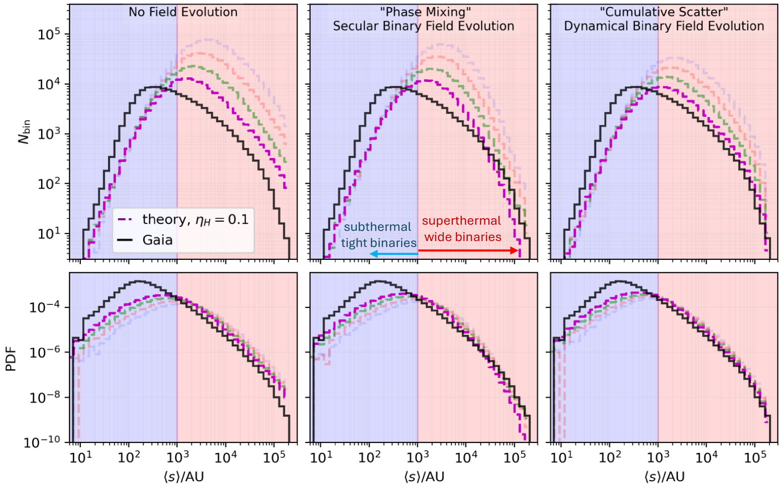
Figure 2:

Figure 3: The predicted number, $N_{\rm bin}$ (top), of 3BB’s within $200\rm pc$ of the Sun and their probability density function, (bottom), as a function of $\langle s\rangle$, projected average binary separation (Equation 4). The Gaia binary separations within 200 pc of the Sun are (black curve) taken from K. El-Badry et al. (2021) (with their ${<}0.1$ binary chance-alignment criterion). The left panel is the final distribution when applying “phase mixing” (PM, C.1) while the right panel uses the “cumulative scatter” prescription (CS, C.2). The CS prescription represents the most physically accurate model—it is highly improbable that a wide binary can secularly evolve in isolation over the course of the MW’s entire history. The overall shape of the separation distribution closely matches the observed distribution when $\langle s\rangle>10^{3}\rm AU$. The total number (i.e., from summing over $N_{\rm bin}$) of 3BBs is the number reported in Figure 1.

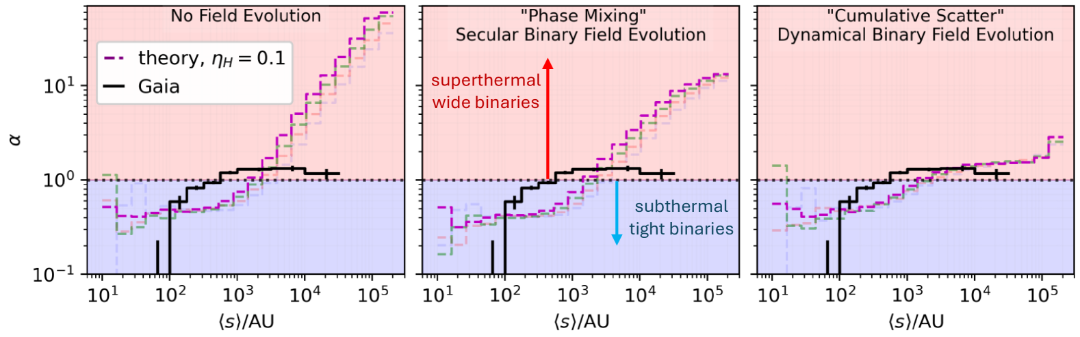
Figure 4:

Figure 5: The eccentricity parameter $\alpha\equiv\mathrm{d}\ln f/\mathrm{d}\ln\epsilon$ (Equation 5), as a function of the projected average binary separation, $\langle s\rangle$. Note that $\alpha=1$ corresponds to the thermal distribution, while $\alpha>1$ and $\alpha<1$ represent superthermal and subthermal distributions, respectively. The solid black line is the set of $\alpha$ values found by H.-C. Hwang et al. (2022b). In the left panel the colored dashed lines are the “phase-mixed” distributions (§ C.1.2). The right panel features the final eccentricity distributions following the “cumulative scatter” prescription (§ C.2). Phase mixing imparts only a slight “thermalization,” with the resultant wide binary distributions far more eccentric than what is observed. Rather, by considering dynamical encounters in the field, cumulative scattering imparts a dramatic thermalization, resulting in eccentricities in greater observational agreement with H.-C. Hwang et al. (2022b). Despite the simplicity of our toy model and the uncertainties surrounding Gaia-incompleteness, there is good qualitative agreement: wide binaries tend superthermal while tight binaries tend subthermal.

3 Mock Three-body Binary Population versus Gaia Wide Binaries

The entirety of our results stem from evaluating and interpreting the G3R (§ D, Equation D1), following the application of field evolution post-processing (§ C), and comparing to Gaia observations of binaries as compiled by K. El-Badry et al. (2021) and H.-C. Hwang et al. (2022b). Despite the several idealizations necessary to implement our semi-analytic model (e.g., equal-mass stars, universal Plummer clusters, circular and unchanging cluster orbits in the MW, etc.), our results share remarkable agreement with Gaia’s wide binary population in SMA and eccentricity distributions, and the total number within the solar neighborhood.

Figure 1 displays the total number of solar neighborhood 3BBs we predict across all our models, alongside the wide binary ($\langle s\rangle>10^{3}\rm AU$) tally. The “tidal isolation” parameter, $\eta_{H}$ (§ A.1), is a nuisance parameter quantifying how isolated a three-body encounter is from tidal perturbations applied by its host cluster. Smaller $\eta_{H}$ demands increasingly isolated three-body encounters, with $\eta_{H}=\{0.22,0.1\}$ excluding 3BBF if the maximum tidal acceleration applied to the three bodies by the cluster during the encounter is ${>}\{1\%,0.1\%\}$ of the three bodies’ maximum initial relative acceleration (see §A.1).

Though we may increase certainty in the physical “isolation” of a 3BBF event by shrinking $\eta_{\rm H}$, what constitutes “isolated enough” is unconstrained in the $N$-body literature. A slew of $\eta_{H}$ models are generated to show the effect of asserting ever more conservative tidal isolation during 3BBF. A clear trend presents itself in Figure 3: smaller $\eta_{H}$ dramatically constrains the 3BB creation probability, especially for the widest binaries. This is a direct result of the 3BBF rate scaling as $\eta_{\rm H}^{3}$ (§ A.1). Depending on $\eta_{H}$, the number of 3BBs our model predicts to currently be within $200\,\rm{pc}$ ($1\,\rm{kpc}$) of the Sun varies from ${\sim}10^{5}$–$10^{6}$ (${\sim}10^{6}$–$10^{7}$).

The choice of field evolution prescription heavily impacts the number and orbital element distributions of field binaries, with CS applying the most significant perturbations to individual binaries and the binary population as a whole. That said, both, the PM and CS binary field evolution prescriptions help bring the initially highly superthermal 3BB eccentricities in line with the more modestly superthermal observations. This is consistent with the conclusions of C. Hamilton (2022); C. Hamilton & S. Modak (2024), who postulated that the physical mechanism(s) responsible for creating the observed Gaia wide binaries would need to have a dramatic superthermal bias because of the thermalizing effect of stellar encounters and the Galactic tide after binary formation.

These 3BBs are the rare few that make a clean getaway from their natal cluster after formation. From Figure 1, the expected number of 3BBs escaping to the Galactic disk over a cluster’s life is

$$N_{\rm bin,cl}\approx 0.6\left(\frac{\eta_{H}}{0.1}\right)^{3}\left(\frac{M_{\rm cl0}}{10^{4}M_{\odot}}\right)^{0.9},$$ (3)

where $M_{\rm cl0}$ is the initial mass of the cluster, not the mass of the cluster at the point of 3BB emission. Despite the infrequency of 3BB formation, survival, and escape in individual low-mass clusters, our models suggest that the ubiquity of low-mass clusters makes them the largest contributors to a field 3BB population. The demographics of these binaries are discussed further in §§ 3.1 and 3.2, where the former strongly indicates 3BBF readily reproduces the observable Gaia superthermal wide binary population, alongside a meaningful contribution to the population of tight binaries.

3.1 Semi-major Axis and Eccentricity Distributions

To further compare the modeled and Gaia-observed binary populations, we express their respective SMA ($a$) and eccentricity ($\epsilon$) distributions in Figures 3 and 5 in terms of the average projected separation (H.-C. Hwang et al., 2022b):

$$\langle s\rangle=\frac{\pi}{4}a\left(1-\frac{\epsilon^{2}}{2}\right).$$ (4)

Figure 3 provides the most visually compelling agreement, especially when we conservatively limit our maximum allowable 3BBF encounter volume to ${\sim}10\%$ of the local cluster Hill Radius ($\eta_{H}=0.1$). According to our model, the suppression in the wide binary population at higher $\langle s\rangle$ is directly attributable to binary dissolution by disk encounters (Equation C2). The 3BBF ${\sim}a^{2.5}$ proportionality for hard binaries, as expressed in D. C. Heggie (1975); J. Goodman & P. Hut (1993) and numerically reproduced in § A.2, correlates with the observed Gaia curve for separations ${<}10^{3}\,\rm{AU}$. However, there is substantial evidence that the tight‐binary regime is highly incomplete (K. El-Badry & H.-W. Rix, 2018), so this apparent agreement is likely coincidental, implying that 3BBF can only play a supporting role in directly populating tighter binaries.

The orbital perturbations by disk encounters on 3BBs is modeled with greater physical realism in the CS prescription. It does not merely consider the absolute destruction or conservation of binaries evolving under constant, isolated, secular evolution by the Galactic tides (as in PM), but enables stochastic binary evolution in SMA and eccentricity. A gentler fall-off in the separations of the wide 3BB population results, with most binaries with $a>10^{4}\rm AU$ born tighter, with $a$ between $10^{3}-10^{3.5}\rm AU$ (discussed further in § 3.2). These tighter binaries end up populating the widest subset of binaries through CS evolution, mitigating losses due to the rapid destruction of binaries with initial SMA $>10^{4}\rm AU$. The impact of CS on the eccentricity distribution is far stronger than that of PM.

Turning to binary eccentricities, Figure 5 draws a set of fits for the eccentricity parameter, $\alpha$, with our two different field evolution prescriptions (§ C) and overlaid by the Gaia values calculated in H.-C. Hwang et al. (2022b). The $\alpha$ parameter is a convenient means to quantify how the eccentricity distribution compares to the thermal distribution. By fitting the expression

$$f(\epsilon)=(\alpha+1)\epsilon^{\alpha},$$ (5)

the $\alpha$ distribution is subthermal (less eccentric than thermal) if $\alpha<1$, thermal when $\alpha=1$, and superthermal if $\alpha>1$. It should be immediately apparent that the predicted and observed $\alpha$ values are not an exact match (variances within order unity). However, they are in good qualitative agreement; echoing exactly the observational findings of H.-C. Hwang et al. (2022b), our models show that binaries with $\langle s\rangle<10^{3}\rm{AU}$ tend subthermal while binaries with $\langle s\rangle>10^{3}\rm{AU}$ tend superthermal. The subthermal behavior is expected for binaries that form near the peak of the two-dimensional SMA–eccentricity distribution (where $a\approx R_{1}$, the radius of the three-body interaction volume; see § A.2).

The degree to which wide binaries exhibit a superthermal distribution varies dramatically between the PM and CS field evolution prescriptions (left panel and right panels of Figure 5, respectively). Because the PM prescription only has a cursory thermalizing effect, the eccentricity distributions of the widest binaries remain unreasonably superthermal. To the contrary, CS produces an $\alpha$ distribution in closer agreement with observations for wide binaries. As $\eta_{H}$ shrinks, both field evolution methods produce more eccentric binaries, though this is effect is small relative to how dramatically binary SMA and formation rate are affected by $\eta_{H}$.

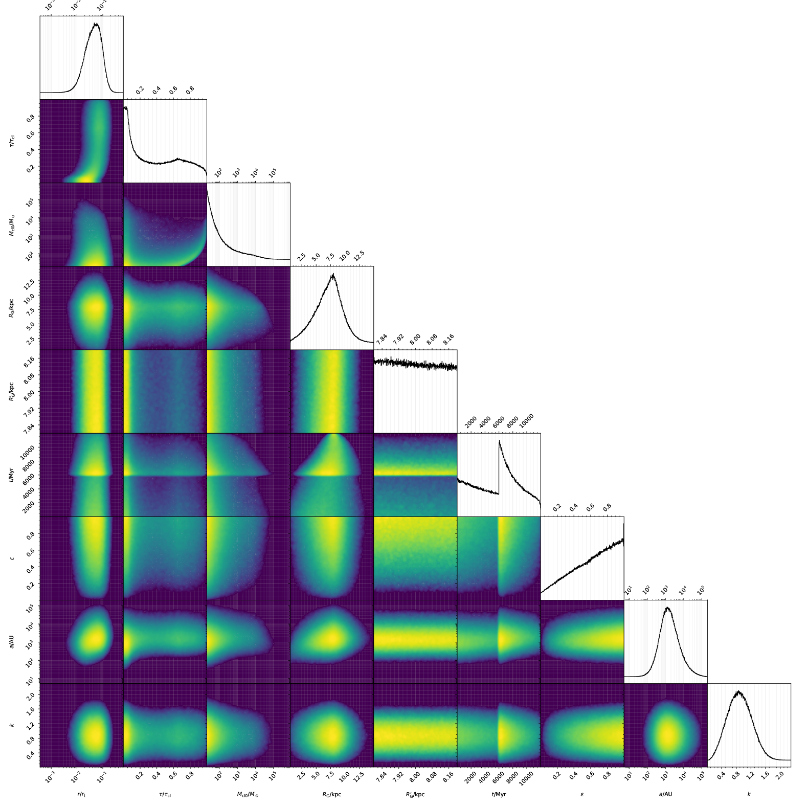
Figure 6: Grid of the resultant 9D, Galactic 3BBF Rate (G3R, Equation D1) distribution, as obtained by Monte Carlo integration with emcee (D. Foreman-Mackey et al., 2013), and projected as a set of 2D probability density functions for each dimensional combination. See Table 1 for a description of the independent variables. The sharp discontinuity in the $t$ dimension begins at the onset of star formation in the MW thin disk. This model was generated by fixing the maximum encounter volume to $10\%$ of the local cluster Hill Radius ($\eta_{\rm H}=0.1$, § A.1) and evolving field binaries with the “cumulative scatter” (CS) prescription (§ C.2). The grid was generated using the Python corner module (D. Foreman-Mackey, 2016).

Figure 7: These five subfigures are SMA-focused, “1.5-dimensional” versions of the contour plots in Figure 6, where color (the extra “0.5th” dimension) distinguishes between different logarithmically-spaced bins ($i$) in SMA of width $\Delta a_{i}$. The bottom panel of each subfigure displays the cumulative density functions, $C(X,a_{i})$, of the integration variable $X$ specified on the panels’ horizontal axes, for each bin in SMA. The top panels of each subfigure display the corresponding probability density functions scaled by SMA bin width, $f(X)\Delta a_{\rm i}=\frac{\partial^{2}C(X,a_{\rm i})}{\partial X\partial a}\Delta a_{\rm i}$. This scaling enables a direct comparison of the relative contributions to the total G3R from each bin in SMA. The integration variables under examination are (a: $\{r/r_{\rm h}\}$) radial cluster location of 3BBF in terms of the natal cluster’s half-mass radius, (b: $\{\tilde{\tau}\}$) time between cluster formation and 3BBF as a fraction of the total cluster lifetime, (c: $\{M_{\rm cl}\}$) mass of the 3BB’s natal cluster at time $\tilde{\tau}$, (d: $\{R_{G}\}$) Galactocentric radius of natal cluster, (e: $\{t\}$) time the 3BB escapes its natal cluster, where $t=12\,\rm Gyrs$ is the present day. The widest binaries tend to be born later in time, both in $\tilde{\tau}$ and $t$, and further out, both in $r/r_{\rm h}$ and $R_{\rm G}$, than tight binaries. Across the entire parameter space, we predict that solar neighborhood 3BBs mostly formed in clusters with masses $M_{\rm cl}<10^{3}\,M_{\odot}$ (at $\tilde{\tau}$), with more than half born in $M_{\rm cl}<50M_{\odot}$ clusters.

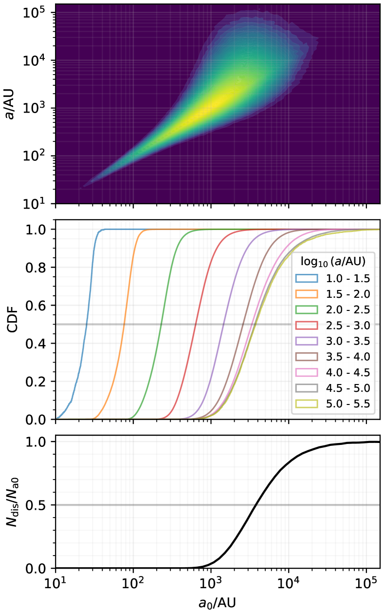
Figure 8: (i)

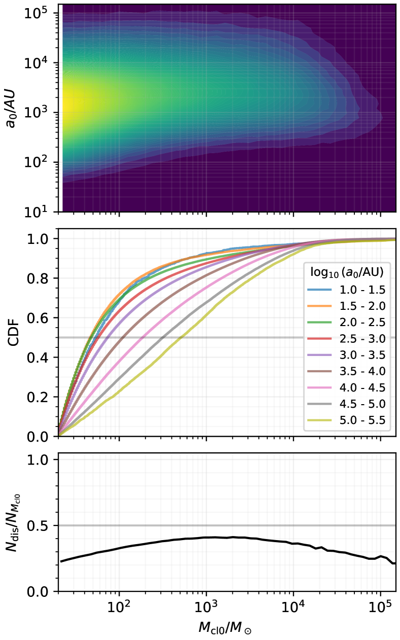
Figure 9: (ii)

Figure 10: Contour plots (top) and an accompanying set of cumulative distribution functions (middle) illustrating the relationship between (i) the initial binary SMA, $a_{0}$, and its final SMA, $a$, following CS field evolution, and (ii) $a_{0}$ and the initial mass of the binary’s natal cluster, $M_{\rm cl0}$. In column (ii), we include the samples of binaries eventually disrupted through CS. The bottom panels show the fraction of disrupted field binaries given (i) $a_{0}$ or (ii) $M_{\rm cl0}$. The tighter the initial binary, the less its SMA tends to change. Critically, we predict that wide field 3BBs in the solar neighborhood today with SMA $a>4000\,\rm{AU}$ are overwhelmingly born with $a_{0}<4000\,\rm{AU}$. Hence, the wider the initial binary, the more rapidly it is destroyed in the field. Separately, the least massive clusters tend to produce the highest numbers of initially tight binaries, with over $50\%$ of $a_{0}<10^{3}\,\rm{AU}$ binaries born in clusters with $M_{\rm cl0}<100\,M_{\odot}$. Low-mass clusters contribute much of the initially widest binaries, with more than $50\%$ of the initially widest binaries emitted from clusters with $M_{\rm cl0}<500\,M_{\odot}$, but these binaries are overwhelmingly disrupted by CS.

3.2 Formation Characteristics of Solar Neighborhood Three-body Binaries

Figure 6 broadly highlights the underlying distribution and dimensional covariance found by evaluating the G3R. There are a few intuitive takeaways here: (i) most field 3BBs are created early in a cluster’s life when it is densest, according to the united equations of evolution (UEE, § A.4), with the smallest binaries born almost exclusively in a cluster’s infancy, (ii) very few binaries have orbital radii which migrate more than $3\,\rm{kpc}$ through the disk, as expected from the N. Frankel et al. (2020) diffusion model (§ B.1), and (iii) there is a sharp preference for 3BBs to have escaped clusters born at the onset of star formation in the thin disk ($t=6$ Gyrs in N. Frankel et al. (2020)).

A more robust physical intuition may be found by examining “1.5-dimensional” versions of the contour plots relating binary SMA to cluster and MW history; they are displayed in Figure 7. Here, the dimensions (integration variables) of the G3R under scrutiny are (from left to right): $r/r_{h}$, the radial location within its host cluster where a 3BB is born, $\tilde{\tau}$, the fraction of the cluster’s lifespan elapsed when the 3BB forms and escapes, $M_{\rm cl}$, the mass of the cluster at the time of 3BBF and escape, $R_{G}$, the Galactocentric radius of the birth cluster’s circular orbit, and $t^{\prime}$, the age of the MW when the 3BB was born. Several interesting predictions are discernible here. First, nearly half of escaping 3BBs are born outside the host cluster’s Plummer core radius ($r\gtrsim 0.5r_{h}$), with wider binaries being born both further from the cluster’s center and later in the cluster’s life than tighter binaries. In fact, wide binaries tend to escape their birth cluster at a roughly uniform rate throughout the cluster’s life while ${>}50\%$ of the tightest 3BBs are born in the first ${\sim}10\%$ of the cluster’s life.

The overwhelming majority of 3BBs migrating to the solar neighborhood originate from low-mass clusters ($M_{\rm cl}<10^{3}\,M_{\odot}$) due to their dominance of the CIMF (Equation B4). Wide binaries exhibit a larger spread in natal cluster masses, while tight binary formation is heavily concentrated in clusters with $M_{\rm cl}<100\,M_{\odot}$. Additionally, our model predicts that the tightest, solar neighborhood 3BBs should be born uniformly through the MW disk from $R_{G}=1$–$8\,\rm{kpc}$ and early in MW star formation history, with $50\%$ born within the first $4\,\rm{Gyr}$ of the MW’s life (assuming a present MW age of $12\,\rm{Gyr}$). Wider binaries are born later in MW history and nearer to the solar neighborhood, an intuitive requirement due to the profound increase in a binary’s ionization cross section across orders of magnitude of binary SMA (§ C.1.1).

It has long been postulated that dissolving clusters should be a reliable environment for dynamical wide binary formation (M. F. Sterzik & R. H. Durisen, 1998; N. Moeckel & M. R. Bate, 2010; M. B. N. Kouwenhoven et al., 2010; N. Moeckel & C. J. Clarke, 2011). Yet, we do not find isolated 3BBF to be a significant mechanism for generating solar neighborhood binaries at cluster dissolution $(\tilde{\tau}\approx 1)$, in either initially low- or high-mass clusters. Admittedly, our idealized treatment of star clusters as single-component Plummer models evolving under the UEE (§ A.4) is unlikely to reliably model cluster dissolution. The conditions for isolated 3BBF may also be rare in a cluster with few (${\lesssim}50$) bodies, though there is evidence that binary formation in strong interactions involving more than three bodies at the center of a cluster could be a significant source of tight binaries (A. Tanikawa, 2013). Such binaries are formed during particularly strong spikes in the cluster’s central density. Even our idealized cluster model exhibits density spikes at dissolution, so a more nuanced investigation of binary formation in high-density regions may be required to better assess whether dissolution is an evolutionary phase with significant binary generation. That said, the models of M. B. N. Kouwenhoven et al. (2010) found that extremely wide binaries predominantly form at the point of cluster dissolution, with a median binary SMA ${>}5000\,\rm{AU}$. Under CS (§ C.2), very few of these binaries can survive in the field.

The left-hand panels of Figure 10 draw a relationship between the SMA before field evolution (pre-CS) and the final SMA of a 3BB population within the solar neighborhood today. As expected, the tighter the initial binary, the less CS shifts its SMA. A critical, population-level transition presents itself for the widest binaries: 3BBs with final SMAs ${>}4000\,\rm{AU}$ overwhelmingly escaped their natal clusters with initial SMAs ${<}4000\,\rm{AU}$. In other words, field evolution preferentially destroys the widest field 3BBs, replacing them with initially tighter binaries $({\sim}10^{3}$–$10^{3.5}\,\rm{AU})$.

If we were to turn off disruption during CS field evolution, the distribution of wide binary SMA would become egregiously skewed to very wide SMA. The dearth of such very-wide binaries in our models is simply due to disruption during field evolution, and not 3BBF disfavoring very-wide binary production. Thus, any prospective wide binary formation channel that matches the observed Gaia SMA distribution, while neglecting field evolution, cannot account for most of the Gaia wide binary population. This implies that cluster dissolution may not be the primary source of solar neighborhood wide binaries, since it preferentially forms very-wide binaries before even considering field evolution and disruption.

Finally, the relationship between initial binary SMA and the initial mass of the natal cluster is displayed in the right-hand panels of Figure 10. These distributions include the contribution of binaries which would ultimately be disrupted through CS, the left panel did not. Our models reinforce the general consensus that the field binary generation is dominated by low-mass clusters (N. Moeckel & C. J. Clarke, 2011).

4 Discussion & Summary

4.1 Comparison to Alternative Binary Formation Channels

Tight field binaries have historically been assumed to form primordially (R. R. King et al., 2012; M. R. Bate, 2014; R. J. Parker & M. R. Meyer, 2014), the remnants of which are the select few binaries that have avoided disruption. Recent state-of-the-art simulations from the Starforge collaboration do in fact find that many binaries form primordially in clusters (D. Guszejnov et al., 2023; J. P. Farias et al., 2024), with a primordial binary fraction ${\sim}40\%$. The majority are bound to the cluster with very wide SMAs and are unlikely to survive the ensuing dynamics in such a dense stellar environment. However, 3BBF may help serve as a complementary formation channel for tight subthermal binaries, the overwhelming majority of which originate almost exclusively in the earliest, densest stage of cluster history within our models. While we do not assert 3BBF as a prominent method for tight binary generation, primordial binary formation need not be the only means.

Wide Gaia binary formation channels have been more elusive, primarily because the proposed formation channels may produce many wide thermal binaries—e.g., cluster dissolution (M. B. N. Kouwenhoven et al., 2010; N. Moeckel & M. R. Bate, 2010; J. Peñarrubia, 2021)—or a few superthermal binaries—e.g., disk fragmentation (J.-E. Lee et al., 2017; S. Xu et al., 2023)—but not both in the required quantities. As highlighted in § 3.2, the tendency for binary field evolution is to accelerate the widening of binaries towards disruption. This implies that any prospective wide binary formation channel matching the observed Gaia distribution before applying field evolution cannot be the dominant source of the Gaia wide binary population. Such is the case for binary formation by cluster dissolution, preferentially forming extremely wide binaries before considering field evolution.

With 3BBF, the preferred outcome is the formation of highly eccentric wide binaries. Accounting for the disruptive capacity in clusters and field perturbations, 3BBF can circumvent many of the formation challenges, implying that 3BBs may contribute a significant fraction of wide binaries observable today.

4.2 Limitations and Future Work

For a first foray into assembling a Galactic 3BBF rate, we opted for a simple, physically motivated astrophysical model. Yet, there are several practical developments that could increase the model’s physical realism and self-consistency.

While we have devoted much effort to modeling binary destruction in the birth cluster (§ A.5) and Galactic field (§§ C.1.1 and C.2), we do not consider the effect of in-cluster dynamical interactions not fully disrupting an escaping 3BB en route out of its natal cluster. As with field evolution, these dynamical interactions will typically widen binaries that are as low-mass and wide as the ones we consider, while further thermalizing their eccentricities (D. C. Heggie, 1975). However, our conclusions are unchanged because additional thermalization can only push the 3BB eccentricity distributions in Figure 5 towards the more thermal Gaia eccentricities identified by H.-C. Hwang et al. (2022b). Additionally, while we incorporate a simple giant molecular cloud disruption recipe (§ C.2), we do not consider the possibility of disruption from other MW substructures, like dark matter subhalos or other star clusters. Incorporating said structures alongside a time-dependent density profile of the MW would help improve the physical accuracy of our framework and increase the destruction rate of 3BBs in the Galactic field.

Our methodology also neglects tidal circularization and orbital decay from isolated binary stellar evolution (BSE), such as common envelope physics. BSE would be especially important modeling the large concentration of extremely eccentric binaries expected to be produced by 3BBF (J. Stegmann et al., 2024). Predicting the stellar metallically of binary members would also require an accurate treatment of BSE, which we leave for future work.

Combining the cluster evolution equations from M. Gieles et al. (2011) and an equal-mass Plummer model is a powerful and convenient way to rapidly characterize and evaluate cluster properties across mass scales purely analytically. However, a more refined prescription for the structure and evolution of star clusters with realistic initial mass functions and stellar populations could greatly improve the physical realism of our model. Notably, black holes (BHs) play critical roles in the evolution of star clusters (D. Merritt et al., 2004; A. D. Mackey et al., 2007, 2008; P. G. Breen & D. C. Heggie, 2013; M. Morscher et al., 2015; M. Peuten et al., 2016; S. Chatterjee et al., 2017; K. Kremer et al., 2019; N. C. Weatherford et al., 2020, 2021; M. Gieles et al., 2021; M. Gieles & O. Y. Gnedin, 2023; D. Roberts et al., 2025). Their high masses, low velocities, and high local density after segregating to the cluster center make BHs the primary catalyst for assembling compact object 3BBs (e.g., N. Ivanova et al., 2005; M. Morscher et al., 2015; N. C. Weatherford et al., 2023)—and possibly for wider 3BBF more generally.

Modeling 3BBF in multi-mass clusters will require a semi-analytic treatment of unequal mass 3BBF. Exploring unequal-mass 3BBF for the first time, D. Atallah et al. (2024) determined that the pairing probabilities between unequal-mass bodies in a positive energy encounter generally favor the pairing of the two least massive bodies. This revised the prior notion that the two most massive bodies are the most likely to bind (e.g., M. Morscher et al., 2015), which is the case for three-body encounters with negative total energy, such as binary–single interactions (N. C. Stone & N. W. C. Leigh, 2019; Y. B. Ginat & H. B. Perets, 2021; B. Kol, 2021). Unequal-mass 3BBF also features subtle changes to the overall SMA and eccentricity distributions of 3BBs. Yet, the critical characteristics imparted by 3BBF, that (i) wide binaries tend to be superthermal and (ii) binaries with an SMA smaller than the radius of the interaction volume tend to be described by a thermal distribution, is not changed.

The degree to which these distributions diverge from equal-mass 3BBF is small for mass ratio variance within a factor of ${\sim}2$, so a significant modification to the overall demographic of Gaia binaries is unexpected. Hard binaries pairing a compact object with a star will be most affected by a proper unequal-mass treatment of 3BBF, as these systems tend to exhibit mass ratios far from unity. Unfortunately, the parameter space encompassing unequal-mass 3BBF is simultaneously immense and subtle. A semi-analytic fit appropriate for our G3R framework, or any other population-wide study, requires a dedicated investigation. Full $N$-body simulations will be important to mitigate uncertainties in employing the current semi-analytic model with low-mass clusters; in future work, we plan to conduct such simulations.

Our models are likely insufficient at characterizing binary formation during cluster dissolution, whether through 3BBF or more complicated scattering modes. M. B. N. Kouwenhoven et al. (2010) estimated a wide binary fraction present at cluster dissolution of $10\%$ to $20\%$. This corresponds to one to two wide binaries formed per cluster at dissolution, though N. Moeckel & C. J. Clarke (2011) found integrating their models forward in time by a factor of two diminished the binary survival rate by an order of magnitude. The overwhelming majority of these binaries would likely be destroyed in the field (with typical initial SMA $>5000\,\rm{AU}$), but the surviving few would boost the overall wide binary formation rate and enhance the relative contribution from short-lived low-mass clusters.

4.3 Summary

We have developed a semi-analytic Galactic three-body binary formation rate (G3R) and demonstrate that three-body binary formation (3BBF) efficiently produces highly eccentric wide binaries. Our model predicts that binaries with SMA ${<}10^{3}\rm AU$ exhibit subthermal eccentricities whereas binaries with SMA ${>}10^{3}\rm\,AU$ are superthermal. Without fine-tuning, this framework closely matches the observed SMA distribution of Gaia’s wide binaries (K. El-Badry et al., 2021) and qualitatively matches the eccentricity distributions of H.-C. Hwang et al. (2022b) when applying cumulative scatter binary field evolution constructed by C. Hamilton & S. Modak (2024). The predicted number of wide binaries in the solar neighborhood matches or exceeds that observed by Gaia, though we have not accounted for observational incompleteness or selection effects. However, these systematics primarily affect Gaia’s ability to observe binaries with separations $<200\rm AU$. Thus, 3BBF may be an essential formation channel for the widest field binaries.

Future investigations incorporating unequal-mass 3BBF, binary stellar evolution, unequal-mass clusters, more advanced cluster evolution, and improved Milky Way disk evolution models will greatly enhance the accuracy and realism of our framework, as will accounting for Gaia selection effects. If originating heavily from 3BBF, Gaia’s wide binaries are artifacts of the internal dynamics in our Galaxy’s dense stellar environments—especially those that may have dissolved by the present—and of the Galaxy’s evolutionary history. It immediately follows that Gaia wide binaries may be powerful probes of dissolved star clusters and of Galactic archaeology more broadly.

Appendix A Modeling Three-body Binary Formation in Star Clusters

A.1 The 3BBF Rate

From D. Atallah et al. (2024), the volumetric rate of encounters between three unbound bodies (3UBs) for a field of equal masses $m$ with a Maxwellian velocity distribution is

$$\tilde{\Gamma}_{3B}=\frac{d\Gamma_{3B}}{d\text{\makebox[0.0pt][l]{\ooalign{\hfil\hphantom{$V$}\hfil\cr\kern 0.80002pt--\hfil\cr}}}V}=\frac{2^{5/2}\pi^{3/2}}{3}n^{3}R_{1}^{5}\sigma,$$ (A1)

where $n$ is the local number density, $\text{\makebox[0.0pt][l]{\ooalign{\hfil\hphantom{$V$}\hfil\cr\kern 0.80002pt--\hfil\cr}}}V$ denotes volume, $\sigma$ is the local velocity dispersion, and $R_{1}$ is the radius of the largest spherical volume (henceforth the “interaction volume”) containing all three bodies during the encounter if those bodies were to follow straight-line trajectories.

The 3BBF rate is simply the 3UB encounter rate multiplied by the numerically determined probability of binary formation, $P_{F}$, in 3UB encounters with the given $n$, $R_{1}$, and $\sigma$. D. Atallah et al. (2024) calculated this semi-analytic 3BBF rate with similar initial scattering conditions to S. J. Aarseth & D. C. Heggie (1976a), setting $R_{2}=15R_{1}$. Here, $R_{2}$ is the offset distance between the slowest moving body and the interaction volume; the other two bodies are initiated further from $R_{1}$, at distances proportional to their randomly drawn initial velocity (assuming a Maxwellian velocity distribution with dispersion $\sigma$). In a dense cluster environment, however, if $R_{1}\sim r_{\rm sep}$, the average local interparticle distance, then it does not make sense for bodies to travel a distance $R_{2}=15R_{1}$; the individual bodies would likely have a strong encounter en route to the 3UB interaction, breaking the approximation of an isolated encounter. The equal-mass 3BBF scattering probability of D. Atallah et al. (2024) thus needs to be refined by reducing $R_{2}/R_{1}$ from $15$ to $3$. The resulting numerically determined 3BBF probability is

$$P_{F} =c_{0}\left(\frac{2b_{90}}{R_{1}}\right)^{2}=c_{0}\left(\frac{2Gm}{3\sigma^{2}R_{1}}\right)^{2},\ c_{0}=3.82,$$ (A2)

where $b_{\rm 90}=Gm/(3\sigma^{2})$ is the impact parameter in a gravitational two-body encounter that deflects the bodies by $90^{\circ}$ from their original trajectory. The same scattering and fitting method from D. Atallah et al. (2024) is used, limiting the domain to values of $R_{1}/(2b_{90})>10$ (see § 3.1 and Figure 4 in D. Atallah et al. (2024) for more information).

Using our equal-mass formation probability, the resulting volumetric formation rate is

$$\tilde{\Gamma}_{F,0}=P_{F}\tilde{\Gamma}_{3B} =c_{0}\frac{2^{9/2}\pi^{3/2}}{3^{3}}\frac{G^{2}m^{2}}{\sigma^{3}}n^{3}R_{1}^{3}$$ (A3)

$$=c_{0}\frac{2^{5/2}\pi^{3/2}}{3^{2}}\frac{G^{2}m^{2}}{\sigma^{3}}n^{2}k^{3}.$$

For convenience, $R_{1}$ is rewritten in terms of the average interparticle separation, $r_{\rm sep}=\left(\frac{3}{4\pi n}\right)^{1/3}$, becoming $R_{1}=kr_{\rm sep}$. The $G^{2}m^{2}n^{2}\sigma^{-3}$ scaling above is notably shallower than the classic $G^{5}m^{5}n^{3}\sigma^{-9}$ scaling found in detailed balance calculations (D. C. Heggie, 1975; J. Goodman & P. Hut, 1993) and recovered recently in our modern approaches (Y. B. Ginat & H. B. Perets, 2024; D. Atallah et al., 2024), which applies to the formation of hard binaries. Prior estimates fixate on hard 3BBF, whereas we enable both locally hard and soft 3BBF. By relaxing the limit on binding energy and, instead, enforcing a geometric limit based on particle separations, we recover a formation rate scaling far more enabling of 3BBF, albeit with arbitrarily small binding energies. In the limit of hard binary formation, the combination of Equations (A3) & (A7, see § A.2) yields the classic scaling.

The validity of the above equations are contingent upon $n\text{\makebox[0.0pt][l]{\ooalign{\hfil\hphantom{$V$}\hfil\cr\kern 0.80002pt--\hfil\cr}}}V\ll 1$. To generalize Equation (A1), and so allow the consideration of encounters with $n\text{\makebox[0.0pt][l]{\ooalign{\hfil\hphantom{$V$}\hfil\cr\kern 0.80002pt--\hfil\cr}}}V\simeq 1$, the expression

$$P_{\rm iso}d\lambda=e^{-\lambda}d\lambda,\ \lambda=n\text{\makebox[0.0pt][l]{\ooalign{\hfil\hphantom{$V$}\hfil\cr\kern 0.80002pt--\hfil\cr}}}V$$ (A4)

must be applied; $P_{\rm iso}$ is the distribution of isolated encounters (e.g., no other bodies present within $R_{1}$) under the assumption that the rate of encounters may be modeled as a Poisson process. Thus,

$$P_{\rm iso}d\lambda=3k^{2}e^{-k^{3}}dk$$ (A5)

where $k$ is the radius of the interaction volume in units of $r_{\rm sep}$.

It is straightforward to integrate over all $k$, but, realistically, tidal forces from the cluster will tear apart an encounter before it occurs if $k$ is large enough. To account for this, a transformation can be applied to values of $k$ appearing in Equation (A3), limiting the maximum possible interaction volume self-consistently. A convenient choice for the maximum value of $k$ is some fraction, $\eta_{\rm H}$, of the Hill Radius, $R_{H}\approx R_{1}\left(\langle m\rangle/M_{\rm cl}\right)^{1/3}$. In terms of $r_{\rm sep}$, the fraction of local Hill Radius in a Plummer cluster is $k_{H}=\eta_{H}(1+(r/b)^{2})^{-1/3}$, where $\eta_{H}$ is arbitrarily selected to be $\leq 1$; we explore the effects of conservatively limiting $\eta_{H}$ in our results (§ 3). The transformation applied is thus: $k\rightarrow k_{1}=\min(k,k_{H})$. Specified to the case of encounters within a single field, and including the Hill Radius limit, Equation (A3) becomes

$$\tilde{\Gamma}_{F} =P_{\rm iso}\tilde{\Gamma}_{F,0}=c_{0}\frac{2^{5/2}\pi^{3/2}}{3}\frac{G^{2}m^{2}n^{2}}{\sigma^{3}}k_{1}^{3}\,k^{2}e^{-k^{3}}.$$ (A6)

The above expression represents the net 3BBF rate across all possible $\{a,\epsilon\}$. In the next section, a 2D distribution function is assembled, allowing the 3BBF rate to be modeled as a function of $\{a,\epsilon\}$.

A.2 The SMA/Eccentricity Distribution

Figure 11: Eccentricity ($\epsilon$) and semi-major axis ($a$) distributions for 3BBF from the scattering experiments described in § A.1. Note we normalize $a$ by $R_{1}$, the radius of the interaction volume—the largest spherical volume containing all three bodies during the encounter if those bodies were to follow straight-line trajectories. The solid lines are the raw results of the scattering experiments while the dashed lines show the distributions as approximated by Equation (A7). Top: Eccentricity distribution for several $x=a/R_{1}$ bins. As found by Y. B. Ginat & H. B. Perets (2024) and D. Atallah et al. (2024), binaries with $a>R_{1}$ have $\epsilon$ distributions that become increasingly superthermal with increasing $a$, but are thermal when $a<R_{1}$; the $\epsilon$ distribution is actually subthermal for $x\in[10^{-0.75},10^{0.0}]$, but this is not to resolved above. Bottom: Normalized semi-major axis distribution. As predicted by D. C. Heggie (1975); J. Goodman & P. Hut (1993), $f(x)\propto x^{5/2}$ when $a\ll R_{1}$, though the latter quoted the distribution cumulatively as $C(x)\propto x^{7/2}$.

Prior to Y. B. Ginat & H. B. Perets (2024); D. Atallah et al. (2024), the joint SMA ($a$) and eccentricity ($\epsilon$) distribution of binaries formed exclusively through 3BBF were not known (S. J. Aarseth & D. C. Heggie, 1976b; J. Goodman & P. Hut, 1993; N. Ivanova et al., 2005). Y. B. Ginat & H. B. Perets (2024); D. Atallah et al. (2024) found that 3BBF features a constant, thermal distribution ($f_{F}(\epsilon)=2\epsilon$; see J. H. Jeans 1919) for binaries with an SMA $a<R_{1}$ and an increasingly superthermal distribution for all SMA in the regime $a>R_{1}$. There is a slight subthermal region that peaks between $10^{-0.75}$ and $1$. This subthermal region plays an outsized role in the eccentricity of tight binaries because the formation rate of binaries with $a<R_{1}$ peaks when $a\approx R_{1}$. Remarkably, the 2D $(\epsilon,a/R_{1})$ distribution exhibits (near-) scale-free behavior for regions of the parameter space corresponding to $\chi_{1}=R_{1}/(2b_{90})\gtrsim 10$. Thus, independent of the 3BBF probability, $P_{F}(\chi_{1}>10)$, the 2D probability density function $f(\epsilon,a/R_{1})\,d\epsilon\,da/R_{1}$ may be semi-analytically approximated with ease.

Employing the PySR symbolic-regression tool (M. Cranmer, 2023) and feeding it ${\sim}10^{9}$ $\{\epsilon,a/R_{1}\}$ samples from the new set of 3UB scatterings with $R_{2}=3R_{1}$ (generated to calculate Equation (A2)), the 2D PDF between $a$ and $\epsilon$ in the equal-mass, equal-velocity distribution limit may be approximated as

$$f_{F}(\epsilon,x)\,d\epsilon\,dx =\frac{1.98965\,\epsilon^{x}\,d\epsilon\,dx}{\epsilon^{3-2x}+\frac{0.088857}{\epsilon\,x^{2.5}}+\frac{1.25678}{x}+x^{\epsilon}}$$ (A7)

$$x=a/R_{1},\ dx=da/R_{1},R_{1}=k_{1}r_{\rm sep},$$

where we have employed the Hill Radius correction in $k_{1}$ (§ A.1) and is normalized over the domain $\{{\epsilon\in[0,1]},\ {x\in(0,\infty)}\}$. The $a$ and $\epsilon$ distributions from our 3UB simulation data and semi-analytic approximation are displayed in Figure 11. Like J. Goodman & P. Hut (1993), we find that the hardest/closest binaries ($a\ll R_{1}$) exhibit a 3BBF SMA distribution $\propto a^{5/2}$. This SMA scaling just so happens to be identical to the observed close-binaries in the Gaia binary curve (§ 3.1). Updating the 3BBF formation rate by incorporating a dependence on $(\epsilon,a)$ and $k$, it may be written

$$\frac{d^{3}\tilde{\Gamma}}{dk\,d\epsilon\,dx}=\tilde{\Gamma}_{F}f_{F}(\epsilon,x).$$ (A8)

A.3 3BBF in a Plummer Cluster

Our focus is to estimate the rate of 3BBF in stellar clusters. As we introduce nine integration variables, the calculation will quickly become intractable unless we employ a simple analytic cluster model, such as a Plummer model, to estimate local cluster properties. For future reference, some useful Plummer expressions include

$$\rho=\frac{3M_{\rm cl}}{4\pi b^{3}\left(1+(r/b)^{2}\right)^{5/2}},\ \Phi=-\frac{GM_{\rm cl}}{b\left(1+(r/b)^{2}\right)^{1/2}},\ \sigma^{2}=-\frac{\Phi}{6},\ v_{\rm esc}=\sqrt{12}\sigma,\ \ b=(2^{2/3}-1)^{1/2}r_{\rm h}$$ (A9)

where $\rho=\langle m\rangle n$, $n$, $\Phi$, $\sigma$, $M_{\rm cl}$, $\langle m\rangle$, $b$, and $r$ are the local mass density, number density, potential energy, one-dimensional velocity dispersion, total cluster mass, average mass, Plummer scale-length (or kernel), and radial distance from the center of the Plummer cluster, respectively.

Equation (A8) may be written in terms of the Plummer relations, becoming

$$\frac{d^{3}\tilde{\Gamma}}{dk\,d\epsilon\,dx}=\frac{d^{4}\Gamma}{d\text{\makebox[0.0pt][l]{\ooalign{\hfil\hphantom{$V$}\hfil\cr\kern 0.80002pt--\hfil\cr}}}Vdk\,d\epsilon\,dx}=\frac{d^{4}\Gamma}{4\pi r^{2}dr\,dk\,d\epsilon\,da/R_{1}},$$ (A10)

$$\frac{d^{4}\Gamma}{drdkd\epsilon da}=36c_{0}\sqrt{\frac{3G\langle m\rangle}{\pi b^{7}}}\left(\frac{M_{\rm cl}}{\langle m\rangle}\right)^{5/6}k_{1}^{2}k^{2}e^{-k^{3}}\frac{(r/b)^{2}}{(1+(r/b)^{2})^{61/12}}f_{F}\left(\epsilon,\frac{a}{k_{1}r_{\rm sep}(r)}\right).$$

We have written the 3BBF rate in terms of the radial displacement in the Plummer cluster, $r$, and SMA, $a$, instead of $\text{\makebox[0.0pt][l]{\ooalign{\hfil\hphantom{$V$}\hfil\cr\kern 0.80002pt--\hfil\cr}}}V$ and $x=a/R_{1}$ for integration convenience. In the final portion of the calculation (§ D), the substitution $r\rightarrow r_{t}\tilde{r}$ is applied to limit the integration boundary within the tidal radius of the Plummer cluster; $\tilde{r}$ is the radial displacement normalized by the tidal radius of the cluster. Equation (A10) is the “local creation rate” and we will not consider any other means to form binaries, whether through 3BBF outside of a Plummer cluster or other binary formation mechanisms. The “creation rate” is now written

$$\frac{d^{4}\Gamma}{drdkd\epsilon da}\equiv\mathcal{C}(M_{\rm cl},b,r,k,\epsilon,a)$$ (A11)

for æsthetic compactness. Subsequent sections will assemble probability distributions describing the evolution of individual clusters and the Milky Way or binary disruption in the cluster or the field .

A.4 Cluster Evolution

Emphasizing practicality over absolute accuracy, we adopt the M. Gieles et al. (2011, Appendix C) Unified Equations of Evolution (UEE) cluster model for its simplicity and natural compatibility with the entirety of the nine-dimensional distribution function under assembly. While these models are not intended to provide exact predictions, they are a convenient approximation to apply across a wide range of cluster masses, $M_{\rm cl}$, and Galactocentric orbital radii, $R_{G}$. Comparing the analytic timescales of Appendix A, UEE in Appendix C, and Table 2 (all found in M. Gieles et al. (2011)), the UEE become

$$M_{\rm cl}(M_{\rm cl0},\tilde{\tau})=M_{\rm cl0}\left(1-\tilde{\tau}\right)^{4/3},\ M_{\rm cl0}=\langle m\rangle N_{\rm cl0},\ \tilde{\tau}=\tau/\tau_{\rm cl},$$ (A12)

$$\tau_{\rm cl}(N_{\rm cl0},R_{G})=0.13N_{\rm cl0}^{3/4}\frac{R_{G}}{V_{G}},$$

$$r_{\rm h}(M_{\rm cl},R_{G})=0.66\zeta^{2/3}r_{t}(M_{\rm cl},R_{G})\,\frac{\ln\left[\Lambda(N_{\rm cl})\right]^{2/3}}{N_{\rm cl}^{1/6}}\left(1-\left(1-\tilde{\tau}\right)^{11/3}\right)^{2/3},$$

$$r_{t}(M_{\rm cl},R_{G})=\sqrt[3]{\frac{GM_{\rm cl}(\tilde{\tau})}{2}\left(\frac{R_{G}}{V_{G}}\right)^{2}},$$

where $M_{\rm cl0}$ is the initial cluster mass, $\langle m\rangle$ is the average cluster mass, $\tau$ is the amount of time elapsed since the cluster expelled most of its gas following the onset of star formation, $\tau_{\rm cl}$ is the predicted lifetime of a cluster, $M_{\rm cl}$ and $N_{\rm cl}$ are the cluster mass and cluster particle number at time $\tilde{\tau}$, $R_{G}$ and $V_{G}\equiv V_{G}(R_{G})$ are the Galactocentric radius and Milky Way circular velocity at $R_{G}$ (see § B.1), $\Lambda(N_{cl})$ is the argument of the Coulomb Logarithm, $r_{t}(M_{\rm cl},R_{G})$ is the tidal radius of the cluster, and $\zeta=0.15$ is the cluster heating constant. Additionally, our expression for $r_{h}$ is fixed to $r_{h}(\tilde{\tau}=0.05)$ for all times $\tilde{\tau}<0.05$ due to the unrealistically high initial cluster densities predicted by the UEE.

The argument of the Coulomb Logarithm, $\Lambda(N)$, is an object of frequent debate, often approximated for small subsets of the $N$-Body parameter space. Traditionally, $\Lambda$ is given the form $\Lambda=\frac{b_{\rm max}}{b_{\rm min}}$, where $b_{\rm max}$ and $b_{\rm min}$ are the maximum and minimum impact parameters considered in scattering encounters between individual bodies in an $N$-Body system (J. Binney & S. Tremaine, 2008). M. Giersz & D. C. Heggie (1996) prescribes a value of $\Lambda\approx 0.02N_{\rm cl}$ for $N_{\rm cl}\sim 10^{5}$, though they find that the argument should be much larger for smaller values of $N$, becoming $\Lambda\approx 0.1N_{\rm cl}$ if $N_{\rm cl}\sim 250$. A convenient analytic expression which qualitatively and quantitatively bridges the extremes of the parameter space falls out of setting $b_{\rm max}=r_{\rm sep}(r_{h})$ and $b_{\rm min}=b_{90}(r_{h})$; $r_{\rm sep}(r_{h})$ is the average inter-particle distance and $b_{\rm 90}(r_{h})=\frac{Gm}{3\sigma(r_{h})^{2}}$ is the $90$-degree deflection angle between equal masses living at the cluster half-mass radius in a single-component Plummer model. The resulting functional form is

$$\Lambda(N_{\rm cl})=\frac{N_{\rm cl}^{2/3}}{2}\left(1-2^{-2/3}\right)^{-1/3}\approx 0.7N_{\rm cl}^{2/3},$$ (A13)

which we have adopted across all cluster masses.

Figure 12 displays a host of cluster properties—born on circular orbits at $R_{G}=8\,\rm{kpc}$—as they evolve through their cluster lifetime, $\tilde{\tau}=\tau/\tau_{\rm cl}$. The cluster is dissolved when $\tilde{\tau}=1$. For example, a cluster born with $M_{\rm cl0}=10^{3.3}\,M_{\odot}$ will have a half-mass radius of $r_{h}\approx 1.5\,\rm{pc}$ after shedding half its initial mass through relaxation and Galactic tides. All the cluster properties are in qualitative agreement with the set of cluster $M_{\rm cl},r_{\rm h}$ observations compiled in M. R. Krumholz et al. (2019).

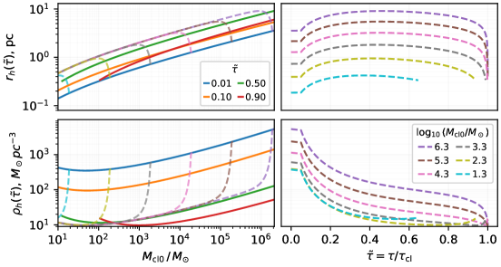
Figure 12: Assumed semi-analytic relations between cluster properties—initial mass $M_{\rm cl0}$, half-mass radius $r_{h}$, and density $\rho_{h}$ within the half-mass radius, and age $\tilde{\tau}$ normalized by cluster lifespan—according to our compilation of the UEE from M. Gieles et al. (2011)—Equations (A12). In the left column, the solid curves show the $r_{h}$–$M_{\rm cl0}$ relation (top) and $\rho_{h}$–$M_{\rm cl0}$ relation (bottom) at several cluster ages indicated by color. The time evolution of $r_{h}$, $\rho_{h}$ and $M_{\rm cl}$ for several specific choices of initial cluster mass $M_{\rm cl0}$ are indicated by the dashed curves in both the left and right columns. The early truncation of the dashed yellow and light blue curves prior to $\tilde{\tau}=1$ (cluster dissolution) reflect our choice to halt cluster evolution once there are fewer than 10 bodies, below which these semi-analytic approximations break down. All clusters shown are assumed to evolve on a circular orbit about the Milky Way center at an equivalent Galactocentric radius to the sun ($R_{G}=8\,\rm{kpc}$).

A.5 Escape & Disruption in a Stellar Cluster

Two criteria are required for a 3BB to escape a cluster: (i) the center-of-mass (CoM) velocity of the new binary must exceed the local escape speed of the cluster and (ii) the binary must not undergo any strong (ionizing) encounters en route out of the cluster’s gravity well. By definition, wide binaries are very easy to disrupt and so this calculation should be done precisely as to not overestimate their survival rate.

Two key equations will be necessary for the calcuating the survival and escape probabilities along the approximately radial path the binary takes, the first being the standard Maxwellian velocity distribution

$$f_{M}(v,\sigma_{b})=\sqrt{\frac{2}{\pi}}\frac{v^{2}}{\sigma_{b}^{3}}e^{-v^{2}/(2\sigma_{b}^{2})},\ \sigma_{b}^{2}(\tilde{r})=\sigma^{2}(\tilde{r})+\frac{Gm}{18a}$$ (A14)

where $\sigma_{b}$ is the velocity dispersion of the new binary at $\tilde{r}$. Assuming 3BBF between equal masses, the mean-square velocity kick imparted to the new binary is $Gm/(6a)$. The second equation is the equal-mass ionization cross section (P. Hut & J. N. Bahcall, 1983)

$$\Sigma_{\rm ion}=\frac{20\pi}{3}\frac{Gm}{v_{\rm rel}^{2}}a$$ (A15)

where $v_{\rm rel}=\sqrt{v_{\rm b}^{2}+v^{2}}=\sqrt{12\sigma^{2}(\tilde{r})+v^{2}}$ is the relative velocity between the target binary and a single star. We only consider the fraction of 3BB’s formed with a CoM velocity greater than the local escape speed and make the simplifying assumption that their velocity is always equal to the local escape speed and on a radial trajectory. Larger velocities act to suppress the ionization rate, but the fraction of 3BBF’s with CoM velocities greater than $1.2v_{\rm esc}$ is vanishingly small, and so we choose to ignore this subtly in favor of accounting for the slowing of the binary as it exits the cluster.

Employing $\Sigma$ for a trivial “N-$\Sigma$-V” calculation, the ionization rate is

$$\Gamma_{\rm ion} =\left\langle n\,\Sigma\,v_{\rm rel}\right\rangle=\frac{20\pi}{3}nGma\left\langle\frac{1}{v_{\rm rel}}\right\rangle,$$ (A16)

$$\left\langle\frac{1}{v_{\rm rel}}\right\rangle= \int^{\infty}_{0}\frac{f_{M}(v,\sigma)}{\sqrt{12\sigma^{2}+v^{2}}}dv=\frac{\alpha_{0}}{\sigma},\ \ \alpha_{0}\approx 0.260434$$

and the expected number of ionizing encounters for an escaping binary becomes

$$\lambda_{\rm ion,out}(r,M_{\rm cl},b,a)=\int^{r_{t}}_{r}\Gamma_{\rm ion}(r)\frac{dr}{v_{b}}=\frac{5\sqrt{3}\,\alpha_{0}\,}{2}\frac{a}{b}\left[\frac{\pi}{2}-f_{\lambda}(r)\right],$$ (A17)

$$f_{\lambda}(r)=\frac{r/b}{1+(r/b)^{2}}+\tan^{-1}(r/b)$$

where $r$ is the birth location of the 3BB and where it begins its getaway. The fraction of 3BB’s paired with CoM velocity $v_{b}>v_{\rm esc}(\tilde{r})$ is

$$P_{\rm esc}(\tilde{r},M_{\rm cl},b,a)=2\sqrt{\frac{6}{\pi}}\frac{\sigma}{\sigma_{b}}e^{-6(\sigma/\sigma_{b})^{2}}+\rm{Erfc}\left(\sqrt{6}\frac{\sigma}{\sigma_{b}}\right),\ \ \sigma_{b}^{2}=\sigma^{2}+\frac{Gm}{18a}.$$ (A18)

Assuming a Poison process, the probability of a 3BB securing a clean escape with absolutely no ionizing encounters is

$$P_{\rm ion,out}(\tilde{r},M_{\rm cl},b,a)=e^{-\lambda_{\rm ion,out}}$$ (A19)

There are two escape trajectories to consider: (i) the binary travels on a radial path out of the cluster, Equation (A19), and (ii) the binary travels on a radial path inwards through the core of the cluster before continuing out of the cluster. Binaries taking an “inward” path have a survival probability equivalent to $P_{\rm ie,in}\approx P_{\rm ie,out}P_{\rm 0\rightarrow r}$. Here, $P_{\rm 0\rightarrow r}$ is the probability of no binary ionization after passing twice through the region spanning $0\rightarrow r$. Stated mathematically,

$$P_{\rm ion,in}=P_{\rm ion,out}e^{-\lambda_{\rm ion,in}},\ \ \lambda_{\rm ion,in}=5\sqrt{3}\,\alpha_{0}\frac{a}{b}f_{\lambda}(r)$$ (A20)

with the total probability of a clean escape

$$P_{\rm ie}\left(\tilde{r},M_{\rm cl},b,a\right) =P_{\rm esc}P_{\rm ion},\ \ P_{\rm ion}=\frac{e^{-\lambda_{\rm ion,out}}}{2}\left(1+e^{-\lambda_{\rm ion,in}}\right),$$ (A21)

where we take the average of the two possibilities.

Appendix B Star Formation History and Radial Diffusion in the Milky Way’s Disks

Up until § A.5, we only considered dynamics internal to toy Milky Way stellar clusters. To estimate the number and orbital element distributions of 3BB’s in the solar neighborhood, it is critical to model the relationship between the clusters hosting 3BBF, the MW disk, the cluster birth time, $t$, and Galactocentric radius, $R_{G}$, in the Milky Way thin and thick disks, and the journey (i.e., angular momentum diffusion) the few 3BB’s managing to escape their home clusters must take to reach a comparatively small spatial region within $\sim 200\,\rm{pc}$ of the Sun.

We may accomplish this by combining the thick disk model from T. Wagg et al. (2022) with the updated thin disk model of N. Frankel et al. (2020); T. Wagg et al. (2022) employed an older thin disk model. These models are a set of smooth semi-analytic distribution functions, tuned to reproduce the present day characteristics observed in the Milky Way. We highly recommend the reader carefully review their works for detailed information—only the set of distributions as implemented for our purposes are highlighted here.

The MW circular velocity curve is assumed to be constant across its total lifetime, $\tau_{\rm MW}=12\,\rm{Gyrs}$, and is taken exactly from the modeling scripts provided by A.-C. Eilers et al. (2019). All references to the circular velocity as a function of the Galactocentric radius, $R_{G}$, should be interpreted as their full functional form, $v_{c}(R_{G})$ (all stellar components + halo), as displayed in Figure 1 of A.-C. Eilers et al. (2019). Every orbiting body, whether stars or stellar clusters, are assumed to be on circular orbits. Escaping binary stars are the only objects we consider to be undergoing diffusion throughout the disk while clusters are evolved assuming fixed $R_{G}$. Finally, our toy galaxy is entirely composed of equal-mass, $0.5M_{\odot}$ stars, as we are only interested in evaluating the feasibility of forming local field 3BBs, not an attempted reproduction of the exact stellar and compact object sub-populations observed in Gaia.

B.1 Milky Way Disk Evolution

Restating our assumption that all stars are born in clusters, a star formation history model is, implicitly, a cluster formation history. The normalized set of equations describing the formation and dynamical evolution of bodies in the thick disk may be written

$$f_{ha}(R_{G})=\frac{R_{G}}{R_{d0}^{2}}e^{-R_{G}/R_{d0}},$$ (B1)

$$SFH_{\rm ha}(t)=\begin{cases}\frac{e^{-t/\tau_{SFR}}}{\tau_{SFR}\,\left(1-e^{-\tau_{ha}/\tau_{SFR}}\right)},&t<\tau_{ha}\\ 0,&t>\tau_{ha}\end{cases}$$

$$D_{\rm ha}(t^{\prime},R_{G},R_{G}^{\prime})=\sqrt{\frac{2\tau_{m}}{\pi\,t^{\prime}}}\exp\left[-\frac{\left(R_{G}^{\prime}-R_{G}+\frac{c_{1}^{2}\,t^{\prime}/\tau_{m}}{2R_{\rm d0}}\right)^{2}}{2c_{1}^{2}\,t^{\prime}/\tau_{m}}\right]{\rm Erfc}\left[\frac{c_{1}^{2}\,t^{\prime}/\tau_{m}-2R_{G}R_{d0}}{2\sqrt{2\,t^{\prime}/\tau_{m}}\,c_{1}R_{\rm d0}}\right]^{-1},$$

where $R_{d0}=2.3\,\rm kpc$ is the disk scale-length, $R_{G}$ is the Galactocentric distance of the cluster’s orbit and the starting point from which escaping 3BBs begin their disk migration, $t$ is the time separation between the MW’s birth (assumed to occur $\tau_{\rm MW}=12\,\rm Gyrs$ ago) and the cluster’s birth, $\tau$ is the time between cluster birth and formation of the binary, $t^{\prime}=\tau_{\rm MW}-\tau-t$ is the lookback time since a 3BB formed in a cluster, and $R_{G}^{\prime}$ is the location of the binary at $t^{\prime}$. Additionally, $\tau_{SFR}=6.8\,\rm Gyrs$ is the star formation timescale of the thick disk, $\tau_{ha}=6\,\rm Gyrs$ is the time when new cluster formation is “turned off” in the thick disk, $\tau_{m}=6\,\rm Gyrs$ is a timescale controlling the diffusion strength in the disk, and $c_{1}=2.48\,\rm{kpc}$ is the diffusion scale length. For simplicity, the latter two quantities and the form of the diffusion distribution, $D_{ha}$, are assumed identical to that of the thin disk models given by N. Frankel et al. (2020).

The equations describing the thin disk’s evolution are mostly identical to the above equations—namely $f_{\rm la}$ and $D_{\rm la}$—with the caveat that $R_{d0}\rightarrow 2.8\,\rm kpc$ and that $SFH_{\rm la}(t)$ features “inside out growth.” In other words, the star formation rate is higher at earlier times closer to the MW center, while “turning on” at later times and farther out from the Galactic center. Ported from N. Frankel et al. (2020) and normalized to a birth look-back time of $\tau_{la}=6\,\rm Gyrs$, the star formation history of the thin disk is

$$SFH_{\rm la}(t,R_{G})= \begin{cases}\frac{y\,e^{y(\tau_{\rm MW}-\tau_{la}-t)/\tau_{SFR}}}{\tau_{\rm SFR}\left(1-e^{-y\,\tau_{la}/\tau_{SFR}}\right)},&\tau_{ha}<t<\tau_{MW}\\ 0,&\rm{otherwise}\end{cases}$$ (B2)

$$y=1 -\frac{R_{G}}{12.6\,\rm kpc},$$

where $\tau_{la}=6\,\rm\,Gyr$ and $\tau_{SFR}=1\,\rm\,Gyr$. T. Wagg et al. (2022) constructed their Milky Way model assuming a total stellar mass $M_{d}=2.6\times 10^{10}M_{\odot}$ in each of the thick and thin disks and a bulge mass $M_{b}=0.9\times 10^{10}M_{\odot}$ (T. C. Licquia & J. A. Newman, 2015). To incorporate the stellar mass contribution from the bulge, we treat the bulge of the Milky Way as being built up from the combined stellar diffusion in the thick and thin disks, applying all the mass of the bulge to the older thick disk. The number of stars in each present-day disk are $N_{\rm ha}=\frac{M_{d}+M_{b}}{m}=7\times 10^{10}$ and $N_{\rm la}=\frac{M_{d}}{m}=5.2\times 10^{10}$, respectively. Combining the two disk distributions, our evolving MW disk model is

$$\mathcal{DHL}(t,R_{G},R_{G}^{\prime})=N_{\rm ha}f_{\rm ha}(R_{G})SFH_{\rm ha}(t)D_{\rm ha}(t^{\prime},R_{G},R_{G}^{\prime})+N_{\rm la}f_{\rm la}(R_{G})SFH_{\rm la}(t^{\prime},R_{G})D_{\rm la}(t^{\prime},R_{G},R_{G}^{\prime}).$$ (B3)

B.2 The Cluster Initial Mass Function

A cluster mass function (CMF) of the form $f(M_{\rm cl0})\propto M_{\rm cl0}^{-2}e^{-M_{\rm cl0}/M_{c}}$ is well-established observationally. The exponential (or Schechter) cutoff applies a smooth means to regulate the maximum allowable cluster mass in a galaxy (P. Schechter, 1976; B. G. Elmegreen, 2006; M. Gieles et al., 2006; S. F. Portegies Zwart et al., 2010; A. Just et al., 2023). When in a galaxy’s history and where in a galactic environment a CMF is established remains a field of active inquiry, but progress has been made in connecting observed star formation rates to the cluster masses which preceded star formation epochs (M. Gieles, 2009; L. C. Johnson et al., 2017; N. Choksi & J. M. D. Kruijssen, 2021). Based on the preceding literature, we can construct a cluster initial mass function (CIMF) compatible with our MW evolution model (§ B.1).

First, let’s assert the form of the CIMF distribution

$$f_{\rm CIMF}(M_{\rm cl0},t,R_{G})\propto M_{\rm cl0}^{-2}e^{-M_{\rm cl0}/M_{c}(t,R_{G})}$$ (B4)

where $M_{c}(t,R_{G})$ is the time- and Galactocentric radius-dependent cutoff of the Schechter function. Considering that L. C. Johnson et al. (2017) empirically found that $M_{c}$ may be related to the star formation rate surface density, $\Sigma_{\rm SFR}$, with the expression

$$\log_{10}\left(\frac{M_{c}}{M_{\odot}}\right)=1.07\log_{10}\left(\frac{\Sigma_{\rm SFR}}{M_{\odot}\rm{yr}^{-1}\rm{kpc}^{-2}}\right),$$ (B5)

we choose to extend the dimensionality of the equation by additionally asserting that $\Sigma_{\rm SFR}\equiv\Sigma_{\rm SFR}(t,R_{G})$. In our combined N. Frankel et al. (2020); T. Wagg et al. (2022) prescription, the Milky Way’s $\Sigma_{\rm SFR}$ is implicitly

$$\Sigma_{\rm SFR}(t,R_{G}) =\frac{M_{d}+M_{b}}{2\pi R_{G}}f_{\rm ha}(R_{G})SFH_{\rm ha}(t)+\frac{M_{d}}{2\pi R_{G}}f_{\rm la}(R_{G})SFH_{\rm la}(t,R_{G})$$ (B6)

which is related to $M_{c}(t,R_{G})$ using Equation (B5). The resulting normalization for Equation (B4) is

$$f_{\rm CIMF}^{\rm norm}(\tilde{M}_{\rm norm})=\frac{\tilde{M}_{\rm norm}}{e^{-\tilde{M}_{\rm norm}}+\tilde{M}_{\rm norm}(0.1485+E_{1}(\tilde{M}_{\rm norm}))},\ \ \tilde{M}_{\rm norm}=M_{\rm min}/M_{c}(t,R_{G})$$ (B7)

where $M_{\rm min}=20\,M_{\odot}$ is the smallest cluster mass we consider in the CIMF. Equation (B4) is normalized between $M_{\rm min}$ and $M_{c}(t,R_{G})$ since we consider $M_{c}$ to be the largest possible cluster mass in a star forming region (see also N. Choksi & J. M. D. Kruijssen, 2021).

Appendix C Field Evolution of Ejected Three-body Binaries

Binary evolution in the field is dependent on the internal stellar dynamics (e.g., tidal torquing & binary stellar evolution) and the extrinsic MW secular dynamics and non-secular stellar encounters (e.g., orbital perturbations and disruptions). Our scope is limited to the case of typical (low-mass) stellar binaries, with separations large enough that the internal stellar dynamics are negligible on long time-scales, and only broadly care about the orbital properties of field 3BBs. Thus, our modeling of binary field evolution is solely dedicated to the extrinsic dynamical effects in the MW disk en route to the solar neighborhood.

Two works form the foundation of our field evolution prescriptions: C. Hamilton (2022) and C. Hamilton & S. Modak (2024). C. Hamilton (2022) explored the MW secular dynamics and evolution of field binaries, a process named “phase mixing,” while C. Hamilton & S. Modak (2024) modeled the cumulative effect of many weak scattering encounters imparted to field binaries—“cumulative scatter” for short. It is not straightforward to consider both of these field evolution prescriptions simultaneously, so we treat these works as bifurcating paths, both of which we explore. Application of phase mixing (PM) is discussed in § C.1.2 and cumulative scatter (CS) in § C.2.

C.1 Binary Disruption and Phase Mixing

C.1.1 Wide Binary Disruption in the Disk

Binary disruption in the disk due to stellar encounters is not included a priori through phase mixing. Appending a disruption survival probability, $P_{\rm d,MW}$ (Equation C2), to our final equation (Equation D1) is an easy fix. The details of our $P_{\rm d,MW}$ derivation is discussed in § C.1.1. The resulting distribution in Equation (D1) returns the total number of binaries when integrated, but with initially unevolved binary samples. Their orbital elements remain identical to what was assigned at formation in the cluster; it is to this final distribution of surviving binaries we apply phase mixing, as described in § C.1.2.

The fraction of binaries which “diffuse” to a present-day Galactocentric orbit, $R_{G}^{\prime}$, will naturally be curtailed by strong scattering encounters in the disk. It is naturally preferable to consider an evolving disk model, accounting for the changing number and density of bodies in the disk with look-back time, $t^{\prime}$ (i.e., the time the binary is born and escapes the cluster). To avoid numerous intractable difficulties in the calculation, we instead adopt the conservative simplifying assumption of a constant disk density equal to the present-day density distribution.

A disk-survival model may be constructed by first writing the classic disruption rate (J. Binney & S. Tremaine, 2008)

$$\Gamma_{d}(R_{G})=\frac{22.7\,G\,a\ln(\Lambda_{d})}{\sigma_{\rm MW}}\rho_{\rm MW}(R_{G}),\ \Lambda_{d}=\frac{a\sigma_{\rm MW}}{3Gm},$$ (C1)

where $\rho_{\rm MW}(R_{G})$ is the mass density of stars at $R_{G}$, $a$ is the SMA of the binary, $\sigma_{\rm MW}$ is the relative velocity dispersion between bodies in the disk, and $\ln(\Lambda_{d})$ is the Coulomb logarithm within the disk with $m=0.5M_{\odot}$. For simplicity, we assume a constant $\sigma_{\rm MW}=41\,\rm{km/s}$ throughout the disk. The probability of a binary not being disrupted in the disk is then

$$P_{\rm d,MW}(a,t,\tau,R_{G},R_{G}^{\prime})=e^{-\lambda_{\rm d,MW}},$$ (C2)

$$\lambda_{\rm d,MW}=\frac{1}{v_{d}}\int^{R_{G}^{\prime}}_{R_{G}}\Gamma_{d}(R_{G})dR_{G}=\frac{22.7\,Ga\ln(\Lambda_{d})}{\sigma_{\rm MW}v_{d}}\int^{R_{G}^{\prime}}_{R_{G}}\rho_{MW}(R_{G})dR_{G},$$

$$v_{d}=\frac{R_{G}^{\prime}-R_{G}}{t^{\prime}},\ t^{\prime}=\tau_{\rm MW}-\tau-t$$

where $v_{d}$ is the average “diffusion velocity” and $\tau$ is the age of the cluster when the binary is escapes.

Following A.-C. Eilers et al. (2019), we model the present-day thick and thin disk mass densities with the M. Miyamoto & R. Nagai (1975) profile and the bulge with a simple Plummer density profile. Since vertical travel in the disk is not considered, only in-plane motion, we treat the binary as if it only travels within the central (and densest) portions of Milky Way. With these simplifications, the integral of Equation (C2) becomes

$$\int^{R_{G}^{\prime}}_{R_{G}}\rho_{\rm MW}(R_{G})dR_{G}= \ \sigma_{\rm disk}(M_{d},R_{G}^{\prime},c_{\rm ha},b_{\rm ha})-\sigma_{\rm disk}(M_{d},R_{G},c_{\rm ha},b_{\rm ha})$$ (C3)

$$+\sigma_{\rm disk}(M_{d},R_{G}^{\prime},c_{\rm la},b_{\rm la})-\sigma_{\rm disk}(M_{d},R_{G},c_{\rm la},b_{\rm la})$$

$$+\sigma_{\rm buldge}(M_{d},R_{G}^{\prime},b_{b})-\sigma_{\rm buldge}(M_{d},R_{G},b_{b}),$$

$$\sigma_{\rm disk}(M,R,c,b)= \frac{MR}{4\pi c^{3}}\frac{1+(1+c/b)\left[1+(R/c)^{2}\right]}{\left[1+(R/c)^{2}\right]^{3/2}},\ \sigma_{\rm buldge}(M,R,b)=\frac{3MR}{4\pi b^{3}}\frac{1+\frac{2}{3}\left(R/b\right)^{2}}{\left[1+(R/b)^{2}\right]^{3/2}},$$

with the disk mass $M_{d}=2.6\times 10^{10}M_{\odot}$ for both disks, thin disk distance scales $(c_{\rm la},b_{\rm la})=(5.55\,\rm{kpc},0.25\,\rm{kpc})$, thick disk distance scales $(c_{\rm ha},b_{\rm ha})=(3.4\,\rm{kpc},0.8\,\rm{kpc})$, bulge mass $M_{b}=0.9\times 10^{10}M_{\odot}$, and bulge Plummer scale $b_{b}=0.3\,\rm{kpc}$.

C.1.2 Phase Mixing

After a binary escapes a cluster, if the binary is sufficiently small not to be destroyed by Galactic tides (i.e. if $a\lesssim 2\times 10^{5}$ AU), the binary evolves secularly under their influence (J. Heisler & S. Tremaine, 1986; C. Hamilton & R. R. Rafikov, 2019b, a; C. Hamilton, 2022; E. Grishin & H. B. Perets, 2022).

C. Hamilton (2022) showed that the consequence of such evolution is a “phase mixing” (PM) in the appropriate phase-space region. This secular evolution is described by the Galactic-tide Hamiltonian $\mathscr{H}$, given by (C. Hamilton & R. R. Rafikov, 2019b, a)

$$\mathscr{H} =\frac{\kappa^{2}a^{2}\mu}{8}\Big{[}\left(2+3\epsilon^{2}\right)\left(1-3\Gamma\cos^{2}i\right)-15\Gamma\epsilon^{2}\sin^{2}i\cos 2\omega\Big{]}$$ (C4)

in the test-particle, quadrupole approximation, where $\kappa$ is a combination of the epicycle frequencies of the orbit of the binary in the Galaxy, and $\Gamma$ is a ratio encoding the tidal perturbations from an axisymmetric tidal tensor; we use $\Gamma=1/3$ for concreteness, but our results are insensitive to the precise value. Observe, that $\mathscr{H}$ is orbit-averaged, and conserves the (normalized) $\mathbf{\hat{z}}$ component of the angular momentum $j_{z}\equiv\cos i\sqrt{1-\epsilon^{2}}$, for the argument of the ascending node is a cyclic co-ordinate. Thus, $\mathscr{H}$ describes a two-dimensional phase-space, parameterized by the eccentricity $\epsilon$ and the argument of pericenter $\omega$, and admits two constants of motion: $\mathscr{H}$ itself, and $j_{z}$.

If the initial distribution is $f(a,\epsilon)$, then PM implies that $f$ is “smeared out” along the contours of constant $(\mathscr{H},j_{z})$. So, in the long-time limit, the final distribution is just $f$, averaged appropriately over these contours, as shown by C. Hamilton (2022); S. Modak & C. Hamilton (2023); we sketch the procedure here for completeness. Assuming that the initial distribution $f$ is independent of $i$, $\omega$ and $\Omega$—because triple encounters are isotropic—we express $f$ in terms of the appropriate action variables, $j\equiv\sqrt{1-\epsilon^{2}}$ and $j_{z}$, viz.

$$f_{\rm A}(j,j_{z})\equiv\frac{j}{\sqrt{1-j^{2}}}f\left(a,\sqrt{1-j^{2}}\right),$$ (C5)

(where we have suppressed the $a$-dependence on the left) and then calculate the resultant “energy” distribution, $f_{E}(\mathscr{H},j_{z})$, as explained in equation (A1) of C. Hamilton (2022) (which is denoted $f_{\infty}(\mathbf{w})$ there). The final distribution is then

$$f_{\infty}(j)\propto\int_{0}^{2\pi}\mathrm{d}\omega\int_{-j}^{j}\mathrm{d}j_{z}~f_{E}(\mathscr{H}(j,j_{z},\omega),j_{z}),$$ (C6)

where the proportionality coefficient is fixed by normalizing $\int_{0}^{1}f_{\infty}(j)\mathrm{d}j=1$. Converting back to eccentricity yields that the phase-mixed distribution of binaries is $f^{\prime}(a,\epsilon)=\epsilon f_{\infty}\left(\sqrt{1-\epsilon^{2}}\right)/\sqrt{1-\epsilon^{2}}$.

C.2 Cumulative Scatter

C. Hamilton & S. Modak (2024) present a powerful framework which simultaneously evolves the SMA and eccentricity of field binaries through the cumulative effect of many scattering encounters—here shortened to “cumulative scatter” (CS)—while tracking their eventual disruption, should one occur. Unlike with the PM mode of field evolution (§ C.1, we do not need to include the probability of binary disruption en route from the natal cluster (§ A.5) to the solar neighborhood as it diffuses through the disk (§ B.1). Instead, samples drawn by emcee are evolved in post-processing, removing samples ending in disruption through CS.

Post-escape field evolution is governed by the Fokker-Planck equation, with the binary samples evolved using the same Monte-Carlo method described in § 3.4 of C. Hamilton & S. Modak (2024). For the readers convenience, we rewrite their Euler-Maruyama update rules here:

$$a^{\prime} =a+\delta a,\ \epsilon^{\prime 2}=\epsilon^{2}+\delta(\epsilon^{2}),\ t^{\prime}=t+\delta t,\,R_{G}^{\prime}=R_{G}+v_{d}\delta t$$ (C7)

$$\delta a =A_{a}\delta t+\xi_{a}(D_{a}\delta t)^{1/2},\ \delta(\epsilon^{2})=A_{\epsilon}\delta t+\xi_{\epsilon}(D_{\epsilon}\delta t)^{1/2},$$

$$A_{a} =\frac{7\langle(\Delta v)^{2}\rangle}{3Gm_{b}}a^{2},D_{a}=\frac{4a}{7}A_{a},\ A_{e}=\frac{5}{7}A_{a}(1-2\epsilon^{2}),\ D_{\epsilon}=\frac{10}{7}A_{a}\epsilon^{2}(1-\epsilon^{2}),$$

$$\langle(\Delta v)^{2}\rangle =\frac{16\sqrt{2\pi}G^{2}m_{p}}{\sigma_{MW}}\rho_{MW}\left(R_{G}^{\prime}\right)\,\ln\left(\frac{a\,\sigma_{\rm MW}^{2}}{3Gm_{p}}\right),$$

where $(a^{\prime},\epsilon^{\prime 2})$ are the updated binary properties during time step $\delta t$, $m_{b}=1M_{\odot}$ is the total mass of the binary, $m_{p}=0.5M_{\odot}$ is the average stellar mass, $v_{d}$ is the average radial diffusion velocity of the binary—see also Equation (C2)—and $(\xi_{a},\xi_{\epsilon})$ are independent Gaussian random numbers with mean 0 and variance 1.

The term $\rho_{MW}(R_{G})$ is the present-day stellar density of the MW at Galactocentric radius, $R_{G}$; the functional definition may be found by taking the first derivative in $R$ of Equation (C3). Just as in § C.1.1, we hold the disk stellar density profile constant to simplify the calculation of disk disruption and only evolve the binary assuming a circular orbit in a smooth and continuous radial diffusion through the disk to the solar neighborhood.

Numerical accuracy and efficiency is optimized by employing time-regularization, calculating each time-step to be $1\%$ the minimum of the “naive timescales” described in C. Hamilton & S. Modak (2024). Expressed mathematically,

$$\delta t=0.01\times\min\left(\frac{a}{A_{a}},\frac{\epsilon^{2}}{A_{\epsilon}}\right).$$ (C8)

Finally, we include a fixed probability of binary disruption due to diffusive interactions with giant molecular clouds (GMC) in every time-step. A simple approximation for the GMC disruption rate may be found in J. Binney & S. Tremaine (2008),

$$\Gamma_{\rm GMC}=\frac{(a/10^{4}\rm{AU})^{3}}{190\rm{Gyr}},$$ (C9)

where the expression has been simplified to the case of $1M_{\odot}$ binaries with a relative velocity dispersion between GMC and disk stars of $\sim 30\rm{km\,s^{-1}}$. The probability that a binary evolving under CS survives being destroyed due to interactions with GMCs in each time-step is

$$P_{\rm d,GMC}=e^{-\Gamma_{\rm GMC}\delta t}$$ (C10)

where $\delta t$ is the regularized time-step determined in Equation (C8). Should a binary’s SMA increase beyond $1\rm pc$ or a random, uniformly drawn number between 0 and 1 is greater than Equation (C10), the binary is considered destroyed and removed from the emcee samples.

Table 3: G3R Integration Bounds

Symbol	Min	Max	Description
$\tilde{r}$	0	1	the center of a cluster to its tidal boundary
$\tilde{\tau}$	0	1	the beginning of cluster evolution to dissolution
$M_{\rm cl0}$	$20\ M_{\odot}$	$10^{7}\ M_{\odot}$	an initial mass containing 40 bodies to a mass encompassing ${\gg}99\%$ of the parameter space
$R_{G}$	$0.5\ \rm{kpc}$	$20\ \rm{kpc}$	a region near the center of the MW to an arbitrarily large radius
$R_{G}^{\prime}$	$7.8\ \rm kpc$	$8.2\ \rm kpc$	the subset of final orbital radii within 200 pc of the sun
$t$	$0\ \rm{Gyrs}$	$12\ \rm{Gyrs}$	the entire lifetime of the MW
$\epsilon$	0	1	all possible eccentricities
$a$	$1\ \rm{AU}$	$1\ \rm{pc}$	tight 1 AU binaries to binaries as wide as the largest detected in Gaia ($\sim 1$ pc)
$k$	0	3	up to a final value of $k$ arbitrarily large enough to encompass $\gg 99\%$ of the parameter space

Appendix D The Galactic 3BBF Rate

Having assembled the creation, diffusion, and destruction portions of the final distribution, we are finally in a position to discuss subtleties of the total integration. The final equation, our “Galactic 3BBF Rate,” (G3R) is the product of Equations A10, A12, A21, B3, B4, and C2, built with the numerous intermittent expressions. Written in functional form, the G3R is

$$\mathcal{G}_{\rm MW}d\Omega=\frac{A_{*}}{A_{\rm R_{G,s}}}f_{\rm CIMF}(M_{\rm cl0},t,R_{G})\mathcal{C}(M_{\rm cl0},\tilde{\tau},R_{G},r,k,\epsilon,a)P_{\rm ie}(M_{\rm cl0},\tilde{\tau},R_{G},r,a)$$ (D1)

$$\qquad\qquad\times\mathcal{DHL}(t,\tau,R_{G},R_{G}^{\prime})P_{\rm d,MW}(a,t,\tau,R_{G},R_{G}^{\prime})d\Omega,$$

$$d\Omega=r_{\rm t}\left(M_{\rm cl0},\tilde{\tau},R_{G}\right)\,\tau_{\rm cl}(M_{\rm cl0})d\tilde{r}\,d\tilde{\tau}\,dk\,d\epsilon\,da\,dM_{\rm cl0}\,dR_{G}\,dR_{G}^{\prime}\,dt\,$$

where $A_{*}/A_{\rm R_{G,s}}=0.00625$ is the fraction of a $\pm 200\rm{pc}$ disk annulus at $R_{G,s}=8\rm{kpc}$ within a 200 pc radius of the Sun, and the substitutions $r=r_{t}\,\tilde{r}$, $dr=r_{t}d\tilde{r}$, $\tau=\tau_{\rm cl}\,\tilde{\tau}$, and $d\tau=\tau_{\rm cl}d\tilde{\tau}$ are made for a more convenient integration experience.

The above expression includes $P_{\rm d,MW}$, but is only applicable when evaluating the G3R with PM (§ C.1); when using the CS prescription (§ C.2), it is removed. Instead, the fraction of emcee samples eliminated in CS post-processing serves as a reduction factor applied to the G3R.

The integration bounds are detailed in Table 3. A number of additional constraints are applied to Equation (D1), setting it to $0$ when triggered. These constraints include:

1. $N_{\rm cl}(\tilde{\tau})\leq 10$; the validity of a Plummer model is contingent to many bodies being present. We arbitrarily select $N=10$ as a break point for integration.

2. $a\left(1-\epsilon\right)<0.1\rm{AU}$; collisional effects both before and after 3BBF would prevent such tight passages.

3. $\tau_{\rm MW}-\tau-t<0$; this only occurs if the migration timescale is larger than the time a binary has to migrate to $R_{G}^{\prime}$ from $R_{G}$ by the present day.

Incorporating all stated prior conditions with Equation (D1), the G3R is integrated over the entire parameter space using a custom written Monte Carlo integration scheme which divides the parameter space into $\sim 100$ sub-volumes and draws a total of $10^{9}$ samples, resolving the integral to high-precision. We additionally employ emcee (D. Foreman-Mackey et al., 2013) to uncover the underlying nine-dimensional distribution function accompanied by the same restrictions quoted above.

References

- S. J. Aarseth (1969) Aarseth, S. J. 1969, \bibinfotitleDynamical evolution of clusters of galaxies-III., MNRAS, 144, 537, doi: 10.1093/mnras/144.4.537
- S. J. Aarseth & D. C. Heggie (1976a) Aarseth, S. J., & Heggie, D. C. 1976a, \bibinfotitleThe probability of binary formation by three-body encounters., A&A, 53, 259
- S. J. Aarseth & D. C. Heggie (1976b) Aarseth, S. J., & Heggie, D. C. 1976b, \bibinfotitleThe probability of binary formation by three-body encounters., A&A, 53, 259
- V. A. Ambartsumian (1937) Ambartsumian, V. A. 1937, \bibinfotitleOn the Statistics of Double Stars, AZh, 14, 207
- J. J. Andrews et al. (2019) Andrews, J. J., Anguiano, B., Chanamé, J., et al. 2019, \bibinfotitleUsing APOGEE Wide Binaries to Test Chemical Tagging with Dwarf Stars, ApJ, 871, 42, doi: 10.3847/1538-4357/aaf502
- J. J. Andrews et al. (2018) Andrews, J. J., Chanamé, J., & Agüeros, M. A. 2018, \bibinfotitleWide binaries in Tycho-Gaia II: metallicities, abundances and prospects for chemical tagging, MNRAS, 473, 5393, doi: 10.1093/mnras/stx2685
- M. Arca Sedda et al. (2023) Arca Sedda, M., Kamlah, A. W. H., Spurzem, R., et al. 2023, \bibinfotitleThe DRAGON-II simulations - II. Formation mechanisms, mass, and spin of intermediate-mass black holes in star clusters with up to 1 million stars, MNRAS, 526, 429, doi: 10.1093/mnras/stad2292
- D. Atallah et al. (2024) Atallah, D., Weatherford, N. C., Trani, A. A., & Rasio, F. A. 2024, \bibinfotitleOn Binary Formation from Three Initially Unbound Bodies, ApJ, 970, 112, doi: 10.3847/1538-4357/ad5185
- M. R. Bate (2014) Bate, M. R. 2014, \bibinfotitleThe statistical properties of stars and their dependence on metallicity: the effects of opacity, MNRAS, 442, 285, doi: 10.1093/mnras/stu795
- J. Binney & S. Tremaine (2008) Binney, J., & Tremaine, S. 2008, Galactic Dynamics: Second Edition (Princeton University Press, Princeton, N.J.)
- P. G. Breen & D. C. Heggie (2012a) Breen, P. G., & Heggie, D. C. 2012a, \bibinfotitleGravothermal oscillations in two-component models of star clusters, MNRAS, 420, 309, doi: 10.1111/j.1365-2966.2011.20036.x
- P. G. Breen & D. C. Heggie (2012b) Breen, P. G., & Heggie, D. C. 2012b, \bibinfotitleGravothermal oscillations in multicomponent models of star clusters, MNRAS, 425, 2493, doi: 10.1111/j.1365-2966.2012.21688.x
- P. G. Breen & D. C. Heggie (2013) Breen, P. G., & Heggie, D. C. 2013, \bibinfotitleDynamical evolution of black hole subsystems in idealized star clusters, MNRAS, 432, 2779, doi: 10.1093/mnras/stt628
- S. Chatterjee et al. (2017) Chatterjee, S., Rodriguez, C. L., & Rasio, F. A. 2017, \bibinfotitleBinary Black Holes in Dense Star Clusters: Exploring the Theoretical Uncertainties, ApJ, 834, 68, doi: 10.3847/1538-4357/834/1/68
- N. Choksi & J. M. D. Kruijssen (2021) Choksi, N., & Kruijssen, J. M. D. 2021, \bibinfotitleOn the initial mass-radius relation of stellar clusters, MNRAS, 507, 5492, doi: 10.1093/mnras/stab2514
- M. Cranmer (2023) Cranmer, M. 2023, \bibinfotitleInterpretable Machine Learning for Science with PySR and SymbolicRegression.jl, arXiv e-prints, arXiv:2305.01582, doi: 10.48550/arXiv.2305.01582
- A.-C. Eilers et al. (2019) Eilers, A.-C., Hogg, D. W., Rix, H.-W., & Ness, M. K. 2019, \bibinfotitleThe Circular Velocity Curve of the Milky Way from 5 to 25 kpc, ApJ, 871, 120, doi: 10.3847/1538-4357/aaf648
- K. El-Badry & H.-W. Rix (2018) El-Badry, K., & Rix, H.-W. 2018, \bibinfotitleImprints of white dwarf recoil in the separation distribution of Gaia wide binaries, MNRAS, 480, 4884, doi: 10.1093/mnras/sty2186
- K. El-Badry et al. (2021) El-Badry, K., Rix, H.-W., & Heintz, T. M. 2021, \bibinfotitleA million binaries from Gaia eDR3: sample selection and validation of Gaia parallax uncertainties, MNRAS, 506, 2269, doi: 10.1093/mnras/stab323
- B. G. Elmegreen (2006) Elmegreen, B. G. 2006, \bibinfotitleOn the similarity between cluster and galactic stellar initial mass functions, The Astrophysical Journal, 648, 572
- A. C. Fabian et al. (1975) Fabian, A. C., Pringle, J. E., & Rees, M. J. 1975, \bibinfotitleTidal capture formation of binary systems and X-ray sources in globular clusters., MNRAS, 172, 15, doi: 10.1093/mnras/172.1.15P
- J. P. Farias et al. (2024) Farias, J. P., Offner, S. S. R., Grudić, M. Y., Guszejnov, D., & Rosen, A. L. 2024, \bibinfotitleStellar populations in STARFORGE: the origin and evolution of star clusters and associations, MNRAS, 527, 6732, doi: 10.1093/mnras/stad3609
- D. Foreman-Mackey (2016) Foreman-Mackey, D. 2016, \bibinfotitlecorner.py: Scatterplot matrices in Python, The Journal of Open Source Software, 1, 24, doi: 10.21105/joss.00024
- D. Foreman-Mackey et al. (2013) Foreman-Mackey, D., Hogg, D. W., Lang, D., & Goodman, J. 2013, \bibinfotitleemcee: The MCMC Hammer, PASP, 125, 306, doi: 10.1086/670067
- N. Frankel et al. (2019) Frankel, N., Sanders, J., Rix, H.-W., Ting, Y.-S., & Ness, M. 2019, \bibinfotitleThe Inside-out Growth of the Galactic Disk, ApJ, 884, 99, doi: 10.3847/1538-4357/ab4254
- N. Frankel et al. (2020) Frankel, N., Sanders, J., Ting, Y.-S., & Rix, H.-W. 2020, \bibinfotitleKeeping It Cool: Much Orbit Migration, yet Little Heating, in the Galactic Disk, ApJ, 896, 15, doi: 10.3847/1538-4357/ab910c
- T. Fukushige & D. C. Heggie (2000) Fukushige, T., & Heggie, D. C. 2000, \bibinfotitleThe time-scale of escape from star clusters, MNRAS, 318, 753, doi: 10.1046/j.1365-8711.2000.03811.x
- Gaia Collaboration et al. (2016) Gaia Collaboration, Prusti, T., de Bruijne, J. H. J., et al. 2016, \bibinfotitleThe Gaia mission, A&A, 595, A1, doi: 10.1051/0004-6361/201629272
- A. M. Geller et al. (2019) Geller, A. M., Leigh, N. W. C., Giersz, M., Kremer, K., & Rasio, F. A. 2019, \bibinfotitleIn Search of the Thermal Eccentricity Distribution, ApJ, 872, 165, doi: 10.3847/1538-4357/ab0214
- M. Gieles (2009) Gieles, M. 2009, \bibinfotitleThe early evolution of the star cluster mass function, Monthly Notices of the Royal Astronomical Society, 394, 2113
- M. Gieles et al. (2021) Gieles, M., Erkal, D., Antonini, F., Balbinot, E., & Peñarrubia, J. 2021, \bibinfotitleA supra-massive population of stellar-mass black holes in the globular cluster Palomar 5, Nature Astronomy, 5, 957, doi: 10.1038/s41550-021-01392-2
- M. Gieles & O. Y. Gnedin (2023) Gieles, M., & Gnedin, O. Y. 2023, \bibinfotitleThe mass-loss rates of star clusters with stellar-mass black holes: implications for the globular cluster mass function, MNRAS, 522, 5340, doi: 10.1093/mnras/stad1287
- M. Gieles et al. (2011) Gieles, M., Heggie, D. C., & Zhao, H. 2011, \bibinfotitleThe life cycle of star clusters in a tidal field, MNRAS, 413, 2509, doi: 10.1111/j.1365-2966.2011.18320.x
- M. Gieles et al. (2006) Gieles, M., Larsen, S., Scheepmaker, R., et al. 2006, \bibinfotitleObservational evidence for a truncation of the star cluster initial mass function at the high mass end, Astronomy & Astrophysics, 446, L9
- M. Giersz & D. C. Heggie (1996) Giersz, M., & Heggie, D. C. 1996, \bibinfotitleStatistics of N-body simulations - III. Unequal masses, MNRAS, 279, 1037, doi: 10.1093/mnras/279.3.1037
- Y. B. Ginat & H. B. Perets (2021) Ginat, Y. B., & Perets, H. B. 2021, \bibinfotitleAnalytical, Statistical Approximate Solution of Dissipative and Nondissipative Binary-Single Stellar Encounters, Physical Review X, 11, 031020, doi: 10.1103/PhysRevX.11.031020
- Y. B. Ginat & H. B. Perets (2024) Ginat, Y. B., & Perets, H. B. 2024, \bibinfotitleThree-body binary formation in clusters: analytical theory, MNRAS, 531, 739, doi: 10.1093/mnras/stae1241
- J. Goodman & P. Hut (1993) Goodman, J., & Hut, P. 1993, \bibinfotitleBinary–Single-Star Scattering. V. Steady State Binary Distribution in a Homogeneous Static Background of Single Stars, ApJ, 403, 271, doi: 10.1086/172200
- E. Grishin & H. B. Perets (2022) Grishin, E., & Perets, H. B. 2022, \bibinfotitleChaotic dynamics of wide triples induced by galactic tides: a novel channel for producing compact binaries, mergers, and collisions, MNRAS, 512, 4993, doi: 10.1093/mnras/stac706
- D. Guszejnov et al. (2023) Guszejnov, D., Raju, A. N., Offner, S. S. R., et al. 2023, \bibinfotitleEffects of the environment on the multiplicity properties of stars in the STARFORGE simulations, MNRAS, 518, 4693, doi: 10.1093/mnras/stac3268
- C. Hamilton (2022) Hamilton, C. 2022, \bibinfotitleOn the Phase-mixed Eccentricity and Inclination Distributions of Wide Binaries in the Galaxy, ApJ, 929, L29, doi: 10.3847/2041-8213/ac6600
- C. Hamilton & S. Modak (2024) Hamilton, C., & Modak, S. 2024, \bibinfotitleEccentricity dynamics of wide binaries - II. The effect of stellar encounters and constraints on formation channels, MNRAS, 532, 2425, doi: 10.1093/mnras/stae1654
- C. Hamilton & R. R. Rafikov (2019a) Hamilton, C., & Rafikov, R. R. 2019a, \bibinfotitleSecular dynamics of binaries in stellar clusters - II. Dynamical evolution, MNRAS, 488, 5512, doi: 10.1093/mnras/stz2026
- C. Hamilton & R. R. Rafikov (2019b) Hamilton, C., & Rafikov, R. R. 2019b, \bibinfotitleSecular dynamics of binaries in stellar clusters - I. General formulation and dependence on cluster potential, MNRAS, 488, 5489, doi: 10.1093/mnras/stz1730
- K. Hawkins et al. (2020) Hawkins, K., Lucey, M., Ting, Y.-S., et al. 2020, \bibinfotitleIdentical or fraternal twins? The chemical homogeneity of wide binaries from Gaia DR2, MNRAS, 492, 1164, doi: 10.1093/mnras/stz3132
- D. Heggie & P. Hut (2003) Heggie, D., & Hut, P. 2003, The Gravitational Million–Body Problem: A Multidisciplinary Approach to Star Cluster Dynamics (Cambridge University Press, Cambridge), doi: 10.1017/CBO9781139164535
- D. C. Heggie (1975) Heggie, D. C. 1975, \bibinfotitleBinary evolution in stellar dynamics., MNRAS, 173, 729, doi: 10.1093/mnras/173.3.729
- J. Heisler & S. Tremaine (1986) Heisler, J., & Tremaine, S. 1986, \bibinfotitleThe influence of the Galactic tidal field on the Oort comet cloud, Icarus, 65, 13, doi: 10.1016/0019-1035(86)90060-6
- P. Hut & J. N. Bahcall (1983) Hut, P., & Bahcall, J. N. 1983, \bibinfotitleBinary-single star scattering. I - Numerical experiments for equal masses, ApJ, 268, 319, doi: 10.1086/160956
- H.-C. Hwang et al. (2022a) Hwang, H.-C., El-Badry, K., Rix, H.-W., et al. 2022a, \bibinfotitleWide Twin Binaries are Extremely Eccentric: Evidence of Twin Binary Formation in Circumbinary Disks, ApJ, 933, L32, doi: 10.3847/2041-8213/ac7c70
- H.-C. Hwang et al. (2022b) Hwang, H.-C., Ting, Y.-S., & Zakamska, N. L. 2022b, \bibinfotitleThe eccentricity distribution of wide binaries and their individual measurements, MNRAS, 512, 3383, doi: 10.1093/mnras/stac675
- N. Ivanova et al. (2005) Ivanova, N., Belczynski, K., Fregeau, J. M., & Rasio, F. A. 2005, \bibinfotitleThe evolution of binary fractions in globular clusters, MNRAS, 358, 572, doi: 10.1111/j.1365-2966.2005.08804.x
- J. H. Jeans (1919) Jeans, J. H. 1919, \bibinfotitleThe origin of binary systems, MNRAS, 79, 408, doi: 10.1093/mnras/79.6.408
- L. C. Johnson et al. (2017) Johnson, L. C., Seth, A. C., Dalcanton, J. J., et al. 2017, \bibinfotitlePanchromatic Hubble Andromeda Treasury. XVIII. The High-mass Truncation of the Star Cluster Mass Function, ApJ, 839, 78, doi: 10.3847/1538-4357/aa6a1f
- A. Just et al. (2023) Just, A., Piskunov, A. E., Klos, J. H., Kovaleva, D. A., & Polyachenko, E. V. 2023, \bibinfotitleGlobal survey of star clusters in the Milky Way. VII. Tidal parameters and mass function, A&A, 672, A187, doi: 10.1051/0004-6361/202244723
- R. R. King et al. (2012) King, R. R., Parker, R. J., Patience, J., & Goodwin, S. P. 2012, \bibinfotitleTesting the universality of star formation - I. Multiplicity in nearby star-forming regions, MNRAS, 421, 2025, doi: 10.1111/j.1365-2966.2012.20437.x
- B. Kol (2021) Kol, B. 2021, \bibinfotitleFlux-based statistical prediction of three-body outcomes, Celestial Mechanics and Dynamical Astronomy, 133, 17, doi: 10.1007/s10569-021-10015-x
- M. B. N. Kouwenhoven et al. (2010) Kouwenhoven, M. B. N., Goodwin, S. P., Parker, R. J., et al. 2010, \bibinfotitleThe formation of very wide binaries during the star cluster dissolution phase, MNRAS, 404, 1835, doi: 10.1111/j.1365-2966.2010.16399.x
- K. Kremer et al. (2019) Kremer, K., Chatterjee, S., Ye, C. S., Rodriguez, C. L., & Rasio, F. A. 2019, \bibinfotitleHow Initial Size Governs Core Collapse in Globular Clusters, ApJ, 871, 38, doi: 10.3847/1538-4357/aaf646
- M. R. Krumholz et al. (2019) Krumholz, M. R., McKee, C. F., & Bland-Hawthorn, J. 2019, \bibinfotitleStar Clusters Across Cosmic Time, ARA&A, 57, 227, doi: 10.1146/annurev-astro-091918-104430
- J. Kumamoto et al. (2019) Kumamoto, J., Fujii, M. S., & Tanikawa, A. 2019, \bibinfotitleGravitational-wave emission from binary black holes formed in open clusters, MNRAS, 486, 3942, doi: 10.1093/mnras/stz1068
- J.-E. Lee et al. (2017) Lee, J.-E., Lee, S., Dunham, M. M., et al. 2017, \bibinfotitleFormation of wide binaries by turbulent fragmentation, Nature Astronomy, 1, 0172, doi: 10.1038/s41550-017-0172
- T. C. Licquia & J. A. Newman (2015) Licquia, T. C., & Newman, J. A. 2015, \bibinfotitleImproved Estimates of the Milky Way’s Stellar Mass and Star Formation Rate from Hierarchical Bayesian Meta-Analysis, ApJ, 806, 96, doi: 10.1088/0004-637X/806/1/96
- A. D. Mackey et al. (2007) Mackey, A. D., Wilkinson, M. I., Davies, M. B., & Gilmore, G. F. 2007, \bibinfotitleThe effect of stellar-mass black holes on the structural evolution of massive star clusters, MNRAS, 379, L40, doi: 10.1111/j.1745-3933.2007.00330.x
- A. D. Mackey et al. (2008) Mackey, A. D., Wilkinson, M. I., Davies, M. B., & Gilmore, G. F. 2008, \bibinfotitleBlack holes and core expansion in massive star clusters, MNRAS, 386, 65, doi: 10.1111/j.1365-2966.2008.13052.x
- V. V. Makarov (2025) Makarov, V. V. 2025, \bibinfotitleDistributions of Wide Binary Stars in Theory and in Gaia Data. I. Generalized Ambartsumian (1937) Approach and the Family of Power-law Distributions of Eccentricity, AJ, 169, 113, doi: 10.3847/1538-3881/ada5fa
- P. Mansbach (1970) Mansbach, P. 1970, \bibinfotitleBinary Formation by Three-Body Collisions, ApJ, 160, 135, doi: 10.1086/150412
- M. Marks & P. Kroupa (2012) Marks, M., & Kroupa, P. 2012, \bibinfotitleInverse dynamical population synthesis. Constraining the initial conditions of young stellar clusters by studying their binary populations, A&A, 543, A8, doi: 10.1051/0004-6361/201118231
- D. Merritt et al. (2004) Merritt, D., Milosavljević, M., Favata, M., Hughes, S. A., & Holz, D. E. 2004, \bibinfotitleConsequences of Gravitational Radiation Recoil, ApJ, 607, L9, doi: 10.1086/421551
- M. Miyamoto & R. Nagai (1975) Miyamoto, M., & Nagai, R. 1975, \bibinfotitleThree-dimensional models for the distribution of mass in galaxies., PASJ, 27, 533
- S. Modak & C. Hamilton (2023) Modak, S., & Hamilton, C. 2023, \bibinfotitleEccentricity dynamics of wide binaries - I. The effect of Galactic tides, MNRAS, 524, 3102, doi: 10.1093/mnras/stad2073
- N. Moeckel & M. R. Bate (2010) Moeckel, N., & Bate, M. R. 2010, \bibinfotitleOn the evolution of a star cluster and its multiple stellar systems following gas dispersal, MNRAS, 404, 721, doi: 10.1111/j.1365-2966.2010.16347.x
- N. Moeckel & C. J. Clarke (2011) Moeckel, N., & Clarke, C. J. 2011, \bibinfotitleThe formation of permanent soft binaries in dispersing clusters, MNRAS, 415, 1179, doi: 10.1111/j.1365-2966.2011.18731.x
- M. Morscher et al. (2015) Morscher, M., Pattabiraman, B., Rodriguez, C., Rasio, F. A., & Umbreit, S. 2015, \bibinfotitleThe Dynamical Evolution of Stellar Black Holes in Globular Clusters, ApJ, 800, 9, doi: 10.1088/0004-637X/800/1/9
- D. Park et al. (2017) Park, D., Kim, C., Lee, H. M., Bae, Y.-B., & Belczynski, K. 2017, \bibinfotitleBlack hole binaries dynamically formed in globular clusters, MNRAS, 469, 4665, doi: 10.1093/mnras/stx1015
- R. J. Parker & M. R. Meyer (2014) Parker, R. J., & Meyer, M. R. 2014, \bibinfotitleBinaries in the field: fossils of the star formation process?, MNRAS, 442, 3722, doi: 10.1093/mnras/stu1101
- J. Peñarrubia (2019) Peñarrubia, J. 2019, \bibinfotitleStochastic tidal heating by random interactions with extended substructures, MNRAS, 484, 5409, doi: 10.1093/mnras/stz338
- J. Peñarrubia (2021) Peñarrubia, J. 2021, \bibinfotitleCreation/destruction of ultra-wide binaries in tidal streams, MNRAS, 501, 3670, doi: 10.1093/mnras/staa3700
- M. Peuten et al. (2016) Peuten, M., Zocchi, A., Gieles, M., Gualandris, A., & Hénault-Brunet, V. 2016, \bibinfotitleA stellar-mass black hole population in the globular cluster NGC 6101?, MNRAS, 462, 2333, doi: 10.1093/mnras/stw1726
- D. Pooley et al. (2003) Pooley, D., Lewin, W. H. G., Anderson, S. F., et al. 2003, \bibinfotitleDynamical Formation of Close Binary Systems in Globular Clusters, ApJ, 591, L131, doi: 10.1086/377074
- S. F. Portegies Zwart & S. L. W. McMillan (2000) Portegies Zwart, S. F., & McMillan, S. L. W. 2000, \bibinfotitleBlack Hole Mergers in the Universe, ApJ, 528, L17, doi: 10.1086/312422
- S. F. Portegies Zwart et al. (2010) Portegies Zwart, S. F., McMillan, S. L. W., & Gieles, M. 2010, \bibinfotitleYoung Massive Star Clusters, ARA&A, 48, 431, doi: 10.1146/annurev-astro-081309-130834
- W. H. Press & S. A. Teukolsky (1977) Press, W. H., & Teukolsky, S. A. 1977, \bibinfotitleOn formation of close binaries by two-body tidal capture., ApJ, 213, 183, doi: 10.1086/155143
- B. Reipurth & S. Mikkola (2012) Reipurth, B., & Mikkola, S. 2012, \bibinfotitleFormation of the widest binary stars from dynamical unfolding of triple systems, Nature, 492, 221, doi: 10.1038/nature11662
- D. Roberts et al. (2025) Roberts, D., Gieles, M., Erkal, D., & Sanders, J. L. 2025, \bibinfotitleStellar streams from black hole-rich star clusters, MNRAS, doi: 10.1093/mnras/staf321
- M. Rozner & H. B. Perets (2023) Rozner, M., & Perets, H. B. 2023, \bibinfotitleBorn to Be Wide: The Distribution of Wide Binaries in the Field and Soft Binaries in Clusters, ApJ, 955, 134, doi: 10.3847/1538-4357/ace2c6
- P. Schechter (1976) Schechter, P. 1976, \bibinfotitleAn analytic expression for the luminosity function for galaxies., ApJ, 203, 297, doi: 10.1086/154079
- F. H. Shu et al. (1987) Shu, F. H., Adams, F. C., & Lizano, S. 1987, \bibinfotitleStar formation in molecular clouds: observation and theory., ARA&A, 25, 23, doi: 10.1146/annurev.aa.25.090187.000323
- J. Stegmann et al. (2024) Stegmann, J., Vigna-Gómez, A., Rantala, A., et al. 2024, \bibinfotitleClose Encounters of Wide Binaries Induced by the Galactic Tide: Implications for Stellar Mergers and Gravitational-wave Sources, ApJ, 972, L19, doi: 10.3847/2041-8213/ad70bb
- M. F. Sterzik & R. H. Durisen (1998) Sterzik, M. F., & Durisen, R. H. 1998, \bibinfotitleThe dynamic decay of young few-body stellar systems. I. The effect of a mass spectrum for N = 3, 4, and 5, A&A, 339, 95
- J. S. Stodolkiewicz (1986) Stodolkiewicz, J. S. 1986, \bibinfotitleDynamical evolution of globular clusters. II - Binaries Method, Acta Astron., 36, 19
- N. C. Stone & N. W. C. Leigh (2019) Stone, N. C., & Leigh, N. W. C. 2019, \bibinfotitleA statistical solution to the chaotic, non-hierarchical three-body problem, Nature, 576, 406, doi: 10.1038/s41586-019-1833-8
- A. Tanikawa (2013) Tanikawa, A. 2013, \bibinfotitleDynamical evolution of stellar mass black holes in dense stellar clusters: estimate for merger rate of binary black holes originating from globular clusters, MNRAS, 435, 1358, doi: 10.1093/mnras/stt1380
- A. Tokovinin (2020) Tokovinin, A. 2020, \bibinfotitleEccentricity distribution of wide low-mass binaries, MNRAS, 496, 987, doi: 10.1093/mnras/staa1639
- A. V. Tutukov (1978) Tutukov, A. V. 1978, \bibinfotitleEarly Stages of Dynamical Evolution of Star Cluster Models, A&A, 70, 57
- T. S. van Albada (1968) van Albada, T. S. 1968, \bibinfotitleThe evolution of small stellar systems and its implications for the formation of double stars, Bull. Astron. Inst. Netherlands, 20, 57
- T. Wagg et al. (2022) Wagg, T., Broekgaarden, F. S., de Mink, S. E., et al. 2022, \bibinfotitleGravitational Wave Sources in Our Galactic Backyard: Predictions for BHBH, BHNS, and NSNS Binaries Detectable with LISA, ApJ, 937, 118, doi: 10.3847/1538-4357/ac8675
- L. Wang et al. (2016) Wang, L., Spurzem, R., Aarseth, S., et al. 2016, \bibinfotitleThe DRAGON simulations: globular cluster evolution with a million stars, MNRAS, 458, 1450, doi: 10.1093/mnras/stw274
- N. C. Weatherford et al. (2020) Weatherford, N. C., Chatterjee, S., Kremer, K., & Rasio, F. A. 2020, \bibinfotitleA Dynamical Survey of Stellar-mass Black Holes in 50 Milky Way Globular Clusters, ApJ, 898, 162, doi: 10.3847/1538-4357/ab9f98
- N. C. Weatherford et al. (2021) Weatherford, N. C., Fragione, G., Kremer, K., et al. 2021, \bibinfotitleBlack Hole Mergers from Star Clusters with Top-heavy Initial Mass Functions, ApJ, 907, L25, doi: 10.3847/2041-8213/abd79c
- N. C. Weatherford et al. (2023) Weatherford, N. C., Kıroğlu, F., Fragione, G., et al. 2023, \bibinfotitleStellar Escape from Globular Clusters. I. Escape Mechanisms and Properties at Ejection, ApJ, 946, 104, doi: 10.3847/1538-4357/acbcc1
- N. C. Weatherford et al. (2024) Weatherford, N. C., Rasio, F. A., Chatterjee, S., et al. 2024, \bibinfotitleStellar Escape from Globular Clusters. II. Clusters May Eat Their Own Tails, ApJ, 967, 42, doi: 10.3847/1538-4357/ad39df
- S. Xu et al. (2023) Xu, S., Hwang, H.-C., Hamilton, C., & Lai, D. 2023, \bibinfotitleWide-binary Stars Formed in the Turbulent Interstellar Medium, ApJ, 949, L28, doi: 10.3847/2041-8213/acd6f7