Optimal and efficient qubit routing for quantum simulation

Abstract

Quantum simulation promises new discoveries in physics, yet on most platforms its progress is limited by device connectivity constraints. Although SWAP gates can be inserted, their use increases circuit depth, which cannot be tolerated on current quantum computers and increases computational cost on fault-tolerant devices. Therefore, minimizing SWAP overhead is crucial, which, however, leads to a computational problem that is itself intractable. We establish a framework for analyzing spatiotemporally periodic circuits, which naturally occur in the quantum simulation of condensed matter systems and lattice gauge theories. We introduce and implement a method that leverages this framework to efficiently minimize SWAP overhead. It has a significant scaling advantage, outperforming leading general-purpose approaches by several orders of magnitude even for moderate system sizes. Remarkably, we find solutions with no SWAP overhead, opening the door for current quantum computers to explore geometrically frustrated magnetism.

Quantum simulation was one of the first applications envisioned for quantum computers [1, 2] and remains one of their most promising applications today. Recent experiments have demonstrated encouraging results in simulating quantum magnetism [3, 4, 5, 6, 7, 8]. Other systems that can be simulated in principle include the Fermi-Hubbard model, which provides insights into high-temperature superconductivity [9, 10, 11], and lattice gauge theories such as the Rokhsar-Kivelson model [12] and the Kogut-Susskind model of 2D quantum electrodynamics (QED) [13, 14, 15], where the phase diagram and real-time dynamics remain only partially understood [16, 17].

A quantum simulation circuit typically comprises a sequence of one- and two-qubit unitaries acting on spin-1/2 degrees of freedom (qubits). In many architectures, such as superconducting or quantum dot devices, two-qubit gates can only be applied to specific pairs determined by the device’s coupling graph [18, 19] (also called the coupling map [18] or device graph [19]). Examples of such graphs include the square grid [20] and the heavy-hexagonal lattice [5].

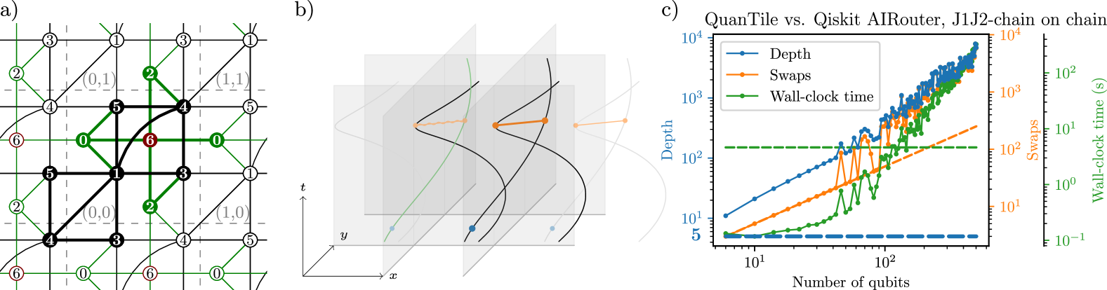
Figure 1: (a) Basis circuit (bold edges) for the quantum simulation of the Kogut-Susskind model of 2D QED. Dashed lines delineate the circuit cells, with their coordinates shown in gray, and seed numbers are indicated within the vertices. The Jordan-Wigner transformation typically breaks 2D spatial periodicity, which we circumvent by using the compact encoding [21], leading to the red auxiliary qubits. (b) Qudit mobility zone. The logical qudits of the basis circuit (black worldlines) are free to move by the action of SWAP gates (omitted) along the edges in a patch of $3\times 3$ hardware cells (edges likewise omitted). The logical qudits are acted upon by single-qudit (dark blue dot) and two-qudit (dark orange edge) physical gates. In this example, the physical circuit (black lines, dark blue dots, and dark orange edges) is repeated to form a $3\times 1$ physical circuit patch. These physical basis circuits interact; a two-qudit gate from a translated copy of the physical basis circuit (wavy orange line) acts between a logical qudit from the original basis circuit and a logical qudit from a translated copy (green line). (c) Benchmarking results comparing QuanTile (dashed lines) with Qiskit’s AIRouter (solid lines).

To overcome restricted qubit connectivity, SWAP gates are commonly inserted [22, 23]. A SWAP gate exchanges the states of two qubits, effectively swapping their positions. To apply a two-qubit gate to a pair of remote qubits, these qubits must be moved (routed) along the edges of the coupling graph using SWAP gates until they become adjacent, at which point the two-qubit gate can be applied. The routing problem [23], also called quantum layout synthesis [24, 25], is the task of determining the initial positions of the qubits and the placement of the SWAP gates. An optimal solution minimizes routing overhead, commonly measured by the routed circuit’s depth or the number of inserted SWAP gates.

Optimal qubit routing is crucial. First, on today’s quantum computers, routing overhead increases the effects of noise, currently limiting simulations to models of quantum magnetism that can be directly embedded into the hardware coupling graph [4, 5, 6, 7]. Second, on early fault-tolerant quantum computers, that have a residual error rate, minimizing routing overhead maximizes the system sizes and simulation times that can be achieved. Finally, while fully scalable fault-tolerant quantum computers can reliably execute circuits of arbitrary depth, especially on cloud-based platforms, the overhead introduced by routing directly increases the monetary cost of running a circuit.

However, solving the routing problem optimally is NP-hard [22, 26, 23]. Although methods for finding optimal solutions exist [24, 27], they are necessarily slow and limited in the circuit sizes they can handle. Recent advances have extended these methods to circuits acting on up to 50 qubits using a highly optimized implementation [28]. However, given the problem’s computational complexity, it is unlikely that optimal routing can be achieved for circuits acting on more than 100 qubits–roughly the number of qubits already available on today’s quantum computers and the scale anticipated to be necessary for a quantum advantage [29, 30]. Consequently, heuristic methods have been developed [31, 23, 32]. While these methods are efficient, they necessarily yield suboptimal solutions, with the SWAP count sometimes exceeding the optimal by several orders of magnitude already on current devices [25].

Spatial periodicity lies at the heart of condensed matter physics. For example, Bloch’s theorem exploits this periodicity to enable the study of infinite systems. Similarly, circuits designed for the quantum simulation of condensed matter systems and lattice gauge theories exhibit a periodic structure: they are composed of a repeated circuit tile, or motif, that recurs both spatially and temporally [33, 34].

In this work, we initiate the study of tileable circuits by focusing on their fundamental circuit tile and leveraging their spatiotemporal periodicity to efficiently achieve optimal routing. We construct several tileable circuits derived from quantum cellular automata [35, 36, 37], condensed matter simulations, and lattice gauge theory simulations, and obtain routing solutions with negligible overhead. This unlocks the potential of today’s quantum computers to study frustrated magnetism and significantly reduces computational cost on fault-tolerant devices.

Our method employs a satisfiability modulo theories (SMT) formulation to solve the routing problem optimally for a single circuit tile while ensuring that the routed circuit remains tileable. Although this problem is still NP-hard, once a solution has been obtained, it can be repeated spatiotemporally at essentially no computational cost. In quantum simulation, this means that the complexity of solving the routing problem depends only on local properties of the simulated system and is essentially independent of the system size and the time for which the system is being simulated.

We implemented our method as an open-source tool, QuanTile [38], with extensive tests of its validity. Benchmarking demonstrates that it can outperform leading general-purpose routing methods on all performance metrics simultaneously. For instance, on a 500-qubit circuit, QuanTile reduces the depth overhead by more than three orders of magnitude while also requiring less computational time; this is possible because QuanTile is a specialized method.

Fundamentals.– We define a circuit tile more formally as a basis circuit (Fig. 1a). It consists of a finite set of gates $g$. A single-qudit gate acts on qudit $g.\tilde{q}$, while a two-qudit gate acts on qudits $g.\tilde{q}$ and $g.\tilde{q}^{\prime}$. (Since the routing problem is independent of whether the degrees of freedom are qubits or qudits with more than two basis states, we use the term ‘qudits’ for generality.) To unambiguously order gates when basis circuits are combined into a circuit patch, we assign each gate a circuit layer $g.\tilde{t}\in\mathbb{N}^{0}$. Each qudit $q$ has cell coordinates $q.\tilde{x},q.\tilde{y}\in\mathbb{Z}$ and a seed number $q.\tilde{s}\in\mathbb{N}^{0}$, which distinguishes qudits within a cell. (This generalizes to higher dimensions by adding spatial coordinates.)

A spatiotemporal circuit patch $P_{n,m,l}(C)$ is formed by merging $n\times m\times l$ translated copies of a depth-$d$ basis circuit $C$,

$$P_{n,m,l}(C)=\bigcup_{\begin{subarray}{c}(\Delta x,\Delta y,\Delta t)\\ \in\,\mathbb{Z}_{n}\times\mathbb{Z}_{m}\times d\,\mathbb{Z}_{l}\end{subarray}}T_{\Delta x,\Delta y,\Delta t}(C).$$ (1)

Here, $T_{\Delta x,\Delta y,\Delta t}(C)$ translates each gate’s time coordinate by $\Delta t$ (i.e., $g.\tilde{t}\mapsto g.\tilde{t}+\Delta t$) and each qudit’s spatial coordinates similarly by $\Delta x$ and $\Delta y$, and $d\,\mathbb{Z}_{l}=\{0,d,2d,\dots,(l-1)d\}$. Replacing $\mathbb{Z}_{n}$ and $\mathbb{Z}_{m}$ with $\mathbb{Z}$ yields spatially infinite, or lattice, circuits. For formal reasons, the union is taken as a multiset union (allowing duplicates). Circuits in which a basis graph can be identified are called tileable circuits.

A gate collision occurs when two gates in the same circuit layer act on the same qudit. A basis circuit $C$ is valid if the circuit patch $P_{n,m,l}(C)$ (or equivalently, its induced lattice circuit) is collision-free for all $n,m,l\in\mathbb{N}^{+}$, which can be checked straightforwardly due to the following theorem.

Theorem 1. Let $C$ be a basis circuit. There are no gate collisions in the circuit patch $P_{n,m,l}(C)$ for all $n,m,l\in\mathbb{N}^{+}$ if and only if, for each time $t$ and seed number $s$, at most one qudit $q$ with $q.\tilde{s}=s$ is acted on by a gate in layer $t$.

Each gate in $P_{n,m,l}(C)$ can be translated back to its source in $C$. A collision in $P_{n,m,l}(C)$ implies that the corresponding source gates in $C$ share the same seed number; conversely, if two gates in the same layer of $C$ act on qudits with the same seed, appropriate translations will lead to a collision in $P_{n,m,l}(C)$. A formal proof is provided in the Supplemental Material (SM) .

In this context, a basis graph [33] can be seen as a basis circuit with edges instead of gates. Edges lack a time coordinate, and two edges may meet at the same vertex. Merging infinitely many translated copies of a basis graph produces a lattice graph, formalizing the concept of an ‘infinite lattice’ with edges. Examples from condensed matter physics include the square, honeycomb, and kagome lattices, with edges connecting nearest neighbors.

Tileable circuits naturally arise in quantum simulations of lattice systems via Trotterization. Consider a two-local Hamiltonian $H=\sum_{i}H_{i}+\sum_{(i,j)}H_{ij}$, acting on $\delta$-dimensional local degrees of freedom (i.e., $\delta$-level qudits), where $H_{i}$ acts on qudit $i$ and $H_{(i,j)}$ on qudits $i$ and $j$ along the edges of a lattice graph $G$. By Trotterization [2, 40], $\mathrm{e}^{-\mathrm{i}\tau H}\approx[\tilde{U}_{p}(\tau/r)]^{r}$, with $\tilde{U}_{p}(\tau/r)$ a $p$th-order Trotter step and $r$ the number of Trotter steps. A first-order step has the form $\tilde{U}_{1}(\tau)=\mathrm{e}^{-\mathrm{i}\tau H^{(1)}}\cdots\mathrm{e}^{-\mathrm{i}\tau H^{(\Gamma)}}$, for some sequence $H^{(1)},\ldots,H^{(\Gamma)}$ of the terms in $H$. Here, $H^{(i)}$ is the $i$th term in the sequence, and each $\mathrm{e}^{-\mathrm{i}\tau H^{(i)}}$ is a two-qudit gate. A second-order Trotter step is constructed by applying the first-order step twice, reversing the order in the second application, $\tilde{U}_{2}(\tau)=\tilde{U}_{1}^{\dagger}(-\tau/2)\,\tilde{U}_{1}(\tau/2)$. Using the bounds from [40], the error is $O\bigl{[}N\tau\,(\tau/r)^{p}\bigr{]}$, where $N$ is the number of qudits. Importantly, $\tilde{U}_{p}$ is tileable for any $p$. For the routing problem, only the structure of $G$ matters, so we consider arbitrary two-local (ATL) Hamiltonians, including models such as the Ising, (an)isotropic Heisenberg, Kitaev, and Bose-Hubbard models [39]. Trotterization does not prescribe a specific order $H^{(i)}$. Finding the order that minimizes circuit depth is equivalent to solving an NP-hard edge-coloring problem [33]. We finally note that tileable circuits also arise naturally in the task of finding ground states of lattice systems, for example, because the implementation of $\mathrm{e}^{-\mathrm{i}\tau H}$ is a core subroutine [41], or because $\tilde{U}_{1}$ determines the structure of a parameterized ansatz circuit [42, 43].

Routing.– It is common to call the circuit to be routed the logical circuit, acting with logical gates on logical qudits. The routed circuit is the physical circuit, acting with physical gates on physical qudits, while respecting hardware connectivity constraints. Although qudit routing is also needed for fault-tolerant quantum computing, the terms logical and physical here differ from their usage in error correction, where a single logical qudit is encoded into multiple physical qudits.

To execute a logical circuit on the hardware available, each logical qudit $q$ is assigned to a physical qudit $Q$ via a logical-to-physical qudit map $Q_{q}$, or qudit map for short. We say the logical qudit $q$ resides at the physical qudit $Q_{q}$. SWAP gates are inserted to ensure logical gates can be performed within the connectivity constraints. If $q$ starts at $Q_{q}$ and a SWAP acts on $Q_{q}$ and $Q^{\prime}$, then afterward $q$ resides at $Q^{\prime}$. The qudit map has to be updated accordingly.

The routing problem for standard circuits was formulated as an SMT formula in [24]. An SMT formula consists of variables and constraints. Here, Boolean and integer variables encode the qudit map, the coordinates of the physical qudits of gates, and the time coordinates of physical gates. Constraints on those variables ensure that the corresponding physical circuit is without gate collisions, respects the hardware connectivity, implements the same unitary as the logical circuit (up to a final reordering of the qudits), and has a preset depth $D>0$. The smallest $D$ for which all constraints become satisfiable yields the routed circuit with minimal depth overhead.

The second-order Trotter formula (and higher-order versions [39]) offers an advantage in qudit routing. Let $U(\tau)$ be the routed version of $\tilde{U}_{1}(\tau)$. At the end of $U(\tau)$, logical qudits may not return to their initial positions, but after $U^{\dagger}(-\tau)U(\tau)$, they do. Thus, $\mathrm{e}^{-i\tau H}\approx[\tilde{U}_{2}(\tau/r)]^{r}=[U^{\dagger}(-\tau/(2r))U(-\tau/(2r))]^{r}$, where the right-hand side is a fully routed circuit. To route $r$ repetitions of a second-order Trotter step, it suffices to route a single first-order step without enforcing logical qudits to return to their initial position. This temporal periodicity can be exploited alongside spatial periodicity. Alternatively, one can enforce qudits to return to their initial positions at the end of $U(\tau)$, though this may increase circuit depth.

When simulating Hamiltonians with two-qubit interactions of the form $H_{ij}(\Delta)\sim X_{i}X_{j}+Y_{i}Y_{j}+\Delta Z_{i}Z_{j}$ on hardware where the native two-qubit gate is the CNOT, SWAP gates can be absorbed into directly preceding or following two-qubit simulation unitaries $\mathrm{e}^{-\mathrm{i}\tau H^{(i)}}$ at no increase of the infidelity of the subcircuits implementing those unitaries [39]. The same applies when the native two-qubit gate is the fSim gate [44, 39].

Simulated	Hardware	Depth	SWAP
system	coupling graph	overhead	overhead
ATL ladder	chain	0 (0 %)	0
ATL J1J2-ladder	chain	0 (0 %)	0
ATL J1J2-chain	chain	1 (25 %)	0
Rule 54	ladder	0 (0 %)	1 (4)
ATL J1J2-chain	ladder	0 (0 %)	0
ATL J1J2-square	square grid	0 (0 %)	0
ATL triangular	square grid	0 (0 %)	0
ATL kagome	square grid	1 (25 %)	0
ATL shuriken	square grid	1 (25 %)	0
ATL snub-square	square grid	1 (20 %)	0
Rokhsar-Kivelson	square grid	2 (11 %)	2 (4)
Fermi-Hubbard	square grid	0 (0 %)	0
Kogut-Susskind	square grid	9 (4 %)	253 (6)

Table 2: Excerpt of the results obtained by QuanTile in routing a single Trotter step for various lattice systems (first column) to various hardware coupling lattice graphs (second column). ATL J1J2-$\ell$ stands for an arbitrary two-local model (ATL) on a lattice $\ell$ with edges between nearest and next-nearest neighbors. The reported depth overhead (third column) is given per Trotter step and remains valid for any number of Trotter steps and logical circuit patch size. The SWAP overhead (last column) is specified per Trotter step and per the number of qudits indicated in parentheses. In all listed solutions, the qudit overhead is zero, except for Kogut-Susskind, where it is one qudit per seven logical qudits.

Routing tileable circuits.– To leverage spatial periodicity, we optimally route logical basis circuits to physical basis circuits. In other words, we map tileable circuits to hardware whose connectivity graph is described by (a patch of) a lattice graph. The unitary implemented by any $n\times m\times l$ physical circuit patch must equal (up to a possible reordering of qudits defined by the final qudit map) the unitary implemented by the corresponding $n\times m\times l$ logical circuit patch. Since this holds for any $n$ and $m$, we may even consider infinite physical circuit patches, or physical lattice circuits.

In the mathematical formulation of the qudit routing problem for tileable circuits, several concepts and assumptions beyond those required for standard routing are essential. Most importantly, when placing any gate into the physical basis circuit, we must ensure that no gate collisions occur in any physical circuit patch induced by the physical basis circuit [Eq. (7)]. This is done straightforwardly by using Theorem 1, demonstrating its necessity and effectiveness.

Second, due to the discrete spatial translational symmetry of a physical lattice circuit, the qudit map must share the same symmetry. Therefore, we assume that the initial qudit map conserves cell coordinates. Translational symmetry then requires that for each seed number $s$, there is a unique seed number $S$ such that all logical qudits with seed number $s$ are mapped to physical qudits with seed number $S$. We also assume that the physical basis circuit fits within the mobility zone, a patch of $3\times 3$ hardware cells (Fig. 1b). Logical qudits can move along the edges of the hardware lattice graph via SWAP gates, but they cannot leave the mobility zone. The size of the mobility zone can be increased at the cost of additional computational resources.

Finally, consider inserting a SWAP gate $g$ acting on physical qudits $(Q,Q^{\prime})$ into the physical basis circuit $C$. By Eq. (7), the physical lattice circuit induced by $C$ will include SWAP gates along $T_{\Delta x,\Delta y,0}[g]$ for every $\Delta x,\Delta y$. Crucially, these translated SWAP gates, although they are not in $C$ itself, may generally act on physical qudits of $C$ holding logical qudits. We account for this effect by temporarily inserting all relevant possible translated versions of each SWAP gate that is added to the physical basis circuit. This renders the basis circuit technically invalid by Theorem 1. In post-processing, however, we retain only the untranslated SWAP gate, ensuring that no collisions occur in the physical lattice circuit. The translated SWAP gates acting on $C$ automatically reemerge in the final physical lattice circuit.

In an independent implementation based on [24], we reformulated the above as an SMT formula, which can be found in full in the SM [39]. It provides the following additional options that, like tileability, go beyond the capabilities of standard routing methods: (i) optimize the order of two-qudit gates in the Trotter step; (ii) allow SWAP gates to merge with directly preceding or following two-qudit gates; (iii) enforce that logical qudits return to their initial positions at the end of the circuit (‘cyclic routing’); and (iv) slice the logical circuit into subcircuits to route sequentially, reducing the computational complexity to linear in the logical circuit depth.

Results.– We applied QuanTile to basis circuits for one Trotter step in the quantum simulation of ATL Hamiltonians on 24 different 1D and 2D lattices. Additionally, we considered the Fermi-Hubbard model on the square lattice [10], the Rokhsar-Kivelson model [12], and the Kogut-Susskind model of 2D QED [13]. Finally, we applied QuanTile to the basis circuit of the Rule 54 quantum cellular automaton [36, 37]. By using Eq. (7), the solutions can be tiled spatially and temporally, creating arbitrarily deep and wide routed circuits. The routing problems were solved for various combinations of the routing options (i–iv). All circuits and the 1D and 2D lattices are provided explicitly in the SM, along with extensive results [39].

An excerpt of the results is given in Table 1, with the following routing options. For the ATL models only, we optimized the gate order (i). We allowed SWAP-merging (ii), except for the Fermi-Hubbard circuit. We enforced cyclic routing (iii), except for the ATL circuits. Logical circuits were not sliced (iv), except for the Kogut-Susskind circuit, which had a slice depth of 20. For the solutions we found, the routing overhead is remarkably low. In some cases there is no overhead at all, possible under option (i).

QuanTile offers a scaling advantage over general-purpose methods because its running time is essentially independent of the logical circuit size. Nevertheless, the question remains if this advantage already plays a significant role for today’s quantum chips, with on the order of a hundred to a thousand qubits.

We therefore benchmarked QuanTile against multiple established routing methods across various routing problems. The full benchmarking data, including details on the implementations and the hardware, are provided in the SM [39]. Here, we show the results of comparing QuanTile to Qiskit’s leading AIRouter [32] on the problem of routing a single Trotter step (for both methods) of an ATL J1J2 model on a chain to hardware with chain connectivity (Fig. 1c). Since the AIRouter does not optimize gate order (i), we allow QuanTile to perform this optimization and then use the resulting gate order as a fixed input for the AIRouter. Because the AIRouter does not support SWAP merging (ii) or cyclic routing (iii), we disable these options in QuanTile. As both methods route a single Trotter step, their solutions can be repeated temporally to construct arbitrarily deep second-order Trotter circuits, but only QuanTile’s solution can also be repeated spatially.

QuanTile’s improved scaling behavior makes it faster for system sizes above approximately 100 qudits, while also producing solutions with significantly lower depth and SWAP overhead. At around 500 qudits, the depth overhead decreases from approximately $10^{4}$ to just 5.

Conclusion.– Quantum simulation holds great promise as an application of quantum computing, but leading experiments are significantly limited by the overhead arising from device connectivity constraints. We have demonstrated that for spatiotemporal periodic circuits – naturally arising in the quantum simulation of condensed matter systems and lattice gauge theories – inherently scalable routing solutions can be achieved with negligible overhead.

Beyond reducing costs on fault-tolerant devices, our routing solutions enable the simulation of geometrically frustrated magnetism on current devices. One possibility is the observation of disorder-free localization and many-body quantum scars in a Heisenberg model on the kagome lattice [45, 46]. The circuits require $O(1)$-depth state preparation, followed by the Trotterized simulation circuit, which for this system is possible on square-grid hardware using five fSim gate layers per Trotter step (Table 1). With 100 qubits and a depth-100 circuit, which could be within reach of pre-fault tolerant devices [30], it becomes possible to simulate around 11 second-order (or 17 first-order [39]) Trotter steps on 100 qubits.

A highly optimized implementation of QuanTile is expected to decrease running times by several orders of magnitude [28]. Also, while our focus has been on an optimal method, we anticipate that heuristic methods can also be adapted so that their solutions are tileable. This could be valuable when the basis circuits become too large for optimal methods, e.g., when routing circuits for future modular and tileable hardware, where each module consists of hundreds of qubits [47].

Although our emphasis has been on the routing problem, we have laid the foundation for addressing other compilation tasks in the tileable setting. Examples include leveraging gate identities to reduce logical circuit depth [48] and automated and optimized construction of quantum simulation circuits [49]. Exploiting tileability, similar improvements over leading methods are expected in these areas as well.

Data availability

QuanTile and all data are available open-source at [38].

Supplemental material to:

“Optimal and efficient qubit routing for quantum simulation”

I Fundamental concepts

Here, we formally introduce concepts fundamental for defining and routing tileable circuits, as well as for constructing tileable hardware connectivity graphs. These correspond to the definitions in quantile/base.py in the implementation [38].

I.1 Basis graphs

A basis graph $B$ is a graph $B=(V(B),E(B))$ with vertex set $V(B)$ and edge set $E(B)$. Each vertex $v\in V(B)$ has the form $v=(v_{x},v_{y},v_{s})$, where $v_{x},v_{y}\in\mathbb{Z}$ are cell coordinates, and $v_{s}\in\mathbb{N}^{0}$ is an identifier called the seed number of the vertex. For clarity, we assume two-dimensional basis graphs; higher-dimensional basis graphs can be obtained by extending the list of cell coordinates accordingly.

Basis graphs (along with lattice graphs) were formally introduced in Ref. [33]. However, we present their definitions here in a slightly different but equivalent form for completeness and consistency with the definitions of basis circuits. For a visual example of basis and lattice graphs, we refer the reader to Fig. 1 of Ref. [33].

We define the translation operator on vertices as $T_{\Delta x,\Delta y}(v)=(v_{x}+\Delta x,v_{y}+\Delta y,v_{s})$. This naturally extends to a translation operator on an edge $e=(e_{0},e_{1})$ by applying $T$ to each of its vertices, $T_{\Delta x,\Delta y}(e)=(T_{\Delta x,\Delta y}(e_{0}),T_{\Delta x,\Delta y}(e_{1}))$. For simplicity of notation, we use $T$ to denote the translation operator on both vertices and edges. Extending this definition further, $T$ induces a translation operator on basis graphs by applying $T$ to all vertices and edges in the graph, $T(B)=(T[V(B)],T[E(B)])$, where $T[E(B)]$ is the set obtained by applying $T$ to each edge in $E(B)$ separately, and similarly for $T[V(B)]$.

A lattice graph $\mathcal{G}$ is obtained by translating and merging infinitely many copies of a basis graph $B$,

$$\mathcal{G}(B)=\bigcup_{\Delta x,\Delta y\in\mathbb{Z}}T_{\Delta x,\Delta y}(B).$$ (2)

The union of two graphs $A$ and $B$ is defined as $A\cup B=\big{(}V(A)\cup V(B),E(A)\cup E(B)\big{)}$. A patch of a lattice graph is a finite subgraph obtained by translating and merging a bounded number of copies of $B$,

$$P_{n,m}(B)=\bigcup_{\Delta x\in\mathbb{Z}_{n},\Delta y\in\mathbb{Z}_{m}}T_{\Delta x,\Delta y}(B).$$ (3)

A cell at coordinates $(x,y)$ consists of all vertices in $V(\mathcal{G})$ that share the same cell coordinates $(x,y)$. We refer to the cell at $(x,y)=(0,0)$ as the central cell.

I.2 Basis circuits

Similar to a basis graph, a basis circuit $C=(Q(G),G(C))$ with qudits $Q(C)$ and gates $G(C)$ is a circuit in which each qudit $q$ has a cell $x$-coordinate $q.\tilde{x}$, a cell $y$-coordinate $q.\tilde{y}\in{\mathbb{Z}}$ and a seed number $q.\tilde{s}\in\mathbb{N}^{0}$. We denote the qudit a single-qudit gate $g\in G(C)$ acts on by $g.{\tilde{q}}$. For two-qudit gates, we denote the qudits the gate acts on by $g.{\tilde{q}}$ and $g.{\tilde{q}^{\prime}}$. To ensure an unambiguous gate order when using a basis circuit to generate a circuit patch, we explicitly include the circuit layer (or time step) at which each gate $g$ operates, denoted by $g.\tilde{t}\in\mathbb{N}^{0}$. In Sec. I.5, we demonstrate that if gate times are unspecified, they can always be assigned while preserving tileability and wile utilizing gate parallelism.

Similar to vertices, we define the translation operator acting on a qudit $q$ as $T_{\Delta x,\Delta y}(q)=q^{\prime}$, with $q^{\prime}.\tilde{x}=q.\tilde{x}+\Delta x$, $q^{\prime}.\tilde{y}=q.\tilde{y}+\Delta y$, and $q^{\prime}.\tilde{s}=q.\tilde{s}$. This naturally induces a translation operator on gates by translating each qudit that a gate $g$ acts on by the same amount. That is, for the translated gate $T_{\Delta x,\Delta y,\Delta t}(g)=g^{\prime}$, we have $g^{\prime}.\tilde{q}=T_{\Delta x,\Delta y}(g.\tilde{q})$. For two-qudit gates, we additionally have $g^{\prime}.\tilde{q}^{\prime}=T_{\Delta x,\Delta y}(g.\tilde{q}^{\prime})$. Furthermore, the time coordinate transforms as $g^{\prime}.\tilde{t}=g.\tilde{t}+\Delta t$. The translation operator on gates induces a translation operator on basis circuits by translating each gate and qudit in the circuit; $T_{\Delta x,\Delta y,\Delta t}(C)=(T_{\Delta x,\Delta y}(Q(C)),T_{\Delta x,\Delta y,\Delta t}(G(C)))$, where $T_{\Delta x,\Delta y}(Q(C))$ translates each qudit in $Q(C)$, and $T_{\Delta x,\Delta y,\Delta t}(G(C))$ translates each gate in $G(C)$.

Continuing the analogy to graphs, a (finite-depth) lattice circuit $\mathcal{C}$ is obtained by translating and merging infinitely many copies of a basis circuit $C$. That is,

$$\mathcal{C}(C)=\bigcup_{\Delta x,\Delta y\in\mathbb{Z}}T_{\Delta x,\Delta y}(C).$$ (4)

The union of two circuits $A$ and $B$ is defined as $A\cup B=(Q(A)\cup Q(B),G(A)\cup G(B))$. A patch of a lattice circuit is obtained by translating and merging a finite number of copies of a basis circuit $C$,

$$P_{n,m}(C)=\bigcup_{\Delta x\in\mathbb{Z}_{n},\Delta y\in\mathbb{Z}_{m}}T_{\Delta x,\Delta y,0}(C).$$ (5)

A circuit cell at $(x,y)$ consists of all qudits in $Q(C)$ that have cell coordinates $(x,y)$. The circuit layer $t$ of a basis circuit, circuit patch, or lattice circuit consists of all gates $g$ in that circuit for which $g.\tilde{t}=t$. The depth $d$ of a basis circuit, circuit patch, or lattice circuit is the number of layers in the circuit.

Quantum circuits for quantum simulation via Trotterization (Sec. II) consist of a circuit cycle that is repeated temporally. For this application, it is natural to consider circuits that are periodic in time and define spacetime patches as

$$P_{n,m,l}(C)=\bigcup_{\Delta x\in\mathbb{Z}_{n},\Delta y\in\mathbb{Z}_{m},\Delta t\in d\,\mathbb{Z}_{l}}T_{\Delta x,\Delta y,\Delta t}(C),$$

where $d\,\mathbb{Z}_{l}$ denotes $\{0,d,2d,\ldots,d(l-1)\}$, with $d$ the depth of $C$.

Unlike edges, two gates may not collide. A gate collision between two gates $g,g^{\prime}\in G(C)$ occurs if $g.\tilde{t}=g^{\prime}.\tilde{t}$ and there exist qudits $\tilde{a}$ and $\tilde{b}$ such that $g.\tilde{a}=g^{\prime}.\tilde{b}$, where $\tilde{a}\in\{\tilde{q}\}$ for single-qudit gates and $\tilde{a}\in\{\tilde{q},\tilde{q}^{\prime}\}$ for two-qudit gates, with $\tilde{b}$ satisfying a similar condition. Gate collisions cannot occur in $C$ if $C$ is a valid quantum circuit. Moreover, gate collisions should not arise when generating a lattice circuit or any circuit patch. Therefore, for $C$ to qualify as a basis circuit, we require that no gate collisions occur in $P_{n,m,l}(C)$ for any $n,m,l\in\mathbb{N^{+}}$. A necessary and sufficient condition for this property is that in each layer of the circuit, at most one qudit with seed number $s$ is acted upon by a gate in that layer.

Theorem 1.

Let $C$ be a basis circuit. There are no gate collisions in the circuit patch $P_{n,m,l}(C)$ for arbitrary $n,m,l\in\mathbb{N}^{+}$ if and only if, for every time $t$ and seed number $s$, there is at most one qudit $q\in Q(C)$ acted on by layer $t$ of $C$ so that $q.\tilde{s}=s$.

Proof.

By construction of $P_{n,m,l}$, there cannot be gate collisions due to temporal translation and hence in the following we may take $l=1$. Suppose there exist $n,m,l\in\mathbb{N}^{+}$ for which a gate collision occurs in $P_{n,m,l}(C)$. Then there exists a layer $t$ and a qudit $q$ such that two distinct gates $g,g^{\prime}\in G(C)$, both acting in layer $t$, operate on $q$. By the construction of $P_{n,m,l}(C)$, there exist translations $(\Delta x,\Delta y)$ and $(\Delta x^{\prime},\Delta y^{\prime})$ such that $g=T_{\Delta x,\Delta y}(\mathfrak{g})$ and $g^{\prime}=T_{\Delta x^{\prime},\Delta y^{\prime}}(\mathfrak{g}^{\prime})$ for some $\mathfrak{g},\mathfrak{g}^{\prime}\in G(C)$. Note that $(\Delta x,\Delta y)\neq(\Delta x^{\prime},\Delta y^{\prime})$, since if they were equal a gate collision would already occur in $C$, contradicting its validity. Applying the corresponding translations to $q$, we obtain $q=T_{\Delta x,\Delta y}(\mathfrak{q})$ and $q=T_{\Delta x^{\prime},\Delta y^{\prime}}(\mathfrak{q}^{\prime})$ with $\mathfrak{q},\mathfrak{q}^{\prime}\in Q(C)$ and $\mathfrak{q}\neq\mathfrak{q}^{\prime}$. Since these translations yield the same qudit $q$, it follows that $\mathfrak{q}.\tilde{s}=\mathfrak{q}^{\prime}.\tilde{s}$.

Conversely, assume that there exist a time $t$, a seed number $s$, and distinct qudits $q,q^{\prime}\in Q(C)$, both acted on by layer $t$ of $C$, such that $q.\tilde{s}=q^{\prime}.\tilde{s}=s$. Then there exist $\Delta x,\Delta y\in\mathbb{Z}$ such that $T_{\Delta x,\Delta y}(q^{\prime})=q$. Consider the circuit layer $t$ of the translated circuit $T_{\Delta x,\Delta y}(C)$. Since $q^{\prime}\in Q(C)$, this layer acts on the qudit $T_{\Delta x,\Delta y}(q^{\prime})=q$. Hence, both $C$ and $T_{\Delta x,\Delta y}(C)$ act on qudit $q$ in layer $t$, which implies that there exist integers $n,m$ for which the circuit patch $P_{n,m,l}(C)$ contains a gate collision. ∎

I.3 Tileable circuits

In this work, a tileable circuit refers to the informal notion of a circuit intended for spatial and/or temporal repetition. When all qudits of a circuit patch or basis circuit are mapped to integers, the resulting circuit is formally no longer a circuit patch or basis circuit. Additionally, circuits that lead to full gate collisions may still be considered tileable circuits. In such cases, it is implicitly understood that, depending on the context, these full gate collisions are resolved either by retaining only one of the colliding gates upon spatial repetition or by merging the two gates into a single operation. A gate collision between two gates $g$ and $g^{\prime}$ is considered full if the sets of qudits acted upon by $g$ and $g^{\prime}$ are identical. Moreover, a circuit may be described as tileable or composed of circuit tiles even before explicitly identifying the specific basis circuit that will be repeated.

I.4 Reseeding

In the remainder of this work, we will always route basis circuits to hardware with a connectivity graph generated by a basis graph. However, the number of seed numbers of the basis graph (usually equal to the number of vertices in the central cell of the basis graph) may significantly exceed the number of seed numbers in the basis circuit, or vice versa. Moreover, we anticipate that the quality of the routing solution generally improves when large circuit patches are mapped onto correspondingly large hardware patches. Consequently, we seek a general approach for routing circuit patches $P_{n,m,l}(C)$ to hardware generated by patches $P_{n^{\prime},m^{\prime}}(B)$ while ensuring that the solution can be tiled.

However, in formulating the routing problem for tileable circuits as a satisfiability modulo theories (SMT) problem (Sec. V) and in Theorem 1, it is significantly more convenient to focus on basis graphs and basis circuits exclusively. Additionally, we have not yet established a formal method for generating lattice graphs from patches or lattice circuits from circuit patches. Fortunately, any lattice graph patch $P_{n^{\prime},m^{\prime}}(B)$ can be transformed into a basis graph via a process known as reseeding [33]. A similar approach applies to circuit patches.

The key idea behind reseeding a hardware patch $P_{n^{\prime},m^{\prime}}(B)$ generated by a basis graph $B$ is to assign a unique seed number $s^{\prime}(v)$ to each vertex $v$ in $P_{n^{\prime},m^{\prime}}(B)$ that satisfies $0\leq v_{x}<n^{\prime}$ and $0\leq v_{y}<m^{\prime}$, and then map these vertices to $v^{\prime}=(0,0,s^{\prime}(v))$. This effectively places the vertices in the central cell of a new basis graph. Vertices $v$ that fall outside the range $0\leq v_{x}<n^{\prime}$ and $0\leq v_{y}<m^{\prime}$ must be mapped accordingly. The explicit details of this procedure are provided in Ref. [33]. Reseeding a circuit patch is essentially the same as reseeding a lattice graph patch; all qudits have to be updated according to essentially the same procedure.

I.5 Gate scheduling

Quantum circuits are typically represented as an ordered list of gates, without explicitly specifying the time steps at which the gates should be executed. From this list, a valid time assignment can be obtained by scheduling the $i$the gate, $g^{(i)}$, at time step $i$. However, this results in unnecessarily deep circuits, as no gates are performed in parallel. A method that leads to shallower circuits is to place each gate as early as possible. Intuitively, this can be visualized as follows. Consider the circuit diagram and iteratively move each gate to the left until it encounters another gate that prevents further movement. This process continues until no gate can be shifted leftward. The resulting diagram is then partitioned into slices, each representing a layer of depth 1, with all gates in slice $i$ assigned to time step $i$.

However, directly applying this approach to basis circuits leads to invalidly scheduled basis circuits, as collisions may arise when the basis circuit is used to generate a circuit patch. To address this, we first impose periodic boundary conditions on the basis circuit. This is accomplished by setting $g.\tilde{q}.\tilde{x}=g.\tilde{q}.\tilde{y}=0$ (and similarly for $\tilde{q}^{\prime}$) for all gates $g$ in the circuit. After imposing the periodic boundary conditions, we then schedule the gates by assigning each gate $g$ to the earliest possible time $g.t$. Finally, we revert all qudits to their original values. This process is depicted in Fig. 2.

In defining a specific basis circuit, it is often less confusing to explicitly specify the times at which gates in the basis circuit should be executed, rather than providing a list of gates without any time assignments. However, the resulting basis circuit may not always fully exploit gate parallelizability. In such cases, the process outlined above can be applied to reduce the circuit depth, and in this context, the process is more accurately referred to as gate rescheduling.

Figure 2: Gate scheduling. (a) A basis circuit is specified as a list of gates. Dashed lines delineate the central cell of the basis circuit. In this example, the basis circuit is defined on a 1D chain. (b) Treating the basis circuit as a standard circuit results in incorrect gate scheduling; the depicted circuit leads to gate collisions when the circuit is used to generate a circuit patch. (c) The correct scheduling method is to first impose periodic boundary conditions on the circuit. In this picture, time runs radially outward in integer steps. Gates are assigned times accordingly. (d) Periodic boundary conditions are lifted, yielding the correctly scheduled basis circuit.

I.6 Gate dependencies

A gate dependency $(A,B)$ indicates that gate $A$ must be executed before gate $B$. When routing a circuit, the gate dependencies of the input circuit need to be respected in the output circuit as well (unless they explicitly do not need to be respected, as is the case when gates commute or in Trotterized quantum simulation circuits). In tileable circuits, identifying dependencies requires special attention. For example, considering the circuit in Fig. 2a as a standard circuit, there is no dependency between the two-qudit gates $g^{(1)}$ (the first gate) and $g^{(3)}$ (the third gate). However, when treating it as a basis circuit, we have the dependency $(g^{(1)},g^{(3)})$. This dependency becomes apparent only in the wrapped circuit [Fig. 2c].

To extract gate dependencies from the wrapped basis circuit, we use its directed acyclic graph (DAG) representation (Fig. 3) of circuits. In this representation, gates correspond to vertices. Each vertex has incoming edges labeled with the qudits the gate acts on and outgoing edges labeled with the qudits it has acted on. The edges labeled with qudit $q$ are sourced from a vertex $\mathrm{source}_{q}$ and terminate at a sink vertex $\mathrm{sink}_{q}$. The DAG representation can be viewed as a formalized version of standard quantum circuit diagrams, where the absolute positioning of objects carries no intrinsic meaning.

Figure 3: DAG representation of the circuit in Fig. 2c. Source nodes are white, and sink nodes are gray. Each gate node also displays the qudits it acts on as an ordered list. This information is necessary; otherwise, it would be impossible to determine, for example, in the case of a CNOT gate, which of the two incoming edges represents the control qudit and which represents the target qudit.

Denote the $j$th gate in the basis circuit by $g^{(j)}$ and its counterpart after imposing periodic boundary conditions by $g^{(j)^{\prime}}$. From the DAG of the wrapped basis circuit, we iterate through all gates $g^{(j)^{\prime}}$. For each $g^{(j)^{\prime}}$, we add to a dependency list all pairs $(g^{(i)},g^{(j)})$ such that $g^{(i)^{\prime}}$ is a parent of $g^{(j)^{\prime}}$ in the DAG. The dependency list thus contains only the ‘direct’ dependencies. However, since gate dependency is transitive, ensuring that direct dependencies are respected in the routed circuit guarantees that all gate dependencies are respected.

II Tileable circuits from Trotterization

Consider a Hamiltonian

$$H=\sum_{i_{1},\ldots,i_{n}}H_{i_{1},\ldots,i_{k}},$$ (6)

where each term $H_{i_{1},\ldots,i_{k}}$ acts on $k$ degrees of freedom $(i_{1},\ldots,i_{k})$ defined on a Bravais lattice. Assume that $H$ is geometrically local, meaning that for any nonzero term $H_{i_{1},\ldots,i_{k}}$, the indices $i_{1},\ldots,i_{k}$ lie within a neighborhood where the maximum distance between any two degrees of freedom $i_{j}$ and $i_{l}$ is independent of system size. We assume this neighborhood corresponds to a supercell of $3\times 3$ unit cells in two dimensions or $3^{D}$ unit cells in general dimension $D$. This assumption is without loss of generality because, given the geometric locality of $H$, the unit cell size can always be enlarged until the neighborhood fully contains all degrees of freedom within a fixed radius.

In quantum simulation by Trotterization, the system size is fixed to $n$ degrees of freedom, leading to the Hamiltonian

$$H=\sum_{\gamma}^{\Gamma}H_{\gamma}$$ (7)

for some ordering $(H_{1},\ldots,H_{\Gamma})$ of the terms in Eq. (6), where $H_{\gamma}$ denotes the $\gamma$th term in this ordering. An approximation $[\tilde{U}_{p}(t/r)]^{r}$ of the time-evolution unitary $U(t)=\mathrm{e}^{-itH}$ is applied to an initial state. (Throughout, we use units where $\hbar=1$.) Here, $p$ determines the order of the approximation, and $r$ is the number of Trotter steps.

The first-order Lie-Trotter approximation is given by

$$\tilde{U}_{1}(t)=\mathrm{e}^{-\mathrm{i}tH_{1}}\ldots\mathrm{e}^{-\mathrm{i}tH_{\Gamma}}.$$ (8)

Higher-order Suzuki formulas are defined recursively as

$$\tilde{U}_{2}(t) =\mathrm{e}^{-\mathrm{i}\frac{t}{2}H_{\Gamma}}\ldots\mathrm{e}^{-\mathrm{i}\frac{t}{2}H_{1}}\mathrm{e}^{-\mathrm{i}\frac{t}{2}H_{1}}\ldots\mathrm{e}^{-\mathrm{i}\frac{t}{2}H_{\Gamma}},$$ (9)

$$\tilde{U}_{2\ell}(t) =[\tilde{U}_{2\ell-2}(u_{\ell}t)]^{2}\tilde{U}_{2\ell-2}[(1-4u_{\ell})t][\tilde{U}_{2\ell-2}(u_{\ell}t)]^{2},$$

with $\tilde{U}_{2\ell-1}(t)=\tilde{U}_{2\ell}(t)$ and $u_{\ell}=1/[4-4^{1/(2\ell-1)}]$ [50]. We refer to $\tilde{U}_{p}(t)$ (for any $p=1,2,4,\ldots$) as a Trotter step. Notably, $[\tilde{U}_{p}({\textstyle\frac{t}{r}})]^{r}$ consists of $k$-body gates, each of which can be compiled into a number of two-body gates independent of $n$. Given $H$ as in [Eq. (6)], then the circuit $[\tilde{U}_{p}(t)]^{r}$ tileable (and can hence be described as a patch of a lattice circuit).

In Ref. [40], it was shown that

$$\lVert\tilde{U}_{p}(t)-\mathrm{e}^{-\mathrm{i}tH}\rVert=O(\lvert\hskip-1.00006pt\lvert\hskip-1.00006pt\lvert H\rvert\hskip-1.00006pt\rvert\hskip-1.00006pt\rvert^{p}_{1},\lVert H\rVert_{1}t^{p+1}),$$ (10)

where

$$\lvert\hskip-1.00006pt\lvert\hskip-1.00006pt\lvert H\rvert\hskip-1.00006pt\rvert\hskip-1.00006pt\rvert_{1}=\max_{l}\max_{i_{l}}\sum_{i_{1},\ldots,i_{l-1},i_{l+1},\ldots,i_{k}}\lVert H_{i_{1},\ldots,i_{k}}\rVert,$$ (11)

with $\|\cdot\rVert$ denoting the operator norm, and

$$\lVert H\rVert_{1}=\sum_{\gamma}\lVert H_{\gamma}\rVert.$$ (12)

The sum in $\lvert\hskip-1.00006pt\lvert\hskip-1.00006pt\lvert H\rvert\hskip-1.00006pt\rvert\hskip-1.00006pt\rvert_{1}$ implicitly only includes terms also appearing in Eq. (7).

We now consider what this implies lattice circuits. Note that, due to locality, $\lvert\hskip-1.00006pt\lvert\hskip-1.00006pt\lvert H\rvert\hskip-1.00006pt\rvert\hskip-1.00006pt\rvert_{1}=O(1)$ and $\lVert H\rVert_{1}=O(n)$. Using the inequality

$$\lVert[\tilde{U}_{p}(t/r)]^{r}-\mathrm{e}^{-\mathrm{i}tH}\rVert\leq r\lVert\tilde{U}_{p}(t/r)-\mathrm{e}^{-\mathrm{i}\frac{t}{r}H}\rVert,$$ (13)

the error from applying the $p$th-order Suzuki formula becomes

$$\lVert[\tilde{U}_{p}(t/r)]^{r}-\mathrm{e}^{-\mathrm{i}tH}\rVert=O\left[nt\left({\textstyle\frac{t}{r}}\right)^{p}\right].$$ (14)

This bound can be made arbitrarily close to $O(nt)$ by increasing $p$, but note that increasing $p$ also increases the number of gates required for a single Trotter step.

In qudit routing, the temporal periodicity, or cyclicity, of the circuit $[\tilde{U}_{p}(t/r)]^{r}$ can be directly exploited. One first routes the circuit $\tilde{U}_{p}(t/r)$ and then repeats the routed version $r$ times. The only requirement is that the logical qudits $q$ return to their initial positions after the final layer of the routed circuit $\tilde{U}_{p}(t/r)$. (In our implementation [38], this can be achieved by setting the transpiler option cyclic = True.)

Higher-order Suzuki formulas provide an advantage in routing. The second-order Suzuki formula consists of two applications of the first-order formula, where the second application has the reversed gate order. We may write this as

$$\tilde{U}_{2}(t)=\tilde{U}_{1}^{\dagger}(-t/2)\tilde{U}_{1}(t/2).$$ (15)

If $C(t)$ is the routed version of $\tilde{U}_{1}(t/2)$ (where the logical qudits need not return to their initial positions), then in the circuit $C^{\dagger}(-t/r)C(t/r)$ the logical qudits do return to their initial positions. Therefore, when routing $[\tilde{U}_{2}(t/r)]^{r}$, it suffices to route $\tilde{U}_{1}(t/r)$ without enforcing that the logical qudits return to their initial positions. That is,

$$[\tilde{U}_{2}(t/r)]^{r}=[C^{\dagger}(-t/r)C(t/r)]^{r}.$$ (16)

More generally, the same alternating structure of $\tilde{U}_{1}$ and its reversed circuit persists for any Suzuki order $p$. Thus, to route $r$ repetitions of $p$th order Trotter step, it suffices to route $\tilde{U}_{1}$, independent of $r$ and $p$, and without the need of imposing that the logical qudits return to their initial positions.

III Merging SWAP gates

In this work, we do not assume a specific type of quantum hardware. As in Ref. [34], we therefore adopt a costing model in which each general two-qudit gate has unit cost. In particular, this implies that any SWAP gate immediately preceding (following) a two-qudit unitary $U_{ij}$ acting on the same two qudits can be merged into that unitary, yielding a new unitary $U^{\prime}_{ij}=U_{ij}\,\mathrm{SWAP}$ ($U^{\prime}_{ij}=\mathrm{SWAP}\,U_{ij}$) that has unit cost.

We emphasize that in the formulation of the routing problem as an SMT formula, it is entirely possible to go beyond this costing model by incorporating additional details about the hardware, if necessary. For instance, Ref. [24] considers a scenario where a SWAP gate requires three units of time.

Nevertheless, in certain cases, our current costing model is already faithful. We discuss three such cases here. First, consider a qubit-based quantum computer with native CNOT gates and comparatively fast, high-fidelity single-qubit gates. It is well known that any two-qubit unitary can be decomposed using three CNOTs and four layers of interspersed single-qubit gates [51]. Assuming the two-qubit unitaries $U_{ij}$ in a given circuit are sufficiently general, they typically require three CNOTs for decomposition. Since a $\mathrm{SWAP}$ gate also decomposes into three CNOTs, both $U_{ij}$ and any $\mathrm{SWAP}_{i^{\prime}j^{\prime}}$ require approximately the same execution time. Furthermore, appending or prepending a $\mathrm{SWAP}_{ij}$ gate to $U_{ij}$ typically does not increase the depth of its decomposition, as $\mathrm{SWAP}_{ij}U_{ij}$ and $U_{ij}\mathrm{SWAP}_{ij}$ are just as general as $U_{ij}$. Consequently, SWAP gates can be merged with two-qubit unitaries, treating the entire operation as a single two-qubit unitary with unit cost.

An example of a set of two-qubit unitaries $U_{ij}$ that require three CNOT gates are those of the form of Eq. (25), with $H_{i},H_{j}$ arbitrary and $H_{ij}=\lambda_{ij}^{x}X_{i}X_{j}+\lambda_{ij}^{y}Y_{i}Y_{j}+\lambda_{ij}^{z}Z_{i}Z_{j}$, where $\pi/4\geq\frac{t}{r}\lambda^{x}_{ij}\geq\frac{t}{r}\lambda_{ij}^{y}\geq\lvert\frac{t}{r}\lambda_{ij}^{z}\rvert$ and $\frac{t}{r}\lambda_{ij}^{z}\neq 0$  [51]. The two-qubit unitaries arising in the quantum simulation of the XXZ model (at $\Delta\neq 0$) form examples of such unitaries.

As a second example in which our costing model is already faithful, we consider spin qubits which naturally interact via the Heisenberg exchange interaction,

$$H_{ij}=J{\bf S}_{i}\cdot{\bf S}_{j}=\frac{J}{4}(X_{i}X_{j}+Y_{i}Y_{j}+Z_{i}Z_{j}),$$ (17)

where $J$ is the tunable coupling strength [52, 53]. In such systems, the natural two-qubit gate is

$$V_{ij}^{(\mathrm{XXX})}(Jt):=\mathrm{e}^{-\mathrm{i}Jt(X_{i}X_{j}+Y_{i}Y_{j}+Z_{i}Z_{j})/4}.$$ (18)

It thus natively implements the simulation gate for the XXZ model at the isotropic point. [For comparison with Eqs. (25) and (27) introduced later, note $V_{ij}^{(\mathrm{XXX})}(Jt)=U_{ij}(t)$ with $\Delta_{ij}=1$ and $J/4=\lambda_{ij}$, where $\Delta_{ij}$ is the anisotropy and $\lambda_{ij}$ the interaction strength in the XXZ model, Eq. (27).]

Noting that

$$\mathrm{SWAP}_{ij}\,\hat{=}\,\mathrm{e}^{-\mathrm{i}\pi(X_{i}X_{j}+Y_{i}Y_{j}+Z_{i}Z_{j})/4},$$ (19)

we can naturally merge a SWAP gate into a native gate by

$$\mathrm{SWAP}\,V_{ij}^{(\mathrm{XXX})}(Jt)=V_{ij}^{(\mathrm{XXX})}(Jt)\,\mathrm{SWAP}\,\hat{=}\,V_{ij}^{(\mathrm{XXX})}(Jt+\pi).$$ (20)

Thus, a SWAP gate can be incorporated into the native two-qubit gate by appropriately rescaling the interaction strength or the gate duration (or both) such that $Jt\rightarrow Jt+\pi$. Under the assumption that $J$ can be made sufficiently large without impacting the fideltiy of $V_{ij}^{\mathrm{XXX}}$, this does not lead to an increase in gate time.

As a third example, consider a quantum computer with a native continuous two-qubit gate [54, 44]

$${\mathrm{fSim}}(\theta,\phi)\,\hat{=}\,\mathrm{e}^{-\mathrm{i}\left[\frac{\theta}{2}(X_{i}X_{j}+Y_{i}Y_{j})+\frac{\phi}{4}Z_{i}Z_{j}\right]}\mathrm{e}^{\mathrm{i}\frac{\phi}{4}Z_{i}}\mathrm{e}^{\mathrm{i}\frac{\phi}{4}Z_{j}},$$ (21)

with arbitrary iSWAP angle $\theta$ and arbitrary conditional phase angle $\phi$, and where the hat denotes equality up to a global phase. This gate was realized natively in Ref. [44] for arbitrary $\theta$ and $\phi$ (also see Appendix B. of [43]). It is periodic with period $2\pi$ in both $\theta$ and $\phi$.

From Eq. (21), we see the fSim gate natively implements the quantum simulation gate $U_{ij}(t)$ [Eq. (25)] for the XXZ model [Eq. (27)] with interaction strength $\lambda_{ij}$ and anisotropy $\Delta_{ij}$, up to single-qubit $Z$-rotations;

$$U_{ij}^{(\mathrm{XXZ})}\left(t\right)={\mathrm{fSim}}\!\left(2t\lambda_{ij},4t\lambda_{ij}\Delta_{ij}\right)\mathrm{e}^{-\mathrm{i}t(\lambda_{ij}\Delta_{ij}+\lambda_{i})Z_{i}}\mathrm{e}^{-\mathrm{i}t(\lambda_{ij}\Delta_{ij}+\lambda_{j})Z_{j}}.$$ (22)

Noting that $\mathrm{SWAP}\,\hat{=}\,{\mathrm{fSim}}(\pi/2,\pi)\mathrm{e}^{-\mathrm{i}\frac{\pi}{4}Z_{i}}\mathrm{e}^{-\mathrm{i}\frac{\pi}{4}Z_{j}}$ and that $\mathrm{e}^{-\mathrm{i}\frac{\phi}{4}Z_{i}}\mathrm{e}^{-\mathrm{i}\frac{\phi}{4}Z_{j}}$ commutes with the fSim gate for all $\theta,\phi$, we have

$$\mathrm{SWAP}\,U_{ij}^{(\mathrm{XXZ})}\left(t\right)\hat{=}\,{\mathrm{fSim}}\!\left(2t\lambda_{ij}+\pi/2,4t\lambda_{ij}\Delta_{ij}+\pi\right)\mathrm{e}^{-\mathrm{i}\left[t(\lambda_{ij}\Delta_{ij}+\lambda_{i})+\frac{\pi}{4}\right]Z_{i}}\mathrm{e}^{-\mathrm{i}\left[t(\lambda_{ij}\Delta_{ij}+\lambda_{j})+\frac{\pi}{4}\right]Z_{j}}.$$ (23)

For small arguments $2t\lambda_{ij}$ and $4t\lambda_{ij}\Delta_{ij}$ of the ${\mathrm{fSim}}$ gate ($2t\lambda_{ij},4t\lambda_{ij}\Delta_{ij}\sim 0.3\,\mathrm{rad}$), the shift of these arguments by $\pi/2$ and $\pi$ does not significantly change the fidelity of the ${\mathrm{fSim}}$ gate (see Ref. [44], Fig. 4). The same holds when $\theta=0.4\pi,\phi=0.8\pi$ (Ref. [44], Fig. 4). These angles are used in Ref. [6] for the Floquet quantum simulation of an XXZ model. So, on a quantum computer with the parameterized ${\mathrm{fSim}}$ as a native gate, and when simulating the XXZ model, SWAP gates can be merged with ${\mathrm{fSim}}$ gates at no increase in infidelity of that gate.

IV Examples

Here we treat some example circuits to which QuanTile is later applied. All circuits can also be found explicitly under circuits/ in the implementation [38].

IV.1 Arbitrary two-local Hamiltonians

Consider the Hamiltonian

$$H=\sum_{i\in V(G)}H_{i}+\sum_{(i,j)\in E(G)}H_{ij},$$ (24)

where $i$ ranges over all vertices $V(G)$ of some (possibly directed) graph $G$, $H_{i}$ is a Hermitian operator acting on qudit $i$ only, $(i,j)$ ranges over all edges of $G$ ($E(G)$), and where $H_{ij}$ is a Hermitian operator acting on qudits $i$ and $j$ only. For this general two-local Hamiltonian, first order Trotterization amounts to

$$\mathrm{e}^{-\mathrm{i}tH}\approx[\tilde{U}_{1}(t/r)]^{r}, \tilde{U}_{1}(t/r)=\left(\prod_{(i,j)\in E(G)}U_{ij}\right)\left(\prod_{i\in V(G)}U_{i}\right), U_{i}\left({\textstyle\frac{t}{r}}\right)=\mathrm{e}^{-\mathrm{i}\frac{t}{r}H_{i}}, U_{ij}\left({\textstyle\frac{t}{r}}\right)=\mathrm{e}^{-\mathrm{i}\frac{t}{r}H_{ij}},$$ (25)

and similarly for the higher order formulas. The single-qudit unitaries $U_{i}$ are irrelevant for the routing problem as they do not require any qudit connectivity. They can also be absorbed into preceding or subsequent two-qudit gates (except when $G$ contains isolated vertices, which are trivial to simulate).

The unitaries $U_{ij}$ are two-qudit operators. For the routing problem, only the structure of the circuit $\prod_{(i,j)}U_{ij}$ is relevant, treating each $U_{ij}$ as a monolithic gate. This structure depends solely on the graph $G$ and not on the interactions defined by $H_{i},H_{j},H_{ij}$. Consequently, when solving the routing problem for quantum simulation via Trotterization, it suffices to specify the graph $G$. The physical details of the two-local interactions—beyond the edges on which they act—can be incorporated later, even in postprocessing, by explicitly defining $U_{ij}$ in terms of $H_{i},H_{j},$ and $H_{ij}$, if needed.

The interactions that can be considered include the following.

• Ising. For the disordered transverse-field Ising model, the Hamiltonian terms are given by

  $$H_{i}=\lambda_{i}X_{i}, H_{ij}=\lambda_{ij}Z_{i}Z_{j},$$ (26)

  where $\lambda_{i}$ and $\lambda_{ij}$ are site-dependent coupling parameters, and $X_{i},Z_{i}$ are Pauli operators acting on qubit $i$. The model includes the standard homogeneous Ising model $\lambda_{i}=0,\lambda_{ij}=\mathrm{const.}$ as a special case.

• XXZ. For the (disordered) XXZ model,

  $$H_{i}=\lambda_{i}Z_{i}, H_{ij}=\lambda_{ij}[(X_{i}X_{j}+Y_{i}Y_{j})+\Delta_{ij}Z_{i}Z_{j}],$$ (27)

  with anisotropy parameters $\Delta_{ij}$. It reduces to the Heisenberg model (sometimes called the XXX in this context) at $\lambda_{i}=0,\lambda_{ij}=\mathrm{const.},\Delta_{ij}=1$.

• Bose-Hubbard. The Bose-Hubbard model is given by

  $$H=-T\sum_{(i,j)}(b_{i}^{\dagger}b_{j}^{\phantom{\dagger}}+b_{j}^{\dagger}b_{i}^{\phantom{\dagger}})+\frac{U}{2}\sum_{i}n_{i}(n_{i}-1)-\mu\sum_{i}n_{i},$$ (28)

  with $T$ the tunneling constant, $b_{i}^{\dagger}$ ($b_{i}$) bosonic creation (annihilation) operators, $U$ the strength of the on-site repulsion, $n_{i}=b_{i}^{\dagger}b_{i}^{\phantom{\dagger}}$ the number operator, and $\mu$ the chemical potential. It is essentially the Fermi-Hubbard model [Eq. (33)], but with bosonic operators $b_{i}$ instead of fermionic operators, and an added chemical potential, which is commonly omitted for the Fermi-Hubbard model. For all $i$, let us truncate the space that $b_{i}$ and $b_{i}^{\dagger}$ act on to $l$ levels. Then, $H$ becomes a Hamiltonain defined on qudits, where the space of qudit $i$ is spanned by $\{\ket m_{i}\}_{m=0}^{l-1}$. In this basis, the bosonic operators become matrices whose elements are given by $b_{i}\ket{m}_{i}=\sqrt{m}\ket{m-1}_{i}$, $b_{i}^{\dagger}=\sqrt{m+1}\ket{m+1}_{i}$ and the Hamiltonian becomes a two-local Hamiltonian of the form of Eq. (24). For qubits specifically, $b_{i}\mapsto{\sigma}^{-}_{i}:=(X_{i}+\mathrm{i}Y_{i})/2$, $b_{i}^{\dagger}\mapsto{\sigma}^{+}_{i}:=(X_{i}-\mathrm{i}Y_{i})/2$. Since $({\sigma}_{i}^{+})^{2}=0$, the resulting model describes hard-core bosons, where, similar to fermions, each bosonic mode cannot be occupied by more than one boson. For qubits, the above mapping gives

  $$H=-\frac{T}{2}\sum_{(i,j)}(X_{i}X_{j}+Y_{i}Y_{j})-\frac{\mu}{2}\sum_{i}(\mathbb{1}-Z_{i}),$$ (29)

  which is equivalent to a XXZ model.

• Kitaev. In the Kitaev honeycomb model, spin-1/2 particles are placed on the vertices of the honeycomb lattice and interact via

  $$H=\sum_{\makebox[0.0pt]{ \leavevmode\hbox to8.16pt{\vbox to5.56pt{\text{[drawing]}}} }}X_{i}X_{j}+\sum_{\makebox[0.0pt]{ \leavevmode\hbox to5.56pt{\vbox to8.16pt{\text{[drawing]}}}}}Y_{i}Y_{j}+\sum_{\makebox[0.0pt]{ \leavevmode\hbox to2pt{\vbox to9.11pt{\text{[drawing]}}}}}Z_{i}Z_{j},$$ (30)

  where the sums are over all edges in the honeycomb lattice in the indicated direction.

The (infinite) graphs we consider are the Archimedean lattices, the Laves lattices, and various other lattices, all depicted in Sec. VIII. Worth mentioning here are the J1J2-$G$ models, obtained from graphs $G$ by adding edges to geometrically second-nearest neighbors. J1J2J3-$G$ models additionally add edges to third-nearest neighbors. The notation J1 refers to the uniform strength of the nearest-neighbor interaction that is commonly assumed, with J2 and J3 following the same convention for the second- and third-nearest neighbors.

IV.2 Rule 54

The Toffoli-gate model [36], or Rule 54 quantum cellular automaton [37], is defined by the unitary gate

$$\leavevmode\hbox to277.03pt{\vbox to59.07pt{\text{[drawing]}}}. := = \tilde{\mathrm{RX}}_{3\pi/2} \tilde{\mathrm{RX}}_{-\pi/2} \tilde{\mathrm{RX}}_{3\pi/2}$$ (31)

To decompose the Toffoli gate, we used the standard decomposition of doubly-controlled gates in Fig. 8c, with $U=X=\tilde{\mathrm{RX}}_{\pi}$ and $V=\sqrt{X}=\tilde{\mathrm{RX}}_{\pi/2}$ (with $U$ and $V$ as defined in Fig. 8c), where $\tilde{\mathrm{RX}}_{\alpha}=\mathrm{e}^{\mathrm{i}\alpha/2}\mathrm{e}^{-\mathrm{i}X/2}$. Additionally, in Eq. (31), we have merged the leftmost and rightmost CNOTs with the $C[\tilde{\mathrm{RX}}_{\pi/2}]$ gates arising in the Toffoli decomposition. In the Rule 54 quantum cellular automaton, the gate on the left-hand side of Eq. (31) constitutes the circuit

$$\leavevmode\hbox to110pt{\vbox to120pt{\text{[drawing]}}}\hskip 20.00003pt. (-1,2) (-1,3) (0,0) (0,1) (0,2) (0,3) (1,0) (1,1)$$ (32)

Here, the basis circuit that is repeated in space and time is depicted with darker blue gates. In the implementation [38], the two-qubit gates in this basis circuit, obtained after decomposition according to Eq. (31), are labeled sequentially by simply continuing the labeling in Eq. (31).

IV.3 2D Fermi-Hubbard

The Fermi-Hubbard Hamiltonian is given by

$$H=-T\sum_{(i,j),{\sigma}}(a_{i{\sigma}}^{\dagger}a_{j{\sigma}}^{\phantom{\dagger}}+a_{j{\sigma}}^{\dagger}a_{i{\sigma}}^{\phantom{\dagger}})+U\sum_{i}n_{i\uparrow}n_{i\downarrow},$$ (33)

where $a_{i{\sigma}}^{\dagger}$ ($a_{i{\sigma}}$) creates (annihilates) an electron at site $i$ and where $n_{i{\sigma}}=a_{i{\sigma}}^{\dagger}a_{i{\sigma}}^{\phantom{\dagger}}$ is the number operator of the orbital with spin ${\sigma}$ at site $i$. The parameter $T$ sets the tunneling energy and $U$ sets the strength of the on-site repulsion. The first sum runs over all edges $(i,j)$ of the square lattice and the spin labels ${\sigma}\in\{\uparrow,\downarrow\}$, the second sum runs over all vertices of the square lattice.

The fermionic operators $a_{i{\sigma}}^{\dagger}$ and $a_{i{\sigma}}^{\phantom{\dagger}}$ satisfy the fermionic anti-commutation relations. The Fermi-Hubbard Hamiltonian can be mapped to a Hamiltonian defined on qubits by the Jordan-Wigner transformation, which, however, destroys the 2D periodic structure of $H$. Therefore, we instead use the hybrid encoding from Ref. [34] which is derived from the compact encoding [21].

In the hybrid encoding, one introduces Majorana operators $\gamma_{i{\sigma}}=a_{i{\sigma}}^{\phantom{\dagger}}+a_{i{\sigma}}^{\dagger}$ and $\bar{\gamma}_{i{\sigma}}=(a_{i{\sigma}}^{\phantom{\dagger}}-a_{i{\sigma}}^{\dagger})/\mathrm{i}$, which define edge and vertex operators

$$E_{i{\sigma},i^{\prime}{\sigma}^{\prime}}=-\mathrm{i}\gamma_{i{\sigma}}\gamma_{i^{\prime}{\sigma}^{\prime}},\quad V_{i{\sigma}}=-\mathrm{i}\gamma_{i{\sigma}}\bar{\gamma}_{i{\sigma}}.$$ (34)

The edge and vertex operators are Hermitian, they anti-commute when they share one (and only one) index $i{\sigma}$, and commute otherwise. In terms of these operators, the Hamiltonian reads

$$H\hat{=}\frac{\mathrm{i}T}{2}\sum_{(i,j),{\sigma}}(E_{{i{\sigma}},j{\sigma}}V_{j{\sigma}}+V_{i{\sigma}}E_{{i{\sigma}},{j{\sigma}}})+\frac{U}{4}\sum_{i}(V_{i\uparrow}V_{i\downarrow}-V_{i\downarrow}-V_{i\uparrow}),$$ (35)

where the hat indicates equality up to a term proportional to the identity. A final map maps the edge and vertex operators to tensor products of Pauli operators so that these products satisfy the same anti-commutation relations as the edge and vertex operators. This leads to the encoding in Fig. 4 and, after using the XYZ decomposition, to the circuit in Fig. 5.

Figure 4: Hybrid encoding of the 2D Fermi-Hubbard model. The green lines depict the 2D square lattice on which the original Hamiltonian [Eq. (33)] is defined. The orbitals [labelled $i$ in Eq. (33)] reside on the intersections of the green lines (one orbital per intersection). Each orbital consists of two spin-orbitals [labelled ${\sigma}$ in Eq. (33)]. The spin-up orbitals are associated with qubits placed at nodes 1–4 inside the central unit cell. A Pauli operator close to a qubit indicates it acts on that qubit and operators of the same color connected by a (multi)edge act simultaneously. Operators of the type $E_{{i{\sigma}},{j{\sigma}}}V_{j{\sigma}}$ from Eq. (35) are mapped to the blue Pauli operators, while those of the type $V_{i{\sigma}}E_{{i{\sigma}},{j{\sigma}}}$ are mapped to the orange operators, and operators of the type $V_{i\uparrow}V_{i\downarrow}$ are mapped to the red operators. Operators of the type $V_{i{\sigma}}$ (not shown) map to $Z_{i{\sigma}}$, a single-qubit Pauli-$Z$ operator at $i{\sigma}$. These operators hit only those qubits already having a $Z$. The full encoding of a patch of $n$ by $m$ orbitals is obtained by repeating the shown structure in $n$ by $m$ unit cells, where the arrows (and the Pauli operators attached to them) are reversed in spatially alternating unit cells (which we call the even and odd cells). Additionally, a minus sign is added to both the reversed bottom left and top reversed top right multi-edge. Finally, the boundaries need to be patched with spin-orbitals so that only complete orbitals arise.

Figure 5: Basis circuit for the implementation of the time evolution along the Fermi-Hubbard Hamiltonian [Eq. (33)], up to Trotter error, with $\alpha_{T}=\frac{T}{2}\frac{t}{r}$ and $\alpha_{U}=-\frac{U}{4}\frac{t}{r}$. The circuit comprises 16 general 2-qubit gates and has a depth of 15. The shown circuit is for the even cells, the circuit for the odd cells is obtained by sending $\alpha_{T}\rightarrow-\alpha_{T}$ for gates 1,4,8,11. The circuit is tileable.

IV.4 Rokhsar-Kivelson

The Rokhsar-Kivelson Hamiltonian is given by

$$H=-J\sum_{\square}[(\ket{\!\!\raisebox{-2.5pt}{ \leavevmode\hbox to9.96pt{\vbox to9.96pt{\text{[drawing]}}}}}\!\!\bra{\!\!\raisebox{-2.5pt}{ \leavevmode\hbox to9.96pt{\vbox to9.96pt{\text{[drawing]}}}}}+\ket{\!\!\raisebox{-2.5pt}{ \leavevmode\hbox to9.96pt{\vbox to9.96pt{\text{[drawing]}}}}}\!\!\bra{\!\!\raisebox{-2.5pt}{ \leavevmode\hbox to9.96pt{\vbox to9.96pt{\text{[drawing]}}}}})-\lambda(\ket{\!\!\raisebox{-2.5pt}{ \leavevmode\hbox to9.96pt{\vbox to9.96pt{\text{[drawing]}}}}}\!\!\bra{\!\!\raisebox{-2.5pt}{ \leavevmode\hbox to9.96pt{\vbox to9.96pt{\text{[drawing]}}}}}+\ket{\!\!\raisebox{-2.5pt}{ \leavevmode\hbox to9.96pt{\vbox to9.96pt{\text{[drawing]}}}}}\!\!\bra{\!\!\raisebox{-2.5pt}{ \leavevmode\hbox to9.96pt{\vbox to9.96pt{\text{[drawing]}}}}})]$$ (36)

Here, a dimer, , stands for a singlet state of two spin-1/2 particles located at the vertices and the sum runs over all plaquettes of the square grid.

With each edge between nearest neighbors of the square lattice we associate a two-dimensional Hilbert space spanned by $\ket 0$, indicating there is no dimer along that edge, and $\ket 1$, indicating there is a dimer along that edge. With this identification, the Hamiltonian is equivalent to

$$H=\sum_{\square}H_{\square}, H_{\square}=-J[P_{\square}+P_{\square}^{\dagger}-\lambda(P_{\square}+P_{\square})^{2}].$$ (37)

Here,

$$P_{\square}={\sigma}_{b}^{-}{\sigma}_{r}^{+}{\sigma}_{t}^{-}{\sigma}_{l}^{+}, {\sigma}^{+}=(X-\mathrm{i}Y)/2=\ket{1}\!\!\bra{0} {\sigma}^{-}=(X+\mathrm{i}Y)/2=\ket{0}\!\!\bra{1},$$ (38)

where we indexed the edges of a plaquette by $b$ (bottom), $r$ (right), $t$ (top), and $l$ (left). This Hamiltonian defines a $U(1)$ lattice gauge theory.

By Trotterization, $\mathrm{e}^{-\mathrm{i}tH}\approx\left(\prod_{\square}\mathrm{e}^{-i\frac{t}{r}H_{\square}}\right)^{r}$. We now show two methods for decomposing $\mathrm{e}^{-i\frac{t}{r}H_{\square}}$ exactly using one- and two-qubit gates.

IV.4.1 XYZ decomposition

Using Eq. (38), we can express $H$ as a linear combination of Pauli words. Since in $P_{\square}+P_{\square}^{\dagger}$ all $Y$ tensor factors carry a factor of $\mathrm{i}$, in $P_{\square}+P_{\square}^{\dagger}$ only terms containing an even number of $Y$s remain, giving

$$P_{\square}+P_{\square}^{\dagger} =\frac{1}{16}(X_{b}+\mathrm{i}Y_{b})(X_{r}-\mathrm{i}Y_{r})(X_{t}+\mathrm{i}Y_{t})(X_{l}-\mathrm{i}Y_{l})+h.c.$$

$$=\frac{1}{8}(X_{b}X_{r}X_{t}X_{l}+X_{b}Y_{r}Y_{t}X_{l}-Y_{b}X_{r}Y_{t}X_{l}+Y_{b}Y_{r}X_{t}X_{l}+Y_{b}X_{r}X_{t}Y_{l}+Y_{b}Y_{r}Y_{t}Y_{l}+X_{b}X_{r}Y_{t}Y_{l}-X_{b}Y_{r}X_{t}Y_{l})$$ (39)

For the term in $H$ proportional to $\lambda$, note ${\sigma}^{\pm}{\sigma}^{\pm}=0$ and ${\sigma}^{\mp}{\sigma}^{\pm}=(\mathbb{1}\pm Z)$. Similarly to before, we find that only terms with an even number of $Z$s remain,

$$(P_{\square}+P_{\square}^{\dagger})^{2}=\frac{1}{8}(\mathbb{1}_{b}\mathbb{1}_{r}\mathbb{1}_{t}\mathbb{1}_{l}+Z_{b}Z_{r}Z_{t}Z_{l}-Z_{b}Z_{r}\mathbb{1}_{t}\mathbb{1}_{l}-\mathbb{1}_{b}\mathbb{1}_{r}Z_{t}Z_{l}+Z_{b}\mathbb{1}_{r}Z_{t}\mathbb{1}_{l}+\mathbb{1}_{b}Z_{r}\mathbb{1}_{t}Z_{l}-Z_{b}\mathbb{1}_{r}\mathbb{1}_{t}Z_{l}-\mathbb{1}_{b}Z_{r}Z_{t}\mathbb{1}_{l}).$$ (40)

All 18 terms in Eqs. (IV.4.1) and (40) commute. Thus,

$$\mathrm{e}^{-\mathrm{i}\frac{t}{r}H_{\square}}=\prod_{i}\mathrm{e}^{\mathrm{i}\alpha_{i}P^{(i)}},$$ (41)

where $\{P^{(i)}\}_{i}$ are the 4-qubit Pauli words from Eqs. (IV.4.1) and (40), and where $\alpha_{i}$ is either $0$, $\pm\frac{Jt}{8r}$ or $\pm\frac{J\lambda t}{8r}$, depending on $i$, as determined by Eqs. (37), (IV.4.1) and (40).

To decompose the factors $\mathrm{e}^{\mathrm{i}\alpha_{i}P^{(i)}}$ into two-qubit gates, we use the XYZ decomposition [55],

$$\mathrm{e}^{\mathrm{i}\alpha A}=\mathrm{e}^{\mathrm{i}\frac{\pi}{4}B}\mathrm{e}^{\mathrm{i}\alpha C}\mathrm{e}^{-\mathrm{i}\frac{\pi}{4}B}$$ (42)

for unitary operators $A,B,C$ satisfying $A^{2}=\mathbb{1}$ and $[C,B]=2\mathrm{i}A$. Consider a three-qubit operator $A=A_{0}A_{1}A_{2}$, where $A_{i}$ is a Pauli operator acting on qubit $i$. Let $B=A_{0}B_{1}$ for some Pauli operator $B_{1}$ (possibly carrying an extra factor of $\pm$) and similarly $C=C_{1}A_{2}$. Then, the condition $[C,B]=2\mathrm{i}A$ becomes

$$[C_{1},B_{1}]=2\mathrm{i}A_{1},$$ (43)

which can be satisfied for any $A_{1}$.

Using Eq. (42) recursively for $\mathrm{e}^{\mathrm{i}\alpha C}$, we have

$$\mathrm{e}^{\mathrm{i}\alpha A}=\mathrm{e}^{\mathrm{i}\frac{\pi}{4}B}\mathrm{e}^{\mathrm{i}\frac{\pi}{4}D}\mathrm{e}^{\mathrm{i}\alpha E}\mathrm{e}^{-\mathrm{i}\frac{\pi}{4}D}\mathrm{e}^{-\mathrm{i}\frac{\pi}{4}B},$$ (44)

where $[E,D]=2\mathrm{i}C$. Now, let $A=A_{0}A_{1}A_{2}A_{3}$ with Pauli operators $A_{i}$, $B=A_{0}B_{1}$ for some Pauli operator $B_{1}$ (possibly carrying an extra factor of $\pm$), and similarly $D=D_{2}A_{3}$ and $E=E_{1}E_{2}$. Then, the condition $[C,B]=2\mathrm{i}A$ becomes

$$[E_{1},B_{1}]=2\mathrm{i}A_{1},\quad[E_{2},D_{2}]=2\mathrm{i}A_{2}.$$ (45)

That is, we can decompose $\mathrm{e}^{\mathrm{i}\alpha A}$ into 5 two-qubit gates, giving a circuit of depth 3, by choosing Pauli operators $\pm B_{1}$, $\pm E_{1}$, $\pm D_{2}$, $\pm E_{2}$ such that Eq. (45) holds, which is possible for any 4-qubit Pauli word $A$. This gives the exact circuit in Fig. 6 for the time evolution along a single plaquette, up to a global phase of $\mathrm{e}^{-\mathrm{i}Jt\lambda/(8r)}$, with $\alpha_{J}=\frac{Jt}{8r}$, and $\alpha_{J\lambda}=-\frac{J\lambda t}{8r}$. The subcircuits for the factors $\mathrm{e}^{\mathrm{i}\alpha_{i}P^{(i)}}$ appear in the order of the Pauli words of Eqs. (IV.4.1) and (40). We have omitted time evolution along $\mathbb{1}_{b}\mathbb{1}_{r}\mathbb{1}_{t}\mathbb{1}_{l}$.

$=\mathrm{e}^{-\mathrm{i}\frac{\pi}{4}A\otimes B}$          $=\mathrm{e}^{\mathrm{i}\frac{\pi}{4}A\otimes B}$          $=\mathrm{e}^{\mathrm{i}A\otimes B}$

Figure 6: Exact circuit for the time evolution along one plaquette operator $H_{\square}$ of the Rokhsar-Kivelson model, using the XYZ-decomposition, with $\alpha_{J}=\frac{J}{8}\frac{t}{r}$ and $\alpha_{J\lambda}=-\frac{J\lambda}{8}\frac{t}{r}$. The circuit comprises 18 two-qubit gates, labeled 0–17. The circuits for two disjoint plaquettes can always be applied simultaneously. For two distinct plaquettes sharing a qubit, gates 0–13 can always be applied simultaneouslybut not gates 14–17. The basis circuit for one Trotter step of the time evolution along the Rokhsar-Kivelson Hamiltonain consists of the above time evolution operator applied to two plaquettes sharing a qubit, as depicted in (Fig. 7).

Gates 0–13 of the first plaquette of the basis circuit (see Fig. 7) can be applied in parallel with gates 0–13 of the second plaquette. In the implementation, we write these gates as G_plaquette_0_unitary_x and G_plaquette_1_unitary_x respectively, with $x\in\{0,\ldots,13\}$. Thereafter, the remaining gates 14–17 are applied first for the first plaquette (G_plaquette_0_unitary_x, $x\in\{14,\ldots,17\}$), and then for the second plaquette (G_plaquette_1_unitary_x, $x\in\{14,\ldots,17\}$). The resulting circuit, containing the exact circuit for $\mathrm{e}^{-\mathrm{i}\frac{t}{r}H_{\square}}$ for both plaquettes, has depth 18.

Figure 7: Spatial structure of the tileable circuit for simulating the Rokhsar-Kivelson model, implemented using either the XYZ decomposition or the multi-controlled unitaries technique. Bold edges indicate the basis circuit, dashed lines mark unit cells, and green lines represent the original square lattice on which the Rokhsar-Kivelson model is defined [Eq. (36)]. The time evolution for the central plaquette operator, acting on qubits b,r,t,lb,r,t,l, follows the circuits in Fig.6 or Fig.9. The circuit for the second plaquette is distributed: the two bold edges at the bottom form part of the circuit for the bottom plaquette, while the three bold edges on the top form part of the circuit for the top plaquette. It is only when the basis circuit is copied and translated one unit cell up that the entire circuit for the top plaquette is formed. This happens automatically when, for example, a patch of 3 by 3 basis circuits is formed. We break up the circuit of one plaquette in the basis circuit in this way because otherwise there would be gates in the basis circuit fully outside the central cell, which we consider unnatural and which we assumed, without loss of generality, not to be the case in our implementation [38]. The explicit basis circuit for both decomposition techniques is available under circuits/rokhsar-kivelson in the implementation.

IV.4.2 Multi-contolled unitaries

By Eq. (38),

$$H_{\square}=-J[\mathcal{X}-\lambda\mathcal{I}].$$ (46)

Here, in the qubit ordering $b,r,t,l$,

$$\mathcal{X}=\ket{0101}\!\!\bra{1010}+\ket{1010}\!\!\bra{0101}$$ (47)

acts on the subspace spanned by $\ket{0101}$ and $\ket{1010}$ as the Pauli $X$-operator, and

$$\mathcal{I}=\ket{0101}\!\!\bra{0101}+\ket{1010}\!\!\bra{1010}$$ (48)

acts as the identity on that same subspace. Because $\mathcal{X}$ and $\mathcal{I}$ commute,

$$\mathrm{e}^{-\mathrm{i}\frac{t}{r}H_{\square}}=\mathrm{e}^{-\mathrm{i}\theta\mathcal{X}/2}\mathrm{e}^{\mathrm{i}\alpha\mathcal{I}},$$ (49)

with $\theta=-2J\frac{t}{r}$ and $\alpha=-J\lambda\frac{t}{r}$.

The unitary $\mathrm{e}^{-\mathrm{i}\theta\mathcal{X}/2}$ is essentially a Pauli-$X$ rotation within the subspace spanned by $\ket{0101}$ and $\ket{1010}$. A similar gate was implemented in Ref. [56]. Along the lines of Ref. [56], note the subspace spanned by $\ket{0101}$ and $\ket{1010}$ is the only subspace in the Hilbert space of four qubits where qubits $b,r$ and $t,l$ have uneven parity, respectively, and where, furthermore, qubits $r,t$ have even parity. Thus, $\mathrm{e}^{-\mathrm{i}\theta\mathcal{X}/2}$ can be implemented by a circuit that computes and stores these parities in qubits $r,t,l$, an RX gate on qubit $b$ controlled by $r,t,l$, and a circuit that undoes the circuit that computed and stored the parities. This gives the circuit in Fig. (8a). One implementation of the triple-controlled RX is given by Fig. (8b), which is a variation of the circuit for this gate in Ref. [56].

The unitary $\mathrm{e}^{\mathrm{i}\alpha\mathcal{I}}$ exclusively multiplies the space spanned by $\ket{0101}$ and $\ket{1010}$ with a phase $\mathrm{e}^{\mathrm{i}\alpha}$. It can thus be implemented by the circuit on the right hand side of Fig. (8a) after $\mathrm{RX}_{\theta}$ is replaced by $\mathrm{e}^{\mathrm{i}\alpha}\mathbb{1}$. However, we cannot similarly replace $\mathrm{RX}_{\theta}$ by $\mathrm{e}^{\mathrm{i}\alpha}\mathbb{1}$ in Fig. (8b) to implement the triply-controlled $\mathrm{e}^{\mathrm{i}\alpha}\mathbb{1}$ gate because the single-qubit $\mathrm{e}^{\mathrm{i}\alpha}\mathbb{1}$ gates occurring in this circuit result only in a global phase. For the implementation of the triply-controlled $\mathrm{e}^{\mathrm{i}\alpha}\mathbb{1}$ gate we therefore resort to a standard and general method for implementing doubly-controlled unitaries $U$ [Fig. (8c)], and use this method with $U$ a controlled $\mathrm{e}^{\mathrm{i}\alpha}\mathbb{1}$ gate, which leads to the circuit in Fig. (8d). Putting this all together leads to the exact circuit for $\mathrm{e}^{-\mathrm{i}\frac{t}{r}H_{\square}}$ in Fig. 9.

$\text{a)}\hfill\begin{array}[]{c}\end{array}\hfill$

$\text{b)}\hfill\begin{array}[]{c}\end{array}\hfill$

$\text{c)}\hfill\begin{array}[]{c}\end{array}\hfill$

$\text{d)}\hfill\begin{array}[]{c}\end{array}\hfill$

Figure 8: Quantum circuit identities for decomposing the time evolution operator $\mathrm{e}^{-\mathrm{i}\frac{t}{r}H_{\square}}$ of a single plaquette in the Rokhsar-Kivelson using the multiple-controlled unitaries technique.

Figure 9: Exact circuit for the time evolution operator $\mathrm{e}^{-\mathrm{i}\frac{t}{r}H_{\square}}$ of a single plaquette operator in the Rokhskar-Kivelson model using the multiple-controlled unitaries technique. Here, $\alpha=-J\lambda\frac{t}{r}$ and $\theta=-2J\frac{t}{r}$. The circuit comprises 18 two-qubit gates and has a depth of 16.

IV.4.3 Routing

The entire, tileable circuit for the quantum simulation of $H$ leads to a circuit on the checkerboard lattice. Its basis circuit is depicted in Fig. 7.

Given the basis circuit in Fig. 7, creating a patch of $n$ by $m$ basis circuits will lead to incomplete circuits for plaquette operators at the boundaries. These can be removed in a postprocessing step. (Remove any gate in the patch that contains a qubit for which the $x$-coordinate is not within $0\leq x<n$ or for which the $y$-coordinate is not within $0\leq y<m$.)

IV.5 2D Quantum electrodynamics

Here, we consider the Kogut-Susskind formulation of Wilson’s gauge theories [13] in the case of two-dimensional quantum electrodynamics (2D QED) [14, 15]. Fermions, created (annihilated) by $a_{i}^{\dagger}$ ($a_{i}^{\phantom{\dagger}}$), are placed on the vertices of a 2D square grid with alternating chemical potential. A local Hilbert space, the ‘link space’, is defined on the edges between sites $i$ and $j$. The electric field between sites $i$ and $j$ is described by the Hermitian electric-field operator $E_{(i,j)}$ (not to be confused with the edge operators $E_{i{\sigma},i^{\prime}{\sigma}^{\prime}}$ appearing in the hybrid encoding for the quantum simulation of the Fermi-Hubbard model) that acts on the link space. The eigenstates $\ket{e_{ij}}$ of $E_{(i,j)}$ with eigenvalue $e_{ij}\in\mathbb{Z}$ span the link space. As in Sec. IV.4, we will sometimes label the bottom, right, top, and left edges of a plaquette by $b,r,t,l$, respectively. Plaquette operators $P_{\square}$ are defined that act on the link spaces around a plaquette $\square$,

$$P_{\square}=E_{b}^{-}E_{r}^{-}E_{t}^{+}E_{l}^{+}.$$ (50)

The operator $E_{(i,j)}^{+(-)}$ is the raising (lowering) operator associated with $E_{(i,j)}$; $[E_{(i,j)},E^{\pm}_{(i,j)}]=\pm E^{\pm}_{(i,j)}$ and thus $E_{(i,j)}^{\pm}\ket{e_{(i,j)}}=\ket{e_{(i,j)}\pm 1}$.

With these definitions, the Kogut-Susskind model of 2D QED is a sum of an electric, magnetic, mass and kinetic term [13, 14, 15],

$$H=H_{E}+H_{B}+H_{m}+H_{\mathrm{kin}}.$$ (51)

Here, the electric term is given by

$$H_{E}=\frac{g^{2}}{2}\sum_{(i,j)}E_{(i,j)}^{2},$$ (52)

with $g$ the bare coupling constant. The magnetic term reads

$$H_{B}=-\frac{1}{2g^{2}d^{2}}\sum_{\square}(P_{\square}^{\phantom{\dagger}}+P_{\square}^{\dagger}),$$ (53)

with $d$ the lattice spacing. The mass term is

$$H_{m}=m\sum_{i}(-1)^{i}a_{i}^{\dagger}a_{i}^{\phantom{\dagger}},$$ (54)

with $m$ the effective electron mass. The sum is over all vertices $i$ of the 2D square grid. The index $i$ is even or odd according to a bipartition of the 2D square grid. Finally, we have the kinetic term,

$$H_{\mathrm{kin}}=\Omega\sum_{\begin{subarray}{c}i,\\ (i,j)\in\{\uparrow,\rightarrow\}\end{subarray}}a_{i}^{\dagger}E^{-}_{(i,j)}a_{j}^{\phantom{\dagger}}+h.c.,$$ (55)

with $\Omega$ the kinetic strength and where $h.c.$ stands for the Hermitian conjugate. Here, $(i,j)\in\{\uparrow,\rightarrow\}$ indicates a sum over all edges containing $i$ in the indicated directions. In the literature, the kinetic term appears with various phase differences between different types of edges [57]. Here, we have taken the form of Ref. [14] for concreteness, where every hopping term has the same phase. For the routing problem of the Trotterized time evolution of $H$, these differences are irrelevant since they do not influence the spatial structure of the circuit that is to be routed.

To map $H$ to a tileable Hamiltonian defined on qudits, we use the compact encoding [21] for the fermions (which maps the fermionic operators to qubit operators). As in  [14, 15], to map $E_{(i,j)}$ and $E_{(i,j)}^{\pm}$ to finite-dimensional operators on qudits, we truncate the link space. In the following, we consider the minimal non-trivial example where the link space is three dimensional [15], that is, that of a qutrit. Defining the Hermitian operator

$$S^{z}:=\left(\begin{array}[]{ccc}1&0&0\\ 0&0&0\\ 0&0&-1\end{array}\right),$$ (56)

truncation to the qutrit space entails $E_{(i,j)}\mapsto S^{z}_{(i,j)}$. This makes the mapping the electric part of the Hamiltonian straightforward;

$$H_{E}\mapsto\frac{g^{2}}{2}\sum_{(i,j)}[S^{z}_{(i,j)}]^{2}.$$ (57)

IV.5.1 Magnetic part

For the plaquette operators in the magnetic term $H_{B}$, we use a procedure similar to the procedure used to map the plaquette operators to qubit operators in the Rokhsar-Kivelson model [cf. Eqs. (38) and (IV.4.1)].

Truncating $E^{\pm}$ to the qutrit space entails

$$E^{+}\mapsto S^{+}:=\left(\begin{array}[]{ccc}0&1&0\\ 0&0&1\\ 0&0&0\end{array}\right), E^{-}\mapsto S^{-}:=\left(\begin{array}[]{ccc}0&0&0\\ 1&0&0\\ 0&1&0\end{array}\right).$$ (64)

We now go beyond Ref. [15] by defining the Hermitian operators

$$S^{x}:=\left(\begin{array}[]{ccc}0&1&0\\ 1&0&1\\ 0&1&0\end{array}\right), S^{y}:=\mathrm{i}\left(\begin{array}[]{ccc}0&-\mathrm{i}&0\\ \mathrm{i}&0&-\mathrm{i}\\ 0&\mathrm{i}&0\end{array}\right)$$ (71)

So that

$$E^{\pm}\mapsto S^{\pm}=(S^{x}\mp\mathrm{i}S^{y})/2.$$ (72)

With Eq. (50) this gives [cf. Eq. (IV.4.1)]

$$P_{\square}^{\phantom{\dagger}}+P_{\square}^{\dagger} \mapsto\frac{1}{16}(S^{x}_{b}+\mathrm{i}S^{y}_{b})(S^{x}_{r}+\mathrm{i}S^{y}_{r})(S^{x}_{t}-\mathrm{i}S^{y}_{t})(S^{x}_{l}-\mathrm{i}S^{y}_{l})+h.c.$$ (73)

$$=\frac{1}{8}(S_{b}^{x}S_{r}^{x}S_{t}^{x}S_{l}^{x}-S_{b}^{y}S_{r}^{y}S_{t}^{x}S_{l}^{x}-S_{b}^{x}S_{r}^{x}S_{t}^{y}S_{l}^{y}+S_{b}^{y}S_{r}^{y}S_{t}^{y}S_{l}^{y}$$

$$\phantom{=\frac{1}{8}(}+S_{b}^{x}S_{r}^{y}S_{t}^{x}S_{l}^{y}+S_{b}^{y}S_{r}^{x}S_{t}^{x}S_{l}^{y}+S_{b}^{x}S_{r}^{y}S_{t}^{y}S_{l}^{x}+S_{b}^{y}S_{r}^{x}S_{t}^{y}S_{l}^{x}).$$ (74)

With the correct prefactors, this gives the mapping for the magnetic term $H_{B}$.

We will now show a quantum circuit for $U^{(zzzz)}(\alpha):=\mathrm{e}^{-\mathrm{i}\alpha S_{b}^{z}S_{r}^{z}S_{t}^{z}S_{l}^{z}/2}$ using only two-qutrit gates and no auxiliary qutrits. The circuits for the exponentiation of the terms in Eq. (74) (and thereby for time evolution along the magnetic part $H_{B}$) are found afterwards by inserting single-qutrit gates for basis transformations. Denote the eigenvectors of $S^{z}$ by $\ket{1},\ket{0}$ and $\ket{-1}$ according to their eigenvalue. We call this the (qutrit) computational basis. We will consider the action of $U^{(zzzz)}(\alpha)$ on computational basis states only; action on other states follows by linearity. Note that $U^{(zzzz)}(\alpha)$ acts like $\mathrm{e}^{-\mathrm{i}\alpha Z_{b}Z_{r}Z_{t}Z_{l}/2}$ on states in $\{\ket 1,\ket{-1}\}^{\otimes{4}}$ and as the identity on the complement (i.e. any computational basis state containing a tensor factor $\ket{0}$). First, assume $U^{(zzzz)}(\alpha)$ acts on a state in $\{\ket 1,\ket{-1}\}^{\otimes{4}}$. Define the Hermitian and unitary operator

$$X^{\prime}:=\left(\begin{array}[]{ccc}0&0&1\\ 0&1&0\\ 1&0&0\end{array}\right).$$ (75)

It acts like a Pauli-$X$ gate on the subspace $\mathrm{span}\{\ket 1,\ket{-1}\}$ (and like the identity on $\ket 0$). Define $\mathrm{C}^{(-1)}_{i}\mathrm{NOT}_{j}$ as the qutrit gate that performs an $X^{\prime}$ gate on qutrit $j$ conditioned on qutrit $i$ being in the state $\ket{-1}$. Then, the circuit $C^{\dagger}\mathrm{RS}^{z}_{\alpha}C$, with $C$ a cascade of $\mathrm{C}^{(-1)}_{i}\mathrm{NOT}_{j}$ gates, $C=\mathrm{C}^{(-1)}_{1}\mathrm{NOT}_{0}\times\mathrm{C}^{(-1)}_{2}\mathrm{NOT}_{1}\times\mathrm{C}^{(-1)}_{3}\mathrm{NOT}_{2}$, and $\mathrm{RS}^{z}_{\alpha}=\mathrm{e}^{-\mathrm{i}\alpha S^{z}/2}$, performs $U^{(zzzz)}(\alpha)$ in the subspace $\mathrm{span}\{\ket 1,\ket{-1}\}^{\otimes{4}}$.

If $U^{(zzzz)}(\alpha)$ acts on a product state not in $\{\ket 1,\ket{-1}\}^{\otimes 4}$ it acts as the identity. Thus, the full $U^{(zzzz)}(\alpha)$ can be implemented with $U^{(zzzz)}(\alpha)=C^{\dagger}DC$, where $D$ performs $\mathrm{RS}^{z}_{\alpha}$ conditioned on qutrits 0, 1 and 2 all being in $\{\ket{1},\ket{-1}\}$. For $D$, we can use the technique of Ref. [56] (also see Fig. 8b), replacing the $\mathrm{CNOT}$s by $\mathrm{C}^{(1,-1)}_{i}\mathrm{NOT}_{j}$, where the latter gate performs a $X^{\prime}$ gate on qutrit $j$ conditioned on qutrit $i$ being in the state $\ket{1}$ or $\ket{-1}$. The full circuit is given in Fig. 10.

The circuit for $U^{(zzzz)}(\alpha)$ gives the circuit for the exponentiation of the terms in Eq. (74) upon an appropriate local change of basis. Define the unitaries

$$A^{x}:=\frac{1}{2}\left(\begin{array}[]{ccc}1&-\sqrt{2}&1\\ \sqrt{2}&0&-\sqrt{2}\\ 1&\sqrt{2}&1\end{array}\right), A^{y}:=\frac{1}{2}\left(\begin{array}[]{ccr}-1&\sqrt{2}&-1\\ -\mathrm{i}\sqrt{2}&0&\mathrm{i}\sqrt{2}\\ 1&\sqrt{2}&1\end{array}\right).$$ (82)

Then

$$A^{x}S^{z}(A^{x})^{\dagger}=S^{x}/\sqrt{2}, A^{y}S^{z}(A^{y})^{\dagger}=S^{y}/\sqrt{2},$$ (83)

which can be used straightforwardly to generalize $U^{(zzzz)}$ to $U^{(ijk\ell)}(\alpha):=\mathrm{e}^{-\mathrm{i}\alpha\nu^{(ijk\ell)}S_{b}^{i}S_{r}^{j}S_{t}^{k}S_{l}^{\ell}/2}$. We remind that $b,r,t,l$ denote the link of the plaquette the operators act on (bottom, right, top, left), and $i,j,k,\ell\in\{x,y,z\}$ determine the types of the operators, as in Eq. (74). For the general form $U^{(ijk\ell)}(\alpha)$, the factor $\nu^{(ijk\ell)}$ is determined by the factors $1/\sqrt{2}$ in [Eq. (83)]. That is, $\nu^{(ijk\ell)}=2^{m/2}$, with $m$ the number of indices $i,j,k,\ell$ unequal to $z$. The terms in Eq. (74) contain no $S^{z}$ factors. For these terms, we note that $U^{(ijk\ell)}(\alpha):=\mathrm{e}^{-\mathrm{i}\alpha S_{b}^{i}S_{r}^{j}S_{t}^{k}S_{l}^{\ell}/8}$ with $i,j,k,\ell\in\{x,y\}$.

$\text{a)}\hfill\begin{array}[]{c}\raisebox{-13.20009pt}{ \leavevmode\hbox to11.4pt{\vbox to30.4pt{\text{[drawing]}}} }=\mathbb{1}\otimes(\ket{0}\!\!\bra{0}+\ket{1}\!\!\bra{1})+X^{\prime}\otimes\ket{-1}\!\!\bra{-1}\end{array}\hfill\begin{array}[]{c}\raisebox{-13.20009pt}{ \leavevmode\hbox to11.4pt{\vbox to30.4pt{\text{[drawing]}}} }=\mathbb{1}\otimes\ket{0}\!\!\bra{0}+X^{\prime}\otimes(\ket{1}\!\!\bra{1}+\ket{-1}\!\!\bra{-1})\end{array}$

$\text{b})\hfill\begin{array}[]{c}\end{array}\hfill$

Figure 10: a) Definition of the CNOTs, $\mathrm{C}^{(-1)}\mathrm{NOT}$ and $\mathrm{C}^{(1,-1)}\mathrm{NOT}$, both acting on two qutrits, used in the circuit for the quantum simulation of the Kogut-Susskind model of 2D QED. The first tensor factor corresponds to the upper qutrit wire. b) Qutrit circuit for approximate time evolution of one plaquette in the magnetic part $H_{B}$ of the Kogut-Susskind lattice model of 2D QED. The circuit before the zigzag line implements $U^{(ijk\ell)}(\alpha):=\mathrm{e}^{-\mathrm{i}\alpha\nu^{(ijk\ell)}S_{b}^{i}S_{r}^{j}S_{t}^{k}S_{l}^{\ell}/2}$. The full circuit for approximate time evolution along the magnetic Hamiltonian $H_{B}$ consist of eight repetitions of the circuit before the zigzag line, each time with different basis transformation matrices, as determined by Eq. (53). The angle $\alpha$ is determined by Eqs. (8) or (9), (53), and (74). The integers and gray areas give an initial definition of the gates $G^{H_{B}}_{i}$ used in the implementation [38]. Implementing the exponents according to the ordering in Eq. (74) will lead to $G^{H_{B}}_{12}G^{H_{B}}_{11}=G^{H_{B}}_{36}G^{H_{B}}_{35}=G^{H_{B}}_{60}G^{H_{B}}_{59}G^{H_{B}}_{84}G^{H_{B}}_{83}=\mathbb{1}$ and hence these can be omitted. Subsequently, the two-qutrit gates around the removed gates can be merged, absorbing $G^{H_{B}}_{13}$ into $G^{H_{B}}_{10}$, $G^{H_{B}}_{37}$ into $G^{H_{B}}_{34}$, $G^{H_{B}}_{61}$ into $G^{H_{B}}_{58}$, and $G^{H_{B}}_{85}$ into $G^{H_{B}}_{82}$. Finally, also the gates around the zigzag lines can be merged where there is no cancellation, absorbing $G^{H_{B}}_{24}$ into $G^{H_{B}}_{23}$, $G^{H_{B}}_{48}$ into $G^{H_{B}}_{47}$ and $G^{H_{B}}_{72}$ into $G^{H_{B}}_{71}$. We do not relabel gates when removing or merging gates. The final circuit for the time evolution along one plaquette operator has 81 general two-qutrit gates. The circuit for the second, lower plaquette operator in the basis circuit (see Fig. 12) contains gates $G^{H_{B}}_{96}$ to $G^{H_{B}}_{191}$, from which gates are removed and merged as before.

IV.5.2 Mass part

The mass term [Eq. (54)] and the kinetic term [Eq. (55)] involve fermionic degrees of freedom, which we encode using the same encoding as for the Fermi-Hubbard Hamiltonian, but now with one spin orbital per orbital site, thus recovering the compact encoding of Ref. [21]. The compact encoding defines Majorana operators $\gamma_{i}=a_{i}^{\phantom{\dagger}}+a^{\dagger}_{i}$ and $\bar{\gamma}_{i}=(a_{i}^{\phantom{\dagger}}-a^{\dagger}_{i})/\mathrm{i}$, where $i$ labels the sites of a 2D square grid. These operators define edge operators $E_{i,i^{\prime}}=-\mathrm{i}\gamma_{i}\gamma_{i^{\prime}}$ and vertex operators $V_{i}=-\mathrm{i}\gamma_{i}\bar{\gamma}_{i}$ which anti-commute if they share an index and commute otherwise.

The fermionic number operator is related to these operators by $a_{i}^{\dagger}a_{i}=(\mathbb{1}-V_{i})/2$. In turn, in the compact encoding, $V_{i}$ mapped is to $Z_{i}$. Thus, the mass term maps to

$$H_{m}\mapsto-\frac{m}{2}\sum_{i}(-1)^{i+1}Z_{i},$$ (84)

where we have left out terms proportional to the identity.

IV.5.3 Kinetic part

The kinetic term [Eq. (55)] involves both fermionic and link operators. Mapping the link operators to qutrit operators [Eq. (72)], and the fermionic operators to edge and vertex operators, we have

$$a_{i}^{\dagger}E^{-}_{(i,j)}a_{j}^{\phantom{\dagger}}+h.c.=-\frac{1}{4}[\mathrm{i}S^{x}_{(i,j)}(V_{i}-V_{j})+S^{y}_{(i,j)}(\mathbb{1}-V_{i}V_{j})]E_{ij}.$$ (85)

The compact encoding further maps the edge operators $E_{ij}$ to three-qubit Pauli words acting on qubits $i$, $j$ and an auxiliary qubit which we denote by $\langle i,j\rangle$ associated with $i$ and $j$. The explicit three-qubit Pauli words can be found in Ref. [21]. After defining alternating even and odd plaquettes, all the qubits around the odd plaquettes share a single auxiliary qubit (I.e. $\langle i,j\rangle=\langle j,k\rangle=\langle k,l\rangle=\langle l,i\rangle$ for the qubits $i,j,k,l$ around an odd plaquette) and there is no auxiliary qubit associated with the even plaquettes. The vertex operators $V_{i}$ are mapped to the single-qubit Pauli operators $Z_{i}$. After this final mapping of edge and vertex operators to Pauli words, Eq. (85) will be a sum of four terms of the form $S^{z}_{(i,j)}Z_{i}Z_{\langle i,j\rangle}Z_{j}$ up to local basis transformations and scalar prefactors. For $S^{z}_{(i,j)}$, these basis transformations are given in Eq. (83). For the qubits, the transformations are given by

$$A^{x}Z(A^{x})^{\dagger}=X (A^{x}=H)$$ (86)

$$A^{y}Z(A^{y})^{\dagger}=Y (A^{y}=SH),$$ (87)

with $H$ the Hadamard gate and $S=\mathrm{diag}(1,\mathrm{i})$ the phase gate. It is clear from the context when $A^{x}$ and $A^{y}$ refer to the qubit basis transformations instead of the qutrit basis transformations [Eq. (83)]. The above gives the circuit for $a_{i}^{\dagger}E^{-}_{(i,j)}a_{j}+h.c.$, and thereby the kinetic term of the Hamiltonian, $H_{\mathrm{kin}}$, given in Fig. 11.

Figure 11: Quantum circuit for time evolution along a single edge $(a,b)$ in the kinetic term $H_{\mathrm{kin}}$ in the Kogut-Susskind lattice model of 2D QED. Here, the qubit line $(a,b)$ represents the link qubit between $a$ and $b$, and $\langle a,b\rangle$ the auxiliary qubit for the compact encoding in the odd plaquette to which the edge $(a,b)$ is adjacent. The circuit before the zigzag line implements $\exp(-\mathrm{i}\alpha\nu^{(ijk\ell)}S^{i}_{(a,b)}{\sigma}^{j}_{a}{\sigma}^{k}_{\langle a,b\rangle}{\sigma}^{l}_{b}/2)$, where ${\sigma}^{x}_{a}=X_{a}$, etc., and where $\nu^{(ijk\ell)}$ arises from [Eq. (83)] as in Fig. 10. The total circuit consists of four repetitions of the circuit before the zigzag line, each time with different basis transformation matrices $A^{\nu}$, as determined by Eq. (55) and the local encoding. The angle $\alpha$ is determined by Trotterization [Eq. (8) or Eq. (9)], Eq. (55), and Eq. (85), and the compact encoding. We define a regular CNOT symbol with its target on a qutrit as $\ket{0}\!\!\bra{0}\otimes\mathbb{1}+\ket{1}\!\!\bra{1}\otimes X^{\prime}$, where the first tensor factor is the control qubit and the second the target qutrit, and with $X^{\prime}$ as in Eq. (75). In the implementation [38], the gates $G^{H_{\mathrm{kin}}}_{i}$ are defined as follows. Gates $G^{H_{\mathrm{kin}}}_{0}$ to $G^{H_{\mathrm{kin}}}_{16}$ implement the above circuit for the kinetic term between fermionic sites $a=(0,0,0)$ and $b=(0,0,2)$ (see Fig. 12), gates $G^{H_{\mathrm{kin}}}_{17}$ to $G^{H_{\mathrm{kin}}}_{33}$ for $a=(0,1,2)$ and $b=(1,0,0)$, gates $G^{H_{\mathrm{kin}}}_{34}$ to $G^{H_{\mathrm{kin}}}_{50}$ for $a=(0,0,0)$ and $b=(0,1,2)$, and gates $G^{H_{\mathrm{kin}}}_{51}$ to $G^{H_{\mathrm{kin}}}_{67}$ for $a=(0,0,2)$ and $b=(1,0,0)$.

IV.5.4 Total Hamiltonian

The structure of the total tileable circuit for the simulation of the Kogut-Susskind model of 2D QED is given in Fig. 12. The exponentiation of the electric and mass parts of the Hamiltonian $H_{E}$ [Eq. (57)] leads to single-qutrit gates only, which can all be absorbed into the subsequent two-qudit gates. The total basis circuit has 230 gates, much more than the other circuits we consider in this work. Out of these gates, 162 are on the account of the magnetic term. Although we provide the full circuit, in running the circuit on hardware, as a proof of principle, one may first simulate the model in the nonmagnetic limit $H_{B}\rightarrow 0$.

Figure 12: Spatial structure of the tileable circuit for the simulation of the Kogut-Susskind lattice model of 2D QED. The basis circuit is depicted with bold lines. The green vertices (filled and open) depict qubits associated with the staggered fermionic orbitals on a 2D square lattice. The red vertices (filled and open) depict the auxiliary qubits used in the compact fermion-to-qubit encoding. They define the even plaquettes. The black vertices (filled and open) depict qutrits encoding the electric field degrees of freedom. An edge between two vertices indicates that a two-qudit gate acts between the corresponding qudits during the circuit. Black edges correspond to gates for the magnetic part of the Hamiltonian and green edges for the kinetic part of the Hamiltonian. The other parts of the Hamiltonian, i.e., the mass and electric part, only involve single-qudit gates on the green and black vertices, respectively. Dashed lines delineate the unit cells. Integers inside the vertices show the seed numbers and the tuples show the unit cell coordinates.

V Transpiler

Here, we explain our transpiler in detail, found at quantile/transpiler.py in the implementation [38]. As input, the transpiler receives a basis circuit, describing the circuit to be routed. This can be a reseeded basis circuit (Sec. I.4). We call this circuit the logical circuit and it consists of logical gates acting on logical qudits. It also receives a basis graph (which likewise can be reseeded), describing the connectivity of the hardware that the circuit is to be routed to, and some transpilation options.

Without loss of generality, we assume that all logical qudits from the input basis circuit are in a patch of 3 by 3 unit cells centered around the logical cell $(0,0)$. This is without loss of generality because a basis circuit can always be reseeded so that the assumption becomes true.

We initialize an integer depth $D$ to the lower bound given by the longest critical path in the directed acyclic graph (DAG) representation of the circuit (Sec. I.6). Using this $D$, an SMT formula encoding the routing problem is constructed and passed to the solver Z3 [58]. The integer $D$ is increased until the formula becomes satisfiable. The first $D$ for which the SMT formula is satisfiable is the minimum depth in which the circuit can be routed.

The output of the transpiler is a minimal-depth routed basis circuit that respects the connectivity of the target hardware, as defined by the basis graph of the hardware which was received as input. We call this routed circuit the physical circuit, consisting of physical gates acting on physical qudits.

In the physical basis circuit, all logical qudits need to be assigned to a physical qudit before the first gates act. We say the logical qudits reside at their assigned physical qudits. This assignment gives the initial logical-to-physical qudit map, or initial qudit map for short. If a logical qudit initially resides on physical qudit $i$ and a SWAP gate acts on physical qudits $i$ and $j$, it is convenient to describe the result as the logical qudit moving from $i$ to $j$, even though, strictly speaking, the SWAP gate exchanges states. After each SWAP gate, the qudit map is updated accordingly, resulting in the final qudit map at the end of the circuit. Also the initial and final qudit maps are provided as output of the transpiler.

For very deep circuits, we offer the option to slice the input logical circuit into subcircuits (slices) of a given depth. In that case, we run a transpiler for each of those subcircuits in sequence and stitch together the solutions in postprocessing.

V.0.1 Assumptions

In constructing the SMT formula, we make the following assumptions.

• Cell-to-same-cell and seed-to-seed. We assume the initial map is cell-to-same-cell. This means that each logical qudit $(i,j,s)$ resides in cell $(I,J)$ of the hardware basis graph, with $I=i,J=j$. Furthermore, we assume the initial map is seed-to-seed, which means that if a logical qudit $(i,j,s)$ is mapped to $(I,J,S)$, then all logical qudits of the form $(i^{\prime},j^{\prime},s)$ (with $s$ as before) are mapped to $(I^{\prime},J^{\prime},S)$ (with $S$ as before).

• Mobility zone. After the initial time, the logical qudits can move in a mobility zone, consisting of the physical qudits in the central cell $(0,0)$ of the basis graph and all neighboring cells (including diagonally adjacent cells). That is, during the physical circuit, logical qudits can move to physical qudits in other unit cells than their initial ‘home’ cell, but they may not leave the mobility zone.

Additionally, for simplicity of formulation of the SMT formula, we make the following assumptions that are without loss of generality.

• Reach. The input basis circuit has a reach of one basis circuit cell. That is, any logical qudit that the basis circuit acts on must be in the unit cell of the basis circuit or in any of the adjacent cells (including diagonally adjacent cells).

• Attachment. Any edges of the basis graph that are fully in one cell are fully in the central cell $(0,0)$. The same holds for basis circuits.

• Congruent seeds. The input basis circuit and the input basis graph have congruent seeds. That is, the set of seed numbers of the qudits that the input basis circuit acts on is $\{0,\ldots,N_{\mathrm{seeds}}\}$, and similarly for the set of seed numbers of the vertices of the basis graph (with a different $N_{\mathrm{seeds}}$).

• Minimality. The hardware basis graph does not have redundant edges. An edge in a basis graph is redundant if it can be removed without altering the induced lattice graph.

V.0.2 Transpiler options

The various ways in which our transpiler can be used are best described by the available transpiler options, which are as follows. These options are fixed before the construction of the SMT formula.

• cyclic (boolean) : If set to true, the initial qudit map is imposed to be equal to the final qudit map.

• gate_dependencies (boolean) : If set to true, it is imposed that if a gate $A$ is performed before a gate $B$ in the logical circuit, then also $A$ is performed before $B$ in the physical circuit.

• merge_swaps (boolean) : If set to true, consider $\mathrm{SWAP}\,G$, with the $\mathrm{SWAP}$ gate and the two-qudit gate $G$ acting on the same physical qudits, as a single gate.

• slice_depth (integer or None) : Reschedule the input circuit and slice it into subcircuits of depth slice_depth. Route each subcircuit optimally. If no integer is given, the input circuit is not rescheduled and sliced.

• minimize_swaps (boolean) : After minimizing the depth $D$, minimize the number of SWAPs. If merge_swaps == True, after minimizing $D$, at that $D$, first minimize the number of naked SWAPs, and at that number of naked SWAPs, Minimize the total number of SWAPs. A naked SWAP is a SWAP that is not merged with another two-qudit gate.

• fixed_naked_swaps (boolean or int) : If set to an integer and merge_swaps == True, the SMT formula will fix the number of SWAPs that are not merged with a two-qudit gate to the given value.

V.1 Notation

To specify the SMT variables and constraints, we introduce the following notation. Throughout this section, $A.\tilde{b}$ denotes the property $\tilde{b}$ of $A$. We stress that $b$ is a property by the tilde. On the other hand, $A_{b}$ and $A^{(b)}$ are values of $A$ indexed by $b$. The number of logical gates $N_{g}$, the number of logical qudits $N_{q}$, and the number of SWAPs $N_{S}$ are exceptions to these rules. It is stressed by a bar that a symbol refers to an SMT variable. These are only fixed after a satisfying assignment of the variables is found. We generally use uppercase letters to refer to physical objects (such as physical qudits) and lowercase letters to refer to logical objects (such as logical qudits). To summarize notation by an example, consider $\overline{A_{b}.\tilde{C}}$. It is an SMT variable corresponding to the property $\tilde{C}$ of the physical object $A$ indexed by the logical object $b$.

In this notation, a logical basis circuit $c$ consist of a sequence of quantum gates $c=\left(g^{(0)},\ldots,g^{(N_{g}-1)}\right)$, with $N_{g}$ the number of logical gates. Each gate $g$ (dropping the gate index for brevity) acts on a logical qudit $g.\tilde{q}$ if $g$ is a single-qudit gate and on logical qudits $g.\tilde{q},g.\tilde{q}^{\prime}$ if it is a two-qudit gate. Each qudit in each quantum gate has a cell $x$-coordinate $g.\tilde{q}.\tilde{x}$, a cell $y$ coordinate $g.\tilde{q}.\tilde{y}$, and a seed number $g.\tilde{q}.\tilde{s}$.

This circuit is to be routed, by inserting SWAP gates, to hardware whose connectivity graph is generated by a basis graph. A basis graph is a finite simple graph with vertices of the form $v=(v_{x},v_{y},v_{s})$. For (basis) graphs and their edges, we do not use the convention that lowercase letters refer to logical objects and uppercase letters refer to physical objects. As for qudits, the integers $v_{x},v_{y}$ denote the cell a vertex is in and the seed number $v_{s}$ indicates the vertex in that cell. To generate a patch $P$ (with a size of $n$ by $m$ basis graphs) of a hardware connectivity graph, proceed as follows: for all $i\in\{0,\ldots,n-1\},j\in\{0,\ldots,m-1\}$, copy the hardware’s basis graph, translate all coordinates $(v_{x},v_{y})$ of all vertices $v$ by $(i,j)$ and add the vertices and edges of the translated graph to $P$. We will often consider patches $P$ of size $(n,m)$ centered around cell $(0,0)$. These are patches with $n,m$ odd and where $i,j$ range over $i\in\{-\lfloor n/2\rfloor,\ldots,\lfloor n/2\rfloor\},j\in\{-\lfloor m/2\rfloor,\ldots,\lfloor m/2\rfloor\}$.

The routed circuit $C$ consists of a set of physical gates $C=\{G_{g^{(0)}},\ldots,G_{g^{(N_{g}-1)}}\}\cup\{\mathrm{SWAP}^{(0)},\ldots,\mathrm{SWAP}^{(N_{S}-1)}\}$, with $G_{g}$ the physical gate corresponding to the logical gate $g$, $\mathrm{SWAP}^{(i)}$ the $i$th SWAP gate, and $N_{S}$ the number of SWAPs. Each physical gate $G_{g}$ acts at a time $G_{g}.\tilde{t}$ and acts on physical qudit $G_{g}.{\tilde{Q}}$ if it is a single-qudit gate, and on physical qudits $G_{g}.{\tilde{Q}},G_{g}.{\tilde{Q}^{\prime}}$ if it is a two-qudit gate. Each physical qudit has a cell $x$-coordinate $(G_{g}.\tilde{Q}).\tilde{x}=G_{g}.\tilde{Q}.\tilde{x}$, cell $y$-coordinate $G_{g}.\tilde{Q}.\tilde{y}$, and a seed number $G_{g}.\tilde{Q}.\tilde{s}$. Each SWAP gate $\mathrm{SWAP}^{(i)}$ acts at time $\mathrm{SWAP}^{(i)}.\tilde{t}$ along an edge $\mathrm{SWAP}^{(i)}.\tilde{e}=\{\mathrm{SWAP}^{(i)}.\tilde{e}_{0},\mathrm{SWAP}^{(i)}.\tilde{e}_{1}\}$ of the basis graph.

V.2 Variables

Here, we list the variables that appear in the SMT formula. In this, we define a depth $\mathcal{D}$ that depends on the transpiling options. If the final qudit map is arbitrary, there is no need for SWAP gates in the last layer of the routed circuit. This situation occurs if the routed circuit need not be cyclic (cyclic == False). In the definition of the variables below, we therefore find it practical to define the integer $\mathcal{D}$ as follows: $\mathcal{D}=D-1$ if the final map is arbitrary, and $\mathcal{D}=D$ otherwise. The integer $\mathcal{D}$ can be thought of as the depth of the circuit in which the SMT formula should account for possible SWAP gates. Note that $D$ and hence $\mathcal{D}$ are not SMT variables.

Since, if the final map is arbitrary, there are no SWAPs in the last circuit layer $D-1$, there is also no need to define the qudit map at $D$. We will therefore also use $\mathcal{D}$ in the definition of the variables for the qudit map.

V.2.1 Physical-qudit coordinates of the logical-to-physical-qudit mapping

For all integer times $0\leq T<\mathcal{D}+1$, and all logical qudits $q$, the SMT formula needs to specify at which physical qudit $Q$ the logical qudit resides. For this purpose, we have the $(\mathcal{D}+1)\times N_{q}\times 3$ integer SMT variables

$$\{\overline{Q_{T,q}.\tilde{I}}\mid 0\leq T<\mathcal{D}+1,q\in\text{logical qudits},\tilde{I}\in\{\tilde{X},\tilde{Y},\tilde{S}\}\}.$$ (88)

The set of logical qudits is given by $\{g.\tilde{q}\mid g\in c\}\cup\{g.\tilde{q}^{\prime}\mid g\in c\wedge\text{$g$ is a two-qudit gate}\}$. Note in the definition of the variables above, $0\leq T<\mathcal{D}+1$ because we have to represent the location of the qudits after the last SWAP gates, which can occur at $T=\mathcal{D}-1$ the latest.

At $T=0$, we assume the initial qudit mapping is cell-to-same-cell and seed-to-seed. That is, if a logical qudit $(i,j,s)$ is initially at physical qudit $(I,J,S)$, we enforce $(i^{\prime},j^{\prime},s)$ initially resides at $(I^{\prime},J^{\prime},S)$, with $I^{\prime}=i^{\prime},J^{\prime}=j^{\prime}$ for all logical seed numbers $s$ and all possible $i^{\prime},j^{\prime}$. The cell-to-same-cell and seed-to-seed property of the initial qudit map can be enforced with constraints on the variables. Instead, in the implementation we achieve this by letting all $\{\overline{Q_{0,q}.\tilde{S}}\mid q.\tilde{s}=s_{0}\}$ point to the same SMT variable instance for each $s_{0}$ separately. This is equivalent and leads to fewer variables and constraints.

V.2.2 Physical-qudit coordinates of physical gates

With each logical gate $g$, we associate a physical gate $G_{g}$, acting on qudit $G_{g}.Q$ if $g$ is a single-qudit gate and on qudits $G_{g}.Q,G_{g}.Q^{\prime}$ if $g$ is a two-qudit gate. So, we have the integer SMT variables

$$\{\overline{G_{g}.Q.\tilde{I}}\mid g\in\text{single-qudit logical gates},\tilde{I}\in\{\tilde{X},\tilde{Y},\tilde{S}\}\}$$ (89)

$$\cup\ \{\overline{G_{g}.A.\tilde{I}}\mid g\in\text{two-qudit logical gates},A\in\{Q,Q^{\prime}\},\tilde{I}\in\{\tilde{X},\tilde{Y},\tilde{S}\}\}.$$

V.2.3 Gate times of physical gates

Each physical gate acts at a specific time, leading to the variables

$$\{\overline{G_{g}.\tilde{T}}\mid G_{g}\in\text{ physical gates}\}.$$ (90)

V.2.4 Activity of SWAP gates

For all times $0\leq T<\mathcal{D}$, we consider SWAP gates acting along each edge $\tilde{e}=\{\tilde{e}_{0},\tilde{e}_{1}\}$ of a patch $P_{5,5}$ (of 5 by 5 basis graphs) of the target hardware, centered around the target hardware unit cell $(0,0)$. Given the mobility zone of 3 by 3 hardware cells in which the logical qudits can move, considering a patch size of 5 by 5 basis graphs for the physical SWAP gates is required since, e.g., the hardware basis graph may have an edge $((0,0,0),(-1,0,1))$. If a SWAP gate is placed along this edge in the routed circuit, then in a large enough patch of the routed circuit, a SWAP gate will also be placed along $((2,0,0),(1,0,1))$ by translation of the physical basis circuit by two unit cells in the positive $x$-direction, thus acting on the physical qudit $(1,0,1)$ on which a logical qudit possibly resides.

However, considering a 5 by 5 patch $P_{5,5}$ for the SWAP variables also creates needlessly many SMT variables. In $P_{5,5}$ there can also be edges like $((2,0,0),(2,0,1))$, which will never act on a physical qudit of the physical basis circuit that houses a logical qudit, This is becuase a SWAP on the edge $((2,0,0),(2,0,1))$ fully acts outside the mobility zone of the logical qudits. We therefore exclude any SWAP variables that correspond to SWAP gates acting fully outside the mobility zone. That is, we consider the patch $P_{\mathrm{SWAPs}}$ defined by

$$E(P_{\mathrm{SWAPs}})=\{e\in E(P_{5,5})\mid(-1\leq e_{0_{x}}<2\wedge-1\leq e_{0_{y}}<2)\vee(-1\leq e_{1_{x}}<2\wedge-1\leq e_{1_{y}}<2)\}.$$ (91)

Here, $e_{i_{j}}$ is the $j$-coordinate of the $i$th vertex of $e$.

At each time $T$, each SWAP gate can be “on” (i.e., it is placed in the routed circuit along edge $e$) or “off” (it is not placed in the routed circuit). So, we have the boolean SMT variables

$$\{\overline{\mathrm{SWAP}_{T,e}}\mid 0\leq T<\mathcal{D},e\in E(P)\}.$$ (92)

The gates $\mathrm{SWAP}^{(i)}$ in the routed circuit are obtained from the above SWAP variables in postprocessing after a satisfying assignment is found.

Presume that in the routed and postprocessed physical basis circuit $C$, at time $T$, a SWAP gate is placed along the edge $e$. When a circuit patch $P$ of size $(n,m)$ is created from this physical basis circuit, then at time $T$, it contains a SWAP gate along all edges $e^{\prime}=((e_{0_{x}}+i,e_{0_{y}}+j,e_{0_{s}}),(e_{1_{x}}+i,e_{1_{y}}+j,e_{1_{s}}))$ for all $i\in\{0,\ldots,n-1\},j\in\{0,\ldots,m-1\}$. This creates SWAP gates that are not in $C$, but that act on physical qudits from $C$ holding logical qudits nevertheless. For this reason, even if $C$ faithfully implements the basis circuit $c$, the patch $P$ may not faithfully implement the patch $p$ of the same size created by copying and translating the basis circuit $c$.

This effect has to be accounted for. We could do so by adding a constraint to the SMT formula that says that if at time $T$ a SWAP gate acts along an edge $e$ of $P$ (i.e. $\overline{\mathrm{SWAP}_{T,e}}$ is “on”), then a SWAP gate must act along all edges $e^{\prime}$ in $P_{\mathrm{SWAPs}}$ related to $e$ by translation. The same can be achieved by, for each $e$, letting all variables $\overline{\mathrm{SWAP}_{T,e^{\prime}}}$ in Eq. (92) so that $e^{\prime}$ is related to $e$ by a translation, point to the same SMT boolean variable instance. This is equivalent to adding the constraints but leads to fewer variables and constraints.

Thus, if for some $T$, $\mathrm{SWAP}_{T,e}$ with, e.g., $e=\{(0,0,0),(0,0,1)\}$ is “on”, then also $\overline{\mathrm{SWAP}_{T,e^{\prime}}}$ with $e^{\prime}=\{(1,0,0),(1,0,1)\}$ is “on”. In a naive postprocessing step, a $\mathrm{SWAP}$ gate will be added to the physical basis circuit along both edges, leading to a SWAP-SWAP collision. We discuss the solution to this problem in section V.4.

V.3 Constraints

Constraints are put on the SMT variables and are combined into a single SMT formula. In the implementation, the constraints are found in quantile/constraints.py.

V.3.1 Mapping

At the initial time $T=0$, each logical qudit resides on a physical qudit with the same cell coordinates (i.e., the initial mapping is cell-to-same-cell). Also, naturally, logical qudits have to be mapped to existing physical qudits. Because the basis graph has congruent seeds, with seed numbers ranging from $0$ to $N_{\mathrm{seeds}}$ (exclusive), we can ensure logical qudits are mapped to existing physical qudits by constraining the seed number of the physical qudits that the logical qudits map to. That is, for all logical qudits $q$,

$$\overline{Q_{0,q}.\tilde{X}}=q.\tilde{x}\ \wedge\ \overline{Q_{0,q}.\tilde{Y}}=q.\tilde{y}\ \wedge\ 0\leq\overline{Q_{0,q}.\tilde{S}}<N_{\mathrm{seeds}}.$$ (93)

At later times $T>0$, we constrain the qudits to stay in the mobility zone of one basis graph cell around the central basis graph cell. That is, for all $1\leq T<\mathcal{D}+1$ and all logical qudits $q$,

$$0\leq\overline{Q_{T,q}.\tilde{X}}<2\ \wedge\ 0\leq\overline{Q_{T,q}.\tilde{Y}}<2\ \wedge\ 0\leq\overline{Q_{T,q}.\tilde{S}}<N_{\mathrm{seeds}}.$$ (94)

At any time, the qudit map has to be injective. That is, for all $0\leq T<\mathcal{D}+1$ and all pairs $\{q,q^{\prime}\}$ $(q\neq q^{\prime})$ of logical qudits,

$$\overline{Q_{T,q}}\neq\overline{Q_{T,q^{\prime}}},$$ (95)

which is shorthand notation for $\bigwedge_{\tilde{I}\in\{\tilde{X},\tilde{Y},\tilde{S}\}}\overline{Q_{T,q}.\tilde{I}}\neq\overline{Q_{T,q^{\prime}}.\tilde{I}}$.

If a slice depth is given (slice_depth != None), the transpiler transpiles logical subcircuits of depth slice_depth in series. When transpiling one such subcircuit, other than the first, we have to enforce a specific initial qudit map $\mathcal{Q}_{0,q}$. That is, for all logical qudits $q$,

$$\overline{Q_{0,q}}=\mathcal{Q}_{0,q}.$$ (96)

V.3.2 Time

All physical gates must be performed in the allotted circuit depth. That is, for all physical gates $G_{g}$,

$$0\leq\overline{G_{g}.\tilde{T}}<D.$$ (97)

Note that here, we use $D$ instead of $\mathcal{D}$ because there can be gates in the last layer $D-1$, irrespective of whether the final qudit map is arbitrary or not.

V.3.3 Consistency

Physical gates have to act on the physical qudit(s) holding the correct logical qudit(s). That is, for all single-qudit gates $G_{g}$ and $0\leq T<D$,

$$\overline{G_{g}.\tilde{T}}=T\Rightarrow\overline{Q_{T,g.q}}=\overline{G_{g}.\tilde{Q}}.$$ (98)

Here, $\overline{Q_{T,g.q}}=\overline{G_{g}.Q}$ is shorthand for $\bigwedge_{\tilde{I}\in\{\tilde{X},\tilde{Y},\tilde{S}\}}\overline{Q_{T,g.q}.\tilde{I}}=\overline{G_{g}.Q.\tilde{I}}$. Additionally, for all two-qudit gates $G_{g}$ and $0\leq T<D$,

$$\overline{G_{g}.\tilde{T}}=T\Rightarrow\overline{Q_{T,g.q}}=\overline{G_{g}.\tilde{Q}}\wedge\overline{Q_{T,g.q^{\prime}}}=\overline{G_{g}.\tilde{Q}^{\prime}}$$ (99)

in the same notation.

V.3.4 Connectivity

Physical gates need to respect the connectivity constraints of the target hardware. That is, physical gates may only be performed along edges of the graph $\mathcal{G}$ induced by tiling the hardware basis graph. Since, by assumption, logical qudits can only move within the mobility zone of 3 by 3 cells, we can equivalently demand that physical gates may only be performed along those edges in $\mathcal{G}$ that are fully within the mobility zone. That is, the set of allowed edges is

$$E_{\mathrm{allowed}}=\{e\in E(P_{3,3})\mid(-1\leq e_{0_{x}}<2\wedge-1\leq e_{0_{y}}<2)\wedge(-1\leq e_{1_{x}}<2\wedge-1\leq e_{1_{y}}<2)\},$$ (100)

with $e_{i_{j}}$ the $j$-coordinate of the $i$th vertex of $e$, and $P_{3,3}$ a patch of 3 by 3 basis graphs centered around $(0,0)$.

For all two-qudit logical gates $g$,

$$\bigvee_{e\in E_{\mathrm{allowed}}}(\overline{G_{g}.\tilde{Q}}=e_{0}\wedge\overline{G_{g}.\tilde{Q}^{\prime}}=e_{1})\vee(\overline{G_{g}.\tilde{Q}}=e_{1}\wedge\overline{G_{g}.\tilde{Q}^{\prime}}=e_{0}).$$ (101)

Here, $\overline{G_{g}.\tilde{Q}}=e_{i}$ is shorthand for $\overline{G_{g}.\tilde{Q}.\tilde{X}}=e_{i_{x}}\wedge\overline{G_{g}.\tilde{Q}.\tilde{Y}}=e_{i_{y}}\wedge\overline{G_{g}.\tilde{Q}.\tilde{S}}=e_{i_{s}}$.

V.3.5 SWAP effect

If no SWAP gates act on a physical qudit holding a logical qudit, then at the next time step, the physical qudit holds the same logical qudit. Let $I_{v}$ be the edges in $P_{\mathrm{SWAPs}}$ [Eq. (91)] incident on a vertex $v$. Then, for all $0\leq T<\mathcal{D}$, logical qudits $q$ and vertices $v$ in the mobility zone, we have

$$\overline{Q_{T,q}}=v\wedge\left(\bigwedge_{e\in I_{v}}\neg\overline{\mathrm{SWAP}_{T,e}}\right)\Rightarrow\overline{Q_{T+1,q}}=v.$$ (102)

Similar to earlier, $\overline{Q_{T,q}}=v$ is shorthand for $\overline{Q_{T,q}.\tilde{X}}=v_{x}\ \wedge\ \overline{Q_{T,q}.\tilde{Y}}=v_{y}\ \wedge\ \overline{Q_{T,q}.\tilde{S}}=v_{s}$.

If a SWAP acts along an edge, any logical qudit on a vertex of that edge changes position to the other vertex of the edge. That is, for all $0\leq T<\mathcal{D}$, edges $e\in P_{\mathrm{SWAPs}}$ [Eq. (91)], $i\in\{0,1\}$ and logical qudits $q$,

$$\left(\overline{Q_{T,q}}=e_{i}\ \wedge\ \overline{\mathrm{SWAP}_{T,e}}\right)\Rightarrow\overline{Q_{T+1,q}}=e_{i\oplus 1},$$ (103)

with ‘$\oplus$’ addition modulo 2.

V.3.6 Gate dependencies

If gate dependencies are to be respected (gate_dependencies == True), the gate dependency list is extracted from the basis circuit, as described in Sec. I.6. If gate $g$ has to be performed before gate $g^{\prime}$ in the logical basis circuit, then gate $G_{g}$ has to be performed before gate $G_{g^{\prime}}$ in the physical basis circuit. That is, for all dependencies $(g,g^{\prime})$ in the gate dependency list,

$$G_{g}.\tilde{T}<G_{g^{\prime}}.\tilde{T}.$$ (104)

V.3.7 No SWAP-SWAP collisions

Two active SWAP gates cannot act at the same time on the same qudit, even when the basis circuit is used to generate an arbitrarily large routed circuit patch. That is, for all $0\leq T<\mathcal{D}$, all pairs of edges $\{e,e^{\prime}\}$ ($e\neq e^{\prime}$) in the hardware basis graph, and $(i,j)\in\{0,1\}^{2}$,

$$e_{i_{s}}=e^{\prime}_{j_{s}}\Rightarrow\neg(\overline{\mathrm{SWAP}_{T,e}}\wedge\overline{\mathrm{SWAP}_{T,e^{\prime}}})$$ (105)

A condition preventing SWAP-SWAP collisions is omitted in [24] although we consider it necessary even when routing standard, non-tileable circuits. It is omitted presumably because if at $T$, one SWAP gate acts on qudits $Q,Q^{\prime}$ (here we denote the physical qudits instead of the vertices they are associated with), and, simultaneously, another SWAP gate on $Q^{\prime},Q^{\prime\prime}$, and, if furthermore, $Q$ and $Q^{\prime\prime}$ hold logical qudits, then at $T+1$ the qudit map is not injective. This is already ruled out by the mapping constraints. This situation always arises when there are as many physical qudits as logical qudits.

However, when there are at least two more physical qudits than there are logical qudits, the situation may arise where, e.g., only $Q$ holds a logical qudit. In that case, SWAPs acting along $Q,Q^{\prime}$ and $Q^{\prime},Q^{\prime\prime}$ simultaneously do not cause the qudit map to be two-to-one. Here, the former SWAP gate does not act on any logical qudits, but such SWAPs may be inserted by the SMT solver even in depth-optimal circuits when the number of SWAP gates is not minimized directly. In the mobility zone, there are typically more physical qudits than logical qudits, so we always enforce there are no SWAP-SWAP collisions.

V.3.8 No gate-gate collisions

If gate dependencies are to be respected (gate_dependencies == True), gate-gate collisions are automatically excluded. This is because if there exists a dependency between $g^{(i)}$ and $g^{(j)}$ (this dependency can be indirect; by transitivity of gate dependency, also indirect dependencies are respected), then $\overline{G_{g^{(i)}}.\tilde{T}}\neq\overline{G_{g^{(j)}}.\tilde{T}}$. If there is no dependency, then by construction of the dependency list, $g^{(i)}$ and $g^{(j)}$ do not act on the same seed number (i.e., all $g^{(a)}.\tilde{b}.\tilde{s}$ are unequal for all $a\in\{i,j\}$, and for all $\tilde{b}\in\{\tilde{q},\tilde{q}^{\prime}\}$ if $g^{(a)}$ is a two-qudit gate or $\tilde{b}=\tilde{q}$ if $g^{(a)}$ is a single-qudit gate). It follows $G_{g^{(i)}}$ and $G_{g^{(j)}}$ do not act on the same physical seed number, because the initial map is seed-to-seed and because this property is conserved throughout the routed circuit by construction of the SWAP variables.

If gate dependencies are not enforced (gate_dependencies == False), gate-gate collisions have to be excluded. That is, for all pairs of logical gates $\{g,g^{\prime}\}$ ($g\neq g^{\prime}$), and all $\tilde{A}\in\{\tilde{Q},\tilde{Q}^{\prime}\}$ if $g$ is a two-qudit gate ($\tilde{A}=\tilde{Q}$ if $g$ is a single-qudit gate), and all $\tilde{B}\in\{\tilde{Q},\tilde{Q}^{\prime}\}$ if $g^{\prime}$ is a two-qudit gate ($\tilde{B}=\tilde{Q}$ if $g^{\prime}$ is a single-qudit gate),

$$\overline{G_{g}.\tilde{T}}=\overline{G_{g^{\prime}}.\tilde{T}}\Rightarrow\overline{G_{g}.\tilde{A}.\tilde{S}}\neq\overline{G_{g^{\prime}}.\tilde{B}.\tilde{S}}.$$ (106)

Irrespective of whether gate dependencies are enforced, a collision between a physical gate and a translated version of itself, arising from another copy of the physical basis circuit, are already excluded. This is because if a physical qudit acts on two physical qudits with the same seed, $G_{g}.\tilde{Q}.\tilde{S}=G_{g}.\tilde{Q}^{\prime}.\tilde{S}$, then the corresponding logical gate must act on two logical qudits with the same seed, which is impossible if the input basis circuit is a valid basis circuit. Note that the initial qudit map is seed-to-seed and that this property is conserved throughout the physical circuit by construction of the SWAP variables.

V.3.9 No gate-SWAP collisions

If SWAP gates cannot be merged with gates (merge_swaps == False), a gate and a SWAP may not act on the same qudit at the same time. Considering tileability, the gate and the SWAP may together not act on two qudits with the same seed number at the same time. That is, for all $0\leq T<\mathcal{D}$, logical gates $g$, edges $e$ of the basis graph, qudits $\tilde{A}\in\{Q,Q^{\prime}\}$ ($\tilde{A}=\tilde{Q}$ if $g$ is a single-qudit gate), and vertices $v$ of $e$,

$$\neg(\overline{G_{g}.\tilde{T}}=T\,\wedge\,(\overline{G_{g}.\tilde{A}.\tilde{S}}=v_{s})\,\wedge\,\overline{\mathrm{SWAP}_{T,e}}).$$ (107)

If SWAP gates can be merged with two-qudit gates (merge_swaps == True), a SWAP and a gate may together still not act on two qudits with the same seed number at the same time unless the SWAP and the gate overlap fully. Full spatial overlap of a SWAP along edge $e$ and a physical two-qudit gate $G_{g}$ is expressed by

$$h(g,e)=\bigvee_{i\in\{0,1\}}(\overline{G_{g}.\tilde{Q}}=e_{0\oplus i}\wedge\overline{G_{g}.\tilde{Q}^{\prime}}=e_{1\oplus i}).$$ (108)

Let $h$ return ‘False’ if $g$ is a single-qudit gate. The expression $h$ is not yet a condition added to the SMT formula. We do add the condition to the formula that for all $0\leq T<\mathcal{D}$ and logical gates $g$,

$$\bigwedge_{\begin{subarray}{c}\tilde{A}\\ e\in E(P)\\ v\in e\end{subarray}}\left[f(g,T,\tilde{A},v)\right]\vee\ \bigvee_{e\in E(P_{\mathrm{SWAPs}})}\left[\overline{G_{g}.\tilde{T}}=T\wedge h(g,e)\wedge\overline{\mathrm{SWAP}_{T,e}}\right],$$ (109)

with $B$ the basis graph and $f(g,T,\tilde{A},v)$ the condition in Eq. (107). Here, as before, $\tilde{A}=Q$ if $g$ is a single-qudit gate and $\tilde{A}\in\{Q,Q^{\prime}\}$ if $g$ is a two-qudit gate.

V.3.10 Cyclicity

If the final qudit map is demanded to be equal to the initial qudit map (cyclic == True), we have that for all logical qudits $q$,

$$\overline{Q_{\mathcal{D},q}}=\overline{Q_{0,q}}.$$ (110)

However, when a slice depth is set (slice_depth = d) and the transpiler is transpiling the last subcircuit, instead, the final qudit map should equal the initial map $\mathcal{Q}_{0,q}$ of the first circuit slice. That is, for all logical qudits $q$,

$$\overline{Q_{\mathcal{D},q}}=\mathcal{Q}_{0,q}.$$ (111)

V.3.11 Minimize SWAPs

If the number of SWAPs is to be minimized (minimize_swaps == True), add

$$\sum_{T,e}\overline{\mathrm{SWAP}_{T,e}},$$ (112)

as a minimization objective, where $T$ runs over all $0\leq T<\mathcal{D}$ and $e$ over all edges of the hardware basis graph. Here, $\overline{\mathrm{SWAP}_{T,e}}$ is interpreted as 0 (1) if $\overline{\mathrm{SWAP}_{T,e}}$ is “off” (“on”).

If we allow SWAPs to be merged with overlapping two-qudit gates (merge_swaps == True), we favor SWAP gates that have been merged with a two-qudit gate over ‘naked’ SWAP gates, i.e., SWAP gates that have not been merged with a two-qudit gate. In that case, we first minimize the number of naked SWAPs, and at that number of naked SWAPs, we minimize the total number of SWAPs. Formally, let $n(T,e)$ describe whether a SWAP at time $T$ and edge $e$ is naked, even after creating an arbitrarily large patch of the routed circuit,

$$n(T,e)=\overline{\mathrm{SWAP}_{T,e}}\wedge\neg\left\{\bigvee_{g}[\overline{G_{g}.\tilde{T}}=T\wedge h(g,e)]\right\},$$ (113)

where $g$ ranges over all logical gates in a patch of 3 by 3 logical basis circuits centered around the central cell $(0,0)$. This is not a condition added to the SMT formula.

If the number of SWAPs is to be minimized (minimize_swaps == True) and we allow SWAPs to be merged with overlapping two-qudit gates (merge_swaps == True), we do first add

$$\sum_{T,e}n(T,e)$$ (114)

as a minimization objective. [If minimize_swaps == True, merge_swaps == True and the number of naked SWAPs is fixed manually (by setting fixed_naked_swaps to an integer $\eta$), then instead we add $\sum_{T,e}n(T,e)=\eta$ as a constraint.] Then, (again if minimize_swaps == True, merge_swaps == True), we add

$$\sum_{T,e}\overline{\mathrm{SWAP}_{T,e}}$$ (115)

as a minimization objective. In both objectives, $T$ runs over all $0\leq T<\mathcal{D}$ and $e$ over all edges of the hardware basis graph. In the implementation, the order of adding the objectives, first Eq. (114) and then Eq. (115), implies that first the number of naked SWAPs is minimized, and at that number of naked SWAPs, the total number of SWAPs.

V.4 Postprocessing

After a solution of the SMT formula is found, under the (optional) minimization objectives, some postprocessing is necessary. If a solution is found, the satisfying assignments of the variables have to be translated to a standard circuit representation. From this, some final conceptual steps have to be performed to obtain a valid basis circuit and valid routed circuit patches.

First, in routing a single logical (reseeded) basis circuit, the effects of SWAP gates arising from routing other copies circuit have to be taken into account. We did so in Sec. V.2.4 by ensuring that, whenever a SWAP gate is placed along an edge $e$ of the (reseeded) hardware basis graph, a SWAP gate is also placed along all edges $e^{\prime}$ so that ($i$) both $e^{\prime}$ is related to $e$ by translation of the $x$ and $y$ coordinates of its vertices, and ($ii$) $e^{\prime}$ does not act fully outside of the qudit mobility zone. Naively including all those SWAP gates into the physical basis circuit leads to an invalid physical basis circuit since SWAP-SWAP collisions will arise once one repeats the physical basis circuit to generate a physical circuit patch.

One method for solving this issue is to simply accept physical basis circuits that contain SWAP gates that lead to full SWAP-SWAP collisions. After such a physical basis circuit is used to generate a physical circuit patch, one can simply remove any duplicate SWAP gates. There is a complexity of $O(N_{G})$ for copying and translating all the basis circuits to form the patch, and also $O(N_{G})$ for removing duplicate gates (e.g., by using the bit-vector implementation of sets [59]). Thus, generating a circuit patch from the output of the transpiler has complexity $O(N_{G})$. This method is implemented as the method get_patch_fast. The method has the downside that the basis graph thus output by the transpiler is formally not a valid basis circuit.

We implemented another method, where we insist that also physical basis circuits are valid basis circuits as-is. From all SWAP gates related to one another by translation (at a given time), we only keep a single representative in the physical basis circuit, namely the one that acts along an edge $e$ in the hardware basis graph. (This edge is unique, for otherwise there would be redundant edges in the hardware basis graph.) This assures the resulting physical basis circuit is a valid basis circuit and it can be treated on an equal footing with any other basis circuit. In generating a physical circuit patch from this physical basis circuit, however, we now need to ensure the correct SWAP gates are included at the boundaries of that patch. After a physical circuit patch $P_{n,m,l}$ is generated of $n$ by $m$ physical basis circuits (of which only single SWAP-representatives were kept), we add back all SWAP gates from a patch of $n+2$ by $m+2$ physical basis circuits (of which only single SWAP-representatives were kept), centered around $P_{n,m,l}$. Additionally, in this method, we remove all boundary SWAP gates that do not act on a physical qudit holding a logical qudit. In the implementation, this method is slower, because it can be optimized further. However, its the execution time may still not be significant in practice. The method is implemented as get_patch.

If a slice depth was given, the transpiler is run as described above for the subcircuits representing the slices separately. Thereafter, the routed physical solutions are put one after another, thus creating a single physical circuit, which is then rescheduled. In creating patches, this physical basis circuit can be treated as any other physical basis circuit.

VI Results

We ran the transpiler for the circuits in Sec. IV. The hardware lattice graphs these circuits were routed to are the chain (‘line’), the ladder, and the square lattice. (Only 1D basis circuits were routed to the chain and the ladder, which are 1D hardware basis graphs). We make tables sorted by the depth overhead that was achieved (in ascending order). The main point of these tables is to identify circuits that can be run at no or little overhead at the given hardware connectivity available, which here we assumed to be a chain, a ladder, or a square lattice. The fact that our routing method is locally optimal indicates that the order of the basis circuits in the tables is not an artifact of the routing method and therefore truly indicates which basis circuits are easiest to perform on the given hardware.

Out of all runs, which can be inspected at the repository [38], here, we report the ones we deem the most interesting. For example, if for a given logical basis circuit, basis graph, and the transpiler options merge_swaps and cyclic, a routing solution with depth $d$ was found, here, we do not report the lines with the same logical basis circuit, basis graph, and the transpiler options merge_swaps and cyclic that also attain depth $d$, but with a larger basis graph size.

Concretely, out of all runs, for each fixed combination of logical basis circuit, basis graph, and the transpiler options merge_swaps and cyclic, we select the run that is listed in the table as follows.

• Minimize depth overhead. We retain only the runs with the least depth overhead. The minimum possible depth overhead, which the transpiler is guaranteed to find, may depend on the sizes of the logical basis circuit and basis graph, as these are not optimized by the transpiler.

• Minimize naked SWAPs. From the remaining runs, we keep the ones with the fewest naked SWAPs. The number of naked SWAPs can vary depending on minimize_swaps, fixed_nkd_swaps, and whether certain runs timed out.

• Minimize basis graph size. Among the remaining runs, we select the ones with the smallest basis graph, measured by the number of its seeds.

• Prioritize minimize_swaps. If runs with minimize_swaps == True exists, we select them; otherwise, we take the runs with minimize_swaps == False.

• Maximize squareness. We retain the runs with the ‘squarest’ logical basis circuit and basis graph, where squareness is quantified as $\mathfrak{s}=\lvert n-m\rvert+\lvert n^{\prime}-m^{\prime}\rvert$, with $(n,m)$ representing the logical basis circuit size (in terms of unreseeded basis circuits) and $(n^{\prime},m^{\prime})$ the basis graph size. A lower $\mathfrak{s}$ indicates greater squareness.

• Minimize wall clock time. Finally, we select the run with the lowest wall clock time. Before this stage, typically only one run remains, so it has an insignificant effect on the reported wall-clock times.

The tables report the following in sequence.

• Basis circuit. The name of the logical basis circuit. In the case of the circuits for the simulation of two-local Hamiltonians, the circuit is named after the basis graph on which the circuit is defined. These basis graphs include all Archimedean and Laves lattices. All basis graphs are depicted in Sec. VIII.

• Basis circuit size. Size of the reseeded logical basis circuit, in terms of unreseeded basis circuits. The reseeded basis circuit is input to the transpiler.

• Basis graph. The target hardware basis graph inducing the target hardware connectivity. The chain (‘line’—), ladder, and square lattice are considered. For the square lattice we consider three different unreseeded basis graphs (all inducing the square lattice), which are also depicted in Sec. VIII.

• Basis graph size. Size of the reseeded basis graph to which the circuit was routed, in terms of unreseeded basis graphs. The reseeded patch is input to the transpiler. Note that in the physical (i.e., routed) basis circuit, qudits and gates may be placed outside this reseeded basis graph, but not outside the mobility zone of 3 by 3 cells of the reseeded basis graph centered around $(0,0)$.

• Depth overhead. The depth of the physical (i.e., routed) basis circuit minus the minimal depth of the input reseeded logical basis circuit. The latter is set by the longest critical path of the DAG representation of the wrapped reseeded circuit (Sec. I.6). This is equal to the depth of the reseeded circuit after wrapping and rescheduling. For the simulation of two-local Hamiltonians, the order of the gates is not fixed. This raises the question what order achieves the minimal depth. This is answered in Ref. [33]; for all logical basis circuits listed in the two-local table, the minimal depth is the maximum degree of the infinite lattice graph that is generated by the basis graph, which, as it is shown, is equal to the maximum degree of a 3 by 3 patch (in terms of reseeded basis circuits) after it is wrapped. The depth overhead relative to the minimal depth is shown in parenthesis.

• Merge SWAPs. Whether or not it is assumed that SWAP gates can be merged into directly preceding two-qudit gates acting on the same two qudits. (Transpiler option merge_swaps.) This effectively also means a SWAP gate can be merged into a subsequent two-qudit gate by interchanging what the ‘control’ and ‘target’ physical qubits of the gate are.

• Cyclic. Whether or not, at the end of the circuit, the logical qudits must return to their initial position. This is needed, for example, for routing circuits arising from first-order Trotter formulas, but not, for example, when routing second order Trotter formulas (Sec. II). (Transpiler option cyclic.)

• Qudit overh. The number of qudits in one cell of the reseeded input logical basis circuit minus the number of vertices in one cell of the reseeded hardware basis graph.

• Naked SWAPs. The number of SWAP gates (per physical reseeded basis circuit) that were not merged into preceding two-qudit gates. (If SWAP gates cannot be merged, merge_swaps == False, all SWAP gates inserted by routing are naked.) An asterisk denotes that for the relevant data line, the number of naked SWAPs was not minimized (i.e., that the transpiler option minimize_swaps was set to False) because it was considered computationally too expensive with the current inefficient implementation of SWAP minimization. That is, an asterisk denotes the shown number of naked SWAPs may not be minimal.

• Slice depth. (Only for Kogut-Susskind.) The slice depth used by the transpiler (Sec. V.3). The Kogut-Susskind circuits are much deeper than any other circuit considered in this work and are the only circuits that were sliced before being routed.

• Wall-clock time. The wall-clock time of the run, reported in the format days:hours:minutes:seconds. Computations were performed on the scientific compute cluster of the University of Konstanz. All runs were executed using a single thread on an Intel Xeon Processor E5-2680 v2 (25M Cache, 2.80 GHz). An asterisk denotes the run was obtained with a fixed number of naked SWAPs (fixed_nkd_swaps == True), which may affect the wall-clock time compared to an unfixed but minimized number of naked SWAPs.

  In any case, the reported wall-clock times should be interpreted with great caution for the following reasons.

  • Large variations. We observed fluctuations of up to a factor of 10 in wall-clock time for identical transpilation problems.

  • Unoptimized implementation. The primary goal of this work is to construct optimal routing solutions that can be repeated spatially and temporally at negligible cost, with the main point being the scaling behaviour of the run-time as patch sizes are increased. Consequently, we did not focus on optimizing the implementation of the routing solution.

    Significant improvements in wall-clock time have been reported using highly optimized implementations. Our implementation (leaveriging periodicity) is based on the method of OLSQ (not leaveriging periodicity, introduced in Ref. [24]). A highly optimized version of OLSQ was presented in Ref. [28], achieving a 692× speedup for depth optimization and a 6 957× speedup for SWAP optimization.

  • Prudent constraints. Compared to OLSQ [24], we impose an additional constraint that eliminates SWAP-SWAP collisions. While such collisions are rare, we found that preventing them may slow down computation.

  • Minimized SWAPs. Typically not only the depth is minimized, but also the number of SWAPs, which in some cases we found can greatly increase the wall-clock time. For SWAP minimization, we use the optimizer in Z3, which is known to be unnecessarily slow [28], and which can be replaced with a custom, more efficient minimization strategy.

  • Gate order. For the circuits for the simulation of two-local Hamiltonians, the order of the gates is also optimized over, as opposed to other routing methods.

The lines are sorted in the following order of properties: depth overhead, naked SWAPs, qudit overhead, merge SWAPs, and cyclic. Except for ‘merge SWAPs’ (sorted in descending order), all lines are sorted in ascending order. For sorting boolean variables, we use True$>$False.

VI.1 Arbitrary two-local

	Basis		Basis						Wall-clock
Basis	circuit	Basis	graph	Depth	Naked	Qudit	Merge		time
circuit	Size	graph	size	overhead	SWAPs	overh.	SWAPs	Cyclic	d:hh:mm:ss
J1J2-ladder	(2,1)	ladder	(2,1)	0 (0 %)	0	0	True	False	0:00:00:23*
J1J2-ladder	(2,1)	line	(4,1)	0 (0 %)	0	0	True	False	0:00:00:20*
J1J2-ladder	(2,1)	square	(2,2)	0 (0 %)	0	0	True	False	0:00:00:39
J1J2-line	(4,1)	ladder	(2,1)	0 (0 %)	0	0	True	False	0:00:00:09
J1J2-square	(2,2)	square	(2,2)	0 (0 %)	0	0	True	False	0:00:48:48
dice	(2,1)	square	(3,2)	0 (0 %)	0	0	True	False	0:01:06:18*
ladder	(2,1)	line	(4,1)	0 (0 %)	0	0	True	False	0:00:00:03
trellis	(2,1)	square	(2,2)	0 (0 %)	0	0	True	False	0:00:01:01
triangular	(2,2)	square	(2,2)	0 (0 %)	0	0	True	False	0:00:07:58
tetrille	(1,1)	square	(3,2)	0 (0 %)	1	0	True	False	0:02:16:55
dice	(1,1)	diamond-square	(2,1)	0 (0 %)	2	1	True	False	0:00:08:02
floret-pentagonal	(1,1)	square	(3,3)	0 (0 %)	4	0	False	False	0:09:02:31
union-jack	(2,2)	diamond-square	(2,2)	0 (0 %)	4*	0	True	True	2:12:12:38
dice	(1,1)	diamond-square	(2,1)	0 (0 %)	4	1	True	True	0:00:03:30
dice	(1,1)	square	(2,2)	0 (0 %)	4	1	True	True	0:00:10:02
dice	(1,1)	square	(2,2)	0 (0 %)	5	1	False	False	0:00:03:58
floret-pentagonal	(1,1)	square	(3,3)	0 (0 %)	6*	0	True	False	0:02:29:22
kisrhombille	(1,1)	square	(3,2)	0 (0 %)	6*	0	True	False	6:13:34:06
union-jack	(2,2)	square	(3,3)	0 (0 %)	8*	1	True	True	5:02:36:56
kisrhombille	(1,1)	square	(3,2)	0 (0 %)	12*	0	False	False	0:17:27:51
J1J2-line	(4,1)	line	(4,1)	1 (25 %)	0	0	True	False	0:00:00:17*
bridge	(1,1)	square	(3,2)	1 (20 %)	0	0	True	False	0:04:18:20*
kagome	(2,2)	square	(4,3)	1 (25 %)	0	0	True	False	2:12:17:46*
prismatic-pentagonal	(2,1)	square	(3,2)	1 (25 %)	0	0	True	False	0:00:15:04*
shuriken	(1,1)	square	(3,2)	1 (25 %)	0	0	True	False	0:00:26:03*
snub-square	(1,1)	square	(2,2)	1 (20 %)	0	0	True	False	0:00:13:41
star	(1,1)	square	(3,2)	1 (33 %)	0	0	True	False	0:00:03:34*
J1J2-ladder	(2,1)	ladder	(2,1)	1 (20 %)	1	0	False	False	0:00:00:45
J1J2-ladder	(2,1)	square	(2,2)	1 (20 %)	1	0	False	False	0:00:01:45
J1J2-line	(4,1)	ladder	(2,1)	1 (25 %)	1	0	False	False	0:00:00:14
trellis	(2,1)	square	(2,2)	1 (20 %)	1	0	False	False	0:00:02:14
J1J2-ladder	(2,1)	ladder	(2,1)	1 (20 %)	1	0	True	True	0:00:01:24*
J1J2-ladder	(2,1)	square	(2,2)	1 (20 %)	1	0	True	True	0:00:02:49*
J1J2-line	(4,1)	ladder	(2,1)	1 (25 %)	1	0	True	True	0:00:00:31*
trellis	(2,1)	square	(2,2)	1 (20 %)	1	0	True	True	0:00:14:10
cairo-pentagonal	(1,1)	square	(3,2)	1 (25 %)	1	0	True	False	0:02:43:34
cross	(1,1)	square	(3,4)	1 (33 %)	1	0	True	False	1:02:06:17
J1J2-line	(4,1)	line	(4,1)	1 (25 %)	2	0	False	False	0:00:00:10
J1J2-square	(2,2)	square	(2,2)	1 (12 %)	2	0	False	False	0:03:31:05
ladder	(2,1)	line	(4,1)	1 (33 %)	2	0	False	False	0:00:00:04
prismatic-pentagonal	(2,1)	square	(3,2)	1 (25 %)	2	0	False	False	0:00:08:54
triangular	(2,2)	square	(2,2)	1 (17 %)	2	0	False	False	0:00:20:36
J1J2-square	(2,2)	square	(2,2)	1 (12 %)	2	0	True	True	0:03:23:09*
ladder	(2,1)	line	(4,1)	1 (33 %)	2	0	True	True	0:00:00:12
prismatic-pentagonal	(2,1)	square	(3,2)	1 (25 %)	2	0	True	True	0:00:24:16
triangular	(2,2)	square	(2,2)	1 (17 %)	2	0	True	True	0:02:49:18
shuriken	(1,1)	square	(3,3)	1 (25 %)	2	3	False	False	0:01:31:38
star	(1,1)	square	(3,3)	1 (33 %)	2	3	False	False	0:00:11:20
cross	(1,1)	square	(4,4)	1 (33 %)	2	4	False	False	0:04:42:49
tetrille	(1,1)	square	(3,2)	1 (17 %)	3	0	False	False	0:02:03:54
ruby	(1,1)	square	(3,3)	1 (25 %)	3	3	True	False	0:14:23:38
dice	(1,1)	diamond-square	(2,1)	1 (17 %)	4	1	False	False	0:00:06:59
tetrille	(1,1)	square	(3,2)	1 (17 %)	6	0	True	True	0:03:48:46
union-jack	(2,2)	square	(4,2)	1 (12 %)	7*	0	False	False	6:10:33:33
floret-pentagonal	(1,1)	square	(3,3)	1 (17 %)	7	0	True	True	6:04:28:39
J1J2-ladder	(2,1)	ladder	(2,1)	2 (40 %)	2	0	False	True	0:00:01:32
J1J2-ladder	(2,1)	square	(2,2)	2 (40 %)	2	0	False	True	0:00:02:02
J1J2-line	(4,1)	ladder	(2,1)	2 (50 %)	2	0	False	True	0:00:00:33
trellis	(2,1)	square	(2,2)	2 (40 %)	2	0	False	True	0:00:03:32
snub-square	(1,1)	square	(2,2)	2 (40 %)	2	0	False	False	0:00:20:48
J1J2-line	(4,1)	line	(4,1)	2 (50 %)	2	0	True	True	0:00:00:45*
shuriken	(1,1)	square	(3,2)	2 (50 %)	2	0	True	True	0:06:22:39
snub-square	(1,1)	square	(2,2)	2 (40 %)	2	0	True	True	0:02:30:47
star	(1,1)	square	(3,2)	2 (67 %)	2	0	True	True	0:01:18:24
kagome	(1,1)	square	(2,2)	2 (50 %)	2	1	False	False	0:00:01:32
J1J2-ladder	(2,1)	line	(4,1)	2 (40 %)	3	0	False	False	0:00:01:42
cairo-pentagonal	(1,1)	square	(3,2)	2 (50 %)	3	0	False	False	0:02:27:01
ruby	(1,1)	square	(3,2)	2 (50 %)	3	0	False	False	0:06:12:43
J1J2-line	(4,1)	line	(4,1)	2 (50 %)	4	0	False	True	0:00:00:24
J1J2-square	(2,2)	square	(2,2)	2 (25 %)	4	0	False	True	0:02:54:26
ladder	(2,1)	line	(4,1)	2 (67 %)	4	0	False	True	0:00:00:12
prismatic-pentagonal	(2,1)	square	(3,2)	2 (50 %)	4	0	False	True	0:01:00:30
triangular	(2,2)	square	(2,2)	2 (33 %)	4	0	False	True	0:00:18:18
cairo-pentagonal	(1,1)	square	(3,2)	2 (50 %)	4	0	True	True	0:02:38:14
kagome	(1,1)	square	(2,2)	2 (50 %)	4	1	False	True	0:00:00:53
kagome	(1,1)	square	(2,2)	2 (50 %)	4	1	True	True	0:00:13:42
shuriken	(1,1)	square	(3,3)	2 (50 %)	4	3	False	True	0:04:40:50
star	(1,1)	square	(3,3)	2 (67 %)	4	3	False	True	0:00:23:12
cross	(1,1)	square	(4,4)	2 (67 %)	4	4	False	True	2:01:43:49
tetrille	(1,1)	square	(3,2)	2 (33 %)	6	0	False	True	0:02:13:01
dice	(1,1)	diamond-square	(2,1)	2 (33 %)	6	1	False	True	0:00:17:49
dice	(1,1)	square	(2,2)	2 (33 %)	6	1	False	True	0:00:29:03
union-jack	(2,2)	diamond-square	(2,2)	2 (25 %)	8*	0	False	True	4:21:53:00
ruby	(2,1)	square	(4,3)	2 (50 %)	8*	0	True	True	0:09:32:23
floret-pentagonal	(1,1)	square	(3,3)	2 (33 %)	12*	0	False	True	0:05:35:54
union-jack	(2,2)	square	(4,2)	2 (25 %)	12*	0	False	True	3:16:41:07
cross	(1,1)	square	(4,4)	2 (67 %)	16*	4	True	True	0:00:56:31
J1J2-ladder	(2,1)	line	(4,1)	3 (60 %)	2	0	True	True	0:00:02:37*
J1J2-ladder	(2,1)	line	(4,1)	3 (60 %)	4	0	False	True	0:00:02:26
snub-square	(1,1)	square	(2,2)	3 (60 %)	4	0	False	True	0:00:34:48
bridge	(1,1)	square	(3,2)	3 (60 %)	4	0	False	False	4:09:17:54
bridge	(1,1)	square	(3,2)	3 (60 %)	4*	0	True	True	1:06:13:10
cairo-pentagonal	(1,1)	square	(3,2)	3 (75 %)	6	0	False	True	0:07:34:26
bridge	(2,1)	square	(4,3)	3 (60 %)	12*	0	False	True	5:03:34:17
ruby	(1,1)	square	(3,2)	4 (100 %)	6	0	False	True	2:07:18:57

VI.2 Rule 54

	Basis		Basis						Wall-clock
Basis	circuit	Basis	graph	Depth	Naked	Qudit	Merge		time
circuit	Size	graph	size	overhead	SWAPs	overh.	SWAPs	Cyclic	d:hh:mm:ss
rule54	(1,1)	ladder	(2,1)	0 (0 %)	1	0	True	True	0:00:04:11
rule54	(2,1)	square	(4,2)	0 (0 %)	2	0	True	True	0:02:30:08
rule54	(1,1)	ladder	(2,1)	1 (5 %)	8	0	False	True	0:00:06:10
rule54	(2,1)	square	(4,2)	1 (5 %)	16	0	False	True	0:04:24:32
rule54	(1,1)	line	(4,1)	3 (15 %)	4	0	True	True	0:00:50:40
rule54	(1,1)	line	(4,1)	6 (30 %)	8	0	False	True	0:00:29:49

VI.3 Rokhsar-Kivelson

	Basis		Basis						Wall-clock
Basis	circuit	Basis	graph	Depth	Naked	Qudit	Merge		time
circuit	Size	graph	size	overhead	SWAPs	overh.	SWAPs	Cyclic	d:hh:mm:ss
Rokhsar-Kivelson_xyz	(1,1)	square	(2,2)	2 (11 %)	2	0	True	True	0:00:43:02
Rokhsar-Kivelson_mcu	(1,1)	square	(2,2)	2 (6 %)	18*	0	True	True	0:03:01:00
Rokhsar-Kivelson_xyz	(1,1)	square	(2,2)	3 (17 %)	4	0	False	True	0:00:23:59
Rokhsar-Kivelson_mcu	(1,1)	square	(2,2)	3 (9 %)	18	0	False	True	4:14:21:51

VI.4 Fermi-Hubbard

	Basis		Basis						Wall-clock
Basis	circuit	Basis	graph	Depth	Naked	Qudit	Merge		time
circuit	Size	graph	size	overhead	SWAPs	overh.	SWAPs	Cyclic	d:hh:mm:ss
Fermi-Hubbard	(1,1)	plus-square	(1,1)	0 (0 %)	0	0	False	True	0:00:01:18

VI.5 Kogut-Susskind

	Basis		Basis							Wall-clock
Basis	circuit	Basis	graph	Depth	Naked	Qudit	Merge		Slice	time
circuit	Size	graph	size	overhead	SWAPs	overh.	SWAPs	Cyclic	depth	d:hh:mm:ss
kogut-susskind	(1,1)	diamond-square	(2,2)	7 (3 %)	284*	1	True	True	40	0:04:18:50
kogut-susskind	(1,1)	diamond-square	(2,2)	9 (4 %)	253	1	True	True	20	0:01:41:25
kogut-susskind	(2,1)	square	(4,4)	12 (6 %)	626*	2	False	True	40	2:13:31:44
kogut-susskind	(1,1)	diamond-square	(2,2)	13 (6 %)	262	1	False	True	20	0:00:40:02
kogut-susskind	(1,1)	diamond-square	(2,2)	13 (6 %)	290*	1	False	True	40	0:04:28:20
kogut-susskind	(1,1)	diamond-square	(2,2)	14 (7 %)	201*	1	True	True	10	0:01:31:30
kogut-susskind	(1,1)	diamond-square	(2,2)	21 (10 %)	198	1	False	True	10	0:01:17:32
kogut-susskind	(2,1)	square	(4,4)	22 (10 %)	634	2	False	True	20	1:19:45:51
kogut-susskind	(2,1)	square	(4,4)	28 (13 %)	608	2	True	True	10	0:16:13:24
kogut-susskind	(2,1)	square	(4,4)	32 (15 %)	563	2	False	True	10	0:04:07:11

VI.6 Main-text table

For completeness, here we repeat the table of the main text with all available data fields and in the notation of the other tables in the SM. The rows are in the same order as in the main text. All rows are taken from the preceding tables.

	Basis		Basis							Wall-clock
Basis	circuit	Basis	graph	Depth	Naked	Qudit	Merge		Slice	time
circuit	Size	graph	size	overhead	SWAPs	overh.	SWAPs	Cyclic	depth	d:hh:mm:ss
ladder	(2,1)	line	(4,1)	0 (0 %)	0	0	True	False	N.A.	0:00:00:03
J1J2-ladder	(2,1)	line	(4,1)	0 (0 %)	0	0	True	False	N.A.	0:00:00:20*
J1J2-line	(4,1)	line	(4,1)	1 (25 %)	0	0	True	False	N.A.	0:00:00:17*
rule54	(1,1)	ladder	(2,1)	0 (0 %)	1	0	True	True	N.A.	0:00:04:11
J1J2-line	(4,1)	ladder	(2,1)	0 (0 %)	0	0	True	False	N.A.	0:00:00:09
J1J2-square	(2,2)	square	(2,2)	0 (0 %)	0	0	True	False	N.A.	0:00:48:48
triangular	(2,2)	square	(2,2)	0 (0 %)	0	0	True	False	N.A.	0:00:07:58
kagome	(2,2)	square	(4,3)	1 (25 %)	0	0	True	False	N.A.	2:12:17:46*
shuriken	(1,1)	square	(3,2)	1 (25 %)	0	0	True	False	N.A.	0:00:26:03*
snub-square	(1,1)	square	(2,2)	1 (20 %)	0	0	True	False	N.A.	0:00:13:41
Rokhsar-Kivelson_xyz	(1,1)	square	(2,2)	2 (11 %)	2	0	True	True	N.A.	0:00:43:02
Fermi-Hubbard	(1,1)	plus-square	(1,1)	0 (0 %)	0	0	False	True	N.A.	0:00:01:18
kogut-susskind	(1,1)	diamond-square	(2,2)	9 (4 %)	253	1	True	True	20	0:01:41:25

VII Benchmarking

The main point of our method is its linear complexity in the patch size of the circuit for which a routing solution is sought, while still attaining locally optimal solutions, by leveraging spatial periodicity of that circuit. As a result, it is expected to outperform other routing methods that do not exploit spatial periodicity, in both overhead and wall-clock time, for sufficiently large patch sizes. Beyond this scaling advantage, it is also worthwhile to assess the practical benefits of our method for today’s quantum chips – ranging from a hundred to a thousand qubits – compared to established approaches, in terms of both computational wall-clock time and solution quality.

VII.1 Method

The routing problems we consider here are as follows.

• J1J2-line. A single Trotter step of the Trotterized time evolution of the J1J2 model on a linear chain, mapped to hardware with a connectivity graph also described by a chain (or a ‘line’).

• J1J2-square. A single Trotter step of the Trotterized time evolution of the J1J2 model on a square lattice, mapped to hardware with a connectivity graph described by a square lattice.

Note that here, we do not enforce logical qubits to return to their initial position (i.e., we do not enforce cyclic routing). So, here, the routed Trotter steps can be interpreted as routed circuits for a single first-order Trotter step or half a second-order Trotter step. From the latter, quantum simulation circuits with an arbitrary number of steps can be generated trivially (Sec. II).

For the two listed problems, we benchmark QuanTile against well-established methods. These methods do not support cyclic routing, nor do they allow SWAP merging (Sec. III). To ensure a fair comparison, we run QuanTile with these options disabled. Additionally, since the well-established methods we consider do not optimize gate order, we allow QuanTile to perform this optimization and then use the resulting gate order as a fixed input for these methods. Specifically, QuanTile is benchmarked against the following methods.

• Qiskit SabreSwap. This method implements the routing approach from Refs. [31, 60], as available in Qiskit 1.3.1. We used the highest optimization level (optimization_level = 3). In previous work [61], we found SabreSwap to be the best-performing standard method in Qiskit for closely related routing problems.

• Qiskit AIRouter. This method (not among the standard methods in Qiskit mentioned before) follows the approach from Ref. [32], implemented in Qiskit 1.3.3 [18] (using qiskit-ibm-transpiler 0.10.1 and qiskit-ibm-ai-local-transpiler 0.2.0). We applied the highest available optimization levels (optimization_level = 3, ai_optimization_level = 3).

• Cirq. This method uses the standard RouteCQC routing method in Cirq 1.4.1 [19]. We set the lookahead radius to 32 (lookahead_radius = 32).

The full benchmarking code is available in the repository [38]. All benchmarks were performed on the same hardware as in Sec. VI, using a single thread for QuanTile and allowing the use of 12 threads for the other methods. The only exception is Qiskit AIRouter, which was run on a 2.6 GHz 6-Core Intel Core i7 with up to 12 threads due to compatibility issues preventing its execution in local mode on the Linux-based compute cluster at the time of benchmarking.

VII.2 Results

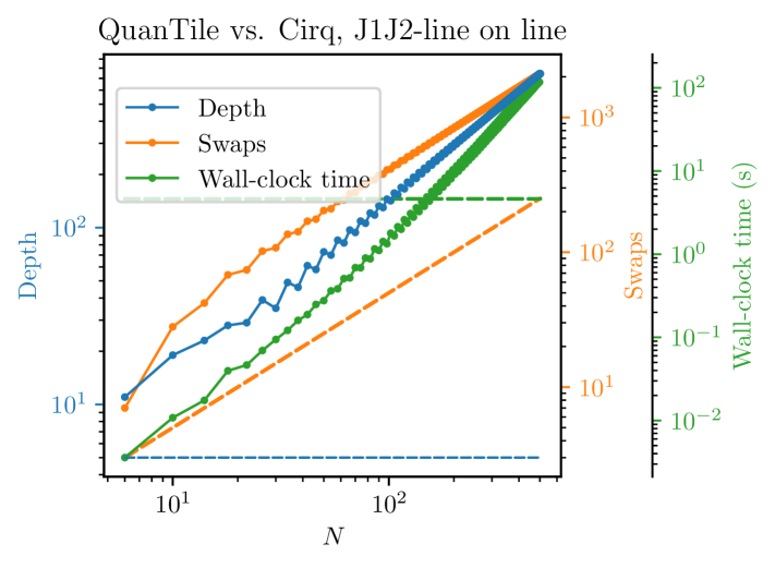
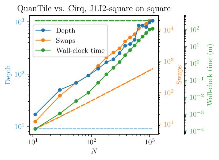
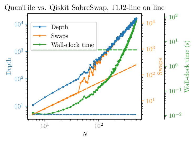
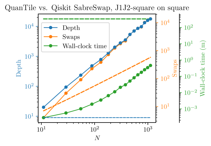
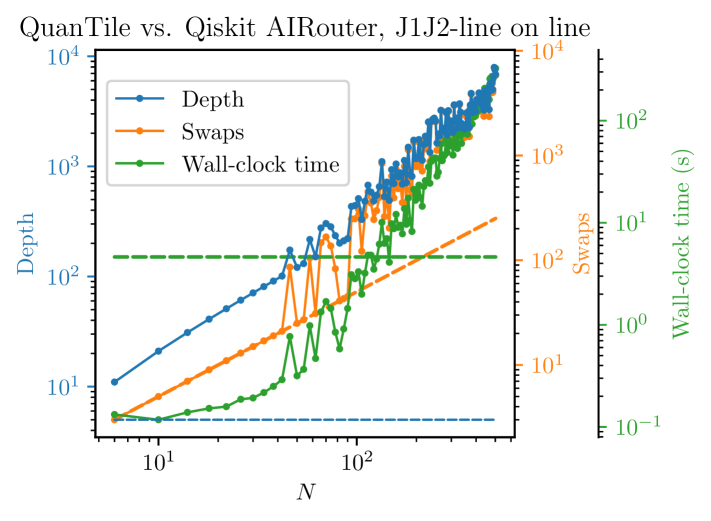
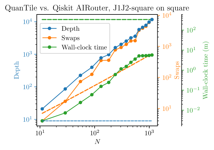
Figure 13: Benchmarking results of QuanTile against Cirq (first row), Qiskit SabreSwap (second row), and Qiskit AIRouter (third row) for routing a single Trotter step in the quantum simulation of a two-local Hamiltonian. The benchmarks are performed on two interaction graphs: a chain with nearest and next-nearest neighbor edges (J1J2-line, first column) and a square lattice with nearest and next-nearest neighbor edges (J1J2-square, second column). The horizontal axes show the system size $N$ – the number of qudits on which the Hamiltonian is defined.

VIII Basis graphs database

Here, we depict the basis graphs used in this work. They are defined in quantile/basis_graphs.json in the implementation [38]. Given an infinite lattice graph, the basis graph that induces it is not unique. So, for the circuits in Sec. VI to be fully unambiguous, it is necessary to give the basis graphs explicitly, which we do here. In Sec. VI, we used various basis graphs that generate the square lattice; they are all listed.

Each image depicts a patch of 5 by 5 basis graphs, with nodes represented using lattice graph notation. The central basis graph is highlighted with bold edges. Below each patch, the name of the corresponding basis graph is displayed. For the one-dimensional basis graphs, a patch of 5 by 1 basis graphs is shown.

We show the Archimedean lattices, the Laves lattices that are not also Archimedean, and miscellaneous other lattices. We gave a short introduction to these lattices in Ref. [33].

VIII.1 Archimedean

square

plus-square

diamond-square

honeycomb

triangular

square-octagon

trellis

snub-square

kagome

bridge

ruby

star

cross

VIII.2 Laves

union-jack

prismatic-pentagonal

cairo-pentagonal

dice

tetrille

asanoha

floret-pentagonal

kisrhombille

VIII.3 Miscellaneous

ladder

line

shuriken

J1J2-ladder

J1J2-line

J1J2-square

J1J2J3-square

heavy-hex