Supplementary Information

I Derivation of Hamiltonian

Nitrogen vacancy (NV) centers and substitutional nitrogen (P1) centers are the two primary spin defects in our diamond sample. The full Hamiltonian for all spins is given by

$$H =\sum_{j}\Delta s_{z,j}^{2}+\gamma_{\mathrm{NV}}\mathbf{s}_{j}\cdot\mathbf{B}+A_{z,j}s_{z,j}i_{z,j}+A_{\perp}(s_{x,j}i_{x,j}+s_{y,j}i_{y,j})$$ (1)

$$+\sum_{k}\gamma_{\mathrm{P1}}\mathbf{p}_{k}\cdot\mathbf{B}+H^{\mathrm{HF}}_{\mathrm{P1}}$$

$$+H_{\mathrm{NV-NV}}+H_{\mathrm{NV-P1}}+H_{\mathrm{P1-P1}}.$$

Here, $\mathbf{s}$ is the NV electronic spin-1 operator, $\mathbf{i}$ is the nuclear spin-1/2 operator for the ¹⁵N isotope, and $\mathbf{p}$ is the electronic spin-1/2 P1 operator. The gyromagnetic ratio of the electronic spin $\gamma_{\mathrm{NV}}\approx\gamma_{\mathrm{P1}}=(2\pi)\times 2.8~$MHz/G sets interactions with external magnetic fields $\mathbf{B}$, and the zero-field splitting is $\Delta=(2\pi)\times 2.87~$GHz. The electronic spin also interactions with the ¹⁵N nuclear spin via a hyperfine coupling with components $A_{z}=(2\pi)\times 3.03~$MHz and $A_{\perp}=(2\pi)\times 3.65~$MHz. The hyperfine interaction $H^{\mathrm{HF}}_{\mathrm{P1}}$ splits the P1 centers into four groups with different transition frequencies zuEmergentHydrodynamicsStrongly2021 . Finally, NV and P1 centers interact with each other $H_{\text{NV-NV}},~H_{\text{NV-P1}},~H_{\text{P1-P1}}$ via magnetic dipole-dipole interactions. We are primarily interested in $H_{\text{NV-NV}}$ and $H_{\text{NV-P1}}$, whose derivation follows.

I.1 NV-NV interaction $H_{\mathrm{NV-NV}}$

The native interaction between NV centers is the magnetic dipole-dipole interaction,

$$H_{\mathrm{NV-NV}}=-\sum_{i,j}\frac{J_{0}}{r_{ij}^{3}}[3(\mathbf{s}^{i}\cdot\hat{\mathbf{r}}_{ij})(\mathbf{s}^{j}\cdot\hat{\mathbf{r}}_{ij})-\mathbf{s}^{i}\cdot\mathbf{s}^{j}],$$ (2)

where $J_{0}=2\pi\times$52\text{\,}\mathrm{M}\mathrm{Hz}\cdot\mathrm{n}\mathrm{m}^{3}$$ is the interaction strength, $\hat{\mathbf{r}}_{ij}$ is the vector connecting spins $i$ and $j$. In the (111)-oriented diamond, we denote the out-of-the-plane direction as $\hat{\mathbf{z}}$. The vector $\hat{\mathbf{r}}_{ij}$ is perpendicular to $\hat{\mathbf{z}}$ and is parameterized by $(\cos\theta,\sin\theta,0)$, where $\theta$ is the azimuthal angle between two spins. For the NV group quantized along $\hat{\mathbf{z}}$, the dipolar interaction can then be explicitly written as

$$H_{\mathrm{NV-NV}} =-\sum_{i,j}\frac{J_{0}}{r_{ij}^{3}}[3(s^{i}_{x}\cos\theta+s^{i}_{y}\sin\theta)(s^{j}_{x}\cos\theta+s^{j}_{y}\sin\theta)-(s^{i}_{x}s^{j}_{x}+s^{i}_{y}s^{j}_{y}+s^{i}_{z}s^{j}_{z})]$$ (3)

$$=-\sum_{i,j}\frac{J}{r_{ij}^{3}}[(3\cos^{2}\theta-1)s^{i}_{x}s^{j}_{x}+(3\sin^{2}\theta-1)s^{i}_{y}s^{j}_{y}-s^{i}_{z}s^{j}_{z}+\cos\theta\sin\theta(s^{i}_{x}s^{j}_{y}+s^{i}_{y}s^{j}_{x})].$$

In the rotating frame, only the secular terms survive, i.e., $s^{i}_{x}s^{j}_{x}+s^{i}_{y}s^{j}_{y}$ (flip-flop) and $s^{i}_{z}s^{j}_{z}$ (Ising). We drop the non-secular flip-flip terms ($s^{i}_{x}s^{j}_{x}-s^{i}_{y}s^{j}_{y}$) and cross-terms $(s^{i}_{x}s^{j}_{y}+s^{i}_{y}s^{j}_{x})$. The dipolar Hamiltonian is reduced to the simple XXZ form for spin-1 operators

$$H_{\mathrm{NV-NV}}=-\sum_{i,j}\frac{J_{0}}{r_{ij}^{3}}[(s^{i}_{x}s^{j}_{x}+s^{i}_{y}s^{j}_{y})/2-s^{i}_{z}s^{j}_{z}].$$ (4)

In the experiment, we work in an effective two-level subspace $\{\ket{m_{s}=0},\ket{m_{s}=-1}\}$ of the full spin-1 ground state manifold. It is therefore convenient to further replace the spin-1 operators $\{s_{x},s_{y},s_{z}\}$ with spin-1/2 operators $\{\tilde{s}_{x},\tilde{s}_{y},\tilde{s}_{z}\}$, i.e.,

$$s_{x}\rightarrow\sqrt{2}\tilde{s}_{x},\ \ \ s_{y}\rightarrow\sqrt{2}\tilde{s}_{y},\ \ \ s_{z}\rightarrow\tilde{s}_{z}+\frac{I}{2}.$$ (5)

In this case, the dipolar Hamiltonian can be rewritten as

$$H_{\mathrm{NV-NV}}=-\sum_{i,j}\frac{J_{0}}{r_{ij}^{3}}[(\tilde{s}_{x}^{i}\tilde{s}_{x}^{j}+\tilde{s}_{y}^{i}\tilde{s}_{y}^{j})-\tilde{s}_{z}^{i}\tilde{s}_{z}^{j}-\tilde{s}_{z}^{i}-\tilde{s}_{z}^{j}].$$ (6)

The single-body terms $\tilde{s}_{z}$ can be treated as effective onsite disorder with characteristic strength $J_{0}$. Typically, the disorder emerging from the spin-1 to spin-1/2 reduction can be decoupled by e.g. XY-8 pulses, which are anyway needed to decouple the disorder arising from interactions with background spins $H_{\text{NV-P1}}$. Finally, we arrive at the effective XXZ Hamiltonian for NV-NV interaction in the spin-1/2 subspace:

$$H_{\mathrm{XXZ}}=-\sum_{i,j}\frac{J_{0}}{r_{ij}^{3}}[(\tilde{s}_{x}^{i}\tilde{s}_{x}^{j}+\tilde{s}_{y}^{i}\tilde{s}_{y}^{j})-\tilde{s}_{z}^{i}\tilde{s}_{z}^{j}].$$ (7)

From now on, we drop the tilde on the effective spin-1/2 operator for simplicity.

I.2 NV-P1 interaction $H_{\mathrm{NV-P1}}$

NV and P1 centers similarly interact through the magnetic dipole-dipole interaction,

$$H_{\mathrm{NV-P1}}=-\sum_{i,j}\frac{J_{0}}{r_{ij}^{3}}[3(\mathbf{s}^{i}\cdot\hat{\mathbf{r}}_{ij})(\mathbf{p}^{j}\cdot\hat{\mathbf{r}}_{ij})-\mathbf{s}^{i}\cdot\mathbf{p}^{j}].$$ (8)

Because of the zero-field splitting $\Delta$ of the NV center, spin-exchange interactions between NV and P1 centers are highly off-resonant and naturally drop out in the rotating frame. The only surviving term is the Ising coupling that conserves the total energy, i.e.,

$$H_{\mathrm{NV-P1}}=\sum_{i,j}\frac{J_{0}}{r_{ij}^{3}}s^{i}_{z}p^{j}_{z}.$$ (9)

In the experiment, we employ an XY-8 pulse sequence to decouple these Ising interactions. With NV centers mostly polarized in the $m_{I}=-1/2$ nuclear spin subgroup [Methods, Sec. I.3], the only relevant term in Eq. 1 is $H_{\mathrm{XXZ}}$.

II Numerical simulations

II.1 Numerical methods

To simulate the dynamics of the disordered, interacting NV centers, we use the discrete cluster TWA and neural quantum state (NQS) numerical methods, which are benchmarked against Krylov subspace methods for small system sizes.

II.1.1 Krylov subspace method

The Krylov method solves the Schrödinger equation in a so-called Krylov subspace with reduced dimensionality Krylov . Instead of directly diagonalizing the full Hamiltonian, the method constructs a series of smaller, more manageable Krylov subspaces. These subspaces are generated by repeatedly applying the Hamiltonian to an initial state vector, effectively capturing the most significant components of the system dynamics within a reduced basis. By projecting the Hamiltonian onto this Krylov subspace, one can compute approximate eigenvalues and eigenvectors, enabling the efficient calculation of the time evolution operator. This approach allows for the efficient simulation of quantum dynamics for systems that are otherwise too large for traditional exact diagonalization methods. In our work, we employ the Krylov subspace method using the Dynamite package meyerKrylov2024 to simulate dynamics of the NV spins. Although this method can compute the exact time evolution of the spins, it is limited to relatively small system sizes $N\leq 30$ due to memory limitations ($\sim$ 2000 GB per cluster node).

In this work, we primarily perform Krylov on a $N=20$ random spin ensemble, balancing the computational cost (runtime and memory usage) with the ability to capture the essential features of the system’s time evolution. For simulations on the systems with positional disorder, we randomly sample the spatial disorder realizations and execute the calculations in parallel on the computing cluster.

II.1.2 discrete Wigner function approximation methods

The discrete truncated Wigner approximation (DTWA) schachenmayerManyBodyQuantumSpin2015 is a method that approximately simulates quantum dynamics using an ensemble of classical Monte Carlo trajectories. In this approach, each trajectory involves the evolution of classical spins under the same Hamiltonian, with initial states randomly sampled from a discrete Wigner distribution corresponding to the initial quantum state. This numerical method captures the time evolution of one- and two-point correlators at the mean-field level, which is crucial for simulating the squeezing dynamics. Compared to the Krylov method, DTWA can access much larger system sizes, e.g., up to $N\sim 10^{5}$ blockScalableSpinSqueezing2024 . However, the original method is insufficient for quantitatively studying the dynamics of disordered spin systems because it captures quantum correlations only at the mean-field level. Consequently, it fails to accurately simulate the fast dynamics between closely spaced, strongly interacting spin pairs, i.e., dimers.

To overcome this limitation, we apply a cluster generalization of the original method alaouiMeasuringBipartiteSpin2024 ; braemerClusterTruncatedWigner2024 ; nagaoTwodimensionalCorrelationPropagation2024 , known as discrete cluster truncated Wigner approximation (cluster DTWA). In this method, spins within a dimer are grouped into a cluster, and the full quantum degrees of freedom of the cluster are represented using a classical vector whose state space dimension accounts for the combined Hilbert space of the spins in the cluster. For a dimer consisting of two spin-$1/2$ particles, this corresponds to a four-dimensional Hilbert space with 15 independent operators, reflecting the generators of the SU(4) Lie algebra. Similar to the original method, the cluster method utilizes classical Monte Carlo trajectories, but it treats the interactions within each cluster exactly in a quantum mechanical way, while employing a mean-field approximation for the interactions between clusters. The cluster method provides a much better description of the fast dynamics within dimers and is, in general, a more accurate numerical method for disordered systems compared to the original method. Note that the performance of the cluster method depends on how clusters are chosen: the numerical result is the most accurate when the most strongly interacting spins are clustered together. Here, we apply the real space renormalization group (RSRG) inspired method proposed in braemerClusterTruncatedWigner2024 , which clusters the spins based on pairwise interaction strength.

II.1.3 Neural quantum states

We also utilize neural quantum states (NQS) carleoSolvingQuantumManybody2017 to simulate the dynamics. This method employs neural networks to represent and study quantum many-body systems within the framework of the time-dependent variational principle (TDVP) haegeman2011time . Coefficients $\psi_{s}$ in the computational basis of the quantum state $|\psi\rangle=\sum_{s}\psi_{s}|s\rangle$ are parametrized by a neural network $\psi_{\theta}:s\mapsto\psi_{\theta}(s)$. By leveraging the TDVP, the parameters of the neural network are dynamically updated to approximate the solution of the Schrödinger equation over time carleoSolvingQuantumManybody2017 . Given a neural network state $|\psi(\theta)\rangle$ at time $t$ , we update its parameters for time $t+\delta t$ by applying a first-order expansion of the propagator and then projecting the resulting state back onto the neural network’s parameter manifold [Fig. 1b]. This approach leads to an ODE of the form $S\dot{\theta}=-iF$ , where $F=-\nabla_{\theta}\langle H\rangle$ is the gradient vector and $S$ is the quantum Fisher matrix schmitt2020quantum ; carleoSolvingQuantumManybody2017 . Both $F$ and $S$ are estimated using Monte Carlo Markov Chain techniques. To find the updated neural network state $|\psi(\theta+\delta\theta^{*})\rangle$ at time $t+\delta t$ , we solve the ODE for $\theta(t)$ using numerical integration methods such as Euler or Runge-Kutta. This framework enables simulation of real-time dynamics, including the system’s response to quenches and time-dependent perturbations.

We believe that NQS has several strengths that complement other numerical approaches mentioned above. On the one hand, as compared with (essentially) exact Krylov methods, NQS can scale to much larger system sizes. On the other hand, in contrast to semiclassical DTWA methods, NQS enables a much better controlled approximation, allowing it to more accurately capture the evolution of quantum correlations schmitt2020quantum ; schmitt2022quantum ; sinibaldi2023unbiasing . The degree of approximation within NQS is mainly set by neural network hyperparameters, size of the integration timestep, and number of samples used for evaluating equations of motion for neural network parameters. Furthermore, in the ideal limit, NQS dynamics preserves conserved quantities haegeman2011time , providing an intrinsic benchmark for checking numerical stability when comparing to an exact solution is not possible.

To arrive at optimal NQS parameters, we have conducted ablation studies. For our simulations, we use the restricted Boltzmann machine (RBM) architecture [Fig. 1a] with complex parameters and tunable hidden layer density $\alpha_{\text{RBM}}$ ranging from $0.75$ to $4$. We choose a 4th-order Runge-Kutta method with $\delta t=5\cdot 10^{-3}$ for the numerical integration of the TDVP equations. We ran all simulations with $N_{\mathrm{samples}}=2^{16}$ run on $2^{10}$ Monte Carlo Markov chains and a quantum Fisher matrix regularization of $\epsilon_{\text{RBM}}=10^{-4}$. To ensure efficient parallelization and runtime, our simulations were run on NVIDIA A100 and H100 GPUs with NetKet vicentini2022netket and JAX jax2018github .

II.2 Benchmark between numerical methods

We carefully benchmark the different numerical algorithms. Starting with a small system size $N=20$, cluster DTWA and NQS are benchmarked by the Krylov subspace method, which is known to be relatively accurate. As shown in Fig. 1(d-e), all of the three numerical methods exhibit quantitative agreement among the collective spin length, minimal variance and the squeezing parameter, indicating that both cluster DTWA and NQS capture the system dynamics to a high accuracy.

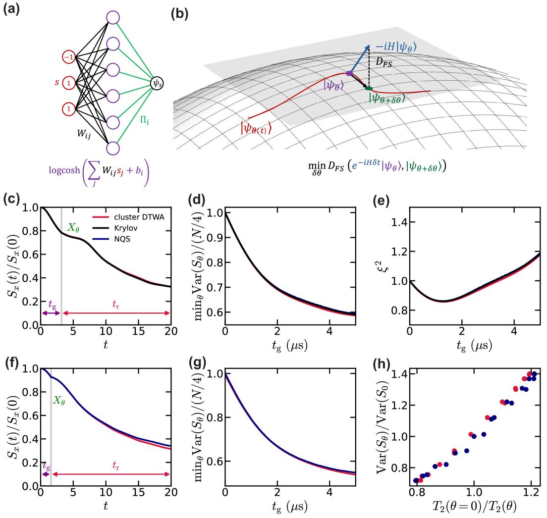
Figure 1: Numerical benchmark between cluster DTWA, NQS and Krylov subspace method. (a) Restricted Boltzmann machine neural network architecture used for NQS simulations. (b) NQS enables the simulation of time dynamics within the TDVP framework by identifying the nearest quantum state on the NQS manifold to the Hamiltonian-evolved state, using the Fubini-Study metric $D_{FS}$ carleoSolvingQuantumManybody2017 . When expanded to first-order in $\mathcal{O(\delta\theta)}$ and $\mathcal{O}(\delta t)$, this approach results in an ODE governing the parameter evolution. (c, d, e) Numerical simulation of a small $N=20$ system with reduced disorder $r_{\mathrm{shelve}}=7$ nmn and perfect initial state polarization. We simulate the $S_{x}(t)$ decay profile in the generation quench (up to $t_{\mathrm{g}}=3.2\ \mu\mathrm{s}$) and the readout quench (up to $t_{\mathrm{r}}=16.8\ \mu\mathrm{s}$) in (a). We apply a $X_{\theta}$ rotation ($\theta=\pi/4$) between the generation and detection quench to align certain collective spin operator $S_{\theta}$ into $S_{z}$. We simulate the time evolution of the minimal variance and squeezing parameter up to $t_{\mathrm{g}}=5\ \mu\mathrm{s}$ in (d) and (e), respectively. (f, g, h) Numerical simulation of a $N=80$ system with reduced disorder $r_{\mathrm{shelve}}=7$ nm and perfect initial state polarization. We simulate the $S_{x}(t)$ decay profile in the generation quench (up to $t_{\mathrm{g}}=1.6\ \mu\mathrm{s}$) and the readout quench (up to $t_{\mathrm{r}}=18.4\ \mu\mathrm{s}$) in (a). We simulate the time evolution of the minimal variance in (g). Based on the $S_{x}(t_{\mathrm{r}})$ decay profile in the readout quench, we shows the mapping extracted in (g) following the procedure detailed in the Method.

To further benchmark the performance of cluster DTWA compared to NQS, we enlarge our system size to $N=80$, which is used extensively in all other numerical simulations in this work. Fig. 1(f-g), again, shows a quantitative agreement between cluster DTWA and NQS for both the collective spin length and the minimal variance. Based on the numerical simulation of the readout quench profile $S_{x}(t_{\mathrm{r}})$ in Fig. 1f, we extract the mapping between the $T_{2}$ decay timescale and the variance $\mathrm{Var}(S_{\theta})$ with both numerical methods [Fig. 1h], which shows a reasonably good agreement. By benchmarking cluster DTWA and NQS at a system size beyond the computational ability of any exact numerical methods and reaching a high consistency, we conclude that both cluster DTWA and NQS accurately simulate the time evolution for a positionally disordered system under $H_{\mathrm{XXZ}}$.

III Probing quantum variance via quench dynamics

In this section, we present details of the experimental protocol that probes the variance of the quantum spin projection noise by measuring the timescale of the quench dynamics under the $H_{\mathrm{XXZ}}$ after the preparation of a spin-squeezed state. The essence of this protocol is a relation between the twisting speed, which is proportional to the quantum variance, and the $S_{x}$ decay timescale.

III.1 Dynamics under OAT Hamiltonian

We first present an analytical derivation of the $S_{x}(t_{\mathrm{r}})$ decay profile for the quench under $H_{\mathrm{OAT}}$. We start with a Gaussian initial state along $+x$ axis ($\expectationvalue{S_{x}}>0$, $\expectationvalue{S_{y}}=\expectationvalue{S_{z}}=0$), and its Wigner function is a Gaussian distribution,

$$P(S_{y},S_{z})=\frac{1}{2\pi\sigma_{Y}\sigma_{Z}\sqrt{1-\rho^{2}}}\exp(-\frac{1}{2(1-\rho^{2})}\quantity[\frac{S_{y}^{2}}{\sigma_{Y}^{2}}+\frac{S_{z}^{2}}{\sigma_{Z}^{2}}-2\rho\frac{S_{y}S_{z}}{\sigma_{Y}\sigma_{Z}}]),$$ (10)

where we slightly abuse the notation by denoting $S_{\mu}$ as both the quantum spin operator and the classical variable associated with the spin operator. The quantum noise is captured by $\mathrm{Var}(S_{y})=\sigma_{Y}^{2}$, $\mathrm{Var}(S_{z})=\sigma_{Z}^{2}$ and $\expectationvalue{S_{y}S_{z}}=\rho\sigma_{Y}\sigma_{Z}$. Under $H_{\mathrm{OAT}}=\chi S_{z}^{2}$, the time evolution of the Wigner quasiprobability distribution is the precession about the $z$-axis with a rate proportional to $Z$, i.e.,

$$\expectationvalue{S_{x}(t_{\mathrm{r}})|S_{z}} =L\cos(\phi_{0}S_{z}+2S_{z}\chi t_{\mathrm{r}})$$ (11)

$$\expectationvalue{S_{y}(t_{\mathrm{r}})|S_{z}} =L\sin(\phi_{0}S_{z}+2S_{z}\chi t_{\mathrm{r}}),$$

where $L=\sqrt{\expectationvalue{S_{x}^{2}+S_{y}^{2}}}$ is the effective spin length, and $t_{\mathrm{r}}$ is the evolution time. $\phi_{0}$ is specified by the initial condition

$$L\sin(\phi_{0}S_{z})=\expectationvalue{S_{y}(t_{\mathrm{r}}=0)|S_{z}}=\rho\frac{\sigma_{Y}}{\sigma_{Z}}S_{z}=\frac{\expectationvalue{S_{y}S_{z}}}{\sigma_{Z}^{2}}S_{z},$$ (12)

where $\expectationvalue{S_{y}(t_{\mathrm{r}}=0)|S_{z}}=\rho\frac{\sigma_{Y}}{\sigma_{Z}}S_{z}$ is a direct consequence of Eq. (10).

When $\phi_{0}$ is small, we have $\phi_{0}=\frac{\expectationvalue{S_{y}S_{z}}}{\sigma_{Z}^{2}L}$. Therefore,

$$\expectationvalue{S_{x}(t_{\mathrm{r}})} =\int\expectationvalue{S_{x}(t_{\mathrm{r}})|S_{z}}P(S_{z})\differential{S_{z}}=L\int\cos(\quantity[\frac{\expectationvalue{S_{y}S_{z}}}{\sigma_{Z}^{2}L}+2\chi t_{\mathrm{r}}]S_{z})P(S_{z})\differential{S_{z}}$$ (13)

$$=L\exp(-\frac{1}{2}\sigma_{Z}^{2}\quantity(\frac{\expectationvalue{S_{y}S_{z}}}{\sigma_{Z}^{2}L}+2\chi t_{\mathrm{r}})^{2})=L\exp(-2\chi^{2}\mathrm{Var}(S_{z})(t_{\mathrm{r}}-t_{\mathrm{o}})^{2})$$

$$=L\exp(-\quantity(\frac{t_{\mathrm{r}}-t_{\mathrm{o}}}{T_{2}})^{2}),$$

where we use $P(S_{z})=\frac{1}{\sqrt{2\pi}\sigma_{Z}}e^{-\frac{S_{z}^{2}}{2\sigma_{Z}^{2}}}$. Here, $T_{2}$ is the characteristic decay timescale and $t_{\mathrm{o}}$ is an offset time, i.e.,

$$T_{2}=\frac{1}{\sqrt{2}\chi\sqrt{\mathrm{Var}(S_{z})}},\ \ \ t_{\mathrm{o}}=-\frac{\expectationvalue{S_{y}S_{z}}}{2\chi\mathrm{Var}(S_{z})L}.$$ (14)

Note that the offset time $t_{\mathrm{o}}$ can be either positive and negative, depending on the sign of the correlator $\expectationvalue{S_{y}S_{z}}$.

Crucially, $T_{2}$ has a one-to-one correspondence to the quantum variance $\mathrm{Var}(S_{z})=\sigma_{Z}$, which exactly reflects the fact that the quantum state with a larger $\mathrm{Var}(S_{z})$ twists and wraps along the Bloch sphere faster. This correspondence enables us to extract the quantum variance by only measuring the collective observable $S_{x}$, which no longer requires the quantum-projection-noise-limited state readout. Furthermore, $t_{\mathrm{o}}$ is time when $S_{x}(t)$ reaches its maximum, i.e., $\max_{t}S_{x}(t)=S_{x}(t_{\mathrm{o}})$, where the quantum state is minimally wrapped around the Bloch sphere. Note that

$$\expectationvalue{S_{y}S_{z}(t)}=\int\expectationvalue{S_{x}(t_{\mathrm{r}})|S_{z}}S_{z}P(S_{z})\differential{S_{z}}=L\sigma_{z}^{2}\exp(-\frac{1}{2}\sigma_{z}^{2}\quantity(2\frac{\chi}{N}t+\phi_{0})^{2})\quantity(2\frac{\chi}{N}t+\phi_{0}).$$ (15)

Therefore, we have $\expectationvalue{S_{y}S_{z}(t_{\mathrm{o}})}=0$, indicating that the squeezing direction of the state is either along $y$ or $z$ direction at $t=t_{\mathrm{o}}$, which further justify that the quantum state at $t=t_{\mathrm{o}}$ is minimally wrapped around the Bloch sphere. Here, a positive (negative) $t_{\mathrm{o}}$ means that one has to perform forward (backward) time evolution to unwrapped the initial state.

Practically, to extract the decay time $T_{2}$ from the $S_{x}(t)$ decay profile, we first redefine the effective readout time $t_{\mathrm{r}}^{\mathrm{eff}}=t_{\mathrm{r}}-t_{\mathrm{o}}$, where $t_{\mathrm{r}}^{\mathrm{eff}}=0$ corresponds to the minimally-wrapped state. Then, we extract the decay timescale by fitting the decay profile with a stretched exponential functional form, i.e, $S_{x}(t_{\mathrm{r}}^{\mathrm{eff}})\sim\exp(-(t_{\mathrm{r}}^{\mathrm{eff}}/T_{2})^{\alpha})$, where $\alpha=2$ for the OAT case. This protocol can be alternatively understood as follows:

1. For an initial state with $\expectationvalue{S_{y}S_{z}}=0$, $S_{x}(t_{\mathrm{r}})$ has a monotonic decay profile, where one can directly extract a timescale $T_{2}$ by fitting the decay profile to a stretched exponential functional form without any offset time $t_{\mathrm{o}}$.

2. For an initial state with $\expectationvalue{S_{y}S_{z}}\neq 0$, one can forward (backward) evolution the quantum state by a time $t=-t_{\mathrm{o}}$ to prepare an intermediate state with $\expectationvalue{S_{y}S_{z}}=0$. Then, one measure thes quench dynamics for the intermediate step and follow the step 1 to extract a decay timescale $T_{2}$, which corresponds to $\mathrm{Var}(S_{z})$ of the intermediate state. Use the fact that time evolution under $H_{\mathrm{OAT}}$ preserve $S_{z}$, the initial state ($\expectationvalue{S_{y}S_{z}}\neq 0$) and the intermediate state ($\expectationvalue{S_{y}S_{z}}=0$) has the same $\mathrm{Var}(S_{z})$. Therefore, the one-to-one correspondence between $T_{2}$ and $\mathrm{Var}(S_{z})$ for the intermediate state can be directly applied to the initial state, i.e., the measured timescale $T_{2}$ can be directly used to infer $\mathrm{Var}(S_{z})$ for the initial state.

The second case above is exactly the same as redefining the effective readout time, since the preparation of the intermediate state and the quench measurement of the intermediate are all just the quench from the initial state. In practice, one can extract $t_{\mathrm{o}}$ from the effective twisting strength (Sec. III.2). Beyond $H_{\mathrm{OAT}}$, the aforementioned protocols also works for $H_{\mathrm{XXZ}}$ in our experiment, where the same derivation can be performed with an early-time expansion as sketched in the next section.

III.2 Dynamics under XXZ Hamiltonian

After establishing the protocol under the $H_{\mathrm{OAT}}$, we now show that the sample procedure also applies to the disorder XXZ Hamiltonian $H_{\mathrm{XXZ}}$. We perform an early time expansion in the Heisenberg picture to analyze the time evolution of the collective spin operators.

The time evolution of an operator $O$ is given by

$$O(t)=O+it[H,O]+\frac{1}{2}(it)^{2}[H,[H,O]]+\mathcal{O}(t^{3}).$$ (16)

For the dipolar interacted system, the Hamiltonian can be separated into Heisenberg part and Ising part, i.e.,

$$H=-J\sum_{i,j}\frac{1}{r_{ij}^{3}}[(s_{x}^{i}s_{x}^{j}+s_{y}^{i}s_{y}^{j}+s_{z}^{i}s_{z}^{j})-2s_{z}^{i}s_{z}^{j}]=H_{\mathrm{Hei}}+H_{\mathrm{Ising}}.$$ (17)

Because the initial coherent spin state is the eigenstate of the Heisenberg Hamiltonian $H_{\mathrm{Hei}}$, we expect that $\expectationvalue{[H_{\mathrm{Hei}},O]}\simeq 0$ in the early time, where $O$ can be any (single or multiple body) operator. Therefore, we have

$$\expectationvalue{[H,O]}=\expectationvalue{[H_{\mathrm{Hei}},O]}+\expectationvalue{[H_{\mathrm{Ising}},O]}=\expectationvalue{[H_{\mathrm{Ising}},O]}$$ (18)

Denote $J^{\prime}=-2J$ in the following derivation. We have

$$\ [H_{\mathrm{Ising}},S_{x}] =J^{\prime}\sum_{ij}\frac{1}{r_{ij}^{3}}\sum_{m}[s_{z}^{i}s_{z}^{j},s_{x}^{m}]=J^{\prime}\sum_{i<j,m}\frac{1}{r_{ij}^{3}}i[\delta_{im}s_{y}^{i}s_{z}^{j}+\delta_{jm}s_{z}^{i}s_{y}^{j}]=J^{\prime}\sum_{i<j}\frac{1}{r_{ij}^{3}}i[s_{y}^{i}s_{z}^{j}+s_{z}^{i}s_{y}^{j}]$$ (19)

$$[H_{\mathrm{Ising}},S_{y}] =J^{\prime}\sum_{ij}\frac{1}{r_{ij}^{3}}\sum_{m}[s_{z}^{i}s_{z}^{j},s_{y}^{m}]=J^{\prime}\sum_{i<j,m}\frac{1}{r_{ij}^{3}}(-i)[\delta_{im}s_{x}^{i}s_{z}^{j}+\delta_{jm}s_{z}^{i}s_{x}^{j}]=J^{\prime}\sum_{i<j}\frac{1}{r_{ij}^{3}}(-i)[s_{x}^{i}s_{z}^{j}+s_{z}^{i}s_{x}^{j}]$$

$$\ [H_{\mathrm{Ising}},[H_{\mathrm{Ising}},S_{x}]] =J^{\prime 2}\sum_{i<j;m<n}\frac{i}{r_{ij}^{3}r_{mn}^{3}}[s_{z}^{i}s_{z}^{j},s_{y}^{m}s_{z}^{n}+s_{z}^{m}s_{y}^{n}]$$ (20)

$$=J^{\prime 2}\sum_{i<j;m<n}\frac{i}{r_{ij}^{3}r_{mn}^{3}}([s_{z}^{i}s_{z}^{j},s_{y}^{m}]s_{z}^{n}+s_{z}^{m}[s_{z}^{i}s_{z}^{j},s_{y}^{n}])$$

$$=J^{\prime 2}\sum_{i<j;m<n}\frac{1}{r_{ij}^{3}r_{mn}^{3}}(\delta_{im}s_{x}^{i}s_{z}^{j}s_{z}^{n}+\delta_{jm}s_{z}^{i}s_{x}^{j}s_{z}^{n}+\delta_{in}s_{z}^{m}s_{x}^{i}s_{z}^{j}+\delta_{jn}s_{z}^{m}s_{z}^{i}s_{x}^{j})$$

Here, we would like to derive Eq.(11) for $H_{\mathrm{XXZ}}$, which requires the calculation of the expectation value of collective spin operators for an initial spin coherent states offsetted from the $+x$ axis by an angle $\theta$ such that $\expectationvalue{S_{z}}=N\sin\theta/2$. Rather than rotate the quantum state, we can rotate the reference frame by an angle of $\theta$ (redefining $s_{\mu}^{i}$ operators) such that the offset state becomes $\ket{+x}$ in the new frame. In the leading order, we get

$$\expectationvalue{[H_{\mathrm{Ising}},S_{x}]} =0$$ (21)

$$\expectationvalue{[H_{\mathrm{Ising}},S_{y}]} =J^{\prime}\sum_{i<j}\frac{1}{r_{ij}^{3}}(-i)2\sin\theta\cos\theta=-2i\sin\theta\cos\theta J_{\mathrm{eff}},$$

where $J_{\mathrm{eff}}=J^{\prime}\sum_{i<j}1/r_{ij}^{3}$. Therefore, the semiclassical evolution of the collective spin operator is

$$\expectationvalue{S_{x}(t)|S_{z}} =S_{x}(0)|S_{z}+it\expectationvalue{[H,S_{x}]}+\mathcal{O}(t^{2})=\frac{N}{2}+\mathcal{O}(t^{2}),$$ (22)

$$\expectationvalue{S_{y}(t)|S_{z}} =S_{y}(0)|S_{z}+it\expectationvalue{[H,S_{y}]}+\mathcal{O}(t^{2})=2\sin\theta\cos\theta J_{\mathrm{eff}}t+\mathcal{O}(t^{2})\simeq\frac{4S_{z}}{N}J_{\mathrm{eff}}t+\mathcal{O}(t^{2}),$$

where we have used $S_{z}=\frac{N}{2}\sin\theta$ and assumed $\cos\theta\simeq 1$ for small $\theta$. Note that this equation is in the same form as Eq.(11). In the semiclassical picture, the initial coherent spin state is approximated by a Gaussian distribution $P(S_{z})=\sqrt{\frac{2}{\pi\eta N}}\exp(-\frac{2S_{z}^{2}}{\eta N})$, where $\mathrm{Var}(S_{z})=\expectationvalue{S_{z}^{2}}=\eta N/4$. Therefore,

$$\expectationvalue{S_{x}(t)} =\int\expectationvalue{S_{x}(t)|S_{z}}P(S_{z})\differential{S_{z}}$$ (23)

$$\expectationvalue{S_{y}S_{z}(t)} =\int\expectationvalue{S_{y}(t)|S_{z}}S_{z}P(S_{z})\differential{S_{z}}=\int\quantity(\frac{4S_{z}}{N}J_{\mathrm{eff}}t)S_{z}P(S_{z})\differential{S_{z}}=\eta J_{\mathrm{eff}}t,$$

$$\expectationvalue{S_{y}^{2}(t)} =\mathrm{Var}(S_{y}|S_{z})+\int\expectationvalue{S_{y}(t)|S_{z}}^{2}P(S_{z})\differential{S_{z}}=\frac{N}{4\eta}+\frac{4\eta J_{\mathrm{eff}}^{2}t^{2}}{N}$$

As a result, we have

$$\frac{\expectationvalue{S_{y}S_{z}(t)}}{\expectationvalue{S_{z}^{2}}} =\frac{4J_{\mathrm{eff}}t}{N}=\chi t,$$ (24)

$$\frac{\expectationvalue{S_{y}^{2}(t)}}{\expectationvalue{S_{z}^{2}}} =\frac{1}{\eta^{2}}+\frac{16J_{\mathrm{eff}}^{2}t^{2}}{N^{2}}=\frac{1}{\eta^{2}}+(\chi t)^{2},$$

where we denote $\chi=4J_{\mathrm{eff}}/N$.

Now, given that we have prepared a squeezing state by the time evolution under $H_{\mathrm{XXZ}}$, in order to measure $\mathrm{Var}(S_{\theta})$, we apply a global rotation $\theta$ along the $x$ axis. The correlators for the state after rotation is

$$\expectationvalue{S_{y}S_{z}(\theta)} =(\cos^{2}\theta-\sin^{2}\theta)\expectationvalue{S_{y}S_{z}}+\sin\theta\cos\theta(\expectationvalue{S_{y}^{2}}-\expectationvalue{S_{z}^{2}})$$ (25)

$$\expectationvalue{S_{z}^{2}(\theta)} =\cos^{2}\theta\expectationvalue{S_{z}^{2}}+\sin^{2}\theta\expectationvalue{S_{y}^{2}}+2\sin\theta\cos\theta\expectationvalue{S_{y}S_{z}},$$

where $\expectationvalue{S_{y}^{2}}$, $\expectationvalue{S_{z}^{2}}$ and $\expectationvalue{S_{y}S_{z}}$ denote the correlators for the state before the $\theta$ rotation, which satisfy Eq.(24).

Note that the offset time $t_{\mathrm{o}}$ is defined as the time such that $\expectationvalue{S_{y}S_{z}(t_{\mathrm{o}})}=0$, i.e., the squeezing direction is either along the $+y$ or $+z$ direction. From Eq. (24), we have

$$\chi t_{\mathrm{o}} =-\frac{\expectationvalue{S_{y}S_{z}(\theta)}}{\expectationvalue{S_{z}^{2}(\theta)}}$$ (26)

$$=-\frac{(\cos^{2}\theta-\sin^{2}\theta)\expectationvalue{S_{y}S_{z}}+\sin\theta\cos\theta(\expectationvalue{S_{y}^{2}}-\expectationvalue{S_{z}^{2}})}{\cos^{2}\theta\expectationvalue{Z^{2}}+\sin^{2}\theta\expectationvalue{S_{y}^{2}}+2\sin\theta\cos\theta\expectationvalue{S_{y}S_{z}}}$$

$$=-\frac{(1-\tan^{2}\theta)\frac{\expectationvalue{S_{y}S_{z}}}{\expectationvalue{S_{z}^{2}}}+\tan\theta\quantity(\frac{\expectationvalue{S_{y}^{2}}}{\expectationvalue{S_{z}^{2}}}-1)}{1+\tan^{2}\theta\frac{\expectationvalue{S_{y}^{2}}}{\expectationvalue{S_{z}^{2}}}+2\tan\theta\frac{\expectationvalue{S_{y}S_{z}}}{\expectationvalue{S_{z}^{2}}}}$$

Now, we can apply Eq. (24) again to replace the correlators $\expectationvalue{S_{y}^{2}}$, $\expectationvalue{S_{z}^{2}}$ and $\expectationvalue{S_{y}S_{z}}$ by the preparation time,

$$\chi t_{\mathrm{o}} =-\frac{(1-\tan^{2}\theta)\chi t_{\mathrm{g}}+\tan\theta(\chi t_{\mathrm{g}})^{2}}{1+\tan^{2}\theta(1+(\chi t_{\mathrm{g}})^{2})+2\tan\theta\chi t_{\mathrm{g}}}.$$ (27)

This is the analytical formula to extract the offset time $t_{\mathrm{o}}$.

We note that the asymptotic behavior in the $\chi t_{\mathrm{g}}\rightarrow 0$ limit is

$$\lim_{\chi t_{\mathrm{g}}\rightarrow 0}\frac{\chi t_{\mathrm{o}}}{\chi t_{\mathrm{g}}} =-\frac{1-\tan^{2}\theta}{1+\tan^{2}\theta}=-\cos(2\theta),$$ (28)

which can be used as a rough estimation if $\chi$ is unknown. However, in reality, the effective mean field interaction strength $\chi$ can be characterized by the average twisting experiment, where the initial coherent spin state is rotated along the $y$ axis by an angle $\theta$ such that $Z=\frac{N}{2}\sin\theta$. Eq.(22) provides a description for dynamics of the average motion of the coherent spin state, i.e.,

$$\frac{S_{y}(t)}{S_{x}(t)}=\chi t\sin\theta,$$ (29)

where $S_{y}(t)$ and $S_{x}(t)$ are measured in the average twisting experiment. Therefore, we finally get

$$\chi=\frac{1}{\sin\theta}\lim_{t\rightarrow 0}\quantity(\frac{S_{y}(t)/S_{x}(t)}{t}),$$ (30)

where we take the early time limit $t\rightarrow 0$. This equation is used to extract the interaction strength $\chi$ for the average spin twisting measurement.

IV Effect of dimers in the disordered system

In the system with positional disorder, as discussed in the main text, the existence of strongly-interacting NV dimers causes a rapid decay of the collective spin length which prohibits spin squeezing. In this section, we provide a more thorough discussion of the effect of the dimers on the mean-field twisting and variance readout measurements.

IV.1 Stretch power as a measure of lattice geometry

The dynamics of the spin-polarized state $\ket{\mathbf{x}}$ under $H_{\mathrm{XXZ}}$ exhibit a single stretched exponential decay $S_{x}(t)\sim e^{-(t/\tau)^{p}}$. As described in the main text, the stretch power $p$ indicates the spatial geometry of the spin ensemble. Here, we provide an analytical derivation showing the crossover from the early-time Gaussian dynamics $p=2$ to late-time disordered dynamics $p=2/3$ in the lattice-engineered system, as discussed in Sec. III.1 of the Methods.

In the early time regime, the Hamiltonian can be separated into Heisenberg and Ising parts as

$$H_{\mathrm{XXZ}}=H_{\mathrm{Hei}}+H_{\mathrm{Ising}}=-J_{0}\sum_{i,j}\frac{1}{r_{ij}^{3}}(s_{x}^{i}s_{x}^{j}+s_{y}^{i}s_{y}^{j}+s_{z}^{i}s_{z}^{j})+2J_{0}\sum_{i,j}\frac{1}{r_{ij}^{3}}s_{z}^{i}s_{z}^{j};$$ (31)

we hereafter set the interaction strength $J_{0}=1$ throughout this section for simplicity. Because $H_{\mathrm{Hei}}$ commutes with $S_{x}$, the quench dynamics $S_{x}(t)$ are dominated by the Ising interaction. Therefore, the quench profile $S_{x}(t)$ can be derived analytically following Eq.(S9) in Ref. davisProbingManybodyDynamics2023 , i.e.,

$$S_{x}(t) =\exp{-n\int_{r_{\mathrm{min}}}^{\infty}\differential{r}r\int\differential{\Omega}\quantity(1-e^{-\frac{\chi(t)}{8r^{6}}})}$$ (32)

$$=\exp{-2\pi n\int_{r_{\mathrm{min}}}^{\infty}\differential{r}r\quantity(1-e^{-\frac{\chi(t)}{8r^{6}}})}$$

$$=\exp{-2\pi n\quantity[\frac{r_{\mathrm{min}}^{2}}{6}\quantity(\mathrm{E}_{4/3}\quantity(\frac{\chi(t)}{8r_{\mathrm{min}}^{6}})-3)-\frac{\chi(t)^{1/3}}{12}\Gamma\quantity(-\frac{1}{3})]}.$$

Here, $n$ is the spin density, $E_{m}(x)=\int_{1}^{\infty}e^{-xt}/t^{m}\differential{t}$ is the exponential integral function, and $\chi(t)$ encodes the response of the probe spins to the noise. In particular, $\chi(t)=t^{2}$ in the early-time ballistic region (a detailed definition and derivation can be found in the supplementary information of davisProbingManybodyDynamics2023 ).

In the limit $t\rightarrow 0$, by expanding the exponential integral function around $x=\chi(t)/8r_{\mathrm{min}}^{6}=0$, we have $E_{4/3}(x)\simeq 3+\Gamma(-\frac{1}{3})x^{1/3}+\frac{3}{2}x+\mathcal{O}(x^{2})$, thus

$$S_{x}(t) =\exp{-2\pi n\quantity[\frac{r_{\mathrm{min}}^{2}}{6}\quantity(\Gamma\quantity(-\frac{1}{3})\quantity(\frac{\chi(t)}{8r_{\mathrm{min}}^{6}})^{1/3}+\frac{3}{2}\quantity(\frac{\chi(t)}{8r_{\mathrm{min}}^{6}})+\mathcal{O}\quantity(\quantity(\frac{\chi(t)}{8r_{\mathrm{min}}^{6}})^{3}))-\frac{\chi(t)^{1/3}}{12}\Gamma\quantity(-\frac{1}{3})]}$$ (33)

$$=\exp{-2\pi n\quantity[\Gamma\quantity(-\frac{1}{3})\frac{\chi(t)^{1/3}}{12}+\frac{\chi}{32r_{\mathrm{min}}^{6}}\mathcal{O}\quantity(\frac{\chi(t)^{2}}{r_{\mathrm{min}}^{10}})-\frac{\chi(t)^{1/3}}{12}\Gamma\quantity(-\frac{1}{3})]}$$

$$\simeq\exp{-2\pi n\quantity[\frac{\chi(t)}{32r_{\mathrm{min}}^{6}}]}\sim e^{-(t/\tau_{i})^{2}},$$

where $\tau_{i}$ is the characteristic decay timescale.

In the limit $t\rightarrow\infty$, by expanding the exponential integral function around $x=\infty$, we have $E_{4/3}(x)=e^{-x+\mathcal{O}(1/x^{6})}(1/x+\mathcal{O}(1/x))$, thus,

$$S_{x}(t) =\exp{-2\pi n\quantity[\frac{r_{\mathrm{min}}^{2}}{6}\quantity(e^{-\chi(t)/8r_{\mathrm{min}}^{6}}\quantity(\frac{8r_{\mathrm{min}}^{6}}{\chi(t)}+\mathcal{O}\quantity(\quantity(\frac{8r_{\mathrm{min}}^{6}}{\chi(t)})^{2}))-3)-\frac{\chi(t)^{1/3}}{12}\Gamma\quantity(-\frac{1}{3})]}$$ (34)

$$\simeq\exp{-2\pi n\quantity[\frac{r_{\mathrm{min}}^{2}}{6}\quantity(e^{-\chi(t)/8r_{\mathrm{min}}^{6}}\frac{8r_{\mathrm{min}}^{6}}{\chi(t)}-3)-\frac{\chi(t)^{1/3}}{12}\Gamma\quantity(-\frac{1}{3})]}$$

$$\simeq\exp{-2\pi n\frac{\chi(t)^{1/3}}{12}\quantity(-\Gamma\quantity(-\frac{1}{3}))}\sim e^{-(t/\tau_{f})^{2/3}},$$

where we use the fact that the exponential integral function vanishes when $t$ is sufficiently large.

To summarize, the stretch power is $p=2$ ($\alpha=2/3$) in the early (late) time limit. The crossover timescale is given by $t_{\mathrm{c}}\sim r_{\mathrm{min}}^{3}$. A larger $r_{\mathrm{min}}$ corresponds to the situation where more dimers are removed, such that the system behaves more like a regular lattice. As a result, the decay profile $S_{x}(t)$ stays in the lattice regime $\alpha=2$ for a longer time. This derivation is consistent with our numerical simulation [Method Fig. 3].

IV.2 Dimer dynamics during mean-field twisting

In the fully disordered system, both the “typical” NV centers and the closely-spaced NV dimers contribute to the mean-field twisting signal shown in Fig. 1 of the main text. The contribution of the typical spins resembles OAT dynamics, and leads to a linear increase of the precession angle $\varphi_{p}(t)$. To understand the more subtle contribution of the dimers, we study the time evolution of a single dimer under

$$H_{d} =-J(s_{x}^{1}s_{x}^{2}+s_{y}^{1}s_{y}^{2}-s_{z}^{1}s_{z}^{2})=-J\quantity[s_{x}^{1}s_{x}^{2}+\frac{s_{+}^{1}s_{+}^{2}+s_{-}^{1}s_{-}^{2}}{2}],$$ (35)

where $s_{\pm}=s_{y}\pm is_{z}$. For an initial state prepared on the $+x$ axis, $\ket{++}$, it is first rotated along the $+y$ axis by an angle $\varphi_{o}$, and the state becomes $\ket{\psi}=\cos^{2}(\varphi_{o}/2)\ket{++}+\sin^{2}(\varphi_{o}/2)\ket{--}-\sin(\varphi_{o}/2)\cos(\varphi_{o}/2)(\ket{+-}+\ket{-+})$. After evolving under $H_{\mathrm{XXZ}}$ for a time $t$, we have

$$\ket{\psi(t)}= ~e^{iJt/4}\quantity[\cos^{2}\quantity(\frac{\varphi_{o}}{2})\cos(\frac{J_{t}}{2})-i\sin^{2}\quantity(\frac{\theta}{2})\sin(\frac{Jt}{2})]\ket{++}$$ (36)

$$\ +e^{iJt/4}\quantity[-i\cos^{2}\quantity(\frac{\theta}{2})\sin(\frac{Jt}{2})+\sin^{2}\quantity(\frac{\varphi_{o}}{2})\cos(\frac{Jt}{2})]\ket{--}$$

$$\ -e^{-iJt/4}\sin(\frac{\varphi_{o}}{2})\cos(\frac{\varphi_{o}}{2})(\ket{+-}+\ket{-+}).$$

As a result, we have

$$\expectationvalue{S_{x}(t)} =\cos\varphi_{o}\cos(Jt),$$ (37)

$$\expectationvalue{S_{y}(t)} =-\sin\varphi_{o}\cos\varphi_{o}\sin(Jt).$$

For a single spin, the probability distribution of the distance $r_{\mathrm{NN}}$ to its nearest spin is

$$P(r_{\mathrm{NN}})=n\cdot 4\pi r_{\mathrm{NN}}^{2}\exp(-\frac{4}{3}\pi r_{\mathrm{NN}}^{3}n),$$ (38)

where $n$ is the density of spins.

Eq. (37) reveals that the early time behavior of the dimers is similar to the twisting dynamics of “typical” spins. Specifically, the precession angle satisfies $\varphi_{p}\simeq\expectationvalue{S_{y}(t)}/\expectationvalue{S_{x}(t)}\simeq-\tan(Jt)\sin\theta\simeq-J_{12}t\sin\varphi_{o}$, which is proportional to both the evolution time $t$ and $\expectationvalue{S_{z}}\sim\sin\varphi_{o}$. These dynamics are plotted in Figure 2. The first row (a-c) shows the mean-field twisting for a fully disordered system, which is a combination of typical NV and dimer dynamics. In the second and third rows, we cut the system in two and plot the “typical” (d-f) and dimer (g-i) contributions separately. The cut is chosen to correspond to the optimal shelving radius, $r_{\text{shelve}}=12~$nm, used to produce the light pink data in Fig. 4(a-c) of the main text.

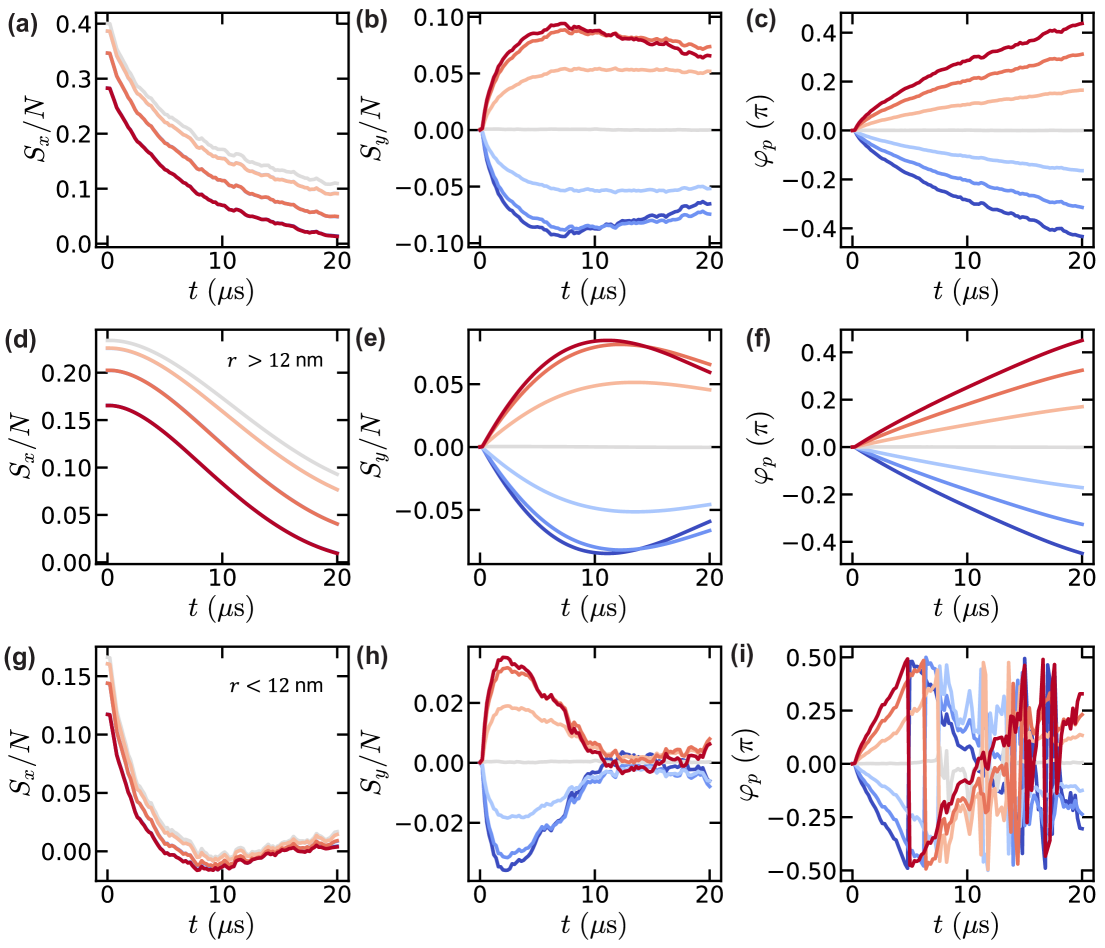
Figure 2: Numerical simulation of average twisting dynamics. We simulate the average twisting dynamics on a fully disordered system with $N=80$ spins by the cluster DTWA method. We plot the evolution of $S_{x}$, $S_{y}$ and $\varphi_{p}=\arctan(S_{y}/S_{x})$ for the full system (a-c), the subsystem consisting of the spins whose distance to the closest neighboring spin is larger than $12$ nm (d-f) and smaller than $12$ nm (g-i). The initial polarization is set as $80\%$. In all plots, different colors correspond to different initial rotation angles $\varphi_{o}$, ranging from $\varphi_{o}=-\pi/4$ (red) to $\varphi_{o}=\pi/4$ (blue).

IV.3 Dimer dynamics during quantum variance readout

Here, we analyze the effect of the dimers dynamics on the readout of the variance. Recall that the experiment protocol consists of two quenches: generation quench (with an evolution time $t_{\mathrm{g}}$) and readout quench (with an evolution time $t_{\mathrm{r}}$), with a $X_{\theta}$ rotation between the two quenches. Our discussion of one-axis twisting dynamics in the main text draws from the OAT picture, which maps well onto ordered spins in a lattice. In this picture, the twisting rate acts as a measurement of the variance of the spins.

Under the same pulse sequence, dimers behave distinctly but still contribute to the measured $\langle{S_{x}(t)}\rangle$ signal. The primary contribution of the dimers in our measurement is to alter the offset time $t_{\mathrm{o}}$ compared with the OAT case. As discussed in Sec. III, the decay of the spin length $\langle S_{x}(t_{\mathrm{r}})\rangle$ originates from the twisting of the spin projection noise around the Bloch sphere. Naively, when $\expectationvalue{S_{y}S_{z}}=0$, the spin length $S_{x}(t)$ reaches its maximum. While this is true for spins on a lattice, in the disordered system the time when $\expectationvalue{S_{y}S_{z}}=0$ does not coincide with the time at which $\expectationvalue{S_{x}(t)}$ is maximized, due to dimer dynamics.

The dimers always at least partially recover their polarization at $t_{\mathrm{r}}=t_{\mathrm{g}}$. Using Eq. (35), we can restrict the dynamics to the $\{\ket{++},\ket{--}\}$ subspace, such that $H_{\mathrm{XXZ}}=-J\quantity[\frac{1}{4}-\frac{\Sigma_{x}}{2}]$, where $\Sigma_{\mu}\ (\mu=x,y,z)$ is the Pauli operator in this subspace. For dimers initially prepared in $\ket{\psi(t_{\mathrm{g}}=0)}=\ket{++}$, the generation quench yields $\ket{\psi(t_{\mathrm{g}})}=\cos(Jt_{\mathrm{g}}/2)\ket{++}-i\sin(Jt_{\mathrm{g}}/2)\ket{--}$. After the rotation $X_{\theta}$, the state becomes $\ket{\psi(t_{\mathrm{g}},t_{\mathrm{r}}=0)}=\cos(Jt_{\mathrm{g}}/2)e^{i\theta}\ket{++}-i\sin(Jt_{\mathrm{g}}/2)e^{-i\theta}\ket{--}$. Finally, we evolve this quantum state under $H_{\mathrm{XXZ}}$ again for $t_{\mathrm{r}}$, i.e.,

$$\ket{\psi(t_{\mathrm{g}},t_{\mathrm{r}})} =\cos(\frac{t_{\mathrm{g}}}{2})e^{i\theta}\quantity[\cos(\frac{Jt_{\mathrm{r}}}{2})\ket{++}-i\sin(\frac{Jt_{\mathrm{r}}}{2})\ket{--}]$$ (39)

$$\ -i\sin(\frac{Jt_{\mathrm{g}}}{2})e^{-i\theta}\quantity[-i\sin(\frac{Jt_{\mathrm{r}}}{2})\ket{++}+\cos(\frac{Jt_{\mathrm{r}}}{2})\ket{--}]$$

$$=[\cos(\frac{Jt_{\mathrm{g}}}{2})\cos(\frac{Jt_{\mathrm{r}}}{2})e^{i\theta}-\sin(\frac{Jt_{\mathrm{g}}}{2})\sin(\frac{Jt_{\mathrm{r}}}{2})e^{-i\theta}]\ket{++}$$

$$\ +\quantity[-ie^{i\theta}\cos(\frac{Jt_{\mathrm{g}}}{2})\sin(\frac{Jt_{\mathrm{r}}}{2})-ie^{-i\theta}\sin(\frac{Jt_{\mathrm{g}}}{2})\cos(\frac{Jt_{\mathrm{r}}}{2})]\ket{--}.$$

As a result, the dimer contribution to the spin length is

$$\expectationvalue{S_{x}(t_{\mathrm{g}},t_{\mathrm{r}})} =\cos(Jt_{\mathrm{g}})\cos(Jt_{\mathrm{r}})-\sin(Jt_{\mathrm{g}})\sin(Jt_{\mathrm{r}})\cos(2\theta)$$ (40)

$$=\sin^{2}\theta\cos(J(t_{\mathrm{g}}-t_{\mathrm{r}}))+\cos^{2}\theta\cos(J(t_{\mathrm{g}}+t_{\mathrm{r}})).$$

In a system with positional disorder, dimers interact with different couplings $J=J_{0}/r_{12}^{3}$, where the inter-spin distance $r_{12}$ can be randomly sampled from Eq. (38). Most of the time ($t_{\mathrm{g}}\neq t_{\mathrm{r}}$), due to the random distribution of $J$, the dimers with different inter-spin distances oscillate between $\ket{++}$ and $\ket{--}$ with different frequencies, and $\expectationvalue{S_{x}(t_{\mathrm{g}},t_{\mathrm{r}})}$ averages to zero. However, when $t_{\mathrm{g}}=t_{\mathrm{r}}$, the first term in the equation above is no longer vanishing, i.e., $\expectationvalue{S_{x}(t_{\mathrm{g}},t_{\mathrm{g}})}=\sin^{2}\theta$ while the second term still averages to zero. Therefore, regardless of $\theta$, the dimers always partially recover their polarization at $t_{\mathrm{r}}=t_{\mathrm{g}}$. When $\theta=\pi/2$, we have $\expectationvalue{S_{x}(t_{\mathrm{g}},t_{\mathrm{g}})}=1$, indicating that the dimers fully recover their polarization. Indeed, we observe this feature in the experiment (see main text Fig. 2(e), inset). This feature fully originates from dimers, and is unrelated to spin projection noise of the collective spin wrapping around the Bloch sphere. While the offset time $t_{\mathrm{o}}$ is the time when the $\expectationvalue{S_{x}(t_{\mathrm{r}})}$ reaches its maximum for the OAT and lattice systems, we cannot use this as the procedure to identify $t_{\mathrm{o}}$ in the system with positional disorder. Instead, to determine $t_{\mathrm{o}}$, we use the condition that the state at $t_{\mathrm{r}}=t_{\mathrm{o}}$ should minimally wrap around the Bloch sphere, i.e., $\expectationvalue{S_{y}S_{z}}=0$.

References

- (1) Zu, C. et al. Emergent hydrodynamics in a strongly interacting dipolar spin ensemble. Nature 597, 45–50 (2021).
- (2) Liesen, J. & Strakos, Z. Krylov Subspace Methods: Principles and Analysis (Oxford University Press, 2012). URL https://doi.org/10.1093/acprof:oso/9780199655410.001.0001.
- (3) Kahanamoku-Meyer, G. D. & Wei, J. Gregdmeyer/dynamite: v0.4.0 (2024). URL https://doi.org/10.5281/zenodo.10906046.
- (4) Schachenmayer, J., Pikovski, A. & Rey, A. M. Many-Body Quantum Spin Dynamics with Monte Carlo Trajectories on a Discrete Phase Space. Physical Review X 5, 011022 (2015).
- (5) Block, M. et al. Scalable spin squeezing from finite-temperature easy-plane magnetism. Nature Physics 20, 1575–1581 (2024).
- (6) Alaoui, Y. A. et al. Measuring bipartite spin correlations of lattice-trapped dipolar atoms (2024). eprint 2404.10531.
- (7) Braemer, A., Vahedi, J. & Gärttner, M. Cluster truncated Wigner approximation for bond-disordered Heisenberg spin models. Physical Review B 110, 054204 (2024). eprint 2407.01682.
- (8) Nagao, K. & Yunoki, S. Two-dimensional correlation propagation dynamics with a cluster discrete phase-space method (2024). eprint 2404.18594.
- (9) Carleo, G. & Troyer, M. Solving the quantum many-body problem with artificial neural networks. Science 355, 602–606 (2017).
- (10) Haegeman, J. et al. Time-dependent variational principle for quantum lattices. Physical Review Letters 107, 070601 (2011).
- (11) Schmitt, M. & Heyl, M. Quantum many-body dynamics in two dimensions with artificial neural networks. Physical Review Letters 125, 100503 (2020).
- (12) Schmitt, M., Rams, M. M., Dziarmaga, J., Heyl, M. & Zurek, W. H. Quantum phase transition dynamics in the two-dimensional transverse-field ising model. Science Advances 8, eabl6850 (2022).
- (13) Sinibaldi, A., Giuliani, C., Carleo, G. & Vicentini, F. Unbiasing time-dependent variational monte carlo by projected quantum evolution. Quantum 7, 1131 (2023).
- (14) Vicentini, F. et al. Netket 3: Machine learning toolbox for many-body quantum systems. SciPost Physics Codebases 007 (2022).
- (15) Bradbury, J. et al. JAX: composable transformations of Python+NumPy programs (2018). URL http://github.com/google/jax.
- (16) Davis, E. J. et al. Probing many-body dynamics in a two-dimensional dipolar spin ensemble. Nature Physics 19, 836–844 (2023).