Robust Weight Imprinting: Insights from Neural Collapse and Proxy-Based Aggregation

Abstract

The capacity of a foundation model allows for adaptation to new downstream tasks. Weight imprinting is a universal and efficient method to fulfill this purpose. It has been reinvented several times, but it has not been systematically studied. In this paper, we propose a framework for imprinting, identifying three main components: generation, normalization, and aggregation. This allows us to conduct an in-depth analysis of imprinting and a comparison of the existing work. We reveal the benefits of representing novel data with multiple proxies in the generation step and show the importance of proper normalization. We determine those proxies through clustering and propose a novel variant of imprinting that outperforms previous work. We motivate this by the neural collapse phenomenon – an important connection that we can draw for the first time. Our results show an increase of up to 4% in challenging scenarios with complex data distributions for new classes.

1 Introduction

In machine learning applications, training models from scratch is often not viable due to limitations in data and compute. A popular solution is to apply transfer learning [1, 2] based on foundation models (FMs) [3] that are pre-trained on a large amount of data. A common approach in practice to adapt an FM to a novel task is to freeze its parameters and replace the output layer with a new head, e.g., for classification.

Imprinting.

Qi et al. [4] propose a simple solution for few-shot classification, called imprinting. Namely, the last-layer weight vector of a novel class is set to the normalized average of its scaled embedding vectors, i.e., its class mean. These class means are representatives of the classes, which we generally call proxies. This results in an efficient method without the need for gradient-based optimization. A plethora of studies have emerged surveying this technique by adding complexity and adaptability [5, 6, 7, 8, 9, 10, 11]. Despite many adaptations, imprinting lacks a systematic comparison that unifies them. Understanding its variations could unlock greater efficiency and performance across many fields, making the method even more versatile and impactful.

Framework.

We present a unifying framework that enables a systematic comparison of existing imprinting techniques. More precisely, we can generalize prior work by decomposing imprinting into three principal steps (see fig.˜1). During generation (GEN) of weights, the network selects representative data samples and generates one or more weight vectors per class (multiple proxies). Normalization (NORM) is crucial, as the network needs to balance its generated weight vectors. Aggregation (AGG) entails the computation of the final output, e.g., a class label.

The efficiency of imprinting enables us to perform a comprehensive analysis with a large number of experiments. We present a new, best-performing imprinting strategy using multi-modal weight imprinting in combination with the correct way of normalization.

Neural Collapse.

We investigate a recently discovered phenomenon called neural collapse [12], which provides a compelling explanation for why imprinting works. According to this phenomenon, when neural networks are trained to reach near-zero loss, their penultimate-layer embeddings collapse to the class means [12, 13]. Our investigation proves that a measurement of neural collapse provides insights about imprinting.

Contributions.

In summary, our main results and contributions are:

• We deconstruct weight imprinting into a framework composed of generation, normalization, and aggregation, and discuss variations for each of them, identifying prior work as special cases (section˜3). To the best of our knowledge, we are the first to conduct a comprehensive analysis of imprinting to this scale (section˜5).

• We present a new imprinting method utilizing $k$-means clustering for weight generation (section˜6.1) and show its benefits in certain few-shot scenarios (section˜6.2).

• To the best of our knowledge, we are the first to identify a connection between imprinting success and measures of neural collapse (section˜6.3).

We make the source code to reproduce our results publicly available.

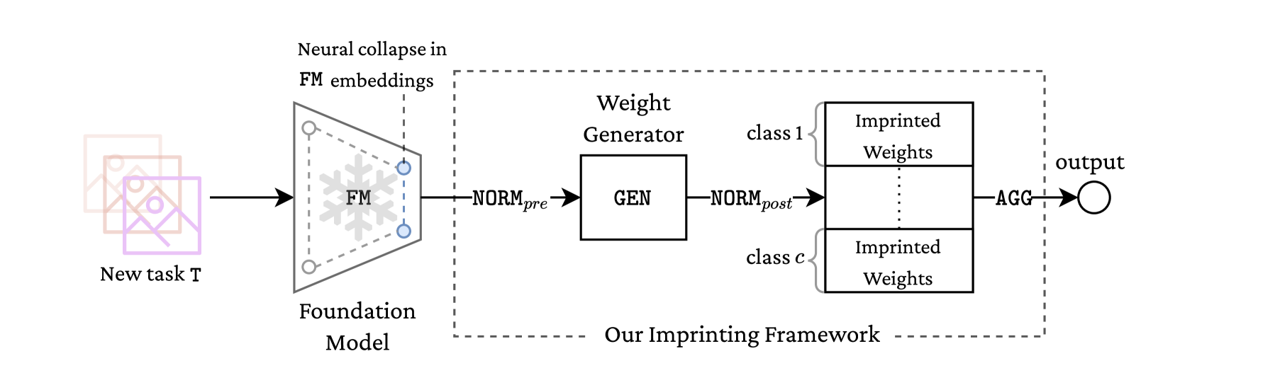
Figure 1: Overview of our imprinting framework. The foundation model FM is frozen and shows neural collapse. The weight generator (GEN) uses training data from a novel task T to generate one or more weight vectors (proxies) per class $1,\dotsc,c$. The final output of the test data in T is computed by an aggregation (AGG) mechanism. Embeddings and generated weights are normalized according to NORM_pre and NORM_post, respectively. During inference, embeddings are normalized according to NORM_inf (not shown here).

2 Related Work

Imprinting and Few-Shot Learning.

Weight imprinting was introduced in [4] for the few-shot learning scenario. It is implemented by setting the final layer weights for the novel classes to the scaled average of the embedding vectors of their training samples. Qi et al. [4] find that for up to $20$ samples, using a combination of imprinting and fine-tuning outperforms other state-of-the-art methods, including nearest neighbor algorithms. However, we are not limiting the number of samples and perform no fine-tuning on the imprinted weights to maintain efficiency. Imprinting has also been applied to object detection [5, 6], multi-label classification [8], semantic segmentation [10], and in combination with an attention mechanism to generate weights for the novel classes in a few-shot classification task [11].

Hosoda et al. [14] apply imprinting using quantile normalization to ensure statistical similarity between new and existing weights. We consider this as one normalization scheme in our framework. Zhang et al. [15] apply imprinting in chest radiography for detection of COVID-19 and find that it yields better results than joint gradient descent training of all classes when only few samples are available. They speculate whether normalization is a constraint in their imprinting model.

Before the era of deep learning, Mensink et al. [16] analyze the transferability of hand-crafted image features. They use a "nearest class multiple centroids" (NCMC) classifier with multiple proxies generated from a $k$-means clustering algorithm. In combination with metric learning, they compare favorably against the $m$-nearest neighbor algorithm. Our work, on the other hand, highlights efficient transfer learning provided by foundation models.

Transfer Learning.

Our work is related to the use of embedding vectors extracted with pre-trained models, which is one of the most straightforward transfer learning techniques, since the seminal works in computer vision [17] and natural language processing [18]. Kornblith et al. [19] showed that pre-training performance of a model is highly correlated with the performance of the resulting embedding vectors in downstream tasks. In addition, Huh et al. [20] provided insights into the required quality of pre-training data. Our work is orthogonal to these studies, since we focus on studying weight generation, normalization, and aggregation techniques applied later on for new task adaptation.

Continual Learning (CL).

Class means have also been used as proxies in CL. Although we investigate transfer learning scenarios, we review the imprinting applications and results from CL. Rebuffi et al. [21] dynamically select a subset of examples for each class and update internal representations via gradient descent. They use a nearest mean classifier (NMC) with respect to the saved examples. Janson et al. [22] use an NMC classifier as well and achieve good performance on CL benchmarks without any fine-tuning of the embeddings. However, they do not investigate the effect of normalization and using multiple proxies.

Findings of [23] show that a simple, approximate $m$-nearest neighbor classifier outperforms existing methods in an Online CL setting when all data can be stored. In our work, however, we compare imprinting all data to a limited number of more representative proxies striving for efficiency.

Neural Collapse (NC).

The phenomenon of NC was identified by [12] and refers to the convergence of the last-layer weight vectors to class means. It was shown that, regardless of the loss function, optimizer, batch-normalization, or regularization, NC will eventually occur (provided the training data has a balanced distribution) [13, 24, 25], but complete neural collapse is practically unrealistic [26]. In transfer learning, Galanti et al. [27] show that NC occurs on new samples and classes from the same distribution as the pre-training dataset, highlighting the usability of foundational models in such scenarios. In our work, we expand the survey on NC by experimenting with out-of-distribution classes belonging to different datasets and linking their degree of collapse to the success of certain imprinting strategies.

3 Imprinting Framework

In order to find out how to best set the classifier weights of a foundational model in downstream tasks T, we create a framework (see fig.˜1) that encompasses many different combinations, all of which work without gradient-based training. Thereby, we can unify all the existing imprinting strategies described in section˜2.

We analyze multi-class classification scenarios in that we do not separate into base and new classes, but focus on all classes in a novel T at the same time. To investigate the effect of the number of samples given, we look at n-shot ($n\in\mathbb{N}$) scenarios. For that, we randomly pre-sample the training data of T to $n$ samples per class – transitioning into the regime of few-shot learning.

Overview.

We analyze the effect of weight generation (GEN), normalizations ($\texttt{NORM}=\{\texttt{NORM}\textsubscript{{pre}},\texttt{NORM}\textsubscript{{post}},\texttt{NORM}\textsubscript{{inf}}\}$), and aggregation (AGG). The framework depicted in fig.˜1 consists of three main building blocks: a foundation model FM, a weight generator GEN, and extendable classifier weights that are imprinted. The FM remains frozen throughout the experiments. It receives data from T as inputs and produces embedding vectors. The training process generates weight vectors for each of the $c$ classes in T. Hereby, embeddings from the FM are normalized before the generation (GEN) step according to NORM_pre. The generated weight vectors per class are called proxies, prototypes, or representatives [28, 29, 30, 31]. These proxies are normalized according to NORM_post. As in [4], we do not use bias values. To classify the test data in T during inference, it is first embedded by the FM, normalized according to NORM_inf, and finally aggregated by AGG, resulting in a predicted class label.

Special Imprinting Cases.

Previously proposed imprinting methods can be defined as a special case of our framework. Figure˜4 in section˜6.1 provides an overview of existing imprinting strategies listed in literature for foundational models and benchmarks them with the new best-performing one we find through our framework. In total, we inspect all possible combinations (including variations in models, tasks, and seeds).

Weight Generation (GEN).

The purpose of GEN is to determine how the embeddings of the training data in T are used to form the new weights. In contrast to [4] which only incorporates one proxy per class (the mean), we add flexibility by allowing each class to have multiple proxies as in [16]. This enables non-linear classification. We denote the number of proxies as $k$, ranging between $1$ and the number of samples. We investigate the following operations conducted per class to generate its proxies:

• all: All embeddings (denoted as $k=\text{all}$).

• k-random: $k$ random embeddings.

• mean: The mean of all embeddings.

• k-means: $k$-means cluster centers. $k=1$ is the same as mean.

• k-medoids: $k$-medoids cluster centers.

• k-cov-max (covariance-maximization): Top $k$ embeddings by covariance.

• k-fps (farthest-point sampling): Iteratively selecting $k$ embeddings, such that it maximizes the distance from already selected ones (starting with random sample).

We choose this diverse list of methods to cover a wide range of approaches, ranging from heuristics (e.g., k-fps) to more complex algorithms (e.g., k-means). Note that only mean and k-means generate proxies that are not included in the given samples.

Normalization (NORM).

The main reason for applying normalization is to allow each embedding and weight vector to contribute equally on the same scale. The modes we allow are no normalization (none), $L^{2}$ normalization (L2), and quantile normalization (quantile).

L2 normalization can be applied to embeddings before GEN via NORM_pre, to the generated weights via NORM_post, and to embeddings in inference via NORM_inf. In any case, the vector is $L^{2}$-normalized by dividing it by its Euclidean $\|\cdot\|_{2}$ length.

quantile normalization [32, 33] can only be applied to generated weights. This non-linear operation distributes weights equally. Recall that if more than one class is contained in T ($c>1$), GEN is performed for each class, and the reference distribution changes accordingly. In particular, for the first class there is no reference distribution to map to. This is different from [14], where new weights are matched to the distribution of the original classifier weights of the FM. Since we do not consider the classes used for pre-training the FM and especially do not assume access to their last-layer weights, this is not possible in our scenario.

Aggregation (AGG).

There are various ways to use the generated weights per class during inference, especially when $k>1$. We focus on two different modes, max and m-nn. The former, max, computes the inner product of the input embedding and the imprinted weights and outputs the class label with the maximum activation. The latter, m-nn, uses the class weights as keys and the embeddings as values, and chooses the final winning output class via the $m$-nearest neighbor algorithm. The m-nn voting is weighted by the inverse of the distances to their nearest neighbor, turning it into weighted majority voting.

Note that max is the same as 1-nn in the case of L2 for NORM_post, since for any fixed embedding vector $v$ and variable proxy $w$, the argmin of $\|v-w\|^{2}=\|v\|^{2}-2\langle v,w\rangle+\|w\|^{2}$, calculated by 1-nn, is the same as the argmax of the inner product $\langle v,w\rangle$ calculated in max.

4 Measurement of Neural Collapse

Neural collapse (NC) [12] refers to the phenomenon that occurs on the last-layer classifier weights of neural networks in the terminal phase of training (TPT). When the network is trained well beyond zero training error, the learned embeddings of each class, assuming balanced classes, collapse to their class means. These globally centered class means and classifier weights form a simplex equiangular tight frame (ETF) – a collection of equal length and maximally equiangular vectors, that maximize the between-class variability. This results in an optimal linearly separable state for classification. In fig.˜2 (left), we illustrate the collapse of a FM on its pre-training data. The newly arrived data T from a different dataset is distributed more unevenly across the embedding space (right).

Two important characteristics of NC are variability collapse, i.e., the within-class variability of the penultimate-layer embeddings collapses to zero, and convergence to nearest-mean-classification. We focus on variability collapse ($\mathcal{NC}_{1}$), using the equation 1 from [13]:

$$\mathcal{NC}_{1}=\tfrac{1}{c}\mathrm{trace}(\Sigma_{W}{\Sigma^{+}_{B}}),$$ (1)

where $\Sigma_{W},\Sigma_{B}\in\mathbb{R}^{l\times l}$ are within- and between-class covariance matrices, respectively, $l$ is the dimension of the embedding vector, $c$ is the number of classes, and ⁺ symbolizes the pseudo-inverse. Based on the equation, an $\mathcal{NC}_{1}$ score closer to zero signifies a higher collapse. In contrast, an increase in multi-modality of data leads to a higher $\mathcal{NC}_{1}$ score (as analyzed in fig.˜11). Note that this measurement is not independent of the embedding dimension $l$ and the number of classes $c$. According to NC, imprinting the mean, as originally done in [4], is best when $\mathcal{NC}_{1}$ is small. We claim that when the data is not fully collapsed (as is often the case in practice), the scale of $\mathcal{NC}_{1}$ could guide the proxy generation method, e.g., having multiple proxies $k>1$ per class. We investigate this in section˜6.3.

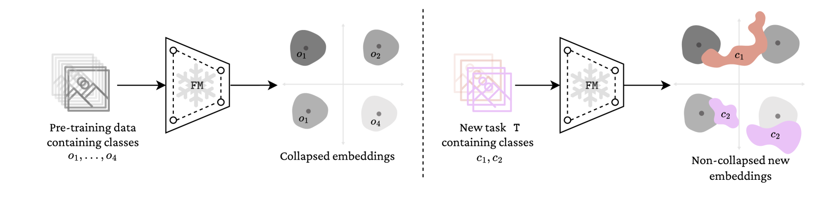
Figure 2: Left: The embeddings of the pre-training data, after being used to train the foundation model FM, show neural collapse, as each class ($o_{1},\dotsc,o_{4}$) is evenly separated in space and accumulates around their respective class means. Right: For a novel task with classes $c_{1},c_{2}$ (pink and brown) scatter around the collapsed pre-trained classes (gray).

5 Experimental Setup

Models.

We use resnet18 [34] and vit_b_16 [35] as FMs, one CNN-based and one Transformer-based architecture. In neural collapse investigations (section˜6.3), we also use resnet50 [34] and swin_b [36]. All of them are pre-trained on ImageNet-1K (ILSVRC 2012) [37]. To generate the embeddings, we use PyTorch’s torchvision models.

Tasks.

To find out the best imprinting strategy within our framework, we focus on tasks T created from the datasets MNIST [38], FashionMNIST [39], and CIFAR-10 , each containing 10 classes. We mainly focus on the three T containing all ten classes. Furthermore, we look at smaller tasks only containing classes $\{0,1,2\}$, and the two tasks containing classes $\{1,3,5,7,9\}$ resp. $\{0,2,4,6,8\}$. This random selection of $3\cdot 4=12$ tasks adds variation to our evaluation.

In the investigations of neural collapse (NC), we also look at the FMs’ pre-training data (ImageNet). As its test set is not available, we use its validation set in $\mathcal{NC}_{1}$ computations. For ImageNet, we relabel data by combining multiple classes into one label to simulate multi-modal class distributions for an in-depth NC analysis. These tasks are called "$d$ in $1$", $d=1,\dotsc,10$, each containing $10$ different labels. More precisely, we take 100 random classes from ImageNet and sequentially map the first $d$ to label $1$, the second $d$ to label $2$, etc., until we reach 10 distinct labels. See fig.˜3 for a simplified example. We do this random sampling 10 times which results in $10\cdot 10=100$ tasks.

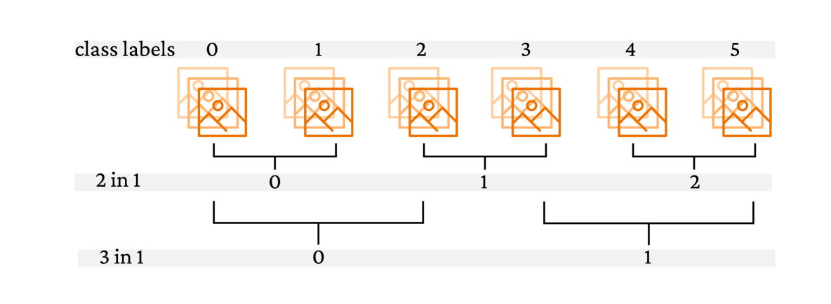
Figure 3: Combining multiple classes into one to create tasks with multi-modal class distributions. Example: "$d$ in 1", $d=2,3$.

Scale.

In total, we run approximately 350 000 experiments, varying across the imprinting components, foundation models, tasks, and seeds. This is feasible with minimal effort as imprinting is a highly efficient method that operates without relying on gradient descent or other non-linear optimization techniques.

Evaluation.

Throughout our experiments, the median accuracy on the test set for three different seeds is reported, if not otherwise specified. In sections˜6.1 and 6.2, we investigate the imprinting performance by varying the FM (2) and T (12). We then sort the combinations by their final accuracy. There are $2\cdot 12=24$ potentially different ranks for each of the combinations. We show the average rank, average accuracy, and statistical significance in ranking (dis-)agreements through critical difference (CD) diagrams as presented in [40]. In the CD diagrams, a thick horizontal line indicates a group of combinations that are not significantly different from each other in terms of accuracy. We consider differences significant if $p<0.05$.

In experiments with neural collapse (section˜6.3), we investigate four FMs on 100 ImageNet tasks and the three tasks containing all of MNIST, FashionMNIST, and CIFAR-10, respectively.

6 Results

Our main experimental insights are:

1. Our imprinting framework generalizes previous methods, and we find a new superior imprinting strategy (section˜6.1).

2. We show that our strategy is beneficial in few-shot scenarios with as little as 50 samples per class (section˜6.2).

3. We identify a correlation between imprinting success utilizing multiple proxies and measures of neural collapse (section˜6.3).

6.1 Best Imprinting Strategy

Paper	NORMpre	GEN	NORMpost	NORMinf	AGG	Avg. acc. %
Qi et al. [4]	L2	mean	L2	L2	max	87.72
Hosoda et al. [14]	none	mean	quantile	none	max	82.15
Janson et al. [22]	none	mean	none	none	1-nn	87.65
Ours	L2	k-means	L2	L2	max	91.47

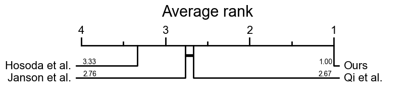
[table]A table beside a figure

Figure 4: Previously studied imprinting strategies are special cases within our framework. The framework enables the creation of a novel configuration ("Ours") that outperforms previous work across FMs and Ts by a large margin with statistical significance. Here, $k=20$ is chosen.

We provide a comparison between memory-constrained methods used for imprinting on foundation models in fig.˜4, namely, [4, 14, 22], as well as a novel configuration that results from our framework which we call “Ours”. We investigate the impact of using m-nn aggregation on all data afterward. We focus on $k=20$ and find that our method, consisting of k-means weight generation, L2 normalizations, and max aggregation, outperforms all other approaches by a margin of $4\%$ with statistical significance, as can be seen in the CD diagram. Below, we analyze each of the components of the framework separately.

Weight Generation (GEN).

To analyze the impact of GEN, we first focus on the max aggregation. For the weight generation analysis, we do not fix NORM, but simply show the run with the best NORM combination, if not otherwise specified. The m-nn aggregation and different values for NORM are analyzed later in this section.

GEN	$k$	Avg. acc. %
k-means	20	91.95
k-medoids	20	87.31
mean	1	87.76
k-cov-max	20	84.74
k-random	20	82.79
k-fps	2	63.90

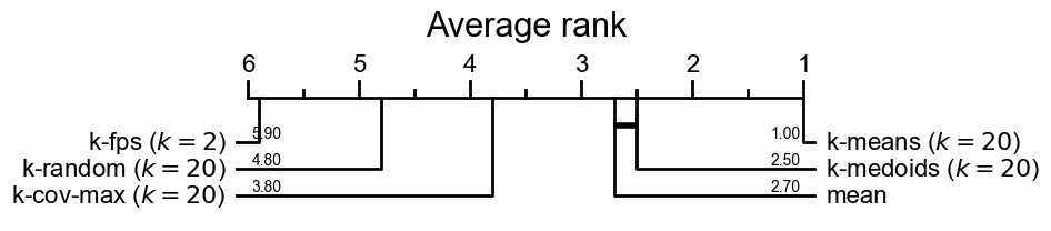
[table]A table beside a figure

Figure 5: Benchmarking GEN mechanism for $k\leq 20$ across FMs and Ts. Best NORM combination for each row used implicitly. AGG is fixed to max. CD diagram proves that k-means weight generation is significantly better than all other methods.

Initially, we limit the number of generated proxies ($k\leq 20$). Results in fig.˜5 show how k-means, using as many proxies as possible (in this case, $20$) outperforms by $4\%$ on average accuracy compared to all the other GEN methods. The CD diagram illustrates its statistical significance in ranking. Furthermore, while k-medoids with $20$ proxies is computationally expensive, it is statistically on par with mean, and covariance maximization, furthest-point sampling and random selection show even weaker performances. We find similar results for $k\leq 5$, where k-means outperforms the other methods as well (see fig.˜13).

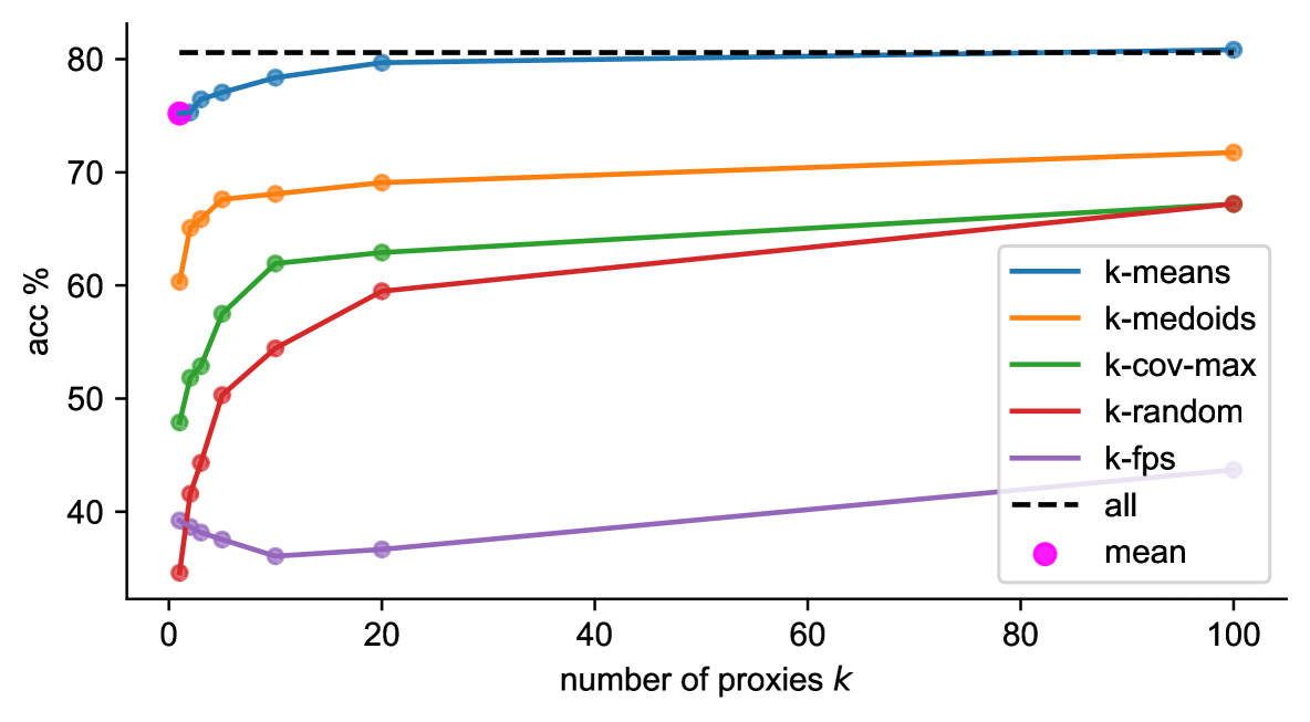
Figure 6: Benchmarking different GEN methods with resnet18 on CIFAR-10. All combinations employ L2 for all NORM.

As the number of proxies ($k$) increases, k-means continues to be the best GEN method. An example for resnet18 and CIFAR-10 can be found in fig.˜6. All methods converge towards the point of imprinting (saving) all data ($k=\text{all}$), even surpassing it in the case of k-means. Due to its superior performance, we mainly focus on k-means in the remainder of the analysis.

Normalization (NORM).

To investigate the role of normalization, we compare all the different NORM methods, focusing on k-means as GEN with $k=1,5,20$. For $k=1$ and varying NORM_post (while taking best values for NORM_pre and NORM_inf implicitly), fig.˜7 shows that for weight normalization, L2 is by far the best choice. quantile and none normalization perform significantly worse.

NORMpost	Avg. acc. %
L2	87.76
quantile	80.71
none	84.03

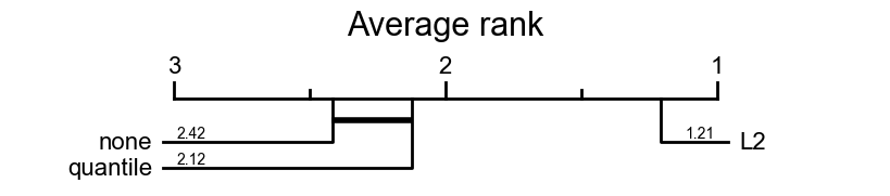
[table]A table beside a figure

Figure 7: Benchmarking NORM_post mechanism across FMs and Ts. The best NORM_pre and NORM_inf combinations for each row are used implicitly. GEN is fixed to mean (that is, $k=1$) and AGG is fixed to max. The CD diagram shows the statistical significance of L2 as weight normalization NORM_post.

NORMpre	NORMinf	Avg. acc.
none	L2	87.76
none	none	88.36
L2	L2	87.72

Table 1: Benchmarking NORM_pre and NORM_inf mechanisms across FMs and Ts. NORM_post is fixed to L2, GEN to mean, and AGG to max. No statistically significant differences were found.

Keeping L2 for NORM_post fixed, we find no statistical differences between the different combinations of NORM_pre and NORM_inf. Its performances can be found in table˜1. For larger values of $k$, the differences among NORM_post become even more pronounced, but for NORM_pre and NORM_inf, it stays statistically indifferent for L2 weight normalization (see tables˜2 and 14 for all combinations at once with $k=1$, and tables˜3 and 15 for $k=20$).

Henceforth, we limit all the succeeding experiments to Qi’s [4] normalization, that is, using L2 for all NORM. We choose this combination of normalizations to specifically capture cosine similarity in max aggregation.

Aggregation (AGG).

In addition to max, we study the effect of m-nn as an aggregation method. Recall that max is a special case of m-nn when $m=1$ (as NORM_post is set to L2). We investigate different values for $m\in\{1,3,5,20,50\}$.

AGG	Avg. acc. %
5-nn	93.86
3-nn	93.67
20-nn	93.73
1-nn	92.97
max	92.97
50-nn	93.15

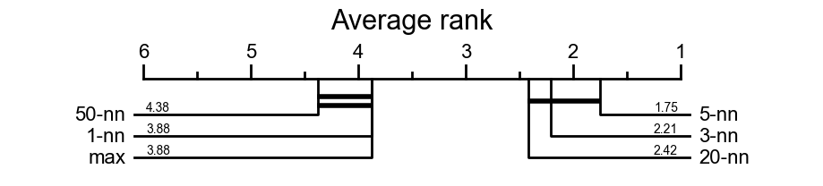
[table]A table beside a figure

Figure 8: Benchmarking AGG mechanism across FMs and Ts. GEN is fixed to all ($k=\text{all}$), that is, imprinting (saving) all data to weights. L2 normalization is used for all NORM. The CD diagram shows statistical significance of 3-nn, 5-nn, and 20-nn over max aggregation.

When all data is imprinted, fig.˜8 shows that using m-nn aggregation for $m\in\{3,5,20\}$ is slightly better than max.

AGG	Avg. acc. %
1-nn	91.47
max	91.47
3-nn	90.97
5-nn	90.54
20-nn	87.57

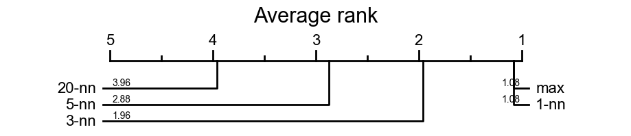
[table]A table beside a figure

Figure 9: Benchmarking AGG mechanism across FMs and Ts. GEN is fixed to k-means with $k=20$. L2 normalization is used for all NORM. The CD diagram shows that max is the best-performing aggregation method.

With $k=20$ and k-means as GEN, max ($=$1-nn) aggregation becomes the top performing combination (see fig.˜9). Furthermore, the reduction of proxies (from all $\approx 6000$ per class to $k=20$) leads to a minor decrease in accuracy of around $2\%$.

6.2 Few-Shot Scenario

We analyze the n-shot scenario with our method, that is, k-means as GEN, L2 normalizations, and max as AGG. Furthermore, we focus on the large tasks T, that contain ten classes at once. In this scenario, due to sampling only a few examples ($n$), we average over five different seeds.

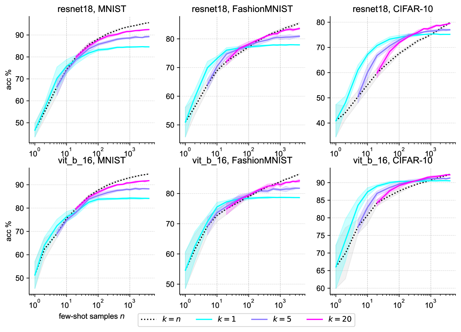
Figure 10: k-means with different values for $k$ in n-shot scenarios. $95\%$ confidence intervals are shown in shaded colors. Other variables are fixed to our previously described best method of using L2 normalizations and max as AGG. Note that only data for the meaningful case of $k\leq n$ is shown. It can be inferred that for MNIST and FashionMNIST, mean is not the best strategy anymore starting at roughly 50 samples.

From the results shown in fig.˜10, we find that as the number of samples $n$ increases, k-means starts outperforming mean imprinting. The usage of a higher number of proxies $k$ results in even greater performance. This shift occurs at roughly 50 samples per class for MNIST and FashionMNIST, while for CIFAR-10, $k>1$ becomes prominently better at around 200 samples per class (see fig.˜16 for a focus on $10\leq n\leq 200$).

6.3 Neural Collapse and Number of Proxies

Figure˜11 depicts the neural collapse measurement $\mathcal{NC}_{1}$ (see eq.˜1) for the three tasks containing all of MNIST, FashionMNIST, CIFAR-10, as well as the 100 ImageNet tasks with remapped labels as explained in section˜5. We can see that ImageNet has a close-to-zero $\mathcal{NC}_{1}$ score, which increases linearly when adding more classes to each label (i.e., increasing multi-modality). As for other datasets, CIFAR-10 is generally more collapsed according to its low value of $\mathcal{NC}_{1}$. We hypothesize that this is due to the similarity of its categories to those appearing in ImageNet. Apart from that, the $\mathcal{NC}_{1}$ for Transformer-based architectures is much lower and therefore they are more collapsed compared to the CNN-inspired FMs. Architectural differences are further explained in section˜A.2.

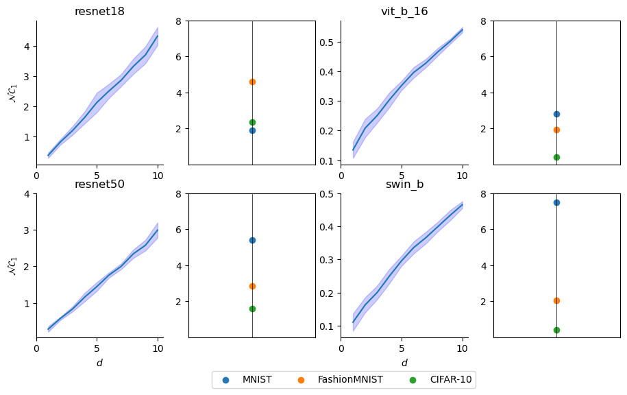
Figure 11: Average $\mathcal{NC}_{1}$ and $95\%$ confidence intervals of ten random ImageNet label remappings ("$d$ in $1$") for every $d=1,\dotsc,10$. The $\mathcal{NC}_{1}$ for the tasks containing all of MNIST, FashionMNIST, and CIFAR-10 at once are depicted in dots. When compared to the $\mathcal{NC}_{1}$ on the pre-training set (ImageNet), these sets are less collapsed on the Transformer-based architectures. A clear linear relationship across $d$ can be inferred for all FMs, i.e., increased multi-modality implies less collapse.

For the same data, fig.˜12 depicts accuracy over a varying number of proxies $k$ inferred from k-means. A prominent peak at $k=d$ can be inferred for every FM, and reflects that $d$ class proxies lead to the best result for $d$-modal class distributions. The fact that CIFAR-10 has the lowest $\mathcal{NC}_{1}$ (see fig.˜11) is reflected by flat curves over $k$. This confirms that the $\mathcal{NC}_{1}$ score is a significant indicator of multi-modality. Namely, a higher $\mathcal{NC}_{1}$ score indicates the benefits of using a higher number of proxies.

Furthermore, increasing $k$ for the ImageNet sets has a much larger effect on the CNN-based models. We argue that this is because of their higher values of $\mathcal{NC}_{1}$ and investigate this more deeply in section˜A.2.

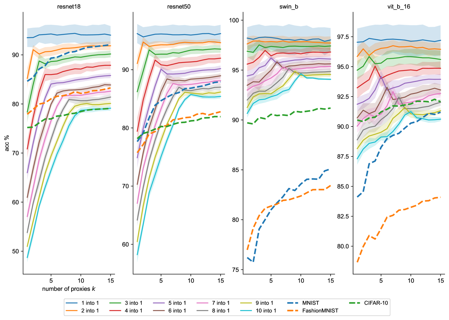
Figure 12: Averaged accuracy of ten random ImageNet label remappings ("$d$ in $1$") for every $d=1,\dotsc,10$ over number of proxies $k$ used for k-means in GEN. $95\%$ confidence intervals are shown in shaded colors. L2 for all NORM and max as aggregation are used. Accuracies of the tasks containing all of MNIST, FashionMNIST, and CIFAR-10 at once are shown in dotted lines. In all four plots, peaks in accuracy at $k=d$ can be inferred. This confirms the connection between the effect of using multiple proxies and the collapse of the data.

7 Discussion

We present a new framework to analyze the three main components relevant to weight imprinting, namely, weight generation, normalization, and aggregation. Within this framework, state-of-the-art imprinting strategies become special cases. This allows for a comprehensive analysis of different approaches through systematic experiments and leads us to generalize to a new, best-performing imprinting strategy. That is, using k-means weight generation with L2 normalizations and max aggregation outperforms all previously studied methods (see fig.˜4).

k-means generates better weights than mean.

In particular, we find that the mean weight generation (GEN) method, despite its prominence in previous work, falls short compared to k-means – even when the number of proxies $k$ is very small. Remarkably, with as little as 50 samples per class, k-means can already outperform the original imprinting method proposed in [4], highlighting its advantage in few-shot scenarios.

L2 weight normalization is essential for strong performance.

The max aggregation directly scales with the magnitude of the weights. Normalization (NORM_post) ensures that all class weights contribute equally to the output. Nearest neighbor (l-nn) aggregation is not as affected by the lack of normalization, since it uses Euclidean distance. Although still part of common procedure, normalizations for embeddings (NORM_pre and NORM_inf) appear to have minimal impact on performance.

With max aggregation, there is no need to store all data.

While nearest neighbor (m-nn) aggregation (AGG) performs well when all data is saved (e.g., when there are no storage constraints), max aggregation with limited number of representative proxies (e.g., $k$-means) is an efficient alternative without a substantial loss in performance.

Neural collapse proves the efficacy of imprinting.

During training, the last-layer weights of a FM collapse to their respective class means. This proves the success of mean imprinting on known classes. New, out-of-distribution data, however, often shows less collapse, making it beneficial to imprint more than one proxy.

Limitations.

Since our experiments are limited to a small selection of foundation models and tasks, running additional experiments could strengthen the statistical significance. While imprinting alone provides an efficient solution to transfer learning, we do not investigate the benefit of combining it with optimization methods like gradient-based learning when more samples become available. This combination could use imprinting as initialization or apply metric learning to improve imprinting capabilities.

Future Work.

The usage of both weight and activation sparsity as in [42] could change the within- and between-class variability in favor of using a higher number of proxies. Synaptic intelligence approaches like the weight saturation presented in this work are paths of further study. We use the penultimate layer embeddings for generating the classifier weights. An interesting area of study could be extracting embeddings from previous layers of the FM for this purpose. Lately, the study in [43] showed that adding a multi-layer perceptron projector between the penultimate and classification layers results in representations that are more transferable. Apart from that, it would be interesting to imprint the weights of other layers as well (see, for example, [10]).

8 Conclusion

We investigated imprinting as an efficient method for transfer learning based on foundation models. Within our new framework, we found a new imprinting strategy that outperforms all previously studied ones. The phenomenon of neural collapse provides theoretical proof for its success.

Author Contributions

JW contributed to the development of the framework, conducting experiments and evaluated the findings. GA was responsible for investigating NC measures and overall contribution to the project. MK contributed to extending the framework and handling data preparation. AF provided critical feedback on the presentation of the results and contributed to refining the manuscript. AL, ER, and FG provided supervision, contributed to the overall concepts presented, and to refining the manuscript.

Appendix A Appendix

A.1 Additional Tables and Critical Difference Diagrams

We provide additional tables and critical difference (CD) diagrams that are referenced and put into context in the main paper.

GEN	$k$	Avg. acc. %
k-means	5	89.57
mean	1	87.76
k-medoids	5	85.59
k-cov-max	5	82.83
k-random	5	76.41
k-fps	2	63.90

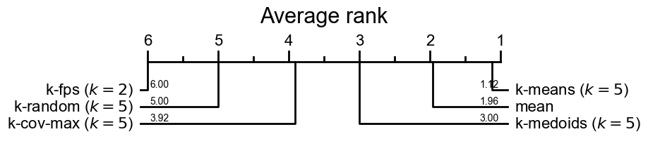
[table]A table beside a figure

Figure 13: Benchmarking GEN mechanism for $k\leq 5$ across FMs and Ts. Best NORM combination for each row is used implicitly. AGG is fixed to max. CD diagram depicts statistical significance of k-means as GEN. See fig.˜5 for $k\leq 20$.

NORMinf	NORMpre	NORMpost	Avg. acc. %
L2	none	L2	87.76
none	none	L2	87.76
L2	L2	L2	87.72
L2	L2	quantile	80.71
none	none	quantile	80.72
L2	none	quantile	80.72
L2	L2	none	84.03
L2	none	none	73.75
none	none	none	73.75

Table 2: Benchmarking NORM across FMs and Ts shows crucial effect of L2 normalization. GEN is fixed to mean and AGG to max. See fig.˜14 for average ranks.

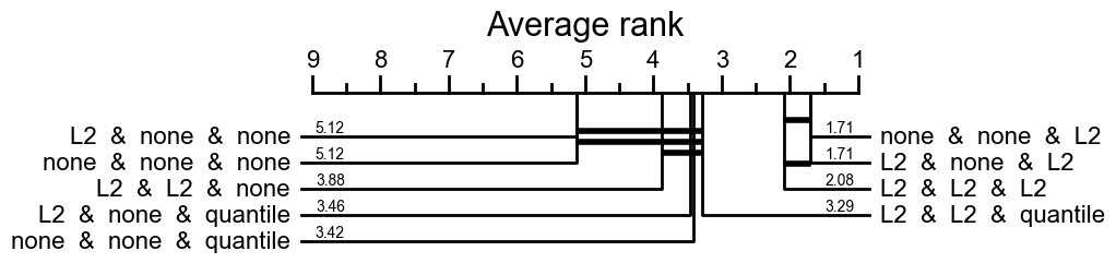
Figure 14: CD diagram depicting statistical significance of L2 for NORM_post. Combinations are listed as "NORM_inf & NORM_pre & NORM_post". See table˜2 for further details and average accuracies.

NORMinf	NORMpre	NORMpost	Avg. acc. %
L2	L2	L2	91.47
L2	none	L2	91.45
none	none	L2	91.45
L2	L2	quantile	90.91
L2	L2	none	89.97
L2	none	quantile	79.84
none	none	quantile	79.84
L2	none	none	79.24
none	none	none	79.24

Table 3: Benchmarking NORM across FMs and Ts. GEN is fixed to k-means with $k=20$ and AGG to max. See fig.˜15 for average ranks.

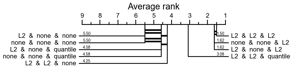
Figure 15: CD diagram depicting statistical significance of L2 for NORM_post. Combinations are listed as "NORM_inf & NORM_pre & NORM_post". See table˜3 for further details and average accuracies.

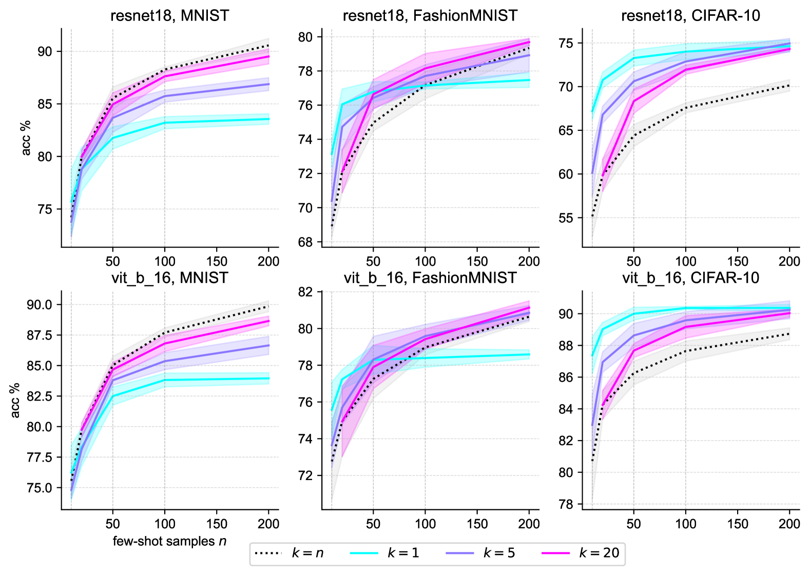
Figure 16: k-means with different values for $k$ in n-shot scenarios with focus on $10\leq n\leq 200$. $95\%$ confidence intervals shown in shaded colors. Other variables are fixed to our previously described best method of using L2 for NORM and max as AGG. Note that only data for the meaningful case of $k\leq n$ is shown. It can be inferred that for MNIST and FashionMNIST, mean is not the best strategy anymore starting at roughly 50 samples. See fig.˜10 for more values of $n$.

A.2 Differences between Foundation Models

While an in-depth comparison of foundation models is beyond the scope of this paper, we believe it is important to highlight key observations. In particular, fig.˜11 shows significantly lower $\mathcal{NC}_{1}$ scores for vit_b_16 and swin_b on their pre-training ImageNet data compared to the resnet models. We hypothesize that this difference is primarily due to model size and training regimes. The Transformer-based architectures (vit_b_16 and swin_b) have a considerably higher parameter count ($\approx 87$M) than the resnet models (11.7M and 25.6M, respectively). Additionally, vit_b_16 and swin_b were trained for three times as many epochs (300 vs. 90) while using a substantially lower learning rate (0.003 and 0.01 vs. 0.1). Notably, the embedding dimensions of these models are comparable, meaning that the observed differences in $\mathcal{NC}_{1}$ scores cannot be attributed to differences in representation dimensionality. Instead, we argue that the combination of larger model size, extended training duration, and lower learning rates likely contributes to greater overfitting, leading to more pronounced collapse.

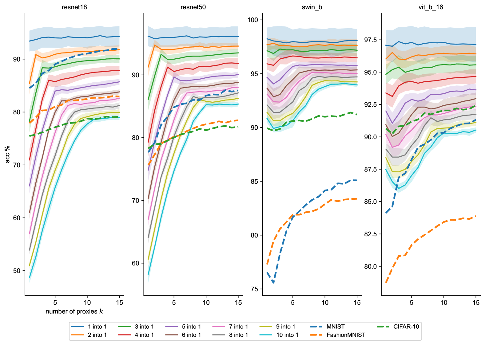
Figure 17: Averaged accuracy of ten random ImageNet label remappings ("$d$ in $1$") for every $d=1,\dotsc,10$ over number of proxies $k$ used for k-means in GEN. $95\%$ confidence intervals are shown in shaded colors. We set NORM_post and NORM_inf to L2, and NORM_pre to none. Accuracies of the tasks containing all of MNIST, FashionMNIST, and CIFAR-10 at once are shown in dotted lines. Besides the prominent peaks in accuracy at $k=d$ (as already observed in fig.˜12), a consistent dip between $k=1$ and $k=d$ appears in Transformer-based models.

Figure˜17, similar to fig.˜12, illustrates the impact of varying the number of proxies on imprinting accuracy across different foundation models (FMs). The key difference in this figure is the use of none for NORM_pre instead of L2. This seemingly minor change reveals a striking contrast between CNN- and Transformer-based architectures: a distinct and consistent dip between $k=1$ and $k=d$ appears in Transformer-based models, whereas this dip is absent in fig.˜12, where L2 is used as NORM_pre, and does not occur at all in the resnet models. We hypothesize that this difference arises from the distinct embedding distributions of CNN and Transformer architectures (see, e.g., [14, Figure S2]).

References

- Bengio [2012] Yoshua Bengio. Deep learning of representations for unsupervised and transfer learning. In Proceedings of ICML workshop on unsupervised and transfer learning, pages 17–36. JMLR Workshop and Conference Proceedings, 2012.
- Yosinski et al. [2014] Jason Yosinski, Jeff Clune, Yoshua Bengio, and Hod Lipson. How transferable are features in deep neural networks? Advances in neural information processing systems, 27, 2014.
- Bommasani et al. [2021] Rishi Bommasani, Drew A Hudson, Ehsan Adeli, Russ Altman, Simran Arora, Sydney von Arx, Michael S Bernstein, Jeannette Bohg, Antoine Bosselut, Emma Brunskill, et al. On the opportunities and risks of foundation models. arXiv preprint arXiv:2108.07258, 2021.
- Qi et al. [2018] Hang Qi, Matthew Brown, and David G Lowe. Low-shot learning with imprinted weights. In Proceedings of the IEEE conference on computer vision and pattern recognition, pages 5822–5830, 2018.
- Li et al. [2021] Yiting Li, Haiyue Zhu, Jun Ma, Sichao Tian, Chek Sing Teo, Cheng Xiang, Prahlad Vadakkepa, and Tong Heng Lee. Classification weight imprinting for data efficient object detection. In 2021 IEEE 30th International Symposium on Industrial Electronics (ISIE), pages 1–5. IEEE, 2021.
- Yan et al. [2023] Dingtian Yan, Jitao Huang, Hai Sun, and Fuqiang Ding. Few-shot object detection with weight imprinting. Cognitive Computation, 15(5):1725–1735, 2023.
- Passalis et al. [2020] Nikolaos Passalis, Alexandros Iosifidis, Moncef Gabbouj, and Anastasios Tefas. Hypersphere-based weight imprinting for few-shot learning on embedded devices. IEEE Transactions on Neural Networks and Learning Systems, 32(2):925–930, 2020.
- Khan et al. [2021] Mina Khan, P Srivatsa, Advait Rane, Shriram Chenniappa, Asadali Hazariwala, and Pattie Maes. Personalizing pre-trained models. arXiv preprint arXiv:2106.01499, 2021.
- Cristovao et al. [2022] Paulino Cristovao, Hidemoto Nakada, Yusuke Tanimura, and Hideki Asoh. Few shot model based on weight imprinting with multiple projection head. In 2022 16th International Conference on Ubiquitous Information Management and Communication (IMCOM), pages 1–7. IEEE, 2022.
- Siam et al. [2019] Mennatullah Siam, Boris N Oreshkin, and Martin Jagersand. Amp: Adaptive masked proxies for few-shot segmentation. In Proceedings of the IEEE/CVF International Conference on Computer Vision, pages 5249–5258, 2019.
- Gidaris and Komodakis [2018] Spyros Gidaris and Nikos Komodakis. Dynamic few-shot visual learning without forgetting. In Proceedings of the IEEE conference on computer vision and pattern recognition, pages 4367–4375, 2018.
- Papyan et al. [2020] Vardan Papyan, XY Han, and David L Donoho. Prevalence of neural collapse during the terminal phase of deep learning training. Proceedings of the National Academy of Sciences, 117(40):24652–24663, 2020.
- Zhu et al. [2021] Zhihui Zhu, Tianyu Ding, Jinxin Zhou, Xiao Li, Chong You, Jeremias Sulam, and Qing Qu. A geometric analysis of neural collapse with unconstrained features. Advances in Neural Information Processing Systems, 34:29820–29834, 2021.
- Hosoda et al. [2024] Kazufumi Hosoda, Keigo Nishida, Shigeto Seno, Tomohiro Mashita, Hideki Kashioka, and Izumi Ohzawa. A single fast hebbian-like process enabling one-shot class addition in deep neural networks without backbone modification. Frontiers in Neuroscience, 18:1344114, 2024.
- Zhang et al. [2021] Jianxing Zhang, Pengcheng Xi, Ashkan Ebadi, Hilda Azimi, Stéphane Tremblay, and Alexander Wong. Covid-19 detection from chest x-ray images using imprinted weights approach. arXiv preprint arXiv:2105.01710, 2021.
- Mensink et al. [2013] Thomas Mensink, Jakob Verbeek, Florent Perronnin, and Gabriela Csurka. Distance-based image classification: Generalizing to new classes at near-zero cost. IEEE transactions on pattern analysis and machine intelligence, 35(11):2624–2637, 2013.
- Donahue et al. [2014] Jeff Donahue, Yangqing Jia, Oriol Vinyals, Judy Hoffman, Ning Zhang, Eric Tzeng, and Trevor Darrell. DeCAF: A Deep Convolutional Activation Feature for Generic Visual Recognition. In ICML, pages 647–655, 2014.
- Devlin et al. [2019] Jacob Devlin, Ming-Wei Chang, Kenton Lee, and Kristina Toutanova. BERT: Pre-training of Deep Bidirectional Transformers for Language Understanding. In NAACL-HLT, pages 4171–4186, 2019.
- Kornblith et al. [2019] Simon Kornblith, Jonathon Shlens, and Quoc V. Le. Do Better ImageNet Models Transfer Better? In CVPR, pages 2656–2666, Long Beach, CA, USA, 2019. IEEE.
- Huh et al. [2016] Minyoung Huh, Pulkit Agrawal, and Alexei A. Efros. What makes ImageNet good for transfer learning?, 2016. arXiv:1608.08614.
- Rebuffi et al. [2017] Sylvestre-Alvise Rebuffi, Alexander Kolesnikov, Georg Sperl, and Christoph H Lampert. icarl: Incremental classifier and representation learning. In Proceedings of the IEEE conference on Computer Vision and Pattern Recognition, pages 2001–2010, 2017.
- Janson et al. [2022] Paul Janson, Wenxuan Zhang, Rahaf Aljundi, and Mohamed Elhoseiny. A simple baseline that questions the use of pretrained-models in continual learning. In NeurIPS 2022 Workshop on Distribution Shifts: Connecting Methods and Applications, 2022.
- Prabhu et al. [2023] Ameya Prabhu, Zhipeng Cai, Puneet Dokania, Philip Torr, Vladlen Koltun, and Ozan Sener. Online continual learning without the storage constraint. arXiv preprint arXiv:2305.09253, 2023.
- Han et al. [2022] X. Y. Han, Vardan Papyan, and David L. Donoho. Neural collapse under MSE loss: Proximity to and dynamics on the central path. In The Tenth International Conference on Learning Representations, ICLR, 2022.
- Kothapalli [2023] Vignesh Kothapalli. Neural collapse: A review on modelling principles and generalization. Transactions on Machine Learning Research, 2023. ISSN 2835-8856.
- Tirer et al. [2023] Tom Tirer, Haoxiang Huang, and Jonathan Niles-Weed. Perturbation analysis of neural collapse. In International Conference on Machine Learning, pages 34301–34329. PMLR, 2023.
- Galanti et al. [2022] Tomer Galanti, András György, and Marcus Hutter. On the role of neural collapse in transfer learning. In International Conference on Learning Representations, 2022.
- Movshovitz-Attias et al. [2017] Yair Movshovitz-Attias, Alexander Toshev, Thomas K Leung, Sergey Ioffe, and Saurabh Singh. No fuss distance metric learning using proxies. In Proceedings of the IEEE international conference on computer vision, pages 360–368, 2017.
- Snell et al. [2017] Jake Snell, Kevin Swersky, and Richard Zemel. Prototypical networks for few-shot learning. Advances in neural information processing systems, 30, 2017.
- Yang et al. [2018] Hong-Ming Yang, Xu-Yao Zhang, Fei Yin, and Cheng-Lin Liu. Robust classification with convolutional prototype learning. In Proceedings of the IEEE conference on computer vision and pattern recognition, pages 3474–3482, 2018.
- Yu et al. [2020] Lu Yu, Bartlomiej Twardowski, Xialei Liu, Luis Herranz, Kai Wang, Yongmei Cheng, Shangling Jui, and Joost van de Weijer. Semantic drift compensation for class-incremental learning. In Proceedings of the IEEE/CVF conference on computer vision and pattern recognition, pages 6982–6991, 2020.
- Amaratunga and Cabrera [2001] Dhammika Amaratunga and Javier Cabrera. Analysis of data from viral dna microchips. Journal of the American Statistical Association, 96(456):1161–1170, 2001.
- Bolstad et al. [2003] Benjamin M Bolstad, Rafael A Irizarry, Magnus Åstrand, and Terence P. Speed. A comparison of normalization methods for high density oligonucleotide array data based on variance and bias. Bioinformatics, 19(2):185–193, 2003.
- He et al. [2016] Kaiming He, Xiangyu Zhang, Shaoqing Ren, and Jian Sun. Deep residual learning for image recognition. In Proceedings of the IEEE conference on computer vision and pattern recognition, pages 770–778, 2016.
- Dosovitskiy et al. [2021] Alexey Dosovitskiy, Lucas Beyer, Alexander Kolesnikov, Dirk Weissenborn, Xiaohua Zhai, Thomas Unterthiner, Mostafa Dehghani, Matthias Minderer, Georg Heigold, Sylvain Gelly, et al. An image is worth 16x16 words: Transformers for image recognition at scale. In International Conference on Learning Representations, 2021.
- Liu et al. [2021] Ze Liu, Yutong Lin, Yue Cao, Han Hu, Yixuan Wei, Zheng Zhang, Stephen Lin, and Baining Guo. Swin transformer: Hierarchical vision transformer using shifted windows. In Proceedings of the IEEE/CVF international conference on computer vision, pages 10012–10022, 2021.
- Deng et al. [2009] Jia Deng, Wei Dong, Richard Socher, Li-Jia Li, Kai Li, and Li Fei-Fei. Imagenet: A large-scale hierarchical image database. In 2009 IEEE conference on computer vision and pattern recognition, pages 248–255, 2009.
- Deng [2012] Li Deng. The mnist database of handwritten digit images for machine learning research [best of the web]. IEEE signal processing magazine, 29(6):141–142, 2012.
- Xiao et al. [2017] Han Xiao, Kashif Rasul, and Roland Vollgraf. Fashion-mnist: a novel image dataset for benchmarking machine learning algorithms. arXiv preprint arXiv:1708.07747, 2017.
- Demšar [2006] Janez Demšar. Statistical comparisons of classifiers over multiple data sets. The Journal of Machine learning research, 7:1–30, 2006.
- Ismail Fawaz et al. [2019] Hassan Ismail Fawaz, Germain Forestier, Jonathan Weber, Lhassane Idoumghar, and Pierre-Alain Muller. Deep learning for time series classification: a review. Data mining and knowledge discovery, 33(4):917–963, 2019.
- Shen et al. [2023] Yang Shen, Sanjoy Dasgupta, and Saket Navlakha. Reducing catastrophic forgetting with associative learning: a lesson from fruit flies. Neural Computation, 35(11):1797–1819, 2023.
- Marczak et al. [2025] Daniel Marczak, Sebastian Cygert, Tomasz Trzciński, and Bartłomiej Twardowski. Revisiting supervision for continual representation learning. In European Conference on Computer Vision, pages 181–197. Springer, 2025.