A control variate method for threshold crossing probabilities of plastic deformation driven by transient coloured noise

Abstract

We propose a hybrid method combining partial differential equation (PDE) and Monte Carlo (MC) techniques to obtain efficient estimates of statistics for plastic deformation related to kinematic hardening models driven by transient coloured noise. Our approach employs a control variate strategy inspired by [CPAM, 75 (3), 455-492, 2022] and relies on a class of PDEs with non-standard boundary conditions, which we derive here. The solutions of those PDEs represent the statistics of models driven by transient white noise and are significantly easier to solve than the coloured noise version. We apply our method to threshold-crossing probabilities, which are used as failure criteria known as ultimate and serviceability limit states under non-stationary excitation. Our contribution provides solid grounds for such calculations and is significantly more computationally efficient in terms of variance reduction compared to standard MC simulations.

1 Introduction

We propose a hybrid method combining partial differential equation (PDE) and Monte Carlo (MC) techniques to obtain efficient estimates of statistics for plastic deformation related to kinematic hardening models driven by transient coloured noise.

Materials typically respond to forces by reversible (elastic) or permanent (plastic) deformations [1, 2, 3]. In many situations, the action of cyclic, repeated, or alternating stresses or deformations can modify local properties, such as the threshold of the transition from elastic to plastic behavior, known as the yield strength of a material, and lead to degradation of performance (integrity and material strength [4, 5, 6]). This raises a fundamental problem for the risk analysis of failure of mechanical structures under vibration.

The simplest structures are those that can be described by models with a single degree of freedom (1-DoF), for example, rocking blocks [7] or single pipes [8]. In fact, these simple models can also be remarkably successful in describing real structures composed of large numbers of interacting components. For example, [9] showed experimentally that a complicated system of pipes excited by random shaking could be accurately modeled by a 1-DoF elasto-plastic oscillator. Furthermore, [10] showed that the response of structures as complicated as a crane bridge to earthquakes could also be well described by simple 1-DoF models. A detailed discussion of the circumstances under which attachments to buildings or industrial facilities can realistically be modeled as a 1DoF system is given in [11].

An additional difficulty in earthquake engineering results from the random nature of seismic forces [12, 13, 14]. Two main characteristics of earthquakes, established by seismology models, play an important role in the response of the structure. The first is an “envelope” describing the amplitude of the acceleration expected over time (typically, earthquake excitations last for a short period of time, usually $10$ to $30$s). The second is the signal’s autocorrelation, often represented by its Power Spectral Density (PSD), the Fourier transform of the autocorrelation function. Both the envelope and autocorrelation can vary widely depending on the location and magnitude of the epicenter [15]. Moreover, local geological structures can greatly amplify narrow ranges of frequencies [16, 17]. As a result, it is important to be able to deal with complicated models of envelopes and autocorrelation structures in the signal.

In the context of structural engineering, the “limit state” methodology (used in building regulations in the US [18] and the EU [19]) defines failure as the point at which the structure or material reaches a state beyond which it can no longer fulfill its purpose. Two kinds of limits are commonly used: the ultimate limit and the serviceability limit. The ultimate limit refers to the situation when the level of stress, instability, or damage exceeds capacity such that the structure may fail or collapse. The serviceability limit on the other hand does not refer to the structural integrity but rather to the structure’s ability to perform its function efficiently enough.

Our main objective is to compute the probability of failure for a given structural 1D model, namely the bilinear elastoplastic oscillator with kinematic hardening (KBEPO), earthquake model expressed in terms of transient coloured noise, and failure definition expressed in terms of threshold crossing events. For non-trivial situations, explicit formulas are not available, requiring the use of computational techniques. Two main methodologies are widely used:

• The Kolmogorov backward equation (KBE) is a PDE governing the evolution of the probability of failure from all possible initial states and initial times. Such an approach requires numerical methods for PDEs, for example, finite differences which are suitable when the domain geometry is simple. These methods have the advantage of being able to accurately compute small probabilities, and the numerical efficiency is such that they are computationally possible for a 1-DoF elastoplastic model with white noise excitation (requiring three state space variables and one-time variable). However, for higher-dimensional models or for correlated noise, this approach is likely infeasible with current computers.

• The standard MC approach estimates the probability of failure by directly simulating the response for a large number of randomly generated signals. This is easy to implement, but it can be extremely expensive in terms of the number of MC samples when computing small probabilities. It is worth mentioning that a number of modifications can improve the efficiency of MC methods (e.g. [20, 21, 22, 23, 24]).

The hybrid method described in this paper leverages the accuracy (in low dimension) and efficiency (in any dimension) of the KBE and MC approaches, respectively, to estimate the probability of failure of a KBEPO driven by coloured noise. If one wishes to estimate the expectation $\mathbb{E}(X)$ of a random variable $X$ of finite variance, a naive way would be to use a simple MC estimator to find the average of $X(\omega)$ over $N$ samples $\omega$. The variance of this estimator is $N^{-1}\textup{var}(X)$, and the efficiency of the method is guaranteed by the Strong Law of Large Numbers under appropriate conditions. However, suppose there is a random variable $Y$, called the control variate, that is correlated with $X$ and whose expectation is known or cheaply computable. Then to estimate $\mathbb{E}(X)$, we write $X$ in the form $X=\lambda Y+\{X-\lambda Y\}$ where $\lambda$ is a parameter. Hence $\mathbb{E}(X)=\lambda\mathbb{E}(Y)+\mathbb{E}(X-\lambda Y)$ and since $\mathbb{E}(Y)$ is cheaply computable, the main task becomes to estimate $\mathbb{E}(X-\lambda Y)$. We can do this by taking an average of $X(\omega)-\lambda Y(\omega)$ over the $N$ samples $\omega$. The variance of this estimator is $N^{-1}\textup{var}(X-\lambda Y)$. If we can adjust $\lambda$ to be the theoretical optimal parameter $\lambda^{\star}=\textup{cov}(X,Y)/\textup{var}(Y)$ then the variance is minimal and reduced by a factor $1-\rho^{2}$ compared to the simple MC estimator where $\rho$ = $\textup{cov}(X,Y)/\sqrt{\textup{var}(X)\textup{var}(Y)}$. In some situations, the gain can be particularly dramatic. This is especially true if $Y$ can be designed in a way such that $\rho$ is close to unity. In this paper, we will estimate the probability of threshold crossing events for a KBEPO driven by coloured noise. We will achieve this by introducing a random variable that describes the equivalent elasto-plastic system driven by white noise. In our context, the latter will be coupled (sharing the same source of randomness) with the coloured noise original system and will play the role of the control variate. Then the probability of failure of the mechanical model driven by white noise is computed to high accuracy with a KBE approach, and the residual expectation can be computed using a regular MC average but with significant variance reduction.

2 Kinematic hardening models with noise and risk of failure

2.1 Formulation of kinematic hardening models for engineering applications

The simplest way to model elasto-plastic behavior is to consider the time-dependent one-dimensional deformation $x(\tau)$ at time $\tau\geq 0$ of an oscillator with mass $m$. See Figure 1(a). The velocity is denoted by $y=\operatorname{d}\!x/\operatorname{d}\!\tau$. From Newton’s law,

$$m\>\operatorname{d}\!y/\operatorname{d}\!\tau+\mathbb{F}=f,$$ (1)

where $\mathbb{F}$ is the elasto-plastic force, and $f$ represents all the other forces, internal (e.g. damping) and external (e.g. seismic forcing), some of which are random. It is important to emphasize that at each time $\tau$, $\mathbb{F}$ cannot simply be expressed in terms of $x(\tau)$. Instead, it must be expressed using two variables: the elastic deformation, which we denote as $z$, and the plastic deformation, $\Delta$. See Figure 1(b). These two variables arise from the decomposition of the deformation as $x=z+\Delta$ [25] where

$$\operatorname{d}\!z=\operatorname{d}\!x,\quad\operatorname{d}\!\Delta=0 \quad\mbox{in the elastic phase when}\quad|z|<z_{\textup{max}},$$

$$\operatorname{d}\!\Delta=\operatorname{d}\!x,\quad\operatorname{d}\!z=0 \quad\mbox{in the plastic phase when}\quad|z|=z_{\textup{max}}.$$

Here, $z_{\textup{max}}>0$ is an elastic bound for $|z|$. Then, in this context, the expression of the force is $\mathbb{F}=kz+k_{p}\Delta$ where $k\geq 0$ is the elastic stiffness and $k_{p}\in[0,k)$ is the plastic stiffness. For convenience, we will use the notation $a\triangleq k_{p}/k\in[0,1)$. Equivalently, we can formulate $\mathbb{F}$ as $\mathbb{F}=akx+(1-a)kz$. Here, the last term remains bounded in $[-S_{\text{y}},S_{\text{y}}]$, where $S_{\text{y}}\triangleq(1-a)kz_{\textup{max}}$ is the yield strength. See Figure 1(b). It is worth mentioning that we exclude the value $a=1$ because the evolution of $x$ is the same as that of a linear oscillator, which is not affected by plastic deformation. When $a=0$, the dynamics of $x$ is the same as that of an elastic-perfectly-plastic oscillator which only requires the tracking of the pair $(y,z)$. This is simpler than the case where $a\in(0,1)$ which requires the whole triple $(x,y,z)$.

(a) Rheological model.

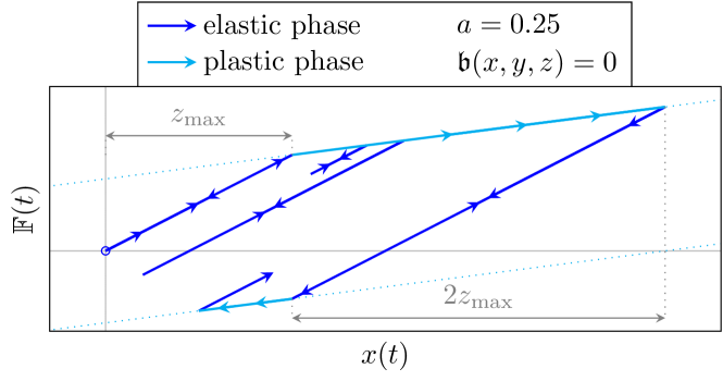
(b) Archetypal evolution of $\mathbb{F}(t)$ and $x(t)$ when $\mathfrak{b}=0$.

Figure A1: Description of the kinematic hardening bilinear elastoplastic model.(a) In the rheological model, $x(t)$ is the total displacement, that is the sum of the elastic $z(t)$ and plastic $\Delta(t)$ ones. The friction component prevents the elastic line from exceeding yield strength $S_{\text{y}}$. The damping term $\mathfrak{b}$ resists the total velocity $y$. (b) For the archetypal evolution of $\mathbb{F}(t)$ and $x(t)$ when $\mathfrak{b}=0$, starting from a neutral position, the behaviour starts being elastic (first elastic phase). Once $x$ exceeds $z_{\text{max}}$ with a positive velocity $y$, $z$ is frozen and $y$ becomes the rate of change of the plastic displacement $\Delta$ (plastic phase). Then, when the velocity becomes negative, $\Delta$ is frozen and $y$ becomes the rate of change of the elastic displacement (second elastic phase).

The other forces $f$ are of the form $\mathfrak{b}(x,y)+\sigma\xi$, where $\mathfrak{b}:\mathbb{R}^{2}\to\mathbb{R}$ is a function that describes the deterministic forces experienced by the oscillator and $\sigma({\color[rgb]{0,0,0}})$ is a positive transient time-dependent function, i.e. vanishing outside of a finite time interval that modulates a Gaussian noise $\xi$, which can be white or coloured. An important example for $\mathfrak{b}$ is when it represents a damping force of the form $\mathfrak{b}(x,y)=-\gamma y$ and $\gamma>0$ is a damping coefficient.

Below, we derive the effective parameters and the corresponding nondimensional system. The parameters $m,k$, and $\mathfrak{s}$ are expressed in kg, kg $\textup{s}^{-2}$ and kg m $\textup{s}^{-3/2}$, respectively. We can introduce the characteristic time and space length, $\tau_{c}\triangleq\sqrt{mk^{-1}}$ and $\ell\triangleq\mathfrak{s}m^{-1}\tau_{c}^{3/2}$. We thus introduce the nondimensional variables

$$t\triangleq\tau\tau_{c}^{-1},\>\>X(t)\triangleq\ell^{-1}x(\tau_{c}t),\>\>Z(t)\triangleq\ell^{-1}z(\tau_{c}t),\mbox{ and }Y(t)\triangleq\ell^{-1}\tau_{c}y(\tau_{c}t).$$

Therefore, we can recast Equation (1) into the nondimensional form

$$\operatorname{d}\!Y/\operatorname{d}\!t+a\hat{k}X+(1-a)\hat{k}Z=\hat{\mathfrak{b}}(X,Y)+\hat{\sigma}\hat{\xi}$$ (2)

where $\hat{k}\triangleq km^{-1}\tau_{c}^{2},\>\hat{\mathfrak{b}}(X,Y)\triangleq\tau_{c}m^{-1}\mathfrak{b}(\ell X,\ell\tau_{c}^{-1}Y),$ and the elastic bound for $Z$ is $\hat{z}_{\textup{max}}\triangleq\ell^{-1}z_{\textup{max}}$. We define the normalization of $\sigma$ as $\hat{\sigma}({\color[rgb]{0,0,0}})\triangleq\sigma({\color[rgb]{0,0,0}})/\mathfrak{s}$, with the noise strength defined as $\mathfrak{s}\triangleq\max\limits_{[0,\infty)}|\sigma|$. Below, we will drop the hats for notational simplicity and proceed with the nondimensional system (2) unless stated otherwise.

2.2 Random forces

Comments on the types of noise $\sigma({\color[rgb]{0,0,0}})$ for practical purposes

A common example used in the earthquake literature [26] for the function $\sigma(\cdot)$ is

$$\sigma(t)=a\,t^{b}e^{-ct},\>\>t\geq 0.$$ (3)

The specific parameters $a,b,c$ can be chosen to obtain a best fit between modulation function and real seismic signal, as shown in [27]. The coloured noise component $\xi$ is characterized by its PSD. In practice, it is possible to extract an empirical PSD from a given data of a real seismic signal [28]. However, this goes beyond the scope of the paper. Instead, we will directly consider coloured noise arising from two general classes of PSDs.

Ornstein-Ulhenbeck processes

From a modeling point of view, using white noise excitations can only be realistic for a very restricted class of seismic applications. To meet the need for more advanced modeling, a natural generalization consists of considering coloured noise, which we model by a class of zero-mean stationary Gaussian processes. The latter can be represented by sums of Ornstein-Uhlenbeck (OU) processes. For the purpose of implementing our hybrid method, we will further require the limiting distribution (as $\varepsilon\rightarrow 0$) of the coloured noise to be that of a white noise. In particular, given $\varepsilon>0$, we will consider noise of the form $\xi^{\varepsilon}=\boldsymbol{r}\cdot\eta^{\varepsilon}/\varepsilon$, with $d\geq 1$, $\boldsymbol{r}=(r_{1},\cdots,r_{d})\in\mathbb{R}^{d}$ and $\eta^{\varepsilon}\in\mathbb{R}^{d}$ is an OU process, i.e. satisfying

$${\rm d}\eta^{\varepsilon}=-\frac{A}{\varepsilon^{2}}\eta^{\varepsilon}{\rm d}t+\frac{K}{\varepsilon}{\rm d}W_{t}$$ (4)

where $A\in\mathbb{R}^{d\times d}$ has eigenvalues with positive real parts, $K\in\mathbb{R}^{d\times d^{\prime}}$, and $W\in\mathbb{R}^{d^{\prime}}$ is a multidimensional standard Brownian motion. In this way, the unique stationary probability measure of $\eta^{\varepsilon}$ is given by a multivariate centered Gaussian distribution with the following covariance matrix

$$C(A,K)\triangleq\int_{0}^{\infty}e^{-As}KK^{T}e^{-A^{T}s}\textup{d}s.$$ (5)

The parameter $\varepsilon$ allows us to adjust the level of autocorrelation in the noise. Using the process $\xi^{\varepsilon}$ above, we can construct two types of real-valued noise depending on the parameter $\varepsilon$ whose PSD are of the form $S^{\varepsilon}(\omega)=S(\varepsilon^{2}\omega)$. We distinguish two cases where the matrices $A,K$ and $\boldsymbol{r}$ have different structures: either $d=q$ or $d=2q$ for $q\geq 1$. For the first type, we consider a sum of centered Lorentzians

$$S(\omega)=\sum\limits_{k=1}^{q}\frac{r_{k}^{2}}{1+\omega^{2}/\lambda_{k}^{2}},$$ (6)

where $\lambda_{1},\dots,\lambda_{q}\in\mathbb{R}$ are constants. Here $S^{\varepsilon}({\color[rgb]{0,0,0}})$ is the PSD of $\xi^{\varepsilon}=\boldsymbol{r}\cdot\eta^{\varepsilon}/\varepsilon$, $\eta^{\varepsilon}$ is the solution of (4) with $d=d^{\prime}=q$ and $A=K=\textup{diag}(\lambda_{1},\cdots,\lambda_{q})$.

For the second type, we consider a sum of uncentered Lorentzian

$$S(\omega)=\frac{1}{2}\left(\sum\limits_{k=1}^{q}\frac{r_{k}^{2}}{1+(\omega-\omega_{k})^{2}/\lambda_{k}^{2}}+\sum\limits_{k=1}^{q}\frac{r_{k}^{2}}{1+(\omega+\omega_{k})^{2}/\lambda_{k}^{2}}\right),$$ (7)

where $\boldsymbol{r}=(r_{1},0,\cdots,r_{q},0)\in\mathbb{R}^{2q}$ and $\lambda_{1},\dots,\lambda_{q},\omega_{1},\dots,\omega_{q}\in\mathbb{R}$ are constant. Here $S^{\varepsilon}({\color[rgb]{0,0,0}})$ is the PSD of $\xi^{\varepsilon}=\boldsymbol{r}\cdot\eta^{\varepsilon}/\varepsilon$, $\eta^{\varepsilon}$ is solution of (4) with $d=d^{\prime}=2q$ and

$$A=\oplus_{k=1}^{q}\begin{pmatrix}\lambda_{k}&-\omega_{k}\\ \omega_{k}&\lambda_{k}\end{pmatrix},\quad K=\oplus_{k=1}^{q}\begin{pmatrix}\lambda_{k}&0\\ 0&\lambda_{k}\end{pmatrix},$$

where the notation $\oplus$ is the direct sum of matrices, i.e. $A,K\in\mathbb{R}^{2q\times 2q}$. We note that in both cases when $\varepsilon\downarrow 0$, $S^{\varepsilon}$ goes to a constant, that is the PSD of white noise, precisely $\xi^{0}=\boldsymbol{r}\cdot A^{-1}K\operatorname{d}\!W/\operatorname{d}\!t=\boldsymbol{r}\cdot\operatorname{d}\!W/\operatorname{d}\!t$ for the first case and $\xi^{0}=\boldsymbol{r}\cdot A^{-1}K\operatorname{d}\!W/\operatorname{d}\!t$ for the second case. This can also be seen intuitively by writing Equation (4) as $\varepsilon^{2}\left(\operatorname{d}\!\eta^{\varepsilon}/\varepsilon\right)=-A\eta^{\varepsilon}\operatorname{d}\!t+K\operatorname{d}\!W_{t}$ and neglecting the left hand side when $\varepsilon$ is small. In the second case, we assume that

$$\sum_{k=1}^{q}r_{k}^{2}=1\>\mbox{ and }\>\sum_{k=1}^{q}\frac{r_{k}^{2}}{1+\omega_{k}^{2}/\lambda_{k}^{2}}=1.$$

Hence, in both cases, $\xi^{0}$ has the same law as $\operatorname{d}\!W/\operatorname{d}\!t$.

2.3 Formulation of kinematic hardening models using stochastic variational inequalities

Inspired by [29], we adopt a mathematical formulation of the models as described in the previous section by representing them with variational inequalities. To describe the dynamics of the kinematic hardening models shown in (1) and driven by the noise $\xi^{\varepsilon}$, we consider the $\mathbb{R}^{3}$ valued process $\{(X^{\varepsilon}(s),Y^{\varepsilon}(s),Z^{\varepsilon}(s)),\>s\geq t\}$ which solves the variational inequality: for a.e. $s>t$,

$$\begin{cases}&\dot{X}^{\varepsilon}(s)=Y^{\varepsilon}(s),\\ &\dot{Y}^{\varepsilon}(s)=\mathfrak{b}(X^{\varepsilon}(s),Y^{\varepsilon}(s))-akX^{\varepsilon}(s)-(1-a)kZ^{\varepsilon}(s)+\sigma(s)\xi^{\varepsilon}(s),\\ &|Z^{\varepsilon}(s)|\leq z_{\textup{max}},\>\forall\varphi\in[-z_{\textup{max}},z_{\textup{max}}],\>(\dot{Z}^{\varepsilon}(s)-Y^{\varepsilon}(s))(\varphi-Z^{\varepsilon}(s))\geq 0,\end{cases} \mathcal{SVI}$$ (9-)

with the initial state $(X^{\varepsilon}(t),Y^{\varepsilon}(t),Z^{\varepsilon}(t))=(x,y,z)\in\mathbb{R}^{2}\times[-z_{\textup{max}},z_{\textup{max}}]$. The problem is well-posed [30] in both cases $\varepsilon>0$ and $\varepsilon=0$.

2.4 Risk of failure

The risk of failure problem consists of finding the probability that, either over a certain interval of time $[0,T]$ or at a given time $T$, the state variable $(x,y,z)\in\mathbb{R}^{2}\times[-z_{\textup{max}},z_{\textup{max}}]$ reaches a given domain of failure, say $D_{\text{f}}\subset\mathbb{R}^{2}\times[-z_{\textup{max}},z_{\textup{max}}]$. In this paper, both types of failures will be considered:

• the ultimate limit state (ULS) probability can be expressed as the probability that the total deformation reaches a threshold $X_{\rm f}$ at any time over a finite time period $[0,T]$. Given that the system is in the state $(x_{0},y_{0},z_{0})$ at $t=0$, this probability is given by:

  $$P_{1}^{\varepsilon}=\mathbb{P}\left(\max_{t\in[0,T]}{{|X^{\varepsilon}(t)|}}\geq X_{\rm f}\>\middle|\>\big{(}X^{\varepsilon}(0),Y^{\varepsilon}(0),Z^{\varepsilon}(0)\big{)}=(x_{0},y_{0},z_{0})\right). \mathbf{ULS}$$ (10-)

  For this quantity, $D_{\rm f}=\left\{(x,y,z),|x|\geq X_{\rm f}\right\}$.

• the serviceability limit state (SLS) probability can be expressed as the probability that the plastic deformation exceeds a threshold $\Delta_{\rm f}$ at the final time $T$. Given that the system is in the state $(x_{0},y_{0},z_{0})$ at $t=0$, this probability is given by:

  $$P_{2}^{\varepsilon}=\mathbb{P}\left({|X^{\varepsilon}(T)-Z^{\varepsilon}(T)|}\geq\Delta_{\text{f}}\>\middle|\>\big{(}X^{\varepsilon}(0),Y^{\varepsilon}(0),Z^{\varepsilon}(0)\big{)}=(x_{0},y_{0},z_{0})\right). \mathbf{SLS}$$ (11-)

  For this quantity, $D_{\rm f}=\left\{(x,y,z),|x-z|\geq\Delta_{\rm f}\right\}$.

Remark 1.

The KBEs related to the risk of failure for the white noise $(\varepsilon=0)$ driven kinematic hardening models are non-standard boundary value problems. For this type of non-standard PDEs where the value of the solution on the boundary depends on the values of the solution inside the domain, only partial existence and uniqueness results are available, mainly for the case where $a=0$ [31]. This is because standard PDE theory techniques do not apply due to the challenging non-standard boundary conditions and the degeneracy of the differential operators involved. Therefore, we adopt the same philosophy as [32] who used numerical techniques. By performing careful convergence tests, their results are highly suggestive of the existence of solutions. We also have performed convergence tests (on sequences of grids with increasing resolution) and all of our results are suggestive that the continuous problem has a solution.

3 Hybrid method combining PDEs and MC for the coloured noise system statistics

It is possible to relate the threshold-crossing probabilities $P_{1}^{0}$ and $P_{2}^{0}$ of the white noise-driven system to the solution of parabolic PDEs with non-standard boundary conditions in the same spirit as [32]. In the first part, we provide a formal presentation of these PDEs. In the second part, we present our hybrid approach which combines the solution of the PDE with our control variate Monte Carlo estimator.

3.1 PDEs for $P_{1}^{0}$ and $P_{2}^{0}$ of the white noise driven system

Fix $T>0$. For $P_{1}^{0}$, we define

$$D_{1}\triangleq(-X_{f},X_{f})\times(-\infty,\infty)\times(-z_{\textup{max}},z_{\textup{max}})\>\>\mbox{ and }\>\>D^{\pm}_{1}\triangleq(-X_{f},X_{f})\times(-\infty,\infty)\times\{\pm z_{\textup{max}}\}.$$

For $P_{2}^{0}$, we define

$$D_{2}\triangleq(-\infty,\infty)\times(-\infty,\infty)\times(-z_{\textup{max}},z_{\textup{max}})\>\>\mbox{ and }\>\>D^{\pm}_{2}\triangleq(-\infty,\infty)\times(-\infty,\infty)\times\{\pm z_{\textup{max}}\}.$$

We introduce the notation $\mathcal{C}_{t,x,z}^{1}\mathcal{C}_{y}^{2}$ for the set of functions continuously differentiable with respect to (w.r.t.) the variables $x,z,t$, and twice continuously differentiable w.r.t. the variable $y$. Below, we use the notation $\mathbf{B}(x,y,z)=\mathfrak{b}(x,y)-kax-k(1-a)z$. Using Ito’s lemma, we can derive the generator of $(X^{0},Y^{0},Z^{0})$, the solution of (9-$\mathcal{SVI}$) driven by the modulated transient white noise $\sigma(t)\xi^{0}(t)$, which in law is the same as $\sigma(t)\operatorname{d}\!W(t)/\operatorname{d}\!t$. Since $\sigma(.)$ is time-dependent, the generator is also time-dependent. It is defined for any function $\varphi\in\mathcal{C}_{t,x,z}^{1}\mathcal{C}_{y}^{2}$ as follows

$$\lim\limits_{h\to 0}\frac{\mathbb{E}\varphi(X^{0}(t+h),Y^{0}(t+h),Z^{0}(t+h))-\varphi(x,y,z)}{h}$$

$$=\left\{\begin{array}[]{ll}L(t)\varphi(x,y,z),&|z|<z_{\textup{max}},\>x,y\in(-\infty,\infty)\\ L_{\pm}(t)\varphi(x,y,\pm z_{\textup{max}}),&z=\pm z_{\textup{max}},\>x,y\in(-\infty,\infty),\end{array}\right.$$

where for any test function $\varphi$

$$L(t)\varphi=\frac{\sigma^{2}(t)}{2}\varphi_{yy}+\mathbf{B}(x,y,z)\varphi_{y}+y\varphi_{x}+y\varphi_{z},$$

$$L^{+}(t)\varphi=\frac{\sigma^{2}(t)}{2}\varphi_{yy}+\mathbf{B}(x,y,z_{\textup{max}})\varphi_{y}+y\varphi_{x}+\min(y,0)\varphi_{z},$$

and

$$L^{-}(t)\varphi=\frac{\sigma^{2}(t)}{2}\varphi_{yy}+\mathbf{B}(x,y,-z_{\textup{max}})\varphi_{y}+y\varphi_{x}+\max(y,0)\varphi_{z}.$$

Here the notation $\varphi_{x}$ stands for the partial derivative of $\varphi$ w.r.t. $x$, etc.

3.1.1 PDE problem for $P_{1}^{0}$

Consider a function $v\in\mathcal{C}_{t,x,z}^{1}\mathcal{C}_{y}^{2}$ that satisfies the following PDE,

$$\begin{cases}&v_{t}+L(t)v=0\;{\rm on}\;D_{1}\times[0,T),\\ &v_{t}+L^{\pm}(t)v=0\;{\rm on}\;D_{1}^{\pm}\times[0,T),\\ &v(\pm X_{f},y,z,t)=1\;{\rm on}\;(-\infty,\infty)\times(-z_{\rm max},z_{\rm max})\times[0,T),\\ &v(x,y,z,T)=0\;{\rm on}\;D_{1}.\end{cases}$$ (12)

Then $v(x,y,z,t)=\mathbb{P}[\tau_{t}\leq T|(X^{0}_{t},Y^{0}_{t},Z^{0}_{t})=(x,y,z)]$ where $\tau_{t}=\inf\{s\geq t,\>|X^{0}_{s}|=X_{\rm f}\}$. Hence, $v(x,y,z,0)=P_{1}^{0}$.

3.1.2 PDE problem for $P_{2}^{0}$

Consider a function $w\in\mathcal{C}_{t,x,z}^{1}\mathcal{C}_{y}^{2}$. Assume $w$ satisfies

$$\begin{cases}&w_{t}+L(t)w=0\>\mbox{ in }\>D_{2}\times[0,T),\\ &w_{t}+L^{\pm}(t)w=0\>\mbox{ in }\>D^{\pm}_{2}\times[0,T),\\ &w(T)=f\>\mbox{ in }\>D_{2}\cup D_{2}^{-}\cup D_{2}^{+}.\end{cases}$$ (13)

Then $w(x,y,z,t)=\mathbb{E}[f(X^{0}(T),Y^{0}(T),Z^{0}(T))|(X^{0}(0),Y^{0}(0),Z^{0}(0))=(x,y,z)]$. As a consequence, if $f(x,y,z)=\mathbf{1}_{\{|x-z|\geq\Delta_{\rm f}\}}$ then $w(x,y,z,0)=P_{2}^{0}$.

3.2 Control variate MC estimator for $P_{1}^{\varepsilon}$ and $P_{2}^{\varepsilon}$ of the coloured noise driven system

In this section, we present our MC estimator for the computation of the threshold crossing probabilities $P_{1}^{\varepsilon}$ and $P_{2}^{\varepsilon}$. We explain how it fits into the formalism and the convergence results of [33].

The probabilities $P_{1}^{\varepsilon}$ and $P_{2}^{\varepsilon}$ are similar to quantities of the form

$$I^{\varepsilon}\triangleq\mathbb{E}(F\{(X^{\varepsilon}(t),Y^{\varepsilon}(t),Z^{\varepsilon}(t)),0\leq t\leq T\})$$

where $F$ is a real-valued function on the space of continuous functions on $[0,T]$. For $P_{1}^{\varepsilon}$ and $P_{2}^{\varepsilon}$, the underlying functions are respectively

$$F_{1}(x,y,z)=\mathbf{1}_{\left\{\max\limits_{t\in[0,T]}|x(s)|\geq X_{\rm f}\right\}}\>\mbox{ and }\>F_{2}(x,y,z)=\mathbf{1}_{\{|x(T)-z(T)|\geq\Delta_{\rm f}\}}.$$

Other possible examples (not treated in this work) include functions of the form

$$F(x,y,z)=f(x(T),y(T),z(T))+\int_{0}^{T}g(x(s),y(s),z(s))\textup{d}s$$

where $f,g$ are real valued functions on $\mathbb{R}^{3}$.

Our estimator is built using a coupling approach as follows. Use the notation $U^{0}\triangleq(X^{0},Y^{0},Z^{0})$ and $U^{\varepsilon}\triangleq(X^{\varepsilon},Y^{\varepsilon},Z^{\varepsilon})$, where $\varepsilon>0$. Here $U^{0}$ and $U^{\varepsilon}$ satisfy (9-$\mathcal{SVI}$) where the random forces are given by $\xi^{0}$ and $\xi^{\varepsilon}$, respectively. Most importantly, $U^{0}$ and the coloured noise $\xi^{\varepsilon}$ are driven by the same Wiener process $W$. See the driving noise in Equation (4). In this way, $U^{0}$ and $U^{\varepsilon}$ are correlated. We will use the notation $U^{\varepsilon}(W)$ and $U^{0}(W)$ to state that they are indeed driven by the same randomness. For $\mathbb{E}(F(U^{\varepsilon}))$, the simple MC estimator by control variate is defined as

$$\hat{J}_{N}^{\varepsilon}\triangleq\mathbb{E}(F(U^{0}))+\frac{1}{N}\sum_{k=1}^{N}F(U^{\varepsilon}(W^{k}))-F(U^{0}(W^{k}))$$ (14)

where $W^{k},k=1\dots N$ are $N$ independent and identically distributed Wiener processes. The asymptotic distribution of the estimator is normal with asymptotic variance $\sigma_{J}^{\varepsilon}=\textup{var}\left(F(U^{\varepsilon})-F(U^{0})\right)$.

We also consider the practical optimal MC estimator by control variate defined as

$$\hat{K}_{N}^{\varepsilon}\triangleq\hat{\rho}_{N}^{\epsilon}\mathbb{E}(F(U^{0}))+\frac{1}{N}\sum_{k=1}^{N}F(U^{\varepsilon}(W^{k}))-\hat{\lambda}_{N}^{\epsilon}F(U^{0}(W^{k})),$$ (15)

where

$$\hat{\lambda}_{N}^{\epsilon}\triangleq\frac{\sum\limits_{k=1}^{N}(F(U^{\varepsilon}(W^{k})-\hat{E}_{MC}^{N,\varepsilon})(F(U^{0}(W^{k})-\hat{I}_{N}^{0})}{\sum\limits_{k=1}^{N}(F(U^{0}(W^{k})-\hat{I}_{N}^{0})^{2}}$$

with

$$\hat{I}_{N}^{0}\triangleq\frac{1}{N}\sum\limits_{k=1}^{N}F(U^{0}(W^{k})\>\mbox{ and }\>\hat{I}_{N}^{\varepsilon}\triangleq\frac{1}{N}\sum\limits_{k=1}^{N}F(U^{\varepsilon}(W^{k}).$$

This estimator contrasts with the theoretical optimal control variate estimator as we replace the optimal coefficient $\hat{\lambda}_{N}^{\epsilon}$ with the empirical one $\lambda^{\epsilon}\triangleq\mathrm{cov}(F(U^{\varepsilon}),F(U^{0}))/\mathrm{var}(F(U^{0}))$. Here, the asymptotic distribution is normal with asymptotic variance $\sigma_{K}^{\varepsilon}=\textup{var}\left(F(U^{\varepsilon})-\lambda^{\epsilon}F(U^{0})\right)$.

In comparison, the standard Monte Carlo estimator

$$\hat{I}_{N}^{\varepsilon}\triangleq\frac{1}{N}\sum_{k=1}^{N}F(U^{\varepsilon}(W^{k}))$$ (16)

is asymptotically normal but with asymptotic variance $\sigma_{I}^{\varepsilon}=\textup{var}\left(F(U^{\varepsilon})\right)$.

Let us remark that our Equation (9-$\mathcal{SVI}$) is contained in the class of variational inequalities that appear in Equation (2.31) of [33]. When $\sigma(\cdot)\equiv\sigma_{0}$ is constant, Proposition 5.2 of [33] implies the convergence in probability of the continuous process $U^{\varepsilon}-U^{0}$ to $0$. This property is also valid when $\sigma(\cdot)$ is continuous on $[0,T]$ which is the case of our present paper. Allowing for a few minor modifications, the proof is the same as in the case in which $\sigma(\cdot)$ is constant. As a consequence, when $F(\cdot)$ is bounded and continuous, $\sigma_{J}^{\varepsilon}$ vanishes as $\varepsilon\to 0$. On the other hand, $\sigma_{I}^{\varepsilon}\to\textup{var}\left(F(U^{0})\right)$, thus making the variance reduction possible when $\varepsilon$ is small enough. The estimator $\hat{K}_{N}^{\varepsilon}$ inherits this property, as it is optimized so that its variance is always smaller than those of the estimators $\hat{I}_{N}^{\varepsilon}$ and $\hat{J}_{N}^{\varepsilon}$. In fact, it is also possible to characterize the rate of variance reduction when $F(\cdot)$ has a particular structure such as $F(x,y,z)=f(x(T),y(T),z(T))$ where $f$ is smooth with bounded derivative. Indeed as shown in Lemma 6.1 of [33], both variances $\sigma_{J}^{\varepsilon}$ and $\sigma_{K}^{\varepsilon}$ are of the order $O(\varepsilon)$ when $\varepsilon\to 0$. Although $F_{1}$ and $F_{2}$ do not exactly fall into the class of continuous functions on the path space, our estimator for $P_{1}^{\varepsilon}$ and $P_{2}^{\varepsilon}$ appears to be highly efficient in this context. We will illustrate this using the numerical results shown below.

4 Numerical simulations

4.1 Finite difference method for the PDEs

Here, we present the finite difference method discretization of the PDE associated with $P_{1}^{0}$. The corresponding discretization for the PDE associated with $P_{2}^{0}$ follows similarly with appropriate modifications.

For the computation of $P_{1}^{0}$, we need to truncate $D_{1}$ and $D^{\pm}_{1}$ and add artificial boundary conditions at $y=\pm\bar{y}$ with $\bar{y}>0$. Let $\mathcal{R}\triangleq[-X_{f},X_{f}]\times(-\bar{y},\bar{y})\times[-\bar{z},\bar{z}]$ and define

$$D_{1,\mathcal{R}}\triangleq D_{1}\cap\mathcal{R}=(-X_{f},X_{f})\times(-\bar{y},\bar{y})\times(-\bar{z},\bar{z}),$$

$$D_{1,\mathcal{R}}^{\pm}\triangleq D^{\pm}_{1}\cap\mathcal{R}=(-X_{f},X_{f})\times(-\bar{y},\bar{y})\times\{\pm\bar{z}\},$$

$$\Gamma^{X_{f}}_{1}\triangleq\{\pm X_{f}\}\times[-\bar{y},\bar{y}]\times[-\bar{z},\bar{z}],\>\mbox{ and }\Gamma^{\bar{y}}_{1}\triangleq(-X_{f},X_{f})\times\{-\bar{y},\bar{y}\}\times[-\bar{z},\bar{z}].$$

The value of $\bar{y}$ is chosen sufficiently large such that the probability of the underlying process outside $D_{1,\mathcal{R}}$ is sufficiently small that it does not affect the solution at the desired accuracy. We impose artificial reflecting boundary conditions to each of the four equations in (12). Thus we consider the problem of finding $v$ satisfying

$$\begin{cases}v_{t}+L(t)v=0,&\>\mbox{on}\>D_{1,\mathcal{R}}\times[0,T),\\ v_{t}+L^{\pm}(t)v=0,&\>\mbox{on}\>D_{1,\mathcal{R}}^{\pm}\times[0,T),\\ v_{y}=0,&\>\mbox{on}\>\Gamma^{\bar{y}}_{1}\times[0,T),\\ v=1,&\>\mbox{on}\>\Gamma^{X_{f}}_{1}\times[0,T),\\ v(T)=0,&\>\mbox{on}\>D_{1,\mathcal{R}},\end{cases}$$ (17)

where $L(t)$ and $L^{\pm}(t)$ are defined in Section 3.1, and

$$L^{\pm\bar{x}}(t)\varphi=\frac{\sigma^{2}(t)}{2}\varphi_{yy}+\mathbf{B}(\pm\bar{x},y,z)\varphi_{y}\pm\min(\pm y,0)\varphi_{x}+y\varphi_{z},$$

$$L^{\pm\bar{x},+}(t)\varphi=\frac{\sigma^{2}(t)}{2}\varphi_{yy}+\mathbf{B}(\pm\bar{x},y,\bar{z})\varphi_{y}\pm\min(\pm y,0)\varphi_{x}+\min(y,0)\varphi_{z},$$

$$L^{\pm\bar{x},-}(t)\varphi=\frac{\sigma^{2}(t)}{2}\varphi_{yy}+\mathbf{B}(\pm\bar{x},y,-\bar{z})\varphi_{y}\pm\min(\pm y,0)\varphi_{x}+\max(y,0)\varphi_{z}.$$

Here we recall the elementary identity $-\min(-y,0)=\max(y,0)$. The truncation of the PDE associated with $P_{2}^{0}$ follows similarly but with an additional artificial reflecting boundary condition at $x=\pm\bar{x}$, for sufficiently large $\bar{x}$. Let $\mathcal{S}\triangleq(-\bar{x},\bar{x})\times(-\bar{y},\bar{y})\times[-\bar{z},\bar{z}]$ and similarly define

$$D_{2,\mathcal{S}}\triangleq D_{2}\cap\mathcal{S},\>\>D_{2,\mathcal{S}}^{\pm}\triangleq D^{\pm}_{2}\cap\mathcal{S},\>\>\mathrm{and}\>\>\Gamma^{\bar{y}}_{2}\triangleq[-\bar{x},\bar{x}]\times\{\pm\bar{y}\}\times[-\bar{z},\bar{z}].$$

For the purpose of the artificial reflecting boundary at $\pm\bar{x}$, we define two additional domains

$$\Gamma^{\pm\bar{x}}_{2}\triangleq\{\pm\bar{x}\}\times(-\bar{y},\bar{y})\times(-\bar{z},\bar{z}),\>\>\mathrm{and}\>\>\Gamma^{\pm\bar{x},\pm}_{2}\triangleq\{\pm\bar{x}\}\times(-\bar{y},\bar{y})\times\{\pm\bar{z}\}.$$

The solution of the PDE now corresponds to solving for $w$ satisfying the set of equations as above but with the last two equations replaced by

$$\begin{cases}w_{t}+L^{\pm\bar{x}}(t)w=0,&\>\mbox{on}\>\Gamma^{\pm\bar{x}}_{2}\times[0,T),\\ w_{t}+L^{\pm\bar{x},\pm}(t)w=0,&\>\mbox{on}\>\Gamma^{\pm\bar{x},\pm}_{2}\times[0,T),\\ w(T)=f,&\>\mbox{on}\>D_{2,\mathcal{S}}.\end{cases}$$ (18)

along with the appropriate changes made corresponding to the three equations (13).

To numerically approximate the solutions of the equations (17) and (18), we employ a finite difference scheme. Let $\tilde{I},\tilde{J},\tilde{K}$ be integers and define $I=2\tilde{I}+1$, $J=2\tilde{J}+1$, $K=2\tilde{K}+1$. We build our approximation on the following three-dimensional finite difference grid,

$$\mathcal{G}\triangleq\{(x_{i},y_{j},z_{k})=(-\bar{x}+(i-1)\delta x,-\bar{y}+(j-1)\delta y,-\bar{z}+(k-1)\delta z),\>1\leq i\leq I,1\leq j\leq J,1\leq k\leq K\}$$

where $\delta x\triangleq\bar{x}/\tilde{I}$, $\delta y\triangleq\bar{y}/\tilde{J}$ $\delta z\triangleq\bar{z}/\tilde{K}$, and hence there are $P\triangleq IJK$ points in the grid. We then, denote $t_{n}\triangleq n\delta t$ with $\delta t=T/N_{T}$, where $N_{T}$ is the number of time steps. We use the notation $v_{i,j,k}^{n}$ for the approximation of $v(x_{i},y_{j},z_{k},t_{n})$, $\mathbf{v}^{n}$ for the vector of $P$ unknown when $n$ is fixed, and $f_{i,j,k}$, $\sigma_{n}$, $B_{i,j,k}$ for $f(x_{i},y_{j},z_{k})$, $\sigma(t_{n})$, $B(x_{i},y_{j},z_{k})$, respectively. The computation of $\mathbf{v}^{n}$ is obtained via a Crank-Nicolson finite difference scheme in space. We use the following short-hand notation for centered finite differences of orders 2 and 1,

$$\begin{pmatrix}{\partial_{x}^{2}w}\end{pmatrix}_{i,j,k}\triangleq\frac{w_{i+1,j,k}-2w_{i,j,k}+w_{i-1,j,k}}{\delta x^{2}},\>\mbox{ and }\>\begin{pmatrix}{\partial_{x}w}\end{pmatrix}_{i,j,k}\triangleq\frac{w_{i+1,j,k}-w_{i-1,j,k}}{2\delta x},$$

and forward and backward finite differences of order 1

$$\begin{pmatrix}{\partial_{x}^{f}w}\end{pmatrix}_{i,j,k}\triangleq\frac{w_{i+1,j,k}-w_{i,j,k}}{\delta x}\>\mbox{ and }\>\begin{pmatrix}{\partial_{x}^{b}w}\end{pmatrix}_{i,j,k}\triangleq\frac{w_{i,j,k}-w_{i-1,j,k}}{\delta x}.$$

Moreover, we also denote for any function of $y$, $c(y)$,

$$\begin{pmatrix}{c(y)\hat{\partial}_{x}w}\end{pmatrix}_{i,j,k}\triangleq\min(0,c(y_{j}))\begin{pmatrix}{\partial_{x}^{b}w}\end{pmatrix}_{i,j,k}+\max(0,c(y_{j}))\begin{pmatrix}{\partial_{x}^{f}w}\end{pmatrix}_{i,j,k}.$$

The centered, forward, and backward finite differences w.r.t. $y$ and $z$ are defined similarly. At each time step $n\in\{0,...,N_{T}-1\}$ (decreasing in $n$), $\mathbf{v}^{n+1}$ is known and we solve for $\mathbf{v}^{n}$. This leads to the following set of $P$ linear equations:

• when $1\leq i\leq I,2\leq j\leq J-1,1\leq k\leq K,$

  $$\frac{v_{i,j,k}^{n+1}-v_{i,j,k}^{n}}{\delta t}+\frac{1}{2}\left(\begin{pmatrix}{L^{n+1}v^{n+1}}\end{pmatrix}_{i,j,k}+\begin{pmatrix}{L^{n}v^{n}}\end{pmatrix}_{i,j,k}\right)=0,$$

• when $1\leq i\leq I,j=\{1,J\},1\leq k\leq K,$

  $$\begin{pmatrix}{\partial_{y}^{f}w^{n}}\end{pmatrix}_{i,1,k}=0\>\mbox{ and }\>\begin{pmatrix}{\partial_{y}^{b}w^{n}}\end{pmatrix}_{i,J,k}=0.$$

Here when $2\leq i\leq I-1,\>2\leq j\leq J-1,\>2\leq k\leq K-1,$

$$\begin{pmatrix}{L^{n}w^{n}}\end{pmatrix}_{i,j,k}\triangleq\frac{\sigma_{n}^{2}}{2}\begin{pmatrix}{\partial_{y}^{2}w^{n}}\end{pmatrix}_{i,j,k}+B_{i,j,k}\begin{pmatrix}{\partial_{y}w^{n}}\end{pmatrix}_{i,j,k}+\begin{pmatrix}{y\hat{\partial}_{x}w^{n}}\end{pmatrix}_{i,j,k}+\begin{pmatrix}{y\hat{\partial}_{z}w^{n}}\end{pmatrix}_{i,j,k}.$$

Otherwise, we modify $(L^{n}w^{n})_{i,j,k}$ at the boundary. The last two terms describe the transport of the underlying process in the directions $x$ and $z$. They contain four terms

$$\min(0,y_{j})\begin{pmatrix}{\partial_{x}^{b}w^{n}}\end{pmatrix}_{i,j,k}+\max(0,y_{j})\begin{pmatrix}{\partial_{x}^{f}w^{n}}\end{pmatrix}_{i,j,k}+\min(0,y_{j})\begin{pmatrix}{\partial_{z}^{b}w^{n}}\end{pmatrix}_{i,j,k}+\max(0,y_{j})\begin{pmatrix}{\partial_{z}^{f}w^{n}}\end{pmatrix}_{i,j,k}.$$

To be consistent with Equations (17) and (18), the outward flux terms are removed from $(L^{n}w^{n})_{i,j,k}$ at the boundary. We explicitly the modify the operator as follows: in all cases $2\leq j\leq J-1$, whenever $i=1$ or $k=1$, the terms to be removed from $(L^{n}w^{n})_{i,j,k}$ are

$$\min(0,y_{j})\begin{pmatrix}{\partial_{x}^{b}w^{n}}\end{pmatrix}_{i,j,k}\>\mbox{ or }\>\min(0,y_{j})\begin{pmatrix}{\partial_{z}^{b}w^{n}}\end{pmatrix}_{i,j,k},\>\textup{respectively}.$$

Similarly, whenever $i=I$ or $k=K$, the terms to be removed from $(L^{n}w^{n})_{i,j,k}$ are

$$\max(0,y_{j})\begin{pmatrix}{\partial_{x}^{f}w^{n}}\end{pmatrix}_{i,j,k}\>\mbox{ or }\>\max(0,y_{j})\begin{pmatrix}{\partial_{z}^{f}w^{n}}\end{pmatrix}_{i,j,k},\>\textup{respectively}.$$

Note that at most two terms can be removed.

4.2 Numerical examples

4.2.1 Numerical Solution of $P_{1}^{0}$ and $P_{2}^{0}$ (white noise driven probabilities)

To obtain solutions of the two PDEs in Section 3.1, we numerically solve the linear systems from Section 4.1 backward in time between the time steps $n=N_{T}$ and $n=0$. In particular, at each time step, we solve the linear systems by the method of Generalized Minimal Residuals with tolerance $=10^{-6}$, and precondition each system with Incomplete LU Factorization. For the discretized PDE corresponding to $P_{1}^{0}$, convergence of the solutions has been obtained with the choice of artificial boundary $\bar{y}=2.5$, space step sizes of $\delta x=\delta z=2^{-9}$, $\delta y=2^{-6}$, and time step sizes of $\delta t=10^{-4}$. Similarly, convergence of solutions can be shown with the same choice of parameters but with $\bar{x}=2.5$ for the discretized PDE corresponding to $P_{2}^{0}$.

Figure A2 presents the results for the probabilities $P_{1}^{0}$ and $P_{2}^{0}$ for a range of threshold values $X_{f}$ and $\Delta_{f}$, represented by the red dots, by the numerical KBE method. For comparison, approximations of the same probabilities $P_{1}^{0}$ and $P_{2}^{0}$, represented by the blue lines, have been computed with the intensive Monte Carlo method with time step $\delta t=10^{-3}$ and $10^{8}$ samples. All results were obtained using the parameters $a=2.84$, $b=2$, and $c=1.25$ for the modulation function (3); these parameters are commonly used, e.g. [34]. In addition, we will take the damping function to be $\mathfrak{b}(x,y)\triangleq-y$. These results highlight an excellent agreement between the two methods.

(a)

(b)

Figure A2: Probabilities $P_{1}^{0}$ (left) and $P_{2}^{0}$ (right) taken from the numerical solution of the PDEs (red dots) and from the Monte Carlo Simulations (blue line).

4.2.2 Estimators and Variance Reduction

In this section, for the coloured-noise-driven system, we estimate the small probability $P^{\epsilon}_{1}$ corresponding to $X_{f}=2$ with the three types of estimators: the standard MC estimator $\hat{I}^{\epsilon}_{N}$ in Equation (16), the simple control variate estimator $\hat{J}^{\epsilon}_{N}$ in Equation (14), and the optimal control variate estimator $\hat{K}^{\epsilon}_{N}$ in Equation (15) using the value $P^{0}_{1}$ obtained from the KBE approach in Section 4.2.1. We consider two types of coloured noise $\xi^{\epsilon}$: the first with PSD of the form Equation (6) at $\lambda=1$ (PSD1), and the second with PSD of the form Equation (7) with $\lambda=\omega=1$ (PSD2), both with $q=1$. We will consider a range of values $\epsilon>0$, which we recall, indicates the level of autocorrelation between the coloured and white noises. At each value $\epsilon$, we run two separate MC simulations at time step $\delta t=10^{-4}$ with $N=10^{5}$ and $N=10^{6}$ samples to compute the estimated value $P^{\epsilon}_{1}$ and the variance $\sigma^{2}$, respectively, of each of the three estimators: $\hat{I}_{N}^{\varepsilon}$ (standard MC), $\hat{J}_{N}^{\varepsilon}$ (simple control variate) and $\hat{K}_{N}^{\varepsilon}$ (practical optimal control variate). The Euler-Maruyama time discretizations of the SVI 9-$\mathcal{SVI}$ and coloured noise dynamics 4 with PSDs of the forms 6 and 7 are given in A.

Figures A3, A3 compares the estimated values for PSD1 and PSD2, respectively. Note that the estimated values of $P^{\epsilon}_{1}$ tend to $P^{0}_{1}$ from the KBE as $\varepsilon$ tends to $0$ as expected from approximation diffusion theory in Section 3.2. Figures A3, A3 presents the corresponding empirical variances of the estimators $\hat{I}_{N}^{\varepsilon},\hat{J}_{N}^{\varepsilon}$ and $\hat{K}_{N}^{\varepsilon}$. Observe that indeed the optimal control variate estimator attains lower variance than both the standard MC and simple control variate estimators. In addition, it provides a robust estimate over the whole range of $\varepsilon$ values. For PSD1 and PSD2, the numerical results shown in Figures A3 and A3 empirically reveal an estimate for the variance bound in the form $O(\varepsilon^{1+\delta})$ with $\delta\approx 1$. This is finer than that predicted by the theory in $O(\varepsilon)$ when $F(x,y,z)=f(x(T),y(T),z(T))$ with $f$ being smooth with bounded derivatives. As shown in Figure A4, in the estimate of $P_{2}^{\varepsilon}$, we observe a behavior similar to what we observe in Figures A3, A3, A3, and A3. However, comparing A3 and A3 with A4 and A4, we empirically see that the $\sigma_{\hat{K}_{N}^{\varepsilon}}^{2}/\varepsilon^{2}$ remains bounded for (10-$\mathbf{ULS}$) but becomes unbounded as $\varepsilon\to 0^{+}$ for (11-$\mathbf{SLS}$).

Figure A3: Monte Carlo estimation of $P^{\epsilon}_{1}$ using $\hat{I}_{N}^{\varepsilon}$ (standard MC), $\hat{J}_{N}^{\varepsilon}$ (simple control variate) and $K_{N}^{\varepsilon}$ (practical optimal control variate). For $\hat{J}_{N}^{\varepsilon}$ and $K_{N}^{\varepsilon}$, the expectation of the control variate $P^{0}_{1}$ is obtained by solving the PDE (12). This is done numerically by finite differences shown in Section 4.1. The driving coloured noise is related to PSD1 for the left column (a)-(b)-(c), and PSD2 for the right column (a’)-(b’)-(c’). The time discretization of the KBEPO dynamics together with the driving noise (coloured or white) is given in (19)-(20)-(21) in the appendix.

Figure A4: Monte Carlo estimation of $P^{\epsilon}_{2}$ using $\hat{I}_{N}^{\varepsilon}$ (standard MC), $\hat{J}_{N}^{\varepsilon}$ (simple control variate) and $K_{N}^{\varepsilon}$ (practical optimal control variate). For $\hat{J}_{N}^{\varepsilon}$ and $K_{N}^{\varepsilon}$, the expectation of the control variate $P^{0}_{2}$ is obtained by solving the PDE (13). This is done numerically by finite differences shown in Section 4.1. The driving coloured noise is related to PSD1 for the left column (a)-(b)-(c), and PSD2 for the right column (a’)-(b’)-(c’). The time discretization of the KBEPO dynamics together with the driving noise (coloured or white) is given in (19)-(20)-(21) in the appendix.

5 Conclusion

We have developed an efficient method for computing probabilities with transient modulated, coloured noise excitation and with target quantities of type (10-$\mathbf{ULS}$) and (11-$\mathbf{SLS}$). These quantities of interest are representative of an important class of problems in earthquake engineering. Our method has been shown to have good accuracy and is more computationally efficient than standard Monte Carlo methods. It also does not make any approximation other than the discretisation of the domain for solving the PDEs, unlike stochastic averaging or other common methods which approximate the process. Previous work was handled on the white noise-driven EPPO [32], which was computationally less challenging because it can be reduced to a 2-dimensional problem. That study also used stationary excitation and only considered (10-$\mathbf{ULS}$) type quantities. Our current method is non-trivial generalization of this approach. We can take into account the K-BEPO, non-stationary coloured noise excitation and (10-$\mathbf{ULS}$),(11-$\mathbf{SLS}$) -type quantities. As mentioned above, these features are essential for engineering fields like earthquake engineering. With this paper, we show that the concept developed in [33, 32] can indeed be used in engineering in more realistic situations and with commonly used models like K-BEPO.

Appendix A Time discretization of the coloured noise and the stochastic variational inequalities

Fix the final time $T>0$, the number of time steps $N_{T}\in\mathbb{N}$, and the number of Monte Carlo samples $N$. Define $\delta t$ such that $T=N_{T}\delta t$. Furthermore, take a sequence of i.i.d. $d^{\prime}$-dimensional Gaussian variables $\{\Delta W_{n}^{k}\sim\mathcal{N}\left(0,I_{d^{\prime}}\right),\>0\leq n\leq N_{T}-1,\>1\leq k\leq N\},$ where $\mathcal{N}(0,\sigma^{2})$ denotes a normal distribution with mean $0$ and variance $\sigma^{2}$. For the $k$-th sample, $1\leq k\leq N$, the discretization of the OU process $\eta^{\varepsilon,k}$ is given by the following:

If $A\in\mathbb{R}^{d\times d},K\in\mathbb{R}^{d\times d^{\prime}}$ in (4) are arbitrary, then

$$\begin{cases}\hat{\eta}_{0}^{\varepsilon,k}&\sim\mathcal{N}\left(0,C(A,K)\right),\\ \hat{\eta}_{n+1}^{\varepsilon,k}&=(I-\frac{\delta t}{\varepsilon^{2}}A)\hat{\eta}_{n}^{\varepsilon,k}+(\frac{\sqrt{\delta t}}{\varepsilon}K)\Delta W_{n}^{k},\>\>0\leq n\leq N_{T}-1,\end{cases}$$ (19)

where $C(A,K)$ is the covariance matrix (5). In particular, we have

• If the PSD of $\eta^{\varepsilon,k}$ takes the form (6) with $q=1$, then $d=d^{\prime}=1$ and

  $$\begin{cases}\hat{\eta}_{0}^{\varepsilon,k}&\sim\mathcal{N}\left(0,\lambda_{1}/2\right),\\ \hat{\eta}_{n+1}^{\varepsilon,k}&=(1-\frac{\delta t}{\varepsilon^{2}}\lambda_{1})\hat{\eta}_{n}^{\varepsilon,k}+(\frac{\sqrt{\delta t}}{\varepsilon}\lambda_{1})\Delta W_{n}^{k},\>\>0\leq n\leq N_{T}-1.\end{cases}$$

• If the PSD of $\eta^{\varepsilon}$ takes the form (7) with $q=1$, then $d=d^{\prime}=2$ and

  $$\begin{cases}(\hat{\eta}_{0}^{\varepsilon,k})_{1}&\sim\mathcal{N}\left(0,\lambda_{1}/2\right),\\ (\hat{\eta}_{0}^{\varepsilon,k})_{2}&\sim\mathcal{N}\left(0,\lambda_{1}/2\right),\\ (\hat{\eta}_{n+1}^{\varepsilon,k})_{1}&=(1-\frac{\delta t}{\varepsilon^{2}}\lambda_{1})(\hat{\eta}_{n}^{\varepsilon,k})_{1}+(\frac{\delta t}{\varepsilon^{2}}\omega_{1})(\hat{\eta}_{n}^{\varepsilon,k})_{2}+(\frac{\sqrt{\delta t}}{\varepsilon}\lambda_{1})(\Delta W_{n}^{k})_{1},\>\>0\leq n\leq N_{T}-1,\\ (\hat{\eta}_{n+1}^{\varepsilon,k})_{2}&=(1-\frac{\delta t}{\varepsilon^{2}}\lambda_{1})(\hat{\eta}_{n}^{\varepsilon,k})_{2}-(\frac{\delta t}{\varepsilon^{2}}\omega_{1})(\hat{\eta}_{n}^{\varepsilon,k})_{1}+(\frac{\sqrt{\delta t}}{\varepsilon}\lambda_{1})(\Delta W_{n}^{k})_{2},\>\>0\leq n\leq N_{T}-1.\end{cases}$$

  where $({\color[rgb]{0,0,0}})_{i}$ denotes the $i$-th component.

For the time discretization of the coupling between the two stochastic variational inequalities, we proceed as follows :

• $\hat{X}_{0}^{\varepsilon,k}=x,\>\hat{Y}_{0}^{\varepsilon,k}=y,\>\hat{Z}_{0}^{\varepsilon,k}=z$ and for $0\leq n\leq N_{T}-1$

  $$\begin{cases}&\hat{X}_{n+1}^{\varepsilon,k}=\hat{X}_{n}^{\varepsilon,k}+\delta t\hat{Y}_{n}^{\varepsilon,k},\\ &\hat{Y}_{n+1}^{\varepsilon,k}=\hat{Y}_{n}^{\varepsilon,k}+\delta t\mathbf{B}(\hat{X}_{n}^{\varepsilon,k},\hat{Y}_{n}^{\varepsilon,k},\hat{Z}_{n}^{\varepsilon,k})+\sigma(n\delta t)\delta t\>r\cdot\hat{\eta}_{n}^{\varepsilon,k}/\varepsilon,\\ &\hat{Z}_{n+1}^{\varepsilon,k}=\textup{proj}_{[-z_{\textup{max}},z_{\textup{max}}]}\left(\hat{Z}_{n}^{\varepsilon,k}+\delta t\hat{Y}_{n}^{\varepsilon,k}\right).\end{cases}$$ (20)

• $\hat{X}_{0}^{0,k}=x,\>\hat{Y}_{0}^{0,k}=y,\>\hat{Z}_{0}^{0,k}=z$ and for $0\leq n\leq N_{T}-1$

  $$\begin{cases}\hat{X}_{n+1}^{0,k}=\hat{X}_{n}^{0,k}+\delta t\hat{Y}_{n}^{0,k},\\ \hat{Y}_{n+1}^{0,k}=\hat{Y}_{n}^{0,k}+\delta t\mathbf{B}(\hat{X}_{n}^{0,k},\hat{Y}_{n}^{0,k},\hat{Z}_{n}^{0,k})+\sigma(n\delta t)\sqrt{\delta t}\>r\cdot A^{-1}K\Delta W_{n}^{k},\\ \hat{Z}_{n+1}^{0,k}=\textup{proj}_{[-z_{\textup{max}},z_{\textup{max}}]}\left(\hat{Z}_{n}^{0,k}+\delta t\hat{Y}_{n}^{0,k}\right).\end{cases}$$ (21)

See [35, p 305-337] for a detailed account of the time-discretization of SDEs.

References

- [1] J. L. Chaboche, K. D. Van, and G. Cordier. Modelization of the strain memory effect on the cyclic hardening of 316 stainless steel. 1979.
- [2] P. Lipinski and M. Berveiller. Elastoplasticity of micro-inhomogeneous metals at large strains. International Journal of Plasticity, 5(2):149–172, 1989.
- [3] J. Dirrenberger, S. Forest, and D. Jeulin. Elastoplasticity of auxetic materials. Computational Materials Science, 64:57–61, 2012.
- [4] R. V. Milligan, W. H. Koo, and T. E. Davidson. The bauschinger effect in a high-strength steel. Journal of Basic Engineering, 88(2):480–488, 1966.
- [5] R. Sowerby, D. K. Uko, and Y. Tomita. A review of certain aspects of the bauschinger effect in metals. Materials Science and Engineering, 41(1):43–58, 1979.
- [6] S. Patinet, A. Barbot, M. Lerbinger, D. Vandembroucq, and A. Lemaître. Origin of the bauschinger effect in amorphous solids. Physical Review Letters, 124(20):205503, 2020.
- [7] G. W. Housner. The behavior of inverted pendulum structures during earthquakes. Bulletin of the seismological society of America, 53(2):403–417, 1963.
- [8] R. D. Campbell, R. P. Kennedy, and R. D. Trasher. Inelastic response of piping systems subjected to in-structure seismic excitation. American Society of Mechanical Engineers. Paper, page 10, 1983.
- [9] F. Touboul, P. Sollogoub, and N. Blay. Seismic behaviour of piping systems with and without defects: experimental and numerical evaluations. Nuclear engineering and design, 192(2-3):243–260, 1999.
- [10] C. Feau, I. Politopoulos, G. S. Kamaris, C. Mathey, T. Chaudat, and G. Nahas. Experimental and numerical investigation of the earthquake response of crane bridges. Engineering Structures, 84:89–101, 2015.
- [11] S. Kasinos, A. Palmeri, and M. Lombardo. Performance-based seismic analysis of light sdof secondary substructures. 2015.
- [12] P. P. Rossi. Importance of isotropic hardening in the modeling of buckling restrained braces. Journal of Structural Engineering, 141(4):04014124, 2015.
- [13] H. Qiang, P. Feng, and Z. Qu. Seismic responses of postyield hardening single–degree-of-freedom systems incorporating high-strength elastic material. Earthquake Engineering & Structural Dynamics, 48(6):611–633, 2019.
- [14] Z. Li and H. Liu. An isotropic-kinematic hardening model for cyclic shakedown and ratcheting of sand. Soil Dynamics and Earthquake Engineering, 138:106329, 2020.
- [15] J. Alamilla, L. Esteva, J. Garcia-Perez, and O. Diaz-Lopez. Evolutionary properties of stochastic models of earthquake accelerograms: Their dependence on magnitude and distance. Journal of Seismology, 5(1):1–21, 2001.
- [16] S.-C. Liu and D. P. Jhaveri. Spectral simulation and earthquake site properties. Journal of the Engineering Mechanics Division, 95(5):1145–1168, 1969.
- [17] P. Bazzurro and C. A. Cornell. Nonlinear soil-site effects in probabilistic seismic-hazard analysis. Bulletin of the seismological society of America, 94(6):2110–2123, 2004.
- [18] ACI Committee. Building code requirements for structural concrete (aci 318-08) and commentary. American Concrete Institute, 2008.
- [19] Eurocode 8: Design provisions for earthquake resistance of structures : part. 1-3 : General rules, specific rules for various materials and element. BSI, London, 1996. Merged with DD-ENV-1998-1-1 and DD-ENV-1998-1-2 into prEN-1998-1.
- [20] S.-K. Au and J. L. Beck. Subset simulation and its application to seismic risk based on dynamic analysis. Journal of engineering mechanics, 129(8):901–917, 2003.
- [21] J.-M. Bourinet, F. Deheeger, and M. Lemaire. Assessing small failure probabilities by combined subset simulation and support vector machines. Structural Safety, 33(6):343–353, 2011.
- [22] H. G. Katzgraber, S. Trebst, D. A. Huse, and M. Troyer. Feedback-optimized parallel tempering monte carlo. Journal of Statistical Mechanics: Theory and Experiment, 2006(03):P03018, 2006.
- [23] J. B. Goodman and K. K. Lin. Coupling control variates for markov chain monte carlo. Journal of Computational Physics, 228(19):7127–7136, 2009.
- [24] M. B. Giles. Multilevel monte carlo methods. Acta Numerica, 24:259–328, 2015.
- [25] T. D. Karnopp, D. C.and Scharton. Plastic deformation in random vibration. Journal of the Acoustical Society of America, 39:1154–1161, 1966.
- [26] G. Rodolfo Saragoni and G. C. Hart. Simulation of artificial earthquakes. Earthquake Engineering & Structural Dynamics, 2(3):249–267, 1973.
- [27] A. Der Kiureghian and J. Crempien. An evolutionary model for earthquake ground motion. Structural Safety, 6(2):235–246, 1989.
- [28] P. Bormann and E. Wielandt. Seismic signals and noise. In New Manual of Seismological Observatory Practice 2 (NMSOP2). 2013.
- [29] G. Duvaut and J.-L. Lions. Inequalities in mechanics and physics, volume 219 of Grundlehren der Mathematischen Wissenschaften. Springer-Verlag, Berlin-New York, 1976. Translated from the French by C. W. John.
- [30] E. Pardoux and A. Răşcanu. Stochastic differential equations, backward SDEs, partial differential equations, volume 69 of Stochastic Modelling and Applied Probability. Springer, Cham, 2014.
- [31] A. Bensoussan and J. Turi. Degenerate dirichlet problems related to the invariant measure of elasto-plastic oscillators. Applied Mathematics and Optimization, 58(1):1–27, 2008.
- [32] L. Mertz, G. Stadler, and J. Wylie. A feynman–kac formula approach for computing expectations and threshold crossing probabilities of non-smooth stochastic dynamical systems. Physica D: Nonlinear Phenomena, 397:25 – 38, 2019.
- [33] J. Garnier and L. Mertz. A control variate method driven by diffusion approximation. Comm. Pure Appl. Math., 75(3):455–492, 2022.
- [34] C. Mathey, C. Feau, D. Clair, L. Baillet, and M. Fogli. Experimental and numerical analyses of variability in the responses of imperfect slender free rigid blocks under random dynamic excitations. Engineering Structures, 172:891–906, 2018.
- [35] P. E. Kloeden and E. Platen. Numerical solution of stochastic differential equations. Stochastic Modelling and Applied Probability. Springer, Berlin, 1992.