Precise Quantum Chemistry calculations with few Slater Determinants

Abstract

Slater determinants have underpinned quantum chemistry for nearly a century, yet their full potential has remained challenging to exploit. In this work, we show that a variational wavefunction composed of a few hundred optimized non-orthogonal determinants can achieve energy accuracies comparable to state-of-the-art methods. Our approach exploits the quadratic dependence of the energy on selected parameters, permitting their exact optimization, and employs an efficient tensor contraction algorithm to compute the effective Hamiltonian with a computational cost scaling as the fourth power of the number of basis functions. We benchmark the accuracy of the proposed method with exact full-configuration interaction results where available, and we achieve lower variational energies than coupled cluster (CCSD(T)) for several molecules in the double-zeta basis. We conclude by discussing limitations and extensions of the technique, and the potential impact on other many-body methods.

Slater Determinants (SDs) have been instrumental in shaping our understanding of quantum chemistry since their introduction nearly a century ago. In 1927, Heitler and London [1] explained the qualitative nature of the covalent bond in $H_{2}$ using a wave function composed of a sum of non-orthogonal SDs built from single-atom orbitals. About two decades later, Coulson and Fischer [2] demonstrated that the Heitler-London wave function could be significantly improved by allowing atomic orbitals to hybridize and variationally optimizing them, thereby eliminating the need to introduce ionic structures which appear unphysical for $H_{2}$. Subsequent developments along this line—most notably the introduction of the Generalized Valence Bond (GVB) ansatz [3, 4, 5] and the Spin-Coupled (SC) wave function [6, 7, 8] —marked the foundation of modern VB theory [9, 10], and played a key role in our current understanding of chemical bonding. In VB theory bonds emerge from resonating chemical structures — superpositions of basic wavefunctions — that are themselves spin-determined linear combinations of non-orthogonal SDs constructed with semi-localized orbitals. The compactness of the wave function is crucial for this interpretation and can only be achieved through the simultaneous optimization of both the structures and the orbitals. However, this remains a challenging task compared to molecular orbital (MO)-based methods [11, 12, 13], which exploit orbital orthogonality to achieve unmatched numerical efficiency, at the expense of interpretability. Achieving chemical accuracy requires too many contributing SDs when built with orthogonal orbitals, while non-orthogonal SDs, potentially more interpretable, pose significant numerical challenges when high accuracy is required.

In view of the above, it is not surprising that many techniques have been proposed to optimize SDs. They can be generally divided in two classes: Methods using one or multiple fixed-reference determinants (FRD) that optimize a linear combination of excitations thereof, and multiconfiguration determinantal methods (MCD) optimizing not only the linear combination coefficients but also the orbitals themselves. A notable example of a class of methods in the FRD category is truncated configuration interaction (CI) techniques, such as CISD, which includes all possible single and double excitations of the reference determinant. Due to the truncation, the CI wavefunction is not size-consistent, and the number of determinants is combinatorial in the level of excitations. The prohibitive scaling of the number of determinants in a truncated CI calculation can be improved by selected-CI methods, which only select a subset of relevant excitations. However, reducing the number of excitation determinants is in general a nontrivial task. Quadratic Configuration Interaction [14] and Coupled Cluster [15, 16] methods such as CCSD(T) correct for the size-consistency by approximately including also higher excitations; however, unlike CI methods, they are non-variational and come at an increased computational cost.

The MCD class of methods–which is the most relevant in spirit to the topic of this article–consists in a variety of Multi-configurational approaches, with different strategies for optimizing the linear coefficients and orbitals of the determinants, which we rapidly overview. The self-consistent field (MCSCF) method optimizes a single orbital rotation applied to all of the CI determinants, while Valence Bond Self-Consistent Field (VBSCF) methods [17] use higher-order optimizers to optimize a sum of non-orthogonal determinants. Multi-configuration time-dependent Hartree methods (MCTDH-X) [18] extend the original MCTDH method [19, 20] to indistinguishable particles and use numerical integration to apply the real or imaginary time evolution to the determinants (or the permanents).

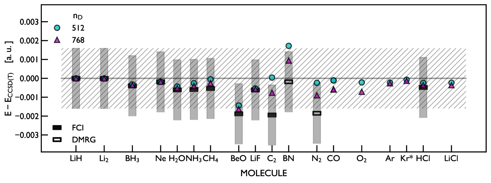
Figure 1: Energy differences with respect to CCSD(T) in the cc-pVDZ basis set. The shaded area indicates results within chemical accuracy (1 kcal/mol) from FCI/DMRG, and the hatched area from CCSD(T). Geometries and FCI reference energies (where available) are taken from Ref. [21], with the exception of the N₂ molecule at the distance of $2.118$ $a.u.$, where we compare to DMRG results from Ref. [22], and BN with our own calculation using the block2 code [23]. The molecules are ordered w.r.t increasing number of electrons, grouping those with equal numbers together. For those marked with ^* we employed a particle-hole transformation.

SDs also play a crucial role in many-body methods such as Quantum Monte Carlo. Compact SD expansions serve as efficient trial wavefunctions in Auxiliary-Field Quantum Monte Carlo (AFQMC) [24, 25, 26, 27] and Diffusion Monte Carlo (DMC) [28], and underpin variational ansätze like the Slater-Jastrow form [29] as well as recent variants augmented with neural networks [30, 31, 32, 33, 34, 35].

In this work, we show that a sum of fewer than a thousand non-orthogonal SDs is sufficient to accurately represent the all-electron ground-state wavefunction of small-size molecules, with energies that are competitive with state-of-the-art methods and with a favorable scaling as the fourth power of the basis set size. This result is obtained with a novel variational optimization technique we introduce here, based on an efficient analytical evaluation of the Hessian of the variational energy and the exact optimization of the energy as a function of one orbital for each determinant. We benchmark the accuracy for various molecules in the cc-pVDZ basis with full-CI data where available, and with DMRG and coupled-cluster with up to perturbative triple excitations otherwise. We find that our variational energies are consistently below coupled cluster, and within chemical accuracy of full-CI and DMRG.

Results

The Unconstrained Configuration Interaction (UCI) ansatz.

The wave function we consider consists of a sum of SDs with fixed number of spin-up and spin-down electrons

$$\ket{\bar{\Phi}}=\sum_{I=1}^{N_{D}}\ket*{\Phi^{(I\uparrow)}}\otimes\ket*{\Phi^{(I\downarrow)}},$$ (1)

where $N_{D}$ is the number of determinants, and

$$\ket*{\Phi^{(I,\sigma)}}=\prod_{i=1}^{n_{\sigma}}\Big{(}\sum_{\mu=1}^{m}\phi_{i,\mu}^{(I,\sigma)}\hat{c}^{\dagger}_{\mu,\sigma}\Big{)}\ket{{0}}$$ (2)

are non-orthogonal Slater determinants, with independent “MO orbitals” $\phi^{(I,\sigma)}_{i}\in\mathbb{C}^{m}$, where $n_{\sigma}$ is the number of electrons with spin $\sigma\in\{\uparrow,\downarrow\}$, $m$ is the number of basis orbitals and $\hat{c}_{\mu,\sigma}^{\dagger}$ is the creation operator of an electron in orbital $\mu$ with spin $\sigma$. We refer to this wavefunction as unconstrained configuration interaction (UCI) ansatz.

The SD optimization strategy we introduce in this work, as detailed in the Methods section, is based on two facts: (i) the average energy of the UCI wavefunction of Eq.˜1 is the ratio of two quadratic functions of $\phi^{(I,\sigma)}_{i}$, which implies that these parameters can be optimized exactly, and the procedure repeated; (ii) the needed effective Hamiltonian matrix can be computed with a total computational cost of $O(m^{4})$ with an efficient tensor-contraction strategy.

Benchmark for equilibrium geometries in the cc-pVDZ basis with CCSD(T), DMRG and FCI.

To validate the accuracy of the proposed method, we compare it against CCSD(T), and, where available, DMRG and FCI, for the all-electron ground-state energy of several molecules at equilibrium in the cc-pVDZ basis set. The electron number varies from $4$ (LiH) to $20$ (for LiCl), except for the Krypton atom with $36$ electrons in $27$ orbitals, where we perform a particle-hole transformation to reduce the effective number of interacting particles to $18$. As reported in Fig.˜1, our optimized energies from up to $768$ Slater determinants are well within chemical accuracy (1 kcal/mol) with respect to FCI, including those at the limit of what is still tractable by current distributed FCI codes [21]. Furthermore, our variational energies are consistently below the ones obtained with coupled cluster at CCSD(T) level, even if energy comparisons with a non-variational method could appear to not be completely fair to our method. This is significant because CCSD(T) has an asymptotic computational scaling of $O(m^{7})$, while our method scales like $O(m^{4})$. For all molecules we find the expected spin symmetry for the ground state, with a maximal spin contamination at 768 determinants of $\absolutevalue*{\expectationvalue*{\hat{S}^{2}}-S(S+1)}$ $\approx 2\cdot 10^{-2}$ for BN, and much less for the other molecules. We also note that $768$ determinants consistently improve the results of $512$ determinants, and that the optimization steps to achieve convergence are roughly independent of the number of determinants (see Supplementary Information, Appendix˜A).

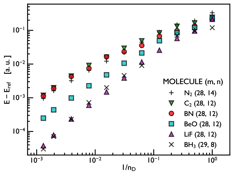
Figure 2: Scaling of the number of SDs with bond order. We consider here the four di-atomic molecules C₂, BN, BeO and LiF with an identical number of electrons and basis orbitals, and BH₃ and N₂ with similar numbers, all in the cc-pVDZ basis set. The molecules possess different bond orders, ranging from the single bond of LiF to the triple bond of N₂, explaining the different scaling of the error. Equilibrium geometries and FCI reference energies from Ref. [21], except for N₂ molecule at the distance of $2.118$ $a.u.$, where we compare to DMRG results from Ref. [22], and BN to our own DMRG calculation using the block2 code [23].

Scaling of the number of SDs with bond order.

In general, we expect the number of SDs needed to precisely model the ground state to increase with correlations, and, in particular, we expect a dependence on the number of valence electrons. To verify this picture in a controlled setting, we consider the three molecules LiF, BeO and N₂, which all have similar number of electrons, $12-14$, the same number of basis orbitals in the cc-pVDZ basis set, $28$, but different bond order. In Fig.˜2 we report the energy error w.r.t. FCI as a function of the number of SD ($1$ up to $768$), observing a smooth and consistent scaling. Moreover, the log-log plot graphically shows that the decay of the energy error is certainly not slower than a power-law of the inverse number of SDs. The slope of the decay clearly decreases with the bond order/number of valence electrons, meaning that for N₂ we need more than an order of magnitude more determinants to attain chemical accuracy than what is needed for LiF, with BeO lying in between. The single-bonded BH₃ shows a similar scaling as LiF, while it is interesting to remark that the curves for C₂ and BN nearly collapse on the one of the triple-bonded N₂.

Convergence to the large-basis-set limit.

In Fig.˜3 we consider the ground-state energy of the LiH molecule at equilibrium distance, for various basis sets of sizes ranging from $6$ to $146$ orbitals, the largest for which FCI energies are still available [21]. The approximate curve collapse for the energy error in a given basis set as a function of the ratio of the number of SDs and the basis set size $m$, shown in the inset of Fig.˜3, suggests that the number of determinants needed to get a fixed error in a given basis scales linearly with the basis set size. We conjecture that this might be due to the short-distance cusp conditions of the continuum-space wave function, which require having a UCI with an increasing number of determinants in the approach to the continuum limit. Nevertheless, as we show in the main plot of Fig.˜3, the absolute energy decreases with increasing basis set size for a fixed number of SD, as does the error with respect to the true ground-state energy in the infinite-basis-set limit.

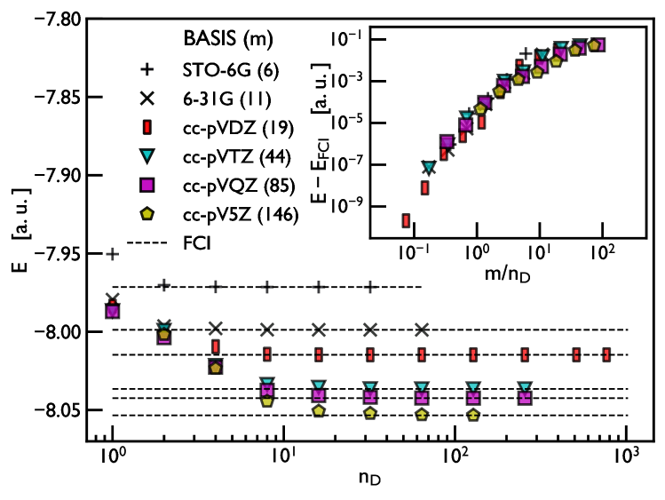
Figure 3: Convergence to the infinite-basis-set limit. We show the absolute energy convergence as a function of the number of SD and the basis-set size for LiH. In the inset, we show an approximate curve collapse of the absolute error with respect to FCI in a given basis as a function of the ratio between the size of the basis and the number of SD. We use equilibrium geometry and FCI reference energies from Ref. [21] (dashed lines).

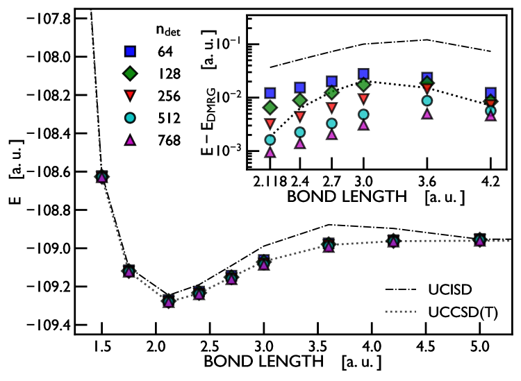
Figure 4: Dissociation curve of the N₂ molecule in the cc-pVDZ basis. In the inset we show the error compared to DMRG results from Ref. [22] for the equilibrium bond distance and larger, and we also compare with UCISD and UCCSD(T).

Capturing static correlations.

As a prototypical example of bond breaking we consider the Nitrogen molecule. As its bond is stretched, the wavefunction starts to have an inherent multireference character. Single reference methods such as CISD and CCSD(T) start to struggle, converging more slowly or not converging at all [22]. In Fig.˜4 we show the dissociation curve or the N₂ molecule in comparison with UCISD (which uses 30724 determinants), UCCSD(T) and DMRG. We outperform UCISD and UCCSD(T) already with a few hundred independent Slater determinants. As can be seen in the inset, close to equilibrium we obtain energies within chemical accuracy from DMRG, however not at large distances.

Triplet and singlet dioxygen states.

As an additional application, we discuss the low-energy states of molecular oxygen for different sectors of the $M$ and $S$ quantum numbers. While ${M=\expectationvalue*{\hat{S}_{z}}=\frac{1}{2}(n^{\uparrow}{-}n^{\downarrow})}$ is directly imposed in the wavefunction, for $S$ we instead add a $\lambda\,\hat{S}^{2}$ penalty term to the Hamiltonian, at no extra cost during the optimization. In Fig.˜5 we study the convergence of the O₂ to its triplet ground state, both in the $M=0$ and $M=1$ spin sectors. For the latter we need fewer determinants to accurately represent the eigenstate, due to the smaller size of the subspace it is defined in. Adding the $\lambda\,\hat{S}^{2}$ penalty term, with $\lambda=0.1$, we converge to the singlet state, which is known to be the first excited state of this molecule. In the inset, showing the total spin quantum number $S$, estimated from $\expectationvalue*{\hat{S}^{2}}=S(S+1)$, we show that we do not observe spin contamination, apart from the lowest number of determinants in the $M=0$ sector.

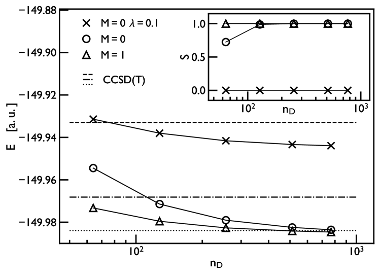
Figure 5: Triplet ground state and singlet first excited state of the O₂ molecule in the cc-pVDZ basis set. The singlet state is found by minimizing the energy of the Hamiltonian with an additive penalty term $\lambda\,\hat{S}^{2}$. The horizontal lines represent CCSD(T) energies for ${M=0}$ ${S=0}$ (dashed), ${M=0}$ ${S=1}$ (dash-dotted) and ${M=1}$ ${S=1}$(dotted). Equilibrium geometry taken from the supplementary material of Ref. [21].

Discussion

We have introduced a deterministic algorithm for the variational optimization of a sum of nonorthogonal SDs with favorable $\mathcal{O}(m^{4})$ scaling with the basis set size. Our results show that it is possible to achieve chemical accuracy with respect to full-CI and DMRG calculations in the correlation-consistent double-zeta basis with just a few hundred determinants, and to consistently obtain variational energies lower than coupled-cluster CCSD(T) methods. We have further demonstrated that the SD ansatz can be highly accurate for large basis-set sizes when compared to FCI for small molecules, and that we are able to accurately capture the strong correlations occurring at bond breaking of N₂. In addition, we have shown that only a relatively small number of SDs are needed to recover the expected symmetry-eigenstates of the O₂ molecule.

The computational bottleneck of our method is the memory needed to densely store the $\mathcal{H}$ and $\mathcal{S}$ matrices used to solve the generalized eigenvalue problem. However, as matrix-vector products with $\mathcal{H}$ and $\mathcal{S}$ can be computed efficiently, iterative solvers could be used instead. Alternatively, with a similar formalism, we could optimize a subset of all the determinants at each step, or optimize determinants that share some orbitals, which could also be useful to enforce symmetries and further decrease spin contamination. The efficiently contractable formulae Eqs.˜18 and 19 naturally admit tensor decompositions of the Hamiltonian [36, 37] with the potential to further reduce the computational scaling in $m$ for computing the $\mathcal{H}$ matrix. A more physical limitation of the method is size inconsistency at fixed number of determinants: in order to have the same accuracy on a system consisting of two non-interacting parts, the number of determinants should be higher than the number of determinants used in each subsystem, as we show in Appendix˜A. Another limitation is the inability of sums of Slater Determinants to represent the cusp of the wave function in the continuum limit. As discussed in the Results section, we conjecture that this is responsible for the linear increase of the number of determinants with the number of basis set orbitals, for fixed precision in a given basis set, even if the overall accuracy is increasing with larger basis set when compared to the infinite-basis-set limit. The wave-function cusp could be directly imposed by adding a Jastrow factor to the optimized Slater determinants, and further optimizing it with VMC.

A straightforward extension of this work is to evaluate the first excited states. As we have an analytical expression for wave-function overlaps, we can directly project out the UCI ground state (or any other subspace) from a UCI state, and variationally optimize the energy, which remains a quadratic function. It is also possible to extend the technique to time evolution, both in real and imaginary time. The approach is very similar to the one presented in this work, as the fidelity optimization is also a ratio of quadratic function in the orbitals. While we leave discussions of extrapolations to the infinite-determinant limit for future work, we note that we are able to compute the variance of the energy with the same computational cost as the energy, which could be used to obtain a better estimate of the ground state using the zero-variance principle.

We have introduced our approach as a standalone method. However, it could also be used in conjunction with other established methods. For example, it could provide a highly accurate multideterminant trial wavefunction for AFQMC and DMC calculations, requiring a much lower number of determinants and a higher fidelity compared to the CI wavefunctions typically used. The UCI Ansatz, trained with the analytical orbital optimization strategy of the present article, typically outperforms state-of-the-art second-quantized VMC approaches using artificial neural networks. Nevertheless, determinant-based variational Ansätze, augmented by neural networks, in first or second quantization, with pre-optimized determinant parts could be a promising approach for VMC.

Methods

Notation.

We use capital letters for many-body quantities: $\ket*{\bar{\Phi}}$, $\ket*{\Phi^{(I)}}$ denote $n$-electron wavefunctions, $N_{D}$ is the number of determinants, and $I,J,K,\dots\in\{1,\dots,N_{D}\}$ are determinant labels. For single electron quantities we use lowercase letters: $n$ is the number of electrons, $i,j,\dots\in\{1,\dots,n\}$ are electron labels, $m$ is the number of basis functions, and $\mu,\nu,\dots\in\{1,\dots,m\}$ bare basis orbitals labels. $\hat{c}^{\dagger}_{\mu}$ is the creation operator creating an electron in the $\mu$th basis state (assumed here, for simplicity, to be orthonormal for the usual anticommutation relations to hold).

We consider the UCI ansatz

$$\ket*{\bar{\Phi}}=\sum_{I=1}^{N_{D}}\ket*{\Phi^{(I)}}$$ (3)

given by a sum of non-orthogonal SDs $\ket*{\Phi^{(I)}}$. Each determinant $I$ is fully specified by its own set of “MO orbitals” $\{\phi^{(I)}_{1},\phi^{(I)}_{2},\dots,\phi^{(I)}_{n}\}$, given as a column vector of coefficients, i.e. $\phi^{(I)}_{i}\in\mathbb{C}^{m}$. With the operators for creating an electron in the $i$’th MO orbital of determinant $I$, given by $\hat{b}^{(I)\dagger}_{i}=\sum_{\mu}\phi_{i,\mu}^{(I)}\hat{c}^{\dagger}_{\mu}$ we can build each SD as

$$\ket*{\Phi^{(I)}} =\hat{b}^{(I)\dagger}_{1}\hat{b}^{(I)\dagger}_{2}\cdots\hat{b}^{(I)\dagger}_{n}\ket{{0}}$$ (4)

$$=\big{(}\sum_{\mu_{1}}\phi_{1,\mu_{1}}^{(I)}\hat{c}^{\dagger}_{\mu_{1}}\big{)}\big{(}\sum_{\mu_{2}}\phi_{2,\mu_{2}}^{(I)}\hat{c}^{\dagger}_{\mu_{2}}\big{)}\cdots\big{(}\sum_{\mu_{n}}\phi_{i_{n},\mu_{n}}^{(I)}\hat{c}^{\dagger}_{\mu_{n}}\big{)}\ket{{0}}$$

In this parametrization the determinant is multilinear in the MO orbital coefficient vectors $\phi^{(I)}_{i}$, and linear when viewed as a function of a single one of them. Without loss of generality, singling out the first orbital (it is just a matter of reordering the orbitals in every determinant, and absorbing the resulting sign into one of the coefficient vectors), we have that

$$\ket*{\Phi^{(I)}} =\hat{b}^{(I)\dagger}_{1}\ket*{\Phi^{(I)}_{\text{1+}}} =\sum_{\mu}\phi_{1,\mu}^{(I)}\hat{c}_{\mu}^{\dagger}\ket*{\Phi^{(I)}_{\text{1+}}}$$ (5)

where $\ket*{\Phi^{(I)}_{\text{1+}}}\coloneqq\hat{b}^{(I)\dagger}_{2}\cdots\hat{b}^{(I)\dagger}_{n}\ket*{{0}}$ is a “hole”-SD, i.e. the $I$^th SD with the first electron removed. We can write the full UCI wavefunction, in terms of the “hole”-SD’s as

$$\ket*{\bar{\Phi}}=\sum_{I}\sum_{\mu}\phi_{1,\mu}^{(I)}\hat{c}_{\mu}^{\dagger}\ket*{\Phi^{(I)}_{\text{1+}}}$$ (6)

Optimization algorithm.

Our first observation is that, when regarded as a function of a single orbital of each SD like this, the energy expectation value becomes a simple ratio of two quadratic forms

$$E=\frac{\matrixelement*{\bar{\Psi}}{\hat{H}}{\bar{\Psi}}}{\innerproduct*{\bar{\Psi}}{\bar{\Psi}}}=\frac{v^{\dagger}\mathcal{H}v}{v^{\dagger}\mathcal{S}v}$$ (7)

where $v\in\mathbb{C}^{(N_{D}\times m)}$,

$$v_{I\mu}=\phi^{(I)}_{1,\mu}$$ (8)

is the “vector” (with flattened index $I\mu$) containing the orbitals we factored out from each determinant and $\mathcal{H},\mathcal{S}\in\mathbb{C}^{(N_{D}\times m)\times(N_{D}\times m)}$ are the “effective matrices” for the Hamiltonian and the identity, given by

$$\mathcal{H}_{I\mu,J\nu}=\matrixelement*{\Phi^{(I)}_{\text{1+}}}{\hat{c}_{\mu}\hat{H}\hat{c}_{\nu}^{\dagger}}{\Phi^{(J)}_{\text{1+}}}$$ (9)

$$\mathcal{S}_{I\mu,J\nu}=\matrixelement*{\Phi^{(I)}_{\text{1+}}}{\hat{c}_{\mu}\hat{c}_{\nu}^{\dagger}}{\Phi^{(J)}_{\text{1+}}}.$$ (10)

The energy Eq.˜7 takes the form of a generalized Rayleigh quotient, and can be minimized exactly w.r.t. $v$ by solving the generalized eigenvalue problem (GEV)

$$\mathcal{H}v=\epsilon\,\mathcal{S}v$$ (11)

taking $\mathcal{O}({N_{D}}^{3}\,{m}^{3})$ operations. We remark that $S$ (and $\mathcal{H}$) are singular, with nullspace spanned by the ’MO orbitals’ of the hole-SD’s $\ket*{\Phi^{(I)}_{\text{1+}}}$. By projecting it out, the problem can be reduced from $N_{D}\times m$ to a smaller eigenvalue problem of size $N_{D}(m{-}n{+}1)$.

Our second observation is that the effective Hamiltonian matrices $\mathcal{H}$ and $\mathcal{S}$ can be calculated efficiently. By contracting the tensors in the corresponding equations in an efficient order, $\mathcal{H}$ can be calculated in a numerically-exact way at the same $\mathcal{O}({N_{D}^{2}\,m}^{4})$ asymptotic cost as the energy expectation value, and $\mathcal{S}$ at a cost of $\mathcal{O}({N_{D}^{2}\,m}^{2})$, as we elaborate on in the next paragraph.

The procedure described so far minimizes the energy with respect to a single “MO orbital” of each SD, and different orbitals can be optimized by permuting their order in each determinant. More generally, we can mix the MO orbitals of each determinant with a random unitary matrix $U^{(I)}\in U(n)$, where $U(n)$ is the unitary group, obtaining the transformed orbitals

$$\phi^{(I)}_{i}\longrightarrow\sum_{j}U_{i,j}^{(I)}\phi^{(I)}_{j},$$ (12)

and use it to construct an iterative method which eventually optimizes all orbitals, summarized in Algorithm˜1.

Algorithm 1 Sketch of the algorithm

Initialize Slater determinants

while not converged do

  Randomly rotate the orbitals $\phi^{(I)}\rightarrow U^{(I)}\phi^{(I)}$

  Build $\mathcal{H}$ and $\mathcal{S}$

  Solve the GEV $\mathcal{H}v=\epsilon\mathcal{S}v$

  Update $\phi_{1}^{(I)}$ in each SD $I$

end while

We discuss the generalization to spinful electrons for the wavefunction Eq.˜1 in Appendix˜B.

Efficient calculation of the effective matrices.

We briefly discuss how to compute the matrices $\mathcal{H}$ and $\mathcal{S}$ in an efficient and numerically stable way. Given two Slater determinants $\ket{\Phi},\ket{\Psi}$,

$$\innerproduct{\Phi}{\Psi}=\det[A]$$ (13)

where $A_{ij}=\phi_{i}^{\dagger}\psi_{j}=\sum_{\mu}\phi^{\star}_{i,\mu}\psi_{j,\nu}$ is the matrix of pairwise overlaps of the “MO orbitals”.

We consider a generic normal ordered $N$-body operator

$$\hat{W}=\sum_{\begin{subarray}{c}\xi_{1}\dots\xi_{N}\\ \zeta_{1}\zeta_{2}\dots\zeta_{N}\end{subarray}}w_{\xi_{1}\xi_{2}\dots i_{N}}^{\zeta_{1}\dots\zeta_{N}}{\hat{c}_{\zeta_{N}}^{\dagger}\dots c_{\zeta_{1}}^{\dagger}\hat{c}_{\xi_{1}}\dots\hat{c}_{\xi_{N}}}\\$$ (14)

and compute the matrix element value

$$\matrixelement{\Phi}{\hat{W}}{\Psi}=\sum_{\begin{subarray}{c}\xi_{1}\dots\xi_{N}\\ \zeta_{1}\dots\zeta_{N}\end{subarray}}w_{\xi_{1}\dots\xi_{N}}^{\zeta_{1}\dots\zeta_{N}}\,\rho_{\xi_{1}\dots\xi_{N}}^{\zeta_{1}\dots\zeta_{N}}$$ (15)

where

$$\rho_{\xi_{1}\dots\xi_{N}}^{\zeta_{1}\dots\zeta_{N}}=\matrixelement{\Phi}{\hat{c}_{\zeta_{N}}^{\dagger}\dots c_{\zeta_{1}}^{\dagger}\hat{c}_{\xi_{1}}\dots\hat{c}_{\xi_{N}}}{\Psi}$$ (16)

is the $N$-body reduced density matrix.

We start with the simplifying assumption that the overlap $\innerproduct{\Phi}{\Psi}$ is nonzero and write down the generalization to $N$-body of the well-known expression for 2-body operators [38, 39, 40, 41, 42, 43, 44] provided, e.g., in Eq. 30 of Ref. [42],

$$\rho_{\xi_{1}\dots\xi_{N}}^{\zeta_{1}\dots\zeta_{N}}=\det[A]\det{\begin{bmatrix}B^{\xi_{1}}_{\zeta_{1}}&\cdots&B^{\xi_{N}}_{\zeta_{1}}\\ \vdots&\ddots&\vdots\\ B^{\xi_{1}}_{\zeta_{N}}&\cdots&B^{\xi_{N}}_{\zeta_{N}}\end{bmatrix}}$$ (17)

where $B^{\xi}_{\zeta}=\sum_{i,j}\psi_{\xi,i}^{\star}\,(A^{-1})_{ij}\,\phi_{\zeta,j}$. See Appendix˜C for a derivation. Eq.˜17 has an overall computational cost of $\mathcal{O}(N^{3}\,m^{2N})$.

Efficiently-contractable formula.

In this work we consider $N\in\{0,1,2,3\}$, for which it is computationally feasible to expand the determinants of Eq.˜17 into its $N!$ terms, and directly contract them with $w$,

$$\frac{\matrixelement{\Phi}{\hat{W}}{\Psi}}{\innerproduct{\Phi}{\Psi}}=\sum_{\sigma\in S_{N}}\mathrm{sgn}(\sigma)\sum_{\begin{subarray}{c}\xi_{1}\dots\xi_{N}\\ \zeta_{1}\dots\zeta_{N}\end{subarray}}w_{\xi_{1}\dots\xi_{N}}^{\zeta_{1}\dots\zeta_{N}}\prod_{t=1}^{N}B^{\xi_{t}}_{\zeta_{\sigma[t]}},$$ (18)

where $\mathcal{S}_{N}$ is the symmetric group and $\sigma[t]$ is the $t$-th element of the permutation $\sigma$. Whenever $w_{\xi_{1}\dots\xi_{N}}^{\zeta_{1}\dots\zeta_{N}}$ admits a compact tensor decomposition, we can expect the application of Eq.˜18 to be advantageous. To give an example of this fact, we consider a factorizable 3-body operator given by $w_{\xi_{1}\xi_{2}\xi_{3}}^{\zeta_{1}\zeta_{2}\zeta_{3}}=w_{\xi_{1}\xi_{2}}^{\zeta_{1}\zeta_{2}}\,w_{\xi_{3}}^{\zeta_{3}}$ as we encounter in Eq.˜20. In this case, an application of the efficiently-contractable formula, Eq.˜18, requires only $\mathcal{O}(m^{4})$ operations, whereas using Eq.˜16 needs $\mathcal{O}(m^{6})$ operations.

For the zero-overlap case, $\innerproduct{\Phi}{\Psi}=\det[A]=0$, we decompose $A=U\Lambda V^{H}$ using the Singular Value Decomposition (SVD) and use the following equation (which we derive in Appendix˜D)

$$\matrixelement{\phi}{\hat{W}}{\Psi}=\det[U]\det[V^{H}]\sum_{\sigma\in S_{N}}\mathrm{sgn}(\sigma)$$ (19)

$$\quad\sum_{\begin{subarray}{c}\xi_{1}\dots\xi_{N}\\ \zeta_{1}\dots\zeta_{N}\end{subarray}}w_{\xi_{1}\dots\xi_{N}}^{\zeta_{1}\dots\zeta_{N}}\sum_{k_{1}\dots k_{N}}T_{k_{1}\dots k_{N}}\prod_{t=1}^{N}X_{\xi_{t},k_{t}}Y_{k_{t},\zeta_{\sigma[t]}},$$

where $X_{\xi,k}=\sum_{i}\psi_{i,\xi}^{\star}V_{i,k}$ and $Y_{k,\zeta}=\sum_{j}U^{\star}_{j,k}\phi_{j,\zeta}$. The tensor $T_{k_{1}\dots k_{N}}\in\mathbb{R}$ is the product of all singular values which are not indexed, defined as $T_{k_{1}\dots k_{N}}=\prod_{i\in\{1,\dots n\}\setminus\{k_{1},\dots,k_{N}\}}\Lambda_{i}$. This equation is correct regardless of the rank of $A$, and it is numerically stable whenever singular values are numerically close to zero. The contraction of Eq.˜19 has a computational cost larger by a factor of $\mathcal{O}(n)$ compared to Eq.˜18.

For the matrices $\mathcal{H}$ and $\mathcal{S}$, defined in Eq.˜9 and Eq.˜10, we need to calculate matrix elements of the form $\matrixelement*{\Phi}{\hat{c}_{\mu}\hat{W}\hat{c}_{\nu}^{\dagger}}{\Psi}$ for all $\mu,\nu\in\{1,\dots,m\}$ where $\hat{W}$ is a $N$-body operator (see Eq.˜14) and thus $\hat{c}_{\mu}\hat{W}\hat{c}_{\nu}^{\dagger}$ is a ${N{+}1}$-body operator. In the following we show that calculating $\matrixelement*{\Phi}{\hat{c}_{\mu}\hat{W}\hat{c}_{\nu}^{\dagger}}{\Psi}$ for all $\mu,\nu\in\{1,\dots,m\}$ has the same asymptotic cost in $m$ as $\matrixelement*{\Phi}{\hat{W}}{\Psi}$.

Using Wick’s theorem [45], or repeated application of the fermionic anticommutation relations, $\hat{c}_{\mu}\hat{W}\hat{c}_{\nu}^{\dagger}$ can be brought into normal order, resulting in a sum of ${N{+}1}$, $N$ and ${N{-}1}$-body operators.

For $N\geq 1$, in the nonzero-overlap case $\innerproduct{\phi}{\Psi}\neq 0$, so that we can use Eq.˜18, we have that

$$\frac{\matrixelement*{\Phi}{\hat{c}_{\mu}\hat{W}\hat{c}_{\nu}^{\dagger}}{\Psi}}{\innerproduct{\Phi}{\Psi}}=$$ (20)

$$-\sum_{\mathclap{\sigma\in S_{N+1}}}\mathrm{sgn}(\sigma)\,w_{\xi_{1}\dots\xi_{N}}^{\zeta_{1}\dots\zeta_{N}}\prod_{t=1}^{N+1}B^{\xi_{t}}_{\zeta_{\sigma[t]}}$$

$$+\delta_{\mu,\nu}\sum_{\mathclap{\sigma\in S_{N}}}\mathrm{sgn}(\sigma)\,w_{\xi_{1}\dots\xi_{N}}^{\zeta_{1}\dots\zeta_{N}}\prod_{t=1}^{N}B^{\xi_{t}}_{\zeta_{\sigma[t]}}$$

$$-\sum_{\mathclap{\begin{subarray}{c}\sigma\in S_{N-1}\\ u\in\{1,\dots,N\}\end{subarray}}}\mathrm{sgn}(\sigma)\,w_{\xi_{1}\dots\xi_{N}}^{\zeta_{1}\dots\zeta_{u-1}\,\mu\,\zeta_{u+1}\dots\zeta_{N}}\prod_{t=1}^{N}B^{\xi_{t}}_{\zeta_{\sigma[t]}}$$

$$-\sum_{\mathclap{\begin{subarray}{c}\sigma\in S_{N-1}\\ v\in\{1,\dots,N\}\end{subarray}}}\mathrm{sgn}(\sigma)\,w_{\xi_{1}\dots\xi_{v-1}\,\nu\,\xi_{v+1}\dots\xi_{N}}^{\zeta_{1}\dots\zeta_{N}}\prod_{t=1}^{N}B^{\xi_{t}}_{\zeta_{\sigma[t]}}$$

$$+\sum_{\mathclap{\begin{subarray}{c}\sigma\in S_{N-1}\\ u,v\in\{1,\dots,N\}\end{subarray}}}\mathrm{sgn}(\sigma)\,(-1)^{u+v}\,w_{\xi_{1}\dots\xi_{v\text{-}1}\,\nu\,\xi_{v}\dots\xi_{N\text{-}1}}^{\zeta_{1}\dots\zeta_{u\text{-}1}\,\mu\,\zeta_{u}\dots\zeta_{N\text{-}1}}\prod_{t=1}^{N\text{-}1}B^{\xi_{t}}_{\zeta_{\sigma[t]}}$$

where we take $\xi_{N+1}\equiv\mu$ and $\zeta_{N+1}\equiv\nu$ for the first term, $\zeta_{u}\equiv\nu$ for the third and $\xi_{v}\equiv\mu$ in the fourth, and use Einstein summation for the remaining $\xi$ and $\zeta$ indices. The tensors in the equation can be contracted in such a way that the cost is $\mathcal{O}((N+1)!\,m^{2N})$.

It can be shown that also in the zero-overlap case, using Eq.˜19, the tensors can be contracted in ${\mathcal{O}((N+1)!\,m^{2N}\,n)}$. We provide the full equation in Appendix˜E.

For the special case $N=0$, for $\mathcal{S}$, we get

$$\frac{\matrixelement*{\Phi}{\hat{c}_{\mu}\hat{c}_{\nu}^{\dagger}}{\Psi}}{\innerproduct*{\Phi}{\Psi}}=-B^{\mu}{\nu}+\delta_{\mu,\nu},$$ (21)

where both terms can be computed in $\mathcal{O}(m^{2})$.

We use Eq.˜20 and Eq.˜21 to compute the matrices Eq.˜9 and Eq.˜10. Given a generic 2-body Hamiltonian $\hat{H}$, this results in a computational cost of $\mathcal{O}(N_{D}^{2}m^{4})$.

Acknowledgements

We thank F. Vicentini and L. Viteritti for discussions. This work was supported by the Swiss National Science Foundation under Grant No. 200021_200336. This research was also supported by SEFRI through Grant No. MB22.00051 (NEQS - Neural Quantum Simulation)

Supplementary Material

Implementation details

We work with the second quantized formulation of the electronic/molecular Hamiltonian in a finite basis set of size $m$, given by

$$\hat{H}=\sum_{\begin{subarray}{c}ij\\ \sigma\end{subarray}}h_{ij}\,\hat{c}_{i\sigma}^{\dagger}\hat{c}_{j\sigma}+\frac{1}{2}\sum_{\begin{subarray}{c}ijk\ell\\ \sigma\sigma^{\prime}\end{subarray}}h_{ijk\ell}\,\hat{c}_{i\sigma}^{\dagger}\hat{c}_{k\sigma^{\prime}}^{\dagger}\hat{c}_{l\sigma^{\prime}}\hat{c}_{j\sigma}+E_{\textrm{nuc}}$$ (22)

where $i,j,k,\ell\in\{1,\dots,m\}$ and $\sigma,\sigma^{\prime}\in\{\uparrow,\downarrow\}$.

We get the values for the one-and two electron integrals ($h_{ijk\ell},h_{ij},E_{nuc}$) of the Hamiltonian Eq.˜22 from PySCF [46, 47, 48], work in the molecular orbital basis and use complex-valued Slater determinants in double precision unless otherwise specified. We remark that the $\mathcal{O}(m^{5})$ scaling of transforming the two-electron integral explictly into an orthogonal basis can be straightforwardly reduced to $\mathcal{O}(m^{4})$, by including it in Eq.˜18/(19) and contracting the tensors in an efficient order.

To improve the overall numerical stability we work with normalized determinants $\frac{\ket*{\Psi^{(I)}}}{\norm{\ket*{\Psi^{(I)}}}}$ internally. We remark that the linear variational problem $\ket{\bar{\Psi}}=\sum_{I}c_{I}\frac{\ket*{\Psi^{(I)}}}{\norm{\ket*{\Psi^{(I)}}}}$ is automatically taken care of when we solve the eigenvalue problem Eq.˜11, with the coefficients $c_{I}$ being contained in $v$. Furthermore, we orthogonalize the orbitals of every determinant $\ket*{\Psi^{(I)}}$ separately using a QR decomposition of the non-square matrices ${\begin{bmatrix}\phi^{(I)}_{1}&\phi^{(I)}_{2}&\dots&\phi^{(I)}_{n}\end{bmatrix}}\in\mathbb{C}^{m\times n}$.

Appendix A Additional Results

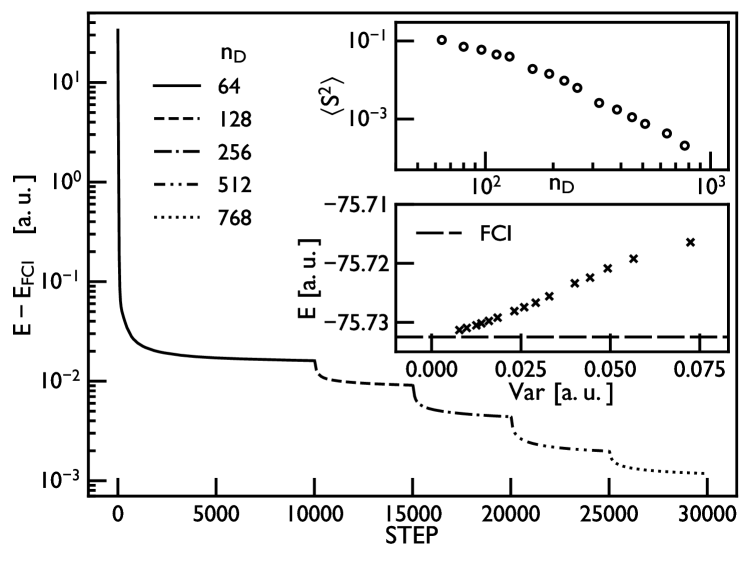
Figure 6: Convergence of the method as a function of the number of iteration steps for the C₂ molecule at equilibrium in the cc-pVDZ basis set. We compare to the exact FCI energy at the geometry provided in the supplermentary material of Ref. [21]. We optimized the first 64 determinants from scratch, and subsequently pre-initialized a part of the determinants using the ones from the previous run upon increasing the number of determinants. One step comprises the optimization of a single orbital of each of the $N_{D}$ determinants.

Convergence

In Fig.˜6 we show the convergence to the ground state of the C₂ molecule as a function of the iteration steps, where one step comprises the optimization of one orbtial of each determinant. While in principle we could optimize all Slater determinants from scratch, to reduce the computational cost, we re-use the already optimized Slater Determinants from the previous simulation, adding additional randomly initialized determinants. We observe a very smooth convergence, with energies which are strictly decreasing at every step. This is expected, as, by definition the energy cannot decrease in our method (unless caused by numerical instabilities). We further remark that, when using complex-valued determinants we do not observe any orthogonal determinants during the energy optimization, meaning that we can use Eq.˜18 and do not have to resort to Eq.˜19. However, during testing with real-valued determinants we did observe numerical instabilities requiring the use of the stable svd formula Eq.˜19. In the first inset of Fig.˜6 we plot the expectation value of the total spin squared operator, defined as (see e.g [49, Chapter 2])

$$\hat{S}^{2}=\frac{1}{2}(n^{\downarrow}+n^{\uparrow})+\frac{1}{4}(n^{\downarrow}-n^{\uparrow})^{2}-\sum_{t,u=1}^{m}\hat{c}^{\dagger}_{i\uparrow}\hat{c}_{j\uparrow}\hat{c}^{\dagger}_{j\downarrow}\hat{c}_{i\downarrow}$$ (23)

where $\expectationvalue*{\hat{S}_{z}}=\frac{1}{2}(n^{\uparrow}-n^{\downarrow})$ is fixed in the wavefunction, and $\expectationvalue*{\hat{S}^{2}}=S(S+1)$ for an Eigenstate of the Hamiltonian. Using the formulation from Eq.˜23 we can estimate $\expectationvalue*{\hat{S}^{2}}$ using a number of operations which scales as $\mathcal{O}({m}^{2})$ in $m$, the same cost as a generic 1-body operator. While for the smaller sizes we observe a small amount of spin contamination for this molecule, the expected value of $S$ goes to 0 using a power-law like behavior as the number of determinants is increased. Alternatively we could add a penalty term as described in the main text in the context of excited states. We further compute the energy variance, given by

$$\textrm{Var}=\expectationvalue*{\hat{H}^{2}}-\expectationvalue*{\hat{H}}^{2}.$$ (24)

Using the efficiently contractable formulae Eqs.˜18 and 19 (requiring $K=4$) we can compute the expectation value of $\hat{H}^{2}$ at the same asymptotic $\mathcal{O}({m}^{4})$ cost with the number of basis functions, as the expectation value of the energy itself. In the second inset of Fig.˜6 we provide an energy/variance plot, of the converged energies from $64$ to $768$ determinants, where we are in the approximately linear regime, suggesting that our states are close to the ground state.

Size Consistency

We plot in Fig.˜7 the difference in energy of the ground state of a molecule composed of two N atoms put at very large distance and the sum of the ground state energies of the single atoms, at fixed number of determinants. The fact that the difference is non zero is a proof of the non-size consistency of the ansatz at fixed number of determinants.

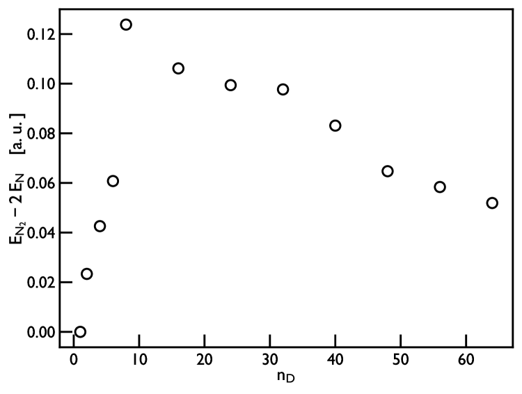
Figure 7: Size consistency. We plot the energy difference between the ground state of the N₂ molecule at an approximately infinite bond length compared to twice the energy of a single atom of Nitrogen, using an equal number of determinants.

Appendix B Generalization to spinful electrons

Algorithm˜1 can be generalized to optimize the wavefunction defined in Eqs.˜1 and 2 by modifying it as follows: At every step we choose to either optimize either the $(I,\uparrow)$ or the $(I,\downarrow)$ part, by sampling $\sigma_{I}\sim\mathrm{Unif}(\uparrow,\downarrow)$ iid. Then the vector $v_{I\mu}=\phi^{(I,\sigma_{I})}_{1,\mu}$ contains the $\uparrow/\downarrow$ orbitals as chosen, $\mathcal{H}$ can be computed as

$$\mathcal{H}_{I\mu,J\nu}=\sum_{\mu^{\prime}\nu^{\prime}}\phi^{(I,\bar{\sigma}_{I})\star}_{1,\mu^{\prime}}\phi^{(J,\bar{\sigma}_{J})}_{1,\nu^{\prime}}$$ (25)

$$\bra*{\Phi^{(I,\uparrow)}_{\text{1+}}}\otimes\bra*{\Phi^{(I,\downarrow)}_{\text{1+}}}{\hat{c}_{\mu^{\prime},\bar{\sigma}_{I}}\hat{c}_{\mu,\sigma_{I}}\hat{H}\hat{c}_{\nu,\sigma_{J}}^{\dagger}\hat{c}_{\nu^{\prime},\bar{\sigma}_{J}}^{\dagger}}\ket*{\Phi^{(J)}_{\text{1+}}}\otimes\ket*{\Phi^{(J)}_{\text{1+}}}$$

where we use the notation $\bar{\uparrow}=\downarrow$ and $\bar{\downarrow}=\uparrow$ for flipping the spin variables. $\mathcal{S}$ can be calculated analogously, replacing $\hat{H}$ with the identity. For the terms in the Hamiltonian which act only on the spin-up or spin-down electrons this factorizes, and we can apply Eqs.˜20 and 21 separately to the spin-up and spin-down terms. This is the case for all the terms in the Hamiltonian Eq.˜22, with the exception of the 2-body interaction term for $\sigma\neq\sigma^{\prime}$. For the latter the fermionic operators can be reordered as aproduct of two hopping terms for spin-up and spin-down, allowing the application of two instances of Eq.˜18/(19) with $N=1$. They can be contracted concurrently, resulting in an overall scaling in $m$ of $\mathcal{O}({m}^{4})$.

Appendix C Proof of the N-body normal order matrix element value formula

We recall the well-known Schur Complement formula for the determinant of a block matrix, given by

$$\det{\begin{bmatrix}A&B\\ C&D\end{bmatrix}}=\lim_{\varepsilon\to 0}\det[A+\varepsilon I]\det[D-C(A+\varepsilon I)^{-1}B]$$ (26)

where we added a infinitesimal diagonal shift $\varepsilon$ so that it can be applied when $A$ is singular.

In the following we prove

$$\matrixelement{\Phi}{\hat{c}_{\nu_{N}}^{\dagger}\dots c_{\nu_{1}}^{\dagger}\hat{c}_{\mu_{1}}\dots\hat{c}_{\mu_{N}}}{\Psi}=(-1)^{N}\det{\begin{bmatrix}A&\phi_{\nu_{1}}^{T}&\dots&\phi_{\nu_{N}}^{T}\\ \psi_{\mu_{1}}^{\star}&0&\dots&0\\ \vdots&\vdots&\ddots&\vdots\\ \psi_{\mu_{N}}^{\star}&0&\dots&0\\ \end{bmatrix}}$$ (27)

using

$$\matrixelement{\Phi}{\hat{c}_{\mu_{1}}\dots\hat{c}_{\mu_{N}}\hat{c}_{\nu_{N}}^{\dagger}\dots c_{\nu_{1}}^{\dagger}}{\Psi}=\det{\begin{bmatrix}A&\phi_{\nu_{1}}^{T}&\dots&\phi_{\nu_{N}}^{T}\\ \psi_{\mu_{1}}^{\star}&\delta_{\mu_{1}\nu_{1}}&\dots&\delta_{\mu_{1}\nu_{N}}\\ \vdots&\vdots&\ddots&\vdots\\ \psi_{\mu_{N}}^{\star}&\delta_{\mu_{N}\nu_{1}}&\dots&\delta_{\mu_{N}\nu_{N}}\\ \end{bmatrix}}$$ (28)

where $\mu_{u},\nu_{u}\in\{1\dots m\}$.

Proof By induction.

For the trivial $N=0$ case we have that $\innerproduct{\Phi}{\Psi}=\det[A]$. Alternatively, for $N=1$ we have that

$$\matrixelement{\Phi}{\hat{c}_{\nu_{1}}^{\dagger}\hat{c}_{\mu_{1}}}{\Psi} =\delta_{\mu_{1}\nu_{1}}\innerproduct{\Phi}{\Psi}-\matrixelement{\Phi}{\hat{c}_{\mu_{1}}\hat{c}_{\nu_{1}}^{\dagger}}{\Psi}$$ (29)

$$=\delta_{\mu_{1}\nu_{1}}\det[A]-\det{\begin{bmatrix}A&\phi_{\nu_{1}}^{T}\\ \psi_{\mu_{1}}^{\star}&\delta_{\mu_{1}\nu_{1}}\end{bmatrix}}$$

$$\overset{(\ref{eq:schur_block_det})}{=}\delta_{\mu_{1}\nu_{1}}\det[A]-\lim_{\varepsilon\to 0}\det[A+\varepsilon I]\big{(}\delta_{\mu_{1}\nu_{1}}-\psi_{\mu_{1}}^{\star}(A+\varepsilon I)^{-1}\phi_{\nu_{1}}^{T}\big{)}$$

$$\overset{(\ref{eq:schur_block_det})}{=}-\det{\begin{bmatrix}A&\phi_{\nu_{1}}^{T}\\ \psi_{\mu_{1}}^{\star}&0\end{bmatrix}}$$

The induction assumption is given by :

$$\matrixelement{\Phi}{\hat{c}_{\nu_{N}}^{\dagger}\dots c_{\nu_{1}}^{\dagger}\hat{c}_{\mu_{1}}\dots\hat{c}_{\mu_{N}}}{\Psi} \overset{(\ref{eq:interaction_generic_normal})}{=}(-1)^{N}\det{\begin{bmatrix}A&\phi_{\nu_{1}}^{T}&\dots&\phi_{\nu_{N}}^{T}\\ \psi_{\mu_{1}}^{\star}&0&\dots&0\\ \vdots&\vdots&\ddots&\vdots\\ \psi_{\mu_{N}}^{\star}&0&\dots&0\\ \end{bmatrix}}$$ (30)

$$\overset{(\ref{eq:schur_block_det})}{=}\lim_{\varepsilon\to 0}\det[A+\varepsilon I]\det[{\begin{bmatrix}\psi_{\mu_{t}}^{\star}&\dots&\psi_{\mu_{n}}^{\star}\end{bmatrix}}^{T}(A+\varepsilon I)^{-1}{\begin{bmatrix}\phi_{\nu_{1}}^{T}&\dots&\phi_{\nu_{N}}^{T}\end{bmatrix}}]$$

$$=\lim_{\varepsilon\to 0}\det[A+\varepsilon I]\sum_{\sigma\in S_{N}}\mathrm{sgn}(\sigma)\prod_{t=1}^{N}(\psi_{\mu_{t}}^{\star}(A+\varepsilon I)^{-1}\phi_{\nu_{\sigma[t]}}^{T})$$

Next we show the induction step, proving Eq.˜27 for $N>1$, assuming we have already shown it to up to $N-1$. We use the wick theorem [45] to express the antinormal string in normal order

$$\matrixelement{\Phi}{\hat{c}_{\mu_{1}}\dots\hat{c}_{\mu_{N}}\hat{c}_{\nu_{N}}^{\dagger}\dots c_{\nu_{1}}^{\dagger}}{\Psi}$$ (31)

$$\quad=\sum_{P=0}^{N}\sum_{(k_{1},l_{1})\neq\dots\neq(k_{P}l_{P})}\matrixelement{\Phi}{{\{}\wick{\hat{c}_{\mu_{1}}\c{2}\dots\c{1}{\hat{c}_{\mu_{k_{i}}}}\c{3}\dots c_{\mu_{N}}\hat{c}_{\nu_{N}}^{\dagger}\c{2}\dots\c{1}{\hat{c}_{\nu_{l_{i}}}^{\dagger}}\c{3}\dots\hat{c}_{\nu_{1}}^{\dagger}}{\}}}{\Psi}$$

$$\quad=\sum_{P=0}^{N}(-1)^{N-P}\sum_{\begin{subarray}{c}|\Omega|=P\\ \Omega\subset\{1,\dots,N\}\end{subarray}}\sum_{\begin{subarray}{c}|\Theta|=P\\ \Theta\subset\{1,\dots,N\}\end{subarray}}\sum_{\sigma\in S_{P}}\mathrm{sgn}(\sigma)\big{(}\prod_{t=1}^{P}\delta_{\mu_{\Omega_{t}}\nu_{\Theta_{\sigma[t]}}}(-1)^{\Omega_{t}+\Theta_{\sigma[t]}}\big{)}\matrixelement{\Phi}{\hat{c}_{\nu_{\bar{\Theta}_{N-P}}}^{\dagger}\dots\hat{c}_{\nu_{\bar{\Theta}_{1}}}^{\dagger}\hat{c}_{\mu_{\bar{\Omega}_{1}}}\dots c_{\mu_{\bar{\Omega}_{N-P}}}}{\Psi}$$

$$\quad=(-1)^{N}\matrixelement{\Phi}{\hat{c}_{\nu_{N}}^{\dagger}\dots\hat{c}_{\nu_{1}}^{\dagger}\hat{c}_{\mu_{1}}\dots c_{\mu_{N}}}{\Psi}$$

$$\quad\quad+\sum_{P=1}^{N}(-1)^{N-P}\sum_{\begin{subarray}{c}|\Omega|=P\\ \Omega\subset\{1,\dots,N\}\end{subarray}}\sum_{\begin{subarray}{c}|\Theta|=P\\ \Theta\subset\{1,\dots,N\}\end{subarray}}\sum_{\sigma\in S_{P}}\mathrm{sgn}(\sigma)\big{(}\prod_{t=1}^{P}\delta_{\mu_{\Omega_{t}}\nu_{\Theta_{\sigma[t]}}}(-1)^{\Omega_{t}+\Theta_{\sigma[t]}}\big{)}\matrixelement{\Phi}{\hat{c}_{\nu_{\bar{\Theta}_{N-P}}}^{\dagger}\dots\hat{c}_{\nu_{\bar{\Theta}_{1}}}^{\dagger}\hat{c}_{\mu_{\bar{\Omega}_{1}}}\dots c_{\mu_{\bar{\Omega}_{N-P}}}}{\Psi}$$

where $\wick{\c{1}\cdot\quad\c{1}\cdot}$ denotes the contraction, ${\{}\dots\}$ is the notation for normal ordering and $\bar{\Theta},\bar{\Omega}$ are the complements of the sets $\Theta$ and $\Omega$. Here we used that the only nonzero terms are those contracting $\hat{c}$ with $\hat{c}^{\dagger}$, thus it is sufficient that we consider all the possible combinations of their subsets of size $N$. The additional sign factor $(-1)^{\Omega_{t}+\Theta_{\sigma[t]}}$, comes from swapping the contracted operators to the center so that they are adjacent (after undoing the permutation $\sigma$ which results in the sign $\mathrm{sgn}(\sigma)$).
Solving for the normal ordered term $\matrixelement{\Phi}{\hat{c}_{\nu_{N}}^{\dagger}\dots\hat{c}_{\nu_{1}}^{\dagger}\hat{c}_{\mu_{1}}\dots c_{\mu_{N}}}{\Psi}$ it follows that

$$\matrixelement{\Phi}{\hat{c}_{\nu_{N}}^{\dagger}\dots\hat{c}_{\nu_{1}}^{\dagger}\hat{c}_{\mu_{1}}\dots c_{\mu_{N}}}{\Psi}$$ (32)

$$\quad=(-1)^{N}\matrixelement{\Phi}{\hat{c}_{\mu_{1}}\dots\hat{c}_{\mu_{N}}\hat{c}_{\nu_{N}}^{\dagger}\dots c_{\nu_{1}}^{\dagger}}{\Psi}$$

$$\quad\quad-\sum_{P=1}^{N}(-1)^{P}\sum_{\begin{subarray}{c}|\Omega|=P\\ \Omega\subset\{1,\dots,N\}\end{subarray}}\sum_{\begin{subarray}{c}|\Theta|=P\\ \Theta\subset\{1,\dots,P\}\end{subarray}}\sum_{\sigma\in S_{P}}\mathrm{sgn}(\sigma)\big{(}\prod_{i=1}^{P}\delta_{\mu_{\Omega_{t}}\nu_{\Theta_{\sigma[t]}}}(-1)^{\Omega_{t}+\Theta_{\sigma[t]}}\big{)}\matrixelement{\Phi}{\hat{c}_{\nu_{\bar{\Theta}_{P-N}}}^{\dagger}\dots\hat{c}_{\nu_{\bar{\Theta}_{1}}}^{\dagger}\hat{c}_{\mu_{\bar{\Omega}_{1}}}\dots c_{\mu_{\bar{\Omega}_{P-N}}}}{\Psi}$$

Using $\prod_{t=1}^{P}(-1)^{\Omega_{t}+\Theta_{\sigma[t]}}=(-1)^{\sum_{t=1}^{P}\Omega_{t}+\sum_{t=1}^{P}\Theta_{t}}$ to simplify Eq.˜32 we have that

$$\matrixelement{\Phi}{\hat{c}_{\nu_{P}}^{\dagger}\dots\hat{c}_{\nu_{1}}^{\dagger}\hat{c}_{\mu_{1}}\dots c_{\mu_{P}}}{\Psi}$$ (33)

$$\quad=(-1)^{P}\matrixelement{\Phi}{\hat{c}_{\mu_{1}}\dots\hat{c}_{\mu_{P}}\hat{c}_{\nu_{P}}^{\dagger}\dots c_{\nu_{1}}^{\dagger}}{\Psi}$$

$$\quad\quad-\sum_{P=1}^{N}\sum_{\begin{subarray}{c}|\Omega|=P\\ \Omega\subset\{1,\dots,P\}\end{subarray}}\sum_{\begin{subarray}{c}|\Theta|=P\\ \Theta\subset\{1,\dots,P\}\end{subarray}}(-1)^{\sum_{t=1}^{P}\Omega_{t}+\sum_{t=1}^{P}\Theta_{t}}\underbrace{(-1)^{P}\sum_{\sigma\in S_{P}}\mathrm{sgn}(\sigma)\big{(}\prod_{t=1}^{P}\delta_{\mu_{\Omega_{t}}\nu_{\Theta_{\sigma[t]}}}\big{)}}_{=\det{\begin{bmatrix}{-}\delta_{\mu_{\Omega_{t}}\nu_{\Theta_{u}}}\end{bmatrix}}_{t,u=1}^{P}}\underbrace{\matrixelement{\Phi}{\hat{c}_{\nu_{\bar{\Theta}_{P-N}}}^{\dagger}\dots\hat{c}_{\nu_{\bar{\Theta}_{1}}}^{\dagger}\hat{c}_{\mu_{\bar{\Omega}_{1}}}\dots c_{\mu_{\bar{\Omega}_{N-P}}}}{\Psi}}_{\overset{(\ref{eq:induction_assumption})}{=}\begin{subarray}{c}\lim_{\varepsilon\to 0}\det[A+\varepsilon I]\hfill\\ \cdot\det{\begin{bmatrix}\psi_{\mu_{\bar{\Omega}_{t}}}^{\star}(A+\varepsilon I)^{-1}\phi_{\nu_{\bar{\Theta}_{u}}}^{T}\end{bmatrix}}_{t,u=1}^{P-N}\end{subarray}}$$

Here we used the induction assumption Eq.˜30 for up to $N-P\leq N-1$. Next we add and subtract the $P=0$ term of the sum and simplify:

$$\matrixelement{\Phi}{\hat{c}_{\nu_{P}}^{\dagger}\dots\hat{c}_{\nu_{1}}^{\dagger}\hat{c}_{\mu_{1}}\dots c_{\mu_{P}}}{\Psi}$$ (34)

$$\quad=(-1)^{P}\matrixelement{\Phi}{\hat{c}_{\mu_{1}}\dots\hat{c}_{\mu_{P}}\hat{c}_{\nu_{P}}^{\dagger}\dots c_{\nu_{1}}^{\dagger}}{\Psi}$$

$$\quad\quad-\underbrace{\lim_{\varepsilon\to 0}\det[A+\varepsilon I]\underbrace{\sum_{P=0}^{N}\sum_{\begin{subarray}{c}|\Omega|=P\\ \Omega\subset\{1,\dots,P\}\end{subarray}}\sum_{\begin{subarray}{c}|\Theta|=P\\ \Theta\subset\{1,\dots,P\}\end{subarray}}(-1)^{\sum_{t=1}^{P}\Omega_{t}+\sum_{t=1}^{P}\Theta_{t}}\det{\begin{bmatrix}{-}\delta_{\mu_{\Omega_{t}}\nu_{\Theta_{j}}}\end{bmatrix}}_{t,u=1}^{P}\det{\begin{bmatrix}\psi_{\mu_{\bar{\Omega}_{t}}}^{\star}(A+\varepsilon I)^{-1}\phi_{\nu_{\bar{\Theta}_{j}}}^{T}\end{bmatrix}}_{t,u=1}^{P}}_{=\det{\begin{bmatrix}\psi_{\mu_{\bar{\Omega}_{t}}}^{\star}(A+\varepsilon I)^{-1}\phi_{\nu_{\bar{\Theta}_{j}}}^{T}-\delta_{\mu_{i}\nu_{j}}\end{bmatrix}}_{t,u=1}^{P}}}_{\overset{(\ref{eq:interaction_generic_antinormal})\&(\ref{eq:schur_block_det})}{=}(-1)^{P}\matrixelement{\Phi}{\hat{c}_{\mu_{1}}\dots c_{\mu_{P}}\hat{c}_{\nu_{P}}^{\dagger}\dots\hat{c}_{\nu_{1}}^{\dagger}}{\Psi}}$$

$$\quad\quad+\lim_{\varepsilon\to 0}\det[A+\varepsilon I]\det{\begin{bmatrix}-\psi_{\mu_{t}}^{\star}(A+\varepsilon I)^{-1}\phi_{\nu_{u}}^{T}\end{bmatrix}}_{t,u=1}^{P}$$

$$=\lim_{\varepsilon\to 0}\det[A+\varepsilon I]\det{\begin{bmatrix}-\psi_{\mu_{t}}^{\star}(A+\varepsilon I)^{-1}\phi_{\nu_{u}}^{T}\end{bmatrix}}_{t,u=1}^{P}\overset{(\ref{eq:schur_block_det})}{=}(-1)^{P}\det{\begin{bmatrix}A&\psi_{\nu_{1}}^{T}&\dots&\psi_{\nu_{P}}^{T}\\ \phi_{\mu_{1}}^{\star}&0&\dots&0\\ \vdots&\vdots&\ddots&\vdots\\ \phi_{\mu_{n}}^{\star}&0&\dots&0\end{bmatrix}}$$

where in the second step we used Eq.1 from Ref. [50] for the determinant of a sum two of matrices.

Appendix D Zero-overlap Formula

Starting from Eq.˜27 we apply Eq.˜26 and singular-value decompose $A=U\mathrm{S}V^{H}$ where $S$ is diagonal. Inserting the SVD for both $A$ and $A^{{-}1}$ we have that

$$\matrixelement{\Phi}{\hat{W}}{\Psi}=\lim_{\varepsilon\to 0}\det[U]\det[S+\varepsilon I]\det[V^{H}]\sum_{\begin{subarray}{c}\mu_{1}\dots\mu_{N}\\ \nu_{1}\dots b_{N}\end{subarray}}^{{n_{o}}}w_{\mu_{1}\dots\mu_{N}}^{\nu_{1}\dots\nu_{N}}\sum_{\begin{subarray}{c}i_{1}\dots i_{N}\\ j_{1}\dots j_{N}\\ k_{1}\dots k_{N}\end{subarray}}^{n_{e}}\sum_{\sigma\in S_{N}}\mathrm{sgn}(\sigma)\prod_{t=1}^{N}\psi_{\mu_{t},i_{t}}^{\star}V_{i_{t}k_{t}}(S_{k_{t}}+\varepsilon)^{-1}U^{\star}_{j_{t}k_{t}}\phi_{\nu_{\sigma[t]}j_{t}}$$ (35)

Here $(S+\varepsilon I)^{-1}$ is applied to an antisymmetric tensor, which is zero if the $\gamma_{i}$ are not distinct. This can be shown using the definition in terms of permutations of the generalized Kronecker delta,

$$\delta_{\nu_{1}\dots i_{N}}^{\nu_{1}\dots\nu_{N}}=\sum_{\sigma\in S_{N}}\mathrm{sgn}(\sigma)\delta_{\nu_{1}}^{\nu_{\sigma[1]}}\dots\delta_{\nu_{N}}^{\nu_{\sigma[N]}}$$ (36)

where $S_{N}$ is the symmetric group, as well as the following identity for moving the antisymmetrization

$$\sum_{x_{1}\dots x_{N}}\delta_{y_{1}\dots y_{N}}^{x_{1}\dots x_{N}}A_{x_{1}}^{z_{1}}A_{x_{2}}^{z_{2}}\dots A_{x_{N}}^{z_{N}}=\sum_{x^{\prime}_{1}\dots x^{\prime}_{N}}\delta_{x^{\prime}_{1}\dots x^{\prime}_{N}}^{z_{1}\dots z_{N}}A_{y_{1}}^{x^{\prime}_{1}}A_{y_{2}}^{x^{\prime}_{2}}\dots A_{z_{N}}^{x^{\prime}_{N}}$$ (37)

where $x_{u},y_{u}\in\{1,2,\dots,Q\}$ and $z_{u},x_{u}^{\prime}\in\{1,2,\dots,Q^{\prime}\}$ for all $x\in\{1,\dots,Q\}$ and arbitrary $Q,Q^{\prime}$. Then we can apply the following identity, which allows us to remove the singularity when one of the singular values is zero, taking the limit $\varepsilon\to 0$:

$$\lim_{\epsilon\to 0}\Big{(}\prod_{k=1}^{n}(\Lambda_{k}+\epsilon)\Big{)}\,\delta_{i_{1}\dots i_{N}}^{j_{1}\dots j_{N}}\,\prod_{u=1}^{N}(\Lambda_{i_{u}}+\epsilon)^{-1}=\delta_{i_{1}\dots i_{N}}^{j_{1}\dots j_{N}}\,\underbrace{\prod_{\ell\in\{1,\dots n\}\setminus\{k_{1},\dots,k_{N}\}}\Lambda_{\ell}}_{\eqqcolon T_{k_{1},k_{2},\dots,k_{N}}}$$ (38)

where the generalized Kronecker delta is a placeholder for an arbitrary antisymmetric tensor, and we implicitly define the tensor $T_{k_{1},k_{2},\dots,k_{N}}\in\mathbb{R}$ as the product of all singular values which are not indexed.

Finally, applying Eq.˜38 to Eq.˜35 we get

$$\matrixelement{\Phi}{\hat{W}}{\Psi} =\det[U]\det[V^{H}]\sum_{\begin{subarray}{c}\mu_{1}\dots\mu_{N}\\ \nu_{1}\dots\nu_{N}\end{subarray}}^{{n_{o}}}w_{\mu_{1}\dots\mu_{N}}^{\nu_{1}\dots\nu_{N}}\sum_{\begin{subarray}{c}i_{1}\dots i_{N}\\ j_{1}\dots j_{N}\\ k_{1}\dots k_{N}\end{subarray}}^{n_{e}}T_{k_{1}\dots k_{N}}\sum_{\sigma\in S_{N}}\mathrm{sgn}(\sigma)\prod_{t=1}^{P}\psi_{i_{t},\mu_{t}}^{\star}V_{i_{t}k_{t}}U^{\star}_{k_{t}j_{t}}\phi_{j_{t},\nu_{\sigma[t]}}$$ (39)

We remark that using Eq.˜37 we can move the antisymmetrization to one of the other variables $\mu$, $\zeta$ or $\gamma$ as is convenient.

Appendix E Matrix elements (SVD Version)

The analog of Eq.˜20 for the zero-overlap case, using Eq.˜19 instead of Eq.˜18 is given by

$$\frac{\matrixelement*{\Phi}{\hat{c}_{\mu}\hat{W}\hat{c}_{\nu}^{\dagger}}{\Psi}}{\det[U]\det[V^{H}]}=$$ (40)

$$-\sum_{\mathclap{\sigma\in S_{N+1}}}\mathrm{sgn}(\sigma)\,w_{\xi_{1}\dots\xi_{N}}^{\zeta_{1}\dots\zeta_{N}}\sum_{k_{1}\dots k_{N+1}}T_{k_{1}\dots k_{N+1}}\prod_{t=1}^{N+1}\tilde{B}_{\xi_{t},\zeta_{\sigma[t]},k_{t}}$$

$$+\delta_{\mu,\nu}\sum_{\mathclap{\sigma\in S_{N}}}\mathrm{sgn}(\sigma)\,w_{\xi_{1}\dots\xi_{N}}^{\zeta_{1}\dots\zeta_{N}}\sum_{k_{1}\dots k_{N}}T_{k_{1}\dots k_{N}}\prod_{t=1}^{N}\tilde{B}_{\xi_{t},\zeta_{\sigma[t]},k_{t}}$$

$$-\sum_{\mathclap{\begin{subarray}{c}\sigma\in S_{N-1}\\ u\in\{1,\dots,N\}\end{subarray}}}\mathrm{sgn}(\sigma)\,w_{\xi_{1}\dots\xi_{N}}^{\zeta_{1}\dots\zeta_{u-1}\,\mu\,\zeta_{u+1}\dots\zeta_{N}}\sum_{k_{1}\dots k_{N}}T_{k_{1}\dots k_{N}}\prod_{t=1}^{N}\tilde{B}_{\xi_{t},\zeta_{\sigma[t]},k_{t}}$$

$$-\sum_{\mathclap{\begin{subarray}{c}\sigma\in S_{N-1}\\ v\in\{1,\dots,N\}\end{subarray}}}\mathrm{sgn}(\sigma)\,w_{\xi_{1}\dots\xi_{v-1}\,\nu\,\xi_{v+1}\dots\xi_{N}}^{\zeta_{1}\dots\zeta_{N}}\sum_{k_{1}\dots k_{N}}T_{k_{1}\dots k_{N}}\prod_{t=1}^{N}\tilde{B}_{\xi_{t},\zeta_{\sigma[t]},k_{t}}$$

$$+\sum_{\mathclap{\begin{subarray}{c}\sigma\in S_{N-1}\\ u,v\in\{1,\dots,N\}\end{subarray}}}\mathrm{sgn}(\sigma)\,(-1)^{u+v}\,w_{\xi_{1}\dots\xi_{v\text{-}1}\,\nu\,\xi_{v}\dots\xi_{N\text{-}1}}^{\zeta_{1}\dots\zeta_{u\text{-}1}\,\mu\,\zeta_{u}\dots\zeta_{N\text{-}1}}\sum_{k_{1}\dots k_{N-1}}T_{k_{1}\dots k_{N}}\prod_{t=1}^{N\text{-}1}\tilde{B}_{\xi_{t},\zeta_{\sigma[t]},k_{t}}$$

where $\tilde{B}_{\xi,\zeta,k}\coloneqq\sum_{i,j}\psi_{\xi,i}^{\star}\,V^{\star}_{i,k}U_{k_{j}}\,\phi_{\zeta,j}$, we take $\xi_{N+1}\equiv\mu$ and $\zeta_{N+1}\equiv\nu$ for the first term, $\zeta_{u}\equiv\nu$ for the third and $\xi_{v}\equiv\mu$ in the fourth, and use Einstein summation for the remaining $\xi$ and $\zeta$ indices. The variables $U,V,T$ are defined as in the discussion of Eq.˜19. The tensors in the equation can be contracted in such a way that the computational cost is $\mathcal{O}((N+1)!\,n\,m^{2N})$.

References

- Heitler and London [1927] W. Heitler and F. London, Wechselwirkung neutraler atome und homöopolare bindung nach der quantenmechanik, Zeitschrift für Physik 44, 455–472 (1927).
- Coulson and Fischer [1949] C. Coulson and I. Fischer, XXXIV. notes on the molecular orbital treatment of the hydrogen molecule, The London, Edinburgh, and Dublin Philosophical Magazine and Journal of Science 40, 386–393 (1949).
- Goddard [1967a] W. A. Goddard, Improved Quantum Theory of Many-Electron Systems. I. Construction of Eigenfunctions of S2 which satisfy Puali principle, Physical Review 157, 73 (1967a).
- Goddard [1967b] W. A. Goddard, Improved Quantum Theory of Many-Electron Systems. II. The Basic Method, Physical Review 157, 81 (1967b).
- Goddard et al. [1973] W. A. Goddard, T. H. Dunning, W. J. Hunt, and P. J. Hay, Generalized Valence Bond Description of Bonding in Low-Lying States of Molecules, Accounts of Chemical Research 6, 368 (1973).
- Gerratt [1971] J. Gerratt, General Theory of Spin-Coupled Wave Functions for Atoms and Molecules, Advances in Atomic and Molecular Physics 7, 141 (1971).
- Cooper et al. [1991] D. L. Cooper, J. Gerratt, and M. Raimondi, Applications of Spin-Coupled Valence Bond Theory, Chemical Reviews 91, 929 (1991).
- Gerratt et al. [1997] J. Gerratt, D. L. Cooper, P. B. Karadakov, and M. Raimondi, Modern valence bond theory, Chemical Society Reviews 26, 87 (1997).
- Lawley et al. [2007] K. P. Lawley, D. L. Cooper, J. Gerratt, and M. Raimondi, Modern Valence Bond Theory, AB Initio Methods in Quantum Chemistry - II 69, 319 (2007).
- Wu et al. [2011] W. Wu, P. Su, S. Shaik, and P. C. Hiberty, Classical valence bond approach by modern methods, Chemical Reviews 111, 7557 (2011).
- Szabo and Ostlund [1989] A. Szabo and N. S. Ostlund, Modern Quantum Chemistry: Introduction to Advanced Electronic Structure Theory (Dover Publications, 1989).
- McWeeny [1996] R. McWeeny, Methods of molecular quantum mechanics (Academic Press, 1996).
- Helgaker et al. [2014] T. Helgaker, P. Jørgensen, and J. Olsen, Molecular Electronic-Structure Theory (Wiley, 2014).
- Pople et al. [1987] J. A. Pople, M. Head-Gordon, and K. Raghavachari, Quadratic configuration interaction. a general technique for determining electron correlation energies, The Journal of Chemical Physics 87, 5968–5975 (1987).
- Coester and Kümmel [1960] F. Coester and H. Kümmel, Short-range correlations in nuclear wave functions, Nuclear Physics 17, 477–485 (1960).
- Čížek [1966] J. Čížek, On the correlation problem in atomic and molecular systems. calculation of wavefunction components in ursell-type expansion using quantum-field theoretical methods, The Journal of Chemical Physics 45, 4256–4266 (1966).
- van Lenthe and Balint-Kurti [1983] J. H. van Lenthe and G. G. Balint-Kurti, The valence-bond self-consistent field method (vb–scf): Theory and test calculations, The Journal of Chemical Physics 78, 5699–5713 (1983).
- Lode et al. [2020] A. U. Lode, C. Lévêque, L. B. Madsen, A. I. Streltsov, and O. E. Alon, Colloquium: Multiconfigurational time-dependent Hartree approaches for indistinguishable particles, Reviews of Modern Physics 92, 011001 (2020).
- Meyer et al. [1990] H.-D. Meyer, U. Manthe, and L. Cederbaum, The multi-configurational time-dependent hartree approach, Chemical Physics Letters 165, 73–78 (1990).
- Beck et al. [2000] M. H. Beck, A. Jäckle, G. A. Worth, and H. D. Meyer, The multiconfiguration time-dependent Hartree (MCTDH) method: a highly efficient algorithm for propagating wavepackets, Physics Reports 324, 1 (2000).
- Gao et al. [2024] H. Gao, S. Imamura, A. Kasagi, and E. Yoshida, Distributed implementation of full configuration interaction for one trillion determinants, Journal of Chemical Theory and Computation 20, 1185 (2024).
- Chan et al. [2004] G. K. Chan, M. Kállay, and J. Gauss, State-of-the-art density matrix renormalization group and coupled cluster theory studies of the nitrogen binding curve, The Journal of chemical physics 121, 6110 (2004).
- Zhai et al. [2023] H. Zhai, H. R. Larsson, S. Lee, Z.-H. Cui, T. Zhu, et al., Block2: A comprehensive open source framework to develop and apply state-of-the-art dmrg algorithms in electronic structure and beyond, The Journal of Chemical Physics 159, 10.1063/5.0180424 (2023).
- Al-Saidi et al. [2006] W. Al-Saidi, S. Zhang, and H. Krakauer, Auxiliary-field quantum monte carlo calculations of molecular systems with a gaussian basis, The Journal of chemical physics 124, 10.1063/1.2200885 (2006).
- Al-Saidi et al. [2007] W. A. Al-Saidi, S. Zhang, and H. Krakauer, Bond breaking with auxiliary-field quantum monte carlo, The Journal of Chemical Physics 127, 10.1063/1.2770707 (2007).
- Lee et al. [2022] J. Lee, H. Q. Pham, and D. R. Reichman, Twenty years of auxiliary-field quantum monte carlo in quantum chemistry: An overview and assessment on main group chemistry and bond-breaking, Journal of Chemical Theory and Computation 18, 7024 (2022).
- Mahajan et al. [2024] A. Mahajan, J. H. Thorpe, J. S. Kurian, D. R. Reichman, D. A. Matthews, et al., Beyond ccsd (t) accuracy at lower scaling with auxiliary field quantum monte carlo, (2024), arXiv:2410.02885 .
- Scemama et al. [2016] A. Scemama, T. Applencourt, E. Giner, and M. Caffarel, Quantum monte carlo with very large multideterminant wavefunctions, Journal of Computational Chemistry 37, 1866 (2016).
- Ceperley et al. [1977] D. Ceperley, G. V. Chester, and M. H. Kalos, Monte Carlo simulation of a many-fermion study, Physical Review B 16, 3081 (1977).
- Pfau et al. [2020] D. Pfau, J. S. Spencer, A. G. Matthews, and W. M. C. Foulkes, Ab initio solution of the many-electron schrödinger equation with deep neural networks, Physical review research 2, 033429 (2020).
- von Glehn et al. [2022] I. von Glehn, J. S. Spencer, and D. Pfau, A self-attention ansatz for ab-initio quantum chemistry, (2022), arXiv:2211.13672 .
- Hermann et al. [2020] J. Hermann, Z. Schätzle, and F. Noé, Deep-neural-network solution of the electronic schrödinger equation, Nature Chemistry 12, 891 (2020).
- Liu and Clark [2024] A.-J. Liu and B. K. Clark, Neural network backflow for ab initio quantum chemistry, Physical Review B 110, 115137 (2024).
- Bortone et al. [2024] M. Bortone, Y. Rath, and G. H. Booth, Simple fermionic backflow states via a systematically improvable tensor decomposition, (2024), arXiv:2407.11779 .
- Liu and Clark [2025] A.-J. Liu and B. K. Clark, Efficient optimization of neural network backflow for ab-initio quantum chemistry (2025), arXiv:2502.18843 .
- Peng and Kowalski [2017] B. Peng and K. Kowalski, Highly efficient and scalable compound decomposition of two-electron integral tensor and its application in coupled cluster calculations, Journal of Chemical Theory and Computation 13, 4179–4192 (2017).
- Lee et al. [2021] J. Lee, D. W. Berry, C. Gidney, W. J. Huggins, J. R. McClean, et al., Even more efficient quantum computations of chemistry through tensor hypercontraction, PRX Quantum 2, 030305 (2021).
- Levy and Berthier [1968] B. Levy and G. Berthier, Generalized brillouin theorem for multiconfigurational scf theories, International Journal of Quantum Chemistry 2, 307–319 (1968).
- Broer and Nieuwpoort [1988] R. Broer and W. C. Nieuwpoort, Broken orbital symmetry and the description of valence hole states in the tetrahedral [cro4]2? anion, Theoretica Chimica Acta 73, 405–418 (1988).
- Dijkstra and van Lenthe [2000] F. Dijkstra and J. H. van Lenthe, Gradients in valence bond theory, The Journal of Chemical Physics 113, 2100–2108 (2000).
- Utsuno et al. [2013] Y. Utsuno, N. Shimizu, T. Otsuka, and T. Abe, Efficient computation of hamiltonian matrix elements between non-orthogonal slater determinants, Computer Physics Communications 184, 102–108 (2013).
- Rodriguez-Laguna et al. [2020] J. Rodriguez-Laguna, L. M. Robledo, and J. Dukelsky, Efficient computation of matrix elements of generic slater determinants, Phys. Rev. A 101, 012105 (2020).
- Burton [2021] H. G. A. Burton, Generalized nonorthogonal matrix elements: Unifying Wick’s theorem and the Slater–Condon rules, The Journal of Chemical Physics 154, 144109 (2021).
- Burton [2022] H. G. A. Burton, Generalized nonorthogonal matrix elements. ii: Extension to arbitrary excitations, The Journal of Chemical Physics 157, 10.1063/5.0122094 (2022).
- Wick [1950] G. C. Wick, The evaluation of the collision matrix, Physical Review 80, 268–272 (1950).
- Sun [2015] Q. Sun, Libcint: An efficient general integral library for gaussian basis functions, Journal of Computational Chemistry 36, 1664–1671 (2015).
- Sun et al. [2017] Q. Sun, T. C. Berkelbach, N. S. Blunt, G. H. Booth, S. Guo, et al., Pyscf: the python-based simulations of chemistry framework, WIREs Computational Molecular Science 8, 10.1002/wcms.1340 (2017).
- Sun et al. [2020] Q. Sun, X. Zhang, S. Banerjee, P. Bao, M. Barbry, et al., Recent developments in the pyscf program package, The Journal of Chemical Physics 153, 10.1063/5.0006074 (2020).
- Helgaker et al. [2013] T. Helgaker, P. Jorgensen, and J. Olsen, Molecular electronic-structure theory (John Wiley & Sons, 2013).
- Marcus [1990] M. Marcus, Determinants of sums, The College Mathematics Journal 21, 130 (1990).