TEPID-ADAPT: Adaptive variational method for simultaneous preparation of low-temperature Gibbs and low-lying eigenstates

Abstract

Preparing Gibbs states, which describe systems in equilibrium at finite temperature, is of great importance, particularly at low temperatures. In this work, we propose a new method– TEPID-ADAPT– that prepares the thermal Gibbs state of a given Hamiltonian at low temperatures using a variational method that is partially adaptive and uses a minimal number of ancillary qubits. We achieve this using a truncated, parametrized eigenspectrum of the Hamiltonian. Beyond preparing Gibbs states, this approach also straightforwardly gives us access to the truncated low-energy eigenspectrum of the Hamiltonian, making it also a method that prepares excited states simultaneously. As a result of this, we are also able to prepare thermal states at any lower temperature of the same Hamiltonian without further optimization.

I Introduction

The problem of state preparation is a crucial subroutine in several quantum algorithms, both near-term and fault-tolerant. Therefore, finding efficient ways to prepare quantum states is of great interest. The majority of currently available techniques focus on the preparation of pure states of closed systems, most of which tackle ground-state preparation. In a more realistic setting, quantum systems inevitably have a coupling to an environment. This makes the effective state of the system of interest mixed, described by a density matrix. As a result, addressing the problem of density matrix preparation is an important milestone in the simulation of real physical systems using quantum computers. Of particular interest are thermal Gibbs states, which describe the state of an open quantum system at thermal equilibrium with a bath held at finite temperature

$$\rho_{G}\equiv\frac{e^{-\beta\,{H}}}{Z},\qquad Z=\Tr(e^{-\beta\,{H}}),$$ (1)

where $H$ is the Hamiltonian of the system of interest, and $\beta$ is the inverse temperature. The Gibbs state uniquely minimizes the free energy

$$F=\langle{H}\rangle-T\,S,$$ (2)

where $\langle{\,\bm{\cdot}\,}\rangle\equiv\Tr(\rho\,\bm{\cdot})$, and $S=-\Tr(\rho\log\rho)$ is the von Neumann entropy. From the perspective of state preparation, the low-temperature regime is more interesting and challenging [Watrous2008, AharanovACM2013, BakshiIEEE2024]. In this regime, only the low-energy eigenstates of the Hamiltonian contribute significantly to the Gibbs state. Preparing excited states, particularly the low-lying eigenstates that make up the low-temperature Gibbs states of a Hamiltonian is a closely related task of great importance for applications in both physics and chemistry. It has applications including understanding dynamics of systems, measuring transition and decay rates [IbePhysRevR2022, CiavarellaPRD2020], and mass gaps of quantum field theories [Chandani2024]. Existing methods include quantum phase estimation (QPE) [KitaevECCC1995], variational quantum algorithms [HiggottQuantum2019, NakanishiPhysRevR2019, WenQuantEng2021, XieJCTC2022, Sherbert2022, GochoNPJCompMat2023, Xu:2023dgi, GrimsleyQST2025, Chandani2024], and subspace methods [McCleanPRA2017, MottaNaturePhys2019, Parrish2019, StairJCTC2020, AsthanaRSCCS2023, CianciJCTC2024]. Ref. [Xu:2023dgi] uses a purification scheme to prepare an equal mixture of states to target low-lying states simultaneously.

Preparing Gibbs states is important for applications such as quantum simulation [ChildsPNAS2018], quantum chaos [Garcia-Mata2023], combinatorial optimization problems [KirkpatrickScience1983, SommaPRL2008], and quantum machine learning [KieferovaPRA2017, BiamonteNature2017]. Existing methods to study Gibbs states on quantum computers include Lindblad simulation and sampling [PoulinPRL2009, TemmeNature2011, ChowdhuryQIC2017, Chen2023_1, Chen2023_2, EassaNPJQI2024, BergamaschiIEEEFOCSProceedings2024, Rajakumar2024, Brunner2024], imaginary time evolution [MottaNaturePhys2019, SunPRXQ2021, KamakariPRXQ2022, GetelinaSciPostPhys2023], and state purification. Out of these, state purification is the most intuitive and amenable to near-term applications. The broad idea is to purify the mixed state of the effective open system by enlarging the Hilbert space using ancillary qubits. Unitary operations can then be used to find a pure state on the extended system that prepares the Gibbs state on the system register, after tracing out the ancillary qubits. Known variational methods can be used to find the purified state. A particular purification, the thermofield double (TFD) state, is interesting in its own right from the perspective of holography [MaldacenaJHEP2003, MaldacenaFdP2013]. Preparing the TFD state, by definition, requires doubling the number of system qubits for purification [CottrellJHEP2019, WuPRL2019, SagastizabalNPJQI2021]. Variationally preparing the Gibbs state this way can have the advantage of mapping to a problem of finding the ground state of a Hamiltonian, albeit in a larger Hilbert space [CottrellJHEP2019]. However, the cost of doubling the system size is excessive, especially if the goal is to prepare Gibbs states at low-temperatures.

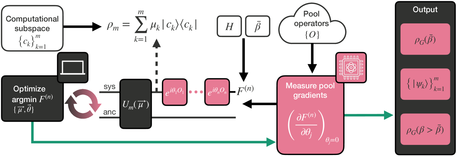
Figure 1: A diagrammatic workflow for TEPID-ADAPT. The white shapes indicate the inputs– the Hamiltonian $H$, the inverse temperature $\bar{\beta}$, an $m$-dimensional computational subspace, and an operator pool for ADAPT. The back circuit, labeled $U_{m}(\vec{\mu})$ is the static part of the ansatz, which prepares $\rho_{m}$ on the system register. The pink circuit parametrized by $\vec{\theta}$ is the adaptively generated portion that maps the computational subspace to the truncated eigenspace of the Hamiltonian. The two solid green arrows (from left-right) respectively indicate the convergence of the VQE subroutine and the pool gradients vanishing. The primary output of TEPID-ADAPT is the target Gibbs state at $\rho_{G}(\bar{\beta})$. We can also prepare the low-lying eigenstates of the Hamiltonian in the truncated subspace $\{\ket{\psi_{k}}\}_{k=1}^{m}$ and the Gibbs states at lower temperatures $\rho_{G}(\beta>\bar{\beta})$.

Variational methods that prepare Gibbs states using other purifications face an obstacle at the level of the cost function. The free energy Eq. (2) is difficult to measure even on quantum hardware because measuring the von Neumann entropy of an arbitrary density matrix requires at least partial state tomography. To get around this difficulty, Ref. [WangPRApp2021] uses a truncated Taylor series of the free energy as the cost function, while Ref. [Warren2022] uses a different cost function that measures proximity to a truncated version of the target Gibbs state. In Ref. [ConsiglioPRA2024], the free energy without any truncation is used as a cost function. This is enabled by a clever modular construction of the parametrized quantum circuit that first prepares a diagonal mixed state on the system qubits, followed by operations that leave the von Neumann entropy invariant. However, the use of a hardware-efficient ansatz for the first block of the circuit and the fact that more ancilla qubits than necessary are used introduce ad hoc elements to the algorithm, additional measurements, and a classical post processing overhead.

In this work, we introduce an algorithm that addresses all these issues simultaneously. Our method uses minimal resources to prepare Gibbs states at low temperatures as well as the low-energy eigenstates that the Gibbs state is primarily composed of. We propose a partially adaptive variational quantum method that uses a parametrized truncation of the Hamiltonian’s spectrum. While the broad modular structure of our ansatz is the same as the one used in Ref. [ConsiglioPRA2024], we use a parametrization in the first (static) part of our ansatz that gives us the von Neumann entropy without the need for classical post-processing. This parametrization also gives us a systematic way to reduce the number of ancillas needed to prepare Gibbs sattes in the low-temperature regime. Once the parametrized mixed state that is diagonal in the computational basis is prepared, we variationally find a unitary with support purely on the system qubits that transforms the state into the truncated eigenbasis of the Hamiltonian. While one could use a static ansatz to do this, we leverage the power of ADAPT-VQE [GrimsleyNatureComm2019], given its ability to find shorter depth circuits. This readily gives us access to the low-lying eigenspectrum of the Hamiltonian, upon successful preparation of the target Gibbs state. This feature also facilitates the preparation of Gibbs states at lower temperatures without any further parameter re-optimization. In Fig. 1, we show a diagrammatic workflow of our method, TEPID-ADAPT.

The organization of the paper is as follows. In Sec. II, we briefly review variational quantum algorithms, with an emphasis on adaptive methods. In Sec. III, we introduce our method TEPID-ADAPT and highlight some of its key features. In Sec. IV, we apply our method to different phases of a standard spin system—the 1D quantum Heisenberg XXZ model—and compare the performance against exact diagonalization. We then conclude in Sec. V, and discuss further directions to pursue.

II Variational quantum algorithms

VQAs have four main ingredients: a parametrized quantum circuit (we will refer to this as the ansatz going forward), a cost function that can be measured on a quantum computer, a reference state, and a classical optimizer that informs the variation of the parameters in the ansatz. For preparing pure states, starting with a computational basis state $\ket{0\cdots 0}\bra{0\cdots 0}$, for instance, is a valid choice because all pure states that are drawn from the same Hilbert space are unitarily equivalent to one-another, which we denote compactly as

$$\ket{\psi_{1}}\bra{\psi_{1}}\stackrel{{\scriptstyle\mathclap{\scriptsize\mbox{$V$}}}}{{=}}\ket{\psi_{2}}\bra{\psi_{2}}.$$ (3)

VQAs aim to solve the optimization problem

$$\vec{\theta}_{c}=\operatorname*{arg\,min}_{\theta}\mathcal{C}(\vec{\theta})\equiv\Tr\left({\mathcal{O}}\,V(\vec{\theta})\ket{\psi_{0}}\bra{\psi_{0}}V^{\dagger}(\vec{\theta})\right),$$ (4)

where $\ket{\psi_{0}}\bra{\psi_{0}}$ is the initial reference state, and ${\mathcal{O}}$ is the operator that is measured to yield the cost function.

The choice of ansatz is an important ingredient in VQAs. A common approach is to use a static ansatz [PeruzzoNature2014, WeckerPRA2015, KandalaNature2017, GardNPJ2020, BurtonPRR2024], where a predefined sequence of parameterized gates are optimized until the convergence criteria are met.

II.1 ADAPT-VQE

Alternatively, one could use an ansatz that is adaptively generated [GrimsleyNatureComm2019, GrimsleyNPJQI2022] using a pool of predefined operators. The operator pool can be tailored for the problem at hand. For instance, a pool could consist of operators that respect some symmetry of the Hamiltonian, or could be comprised of operators related to key interactions in the cost Hamiltonian. The key feature of adaptive VQAs is that the ansatz is not predetermined; it is defined dynamically by adding operators one (or a few) [AnastasiouPRR2024] at a time, each one being chosen based on the local gradients of the pool operators in the cost-function landscape. Measuring these gradients involves some parallelizable overhead on quantum processors. All the parameters are re-optimized after operators are added. This process is repeated until preset convergence criteria are met. This has been shown to be very effective for state preparation for problems in chemistry and physics. Adaptive methods are shown to yield shorter depth circuits [TangPRXQ2021, FeniouSpringerCP2023, AnastasiouPRR2024, Ramoa2024]. They are also resistant to issues associated with difficult optimization landscapes [GrimsleyNPJQI2022, SherbertIEEEConferenceProceeding2024].

When it comes to variationally preparing mixed states, one of the primary challenges is finding the correct unitary equivalence class of the target state $\rho$. This is necessary to guarantee the existence of a unitary acting on the system that connects the reference state $\rho_{0}$ to the target state $\rho$

$$\rho_{0}\stackrel{{\scriptstyle\mathclap{\scriptsize\mbox{$V$}}}}{{=}}\rho\iff\exists\,V:V\rho_{0}V^{\dagger}=\rho.$$ (5)

This challenge is typically addressed by using ancillary qubits and ansätze that span the extended system [CottrellJHEP2019, WuPRL2019, WangPRApp2021, SagastizabalNPJQI2021, Warren2022, ConsiglioPRA2024].

III TEPID-ADAPT

In this section, we introduce our partially adaptive method for variationally preparing low-temperature thermal Gibbs states of a given Hamiltonian. We call our method TEPID-ADAPT, which stands for Truncated Eigenvalue Parametrized Initial Density.

At low temperatures (large $\beta$), only the low-lying energy eigenstates of the Hamiltonian contribute significantly to the Gibbs state. As a result, an approximation of the Gibbs state is

$$\rho_{G}\equiv\frac{e^{-\beta\,H}}{Z}\approx\frac{1}{Z_{m}}\sum_{k=1}^{m}e^{-\beta\,E_{k}}\ket{\psi_{k}}\bra{\psi_{k}},$$ (6)

where $\left\{E_{k},\ket{\psi_{k}}\right\}$ is the ordered eigenspectrum of the Hamiltonian $H$, $m$ is the truncation of the eigenspectrum, and $Z_{m}$ is the truncated partition function. In this work, we treat $m$ as a hyperparameter. $m$ also sets an upper bound on the amount of entanglement between the system and ancillary qubits:

$$S\leq\log m.$$ (7)

Consider the diagonal state in the computational basis

$$\rho_{0}=\frac{1}{Z_{m}}\sum_{k=1}^{m}e^{-\beta\,E_{k}}\ket{c_{k}}\bra{c_{k}},$$ (8)

where $\left\{\ket{c_{k}}\right\}_{k=1}^{m}$ is a set of computational basis elements. We note that $\rho_{0}$ is approximately unitarily equivalent to the Gibbs state

$$\rho_{0}\stackrel{{\scriptstyle\mathclap{\scriptsize\mbox{$V$}}}}{{\approx}}\rho_{G}.$$ (9)

This unitary equivalence would be exact if $m=2^{N}$, where $N$ is the number of system qubits. Inspired by this, we construct a parameterized reference state on the system register that is diagonal in the computational basis with $m$ non-zero eigenvalues:

$$\rho_{m}\equiv\sum_{k=1}^{m}\mu_{k}\ket{c_{k}}\bra{c_{k}},$$ (10)

where the parameters $\{\mu_{k}\}_{k=1}^{m}$ satisfy $\sum_{k=1}^{m}\mu_{k}=1$. With this parametrized $\rho_{m}$ as the reference state, TEPID-ADAPT aims to do two things:

1. Find the correct approximate unitary equivalence class of the target Gibbs state:

   $$\mu_{k}\to\frac{e^{-\beta E_{k}}}{Z_{m}}\quad\forall\,k=1,\cdots,m.$$ (11)

2. Find a unitary operation on the system register that rotates the computational basis to the truncated eigenbasis of $H$:

   $$V_{A}:\ket{c_{k}}\to\ket{\psi_{k}}\quad\forall\,k=1,\cdots,m.$$ (12)

We achieve these using a blocked ansatz shown in Fig 2. The first block $U_{m}(\vec{\mu})$ prepares the parametrized density matrix $\rho_{m}$ in Eq. (10) on the system register. The rest of the ansatz is adaptively generated with support purely on the system register. We denote this block by $V_{A}(\vec{\theta})$ (the subscript stands for adaptive), where $\vec{\theta}$ are the variational parameters of this portion of the ansatz. While we build this unitary adaptively in this work, note that one could instead use a static ansatz. Upon convergence, this becomes a unitary that approximately rotates $\rho_{m}$ to $\rho_{G}$ in Eq. (6). The cost function we use for this VQA is the free energy in Eq. (2). Typically, this is hard to measure because of the difficulty in measuring the von Neumann entropy. In our case, this is made easy by construction of the ansatz: Since $\rho_{m}(\vec{\mu})$ is diagonal in the computational basis, the von Neumann entropy is simply the Shannon entropy:

$$S=-\sum_{k=1}^{m}\mu_{k}\log\mu_{k}.$$ (13)

Moreover, in an instance of the ansatz, $S$ remains unchanged beyond the dashed vertical line in Fig. 2. This is because the $V_{A}(\vec{\theta})$ part of the ansatz only has support on the system register, and the von Neumann entropy of a density matrix is invariant under unitary transformations. Because of this construction, the energy $\langle H\rangle$ is the only piece of the cost function that needs to be measured on the quantum computer, where the cost function is the free energy:

$$F(\vec{\mu},\vec{\theta})=\langle H\rangle(\vec{\mu},\vec{\theta})-\beta^{-1}S(\vec{\mu}).$$ (14)

This makes the measurement complexity in TEPID-ADAPT identical to that of a regular VQE for ground-state preparation. We emphasize here that after the addition of an operator to the ansatz, we re-optimize all the parameters in the ansatz, including the $\vec{\mu}$ parameters. In other words, at each optimization step, both the unitary equivalence class of $\rho_{m}$ and the adaptive unitary $V_{A}$ are allowed to change. The analytical cost function gradients are provided in Appendix LABEL:App:AnalyticalGradients. An example of an explicit construction of $U_{m}$ is provided in Appendix A. The choice of an initial set of parameters $\vec{\mu}$ is addressed in Appendix LABEL:App:InitialState.

[classical gap=0.07cm] $\ket{0}^{\otimes N_{s}}$ N_s [2]U_m(→μ)prep V_A(→θ)$\approx\rho_{G}$
$\ket{0}^{\otimes N_{a}}$ N_a trace

Figure 2: General block diagram for the variational ansatz of TEPID-ADAPT. $U_{m}(\mu)$ prepares $\rho_{m}$ on the system register (top), as indicated by the red line. $V_{A}(\vec{\theta})$ is an adaptively generated unitary on the system register that approximately evolves $\rho_{m}$ to the target Gibbs state.

III.1 Key features

In this section, we highlight two important features of TEPID-ADAPT. Let us denote the adaptive portion of the converged unitary operation by $V_{A}(\vec{\theta}^{*})$ for a given temperature $\bar{\beta}$. Recall that $V_{A}^{\dagger}(\vec{\theta}^{*})$ approximately diagonalizes $H$ in the $m$-truncated subspace. As shown in Fig 2, this unitary acts purely on the system register. The first feature we expand on is how we obtain access to the excited states that contribute significantly to the Gibbs state. To prepare these eigenstates $\{\ket{\psi_{k}}\}$, we simply evolve computational basis states by the converged unitary

$$V_{A}(\vec{\theta}^{*})\ket{c_{k}}\equiv\ket{\psi_{k}}\,\quad\forall\,\,k=1,\cdots,m,$$ (15)

where $\{\ket{c_{k}}\}_{k=1}^{m}$ is the set of computational basis states that we started with in Eq. (10). To find the energies, we can measure the expectation values of the Hamiltonian on the prepared eigenstates:

$$E_{k}=\bra{\psi_{k}}H\ket{\psi_{k}}\,\quad\forall\,\,k=1,\cdots,m.$$ (16)

Alternatively, we can obtain all the energy differences $\Delta E_{k}=E_{k}-E_{0}$ via the ratios of the $\vec{\mu}$ parameters. So, we only need to measure the ground state energy using Eq. (16) to obtain the low-lying energies.

The next feature we highlight is the ability to prepare the Gibbs state at any lower temperature with a fidelity that increases with $\beta$. This feature is a direct consequence of having access to the truncated eigenspectrum. Intuitively, this provides us with the relevant information regarding the interpolation between the Gibbs state at $\bar{\beta}$ and the Gibbs state at $\beta\to\infty$, corresponding to just the ground state. More concretely, we note two things:

1. Excited states become increasingly less important for the Gibbs state as we lower the temperature.

2. $V_{A}^{\dagger}(\vec{\theta}^{*})$ diagonalizes any function of $H$ in the $m$-truncated subspace.

As a result, $V_{A}(\vec{\theta}^{*})$ can be used without any parameter re-optimization to prepare the Gibbs state at any lower temperature $\beta>\bar{\beta}$, provided we prepare the corresponding $\rho_{m}$ first using $U_{m}(\vec{\mu}^{\prime})$, where

$$\mu^{\prime}_{k} =\frac{1}{Z_{m}}e^{-\beta E_{k}}\,\quad\forall\,\,k=1,\cdots,m$$ (17)

$$=\frac{1}{1+\sum_{j=2}^{m}e^{-\beta\Delta E_{j}}}e^{-\beta\Delta E_{j}},$$ (18)

where the energy differences $\Delta E_{j}=E_{j}-E_{1}$ are found using ratios of the $\vec{\mu}$ parameters:

$$\Delta E_{k}=\frac{1}{\beta}\log\frac{\mu_{1}}{\mu_{k}}\,\quad\forall\,\,k=1,\cdots,m.$$ (19)

Moreover, the fidelity with the corresponding Gibbs state improves as we increase $\beta$ because of point 1 above.

IV Results

In this section, we showcase our method TEPID-ADAPT, along with its key features. The results presented here are obtained using noiseless classical simulations. We use the Heisenberg XXZ model with open boundary conditions given by the Hamiltonian

$$H_{\text{XXZ}}=\sum_{k=1}^{N_{s}}\sigma_{k}^{x}\sigma_{k+1}^{x}+\sum_{k=1}^{N_{s}}\sigma_{k}^{y}\sigma_{k+1}^{y}+J_{z}\sum_{k=1}^{N_{s}}\sigma_{k}^{z}\sigma_{k+1}^{z},$$ (20)

where $J_{z}$ is the nearest-neighbor coupling strength of the $ZZ$ interaction, and $\sigma^{x,y,z}$ are the Pauli matrices. This model has ferromagnetic, paramagnetic, and antiferromagnetic phases. This is an integrable model [BetheSprNat1931] and serves as a good test ground for our method. We will present results for parameters corresponding to the three phases. The operator pool we use here to generate the adaptive part of the ansatz, $V_{A}(\vec{\theta})$, is the full Pauli pool, which is the set of all $N_{s}$ qubit Pauli operators, which has size $4^{N_{S}}$. This pool is not scalable to large systems but maximizes the flexibility in the adaptive protocol, so it is appropriate for this proof of concept. In the results below, we consider a system with $N_{s}=6$, and $\bar{\beta}=3.0$.

For each of these phases, we show two figures that compare our results with exact diagonalization:

• Figs. 3, 5, 7 compare the states prepared using TEPID-ADAPT with exact diagonalization for a fixed temperature. We show the infidelity (left axis) and relative errors (right axis) of the energies of the eigenstates in the truncated space, and the free energy of the Gibbs state. The numbered state indices on the horizontal axes of these plots correspond to the eigenstates of the Hamiltonian. These eigenstates are prepared using Eq. (15), and their energies are measured using Eq. (16). The last index $\rho_{G}$ corresponds to the Gibbs state, and its relative error refers to the free energy in Eq. (2). We show results for various values of the cutoff $m$, as indicated by the colors in the legends.

• In Figs. 4, 6, 8, we demonstrate the ability of TEPID-ADAPT to prepare Gibbs states at lower temperatures ($\beta>\bar{\beta}$). We plot the relative free-energy errors of the prepared Gibbs state with the exact one. We run the VQA for $\beta\leq\bar{\beta}$, as indicated by the markers. For $\beta>\bar{\beta}$, we use the same converged adaptive unitary $V_{A}(\vec{\theta}^{*})$ on the system qubits with a modified set of parameters in $U_{m}$, following Eq. (17).

The relative error of a quantity $Q$ is defined as

$$\varepsilon_{\text{rel}}(Q)=\left|\frac{Q-Q_{\text{ex}}}{Q_{\text{ex}}}\right|,$$ (21)

where the subscript ex corresponds to results from exact diagonalization.

The definition of fidelity between two density matrices $\rho,\sigma$ we use in this article is

$$\mathcal{F}(\rho,\sigma)=\left(\Tr\sqrt{\sqrt{\rho}\sigma\sqrt{\rho}}\right)^{2},$$ (22)

which reduces to

$$\mathcal{F}(\ket{\psi},\ket{\phi})=\lvert\bra{\phi}\ket{\psi}\rvert^{2}$$ (23)

for pure states $\ket{\psi},\ket{\phi}$. In the case of degeneracies, we find the fidelity of the prepared state with the degenerate subspace

$$\mathcal{F}\left({\ket{\psi},\{\ket{\phi_{j}}\}_{j=1}^{D}}\right)=\sum_{j=1}^{D}\lvert\bra{\psi}\ket{\phi_{j}}\rvert^{2},$$ (24)

where $\{\ket{\phi_{j}}\}_{j=1}^{D}$ is a set of orthonormal vectors that spans the $D$-degenerate subspace.

In Appendix LABEL:App:Tolerances, we explore the effect of gradient tolerances on the convergence of TEPID-ADAPT. We also include a numerical study of how the cutoff $m$ scales with $N_{s}$ for a given temperature and fidelity threshold for the Heisenberg XXZ model in Appendix LABEL:App:Scaling.

IV.1 Ferromagnetic phase $(J_{z}<-1)$

In the ferromagnetic phase, it is energetically favorable for the spins of the Heisenberg chain to be aligned. As a result, we consider the following computational subspace spanned by states with spins that are fully aligned, or with a low degree of misalignment

$$\left\{c_{k}\right\}\equiv\left\{\ket{000000},\ket{111111},\ket{000001},\ket{111110},\right.\\ \left.\ket{011111},\ket{100000},\ket{001111}\right\}.$$ (25)

In this phase, the ground state is degenerate with a sizable gap. The low-lying eigenspectrum above the degenerate ground state subspace is dense, as shown in the inset of Fig. 3. As a consequence, including a small amount of these states does not significantly improve the fidelity of the Gibbs state, as seen in Fig. 3.

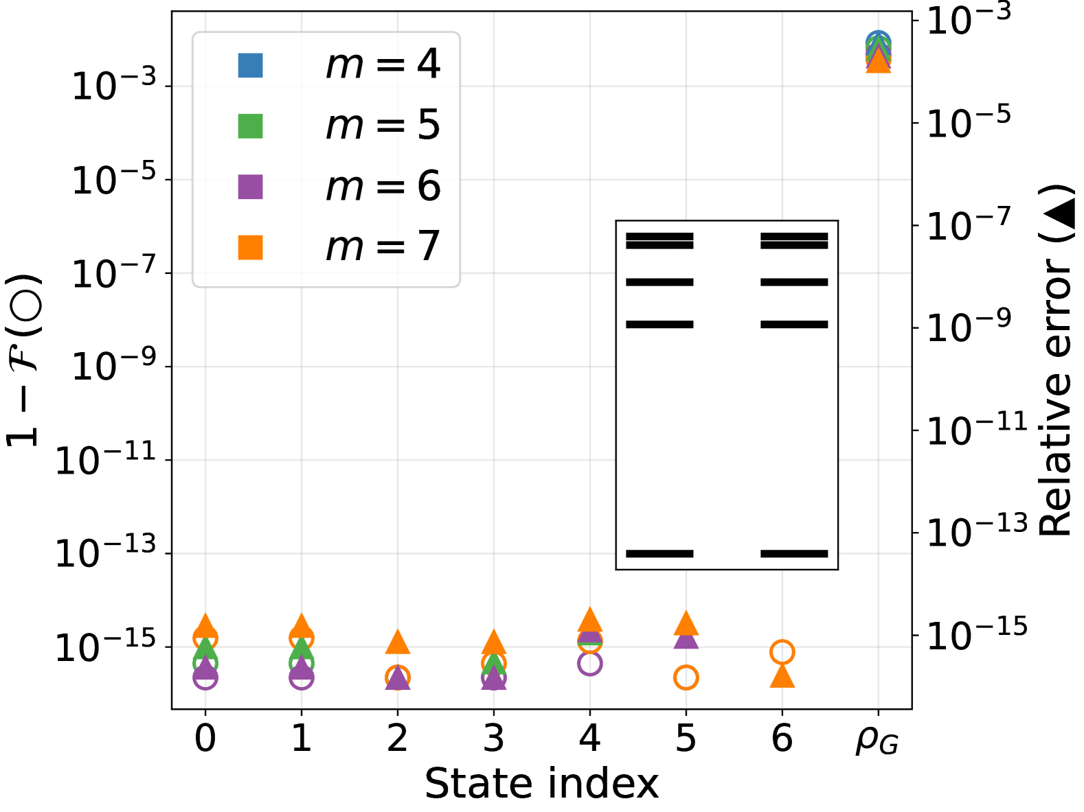
Figure 3: The infidelities (left axis) and relative errors (right axis) of the low-lying eigenenergies, and of the free energy of the $\bar{\beta}=3.0$ Gibbs state of the XXZ model with $N_{s}=6$ and $J_{z}=-1.5$. The numbered state indices refer to the eigenstates, and $\rho_{G}$ to the Gibbs state. The inset shows the low-lying eigenspectrum.

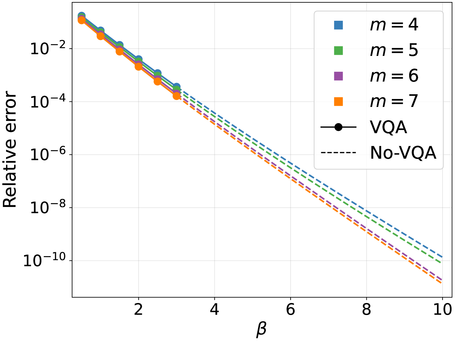
Figure 4: The relative free energy error as a function of $\beta$ for the XXZ model with $N_{s}=6$ and $J_{z}=-1.5$. For $\beta\leq\bar{\beta}$, we prepare the Gibbs state using TEPID-ADAPT, as indicated by the markers. For $\beta>\bar{\beta}$, the same converged adaptive unitary is used with no parameter re-optimization, as indicated by the dashed lines.

IV.2 Paramagnetic phase ($-1<J_{z}<1$)

We have chosen $J_{z}=0$, where the model reduces to the XY spin chain. In the paramagnetic phase, in the absence of an external magnetic field, the spins average to zero net magnetization. As a result, we consider the following computational subspace that includes states with zero or low net magnetization ($M\sim\sum_{j}\langle\sigma^{z}_{j}\rangle$)

$$\left\{c_{k}\right\}\equiv\left\{\ket{010101},\ket{010111},\ket{010100},\ket{100001},\right.\\ \left.\ket{010110},\ket{011110}\right\}.$$ (26)

For $m=4$, we find that the third excited state is not correctly prepared, as seen in Figs. 5, 6. (We find that it instead prepares one of the higher excited states.) However, for larger values of $m$, this is not the case. This emphasizes the need to prepare the Gibbs state using different values of the cutoff $m$ to benchmark the reliability of TEPID-ADAPT in finding the lowest eigenstates. We investigate this in further detail in Appendix LABEL:App:Paramagnetic3state.

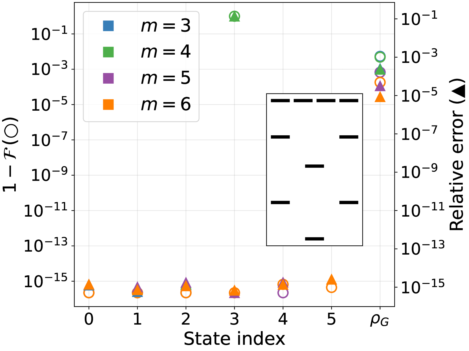
Figure 5: The infidelities (left axis) and relative errors (right axis) of the low-lying eigenenergies, and of the free energy of the $\bar{\beta}=3.0$ Gibbs state of the XXZ model with $N_{s}=6$ and $J_{z}=0.0$. The numbered state indices refer to the eigenstates, and $\rho_{G}$ to the Gibbs state. The inset shows the low-lying eigenspectrum.

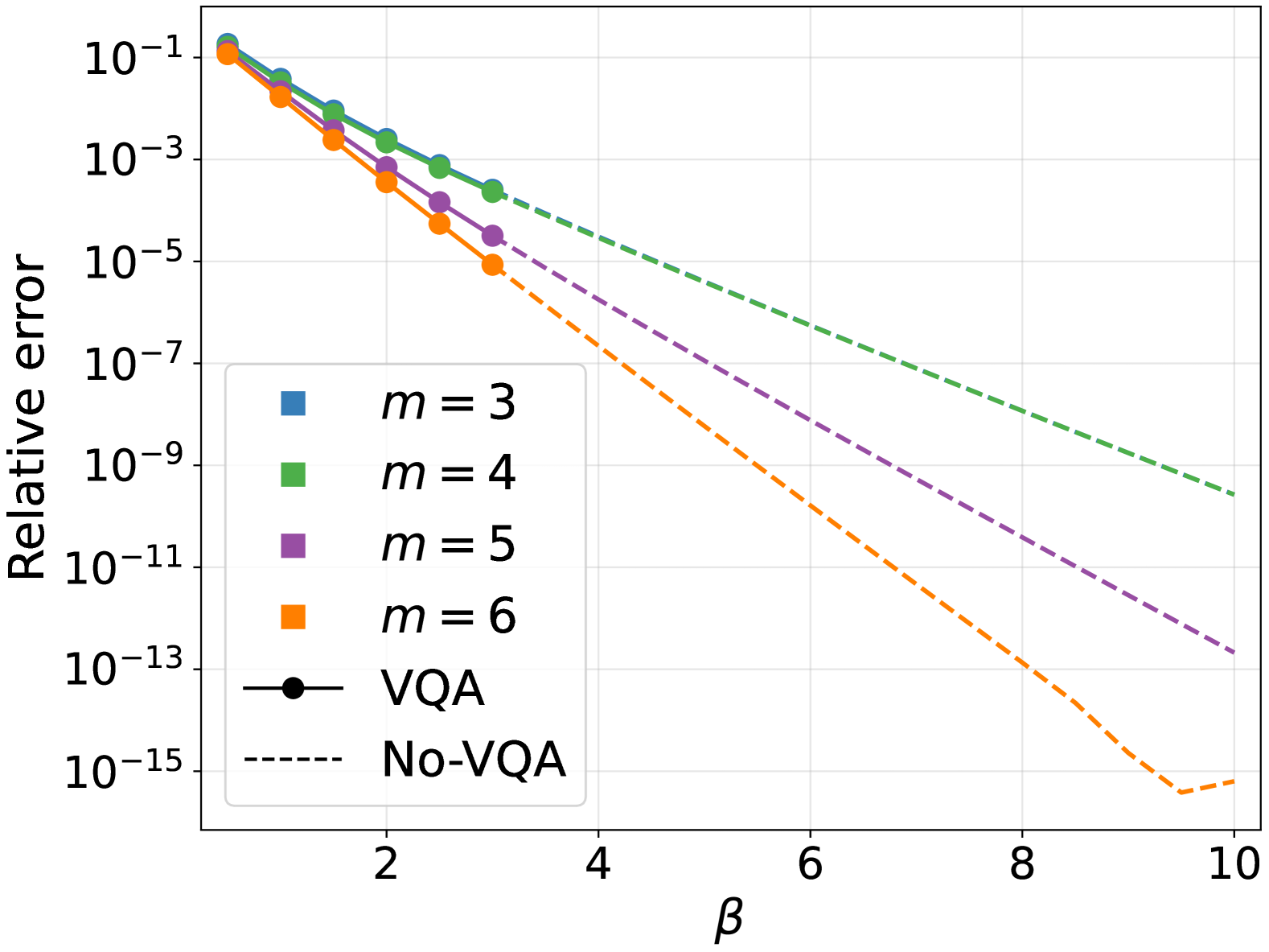
Figure 6: The relative free energy error as a function of $\beta$ for the XXZ model with $N_{s}=6$ and $J_{z}=0.0$. For $\beta\leq\bar{\beta}$, we prepare the Gibbs state using TEPID-ADAPT, as indicated by the markers. For $\beta>\bar{\beta}$, the same converged adaptive unitary is used with no parameter re-optimization, as indicated by the dashed lines.

IV.3 Antiferromagnetic phase ($J_{z}>1$)

In the antiferromagnetic phase, it is energetically favorable for the spins of the Heisenberg chain to be antialigned. As a result, we consider the following computational subspace spanned by states that are either fully, or mostly antialigned

$$\left\{c_{k}\right\}\equiv\left\{\ket{010101},\ket{010110},\ket{010100},\ket{010111},\right.\\ \left.\ket{100101}\right\}.$$ (27)

In this phase, the low-lying eigenspectrum is sparse, as shown in the inset of Fig. 7. This allows us to achieve high fidelities with a relatively small $m$. For $m=5$ in Fig. 7, despite the failure to prepare the fourth excited state, the fidelity of the Gibbs state is high. This shows that this state does not contribute significantly to the Gibbs state at this temperature. This is also evidenced by Fig. 8, where for $\beta\leq 2.0$, the fourth excited state is successfully prepared, indicated by the marginally lower relative free energy error.

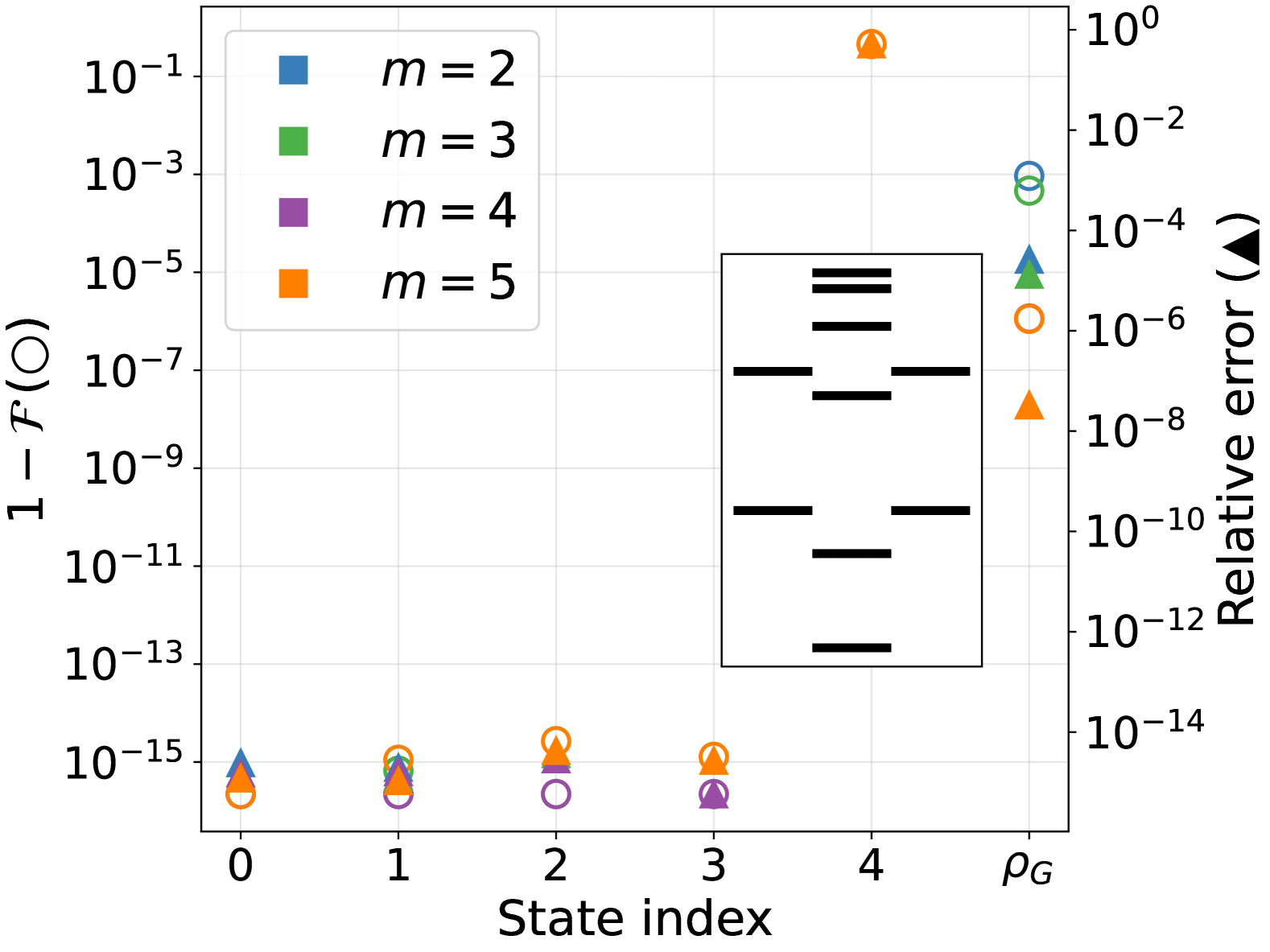
Figure 7: The infidelities (left axis) and relative errors (right axis) of the low-lying eigenenergies, and of the free energy of the $\bar{\beta}=3.0$ Gibbs state of the XXZ model with $N_{s}=6$ and $J_{z}=1.5$. The numbered state indices refer to the eigenstates, and $\rho_{G}$ to the Gibbs state. The inset shows the low-lying eigenspectrum.

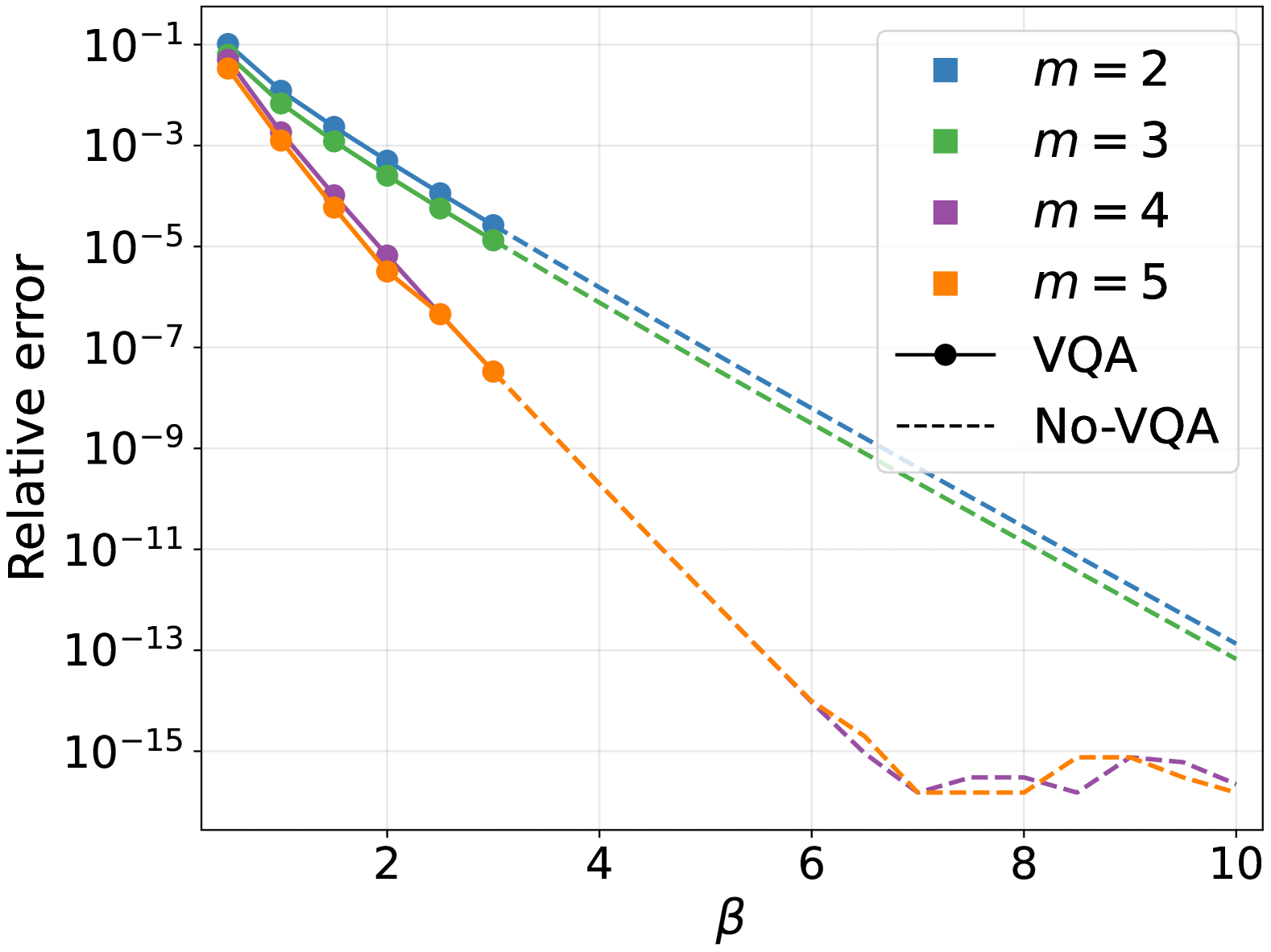
Figure 8: The relative free energy error as a function of $\beta$ for the XXZ model with $N_{s}=6$ and $J_{z}=1.5$. For $\beta\leq\bar{\beta}$, we prepare the Gibbs state using TEPID-ADAPT, as indicated by the markers. For $\beta>\bar{\beta}$, the same converged adaptive unitary is used with no parameter re-optimization, as indicated by the dashed lines.

V Conclusions and outlook

In this article, we introduced TEPID-ADAPT, a variational quantum method to simultaneously prepare low-temperature Gibbs states and the corresponding low-energy eigenstates. We constructed a modular ansatz that is partially static and partially adaptive, and uses a minimal number of ancillary qubits for state purification. The static part spans the extended qubit register, and prepares a parametrized density matrix on the system register. This density matrix is diagonal in the computational basis. The adaptive part of the ansatz has support on only the system register. It aims to find a unitary that rotates the computational basis subspace to the truncated eigenspace, thereby approximately rotating the prepared density matrix to the Gibbs state. This approximation is good at low temperatures, where only the low-lying states contribute significantly to the Gibbs state, provided that the initially chosen computational subspace is large enough.

The nature of the adaptive part of the ansatz grants another nice feature. At temperatures lower than that of the prepared Gibbs state, the excited states become increasingly less important. As a result, we are able to use the same converged adaptive ansatz to prepare lower temperature Gibbs states without any parameter re-optimization. We do have to change the parameters in the static portion of the ansatz appropriately.

A crucial part of VQE is the choice of reference state. This typically has a bearing on the depth of the circuit found to get to the target state. This holds true for TEPID-ADAPT as well – it is important to choose a set of computational basis elements that are effective at finding the low-lying eigenstates that make up the target Gibbs state. In this work, we use system symmetries, and the known phase structure of the Heisenberg XXZ model to make this choice. However, for other models where the choice is less clear, it is important to have a systematic procedure to choose the computational subspace. We save this exploration for future work.

The choice of an operator pool in ADAPT also has a bearing on its effectiveness. In this work, we used the set of all Pauli strings on the system qubits as the pool. The size of this pool scales exponentially in the size of the system. For example, a better choice of an operator pool would take advantage of system symmetries. This has been found to be effective for ground state preparation using ADAPT-VQE [VanDykePRR2024, FarrellPRXQ2024]. We save the analysis of choice of operator pools for TEPID-ADAPT for future work.

In this work, we show how the cutoff $m$ scales with the system size for the Heisenberg XXZ model in Appendix LABEL:App:Scaling. A more general treatment that is less dependent on the particular model at hand is warranted. We save this for future work as well.

Appendix A Explicit form of $U_{m}$

In principle, there are several ways to construct $U_{m}$, using, for example, the quantum channels formalism. The evolution of the system density matrix can be treated as a quantum channel characterized by a set of Kraus operators. One could then find a unitary realization of the channel using ancillary qubits. In this subsection, we provide an intuitive parametrization in terms of a series of Givens rotations (see Eqs. (31), (32)) on the ancillary register, followed by CNOT gates that connect the ancillary and system registers. Finally, we have a permutation matrix on the system register that depends on the choice of the computational subspace. Note that this likely is not the most efficient way to implement $U_{m}$, but serves as an example. For this form of $U_{m}$, we require a minimal number of ancillary qubits $N_{a}=\lceil{\log_{2}m}\rceil$.

First, we write down a re-parametrization of $\vec{\mu}$ in terms of angles, using the $m$-dimensional spherical polar coordinates

$$\sqrt{\mu_{j}}=\begin{cases}\left(\prod_{k=1}^{j-1}\sin(\varphi_{k})\right)\cos(\varphi_{j})&1\leq j<m\\ \\ \left(\prod_{k=1}^{m-1}\sin(\varphi_{k})\right)&j=m\end{cases},$$ (28)

where $m$ is the number of parameters, corresponding to the number of non-zero eigenvalues in $\rho_{m}$. This re-parametrization maps the $m$ parameters $\vec{\mu}$, with the unit trace constraint to $m-1$ independent angles $\vec{\varphi}$. It also ensures the positivity of $\vec{\mu}$.

Next, we prepare on the ancillary register the pure state

$$\ket{\xi}=\sum_{k=1}^{m}\sqrt{\mu_{k}}\ket{k-1},$$ (29)

where $\{\ket{k}\}$ are the computational basis elements. For instance, $\ket{3}$ on a 4-qubit ancillary register corresponds to $\ket{0011}$. This is done using a series of $m-1$ Givens rotations

$$\ket{\xi}=\prod_{k=1}^{m-1}G^{(k,k+1)}(\varphi_{k})\ket{0}^{\otimes N_{a}},$$ (30)

where $G^{(k,k+1)}(\varphi_{k})$ is the Givens rotation generated by the exponential map

$$G^{(k,k+1)}(\varphi_{k})\equiv\exp\left({i\,\varphi_{k}\gamma^{(k,k+1)}}\right),$$ (31)

where the matrix elements of $\gamma^{(k,k+1)}$ are

$$\left[\gamma^{(k,k+1)}\right]_{x,y}=i\left(\delta_{x,k}\,\delta_{y,k+1}-\delta_{x,k+1}\,\delta_{y,k}\right),$$ (32)

using $\delta_{i,j}$ for the Kronecker delta. Geometrically, this corresponds to an $SO(2^{\lceil\log_{2}m\rceil})$ rotation from

$$\left(1,0,\cdots,0\right)\to\left(\sqrt{\mu_{1}},\cdots,\sqrt{\mu_{m}},\cdots\right),$$ (33)

where the vectors are in the computational basis. The last set of $\cdots$ on the second vector corresponds to a padding with $2^{\lceil\log_{2}m\rceil}-m$ zeros.

A.1 Intuitive implementation

Following this, we perform a set of CNOT operations with the $j^{th}$ ancillary qubit as the control, and the $(N_{s}-m+j)^{th}$ system qubit as the target, for every ancillary qubit. Note that this is a single layer of CNOT gates. The state on the system + ancillary register after this operation is

$$\ket{\Omega(\vec{\varphi})}=\sum_{k=1}^{m}\sqrt{\mu_{k}}(\vec{\varphi})\left(\ket{k-1}\otimes\ket{k-1}\right),$$ (34)

where the ordering of the tensor product is (system $\otimes$ ancilla). The next step is the application of a permutation matrix on the system register. These are a class of matrices that permute the computational basis. The particular permutation matrix $P\left(\left\{\ket{c_{k}}\right\}\right)$ we need is the one that maps the first $m$ computational basis elements $\left\{\ket{k-1}\right\}_{k=1}^{m}$ to the chosen computational subspace $\left\{\ket{c_{k}}\right\}_{k=1}^{m}$ giving us the state

$$\ket{\Phi(\vec{\varphi})}=\sum_{k=1}^{m}\sqrt{\mu_{k}}(\vec{\varphi})\left(\ket{c_{k}}\otimes\ket{k-1}\right),$$ (35)

Then, upon tracing out the ancillary qubits, we obtain

$$\Tr_{a}\ket{\Phi(\vec{\varphi})}\bra{\Phi(\vec{\varphi})}=\sum_{k=1}^{m}\mu_{k}(\vec{\varphi})\ket{c_{k}}\bra{c_{k}}\equiv\rho_{m}$$ (36)

on the system register, as needed. An illustrative example of the circuit of $U_{3}$ using the above construction for a system with three qubits is shown in Fig. LABEL:fig:GivensAnsatz. Upon tracing out the ancillary qubits, one obtains the desired $\rho_{3}$ on the system register, as indicated.

The scalability of the specific type of permutation matrices we use here with $N_{s}$ is unclear. We use this construction as an intuitive example. We could instead use $m$ multi-controlled gates with the ancillary register as the controls and the system register as the targets to map to the desired $N_{s}$ qubit computational basis subspace. We discuss this realization along with its scalability below.

[classical gap=0.07cm] $s_{1}$ [3]P(