What’s the matter with $\Sigma m_{\nu}$?

Abstract

Due to non-zero neutrino rest masses we expect the energy density today in non-relativistic matter, $\omega_{\rm m}$, to be greater than the sum of baryon and cold dark matter densities, $\omega_{\rm cb}$. We also expect the amplitude of deflections of CMB photons due to gravitational lensing to be suppressed relative to expectations assuming massless neutrinos. The combination of CMB and BAO data, however, appear to be defying both of these expectations. Here we review how the neutrino rest mass is determined from cosmological observations, and emphasize the complementary roles played by BAO and lensing data in this process. We explain why, for current constraints on the sum of neutrino masses, the addition of BAO data to primary CMB data is much more informative than the addition of CMB lensing reconstruction data. We then use a phenomenological model to find that the preference from CMB and BAO data for a matter density that is below expectations from the CMB alone is at the $3\,\sigma$ level. We also show that if a fraction of the dark matter decays to dark radiation, the preference for $\omega_{\rm m}>\omega_{\rm cb}$ can be restored, but with a small increase to the CMB lensing excess.

I Introduction

The standard Big Bang model predicts a sea of relic neutrinos that decoupled at $T\sim 1\text{ MeV}$. The contribution of this neutrino background to the overall energy density has been detected using precise measurements of the cosmic microwave background (CMB), and is consistent with the presence of three massless neutrino species [1, 2, 3, 4]. Neutrinos are known to have mass, however, from atmospheric and solar neutrino oscillation observations, with a sum of neutrino masses $\Sigma m_{\nu}$ that must exceed about 0.06 eV [5]. Current upper limits from cosmological observations are approaching this bound [6, 7, 8, 4, 9]. A clear detection of $\Sigma m_{\nu}$ from cosmological observations may occur in the near future and would constitute a milestone in both cosmology and particle physics [10].

However, not only has such a detection not yet occurred, but two different features of the data have emerged which are surprisingly opposite to what one would expect as signatures of neutrino mass. The first is that the reconstructed lensing power from Planck [11], the Atacama Cosmology Telescope (ACT) [12], and SPT-3G [4] is higher than expectations from Planck primary CMB and DESI baryon acoustic oscillation (BAO) data, assuming $\Lambda$CDM. As demonstrated in Ge et al. [4], this preference for excess lensing power holds regardless of which Planck likelihood is used, and regardless of which lensing reconstruction is used. By artificially scaling the lensing amplitude with a parameter $A_{\rm lens}$, they found that the combination of Planck primary CMB, BAO, and all three of the aforementioned lensing reconstructions favors [4]

$$A_{\rm lens}=1.083\pm 0.032,$$ (1)

a $2.7\,\sigma$ detection of excess lensing power.

Another phenomenological model for quantifying this excess lensing power was introduced earlier in 2024 by [13] and subsequently studied in [14]. Instead of $A_{\rm lens}$ they introduced a neutrino-mass-like parameter, $\Sigma\tilde{m}_{\nu}$, that controls a template for adjusting the model CMB lensing power. For negative values of $\Sigma\tilde{m}_{\nu}$ lensing power is enhanced, to the same degree as the suppression caused by $\mbox{$\Sigma m_{\nu}$}=|\Sigma\tilde{m}_{\nu}|$. They found $\Sigma\tilde{m}_{\nu}<0$ at $2.4\,\sigma$. Other effective neutrino mass parameterizations have found consistent results [15].

In this paper, we discuss and quantify the second line of evidence. Allowing for the possibility that the comoving density of non-relativistic matter can decrease after recombination, we show that this scenario is in fact favored by CMB and BAO data. This is also the opposite of what is expected from massive neutrinos: since they become non-relativistic after recombination, we expect them to contribute to the total physical matter density today, $\omega_{\rm m}$. That the interaction of BAO and CMB constraints on the background evolution prefers $\omega_{\rm m}<\omega_{\rm cb}$ (where $\omega_{\rm cb}$ is the density of baryons and cold dark matter) was explained by Loverde and Weiner [16], but not quantified. We do so here by phenomenologically extending the effect of neutrino masses on the background expansion to negative values. Using Planck PR3 primary CMB data and BAO data from SDSS and DESI, we find a $3\,\sigma$ preference for $\omega_{\rm m}$ being less than expected from CMB data alone (assuming $\mbox{$\Sigma m_{\nu}$}=0.06\,{\rm eV}$). We refer to this as a “matter-density deficit.”

In this paper, we also consider the complementary roles played by CMB lensing data and BAO data regarding constraints on neutrino mass. Understanding how constraints from these data sets interact is useful in clarifying how each contribute to current bounds on the neutrino mass. In considering these data sets, we find that BAO data are much more informative than CMB lensing reconstruction data, when combined with measurements of the primary CMB power spectra, and explain why.

The origin of these observational signatures (the matter-density deficit, and the CMB lensing power excess) is unclear, as is whether or not they share a common origin. It is possible that a single model could explain both features, or that they are resolved separately. We work out an example, involving decaying dark matter along with a free neutrino mass, that explains the $\omega_{\rm m}<\omega_{\rm cb}$ preference, but without addressing the excess lensing problem. Until these features of the data are better understood, current tight limits, derived under the assumption of the $\mbox{$\Lambda$CDM}+\mbox{$\Sigma m_{\nu}$}$ model, should be interpreted with care.

We are submitting this paper nearly simultaneously with new CMB and BAO releases from the ACT, SPT, and DESI Collaborations. Our analyses will change quantitatively when we incorporate these new data, and we are quite eager to see whether there will be any qualitative change, such as new clues as to how the discrepancies might be resolved. We hope that our work will be helpful to those trying to understand the implications of these new data.

This paper is organized as follows. In Section II we review how CMB and BAO data can constrain neutrino masses, both separately and in conjunction. In Section III.1 we introduce our effective neutrino mass model, discuss our analysis methodology, and present constraints in this model showing a background preference for a matter-density deficit. We then introduce a DDM model in Section IV which is similar to the effective neutrino mass model at the background level, and discuss the constraints in this model space. We briefly review possible solutions to these problems in Section V, before concluding in Section VI.

II Review of constraints on the neutrino mass

With this section we aim to provide the reader with a conceptual understanding of how cosmological observations, CMB and BAO in particular, enable constraints on the neutrino mass. These observables are sensitive to the gravitational influence of massive neutrinos, which fundamentally makes these constraints possible. For neutrinos in mass ranges of interest, which become non-relativistic after recombination, a combination of probes is necessary to isolate this influence.

The measurement of $\Sigma m_{\nu}$ from cosmological data can be thought of as proceeding in two steps. First, the CMB temperature and polarization power spectra are used to estimate the baryon and cold dark matter densities, along with the angular size of the sound horizon; together, these give a constraint on the distance to the last-scattering surface. Knowing this distance is not sufficient to determine $\Sigma m_{\nu}$, as we can simultaneously vary the cosmological constant and $\Sigma m_{\nu}$ to keep that distance fixed, but with slightly different shapes for the expansion history. To break the degeneracy we can then either add BAO data, which (in combination with the primary CMB data) constrain $\omega_{\rm m}=\omega_{\rm cb}+\omega_{\nu}$, or CMB lensing data, which constrains a different linear combination that is approximately $\omega_{\rm cb}-0.5\omega_{\nu}$. Of course, one can also add both for even greater constraining power. We explain these steps in detail in the remainder of this section.

II.1 Primary CMB

First we discuss how the mass/energy densities in the various components of the $\Lambda$CDM model can be determined from CMB data if one assumes the $\Lambda$CDM model, before moving on to the case of the $\Lambda$CDM model extended to include an unknown spectrum of neutrino masses.

II.1.1 Component densities determined assuming $\Lambda$CDM and ignoring CMB lensing

In $\Lambda$CDM the energy density in relativistic particles (radiation density) is completely determined by the FIRAS determination of the CMB temperature [17] and assumptions relevant to the thermal production of three species of neutrinos. To be concrete, for now we will assume three species of massless neutrino, so that all of their energy is included in the radiation density. The remainder of the mass/energy density is controlled by three parameters which we can take to be the energy densities today of baryons, $\omega_{\rm b}$, and cold dark matter, $\omega_{\rm c}$, and the angular size of the sound horizon at the epoch of recombination, $\theta_{s}^{\star}$. The other $\Lambda$CDM parameters describe the spectrum of primordial fluctuations ($A_{s}$ and $n_{s}$) and the reionization history, $\tau_{\rm reio}$.

All three of these quantities ($\omega_{\rm b}$, $\omega_{\rm c}$, $\theta_{\rm s}^{*}$) can be determined with a high degree of precision from CMB temperature anisotropies, polarization anisotropies, or the combination with very little (although some, as we will explore) sensitivity to potential departures from $\Lambda$CDM in the post-recombination universe. For a discussion of the physics that allows one to infer $\omega_{\rm c}$, $\omega_{\rm b}$, and $\theta_{s}^{\star}$ (as well as the other three $\Lambda$CDM parameters) from CMB anisotropy data, see Aghanim et al. [18].

Obviously $\theta_{s}^{\star}$ is not a density, but given the other two and the $\Lambda$CDM model, the dark energy density can be inferred, as we now explain. The angular size of the sound horizon is the angle subtended by the sound horizon, projected from the last-scattering surface. It is thus given by $\theta_{s}^{\star}=r_{s}^{\star}/D_{A}^{\star}$ where $r_{s}^{\star}$ is the comoving size of the sound horizon at last scattering and $D_{A}^{\star}$ is the comoving angular-diameter distance to last scattering. These depend on the expansion rate and sound speed in the plasma via:

$$r_{s}^{\star}=\int_{z_{\star}}^{\infty}\frac{c_{s}(z)}{H(z)}\differential z\mbox{\quad and\quad}D_{A}^{\star}=\int_{0}^{z_{\star}}\frac{c}{H(z)}\differential z$$ (2)

where $z_{\star}$ is the redshift of recombination, which for the standard recombination scenario is around $z_{\star}\approx 1090$. The expansion rate prior to recombination, via the Friedmann equation, depends only on the baryon, cold dark matter, and radiation densities, as the cosmological constant contribution is negligibly small. Additionally, of the $\Lambda$CDM parameters, $\omega_{\rm b}$ and $\omega_{\rm c}$ are all that is needed to determine $z_{\star}$ and $r_{s}^{\star}$. Given $\theta_{s}^{\star}$, $\omega_{\rm b}$, and $\omega_{\rm c}$ one can thus determine $D_{A}^{\star}=r_{s}^{\star}/\theta_{s}^{\star}$. The only unknown density in the integrand for calculating $D_{A}^{\star}$ is $\omega_{\Lambda}$, and thus one can determine it. With $\omega_{\Lambda}$ determined in this way, $H(z)$ is also known at all redshifts. See [e.g. 19] for more details.

II.1.2 Component densities determined assuming $\Lambda$CDM + free $\Sigma m_{\nu}$

The previous section modeled neutrinos as massless particles; however, from observations of solar and atmospheric neutrinos it is known that at least two neutrino species have non-zero mass. Current global analyses of neutrino oscillation data have constrained the squared mass differences to be $\Delta m^{2}_{21}\approx 7.5\times 10^{-5}{\rm\ eV}^{2}$ and $|\Delta m^{2}_{31}|\approx 2.55\times 10^{-3}{\rm\ eV}^{2}$ [20, 21]. Depending on the sign of $\Delta m^{2}_{31}$, these constraints set lower bounds for the sum of the masses: in the normal ordering (i.e. $m_{3}>m_{1}$, hereafter NO) we have $\mbox{$\Sigma m_{\nu}$}>0.06{\rm\ eV}$, and in the inverted ordering (IO), $\mbox{$\Sigma m_{\nu}$}>0.1{\rm\ eV}$. Because near-term cosmological data will not measure individual masses [22], the cosmological impact of neutrino mass is usually parameterized by the sum of their masses, $\Sigma m_{\nu}$.

Freeing $\Sigma m_{\nu}$ changes the picture described previously in two ways. First, the post-recombination total energy density, and thus expansion rate, now depends both on $\omega_{\Lambda}$ and on the unknown neutrino density. Given just $\theta_{s}^{\star}$, $\omega_{\rm b}$, and $\omega_{\rm c}$ there is now a degeneracy between $\omega_{\Lambda}$ and $\Sigma m_{\nu}$, so $H(z)$ is no longer completely determined. Instead, we have a one-parameter family of $H(z)$ curves which all give the same $D_{A}^{\star}$ and therefore $\theta_{s}^{\star}$. Some members of this family are shown in Fig. 1.

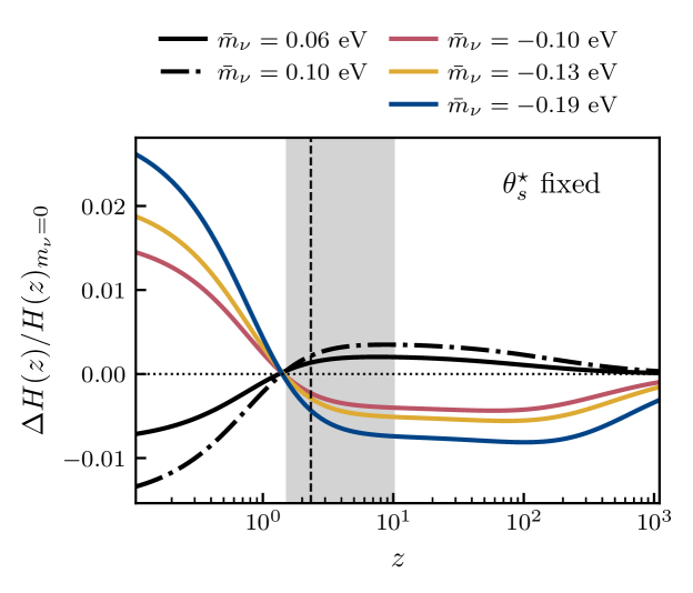
Figure 1: Similar to Fig. 1 of Pan and Knox [23] we show here fractional changes to the expansion rate at fixed angular size of the sound horizon, as projected from the last-scattering surface. The baseline expansion rate is for a model with $\mbox{$\Sigma m_{\nu}$}=0$. The $\bar{m}_{\nu}$ parameter and the associated phenomenological model are described in Section III.1 — positive values of $\bar{m}_{\nu}$ are identical to physical neutrinos with $\mbox{$\Sigma m_{\nu}$}=\bar{m}_{\nu}$ at the background level. The gray band indicates the full width at half maximum of the CMB lensing kernel, showing the redshifts to which CMB lensing is most sensitive. The vertical dashed line is at $z=2.33$, the maximum redshift for which we include BAO measurements.

A second way neutrino masses can alter the picture presented so far arises when neutrinos become non-relativistic around or before recombination. Defining the transition to non-relativistic to occur when the rest mass is comparable to the average kinetic energy we get

$$1+z_{\rm nr}=\frac{m_{\nu}}{3.15T_{\nu 0}}\approx 113\frac{m_{\nu}}{0.06\text{ eV}}.$$ (3)

This transition occurs near recombination or earlier for neutrinos more massive than $m_{\nu}\sim 0.6\ {\rm eV}$. Masses in this range will lead to changes in early ISW effects, providing a new CMB signal (beyond what is captured by $\omega_{\rm b}$, $\omega_{\rm c}$, and $\theta_{s}^{\star}$ inferences) allowing for the degeneracy between $\omega_{\Lambda}$ and $\Sigma m_{\nu}$ to be partially broken [24, 25]. We do not elaborate further on this degeneracy breaking since the addition of any of CMB lensing, BAO, or uncalibrated supernova measurements constrains neutrino masses sufficiently tightly that the alterations of early ISW effects are negligible.

II.2 CMB Lensing

As CMB photons travel from the last-scattering surface, their paths are distorted by gravitational potential gradients perpendicular to their momenta. Gradients in the resulting deflections lead to shearing, magnification, and demagnification of the otherwise statistically isotropic and Gaussian patterns of anisotropy. One can use the resulting departures from statistical isotropy to infer convergence maps and therefore the CMB lensing deflection power spectrum [26, 27, 28, 29]. CMB lensing information is also contained in CMB power spectra inferred from the observed lensed maps. Since they are derived from both magnified regions in which angular spectral patterns are shifted to lower $\ell$, and demagnified regions with shifts to higher $\ell$, the acoustic features in the map are smeared, and the drop of power toward high $\ell$ caused by Silk damping is softened [30].

That CMB measurements alone, including CMB lensing, can allow for tight constraints on $\Sigma m_{\nu}$, with errors comparable to the minimum value of 0.06 eV, was first pointed out by Kaplinghat et al. [31]. The impact of neutrino mass on CMB lensing is best explained with reference to Fig. 1. Increasing $\Sigma m_{\nu}$ leads to an increased expansion rate at $z\gtrsim 1$ which slows down growth on scales below the neutrino free-streaming length, as a faster expansion rate inhibits the transport of matter from underdense regions to overdense regions. Increasing mass also decreases the neutrino free-streaming length; on scales above the free-streaming length the suppressive effect of the faster expansion is mitigated by the clustering of the neutrinos themselves, as they source large-scale gravitational potentials. The suppression of growth at $z\gtrsim 1$ leads to a suppression of the matter power spectrum today and of the CMB lensing power spectrum, on scales below the neutrino free-streaming length.

When only considering CMB power spectra, the lensing-induced peak smearing is the dominant effect contributing to neutrino mass bounds, and makes CMB data sensitive to neutrinos less massive than $m_{\nu}<0.6\text{ eV}$. Lensing allows one to break the background-level degeneracy with $\omega_{\Lambda}$ and place constraints on $\Sigma m_{\nu}$ with only CMB data. However, it also means that inferences of $\Sigma m_{\nu}$ are sensitive to anything that impacts the lensing inference, in particular the well-known $A_{\rm 2pt}$ (or, $A_{L}$) anomaly in Planck PR3 data [1]. Indeed, as noted by many authors [e.g. 32, 33, 14, 34], the $A_{\rm 2pt}$ anomaly contributes to the tight bounds on $\Sigma m_{\nu}$ from Planck data, because the reduction in lensing stemming from positive $\Sigma m_{\nu}$ results in a “peak sharpening” that is out of phase with the oscillatory residuals in PR3 data, within $\Lambda$CDM, that resemble peak smearing.

We highlight a related point, which is that CMB lensing power is also highly sensitive to $\omega_{\rm cb}$ [35]. As such, lensing features in the CMB power spectra, or the reconstructed CMB lensing data itself, can influence inference of $\omega_{\rm cb}$. Lensing power increases with increasing $\omega_{\rm cb}$, mainly due to the higher matter-to-radiation density ratio when a perturbation mode of a given wavelength crosses the horizon. The greater this ratio, the less gravitational potential decay occurs. In the $\Lambda$CDM model, the final constraint on $\omega_{\rm cb}$ is a balance between fitting early universe effects (such as radiation driving and the associated boost in power), and this lensing-related effect impacting the CMB at later times. When $A_{\rm 2pt}$ is marginalized over, so that the lensing information in the CMB power spectra is effectively lost, the dark matter density inferred from the Planck PR3 data is lowered [1]. We will return to this fact, and its relevance to our findings, in Section III.3.

II.3 BAO

The sound horizon is also imprinted on the distribution of matter, and therefore the galaxy distribution. Using data from galaxy surveys, it is possible to infer

$$\theta_{s}(z)=r_{\rm d}D_{A}(z)\text{ and }\Delta z_{s}=r_{\rm d}dH(z)$$ (4)

which correspond to the sound horizon scale in the transverse and line-of-sight directions [e.g. 36, 37, 38, 39]. Here, $r_{\rm d}$, is the sound horizon at the baryon drag epoch. In the $\Lambda$CDM model, even with extension to free $\Sigma m_{\nu}$, constraints on these parameters at multiple redshifts can be compressed losslessly into just two constraints. One is typically taken to be $\Omega_{\rm m}$, which completely controls the (un-normalized) shape of both $H(z)$ and $D_{A}(z)$. Here, $\Omega_{\rm m}$ is the present fraction of the energy density in non-relativistic matter, including the neutrino rest-mass density. The other is typically a constraint on $r_{\rm d}h$, where $H_{0}=100\ h$ km/sec/Mpc. This second parameter pins down the normalizations allowing one to relate the un-normalized $H(z)$ (specified by $\Omega_{\rm m})$ to both $\theta_{s}(z)$ and $r_{\rm d}H(z)$.

Inference of the physical matter density $\omega_{\rm m}$, instead of $\Omega_{\rm m}$, would be much more valuable in terms of determining the neutrino mass because it could be directly compared to the CMB-inferred $\omega_{\rm cb}$, with any difference attributable to the neutrinos. For this reason, the reparameterization from ($\Omega_{\rm m}$, $r_{\rm d}h$) to ($\Omega_{\rm m}$, $\omega_{\rm m}r_{\rm d}^{2}$) has a significant advantage for understanding the impact of BAO constraints on $\Sigma m_{\nu}$ – particularly when combined with CMB constraints [16]. Given some fiducial $\omega_{\rm b}$ and $\omega_{\rm c}$, one can then calculate $r_{\rm s}$ and then transform $\omega_{m}r_{\rm d}^{2}$ to

$$\mbox{$\Sigma m_{\nu}$}=\frac{\omega_{\rm m}r_{\rm d}^{2}-\omega_{\rm cb,f}r_{\rm d,f}^{2}}{r_{\rm d,f}^{2}}\times 93.14\ {\rm eV}$$ (5)

since $\omega_{\rm m}=\omega_{\nu}+\omega_{\rm cb}$ and $\mbox{$\Sigma m_{\nu}$}=\omega_{\nu}\times$ 93.14 eV. This transformation is, in a sense, comparing the matter density today of constituents that were non-relativistic prior to recombination, as inferred from CMB data, to the matter density inferred from BAO observations, after CMB calibration of $r_{\rm d}$. In Section III, we will use a similar (but subtly different) approach.

By comparing the constraints from the CMB BAO angle $\theta_{s}^{\star}$ and the galaxy survey BAO constraints (as inferred from both DESI and SDSS) in this plane, Loverde and Weiner [16] found that they overlap primarily at values of $\omega_{\rm m}r_{\rm d}^{2}$ that are less than the best-fit $\omega_{\rm cb}r_{\rm d}^{2}$ as inferred from Planck CMB data. (See their Fig. 3 and/or our Fig. 5). This is, of course, the opposite of what one would expect given $\mbox{$\Sigma m_{\nu}$}>0$.

II.4 Complementary Roles of BAO and CMB Lensing

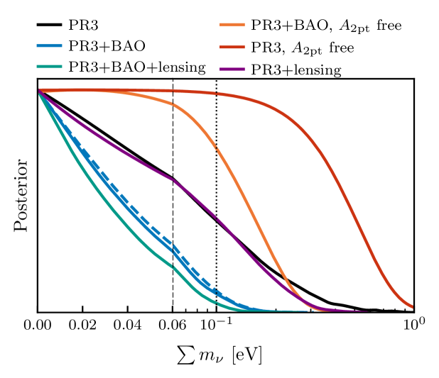
Figure 2: Constraints on $\Sigma m_{\nu}$ from different datasets, which are described in Table 1. The blue dashed line is the constraint one obtains from our effective neutrino mass model and background-only likelihoods (both described in Section III) with a prior $\bar{m}_{\nu}\geq 0$ eV. The CMB information about $\Sigma m_{\nu}$ can therefore be mostly encapsulated by the background-only likelihoods.

Loverde and Weiner [16] emphasize the importance of this comparison between $\omega_{\rm m}r_{\rm d}^{2}$ with $\omega_{\rm cb}r_{\rm d}^{2}$, along the constraint provided by the CMB determination of $\theta_{s}^{\star}$. They claim it is the dominant source of information about $\Sigma m_{\nu}$ from current data. Because of the importance of distance-redshift relations to inferring $\Sigma m_{\nu}$ in this manner, they refer to this information as “geometrical.” They perform an analysis of Planck PR3 power spectra + BAO data in which $A_{\rm 2pt}$ is allowed to be free, and refer to the results as “geometrical constraints.” The resulting constraints in the $\Omega_{\rm m}-\omega_{\rm m}r_{\rm d}^{2}$ plane are indeed quite similar to what one would expect from their analysis in this plane using fixed fiducial values of the CMB-derived parameters $\omega_{\rm b}$, $\omega_{\rm c}$, and $r_{\rm s}$.

This emphasis on geometry is in contrast to the emphasis on CMB lensing as a source of the neutrino-mass constraint in [13] and [14]. Motivated by the fact that measured CMB lensing is a bit high compared to $\Lambda$CDM expectations, which is opposite to the effect expected from $\mbox{$\Sigma m_{\nu}$}>0$, these authors performed an analysis with a phenomenological model that continued those lensing power effects into negative values of an effective neutrino mass parameter, $\tilde{m}_{\nu}$. They found, on the basis of the observed excess lensing, a preference for $\Sigma\tilde{m}_{\nu}<0$ at $2.4\,\sigma$ significance.

Excess CMB lensing power was also subsequently studied in Ge et al. [4]. Rather than a neutrino-mass-inspired lensing power template as used by Craig et al. [13], they simply extended the $\Lambda$CDM model with $A_{\rm lens}$, a parameter that simply multiplies the $\Lambda$CDM model lensing power used for comparison to lensing power reconstructions and for calculating model temperature and polarization power spectra (TT/TE/EE). They found a preference for excess lensing power for a variety of dataset combinations, with and without BAO, and with either PR3 or PR4 TT/TE/EE. Preferences ranged, for cases in which all CMB lensing reconstruction data were used, from as small as $1.7,\sigma$ (without BAO and with PR4 TT/TE/EE) to $2.7\,\sigma$ (with BAO and PR3 TT/TE/EE).

We now turn to the relationship between BAO and CMB lensing as probes of neutrino mass, beginning with a misconception. It is sometimes claimed that the main role of BAO data is in tightening the primary CMB-based predictions for the lensing amplitude, mainly through sharpening constraints on $\omega_{\rm c}$, so that any suppression (or enhancement) can be clearly detected [e.g. 40]. While this does indeed happen in the case that lensing and BAO data are used jointly, we see in Fig. 2 that adding BAO data to primary CMB data leads to significantly tighter $\Sigma m_{\nu}$ constraints regardless of how CMB lensing is treated. Clearly, BAO data cannot be purely a means to make better use of CMB lensing information.

This misconception may have arisen because the impact of neutrino mass on the density of non-relativistic matter is so small. It is indeed small, but as explained by Loverde and Weiner [16] the interaction with $\theta_{s}^{\star}$ magnifies its importance, as can also be seen in Fig. 1 of Pan and Knox [23]. If one varies the expansion rate in a manner that keeps $\theta_{s}^{\star}$ fixed (or at high CMB likelihood), the tiny contribution to the expansion rate from $\Sigma m_{\nu}$, because it persists over so much comoving distance on our past light cone, gets amplified: the cosmological constant has to make up for it over a much smaller co-moving distance. The low-redshift feature to which the BAO data are sensitive is best fit in $\Lambda$CDM (at the $\theta_{s}^{\star}$ value preferred by Planck) via a high value of the cosmological constant, which is equivalent to a much more moderate decrease to the value of the matter density. It is this increase to the cosmological constant (with $\delta\omega_{\Lambda}\simeq-13\delta\omega_{\nu}$ for masses near the minimum) that provides for the unusually high degree of sensitivity of the BAO data to small shifts in $\omega_{\rm m}$.

The interaction between the two sets of constraints can be illuminated by considering the $\omega_{\rm cb}-\omega_{\nu}$ plane. As we previously discussed, BAO data, once the sound horizon is calibrated from the CMB, and with a precision boost from $\theta_{s}^{\star}$, place a constraint on the sum $\omega_{\rm m}=\omega_{\rm cb}+\omega_{\nu}$. In contrast, CMB lensing power responds to a change in $\omega_{\rm cb}$ in a direction opposite to the direction it responds to a change in $\omega_{\nu}$. As we will see CMB lensing is chiefly sensitive to a difference which is approximately $\omega_{\rm cb}-0.5\omega_{\nu}$.

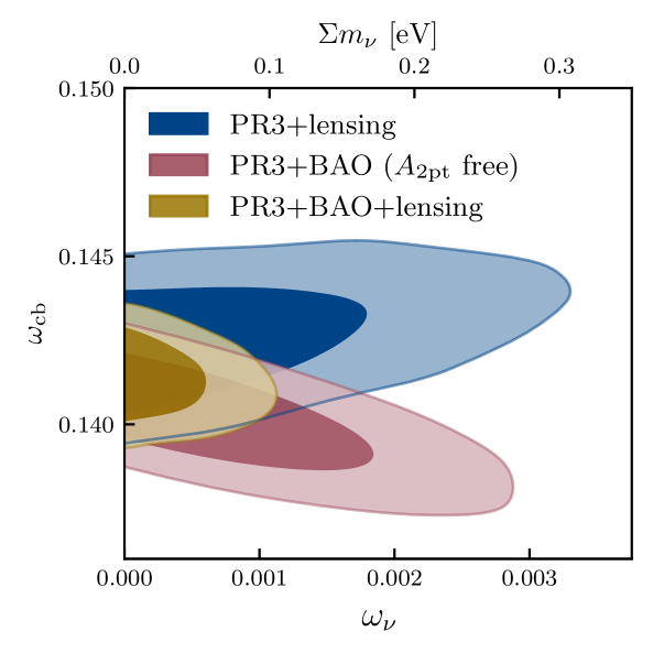
Figure 3: Constraints in the $\omega_{\nu}-\omega_{\rm cb}$ plane reveal the complementary nature of CMB lensing and BAO measurements for determining $\omega_{\nu}$ or, equivalently, $\Sigma m_{\nu}$. BAO data, combined with primary CMB data, are sensitive to the sum $\omega_{\nu}+\omega_{\rm cb}$ while lensing data are sensitive to a combination that is close to the difference $\omega_{\rm cb}-\omega_{\nu}$. Since primary CMB data are sensitive to $\omega_{\rm cb}$ the degeneracies are only approximate and the contours close. To avoid lensing information affecting the BAO result here we marginalized over $A_{\rm 2pt}$.

This is shown in detail in Fig. 3. As discussed above, to get constraints in this plane from BAO data we need to add in primary CMB data. For our purposes here, we want to do so without including any lensing information, so we marginalize over $A_{\rm 2pt}$. We indeed see approximate degeneracies in the two sets of constraints, with the BAO one approximately along a line of constant $\omega_{\rm cb}+\omega_{\nu}$ and the lensing one approximately along a line of constant $\omega_{\rm cb}-0.5\omega_{\nu}$.

This figure explains why BAO data are more effective than CMB lensing data at constraining the neutrino mass, when combined with measurements of the CMB power spectra. The primary CMB (ignoring lensing effects) is hardly sensitive to neutrino masses in the range displayed, so it essentially constrains $\omega_{\rm cb}$ alone. The constraint in the $\omega_{\rm cb}-\omega_{\nu}$ plane would be close to a horizontal band. With lensing effects included, the primary CMB gains sensitivity to this mass range, but the sensitivity is weak and approximately falls along a line of constant $\omega_{\rm cb}-0.2\omega_{\nu}$. BAO data, with their constraint falling along $\omega_{\rm m}+\omega_{\rm cb}$, leads to tighter constraints because this direction is less aligned with constant $\omega_{\rm cb}-0.2\omega_{\nu}$ than is the constraint from adding in lensing reconstruction data, approximately $\omega_{\rm cb}-0.5\omega_{\nu}$. Of course, adding both BAO and CMB lensing reconstruction data leads to greater improvements, since these contours are even less aligned with each other, as shown with the yellow contour in Fig. 3.

It is also evident from this figure that CMB lensing data prefer higher values of $\omega_{\rm cb}$ than do BAO data, in combination with primary CMB data. One implication of this is that, in the $\mbox{$\Lambda$CDM}\ +\mbox{$\Sigma m_{\nu}$}$ model space, the lensing excess and matter deficit signatures are closely related. The low matter density preferred by BAO data when combined with primary CMB data reduces somewhat the expected lensing power, which contributes to the excess lensing problem. Similarly, the lensing reconstruction (and peak-smearing in the CMB power spectra) both prefer higher $\omega_{\rm c}$, and therefore $\omega_{\rm cb}$, which worsens the matter deficit.

We find it interesting that we can use Planck primary CMB data to set expectations for each of these probes, for a continuum of values of $\Sigma m_{\nu}$, and in both cases what is observed is the opposite of expectations assuming $\mbox{$\Sigma m_{\nu}$}>0$.

III Background preference for $\omega_{\rm m}<\omega_{\rm cb}$

In this section we quantify the preference, noticed by Loverde and Weiner [16], of BAO plus CMB data for a total non-relativistic matter density today that is less than the sum of baryonic and cold dark matter density today. We do so by defining a toy model with an effective neutrino mass parameter that can take on negative values, to allow for the possibility that $\omega_{\rm m}<\omega_{\rm cb}$. Such a difference could then be interpreted as a “negative effective neutrino density” $\omega_{\bar{m}_{\nu}}\equiv\omega_{\rm m}-\omega_{\rm cb}$. This is similar in spirit to previous effective “negative neutrino mass” implementations [13, 14, 15], but one which only models the impact of the neutrino on the background evolution. We first discuss our implementation of the model, as well as our method for comparing to data while only modeling the background evolution. We then present the results of this analysis, which show a preference from CMB+BAO data for a matter-density deficit.

III.1 Model

Here we construct a phenomenological model of the background evolution with an effective neutrino mass parameter that is allowed to be negative. We assume two species of massless neutrino, which behave in the standard way, and one neutrino with this effective mass. Additionally, we set $\hbar=k_{B}=c=1$. That being the case, the energy density and pressure of the one massive neutrino species are computed from Fermi-Dirac integrals over neutrino momentum:

$$\rho_{m_{\nu}}(z) =\frac{T_{\nu}(z)^{4}}{\pi^{2}}\int_{0}^{\infty}\frac{x^{2}}{e^{x}+1}\left(x^{2}+\frac{m_{\nu}^{2}}{T_{\nu}(z)^{2}}\right)^{1/2}$$ (6)

$$3p_{m_{\nu}} =\frac{T_{\nu}(z)^{4}}{\pi^{2}}\int_{0}^{\infty}\frac{x^{4}}{e^{x}+1}\left(x^{2}+\frac{m_{\nu}^{2}}{T_{\nu}(z)^{2}}\right)^{-1/2}.$$ (7)

The neutrino temperature follows the usual scaling $T_{\nu}(z)=T_{\nu,0}(1+z)$. For massless particles, $\rho=3p$. We use this fact to define the ‘matter-like’ and ‘radiation-like’ components of the massive neutrino energy density:

$$\omega_{m_{\nu},m} \equiv\left(\rho_{m_{\nu}}(z)-3p_{m_{\nu}}\right)/\rho_{c,100}$$ (8)

$$\omega_{m_{\nu},r} \equiv 3p_{m_{\nu}}/\rho_{c,100}$$ (9)

The denominator in these expressions is the critical density for a universe in which $H_{0}=100\text{ km/s/Mpc}$, $\rho_{c,100}\simeq 1.88\times 10^{-29}\text{ g/cm}^{3}$.

We now extend the model of the energy density to a phenomenological one that allows for the neutrino rest-mass contribution to the energy density ($\omega_{\bar{m}_{\nu}}$) to be negative via:

$$\omega_{\bar{m}_{\nu}}=\omega_{m_{\nu},r}+\text{sgn}(\bar{m}_{\nu})\omega_{m_{\nu},m}$$ (10)

where $\bar{m}_{\nu}$ is what we call the ‘effective neutrino mass parameter’ with $\bar{m}_{\nu}^{2}=m_{\nu}^{2}$. When $\bar{m}_{\nu}\geq 0$, this definition is identical to the energy density for physical neutrinos. However, when $\bar{m}_{\nu}<0$, the contribution to the total neutrino energy density coming from the neutrino rest mass is subtracted rather than added. When referring to the total matter density $\omega_{\rm m}$ in our model, we likewise add or subtract $\omega_{m_{\nu},m}$:

$$\omega_{\rm m}=\omega_{\rm c}+\omega_{\rm b}+\text{sgn}(\bar{m}_{\nu})\omega_{m_{\nu},m}$$ (11)

This allows for $\omega_{\rm m}<\omega_{\rm cb}$ at late times, as desired.

The radiation density can be written in terms of the photon density, which is tightly constrained from the local measurement of the CMB temperature [17]:

$$\omega_{r}(z)=\omega_{\gamma}(z)\left(1+\frac{7}{8}\left(\frac{T_{\nu}}{T_{\gamma}}\right)^{4}N_{\rm ur}\right)$$

where $N_{\rm ur}$ denotes the number of additional ultra-relativistic degrees of freedom, in our case consisting of two massless neutrinos. Finally, we assume spatial flatness, so that the dark energy density is related to the other parameters through:

$$\omega_{\Lambda}=h^{2}-\omega_{\rm c}-\omega_{\rm b}-\omega_{r}-\omega_{\bar{m}_{\nu}}$$

With all of these definitions, the Friedmann equation in our model is given by

$$h^{2}(z)=\omega_{\rm c}(z)+\omega_{\rm b}(z)+\omega_{r}(z)+\omega_{\bar{m}_{\nu}}(z)+\omega_{\Lambda}$$ (12)

We note that there are multiple ways to define an effective neutrino mass parameter at the background level. Our implementation isolates the effect of massive neutrinos on the matter density $\omega_{\rm m}$, and for negative values of $\bar{m}_{\nu}$, that effect is the opposite of the positive mass case. However, there are other ways that massive neutrinos affect the background evolution, beyond contributing to the matter density: namely, in a model with some number of massive neutrinos, the radiation density is reduced relative to the case of massless neutrinos once the neutrino rest mass becomes important. In our model, this reduction of the radiation density is the same for both positive and negative values of $\bar{m}_{\nu}$. Consequently, for fixed $|\bar{m}_{\nu}|$, $\bar{m}_{\nu}<0$ has a greater impact on the expansion history than does $\bar{m}_{\nu}>0$. This is apparent from the asymmetry in the effect on the expansion rate between $\bar{m}_{\nu}=0.1\text{ eV}$ and $\bar{m}_{\nu}=-0.1\text{ eV}$ in Fig. 1. This makes constraints in our model conservative, at least compared to a symmetric implementation one might have chosen instead which also reverses the impact of mass on the radiation density.

Finally, in addition to the Friedmann equation, we also need to compute quantities such as $\theta_{s}^{\star}$ or $D_{A}^{\star}$, which depend on the details of the recombination process. We use the HYREC-2 recombination code [41, 42] for these calculations..

In total, our model is determined by four free parameters, $\{h,\omega_{\rm b},\omega_{\rm c},\bar{m}_{\nu}\}$. Here, $h$ is the dimensionless Hubble parameter $h\equiv H_{0}/\left(100\text{ km/s/Mpc}\right)$, and $\omega_{\rm b}$ and $\omega_{\rm c}$ are the usual baryon and dark matter densities.

III.2 Data

Table 1: Glossary of data sets and background-only likelihoods labels used in this work. The background-only likelihoods are constructed according to the the procedure outlined in Section III.2, using the data listed in the table. The BAO data set we use is the composite data set suggested by Adame et al. [39], with the addition of the low redshift 6dF measurement.

Name	Description
PR3	Planck 2018 Commander low-$\ell$ TT, SimAll low-$\ell$ EE, and Plik (nuisance parameter marginalized) high-$\ell$ TTTEEE likelihoods [43]
PR4	Planck 2018 Commander low-$\ell$ TT, LoLLiPoP low-$\ell$ EE, and HiLLiPoP high-$\ell$ TTTEEE [6] likelihoods using the Planck PR4 NPIPE data [44]
BAO	The 6dF measurement at $z_{\rm eff}=.106$ [45], SDSS DR7 MGS [46] and SDSS DR12 LRG results at $z_{\rm eff}=0.38$ and $0.51$ [36], DESI Y1 results at $z_{\rm eff}>0.6$ [39]. We use the joint eBOSS+DESI Ly$\alpha$ BAO measurement [37, 8] instead of the DESI-only measurement.
lensing	ACT DR6 lensing [7, 12] in combination with Planck PR4 lensing [11].
PR3-B	Background-only likelihood using PR3 data
NoLens-B	Background-only likelihood using PR3 data, after removing lensing information by marginalizing over $A_{\rm 2pt}$
PR4-B	Background-only likelihood using PR4 data
BAO-cb	The BAO likelihoods indicated above, in combination with a joint prior on $\omega_{\rm c}$ and $\omega_{\rm b}$ from one of the CMB likelihoods (the specific one depending on context).

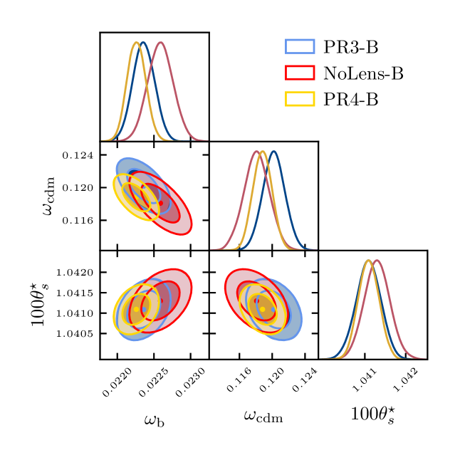
Figure 4: One and two-dimensional marginal posterior distributions for the ’background’ CMB-derived parameters (see text), for the ’Background-only’ (B) likelihoods. The B likelihoods are Gaussian fits to the full likelihoods, whose two-dimensional marginal posterior distributions are shown here as filled contours. The Gaussian fits are sufficiently good approximations that no differences can be seen here. The likelihoods used are described in Table 1. All contour plots are made using the GetDist package [47].

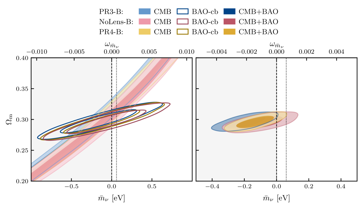
Figure 5: Left panel: Constraints from CMB and BAO data, considered separately, using the three background-only likelihoods. For the CMB constraint, we use the full three parameter background-only likelihood, whereas for the BAO-cb constraints we use BAO likelihoods along with a joint Gaussian prior on $\omega_{\rm b}$ and $\omega_{\rm c}$ with covariance given obtained from the background-only likelihood. The top axis shows the effective neutrino energy density using $\bar{m}_{\nu}/93.14\text{ eV}=\omega_{\bar{m}_{\nu}}$. Right panel: The constraints using the background-only CMB likelihood jointly with BAO data.

The model introduced in the previous section incorporates an effective positive (negative) neutrino mass parameter into the background evolution by adding (subtracting) the contribution towards the total neutrino energy density coming from the neutrino rest mass. With a negative effective neutrino energy density, there is no clear way to define and track neutrino perturbations, and so it is not possible to use full CMB likelihoods to constrain our model. Instead, using constraints obtained from CMB analyses with the full likelihood, we create “background-only” likelihoods which encapsulate the CMB information about the post-recombination background evolution.

As discussed in Section II, of the six $\Lambda$CDM parameters, the physical baryon and dark matter densities, along with the angular scale of the sound horizon, $\vec{\theta}=\left(\omega_{\rm c},\omega_{\rm b},\theta_{s}^{\star}\right)^{\intercal}$, are well determined from the CMB and are sufficient (within $\Lambda$CDM) to determine the post-recombination background evolution. We use the marginal posteriors of these parameters, coming from full CMB analyses, to construct three background-only likelihoods as follows.

Given samples from the posterior distribution under some dataset and model, we construct a parameter covariance matrix $\Sigma\equiv\text{cov}\left(\vec{\theta},\vec{\theta}\right)$. We use this to construct a Gaussian approximation to the marginal posterior in this 3-dimensional subspace. We choose the mean value of these parameters as the “data vector”, so that the background-only likelihood is

$$\ln{\mathcal{L}}=\left(\vec{\theta}-\vec{\theta}_{\rm data}\right)^{\intercal}\Sigma^{-1}\left(\vec{\theta}-\vec{\theta}_{\rm data}\right).$$ (13)

To distinguish these likelihoods from the full likelihoods from which they are constructed, we denote them with a “-B” suffix. The “background-only” nomenclature is meant to convey that these likelihoods encapsulate the CMB constraint on the post-recombination background evolution. This approach to compressing CMB information has been used in the past, e.g. in [40].

The data we use to create these likelihoods is summarized in Table 1. For our baseline CMB data, we use Planck PR3 data, and construct the baseline background-only likelihood from posterior samples assuming $\Lambda$CDM. However, the lensing information in the CMB two point functions plays an important role in setting expectations for $\omega_{\rm cb}$, which is relevant to our analysis. We therefore also create a likelihood from posterior samples using PR3 data, after marginalizing over $A_{\rm 2pt}$. Finally, we create a likelihood from Planck PR4 data, where the $A_{\rm 2pt}$ excess is not as significant. These background-only likelihoods are shown in Fig. 4.

We also define a set of “BAO-cb” likelihoods, capable of constraining $\bar{m}_{\nu}$. Each one is an extension of the BAO likelihood combination listed in Table 1 to include a joint posterior of $\omega_{\rm b}$ and $\omega_{\rm c}$ obtained by marginalizing either PR3-B, NoLens-B, or PR4-B over $\theta_{\rm s}$. With this extension, we can plot BAO constraints (with this CMB prior) directly in the $\Omega_{\rm m}-\bar{m}_{\nu}$ plane after marginalizing over uncertainties in $\omega_{\rm b}$ and $\omega_{\rm c}$. This is similar to the $\Omega_{m}-\omega_{\rm m}r_{\rm d}^{2}$ plane used by Loverde and Weiner [16], but allows us to marginalize over the CMB information instead of assuming fiducial values. Note that we use Equation 5, with $\Sigma m_{\nu}$ replaced by $\bar{m}_{\nu}$, and $r_{\rm s,f}$ replaced with $r_{\rm s}$ to plot in this plane. Since $\omega_{\rm m}r_{\rm s}^{2}$ can be determined from BAO data, and the remaining quantities can be determined from $\omega_{\rm b}$ and $\omega_{\rm c}$, the BAO-bc likelihoods are indeed capable of constraining $\bar{m}_{\nu}$, as desired.

III.3 Results

Table 2: Priors used for the background-only and DDM analyses presented in this work. In the DDM analysis, $\Gamma$ is treated as a derived parameter following the relationship discussed in Section IV. In both analyses, we assume two massless and one massive species of neutrino.

Model	Parameter	Prior
Background only	$h$	$\mathcal{U}[0.4,1]$
	$\omega_{\rm b}$	$\mathcal{U}[0.005,1]$
	$\omega_{\rm c}$	$\mathcal{U}[0.001,0.99]$
	$\bar{m}_{\nu}$	$\mathcal{U}[-1,1]$
DDM	$100\theta_{s}^{\star}$	$\mathcal{U}[0.5,5]$
	$\omega_{\rm b}$	$\mathcal{U}[0.005,1]$
	$\omega_{\rm c}$	$\mathcal{U}[0.001,0.99]$
	$\ln\left(10^{10}A_{s}\right)$	$\mathcal{U}[1.61,3.91]$
	$n_{s}$	$\mathcal{U}[0.8,1.2]$
	$\tau_{\rm reio}$	$\mathcal{U}[0.01,0.8]$
	$\Sigma m_{\nu}$	$\mathcal{U}[0.0,3.0]$
	$\omega_{\rm ddm}^{\rm ini}$	$\mathcal{U}[0.0,0.01]$
	$A_{\rm 2pt}$	$\mathcal{U}[0,10]$

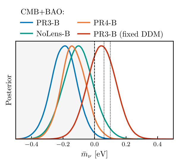
Figure 6: One-dimensional marginal posteriors for the effective neutrino mass parameter $\bar{m}_{\nu}$ given several different background-only CMB + BAO likelihoods. All cases assume $\Lambda$CDM with extension to free $\bar{m}_{\nu}$. The one labeled ‘fixed DDM’ includes a contribution from decaying dark matter with fixed model parameters described in Section IV.

We constrain the four-parameter effective neutrino mass background model in an MCMC analysis with the COBAYA [48] sampler, using the reduced CMB and BAO likelihoods and BAO data just described. We consider chains as converged when the Gelman-Rubin statistic is at $R-1<0.01$. Parameter constraints are reported as 68% confidence intervals.

We begin with a comparison between a result derived with physical neutrino masses and a result in our effective neutrino mass model, in the regime where they can be compared, namely for $\bar{m}_{\nu}\,>\,0$. We run a chain with the PR3-B and BAO likelihoods, with a prior that $\bar{m}_{\nu}\,>\,0$. The resulting constraint on $\bar{m}_{\nu}$ is shown as the blue dashed line in Fig. 6; it is very similar to the corresponding constraint from the full likelihoods with physical neutrino masses, shown as the solid blue line. This agreement supports our expectation that the compression of CMB information to the B likelihoods has not lost any significant information relevant to $\Sigma m_{\nu}$ or $\bar{m}_{\nu}$.

We now move on to cases where $\bar{m}_{\nu}$ can be negative. With the baseline PR3-B likelihood, we find a significant preference for $\omega_{\rm m}<\omega_{\rm cb}$, with

$$\bar{m}_{\nu}=-0.193\pm 0.083\text{ eV}.$$ (14)

This excludes $0.06$ eV, the minimum mass in the NO, at $3\,\sigma$. This likelihood includes the effects of lensing in the two point function, and correspondingly $\omega_{\rm c}$ adjusts towards higher values to fit the features in the Planck data driving the $A_{\rm 2pt}$ anomaly. To assess the impact of this, we can use the NoLens-B likelihood, where lensing information has been removed by marginalizing over $A_{\rm 2pt}$. In that case, we find instead a weaker preference

$$\bar{m}_{\nu}=-0.103\pm 0.096\text{ eV}.$$ (15)

which is $1.7\,\sigma$ away from the NO minimum mass. Finally, with the PR4-B likelihood, the constraint is

$$\bar{m}_{\nu}=-0.132\pm 0.079\text{ eV}.$$ (16)

which is $2.4\,\sigma$ away from the NO minimum mass. These posteriors are shown in Fig. 6.

III.3.1 Discussion

In Fig. 5, we demonstrate how the separate CMB-B and BAO constraints interact to produce this preference for a negative effective neutrino mass at the background level. In the left panel, we show the CMB-B and BAO constraints separately in the $\bar{m}_{\nu}-\Omega_{\rm m}$ plane. As anticipated from the discussion in Section II, when only CMB data are used there is a broad degeneracy in this plane that stems from the degeneracy between $\omega_{\bar{m}_{\nu}}$ and $\omega_{\Lambda}$ that keeps the distance to last scattering fixed. BAO data, when the sound horizon $r_{\rm d}$ is calibrated from the CMB prior on $\omega_{\rm b}$ and $\omega_{\rm c}$, can directly constrain low-redshift distances. Combined with the value of $\omega_{\rm cb}$ obtained from the CMB prior, this results in the unfilled contours in the left-hand panel.

Examining these constraints separately helps to isolate the impact of the shifts in $\omega_{\rm cb}$ when marginalizing over $A_{\rm 2pt}$. The excess lensing-like smoothing that is present in PR3 data is not well fit within $\Lambda$CDM: the fit improves by $\Delta\chi_{\rm eff}^{2}\approx-10$ when $A_{\rm 2pt}$ is freed [1]. $A_{\rm 2pt}$ is not a physical parameter however, and these improved fits have a lower matter density than is preferred by $\Lambda$CDM. These shifts are visible in the reduced likelihoods shown in Fig. 4. We see from the right panel of Fig. 5, and from the decreased tension with the NO minimum mass when $A_{\rm 2pt}$ is freed, that these shifts impact the significance of the $\omega_{\rm m}<\omega_{\rm cb}$ preference.

Shifting $\omega_{\rm cb}$ downwards moves both the CMB and BAO constraints towards higher values of $\bar{m}_{\nu}$ for fixed values of $\Omega_{\rm m}$. This can be understood by considering the constraint on $\omega_{\bar{m}_{\nu}}=\omega_{\rm m}-\omega_{\rm cb}$. When the lensing amplitude is free, and the CMB prefers lower values of $\omega_{\rm cb}$, the difference $\omega_{\rm m}-\omega_{\rm cb}$ required for consistency between CMB and BAO data is lessened, resulting in a milder preference for $\omega_{\rm m}<\omega_{\rm cb}$. With the PR4 likelihoods that we use, the excess peak smearing in the power spectra is reduced, with $A_{\rm 2pt}=1.039\pm 0.052$ ($0.7\,\sigma$ from unity). Here, the inferred $\omega_{\rm cb}$ is higher than it is when using PR3 data and marginalizing over $A_{\rm 2pt}$, as the dark matter density must still adjust (towards higher values) to fit the peak smoothing.

The correlation between $A_{\rm 2pt}$ and $\omega_{\rm cb}$, which arises due to the role $\omega_{\rm cb}$ plays in the lensing of primary CMB power spectra, leads to one interesting conclusion: extensions to $\Lambda$CDM that predict a higher lensing power ($\Lambda$CDM+$A_{2\rm pt}$ being an example, albeit not a physical one) could potentially solve both the lensing excess and the matter deficit.

One can also see in Fig. 5 how adding the $\theta_{s}^{\star}$ constraint significantly tightens the BAO constraint on $\bar{m}_{\nu}$. Note the change in $x$ axis between the left and right panels.

IV Case study: Decaying dark matter

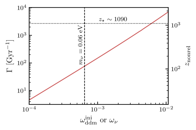
Figure 7: The relationship between decay rate $\Gamma$ and the initial decaying dark matter density parameter $\omega_{\rm ddm}^{\rm ini}$ in our reduced-dimensionality decaying dark matter parameter space (left-hand $y$ axis), and the relationship between a given neutrino energy density today $\omega_{\nu}$ and the redshift of the neutrino’s relativistic to non-relativistic transition (right-hand $y$ axis). In our DDM model, the decay rate is a derived parameter, chosen such that a given $\omega_{\rm ddm}^{\rm ini}$ decays at the non-relativistic transition redshift for $\omega_{\nu}=\omega_{\rm ddm}^{\rm ini}$ assuming one species of massive neutrino. This ensures the DDM is degenerate with neutrino mass in its effect on the background expansion. For reference, the density corresponding to $m_{\nu}=0.06$ eV is marked, as is the redshift (and corresponding decay rate) of last scattering.

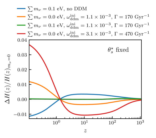
Figure 8: Changes to the expansion rate caused by neutrino mass can be mimicked by decaying dark matter. Here we show several departures from the case of zero neutrino mass and zero decaying dark matter. Information in the legend about the green curve indicates the decaying dark matter parameter values that can be used to compensate for $\Sigma m_{\nu}=0.1$ eV.

In the previous section, we established that at the background level, the combination of CMB and BAO data shows a preference for a deficit in the matter density, $\omega_{\rm m}<\omega_{\rm cb}$, once freedom has been introduced to allow for that possibility. The phenomenological model we used served to quantify the problem, but is, of course, not a solution.

We now consider a model of decaying dark matter (DDM) with dark radiation (DR) decay products, which, similar to the effective negative neutrino mass model of the previous section, can decrease the comoving matter density after recombination. We show that this model is indeed similar to the effective neutrino mass model at the background level. We then place constraints in a model space where the neutrino mass is free to vary, as is the initial amount of decaying dark matter. We consider this model a case study illustrating how the $\omega_{\rm m}{\,}<{\,}\omega_{\rm cb}$ preference could be explained, without solving the excess lensing problem. Alternatively, this case study illustrates the difficulties in explaining both signals with a physical model.

Decaying dark matter (DDM) models have been studied as potential solutions to both the $S_{8}$ and Hubble tensions [e.g., 49, 50, 51, 52, 53, 54, 55]. CMB, BAO, and other large-scale structure data have been used to constrain the amount and lifetime of DDM [e.g. 56, 57, 58, 59, 60, 61], and a general conclusion from these studies is that DDM models cannot resolve the aforementioned tensions without additional modifications to the cosmological model. These conclusions are also supported by frequentist analyses, which do not depend on the choice of priors, and are not susceptible to volume effects [55, 62, 61].

For our case study, we use the DDM model currently implemented in CLASS [63, 64], which allows one to specify the initial density of DDM, $\omega_{\rm ddm}^{\rm ini}$, as well as the decay rate $\Gamma$. The evolution of the DDM density, and the density of its DR decay product, is given by [65, 57, 58]

$$\dot{\rho}_{\rm ddm} =-3\frac{\dot{a}}{a}\rho_{\rm ddm}-\Gamma\rho_{\rm ddm}\ {\rm and}$$

$$\dot{\rho}_{\rm dr} =-4\frac{\dot{a}}{a}\rho_{\rm dr}+\Gamma\rho_{\rm ddm}$$

where the $\dot{\ }$ indicates differentiation with respect to proper time. Decays become significant (and complete), on a timescale set by $t_{\rm ddm}\sim 1/\Gamma$. The parameter $\omega_{\rm ddm}^{\rm ini}$ is used to set the initial conditions, and is the initial comoving density of decaying dark matter. This model is a special case of the one introduced in [62] and further studied in [55].

Despite the attention they have received in relation to the $H_{0}$ and $S_{8}$ tensions, decaying dark matter models are less studied in the context of free $\Sigma m_{\nu}$. It was noted in Aubourg et al. [40] that DDM has a similar, but opposite, effect as massive neutrinos on he background evolution. Poulin et al. [58] explored this degeneracy further, and showed that it is nearly complete in its impact on the background expansion when two conditions are met. The first is that $\omega_{\rm ddm}^{\rm ini}=\omega_{\nu}$, so that the contribution to $\omega_{\rm m}$ from non-relativistic neutrinos is canceled by the decaying dark matter converting to radiation. The second condition is that the DDM decays at close to the same time as the neutrinos become non-relativistic, i.e. $\Gamma\approx 1/t(z_{\rm nr})$, where $z_{\rm nr}$ is given in Equation. 3. Figure 7 shows this relationship, where we have used the PR3 mean parameters to compute the redshift-time relationship, $z(t)$. For a given $(\mbox{$\Sigma m_{\nu}$},z_{\rm nr})$, the corresponding pair $(\omega_{\rm ddm}^{\rm ini},\Gamma)$ under this relationship will nearly completely cancel the effects of the neutrino mass in the background evolution. We show this explicitly in Fig. 8.

Poulin et al. [58] also demonstrated that this degeneracy is broken in CMB power spectra due to the impact that DDM has on gravitational lensing and large scale polarization, even when moving along the approximate background-preserving degeneracy. The polarization effects manifest as features on large scales; since they are not as important as the lensing effects we are about to discuss, we do not consider them further here. Lensing is affected in DDM models because of the conversion of non-relativistic, non-pressure supported matter to massless particles which do not cluster on sub-horizon scales. The result is that gravitational potentials decay, and lensing is suppressed, despite the reduction in expansion rate that, were it achieved without loss of clustering matter, would result in a boost to lensing.

It is not a priori clear to us if these degeneracy breaking effects are significant enough to exclude DDM models as solutions to the matter-density deficit. In this section, we investigate this possibility. Throughout, we enforce the approximate background-preserving relationship between $\omega_{\rm ddm}^{\rm ini}$ and $\Gamma$. We do so for two reasons. First, the DDM model space is known to suffer from volume effects, which we wish to avoid for the purpose of this case study. Treating $\Gamma$ as a derived parameter will reduce the dimensionality of our parameter space, which helps to mitigate these effects. Second, by enforcing this relationship we are considering an “optimistic” scenario in which the background evolution is nearly unchanged from the $\mbox{$\Sigma m_{\nu}$}=0$, $\Lambda$CDM case: if the model is nonetheless disfavored, we find it unlikely that it would become more favored by introducing changes at the background level.

IV.1 Background analysis

Before performing an analysis in the DDM + $\Sigma m_{\nu}$ parameter space we just described, we first check if adding a fixed amount of DDM into the background analysis of Section III.3 can completely remove the preference for $\omega_{\rm m}<\omega_{\rm cb}$. Specifically, we add fixed $\omega_{\rm ddm}(z)$ and $\omega_{\rm dr}(z)$ components to the Friedmann equations with values that follow from $\omega_{\rm ddm}^{\rm ini}=3.1\times 10^{-3}$ and $\Gamma=470\text{ Gyr}^{-1}$. We show the resulting $\Delta H(z)/H(z)_{m_{\nu}=0}$ as the red curve in Fig. 7. We chose these values to result in an expansion history slightly more extreme than that preferred by PR3 data, which in our effective neutrino mass model corresponds to $\bar{m}_{\nu}=-0.193\text{ eV}$. Therefore, by construction, we expect a preference for positive effective neutrino mass, so as to recover the preferred expansion history (i.e. the blue curve in Fig. 1).

We compute $\omega_{\rm ddm}(z)$ and $\omega_{\rm dr}(z)$ using the DDM implementation in CLASS, and add these as fixed templates in all calculations of $H(z)$ in our background-only analysis. The CMB constrains the dark matter density prior to recombination, so when including DDM in the analysis we treat the $\omega_{\rm c}$ constraint in our background-only likelihoods as a constraint on $\omega_{\rm dm}^{\star}$, the comoving dark matter density (including both stable and decaying particles) at last scattering.

Repeating the analysis using PR3-B, we find

$$\bar{m}_{\nu}=0.045\pm 0.090\text{ eV}$$ (17)

This posterior is shown in Fig. 6. This confirms that, at least at the background level, the matter-density deficit could be explained by a decaying dark matter component along with massive neutrinos.

IV.2 Constraints on DDM + $\Sigma m_{\nu}$

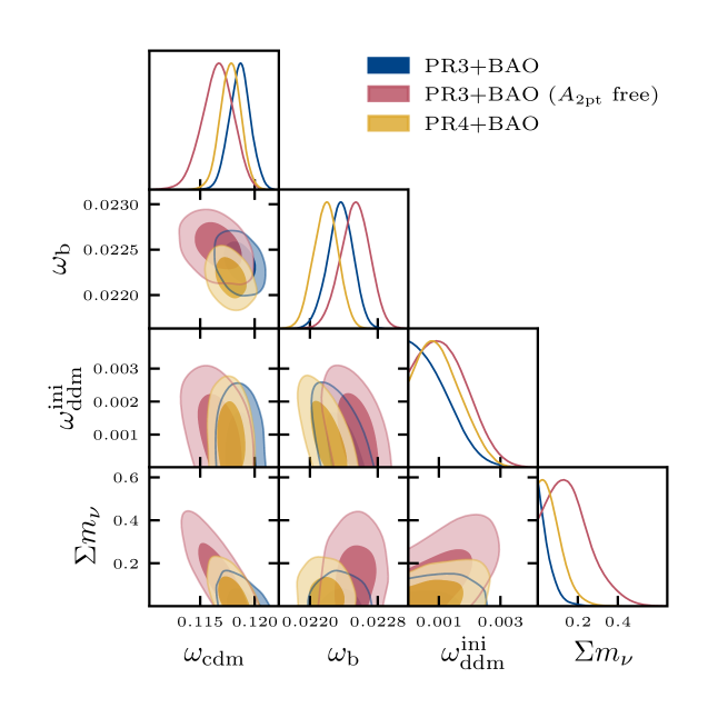
Figure 9: Constraints on density-related parameters in the $\Lambda$CDM + $\Sigma m_{\nu}$ + decaying dark matter parameter space. These constraints are from the full CMB TT/TE/EE Planck likelihoods as described in Tab. 1. Note that lensing information allows for tight constraints on both the decaying dark matter and neutrino mass despite the geometric near-degeneracy shown in Fig. 8.

We now perform a full analysis of the DDM + $\Sigma m_{\nu}$ model using the CMB and BAO data listed in Table 1. We sample over eight parameters, $\vec{\theta}=\{\omega_{\rm c},\omega_{\rm b},100\theta_{s}^{\star},\tau_{\rm reio},n_{s},\ln{\left(10^{10}A_{s}\right)},\omega_{\rm ddm}^{\rm ini},\mbox{$\Sigma m_{\nu}$}\}$, with $\Gamma$ treated as a derived parameter. Our priors are listed in Table 2. For CMB data, we separately consider both PR3 and PR4 data, combining with BAO data in each case. For PR3 data, we also consider the case where $A_{\rm 2pt}$ is free, to assess the impact that the lensing-induced peak smearing has on the constraints. We run each chain until the Gelman-Rubin statistic is at $R-1<0.04$.

The constraints on the various physical matter densities are shown in Fig. 9. We see that even with the possibility of some amount of DDM, the PR3 data still tightly constrain $\Sigma m_{\nu}$. When $A_{\rm 2pt}$ is allowed to freely vary, however, we see a shift in posteriors toward higher values of $\omega_{\rm ddm}^{\rm ini}$ and $\Sigma m_{\nu}$. This indicates that it is the excess peak smearing present in the PR3 data that leads to the still-tight constraints on $\Sigma m_{\nu}$: any amount of DDM, or any non-zero $\Sigma m_{\nu}$, will suppress lensing power, whereas the PR3 data show a preference for enhanced lensing power. This is consistent with the conclusions of McCarthy and Hill [55], who showed that for general DDM models, the fit to CMB power spectra predominantly degrades at intermediate multipoles where lensing effects are important. Freeing $A_{\rm 2pt}$ removes this constraint, and opens the expected degeneracy between $\omega_{\rm ddm}^{\rm ini}$ and $\Sigma m_{\nu}$. In the PR4 likelihoods that we use, the amount of peak smearing is consistent with $\Lambda$CDM [6], so we might expect the $\omega_{\rm ddm}^{\rm ini}$-$\Sigma m_{\nu}$ degeneracy to more clearly manifest itself. Indeed, we see that switching to the PR4 data leads to a preference for non-zero DDM, and a posterior for $\Sigma m_{\nu}$ that peaks at positive values (although still below 0.06 eV).

V Brief Discussion of Potential Solutions

We now turn to a brief discussion of possible solutions. This discussion serves to further highlight the complementary nature of BAO and CMB lensing for constraining $\Sigma m_{\nu}$: there are model extensions that can solve the matter-density deficit but do not solve the excess lensing (as we have seen with DDM) and vice versa.

We presented one extension, the DDM model, aimed at solving these problems, which we used as a case study. In this extension a fraction of the CDM is unstable and decays to dark radiation. At the background level, the DDM has nearly exactly the opposite impact as $\Sigma m_{\nu}$. As a result, we found that with this model one could eliminate the matter-density deficit relative to minimal NO expectations. In this model, for any value of $\Sigma m_{\nu}$, the expansion rate is lower during the matter-dominated era than is the case for the corresponding $\Lambda$CDM + $\Sigma m_{\nu}$ model. This reduced expansion rate (which on its own would boost clustering) is done by converting clustering matter to radiation, so the lensing power is actually reduced, somewhat exacerbating the excess CMB lensing discrepancy rather than reducing it.

Conversely, a potential solution proposed in Craig et al. [13] for the lensing power excess would probably not eliminate the matter deficit without significant additional model-building requirements. This solution involves the generation of primordial perturbations with a trispectrum that mimics the effects on the CMB from gravitational lensing. In this scenario CMB lensing reconstructions, which assume primordial Gaussianity and are dependent on the trispectrum, would be biased. With the right pattern of non-Gaussianity, that bias would show up as the observed excess of reconstructed CMB lensing power.

Whether such a scenario could also address the matter deficit problem remains to be seen. If the new physics that alters the primordial four-point function also alters the primordial two-point function, then it could in principle change the inference of $\omega_{\rm cb}$ from CMB data in a way that resolves the matter deficit. However, if there is no appreciable change to the primordial two-point functions, and CMB lensing power is unchanged, then the inference of $\omega_{\rm cb}$ from the primary CMB data will remain unchanged and the matter deficit discrepancy will remain.

We also mentioned previously that extensions to $\Lambda$CDM that predict a higher lensing power, such as the phenomenological $\Lambda$CDM+$A_{2\rm pt}$ model, could potentially solve both the excess lensing problem and the matter-density deficit problem. How such a model addresses excess lensing power is obvious. The potential for resolving the matter-density deficit discrepancy follows from the dependence of the inference of $\omega_{\rm cb}$ from primary CMB data. With a boosted lensing power spectrum, the $\omega_{\rm cb}$ inference drops, reducing the significance of the matter-density deficit, although not outright restoring the preference for $\omega_{\rm m}\,>\,\omega_{\rm cb}$.

Finding a physical model that can boost the lensing power above the $\Lambda$CDM result is challenging because in the $\Lambda$CDM model the universe is dominated, for a large majority of the post-recombination doublings of the scale factor, by cold dark matter, which is already at the limit of zero pressure support and (practically) zero free-streaming length. Positive mean curvature ($\Omega_{\rm K}<0$) to reduce the expansion rate would help, but the amount of tolerable curvature is tightly constrained by the combination of $\theta_{s}^{\star}$ and other geometrical probes sensitive to the low-redshift universe. Craig et al. [13] discuss the possibility of boosting growth via an attractive long-range dark matter self-interaction. As they point out, any implementation of this idea in a model will need to evade equivalence-principle limits. Further, the consequences of any cosmological background of the force mediators would need to be understood as well.

Finally, given the implications for the post-recombination expansion history, it is worth mentioning the impact of evolving dark energy, and whether it can solve either or both apparent discrepancies. The DESI Collaboration finds a preference for evolving dark energy, the significance of which increases when other probes of late-time geometry (in this case, uncalibrated supernovae [66, 67, 68]) are included in the analysis [8, 69, 70]. Evolving dark energy models are able to fit the feature in BAO data that, in $\Lambda$CDM  leads to a high cosmological constant — the same feature driving the matter-density deficit highlighted here. Elbers et al. [15] have shown that evolving dark energy models, in conjunction with an effective neutrino mass parameter that admits negative values, prefer positive values for the neutrino mass parameter and non-constant dark energy.

While Elbers et al. [15] showed that evolving dark energy models are able to fit the oscillatory features in the Planck data that contribute to the lensing excess, this is consistent with our expectations given the analysis we have presented in this paper. Exactly because evolving dark energy can allow for a higher matter density, the impact of BAO data on lensing expectations in these model spaces is modified (relative to what happens with $\Lambda$CDM + $\Sigma m_{\nu}$) to allow for higher lensing power, reducing the CMB lensing excess somewhat. That this is only a partial reduction in lensing excess makes sense since even absent BAO data there is an excess of lensing at just less than $2\,\sigma$, as seen in Fig. 20 of [4]. Finally, we should mention that in extended parameter spaces, including evolving dark energy and a free neutrino mass (in addition to other extension parameters), Roy Choudhury and Okumura [71] have found indications of positive neutrino mass and $A_{\rm 2pt}$ consistent with unity — but no preference for evolving dark energy, and with increased uncertainties due to the additional degeneracies.

VI Conclusions

We have two different suggestions of a problem in the $\Lambda$CDM  + $\Sigma m_{\nu}$ model space, given BAO and CMB data, which we have referred to as a lensing power excess and a matter-density deficit. These are not statistically overwhelming discrepancies. Craig et al. [13] quantify the first as a $2.4\,\sigma$ discrepancy, which with the addition of the SPT-3G polarization-only CMB lensing power becomes a $2.7\,\sigma$ discrepancy [4]. Here we have quantified the matter-density deficit (relative to expectations under minimal NO) as a $3\,\sigma$ discrepancy.

The focus of this paper is a description of the problem. We quantified the matter-density deficit and provided a narrative aimed at analytic understanding of the origin of cosmological constraints on $\Sigma m_{\nu}$ from current CMB and BAO data.

We first summarized an analysis by Loverde and Weiner [16]. In brief, BAO data are sensitive to the combination $\omega_{\rm m}r_{\rm d}^{2}$. Since CMB data, in the $\Lambda$CDM + $\Sigma m_{\nu}$ model, can be used to determine $r_{\rm d}$, the combination can be used to infer $\omega_{\rm m}$. The precision of the $\omega_{\rm m}$ inference is then greatly enhanced by including the very tight constraint on $\theta_{s}^{\star}$ as inferred from CMB data. This is because to stay at fixed $\theta_{s}^{\star}$ a $\delta\omega_{\nu}$ must be compensated by a 13 times larger change in the cosmological constant energy density. Finally, since CMB data can determine $\omega_{\rm b}$ and $\omega_{\rm c}$, one can compare with $\omega_{\rm m}=\omega_{\nu}+\omega_{\rm b}+\omega_{\rm c}$ to determine $\omega_{\nu}=\mbox{$\Sigma m_{\nu}$}/93.14$ eV.

We found that current CMB lensing data are sensitive to a linear combination that is approximately $\omega_{\rm cb}-0.5\omega_{\nu}$. We expect that inclusion of more lensing reconstruction data with more weight towards higher $L$ will bring this closer to $\omega_{\rm cb}-\omega_{\nu}$. With current data, though, BAO lead to a slightly tighter constraint on their $\omega_{\rm cb},\omega_{\nu}$ linear combination ($\omega_{\rm cb}+\omega_{\nu}$) than is the case for the CMB lensing combination. More importantly, the BAO degeneracy direction in this plane is less parallel to the primary CMB constraint (sensitive to $\simeq\omega_{\rm cb}-0.2\omega_{\nu}$), than is the case for the CMB lensing linear combination. For these reasons, we saw that when adding either BAO data or CMB lensing reconstruction data to lensed primary CMB data, it is the BAO addition that delivers tighter $\Sigma m_{\nu}$ constraints.

We have also quantified the second of the aforementioned problems in the $\mbox{$\Lambda$CDM}+\mbox{$\Sigma m_{\nu}$}$ model space, namely the matter-density deficit. Using a phenomenological model, and comparing to the density expected in $\Lambda$CDM with $\mbox{$\Sigma m_{\nu}$}=0.06\,{\rm eV}$, we find a $3.0\,\sigma$ preference for a deficit, when using the Planck PR3 likelihood. This preference is reduced to $2.4\,\sigma$ when using a Planck PR4 likelihood, and further reduced to $1.7\,\sigma$ when marginalizing over $A_{\rm 2pt}$ with the PR3 likelihood. These changes in significance are a result of shifts in the inferred $\omega_{\rm cb}$ to lower values, reducing the difference $\omega_{\rm m}-\omega_{\rm cb}$.

We discussed potential solutions to the excess lensing and matter density deficit, and how the complementary nature of the CMB lensing and BAO probes can be used to discriminate among them. We studied one of these potential solutions in particular, a model of decaying dark matter, along with free $\Sigma m_{\nu}$, and found that while such a model could eliminate the matter deficit, it increases the lensing excess.

As measurements continue to improve, we hope that the framework developed here will be useful in understanding how different cosmological probes contribute to constraints on the neutrino mass.

References

- Aghanim et al. [2020a] N. Aghanim et al. (Planck), Planck 2018 results. VI. Cosmological parameters, Astron. Astrophys. 641, A6 (2020a), [Erratum: Astron.Astrophys. 652, C4 (2021)], arXiv:1807.06209 [astro-ph.CO] .
- Balkenhol et al. [2023] L. Balkenhol et al. (SPT-3G), Measurement of the CMB temperature power spectrum and constraints on cosmology from the SPT-3G 2018 TT, TE, and EE dataset, Phys. Rev. D 108, 023510 (2023), arXiv:2212.05642 [astro-ph.CO] .
- Aiola et al. [2020] S. Aiola et al. (ACT), The Atacama Cosmology Telescope: DR4 Maps and Cosmological Parameters, JCAP 12, 047, arXiv:2007.07288 [astro-ph.CO] .
- Ge et al. [2024] F. Ge et al. (SPT-3G), Cosmology From CMB Lensing and Delensed EE Power Spectra Using 2019-2020 SPT-3G Polarization Data, (2024), arXiv:2411.06000 [astro-ph.CO] .
- Workman et al. [2022] R. L. Workman et al. (Particle Data Group), Review of Particle Physics, PTEP 2022, 083C01 (2022).
- Tristram et al. [2024] M. Tristram et al., Cosmological parameters derived from the final Planck data release (PR4), Astron. Astrophys. 682, A37 (2024), arXiv:2309.10034 [astro-ph.CO] .
- Madhavacheril et al. [2024] M. S. Madhavacheril et al. (ACT), The Atacama Cosmology Telescope: DR6 Gravitational Lensing Map and Cosmological Parameters, Astrophys. J. 962, 113 (2024), arXiv:2304.05203 [astro-ph.CO] .
- Adame et al. [2024a] A. G. Adame et al. (DESI), DESI 2024 VI: Cosmological Constraints from the Measurements of Baryon Acoustic Oscillations, (2024a), arXiv:2404.03002 [astro-ph.CO] .
- Prabhu et al. [2024] K. Prabhu et al. (SPT-3G), Testing the CDM Cosmological Model with Forthcoming Measurements of the Cosmic Microwave Background with SPT-3G, Astrophys. J. 973, 4 (2024), arXiv:2403.17925 [astro-ph.CO] .
- Green and Meyers [2021] D. Green and J. Meyers, Cosmological Implications of a Neutrino Mass Detection, (2021), arXiv:2111.01096 [astro-ph.CO] .
- Carron et al. [2022] J. Carron, M. Mirmelstein, and A. Lewis, CMB lensing from Planck PR4 maps, Journal of Cosmology and Astroparticle Physics 2022 (09), 039, arXiv:2206.07773 [astro-ph].
- Qu et al. [2024] F. J. Qu et al. (ACT), The Atacama Cosmology Telescope: A Measurement of the DR6 CMB Lensing Power Spectrum and Its Implications for Structure Growth, Astrophys. J. 962, 112 (2024), arXiv:2304.05202 [astro-ph.CO] .
- Craig et al. [2024] N. Craig, D. Green, J. Meyers, and S. Rajendran, No s is Good News, (2024), arXiv:2405.00836 [astro-ph.CO] .
- Green and Meyers [2024] D. Green and J. Meyers, The Cosmological Preference for Negative Neutrino Mass, (2024), arXiv:2407.07878 [astro-ph.CO] .
- Elbers et al. [2024] W. Elbers, C. S. Frenk, A. Jenkins, B. Li, and S. Pascoli, Negative neutrino masses as a mirage of dark energy, (2024), arXiv:2407.10965 [astro-ph.CO] .
- Loverde and Weiner [2024] M. Loverde and Z. J. Weiner, Massive neutrinos and cosmic composition, (2024), arXiv:2410.00090 [astro-ph.CO] .
- Fixsen et al. [1996] D. J. Fixsen, E. S. Cheng, J. M. Gales, J. C. Mather, R. A. Shafer, and E. L. Wright, The Cosmic Microwave Background spectrum from the full COBE FIRAS data set, Astrophys. J. 473, 576 (1996), arXiv:astro-ph/9605054 .
- Aghanim et al. [2017] N. Aghanim et al. (Planck), Planck intermediate results. LI. Features in the cosmic microwave background temperature power spectrum and shifts in cosmological parameters, Astron. Astrophys. 607, A95 (2017), arXiv:1608.02487 [astro-ph.CO] .
- Knox and Millea [2020] L. Knox and M. Millea, Hubble constant hunter’s guide, Phys. Rev. D 101, 043533 (2020), arXiv:1908.03663 [astro-ph.CO] .
- de Salas et al. [2021] P. F. de Salas, D. V. Forero, S. Gariazzo, P. Martínez-Miravé, O. Mena, C. A. Ternes, M. Tórtola, and J. W. F. Valle, 2020 global reassessment of the neutrino oscillation picture, JHEP 02, 071, arXiv:2006.11237 [hep-ph] .
- Esteban et al. [2020] I. Esteban, M. C. Gonzalez-Garcia, M. Maltoni, T. Schwetz, and A. Zhou, The fate of hints: updated global analysis of three-flavor neutrino oscillations, JHEP 09, 178, arXiv:2007.14792 [hep-ph] .
- Archidiacono et al. [2020] M. Archidiacono, S. Hannestad, and J. Lesgourgues, What will it take to measure individual neutrino mass states using cosmology?, JCAP 09, 021, arXiv:2003.03354 [astro-ph.CO] .
- Pan and Knox [2015] Z. Pan and L. Knox, Constraints on neutrino mass from Cosmic Microwave Background and Large Scale Structure, Mon. Not. Roy. Astron. Soc. 454, 3200 (2015), arXiv:1506.07493 [astro-ph.CO] .
- Hou et al. [2014] Z. Hou et al., Constraints on Cosmology from the Cosmic Microwave Background Power Spectrum of the 2500 deg2 SPT-SZ Survey, Astrophys. J. 782, 74 (2014), arXiv:1212.6267 [astro-ph.CO] .
- Lesgourgues et al. [2013] J. Lesgourgues, G. Mangano, G. Miele, and S. Pastor, Neutrino Cosmology (Cambridge University Press, 2013).
- Zaldarriaga and Seljak [1998] M. Zaldarriaga and U. Seljak, Gravitational lensing effect on cosmic microwave background polarization, Phys. Rev. D 58, 023003 (1998), arXiv:astro-ph/9803150 .
- Hirata and Seljak [2003] C. M. Hirata and U. Seljak, Analyzing weak lensing of the cosmic microwave background using the likelihood function, Phys. Rev. D 67, 043001 (2003), arXiv:astro-ph/0209489 .
- Okamoto and Hu [2003] T. Okamoto and W. Hu, CMB lensing reconstruction on the full sky, Phys. Rev. D 67, 083002 (2003), arXiv:astro-ph/0301031 .
- Millea et al. [2020] M. Millea, E. Anderes, and B. D. Wandelt, Sampling-based inference of the primordial CMB and gravitational lensing, Phys. Rev. D 102, 123542 (2020), arXiv:2002.00965 [astro-ph.CO] .
- Lewis and Challinor [2006] A. Lewis and A. Challinor, Weak gravitational lensing of the CMB, Phys. Rept. 429, 1 (2006), arXiv:astro-ph/0601594 .
- Kaplinghat et al. [2003] M. Kaplinghat, L. Knox, and Y.-S. Song, Determining neutrino mass from the CMB alone, Phys. Rev. Lett. 91, 241301 (2003), arXiv:astro-ph/0303344 .
- Allali and Notari [2024] I. J. Allali and A. Notari, Neutrino mass bounds from DESI 2024 are relaxed by Planck PR4 and cosmological supernovae, JCAP 12, 020, arXiv:2406.14554 [astro-ph.CO] .
- Naredo-Tuero et al. [2024] D. Naredo-Tuero, M. Escudero, E. Fernández-Martínez, X. Marcano, and V. Poulin, Critical look at the cosmological neutrino mass bound, Phys. Rev. D 110, 123537 (2024), arXiv:2407.13831 [astro-ph.CO] .
- Di Valentino and Melchiorri [2022] E. Di Valentino and A. Melchiorri, Neutrino Mass Bounds in the Era of Tension Cosmology, Astrophys. J. Lett. 931, L18 (2022), arXiv:2112.02993 [astro-ph.CO] .
- Pan et al. [2014] Z. Pan, L. Knox, and M. White, Dependence of the Cosmic Microwave Background Lensing Power Spectrum on the Matter Density, Mon. Not. Roy. Astron. Soc. 445, 2941 (2014), arXiv:1406.5459 [astro-ph.CO] .
- Alam et al. [2017] S. Alam et al. (BOSS), The clustering of galaxies in the completed SDSS-III Baryon Oscillation Spectroscopic Survey: cosmological analysis of the DR12 galaxy sample, Mon. Not. Roy. Astron. Soc. 470, 2617 (2017), arXiv:1607.03155 [astro-ph.CO] .
- Alam et al. [2021] S. Alam et al. (eBOSS), Completed SDSS-IV extended Baryon Oscillation Spectroscopic Survey: Cosmological implications from two decades of spectroscopic surveys at the Apache Point Observatory, Phys. Rev. D 103, 083533 (2021), arXiv:2007.08991 [astro-ph.CO] .
- Adame et al. [2024b] A. G. Adame et al. (DESI), DESI 2024 III: Baryon Acoustic Oscillations from Galaxies and Quasars, (2024b), arXiv:2404.03000 [astro-ph.CO] .
- Adame et al. [2025] A. G. Adame et al. (DESI), DESI 2024 IV: Baryon Acoustic Oscillations from the Lyman alpha forest, JCAP 01, 124, arXiv:2404.03001 [astro-ph.CO] .
- Aubourg et al. [2015] E. Aubourg et al. (BOSS), Cosmological implications of baryon acoustic oscillation measurements, Phys. Rev. D 92, 123516 (2015), arXiv:1411.1074 [astro-ph.CO] .
- Ali-Haïmoud and Hirata [2011] Y. Ali-Haïmoud and C. M. Hirata, Hyrec: A fast and highly accurate primordial hydrogen and helium recombination code, Phys. Rev. D 83, 043513 (2011).
- Lee and Ali-Haïmoud [2020] N. Lee and Y. Ali-Haïmoud, hyrec-2: A highly accurate sub-millisecond recombination code, Phys. Rev. D 102, 083517 (2020).
- Aghanim et al. [2020b] N. Aghanim et al. (Planck), Planck 2018 results. V. CMB power spectra and likelihoods, Astron. Astrophys. 641, A5 (2020b), arXiv:1907.12875 [astro-ph.CO] .
- Akrami et al. [2020] Y. Akrami et al. (Planck), intermediate results. LVII. Joint Planck LFI and HFI data processing, Astron. Astrophys. 643, A42 (2020), arXiv:2007.04997 [astro-ph.CO] .
- Beutler et al. [2011] F. Beutler, C. Blake, M. Colless, D. H. Jones, L. Staveley-Smith, L. Campbell, Q. Parker, W. Saunders, and F. Watson, The 6dF Galaxy Survey: baryon acoustic oscillations and the local Hubble constant, Mon. Not. Roy. Astron. Soc. 416, 3017 (2011), arXiv:1106.3366 [astro-ph.CO] .
- Ross et al. [2015] A. J. Ross, L. Samushia, C. Howlett, W. J. Percival, A. Burden, and M. Manera, The clustering of the SDSS DR7 main Galaxy sample – I. A 4 per cent distance measure at , Mon. Not. Roy. Astron. Soc. 449, 835 (2015), arXiv:1409.3242 [astro-ph.CO] .
- Lewis [2019] A. Lewis, GetDist: a Python package for analysing Monte Carlo samples, (2019), arXiv:1910.13970 [astro-ph.IM] .
- Torrado and Lewis [2021] J. Torrado and A. Lewis, Cobaya: Code for Bayesian Analysis of hierarchical physical models, JCAP 05, 057, arXiv:2005.05290 [astro-ph.IM] .
- Enqvist et al. [2015] K. Enqvist, S. Nadathur, T. Sekiguchi, and T. Takahashi, Decaying dark matter and the tension in , JCAP 09, 067, arXiv:1505.05511 [astro-ph.CO] .
- Davari and Khosravi [2022] Z. Davari and N. Khosravi, Can decaying dark matter scenarios alleviate both H0 and 8 tensions?, Mon. Not. Roy. Astron. Soc. 516, 4373 (2022), arXiv:2203.09439 [astro-ph.CO] .
- Anchordoqui et al. [2022] L. A. Anchordoqui, V. Barger, D. Marfatia, and J. F. Soriano, Decay of multiple dark matter particles to dark radiation in different epochs does not alleviate the hubble tension, Phys. Rev. D 105, 103512 (2022).
- Haridasu and Viel [2020] B. S. Haridasu and M. Viel, Late-time decaying dark matter: constraints and implications for the -tension, Mon. Not. Roy. Astron. Soc. 497, 1757 (2020), arXiv:2004.07709 [astro-ph.CO] .
- Pandey et al. [2020] K. L. Pandey, T. Karwal, and S. Das, Alleviating the and anomalies with a decaying dark matter model, JCAP 07, 026, arXiv:1902.10636 [astro-ph.CO] .
- Chudaykin et al. [2018] A. Chudaykin, D. Gorbunov, and I. Tkachev, Dark matter component decaying after recombination: Sensitivity to baryon acoustic oscillation and redshift space distortion probes, Phys. Rev. D 97, 083508 (2018), arXiv:1711.06738 [astro-ph.CO] .
- McCarthy and Hill [2023] F. McCarthy and J. C. Hill, Converting dark matter to dark radiation does not solve cosmological tensions, Phys. Rev. D 108, 063501 (2023), arXiv:2210.14339 [astro-ph.CO] .
- Ichiki et al. [2004] K. Ichiki, M. Oguri, and K. Takahashi, WMAP constraints on decaying cold dark matter, Phys. Rev. Lett. 93, 071302 (2004), arXiv:astro-ph/0403164 .
- Audren et al. [2014] B. Audren, J. Lesgourgues, G. Mangano, P. D. Serpico, and T. Tram, Strongest model-independent bound on the lifetime of Dark Matter, JCAP 12, 028, arXiv:1407.2418 [astro-ph.CO] .
- Poulin et al. [2016] V. Poulin, P. D. Serpico, and J. Lesgourgues, A fresh look at linear cosmological constraints on a decaying dark matter component, JCAP 08, 036, arXiv:1606.02073 [astro-ph.CO] .
- Xiao et al. [2020] L. Xiao, L. Zhang, R. An, C. Feng, and B. Wang, Fractional Dark Matter decay: cosmological imprints and observational constraints, JCAP 01, 045, arXiv:1908.02668 [astro-ph.CO] .
- Nygaard et al. [2021] A. Nygaard, T. Tram, and S. Hannestad, Updated constraints on decaying cold dark matter, JCAP 05, 017, arXiv:2011.01632 [astro-ph.CO] .
- Holm et al. [2023] E. B. Holm, A. Nygaard, J. Dakin, S. Hannestad, and T. Tram, PROSPECT: A profile likelihood code for frequentist cosmological parameter inference, (2023), arXiv:2312.02972 [astro-ph.CO] .
- Bringmann et al. [2018] T. Bringmann, F. Kahlhoefer, K. Schmidt-Hoberg, and P. Walia, Converting nonrelativistic dark matter to radiation, Phys. Rev. D 98, 023543 (2018), arXiv:1803.03644 [astro-ph.CO] .
- Lesgourgues [2011] J. Lesgourgues, The Cosmic Linear Anisotropy Solving System (CLASS) I: Overview, arXiv e-prints , arXiv:1104.2932 (2011), arXiv:1104.2932 [astro-ph.IM] .
- Blas et al. [2011] D. Blas, J. Lesgourgues, and T. Tram, The Cosmic Linear Anisotropy Solving System (CLASS). Part II: Approximation schemes, JCAP 2011, 034 (2011), arXiv:1104.2933 [astro-ph.CO] .
- Kang et al. [1993] H.-S. Kang, M. Kawasaki, and G. Steigman, Cosmological evolution of generic early decaying particles and their daughters, Nucl. Phys. B 402, 323 (1993).
- Brout et al. [2022] D. Brout et al., The Pantheon+ Analysis: Cosmological Constraints, Astrophys. J. 938, 110 (2022), arXiv:2202.04077 [astro-ph.CO] .
- Rubin et al. [2023] D. Rubin et al., Union Through UNITY: Cosmology with 2,000 SNe Using a Unified Bayesian Framework, (2023), arXiv:2311.12098 [astro-ph.CO] .
- Abbott et al. [2024] T. M. C. Abbott et al. (DES), The Dark Energy Survey: Cosmology Results with 1500 New High-redshift Type Ia Supernovae Using the Full 5 yr Data Set, Astrophys. J. Lett. 973, L14 (2024), arXiv:2401.02929 [astro-ph.CO] .
- Lodha et al. [2025] K. Lodha et al. (DESI), DESI 2024: Constraints on physics-focused aspects of dark energy using DESI DR1 BAO data, Phys. Rev. D 111, 023532 (2025), arXiv:2405.13588 [astro-ph.CO] .
- Calderon et al. [2024] R. Calderon et al. (DESI), DESI 2024: reconstructing dark energy using crossing statistics with DESI DR1 BAO data, JCAP 10, 048, arXiv:2405.04216 [astro-ph.CO] .
- Roy Choudhury and Okumura [2024] S. Roy Choudhury and T. Okumura, Updated Cosmological Constraints in Extended Parameter Space with Planck PR4, DESI Baryon Acoustic Oscillations, and Supernovae: Dynamical Dark Energy, Neutrino Masses, Lensing Anomaly, and the Hubble Tension, Astrophys. J. Lett. 976, L11 (2024), arXiv:2409.13022 [astro-ph.CO] .