Tomographic electron flow in confined geometries: Beyond the dual-relaxation time approximation

Abstract

Hydrodynamic-like electron flows are typically modeled using the Stokes-Ohm equation or a kinetic description that is based on a dual-relaxation time approximation. Such models assume a short intrinsic mean free path $\ell_{e}$ due to momentum-conserving electronic scattering and a large extrinsic mean free path $\ell_{\text{MR}}$ due to momentum-relaxing impurity scattering. This assumption, however, is overly simplistic and falls short at low temperatures, where it is known from exact diagonalization studies of the electronic collision integral that another large electronic mean free path $\ell_{o}$ emerges, which describes long-lived odd electron modes—this is sometimes known as the tomographic effect. Here, using a matched asymptotic expansion of the Fermi liquid kinetic equation that includes different electron relaxation times, we derive a general asymptotic theory for tomographic flows in arbitrary smooth boundary geometries. Our key results are a set of governing equations for the electron density and electron current, their slip boundary conditions and boundary layer corrections near diffuse edges. We find that the tomographic effect strongly modifies previous hydrodynamic theories for electron flows: In particular, we find that (i) an equilibrium is established in the bulk, where the flow is governed by Stokes-Ohm like equations with significant finite-wavelength corrections, (ii) the velocity slip conditions for these equations are strongly modified from the widely-used hydrodynamic slip-length condition (iii) a large kinetic boundary layer arises near diffuse boundaries of width $\sim\sqrt{\ell_{e}\ell_{o}}$, and (iv) all these effects are strongly suppressed by an external magnetic field. We illustrate our findings for electron flow in a channel. The equations derived here represent the fundamental governing equations for tomographic electron flow in arbitrary smooth geometries.

I Introduction

In the conventional description of a conductor (the so-called Drude or Ohmic picture of transport), the resistance and other electronic material properties are set by an extrinsic momentum-relaxing mean free path $\ell_{\text{MR}}$, which describes the effect of collisions with impurities or phonons. More recently, however, a fundamentally distinct mode of transport has been observed in high-mobility electronic devices that is marked by a hydrodynamic-like flow of charge carriers [1, 2]. Here, frequent momentum-conserving electron-electron collisions set the shortest mean free path $\ell_{\text{e}}$ and are assumed to establish a local thermodynamic equilibrium with a slow spatial transport of density and currents [3]. This leads to collective hydrodynamic flow patterns that have now been experimentally resolved, such as current vortices [4] or Poiseuille flow through a channel [5, 6, 7, 8]. Such hydrodynamic flow depends sensitively on the device geometry.

The state-of-the-art analysis of hydrodynamic electron flows is based on the so-called Stokes-Ohm equation [1, 2], which combines the linearized hydrodynamic equations of laminar flow (the Stokes equation) with a direct momentum-relaxing term that accounts for residual impurity scattering. Electron interactions enter in this equation through a term that describes the diffusion of the velocity, with a diffusion constant set by the electron viscosity $\eta=v_{F}\ell_{e}/4$ (where $v_{F}$ is the Fermi velocity). This term defines a single characteristic electronic mean free path $\ell_{e}$ (i.e., a single electronic relaxation time scale $\tau_{e}=\ell_{e}/v_{F}$) as a microscopic parameter. A solution of the Stokes-Ohm equation in finite device geometries with appropriate boundary condition [9, 10] then provides information on the shear viscosity. The corresponding microscopic kinetic picture, from which the Stokes-Ohm equation is derived in a hydrodynamic limit, is based on the so-called dual relaxation time approximation, originally introduced in this context by De Jong and Molenkamp [11]. Fundamentally, both frameworks are semiclassical descriptions that treat the flow of thermally excited electron quasiparticles through a wire in response to an electric field in the same way as the flow of a gas through a pipe in response to a pressure gradient [12]. In this way, the dual-relaxation time kinetic theory can capture a crossover between Ohmic, ballistic, and hydrodynamic transport regimes.

While this description works well at finite temperatures that are a sizable fraction of $T_{F}$ (i.e., approaching the non-degenerate limit), it is expected that it must be modified significantly at low temperature due to Pauli-blocking [13]: Here, microscopically, relaxation proceeds by “head-on” electron-electron collisions, but these processes will relax only the distribution function’s even modes [14, 15], i.e., deformations of the electron distribution that are symmetric with respect to the electron momentum and described by the parity-symmetric part

$$[h]_{e}=\frac{1}{2}\Bigl{(}h(v_{i})+h(-v_{i})\Bigr{)}$$ (1)

of the electron distribution $h(v_{i})$ ($v_{i}$ is the electron velocity). In contrast, the distribution function’s odd modes—i.e., deformations of the Fermi surface that are anti-symmetric with respect to the electron velocity, described by

$$[h]_{o}=\frac{1}{2}\Bigl{(}h(v_{i})-h(-v_{i})\Bigr{)}$$ (2)

—are not relaxed by head-on collisions and become anomalously long-lived [16, 17, 18, 19, 20]. This implies that a third length scale $\ell_{o}$ arises that describes the relaxation of these odd-modes and that is typically significantly larger than the microscopic electronic length $\ell_{e}$ (see Fig. 1). The suppression of the relaxation of these odd-modes has been dubbed the “tomographic” or the “odd-even” effect.

Figure 1: Sketch of different flow regimes as a function of the macroscopic device length scale $L$, with an odd-even effect in the quasiparticle mean free paths $\ell_{e}$ and $\ell_{o}$ and additional weak disorder, i.e., $\ell_{e}\ll\ell_{o}\ll\ell_{\rm MR}$. For small device dimensions, the mean free path of all modes exceeds the system size and the flow is ballistic. With increasing length scale, the electron gas enters the tomographic transport regime, for which the mean free path of even-parity modes is now small compared to the device dimension while odd-parity modes remain ballistic. Fully hydrodynamic flow, where all electronic mean free paths are small compared to the system size, is only established at even larger scales. Finally, a further transition occurs from hydrodynamic to conventional Ohmic transport dominated by impurity scattering, which is reached at even larger system scales that exceed the Gurzhi length scale $\sqrt{\ell_{e}\ell_{\text{MR}}}$. We are primarily interested in describing the tomographic regime and the tomographic-hydrodynamic transition regime.

The presence of long-lived odd-modes raises into question the standard hydrodynamic or dual-relaxation time description of electron flows: Absent of spontaneous symmetry breaking, hydrodynamics relies on describing the evolution of the system’s conserved quantities, which are charge, momentum and energy. For tomographic flows, one would expect that the long-lived odd modes must also be included in such a description, and that kinetic effects beyond the hydrodynamic limit become important. Indeed, Ledwith et al. [17] demonstrated that for bulk flows in the tomographic regime, the current density is coupled to these higher-order odd modes, which gives rise to a wavelength-dependent effecive viscosity. However, past studies did not rigorously model the scattering at device edges, which were instead accounted for by applying no-slip boundary conditions [17, 21]. Such no-slip boundary conditions are often associated with microscopically rough device edges, which give rise to a diffuse scattering condition on the electron distribution at the device boundaries. However, a simple link between diffuse microscopic boundary scattering and no-slip boundary condition on the electron velocity only holds in a strict hydrodynamic theory and (as we show in this paper) is not true in general.

In this paper, we provide a rigorous asymptotic description of tomographic flow by performing a matched asymptotic expansion of the underlying kinetic equation. The small parameter in our expansion is the ratio of the mean free path $\ell_{e}$ of hydrodynamic modes and the macroscopic scale $L$ of the flow (such as the device dimension):

$$k_{e}=\frac{\ell_{e}}{L}\ll 1,$$ (3)

where the last inequality intuitively holds in the (near-)hydrodynamic flow regimes that we are interested in here (but does not apply, for example, for ballistic transport). The parameter in Eq. (3) is known as the even-mode Knudsen number [22, 23]. Recently, this asymptotic technique was applied to conventional near-hydrodynamic electron flows that do not exhibit the tomographic effect [24, 25], i.e., for $\ell_{e}=\ell_{o}\ll L\ll\ell_{\text{MR}}$. This analysis revealed several effects that manifest in the near-hydrodynamic regime: Indeed, a finite slip velocity for the hydrodynamic equations arises at order $O(k_{e})$, which is driven by the boundary shear-stress, with additional corrections at order $O(k_{e}^{2})$ from the curvature of the boundary and derivatives of the shear stress. Furthermore, the hydrodynamic-like description was shown to obtain correction in kinetic boundary layers near the diffuse edges. Here, we employ the matched asymptotic expansion technique to obtain an asymptotic theory for tomographic electron flows, which satisfy

$$\ell_{e}\ll L\lesssim\ell_{o}\ll\ell_{\text{MR}}.$$ (4)

This length scale separation is illustrated graphically in Fig. 1, along the scale $L$ at which the system exhibits ballistic, tomographic, hydrodynamic, and Ohmic flows, respectively. The existence of a near-continuum theory for tomographic flows is not obvious since the presence of a large ballistic length scale $\ell_{o}$ might seem to preclude any systematic hydrodynamic expansion. However, as we shall show, we are able describe tomographic flows in a distinct analysis to that performed for conventional near-hydrodynamic flows, using $\sqrt{k_{e}}$ as the expansion parameter, the square root of the Knudsen number.

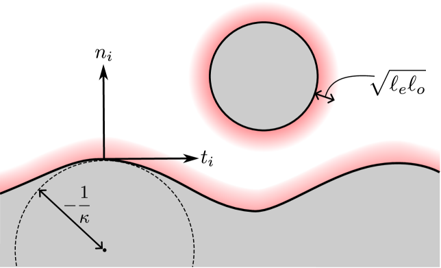
Figure 2: An example geometry with the flow domain shown in white and boundaries is gray. The sample edge is described by a local curvature $\kappa$ and boundary normal and tangent unit vectors $n_{i}$ and $t_{i}$, respectively. The approximate extent of the anomalously large tomographic boundary layer is indicated by a red shaded region.

Our solution to the kinetic equation in this limit reveals four striking phenomena for tomographic flows: First, sufficiently far from the diffuse edges (which we term the bulk region), the flow is described by Stokes-Ohm like equations with higher-order derivative terms associated with rarefaction effects. Second, the boundary conditions for these bulk equations a exhibit striking deviation from the widely-used slip-length velocity boundary conditions. In particular, the leading-order velocity slip condition for the bulk flow is found to depend on the local curvature of the device edge and the applied magnetic field strength. Third, near any diffuse edge, a kinetic boundary layer of thickness $\sim\sqrt{\ell_{e}\ell_{o}}$ arises (which we term the “tomographic boundary layer”), where the flow is not described by the above-mentioned bulk equations (see Fig. 2). Last, all of the above-mentioned phenomena are found to be strongly suppressed by an applied magnetic field, from which the relaxation of the odd-modes can be easily extracted.

In more detail, in this work we consider a kinetic equation with separate relaxation rates for the distribution function’s even and odd-modes, as well as an additional rate of momentum-relaxing scattering [26]. In dimensionless form,

$$v_{i}\frac{\partial h}{\partial x_{i}}+2k_{e}v_{i}E_{i}-\frac{1}{r_{c}}v_{i}^{\perp}\frac{\partial h}{\partial v_{i}}$$

$$=-\frac{1}{k_{e}}\left(\left[h\right]_{e}-\delta\mu\right)-\frac{1}{k_{o}}\left(\left[h\right]_{o}-2v_{i}u_{i}\right)-\frac{k_{e}}{G^{2}}\left(h-\delta\mu\right).$$ (5)

This is the main equation that we will analyze in this paper for arbitrary geometries with diffusive boundary conditions, where the even and odd components of the distribution function $\left[h\right]_{e}$ and $\left[h\right]_{o}$ are given in Eqs. (1) and (2). For a derivation of Eq. (5) from the electron Boltzmann equation, we refer to App. A. In Eq. (5), the spatial and velocity coordinates, $x_{i}$ and $v_{i}$, are respectively scaled by the macroscopic length scale, $L$, and the Fermi velocity, $v_{F}$. The dimensionless electric field $E_{i}$ unit vector has been scaled by the magnitude of the applied electric field, $\mathcal{E}$. In addition, the distribution function $h$ describes the local deformation of the Fermi surface at the point $x_{i}$, which is parameterized by the orientation $\theta$ of the velocity $v_{i}$ vector. Macroscopic variables are obtained as moments of the distribution function, with the scaled non-equilibrium electrochemical potential

$$\delta\mu=\int_{-\pi}^{\pi}\frac{d\theta}{2\pi}\,h,$$ (6)

and mean velocity

$$u_{i}=\int_{-\pi}^{\pi}\frac{d\theta}{2\pi}\,(v_{i}h),$$ (7)

which are scaled by the hydrodynamic scales for electric field driven flows, $e\mathcal{E}L$ and $e\mathcal{E}L^{2}/(v_{F}\ell_{e}m^{*})$, respectively, where $e$ is the fundamental charge, $m^{*}$ is the effective mass of the electrons. The left-hand side of the kinetic Eq. (5) is the streaming term. It contains an advective term, and we also include both external electric and magnetic fields, where we introduce the shorthand $v_{i}^{\perp}=\varepsilon_{ij}v_{j}$ and the scaled cyclotron radius

$$r_{c}=\frac{m^{*}v_{F}}{e\mathcal{B}L}=\frac{R_{c}}{L},$$ (8)

where $\cal B$ is the strength of the applied magnetic field, and $R_{c}$ is the dimensional cyclotron radius.

The right-hand side of Eq. (5) is the key departure from a conventional description of hydrodynamic transport and models collisions beyond the dual-relaxation time approximation. Here, the first term describes the relaxation by electron-electron collisions of even modes with even-mode Knudsen number $k_{e}\ll 1$ [cf. Eq. (3)], where the subtraction excludes the density zero mode. The second term in Eq. (5) describes the electronic relaxation of odd modes with a characteristic odd-mode Knudsen number

$$k_{o}=\frac{\ell_{o}}{L},$$ (9)

which, by Eq. (4), is of order unity, in contrast to the even-mode Knudsen number $k_{e}$. The third term in Eq. (5) accounts for momentum-relaxing processes that are parameterized by the Gurzhi number

$$G=\frac{\sqrt{\ell_{e}\ell_{\text{MR}}}}{L}.$$ (10)

Restating the length scale separation in Eq. (4) in terms of the even and odd-mode Knudsen numbers as well as the Gurzhi number gives

$$k_{e}\ll 1\lesssim G\sim k_{o}.$$ (11)

Equation (5) must be solved with appropriate boundary conditions on the microscopic distribution function. Diffuse boundary conditions constrain the distribution of states that are reflected at the surface [i.e., which have a velocity component that points into the flow domain, $v_{i}n_{i}>0$, cf. Fig. 2] as

$$\bigl{[}h(v_{i})\bigr{]}_{S}=-\frac{1}{2}\int_{v_{i}n_{i}<0}d\theta\,(v_{i}n_{i})\bigl{[}h(v_{i})\bigr{]}_{S},$$ (12)

where the subscript $S$ indicates that the distribution is evaluated at the edge. This boundary condition expresses that the distribution for all reflected velocities $v_{i}n_{i}>0$ is completely randomized and hence isotropic. The choice of the right-hand side of Eq. (12) ensures that the velocity component (7) normal to the edge vanishes, i.e., that there is no penetration through the boundary.

The remainder of the paper is structured as follows: We begin in Sec. II with an overview that summarizes our key findings. These include a list of governing equations for the mean velocity and electrochemical potential, their boundary conditions, and tomographic boundary layer corrections. These equations are the fundamental equations for tomographic flow and constitute the central result of or work. They are valid for flow in arbitrary devices with a smooth edge geometry. Section III provides a detailed derivation of the asymptotic solution to the governing kinetic equation (5), which gives the above-mentioned bulk equations, boundary conditions and tomographic boundary layer corrections. We illustrate the use of the asymptotic theory by solving for the flow in a channel in Sec. IV, discussed in detail in Ref. [27], which provides extended results on the flow profile and the Fermi surface deformation. The paper concludes with a summary and outlook in Sec. V. Details of some calculations are relegated to four appendices.

II Summary of results

We begin by summarizing and discussing the asymptotic theory for tomographic flows. As illustrated in Fig. 2, the flow domain is split in a bulk region and a boundary layer region (red shaded area). In the bulk region the flow is dominated by collisions that establish a local equilibrium, giving a hydrodynamic-like “bulk” flow. As we shall show, this bulk flow is governed by Stokes-Ohm like equations with higher-order derivative corrections. Such corrections become important in any form of confinement where the flow profile is no longer uniform. However, diffuse scattering at device edges prevents the establishment of a local equilibrium at the boundary. This gives rise, first, to a kinetic boundary layer near any diffuse edge, over which the non-equilibrium distribution function at the boundary relaxes to toward the equilibrium distribution function in the bulk, and, second, it introduces modified slip boundary condition on the bulk flow. For tomographic flows, we find that the kinetic boundary layer extends over the anomalously large characteristic tomographic length scale $\sqrt{\ell_{e}\ell_{o}}$ [26, 16, 18], which arises from the balance of even-mode induced diffusion and odd-mode collisions. Thus, we term this boundary layer the “tomographic boundary layer”.

The $O(\sqrt{\ell_{e}\ell_{o}})$ width of the tomographic boundary layer requires the distribution function and each of its moments to be expanded in powers of the nonanalytic parameter $\sqrt{k_{e}}$,

$$\Psi=\Psi^{(0)}_{B}+\sqrt{k_{e}}\Psi^{(1)}_{B}+k_{e}\left(\Psi^{(2)}_{B}+\Psi^{(2)}_{T}\right)+\dots.$$ (13)

Here, $\Psi\in\{h,\delta\mu,u_{i}\}$ is each of the dependent variables [cf. Sec. 1 of Tab. 1], and the subscripts “B” and “T”, respectively, correspond to the solution in the bulk and the correction in the tomographic boundary layer (see Fig. 2). In the bulk, the macroscopic variables (i.e., $\delta\mu_{B}$ and $u_{B|i}$) satisfy coupled governing equations at each order of expansion in $\sqrt{k_{e}}$, which are listed up to ${\it O}(k_{e})$ in Sec. 2 of Tab. 1. The appropriate boundary conditions for these bulk equations at diffuse edges are listed in Sec. 3 of Tab. 1. In addition, starting at order ${\it O}(k_{e})$, the microscopic diffuse boundary condition can only be satisfied with a tomographic boundary layer, which gives a correction to the macroscopic variables at this order; see Sec. 4 of Tab. 1.

1.  Asymptotic expansion
$$\begin{array}[]{rl}&\displaystyle\delta\mu=\delta\mu_{B}^{(0)}+\sqrt{k_{e}}\,\delta\mu_{B}^{(1)}+k_{e}\left(\delta\mu_{B}^{(2)}+\delta\mu_{T}^{(2)}\right)+\dots\\[4.30554pt] &\displaystyle u_{i}=u_{B|i}^{(0)}+\sqrt{k_{e}}\,u_{B|i}^{(1)}+k_{e}\left(u_{B|i}^{(2)}+u_{T|i}^{(2)}\right)+\dots\end{array}$$ (14)
2.  Bulk equations
Incompressibility condition: $\displaystyle\displaystyle\frac{\partial u_{B|i}^{(n)}}{\partial x_{i}}=0,\quad n\geq 0,$ (15a) Tomographic Stokes-Ohm equations: $\displaystyle\displaystyle-\frac{1}{2}\frac{\partial\delta\mu^{(n)}_{B}}{\partial x_{i}}=$ $\displaystyle\displaystyle\frac{1}{r_{c}}\varepsilon_{ij}u_{B|j}^{(n)},\hskip 22.0ptn\in\{0,1\},$ (15b) $\displaystyle\displaystyle-\frac{1}{2}\frac{\partial\delta\mu_{B}^{(2)}}{\partial x_{i}}=$ $\displaystyle\displaystyle\frac{u_{B|i}^{(0)}}{G^{2}}-\frac{1}{4}\frac{\partial^{2}u_{B|i}^{(0)}}{\partial x_{j}^{2}}+\frac{1}{r_{c}}\varepsilon_{ij}u_{B|j}^{(2)}+E_{i},$ (15c) $\displaystyle\displaystyle-\frac{1}{2}\frac{\partial\delta\mu_{B}^{(3)}}{\partial x_{i}}=$ $\displaystyle\displaystyle\frac{u_{B|i}^{(1)}}{G^{2}}-\frac{1}{4}\frac{\partial^{2}u_{B|i}^{(1)}}{\partial x_{j}^{2}}+\frac{1}{r_{c}}\varepsilon_{ij}u_{B|j}^{(3)},$ (15d) $\displaystyle\displaystyle-\frac{1}{2}\frac{\partial\delta\mu_{B}^{(4)}}{\partial x_{i}}=$ $\displaystyle\displaystyle\frac{u_{B|i}^{(2)}}{G^{2}}-\frac{1}{4}\frac{\partial^{2}u_{B|i}^{(2)}}{\partial x_{j}^{2}}+\frac{1}{r_{c}}\varepsilon_{ij}u_{B|j}^{(4)}+\frac{1}{2r_{c}}\varepsilon_{ij}\frac{\partial^{2}u_{B|j}^{(0)}}{\partial x_{k}^{2}}-\frac{k_{o}}{16(1+(3k_{o}/r_{c})^{2})}\biggl{(}\frac{\partial^{4}u_{B|i}^{(0)}}{\partial x_{k}^{2}\partial x_{l}^{2}}-\frac{3k_{o}}{r_{c}}\varepsilon_{ij}\frac{\partial^{4}u_{B|j}^{(0)}}{\partial x_{k}^{2}\partial x_{l}^{2}}\biggr{)}.$ (15e)
3.  Boundary conditions
No-penetration: $\displaystyle\Bigl{[}u_{B|i}^{(0)}n_{i}\Bigr{]}_{S}$ $\displaystyle=0,\qquad\Bigl{[}u_{B|i}^{(1)}n_{i}\Bigr{]}_{S}=0,\qquad\Bigl{[}u_{B|i}^{(2)}n_{i}\Bigr{]}_{S}=0,$ (16a) No-slip/tomographic slip: $\displaystyle\Bigl{[}u_{B|i}^{(0)}t_{i}\Bigr{]}_{S}=0,\qquad$ $\displaystyle\Bigl{[}u_{B|i}^{(1)}t_{i}\Bigr{]}_{S}=0,$ (16b) $\displaystyle\displaystyle\Bigl{[}u_{B|i}^{(2)}t_{i}\Bigr{]}_{S}=\displaystyle-\frac{32}{15\pi}\Bigl{[}n_{i}t_{j}S_{B|ij}^{(0)}\Bigr{]}_{S}-\frac{k_{o}}{2(1+(3k_{o}/r_{c})^{2})}\Biggl{(}\kappa\Bigl{[}n_{i}t_{j}$ $\displaystyle S_{B|ij}^{(0)}\Bigr{]}_{S}-\frac{1}{2}\biggl{[}t_{i}n_{j}n_{k}\frac{\partial S_{B|ij}^{(0)}}{\partial x_{k}}\biggr{]}_{S}+\frac{9}{4}\frac{k_{o}}{r_{c}}\biggl{[}n_{i}n_{j}n_{k}\frac{\partial S_{B|ij}^{(0)}}{\partial x_{k}}\biggr{]}_{S}\Biggr{)}.$ (16c)
4.  Tomographic boundary layer
Rescaled tomographic boundary layer normal coordinate: $\displaystyle\hskip 56.9055pt\chi=\frac{x_{i}n_{i}}{\sqrt{k_{e}k_{o}}}.$ (17a) Tomographic boundary layer corrections: $\displaystyle u_{T|i}^{(2)}n_{i}$ $\displaystyle=0,$ (17b) $\displaystyle\displaystyle u_{T|i}^{(2)}t_{i}$ $\displaystyle=\displaystyle\mathcal{Y}_{0}(\chi;\tfrac{k_{o}}{r_{c}})\Bigl{[}n_{i}t_{j}S_{B|ij}^{(0)}\Bigr{]}_{S}+k_{o}\mathcal{Y}_{1}(\chi;\tfrac{k_{o}}{r_{c}})\kappa\Bigl{[}n_{i}t_{j}S_{B|ij}^{(0)}\Bigr{]}_{S}-\frac{k_{o}}{2}\mathcal{Y}_{1}(\chi;\tfrac{k_{o}}{r_{c}})\biggl{[}t_{i}n_{j}n_{k}\frac{\partial S_{B|ij}^{(0)}}{\partial x_{k}}\biggr{]}_{S}+k_{o}\mathcal{Y}_{2}(\chi;\tfrac{k_{o}}{r_{c}})\biggl{[}n_{i}n_{j}n_{k}\frac{\partial S_{B|ij}^{(0)}}{\partial x_{k}}\biggr{]}_{S},$ (17c) $\displaystyle\delta\mu_{T}^{(2)}$ $\displaystyle=0,$ (17d) $\displaystyle\displaystyle\frac{\partial\delta\mu_{T}^{(3)}}{\partial\chi}$ $\displaystyle=\displaystyle\frac{2\sqrt{k_{o}}}{r_{c}}u_{T|i}^{(2)}t_{i}+\frac{1}{\sqrt{k_{o}}}\mathcal{T}_{0}(\chi;\tfrac{k_{o}}{r_{c}})\Bigl{[}n_{i}t_{j}S_{B|ij}^{(0)}\Bigr{]}_{S}+\sqrt{k_{o}}\mathcal{T}_{1}(\chi;\tfrac{k_{o}}{r_{c}})\kappa\Bigl{[}n_{i}t_{j}S_{B|ij}^{(0)}\Bigr{]}_{S}-\frac{\sqrt{k_{o}}}{2}\mathcal{T}_{1}(\chi;\tfrac{k_{o}}{r_{c}})\biggl{[}t_{i}n_{j}n_{k}\frac{\partial S_{B|ij}^{(0)}}{\partial x_{k}}\biggr{]}_{S}$ $\displaystyle\quad\displaystyle+\sqrt{k_{o}}\mathcal{T}_{2}(\chi;\tfrac{k_{o}}{r_{c}})\biggl{[}n_{i}n_{j}n_{k}\frac{\partial S_{B|ij}^{(0)}}{\partial x_{k}}\biggr{]}_{S}.$ (17e)

Table 1: Summary of the tomographic flow equations: (1) The electrochemical potential and the flow velocity are expanded in powers of $\sqrt{k_{e}}$ with the small Knudsen number $k_{e}\ll 1$. The expansion consists of a bulk contribution (subscript “B”) and, at order ${\it O}(k_{e})$, a tomographic boundary layer contribution (subscript “T”); (2) The governing equations for the bulk macroscopic variables obey incompressibility and the “tomographic Stokes-Ohm” equations. Equation (15e) includes tomographic higher-derivative corrections that are of the same order as the Hall viscosity correction; (3) Boundary conditions for the bulk flow equations listed in (2) for diffuse microscopic boundary scattering. $S_{B|ij}^{(n)}$ is the rate-of-strain tensor in the bulk region [Eq. (19)], and $\kappa$ is the local curvature of the boundary. All bulk quantities are evaluated at the boundary; (4) Tomographic boundary layer corrections to the velocity, $u_{T|i}^{(n)}$, and Hall field, $\partial\delta\mu_{T}^{(n)}/\partial\chi$, up to order ${\it O}(k_{e})$. The tomographic boundary layer functions $\mathcal{Y}_{0}$, $\mathcal{Y}_{1}$, $\mathcal{Y}_{2}$, $\mathcal{T}_{o}$, $\mathcal{T}_{1}$, and $\mathcal{T}_{2}$ are independent of the geometry and evaluated in App. C and plotted in Fig. 4.

In Tab. 1, the geometry of the boundary, which is assumed arbitrary and smooth in this study, is described by a unit normal ($n_{i}$) and unit tangent ($t_{i}$) vectors (see Fig. 2). These satisfy the general geometric relations [28]

$$n_{j}\frac{\partial n_{i}}{\partial x_{j}} =0, n_{j}\frac{\partial t_{i}}{\partial x_{j}} =0,$$ (18a)

$$t_{j}\frac{\partial n_{i}}{\partial x_{j}} =\kappa t_{i}, t_{j}\frac{\partial t_{i}}{\partial x_{j}} =-\kappa n_{i},$$ (18b)

where $\kappa$ is the local (scaled) curvature of the edge, which is defined to be negative when its center of curvature lies in the electron flow domain. In addition, we define the rate-of-strain tensor at each order

$$S_{B|ij}^{(n)}=-\biggl{(}\frac{\partial u_{B|i}^{(n)}}{\partial x_{j}}+\frac{\partial u_{B|j}^{(n)}}{\partial x_{i}}\biggr{)}.$$ (19)

The bulk governing equations, their boundary conditions, and tomographic boundary layer corrections listed in Tab. 1 are the main result of this study. They form a complete asymptotic theory of tomographic electron flow up to ${\it O}(k_{e})$, which captures phenomena beyond the hydrodynamic limit, and which may be utilized to calculate the flow in any device with smooth boundary geometry up to linear order for $k_{e}\ll 1$ (including those with curved boundaries and with an applied perpendicular magnetic field). Thus, they provide an alternative to computationally expensive numerical solutions of the kinetic equation for electron flows at small $k_{e}$, and they also provide crucial analytical insight into the flow structure. Moreover, the microscopic distribution function is expressed in terms of the macroscopic variables in Tab. 2, and thus a solution for the macroscopic variables allows to reconstruct the full distribution function. We next describe key properties of the asymptotic theory, which are embodied in the bulk governing equations [Sec. II.1], their boundary conditions [Sec. II.2], the tomographic boundary layer corrections [Sec. II.3], and the reconstructed electron distribution function [Sec. II.4], and we briefly summarize how these equations should be solved for a given geometry [Sec. II.5].

1.  Asymptotic expansion
$$\displaystyle h=h_{B}^{(0)}+\sqrt{k_{e}}h_{B}^{(1)}+k_{e}\left(h_{B}^{(2)}+h_{T}^{(2)}\right)+\dots$$ (20)
2.  Bulk
$\displaystyle h^{(n)}_{B}$ $\displaystyle=\delta\mu^{(n)}_{B}+2v_{i}u_{B|i}^{(n)},\quad n\in\{0,1\},$ (21a) $\displaystyle h^{(n)}_{B}$ $\displaystyle=\delta\mu^{(n)}_{B}+2v_{i}u_{B|i}^{(n)}-2v_{i}v_{j}\frac{\partial u_{B|i}^{(n-2)}}{\partial x_{j}}$ $\displaystyle\hskip-10.00002pt+\frac{\partial^{2}u_{B|i}^{(n-2)}}{\partial x_{j}\partial x_{k}}\Bigg{[}\frac{2k_{o}}{1+(3k_{o}/r_{c})^{2}}\left(v_{i}v_{j}v_{k}-\frac{1}{4}v_{i}\delta_{jk}\right)$ $\displaystyle\hskip-10.00002pt-\frac{6k_{o}^{2}/r_{c}}{1+(3k_{o}/r_{c})^{2}}\left(v_{i}^{\perp}v_{j}^{\perp}v_{k}^{\perp}-\frac{1}{4}v_{i}^{\perp}\delta_{jk}\right)\Bigg{]},\quad n\in\{2,3\}.$ (21b) 3.  Tomographic boundary layer correction
$\displaystyle h_{T}^{(2)}$ $\displaystyle=f_{0}(\chi,\theta;\tfrac{k_{o}}{r_{c}})\Bigl{[}n_{i}t_{j}S_{B|ij}^{(0)}\Bigr{]}_{S}$ $\displaystyle\quad+f_{1}(\chi,\theta;\tfrac{k_{o}}{r_{c}})k_{o}\kappa\Bigl{[}n_{i}t_{j}S_{B|ij}^{(0)}\Bigr{]}_{S}$ $\displaystyle\quad-\frac{1}{2}f_{1}(\chi,\theta;\tfrac{k_{o}}{r_{c}})k_{o}\biggl{[}t_{i}n_{j}n_{k}\frac{\partial S_{B|ij}^{(0)}}{\partial x_{k}}\biggr{]}_{S}$ $\displaystyle\quad+f_{2}(\chi,\theta;\tfrac{k_{o}}{r_{c}})k_{o}\biggl{[}n_{i}n_{j}n_{k}\frac{\partial S_{B|ij}^{(0)}}{\partial x_{k}}\biggr{]}_{S}.$ (22) Tomographic equation:
$\displaystyle(v_{i}n_{i})^{2}\frac{\partial^{2}h_{T}^{(2)}}{\partial\chi^{2}}-h_{T}^{(2)}+\frac{k_{o}}{r_{c}}v_{k}^{\perp}\frac{\partial h_{T}^{(2)}}{\partial v_{k}}$ $\displaystyle\quad=-2v_{i}t_{i}u_{T|j}^{(2)}t_{j}+\sqrt{k_{o}}v_{i}n_{i}\frac{\partial\delta\mu_{T}^{(3)}}{\partial\chi}.$ (23)

Table 2: Microscopic distribution function $h_{B}^{(n)}$ at each order of the asymptotic expansion, and its ${\it O}(k_{e})$ correction in the tomographic boundary layer, $h_{T}^{(2)}$. The functions $f_{0}$, $f_{1}$ and $f_{2}$ are independent of the geometry and solved numerically in App. C.

II.1 Bulk governing equations

We begin by describing the bulk governing equations for the Hall field and the velocity profile, which are summarized in Eqs. (15) in Tab. 1. The first set of constraint equations [Eq. (15a)] enforces a divergence-free bulk velocity at all orders in $k_{e}$, corresponding to incompressible electron flow in spite of generalized relaxation times. The second set of constraint equations [Eqs. (15b)-(15e)] describe macroscopic momentum transport, and include both the Hall field ($-\partial\delta\mu_{B}/\partial x$) and the velocity profile. While in conventional hydrodynamics, these latter equations are the standard Stokes-Ohm equations, we find here that such a description is no longer valid in general and is modified by higher-derivative corrections:

First, only at leading order in the Knudsen number $k_{e}\ll 1$ do we obtain the widely-used Stokes-Ohm equations [Eqs. (15b)-(15d)]. These are characterized by a balance of drag from residual momentum-relaxing collisions, shear viscous forces, the magnetic force and the electric field. From the third term in Eq. (15c), we read off the (dimensional) shear viscosity of the electron fluid $v_{F}\ell_{e}/4$ [29, 30], and a Hall viscosity term does not arise at this order in the Knudsen number. The appearance of the Stokes-Ohm equation is a consequence of a local equilibrium being established to leading-order in the bulk.

Second, at order ${\it O}(k_{e})$, the Hall viscosity arises in the bulk equations [the second-to-last term $\varepsilon_{ij}\partial^{2}u_{B|j}^{(0)}/\partial x_{k}^{2}$ term in Eq. (15e)]. This corresponds to the well-known dimensional Hall viscosity of $v_{F}\ell_{e}^{2}/(2R_{c})$ [29, 30]. However, at the same order previously unreported finite-wavelength corrections (i.e., rarefaction phenomena) are also found in the bulk equation in the form of higher-derivative terms $\partial^{4}/\partial^{2}x_{k}\partial^{2}x_{l}$ [the last term in round brackets in Eq. (15e)]. These corrections are linear in the odd-mode Knudsen number $k_{o}$ and are thus directly associated with the long-lived odd-modes of the distribution function. These terms are of equal order and magnitude as the Hall viscosity. For example, for a channel-flow type geometry with a bulk velocity in the $y$-direction that varies in the $x$-direction and an external magnetic field in the $z$-direction, Eq. (15) dictates that the Hall field ($-\partial\delta\mu_{B}/\partial x$) is related to the velocity profile via,

$$-\frac{\partial\delta\mu_{B}}{\partial x}= \frac{2}{r_{c}}\left[u_{y}+\frac{k_{e}^{2}}{2}\left(1+\frac{3k_{o}^{2}}{2G^{2}}\frac{1}{1+(3k_{o}/r_{c})^{2}}\right)\frac{\partial^{2}u_{B|y}}{\partial x^{2}}\right]$$

$$+{\it o}(k_{e}^{2}).$$ (24)

The first term in the square brackets is the (continuum) Lorentz force contribution, while the second term (with prefactor $k_{e}^{2}$) gives the leading-order rarefaction correction to the bulk Hall field. Interestingly, this correction is strongly dependent on the magnetic field, where the first term in the round brackets is the usual Hall viscosity contribution [24, 25, 31], while the second term—which is of the same order—is a new contribution associated with the tomographic effect. Thus, in this flow regime, the deviation of the Hall field from Lorentz force predictions is not given by the Hall viscosity alone. Moreover, the tomographic contribution to Eq. (24) depends on the magnetic field strength, following a Lorentzian of width $3k_{o}/r_{c}=3\ell_{o}/R_{c}$, and is suppressed at relatively moderate magnetic fields for which $r_{c}\sim 1/(3k_{o})$, i.e., when the cyclotron radius is comparable to the large odd-mode mean free path. The suppression of the tomographic contribution to Eq. (24) gives a simple method for determining the odd-mode mean free path: For sufficiently large magnetic field strengths (i.e., for which $R_{c}<\ell_{o}$), the tomographic correction is suppressed and Eq. (24) recovers a hydrodynamic prediction, where the contribution from the tomographic effect vanishes.

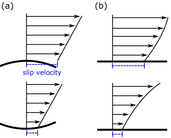
Figure 3: Schematic showing the tomographic effect on the slip velocity boundary condition (blue dashed line) of (a) the boundary curvature and (b) the bulk flow profile (solid black arrows), as dictated by Eq. (16c). We indicate boundaries as thick black lines and show bulk flows with equal shear rate (i.e., equal slope at the boundary). Panel (a) shows the dependence on the boundary curvature, with a convex boundary increasing the slip (top panel) and decreasing it for a concave boundary (bottom panel). Panel (b) illustrates the dependence of the slip condition on the curvature of the boundary flow, with a negative curvature increasing (top panel) and positive curvature decreasing (bottom panel) the slip. In all panels, we draw only the bulk flow, and the full asymptotic velocity profile, which includes the tomographic layer corrections, is not sketched. The figures illustrates that the increased range of the tomographic boundary region due to the admixture of ballistic odd modes induces an additional dependence of the slip condition on both the bulk flow profile and the boundary structure, which is not found for conventional hydrodynamic flows at leading order.

II.2 Boundary conditions on the bulk solution

The bulk governing equations (15) for $\delta\mu_{B}$ and $u_{B}$ must be solved with appropriate boundary conditions, which follow from the microscopic diffuse boundary condition (12) on the distribution function. The velocity-slip boundary conditions for the bulk governing equations obtained in this way are summarized in Eq. (16) of Tab. 1. The diffuse boundary scattering (12) imposes a no-penetration boundary condition [Eq. (16a)] on the normal component of the velocity up to $O(k_{e})$, which prevents flow through the boundaries. The remainder of the discussion therefore focuses on the boundary condition for the tangential component of the velocity (i.e., which gives rise to velocity slip).

First, at leading order ${\it O}(1)$ and ${\it O}(\sqrt{k_{e}})$ (i.e., for $u_{B}^{(0)}$ and $u_{B}^{(1)}$), we obtain no-slip boundary conditions [Eq. (16b)] as is normally associated with diffuse reflection in the hydrodynamic limit [2]. This is attributed to collisions establishing a local equilibrium throughout the spatial domain at these orders in $k_{e}$. Since diffuse reflection forces the reflected electrons into equilibrium with the edge, this requires the no-slip condition for the hydrodynamic equations.

Second, by contrast, at ${\it O}(k_{e})$, (i.e., for $u_{B}^{(2)}$), slip conditions arise [Eq. (16c)]. Strikingly, the leading-order tomographic slip boundary condition for the bulk equations strongly deviate from the widely-used slip-length boundary conditions of hydrodynamic flow [32, 33, 34, 2, 35]. In particular, the slip velocity condition is induced by (i) the shear-stress of the leading-order flow (this gives the usual slip-length condition) [first term in Eq. (16c)], (ii) the local curvature of the boundary [second term in Eq. (16c)], (iii) the boundary-normal gradient in the shear-stress [third term in Eq. (16c)], and (iv) the boundary-normal gradient in the normal-stress [fourth term in Eq. (16c)], where the rate-of-strain tensor is defined in Eq. (19). The coefficient $32/(15\pi)\approx 0.679$ of $S_{B|ij}^{(0)}n_{i}t_{j}$ in the first term of Eq. (16c) (which gives the slip-length condition) is approximately 7% larger than the slip coefficient found for conventional hydrodynamic flows of $0.6366\dots$ [35]. Furthermore, the latter three contributions are directly associated with the tomographic effect; they do not arise in the leading-order slip boundary conditions of conventional hydrodynamic flows [24, 25]. The last contribution arises in the presence of an applied magnetic field only. Schematics of the slip condition predicted by Eq. (16c) are shown in Fig. 3. In particular, Fig. 3(a) Fig. 3(b) illustrates the effects of the boundary curvature on the slip [third term in Eq. (16c)], and shows the effects of curvature in the bulk flow velocity at the boundary on the slip [second term in Eq. (16c)]. Compared with the widely-used fixed slip-length condition, the second contribution enhances the slip for concave boundaries and suppresses it for convex boundaries. The tomographic contributions to the slip condition in Eq. (16c) are found to be rapidly suppressed by a magnetic field, and decrease in magnitude as a Lorentzian of width $3\ell_{o}/R_{c}$. Together, these phenomena demonstrate that the use of the fixed slip-length boundary condition is inadequate for modeling near-continuum flows that exhibit the tomographic effect.

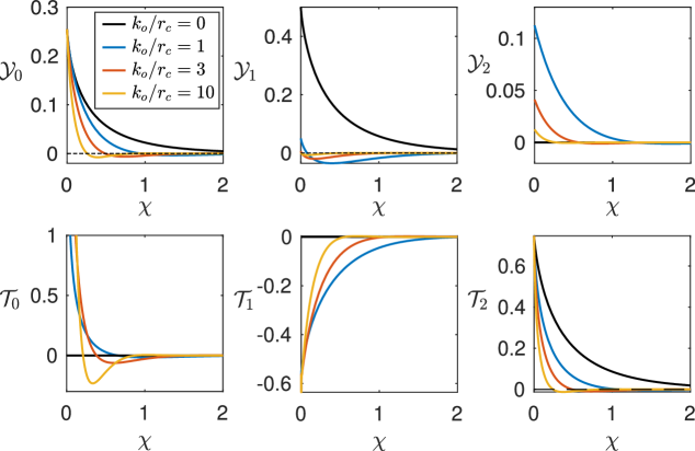
Figure 4: Tomographic boundary layer functions for the velocity, $\mathcal{Y}_{0}$, $\mathcal{Y}_{1}$ and $\mathcal{Y}_{2}$, and for the Hall field, $\mathcal{T}_{0}$, $\mathcal{T}_{1}$ and $\mathcal{T}_{2}$, as a function of the rescaled spatial coordinate $\chi=x/\sqrt{k_{e}k_{o}}$, for $k_{o}/r_{c}\in\{0,1,3,10\}$. The dashed line marks $0$.

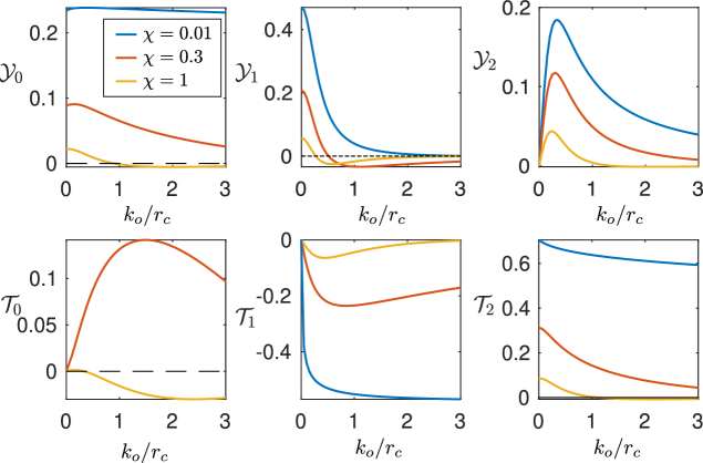
Figure 5: Same as Fig. 4, but as a function of $k_{o}/r_{c}$, for $\chi\in\{0,0.3,1\}$. The dashed line marks $0$. The function $\mathcal{T}_{0}$ diverges for $\chi\to 0^{+}$ and thus is not plotted at $\chi=0$.

II.3 Tomographic boundary layer corrections

The tomographic boundary layer extends over the (dimensional) length scale $\sqrt{\ell_{e}\ell_{o}}$. It thus covers a significantly larger proportion of the flow domain compared with the Knudsen boundary layer that arises in classical hydrodynamic electron flows, which extends over a much shorter length scale $\ell_{e}$. As we shall show, the leading-order distribution function in the tomographic boundary layer satisfies Eq. (2), which is characterized by a balance of even-mode induced diffusion, odd-mode collisions, and the magnetic force. Equation (2) possesses an identical structure to Eq. (10) of [17] with $p=0$, thus giving the tomographic boundary layer its name. Tomographic boundary layer corrections are found at ${\it O}(k_{e})$ for the distribution function, velocity profile and Hall profile (indicated with a subscript “T”), which must be added to the bulk solution. The tomographic boundary layer correction for the velocity and Hall profiles are listed in Eq. (17) of Tab. 1, while the from of the tomographic boundary layer correction for the distribution function is listed in Tab. 2. Their structure is similar to that of the velocity-slip condition for the bulk solution [Eq. (16c)]. The functions $\mathcal{Y}_{0}$, $\mathcal{Y}_{1}$, $\mathcal{Y}_{2}$, $\mathcal{T}_{0}$, $\mathcal{T}_{1}$, and $\mathcal{T}_{2}$, which are termed tomographic boundary layer functions, depend on the magnetic field through the ratio of the odd-mode mean free path to the cyclotron radius. Solution for these are shown in Figs. 4 and 5.

Interestingly, all tomographic boundary layer functions become confined near the boundary when the magnetic field strength is increased, and for $R_{c}<\ell_{o}$, the boundary layer extends over the (dimensional) length scale $\sqrt{\ell_{e}R_{c}}<\sqrt{\ell_{e}\ell_{o}}$. The tomographic boundary layer corrections to the Hall field ($\mathcal{T}_{0}$, $\mathcal{T}_{1}$ and $\mathcal{T}_{2}$) exhibit non-monotonic behavior with respect to the magnetic field strength (see Fig. 5). These tomographic boundary layer corrections contribute significantly to the electrochemical potential at the device edges, and thus dictate measurable properties of the flow, e.g., the Hall resistance.

II.4 Full electron distribution function

Once the macroscopic variables, i.e., the velocity $u_{i}$ and the Hall field $-\partial\delta\mu/\partial x_{i}$ are known, it is straightforward to reconstruct the full Fermi surface deformation function $h$. This is summarized in Tab. 2 up to linear order ${\it O}(k_{e})$ of the Knudsen number, where the deformation is expanded in powers of the Knudsen number as shown in Eq. (13) or Eq. (20) of Tab. 2. We will discuss the structure of these equations next.

The leading-order deformations at $O(k_{e}^{0})$ and $O(k_{e}^{1/2})$ are set by the bulk solution at this order, Eq. (21a) of Tab. 2. They consist of a uniform change in the electrochemical potential that describes a local change in the electron density, as well as a current contribution that displaces the center of mass of the Fermi surface. These are exactly the microscopic deformations that describe hydrodynamic degrees of freedom.

This simple structure of the deformation is modified at ${\it O}(k_{e})$ and higher: The bulk contribution [Eq. (21) of Tab. 2] now contains an additional even-parity deformation that is proportional to the rate-of-strain tensor [the third term in Eq. (21)], as well as an odd-parity deformation that is proportional to the curvature of the velocity profile [the last term in square brackets in Eq. (21)]. Microscopically, the even-parity term contributes to a Fermi surface deformation with an angular-mode dependence proportional to $\cos(2\theta)$ or $\sin(2\theta)$, i.e., the Fermi surface takes quadrupolar form that is squeezed along one axis in momentum space but elongated in another. This is a microscopic shear deformation, which is induced by even-mode collisions [36]. By contrast, the odd-parity deformations are of the tetragonal form $\cos(3\theta)$ or $\sin(3\theta)$. Restoring powers of the Knudsen number, they are ${\it O}(k_{e}k_{o})$, and thus induced by repeated odd- and even-mode collisions.

It is not correct, however, to assume that the harmonic expansion truncates at the third harmonic order. Higher deformations enter in the tomographic boundary layer, which also contributes at ${\it O}(k_{e})$ [Eq. (2) of Tab. 2]. These corrections depend on the tomographic layer functions $f_{0},f_{1}$ and $f_{2}$, which solve the tomographic equation (2). They are evaluated explicitly in App. C using a truncated moment expansion in terms of coefficients that describe the projection onto the angular harmonic modes of the deformation. This analysis shows that the diffusive boundary scattering induces a Fermi surface deformation that strongly deviates from the hydrodynamic form and involves a large number of higher angular modes.

II.5 Solving the asymptotic equations

An analytical or numerical solution of the asymptotic theory listed in Tab. 1 proceeds as follows: First, the bulk governing equations for the leading order velocity $u_{B|i}^{(0)}$ [Eqs. (15a) and (15c)] are solved subject to the no-slip condition at device edges. Depending on the geometry of the device edges, this can be obtained by direct integration (this procedure is shown for channel flow in Sec. IV) or other standard techniques in simple geometries. One such technique is the stream-function formulation [37], which we describe next applied to solve the asymptotic theory.

The incompressibility condition [Eq. (15a)] permits expressing the bulk velocity in terms of a stream function,

$$u_{B|i}^{(0)}=\varepsilon_{ij}\frac{\partial\psi^{(0)}}{\partial x_{j}}.$$ (25)

Then taking the curl of Eq. (15c) furnishes an equation for $\psi^{(0)}$,

$$\frac{1}{G^{2}}\frac{\partial^{2}\psi^{(0)}}{\partial x_{i}^{2}}-\frac{1}{4}\frac{\partial^{4}\psi^{(0)}}{\partial x_{i}^{2}\partial x_{j}^{2}}+\varepsilon_{ij}\frac{\partial E_{i}}{\partial x_{j}}=0.$$ (26)

The no-slip and no-penetration condition at the device edges then become

$$\left[\psi^{(0)}\right]_{S}=0,\qquad\left[n_{i}\frac{\partial\psi^{(0)}}{\partial x_{i}}\right]_{S}=0,$$ (27)

which can be used to solve for $\psi^{(0)}$. From this solution, $u_{B|i}^{(0)}$ and $\delta\mu_{B|i}^{(0)}$ are then determined via Eqs. (25) and (15b), respectively.

The solution for $u_{B|i}^{(i)}$ and $\delta\mu_{B}^{(i)}$ for $i=1,2$ are obtained using analogous methods. In particular, we obtain $u_{B|i}^{(1)}=0$ and $\delta\mu_{B}^{(1)}=0$ identically in all geometries. To solve Eqs. (15d) and (15e) for $u_{B|i}^{(2)}$ subject to their boundary conditions in Eq. (16c) requires the lower-order solution $u_{B|i}^{(0)}$ as an input parameter, which enters as a source term on the right-hand side. Finally, the full solution up to order $O(k_{e})$ is obtained by adding the tomographic-layer corrections listed in Eq. (17) to the bulk solution for $u_{B|i}^{(2)}$. Evaluation of these tomographic layer corrections requires $[S_{B|ij}^{(0)}]_{S}$ and $[\partial S_{B|ij}^{(0)}/\partial x_{k}]_{S}$, which are obtained from the above-mentioned solution to $u_{B|i}^{(0)}$ and Eq. (19).

III Matched asymptotic expansion

In this section, we present in detail the matched asymptotic analysis of the kinetic equation (5) in orders of $\sqrt{k_{e}}$, and show how to derive the results in Tab. 1 and Tab. 2. In the bulk region, the distribution function and each of its moments are expanded in a regular perturbation expansion in $\sqrt{k_{e}}$ with an isotropic length scale (that is, all spatial coordinates are scaled by $L$), as per Eq. (13). However, as discussed, near diffusely scattering boundaries, the distribution function varies appreciably over the (dimensional) length scale $\sqrt{\ell_{e}\ell_{o}}$, which is not captured by the bulk expansion. This is also apparent from the inability of the bulk distribution function to satisfy the diffuse reflection condition at ${\it O}(k_{e})$. A tomographic boundary layer correction, which is appreciable within the boundary length scale, must be added for diffuse reflection to be satisfied (see Fig. 2). Here, the spatial coordinate normal to the boundary is scaled by $\sqrt{\ell_{e}\ell_{o}}$, while the coordinate tangential to the boundary is scaled by $L$. We thus define the rescaled boundary-normal coordinate within the tomographic boundary layer,

$$\chi=\frac{x_{i}n_{i}}{\sqrt{k_{e}k_{o}}}$$ (28)

and express the distribution function (and each of the macroscopic variables) as a sum of the bulk solution and a tomographic boundary layer correction,

$$\Psi=\Psi_{B}+\Psi_{T},$$ (29)

where the latter is appreciable near the device edges only. Asymptotic matching between the tomographic boundary layer and the bulk requires

$$\lim_{\chi\to\infty}\chi^{a}\Psi_{T}(\chi)=0,\qquad a\in\mathbb{Z},$$ (30)

where $\Psi$ is each of the dependent variables.

The starting point of our analysis is the kinetic equation (5) for the electron distribution function. Substituting the decomposition in Eq. (29) gives the governing equation for the bulk distribution function,

$$v_{i}\frac{\partial h_{B}}{\partial x_{i}}+2k_{e}E_{i}v_{i}-\frac{1}{r_{c}}v_{i}^{\perp}\frac{\partial h_{B}}{\partial v_{i}}= -\frac{1}{k_{e}}\left(\left[h_{B}\right]_{e}-\delta\mu_{B}\right)-\frac{1}{k_{o}}\left(\left[h_{B}\right]_{o}-2v_{i}u_{B|i}\right)-\frac{k_{e}}{G^{2}}\left(h_{B}-\delta\mu_{B}\right),$$ (31)

and its tomographic boundary layer correction,

$$v_{i}t_{i}t_{j}\frac{\partial h_{T}}{\partial x_{j}}+\frac{v_{i}n_{i}}{\sqrt{k_{e}k_{o}}}\frac{\partial h_{T}}{\partial\chi}-\frac{1}{r_{c}}v_{i}^{\perp}\frac{\partial h_{T}}{\partial v_{i}}= -\frac{1}{k_{e}}\left(\left[h_{T}\right]_{e}-\delta\mu_{T}\right)-\frac{1}{k_{o}}\left(\left[h_{T}\right]_{o}-2v_{i}u_{T|i}\right)-\frac{k_{e}}{G^{2}}\left(h_{T}-\delta\mu_{T}\right).$$ (32)

Note that in the second equation, we have written the advective derivative in terms of the transverse and the rescaled boundary normal coordinate (28). The diffuse reflection condition at device edges becomes, for arguments $v_{i}n_{i}>0$,

$$\bigl{[}h_{B}+h_{T}\bigr{]}_{S}=-\frac{1}{2}\int_{v_{i}n_{i}<0}d\theta\,(v_{i}n_{i})\bigl{[}h_{B}+h_{T}\bigr{]}_{S}.$$ (33)

The remainder of this section is structured as follows: The solution for the bulk distribution function in the limit $k_{e}\ll 1$ is given in Sec. III.1. This analysis yields the bulk governing equations for the macroscopic variables in Eq. (15) of Tab. 1. The solution of Eq. (32) for the tomographic boundary layer correction in this limit is reported in Sec. III.2. This analysis gives the boundary conditions for the bulk governing equations [Eq. (16) of Tab. 1], as well as corrections to the distribution function and the macroscopic variables within the tomographic boundary layer [Eq. (17) of Tab. 1]. The results of the calculations in this section are listed in Tab. 1 and their properties were discussed in the previous section.

III.1 Bulk region

The derivation of the bulk governing equations for the density and current (15) as well as the bulk distribution function (21) are comparatively straightforward and follow from a direct regular perturbative expansion in the square-root of the even-mode Knudsen number $\sqrt{k_{e}}$. To this end, we expand the distribution function in the bulk $h_{B}$ in a power series of $\sqrt{k_{e}}$, cf. Eq. (20). Substituting this expansion into Eq. (31) and collecting powers of $k_{e}$ gives

$$\bigl{[}h^{(0)}_{B}\bigr{]}_{e}= \delta\mu^{(0)}_{B},$$ (34a)

$$\bigl{[}h^{(1)}_{B}\bigr{]}_{e}= \delta\mu^{(1)}_{B},$$ (34b)

$$\bigl{[}h^{(2)}_{B}\bigr{]}_{e}= \delta\mu^{(2)}_{B}-v_{i}\frac{\partial h^{(0)}_{B}}{\partial x_{i}}+\frac{1}{r_{c}}v_{k}^{\perp}\frac{\partial h^{(0)}_{B}}{\partial v_{k}}-\frac{1}{k_{o}}\left(\bigl{[}h^{(0)}_{B}\bigr{]}_{o}-2v_{i}u_{B|i}^{(0)}\right),$$ (34c)

$$\bigl{[}h^{(3)}_{B}\bigr{]}_{e}= \delta\mu^{(3)}_{B}-v_{i}\frac{\partial h^{(1)}_{B}}{\partial x_{i}}+\frac{1}{r_{c}}v_{k}^{\perp}\frac{\partial h^{(1)}_{B}}{\partial v_{k}}-\frac{1}{k_{o}}\left(\bigl{[}h^{(1)}_{B}\bigr{]}_{o}-2v_{i}u_{B|i}^{(1)}\right),$$ (34d)

$$\bigl{[}h^{(4)}_{B}\bigr{]}_{e}= \delta\mu^{(4)}_{B}-2E_{i}v_{i}-v_{i}\frac{\partial h^{(2)}_{B}}{\partial x_{i}}+\frac{1}{r_{c}}v_{k}^{\perp}\frac{\partial h^{(2)}_{B}}{\partial v_{k}}-\frac{1}{k_{o}}\left(\bigl{[}h^{(2)}_{B}\bigr{]}_{o}-2v_{i}u_{B|i}^{(2)}\right)-\frac{1}{G^{2}}\left(h^{(0)}_{B}-\delta\mu^{(0)}_{B}\right),$$ (34e)

and, for higher orders $$n\geq 5$$,

$$\bigl{[}h^{(n)}_{B}\bigr{]}_{e}= \delta\mu^{(n)}_{B}-v_{i}\frac{\partial h^{(n-2)}_{B}}{\partial x_{i}}+\frac{1}{r_{c}}v_{k}^{\perp}\frac{\partial h^{(n-2)}_{B}}{\partial v_{k}}-\frac{1}{k_{o}}\left(\bigl{[}h^{(n-2)}_{B}\bigr{]}_{o}-2v_{i}u_{B|i}^{(n-2)}\right)-\frac{1}{G^{2}}\left(h^{(n-4)}_{B}-\delta\mu^{(n-4)}_{B}\right).$$ (34f)

These equations are solved sequentially by equating the odd- and even-components of the left- and right-hand sides of each of Eq. (34). First, by definition, the density and current components of $h_{B}^{(n)}$ are set by $\delta\mu_{B}^{(n)}$ and $u_{B|i}^{(n)}$, respectively, cf. Eqs. (6) and (7). Taking the first momentum of the right-hand side of the bulk equations (34) at order $n$ then gives a constraint equation on $\partial\delta\mu_{B}^{(n-2)}/\partial x_{i}$ that describes bulk momentum transport. These are exactly the Stokes-Ohm equations with higher-derivative corrections listed in Eq. (15) of Tab. 1. The remaining odd-parity components on the right-hand side at order $n$ determine the odd-parity part of $[h_{B}^{(n-2)}]_{o}$ beyond the current component $2v_{i}u_{B|i}^{(n-2)}$. These additional odd-parity corrections arise for $[h_{B}^{(2)}]_{o}$ and higher orders and correspond to the terms in square brackets in Eq. (21) of Tab. 2. Next, in the same way, taking the zeroth moment of the right-hand sides gives a further constraint equation on the divergence of the velocity $u_{B|i}^{(n)}$ at order $n$, which at all orders is just the incompressibility condition listed in Eq. (15a) of Tab. 1. The remaining even-parity part then sets the even-parity component $[h_{B}^{(n)}]_{e}$ beyond the zeroth order. Again, such a correction arises at third order and higher, where it sets the third term in Eq. (21) of Tab. 2. This procedure must be performed to sixth order ($n=6$) to obtain the bulk governing equations listed in Tab. 1 and the form of the bulk distribution function in Tab. 2. Interestingly, the asymptotic expansion in powers of $\sqrt{k_{e}}$ employed here resembles that used to study slightly-rarefied acoustic classical gas flows by Ref. [38], where a “viscous” boundary layer emerges whose width scales with square-root of the Knudsen number.

The presence of the higher-moment correction to the distribution function in Eq. (21) immediately implies more complex slip boundary conditions on the velocity as well as a the presence of a boundary layer: While the simple hydrodynamic deformations in Eq. (21a) satisfy the diffuse boundary conditions at the device edges if no-slip boundary conditions (i.e., $u_{B|i}^{(n)}t_{i}=0$) are applied, the same diffuse reflection condition cannot be satisfied by the bulk expansion at ${\it O}(k_{e})$ and subsequent orders, due to the terms on the second and third lines of Eq. (21). These terms involve higher derivatives of the velocity, and setting them to zero in addition to a no-slip boundary condition overdetermines boundary conditions of the bulk equations. A tomographic boundary layer correction must be added to the bulk distribution function at ${\it O}(k_{e})$ and at subsequent orders in order to satisfy the diffuse reflection condition at these orders. The analysis of these corrections, which will also yield the modified slip boundary conditions for the bulk equations, is described next.

III.2 Tomographic boundary layer

The analysis of the tomographic boundary layer correction to the distribution function and the macroscopic variables is conducted by expanding each of the dependent variables in powers of $\sqrt{k_{e}}$,

$$\Psi_{T}=k_{e}\Psi_{T}^{(2)}+k_{e}^{3/2}\Psi_{T}^{(3)}+\dots,$$ (35)

where $\Psi\in\{h,\delta\mu,u_{i}\}$. Substituting Eq. (35) into Eq. (32) and collecting powers of $k_{e}$ gives

$$\bigl{[}h_{T}^{(2)}\bigr{]}_{e}= \delta\mu_{T}^{(2)},$$ (36a)

$$\bigl{[}h_{T}^{(3)}\bigr{]}_{e}= \delta\mu_{T}^{(3)}-\frac{v_{i}n_{i}}{\sqrt{k_{o}}}\frac{\partial h_{T}^{(2)}}{\partial\chi}$$ (36b)

$$\bigl{[}h_{T}^{(4)}\bigr{]}_{e}= \delta\mu_{T}^{(4)}-\frac{v_{i}n_{i}}{\sqrt{k_{o}}}\frac{\partial h_{T}^{(3)}}{\partial\chi}+\frac{1}{r_{c}}v_{k}^{\perp}\frac{\partial h^{(2)}}{\partial v_{T}}-v_{i}t_{i}t_{j}\frac{\partial h_{T}^{(2)}}{\partial x_{j}}-\frac{1}{k_{o}}\left(\bigl{[}h_{T}^{(2)}\bigr{]}_{o}-2v_{i}u_{T|i}^{(2)}\right),$$ (36c)

and so on. Next, the governing equations in Eq. (36) are solved sequentially up to the same order ${\it O}(k_{e})$ as the bulk solution.

First, Eq. (36a) implies that $h_{T}^{(2)}$ only has an even-parity part in the zeroth moment, and any additional part that is not constrained by Eq. (36a) must have odd parity.

Second, equating the odd components of the left- and right-hand sides of Eq. (36b) then gives identically

$$v_{i}n_{i}\frac{\partial\delta\mu_{T}^{(2)}}{\partial\chi}=0.$$ (37)

This, combined with the matching condition between the tomographic and bulk regions in Eq. (30), gives

$$\delta\mu_{T}^{(2)}=0,$$ (38)

which is stated in Eq. (17d) of Tab. 1. There is thus no local change from the bulk electrochemical potential at any point in the boundary layer at this order. In turn, again from Eq. (36a), Eq. (38) implies that the leading-order tomographic boundary layer correction to the distribution function is odd everywhere, i.e.,

$$[h_{T}^{(2)}]_{e}=0.$$ (39)

Thus, the general solution to Eq. (36b) is

$$h_{T}^{(3)}=\delta\mu_{T}^{(3)}-\frac{v_{i}n_{i}}{\sqrt{k_{o}}}\frac{\partial h_{T}^{(2)}}{\partial\chi}+A_{T}^{(3)}$$ (40)

with some odd-function $A_{T}^{(3)}$ that will be constrained by a higher-order solution. Since by definition, the zeroth moment of $h_{T}^{(3)}$ is equal to $\delta\mu_{T}^{(3)}$, the angle-average of the second term in Eq. (40) must vanish. This gives

$$\frac{\partial(u_{T|i}^{(2)}n_{i})}{\partial\chi}=0,$$ (41)

and thus, using the matching condition Eq. (30),

$$u_{T|i}^{(2)}n_{i}=0.$$ (42)

This equation is stated in Eq. (17b) of Tab. 1. The overall no-penetration boundary condition then implies the separate no-penetration boundary condition on the bulk velocity profile $u_{B|i}^{(2)}$ stated in Eq. (16a) of Tab. 1.

Third, we proceed by analyzing Eq. (36c), which determines the odd component $[h_{T}^{(2)}]_{o}$. Substituting the form Eq. (40) into Eq. (36c) and equating the odd component of the left- and right-hand sides gives a governing equation for $h_{T}^{(2)}$, which is precisely the tomographic equation reported in Eq. (2) of Tab. 1. For a practical solution of this equation, we expand the velocities at the boundary in an angular parameter $\theta$, measured from the tangential vector,

$$v_{i} =t_{i}\cos\theta+n_{i}\sin\theta$$ (43)

$$v_{i}^{\perp} =t_{i}\sin\theta-n_{i}\cos\theta.$$ (44)

The tomographic equation (2) in coordinate form then becomes

$$\sin^{2}\theta\frac{\partial^{2}h_{T}^{(2)}}{\partial\chi^{2}}-h_{T}^{(2)}-\frac{k_{o}}{r_{c}}\frac{\partial h_{T}^{(2)}}{\partial\theta}$$

$$=\sqrt{k_{o}}\sin\theta\frac{\partial\delta\mu_{T}^{(3)}}{\partial\chi}-2\cos\theta\,t_{j}u_{T|j}^{(2)}.$$ (45)

The tomographic equation (45) must be solved with the diffuse boundary condition (33), which links the tomographic and the bulk solution at this order. Using the explicit form of the bulk solution $h_{B}^{(2)}$, Eq. (21), the requirement that the distribution is isotropic for $n_{i}v_{i}\geq 0$ (corresponding to angles $0\leq\theta<\pi$) gives in coordinate form

$$\Bigl{[}h_{T}^{(2)}\Bigr{]}_{S}=-2\cos\theta\,\Bigl{[}t_{i}u_{B|i}^{(2)}\Bigr{]}_{S}-\sin(2|\theta|)\Bigl{[}n_{i}t_{j}S_{B|ij}^{(0)}\Bigr{]}_{S}+\kappa\frac{k_{o}}{1+(3k_{o}/r_{c})^{2}}\left(\cos(3\theta)+\frac{3k_{o}}{r_{c}}\sin(3\theta)\right)\Bigl{[}n_{i}t_{j}S_{B|ij}^{(0)}\Bigr{]}_{S}$$

$$-\frac{k_{o}/2}{1+(3k_{o}/r_{c})^{2}}\left(\cos(3\theta)+\frac{3k_{o}}{r_{c}}\sin(3\theta)\right)\biggl{[}t_{i}n_{j}n_{k}\frac{\partial S_{B|ij}^{(0)}}{\partial x_{k}}\biggr{]}_{S}-\frac{3k_{o}/4}{1+(3k_{o}/r_{c})^{2}}\left(\cos(3\theta)-\frac{3k_{o}}{r_{c}}\sin(3\theta)\right)\biggl{[}n_{i}n_{j}n_{k}\frac{\partial S_{B|ij}^{(0)}}{\partial x_{k}}\biggr{]}_{S},$$ (46)

where we used that $\delta\mu_{T}^{(2)}=0$ [Eq. (38)] as well as the no-penetration condition $n_{i}u_{B|i}^{(2)}$, and we made use of the anti-symmetry of $h_{T}^{(2)}$ to extend the function to the full domain $-\pi\leq\theta<\pi$. Some derivative identities used to obtain the coordinate representation (46) from Eq. (21) are listed in App. B.

The solution of Eq. (45) subject to the boundary condition in Eq. (46) gives, first, the velocity slip boundary conditions for the bulk equations, and, second, the solution to the tomographic boundary layer variables at order ${\it O}(k_{e})$. The latter solution includes both the solution to the boundary layer distribution function $h_{T}^{(2)}$ as well as for each of its moments, and the solution for the Hall field in the tomographic boundary layer at ${\it O}(k_{e})$, i.e., $\partial\delta\mu_{T}^{(3)}/\partial\chi$ [note that the derivative with respect to the rescaled boundary layer variable $\chi$ reduces the order by a power of $\sqrt{k_{e}}$]. Unlike the Knudsen layer analysis for the dual relaxation-time collision operator [24, 25], where the slip-conditions and kinetic corrections must be solved simultaneously, here we find that the boundary conditions for the bulk flow are independent of the tomographic boundary layer corrections. This is explained next.

To obtain the boundary conditions for the bulk flow, we project Eq. (45) onto the tangential velocity component, i.e., we multiply Eq. (45) by $\cos\theta$ and integrate over $-\pi\leq\theta\leq\pi$, which gives

$$\frac{\partial^{2}}{\partial\chi^{2}}\int_{-\pi}^{\pi}d\theta\left(\cos\theta-\cos^{3}\theta\right)h_{T}^{(2)}=0,$$ (47)

which also follows form the fact that $h_{T}^{(2)}$ is an odd-parity function. Since all tomographic corrections must vanish for $\chi\to\infty$ [cf. Eq. (30)] this implies

$$\int_{-\pi}^{\pi}d\theta\left(\cos\theta-\cos^{3}\theta\right)h_{T}^{(2)}=0$$ (48)

identically for all positions $\chi\geq 0$ in the boundary layer. Substituting the boundary conditions for $h_{T}^{(2)}$ [Eq. (46)] into Eq. (48) then gives the velocity slip boundary conditions at order ${\it O}(k_{e})$, which are listed in Eq. (16) of Tab. 1. Interestingly, this procedure generates the slip boundary conditions in terms of exact constants. This is in contrast to the Knudsen layer analysis of hydrodynamic electron flow [24, 25, 35], where the slip boundary conditions must be written in terms of (non-exact) numerical constants, which are obtained through a numerical solution of integral equations.

Having obtained the slip-boundary conditions for the bulk equations, we now turn to evaluating the tomographic boundary layer corrections for the distribution function, velocity profile, and Hall field at $O(k_{e})$ (i.e., $h_{T}^{(2)}$, $u_{T|i}^{(2)}t_{i}$, and $\partial\delta\mu_{T}^{(3)}/\partial\chi$, respectively). First, $h_{T}^{(2)}$ solves the tomographic equation (45) with boundary condition (46). When substituting the slip boundary condition for $[t_{i}u_{B|i}^{(2)}]_{S}$ [Eq. (16)], Eq. (46) depends on the three linearly independent boundary expressions $[n_{i}t_{j}S_{B|ij}^{(0)}]_{S}$, $[t_{i}n_{j}n_{k}\frac{\partial S_{B|ij}^{(0)}}{\partial x_{k}}]_{S}$, and $[n_{i}n_{j}n_{k}\frac{\partial S_{B|ij}^{(0)}}{\partial x_{k}}]_{S}$, which suggests the form for the boundary layer correction $h_{T}^{(2)}$ stated in Eq. (2) of Tab. 2. This form depends on three boundary layer functions for the distribution function ($f_{0}$, $f_{1}$, and $f_{3}$), which are functions of the dimensionless boundary-normal coordinate $\chi$ [Eq. (28)], the electron velocity $v_{i}$, and a dimensionless magnetic-field scaling parameter $k_{o}/r_{c}$. The numerical solution of the tomographic equation for these boundary layer functions using a truncated moment expansion is discussed in App. C. Likewise, $u_{T|i}^{(2)}t_{i}$ and $\partial\delta\mu_{T}^{(3)}/\partial\chi$ are expressed in identical form in Eqs. (17c) and (17) of Tab. 1, with corresponding tomographic boundary layer functions $\mathcal{Y}_{0},\mathcal{Y}_{1}$ and $\mathcal{Y}_{2}$ for the velocity profile, and $\mathcal{T}_{0},\mathcal{T}_{1}$, and $\mathcal{T}_{2}$ for the Hall field. These are obtained from the solution of the tomographic boundary layer deformation by

$$\mathcal{Y}_{i} =\int\frac{d\theta}{2\pi}\cos\theta\,f_{i}$$ (49)

$$\mathcal{T}_{i} =-\frac{1}{2}\frac{\partial^{2}}{\partial\chi^{2}}\int\frac{d\theta}{2\pi}\sin 3\theta\,f_{i},$$ (50)

where the second identity follows from a projection of the tomographic equation (45) onto the normal component velocity component. Results for these tomographic boundary layer functions are reported in Figs. 4 and 5.

IV An example: Channel flow

As an application of the framework derived above, we now present the asymptotic solution for flow in a channel. We choose the width of the channel as the macroscopic length scale $L$, such that in terms of the rescaled coordinate the diffuse edges lie at $x=\pm 1/2$. The electric field is applied in the negative $y$ direction with $E_{y}=-1$ (such that electron flow is in the positive $y$ direction), and the perpendicular magnetic field is oriented along the $z$ direction. For this geometry, the velocity profile $u_{i}$ is oriented along the $y$ direction, and the Hall field $-\partial\delta\mu/\partial x_{i}$ is oriented along the $x$ direction. Both quantities are functions of the position in the channel in the $x$ coordinate, which implies that the tomographic Stokes-Ohm equations (15) for the velocity profile and the Hall field decouple. The asymptotic solution for the flow velocity and Hall field up to ${\it O}(k_{e})$ is presented next. This solution reveals that slip and tomographic layer corrections are required to obtain an accurate description of these profiles, which we verify by comparing with exact numerical solution of the kinetic equation (5).

IV.1 Velocity profile

To obtain the asymptotic solution for electron flow in a channel, we proceed as outlined in Sec. II.5. First, the incompressibility condition (15a) is automatically fulfilled by the channel velocity profile. The equation for the leading-order bulk velocity $u_{B|y}^{(0)}$ follows from Eq. (15c), which takes the Stokes-Ohm form

$$\frac{1}{4}\frac{\partial^{2}u_{B|y}^{(0)}}{\partial x^{2}}-\frac{u^{(0)}_{B|y}}{G^{2}} =-1,$$ (51)

and which must be solved with no-slip boundary conditions (16b) at the channel edges, $u_{B|y}^{(0)}(x=\pm 1/2)=0$. This gives the hydrodynamic Poiseuille velocity profile [29, 31, 39]

$$u_{B|y}^{(0)} =G^{2}\biggl{(}1-\frac{\cosh(2x/G)}{\cosh(1/G)}\biggr{)}.$$ (52)

Likewise, Eq. (15d) for the next-to-leading order correction $u_{B|y}^{(1)}$ takes the same form as Eq. (51), but without the electric-field source term. The solution with no-slip boundary condition (16b) therefore vanishes identically,

$$u_{B|y}^{(1)} =0.$$ (53)

At second order ${\it O}(k_{e})$, Eq. (15e) for $u_{B|y}^{(2)}$ becomes

$$\frac{1}{4}\frac{\partial^{2}u_{B|y}^{(2)}}{\partial x^{2}}-\frac{u_{B|y}^{(2)}}{G^{2}} =-\frac{1}{16}\frac{k_{o}}{1+(3k_{o}/r_{c})^{2}}\frac{\partial^{4}u_{B|y}^{(0)}}{\partial x^{4}},$$ (54)

where the leading-order profile (52) acts as a source term. The leading-order profile (52) also determines the modified slip boundary condition (16c) for Eq. (54), which reads

$$\Bigl{[}u_{B|y}^{(2)}\Bigr{]}_{S}=\frac{64}{15\pi}G\tanh(1/G)+\frac{k_{o}}{1+(3k_{o}/r_{c})^{2}},$$ (55)

where we used that $\kappa=0$ for a straight channel as well as

$$\Bigl{[}n_{i}t_{j}S_{B,ij}^{(0)}\Bigr{]}_{S} =\mp 2G\tanh(1/G),$$ (56)

$$\biggl{[}t_{i}n_{j}n_{k}\frac{\partial S_{B,ij}^{(0)}}{\partial x_{k}}\biggr{]}_{S} =4,$$ (57)

$$\biggl{[}n_{i}n_{j}n_{k}\frac{\partial S_{B,ij}^{(0)}}{\partial x_{k}}\biggr{]}_{S} =0,$$ (58)

where the upper sign holds at the left and the lower sign at the right channel boundary, respectively (recall that in our convention, the normal vector points into the flow domain, and forms a right-handed screw with the tangential vector). The solution to Eq. (54) subject to the boundary conditions in Eq. (55) is

$$u_{B|y}^{(2)}(x) =\biggl{(}\frac{64}{15\pi}G\tanh(1/G)+\frac{k_{o}}{1+(3k_{o}/r_{c})^{2}}\biggr{)}\frac{\cosh(2x/G)}{\cosh(1/G)}$$

$$\qquad+\frac{k_{o}}{1+(3k_{o}/r_{c})^{2}}\frac{1}{2G\cosh(1/G)}\Bigl{(}2x\sinh(2x/G)-\tanh(1/G)\cosh(2x/G)\Bigr{)}.$$ (59)

The first term is due to the slip boundary condition (55), and the second term, which vanishes at the channel boundaries, is the bulk rarefaction correction. Finally, at this order, there is also a tomographic boundary layer correction to the velocity profile, which follows from Eq. (17c) (using again Eqs. (56)-(58)),

$$u_{T|y}^{(2)} =-2G\tanh(1/G)\left[\mathcal{Y}_{0}\left(\frac{\tfrac{1}{2}+x}{\sqrt{k_{e}k_{o}}};\frac{k_{o}}{r_{c}}\right)+\mathcal{Y}_{0}\left(\frac{\tfrac{1}{2}-x}{\sqrt{k_{e}k_{o}}};\frac{k_{o}}{r_{c}}\right)\right]-2k_{o}\left[\mathcal{Y}_{1}\left(\frac{\tfrac{1}{2}+x}{\sqrt{k_{e}k_{o}}};\frac{k_{o}}{r_{c}}\right)+\mathcal{Y}_{1}\left(\frac{\tfrac{1}{2}-x}{\sqrt{k_{e}k_{o}}};\frac{k_{o}}{r_{c}}\right)\right].$$ (60)

Equations (52), (53), (59), and (60) dictate the asymptotic solution to the velocity profile up to ${\it O}(k_{e})$, with the full solution reading

$$u_{y}= u_{B|y}^{(0)}+k_{e}\left(u_{B|y}^{(2)}+u_{T|y}^{(2)}\right)+{\it O}(k_{e}^{2}).$$ (61)

Before analyzing the asymptotic analytical expressions (61) in detail, we compare its prediction with direct numerical solutions of the linearized Boltzmann equation (5) in a channel (see Figs. 6 and 7). Details of the numerical solution are provided in App. D. We find excellent agreement between the asymptotic and numerical solutions for the velocity profile, even for a non-negligible even-mode Knudsen number $k_{e}=0.1$. Indeed, the velocity profile is predicted to within 10% for all parameter values shown, and similar agreement is found for other parameter values. This shows that the asymptotic solution provides accurate predictions at small but finite even-mode Knudsen numbers $k_{e}$.

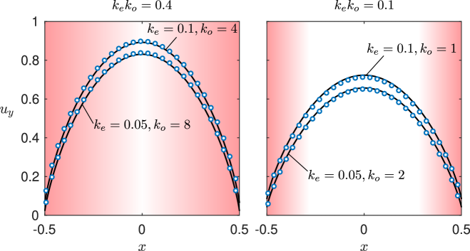
Figure 6: Velocity profiles in a vertical channel without disorder scattering ($G\to\infty$) and at zero magnetic field ($r_{c}^{-1}\to\infty$), with odd and even mean free paths chosen such that their product is constant at (a) $k_{e}k_{o}=0.4$ and (b) $k_{e}k_{o}=0.1$. Black lines show the analytical result (61), and blue open circles show a numerical solutions of the kinetic equation for comparison. The red shaded region indicates the approximate extent of the tomographic boundary layer, which is of order ${\it O}(\sqrt{k_{e}k_{o}})$.

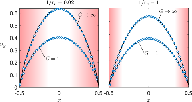
Figure 7: Velocity profile in a channel for weak and strong magnetic fields with (a) $r_{c}^{-1}=0.02$ and (b) $r_{c}^{-1}=1$, respectively, with $k_{e}=0.025$ and $k_{o}=5$. Each figure shows the velocity profile for weak disorder, $G=1$, and without any disorder scattering, $G\to\infty$. The extent of the tomographic boundary layer, which is indicated by the red shaded area, is suppressed with magnetic field.

We now discuss key features of the asymptotic solution to the velocity profile. At leading-order in $k_{e}$, the velocity profile in Eq. (61) is given by the widely-reported hydrodynamic $\cosh$ profile with no-slip boundary conditions (see Eq. (52)). At first order in $k_{e}$, however, the asymptotic solution strongly deviates from previous hydrodynamic solutions. In particular, at this order Eq. (61) exhibits (i) a significant velocity slip condition [the first line of Eq. (59)], which acts to increase the velocity profile; and (ii) tomographic bulk corrections [the second line of Eq. (59)], which act to decrease the velocity profile; (iii) tomographic boundary layer corrections [the $u_{T|y}^{(1)}$ term in Eq. (61)], which act to decrease the velocity profile. The approximate extent of the tomographic boundary layer, where the latter corrections are non-negligible, is shown in Figs. 6 and 7 with a red shaded region. In the absence of an external magnetic field, the tomographic boundary layer extends over the scaled distance $\sim\sqrt{k_{e}k_{o}}$; see Fig. 6. However, the width of the tomographic boundary layer is dramatically reduced in the presence of an external magnetic field; see Figs. 7. In particular, when the cyclotron radius is smaller than the odd-mode mean-free-path ($R_{c}<\ell_{o}$), the scaled tomographic boundary layer width scales instead as $\sim\sqrt{k_{e}r_{c}}$. Moreover, the magnitude of the velocity slip in the bulk solution, and the bulk finite-wavelength correction decreases significantly when an external magnetic field is applied. In particular, these decrease in magnitude as a Lorentzian with width $3\ell_{o}/R_{c}$. Together, these phenomena induce a negative magneto-conductance, which can be seen by comparing Fig. 7(a) and (b). Figure (7) shows that the width of the tomographic boundary layer is independent of the rate of bulk momentum-relaxation collisions. However, since the magnitude of the tomographic corrections is dictated by the boundary shear of the leading-order bulk flow and its normal derivative (see Eq. (17c)), the relative magnitude of the tomographic corrections increases with the frequency of bulk momentum relaxing collisions (i.e., increases when $G$ is decreased, see Eq. (61)). Similarly, the velocity slip of the bulk solution at ${\it O}(k_{e})$ (the third line of Eq. (61)) also increases with the frequency of bulk-momentum relaxing collisions.

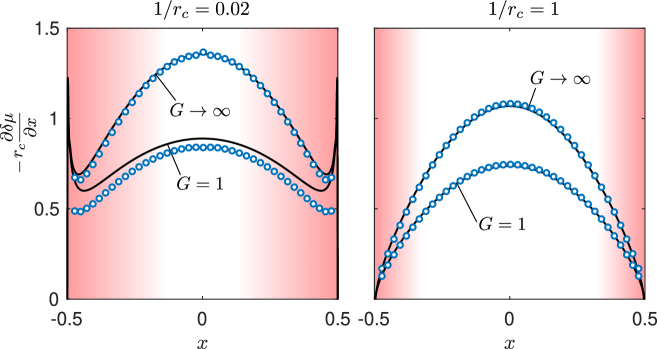
Figure 8: Same as Fig. 7 but for the rescaled Hall field, $-r_{c}\partial\delta\mu/\partial x$.

IV.2 Hall field

At leading order, the Hall field in the bulk is obtained by solving Eq. (15b),

$$-\frac{1}{2}\frac{\partial\delta\mu_{B}^{(0)}}{\partial x}-\frac{1}{r_{c}}u^{(0)}_{B|y} =0,$$ (62)

which gives

$$-\frac{\partial\delta\mu_{B}^{(0)}}{\partial x} =\frac{2}{r_{c}}u_{B|y}^{(0)}$$ (63)

with the leading-order bulk velocity profile reported in Eq. (52). With the same constraint equation, Eq. (53) implies

$$-\frac{\partial\delta\mu_{B}^{(1)}}{\partial x} =0.$$ (64)

Likewise, Eq. (15c) implies

$$-\frac{\partial\delta\mu_{B}^{(2)}}{\partial x} =\frac{2}{r_{c}}u_{B|y}^{(2)}.$$ (65)

with the higher-order velocity profile (59) that involves finite-wavelength corrections and slip-boundary conditions. On top of this, the bulk Hall field attains corrections in the tomographic boundary layer at $O(k_{e})$, which follows from the derivative of the third-order electrochemical potential $\delta\mu_{T}^{(3)}$ with respect to the rescaled boundary layer coordinate, Eq. (17),

$$-\sqrt{k_{e}}\frac{\partial\delta\mu_{T}^{(3)}}{\partial x}=\frac{2}{r_{c}}u_{T|y}^{(2)}$$

$$\hskip 50.00008pt-2\left[\mathcal{T}_{1}\left(\frac{\tfrac{1}{2}+x}{\sqrt{k_{e}k_{o}}};\frac{k_{o}}{r_{c}}\right)+\mathcal{T}_{1}\left(\frac{\tfrac{1}{2}-x}{\sqrt{k_{e}k_{o}}};\frac{k_{o}}{r_{c}}\right)\right]$$

$$-\frac{2G}{k_{o}}\tanh(\tfrac{1}{G})\left[\mathcal{T}_{0}\left(\frac{\tfrac{1}{2}+x}{\sqrt{k_{e}k_{o}}};\frac{k_{o}}{r_{c}}\right)+\mathcal{T}_{0}\left(\frac{\tfrac{1}{2}-x}{\sqrt{k_{e}k_{o}}};\frac{k_{o}}{r_{c}}\right)\right].$$ (66)

The factor $\sqrt{k_{e}}$ on the left-hand-side of Eq. (66) arises from the $O(\sqrt{k_{e}})$ width of the tomographic boundary layer. The full asymptotic solution for the Hall field up to ${\it O}(k_{e})$ thus reads

$$-\frac{\partial\delta\mu}{\partial x}= \frac{2}{r_{c}}u_{y}-k_{e}\Big{(}\sqrt{k_{e}}\frac{\partial\delta\mu_{T}^{(3)}}{\partial x}\Big{)}+{\it o}(k_{e}),$$ (67)

where $u_{y}$ is given in Eq. (61) and the second term in Eq. (66).

Figure 9: Microscopic Fermi surface deformation (solid black lines) for tomographic electron flow in a channel (a) for three different odd-parity mean free paths (top to bottom row) without magnetic field; and (b) for three different magnetic fields with fixed odd-parity mean free path. Shown are the deformation at different positions in the channel at $x=-0.5,-0.45,-0.3,0,0.3,0.45$, and $0.5$ (left to right columns), where the channel boundaries are at $x=\pm 0.5$. The dashed circles indicate the equilibrium Fermi surface. The diffuse boundary condition (12), where electrons impinging on the boundary are isotropically reflected, is directly apparent in the microscopic distribution at the boundary. In addition, all distributions have a center-of-mass displacement in the vertical direction, indicating electron flow in the positive $y$ direction. Without magnetic field, the electron density is fixed across the channel, corresponding to an unchanged area of the distribution. The area changes in the presence of a magnetic field, corresponding to the accumulation of charge at channel boundaries and the buildup of a Hall field. Parameters in (a) are $G\to\infty$ (no disorder), $r_{c}^{-1}=0$ (no magnetic field), $k_{e}=0.1$, and $k_{o}=0.25,1$, and $4$ (top to bottom rows). The distribution at the boundary is strongly non-uniform and decays by collisions to a hydrodynamic-like form (i.e., a deformation that predominantly involves a center-of-mass shift of the equilibrium distribution) in the channel center. The range over which this happens defines the tomographic boundary layer. The extent of this layer is ${\it O}(\sqrt{k_{e}k_{o}})$, and indeed it is apparent from panel (a) that it increases from the top to bottom row. Likewise, panel (b) shows the microscopic deformation with $G\to\infty$, $k_{e}=0.1$, and $k_{o}=5$ for three different magnetic fields $r_{c}^{-1}=0.02,0.1$, and $1$. While the tomographic layer extends to the channel center for weak field, it is quickly suppressed at stronger fields, where it only extends over a range ${\it O}(\sqrt{k_{e}r_{c}})$.

We now describe the asymptotic prediction for the Hall field in Eq. (67). In the bulk of the channel, the Hall field is given by the Lorentz force only up to $O(k_{e})$. No Hall viscosity contributions arise, being of ${\it O}(k_{e}^{2})$. The leading-order deviation of the Hall field from this classical description is thus given by the tomographic boundary layer functions, $\mathcal{T}_{0}$ and $\mathcal{T}_{1}$. Strikingly, these functions—and thus the Hall field near the boundaries—have a non-monotonic dependence on the magnetic field strength. This is demonstrated in Fig. 8, where the asymptotic solution for the Hall field is compared with direct numerical solutions of the linearized Boltzmann equation. This shows that the asymptotic theory overestimates the Hall field by up to 15% for the parameter values explored. Nonetheless, it correctly predicts the enhancement and divergence of the Hall field at the boundaries for a weak applied magnetic field, which is exhibited in the numerical solutions. As the magnetic field strength is increased, the Hall field qualitatively changes near the boundary, where it becomes suppressed; see Fig. 8. This is in strong contrast with the Hall field in conventional hydrodynamic flows, which is monotonic with the magnetic field strength [24, 25]. This new phenomenon gives a further point of distinction between the tomographic and hydrodynamic electron flow regimes.

IV.3 Fermi surface deformation

The full Fermi surface deformation $h$ is reconstructed directly from the solution of the velocity profile and the Hall field as discussed in Sec. II.4 and summarized in Tab. 2. Parameterizing the velocity in terms of the angle $\theta$ measured with respect to the positive $v_{x}$ axis [i.e., $v_{i}=(\cos\theta,\sin\theta)$ and $v_{i}^{\perp}=(\sin\theta,-\cos\theta)$], the bulk deformation reads

$$h_{B}^{(0)} =\delta\mu_{B}^{(0)}+2u^{(0)}_{B|y}\sin\theta,$$ (68)

$$h_{B}^{(2)} =\delta\mu_{B}^{(2)}+2u^{(2)}_{B|y}\sin\theta-\sin(2\theta)\frac{\partial u^{(0)}_{B|y}}{\partial x}$$

$$+\frac{1}{2}\frac{k_{o}}{1+(3k_{o}/r_{c})^{2}}\sin(3\theta)\frac{\partial^{2}u^{(0)}_{B|y}}{\partial x^{2}}$$

$$-\frac{3}{2}\frac{k_{o}^{2}/r_{c}}{1+(3k_{o}/r_{c})^{2}}\cos(3\theta)\frac{\partial^{2}u^{(0)}_{B|y}}{\partial x^{2}},$$ (69)

where $u^{(0)}_{B|y}$ and $u^{(2)}_{B|y}$ are listed in Eqs. (52) and (59), and $\delta\mu_{B}^{(0)}$ and $\delta\mu_{B}^{(2)}$ follow by integrating the Hall field in Eqs. (63) and (65). The structure of the bulk solution is directly apparent, with a hydrodynamic leading-order deformation $h_{B}^{(0)}$ that consist of a density and current deformation [the two terms in Eq. (68)], and a higher-order correction $h_{B}^{(2)}$ that in addition to density and current deformation [the first two terms in Eq. (69)] contains a shear deformation [third term] as well as an odd-parity tomographic ${\it O}(k_{o})$ correction [fourth and fifth terms]. The tomographic boundary layer correction (2), by contrast, contains all angular modes, and can be directly evaluated in terms of the general harmonic coefficients $a_{n}$ and $b_{n}$ of the boundary layer functions $f_{0}$ and $f_{1}$ reported in App. C.

We corroborate the above discussion by analyzing the Fermi surface deformation for flow in a channel. This deformation is shown in Fig. 9 and exhibits a strong dependence on the tomographic effect and the strength of the applied magnetic field. As $k_{o}$ is increased and in the absence of a magnetic field, the Fermi surface deformation exhibits a sharp feature for velocities parallel to the applied electric field (see Fig. 9(a)). The sharp feature in the Fermi surface deformation is most prominent near the device’s edges (i.e., in the tomographic boundary layer). When a magnetic field is applied, the sharp feature is suppressed as soon as $1/r_{c}\gtrsim k_{o}$ (see Fig. 9(b)). This is attributed to the magnetic-field both confining the tomographic boundary layer close to the boundary and suppressing the magnitude of tomographic phenomena, as was discussed previously.

V Summary and Outlook

In summary, we have derived an asymptotic theory describing steady two-dimensional tomographic electron flows in arbitrary geometries. The central result of our work are a set of flow equations for the electrochemical potential $\delta\mu$ and the velocity profile $u_{i}$, their boundary conditions and corrections in the tomographic boundary layer, which are summarized in Tab. 1. We also report the corresponding microscopic Fermi surface deformation, summarized in Tab. 2. These were obtained using a systematic asymptotic expansion of the underlying kinetic equation that includes multiple relaxation times, where the expansion parameter is the small ratio of the even-parity mean-free-path to the length scale of the flow (the even-mode Knudsen number $k_{e}$). The existence of such an expansion is a priori not obvious since the flow includes additional ballistic odd-mode degrees of freedom, and is thus markedly distinct from analogous expansions of the classical kinetic equation [22, 23] or conventional hydrodynamic theories with a single electronic relaxation time [24, 25].

Our framework has the dual advantage of offering analytical insight in tomographic flow effects as well as being very versatile, with existing solvers of conventional Stokes-Ohm equations being easily adaptable to solve the presented equations which embody the asymptotic theory for tomographic flows. In addition, the comparison between the predictions of our asymptotic theory for flow in a channel with exact numerical solutions of the kinetic equation shows excellent agreement even at non-negligible values of the expansion parameter $\sqrt{k_{e}}$, which suggests that our description can be used as an alternative to expensive numerical solutions of the kinetic equation. The theory reported here sets the foundations for future study of tomographic electron flows in other experimentally-relevant geometries, and it would be interesting to combine with numerical approaches to the Fermi-liquid equations [40, 41, 42]. This is of particular importance to geometries where hydrodynamic flows have been observed to exhibit novel phenomena, such as the superballistic conductance of flows through constrictions [43, 44, 8] and through a lattice of obstructions [40].

Appendix A Linearizing the electron Boltzmann equation

In this appendix, we summarize the linearization procedure of the Boltzmann equation for conduction electrons. This produces the linearized, scaled Boltzmann equation in Eq. (5). The starting point is the dimensional Boltzmann equation for the full distribution function $f$,

$$v_{i}\frac{\partial f}{\partial x_{i}}+e\left(\mathcal{E}_{i}-\frac{\partial\tilde{\Phi}}{\partial x_{i}}+\varepsilon_{ijk}v_{i}\mathcal{B}_{j}\right)\frac{\partial f}{\partial v_{k}}=$$

$$-\frac{1}{\tau_{e}}\left[f-f_{\text{MC}}\right]_{e}-\frac{1}{\tau_{o}}\left[f-f_{\text{MC}}\right]_{o}+\frac{1}{\tau_{\text{MR}}}\left(f-f_{\text{MR}}\right),$$ (70)

where $x_{i}$ and $v_{i}$ are (dimensional) position and velocity coordinates, $\tilde{\Phi}$ is the dimensional induced electric potential, and ${\cal B}_{i}$ and ${\cal E}_{i}$ the external (dimensional) magnetic and electric fields. The left-hand side of Eq. (70) is the streaming term and the right-hand side is the collision term. For the latter, we adopt a generalized relaxation-time approximation that accounts for momentum-conserving collisions with constant relaxation times $\tau_{e}$ and $\tau_{o}$ for the distribution function’s even and odd modes as well as residual momentum relaxing collisions with a relaxation time $\tau_{\text{MR}}$. These relaxation times are related to the respective collisional mean free paths via $\ell_{\alpha}=v_{F}\tau_{\alpha}$ (with $\alpha=e,o,\text{MR}$). The momentum-conserving and momentum-relaxing collisions are assumed to relax the distribution function to a local moving and stationary equilibrium, respectively,

$$f_{\text{MC}}= \left[1+\exp\left(\frac{\frac{1}{2}m^{*}(v_{i}-\bar{v}_{i})^{2}-\mu}{k_{B}T}\right)\right]^{-1},$$ (71a)

$$f_{\text{MR}}= \left[1+\exp\left(\frac{\frac{1}{2}m^{*}v_{i}^{2}-\mu}{k_{B}T}\right)\right]^{-1},$$ (71b)

where $T$ is the local temperature, $\mu$ is the local chemical potential, $\bar{v}_{i}$ is the local drift velocity. We assume a parabolic dispersion relation throughout. In the following, we will expand Eq. (70) for low temperatures relative to the Fermi temperature and for weak driving electric fields, where the form of the collision operator on the right-hand side of Eq. (70) is applicable.

To linearize Eq. (70), we first scale the velocity and spatial coordinates by $v_{F}$ and $L$, respectively. The applied electric and magnetic fields are scaled by their respective magnitudes $\mathcal{E}$ and $\mathcal{B}$, and the induced electric potential by $\mathcal{E}L$,

$$\mathcal{E}_{i}=\mathcal{E}E_{i},\qquad\mathcal{B}_{i}=\mathcal{B}B_{i},\qquad\tilde{\Phi}=\mathcal{E}L\Phi.$$ (72)

We then introduce the electron Mach number,

$$\text{Ma}=\frac{U}{v_{F}},$$ (73)

where $U=e\mathcal{E}L^{2}/(m^{*}v_{F}^{2}\tau_{e})$ is the hydrodynamic velocity scale. The Boltzmann equation is linearized by expanding the distribution function and each of the macroscopic variables for small Mach number, followed by an expansion of small temperature relative to the Fermi temperature,

$$\text{Ma}\ll 1,\qquad\frac{T}{T_{F}}\ll 1.$$ (74)

The former expansion is applicable for weak driving electric fields, and the latter is applicable to degenerate systems and confines all excitations to the Fermi surface, which is assumed isotropic. The expansion for the distribution function and electrochemical potential then reads

$$f =f_{0}+\text{Ma}\,E_{F}\biggl{(}-\frac{\partial f_{0}}{\partial E}\biggr{)}\left(h+2k_{e}\Phi\right)$$

$$\qquad+{\it O}\biggl{(}\text{Ma}^{2},\biggr{(}\frac{T}{T_{F}}\biggr{)}^{2}\biggr{)},$$ (75a)

$$\mu =E_{F}\biggl{[}1+\text{Ma}\left(\delta\mu+2k_{e}\Phi\right)+{\it O}\biggl{(}\text{Ma}^{2},\biggr{(}\frac{T}{T_{F}}\biggr{)}^{2}\biggr{)}\biggr{]},$$ (75b)

where $f_{0}$ is the global equilibrium distribution, $E=m^{*}v^{2}/2$ is the energy of the electrons, and $E_{F}=m^{*}v_{F}^{2}/2$ the Fermi energy. Furthermore, $h$ and $\delta\mu$ are the scaled linear perturbations of the distribution function and electrochemical potential, respectively. The dimensionless bulk velocity, $u_{i}$, is defined via $\bar{v}_{i}=v_{F}\text{Ma}\,u_{i}$, which follows directly from the definition of the Mach number in Eq. (73). The macroscopic variables $\delta\mu$ and $u_{i}$ are given by the zeroth and first moment of the distribution function as reported in the main text (Eqs. (6) and (7)). Substituting the expansion (75) into Eqs. (70) and (71) and collecting terms linear in Ma gives the linearized Boltzmann equation (5) reported in the main text.

Appendix B Coordinate form of stress tensor derivatives

This appendix collects some derivative identities that are used to obtain the coordinate representation of the boundary condition (46). Similar identities have been reported in the classical gas literature, see, for example, Refs. [45, 46, 28]. First, to express the higher-moment even-parity correction in coordinate form, we note

$$\biggl{[}t_{i}t_{j}\frac{\partial u_{B|i}^{(0)}}{\partial x_{j}}\biggr{]}_{S} =0,$$ (76)

$$\biggl{[}n_{i}n_{j}\frac{\partial u_{B|i}^{(0)}}{\partial x_{j}}\biggr{]}_{S} =0.$$ (77)

The first identity follows from the no-slip boundary condition $t_{i}u_{B|i}^{(0)}=0$, which holds identically along the boundary, and the second one follows from the continuity equation and the no-slip condition. Since these equations hold identically along the boundary, they imply the additional identities

$$t_{k}\frac{\partial}{\partial x_{k}}\biggl{(}t_{i}t_{j}\frac{u_{B|i}^{(0)}}{\partial x_{j}}\biggr{)} =0,$$ (78)

$$t_{k}\frac{\partial}{\partial x_{k}}\biggl{(}n_{i}n_{j}\frac{u_{B|i}^{(0)}}{\partial x_{j}}\biggr{)} =0.$$ (79)

To rewrite the higher-order odd-parity contributions, we need the additional identity

$$\biggl{[}n_{i}t_{j}t_{k}\frac{\partial^{2}u_{B|i}^{(0)}}{\partial x_{j}\partial x_{k}}\biggr{]}_{S} =0,$$ (80)

which follows from the no-penetration boundary condition that again holds identically along the boundary. In addition, we have

$$\biggl{[}n_{i}n_{j}n_{k}\frac{\partial^{2}u_{B|i}^{(0)}}{\partial x_{j}x_{k}}\biggr{]}_{S} =-\frac{1}{2}n_{i}n_{j}\biggl{[}n_{k}\frac{\partial S_{B|ij}^{(0)}}{\partial x_{k}}\biggr{]}_{S},$$ (81)

where the rate-of-strain tensor is defined in Eq. (19). Furthermore,

$$\biggl{[}n_{i}t_{j}n_{k}\frac{\partial^{2}u_{B|i}^{(0)}}{\partial x_{j}\partial x_{k}}\biggr{]}_{S} =\kappa\,\Bigl{[}n_{i}t_{j}S_{B|ij}^{(0)}\Bigr{]}_{S}.$$ (82)

We use this relation to obtain the following identity

$$\biggl{[}t_{i}n_{j}n_{k}\frac{\partial^{2}u_{B|i}^{(0)}}{\partial x_{j}\partial x_{k}}\biggr{]}_{S}$$

$$\quad=\biggl{[}-t_{i}n_{j}n_{k}\frac{\partial S_{B|ij}^{(0)}}{\partial x_{k}}\biggr{]}_{S}-\kappa\,\Bigl{[}n_{i}t_{j}S_{B|ij}^{(0)}\Bigr{]}_{S}.$$ (83)

In addition, using the incompressibility condition gives

$$\biggl{[}t_{i}n_{j}t_{k}\frac{\partial^{2}u_{B|i}^{(0)}}{\partial x_{j}\partial x_{k}}\biggr{]}_{S} =\frac{1}{2}\biggl{[}n_{i}n_{j}n_{k}\frac{\partial S_{B|ij}^{(0)}}{\partial x_{k}}\biggr{]}_{S}.$$ (84)

Finally,

$$\biggl{[}t_{i}t_{j}t_{k}\frac{\partial^{2}u_{B|i}^{(0)}}{\partial x_{j}\partial x_{k}}\biggr{]}_{S} =-\kappa\,\Bigl{[}n_{i}t_{j}S_{B|ij}^{(0)}\Bigr{]}_{S}.$$ (85)

We also need the Laplace identities

$$\biggl{[}n_{i}\frac{\partial^{2}u_{B|i}^{(0)}}{\partial x_{j}^{2}}\biggr{]}_{S} =-\frac{1}{2}\biggl{[}n_{i}n_{j}n_{k}\frac{\partial S_{B|ij}^{(0)}}{\partial x_{k}}\biggr{]}_{S},$$ (86)

$$\biggl{[}t_{i}\frac{\partial^{2}u_{B|i}^{(0)}}{\partial x_{j}^{2}}\biggr{]}_{S} =-2\kappa\,\Bigl{[}n_{i}t_{j}S_{B|ij}^{(0)}\Bigr{]}_{S}-\biggl{[}t_{i}n_{j}n_{k}\frac{\partial S_{B|ij}^{(0)}}{\partial x_{k}}\biggr{]}_{S},$$ (87)

where we used Eqs. (81) and (80) for the first identity and Eqs. (83) and (85) for the second identity.

Taken together, we obtain the coordinate representation

$$\biggl{[}v_{i}v_{j}\frac{\partial u_{H,j}^{(0)}}{\partial x_{i}}\biggr{]}_{S}=-\sin 2\theta\,\Bigl{[}n_{i}t_{j}S_{B|ij}^{(0)}\Bigr{]}_{S}$$ (88)

$$\biggl{[}v_{i}v_{j}v_{k}-\frac{1}{4}\delta_{ik}v_{j}\biggr{]}\biggl{[}\frac{\partial^{2}u_{H,j}^{(0)}}{\partial x_{i}\partial x_{k}}\biggr{]}_{S}$$

$$=-\frac{\kappa}{2}\cos(3\theta)\,\Bigl{[}n_{i}t_{j}S_{B|ij}^{(0)}\Bigr{]}_{S}+\frac{\cos(3\theta)}{4}\,\biggl{[}t_{i}n_{j}n_{k}\frac{\partial S_{B|ij}^{(0)}}{\partial x_{k}}\biggr{]}_{S}$$

$$\quad+\frac{3}{8}\sin(3\theta)\,\biggl{[}n_{i}n_{j}n_{k}\frac{\partial S_{B|ij}^{(0)}}{\partial x_{k}}\biggr{]}_{S}$$ (89)

$$\biggl{[}v_{i}^{\perp}v_{j}^{\perp}v_{k}^{\perp}-\frac{1}{4}\delta_{ik}v_{j}^{\perp}\biggr{]}\biggl{[}\frac{\partial^{2}u_{H,j}^{(0)}}{\partial x_{i}\partial x_{k}}\biggr{]}_{S}$$

$$=\frac{\kappa}{2}\sin(3\theta)\,\Bigl{[}n_{i}t_{j}S_{B|ij}^{(0)}\Bigr{]}_{S}-\frac{1}{4}\sin(3\theta)\,\biggl{[}t_{i}n_{j}n_{k}\frac{\partial S_{B|ij}^{(0)}}{\partial x_{k}}\biggr{]}_{S}$$

$$\quad+\frac{3}{8}\cos(3\theta)\,\biggl{[}n_{i}n_{j}n_{k}\frac{\partial S_{B|ij}^{(0)}}{\partial x_{k}}\biggr{]}_{S}.$$ (90)

Appendix C Truncated moment expansion solution of the tomographic boundary layer corrections

This appendix presents an efficient numerical solution to Eq. (2), which describes the tomographic boundary layer, using a truncated moment expansion. Substituting Eq. (2)—which expresses the tomographic boundary deformation $h_{T}^{(2)}$ in terms of three scalar boundary layer functions $f_{0},f_{1}$ and $f_{2}$—into the tomographic Eq. (2), we obtain the governing equations for each set of $f_{i}$, $\mathcal{Y}_{i}$ and $\mathcal{T}_{i}$ (the latter are defined in Eqs. (17c) and (17)),

$$\sin^{2}\theta\frac{\partial^{2}f_{i}}{\partial\chi^{2}}-f_{i}-\frac{k_{o}}{r_{c}}\frac{\partial f_{i}}{\partial\theta}$$

$$\quad=-2\cos\theta\mathcal{Y}_{i}+\sin\theta\biggl{(}\mathcal{T}_{i}+\frac{2k_{o}}{r_{c}}\mathcal{Y}_{i}\biggr{)}$$ (91)

with $i\in\{0,1,2\}$. The boundary condition for $h_{T}^{(2)}$ in Eq. (46) gives the following condition for each $f_{i}$ at $\chi=0$,

$$\bigl{[}f_{0}\bigr{]}_{S}= \frac{64}{15\pi}\cos\theta-\sin(2|\theta|),$$ (92a)

$$\bigl{[}f_{1}\bigr{]}_{S}= \frac{\cos\theta+\cos(3\theta)+3k_{o}/r_{c}\sin(3\theta)}{1+(3k_{o}/r_{c})^{2}},$$ (92b)

$$\bigl{[}f_{2}\bigr{]}_{S}= \frac{3}{4}\frac{3k_{o}/r_{c}(\cos\theta+\cos(3\theta))-\sin(3\theta)}{1+(3k_{o}/r_{c})^{2}}.$$ (92c)

We solve these equations using a truncated moment expansion: Each of the distribution functions is expanded in the truncated series,

$$f_{i}(\chi,\theta)=\sum_{n\,{\rm odd}}^{N}\bigl{[}a_{n}(\chi)\cos(n\theta)+b_{n}(\chi)\sin(n\theta)\bigr{]},$$ (93)

for each of $i=0,1,2$, where $a_{n}$ and $b_{n}$ are functions of $\chi$ and $k_{o}/r_{c}$, and $N$ is an integer that sets the cutoff of the expansion. Only odd $n\geq 1$ contribute to this expansion since the tomographic boundary layer functions all have odd parity [cf. Eq. (39)]. Note that the no-penetration boundary condition implies $b_{1}=0$ and Eq. (48) implies $a_{1}=a_{3}$. Substituting Eq. (93) into Eq. (91) and then projecting Eq. (91) onto the subspace spanned by the basis functions of Eq. (93) gives a system of coupled ordinary differential equations for $a_{n}$ and $b_{n}$,

$$\begin{pmatrix}A_{N}&0\\[4.30554pt] 0&B_{N}\end{pmatrix}\begin{pmatrix}\bf{a}\\[4.30554pt] \bf{b}\end{pmatrix}^{\prime\prime}=\begin{pmatrix}I_{N}&\frac{k_{o}}{r_{c}}C_{N}\\[4.30554pt] -\frac{k_{o}}{r_{c}}C_{N}&I_{N}\end{pmatrix}\begin{pmatrix}\bf{a}\\[4.30554pt] \bf{b}\end{pmatrix}.$$ (94)

Here, $\mathbf{a}=(a_{3},\dots,a_{N})^{T},\mathbf{b}=(b_{3},\dots,b_{N})^{T}$, $I_{N}$ is the $N\times N$ identity matrix, the prime symbol is used to denote differentiation with respect to $\chi$, $C_{N}$ is a diagonal matrix with entries $[C_{N}]_{kk^{\prime}}=(2k+1)\delta_{kk^{\prime}}$, and we define

$$A_{N}= \begin{pmatrix}\frac{1}{4}&-\frac{1}{4}&0&0&\cdots&0\\[4.30554pt] -\frac{1}{4}&\frac{1}{2}&-\frac{1}{4}&0&\cdots&0\\[4.30554pt] 0&-\frac{1}{4}&\frac{1}{2}&-\frac{1}{4}&\cdots&0\\[4.30554pt] \vdots&&&\ddots&&\vdots\\[4.30554pt] 0&0&0&-\frac{1}{4}&\frac{1}{2}&-\frac{1}{4}\\[4.30554pt] 0&0&0&0&-\frac{1}{4}&\frac{1}{2}\end{pmatrix},$$ (95a)

$$B_{N}= \begin{pmatrix}\frac{1}{2}&-\frac{1}{4}&0&0&\cdots&0\\[4.30554pt] -\frac{1}{4}&\frac{1}{2}&-\frac{1}{4}&0&\cdots&0\\[4.30554pt] 0&-\frac{1}{4}&\frac{1}{2}&-\frac{1}{4}&\cdots&0\\[4.30554pt] \vdots&&&\ddots&&\vdots\\[4.30554pt] 0&0&0&-\frac{1}{4}&\frac{1}{2}&-\frac{1}{4}\\[4.30554pt] 0&0&0&0&-\frac{1}{4}&\frac{1}{2}\end{pmatrix}.$$ (95b)

Equation (94) is then solved numerically for each fixed value of $k_{o}/r_{c}$ by expanding in eigenvectors

$$\begin{pmatrix}\bf{a}\\[4.30554pt] \bf{b}\end{pmatrix}=\sum_{j}c_{j}{\bf v}_{j}\exp\Bigl{(}-\sqrt{\lambda_{j}}\,\chi\Bigr{)},$$ (96)

where ${\bf v}_{j}$ and $\lambda_{j}$ are the eigenvectors and eigenvalues of the matrix

$$M_{N}=\begin{pmatrix}A_{N}&0\\[4.30554pt] 0&B_{N}\end{pmatrix}^{-1}\begin{pmatrix}I_{N}&(k_{o}/r_{c})C_{N}\\[4.30554pt] -(k_{o}/r_{c})C_{N}&I_{N}\end{pmatrix},$$ (97)

which are evaluated numerically. The coefficients $c_{i}$ in Eq. (96) are then found by projecting the boundary conditions in Eq. (92) onto the basis functions of Eq. (93), which gives boundary conditions for $\bf{a}$ and $\bf{b}$ at $\chi=0$. They are, for $f_{0}$,

$$[a_{n}]_{S} =\dfrac{8}{\pi(n+2)(n-2)},$$ (98)

$$[b_{n}]_{S} =0,$$ (99)

and for $f_{1}$,

$$[a_{n}]_{S} =\begin{cases}\dfrac{1}{1+(3k_{o}/r_{c})^{2}}&n=3\\[4.30554pt] 0&{\rm otherwise}\end{cases},$$ (100)

$$[b_{n}]_{S} =\begin{cases}\dfrac{3k_{o}/r_{c}}{1+(3k_{o}/r_{c})^{2}}&n=3\\[4.30554pt] 0&{\rm otherwise}\end{cases},$$ (101)

and for $f_{2}$,

$$[a_{n}]_{S} =\begin{cases}\dfrac{9}{4}\dfrac{k_{o}/r_{c}}{1+(3k_{o}/r_{c})^{2}}&n=3\\[6.45831pt] 0&{\rm otherwise}\end{cases},$$ (102)

$$[b_{n}]_{S} =\begin{cases}-\dfrac{3}{4}\dfrac{1}{1+(3k_{o}/r_{c})^{2}}&n=3\\[4.30554pt] 0&{\rm otherwise}\end{cases}.$$ (103)

The value of $N$ is increased until convergence is obtained. A final value of $N=100$ was used in generating the plots of the tomographic boundary layer functions in Fig. 4. The solution for ${\cal Y}_{i}$ and ${\cal T}_{i}$ is then obtained using

$${\cal Y}_{i} =\frac{a_{1}}{2}=\frac{a_{3}}{2}.$$ (104)

$${\cal T}_{i} =-\frac{1}{4}\frac{d^{2}b_{3}}{d\chi^{2}}.$$ (105)

Appendix D Numerical solution for channel flow

This appendix summarizes the numerical solutions to Eq. (5) for flow in a channel, which we use in the main text to compare with the result of the asymptotic expansion. Further details are described in [25]. Equation (5) is discretized with $N_{x}$ and $N_{\theta}$ points in the spatial and velocity coordinate, respectively, where the spatial points are concentrated near the boundaries $x=\pm 1/2$. Derivatives are then approximated at each mesh point using a finite volume method, and moments of the distribution function are approximated using the trapezoidal rule. A time derivative is added to the left hand side of Eq. (5) which is discretized using the second-order Runge-Kutta method and iterated from global equilibrium until a steady state is achieved. The number of spatial and velocity points is then increased until the solution changes by less than 1% with further mesh refinements. A final mesh of $N_{x}=300$ and $N_{\theta}=200$ is used.

References

- Fritz and Scaffidi [2024] L. Fritz and T. Scaffidi, Hydrodynamic Electronic Transport, Annual Review of Condensed Matter Physics 15, 17 (2024).
- Varnavides et al. [2023] G. Varnavides, A. Yacoby, C. Felser, and P. Narang, Charge transport and hydrodynamics in materials, Nature Reviews Materials 8, 726 (2023).
- Forster [1990] D. Forster, Hydrodynamics Fluctuations, Broken Symmetry, and Correlation Functions (Perseus Books, New York, 1990).
- Aharon-Steinberg et al. [2022] A. Aharon-Steinberg, T. Völkl, A. Kaplan, A. K. Pariari, I. Roy, T. Holder, Y. Wolf, A. Y. Meltzer, Y. Myasoedov, M. E. Huber, B. Yan, G. Falkovich, L. S. Levitov, M. Hücker, and E. Zeldov, Direct observation of vortices in an electron fluid, Nature 607, 74 (2022).
- Sulpizio et al. [2019] J. A. Sulpizio, L. Ella, A. Rozen, J. Birkbeck, D. J. Perello, D. Dutta, M. Ben-Shalom, T. Taniguchi, K. Watanabe, T. Holder, R. Queiroz, A. Principi, A. Stern, T. Scaffidi, A. K. Geim, and S. Ilani, Visualizing Poiseuille flow of hydrodynamic electrons, Nature 576, 75 (2019).
- Ku et al. [2020] M. J. H. Ku, T. X. Zhou, Q. Li, Y. J. Shin, J. K. Shi, C. Burch, L. E. Anderson, A. T. Pierce, Y. Xie, A. Hamo, U. Vool, H. Zhang, F. Casola, T. Taniguchi, K. Watanabe, M. M. Fogler, P. Kim, A. Yacoby, and R. L. Walsworth, Imaging viscous flow of the Dirac fluid in graphene, Nature 583, 537 (2020).
- Vool et al. [2021] U. Vool, A. Hamo, G. Varnavides, Y. Wang, T. X. Zhou, N. Kumar, Y. Dovzhenko, Z. Qiu, C. A. C. Garcia, A. T. Pierce, J. Gooth, P. Anikeeva, C. Felser, P. Narang, and A. Yacoby, Imaging phonon-mediated hydrodynamic flow in WTe2, Nature Physics 17, 1216 (2021).
- Krebs et al. [2023] Z. J. Krebs, W. A. Behn, S. Li, K. J. Smith, K. Watanabe, T. Taniguchi, A. Levchenko, and V. W. Brar, Imaging the breaking of electrostatic dams in graphene for ballistic and viscous fluids, Science 379, 671 (2023).
- Kiselev and Schmalian [2019] E. I. Kiselev and J. Schmalian, Boundary conditions of viscous electron flow, Phys. Rev. B 99, 035430 (2019).
- Moessner et al. [2019] R. Moessner, N. Morales-Durán, P. Surówka, and P. Witkowski, Boundary-condition and geometry engineering in electronic hydrodynamics, Phys. Rev. B 100, 155115 (2019).
- De Jong and Molenkamp [1995] M. J. M. De Jong and L. W. Molenkamp, Hydrodynamic Electron Flow in High-Mobility Wires, Physical Review B 51, 13389 (1995).
- Knudsen [1909] M. Knudsen, Die Gesetze der Molekularströmung und der inneren Reibungsströmung der Gase durch Röhren, Annalen der Physik 333, 75 (1909).
- Baker et al. [2024] G. Baker, M. Moravec, and A. P. Mackenzie, A Perspective on Non-Local Electronic Transport in Metals: Viscous, Ballistic, and Beyond, Annalen der Physik 2024, 2400087 (2024).
- Laikhtman [1992] B. Laikhtman, Electron-Electron Angular Relaxation in a Two-Dimensional Electron Gas, Physical Review B 45, 1259 (1992).
- Nilsson and Castro Neto [2005] J. Nilsson and A. H. Castro Neto, Heat bath approach to Landau damping and Pomeranchuk quantum critical points, Phys. Rev. B 72, 195104 (2005).
- Gurzhi et al. [1995] R. N. Gurzhi, A. N. Kalinenko, and A. I. Kopeliovich, Electron-Electron Collisions and a New Hydrodynamic Effect in Two-Dimensional Electron Gas, Phys. Rev. Lett. 74, 3872 (1995).
- Ledwith et al. [2019] P. Ledwith, H. Guo, A. Shytov, and L. Levitov, Tomographic Dynamics and Scale-Dependent Viscosity in 2D Electron Systems, Phys. Rev. Lett. 123, 116601 (2019).
- Ledwith et al. [2017] P. Ledwith, H. Guo, and L. Levitov, Angular superdiffusion and directional memory in two-dimensional electron fluids, arXiv preprint arXiv:1708.01915 10.48550/arXiv.1708.01915 (2017).
- Hofmann and Gran [2023] J. Hofmann and U. Gran, Anomalously long lifetimes in two-dimensional Fermi liquids, Phys. Rev. B 108, L121401 (2023).
- Nilsson et al. [2024] E. Nilsson, U. Gran, and J. Hofmann, Nonequilibrium relaxation and odd-even effect in finite-temperature electron gases, arXiv preprint arXiv:2405.03635 10.48550/arXiv.2405.03635 (2024).
- Nazaryan and Levitov [2024] K. G. Nazaryan and L. Levitov, Nonlocal conductivity, continued fractions, and current vortices in electron fluids, Phys. Rev. B 110, 045147 (2024).
- Sone [2002] Y. Sone, Kinetic Theory and Fluid Dynamics (Birkhäuser Boston, 2002).
- Sone [2007] Y. Sone, Molecular gas dynamics: theory, techniques, and applications (Springer, 2007).
- Ben-Shachar et al. [2025a] N. Ben-Shachar, J. T. Johnson, M. Madadi, J. Nassios, and J. E. Sader, Hall field and odd viscosity in near-hydrodynamic electron flows, Phys. Rev. B Letters (accepted) (2025a).
- Ben-Shachar et al. [2025b] N. Ben-Shachar, J. T. Johnson, M. Madadi, J. Nassios, and J. E. Sader, Near-hydrodynamic electron flow according to the linearized Boltzmann equation, Phys. Rev. B (accepted) (2025b).
- Hofmann and Das Sarma [2022] J. Hofmann and S. Das Sarma, Collective modes in interacting two-dimensional tomographic Fermi liquids, Phys. Rev. B 106, 205412 (2022).
- Ben-Shachar and Hofmann [2025] N. Ben-Shachar and J. Hofmann, Magnetotransport of tomographic electrons in a channel (2025).
- Nassios and Sader [2012] J. Nassios and J. E. Sader, Asymptotic analysis of the Boltzmann–BGK equation for oscillatory flows, Journal of Fluid Mechanics 708, 197–249 (2012).
- Alekseev [2016] P. S. Alekseev, Negative Magnetoresistance in Viscous Flow of Two-Dimensional Electrons, Phys. Rev. Lett. 117, 166601 (2016).
- Scaffidi et al. [2017] T. Scaffidi, N. Nandi, B. Schmidt, A. P. Mackenzie, and J. E. Moore, Hydrodynamic Electron Flow and Hall Viscosity, Phys. Rev. Lett. 118, 226601 (2017).
- Matthaiakakis et al. [2020] I. Matthaiakakis, D. Rodríguez Fernández, C. Tutschku, E. M. Hankiewicz, J. Erdmenger, and R. Meyer, Functional dependence of Hall viscosity induced transverse voltage in two-dimensional Fermi liquids, Phys. Rev. B 101, 045423 (2020).
- Afanasiev et al. [2022] A. N. Afanasiev, P. S. Alekseev, A. A. Danilenko, A. P. Dmitriev, A. A. Greshnov, and M. A. Semina, Hall effect in Poiseuille flow of two-dimensional electron fluid, Phys. Rev. B 106, 245415 (2022).
- Palm et al. [2024] M. L. Palm, C. Ding, W. S. Huxter, T. Taniguchi, K. Watanabe, and C. L. Degen, Observation of current whirlpools in graphene at room temperature, Science 384, 465 (2024).
- Pellegrino et al. [2016] F. M. D. Pellegrino, I. Torre, A. K. Geim, and M. Polini, Electron hydrodynamics dilemma: Whirlpools or no whirlpools, Phys. Rev. B 94, 155414 (2016).
- Raichev [2022] O. E. Raichev, Linking boundary conditions for kinetic and hydrodynamic description of fermion gas, Phys. Rev. B 105, L041301 (2022).
- Gran et al. [2023] U. Gran, E. Nilsson, and J. Hofmann, Shear viscosity in interacting two-dimensional Fermi liquids, arXiv preprint arXiv:2312.09977 10.48550/arXiv.2312.09977 (2023).
- Lucas [2017] A. Lucas, Stokes paradox in electronic Fermi liquids, Phys. Rev. B 95, 115425 (2017).
- Liu et al. [2020] N. Z. Liu, D. R. Ladiges, J. Nassios, and J. E. Sader, Acoustic flows in a slightly rarefied gas, Phys. Rev. Fluids 5, 043401 (2020).
- Holder et al. [2019] T. Holder, R. Queiroz, T. Scaffidi, N. Silberstein, A. Rozen, J. A. Sulpizio, L. Ella, S. Ilani, and A. Stern, Ballistic and hydrodynamic magnetotransport in narrow channels, Phys. Rev. B 100, 245305 (2019).
- Estrada-Álvarez et al. [2024a] J. Estrada-Álvarez, J. Salvador-Sánchez, A. Pérez-Rodríguez, C. Sánchez-Sánchez, V. Clericò, D. Vaquero, K. Watanabe, T. Taniguchi, E. Diez, F. Domínguez-Adame, et al., Superballistic conduction in hydrodynamic antidot graphene superlattices, arXiv preprint arXiv:2407.04527 10.48550/arXiv.2407.04527 (2024a).
- Estrada-Álvarez et al. [2024b] J. Estrada-Álvarez, F. Domínguez-Adame, and E. Díaz, Alternative routes to electron hydrodynamics, Communications Physics 7, 138 (2024b).
- Estrada-Álvarez et al. [2025] J. Estrada-Álvarez, E. Díaz, and F. Domínguez-Adame, Superballistic paradox in electron fluids: Evidence of tomographic transport (2025), arXiv:2502.10265 [cond-mat.mes-hall] .
- Krishna Kumar et al. [2017] R. Krishna Kumar, D. A. Bandurin, F. M. D. Pellegrino, Y. Cao, A. Principi, H. Guo, G. H. Auton, M. Ben Shalom, L. A. Ponomarenko, G. Falkovich, K. Watanabe, T. Taniguchi, I. V. Grigorieva, L. S. Levitov, M. Polini, and A. K. Geim, Superballistic flow of viscous electron fluid through graphene constrictions, Nature Physics 13, 1182 (2017).
- Stern et al. [2022] A. Stern, T. Scaffidi, O. Reuven, C. Kumar, J. Birkbeck, and S. Ilani, How Electron Hydrodynamics Can Eliminate the Landauer-Sharvin Resistance, Phys. Rev. Lett. 129, 157701 (2022).
- Sone [1969] Y. Sone, Asymptotic theory of flow of rarefied gas over a smooth boundary I, in Rarefied Gas Dynamics, edited by L. Trilling and H. Y. Wachman (Academic Press, 1969) pp. 243–253.
- Sone [1971] Y. Sone, Asymptotic theory of flow of rarefied gas over a smooth boundary II, in Rarefied Gas Dynamics, edited by D. Dini (Editrice Tecnico Scientifica, Pisa, 1971) p. 737.