Doubly robust identification of treatment effects
from multiple environments

Abstract

Practical and ethical constraints often require the use of observational data for causal inference, particularly in medicine and social sciences. Yet, observational datasets are prone to confounding, potentially compromising the validity of causal conclusions. While it is possible to correct for biases if the underlying causal graph is known, this is rarely a feasible ask in practical scenarios. A common strategy is to adjust for all available covariates, yet this approach can yield biased treatment effect estimates, especially when post-treatment or unobserved variables are present. We propose Ramen, an algorithm that produces unbiased treatment effect estimates by leveraging the heterogeneity of multiple data sources without the need to know or learn the underlying causal graph. Notably, Ramen achieves doubly robust identification: it can identify the treatment effect whenever the causal parents of the treatment or those of the outcome are observed, and the node whose parents are observed satisfies an invariance assumption. Empirical evaluations on synthetic and real-world datasets show that our approach outperforms existing methods.

1 Introduction

Treatment effects are key quantities of interest in applied domains such as medicine and social sciences, as they determine the impact of interventions like novel treatments or policies on outcomes of interest. To achieve this goal, researchers often rely on randomized trials since randomizing the treatment assignment guarantees unbiased treatment effect estimates under mild assumptions. However, methods relying on randomized data face several issues, such as small sample sizes, sample populations that do not reflect those seen in the real world, and ethical or financial constraints. As a result, there is growing interest in using observational data to estimate treatment effects.

A fundamental challenge in using observational data is the selection of a valid adjustment set, i.e. a set of covariates that can be used to identify and estimate the treatment effect. Although criteria for identifying valid adjustment sets are well-established, they rely on the knowledge of the underlying causal graph. When the graph is not known, practitioners often adjust for all available covariates [5]. Yet, this approach runs the risk of including bad controls—covariates that open backdoor paths between the treatment ($T$) and the outcome ($Y$), thereby introducing bias into the treatment effect estimate. For instance, consider the causal graphs illustrated in Figure 1, where $\{X_{1},X_{2}\}$ are the observed covariates. In Figure 1(a), both $X_{1}$ and $X_{2}$ are parents of $T$, and adjusting for $\{X_{1},X_{2}\}$ blocks all backdoor paths between $T$ and $Y$, making it a valid adjustment set. In contrast, in Figure 1(b), $X_{1}$ is a child of $T$, and conditioning on it opens a backdoor path between $T$ and $Y$, introducing bias in the effect estimate. In the latter case, $X_{1}$ is referred to as a bad control.

Bad controls pose a significant challenge when the causal ordering of the observed covariates is not clear [47, 55]. A prominent example for a bad control is the birth-weight paradox [90] from which it was concluded that when estimating the effect of maternal smoking ($T$) on infant mortality ($Y$), the birth weight would be a bad control like $X_{1}$ in Figure 1(b), as it is a child node of $T$ and likely leads to collider bias. Further, Acharya et al. [1] found that up to two-thirds of empirical studies in political science that make causal claims inadvertently include bad controls in their analysis, leading to biased treatment effect estimates. Several works have tried to tackle the problem of bad controls using expert-driven structural knowledge, e.g. by leveraging anchor variables [10, 75], but such domain expertise is often unavailable in practice. Shi et al. [79] propose an alternative approach that leverages access to multiple heterogeneous data sources—e.g. observational studies from different countries—to identify and estimate the treatment effect in the presence of bad controls. Yet, their approach can fail to identify the treatment effect when some variables in the causal graph are unobserved and their distribution shifts across environments, e.g. for the graph in  Figure 1(b).

In this work, we propose Robust ATE identification from Multiple ENvironments (Ramen ), an algorithm that identifies and estimates the average treatment effect in the presence of bad controls without the need to know or learn the complete causal graph. Notably, Ramen leverages the heterogeneity of multiple data sources to achieve doubly robust identification: it can identify the average treatment effect whenever the causal parents of the treatment or those of the outcome are fully observed, and the node whose parents are observed satisfies an invariance assumption. In particular, our methodology relaxes the full observability requirements of Shi et al. [79], requiring only partial observability of the causal graph. Our key contributions are outlined below.

• We propose the first algorithm, to our knowledge, that leverages multiple heterogeneous data sources to identify and estimate the average treatment effect in the presence of both bad controls and unobserved variables. Our algorithm is based on a novel double robustness property that offers two strategies to identify the treatment effect: either observe the causal parents of the treatment or those of the outcome.

• We demonstrate that our algorithms significantly outperform existing approaches for treatment effect estimation in the presence of bad controls on synthetic, semi-synthetic and real-world datasets. We further evaluate our method on a real-world example, showing that our results align with established epidemiological knowledge.

(a) $\{X_{1},X_{2}\}$ is a valid adjustment set

(b) $\{X_{1},X_{2}\}$ is not a valid adjustment set

Figure 1: Two causal graphs illustrating when the set of all covariates is or is not a valid adjustment set: (a) $\{X_{1},X_{2}\}$ blocks all backdoor paths between $T$ and $Y$, making it a valid adjustment set; (b) $X_{1}$ opens a backdoor path between $T$ and $Y$, introducing bias in the treatment effect estimate if adjusted for. Unobserved variables are dashed and colored in white, bad controls are colored in red, and good controls—covariates that can be included in the adjustment set—are colored in green.

2 Related work

Various criteria and methods have been proposed for covariate selection, often in the form of necessary and sufficient conditions for a given causal graph, such as the backdoor criterion and its variations [57, 80, 85, 49, 60]. However, since the causal graph is rarely known in real-world applications, the most common heuristic approach assumes that all observed covariates are pre-treatment and includes all of them [5, p. 414]. Yet, including all covariates has several drawbacks: certain pre-treatment covariates can introduce M-bias [20, 26, 11, 75], and even when bias is not an issue, selecting a smaller subset of covariates leads to more efficient estimates [30, 89, 16, 73, 91, 34, 28].

The problems described above are orthogonal to our focus in this paper, which is on scenarios where bad controls are present and the underlying causal graph is unknown (see Appendix B for a complete literature review). In this context, previous works have achieved partial identification, albeit with significant computational costs [40, 52]. More recently, several works have proposed methods for point identificatios using expert-driven structural knowledge. Cheng et al. [10] rely on a known anchor variable, Shah et al. [75] assume that a direct parent of the treatment variable is known, and Shah et al. [76] assume all children of the treatment variable are observed and known. However, a significant limitation of these approaches is their dependence on structural knowledge of the causal graph, which is often unavailable in practice. In contrast, our methodology achieves point identification by leveraging multiple heterogeneous data sources, effectively circumventing the need for partial knowledge of the underlying causal graph.

Finally, our notion of double robustness differs significantly from classical results in estimation  [68, 86, 13] and identification  [4], which focus on robustness to model misspecification. A more similar concept is robust identification in instrumental variable settings  [43, 32, 29, 48, 31], which allows for a fraction of instruments to be invalid. In contrast, our method guarantees identification that is robust to unobserved variables when either (i) the observed covariates include all parents of $T$ and $T$ satisfies invariance assumptions, or (ii) the same holds for $Y$ – hence yielding double robustness.

3 Problem setting

For a fixed directed acyclic graph (DAG) $\mathcal{G}$, we denote the complete set of its nodes by $\tilde{Z}$ and the observed nodes by $Z$. We denote the index set of parents, ancestors, and descendants for any node $\tilde{Z}_{i}$ by $\operatorname{Pa}(\tilde{Z}_{i})$, $\operatorname{An}(\tilde{Z}_{i})$, and $\operatorname{De}(\tilde{Z}_{i})$, respectively. Additionally, for an index set $S$, $\tilde{Z}_{S}$ denotes the subvector of $\tilde{Z}$ corresponding to the indices in $S$. We assume the data is collected under different conditions, represented by environments $e\in\mathcal{E}$, with $|\mathcal{E}|=n_{e}$. For each environment $e\in\mathcal{E}$, we have access to a dataset $D^{e}=\{(X_{i},T_{i},Y_{i})\}_{i=1}^{n}$ which contains $n$ i.i.d. tuples sampled from the marginal induced by the joint distribution $\mathbb{P}^{e}$ over $(X,U,T,Y)$. Here, $X\in\mathbb{R}^{d}$ are the observed covariates, $U\in\mathbb{R}^{k}$ are the unobserved covariates, $T\in\{0,1\}$ is a treatment assignment variable and $Y\in\mathbb{\mathbb{R}}$ is the outcome. We denote by $\overline{\mathbb{P}}=\frac{1}{|\mathcal{E}|}\sum_{e\in\mathcal{E}}\mathbb{P}^{e}$ the distribution of the pooled environments.

For each environment $e\in\mathcal{E}$, the distribution $\mathbb{P}^{e}$ is induced by a structural causal model (SCM), defined as a tuple $\mathcal{M}^{e}=(\mathcal{G},\{f_{i}\}_{i=1}^{p},\mathbb{P}^{e}_{\epsilon})$ on $p=d+k+2$ variables $(\tilde{Z}_{1},\ldots,\tilde{Z}_{p})$, where the observed covariates are $X=\tilde{Z}_{[d]}$, the unobserved covariates are $U=\tilde{Z}_{d+[k]}$, the treatment variable is $T=\tilde{Z}_{p-1}$, and the outcome variable is $Y=\tilde{Z}_{p}$, with $p\notin\operatorname{An}(T)$. The SCM defines the probability distribution $\mathbb{P}^{e}$ by setting for each $j\in[p]$

$$\tilde{Z}_{j}\leftarrow f_{j}(\tilde{Z}_{\operatorname{Pa}(\tilde{Z}_{j})},\epsilon_{j}),\quad j=1,\ldots,p,$$ (1)

where $f_{j}:\mathbb{R}^{p}\times\mathbb{R}\to\mathbb{R}$ is a measurable function and $\epsilon\in\mathbb{R}^{p}$ is an exogenous noise vector following the joint distribution $\mathbb{P}^{e}_{\epsilon}$ over $p$ independent variables.

Further, along the lines of the existing methods in the literature [79, 87], we require the absence of observed mediators between $T$ and $Y$ in the structural causal model.

Assumption 3.1 (Absence of Mediators).

We assume that no observed mediators exist between $T$ and $Y$, i.e. it holds that

$$\operatorname{De}(T)\cap\operatorname{An}(Y)\cap[d]=\emptyset.$$

We remark that 3.1 is falsifiable using statistical tests to determine whether a covariate is a mediator between $T$ and $Y$; see, e.g. Baron and Kenny [7], Preacher and Hayes [65]. Furthermore, even when this assumption is violated, the causal quantity identified by our method corresponds to the natural direct effect [58], which remains a quantity of interest in fields such as epidemiology [84] and the social sciences [41].

3.1 Treatment effect identification

Our goal is to identify the treatment effects for different environments in the presence of unobserved and post-treatment variables. More specifically, we are interested in the average treatment effects (ATEs) for all environments $e\in\mathcal{E}$, defined as

$$\theta^{e}=\mathbb{E}_{\mathbb{P}^{e}}\left[Y^{\operatorname{do}(T=1)}-Y^{\operatorname{do}(T=0)}\right].$$

A common approach for identifying the ATE is to find a valid adjustment set [80], that is, a subset $S\subseteq[d]$ of the observed covariates that satisfies both the classic outcome and treatment identification formulae, i.e. for all environments $e\in\mathcal{E}$ and $t\in\{0,1\}$ it holds that

$$\mathbb{E}_{\mathbb{P}^{e}}\left[Y^{\operatorname{do}(T=t)}\right]=\mathbb{E}_{\mathbb{P}^{e}}\left[\mathbb{E}_{\mathbb{P}^{e}}[Y\mid X_{S},T=t]\right]=\mathbb{E}_{\mathbb{P}^{e}}\left[\frac{Y\mathbb{I}\{T=t\}}{\mathbb{P}^{e}(T=t\mid X_{S})}\right].$$ (2)

Several criteria have been proposed in the literature to find valid adjustment sets, with the backdoor criterion being the most prominent—see Peters et al. [62, Sec. 6.6] for a detailed discussion. However, these criteria crucially rely on knowledge of the underlying causal graph. Therefore, it is commonly assumed among practitioners that the set $[d]$ of all observed covariates is a valid adjustment set. This is a reasonable assumption only when all the observed covariates are pre-treatment and there are no unobserved covariates.

In contrast, our work focuses on settings where both post-treatment and unobserved covariates are present. To identify the ATE in such settings, we introduce a key assumption. While each environment may have a different joint distribution $\mathbb{P}^{e}$ over $(X,U,Y,T)$, we assume that at least one of $T$ or $Y$ is an invariant node with its parents fully observed and the conditional mean of the node given its parents is invariant.

Assumption 3.2 (Invariant node).

We assume that one of the following holds for all $e\in\mathcal{E}$:

$$\text{(a) All parents $\operatorname{Pa}(T)$ of $T$ are observed}~~\text{and}~~\mathbb{E}_{\mathbb{P}^{e}}\left[T\mid Z_{\operatorname{Pa}(T)}\right]=\mathbb{E}_{\overline{\mathbb{P}}}\left[T\mid Z_{\operatorname{Pa}(T)}\right],~~\mathbb{P}^{e}-\mathrm{a.s.}$$

$$\text{(b) All parents $\operatorname{Pa}(Y)$ of $Y$ are observed}~~\text{and}~~\mathbb{E}_{\mathbb{P}^{e}}\left[Y\mid Z_{\operatorname{Pa}(Y)}\right]=\mathbb{E}_{\overline{\mathbb{P}}}\left[Y\mid Z_{\operatorname{Pa}(Y)}\right],~~\mathbb{P}^{e}-\mathrm{a.s.}$$

We denote the node for which the above holds as the invariant node $V_{\mathrm{inv}}\in\{T,Y\}$.

It is worth emphasizing that each of the above assumptions can provide identification of the ATE on its own. Here, we combine these two identification assumptions to obtain doubly robust identification: we only require that either (a) or (b) in 3.2 holds. This is similar in spirit to the double machine learning literature [67, 13], where only one of two assumptions about model specification needs to hold to obtain consistent ATE estimates. However, the key difference is that our assumption offers robustness against potential unobserved variables in the underlying causal graph, whereas classic double robustness offers robustness against misspecification of the outcome and treatment functions.

Further, the invariance assumptions (a) and (b) are closely related to the conditions in the invariance-based domain generalization literature, such as [61, 69, 25]. While these settings are included in 3.2 (as we discuss in Section A.1), our setting does not require full independence of the noise variable, unlike [61], nor is it limited to the additive noise case, as in [25], which does not hold in the case of binary treatment variables. Finally, we comment on the observability part of 3.2: assuming $\operatorname{Pa}(V_{\mathrm{inv}})$ are observed is strictly weaker than causal sufficiency, which would require the full causal graph to be observed. Notably, our framework allows for scenarios where 3.2 (a) is satisfied with $T$ as the invariant node, whereas the setting proposed in Shi et al. [79] is more restrictive, since it requires $Y$ to always be the invariant node.

4 Methodology

In this section, we introduce Ramen, our method to identify the ATE by leveraging the heterogeneity in the observed data. First, we present a doubly robust population-level estimator and discuss under which conditions it equals to the ATE. Then, we show how to compute this estimator tractably by minimizing a novel invariance loss and propose two algorithms to do so: a combinatorial search over subsets and a more scalable differentiable approach for high-dimensional covariate settings.

4.1 Population-level estimator

In what follows, we denote by $\mathcal{I}_{T}=[d]$ and $\mathcal{I}_{Y}=[d+1]$ the index sets corresponding to the observed variables $Z=(X,T)$. For any node $V\in\{T,Y\}$ and any observed subset $S\subseteq\mathcal{I}_{V}$, we define the conditional means over the pooled and individual environments

$$\overline{m}_{S}(Z;V):=\mathbb{E}_{\overline{\mathbb{P}}}\left[V\mid Z_{S}\right]~~\text{and}~~m^{e}_{S}(Z;V):=\mathbb{E}_{\mathbb{P}^{e}}\left[V\mid Z_{S}\right].$$

1. Identify an invariant set

We begin by observing that, by 3.2, there exists an invariant node $V_{\mathrm{inv}}\in\{T,Y\}$ and a subset of covariates $S$ (given by, e.g, $\operatorname{Pa}(V_{\mathrm{inv}})$), for which the following conditional moment constraint holds for all environments $e\in\mathcal{E}$:

$$\exists S\subseteq\mathcal{I}_{V_{\mathrm{inv}}}:~~m^{e}_{S}(Z;V_{\mathrm{inv}})=\overline{m}_{S}(Z;V_{\mathrm{inv}}),~\mathbb{P}^{e}-\mathrm{a.s.}$$ (3)

The set $S$ is not necessarily unique: besides the (observed) parents of $V_{\mathrm{inv}}$ for instance, the invariance could also hold for certain supersets of $\operatorname{Pa}(V_{\mathrm{inv}})$. By observing that the conditional moment constraint above is equivalent to the following infinite set of unconditional moment constraints

$$\mathbb{E}_{\mathbb{P}^{e}}\left[(V_{\mathrm{inv}}-\overline{m}_{S}(Z;V_{\mathrm{inv}}))h(Z_{S})\right]=0,\;\text{for all measurable}~h,$$

any set $S$ that satisfies the invariance constraint Equation 3 is also contained in

$$\underset{S\subseteq\mathcal{I}_{V_{\mathrm{inv}}}}{\operatorname{argmin}}~\max_{e\in\mathcal{E}}\left(\sup_{h\in L^{0}\left(\mathbb{R}^{|S|}\right)}\mathbb{E}_{\mathbb{P}^{e}}\left[(V_{\mathrm{inv}}-\overline{m}_{S}(Z;V_{\mathrm{inv}}))h(Z_{S})\right]\right)^{2}:=\underset{S\subseteq\mathcal{I}_{V_{\mathrm{inv}}}}{\operatorname{argmin}}~~J_{S}(Z;V_{\mathrm{inv}}),$$ (4)

where $L^{0}(\mathbb{R}^{d})$ denotes the space of measurable functions over $\mathbb{R}^{d}$. However, since the invariant node $V_{\mathrm{inv}}$ is not known beforehand, we search for a set of observed nodes that satisfy the invariance with respect to either $T$ or $Y$, that is, we want to find

$$S_{\includegraphics[height=3.5pt]{figures/ramen3.png}}\in\underset{\begin{subarray}{c}V\in\{T,Y\}\end{subarray}}{\min}~~\underset{S\subseteq\mathcal{I}_{V}}{\operatorname{argmin}}~~~~J_{S}(Z;V).$$ (5)

Further, we can leverage the structural knowledge that $T$ is always an ancestor of $Y$ to simplify the optimization problem. Specifically, we know that $T$ must be part of the invariant set when $V=Y$. Therefore, we can condition the expectation in Equation 4 on $T=0$ and $T=1$ separately and take the maximum of the resulting losses. This gives us a slightly different loss function for $Y$:

$$J_{S}(Z;Y):=\max_{t\in\{0,1\}}\max_{e\in\mathcal{E}}\left(\sup_{h\in L^{0}\left(\mathbb{R}^{|S|}\right)}\mathbb{E}_{\mathbb{P}^{e}}\left[\left(Y-\mathbb{E}_{\overline{\mathbb{P}}}[Y\mid Z_{S},T=t]\right)h(Z_{S})\mid T=t\right]\right)^{2}.$$ (6)

2. Estimate the ATE

For a minimizer $S_{\includegraphics[height=3.5pt]{figures/ramen3.png}}$, we then define the corresponding population-level Ramen, estimator for all environments $e\in\mathcal{E}$ as

$$\theta^{e}(S_{\includegraphics[height=3.5pt]{figures/ramen3.png}}):=\mathbb{E}_{\mathbb{P}^{e}}\left[\bar{\mu}_{1}(X_{S_{\includegraphics[height=2.5pt]{figures/ramen3.png}}})\!-\!\bar{\mu}_{0}(X_{S_{\includegraphics[height=2.5pt]{figures/ramen3.png}}})\!+\!\frac{(Y\!-\!\bar{\mu}_{1}(X_{S_{\includegraphics[height=2.5pt]{figures/ramen3.png}}}))T}{\bar{\pi}(X_{S_{\includegraphics[height=2.5pt]{figures/ramen3.png}}})}\!-\!\frac{(Y\!-\!\bar{\mu}_{0}(X_{S_{\includegraphics[height=2.5pt]{figures/ramen3.png}}}))(1\!-\!T)}{1\!-\!\bar{\pi}(X_{S_{\includegraphics[height=2.5pt]{figures/ramen3.png}}})}\right],$$

where we define the pooled conditional outcome and treatment functions as

$$\bar{\mu}_{t}(X_{S_{\includegraphics[height=2.5pt]{figures/ramen3.png}}}):=\mathbb{E}_{\overline{\mathbb{P}}}[Y\mid X_{S_{\includegraphics[height=2.5pt]{figures/ramen3.png}}},T=t]~~~\text{and}~~~\bar{\pi}(X_{S_{\includegraphics[height=2.5pt]{figures/ramen3.png}}}):=\mathbb{E}_{\overline{\mathbb{P}}}[T\mid X_{S_{\includegraphics[height=2.5pt]{figures/ramen3.png}}}].$$

In what follows, we show that under a condition on data heterogeneity, detailed in 4.1, our population-level estimator $\theta^{e}(S_{\includegraphics[height=3.5pt]{figures/ramen3.png}})$ is equivalent for all $S_{\includegraphics[height=3.5pt]{figures/ramen3.png}}$ that satisfy Equation 5, and it is equal to the true treatment effect. In Sections 4.3 and 4.3, we then discuss how we can construct a finite-sample ATE estimate.

4.2 Doubly robust identification guarantees

Without further assumptions, finding the minimizer of Equation 5 is not sufficient for identifying the ATE: for instance, if there is no variability between distributions $\mathbb{P}^{e}$, our objective could be trivially minimized by any observed subset $S$. Only when there is sufficient heterogeneity in the observed environments will $\theta^{e}(S_{\includegraphics[height=3.5pt]{figures/ramen3.png}})$ be equivalent to the ATE. We formalize this condition below.

Assumption 4.1 (Identification condition).

For all $V\in\{T,Y\}$ and $S\subseteq\mathcal{I}_{V}$, it holds that:

$$\forall e\in\mathcal{E}:m^{e}_{S}(Z;V)=\overline{m}_{S}(Z;V),~~\mathbb{P}^{e}\mathrm{-a.s.}\implies\overline{\mathbb{P}}\left(\overline{m}_{S}(Z;V)\neq\overline{m}_{\operatorname{Pa}(V)}(Z;V)\right)=0.$$

4.1 can be understood as ensuring that the environments present sufficient heterogeneity. This heterogeneity is crucial because it guarantees that conditioning on any set $S$ with invariant outcome or treatment functions across environments is equivalent to conditioning on the parents of the invariant node. Although our environment heterogeneity assumption is relatively strict, it is a common requirement in the invariance literature (cf. Peters et al. [61], Arjovsky et al. [3]). For example, in the simultaneous noise intervention setting described in Peters et al. [61, Section 4.2.3], 4.1 can be satisfied with as few as two environments, while in the case of single-node interventions it requires $\mathcal{O}(p)$ environments, where $p$ is the number of observed variables.

We now present our formal identification result for the ATE.

Theorem 1 (Doubly robust identification).

Let $S_{\includegraphics[height=3.5pt]{figures/ramen3.png}}$ be any minimizer of the invariance loss in Equation 5. Then, under Assumptions 3.1,3.2, 4.1, if positivity holds, that is

$$\forall e\in\mathcal{E}:~~\mathbb{P}^{e}(T=t\mid X_{S_{\includegraphics[height=2.5pt]{figures/ramen3.png}}}=x)>0,~\forall t\in\{0,1\}~\text{and}~\forall x\in{\operatorname{supp}}\left(\mathbb{P}^{e}_{X}\right),$$

we can identify the average treatment effect $\theta^{e}=\theta^{e}(S_{\includegraphics[height=3.5pt]{figures/ramen3.png}}),$ for all environments $e\in\mathcal{E}$.

We remark that the positivity assumption is standard and widely used for identifying treatment effects in observational studies [35, Sec. 3.2]. Theorem 1 states that any solution to our invariance loss is a valid adjustment set in the sense that it is sufficient to identify the average treatment effect in all the environments.

4.3 An efficient finite-sample estimator

The population-level estimator presented above involves two significant computational challenges. First, the invariance loss involves a supremum over an infinite-dimensional space of measurable functions, making it intractable to compute directly. Second, it requires searching over all possible subsets of covariates, which is computationally infeasible for high-dimensional settings. To address these issues, we introduce a practical estimator based on a kernelized invariance loss and a differentiable relaxation of the subset selection problem.

Kernelized invariance loss

A major problem of the loss function in Equation 4 is that it is computationally infeasible to search over the entire space of measurable functions. However, we can simplify the problem by restricting $h$ to be in a reproducing kernel Hilbert space (RKHS). As long as the reproducing kernel of the RKHS is universal (e.g. Gaussian kernel), the two formulations are equivalent [24]. More formally, for any subset $S\subseteq\mathcal{I}_{V}$ and environment $e\in\mathcal{E}$:

$$\left(\sup_{h\in L^{0}\left(\mathbb{R}^{|S|}\right)}\mathbb{E}_{\mathbb{P}^{e}}\left[\underbrace{(V-\overline{m}_{S}(Z;V))}_{:=\delta_{S}(Z,V)}h(Z_{S})\right]\right)^{2} =\left(\sup_{\|h\|_{\mathcal{H}}\leq 1}\mathbb{E}_{\mathbb{P}^{e}}\left[\delta_{S}(Z,V)h(Z_{S})\right]\right)^{2}$$

$$=\left\|\mathbb{E}_{\mathbb{P}^{e}}\left[\delta_{S}(Z,V)k(\cdot,Z_{S})\right]\right\|_{\mathcal{H}}^{2}$$

$$=\mathbb{E}_{\mathbb{P}^{e}}\left[\delta_{S}(Z,V)k\left(Z_{S},Z^{\prime}_{S}\right)\delta_{S}(Z^{\prime},V^{\prime})\right],$$

where $k$ is a uniformly bounded reproducing kernel corresponding to a universal RKHS $\mathcal{H}$ [82, Definition 4], and $(V^{\prime},Z^{\prime})$ is an independent copy of $(V,Z)$ following the same distribution. Hence, we can rewrite our invariance loss in closed form:

$$J_{S}(Z;V)=\max_{e\in\mathcal{E}}~\mathbb{E}_{\mathbb{P}^{e}}\left[\delta_{S}(Z,V)k\left(Z_{S},Z^{\prime}_{S}\right)\delta_{S}(Z^{\prime},V^{\prime})\right].$$ (7)

A long line of work has proposed methods to estimate invariant predictors, especially when the optimal predictor is linear. These methods broadly fall into two categories: hypothesis test-based methods [61, 33, 63] and optimization-based methods [3, 23, 71, 72, 64, 93, 78, 25]. Our approach falls in the latter category, with a fundamental distinction. While all these works utilize the invariance principle to improve prediction in unseen environments and generalize to new settings, we aim to identify a treatment effect within the observed environments. This is reflected in our loss function, as it does not measure the quality of the predictor (e.g. using a least squares loss). Nonetheless, our invariance loss could also be of interest in the domain generalization literature as it retains the benefits of the invariance loss in Gu et al. [25] while significantly simplifying their optimization procedure.

A fully differentiable loss

When searching over all possible subsets of covariates is computationally infeasible, we propose a continuous relaxation of the optimization problem in Equation 5 that can be efficiently solved using gradient descent. Specifically, we select the nodes as $Z_{w}:=B(w)\odot Z$, where $Z=(X,T)$ and the $j$-th component of $B(w)\in\{0,1\}^{d+1}$ is sampled independently from a Bernoulli distribution with probability $\operatorname{sigmoid}(w_{j})$. We parametrize the conditional mean using a neural network $f_{\theta}$ and we aim to solve the following optimization problem:

$$w^{\includegraphics[height=3.5pt]{figures/ramen3.png}}\in\underset{w\in\mathbb{R}^{d+1}}{\operatorname{argmin}}~~\min_{\begin{subarray}{c}\theta\in\mathbb{R}^{d+1},V\in\{T,Y\}\end{subarray}}~~\max_{e\in\mathcal{E}}~~\mathbb{E}_{\mathbb{P}^{e},B(w)}\left[(V-f_{\theta}(Z_{w}))k\left(Z_{w},Z^{\prime}_{w}\right)(V^{\prime}-f_{\theta}(Z^{\prime}_{w}))\right],$$

Since the weights are discrete, direct differentiation is not possible. To overcome this, we use a Gumbel approximation [42, 51, 25], where the $j$-th component of $B(w)$ is approximated as:

$$B_{j}(w)\approx\operatorname{sigmoid}\left(\frac{w_{j}+G_{1,j}-G_{2,j}}{\tau}\right),\quad\text{as}\quad\tau\to 0^{+},$$

with $G_{1,j}$ and $G_{2,j}$ being Gumbel$(0,1)$ random variables. This approximation makes $B(w)$ differentiable (where it was previously discontinuous in $w_{j}$), allowing us to optimize using gradient descent while gradually annealing the hyperparameter $\tau$. Finally, we construct the subset of covariates $S_{\mathrm{insta}-\includegraphics[height=3.5pt]{figures/ramen3.png}}$ by including $Z_{i}$ only if the weights are positive, that is $S_{\mathrm{insta}-\includegraphics[height=3.5pt]{figures/ramen3.png}}=\{i:w^{\includegraphics[height=3.5pt]{figures/ramen3.png}}_{i}>0\}.$ We refer the reader to Section A.3 for the complete implementation details of our algorithms.

5 Experiments

In this section, we evaluate our method through experiments on synthetic, semi-synthetic, and real-world datasets. We first present experiments on several known DAGs, where the invariances are known and satisfy our assumptions. In line with our theory, Ramen correctly identifies the ATE, resulting in a low estimation error, whereas other methods tend to fail. We also test Ramen  on a more challenging benchmark by uniformly sampling DAGs using the Erdős–Rényi model—a standard approach for testing causal methods across a wide variety of graph topologies [37]. Finally, we validate our estimator beyond purely synthetic data: first in a semi-synthetic setting with real-world covariates and then in a real-world setting where we compare the conclusions from Ramen with established epidemiological findings.

In our experiments, we focus on the task of estimating the ATE $\theta^{e}$ for each environment $e\in\mathcal{E}$. To evaluate the performance of an estimator $\hat{\theta}^{e}$, we compute the mean absolute error (MAE) averaged across environments:$\frac{1}{|\mathcal{E}|}\sum_{e\in\mathcal{E}}|\theta^{e}-\hat{\theta}^{e}|.$ We evaluate two implementations of Ramen: (i) $\hat{\theta}_{\mathrm{\includegraphics[height=3.5pt]{figures/ramen3.png}}}=\hat{\theta}(S_{\includegraphics[height=3.5pt]{figures/ramen3.png}})$, based on combinatorial subset search (Section 4.3), and (ii) $\hat{\theta}_{\mathrm{insta-\includegraphics[height=3.5pt]{figures/ramen3.png}}}=\hat{\theta}(S_{\mathrm{insta}-\includegraphics[height=3.5pt]{figures/ramen3.png}})$, based on the Gumbel trick (Section 4.3); see Section A.3 for the complete implementation details of our algorithms. We compare Ramen against three baselines: $\hat{\theta}_{\mathrm{irm}}$, the IRM approach for treatment effect estimation proposed by Shi et al. [79]; $\hat{\theta}_{\mathrm{all}}$, which adjusts for all available covariates; and $\hat{\theta}_{\mathrm{null}}$, which does not adjust for any covariates.

5.1 Synthetic experiments with known DAGs

We start with data generated from distributions with simple underlying DAGs that satisfy our invariance assumptions, as illustrated in Figure 2 (Row 2). Most importantly, we consider three distinct scenarios: (a) Y and T-invariances, i.e. both (a) and (b) in 3.2 hold; (b) Y-invariance, i.e. only 3.2 (b) holds; (c) T-invariance, i.e. only 3.2 (a) holds. For each of the three different invariance scenarios, we further consider three variants: where $X_{\mathrm{c}}$ is either a descendant of $Y$, a collider between $T$ and $Y$, or independent noise. We describe the complete data-generating process in Section D.1. In the infinite sample limit, $\hat{\theta}_{\mathrm{null}}$ should generally be biased since there is a confounder between $T$ and $Y$; $\hat{\theta}_{\mathrm{all}}$ should be biased only when $X_{\mathrm{c}}$ is a collider or a descendant; $\hat{\theta}_{\mathrm{irm}}$ should be biased in the T-invariance case; $\hat{\theta}_{\mathrm{\includegraphics[height=3.5pt]{figures/ramen3.png}}}$ and $\hat{\theta}_{\mathrm{insta-\includegraphics[height=3.5pt]{figures/ramen3.png}}}$ should never be biased.

(a) T,Y-invariance

(b) Y-invariance

(c) T-invariance

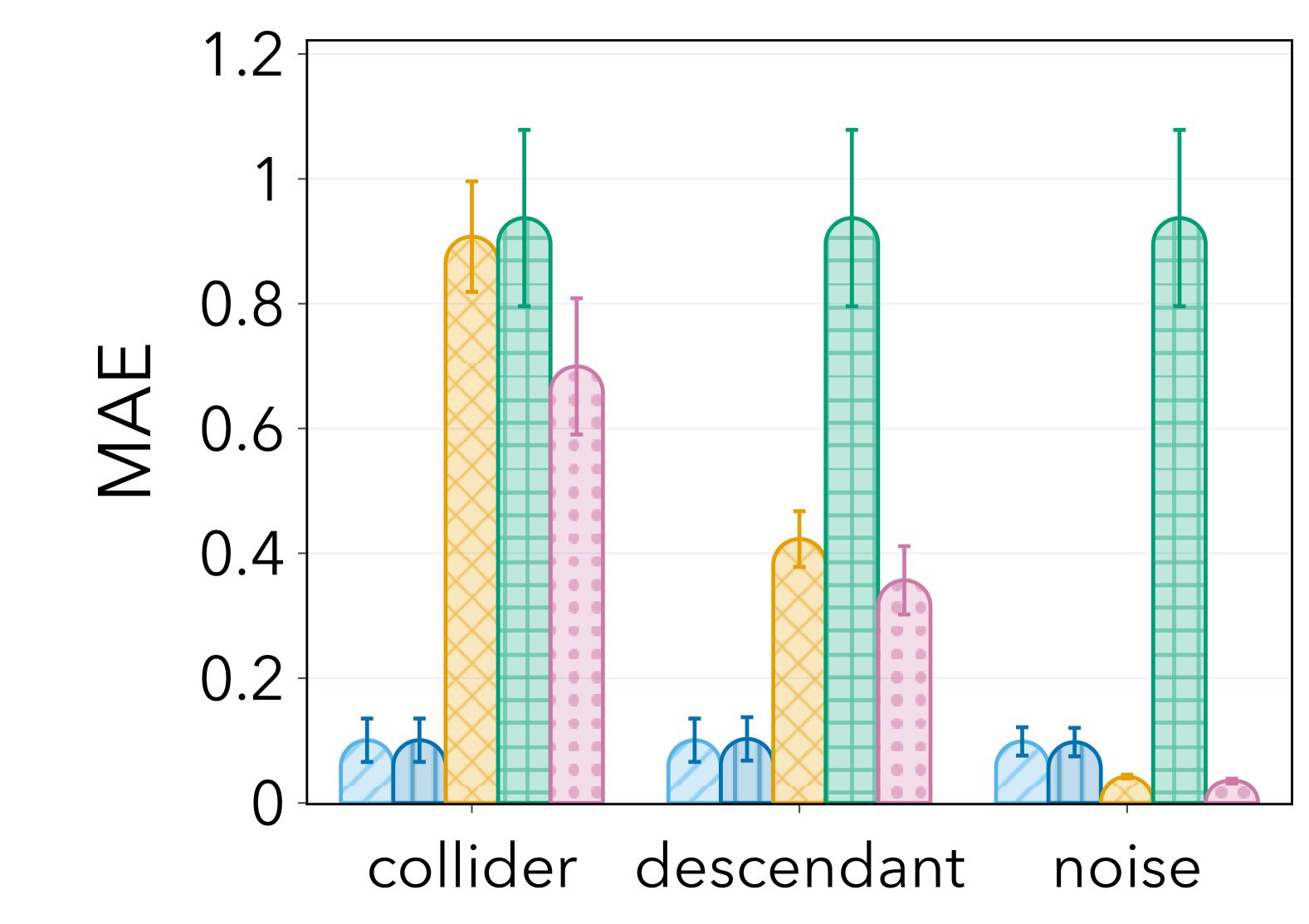
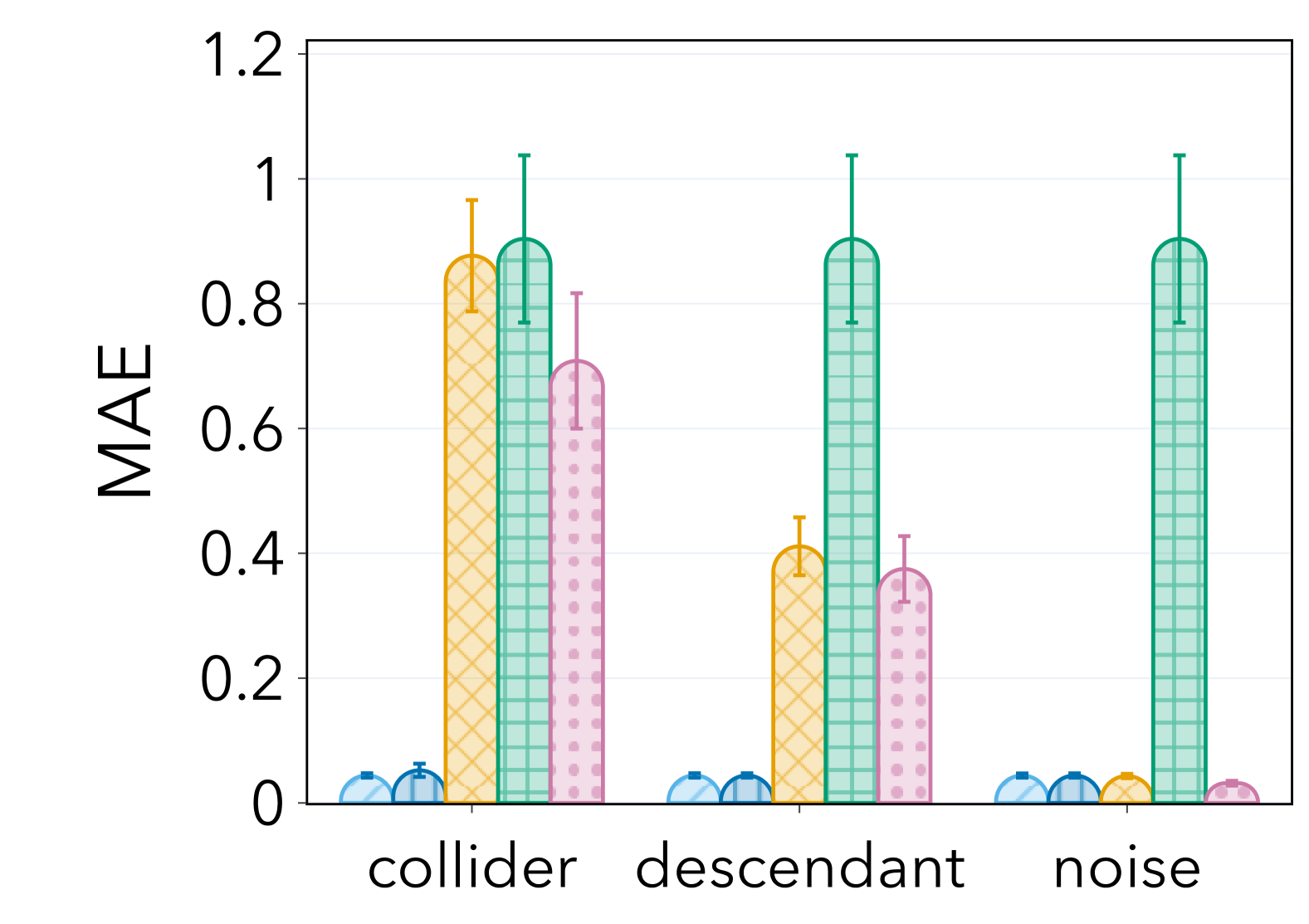
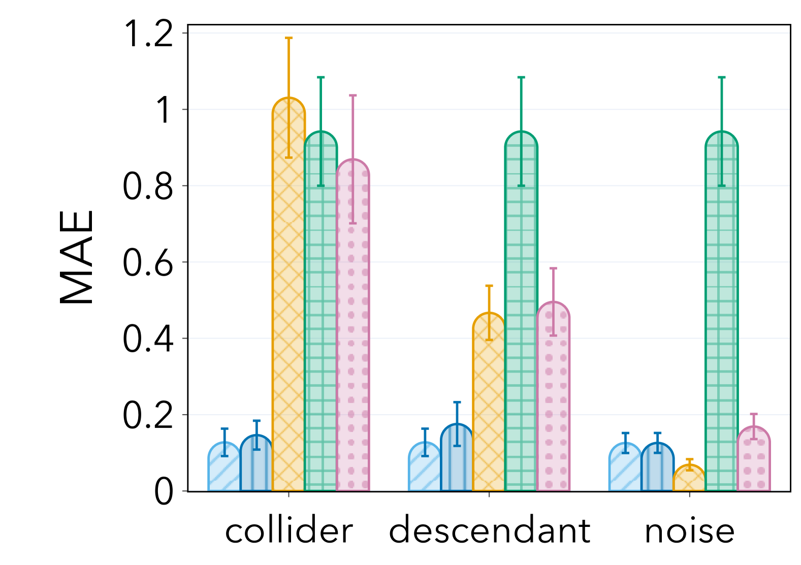
Figure 2: (Top row) Graphical models illustrating three scenarios in which the unobserved confounder $U$ may break different invariances between $T$, $Y$, and the observed covariates $X$. In each graph, dashed arrows denote optional edges, dashed nodes indicate unobserved variables, green and red nodes indicate good and bad controls, respectively. Panel (a) shows the case where $U$ does not break any invariance. Panel (b) shows the case where $U$ breaks the invariance between $X_{p}$ and $T$. Panel (c) shows the case where $U$ breaks the invariance between $X_{p}$ and $Y$. (Bottom row) Mean absolute errors are shown across $5$ environments ($n=2500$, $d=5$ observed covariates), with error bars representing standard errors over 20 runs.

In Figure 2 (Row 1), we present the empirical MAE for all methods on finite-sample experiments that confirm the predictions from theory. First of all, both of our methods, $\hat{\theta}_{\mathrm{\includegraphics[height=3.5pt]{figures/ramen3.png}}}$ and $\hat{\theta}_{\mathrm{insta-\includegraphics[height=3.5pt]{figures/ramen3.png}}}$, consistently achieve lower MAE compared to the baselines in all scenarios. In particular, we observe that the differentiable relaxation of our method does not significantly compromise statistical performance. Further, for T-invariance, the performance of $\hat{\theta}_{\mathrm{irm}}$ deteriorates markedly as expected —e.g. in scenarios where the post-treatment variable is a descendant of $Y$, it performs worse than simply adjusting for all available covariates. In contrast, our approach remains robust even when one of the invariances is compromised. Finally, we observe that relying on T-invariance increases the error across methods, possibly because the adjustment set we recover, the parents of the treatment, leads to a statistically less efficient estimator, c.f. Henckel et al. [34, Corollary 3.4].

5.2 Synthetic experiment with random high dimensional DAGs

We randomly draw a graph from the Erdös-Rényi random graph model with a total number of nodes $p=20$. We do rejection sampling to exclude graphs that either contain mediators—as they violate 3.1—or do not contain at least a confounder. We then assign $Y$ and $T$ to nodes such that the invariance assumption is satisfied for at least one of them (see Section C.3 for additional experiments where other invariances hold), and sample all variables from the resulting DAG via a linear structural causal model except for the treatment variable $T$. We sample $T$ from a Bernoulli distribution with parameter equal to the sigmoid function applied to the function $f$ in the structural equation of $T$ as in Equation 1. We further post-process the graph by adding a node $X_{\mathrm{c}}=Y+T$ to make sure that there is at least one post-treatment covariate. We assign the parents of $T$ or $Y$ (except common parents) to be the set of unobserved covariates $U$, depending on the invariance we want to preserve.

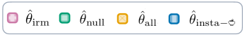
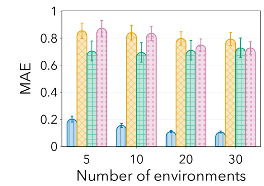
Figure 3: We plot the mean absolute error averaged across environments when the $T$-invariance is preserved. We sample $n=2000$ points for each environment; we report mean and standard error over $100$ runs.

In each environment, we apply a random uniform mean and variance shift to all the nodes in the graph except for $T$ and $Y$ while preserving 4.1; see Section D.1 for further details on the data generation. This process leads to distributions that are guaranteed to satisfy all our assumptions in Theorem 1.

In our experiments we sample 100 DAGs and for each DAG vary the number of environments while keeping the sample size fixed. In Figure 3, we plot the empirical MAE of $\hat{\theta}_{\mathrm{insta-\includegraphics[height=3.5pt]{figures/ramen3.png}}}$ ($\hat{\theta}_{\mathrm{\includegraphics[height=3.5pt]{figures/ramen3.png}}}$ is computationally infeasible) and the baseline estimators averaged across the DAGs as a function of the number of environments. Notably, we observe that across all settings and numbers of available environments, $\hat{\theta}_{\mathrm{insta-\includegraphics[height=3.5pt]{figures/ramen3.png}}}$ significantly outperforms all the other baselines. Expectedly, $\hat{\theta}_{\mathrm{irm}}$ fails to surpass all trivial baselines, even with many environments, as it lacks the robustness to unobserved parents of $Y$.

5.3 Semi-synthetic experiments: IHDP

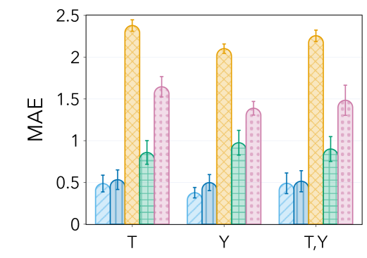
Figure 4: Mean absolute error averaged across environments for the IHDP dataset when different invariances are preserved (T, Y, or both). We consider five environments with $n=748$ points each; mean and standard error are reported over $20$ runs.

The IHDP dataset contains covariates from $n=748$ low-birth-weight, premature infants enrolled in a home visitation program designed to improve their cognitive scores [36]. Instead of using the commonly adopted synthetic functions from Dorie [18], we simulate a non-linear version of the outcome and treatment mechanisms inspired by Kang and Schafer [44]. Specifically, we retain the $6$ continuous covariates (out of $25$ total covariates) from the original dataset and simulate the outcome $Y$ and treatment $T$ by randomly sampling complex functional forms, such as exponentials and polynomials. In addition, we introduce a 2-dimensional synthetic collider, $X_{\mathrm{c}}$, as a linear function of $T$ and $Y$. We generate environments using Gaussian mean shifts in both pre-and post-treatment features, as well as in either $Y$ or $T$ or neither of them, and set the number of environments to $|\mathcal{E}|=5$. Finally, at inference time we do not observe one of the parents of the node among $Y,T$ that is not invariant. See Section D.2 for the experimental details.

Figure 4 depicts the MAE of all the methods when different invariance assumptions hold. Similar to the synthetic experiments in Sections 5.1 and 5.2, $\hat{\theta}_{\mathrm{irm}}$ exhibits higher MAE when $Y$ is not invariant across environments, and $\hat{\theta}_{\mathrm{all}}$, adjusting for all features, generally results in poor performance. Interestingly, $\hat{\theta}_{\mathrm{null}}$ performs competitively since the confounders have a limited impact on the outcome and treatment assignment in this dataset. Additional experiments where the post-treatment feature is either a descendant of the outcome, independent noise, or where neither $T$ nor $Y$ remains invariant are provided in Section C.2. Moreover, we present experiments including mediators between the treatment and the outcome in Section C.1.

5.4 Real-world experiment: effect of maternal smoking on birth weight

Figure 5: ATE estimates for the Cattaneo2 dataset using different baselines. We report the mean and standard deviation over $100$ initializations of the random seeds in the algorithms.

Method	ATE (mean $\pm$ std)
$\hat{\theta}_{\mathrm{null}}$	$-275.25\pm 10^{-5}$
$\hat{\theta}_{\mathrm{all}}$	$-157.55\pm 10^{-5}$
$\hat{\theta}_{\mathrm{irm}}$	$-182.65\pm 48.32$
$\hat{\theta}_{\mathrm{insta-\includegraphics[height=3.5pt]{figures/ramen3.png}}}$	$-214.60\pm 25.20$

In our real-world experiment, we evaluate our method on the observational dataset from [8] that studies the effect of maternal smoking (treatment $T$) during pregnancy on birth weight (outcome $Y$) using the data from $n=4642$ patients. We split the original dataset into $|\mathcal{E}|=4$ environments defined by the trimester of birth. We then use $20$ other variables from the original dataset as observed covariates $X$. Given the nature of the treatment, we expect that some features are post-treatment, i.e. measured after the mother started smoking, as noted in Wilcox [90]. We provide complete experimental details in Section D.3.

Table 5 presents the results of the differentiable version of our method, alongside various baselines. While the ground truth ATE is unknown, the effect estimated by adjusting for the set selected by $\hat{\theta}_{\mathrm{insta-\includegraphics[height=3.5pt]{figures/ramen3.png}}}$ aligns with existing epidemiological literature: both observational and interventional studies [54, 74] as well as statistical analyses [2, 8] estimate a decrease in birth weight that ranges from 200 to 250 grams for infants born to smoking mothers compared to non-smoking mothers. In contrast, $\hat{\theta}_{\mathrm{null}}$ overestimates the ATE, whereas both $\hat{\theta}_{\mathrm{all}}$ and $\hat{\theta}_{\mathrm{irm}}$ underestimate it.

6 Discussion and future work

In this work, we proposed Robust ATE identification from Multiple ENvironments (Ramen), a method that leverages multiple environments to identify the ATE in the presence of post-treatment and unobserved variables. To the best of our knowledge, we present the first ATE identification guarantees in this highly relevant, but previously unexplored setting. Further, we introduce a new version of double robustness that concerns unobserved variables rather than model misspecification.

Nevertheless, our method faces several limitations. First, similar to other kernel-based methods, our approach suffers from the curse of dimensionality and the computational complexity associated with computing kernel matrix. Further, the requirement for sufficient heterogeneity across environments may be too stringent in some practical cases. Finally, the combinatorial subset is computationally demanding, and the Gumbel trick remains a heuristic solution. Addressing any of these shortcomings would be good avenues for future work.

Appendices

The following appendices provide deferred proofs, experiment details, and ablation studies. 1

Table of contents

Appendix A Methodology

A.1 Discussion of 3.2

Figure 6: Although neither full set of parents is observed, one can still find a valid adjustment set $\{X_{1},X_{2}\}$ (depicted in green).

First, we observe here that 3.2 is not a minimal “observability” condition on the parents of $Y$ and $T$: in some cases, it might still be possible to find a valid adjustment set via the observed parents of either $T$ or $Y$ (or both), although no full set of parents was observed (see e.g. Figure 6). However, in such cases, the valid adjustment set or the corresponding regression function cannot be recovered via invariance methods, since neither $T$ nor $Y$ are invariant across environments. Thus, in a way, 3.2 is a minimal assumption on the DAG if one wants to recover the ATE via invariance of conditional expectations.

Further, we remark that our assumption is neither stronger nor weaker than the commonly used ignorability assumption with respect to $X$ [66]. For example, if parents of both $T$ and $Y$ are unobserved, 3.2 will not hold, but ignorability could still apply if no common parent of $T$ and $Y$ is unobserved. Conversely, in graphs with M-bias structures and colliders, the ignorability assumption will not hold.

Below, we give some examples of settings in which 3.2 holds, including scenarios in the existing invariance literature [61, 25]:

Fully observed DAG

In [61], we are given multi-environment data $\{\mathbb{P}^{e}:e\in\mathcal{E}\}$, where each distribution $\mathbb{P}^{e}$ is induced by an SCM $\mathcal{M}^{e}=(\mathcal{G},\{f^{e}_{i}\}_{i=1}^{p},\mathbb{P}^{e}_{\epsilon})$, all variables $(X_{1},...,X_{d},Y)$ are observed, and for all $\mathbb{P}^{e}\in\mathcal{E}$ it is satisfied that

$$Y^{e}=g(X^{e}_{\operatorname{Pa}(Y)},\epsilon^{e}),\epsilon^{e}\sim F_{\epsilon}\text{ and }\epsilon^{e}\perp\!\!\!\perp X^{e}_{\operatorname{Pa}(Y)}.$$

In particular, the independence condition implies equality of conditional distributions $\mathbb{P}^{e}(Y|X^{e}_{\operatorname{Pa}(Y)})$ across environments and thus 3.2(b).

General DAG with additive noise

In [25], the target variable follows the following data generating process for all $e\in\mathcal{E}$:

$$Y^{e}=g(X^{e}_{S^{\star}})+\epsilon^{e};\quad\mathbb{E}[\epsilon^{e}|X^{e}_{S^{\star}}]=0,$$

where $S^{\star}$ is the ”true important variable set”. This setting is, in a way, more general than [61], since the noise variable is not required to be independent of the parent variables—instead, the only condition is on the first conditional moment of $\epsilon^{e}$. Due to the additivity of the noise, 3.2(b) follows immediately.

General DAG with multiplicative noise

We can define a similar setting for multiplicative noise, setting for all $e\in\mathcal{E}$:

$$Y^{e}=g(X^{e}_{S^{\star}})\epsilon^{e};\quad\mathbb{E}[\epsilon^{e}|X^{e}_{S^{\star}}]=c,$$

where $S^{\star}$ is, again, the true parent/important variable set, and $c$ is independent of the environment. We observe that 3.2(b) follows since it holds that

$$\mathbb{E}^{e}[Y|X_{S^{\star}}]=\mathbb{E}^{e}[g(X_{S^{\star}})\epsilon|X_{S^{\star}}]=g(X_{S^{\star}})\mathbb{E}^{e}[\epsilon|X_{S^{\star}}]=cg(X_{S^{\star}}).$$

General DAG with polynomial noise

From the above two examples, it becomes clear that for any $Y=g(X_{S^{\star}})p_{k}(\epsilon)$, where $p$ is a polynomial of degree $k$, we have that 3.2(b) holds if for all $e\in\mathcal{E}$ it holds that

$$\mathbb{E}^{e}[\epsilon^{k^{\prime}}\mid X_{S^{\star}}]=c_{l},\text{ for all }k^{\prime}\leq k.$$

where $S^{\star}$ is the important variable/parent set. This condition is strictly weaker than the independence condition since $k$ is finite.

A.2 Proof of Theorem 1

First, we establish that the loss function in Equation 4 attains a value of zero at any minimizer $S_{\includegraphics[height=3.5pt]{figures/ramen3.png}}$. By 3.2, there exists an invariant node $V\in\{T,Y\}$ whose parents are observed. Since it holds that $J_{\operatorname{Pa}(V)}(Z;V)=0$ and $\operatorname{Pa}(V)\subseteq\mathcal{I}_{V}$, we conclude that there exists a subset $S\subseteq\mathcal{I}_{V}$ such that $\min\{J_{S}(Z;T),J_{S}(Z;Y)\}=0$. Additionally, since the loss function is non-negative, any global minimizer of Equation 4 must have a corresponding loss value of zero.

Recall that the Ramen estimator is given by

$$\theta^{e}(S_{\includegraphics[height=3.5pt]{figures/ramen3.png}}):=\underbracket{\mathbb{E}_{\mathbb{P}^{e}}\left[\bar{\mu}_{1}(X_{S_{\includegraphics[height=2.5pt]{figures/ramen3.png}}})+\frac{(Y-\bar{\mu}_{1}(X_{S_{\includegraphics[height=2.5pt]{figures/ramen3.png}}}))T}{\bar{\pi}(X_{S_{\includegraphics[height=2.5pt]{figures/ramen3.png}}})}\right]}_{T_{1}}-\underbracket{\mathbb{E}_{\mathbb{P}^{e}}\left[\bar{\mu}_{0}(X_{S_{\includegraphics[height=2.5pt]{figures/ramen3.png}}})+\frac{(Y-\bar{\mu}_{0}(X_{S_{\includegraphics[height=2.5pt]{figures/ramen3.png}}}))(1-T)}{1-\bar{\pi}(X_{S_{\includegraphics[height=2.5pt]{figures/ramen3.png}}})}\right]}_{T_{2}}.$$

where we have slightly rearranged the order of the terms. In the following, we only consider the treated term $T_{1}$ and prove that $T_{1}=\mathbb{E}_{\mathbb{P}^{e}}\left[Y^{\operatorname{do}(T=1)}\right]$. Analogous reasoning for the control term $T_{2}$ shows that $T_{2}=\mathbb{E}_{\mathbb{P}^{e}}\left[Y^{\operatorname{do}(T=0)}\right]$ and thus proves the claim.

We now consider two cases, depending on whether the minimum is attained for the node $Y$ or $T$.

Case 1: $J_{S_{\includegraphics[height=2.5pt]{figures/ramen3.png}}}(Z;T)=0$.

Since we assume that the kernel belongs to a universal RKHS [82, Def. 4], it follows from Gretton et al. [24, Theorem 5] that for all $e\in\mathcal{E}$

$$\overline{m}^{e}_{S_{\includegraphics[height=2.5pt]{figures/ramen3.png}}}(Z;T)=\mathbb{E}_{\mathbb{P}^{e}}[T\mid X_{S_{\includegraphics[height=2.5pt]{figures/ramen3.png}}}]=\bar{\pi}\left(X_{S_{\includegraphics[height=2.5pt]{figures/ramen3.png}}}\right),~\mathbb{P}^{e}-\mathrm{a.s}.$$ (8)

Then, by 4.1, it holds that

$$\bar{\pi}(X_{S_{\includegraphics[height=2.5pt]{figures/ramen3.png}}})=\bar{\pi}(Z_{\operatorname{Pa}(T)}),~~\overline{\mathbb{P}}-\mathrm{a.s.}$$

Further, since the measure $\overline{\mathbb{P}}$ dominates $\mathbb{P}^{e}$, it holds that

$$\bar{\pi}(X_{S_{\includegraphics[height=2.5pt]{figures/ramen3.png}}})=\bar{\pi}(Z_{\operatorname{Pa}(T)}),~\mathbb{P}^{e}-\mathrm{a.s.}$$ (9)

Using the tower property, we compute

$$\mathbb{E}_{\mathbb{P}^{e}}\left[\left(1-\frac{T}{\bar{\pi}({X_{S_{\includegraphics[height=2.5pt]{figures/ramen3.png}}}})}\right)\bar{\mu}_{1}(X_{S_{\includegraphics[height=2.5pt]{figures/ramen3.png}}})\right] =\mathbb{E}_{\mathbb{P}^{e}}\left[\bar{\mu}_{1}(X_{S_{\includegraphics[height=2.5pt]{figures/ramen3.png}}})\right]-\mathbb{E}_{\mathbb{P}^{e}}\left[\mathbb{E}_{\mathbb{P}^{e}}\left[\frac{T}{\bar{\pi}({X_{S_{\includegraphics[height=2.5pt]{figures/ramen3.png}}}})}\mid X_{S_{\includegraphics[height=2.5pt]{figures/ramen3.png}}}\right]\bar{\mu}_{1}(X_{S_{\includegraphics[height=2.5pt]{figures/ramen3.png}}})\right]$$

$$=\mathbb{E}_{\mathbb{P}^{e}}\left[\bar{\mu}_{1}(X_{S_{\includegraphics[height=2.5pt]{figures/ramen3.png}}})\right]-\mathbb{E}_{\mathbb{P}^{e}}\left[\bar{\mu}_{1}(X_{S_{\includegraphics[height=2.5pt]{figures/ramen3.png}}})\right]=0.$$

Hence,

$$T_{1}=\mathbb{E}_{\mathbb{P}^{e}}\left[\frac{TY}{\bar{\pi}({X_{S_{\includegraphics[height=2.5pt]{figures/ramen3.png}}}})}\right]=\mathbb{E}_{\mathbb{P}^{e}}\left[\frac{TY}{\bar{\pi}(Z_{\operatorname{Pa}(T)})}\right],$$

where the second equality follows by (9).

Now, under the positivity assumption and Assumption 3.2, since the parents of $T$ satisfy the backdoor criteria, we can identify the treatment effect, that is, it holds that

$$\mathbb{E}_{\mathbb{P}^{e}}\left[\frac{TY}{\bar{\pi}(Z_{\operatorname{Pa}(T)})}\right]=\mathbb{E}_{\mathbb{P}^{e}}\left[Y^{\operatorname{do}(T=1)}\right].$$

Thus, we conclude that

$$\mathbb{E}_{\mathbb{P}^{e}}\left[Y^{\operatorname{do}(T=1)}\right] =\mathbb{E}_{\mathbb{P}^{e}}\left[\frac{TY}{\bar{\pi}(X_{S_{\includegraphics[height=2.5pt]{figures/ramen3.png}}})}+\left(1-\frac{T}{\bar{\pi}(X_{S_{\includegraphics[height=2.5pt]{figures/ramen3.png}}})}\right)\bar{\mu}_{1}(X_{S_{\includegraphics[height=2.5pt]{figures/ramen3.png}}})\right].$$

The analogous argument can be used to show $T_{2}=\mathbb{E}_{\mathbb{P}^{e}}\left[Y^{\operatorname{do}(T=0)}\right]$. Combining the terms yields

$$\theta^{e}(S_{\includegraphics[height=3.5pt]{figures/ramen3.png}})=\mathbb{E}_{\mathbb{P}^{e}}\left[Y^{\operatorname{do}(T=1)}\right]-\mathbb{E}_{\mathbb{P}^{e}}\left[Y^{\operatorname{do}(T=0)}\right].$$

Case 2: $J_{S_{\includegraphics[height=2.5pt]{figures/ramen3.png}}}(Z;Y)=0$.

We recall that this term of the loss function is defined as

$$J_{S}(Z;Y):=\max_{t\in\{0,1\}}\max_{e\in\mathcal{E}}\left(\sup_{h\in L^{0}\left(\mathbb{R}^{|S|}\right)}\mathbb{E}_{\mathbb{P}^{e}}\left[\left(Y-\mathbb{E}_{\overline{\mathbb{P}}}[Y\mid Z_{S},T=t]\right)h(Z_{S})\mid T=t\right]\right)^{2}.$$

Thus, again, by the universal property of the kernel $k$ and Gretton et al. [24, Theorem 5], it follows

$$\forall e\in\mathcal{E}:~~\mathbb{E}_{\mathbb{P}^{e}}[Y\mid T=t,X_{S_{\includegraphics[height=2.5pt]{figures/ramen3.png}}}]=\bar{\mu}_{t}\left(X_{S_{\includegraphics[height=2.5pt]{figures/ramen3.png}}}\right),~~\mathbb{P}^{e}-\mathrm{a.s.,}~~\forall t\in\{0,1\}.$$ (10)

Further, by 4.1, we have

$$\bar{\mu}_{t}(X_{S_{\includegraphics[height=2.5pt]{figures/ramen3.png}}})=\bar{\mu}_{t}(Z_{\operatorname{Pa}(Y)}),~~\overline{\mathbb{P}}-\mathrm{a.s.}$$

This also implies $\mathbb{P}^{e}-\mathrm{a.s.}$ equality of the conditional means for all $e\in\mathcal{E}$ by domination of measure. We now observe that

$$\mathbb{E}_{\mathbb{P}^{e}}\left[\bar{\mu}_{1}(X_{S_{\includegraphics[height=2.5pt]{figures/ramen3.png}}})\right]=\mathbb{E}_{\mathbb{P}^{e}}\left[\bar{\mu}_{1}({Z_{\operatorname{Pa}(Y)}})\right]=\mathbb{E}_{\mathbb{P}^{e}}\left[Y^{\operatorname{do}(T=1)}\right],$$

since $Z_{\operatorname{Pa}(Y)}$ is a valid adjustment set. Then, we simplify the second treatment term in our estimand using the tower property the invariance of the conditional expectation:

$$\mathbb{E}_{\mathbb{P}^{e}}\left[\frac{(Y-\bar{\mu}_{1}(X_{S_{\includegraphics[height=2.5pt]{figures/ramen3.png}}}))T}{\bar{\pi}(X_{S_{\includegraphics[height=2.5pt]{figures/ramen3.png}}})}\right] =\mathbb{E}_{\mathbb{P}^{e}}\left[\frac{1}{\bar{\pi}(X_{S_{\includegraphics[height=2.5pt]{figures/ramen3.png}}})}\mathbb{E}_{\mathbb{P}^{e}}\left[(Y-\bar{\mu}_{1}(X_{S_{\includegraphics[height=2.5pt]{figures/ramen3.png}}}))\mid X_{S_{\includegraphics[height=2.5pt]{figures/ramen3.png}}},T=1\right]\mathbb{P}^{e}(T=1\mid X_{S_{\includegraphics[height=2.5pt]{figures/ramen3.png}}})\right].$$

The RHS is equal to zero since $\mathbb{E}_{\mathbb{P}^{e}}\left[Y\mid X_{S_{\includegraphics[height=2.5pt]{figures/ramen3.png}}},T=1\right]=\bar{\mu}_{1}(X_{S_{\includegraphics[height=2.5pt]{figures/ramen3.png}}})~,\mathbb{P}^{e}-\mathrm{a.s.}$, as the invariance from Equation 10 holds.

With an analogous argument for the control term it follows that

$$\mathbb{E}_{\mathbb{P}^{e}}\left[\frac{(Y-\bar{\mu}_{0}(X_{S_{\includegraphics[height=2.5pt]{figures/ramen3.png}}}))(1-T)}{1-\bar{\pi}(X_{S_{\includegraphics[height=2.5pt]{figures/ramen3.png}}})}\right]=0,$$

and thus, the Ramen estimator is equivalent to the ATE:

$$\theta^{e}(S_{\includegraphics[height=3.5pt]{figures/ramen3.png}})=\mathbb{E}_{\mathbb{P}^{e}}\left[Y^{\operatorname{do}(T=1)}\right]-\mathbb{E}_{\mathbb{P}^{e}}\left[Y^{\operatorname{do}(T=0)}\right].$$

A.3 Implementation details

In this section, we describe all the implementation details for our methodology.

Estimation of the loss function

We have several choices when it comes to estimating our loss function, as there is a trade-off between statistical and computational efficiency. For instance, one can choose the linear time estimator proposed in Gretton et al. [24, Section 6] or the efficient estimator proposed in Kim and Ramdas [46] that runs in quadratic time. In this paper, we estimate

$$\mathbb{H}_{e}^{2}(S):=\mathbb{E}_{\mathbb{P}^{e}}\left[\delta_{S}(Z;V)k\left(Z_{S},\tilde{Z}^{\mathrm{os}}_{S}\right)\delta_{S}(\tilde{V},\tilde{Z}^{\mathrm{os}})\right]$$

using the cross U-statistic from Kim and Ramdas [46], defined as

$$\hat{\mathbb{H}}_{e}^{2}(S):=\frac{2}{n}\sum_{i=1}^{n/2}h_{S}(Z_{i},V_{i}),$$

$$\text{with}~h_{S}(Z_{i},V_{i}):=\frac{2}{n}\sum_{j=n/2+1}^{n}\delta_{S}(Z_{i},V_{i})k(Z_{i,S},Z_{j,S})\delta_{S}(Z_{j},V_{j}).$$

Moreover, we would like the two loss functions, i.e., $J_{Y}$ and $J_{T}$, to be on the same scale to avoid any finite sample issues. Therefore, we standardize the cross U-statistic by dividing the empirical variance $\hat{\sigma}\left(\hat{\mathbb{H}}_{e}^{2}(S)\right)$, i.e. the finite sample estimate of the variance term

$$\sigma^{2}\left(\hat{\mathbb{H}}_{e}^{2}(S)\right):=\mathbb{E}_{\mathbb{P}^{e}}\left[\left(h_{S}(Z)-\mathbb{E}_{\mathbb{P}^{e}}\left[h_{S}(Z)\right]\right)^{2}\right].$$

Choice of kernel

An important issue in practice is the selection of the kernel parameters. We used a Gaussian kernel in all of our experiments. We set the bandwidth of the kernel $\sigma$ to be the median distance between points $X$ in the pooled sample—this remains a heuristic similar to those described in Takeuchi et al. [83], and the optimum kernel choice is an ongoing area of research.

A.3.1 Algorithm 1: Combinatorial search over subsets

We now describe the concrete implementation of our first algorithm.

Since we know that $T$ is a parent of $Y$, we can simplify our loss function to incorporate this knowledge. Let us define the quantity $\delta_{y,t}(X_{S},Y):=Y-\bar{\mu}_{t}(X_{S})$, where $\bar{\mu}_{t}(X_{S}):=\mathbb{E}_{\overline{\mathbb{P}}}[Y\mid X_{S},T=t]$. We can rewrite the Y-invariance loss function as follows

$$\min_{S\subseteq[d]}~\max_{e\in\mathcal{E},t\in\{0,1\}}~\mathbb{E}_{\mathbb{P}^{e}}\left[\delta_{y,t}(Y,X_{S})k\left(X_{S},X^{\prime}_{S}\right)\delta_{y,t}(Y^{\prime},X^{\prime}_{S})\mid T=t\right].$$

Similarly, we define $\bar{\pi}(X_{S}):=\mathbb{E}_{\overline{\mathbb{P}}}[T\mid X_{S}]$ and minimize the T-invariance loss function

$$\min_{S\subseteq[d]}~\max_{e\in\mathcal{E}}~\mathbb{E}_{\mathbb{P}^{e}}\left[\delta_{t}(T,X_{S})k\left(X_{S},X^{\prime}_{S}\right)\delta_{t}(T^{\prime},X^{\prime}_{S})\right].$$

where $\delta_{t}(X_{S},T):=T-\bar{\pi}(X_{S})$.

Algorithm 1 Combinatorial search over subsets ($\hat{\theta}_{\mathrm{\includegraphics[height=3.5pt]{figures/ramen3.png}}}$)

1:Input: Data $\{(X_{e},Y_{e},T_{e})\}_{i=1}^{n_{e}}$, Nuisance functions: $\bar{\pi}$, $\bar{\mu}_{0}$, $\bar{\mu}_{1}$

2:for each subset $S\subseteq[d]$ do

3:  for each environment $e\in\mathcal{E}$ do

4:   Compute T-invariance loss using dataset $D^{e}$:

$$\hat{J}_{S}(D^{e};T) \leftarrow\frac{4}{n^{2}}\sum_{i=1}^{n/2}\sum_{j=n/2+1}^{n}(T_{i}-\bar{\pi}(X_{i}))k(X_{i,S},X_{j,S})(T_{j}-\bar{\pi}(X_{j}))$$

$$\hat{J}_{S}(D^{e};T) \leftarrow\frac{\hat{J}_{S}(D^{e};T)}{\widehat{\operatorname{Var}}\left(\hat{J}_{S}(D^{e};T)\right)}$$

5:   Compute Y-invariance loss using dataset $D^{e}$ restricted to samples with $T=1$:

$$\hat{J}_{S}(D^{e};Y_{1}) \leftarrow\frac{4}{n^{2}}\sum_{i=1}^{n/2}\sum_{j=n/2+1}^{n}(Y_{i}-\bar{\mu}_{1}(X_{i}))k(X_{i,S},X_{j,S})(Y_{j}-\bar{\mu}_{1}(X_{j}))$$

$$\hat{J}_{S}(D^{e};Y_{1}) \leftarrow\frac{\hat{J}_{S}(D^{e};Y_{1})}{\widehat{\operatorname{Var}}\left(\hat{J}_{S}(D^{e};Y_{1})\right)}$$

6:   Compute Y-invariance loss using dataset $D^{e}$ restricted to samples with $T=0$:

$$\hat{J}_{S}(D^{e};Y_{0}) \leftarrow\frac{4}{n^{2}}\sum_{i=1}^{n/2}\sum_{j=n/2+1}^{n}(Y_{i}-\bar{\mu}_{0}(X_{i}))k(X_{i,S},X_{j,S})(Y_{j}-\bar{\mu}_{0}(X_{j}))$$

$$\hat{J}_{S}(D^{e};Y_{0}) \leftarrow\frac{\hat{J}_{S}(D^{e};Y_{0})}{\widehat{\operatorname{Var}}\left(\hat{J}_{S}(D^{e};Y_{0})\right)}$$

7:  end for

8:  Compute the worst environment losses:

$$\hat{J}_{S}(T)\leftarrow\max_{e\in\mathcal{E}}J_{S}(D^{e};T),~~\hat{J}_{S}(Y_{1})\leftarrow\max_{e\in\mathcal{E}}J_{S}(D^{e};Y_{1}),~~\hat{J}_{S}(Y_{0})\leftarrow\max_{e\in\mathcal{E}}J_{S}(D^{e};Y_{0})$$

9:end for

10:Return: $S_{\includegraphics[height=3.5pt]{figures/ramen3.png}}\leftarrow\operatorname{argmin}_{S}~\min\left(\hat{J}_{S}(T),\max(\hat{J}_{S}(Y_{1}),\hat{J}_{S}(Y_{0}))\right)$

We show how to compute the adjustment set explicitly in Algorithm 1, assuming oracle access to the nuisance functions. In practice, nuisance functions can be estimated using the pooled data from all environments.

A.3.2 Algorithm 2: Gumbel trick

To deal with the computational infeasibility of searching over all possible subsets of covariates, we propose a continuous relaxation of the optimization problem that can be efficiently solved using gradient descent. The method involves using Gumbel sampling to create differentiable binary masks for covariate selection, which allows optimization via gradient descent. We present the continuous relaxation in Algorithm 2 for obtaining the invariance loss with respect to the node $T$ and $Y$. In this algorithm, we replace the max operator over the environments with an average to obtain a smoother loss function.

Algorithm 2 Gumbel trick for subset selection ($\hat{\theta}_{\mathrm{insta-\includegraphics[height=3.5pt]{figures/ramen3.png}}}$)

1:Input: Data $\{(X_{e},Y_{e},T_{e})\}_{e\in\mathcal{E}}$, temperatures $\tau_{\text{init}},\tau_{\text{final}}$, $k$, $\alpha<1$, learning rates $\eta_{\text{gate}},\eta_{\text{nn}}$, epochs $n_{\text{epochs}}$

2:Initialize gate weights $w_{\pi},w_{y}$ and neural networks $\theta_{\pi},\theta_{y_{1}},\theta_{y_{0}}$; Set $\tau\leftarrow\tau_{\text{init}}$

3:for epoch $=1$ to $n_{\text{epochs}}$ do

4:  if $\text{epoch}\bmod k=0$ then

5:   Update temperature: $\tau\leftarrow\max(\tau_{\text{final}},\tau\cdot\alpha)$

6:  end if

7:  for each environment $e\in\mathcal{E}$ do

8:   Compute masks:

$$B_{j}^{\pi} =\operatorname{sigmoid}((w_{\pi,j}+G_{1,j}-G_{2,j})/\tau)\quad\text{with }G_{1,j},G_{2,j}\sim\text{Gumbel}(0,1)$$

$$B_{j}^{y} =\operatorname{sigmoid}((w_{y,j}+G_{1,j}-G_{2,j})/\tau)\quad\text{with }G_{1,j},G_{2,j}\sim\text{Gumbel}(0,1)$$

9:   Compute invariance losses:

$$\hat{J}_{w_{\pi}}(D^{e};T) \leftarrow\frac{4}{n^{2}}\sum_{i=1}^{n/2}\sum_{j=n/2+1}^{n}(T_{i}-f_{\theta_{\pi}}(X_{i,B^{\pi}}))k(X_{i,B^{\pi}},X_{j,B^{\pi}})(T_{j}-f_{\theta_{\pi}}(X_{j,B^{\pi}}))$$

$$\hat{J}_{w_{\pi}}(D^{e};T) \leftarrow\frac{\hat{J}_{w_{\pi}}(D^{e};T)}{\widehat{\operatorname{Var}}\left(\hat{J}_{w_{\pi}}(D^{e};T)\right)}$$

$$\hat{J}_{w_{y}}(D^{e};Y_{1}) \leftarrow\frac{4}{n^{2}}\sum_{i=1}^{n/2}\sum_{j=n/2+1}^{n}(Y_{i}-f_{\theta_{y_{1}}}(X_{i,B^{y}}))k(X_{i,B^{y}},X_{j,B^{y}})(Y_{j}-f_{\theta_{y_{1}}}(X_{j,B^{y}}))\quad\text{(using $D^{e}$ with $T=1$)}$$

$$\hat{J}_{w_{y}}(D^{e};Y_{1}) \leftarrow\frac{\hat{J}_{w_{y}}(D^{e};Y_{1})}{\widehat{\operatorname{Var}}\left(\hat{J}_{w_{y}}(D^{e};Y_{1})\right)}$$

$$\hat{J}_{w_{y}}(D^{e};Y_{0}) \leftarrow\frac{4}{n^{2}}\sum_{i=1}^{n/2}\sum_{j=n/2+1}^{n}(Y_{i}-f_{\theta_{y_{0}}}(X_{i,B^{y}}))k(X_{i,B^{y}},X_{j,B^{y}})(Y_{j}-f_{\theta_{y_{0}}}(X_{j,B^{y}}))\quad\text{(using $D^{e}$ with $T=0$)}$$

$$\hat{J}_{w_{y}}(D^{e};Y_{0}) \leftarrow\frac{\hat{J}_{w_{y}}(D^{e};Y_{0})}{\widehat{\operatorname{Var}}\left(\hat{J}_{w_{y}}(D^{e};Y_{0})\right)}$$

10:  end for

11:  Compute losses:

$$\hat{J}_{w_{\pi}}\leftarrow\frac{1}{|\mathcal{E}|}\sum_{e}\hat{J}_{w_{\pi}}(D^{e};T),\quad\hat{J}_{w_{y}}\leftarrow\frac{1}{2|\mathcal{E}|}\sum_{e}\hat{J}_{w_{y}}(D^{e};Y_{1})+\hat{J}_{w_{y}}(D^{e};Y_{0})$$

12:  Update parameters:

$$w_{\pi} \leftarrow w_{\pi}-\eta_{\text{gate}}\nabla_{w_{\pi}}\hat{J}_{w_{\pi}},~~\theta_{\pi}\leftarrow\theta_{\pi}-\eta_{\text{nn}}\nabla_{\theta_{\pi}}\hat{J}_{w_{\pi}}$$

$$w_{y} \leftarrow w_{y}-\eta_{\text{gate}}\nabla_{w_{y}}\hat{J}_{w_{y}},~~\theta_{y_{1}}\leftarrow\theta_{y_{1}}-\eta_{\text{nn}}\nabla_{\theta_{y_{1}}}\hat{J}_{w_{y}},~~\theta_{y_{0}}\leftarrow\theta_{y_{0}}-\eta_{\text{nn}}\nabla_{\theta_{y_{0}}}\hat{J}_{w_{y}}$$

13:end for

14:Determine subsets: $S_{T}\leftarrow\{i:w_{\pi,i}>0\}$, $S_{Y}\leftarrow\{i:w_{y,i}>0\}$

15:Calculate exact losses (as defined in Algorithm 1) for each subset $S\in\{S_{T},S_{Y}\}$:

$$J_{S}(T)\leftarrow\frac{1}{|\mathcal{E}|}\sum_{e}\hat{J}_{S}(D^{e};T),~~J_{S}(Y_{1})\leftarrow\frac{1}{|\mathcal{E}|}\sum_{e}\hat{J}_{S}(D^{e};Y_{1}),~~J_{S}(Y_{0})\leftarrow\frac{1}{|\mathcal{E}|}\sum_{e}\hat{J}_{S}(D^{e};Y_{0})$$

16:Return: $S_{\mathrm{insta}-\includegraphics[height=3.5pt]{figures/ramen3.png}}\leftarrow\operatorname{argmin}_{S\in\{S_{T},S_{Y}\}}\min(J_{S}(T),\max(J_{S}(Y_{1}),J_{S}(Y_{0})))$

Appendix B Extended related work

We discuss here the different challenges associated with the problem of identifying and estimating treatment effects. Our focus is to highlight differences and similarities with our methodology—we leave out the orthogonal problem of statistical efficiency for the sake of clarity, and we refer the reader to Guo et al. [27], Cheng et al. [12] for a complete survey of methods.

Covariate selection with pre-treatment covariates

Several works have relaxed the causal sufficiency assumption, allowing for unobserved variables—as long as they are not confounders—while constraining all observed covariates to be pre-treatment. In this setting, the main challenge is M-bias [81], which makes adjusting for the full set of covariates not a viable solution. For instance, EHS [20] was one of the first methods to obtain partial identification of treatment effects in this setting, however, at the cost of computational inefficiency. Gultchin et al. [26] propose a more efficient relaxation for EHS to circumvent the computational inefficiency. Further, several more recent works leverage anchor variables to obtain point identification in a computationally efficient way [9, 11, 75]. In contrast, our setting is different since we do not assume that all observed covariates are pre-treatment.

Covariate selection under causal sufficiency

When all the variables in the causal graph are observed, the only challenge towards identifiability is the presence of post-treatment covariates that can introduce collider bias. Several methods have been proposed to tackle this setting—e.g. IDA [50] and its variants [59, 21] aim to learn a complete graph from data and then infer a valid adjustment set from it to achieve identifiability. However, they suffer from computational inefficiency since they must first learn the entire causal graph, and they only achieve partial identification. More recently, Shi et al. [79] consider the setting where multiple environments are available and apply invariant risk minimization (IRM) [3] for treatment effect estimation. However, it is widely known that IRM requires many environments—linear in the number of covariates—to generalize well even in the linear regime [70]. Finally, Wang et al. [87] recently proposed a reinforcement learning approach to identify the treatmente effect. In contrast, our approach achieves point identification while being computationally efficient and not requiring causal sufficiency.

Identifiability in linear Gaussian SCMs

In linear Gaussian structural causal models (SCMs), the structure of the causal graph imposes algebraic relationships among the entries in the covariance matrix of the associated distribution. Many researchers have exploited these relationships to derive graphical criteria for the identifiability of causal effects, even when some confounders remain unobserved. Specifically, several graphical criteria have been identified for deciding whether, in a given causal graph, a specific causal effect can be identified from the covariance matrix for almost all linear Gaussian SCMs compatible with the graph [19, 22, 88, 6]. In contrast, our approach does not assume linearity or Gaussianity, and instead, we leverage access to multiple heterogeneous data sources for identification.

Combining data from multiple environments

Given the challenges associated with estimating treatment effects using non-randomized data, several works propose detecting bias in the treatment effect estimated from observational data by leveraging randomized trials [92, 56, 38, 39, 17, 15, 14], or multiple observational studies [45, 53]. In contrast, we leverage the heterogeneity across multiple data sources to identify and estimate treatment effects in settings without unobserved confounders.

Appendix C Additional experiments

C.1 Robustness to mediators

We study here the robustness of our method to violations of 3.1. More concretely, we show how the inclusion of a mediator between $T$ and $Y$ affects the ATE estimate for our method and the baselines in several settings. We consider the semi-synthetic experiment setup from Section 5.3, using a 2-dimensional descendant of $Y$ as the post-treatment variable. In Figure 7, we present results for two settings: when the treatment or the outcome is invariant across environments (complete experimental details in Section D.2). All baselines show slightly worse performance when a mediator is included. When $T$ is invariant, our method remains competitive and outperforms the baselines, as the parents of $T$ still form a valid adjustment set despite the mediator. However, both $\hat{\theta}_{\mathrm{\includegraphics[height=3.5pt]{figures/ramen3.png}}}$ and $\hat{\theta}_{\mathrm{insta-\includegraphics[height=3.5pt]{figures/ramen3.png}}}$ experience a significant drop in performance in the $Y$-invariance setup, i.e. when $T$-invariance is violated. This is expected, as in this scenario, we recover the parents of $Y$, which unfortunately also includes the mediator. A closer inspection of the selected subsets reveals that they usually include the mediator, thus failing to estimate the full effect of $T$ on $Y$. Instead, our method recovers the natural direct effect of $T$ on $Y$ [58].

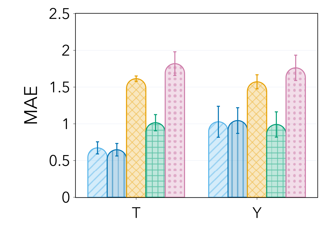
(a) With mediator

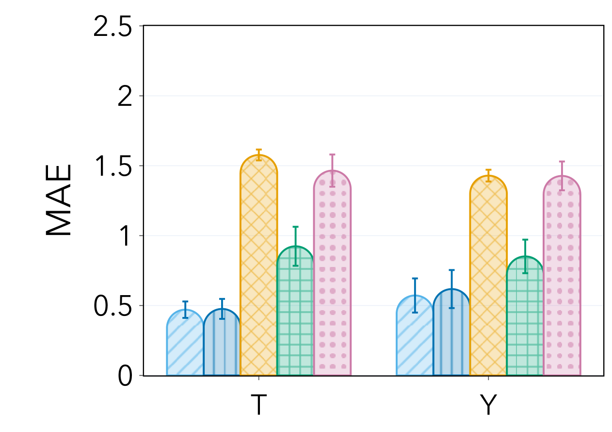
(b) Without mediator

Figure 7: Mean absolute error averaged across environments for the IHDP dataset with a descendant of the outcome $Y$ when different invariances are preserved ($T$ or $Y$). We consider the setting with (a) a mediator between $T$ and $Y$ and (b) without a mediator. We consider five environments with $n=748$ points each; mean and standard error are reported over $20$ runs.

C.2 Robustness to lack of invariance

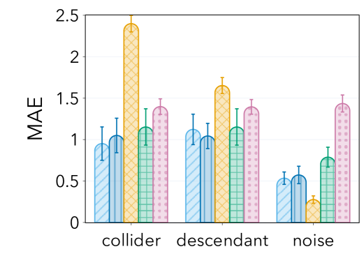
Figure 8: Mean absolute error averaged across environments for the IHDP dataset when no invariance is preserved. We consider five environments with $n=748$ points each; mean and standard error are reported over $20$ runs.

Next, we examine the robustness of our method to violations of the invariance in 3.2. Specifically, we consider again the semi-synthetic experiments of Section 5.3 in the scenario where neither $T$- nor $Y$-invariance holds and there are post-treatment variables (i.e. not the independent noise setting). We provide the results in Figure 8. The performance of our method significantly worsens in this setting, with performance close to the $\hat{\theta}_{\mathrm{null}}$ baseline, as it often recovers the empty set when no invariant node is present. Nonetheless, our method still outperforms $\hat{\theta}_{\mathrm{irm}}$ in all the settings considered.

C.3 Additional random graphs experiments

In Figure 9 (Row 1), we report the MAE averaged across environments for all the invariance settings. First, we observe that across all settings and numbers of available environments, our method significantly outperforms existing baselines. Most notably, $\hat{\theta}_{\mathrm{insta-\includegraphics[height=3.5pt]{figures/ramen3.png}}}$ achieves relatively small errors even with a limited number of environments. In contrast, $\hat{\theta}_{\mathrm{irm}}$ requires a much larger number of environments to outperform the trivial baselines $\hat{\theta}_{\mathrm{null}}$ and $\hat{\theta}_{\mathrm{all}}$. Further, when the parents of $Y$ are unobserved, $\hat{\theta}_{\mathrm{irm}}$ fails to surpass all trivial baselines, even with many environments—this outcome is expected, as the $Y$-invariance is broken in this case and $\hat{\theta}_{\mathrm{irm}}$ lacks the double robustness.

C.4 Additional semi-synthetic experiments

We present the complete experimental results using the IHDP dataset (see Section 5.3) in Figure 9 (Row 2). Specifically, we evaluate our proposed method and the baselines under three conditions, where the two-dimensional variable $X_{c}$ acts as a collider (as described in the main text), descendant, or independent noise. For $T$-, $Y$-, and $T,Y$- invariance, the results align with those obtained in previous sections for linear synthetic experiments. Both $\hat{\theta}_{\mathrm{\includegraphics[height=3.5pt]{figures/ramen3.png}}}$ and its differentiable approximation, $\hat{\theta}_{\mathrm{insta-\includegraphics[height=3.5pt]{figures/ramen3.png}}}$, outperform the baselines in most settings. The sole exception is when the post-treatment variables are independent noise, where $\hat{\theta}_{\mathrm{all}}$ achieves the best performance. In the case of $T$-invariance, both our method and $\hat{\theta}_{\mathrm{irm}}$ exhibit slightly worse performance. $\hat{\theta}_{\mathrm{irm}}$ generally underperforms, showing the highest error even under the independent noise setting. The $\hat{\theta}_{\mathrm{null}}$ baseline demonstrates competitive performance overall, likely due to the relatively low influence of confounders in this setup.

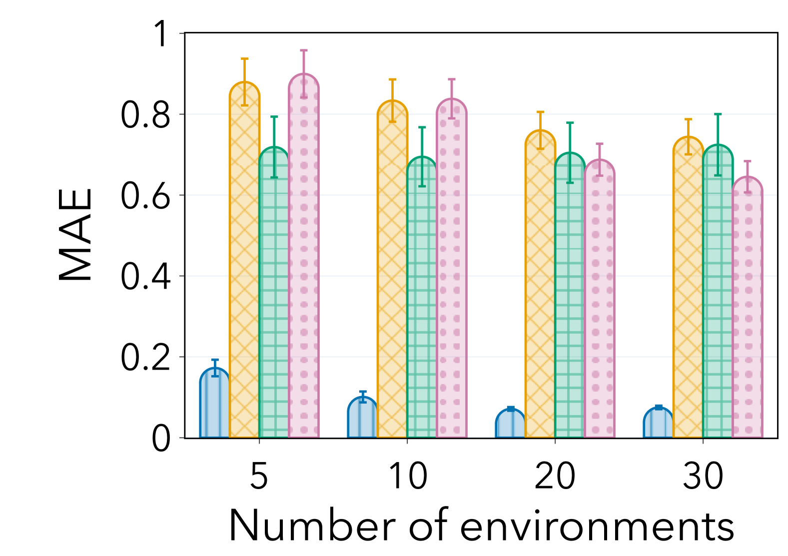
(a) T,Y-invariance

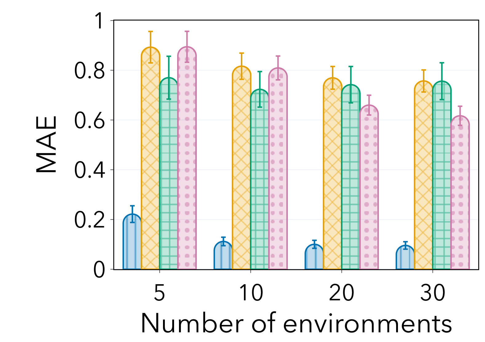
(b) Y-invariance

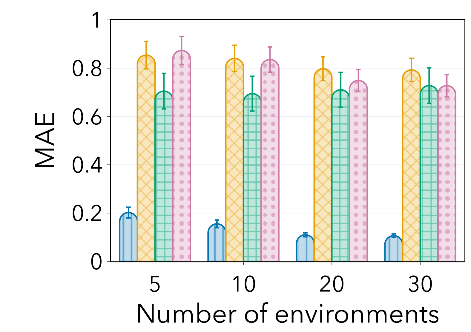
(c) T-invariance

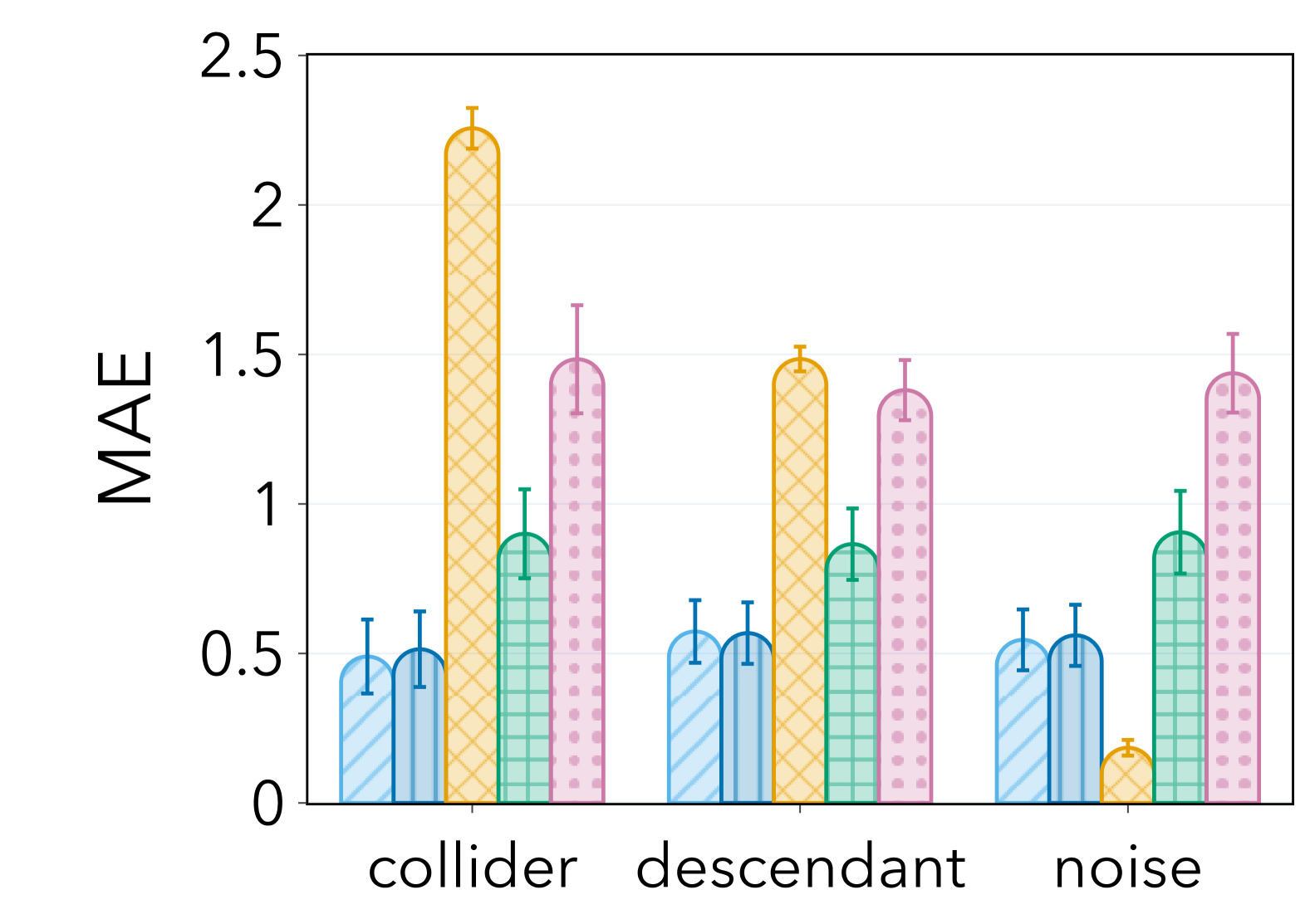
(d) T,Y-invariance

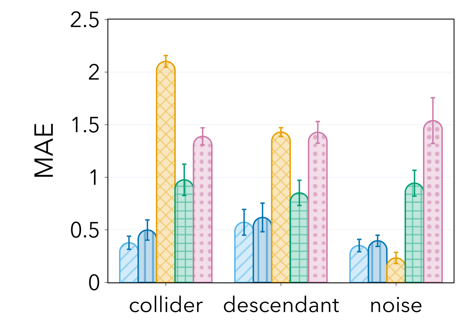
(e) Y-invariance

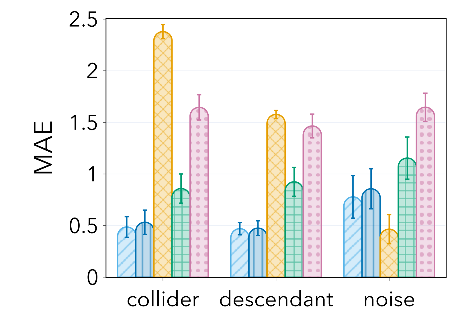
(f) T-invariance

Figure 9: (Top Row) We plot the mean absolute error averaged across environments when: (a) no unobserved variables and both invariance w.r.t $T$ and $Y$ are preserved; (b) the parents of $T$ are unobserved but the invariance w.r.t. $Y$ is preserved; (c) the parents of $Y$ are unobserved but the invariance w.r.t $T$ is preserved. For all plots, we sample $n=2000$ points for each environment; we report mean and standard error over $100$ runs. (Bottom Row) Complete experimental results for the semi-synthetic setup described in Section 5.3 using the IHDP dataset. The plots show the mean absolute error averaged across environments for: (a) both $T$- and $Y$-invariance, (b) $Y$-invariance only, (c) $T$-invariance only.We consider five environments with $n=748$ points each; mean and standard error are reported over $20$ runs.

C.5 Robustness to small sample size

In Figure 10 (a–c), we report the MAE averaged across environments for the three graphical models introduced in Figure 2 (Row 2). We can observe that our method remains competitive even in the small sample size regime: our method consistently outperforms all baselines when a collider or descendant is present. However, its performance declines in the edge case where the post-treatment variable is independent noise.

C.6 Robustness to violations of 4.1

We evaluate here the robustness of our method against violations of our identification condition (i.e. 4.1). To do so, we slightly modify the synthetic experiments presented in Figure 2: We introduce a parameter $\epsilon^{2}$ to control environment heterogeneity. If $\epsilon^{2}=0$, $X$ has the same distribution across environments. Therefore, there is no heterogeneity across environments, and 4.1 is violated. On the other hand, if $\epsilon^{2}>0$ , the mean and variance of $X$ will shift across environments, with larger shifts as the parameter $\epsilon^{2}$ increases. Therefore, the heterogeneity across environments increases with $\epsilon^{2}$, and 4.1 is more likely to be satisfied.

Example C.1 (Post-treatment variables).

Let $\mathcal{E}$ be the collection of environment indices. For each environment $e\in\mathcal{E}$, we first sample $U\sim\mathcal{N}(0,\epsilon^{2}I_{d+1})$. Then, the data is given by

$$\begin{split}\quad X_{p,i}&\sim\mathcal{N}(U_{i},0.5+U^{2}_{i}),~~\text{for}~~i=1,\ldots,d-1;\\ T&\sim\operatorname{Ber}\left(\sigma\left(\beta^{\top}_{t}X_{p}+\epsilon_{t}\right)\right),~~\text{with}~~\beta_{t}\sim\mathcal{N}(0,I_{d-1})~~\text{and}~~\epsilon_{t}\sim\mathcal{N}(U_{d},0.5+U_{d}^{2});\\ Y&=T+\beta^{\top}_{y}X_{p}+\epsilon_{y},~~\text{with}~~\beta_{y}\sim\mathcal{N}(0,I_{d-1})~~\text{and}~~\epsilon_{y}\sim\mathcal{N}(0,1);\\ X_{c}&=a\cdot T+b\cdot Y+\epsilon_{c},~~\text{with}~~\epsilon_{c}\sim\mathcal{N}(U_{d+1},0.5+U_{d+1}^{2}).\end{split}$$

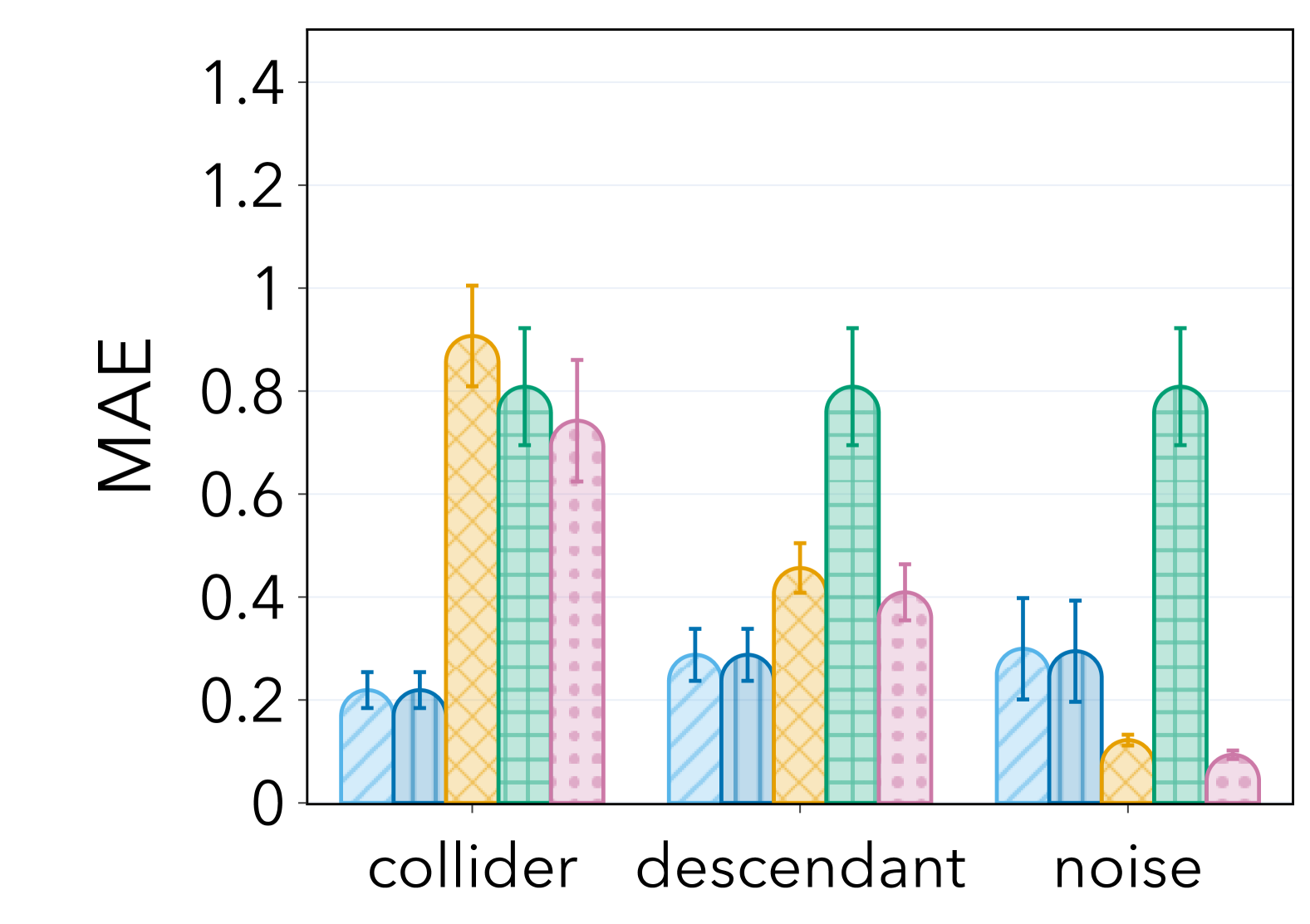
(a) T,Y-invariance

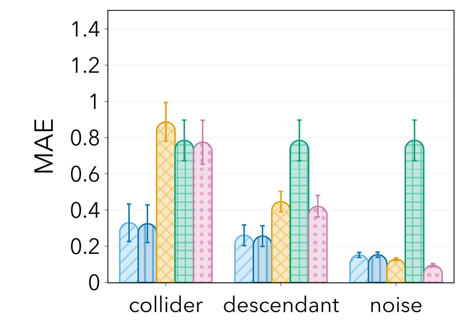
(b) Y-invariance

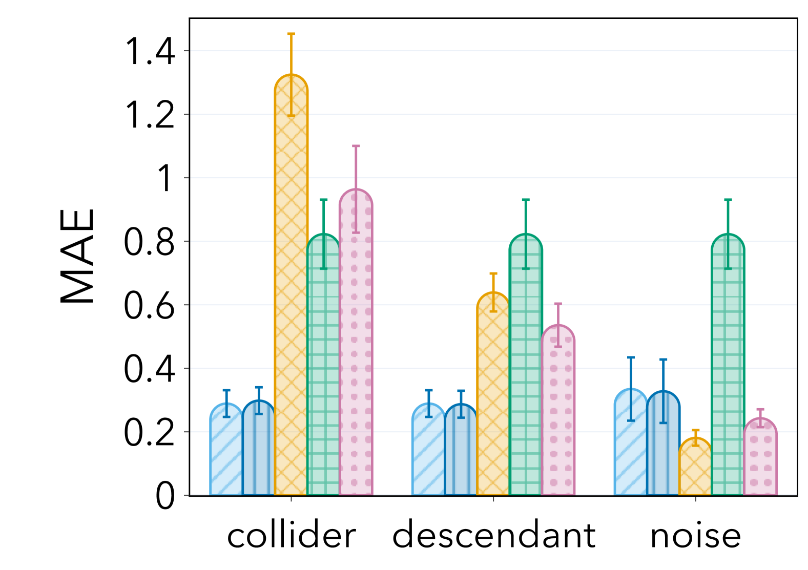
(c) T-invariance

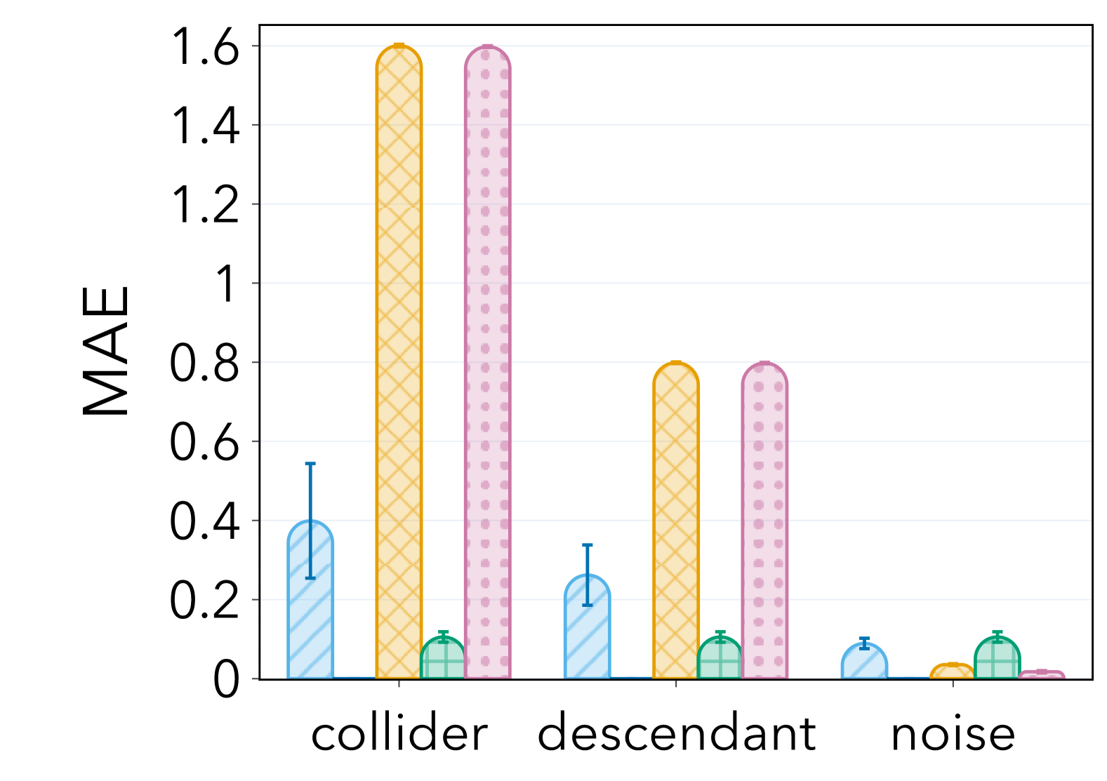
(d) $\epsilon=0.0$

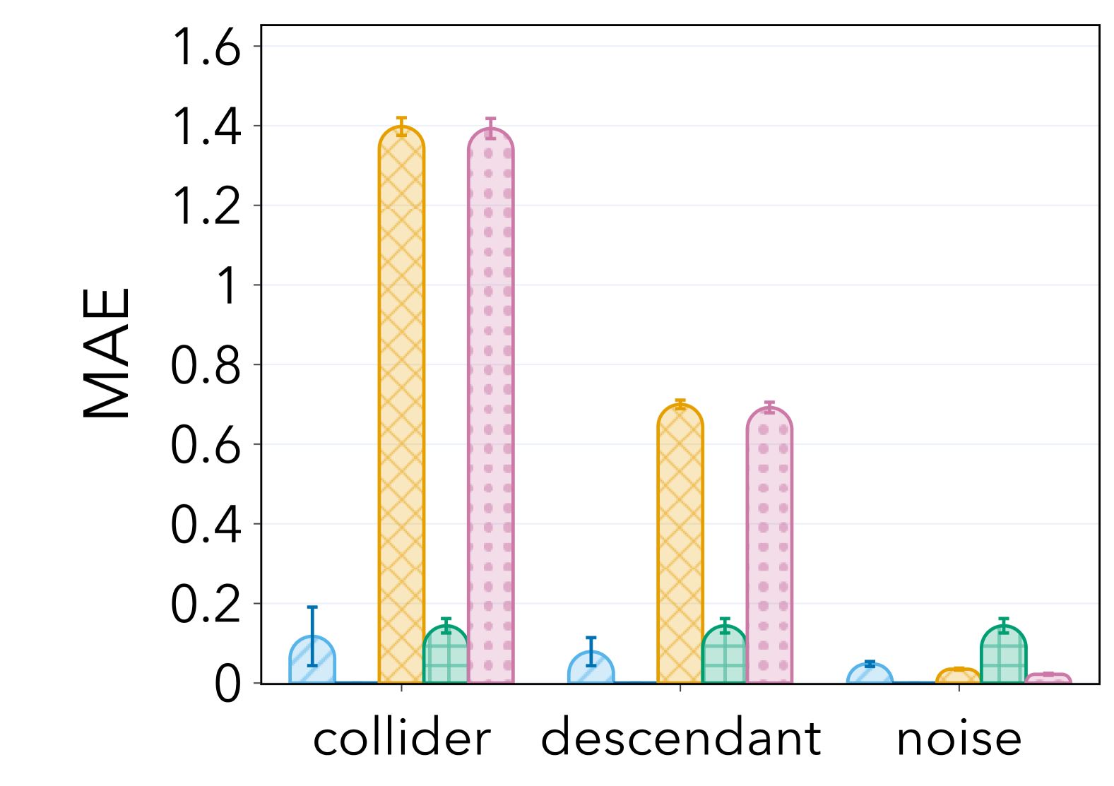
(e) $\epsilon=0.3$

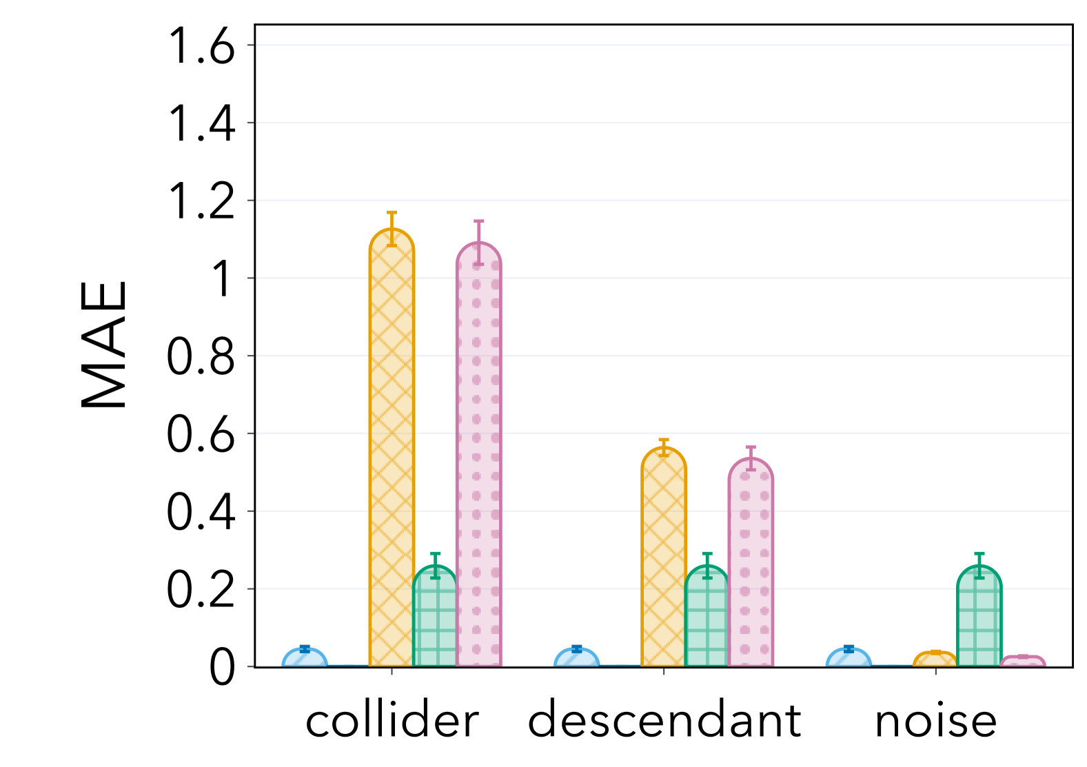
(f) $\epsilon=0.5$

Figure 10: (Row 1) For all the plots: $n=250$, $d=3$, $|\mathcal{E}|=5$. We plot the mean absolute error averaged across environments when: (a) both invariances are preserved; (b) the invariance w.r.t $Y$ is preserved; (c) the invariance w.r.t $T$ is preserved. We report mean and standard error over 20 runs. (Row 2) For all the plots: $n=2500$, $d=3$, $|\mathcal{E}|=5$, and only the invariant w.r.t $Y$ is preserved. We plot the mean absolute error averaged across environments for different levels of heterogeneity in the data (higher $\epsilon$ corresponds to more heterogeneous data).

In Figure 10 (d–f), we plot the MAE for different levels of heterogeneity in the data. We can observe that both $\hat{\theta}_{\mathrm{\includegraphics[height=3.5pt]{figures/ramen3.png}}}$ and $\hat{\theta}_{\mathrm{irm}}$ suffer significantly when there is no heterogeneity ($\epsilon=0.0$). Nevertheless, our method $\hat{\theta}_{\mathrm{\includegraphics[height=3.5pt]{figures/ramen3.png}}}$ consistently outperforms $\hat{\theta}_{\mathrm{irm}}$, even under strong violations of the identification condition. Moreover, $\hat{\theta}_{\mathrm{\includegraphics[height=3.5pt]{figures/ramen3.png}}}$ remains competitive against all baselines when 4.1 is only weakly satisfied ($\epsilon=0.3$).

Appendix D Experimental details

Given an adjustment set, we estimate the ATE for each environment $e\in\mathcal{E}$ as follows

$$\hat{\theta}_{S}^{e}=\frac{1}{n}\sum_{(X_{i},T_{i},Y_{i})\in D^{e}}\hat{\mu}_{S}^{e}(X_{i},1)-\hat{\mu}_{S}^{e}(X_{i},0)+\frac{(Y_{i}-\hat{\mu}_{S}^{e}(X_{i},1))T_{i}}{\hat{\pi}_{S}^{e}(X_{i})}-\frac{(Y_{i}-\hat{\mu}_{S}^{e}(X_{i},0))(1-T_{i})}{1-\hat{\pi}_{S}^{e}(X_{i})},$$

where $\hat{\mu}_{S}^{e}(x,t)=\hat{\mathbb{E}}_{\mathbb{P}^{e}}\left[Y\mid T=t,X_{S}=x\right]$ and $\pi_{S}^{e}(x)=\hat{\mathbb{E}}_{\mathbb{P}^{e}}\left[T\mid X_{S}=x\right]$.

For $\hat{\theta}_{\mathrm{irm}}$, since the algorithm only learns the outcome function, we estimate the ATE as

$$\hat{\theta}_{\mathrm{irm}}=\frac{1}{n}\sum_{(X_{i},T_{i},Y_{i})\in D^{e}}\hat{\mu}_{S}^{e}(X_{i},1)-\hat{\mu}_{S}^{e}(X_{i},0).$$

D.1 Synthetic experiments

We now describe the data generating process for our synthetic experiments in Section 5.1.

Example D.1 (Post-treatment variables).

Let $\mathcal{E}$ be the collection of environment indices. For each environment $e\in\mathcal{E}$, we first sample $U\sim\mathcal{N}(0,I_{d+1})$. For $a,b\in\{0,1\}$, we then observe the following variables:

$$\begin{split}X_{p,i}&\sim\mathcal{N}(U_{i},U^{2}_{i}),~~\text{for}~~i=1,\ldots,d-1;\\ T&\sim\operatorname{Ber}\left(\sigma\left(\beta^{\top}_{t}X_{p}+\epsilon_{t}\right)\right),~~\text{with}~~\beta_{t}\sim\mathcal{N}(0,I_{d-1})~~\text{and}~~\epsilon_{t}\sim\begin{cases}\mathcal{N}(0,1)&\text{if T is invariant}\\ \mathcal{N}(U_{d},U_{d}^{2})&\text{else}\end{cases};\\ Y&=T+\beta^{\top}_{y}X_{p}+\epsilon_{y},~~\text{with}~~\beta_{y}\sim\mathcal{N}(0,I_{d-1})~~\text{and}~~\epsilon_{y}\sim\begin{cases}\mathcal{N}(0,1)&\text{if Y is invariant}\\ \mathcal{N}(U_{d},U_{d}^{2})&\text{else}\end{cases};\\ X_{c}&=a\cdot T+b\cdot Y+\epsilon_{c},~~\text{with}~~\epsilon_{c}\sim\mathcal{N}(U_{d+1},U_{d+1}^{2}).\end{split}$$

Further, observe that for each choice of invariance, the post-treatment variable $X_{c}$ can either be a descendant of $Y$ ($a=0$ and $b=1$), a collider between $T$ and $Y$ ($a=1$ and $b=1$), or independent noise $(a=0,b=0)$. Finally, under this data-generating process, the average treatment effect is constant across the environments, and it is given by $\theta^{e}=1$, for all $e\in\mathcal{E}$.

Random graph data generating process (Section 5.2)

We randomly draw a graph from the Erdös-Rényi random graph model with a density equal to $0.5$ and consider graphs with a total number of observed nodes $p=20$. We do rejection sampling to exclude graphs that either contain mediators (as they violate 3.1) or do not contain at least a confounder. We then sample data from the resulting DAG via a linear structural causal model with Gaussian weights using the causaldag python library, with the only exception being the treatment variable $T$, which is generated by additionally applying a sigmoid function and then sampling from a Bernoulli distribution. We further post-process the graph, adding a post-treatment variable $X_{c}=Y+T$ and removing at random some parents of $T$ or $Y$ depending on which invariance we want to preserve. Therefore, we consider a challenging scenario with both a collider and unobserved variables. To sample data from multiple environments $e\in\mathcal{E}$, within each environment $e$, we apply a random uniform mean and variance shift to all the nodes in the graph, except for $T$ and $Y$.

Implementation details

We implement our method, $\hat{\theta}_{\mathrm{insta-\includegraphics[height=3.5pt]{figures/ramen3.png}}}$, by performing a hyperparameter search over the following parameters at each iteration: learning rate in the range [0.001, 0.01, 0.1], initial temperature values of [0.5, 0.8, 1.0], and annealing rates of [0.9, 0.95, 0.99]. The optimal combination of these hyperparameters is selected based on minimizing both T-invariance and Y-invariance loss. The outcome functions for $\hat{\theta}_{\mathrm{all}}$, $\hat{\theta}_{\mathrm{\includegraphics[height=3.5pt]{figures/ramen3.png}}}$, $\hat{\theta}_{\mathrm{insta-\includegraphics[height=3.5pt]{figures/ramen3.png}}}$ and $\hat{\theta}_{\mathrm{irm}}$ are estimated using a linear regression model. Logistic regression is used for propensity score estimation.

D.2 Infant Health and Development Program (IHDP) Dataset

The Infant Health and Development Program (IHDP) dataset is a randomized controlled trial focusing on low-birth-weight, premature infants. For our analysis, we keep six continuous covariates from Dorie [18], representing the child’s birth weight, head circumference at birth, number of weeks pre-term, birth order, neonatal health index, and mother’s age at birth.

Instead of adopting the treatment and outcome functions from Dorie [18], we simulate a more challenging scenario inspired by Kang and Schafer [44]. In this setting, each covariate assigned to the treatment ($T$) or outcome ($Y$) undergoes a transformation using a predefined set of complex functions similar to those encountered in real-world applications. We introduce the following relationships:

• Confounders: Three of the six covariates are randomly selected to act as confounders, affecting both $T$ and $Y$.

• Other pre-treatment covariates: The remaining covariates are assigned to affect either $T$ or $Y$, but not both.

• Post-treatment covariates: We include a two-dimensional post-treatment covariate, denoted as $Z$, whose generation is detailed below.

• Environmental variation: To introduce variation across environments, we (i) randomly make a parent of either $T$ or $Y$ unobserved (the same one across environments) and (ii) introduce environment-specific shifts, as detailed below. We apply both to the same node ($T$ or $Y$) so that the other remains invariant.

• We set $\text{ATE}=2$ for all environments.

Modeling of $T$ and $Y$

For each covariate $X_{i}$ affecting $T$, we apply a randomly chosen transformation $g_{T}^{(i)}(x)$ from the following set:

$$g_{T}^{(i)}(x)\in\left\{0.5\log(|x|+1),\ \left(\dfrac{x}{2}\right)^{2},\ x+0.2,\ \exp\left(\dfrac{x}{2}\right)\right\}.$$

We then compute the logits for the treatment assignment as:

$$T_{\text{logits}}=\sum_{i}\beta_{T}^{(i)}g_{T}^{(i)}(X_{i}),$$

where $\beta_{T}^{(i)}$ are coefficients sampled independently from a uniform distribution $\beta_{T}^{(i)}\sim\mathcal{U}(-0.5,0.5)$. The binary treatment $T$ is obtained by applying a sigmoid function to $T_{\text{logits}}$ and sampling from a Bernoulli distribution:

$$P(T=1)=\sigma(T_{\text{logits}}),\quad T\sim\text{Bernoulli}(P(T=1)),$$

where $\sigma(x)=\frac{1}{1+e^{-x}}$ is the sigmoid function.

Similarly, for each covariate $X_{j}$ affecting $Y$, we apply a randomly chosen transformation $g_{Y}^{(j)}(x)$ from the set:

$$g_{Y}^{(j)}(x)\in\left\{2\log(|x|),\ \left(\dfrac{x}{2}\right)^{2},\ x+1,\ \exp\left(\dfrac{x}{2}\right)\right\}$$

The outcome $Y$ is then computed as:

$$Y=\sum_{j}\beta_{Y}^{(j)}g_{Y}^{(j)}(X_{j}),$$

with coefficients $\beta_{Y}^{(j)}$ sampled from $\beta_{Y}^{(j)}\sim\mathcal{U}(-2,2)$.

Incorporating environment-specific shifts

To introduce environment-specific variability, we define a hidden variable $U$ that modifies the pre-treatment and post-treatment covariates, outcome, and treatment assignment across different environments. The environments are indexed by $u=0,1,2,3,4$. For each environment, we introduce shifts dependent on $u$.

We first sample coefficients:

$$\beta_{\text{inv}}\sim\mathcal{U}(0.5,1.0),\quad\beta_{X}\sim\mathcal{U}(0.5,1.0).$$

For each environment $u$, the shifts are generated as:

$$\Delta_{\text{inv}}=u\cdot\beta_{\text{inv}}+\epsilon_{\text{inv}},\ \Delta_{X}=u\cdot\beta_{X}+\epsilon_{X},\ \Delta_{\text{post}}=u\cdot\beta_{X}+\epsilon_{\text{post}},$$

where all $\epsilon_{inv},\epsilon_{X},\epsilon_{post}$ are independently sampled from $\mathcal{N}(0,1)$.

Then, for each environment, the covariates are modified:

$$X=X^{0}+\Delta_{X},$$

where $X^{0}$ represents the original covariate values.

Either $Y$ or $T$ is also shifted, depending on the invariance we aim to preserve:

$$\text{If invariance in }T:\quad Y=Y^{0}+\Delta_{\text{inv}},\quad\text{else if invariance in }Y:\quad T_{\text{logits}}=T_{\text{logits}}^{0}+\Delta_{\text{inv}},$$

while we add $\mathcal{N}(0,1)$ to the invariant node.

Generation of post-treatment variables $X_{c}$

For each environment, we generate a two-dimensional post-treatment variable $X_{c}$ as follows:

• Collider:

  $$X_{c}=Y+T+\epsilon_{\text{post}},\quad\epsilon_{\text{post}}\sim\mathcal{N}(\Delta_{\text{post}},I_{2}).$$

• Descendant:

  $$X_{c}=Y+\epsilon_{\text{post}},\quad\epsilon_{\text{post}}\sim\mathcal{N}(\Delta_{\text{post}},I_{2}).$$

• Independent Noise:

  $$X_{c}=\epsilon_{\text{post}},\quad\epsilon_{\text{post}}\sim\mathcal{N}(\Delta_{\text{post}},I_{2}).$$

Inclusion of mediators

In some settings, we introduce an additional mediator variable influenced by $T$:

$$\text{Mediator}=\beta_{\text{med}}\cdot T+\epsilon_{\text{med}},\quad\beta_{\text{med}}\sim\mathcal{U}(-1.0,1.0),\quad\epsilon_{\text{med}}\sim\mathcal{N}(0,1).$$

The outcome $Y$ is then adjusted:

$$Y=Y+\text{Mediator}.$$

Summary of data generation process

For each environment:

1. Modify covariates: $X=X^{0}+\Delta_{X}$.

2. Compute treatment: $T_{\text{logits}}=\sum_{i}\beta_{T}^{(i)},g_{T}^{(i)}(X_{i})\quad T\sim\text{Bernoulli}(\sigma(T_{\text{logits}}))$.

3. Compute outcome: $Y=\sum_{j}\beta_{Y}^{(j)},g_{Y}^{(j)}(X_{j})$.

4. Apply environmental shift to $Y$ or $T$ and hide a parent of $Y$ or $T$ (we hide the same parent for all environments).

5. Include the $\text{ATE}=2.0$ in the outcome $Y$

6. If applicable, generate mediator and adjust $Y$.

7. Generate post-treatment variables $Z$.

Implementation details

We implement our method, $\hat{\theta}_{\mathrm{insta-\includegraphics[height=3.5pt]{figures/ramen3.png}}}$, by performing a hyperparameter search over the following parameters at each iteration: learning rate in the range [0.001, 0.01, 0.1], initial temperature values of [0.5, 0.8, 1.0], and annealing rates of [0.9, 0.95, 0.99]. The optimal combination of these hyperparameters is selected based on the minimization of both T-invariance and Y-invariance loss. The outcome and treatment assignment functions for both $\hat{\theta}_{\mathrm{all}}$ and $\hat{\theta}_{\mathrm{insta-\includegraphics[height=3.5pt]{figures/ramen3.png}}}$ are estimated using XGBoost. For these models, we set the number of estimators to 1,000, the learning rate to 0.01, and the maximum tree depth to 6. For the non-linear IRM baseline, we employ the TARNet architecture [77], which consists of a shared representation with a single hidden layer of 200 neurons, followed by two hypothesis-specific hidden layers, each with 100 neurons. Logistic regression is used for propensity score estimation.

D.3 Cattaneo2

The Cattaneo2 dataset [8] studies the effect of maternal smoking on newborn birth weight. We consider $21$ covariates, including maternal and paternal age and education, marital status, maternal foreign status, Hispanic origin, alcohol consumption, receipt of prenatal care and the number of prenatal visits, whether the mother had previous children who died, an indicator for low birth weight, months since last birth by the mother, birth month, indicator for whether the baby is first-born, and other variables for which full details are unavailable. The treatment is a binary indicator of smoking status, with 864 mothers in the treatment group and 3,778 in the control group. The outcome is a continuous variable representing birth weight, which we normalize to the interval $[0,1]$. We exclude the month of birth from the observed features and instead use it to define the environments, creating four environments corresponding to the four quarters of the year.

Implementation details

We implement our method, $\hat{\theta}_{\mathrm{insta-\includegraphics[height=3.5pt]{figures/ramen3.png}}}$, using the following hyperparameters: the number of epochs is set to 700, patience to 100, learning rate to 0.1, initial temperature to 1.0, and annealing rate to 0.9. This configuration was chosen because it provided robust and favorable results across experiments, specifically in minimizing T- and Y-invariance losses. All other hyperparameters are kept from previous experiments. The outcome and treatment assignment functions for both $\hat{\theta}_{\mathrm{all}}$ and $\hat{\theta}_{\mathrm{insta-\includegraphics[height=3.5pt]{figures/ramen3.png}}}$ are estimated using XGBoost, with the number of estimators set to 1,000, learning rate to 0.01, and maximum depth to 6. For the non-linear IRM implementation, we use the TARNet architecture, as in the IHDP experiments.

References

- Acharya et al. [2016] Avidit Acharya, Matthew Blackwell, and Maya Sen. Explaining causal findings without bias: detecting and assessing direct effects. American Political Science Review, 110(3):512–529, 2016.
- Almond et al. [2005] Douglas Almond, Kenneth Chay, and David Lee. The costs of low birth weight. The Quarterly Journal of Economics, 120(3):1031–1083, 2005.
- Arjovsky et al. [2019] Martin Arjovsky, Léon Bottou, Ishaan Gulrajani, and David Lopez-Paz. Invariant risk minimization. arXiv preprint arXiv:1907.02893, 2019.
- Arkhangelsky and Imbens [2022] Dmitry Arkhangelsky and Guido Imbens. Doubly robust identification for causal panel data models. The Econometrics Journal, 25(3):649–674, 2022.
- Austin [2011] Peter Austin. An introduction to propensity score methods for reducing the effects of confounding in observational studies. Multivariate Behavioral Research, 46(3):399–424, 2011.
- Barber et al. [2022] Rina Foygel Barber, Mathias Drton, Nils Sturma, and Luca Weihs. Half-trek criterion for identifiability of latent variable models. The Annals of Statistics, 50(6):3174–3196, 2022.
- Baron and Kenny [1986] Reuben Baron and David Kenny. The moderator–mediator variable distinction in social psychological research: Conceptual, strategic, and statistical considerations. Journal of Personality and Social Psychology, 51(6):1173, 1986.
- Cattaneo [2010] Matias Cattaneo. Efficient semiparametric estimation of multi-valued treatment effects under ignorability. Journal of Econometrics, 155(2):138–154, 2010.
- Cheng et al. [2020] Debo Cheng, Jiuyong Li, Lin Liu, Jixue Liu, Kui Yu, and Thuc Duy Le. Causal query in observational data with hidden variables. European Conference on Artificial Intelligence, 2020.
- Cheng et al. [2022a] Debo Cheng, Jiuyong Li, Lin Liu, Kui Yu, Thuc Duy Le, and Jixue Liu. Toward unique and unbiased causal effect estimation from data with hidden variables. IEEE Transactions on Neural Networks and Learning Systems, 34(9):6108–6120, 2022a.
- Cheng et al. [2022b] Debo Cheng, Jiuyong Li, Lin Liu, Jiji Zhang, Jixue Liu, and Thuc Duy Le. Local search for efficient causal effect estimation. IEEE Transactions on Knowledge and Data Engineering, 2022b.
- Cheng et al. [2024] Debo Cheng, Jiuyong Li, Lin Liu, Jixue Liu, and Thuc Duy Le. Data-driven causal effect estimation based on graphical causal modelling: A survey. ACM Computing Surveys, 56(5):1–37, 2024.
- Chernozhukov et al. [2018] Victor Chernozhukov, Denis Chetverikov, Mert Demirer, Esther Duflo, Christian Hansen, Whitney Newey, and James Robins. Double/debiased machine learning for treatment and structural parameters. The Econometrics Journal, 21(1):C1–C68, 2018.
- De Bartolomeis et al. [2024a] Piersilvio De Bartolomeis, Javier Abad, Konstantin Donhauser, and Fanny Yang. Hidden yet quantifiable: A lower bound for confounding strength using randomized trials. International Conference on Artificial Intelligence and Statistics, 2024a.
- De Bartolomeis et al. [2024b] Piersilvio De Bartolomeis, Javier Abad, Konstantin Donhauser, and Fanny Yang. Detecting critical treatment effect bias in small subgroups. Uncertainty in Artificial Intelligence, 2024b.
- De Luna et al. [2011] Xavier De Luna, Ingeborg Waernbaum, and Thomas Richardson. Covariate selection for the nonparametric estimation of an average treatment effect. Biometrika, 98(4):861–875, 2011.
- Demirel et al. [2024] Ilker Demirel, Edward De Brouwer, Zeshan Hussain, Michael Oberst, Anthony Philippakis, and David Sontag. Benchmarking observational studies with experimental data under right-censoring. arXiv preprint arXiv:2402.15137, 2024.
- Dorie [2016] Vincent Dorie. Npci: Non-parametrics for causal inference. 2016. URL https://github.com/vdorie/npci.
- Drton et al. [2011] Mathias Drton, Rina Foygel, and Seth Sullivant. Global identifiability of linear structural equation models. The Annals of Statistics, 39(2):865–886, 2011.
- Entner et al. [2013] Doris Entner, Patrik Hoyer, and Peter Spirtes. Data-driven covariate selection for nonparametric estimation of causal effects. International Conference on Artificial Intelligence and Statistics, 2013.
- Fang and He [2020] Zhuangyan Fang and Yangbo He. IDA with background knowledge. Uncertainty in Artificial Intelligence, 2020.
- Foygel et al. [2012] Rina Foygel, Jan Draisma, and Mathias Drton. Half-trek criterion for generic identifiability of linear structural equation models. The Annals of Statistics, pages 1682–1713, 2012.
- Ghassami et al. [2017] AmirEmad Ghassami, Saber Salehkaleybar, Negar Kiyavash, and Kun Zhang. Learning causal structures using regression invariance. Advances in Neural Information Processing Systems, 2017.
- Gretton et al. [2012] Arthur Gretton, Karsten Borgwardt, Malte Rasch, Bernhard Schölkopf, and Alexander Smola. A kernel two-sample test. The Journal of Machine Learning Research, 13(1):723–773, 2012.
- Gu et al. [2024] Yihong Gu, Cong Fang, Peter Bühlmann, and Jianqing Fan. Causality pursuit from heterogeneous environments via neural adversarial invariance learning. arXiv preprint arXiv:2405.04715, 2024.
- Gultchin et al. [2020] Limor Gultchin, Matt Kusner, Varun Kanade, and Ricardo Silva. Differentiable causal backdoor discovery. International Conference on Artificial Intelligence and Statistics, 2020.
- Guo et al. [2022] Richard Guo, Anton Rask Lundborg, and Qingyuan Zhao. Confounder selection: Objectives and approaches. arXiv preprint arXiv:2208.13871, 2022.
- Guo et al. [2023] Richard Guo, Emilija Perković, and Andrea Rotnitzky. Variable elimination, graph reduction and the efficient g-formula. Biometrika, 110(3):739–761, 2023.
- Guo et al. [2018] Zijian Guo, Hyunseung Kang, Tony Cai, and Dylan Small. Confidence intervals for causal effects with invalid instruments by using two-stage hard thresholding with voting. Journal of the Royal Statistical Society Series B: Statistical Methodology, 80(4):793–815, 2018.
- Hahn [2004] Jinyong Hahn. Functional restriction and efficiency in causal inference. The Review of Economics and Statistics, 86(1):73–76, 2004.
- Hartford et al. [2021] Jason Hartford, Victor Veitch, Dhanya Sridhar, and Kevin Leyton-Brown. Valid causal inference with (some) invalid instruments. International Conference on Machine Learning, 2021.
- Hartwig et al. [2017] Fernando Pires Hartwig, George Davey Smith, and Jack Bowden. Robust inference in summary data mendelian randomization via the zero modal pleiotropy assumption. International Journal of Epidemiology, 46(6):1985–1998, 2017.
- Heinze-Deml et al. [2018] Christina Heinze-Deml, Jonas Peters, and Nicolai Meinshausen. Invariant causal prediction for nonlinear models. Journal of Causal Inference, 6(2):20170016, 2018.
- Henckel et al. [2022] Leonard Henckel, Emilija Perković, and Marloes Maathuis. Graphical criteria for efficient total effect estimation via adjustment in causal linear models. Journal of the Royal Statistical Society Series B: Statistical Methodology, 84(2):579–599, 2022.
- Hernán and Robins [2010] Miguel Hernán and James Robins. Causal inference, 2010.
- Hill [2011] Jennifer Hill. Bayesian nonparametric modeling for causal inference. Journal of Computational and Graphical Statistics, 20(1):217–240, 2011.
- Huang et al. [2020] Biwei Huang, Kun Zhang, Jiji Zhang, Joseph Ramsey, Ruben Sanchez-Romero, Clark Glymour, and Bernhard Schölkopf. Causal discovery from heterogeneous/nonstationary data. Journal of Machine Learning Research, 21(89):1–53, 2020.
- Hussain et al. [2022] Zeshan Hussain, Michael Oberst, Ming-Chieh Shih, and David Sontag. Falsification before extrapolation in causal effect estimation. Advances in Neural Information Processing Systems, 35, 2022.
- Hussain et al. [2023] Zeshan Hussain, Ming-Chieh Shih, Michael Oberst, Ilker Demirel, and David Sontag. Falsification of internal and external validity in observational studies via conditional moment restrictions. International Conference on Artificial Intelligence and Statistics, 2023.
- Hyttinen et al. [2015] Antti Hyttinen, Frederick Eberhardt, and Matti Järvisalo. Do-calculus when the true graph is unknown. Uncertainty in Artificial Intelligence, 2015.
- Imai et al. [2011] Kosuke Imai, Luke Keele, Dustin Tingley, and Teppei Yamamoto. Unpacking the black box of causality: Learning about causal mechanisms from experimental and observational studies. American Political Science Review, 105(4):765–789, 2011.
- Jang et al. [2017] Eric Jang, Shixiang Gu, and Ben Poole. Categorical reparameterization with gumbel-softmax. International Conference on Learning Representations, 2017.
- Kang et al. [2016] Hyunseung Kang, Anru Zhang, Tony Cai, and Dylan Small. Instrumental variables estimation with some invalid instruments and its application to mendelian randomization. Journal of the American Statistical Association, 111(513):132–144, 2016.
- Kang and Schafer [2007] Joseph Kang and Joseph Schafer. Demystifying double robustness: a comparison of alternative strategies for estimating a population mean from incomplete data. Statistical Science, pages 523–539, 2007.
- Karlsson and Krijthe [2023] Rickard Karlsson and Jesse Krijthe. Detecting hidden confounding in observational data using multiple environments. Advances in Neural Information Processing Systems, 37, 2023.
- Kim and Ramdas [2024] Ilmun Kim and Aaditya Ramdas. Dimension-agnostic inference using cross U-statistics. Bernoulli, 30(1):683–711, 2024.
- King [2010] Gary King. A hard unsolved problem? Post-treatment bias in big social science questions. Hard Problems in Social Science Symposium, 2010.
- Kuang et al. [2020] Zhaobin Kuang, Frederic Sala, Nimit Sohoni, Sen Wu, Aldo Córdova-Palomera, Jared Dunnmon, James Priest, and Christopher Ré. Ivy: Instrumental variable synthesis for causal inference. International Conference on Artificial Intelligence and Statistics, 2020.
- Maathuis and Colombo [2015] Marloes Maathuis and Diego Colombo. A generalized back-door criterion. The Annals of Statistics, 43(3):1060–1088, 2015.
- Maathuis et al. [2009] Marloes Maathuis, Markus Kalisch, and Peter Bühlmann. Estimating high-dimensional intervention effects from observational data. The Annals of Statistics, 37(6A):3133–3164, 2009.
- Maddison et al. [2017] Chris Maddison, Andriy Mnih, and Yee Whye Teh. The concrete distribution: A continuous relaxation of discrete random variables. International Conference on Learning Representations, 2017.
- Malinsky and Spirtes [2017] Daniel Malinsky and Peter Spirtes. Estimating bounds on causal effects in high-dimensional and possibly confounded systems. International Journal of Approximate Reasoning, 88:371–384, 2017.
- Mameche et al. [2024] Sarah Mameche, Jilles Vreeken, and David Kaltenpoth. Identifying confounding from causal mechanism shifts. In International Conference on Artificial Intelligence and Statistics, 2024.
- Meyer and Comstock [1972] Mary Meyer and George Comstock. Maternal cigarette smoking and perinatal mortality. American Journal of Epidemiology, 96(1):1–10, 1972.
- Montgomery et al. [2018] Jacob Montgomery, Brendan Nyhan, and Michelle Torres. How conditioning on posttreatment variables can ruin your experiment and what to do about it. American Journal of Political Science, 62(3):760–775, 2018.
- Morucci et al. [2023] Marco Morucci, Vittorio Orlandi, Harsh Parikh, Sudeepa Roy, Cynthia Rudin, and Alexander Volfovsky. A double machine learning approach to combining experimental and observational data. arXiv preprint arXiv:2307.01449, 2023.
- Pearl [1995] Judea Pearl. Causal diagrams for empirical research. Biometrika, 82(4):669–688, 1995.
- Pearl [2022] Judea Pearl. Direct and indirect effects. Probabilistic and causal inference: the works of Judea Pearl, pages 373–392, 2022.
- Perković et al. [2017] Emilija Perković, Markus Kalisch, and Marloes Maathuis. Interpreting and using CPDAGs with background knowledge. Uncertainty in Artificial Intelligence, 2017.
- Perković et al. [2018] Emilija Perković, Johannes Textor, Markus Kalisch, and Marloes Maathuis. Complete graphical characterization and construction of adjustment sets in Markov equivalence classes of ancestral graphs. Journal of Machine Learning Research, 18(220):1–62, 2018.
- Peters et al. [2016] Jonas Peters, Peter Bühlmann, and Nicolai Meinshausen. Causal inference by using invariant prediction: identification and confidence intervals. Journal of the Royal Statistical Society Series B: Statistical Methodology, 78(5):947–1012, 2016.
- Peters et al. [2017] Jonas Peters, Dominik Janzing, and Bernhard Schölkopf. Elements of causal inference: foundations and learning algorithms. The MIT Press, 2017.
- Pfister et al. [2019] Niklas Pfister, Peter Bühlmann, and Jonas Peters. Invariant causal prediction for sequential data. Journal of the American Statistical Association, 2019.
- Pfister et al. [2021] Niklas Pfister, Evan Williams, Jonas Peters, Ruedi Aebersold, and Peter Bühlmann. Stabilizing variable selection and regression. The Annals of Applied Statistics, 15(3):1220–1246, 2021.
- Preacher and Hayes [2004] Kristopher Preacher and Andrew Hayes. SPSS and SAS procedures for estimating indirect effects in simple mediation models. Behavior research methods, instruments, & computers, 36:717–731, 2004.
- Robins and Greenland [1992] James Robins and Sander Greenland. Identifiability and exchangeability for direct and indirect effects. Epidemiology, 3(2):143–155, 1992.
- Robins and Rotnitzky [1995] James Robins and Andrea Rotnitzky. Semiparametric efficiency in multivariate regression models with missing data. Journal of the American Statistical Association, 90(429):122–129, 1995.
- Robins et al. [1994] James Robins, Andrea Rotnitzky, and Lue Ping Zhao. Estimation of regression coefficients when some regressors are not always observed. Journal of the American Statistical Association, 89(427):846–866, 1994.
- Rojas-Carulla et al. [2018] Mateo Rojas-Carulla, Bernhard Schölkopf, Richard Turner, and Jonas Peters. Invariant models for causal transfer learning. Journal of Machine Learning Research, 19(36):1–34, 2018.
- Rosenfeld et al. [2021] Elan Rosenfeld, Pradeep Kumar Ravikumar, and Andrej Risteski. The risks of invariant risk minimization. International Conference on Learning Representations, 2021.
- Rothenhäusler et al. [2019] Dominik Rothenhäusler, Peter Bühlmann, and Nicolai Meinshausen. Causal Dantzig. The Annals of Statistics, 47(3):1688–1722, 2019.
- Rothenhäusler et al. [2021] Dominik Rothenhäusler, Nicolai Meinshausen, Peter Bühlmann, and Jonas Peters. Anchor regression: Heterogeneous data meet causality. Journal of the Royal Statistical Society Series B: Statistical Methodology, 83(2):215–246, 2021.
- Rotnitzky and Smucler [2020] Andrea Rotnitzky and Ezequiel Smucler. Efficient adjustment sets for population average causal treatment effect estimation in graphical models. Journal of Machine Learning Research, 21(1):7642–7727, 2020.
- Sexton and Hebel [1984] Mary Sexton and Richard Hebel. A clinical trial of change in maternal smoking and its effect on birth weight. Journal of the American Medical Association, (7):911–915, 1984.
- Shah et al. [2022] Abhin Shah, Karthikeyan Shanmugam, and Kartik Ahuja. Finding valid adjustments under non-ignorability with minimal DAG knowledge. International Conference on Artificial Intelligence and Statistics, 2022.
- Shah et al. [2024] Abhin Shah, Karthikeyan Shanmugam, and Murat Kocaoglu. Front-door adjustment beyond Markov equivalence with limited graph knowledge. Advances in Neural Information Processing Systems, 2024.
- Shalit et al. [2017] Uri Shalit, Fredrik Johansson, and David Sontag. Estimating individual treatment effect: generalization bounds and algorithms. International Conference on Machine Learning, 2017.
- Shen et al. [2023] Xinwei Shen, Peter Bühlmann, and Armeen Taeb. Causality-oriented robustness: exploiting general additive interventions. arXiv preprint arXiv:2307.10299, 2023.
- Shi et al. [2021] Claudia Shi, Victor Veitch, and David Blei. Invariant representation learning for treatment effect estimation. Uncertainty in Artificial Intelligence, 2021.
- Shpitser et al. [2010] Ilya Shpitser, Tyler VanderWeele, and James Robins. On the validity of covariate adjustment for estimating causal effects. Uncertainty in Artificial Intelligence, 2010.
- Sjölander [2009] Arvid Sjölander. Propensity scores and M-structures. Statistics in Medicine, 28(9):1416–1420, 2009.
- Steinwart [2001] Ingo Steinwart. On the influence of the kernel on the consistency of support vector machines. Journal of Machine Learning Research, 2:67–93, 2001.
- Takeuchi et al. [2006] Ichiro Takeuchi, Quoc Le, Timothy Sears, Alexander Smola, and Chris Williams. Nonparametric quantile estimation. Journal of Machine Learning Research, 7(7), 2006.
- Tchetgen and VanderWeele [2014] Eric Tchetgen Tchetgen and Tyler VanderWeele. Identification of natural direct effects when a confounder of the mediator is directly affected by exposure. Epidemiology, 25(2):282–291, 2014.
- Vander Weele and Shpitser [2011] Tyler Vander Weele and Ilya Shpitser. A new criterion for confounder selection. Biometrics, 67(4):1406–1413, 2011.
- Vansteelandt et al. [2008] Stijn Vansteelandt, Tyler VanderWeele, Eric Tchetgen Tchetgen, and James Robins. Multiply robust inference for statistical interactions. Journal of the American Statistical Association, 103(484):1693–1704, 2008.
- Wang et al. [2023] Haotian Wang, Kun Kuang, Haoang Chi, Longqi Yang, Mingyang Geng, Wanrong Huang, and Wenjing Yang. Treatment effect estimation with adjustment feature selection. Conference on Knowledge Discovery and Data Mining, 2023.
- Weihs et al. [2018] Luca Weihs, Bill Robinson, Emilie Dufresne, Jennifer Kenkel, Kaie Kubjas Reginald McGee II, McGee II Reginald, Nhan Nguyen, Elina Robeva, and Mathias Drton. Determinantal generalizations of instrumental variables. Journal of Causal Inference, 6(1):20170009, 2018.
- White and Lu [2011] Halbert White and Xun Lu. Causal diagrams for treatment effect estimation with application to efficient covariate selection. Review of Economics and Statistics, 93(4):1453–1459, 2011.
- Wilcox [2001] Allen Wilcox. On the importance—and the unimportance—of birthweight. International Journal of Epidemiology, 30(6):1233–1241, 2001.
- Witte et al. [2020] Janine Witte, Leonard Henckel, Marloes Maathuis, and Vanessa Didelez. On efficient adjustment in causal graphs. Journal of Machine Learning Research, 21(246):1–45, 2020.
- Yang et al. [2023] Shu Yang, Chenyin Gao, Donglin Zeng, and Xiaofei Wang. Elastic integrative analysis of randomised trial and real-world data for treatment heterogeneity estimation. Journal of the Royal Statistical Society Series B: Statistical Methodology, 85(3):575–596, 04 2023.
- Yin et al. [2024] Mingzhang Yin, Yixin Wang, and David Blei. Optimization-based causal estimation from heterogeneous environments. Journal of Machine Learning Research, 25:1–44, 2024.