Special solutions of a discrete Painlevé equation for quantum minimal surfaces

Abstract

We consider solutions of a discrete Painlevé equation arising from a construction of quantum minimal surfaces by Arnlind, Hoppe and Kontsevich, and in earlier work of Cornalba and Taylor on static membranes. While the discrete equation admits a continuum limit to the continuous Painlevé I equation, we find that it has the same space of initial values as the Painlevé V equation with certain specific parameter values. We further explicitly show how each iteration of this discrete Painlevé I equation corresponds to a certain composition of Bäcklund transformations for Painlevé V, as was first remarked in work by Tokihiro, Grammaticos and Ramani. In addition, we show that some explicit special function solutions of Painlevé V, written in terms of modified Bessel functions, yield the unique positive solution of the initial value problem required for quantum minimal surfaces.

1 Introduction

Minimal surfaces can be characterised as maps $\mathbf{x}:\,\Sigma\rightarrow\mathbb{R}^{d}$ that extremise the Schild functional

$$S[\mathbf{x}]=\int_{\Sigma}\sum_{j<k}\{x_{j},x_{k}\}^{2}\,{\omega},$$ (1.1)

where $\Sigma$ is a surface with symplectic form ${\omega}$ and associated Poisson bracket $\left\{{\,\scriptstyle\bullet\,}\,,{\,\scriptstyle\bullet\,}\right\}$, and $(x_{j})_{j=1,\ldots,d}$ are coordinates on $\mathbb{R}^{d}$. The Euler-Lagrange equations obtained from the action $S$ are

$$\sum_{j=1}^{d}\{x_{j},\{x_{j},x_{k}\}\}=0,\qquad k=1,\ldots,d.$$ (1.2)

In this context, quantization is achieved by replacing the classical observables $x_{j}$ with self-adjoint operators $X_{j}$ acting on a Hilbert space $\mathcal{H}$, and taking the commutator in place of the Poisson bracket. Hence, following [4], one can say that a quantum minimal surface is a collection of such operators satisfying the relations

$$\sum_{j=1}^{d}[X_{j},[X_{j},X_{k}]]=0,\qquad k=1,\ldots,d.$$ (1.3)

As a set of matrix equations, the system (1.3) has previously appeared in string theory, as a large-$N$ matrix model [19], or static membrane equation [8].

For the case of minimal surfaces in $\mathbb{R}^{4}\cong\mathbb{C}^{2}$, it is a classical result [10] that an arbitrary analytic function $f$, and the plane curve associated with its graph, defines a solution of (1.2), by setting

$$z_{2}=f(z_{1}),\qquad z_{1}=x_{1}+\mathrm{i}x_{2},\quad z_{2}=x_{3}+\mathrm{i}x_{4};$$ (1.4)

and more generally one can consider a Riemann surface defined by an arbitrary analytic relation $F(z_{1},z_{2})=0$. The latter relation between the complex coordinates $z_{1},z_{2}$ implies that

$$\{z_{1},z_{2}\}=0,$$ (1.5)

while imposing the requirement of constant curvature gives the equation

$$\{\bar{z}_{1},z_{1}\}+\{\bar{z}_{2},z_{2}\}=\mathrm{i}{\kappa},$$ (1.6)

where, up to rescaling, ${\kappa}\in\mathbb{R}$ is the curvature. The real and imaginary parts of (1.5), together with the equation (1.6), provide three linear relations between the brackets $\{x_{j},x_{k}\}$ for $1\leq j<k\leq 4$; these equations constitute a first order system, which have the second order Euler-Lagrange equations (1.2) as a consequence (so they are analogous to first order Bogomol’nyi equations in a field theory). The corresponding solution of the equation (1.3) has also been considered by Cornalba and Taylor in the context of matrix models [8], taking

$$Z_{2}=f(Z_{1})$$ (1.7)

so that $[Z_{1},Z_{2}]=0$, with

$$Z_{1}=X_{1}+\mathrm{i}X_{2},\quad Z_{2}=X_{3}+\mathrm{i}X_{4},\quad[Z_{1}^{\dagger},Z_{1}]+[Z_{2}^{\dagger},Z_{2}]={\epsilon}\,\mathbf{1},$$ (1.8)

where ${\epsilon}\in\mathbb{R}$ is a parameter.

In $d=4$, the case where (1.7) is the hyperbola $Z_{1}Z_{2}=c\,\mathbf{1}$ is the simplest example treated in [5], which admits an elegant operator-valued solution. The next interesting case considered in [8], and by Arnlind and company, is the parabola, which (after making the explicit parametrization of the curve as $Z_{1}=W$, $Z_{2}=W^{2}$), leads to an operator $W$ satisfying

$$[W^{\dagger},W]+[(W^{\dagger})^{2},W^{2}]={\epsilon}\mathbf{1},$$ (1.9)

acting on the Hilbert space $\mathcal{H}=\Set{\,\mathinner{|{n}\rangle}}{n=0,1,2,\ldots}$ according to $W\mathinner{|{n}\rangle}=w_{n}\mathinner{|{n+1}\rangle}$. In terms of the squared amplitude $v_{n}=|w_{n}|^{2}$, applying the expectation $\mathinner{\langle{n}|}{\,\scriptstyle\bullet\,}\mathinner{|{n}\rangle}$ to both sides of the commutator equation (1.9) leads to the third order difference equation

$$v_{n}-v_{n-1}+v_{n+1}v_{n}-v_{n-1}v_{n-2}={\epsilon},$$

which has the form of a total difference. Hence, upon integration (summation) of this discrete equation, we obtain the second order non-autonomous equation

$$v_{n}(v_{n+1}+v_{n-1}+1)={\epsilon}\,n+\zeta,$$ (1.10)

for some constant $\zeta$.

Identification of the particular solution of (1.10) required for the quantum minimal surface involves consideration of the semiclassical limit. The classical version of the complex parabola $z_{2}=z_{1}^{2}$ is parametrised in polar coordinates by $z_{1}=r\mathrm{e}^{\mathrm{i}\varphi}$, $z_{2}=r^{2}\mathrm{e}^{2\mathrm{i}\varphi}$, so the Poisson bracket equation (1.6) implies that $\tilde{r},\varphi$ are a pair of canonically conjugate (flat) coordinates, where

$$\tilde{r}=r^{4}+\tfrac{1}{2}r^{2}-c.$$ (1.11)

Canonical quantization means replacing $\tilde{r}\to-\mathrm{i}\hbar\frac{\partial}{\partial\varphi}$, where the latter is the momentum operator conjugate to $\hat{U}$, with $\mathrm{e}^{\mathrm{i}\hat{U}}\mathinner{|{n}\rangle}=\mathinner{|{n+1}\rangle}$, and we identify the states $\mathinner{|{n}\rangle}$ for $n\geq 0$ with the non-negative modes $\mathrm{e}^{\mathrm{i}n\varphi}$ on the circle. Comparing with (1.11) gives the requirement that $v_{n}^{2}+\tfrac{1}{2}v_{n}\sim n\hbar+c$, leading to the approximate solution

$$v_{n}\approx\tfrac{1}{4}\left(\sqrt{1+8(n+1){\epsilon}}-1\right)$$ (1.12)

which agrees with the asymptotic behaviour of positive solutions of (1.10), both in the limit $\hbar\to 0$ with $n$ fixed, and for $n\to\infty$ with $\hbar$ fixed, provided that the conditions $\zeta={\epsilon}=2\hbar$, $c=\hbar$ are imposed. Hence the second order difference equation is taken as

$$v_{n+1}+v_{n-1}+1=\frac{{\epsilon}(n+1)}{v_{n}},$$ (1.13)

and one should seek a solution with the initial conditions

$$v_{-1}=0,\qquad v_{0}>0,$$ (1.14)

with the further requirement that $v_{n}\geq 0$ for all $n>0$, since $v_{n}$ is a squared amplitude. (Note that the approximate form (1.12) also satisfies $v_{-1}=0$ and $v_{n}>0$ for all $n\geq 0$.)

The equation (1.10) is an example of a discrete Painlevé equation. It is commonly referred to in the literature as a discrete Painlevé I (dP_I) [26], because it has a continuum limit to the continuous Painlevé I equation $\frac{\mathrm{d}^{2}y}{\mathrm{d}t^{2}}=6y^{2}+t$. This dP_I equation has been obtained as a reduction of a chain of discrete dressing transformations [13], while it is also one among a number of discrete Painlevé equations that were identified by Tokihiro, Grammaticos and Ramani [30] as arising from compositions of Bäcklund transformations for the Painlevé V equation, that is

$$\frac{\mathrm{d}^{2}y}{\mathrm{d}t^{2}}=\left(\frac{1}{2y}+\frac{1}{y-1}\right)\,\left(\frac{\mathrm{d}y}{\mathrm{d}t}\right)^{2}-\frac{1}{t}\frac{\mathrm{d}y}{\mathrm{d}t}+\frac{(y-1)^{2}({\alpha}y^{2}+{\beta})}{t^{2}y}+\frac{{\gamma}y}{t}+\frac{\delta y(y+1)}{(y-1)}.$$ (1.15)

(For what follows, only the generic case $\delta\neq 0$ will be relevant, so in that case we can set $\delta=-\tfrac{1}{2}$.)

The purpose of this article is to determine an explicit analytic solution for the initial value problem (1.14) associated with a quantum minimal surface. First of all, we consider the existence and uniqueness of a positive solution to the initial value problem (1.14) for the dP_I equation (so $v_{n}>0$ for all $n\geq 0$). Next, we use the complex geometry of the equation (1.13), obtained by blowing up $\mathbb{P}^{1}\times\mathbb{P}^{1}$, to show that it corresponds to the same space of initial conditions as the Painlevé V equation (1.15), with the specific parameter values

$$({\alpha},{\beta},{\gamma},\delta)=(\tfrac{1}{18}(n+1)^{2},-\tfrac{1}{18},-\tfrac{1}{3}(n+1),-\tfrac{1}{2}).$$

We will then proceed to employ some recent results by two of us (Clarkson and Mitchell, obtained in collaboration with Dunning), giving explicit Bessel function formulae for families of classical solutions of Painlevé V that were previously considered in the literature [12, 23], and use these to determine an exact analytic expression for the unique solution of the initial value problem (1.14) so that $v_{n}$ remains positive for all $n>0$. Our main result is as follows.

Theorem 1.1.

For each ${\epsilon}>0$, the unique positive solution of the dP_I equation (1.13) subject to the initial conditions (1.14) is determined by the value of $v_{0}=v_{0}({\epsilon})$, which is given by a ratio of modified Bessel functions, that is

$$v_{0}=\tfrac{1}{2}\left(\frac{K_{5/6}(\tfrac{1}{2}t)}{K_{1/6}(\tfrac{1}{2}t)}-1\right),\qquad\mathrm{where}\quad t=\frac{1}{3{\epsilon}}.$$ (1.16)

For each $n\geq 0$, the corresponding quantities $v_{n}>0$ are written explicitly as ratios of Wronskian determinants whose entries are specified in terms of modified Bessel functions.

2 Unique positive solution: cold open

In this section, we will present the preliminary steps of the proof that there is a unique solution of the dP_I equation (1.13), subject to the initial conditions (1.14), that is non-negative (in fact, positive) for all $n\geq 0$. The precise statement is as follows.

Theorem 2.1.

For each value of ${\epsilon}>0$ there is a unique value of $v_{0}>0$ such that the solution of the second order difference equation (1.13) with the initial data (1.14) satisfies $v_{n}>0$ for all $n\geq 0$.

In our initial approach to proving the above result, we start by considering the set of real sequences $\mathbf{u}=(u_{n})_{n\geq 0}$, which contains the Banach space

$$\ell_{\epsilon}^{\infty}=\big{\{}\,\mathbf{u}\,\big{|}\,\|\mathbf{u}\|<\infty\,\big{\}},$$

where $\|{\,\scriptstyle\bullet\,}\|$ denotes the weighted $\ell^{\infty}$ norm

$$\|\mathbf{u}\|=\underset{n\geq 0}{\sup}\,\frac{|u_{n}|}{{\epsilon}(n+1)}.$$

Then we can define a transformation $T$, which acts on real non-negative sequences $\mathbf{u}\geq 0$ (that is, $u_{n}\geq 0$ for all $n\geq 0$), according to

$$T(u_{n})={\begin{cases*}\frac{{\epsilon}}{(u_{n+1}+1)},&if\quad$\displaystyle n=0$\\ \frac{{\epsilon}(n+1)}{(u_{n+1}+u_{n-1}+1)},\quad&if\quad$\displaystyle n>0$.\end{cases*}}$$ (2.1)

By a convenient abuse of notation, we write $\mathbf{u}\mapsto T\mathbf{u}$ for the action on sequences, while brackets are used to denote the individual terms $T(u_{n})$ of a sequence $T\mathbf{u}$. Under the action of $T$, any non-negative sequence is mapped to a subset of the unit ball in $\ell^{\infty}_{\epsilon}$, namely

$$\mathcal{A}^{(0)}=\big{\{}\,\mathbf{u}\geq 0\,\,\big{|}\,\,\|\mathbf{u}\|\leq 1\,\big{\}},$$

which is a complete set with respect to this norm.

Numerically, for any fixed ${\epsilon}>0$, the repeated application of the mapping $T$ to a (truncated) positive sequence provides a rapid numerical method to obtain the positive solution of the dP_I equation to any desired precision. (See Figs.1 and 2, obtained from 100 iterations of $T$ applied to a truncated sequence with $0\leq n\leq 20$, where the approximation (1.12) was used to specify the initial conditions and fix the boundary values at $n=-1$ and 21.) The set $\mathcal{A}^{(0)}$ is mapped to a subset of itself, so ideally we would want to show that $T$ is a contraction mapping on this set, and hence, by the Banach fixed point theorem, it would follow that it has a unique fixed point $\mathbf{v}$ with $T(\mathbf{v})=\mathbf{v}$. From (2.1), such a fixed point $\mathbf{v}=(v_{n})_{n\geq 0}$ is a positive sequence that satisfies the dP_I equation (1.13) with initial condition $v_{-1}=0$. However, basic estimates and numerical calculations show that $T$ is not a contraction mapping on the whole set $\mathcal{A}^{(0)}$, and in fact the squared mapping $T^{2}$ behaves better than $T$; so we need to use some more refined bounds to prove the uniqueness of the positive solution $\mathbf{v}$. In particular, we will adapt some ideas from [8] and [5], where it was observed that, for each $n\neq 0$, the value of the positive solution $v_{n}$ should be obtained as the intersection of a sequence of intervals of successively shrinking diameter. Furthermore, at the end of section 4, we will proceed to show that there is only one solution of (1.13) satisfying the required bounds.

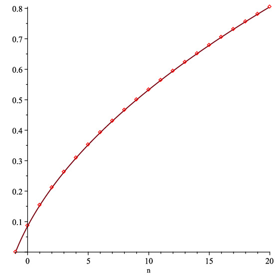
Figure 1: Numerical computation of $v_{n}$ (dots) with ${\epsilon}=0.1$, for $-1\leq n\leq 20$, compared with the graph of the approximation (1.12).

We define a set of non-negative sequences $\{\mathbf{b}^{(k)}\}_{k\geq 1}$ by successively applying $T$ to the zero sequence $\mathbf{0}$, so that

$$\mathbf{b}^{(-1)}=\mathbf{0},\qquad\mathbf{b}^{(k)}=T\mathbf{b}^{(k-1)}\quad\mathrm{for}\quad k\geq 0.$$ (2.2)

The first few steps in the $T$-orbit of $\mathbf{0}$ are specified by a formula for their terms, valid for all $n\geq 0$:

$$\mathrm{b}_{n}^{(0)}={\epsilon}(n+1),\qquad\mathrm{b}_{n}^{(1)}=\frac{{\epsilon}(n+1)}{1+2{\epsilon}(n+1)},\qquad\mathrm{b}_{n}^{(2)}=\frac{{\epsilon}(n+1)}{1+\frac{{\epsilon}n}{1+2{\epsilon}n}+\frac{{\epsilon}(n+2)}{1+2{\epsilon}(n+2)}}.$$ (2.3)

Thereafter, for $k\geq 3$, there is no longer a uniform expression for the iterate $\mathbf{b}^{(k)}$ as a ratio of polynomials

$$\mathrm{b}^{(k)}_{n}=\frac{\mathrm{p}_{n}^{(k)}({\epsilon})}{\mathrm{q}_{n}^{(k)}({\epsilon})}\qquad\mathrm{p}_{n}^{(k)},\mathrm{q}_{n}^{(k)}\in\mathbb{Z}[{\epsilon}],$$

valid for all $n$: due to the fact that the equations (2.1) defining $T$ for $n=0$ and $n>0$ are different, the coprime polynomials $\mathrm{p}_{n}^{(k)}({\epsilon}),\mathrm{q}_{n}^{(k)}({\epsilon})$ have distinct forms for $n=0,\ldots,k-3$, while there is another formula for them that is uniformly valid only for $n\geq k-2$. For instance, when $k=3$ we have

$$\mathrm{b}_{0}^{(3)}=\frac{{\epsilon}(1+12{\epsilon}+24{\epsilon}^{2})}{1+14{\epsilon}+40{\epsilon}^{2}+24{\epsilon}^{3}},\qquad\mathrm{and}\quad\mathrm{b}_{n}^{(3)}=\frac{\mathrm{p}_{n}^{(3)}({\epsilon})}{\mathrm{q}_{n}^{(3)}({\epsilon})}\quad\mathrm{for}\quad n\geq 1,$$

where

$$\mathrm{p}_{n}^{(3)}({\epsilon}) =(n+1){\epsilon}\Big{(}1+6n{\epsilon}+8(n^{2}-1){\epsilon}^{2}\Big{)}\Big{(}1+6(n+2){\epsilon}+8(n+1)(n+3){\epsilon}^{2}\Big{)},$$

$$\mathrm{q}_{n}^{(3)}({\epsilon}) =1+14(n+1){\epsilon}+8(9n^{2}+18n+4){\epsilon}^{2}+8(n+1)(21n^{2}+42n-11){\epsilon}^{3}$$

$$\qquad+16(n+1)^{2}(11n^{2}+22n-20){\epsilon}^{4}+64(n+1)^{3}(n-1)(n+3){\epsilon}^{5}.$$

Nevertheless, for all $n$ there are expressions for $\mathrm{b}^{(k)}_{n}$ as rational functions of $\epsilon$ and the variable $z={\epsilon}(n+1)$, which are described in Lemma 2.5 below.

If we start with a sequence $\mathbf{u}\in\mathcal{A}^{(0)}$ and apply $T$ once, then we find

$$\frac{{\epsilon}(n+1)}{1+{\epsilon}n+{\epsilon}(n+2)}\leq\frac{{\epsilon}(n+1)}{1+u_{n-1}+u_{n+1}}\leq{\epsilon}(n+1),$$

or in other words $\mathrm{b}_{n}^{(1)}\leq T(u_{n})\leq\mathrm{b}_{n}^{(0)}$, while another application of $T$ gives

$$\frac{{\epsilon}(n+1)}{1+{\epsilon}n+{\epsilon}(n+2)}\leq\frac{{\epsilon}(n+1)}{1+T(u_{n-1})+T(u_{n+1})}\leq\frac{{\epsilon}(n+1)}{\displaystyle 1+\frac{{\epsilon}n}{1+2{\epsilon}n}+\frac{{\epsilon}(n+2)}{1+2{\epsilon}(n+2)}},$$

so that $\mathrm{b}_{n}^{(1)}\leq T^{2}(u_{n})\leq\mathrm{b}_{n}^{(2)}$. Continuing in this way, by induction we obtain the following result.

Lemma 2.2.

For each non-negative integer $k$, the iterates $T^{k}\mathbf{u}$ of $\mathbf{u}\in\mathcal{A}^{(0)}$ satisfy the inequalities

$$\mathrm{b}_{n}^{(2j-1)}\leq T^{2j}(u_{n})\leq\mathrm{b}_{n}^{(2j)}\qquad\mathrm{for}\,\mathrm{all}\,n\geq 0,$$ (2.4)

when $k=2j$ is even, and

$$\mathrm{b}_{n}^{(2j+1)}\leq T^{2j+1}(u_{n})\leq\mathrm{b}_{n}^{(2j)}\qquad\mathrm{for}\,\mathrm{all}\,n\geq 0,$$ (2.5)

when $k=2j+1$ is odd. The sequences of lower/upper bounds in (2.2) satisfy

$$0\leq\mathrm{b}_{n}^{(2j-1)}<\mathrm{b}_{n}^{(2j+1)}<\mathrm{b}_{n}^{(2j+2)}<\mathrm{b}_{n}^{(2j)}\qquad\mathrm{for}\,\mathrm{all}\,n\geq 0,$$ (2.6)

for each $j\in\mathbb{N}$.

For each $k\geq 0$ we have the set $\mathcal{A}^{(k)}=T^{k}\mathcal{A}^{(0)}$, and the preceding result implies that the next set in the sequence, $\mathcal{A}^{(k+1)}\subset{A}^{(k)}$, is a proper subset of the previous one. Furthermore, the inequalities (2.6) immediately imply the existence of the limits of upper and lower bounds, that is

$$\lim_{j\to\infty}\mathrm{b}_{n}^{(2j-1)}=\limsup_{j\geq 0}\mathrm{b}_{n}^{(2j-1)}\leq\liminf_{j\geq 0}\mathrm{b}_{n}^{(2j)}=\lim_{j\to\infty}\mathrm{b}_{n}^{(2j)}$$ (2.7)

for each $n\geq 0$. The problem is then how to show the equality of the upper and lower limits above for each $n$, since in that case a squeezing argument immediately implies that the iterates $T^{k}\mathbf{u}$ converge to the unique positive fixed point of $T$.

Proposition 2.3.

For all ${\epsilon}>0$ there exists (at least one) $v_{0}=v_{0}({\epsilon})$ such that the solution of (1.13) with the initial data (1.14) is positive, and satisfies $v_{n}>0$ for all $n\geq 0$, as well as

$$\mathbf{v}=(v_{n})_{n\geq 0}\in\underset{k\geq 0}{\cap}{\cal A}^{(k)},$$

so that, for all $n\geq 0$,

$$\lim_{j\to\infty}\mathrm{b}_{n}^{(2j-1)}\leq v_{n}\leq\lim_{j\to\infty}\mathrm{b}_{n}^{(2j)}.$$ (2.8)

• The existence of a positive solution $\mathbf{v}$ is proved in [5], where it shown that for each ${\epsilon}>0$ there is an infinite sequence of open intervals $I_{k}=I_{k}({\epsilon})\subset\mathbb{R}$, with $I_{1}=(0,{\epsilon})$ and $I_{k}\subset I_{k-1}$, such that $v_{0}\in I_{k}\implies v_{1},\ldots,v_{k}>0$, and ${\cap}_{k\geq 0}\,{I_{k}}\neq\emptyset$. Hence if $v_{0}\in{\cap}_{k\geq 0}\,{I_{k}}$ then the corresponding sequence $\mathbf{v}$ is a positive solution. Then, because $T\mathbf{v}=\mathbf{v}$, it follows from Lemma 2.2 that $\mathbf{v}\in{\cal A}^{(k)}$ for each $k\geq 0$, and hence (2.8) holds for each $n\geq 0$. ∎

It is instructive to compare the upper and lower bounds for different $n$, as well as introducing the rescaled bounds $\rho_{n}^{(k)}$, which specify the norms:

$$\rho_{n}^{(k)}=\frac{\mathrm{b}_{n}^{(k)}}{{\epsilon}(n+1)},\qquad\|\mathbf{b}^{(k)}\|=\underset{n\geq 0}{\sup}\,\rho_{n}^{(k)}.$$

Clearly we have $\rho_{n}^{(-1)}=0$, while $\mathrm{b}_{n+1}^{(0)}>\mathrm{b}_{n}^{(0)}$ and $\rho_{n}^{(0)}=1$ for all $n$, and from (2.6) we also see that

$$0<\rho_{n}^{(k)}<1\qquad\mathrm{for}\,\mathrm{all}\,n\geq 0,k\geq 1.$$ (2.9)

If we now assume for some $k$ that $\mathrm{b}_{n+1}^{(k)}>\mathrm{b}_{n}^{(k)}$ holds for all $n\geq 0$, then from the definition of the map $T$ we may write

$$\frac{1}{\rho_{n+1}^{(k+1)}}-\frac{1}{\rho_{n}^{(k+1)}} =\big{(}1+\mathrm{b}_{n}^{(k)}+\mathrm{b}_{n+2}^{(k)}\big{)}-\big{(}1+\mathrm{b}_{n-1}^{(k)}+\mathrm{b}_{n+1}^{(k)}\big{)}$$

$$=\big{(}\mathrm{b}_{n}^{(k)}-\mathrm{b}_{n-1}^{(k)}\big{)}+\big{(}\mathrm{b}_{n+2}^{(k)}-\mathrm{b}_{n+1}^{(k)}\big{)}>0$$

where we set $\mathrm{b}_{-1}^{(k)}=0$ so that this makes sense when $n=0$, which implies that $\rho_{n+1}^{(k+1)}<\rho_{n}^{(k+1)}$. On the other hand,

$$\mathrm{b}_{n+1}^{(k)}>\mathrm{b}_{n}^{(k)}\iff(n+2)\rho_{n+1}^{(k)}>(n+1)\rho_{n}^{(k)},$$

and we can calculate

$$\frac{\mathrm{b}_{n+1}^{(k+1)}-\mathrm{b}_{n}^{(k+1)}}{\rho_{n+1}^{(k+1)}\rho_{n}^{(k+1)}} ={\epsilon}(n+2)\Big{(}1+\mathrm{b}_{n-1}^{(k)}+\mathrm{b}_{n+1}^{(k)}\Big{)}-{\epsilon}(n+1)\Big{(}1+\mathrm{b}_{n}^{(k)}+\mathrm{b}_{n+2}^{(k)}\Big{)}$$

$$={\epsilon}\Big{(}1+(n+2)\big{(}n\rho_{n-1}^{(k)}+(n+2)\rho_{n+1}^{(k)}\big{)}-(n+1)\big{(}(n+1)\rho_{n}^{(k)}+(n+3)\rho_{n+2}^{(k)}\big{)}\Big{)}.$$

If we now assume that $\rho_{n+1}^{(k)}<\rho_{n}^{(k)}$ holds for all $n\geq 0$, then we can replace the term with index $n+2$ above, and also (for $n>0$) replace the term with index $n-1$, and so rearrange to find the lower bound

$$\frac{\mathrm{b}_{n+1}^{(k+1)}-\mathrm{b}_{n}^{(k+1)}}{\rho_{n+1}^{(k+1)}\rho_{n}^{(k+1)}}>{\epsilon}\big{(}1+\rho_{n+1}^{(k)}-\rho_{n}^{(k)}\big{)}>0,$$

using (2.9) to obtain the final inequality. Thus, by induction on $k$, we find the following.

Lemma 2.4.

For $k\geq 0$, the sequences of lower/upper bounds satisfy

$$\mathrm{b}_{n+1}^{(k)}>\mathrm{b}_{n}^{(k)}\qquad\mathrm{for}\,\mathrm{all}\,n\geq 0,$$ (2.10)

while for $k\geq 1$ the rescaled bounds satisfy

$$\left(\frac{n+1}{n+2}\right)\,\rho_{n}^{(k)}<\rho_{n+1}^{(k)}<\rho_{n}^{(k)}\qquad\mathrm{for}\,\mathrm{all}\,n\geq 0,$$ (2.11)

and hence for each $k$ the norm of $\mathbf{b}^{(k)}$ is $\|\mathbf{b}^{(k)}\|=\rho_{0}^{(k)}$.

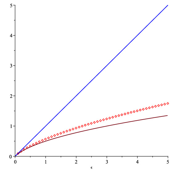
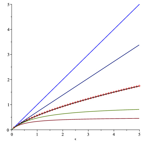
Figure 2: Left: numerical computation of $v_{0}({\epsilon})$ (dots) in the range $0<{\epsilon}\leq 5$, plotted against linear bound $b_{0}^{(0)}={\epsilon}$ and approximation $\mathrm{v}_{0}({\epsilon})$ as in (2.33). Right: same computation, but compared with upper bounds $b_{0}^{(0)},b_{0}^{(2)}$, lower bounds $b_{0}^{(1)},b_{0}^{(3)}$, and exact formula (1.16).

Lemma 2.5.

For each $j\geq 0$, the rescaled bounds have the asymptotic behaviour

$$\rho_{n}^{(2j)}\sim\frac{1}{j+1},\qquad\rho_{n}^{(2j+1)}\sim\frac{j+1}{2{\epsilon}(n+1)},\qquad\mathrm{as}\quad n\to\infty.$$ (2.12)

Moreover, the leading part of the Taylor expansion of each of the rescaled bounds at ${\epsilon}=0$ is

$$\rho_{n}^{(k)}=1-2{\epsilon}(n+1)+O({\epsilon}^{2})\qquad\mathrm{for}\,\mathrm{all}\,k\geq 1,$$ (2.13)

while for all ${\epsilon}>0$ the first derivatives with respect to ${\epsilon}$ satisfy

$$\frac{\mathrm{d}\rho_{n}^{(k)}}{\mathrm{d}{\epsilon}}<0,\qquad\frac{\mathrm{d}\mathrm{b}_{n}^{(k)}}{\mathrm{d}{\epsilon}}>0$$ (2.14)

for $k\geq 1$, $n\geq 0$, so that each bound $\rho_{n}^{(k)}$, $\mathrm{b}_{n}^{(k)}$ is monotone decreasing/increasing in ${\epsilon}$, respectively.

• As noted above, the action of the map $T$ is such that the components $\mathrm{b}_{n}^{(k)}$ of the sequences $\mathbf{b}^{(k)}$ are rational functions of ${\epsilon}$ which have an expression as ratios of coprime polynomials in ${\epsilon}$ that is uniformly valid for all $n$ when $k<3$, while for $k\geq 3$ these polynomials have a uniform structure for $n\geq k-2$ only. However, if we set $z={\epsilon}(n+1)$, then for $k=0,1,2$ we can write

  $$\rho_{n}^{(0)}=R^{(0)}(z,{\epsilon}):=1,\quad\rho_{n}^{(1)}=R^{(1)}(z,{\epsilon}):=\frac{1}{1+2z},\quad\rho_{n}^{(2)}=R^{(2)}(z,{\epsilon}):=\frac{1}{1+\frac{z-{\epsilon}}{1+2(z-{\epsilon})}+\frac{z+{\epsilon}}{1+2(z+{\epsilon})}},$$ (2.15)

  and for all $n$ we can similarly express $\rho_{n}^{(k)}$ as $R^{(k)}(z,{\epsilon})$, a rational function of $z$ and ${\epsilon}$ that is determined recursively via the finite difference equation

  $$R^{(k+1)}(z,{\epsilon})=\frac{1}{1+(z-{\epsilon})R^{(k)}(z-{\epsilon},{\epsilon})+(z+{\epsilon})R^{(k)}(z+{\epsilon},{\epsilon})}.$$ (2.16)

  So from the definition of the map $T$, the identity $\rho_{n}^{(k)}=R^{(k)}({\epsilon}(n+1),{\epsilon})$ holds for all $n$. The result (2.12) thus corresponds to the asymptotics of the rational functions $R^{(k)}(z,{\epsilon})$ as $z\to\infty$, which varies according to the parity of $k$, and we can proceed by induction on $j$. For the base case $j=0$ we have $R^{(0)}(z,{\epsilon})=1$, $R^{(1)}(z,{\epsilon})\sim\frac{1}{2z}$, so the claim for $\rho_{n}^{(0)}$ is trivially true, while for $\rho_{n}^{(1)}$ it gives the correct result by substituting $z={\epsilon}(n+1)$. So for the induction, for some fixed $j$ we can assume that $R^{(2j)}(z,{\epsilon})\sim\frac{1}{j+1}$ as $z\to\infty$, and then by applying (2.16) we immediately obtain

  $$R^{(2j+1)}(z,{\epsilon})\sim\left(1+\frac{z-{\epsilon}}{j+1}+\frac{z+{\epsilon}}{j+1}\right)^{-1}\sim\frac{j+1}{2z},\qquad z\to\infty,$$

  which, upon setting $z={\epsilon}(n+1)$ gives the correct leading order behaviour for $\rho_{n}^{(2j+1)}$ as $n\to\infty$. Applying (2.16) once again gives

  $$R^{(2j+2)}(z,{\epsilon})\sim\left(1+\frac{(z-{\epsilon})(j+1)}{2z}+\frac{(z+{\epsilon})(j+1)}{2z}\right)^{-1}\sim\frac{1}{j+2},\qquad z\to\infty,$$

  and this completes the inductive step.

  For the leading order behaviour of the scaled bounds at ${\epsilon}=0$, it is convenient to write an equivalent version of (2.16) in terms of $\rho_{n}^{(k)}$, namely

  $$\rho_{n}^{(k+1)}=\left(1+{\epsilon}n\rho_{n-1}^{(k)}+{\epsilon}(n+2)\rho_{n+1}^{(k)}\right)^{-1},$$ (2.17)

  which is valid for all $n$. When $k=1$, the leading order expansion (2.13) is immediately obtained from the geometric series for

  $$\rho_{n}^{(1)}=\frac{1}{1+2{\epsilon}(n+1)},$$ (2.18)

  and the general case easily follows via induction on $k$, by applying (2.17) at each step.

  To obtain the monotonicity in ${\epsilon}$ of $\rho_{n}^{(k)}$ and $\mathrm{b}_{n}^{(k)}$, it is clear from (2.18) and from $\mathrm{b}_{n}^{(1)}=\tfrac{1}{2}\big{(}1-\rho_{n}^{(1)}\big{)}$, that the inequalities (2.14) hold for $k=1$, and we proceed by induction on $k$. For convenience, we use a dot to denote the derivative with respect to ${\epsilon}$. Then, assuming that (for all $n\geq 0$) both $\dot{\rho}_{n}^{(k)}<0$ and $\dot{\mathrm{b}}_{n}^{(k)}>0$ hold from some $k$, differentiating (2.17) yields

  $$\dot{\rho}_{n}^{(k+1)}=-\big{(}\rho_{n}^{(k+1)}\big{)}^{2}\left(\dot{\mathrm{b}}_{n-1}^{(k)}+\dot{\mathrm{b}}_{n+1}^{(k)}\right)<0,$$ (2.19)

  implying that $\rho_{n}^{(k+1)}$ is monotone decreasing in ${\epsilon}$. Now differentiating $\mathrm{b}_{n}^{(k+1)}={\epsilon}(n+1)\rho_{n}^{(k+1)}$ yields

  $$\begin{array}[]{rcl}\dot{\mathrm{b}}_{n}^{(k+1)}&=&(n+1)\big{(}\rho_{n}^{(k+1)}+{\epsilon}\dot{\rho}_{n}^{(k+1)}\big{)}\\ &=&(n+1)\rho_{n}^{(k+1)}\Big{(}1-{\epsilon}\rho_{n}^{(k+1)}(\dot{\mathrm{b}}_{n-1}^{(k)}+\dot{\mathrm{b}}_{n+1}^{(k)})\Big{)}\\ &=&\mathrm{b}_{n}^{(k+1)}\Big{(}{\epsilon}^{-1}-\rho_{n}^{(k+1)}(\dot{\mathrm{b}}_{n-1}^{(k)}+\dot{\mathrm{b}}_{n+1}^{(k)})\Big{)},\end{array}$$

  where we used (2.19). Then we calculate

  $$\dot{\mathrm{b}}_{n-1}^{(k)}+\dot{\mathrm{b}}_{n+1}^{(k)}=n\big{(}\rho_{n-1}^{(k)}+{\epsilon}\dot{\rho}_{n-1}^{(k)}\big{)}+(n+2)\big{(}\rho_{n+1}^{(k)}+{\epsilon}\dot{\rho}_{n+1}^{(k)}\big{)}<n\rho_{n-1}^{(k)}+(n+2)\rho_{n+1}^{(k)}={\epsilon}^{-1}\big{(}\mathrm{b}_{n-1}^{(k)}+\mathrm{b}_{n+1}^{(k)}\big{)},$$

  using the inductive hypothesis on $\dot{\rho}_{n}^{(k)}$, and together with (2.17) this implies that

  $$\dot{\mathrm{b}}_{n}^{(k+1)}>\frac{\mathrm{b}_{n}^{(k+1)}}{{\epsilon}}\left(1-\rho_{n}^{(k+1)}\big{(}\mathrm{b}_{n-1}^{(k)}+\mathrm{b}_{n+1}^{(k)}\big{)}\right)=\frac{\mathrm{b}_{n}^{(k+1)}\rho_{n}^{(k+1)}}{{\epsilon}}>0,$$

  as required. ∎

Remark 2.6.

Since the sequence $(\rho_{n}^{(2j)})_{n\geq 0}$ decreases monotonically with $n$, as in Lemma 2.4, and tends to $1/(j+1)$, it follows that $\rho_{n}^{(2j)}>\frac{1}{j+1}$ for all $n\geq 0$, while the recursion (2.17) with $k=2j$ shows that $\rho_{n}^{(2j+1)}<\frac{j+1}{2{\epsilon}(n+1)}$, which is equivalent to $\mathrm{b}_{n}^{(2j+1)}<\frac{j+1}{2}$.

To further address our main assertion about the uniqueness of the positive solution of (1.13), we introduce the differences

$$\Delta^{(k)}_{n}=(-1)^{k}\big{(}\rho^{(k)}_{n}-\rho^{(k-1)}_{n}\big{)},$$ (2.20)

where the alternating sign is chosen so that $\Delta^{(k)}_{n}>0$ for all $k\geq 0$, $n\geq 0$, as is seen directly by dividing the inequalities (2.6) by ${\epsilon}(n+1)$ for each $n$. Then the coincidence of the lower and upper limits in (2.7), which yields the desired squeezing argument, is equivalent to the statement that

$$\lim_{k\to\infty}\Delta^{(k)}_{n}=0\qquad\mathrm{for}\,\mathrm{each}\,n\geq 0.$$ (2.21)

To see why the latter result is plausible, we consider the behaviour of these differences for small ${\epsilon}$, which will be needed later.

Lemma 2.7.

The leading part of the Taylor expansion of each of the differences (2.20) at ${\epsilon}=0$ is

$$\Delta^{(k)}_{n}=c_{n}^{(k)}\,{\epsilon}^{k}\Big{(}1+O({\epsilon})\Big{)},$$

where $c_{n}^{(0)}=1$ for all $n$, and the leading coefficient is given recursively by

$$c^{(k+1)}_{n}=nc^{(k)}_{n-1}+(n+2)c^{(k)}_{n+1}\qquad\mathrm{for}\,\,\mathrm{all}\,\,k,n\geq 0.$$ (2.22)

• The result is by induction on $k$. For the base case $k=0$ we have $\Delta^{(0)}_{n}=1$, and hence $c_{n}^{(0)}=1$, for all $n$. For the inductive step, we write

  $$\rho^{(k)}_{n}-\rho^{(k+1)}_{n}=\rho^{(k)}_{n}\rho^{(k+1)}_{n}\Big{(}(\rho^{(k+1)}_{n})^{-1}-(\rho^{(k)}_{n})^{-1}\Big{)},$$

  and so, by using (2.17) and collecting terms inside the round brackets, we obtain the identity

  $$\Delta^{(k+1)}_{n}=\rho^{(k)}_{n}\rho^{(k+1)}_{n}\big{(}{\epsilon}n\Delta^{(k)}_{n-1}+{\epsilon}(n+2)\Delta^{(k)}_{n+1}\big{)}.$$ (2.23)

  Upon using the inductive hypothesis and substituting in the leading order expansion (2.13) for the two prefactors on the right-hand side of (2.23), we immediately obtain $\Delta^{(k+1)}_{n}=c_{n}^{(k+1)}\,{\epsilon}^{k+1}\big{(}1+O({\epsilon})\big{)}$, where (for each $n$) the leading coefficient $c_{n}^{(k+1)}$ is given in terms of the coefficients with superscript $k$ by the recursion (2.22), as required. ∎

Note that we have $c_{n}^{(1)}=2(n+1)$, $c_{n}^{(2)}=4(n^{2}+2n+2)$, and it is apparent from (2.22) that these leading coefficients are monotone increasing with $n$, that is $c_{n+1}^{(k)}>c_{n}^{(k)}$, for $k\geq 1$. This monotonicity is desirable, since it suggests that, for small enough ${\epsilon}$, we should have $\Delta^{(k)}_{n+1}>\Delta^{(k)}_{n}$, while from Lemma 2.5 we see that

$$\lim_{n\to\infty}\Delta^{(2j)}_{n}=\frac{1}{j+1}=\lim_{n\to\infty}\Delta^{(2j+1)}_{n};$$ (2.24)

so if the sequence $(\Delta^{(k)}_{n})_{n\geq 0}$ is increasing with $n$ for each $k\geq 1$, then the sought after result (2.21) follows immediately from taking the limit $j\to\infty$ in (2.24). However, the monotonicity of $c_{n}^{(k)}$ in $n$ is not enough, because the convergence of the Taylor series (2.13), and hence the result of Lemma 2.7, does not hold uniformly in $n$. For instance, the geometric series for $\rho_{n}^{(1)}$ has radius of convergence $\tfrac{1}{2(n+1)}$. Moreover, if we introduce the functions

$$\Delta^{(k)}(z,{\epsilon})=(-1)^{k}\Big{(}R^{(k)}(z,{\epsilon})-R^{(k-1)}(z,{\epsilon})\Big{)}$$ (2.25)

in terms of the $R^{(k)}(z,{\epsilon})$ satisfying (2.16), then we might hope to use their behaviour in the range $z\geq{\epsilon}$ to determine suitable bounds on the discrete set of values $\Delta^{(k)}_{n}=\Delta^{(k)}\big{(}(n+1)\,{\epsilon},{\epsilon}\big{)}$. However, this turns out to be tricky for two reasons: first of all, we can show that $\Delta^{(2)}(z,{\epsilon})$ and the other functions (2.25) are not monotone in $z$ except for small ${\epsilon}\lesssim 0.3$; and secondly, for $k\geq 3$ these rational functions have poles at certain points in the range $z\geq{\epsilon}$, lying in between the discrete values of interest, so they are unbounded on this range. Figure 3 illustrates these features for $k=2$ and $4$.

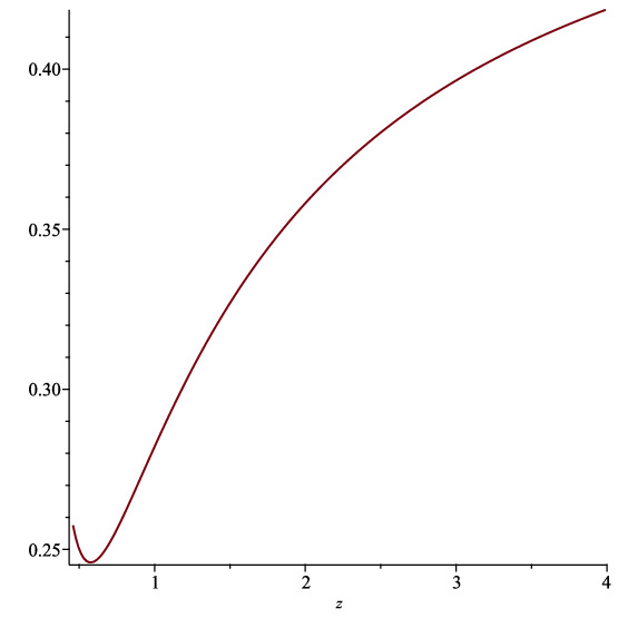
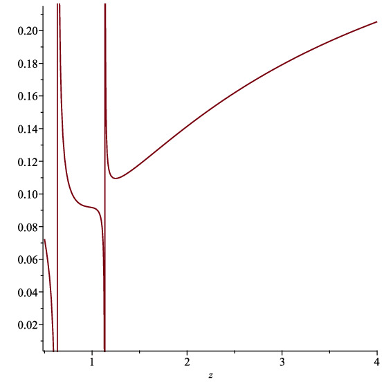
Figure 3: Left: graph of $\Delta^{(2)}(z,{\epsilon})$ against $z$ for ${\epsilon}=0.5$ showing the range $0.5\leq z\leq 4$, illustrating the local minimum in the interval ${\epsilon}<z<2{\epsilon}$. Right: graph of $\Delta^{(4)}(z,{\epsilon})$ against $z$ for ${\epsilon}=0.5$, showing vertical asymptotes at two poles, lying in the intervals ${\epsilon}<z<2{\epsilon}$ and $2{\epsilon}<z<3{\epsilon}$, respectively.

Further numerical investigations suggest that if ${\epsilon}$ is not two large, then the products $\rho_{n}^{(2j+1)}\rho_{n}^{(2j)}$ and $\rho_{n}^{(2j)}\rho_{n}^{(2j-1)}$ appear to be bounded above by their values as $n\to\infty$, as in (2.12). This is in spite of Remark 2.6, which shows that each product consists of an upper bound for one of the factor and a lower bound for the other. It is easy to see that $\rho_{n}^{(1)}\rho_{n}^{(0)}<\tfrac{1}{2{\epsilon}(n+1)}$, so the first case of interest is the product $\rho_{n}^{(2)}\rho_{n}^{(1)}$, for which the required bound can be expressed as $R^{(2)}(z,{\epsilon})R^{(1)}(z,{\epsilon})<\frac{1}{4z}$ for $z\geq{\epsilon}$, and this can be shown to be equivalent to the condition

$$\rho^{(2)}_{0}\rho^{(1)}_{0}=\frac{(1+4{\epsilon})}{(1+2{\epsilon})(1+6{\epsilon})}<\frac{1}{4{\epsilon}}$$

which is satisfied whenever $0<{\epsilon}<\frac{1}{2}(\sqrt{2}+1)$. This leads to the following

Conjecture 2.8.

For each value of ${\epsilon}$ in the range $0<{\epsilon}<{\epsilon}^{\star}$, where

$${\epsilon}^{*}=\frac{1}{2}(\sqrt{2}+1)\approx 1.2071,$$ (2.26)

the rescaled bounds satisfy

$$\rho_{n}^{(2j-1)}\rho_{n}^{(2j-2)}<\frac{1}{2{\epsilon}(n+1)}\qquad\mathrm{and}\qquad\rho_{n}^{(2j)}\rho_{n}^{(2j-1)}<\frac{j}{2{\epsilon}(n+1)(j+1)},$$ (2.27)

for all $n\geq 0$ and all $j\geq 1$.

The desirability of the bounds in (2.27), and especially the second one, comes from the fact that it immediately yields an inductive proof that

$$\Delta^{(2j+1)}_{n}<\Delta^{(2j)}_{n}<\frac{1}{j+1}\qquad\mathrm{for}\,\,n\geq 0$$ (2.28)

is valid for all $j\geq 1$. Indeed, the first inequality above is always true (from Lemma 2.2), while for the second one the inductive step is to use (2.23) to obtain

$$\begin{array}[]{rcl}\Delta^{(2j+2)}_{n}&=&\rho^{(2j+2)}_{n}\rho^{(2j+1)}_{n}\big{(}{\epsilon}n\Delta^{(2j+1)}_{n-1}+{\epsilon}(n+2)\Delta^{(2j+1)}_{n+1}\big{)}\\ &<&\frac{j+1}{2{\epsilon}(n+1)(j+2)}\left({\epsilon}n\big{(}\frac{1}{j+1}\big{)}+{\epsilon}(n+2)\big{(}\frac{1}{j+1}\big{)}\right)=\frac{1}{j+2},\end{array}$$

as required (where we used (2.27) and the inductive hypothesis to get the inequality). Taking $j\to\infty$ in (2.28), it then follows that $\lim_{j\to\infty}\Delta^{(2j)}_{n}=0=\lim_{j\to\infty}\Delta^{(2j+1)}_{n}$ for all $n\geq 0$, yielding the desired squeezing argument, and thus we have

Corollary 2.9.

If Conjecture 2.8 is valid, then there is a unique positive solution of (1.13) with initial data (1.14) whenever ${\epsilon}$ lies in the range (2.26).

We have tried in vain to provide a direct proof of Theorem 2.1, based only on the properties of the mapping $T$. The best we have so far is Corollary 2.9, which relies on an unproven assumption. Fortunately, all is not lost, because in the next section the connection between (1.13) and the space of initial conditions for Painlevé V will be made manifest. Consequently, this will lead to identifying the initial value problem (1.14) with certain classical solutions of Painlevé V, and resulting not only in a proof that the positive solution is unique, but also in an explicit formula for this solution.

Before switching gears and moving on to consider the geometry of (1.13), we present one more technical result concerning positive solutions.

Proposition 2.10.

For each $k\geq 0$, any positive solution of (1.13) satisfies

$$v_{n}=\sum_{i=0}^{k}(-1)^{i}s_{n,i}\,{\epsilon}^{i+1}+O({\epsilon}^{k+2})\qquad\mathrm{as}\,\,{\epsilon}\to 0,$$ (2.29)

where the finite sum coincides with the first $k+1$ non-zero terms in the Taylor expansion of the rational function $\mathrm{b}_{n}^{(k)}$ at ${\epsilon}=0$, that is

$$\mathrm{b}_{n}^{(k)}({\epsilon})=\sum_{i=0}^{k}(-1)^{i}s_{n,i}\,{\epsilon}^{i+1}+O({\epsilon}^{k+2}),$$ (2.30)

where the coefficients $s_{n,i}$ depend only on $n$. In particular, for all $n\geq 0$, $s_{n,0}=n+1$, $s_{n,1}=2(n+1)^{2}$, $s_{n,2}=8(n+1)^{3}+4(n+1)$, independent of $k$.

• By Lemma 2.7, for all $k\geq 0$ and for each $n\geq 0$ the Taylor expansions of $\rho_{n}^{(k)}$ and $\rho_{n}^{(k+1)}$ at ${\epsilon}=0$ agree up to and including terms of order ${\epsilon}^{k}$, which implies that the corresponding Taylor expansions of $\mathrm{b}_{n}^{(k)}$ and $\mathrm{b}_{n}^{(k+1)}$ agree as far as order ${\epsilon}^{k+1}$, with their first $k+1$ non-zero terms depending only on $n$, as in (2.30). Then by Proposition 2.3, together the bounds in Lemma 2.2, a positive solution must satisfy

  $$v_{n}-\sum_{i=0}^{k}(-1)^{i}s_{n,i}\,{\epsilon}^{i+1}=O({\epsilon}^{k+2})\qquad\mathrm{as}\,\,{\epsilon}\to 0,$$

  for each $k$. From (2.13) it follows that

  $$\mathrm{b}_{n}^{(k)}=(n+1){\epsilon}\,\big{(}1-2(n+1){\epsilon}+O({\epsilon}^{2})\big{)}$$

  for $k\geq 1$, giving the stated expressions for $s_{n,0}$ and $s_{n,1}$, while $s_{n,2}$ is obtained from expanding $\mathrm{b}_{n}^{(k)}$ in (2.3) up to $O({\epsilon}^{3})$; but for $k\geq 3$ these coefficients do not have a uniform expression in $n$. ∎

The expansions (2.29) extend to an asymptotic series

$$v_{n}\sim\sum_{i=0}^{\infty}(-1)^{i}s_{n,i}\,{\epsilon}^{i+1}$$ (2.31)

for each $n$. In particular, when $n=0$ the series is

$$v_{0}\sim{\epsilon}-2{\epsilon}^{2}+12{\epsilon}^{3}-112{\epsilon}^{4}+1392{\epsilon}^{5}-21472{\epsilon}^{6}+\ldots\qquad\mathrm{as}\quad{\epsilon}\to 0.$$ (2.32)

This should be compared with the Taylor expansion at ${\epsilon}=0$ of (1.12) when $n=0$, that is

$$\mathrm{v}_{0}({\epsilon})=\tfrac{1}{4}\left(\sqrt{1+8{\epsilon}}-1\right)={\epsilon}-2{\epsilon}^{2}+8{\epsilon}^{3}-40{\epsilon}^{4}+\ldots.$$ (2.33)

The bounds $\mathrm{b}_{n}^{(k)}$ provide a sequence of rational approximations which alternate between upper/lower bounds for even/odd $k$. This is highly reminiscent of the situation for the convergents of Stieltjes-type continued fractions (S-fractions), which also provide successive upper/lower approximations based on a formal series. Indeed, such a fraction can be associated with the series (2.31), which from the stated expressions for $s_{n,0}$, $s_{n,1}$ and $s_{n,2}$ must begin as follows:

$$v_{n}=\cfrac{(n+1){\epsilon}}{1+\cfrac{2(n+1){\epsilon}}{1+\cfrac{2\Big{(}n+1+(n+1)^{-1}\Big{)}{\epsilon}}{1+\cdots}}}\,\,,$$ (2.34)

The corresponding continued fraction for $v_{0}$ has the form

$$v_{0}=\frac{{\epsilon}}{1+v_{1}}=\cfrac{{\epsilon}}{1+\cfrac{2{\epsilon}}{1+\cfrac{4{\epsilon}}{1+\cfrac{5{\epsilon}}{1+\cfrac{7{\epsilon}}{1+\cdots}}}}}\,\,,$$ (2.35)

whose coefficients will be described explicitly in due course, towards the end of section 4.

In fact, the continued fraction (2.35) will turn out to provide us with the missing step in the proof of uniqueness of the positive solution. Furthermore, for each ${\epsilon}>0$ it will precisely identify this solution as being the one specified by the initial condition

$$v_{0}=\tfrac{1}{2}\left(\frac{K_{5/6}(\tfrac{1}{2}t)}{K_{1/6}(\tfrac{1}{2}t)}-1\right),\qquad\mathrm{where}\quad t=\frac{1}{3{\epsilon}},$$

The latter function is plotted against ${\epsilon}$ in the panel on the right-hand side of Fig.2, with a set of numerical computations using the iterated map $T$ appearing as dots on top of this curve. A key feature of our analysis will be to use the fact that this function $v_{0}$ satisfies the Riccati equation

$$3{\epsilon}^{2}\frac{\mathrm{d}v_{0}}{\mathrm{d}{\epsilon}}={\epsilon}(1+2v_{0})-v_{0}-v_{0}^{2},$$ (2.36)

which gives a rapid way to generate the expansion (2.32) recursively, and similarly $v_{1}$ satisfies

$$3{\epsilon}^{2}\frac{\mathrm{d}v_{1}}{\mathrm{d}{\epsilon}}={\epsilon}(2+v_{1})-v_{1}-v_{1}^{2}.$$ (2.37)

These Riccati equations arise as special reductions of the Painlevé V equation, which we proceed to extract from the geometry of the discrete equation (1.13) in the next section.

3 Complex geometry of the dP_I equation

In this section, we obtain the space of initial conditions for the dP_I equation, and show that it corresponds to a particular case of the surface type $D_{5}^{(1)}$, with symmetry type $A_{3}^{(1)}$, coinciding with that for the Painlevé V equation.

Our goal is to describe the geometry of the equation (1.13), and then use it to study some of its special solutions. This equation is a special case of the more general dP_I equation

$$x_{n+1}+x_{n-1}=\frac{\tilde{{\alpha}}n+\tilde{\beta}}{x_{n}}+\tilde{\gamma}$$ (3.1)

for $\tilde{{\alpha}}=\tilde{\beta}={\epsilon}$ and $\tilde{\gamma}=-1$, so we do the general case and then specialise. This equation has been studied in [13, 14, 15, 26, 30]; see also [20].

We first construct the family of Sakai surfaces regularizing the dynamics (3.1). For that, we begin by rewriting the recurrence as a first-order discrete dynamical system on $\mathbb{C}^{1}\times\mathbb{C}^{1}$ via $y_{n}:=x_{n+1}$. Then equation (3.1) can be rewritten as $y_{n}+x_{n-1}=(\tilde{{\alpha}}n+\tilde{\beta})/x_{n}+\tilde{\gamma}$ and we get the mapping

$$\varphi_{n}(x_{n},y_{n})=\left(y_{n},\frac{\tilde{{\alpha}}(n+1)+\tilde{\beta}}{y_{n}}+\tilde{\gamma}-x_{n}\right).$$ (3.2)

Using the notation $\overline{x}_{n}=x_{n+1}$, $\underline{x}_{n}=x_{n-1}$, and same for $y_{n}$, we can omit the indices and rewrite our mapping and its inverse as

$$\varphi(x,y)=\left(y,\frac{\tilde{{\alpha}}(n+1)+\tilde{\beta}}{y}+\tilde{\gamma}-x\right),\qquad\varphi^{-1}(x,y)=\left(\frac{\tilde{{\alpha}}n+\tilde{\beta}}{y}+\tilde{\gamma}-y,x\right).$$ (3.3)

Next, we extend the mapping to $\mathbb{P}^{1}\times\mathbb{P}^{1}$ via the introducion of coordinates at infinity, $X=1/x$ and $Y=1/y$, and then rewrite the mappings (3.3) from the affine chart $(x,y)$ to three other charts, $(X,y)$, $(x,Y)$, and $(X,Y)$. It is easy to see that there are four base points where either rational mapping becomes undefined, which are

$$\left(X=0,y=0\right),\quad(X=0,y=\tilde{\gamma}),\quad(x=0,Y=0),\quad(x=\tilde{\gamma},Y=0).$$ (3.4)

As usual, these singularities are resolved by using blowups, where blowing up a point $q_{i}(x_{i},y_{i})$ amounts to introducing two new coordinate charts $(\mathrm{u}_{i},\mathrm{v}_{i})$ and $(U_{i},V_{i})$ via $x=x_{i}+\mathrm{u}_{i}=x_{i}+U_{i}V_{i}$ and $y=y_{i}+\mathrm{u}_{i}\mathrm{v}_{i}=y_{i}+V_{i}$. We then extend the mapping to these new charts, check for new base points, resolve them in the same way, and continue this process until the mapping becomes defined everywhere. This process, for discrete Painlevé equations, terminates in a finite number of steps, and in our case, as usual, we get $8$ base points that come in four degeneration cascades,

$$q_{1}\left(X=\frac{1}{x}=0,y=\tilde{\gamma}\right) \leftarrow q_{2}\left(\mathrm{u}_{1}=X=\frac{1}{x}=0,\mathrm{v}_{1}=x(y-\tilde{\gamma})=\tilde{{\alpha}}\right),$$ (3.5)

$$q_{3}\left(X=\frac{1}{x}=0,y=0\right) \leftarrow q_{4}\left(\mathrm{u}_{3}=X=\frac{1}{x}=0,\mathrm{v}_{3}=xy=(n+1)\tilde{{\alpha}}+\tilde{\beta}\right),$$

$$q_{5}\left(x=0,Y=\frac{1}{y}=0\right) \leftarrow q_{6}\left(U_{5}=xy=n\tilde{{\alpha}}+\tilde{\beta},V_{5}=Y=\frac{1}{y}=0\right),$$

$$q_{7}\left(x=\tilde{\gamma},Y=\frac{1}{y}=0\right) \leftarrow q_{8}\left(U_{7}=y(x-\tilde{\gamma})=-\tilde{{\alpha}},V_{7}=Y=\frac{1}{y}=0\right).$$

This point configuration is easily identified as a point configuration for the $D_{5}^{(1)}$ Sakai surface family. This family can also be thought of as the Okamoto space of initial conditions for the differential equation $\text{P}_{\mathrm{V}}$, that is

$$\frac{\mathrm{d}^{2}{w}}{{\mathrm{d}{t}}^{2}}=\left(\frac{1}{2w}+\frac{1}{w-1}\right)\left(\frac{\mathrm{d}{w}}{{\mathrm{d}{t}}}\right)^{2}-\frac{1}{t}\frac{\mathrm{d}{w}}{{\mathrm{d}{t}}}+\frac{(w-1)^{2}}{t^{2}}\left({{\alpha}}w+\frac{{{\beta}}}{w}\right)+\frac{{{\gamma}}}{t}w+{\delta}\frac{w(w+1)}{w-1},$$ (3.6)

where ${\alpha},{\beta},{\gamma},{\delta}\in\mathbb{C}$ are complex parameters. From the point of view of geometry it is convenient to consider the Hamiltonian version of this equation in the form given in [20], namely

$$\left\{\begin{aligned} \frac{\mathrm{d}{q}}{{\mathrm{d}{t}}}&=\frac{1}{t}\Big{(}q(q-1)(2p+t)-a_{1}(q-1)-a_{3}q\Big{)}=\frac{\partial H}{\partial p},\\ \frac{\mathrm{d}{p}}{{\mathrm{d}{t}}}&=\frac{1}{t}\Big{(}p(p+t)(1-2q)+(a_{1}+a_{3})p-a_{2}t\Big{)}=-\frac{\partial H}{\partial q},\end{aligned}\right.$$ (3.7)

where the Hamiltonian function is

$$H(q,p;t)=\frac{1}{t}\Big{(}q(q-1)p(p+t)-(a_{1}+a_{3})qp+a_{1}p+a_{2}tq\Big{)},$$ (3.8)

and the symplectic form is the usual one, $\omega=\mathrm{d}p\wedge\mathrm{d}q$. The parameters $a_{i}$ are the so-called root variables that are related to the standard Painlevé parameters via

$${{\alpha}}=\tfrac{1}{2}{a_{1}^{2}},\quad{{\beta}}=-\tfrac{1}{2}{a_{3}^{2}},\quad{{\gamma}}=a_{0}-a_{2},\quad{\delta}=-\tfrac{1}{2},\qquad\text{where }\quad a_{0}+a_{1}+a_{2}+a_{3}=1.$$ (3.9)

The system (3.7) is equivalent to (3.6) for the function $w(t)=1-{1}/{p(t)}$. The Okamoto space of initial conditions for this system is obtained by removing the irreducible components of the anti-canonical divisor (the so-called vertical leaves) from the standard realization of the $D_{5}^{(1)}$-surface family. This family

$$\mathcal{X}=\mathcal{X}_{\mathbf{a}=(a_{0},a_{1},a_{2},a_{3})}=\operatorname{Bl}_{p_{1},\ldots,p_{n}}\left(\mathbb{P}^{1}\times\mathbb{P}^{1}\right),$$

is obtained by blowing up $\mathbb{P}^{1}\times\mathbb{P}^{1}$ at the points

$$p_{1}(\infty,-t)\leftarrow p_{2}(0,-a_{0}),\quad p_{3}(\infty,0)\leftarrow p_{4}(0,-a_{2}),\quad p_{5}(0,\infty)\leftarrow p_{6}(a_{1},0),\quad p_{7}(1,\infty)\leftarrow p_{8}(a_{3},0).$$ (3.10)

The latter point configuration and the resulting blowup surface are shown on Figure 4.

Figure 4: The standard $D_{5}^{(1)}$ Sakai surface family (the space of initial conditions for system (3.7))

Note that configurations (3.5) and (3.10) almost match — geometrically they are the same up to the action of rescaling on the axes. Thus, let $p=\lambda x$ and $q=\mu y$. Then the symplectic form is $\omega=\mathrm{d}p\wedge\mathrm{d}q=\lambda\mu\mathrm{d}x\wedge\mathrm{d}y$ and matching coordinates of the base points results in

$$\mu\tilde{\gamma}=-t,\quad\lambda\mu\tilde{{\alpha}}=-a_{0},\quad\lambda\mu(n\tilde{{\alpha}}+\tilde{\beta})=a_{1},\quad\lambda\mu((n+1)\tilde{{\alpha}}+\tilde{\beta})=-a_{2},\lambda\tilde{\gamma}=1,\quad\lambda\mu(-\tilde{{\alpha}})=a_{3}.$$

Thus, $\lambda=\tilde{\gamma}^{-1}$ and the root variable normalization $a_{0}+a_{1}+a_{2}+a_{3}=-3\tilde{{\alpha}}\lambda\mu=1$ gives $\mu=-\tilde{\gamma}(3\tilde{{\alpha}})^{-1}$. The root variables describing configurations (3.5) then are

$$a_{0}=\frac{1}{3},\quad a_{1}=-\frac{n}{3}-\frac{\tilde{\beta}}{3\tilde{{\alpha}}},\quad a_{2}=\frac{n+1}{3}+\frac{\tilde{\beta}}{3\tilde{{\alpha}}},\quad a_{3}=\frac{1}{3}.$$ (3.11)

In particular, we see that we get an integer translation in the root variables only after three iterations. This can also be seen directly by computing the push-forward $\varphi_{*}$ and the pull-back $\varphi^{*}=(\varphi_{*})^{-1}$ actions of the mapping (3.3) on the Picard lattice $\operatorname{Pic}(\mathcal{X})$. Specifying the basis as

$$\operatorname{Pic}(\mathcal{X})=\operatorname{Span}_{\mathbb{Z}}\{\mathcal{H}_{x},\mathcal{H}_{y},\mathcal{E}_{1},\ldots,\mathcal{E}_{8}\},$$ (3.12)

the corresponding actions of $\varphi_{*}$ and $\varphi^{*}$ are given by

$$\mathcal{H}_{y} \overset{\varphi^{*}}{\longleftarrow} \mathcal{H}_{x} \overset{\varphi_{*}}{\longrightarrow}\mathcal{H}_{x}+\mathcal{H}_{y}-\mathcal{E}_{5}-\mathcal{E}_{6},$$ (3.13)

$$\mathcal{H}_{x}+\mathcal{H}_{y}-\mathcal{E}_{3}-\mathcal{E}_{4} \longleftarrow \mathcal{H}_{y} \longrightarrow\mathcal{H}_{x},$$

$$\mathcal{E}_{5} \longleftarrow \mathcal{E}_{1} \longrightarrow\mathcal{E}_{7},$$

$$\mathcal{E}_{6} \longleftarrow \mathcal{E}_{2} \longrightarrow\mathcal{E}_{8},$$

$$\mathcal{E}_{7} \longleftarrow \mathcal{E}_{3} \longrightarrow\mathcal{H}_{x}-\mathcal{E}_{6},$$

$$\mathcal{E}_{8} \longleftarrow \mathcal{E}_{4} \longrightarrow\mathcal{H}_{x}-\mathcal{E}_{5},$$

$$\mathcal{H}_{y}-\mathcal{E}_{4} \longleftarrow \mathcal{E}_{5} \longrightarrow\mathcal{E}_{1},$$

$$\mathcal{H}_{y}-\mathcal{E}_{3} \longleftarrow \mathcal{E}_{6} \longrightarrow\mathcal{E}_{2},$$

$$\mathcal{E}_{1} \longleftarrow \mathcal{E}_{7} \longrightarrow\mathcal{E}_{3},$$

$$\mathcal{E}_{2} \longleftarrow \mathcal{E}_{8} \longrightarrow\mathcal{E}_{4}.$$

We initially use the same choice as in [20] for the surface root basis, shown on Figure 5, and the symmetry root bases, shown on Figure 6.

$$\raisebox{-32.1pt}{ \leavevmode\hbox to122.6pt{\vbox to72.32pt{\text{[drawing]}}}}\qquad\begin{aligned} \delta_{0}&=\mathcal{E}_{1}-\mathcal{E}_{2},&\qquad\delta_{3}&=\mathcal{H}_{p}-\mathcal{E}_{5}-\mathcal{E}_{7},\\ \delta_{1}&=\mathcal{E}_{3}-\mathcal{E}_{4},&\qquad\delta_{4}&=\mathcal{E}_{5}-\mathcal{E}_{6},\\ \delta_{2}&=\mathcal{H}_{q}-\mathcal{E}_{1}-\mathcal{E}_{3},&\qquad\delta_{5}&=\mathcal{E}_{7}-\mathcal{E}_{8}.\end{aligned} \delta_{0} \delta_{1} \delta_{2} \delta_{3} \delta_{4} \delta_{5}$$ (3.14)

Figure 5: The surface root basis for the standard $D_{5}^{(1)}$ Sakai surface point configuration

$$\raisebox{-32.1pt}{ \leavevmode\hbox to96.1pt{\vbox to69.68pt{\text{[drawing]}}}}\qquad\begin{aligned} {\alpha}_{0}&=\mathcal{H}_{p}-\mathcal{E}_{1}-\mathcal{E}_{2},&\qquad{\alpha}_{2}&=\mathcal{H}_{p}-\mathcal{E}_{3}-\mathcal{E}_{4},\\ {\alpha}_{1}&=\mathcal{H}_{q}-\mathcal{E}_{5}-\mathcal{E}_{6},&\qquad{\alpha}_{3}&=\mathcal{H}_{q}-\mathcal{E}_{7}-\mathcal{E}_{8}.\\[5.0pt] \hat{\delta}&=\mathrlap{{\alpha}_{0}+{\alpha}_{1}+{\alpha}_{2}+{\alpha}_{3}.}\end{aligned} {\alpha}_{0} {\alpha}_{1} {\alpha}_{2} {\alpha}_{3}$$ (3.15)

Figure 6: The symmetry root basis for the standard $A_{3}^{(1)}$ symmetry sub-lattice

Then the action of the mapping $\varphi_{*}$ on the symmetry roots is

$$\varphi_{*}:\upalpha=\langle{\alpha}_{0},{\alpha}_{1},{\alpha}_{2},{\alpha}_{3}\rangle\mapsto\langle{\alpha}_{3},{\alpha}_{0}+{\alpha}_{1},-{\alpha}_{1},{\alpha}_{1}+{\alpha}_{2}\rangle,$$ (3.16)

which is not a translation on the symmetry sub-lattice. However, it is a quasi-translation, since after three iterations we get a translation, that is

$$\varphi_{*}^{3}:\upalpha=\langle{\alpha}_{0},{\alpha}_{1},{\alpha}_{2},{\alpha}_{3}\rangle\mapsto\upalpha+\langle 0,1,-1,0\rangle\hat{\delta},\qquad\hat{\delta}=-\mathcal{K}_{\mathcal{X}}={\alpha}_{0}+{\alpha}_{1}+{\alpha}_{2}+{\alpha}_{3}.$$ (3.17)

There are two standard and non-conjugated examples of discrete Painlevé equations in the $D_{5}^{(1)}$-family: the equation given in [20, (8.23)], which acts on the symmetry roots as a translation

$$\psi_{*}:\upalpha=\langle{\alpha}_{0},{\alpha}_{1},{\alpha}_{2},{\alpha}_{3}\rangle\mapsto\upalpha+\langle-1,1,-1,1\rangle\,\hat{\delta};$$ (3.18)

and the equation in [28, (2.33-2.34)] that acts on the symmetry roots as a translation

$$\phi_{*}:\upalpha=\langle{\alpha}_{0},{\alpha}_{1},{\alpha}_{2},{\alpha}_{3}\rangle\mapsto\upalpha+\langle-1,0,0,1\rangle\,\hat{\delta}.$$ (3.19)

We see that the cube of our mapping is conjugated, by the half-turn rotation of the Dynkin diagrams, to the dynamics considered by Sakai, also called the dP_IV equation in the original Sakai paper [27].

Note that parameters ${{\alpha}},{{\beta}},{{\gamma}},{\delta}\in\mathbb{C}$ appearing as coefficients in the Painlevé V equation are

$${{\alpha}}=\frac{(n\tilde{{\alpha}}+\tilde{\beta})^{2}}{18\tilde{{\alpha}}^{2}},\quad{{\beta}}=-\frac{1}{18},\quad{{\gamma}}=-\frac{n\tilde{{\alpha}}+\tilde{\beta}}{3\tilde{{\alpha}}},\quad\delta=-\frac{1}{2},$$ (3.20)

and further specializing to equation (1.13) by taking $\tilde{{\alpha}}=\tilde{\beta}={\epsilon}$ and $\tilde{\gamma}=-1$ gives ${\lambda}=-1$, $\mu=1/(3{\epsilon})$ and

$$a_{0}=a_{3}=\frac{1}{3},\quad a_{1}=-\frac{n+1}{3},\quad a_{2}=\frac{n+2}{3};\qquad{{\alpha}}=\frac{(n+1)^{2}}{18},\quad{{\beta}}=-\frac{1}{18},\quad{{\gamma}}=-\frac{n+1}{3},$$ (3.21)

where the solution $w$ of (3.6) is related to the iterate $v_{n}$ of (1.13) via

$$w(t)=1+\frac{1}{v_{n}({\epsilon})}\qquad\mathrm{with}\quad t=\frac{1}{3{\epsilon}}.$$ (3.22)

An essential observation to make at this stage is that these values of the root variables, and the corresponding values of ${\alpha},{\beta},{\gamma}$, fall in a particular region of parameter space where the equation (3.6) is known to admit special solutions in terms of classical special functions: see [24, §32.10(v)], for instance. The subject of these classical solutions is what we now consider.

4 Classical solutions of dP_I from BTs for Painlevé V

In this section we present a large family of special solutions for the Painlevé V equation, connected to one another by Bäcklund transformations (BTs), and show how this includes a one-parameter family of solutions for (1.13), corresponding to an explicit orbit of the dynamics whose geometry was revealed in the preceding section. In the first subsection below, we will construct explicit Wronskian determinant formulae for these solutions, thus providing special solutions of $\tau$-function relations that were obtained in [5]. Finally, in the second subsection, we will complete the proof of uniqueness of the positive solution of (1.13), as well as proving Theorem 1.1.

We consider the generic case of P_V (1.15) when ${\delta}\not=0$, and as usual we set ${\delta}=-\tfrac{1}{2}$, i.e. we take

$$\frac{\mathrm{d}^{2}{y}}{{\mathrm{d}{t}}^{2}}=\left(\frac{1}{2y}+\frac{1}{y-1}\right)\left(\frac{\mathrm{d}{y}}{{\mathrm{d}{t}}}\right)^{\!\!2}-\frac{1}{t}\frac{\mathrm{d}{y}}{{\mathrm{d}{t}}}+\frac{(y-1)^{2}({\alpha}y^{2}+{\beta})}{t^{2}y}+\frac{{\gamma}y}{t}-\frac{y(y+1)}{2(y-1)}.$$ (4.1)

Suppose that $y$ satisfies P_V (4.1) with parameters $({\alpha},{\beta},{\gamma})=\big{(}\tfrac{1}{2}a^{2},-\tfrac{1}{2}b^{2},c\big{)}$; then the Bäcklund transformation $\mathcal{T}_{\varepsilon_{1},\varepsilon_{2},\varepsilon_{3}}$ is defined by

$$\mathcal{T}_{\varepsilon_{1},\varepsilon_{2},\varepsilon_{3}}(y) =1-\frac{2\varepsilon_{1}ty}{\displaystyle t\displaystyle\frac{\mathrm{d}{y}}{{\mathrm{d}{t}}}-\varepsilon_{2}ay^{2}+(\varepsilon_{2}a-\varepsilon_{3}b+\varepsilon_{1}t)y+\varepsilon_{3}b},$$ (4.2)

with $\varepsilon_{j}=\pm 1$, $j=1,2,3$, independently, and for the parameters

$$\mathcal{T}_{\varepsilon_{1},\varepsilon_{2},\varepsilon_{3}}\big{(}a,b,c\big{)}=\left(\tfrac{1}{2}\big{(}c+\varepsilon_{1}(1-\varepsilon_{3}b-\varepsilon_{2}a)\big{)},\tfrac{1}{2}\big{(}c-\varepsilon_{1}(1-\varepsilon_{3}b-\varepsilon_{2}a)\big{)},\varepsilon_{1}(\varepsilon_{3}b-\varepsilon_{2}a)\right),$$ (4.3)

see, for example, [16], [17, §39] or [24, §32.7(v)]. Note that the Bäcklund transformation $\mathcal{T}_{\varepsilon_{1},\varepsilon_{2},\varepsilon_{3}}$ is usually given for the parameters ${\alpha}$, ${\beta}$ and ${\gamma}$, in terms of $a$, $b$ and $c$. However in order to apply a sequence of Bäcklund transformations, it is better to define the effect of Bäcklund transformation on the parameters $a$, $b$ and $c$ to avoid any ambiguity in taking a square root. Indeed, the discrete symmetries of Painlevé V, corresponding to the extended affine Weyl group of type $A_{3}^{(1)}$, act naturally on the root variables, as in (3.9), and (up to fixing some choices of sign) the parameters $a,b,c$ here correspond to $a_{1},a_{3},a_{0}-a_{2}$ in the notation of the previous section.

To derive a discrete equation from Bäcklund transformations of a Painlevé equation, we use a Bäcklund transformation $\mathcal{R}$, which relates a solution $y$ to another solution $y_{+}$ and its inverse $\mathcal{R}^{-1}$, which relates $y$ to a third solution $y_{-}$. Then eliminating the derivative between the two Bäcklund transformations gives an algebraic equation relating $y$, $y_{+}$ and $y_{-}$, which is the discrete equation, cf. [7] for more details of this procedure, see also [11].

Consider the Bäcklund transformation $\mathcal{R}=\mathcal{T}_{-1,1,1}$ which has an inverse $\mathcal{R}^{-1}=\mathcal{T}_{-1,1,-1}\circ\mathcal{T}_{1,-1,-1}\circ\mathcal{T}_{1,-1,1}$, then

$$y_{+} =\mathcal{R}(y;a,b,c)=1+\frac{2ty}{\displaystyle t\displaystyle\frac{\mathrm{d}{y}}{{\mathrm{d}{t}}}-ay^{2}+(a-b-t)y+b},$$ (4.4a)

$$y_{-} =\mathcal{R}^{-1}(y;a,b,c)=1-\frac{2ty}{\displaystyle t\displaystyle\frac{\mathrm{d}{y}}{{\mathrm{d}{t}}}+ay^{2}-(a+b-t)y+b},$$ (4.4b)

and

$$(a_{+},b_{+},c_{+}) =\mathcal{R}(a,b,c)=\left(\tfrac{1}{2}\big{(}a+b+c-1\big{)},-\tfrac{1}{2}\big{(}a+b-c-1\big{)},a-b\right),$$

$$(a_{-},b_{-},c_{-}) =\mathcal{R}^{-1}(a,b,c)=\left(\tfrac{1}{2}\big{(}a-b+c+1\big{)},\tfrac{1}{2}\big{(}a-b-c+1\big{)},a+b\right).$$

Eliminating $\displaystyle\displaystyle\frac{\mathrm{d}{y}}{{\mathrm{d}{t}}}$ in (4.4) gives the algebraic equation relating $y$, $y_{+}$ and $y_{-}$, and comparing this with (3.22) with $w\to y$ we set $y=1+1/v$ and $y_{\pm}=1+1/v_{\pm}$, which gives

$$\frac{1}{y_{+}-1}+\frac{1}{y_{-}-1}=-\frac{a(y-1)}{t}-1\implies v_{+}+v_{-}=-1-\frac{a}{tv}.$$

Remark 4.1.

In terms of $y$, the transformation (4.4b) is the same as $\mathcal{T}_{1,-1,1}(y)$. However, the parameters $(a,b,c)$ map differently since

$$\mathcal{T}_{1,-1,1}(a,b,c)=\big{(}\tfrac{1}{2}(a-b+c-1),\tfrac{1}{2}(-a+b+c-1),a+b\big{)}.$$

Consequently it is straightforward to show that $\mathcal{T}_{1,-1,1}\circ\mathcal{T}_{-1,1,1}(y)=y$, but $\mathcal{T}_{-1,1,1}\circ\mathcal{T}_{1,-1,1}(y)\not=y$, so $\mathcal{T}_{1,-1,1}$ is not the inverse of $\mathcal{T}_{-1,1,1}$.

Under successive iterations of $\mathcal{R}$ and its inverse, the parameters evolve as follows:

$$(a_{n+1},b_{n+1},c_{n+1}) =\,\,\mathcal{R}(a_{n},b_{n},c_{n})=\left(\tfrac{1}{2}\big{(}a_{n}+b_{n}+c_{n}-1\big{)},-\tfrac{1}{2}\big{(}a_{n}+b_{n}-c_{n}-1\big{)},a_{n}-b_{n}\right),$$ (4.5a)

$$(a_{n-1},b_{n-1},c_{n-1}) =\mathcal{R}^{-1}(a_{n},b_{n},c_{n})=\left(\tfrac{1}{2}\big{(}a_{n}-b_{n}+c_{n}+1\big{)},\tfrac{1}{2}\big{(}a_{n}-b_{n}-c_{n}+1\big{)},a_{n}+b_{n}\right).$$ (4.5b)

From these equations it can be shown that $a_{n}$ satisfies the third order difference equation

$$a_{n+3}-a_{n}+1=0,\qquad\mathrm{with}\qquad b_{n}=a_{n+1}-a_{n+2},\qquad c_{n}=a_{n+1}+b_{n+1},$$

so we obtain the solutions

$$a_{n} =\mu\cos\big{(}\tfrac{2}{3}\pi n\big{)}+{\kappa}\sin\big{(}\tfrac{2}{3}\pi n\big{)}+{\lambda}-\tfrac{1}{3}n,$$ (4.6a)

$$b_{n} =\sqrt{3}\,{\kappa}\cos\big{(}\tfrac{2}{3}\pi n\big{)}-\sqrt{3}\,\mu\sin\big{(}\tfrac{2}{3}\pi n\big{)}+\tfrac{1}{3},$$ (4.6b)

$$c_{n} =-2\mu\cos\big{(}\tfrac{2}{3}\pi n\big{)}-2{\kappa}\sin\big{(}\tfrac{2}{3}\pi n\big{)}+{\lambda}-\tfrac{1}{3}n,$$ (4.6c)

with $\mu$, ${\kappa}$ and ${\lambda}$ arbitrary constants. (Note that $(a_{n})_{n\in\mathbb{Z}}$ denotes a sequence of values of the root variable $a$ here, and should not be confused with the indices $0,1,2,3$ used in the previous section, as in (3.9), for instance.) The solution $y_{n}$ evolves according to

$$y_{n+1} =\mathcal{R}(y_{n})=1+\frac{2ty_{n}}{\displaystyle t\frac{\mathrm{d}{y_{n}}}{{\mathrm{d}{t}}}-a_{n}y_{n}^{2}+(a_{n}-b_{n}-t)y_{n}+b_{n}},$$ (4.7a)

$$y_{n-1} =\mathcal{R}^{-1}(y_{n})=1-\frac{2ty_{n}}{\displaystyle t\frac{\mathrm{d}{y_{n}}}{{\mathrm{d}{t}}}+a_{n}y_{n}^{2}-(a_{n}+b_{n}-t)y_{n}+b_{n}}.$$ (4.7b)

Eliminating $\displaystyle\frac{\mathrm{d}{y_{n}}}{{\mathrm{d}{t}}}$ gives the discrete equation

$$\frac{1}{y_{n+1}-1}+\frac{1}{y_{n-1}-1}=-\frac{a_{n}(y_{n}-1)}{t}-1,$$ (4.8)

then setting $y_{n}=1+1/v_{n}$ gives the discrete equation

$$v_{n+1}+v_{n-1}+1+\frac{a_{n}}{tv_{n}}=0,$$ (4.9)

which is equivalent to equation (3.23) in [30]. We remark that $v_{n}(t)$ also satisfies the second-order differential equation

$$\frac{\mathrm{d}^{2}{v_{n}}}{{\mathrm{d}{t}}^{2}}=\frac{1}{2}\left(\frac{1}{v_{n}}+\frac{1}{v_{n}+1}\right)\left(\frac{\mathrm{d}{v_{n}}}{{\mathrm{d}{t}}}\right)^{\!2}-\frac{1}{t}\frac{\mathrm{d}{v_{n}}}{{\mathrm{d}{t}}}-\frac{a_{n}^{2}(v_{n}+1)^{2}+b_{n}^{2}}{2v_{n}(v_{n}+1)t^{2}}-\frac{c_{n}v_{n}(v_{n}+1)}{t}+\frac{v_{n}(v_{n}+1)(2v_{n}+1)}{2},$$

and the differential-difference equations

$$v_{n+1} +\frac{1}{2v_{n}(v_{n}+1)}\frac{\mathrm{d}{v_{n}}}{{\mathrm{d}{t}}}+\frac{(a_{n}+b_{n})v_{n}+a_{n}}{2tv_{n}(v_{n}+1)}+\frac{1}{2}=0,$$ (4.10a)

$$v_{n-1} -\frac{1}{2v_{n}(v_{n}+1)}\frac{\mathrm{d}{v_{n}}}{{\mathrm{d}{t}}}+\frac{(a_{n}-b_{n})v_{n}+a_{n}}{2tv_{n}(v_{n}+1)}+\frac{1}{2}=0.$$ (4.10b)

as well as the discrete equation (4.9).

We are interested in the special case of (4.6) when $\mu={\kappa}=0$ and ${\lambda}=-\tfrac{1}{3}$, i.e.

$$a_{n}=-\tfrac{1}{3}(n+1),\qquad b_{n}=\tfrac{1}{3},\qquad c_{n}=-\tfrac{1}{3}(n+1),$$ (4.11)

and solutions of P_V (4.1) with

$$({\alpha},{\beta},{\gamma})=\big{(}\tfrac{1}{2}a_{n}^{2},-\tfrac{1}{2}b_{n}^{2},c_{n}\big{)}=\big{(}\tfrac{1}{18}(n+1)^{2},-\tfrac{1}{18},-\tfrac{1}{3}(n+1)\big{)}.$$ (4.12)

There are special function solutions of P_V (4.1) with $({\alpha},{\beta},{\gamma})=\big{(}\tfrac{1}{2}a^{2},-\tfrac{1}{2}b^{2},c\big{)}$ if there is some $m\in\mathbb{Z}$ such that either $\varepsilon_{1}a+\varepsilon_{2}b+\varepsilon_{3}c=2m+1$, $a=m$, with $\varepsilon_{j}=\pm 1$, $j=1,2,3$, independently. For the parameters (4.11), P_V (4.1) has special function solutions since $a_{3n}-b_{3n}+c_{3n}=-2n-1$, $a_{3n+1}+b_{3n+1}+c_{3n+1}=-2n-1$, and $a_{3n+2}=-n-1$.

Lemma 4.2.

The only Riccati equation which is compatible with P_V (4.1) with parameters $({\alpha},{\beta},{\gamma})=\big{(}\tfrac{1}{2}a_{0}^{2},-\tfrac{1}{2}b_{0}^{2},c_{0}\big{)}=(\tfrac{1}{18},-\tfrac{1}{18},-\tfrac{1}{3})$, i.e.

$$\frac{\mathrm{d}^{2}{y_{0}}}{{\mathrm{d}{t}}^{2}}=\left(\frac{1}{2y_{0}}+\frac{1}{y_{0}-1}\right)\left(\frac{\mathrm{d}{y_{0}}}{{\mathrm{d}{t}}}\right)^{\!\!2}-\frac{1}{t}\frac{\mathrm{d}{y_{0}}}{{\mathrm{d}{t}}}+\frac{(y_{0}-1)^{2}(y_{0}^{2}-1)}{18t^{2}y_{0}}-\frac{y_{0}}{3t}-\frac{y_{0}(y_{0}+1)}{2(y_{0}-1)}.$$ (4.13)

is

$$t\frac{\mathrm{d}{y_{0}}}{{\mathrm{d}{t}}}=\tfrac{1}{3}y_{0}^{2}-ty_{0}-\tfrac{1}{3},$$ (4.14)

which has solution

$$y_{0}(t)=-\frac{C_{1}\big{\{}I_{1/6}(\tfrac{1}{2}t)-I_{-5/6}(\tfrac{1}{2}t)\big{\}}+C_{2}\big{\{}K_{1/6}(\tfrac{1}{2}t)+K_{5/6}(\tfrac{1}{2}t)\big{\}}}{C_{1}\big{\{}I_{1/6}(\tfrac{1}{2}t)+I_{-5/6}(\tfrac{1}{2}t)\big{\}}+C_{2}\big{\{}K_{1/6}(\tfrac{1}{2}t)-K_{5/6}(\tfrac{1}{2}t)\big{\}}},$$ (4.15)

where $I_{\nu}(\tfrac{1}{2}t)$ and $K_{\nu}(\tfrac{1}{2}t)$ are modified Bessel functions, with $C_{1}$ and $C_{2}$ arbitrary constants.

Proof.

Using the Riccati equation

$$\frac{\mathrm{d}{y_{0}}}{{\mathrm{d}{t}}}=p_{2}(t)y_{0}^{2}+p_{1}(t)y_{0}+p_{0}(t),$$

where $p_{2}(t)$, $p_{1}(t)$ and $p_{0}(t)$ are functions to be determined, to remove the derivatives in (4.13) then equating coefficient of powers of $y_{0}$ shows that $p_{2}(t)=\frac{1}{3t}$, $p_{1}(t)=-1$, $p_{0}(t)=-\frac{1}{3t}$, so we obtain (4.14), as required. Letting $y_{0}=-3t\frac{\mathrm{d}}{\mathrm{d}t}\log\varphi_{0}$ in (4.14) gives

$$t^{2}\frac{\mathrm{d}^{2}{\varphi_{0}}}{{\mathrm{d}{t}}^{2}}+t(t+1)\frac{\mathrm{d}{\varphi_{0}}}{{\mathrm{d}{t}}}-\tfrac{1}{9}\varphi_{0}=0,$$ (4.16)

which has solution

$$\varphi_{0}(t)=\sqrt{t}\,\Big{\{}C_{1}\big{[}I_{1/6}(\tfrac{1}{2}t)+I_{-5/6}(\tfrac{1}{2}t)\big{]}+C_{2}\big{[}K_{1/6}(\tfrac{1}{2}t)-K_{5/6}(\tfrac{1}{2}t)\big{]}\Big{\}}\exp(-\tfrac{1}{2}t),$$ (4.17)

and so we obtain the solution (4.15), as required. ∎

Remark 4.3.

Special function solutions of P_V (4.1) are usually expressed in terms of the Whittaker functions $M_{\kappa,\mu}(t)$ and $W_{\kappa,\mu}(t)$, or equivalently the Kummer functions $M(a,b,t)$ and $U(a,b,t)$, cf. [24, §32.10(v)]. However if $b=2a+n$, with $n$ an integer, then the Kummer functions $M(a,b,t)$ and $U(a,b,t)$ can be respectively expressed in terms of the modified Bessel functions $I_{\nu}(\tfrac{1}{2}t)$ and $K_{\nu}(\tfrac{1}{2}t)$, for example

$$M(\nu+\tfrac{1}{2},2\nu+1,t)=\Gamma(1+\nu)(\tfrac{1}{4}t)^{-\nu}I_{\nu}(\tfrac{1}{2}t)\exp(\tfrac{1}{2}t),\quad U(\nu+\tfrac{1}{2},2\nu+1,t)=\pi^{-1/2}t^{-\nu}K_{\nu}(\tfrac{1}{2}t)\exp(\tfrac{1}{2}t);$$

see [24, §13.6(iii)]. In terms of Kummer functions, the solution of (4.16) is given by

$$\varphi_{0}(t)=t^{-1/3}\Big{\{}C_{1}M(\tfrac{2}{3},\tfrac{1}{3},t)+C_{2}U(\tfrac{2}{3},\tfrac{1}{3},t)\Big{\}}\,\mathrm{e}^{-t},$$ (4.18)

with $C_{1}$ and $C_{2}$ arbitrary constants, which gives the solution of (4.14)

$$y_{0}(t)=-\frac{3t}{\varphi_{0}(t)}\frac{\mathrm{d}{\varphi_{0}}}{{\mathrm{d}{t}}}=3(t+1)-\frac{2C_{1}M(\tfrac{5}{3},\tfrac{1}{3},t)+\tfrac{8}{3}C_{2}U(\tfrac{5}{3},\tfrac{1}{3},t)}{C_{1}M(\tfrac{5}{3},\tfrac{1}{3},t)+C_{2}U(\tfrac{5}{3},\tfrac{1}{3},t)}.$$ (4.19)

The Kummer functions $M(\tfrac{2}{3},\tfrac{1}{3},t)$, $M(\tfrac{5}{3},\tfrac{1}{3},t)$, $U(\tfrac{2}{3},\tfrac{1}{3},t)$ and $U(\tfrac{5}{3},\tfrac{1}{3},t)$ can be expressed in terms of modified Bessel functions as follows

$$M(\tfrac{2}{3},\tfrac{1}{3},t) =(\tfrac{1}{4}t)^{5/6}\Gamma(\tfrac{1}{6})\Big{\{}I_{1/6}(\tfrac{1}{2}t)+I_{-5/6}(\tfrac{1}{2}t)\Big{\}}\exp(\tfrac{1}{2}t),$$

$$M(\tfrac{5}{3},\tfrac{1}{3},t) =\tfrac{1}{2}(\tfrac{1}{4}t)^{5/6}\Gamma(\tfrac{1}{6})\Big{\{}(3t+4)I_{1/6}(\tfrac{1}{2}t)+(3t+2)I_{-5/6}(\tfrac{1}{2}t)\Big{\}}\exp(\tfrac{1}{2}t),$$

$$U(\tfrac{2}{3},\tfrac{1}{3},t) =\frac{3t^{5/6}}{2\sqrt{\pi}}\Big{\{}K_{5/6}(\tfrac{1}{2}t)-K_{1/6}(\tfrac{1}{2}t)\Big{\}}\exp(\tfrac{1}{2}t),$$

$$U(\tfrac{5}{3},\tfrac{1}{3},t) =\frac{9t^{5/6}}{16\sqrt{\pi}}\Big{\{}(3t+2)K_{5/6}(\tfrac{1}{2}t)-(3t+4)K_{1/6}(\tfrac{1}{2}t)\Big{\}}\exp(\tfrac{1}{2}t).$$

The solutions (4.18) and (4.19) can be expressed in terms of Whittaker functions since the relationship between the Whittaker functions $M_{{\kappa},\nu}(t)$, $W_{{\kappa},\nu}(t)$ and the Kummer functions $M(a,b,t)$, $U(a,b,t)$ is given by

$$M_{{\kappa},\nu}(t)=t^{\mu+1/2}M(\mu-{\kappa}+\tfrac{1}{2},1+2\mu,t)\exp(-\tfrac{1}{2}t),\quad W_{{\kappa},\nu}(t)=t^{\mu+1/2}U(\mu-{\kappa}+\tfrac{1}{2},1+2\mu,t)\exp(-\tfrac{1}{2}t),$$

and conversely

$$M(a,b,t)=t^{-1/2}M_{b/2-a,b/2-1/2}(t)\exp(\tfrac{1}{2}t),\quad U(a,b,t)=t^{-1/2}W_{b/2-a,b/2-1/2}(t)\exp(\tfrac{1}{2}t),$$

see [24, equations 13.14.2–13.14.5]

Hence, using (4.17), we obtain

$$y_{0}(t)=-\frac{3t}{\varphi_{0}(t)}\frac{\mathrm{d}{\varphi_{0}}}{{\mathrm{d}{t}}}=-\frac{C_{1}\big{\{}I_{1/6}(\tfrac{1}{2}t)-I_{-5/6}(\tfrac{1}{2}t)\big{\}}+C_{2}\big{\{}K_{1/6}(\tfrac{1}{2}t)+K_{5/6}(\tfrac{1}{2}t)\big{\}}}{C_{1}\big{\{}I_{1/6}(\tfrac{1}{2}t)+I_{-5/6}(\tfrac{1}{2}t)\big{\}}+C_{2}\big{\{}K_{1/6}(\tfrac{1}{2}t)-K_{5/6}(\tfrac{1}{2}t)\big{\}}},$$ (4.20)

which satisfies P_V (4.1) with parameters $({\alpha},{\beta},{\gamma})=\big{(}\tfrac{1}{18},-\tfrac{1}{18},-\tfrac{1}{3}\big{)}$, and so $y_{1}=\mathcal{R}(y_{0};-\tfrac{1}{3},\tfrac{1}{3},-\tfrac{1}{3})$ is given by

$$y_{1}(t) =\frac{2\big{\{}C_{1}I_{1/6}(\tfrac{1}{2}t)+C_{2}K_{1/6}(\tfrac{1}{2}t)\big{\}}}{(3t+2)\big{\{}C_{1}I_{1/6}(\tfrac{1}{2}t)+C_{2}K_{1/6}(\tfrac{1}{2}t)\big{\}}+3t\big{\{}C_{1}I_{-5/6}(\tfrac{1}{2}t)-C_{2}K_{5/6}(\tfrac{1}{2}t)\big{\}}},$$

which satisfies P_V (4.1) with parameters $({\alpha},{\beta},{\gamma})=\big{(}\tfrac{2}{9},-\tfrac{1}{18},-\tfrac{2}{3}\big{)}$. Therefore, since $v_{n}=1/(y_{n}-1)$, then

$$v_{0}(t)=\frac{1}{y_{0}(t)-1} =-\frac{1}{2}-\frac{C_{1}I_{-5/6}(\tfrac{1}{2}t)-C_{2}K_{5/6}(\tfrac{1}{2}t)}{2\big{\{}C_{1}I_{1/6}(\tfrac{1}{2}t)+C_{2}K_{1/6}(\tfrac{1}{2}t)\big{\}}},$$ (4.21a)

$$v_{1}(t)=\frac{1}{y_{1}(t)-1} =-1-\frac{2}{3t}-\frac{2\big{\{}C_{1}I_{-5/6}(\tfrac{1}{2}t)-C_{2}K_{5/6}(\tfrac{1}{2}t)\big{\}}}{3t\big{\{}C_{1}I_{1/6}(\tfrac{1}{2}t)+C_{2}K_{1/6}(\tfrac{1}{2}t)\big{\}}+C_{1}I_{-5/6}(\tfrac{1}{2}t)-C_{2}K_{5/6}(\tfrac{1}{2}t)}.$$ (4.21b)

Furthermore, if we set $a_{n}=-\tfrac{1}{3}(n+1)$ in (4.9) then we obtain

$$v_{n}(v_{n+1}+v_{n-1}+1)=\frac{n+1}{3t},$$ (4.22)

which is (1.13) with ${\epsilon}=1/(3t)$, in agreement with (3.22). Hence if we put $n=0$ in (4.22) and use (4.21), then we see that

$$v_{-1}=-v_{1}-1+\frac{1}{3tv_{0}}=0.$$

Moreover, if we let $Z_{1/6}(t)=C_{1}I_{1/6}(t)+C_{2}K_{1/6}(t)$ and $Z_{-5/6}(t)=C_{1}I_{-5/6}(t)-C_{2}K_{5/6}(t)$, then the first three non-zero iterates of the dP_I equation (4.22) are given by

$$v_{0}(t) =-\frac{1}{2}-\frac{Z_{-5/6}(\tfrac{1}{2}t)}{2Z_{1/6}(\tfrac{1}{2}t)},\quad v_{1}(t)=-1-\frac{2}{3t}-\frac{2Z_{-5/6}(\tfrac{1}{2}t)}{3t\big{\{}Z_{1/6}(\tfrac{1}{2}t)+Z_{-5/6}(\tfrac{1}{2}t)\big{\}}},$$

$$v_{2}(t) =-\frac{3(t+2)}{2(3t+2)}+\frac{Z_{-5/6}(\tfrac{1}{2}t)}{2Z_{1/6}(\tfrac{1}{2}t)}-\frac{4Z_{-5/6}(\tfrac{1}{2}t)}{(3t+2)\big{\{}(3t+2)Z_{1/6}(\tfrac{1}{2}t)+3tZ_{-5/6}(\tfrac{1}{2}t)\big{\}}}.$$

Remark 4.4.

It was shown in Lemma 4.2 that $y_{0}(t)$ satisfies the Riccati equation (4.14). It follows that $y_{1}(t)$ also satisfies a Riccati equation, namely $t\frac{\mathrm{d}{y_{1}}}{{\mathrm{d}{t}}}=\tfrac{2}{3}y_{1}^{2}-(t+1)y_{1}+\tfrac{1}{3}$, and hence $v_{0}(t)$ and $v_{1}(t)$ satisfy the Riccati equations

$$t\frac{\mathrm{d}{v_{0}}}{{\mathrm{d}{t}}}=tv_{0}^{2}+(t-\tfrac{2}{3})v_{0}-\tfrac{1}{3},\qquad t\frac{\mathrm{d}{v_{1}}}{{\mathrm{d}{t}}}=tv_{1}^{2}+(t-\tfrac{1}{3})v_{1}-\tfrac{2}{3}.$$

respectively, which are equivalent to (2.36) and (2.37), after making the change of independent variable ${\epsilon}=1/(3t)$. The solutions $y_{n}(t)$ and $v_{n}(t)$ for $n\geq 2$ do not satisfy Riccati equations with simple coefficients. However, it can be shown that $v_{n}$ for $n\geq 2$ does satisfy a Riccati equation with coefficients given by combinations of $v_{n-2}$ and lower $v_{j}$ [18]; for instance, $v_{2}$ satisfies a Riccati equation that includes $v_{0}$ among its coefficients (see below).

4.1 Determinantal representation of the solutions

In this subsection we show that the solutions of dP_I (4.22) may be written in terms of determinants involving modified Bessel functions. These determinants can be regarded as particular examples of Painlevé V $\tau$-functions. Moreover, in [5] it is shown that if a $\tau$-function $\upupsilon_{n}$ for (1.13) is introduced via

$$v_{n}=\frac{\upupsilon_{n}\upupsilon_{n-4}}{\upupsilon_{n-1}\upupsilon_{n-3}},$$ (4.23)

then it satisfies a trilinear (degree 3 homogeneous) equation of order 6. At the end of this subsection, we show that the determinants of modified Bessel functions provide special function solutions of this trilinear equation. We begin by defining some convenient notation for linear combinations of modified Bessel functions, and associated Wronskian determinants.

Definition 4.5.

Let $\mathcal{Z}_{\nu}\!\left(t\right)$ be defined by

$$\mathcal{Z}_{\nu}\!\left(t\right)=\begin{cases}d_{1}I_{j}\!\left(t\right)+d_{2}\left(-1\right)^{j}K_{j}\!\left(t\right),\quad&\nu=j\in\mathbb{Z},\\ d_{1}I_{\nu}\!\left(t\right)+d_{2}I_{-\nu}\!\left(t\right),\quad&\text{otherwise},\end{cases}$$ (4.24)

where $I_{\nu}\!\left(t\right)$ and $K_{\nu}\!\left(t\right)$ are modified Bessel functions and $d_{1}$ and $d_{2}$ are arbitrary constants. For $m\in\mathbb{Z}$ and $n\in\mathbb{N}$, let $\mathcal{B}_{m,n,\nu}\!\left(t\right)$ be the Wronskian determinant

$$\mathcal{B}_{m,n,\nu}\!\left(t\right)=\mathcal{W}\!\left(\left\{f_{m-\ell,\nu+\ell}\!\left(t\right)\right\}_{\ell=0}^{n-1}\right),$$ (4.25)

and $\mathcal{B}_{m,0,\nu}\!\left(t\right)=1$, where

$$f_{m,\nu}\!\left(t\right)={\begin{cases}t^{-\nu}\sum\limits_{j=0}^{m}\binom{m}{j}\dfrac{\left(j+\nu\right)}{\left(j+2\nu\right)_{m+1}}\left(-1\right)^{j}\mathcal{Z}_{\nu+j}\!\left(\tfrac{1}{2}t\right),\quad&m\in\mathbb{N},\\ t^{\left|m\right|-\nu}\sum\limits_{j=0}^{\left|m\right|}\binom{\left|m\right|}{j}\dfrac{\left(j-\nu\right)}{\left(j-2\nu\right)_{\left|m\right|+1}}\mathcal{Z}_{\nu-j}\!\left(\tfrac{1}{2}t\right),\quad&-m\in\mathbb{N},\\ \end{cases}}$$ (4.26)

whenever the denominators in (4.26) are non-zero.

Lemma 4.6.

Let $\mathcal{B}_{m,n,\nu}\!\left(t\right)$ be the determinant of Bessel functions given in Definition 4.5. We also define the constants $C_{m,n,\nu}^{\left[1\right]}$ and $C_{m,n,\nu}^{\left[2\right]}$ as

$$C_{m,n,\nu}^{\left[1\right]}=\begin{cases}\left(\tfrac{1}{2}-m-\nu\right),\quad&m\geq n+2,\\ 1,\quad&m=n+1,\\ -\left(\nu+n+\tfrac{1}{2}\right)^{-1},\quad&\mathrm{otherwise},\end{cases}$$ (4.27)

and

$$C_{m,n,\nu}^{\left[2\right]}=\begin{cases}-\left(\nu+m+\tfrac{1}{2}\right),\quad&m\geq n,\\ 1,\quad&\mathrm{otherwise},\end{cases}$$ (4.28)

respectively. Then

$$y_{m,n,\nu}^{\left[1\right]}\!\left(t\right)=C_{m,n,\nu}^{\left[1\right]}\frac{\mathcal{B}_{m,n+1,\nu}\!\left(t\right)\mathcal{B}_{m-2,n,\nu+1}\!\left(t\right)}{\mathcal{B}_{m,n,\nu}\!\left(t\right)\mathcal{B}_{m-2,n+1,\nu+1}\!\left(t\right)},$$ (4.29)

is a solution of P_V for the parameters

$$\left({\alpha},{\beta},{\gamma}\right)=\left(\tfrac{1}{8}\left(2\nu+2n+1\right)^{2},-\tfrac{1}{8}\left(2\nu+2m+2n-1\right)^{2},2\nu+m-1\right),$$ (4.30)

and

$$y_{m,n,\nu}^{\left[2\right]}\!\left(t\right)=C_{m,n,\nu}^{\left[2\right]}\frac{\mathcal{B}_{m,n,\nu+1}\!\left(t\right)\mathcal{B}_{m,n,\nu}\!\left(t\right)}{\mathcal{B}_{m,n-1,\nu+1}\!\left(t\right)\mathcal{B}_{m,n+1,\nu}\!\left(t\right)},$$ (4.31)

is a solution of P_V for the parameters

$$\left({\alpha},{\beta},{\gamma}\right)=\left(\tfrac{1}{2}n^{2},-\tfrac{1}{2}\left(2\nu+m+n\right)^{2},m\right).$$ (4.32)

Proof.

The special function solutions of P_V written in terms of the Kummer function $M\!\left(a,b,t\right)$ were derived by Masuda [23]; see also Forrester and Witte [12]. The solutions in Lemma 4.6 may be inferred from the work of Masuda by using [24, §13.6(iii)]

$$M\!\left(\nu+\tfrac{1}{2},2\nu+1+n,t\right) =\Gamma\!\left(\nu\right)\exp\!\left(\tfrac{1}{2}t\right)\left(\tfrac{1}{4}t\right)^{-\nu}\sum_{k=0}^{n}\left(-1\right)^{k}\binom{n}{k}\frac{{\left(2\nu\right)_{k}}(\nu+k)}{{\left(2\nu+1+n\right)_{k}}}I_{\nu+k}\!\left(\tfrac{1}{2}t\right),$$ (4.33a)

$$M\!\left(\nu+\tfrac{1}{2},2\nu+1-n,t\right) =\Gamma\!\left(\nu-n\right)\exp\!\left(\tfrac{1}{2}t\right)\left(\tfrac{1}{4}t\right)^{n-\nu}\sum_{k=0}^{n}\binom{n}{k}\frac{{\left(2\nu-2n\right)_{k}}(\nu-n+k)}{{\left(2\nu+1-n\right)_{k}}}I_{\nu+k-n}\!\left(\tfrac{1}{2}t\right).$$ (4.33b)

If the Bessel function $K_{\nu}\!\left(t\right)$ with $\nu\notin\mathbb{Z}$ is desired in the solution, we use [24, eq. (10.27.4)]

$$K_{\nu}\!\left(t\right)=\dfrac{\pi\big{(}I_{-\nu}\!\left(t\right)-I_{\nu}\!\left(t\right)\big{)}}{2\sin\!\left(\nu\pi\right)}.$$ (4.34)

For $j\in\mathbb{Z}$, the Bessel function $K_{j}\!\left(t\right)$ is given by [24, eq. (10.27.5)]

$$K_{j}\!\left(t\right)=\tfrac{1}{2}\left(-1\right)^{j-1}\left(\left.\frac{\partial}{\partial\nu}I_{\nu}\!\left(t\right)\right|_{\nu=j}+\left.\frac{\partial}{\partial\nu}I_{\nu}\!\left(t\right)\right|_{\nu=-j}\right).$$ (4.35)

∎

We use the following properties of $f_{m,\nu}\!\left(t\right)$ defined in (4.26) to construct identities for $\mathcal{B}_{m,n,\nu}\!\left(t\right)$.

Lemma 4.7.

We have

$$f_{m,\nu}\!\left(t\right)-f_{m-1,\nu+1}\!\left(t\right)=\left(m+\nu+\tfrac{1}{2}\right)f_{m+1,\nu}\!\left(t\right), m\geq 1,$$ (4.36a)

$$\left(\nu+\tfrac{1}{2}\right)\left(f_{1,\nu}\!\left(t\right)-f_{-1,\nu+1}\!\left(t\right)\right)=f_{0,\nu}\!\left(t\right), m=0,$$ (4.36b)

$$f_{m,\nu}\!\left(t\right)+f_{m+1,\nu}\!\left(t\right)=-\left(\nu+\tfrac{1}{2}\right)f_{m-1,\nu+1}\!\left(t\right), m\leq-1.$$ (4.36c)

The derivatives of $f_{m,\nu}\!\left(t\right)$ are given by

$$\frac{\mathrm{d}{}}{\mathrm{d}{t}}f_{m,\nu}\!\left(t\right)=\begin{cases}\tfrac{1}{2}f_{m,\nu}-\left(m+\nu+\tfrac{1}{2}\right)f_{m+1,\nu},\quad&m\geq 0,\\[2.0pt] \tfrac{1}{2}f_{m,\nu}+f_{m+1,\nu},\quad&m\leq-1.\end{cases}$$ (4.37)

Furthermore, if $\nu\notin\mathbb{Z}$, the following symmetry holds:

$$f_{m,\nu}\!\left(t;d_{1},d_{2}\right)=\begin{cases}t^{-2\nu-m}f_{m,-m-\nu}\!\left(t;d_{2},d_{1}\right),&\quad m\geq 0,\\[2.0pt] \left(-1\right)^{m}\,t^{-2\nu-m}f_{m,-m-\nu}\!\left(t;d_{2},d_{1}\right),&\quad m<0.\end{cases}$$ (4.38)

Proof.

The properties of $f_{m,\nu}\!\left(t\right)$ are proved using the properties of the modified Bessel functions given in [24, §10.29]. For example, (4.36a) is given by

$$f_{m,\nu}\!\left(t\right)-f_{m-1,\nu+1}\!\left(t\right)=t^{-\nu}\sum\limits_{j=0}^{m}\binom{m}{j}\dfrac{\left(j+\nu\right)}{\left(j+2\nu\right)_{m+1}}\left(-1\right)^{j}\mathcal{Z}_{\nu+j}\!\left(\tfrac{1}{2}t\right)\\ -t^{-\nu-1}\sum\limits_{j=0}^{m-1}\binom{m-1}{j}\dfrac{\left(j+\nu+1\right)}{\left(j+2\nu+2\right)_{m}}\left(-1\right)^{j}\mathcal{Z}_{\nu+1+j}\!\left(\tfrac{1}{2}t\right).$$ (4.39)

Using [24, eqn. (10.29.1)]

$$\mathcal{Z}_{\nu-1}\!\left(\tfrac{1}{2}t\right)-\mathcal{Z}_{\nu+1}\!\left(\tfrac{1}{2}t\right)=\frac{4\nu}{t}\mathcal{Z}_{\nu}\!\left(\tfrac{1}{2}t\right),$$ (4.40)

to rewrite the second sum in (4.39), we obtain

$$f_{m,\nu}\!\left(t\right)-f_{m-1,\nu+1}\!\left(t\right)=t^{-\nu}\sum\limits_{j=0}^{m}\binom{m}{j}\dfrac{\left(j+\nu\right)}{\left(j+2\nu\right)_{m+1}}\left(-1\right)^{j}\mathcal{Z}_{\nu+j}\!\left(\tfrac{1}{2}t\right)\\ +t^{-\nu}\sum\limits_{j=0}^{m-1}\binom{m-1}{j}\dfrac{1}{4\left(j+2\nu+2\right)_{m}}\left(-1\right)^{j}\left\{\mathcal{Z}_{\nu+2+j}\!\left(\tfrac{1}{2}t\right)-\mathcal{Z}_{\nu+j}\!\left(\tfrac{1}{2}t\right)\right\}.$$ (4.41)

Combining like terms in (4.41) gives (4.36a). The remaining identities are proved similarly. ∎

Lemma 4.8.

When $\nu\notin\mathbb{Z}$ the Bessel determinant $\mathcal{B}_{m,n,\nu}\!\left(t\right)$ has the following symmetry:

$$\mathcal{B}_{m,n,\nu}\!\left(t;d_{1},d_{2}\right)=\begin{cases}\dfrac{r_{m,n,\nu}}{r_{m,n,1-m-n-\nu}}t^{n\left(1-m-n-2\nu\right)}\mathcal{B}_{m,n,1-m-n-\nu}\!\left(t;d_{2},d_{1}\right),\quad&m\geq n-1,\\[10.00002pt] \left(-1\right)^{mn}\dfrac{r_{m,n,\nu}}{r_{m,n,1-m-n-\nu}}t^{n\left(1-m-n-2\nu\right)}\mathcal{B}_{m,n,1-m-n-\nu}\!\left(t;d_{2},d_{1}\right),\quad&1\leq m\leq n-2,\\[10.00002pt] \left(-1\right)^{mn}t^{n\left(1-m-n-2\nu\right)}\mathcal{B}_{m,n,1-m-n-\nu}\!\left(t;d_{2},d_{1}\right),\quad&m\leq 0.\end{cases}$$ (4.42)

where $r_{m,n,\nu}$ is the constant

$$r_{m,n,\nu}=\begin{cases}\prod\limits_{\ell=0}^{n-1}\left(\nu+m+\tfrac{1}{2}\right)_{\ell},\quad&m\geq n-1,\\[10.00002pt] \prod\limits_{\ell=0}^{m}\left(\nu+n-\tfrac{1}{2}\right)_{\ell},\quad&\mathrm{otherwise}.\end{cases}$$ (4.43)

Proof.

We prove (4.42) when $m\geq n-1$. Subtracting column $j+1$ from column $j$ in (4.25) for $j=1,2,\dots,k,k=n-1,n-2,\dots,1$, and using the recurrence relation (4.36a), we obtain

$$\mathcal{B}_{m,n,\nu}\!\left(t;d_{1},d_{2}\right)=r_{m,n,\nu}\mathcal{W}\!\left(\left\{f_{m+n-1-2j,\nu+j}\!\left(t;d_{1},d_{2}\right)\right\}_{j=0}^{n-1}\right).$$ (4.44)

By applying the symmetry (4.38) to (4.44), we have

$$\mathcal{B}_{m,n,\nu}\!\left(t;d_{1},d_{2}\right)=r_{m,n,\nu}\mathcal{W}\!\left(\left\{t^{1-m-n-2\nu}f_{m+n-1-2j,1+j-m-n-\nu}\!\left(t;d_{2},d_{1}\right)\right\}_{j=0}^{n-1}\right).$$ (4.45)

We then use the Wronskian identity [32, Thm. 4.25]

$$\mathcal{W}\left(g\!\left(t\right)f_{1}\!\left(t\right),g\!\left(t\right)f_{2}\!\left(t\right),\dots,g\!\left(t\right)f_{n}\!\left(t\right)\right)=g\!\left(t\right)^{n}\mathcal{W}\left(f_{1}\!\left(t\right),f_{2}\!\left(t\right),\dots,f_{n}\!\left(t\right)\right),$$ (4.46)

in order to remove the powers of $t$ from the Wronskian in (4.45), thus:

$$\mathcal{B}_{m,n,\nu}\!\left(t;d_{1},d_{2}\right) =r_{m,n,\nu}t^{n\left(1-m-n-2\nu\right)}\mathcal{W}\!\left(\left\{f_{m+n-1-2j,1+j-m-n-\nu}\!\left(t;d_{2},d_{1}\right)\right\}_{j=0}^{n-1}\right)$$ (4.47)

$$=\frac{r_{m,n,\nu}}{r_{m,n,1-m-n-\nu}}t^{n\left(1-m-n-2\nu\right)}\mathcal{B}_{m,n,1-m-n-\nu}\!\left(t;d_{2},d_{1}\right).$$

The proofs of the remaining cases are similar. ∎

Lemma 4.9.

Let $\mathcal{B}_{m,n,\nu}\!\left(t\right)$ be the determinant of modified Bessel functions defined in Definition 4.5. When $m<0$, $\mathcal{B}_{m,n,\nu}\!\left(t\right)$ satisfies

$$\mathcal{B}_{m,n-1,\nu+1}\!\left(t\right)\mathcal{B}_{m,n+1,\nu}\!\left(t\right)+\mathcal{B}_{m-1,n,\nu+1}\!\left(t\right)\mathcal{B}_{m+1,n,\nu}\!\left(t\right)=\mathcal{B}_{m,n,\nu+1}\!\left(t\right)\mathcal{B}_{m,n,\nu}\!\left(t\right).$$ (4.48)

Proof.

We prove Lemma 4.9 using the Jacobi identity [9], sometimes known as the Lewis Carroll formula, for determinants. Let $\mathcal{D}$ be an arbitrary determinant, and $\mathcal{D}\Big{[}\begin{subarray}{c}i\\[2.0pt] j\end{subarray}\Big{]}$ be the determinant with the $i$th row and $j$th column removed from $\mathcal{D}$. Then we have the Jacobi identity:

$$\mathcal{D}\,\mathcal{D}\Big{[}\begin{subarray}{c}i,j\\[2.0pt] k,\ell\end{subarray}\Big{]}=\mathcal{D}\Big{[}\begin{subarray}{c}i\\[2.0pt] k\end{subarray}\Big{]}\mathcal{D}\Big{[}\begin{subarray}{c}j\\[2.0pt] \ell\end{subarray}\Big{]}-\mathcal{D}\Big{[}\begin{subarray}{c}i\\[2.0pt] \ell\end{subarray}\Big{]}\mathcal{D}\Big{[}\begin{subarray}{c}j\\[2.0pt] k\end{subarray}\Big{]}.$$ (4.49)

Using the derivative of $f_{m,\nu}\!\left(t\right)$ given in (4.37) we rewrite the Wronskian determinant $\mathcal{B}_{m,n,\nu}\!\left(t\right)$ when $m<0$ as

$$\mathcal{B}_{m,n,\nu}\!\left(t\right)=\mathrm{det}\left|\sum\limits_{j=0}^{k}\binom{k}{j}2^{j-k}f_{m+j-\ell,\nu+\ell}\right|_{k,\ell=0}^{n-1}.$$ (4.50)

Since we can add a multiple of any row to any other row without changing the determinant in (4.50), we keep the last term in each sum:

$$\mathcal{B}_{m,n,\nu}\!\left(t\right)=\mathrm{det}\Big{|}f_{m+k-\ell,\nu+\ell}\Big{|}_{k,\ell=0}^{n-1}.$$ (4.51)

We apply the Jacobi identity (4.49) to the determinant in (4.51), choosing $i=1$, $j=n$ for the rows and $k=1$, $\ell=n$ for the columns. The relevant minor determinants are

$$\mathcal{B}_{m,n,\nu}\Big{[}\begin{subarray}{c}1,n\\[2.0pt] 1,n\end{subarray}\Big{]} =\mathrm{det}\Big{|}f_{m+k-\ell,\nu+1}\Big{|}_{i,j=0}^{n-3}=\mathcal{B}_{m,n-2,\nu+1},$$ (4.52a)

$$\mathcal{B}_{m,n,\nu}\Big{[}\begin{subarray}{c}1\\[2.0pt] 1\end{subarray}\Big{]} =\mathrm{det}\Big{|}f_{m+k-\ell,\nu+1}\Big{|}_{i,j=0}^{n-2}=\mathcal{B}_{m,n-1,\nu+1},$$ (4.52b)

$$\mathcal{B}_{m,n,\nu}\Big{[}\begin{subarray}{c}n\\[2.0pt] n\end{subarray}\Big{]} =\mathrm{det}\Big{|}f_{m+k-\ell,\nu+\ell}\Big{|}_{i,j=0}^{n-2}=\mathcal{B}_{m,n-1,\nu},$$ (4.52c)

$$\mathcal{B}_{m,n,\nu}\Big{[}\begin{subarray}{c}1\\[2.0pt] n\end{subarray}\Big{]} =\mathrm{det}\Big{|}f_{m+1+k-\ell,\nu+\ell}\Big{|}_{i,j=0}^{n-2}=\mathcal{B}_{m+1,n-1,\nu},$$ (4.52d)

$$\mathcal{B}_{m,n,\nu}\Big{[}\begin{subarray}{c}n\\[2.0pt] 1\end{subarray}\Big{]} =\mathrm{det}\Big{|}f_{m-1+k-\ell,\nu+1+\ell}\Big{|}_{i,j=0}^{n-1}=\mathcal{B}_{m-1,n-1,\nu+1}.$$ (4.52e)

Substituting (4.52) into (4.49) gives (4.48). ∎

Lemma 4.10.

Let $\mathcal{B}_{m,n,\nu}\!\left(t\right)$ be the determinant of modified Bessel functions defined in Definition 4.5. When $m\leq 0$, we have

$$\mathcal{B}_{m,n+1,\nu}\!\left(t\right)\mathcal{B}_{m-2,n,\nu+1}\!\left(t\right)+\left(\nu+n+\tfrac{1}{2}\right)\mathcal{B}_{m-2,n+1,\nu+1}\!\left(t\right)\mathcal{B}_{m,n,\nu}\!\left(t\right)=-\mathcal{B}_{m-1,n,\nu+1}\!\left(t\right)\mathcal{B}_{m-1,n+1,\nu}\!\left(t\right).$$ (4.53)

Proof.

In the Wronskian determinant (4.25), subtracting $\left(\nu+j-1/2\right)$ times column $j+1$ from column $j$ for $j=1,2,\dots,k$, where $k$ decreases from $n-1$ to $1$, and using the recurrence relation (4.36c), we obtain

$$\mathcal{B}_{m,n,\nu}\!\left(t\right)=\left(-1\right)^{n\left(n-1\right)/2}\mathcal{W}\!\left(\left\{f_{m+n-1-2j,\nu+j}\right\}_{j=0}^{n-1}\right).$$ (4.54)

By adding $\left(\nu+j-1/2\right)$ times column $j+1$ to column $j$ for $j=1,\dots,n-1$ in (4.54), we have

$$\mathcal{B}_{m+1,n,\nu}\!\left(t\right)=\left(-1\right)^{1+n\left(n+1\right)/2}\mathcal{W}\!\left(\left\{f_{m+n-1-2j,\nu+j}\right\}_{j=0}^{n-2},f_{m+2-n,\nu+n-1}\right).$$ (4.55)

Adding $1/\left(\nu+n-3/2\right)$ times column $n-1$ to column $n$ in (4.55) gives

$$\mathcal{B}_{m+1,n,\nu}\!\left(t\right)=\frac{1}{\nu+n-\tfrac{3}{2}}\left(-1\right)^{n\left(n+1\right)/2}\mathcal{W}\!\left(\left\{f_{m+n-1-2j,\nu+j}\right\}_{j=0}^{n-2},f_{m+4-n,\nu+n-2}\right).$$ (4.56)

Vein and Dale prove three variants of the Jacobi identity (4.49) in [32, Thm. 3.6]. To prove the bilinear relation (4.53), we use

$$\mathcal{A}_{n}\Big{[}\begin{subarray}{c}i\\[2.0pt] p\end{subarray}\Big{]}\mathcal{A}_{n+1}\Big{[}\begin{subarray}{c}n+1\\[2.0pt] q\end{subarray}\Big{]}-\mathcal{A}_{n}\Big{[}\begin{subarray}{c}i\\[2.0pt] q\end{subarray}\Big{]}\mathcal{A}_{n+1}\Big{[}\begin{subarray}{c}n+1\\[2.0pt] p\end{subarray}\Big{]}=\mathcal{A}_{n}\mathcal{A}_{n+1}\Big{[}\begin{subarray}{c}i,n+1\\[2.0pt] p,q\end{subarray}\Big{]},$$ (4.57)

which is identity (B) in [32, Thm. 3.6]. Let

$$A_{n+1}=\mathcal{W}\!\left(\left\{f_{m+n-2j,\nu+j}\right\}_{j=0}^{n-1},f_{m+3-n,\nu+n-1}\right),\qquad A_{n}=\mathcal{W}\!\left(\left\{f_{m+n-2j,\nu+j}\right\}_{j=0}^{n-1}\right).$$ (4.58)

Setting $i=n$, $p=1$, and $q=n$, we have

$$\mathcal{A}_{n}\Big{[}\begin{subarray}{c}n\\[2.0pt] 1\end{subarray}\Big{]} =\mathcal{W}\!\left(\left\{f_{m+n-2-2j,\nu+1+j}\right\}_{j=0}^{n-2}\right)=\left(-1\right)^{\left(n-1\right)\left(n-2\right)/2}\mathcal{B}_{m,n-1,\nu+1}\!\left(t\right),$$ (4.59a)

$$\mathcal{A}_{n+1}\Big{[}\begin{subarray}{c}n+1\\[2.0pt] n\end{subarray}\Big{]} =\mathcal{W}\!\left(\left\{f_{m+n-2j,\nu+j}\right\}_{j=0}^{n-2},f_{m+3-n,\nu+n-1}\right)=\left(-1\right)^{1+n\left(n+1\right)/2}\mathcal{B}_{m,n,\nu}\!\left(t\right),$$ (4.59b)

$$\mathcal{A}_{n}\Big{[}\begin{subarray}{c}n\\[2.0pt] n\end{subarray}\Big{]} =\mathcal{W}\!\left(\left\{f_{m+n-2j,\nu+j}\right\}_{j=0}^{n-2}\right)=\left(-1\right)^{\left(n-1\right)\left(n-2\right)/2}\mathcal{B}_{m,n,\nu}\!\left(t\right),$$ (4.59c)

$$\mathcal{A}_{n+1}\Big{[}\begin{subarray}{c}n+1\\[2.0pt] 1\end{subarray}\Big{]} =\mathcal{W}\!\left(\left\{f_{m+n-2-2j,\nu+1+j}\right\}_{j=0}^{n-2},f_{m+3-n,\nu+n-1}\right)=\left(\nu+n-\tfrac{1}{2}\right)\left(-1\right)^{n\left(n+1\right)/2}\mathcal{B}_{m,n,\nu}\!\left(t\right),$$ (4.59d)

$$\mathcal{A}_{n} =\left(-1\right)^{n\left(n-1\right)/2}\mathcal{B}_{m,n,\nu}\!\left(t\right),$$ (4.59e)

$$\mathcal{A}_{n+1}\Big{[}\begin{subarray}{c}n,n+1\\[2.0pt] 1,n\end{subarray}\Big{]} =\mathcal{W}\!\left(\left\{f_{m+n-2-2j,\nu+1+j}\right\}_{j=0}^{n-3},f_{m+3-n,\nu+n-1}\right)=\left(-1\right)^{1+n\left(n-1\right)/2}\mathcal{B}_{m,n,\nu}\!\left(t\right).$$ (4.59f)

Substituting (4.59) into the Jacobi identity (4.57) gives (4.53). ∎

Theorem 4.11.

The solutions of dP_I (4.22) are a special case of the modified Bessel function solutions of P_V given in Lemma 4.6, namely $v_{n}\!\left(t\right)=1/\left(y_{n}\!\left(t\right)-1\right)$ where $y_{n}\!\left(t\right)$ satisfies

$$y_{n}\!\left(t\right)=\begin{cases}y_{1-k,k,-{1}/{6}}^{\left[1\right]}\!\left(t;d_{1},d_{2}\right),\quad&n=3k,\enskip k\in\mathbb{N},\\[4.0pt] y_{-k,k,{1}/{6}}^{\left[1\right]}\!\left(t;d_{2},d_{1}\right),\quad&n=3k+1,\enskip k\in\mathbb{N},\\[4.0pt] y_{-k-1,k+1,-{1}/{6}}^{\left[2\right]}\!\left(t;d_{1},d_{2}\right),\quad&n=3k+2,\enskip k\in\mathbb{N}.\end{cases}$$ (4.60)

Proof.

When $n=3k$, the parameters of P_V (4.12) become

$$\left(\alpha,\beta,\gamma\right)=\left(\tfrac{1}{18}\left(3k+1\right)^{2},-\tfrac{1}{18},-k-\tfrac{1}{3}\right),$$ (4.61)

which is (4.30) with $m=1-k$, $n=k$ and $\nu=-\tfrac{1}{6}$. The cases when $n=3k+1$ and $n=3k+2$ are obtained similarly. ∎

Using the recurrence relations in Lemmas 4.9 and 4.10, the solutions $v_{n}\!\left(t\right)$ of dP_I (4.22) may be written as

$$v_{n}\!\left(t\right)={\begin{cases}0,\quad&n=-1,\\[10.00002pt] \left(k+\tfrac{1}{3}\right)\frac{\mathcal{B}_{1-k,k,-1/6}\!\left(t;d_{1},d_{2}\right)\mathcal{B}_{-1-k,k+1,5/6}\!\left(t;d_{1},d_{2}\right)}{\mathcal{B}_{-k,k,5/6}\!\left(t;d_{1},d_{2}\right)\mathcal{B}_{-k,k+1,-1/6}\!\left(t;d_{1},d_{2}\right)},\quad&n=3k,\enskip k\in\mathbb{N},\\[10.00002pt] \left(k+\tfrac{2}{3}\right)\frac{\mathcal{B}_{-k,k,1/6}\!\left(t;d_{2},d_{1}\right)\mathcal{B}_{-2-k,k+1,7/6}\!\left(t;d_{2},d_{1}\right)}{\mathcal{B}_{-k-1,k,7/6}\!\left(t;d_{2},d_{1}\right)\mathcal{B}_{-k-1,k+1,1/6}\!\left(t;d_{2},d_{1}\right)},\quad&n=3k+1,\enskip k\in\mathbb{N},\\[10.00002pt] \frac{\mathcal{B}_{-1-k,k,5/6}\!\left(t;d_{1},d_{2}\right)\mathcal{B}_{-1-k,k+2,-1/6}\!\left(t;d_{1},d_{2}\right)}{\mathcal{B}_{-k-2,k+1,5/6}\!\left(t;d_{1},d_{2}\right)\mathcal{B}_{-k,k+1,-1/6}\!\left(t;d_{1},d_{2}\right)},\quad&n=3k+2,\enskip k\in\mathbb{N}.\end{cases}}$$ (4.62)

Furthermore, using the symmetry (4.42), we may rewrite $v_{3k+1}\!\left(t\right)$ as

$$v_{3k+1}\!\left(t\right)=-\frac{3k+2}{3t}\frac{\mathcal{B}_{-k,k,5/6}\!\left(t;d_{1},d_{2}\right)\mathcal{B}_{-k-2,k+1,5/6}\!\left(t;d_{1},d_{2}\right)}{\mathcal{B}_{-k-1,k,5/6}\!\left(t;d_{1},d_{2}\right)\mathcal{B}_{-k-1,k+1,5/6}\!\left(t;d_{1},d_{2}\right)}.$$ (4.63)

Substituting (4.62) into (4.22) gives the trilinear equations

$$\mathcal{B}_{-k-1,k+1,5/6}\left\{\mathcal{B}_{-k-1,k,5/6}\mathcal{B}_{-k,k+1,-1/6}+\left(k+\tfrac{1}{3}\right)\mathcal{B}_{1-k,k,-1/6}\mathcal{B}_{-k-2,k+1,5/6}\right\}$$

$$\qquad=-\mathcal{B}_{-k,k,5/6}\left\{\mathcal{B}_{-k-1,k,5/6}\mathcal{B}_{-k-1,k+2,-1/6}+\mathcal{B}_{-k,k+1,-1/6}\mathcal{B}_{-k-2,k+1,5/6}\right\},$$ (4.64)

$$t\mathcal{B}_{-k-1,k+1,5/6}\left\{\mathcal{B}_{-k-1,k,5/6}\mathcal{B}_{1-k,k+1,-1/6}+\mathcal{B}_{-k,k-1,5/6}\mathcal{B}_{-k,k+1,-1/6}\right\}$$

$$\qquad=\mathcal{B}_{-k,k,5/6}\left\{\mathcal{B}_{-k-1,k,5/6}\mathcal{B}_{-k,k+1,-1/6}+\left(k+\tfrac{2}{3}\right)\mathcal{B}_{1-k,k,-1/6}\mathcal{B}_{-k-2,k+1,5/6}\right\},$$ (4.65)

$$t\mathcal{B}_{-k-1,k,5/6}\left\{\mathcal{B}_{-k-1,k+1,5/6}\mathcal{B}_{-k-1,k+2,-1/6}+\left(k+\tfrac{4}{3}\right)\mathcal{B}_{-k,k+1,-1/6}\mathcal{B}_{-k-2,k+2,5/6}\right\}$$

$$\qquad=\mathcal{B}_{-k-2,k+1,5/6}\left\{\left(k+\tfrac{2}{3}\right)\mathcal{B}_{-k-1,k+2,-1/6}\mathcal{B}_{-k,k,5/6}+\left(k+1\right)\mathcal{B}_{-k,k+1,-1/6}\mathcal{B}_{-k-1,k+1,5/6}\right\}.$$ (4.66)

After a gauge transformation (which depends on $n\bmod 3$), to match up the $\tau$-function $\upupsilon_{n}$ in (4.23) with an appropriate Wronskian, each of the latter equations is equivalent to the trilinear equation found in [5].

4.2 Unique positive solution: finale

The preceding results on repeated application of BTs for Painlevé V show that these generate a solution of dP_I in the case that one initial value $v_{-1}=0$, while $v_{0}$ is arbitrary. Indeed, for any choice of $v_{0}$, there is a value of the ratio ${\lambda}=C_{1}/C_{2}$ which provides a complete solution of the difference equation (4.22) in terms of ratios of modified Bessel functions, and this is equivalent to (1.13) with $t=\tfrac{1}{3{\epsilon}}$. Note that if we rearrange (4.21) as

$$2v_{0}+1=\frac{K_{5/6}(\tfrac{1}{2}t)-{\lambda}I_{-5/6}(\tfrac{1}{2}t)}{K_{1/6}(\tfrac{1}{2}t)+{\lambda}I_{1/6}(\tfrac{1}{2}t)},\qquad t=\frac{1}{3{\epsilon}},$$ (4.67)

then for any choice of $v_{0}$ we can invert the Möbius transformation above to find $\lambda$ in terms of $v_{0}$ and ${\epsilon}$. So for each fixed ${\epsilon}$ there is a one-to-one correspondence between the choice of $v_{0}$ and the choice of parameter ${\lambda}$. However, we can characterize one particular solution by its distinct asymptotic behaviour.

Proposition 4.12.

The function

$$v_{0}({\epsilon})=\tfrac{1}{2}\left(\frac{K_{5/6}(\tfrac{1}{6{\epsilon}})}{K_{1/6}(\tfrac{1}{6{\epsilon}})}-1\right)$$ (4.68)

is the unique initial condition for (1.13) that has the asymptotic behaviour (2.32) as ${\epsilon}\to 0$.

• From the leading order asymptotics of the modified Bessel functions, that is

  $$K_{\nu}(\tfrac{1}{2}t)\sim\sqrt{\frac{\pi}{t}}\,\exp(-\tfrac{1}{2}t),\qquad I_{\nu}(\tfrac{1}{2}t)\sim{\frac{1}{\sqrt{\pi t}}}\,\exp(\tfrac{1}{2}t)\qquad\mathrm{as}\quad t\to\infty$$

  we see that the right-hand side of (4.67) tends to 1 as $t\to\infty$ when ${\lambda}=0$, but otherwise it tends to $-1$, Equivalently, if ${\lambda}=0$ then $v_{0}\to 0$ as ${\epsilon}\to 0$, but for all ${\lambda}\neq 0$ this ratio of modified Bessel functions gives $v_{0}\to-1$ as ${\epsilon}\to 0$. Hence the function (4.68) is the only member of this one-parameter family that is compatible with the asymptotic behaviour (2.32) as ${\epsilon}\to 0$. Since all of the functions $v_{0}$ given by (4.21) satisfy the Riccati equation (2.36), the latter series can be obtained by substituting in $v_{0}\sim\sum_{i=0}^{\infty}(-1)^{i}s_{0,i}{\epsilon}^{i+1}$. This immediately yields the recursion

  $$s_{0,i+1}=(3i+1)s_{0,i}+\sum_{j=0}^{i}s_{0,i-j}s_{0,j}\quad\mathrm{for}\,\,i\geq 0,\quad\mathrm{with}\,\,s_{0,0}=1,$$

  producing the sequence $1,2,12,112,1392,$ etc. ∎

The computation of quotients of modified Bessel functions is an important problem in numerical analysis [25], and continued fraction methods provide effective tools for doing this [1, 2]. For the function (4.68), the continued fraction expansion (2.35) can be calculated directly from the Riccati equation (2.36), which is one among a family that includes many examples first considered in the pioneering works of Euler and Lagrange (see Chapter II in [21]).

If we set

$$\eta_{0}=v_{0},\qquad\eta_{1}=v_{1},\qquad\eta_{2}=v_{0}+v_{2},$$ (4.69)

then we see that the iteration of (1.13) with $v_{-1}=0$ is consistent with the recursion

$$\eta_{n}=\frac{\xi_{n}{\epsilon}}{1+\eta_{n+1}},\qquad n\geq 0,$$ (4.70)

and this generates a continued fraction representation for $v_{0}$ in the form

$$v_{0}=\cfrac{\xi_{0}{\epsilon}}{1+\cfrac{\xi_{1}{\epsilon}}{1+\cfrac{\xi_{2}{\epsilon}}{1+\cdots}}}.$$ (4.71)

At the same time, given that $v_{0}$ is a solution of (2.36), it follows by induction that each $\eta_{n}$ satisfies a Riccati equation, namely

$$3{\epsilon}^{2}\frac{\mathrm{d}\eta_{n}}{\mathrm{d}{\epsilon}}+\eta_{n}^{2}+(1-{\zeta}_{n}{\epsilon})\eta_{n}-\xi_{n}{\epsilon}=0,\qquad n\geq 0,$$ (4.72)

provided that $\zeta_{n+1}=3-{\zeta}_{n}$, $\xi_{n+1}=\xi_{n}+{\zeta}_{n+1}$. Then we require $\xi_{0}=1$ and ${\zeta}_{0}=2$ from (2.36), which implies $\xi_{1}=2$ and ${\zeta}_{1}=1$, in agreement with (2.37), and hence the continued fraction (4.71) and its associated sequence of Riccati equations (4.72) are completely specified by

$$\xi_{2m}=3m+1,\quad{\zeta}_{2m}=2\qquad\mathrm{and}\qquad\xi_{2m+1}=3m+2,\quad{\zeta}_{2m+1}=1\qquad\mathrm{for}\,\,m\geq 0,$$ (4.73)

which reveals the pattern in (2.35).

Remark 4.13.

Upon taking the difference of the equations (4.72) for $n=0$ and $n=2$, and using $v_{2}=\eta_{2}-\eta_{0}$, we find that $v_{2}$ also satisfies a Riccati equation, that is

$$3{\epsilon}^{2}\frac{\mathrm{d}v_{2}}{\mathrm{d}{\epsilon}}+v_{2}^{2}+(1-2{\epsilon}+2v_{0})v_{2}-3{\epsilon}=0,$$

which has $v_{0}$ appearing among its coefficients. Similarly, it is possible to use (1.13) to show by induction that all $v_{n}$ for $n\geq 2$ satisfy Riccati equations with $v_{j}$ for $j\leq n-2$ included in their coefficients (cf. [18]).

The continued fraction (4.71) for $\eta_{0}=v_{0}$ thus obtained has a sequence of convergents $\bar{\eta}_{0}^{(k)}=P^{(k)}/Q^{(k)}$, $k\geq 0$, which correctly approximate the first $k+1$ non-zero terms in the series expansion, so $\bar{\eta}_{0}^{(k)}=\sum_{i=0}^{k}(-1)^{i}s_{0,i}{\epsilon}^{i+1}+O({\epsilon}^{k+2})$, and the numerators and denominators are polynomials in ${\epsilon}$ generated by the same three-term relation

$$P^{(k+1)}=P^{(k)}+\xi_{k+1}{\epsilon}\,P^{(k-1)},\qquad Q^{(k+1)}=Q^{(k)}+\xi_{k+1}{\epsilon}\,Q^{(k-1)},$$

with initial conditions $P^{(-2)}=1$, $P^{(-1)}=0$, $Q^{(-2)}=0$, $Q^{(-1)}=1$. Standard theory [21] then implies that with the coefficients $\xi_{n}$ as above, the continued fraction is convergent for all ${\epsilon}>0$, being equal to the alternating sum

$$\eta_{0}=\frac{P^{(0)}}{Q^{(0)}}+\sum_{k=1}^{\infty}(-1)^{k}\frac{\xi_{0}\xi_{1}\cdots\xi_{k}\,{\epsilon}^{k+1}}{Q^{(k-1)}Q^{(k)}}=\lim_{k\to\infty}\bar{\eta}_{0}^{(k)}.$$

However, the continued fraction is formally divergent at ${\epsilon}=0$, which corresponds to fact that the series (2.32) is divergent. Thus we see that the continued fraction (2.35) represents the function $\eta_{0}=v_{0}$ in (4.68) for all ${\epsilon}\in(0,\infty)$, and hence this function is positive on the whole positive semi-axis. This provides a much stronger characterization of this function than the asymptotic one in Proposition 4.12, namely the

Corollary 4.14.

The function (4.68) is the unique solution of the Riccati equation (2.36) that is positive for all ${\epsilon}>0$.

We finally return to the fixed point method considered in section 2, and the upper/lower bounds on the iterates of the mapping $T$. It turns out that the bound $\mathrm{b}_{0}^{(k)}$ and the convergent $\bar{\eta}_{0}^{(k)}$ both approximate the asymptotic series (2.32) correctly to the same order ${\epsilon}^{k+1}$, but the former is a better approximant than the latter in the sense that its coefficient at order ${\epsilon}^{k+2}$ is closer to the correct value. This leads to a more precise statement in terms of inequalities, as follows.

Proposition 4.15.

The convergents of the continued fraction for the function (4.68) interlace with the upper/lower bounds obtained for the mapping $T$ in (2.1), according to

$${\mathrm{b}}_{0}^{(2j-1)}<\bar{\eta}_{0}^{(2j+1)}\leq\mathrm{b}_{0}^{(2j+1)}<\mathrm{b}_{0}^{(2j+2)}\leq\bar{\eta}_{0}^{(2j+2)}<\mathrm{b}_{0}^{(2j)}\qquad\mathrm{for}\,\,\mathrm{all}\,j\geq 0.$$ (4.74)

• The middle inequality in (4.74) was already shown as part of Lemma 2.2, so the main new content of the statement above can be concisely paraphrased as

  $$(-1)^{k}{\mathrm{b}}_{0}^{(k)}\leq(-1)^{k}\bar{\eta}_{0}^{(k)}<(-1)^{k}\mathrm{b}_{0}^{(k-2)}\qquad\mathrm{for}\,\,k\geq 1.$$ (4.75)

  This is proved by induction on $k$, via a comparison of two different expressions for $v_{0}$: the first is the standard continued fraction (2.35), which generates the sequence of convergents $\bar{\eta}_{0}^{(k)}$; while the second is the structure of iteration of (1.13), and the action of the mapping $T$, which generates another sequence of rational approximants ${\mathrm{b}}_{0}^{(k)}$, obtained from $v_{0}$ given as a kind of branched continued fraction:

  $$v_{0}=\cfrac{{\epsilon}}{1+\cfrac{2{\epsilon}}{1+\cfrac{{\epsilon}}{1+\cfrac{2{\epsilon}}{1+\cdots}}+\cfrac{3{\epsilon}}{1+\cfrac{2{\epsilon}}{1+\cdots}+\cfrac{4{\epsilon}}{1+\cdots}}}}\,\,.$$ (4.76)

  For the induction, observe that truncation at level $k=0$ in each fraction gives the same approximant $\bar{\eta}_{0}^{(0)}={\mathrm{b}}_{0}^{(k)}={\epsilon}$, and also at levels $k=1$ and $k=2$ we have $\bar{\eta}_{0}^{(1)}={\mathrm{b}}_{0}^{(1)}=\frac{{\epsilon}}{1+2{\epsilon}}$, $\bar{\eta}_{0}^{(2)}={\mathrm{b}}_{0}^{(2)}=\frac{{\epsilon}(1+4{\epsilon})}{(1+6{\epsilon})}$, so by (2.6) with $n=0$ it follows that (4.75) holds for the base cases $k=1,2$; but for $k\geq 3$ all of the inequalities in (4.75) become strict. For the induction, we can consider the sequence of convergents $\bar{\eta}_{1}^{(k)}$ of the standard S-fraction for $v_{1}$, that is $v_{1}=2{\epsilon}/(1+4{\epsilon}/(1+5{\epsilon}/(1+...)))$ so that we have $\bar{\eta}_{0}^{(k+1)}={\epsilon}/(1+\bar{\eta}_{1}^{(k)})$. while from the action of $T$ we have ${\mathrm{b}}_{0}^{(k+1)}=T({\mathrm{b}}_{0}^{(k)})={\epsilon}/(1+{\mathrm{b}}_{1}^{(k)})$. Hence it follows that (4.75) holds by induction, provided that at the next level we have the analogous inequalities

  $$(-1)^{k}{\mathrm{b}}_{1}^{(k)}\leq(-1)^{k}\bar{\eta}_{1}^{(k)}<(-1)^{k}\mathrm{b}_{1}^{(k-2)}\qquad\mathrm{for}\,\,k\geq 1.$$ (4.77)

  For instance, if (4.77) holds for some even $k=2j$, then

  $$\frac{{\epsilon}}{1+\mathrm{b}_{1}^{(2j-2)}}<\frac{{\epsilon}}{1+\bar{\eta}_{1}^{(2j)}}\leq\frac{{\epsilon}}{1+\mathrm{b}_{1}^{(2j)}},$$

  which is precisely (4.75) for $k=2j+1$; and the reasoning is the same starting from (4.77) with odd $k$, but with the inequalities reversed.

  Of course, this begs the question of the validity of (4.77), which must be verified by going down one more level and considering

  $$v_{1}=\frac{2{\epsilon}}{1+\eta_{2}}=\frac{2{\epsilon}}{1+v_{0}+v_{2}},$$

  for which the leading order truncation gives $\bar{\eta}_{1}^{(0)}=\mathrm{b}_{1}^{(0)}=2{\epsilon}$, while subsequent truncations require comparison of

  $$\eta_{2}=\cfrac{4{\epsilon}}{1+\cfrac{5{\epsilon}}{1+\cdots}}\quad\mathrm{and}\quad v_{0}+v_{2}=\cfrac{{\epsilon}}{1+\cfrac{2{\epsilon}}{1+\cdots}}+\cfrac{3{\epsilon}}{1+\cfrac{2{\epsilon}}{1+\cdots}+\cfrac{4{\epsilon}}{1+\cdots}}$$ (4.78)

  at the next stage. It is clear that the leading order truncation in (4.78) has $4{\epsilon}={\epsilon}+3{\epsilon}$, which in turn shows that $\bar{\eta}_{1}^{(1)}=\mathrm{b}_{1}^{(1)}$, confirming (4.77) for $k=1$, but for the next order comparison it is required that

  $$\frac{4{\epsilon}}{1+5{\epsilon}}<\frac{{\epsilon}}{1+2{\epsilon}}+\frac{3{\epsilon}}{1+6{\epsilon}}.$$ (4.79)

  The latter is just a particular case of the general inequality

  $$\frac{A}{1+B}<\frac{A_{1}}{1+B_{1}}+\frac{A_{2}}{1+B_{2}},\qquad\mathrm{for}\quad A=A_{1}+A_{2},\quad AB=A_{1}B_{1}+A_{2}B_{2},\quad A_{1},A_{2},B_{1},B_{2}>0,$$

  which holds due to the convexity of the function $1/(1+x)$. Then (4.79) implies that $2{\epsilon}=\mathrm{b}_{1}^{(0)}>\bar{\eta}_{1}^{(2)}>\mathrm{b}_{1}^{(2)}$, establishing (4.77) for $k=2$. Subsequent upper/lower bounds follow similarly, by repeatedly applying the same convexity argument to compare each lower stage of the two continued fractions. ∎

We can now present the final steps of the proof of uniqueness of the positive solution, and conclude with the proof of the main theorem.

Proof of Theorem 2.1.

Taking limits of the middle three inequalities in (4.75) gives

$$\lim_{j\to\infty}\bar{\eta}_{0}^{(2j+1)}\leq\lim_{j\to\infty}\mathrm{b}_{0}^{(2j+1)}\leq\lim_{j\to\infty}\mathrm{b}_{0}^{(2j+2)}\leq\lim_{j\to\infty}\bar{\eta}_{0}^{(2j+2)}.$$

Then the convergence of the continued fraction (2.35) gives the equality of limits of the upper and lower sequences of convergents, that is

$$\lim_{j\to\infty}\bar{\eta}_{0}^{(2j+1)}=v_{0}=\lim_{j\to\infty}\bar{\eta}_{0}^{(2j+2)}$$ (4.80)

which in turn gives

$$\lim_{j\to\infty}\mathrm{b}_{0}^{(2j+1)}=\lim_{j\to\infty}\mathrm{b}_{0}^{(2j+2)}\implies\lim_{j\to\infty}\rho_{0}^{(2j+1)}=\lim_{j\to\infty}\rho_{0}^{(2j)}\implies\lim_{j\to\infty}\Delta_{0}^{(2j)}=0=\lim_{j\to\infty}\Delta_{0}^{(2j+1)}.$$

Now taking the limit $k\to\infty$ in the $n=0$ case of (2.23) produces

$$\lim_{k\to\infty}\Delta_{0}^{(k+1)}=2{\epsilon}\Big{(}\lim_{k\to\infty}\rho_{0}^{(k)}\Big{)}^{2}\lim_{k\to\infty}\Delta_{1}^{(k)}\implies\lim_{k\to\infty}\Delta_{1}^{(k)}=0,$$

and hence, by induction on $n$, repeated application of (2.23) yields $\lim_{k\to\infty}\Delta_{n}^{(k)}=0$ for all $n\geq 0$. From the result of Proposition 2.3 we see that, for each $n$ the upper and lower bounds in (2.8) coincide, giving the unique positive solution $\mathbf{v}=(v_{n})_{n\geq 0}$, as required. ∎

Proof of Theorem 1.1.

It remains to point out that for each ${\epsilon}>0$, the limit (4.80) obtained from the continued fraction (2.35) is precisely the function $v_{0}({\epsilon})$ given by (4.68). For the other $v_{n}$, note from (4.33) that setting ${\lambda}=C_{1}/C_{2}=0$ in (4.67) is equivalent to taking $d_{1}/d_{2}=-1$ in (4.62). Thus, without loss of generality, by fixing $d_{1}=1=-d_{2}$ in Theorem 4.11, for each $n$ we obtain the explicit expression for $v_{n}({\epsilon})>0$ in terms of ratios of Wronskian determinants. ∎

5 Conclusions

We have shown that the quantum minimal surface obtained from a pair of operators satisfying the equation for a parabola, $Z_{2}=Z_{1}^{2}$, admits an exact solution in terms of Bessel functions, where the positive solution of the associated discrete Painlevé I equation corresponds to a particular sequence of classical solutions of the continuous Painlevé V equation with specific parameter values. The key to finding this exact solution was to use the complex geometry of the discrete Painlevé equation, constructing the associated Sakai surface, which identified the dP_I equation with the action of a quasi-translation on the space of initial conditions for Painlevé V. Once the appropriate parameters for the Painlevé V equation had been found, this enabled us to compare with known results on classical solutions, and match these up the initial conditions for the dP_I equation, which identified the unique positive solution. While previous results in the literature have expressed these classical solutions in terms of Whittaker functions (or equivalently, Kummer functions), some current work in progress (by two of us in collaboration with Dunning) has allowed the unique positive solution to be expressed with Bessel functions.

It is interesting to note that other instances of classical solutions of Painlevé equations have appeared in the recent literature, providing the unique solutions of discrete Painlevé equations that satisfy positivity or other special initial boundary value problems [6, 22, 31]. These particular unique solutions seem to arise in specific application areas, such as random matrices and orthogonal polynomials, but it would be worthwhile to see if they can be characterized in some other way (geometrically, for instance). In fact, the asymptotics of oscillatory solutions of certain dP_I equations, including (1.13), were recently considered in [3]. Such are known to arise from a growth problem defined by a normal random matrix ensemble [29], so it would be worthwhile to investigate whether the unique positive solution of (1.13) has an interpretation in that context.

A recent preprint by Hoppe [18] includes some comments on Whittaker function expressions for $v_{0}$ and $v_{2}$, which are equivalent to the ones we have found. The latter work raises the question of other quantum minimal surfaces from rational curve equations of the form $Z_{2}^{r}=Z_{1}^{s}$ for positive integers $r<s$ (with $\gcd(r,s)=1$), following a remark made at the end of [5], where it is suggested that these should also give rise to discrete integrable systems. Indeed, the condition (1.8) gives rise to a difference equation for $v_{n}$, which (after integrating) becomes an equation of order $2(s-1)$: this should be a discrete Painlevé equation of higher order. Some more details of the example $(r,s)=(1,3)$ are considered in [18], where the difference equation in question is

$$v_{n}(v_{n+1}v_{n+2}+v_{n-1}v_{n+1}+v_{n-2}v_{n-1}+1)={\epsilon}(n+1).$$ (5.1)

Preliminary investigations suggest that this equation admits a positive solution with analogous properties to the case of the quantum parabola considered here. This and the other $(r,s)$ curves are an interesting subject for further study: while various higher order analogues of discrete Painlevé equations have been considered, there is currently no version of the Sakai correspondence in dimension greater than two.

Acknowledgments: AH is grateful to Jens Hoppe, Bas Lemmens and Ana Loureiro for insightful conversations, and thanks the following institutions: University of Northern Colorado for supporting his visit in October 2023; BIMSA for supporting his attendance at the RTISART meeting in July 2024; and the Graduate School of Mathematical Sciences, University of Tokyo, for the invitation to speak at the FoPM Symposium in February 2025, where some of these results were first presented. PC and BM acknowledge simulating discussions with Clare Dunning. BM is grateful to EPSRC for the support of a postgraduate studentship.

Conflict of Interest: The authors declare that they have no conflicts of interest.

References

[1] C.D. Ahlbrandt and A.C. Peterson,
Discrete Hamiltonian Systems: Difference Equations, Continued Fractions, and Riccati Equations, Kluwer Texts Math. Sci., vol. 16, Springer, New York (1996).
[2] D.E. Amos,
Computation of modified Bessel functions and their ratios,
Math. Comp., 28 (1974) 239–251.
[3] A.I. Aptekarev and V.Y. Novokshenov, Asymptotics of solutions of the discrete Painlevé I equation. Math Notes, 116 (2024) 1170–1182.
[4] J. Arnlind, J. Choe and J. Hoppe,
Noncommutative minimal surfaces, Lett. Math. Phys.,
106 (2016) 1109–1129.
[5] J. Arnlind, J. Hoppe and M. Kontsevich,
Quantum minimal surfaces,
arXiv:1903.10792v1
[6]
P.A. Clarkson, A.F. Loureiro and W. Van Assche, Unique positive solution for an alternative discrete Painlevé I equation, J. Difference Equ. Appl.22 (2016) 656–675.
[7]
P.A. Clarkson, E.L. Mansfield and H.N. Webster, On the relation between the continuous and discrete Painlevé equations,
Theo. Math. Phys., 122 (2000) 1–16.
[8] L. Cornalba and W. Taylor IV,
Holomorphic curves from matrices,
Nuclear Phys. B536 (1999) 513–552.
[9]
C.L. Dodgson, Condensation of determinants, being a new and brief method for computing their arithmetical values,
Proc. R. Soc. Lond., 15 (1866) 150–155.
[10]
L.P. Eisenhart,
Minimal surfaces in Euclidean four-space,
Amer. J. Math.34 (1912) 215–236.
[11]
A.S. Fokas, B. Grammaticos and A. Ramani, From continuous to discrete Painlevé equations,
J. Math. Anal. Appl., 180 (1993) 342–360.
[12]
P.J. Forrester and N.S. Witte,
Application of the -function theory
of Painlevé equations to random matrices:
PV, PIII, the LUE, JUE, and CUE,
Comm. Pure Appl. Math.55 (2002) 679–727.
[13]B. Grammaticos, A. Ramani and V. Papageorgiou,
Discrete dressing transformations and Painlevé equations,
Phys. Lett. A235 (1997) 475–479.
[14]B. Grammaticos, A. Ramani, J. Satsuma and R. Willox,
Discretising the Painlevé equations à la Hirota-Mickens,
J. Math. Phys.53 (2012) 023506.
[15]
B. Grammaticos, A. Ramani and R. Willox
Restoring discrete Painlevé equations from an associated one
J. Math. Phys.60 (2019) 063502.
[16]
V.I. Gromak and G. Filipuk,
The Bäcklund transformations of the fifth Painlevé equation and their applications,
Math. Model. Anal.6 (2001) 221–230
[17]
V.I. Gromak, I. Laine and S. Shimomura,
Painlevé Differential Equations in the Complex Plane, Studies in Math., vol. 28, de Gruyter, Berlin, New York (2002).
[18] J. Hoppe, Quantum states from minimal surfaces,
arXiv:2502.18422
[19] N. Ishibashi, H. Kawai, Y. Kitazawa and A. Tsuchiya,
A large- reduced model as superstring,
Nuclear Phys. B498 (1997) 467–491.
[20] K. Kajiwara, M. Noumi and Y. Yamada, Geometric aspects of Painlevé equations, J. Phys. A: Math. Theor.50 (2017) 073001
[21] A.N. Khovanskii,
The Applications of Continued Fractions and their Generalizations
to Problems in Approximation Theory (transl. P. Wynn),
P. Noordhoff N. V. , Groningen (1963).
[22]
T. Lasic Latimer,
Unique positive solutions to -discrete equations associated with orthogonal polynomials, J. Difference Equ. Appl.27 (2021) 763–775.
[23] T. Masuda,
Classical transcendental solutions of the Painlevé equations and
their degeneration,
Tohoku Math. J.56 (2004) 467–490.
[24]
F.W.J. Olver, A.B. Olde Daalhuis, D.W. Lozier, B.I. Schneider, R.F. Boisvert, C.W. Clark, B.R. Miller, B.V. Saunders, H.S. Cohl and M.A. McClain (Editors),
NIST Digital Library of Mathematical Functions,
https://dlmf.nist.gov/, Release 1.2.3 (15 December 2024).
[25] M. Onoe, Modified quotients of cylinder functions, Math. Tables Aids Comput.10 (1956) 27-–28.
[26] A. Ramani and B. Grammaticos,
Discrete Painlevé equations: coalescence, limits and degeneracies,
Physica A228 (1996) 160–171.
[27]
H. Sakai,
Rational surfaces associated with affine root systems and
geometry of the Painlevé equations,
Comm. Math. Phys.220
(2001), no. 1, 165–229.
[28] H. Sakai,
Problem: discrete Painlevé equations and their Lax forms,
Algebraic, analytic and geometric aspects of complex differential equations
and their deformations. Painlevé hierarchies, RIMS
Kkyroku
Bessatsu, B2, Res. Inst. Math. Sci. (RIMS), Kyoto, 2007, 195–208.
[29]
R. Teodorescu, E. Bettelheim, O. Agam, A. Zabrodin and P. Wiegmann,
Normal random matrix ensemble as a growth problem,
Nuclear Phys. B, 704 (2005) 407–444.
[30]
T. Tokihiro, B. Grammaticos and A. Ramani,
From the continuous PV to discrete Painlevé equations,
J. Phys. A: Math. Gen.35 (2002) 5943–5950.
[31] W. Van Assche,
Unique special solution for discrete Painlevé II,
J. Difference Equ. Appl.30 (2023) 465–474.
[32] R. Vein and P. Dale,
Determinants and Their Applications in Mathematical Physics,
Springer, New York (1999).