LLM-FE: Automated Feature Engineering for Tabular Data with
LLMs as Evolutionary Optimizers

Abstract

Automated feature engineering plays a critical role in improving predictive model performance for tabular learning tasks. Traditional automated feature engineering methods are limited by their reliance on pre-defined transformations within fixed, manually designed search spaces, often neglecting domain knowledge. Recent advances using Large Language Models (LLMs) have enabled the integration of domain knowledge into the feature engineering process. However, existing LLM-based approaches use direct prompting or rely solely on validation scores for feature selection, failing to leverage insights from prior feature discovery experiments or establish meaningful reasoning between feature generation and data-driven performance. To address these challenges, we propose LLM-FE, a novel framework that combines evolutionary search with the domain knowledge and reasoning capabilities of LLMs to automatically discover effective features for tabular learning tasks. LLM-FE formulates feature engineering as a program search problem, where LLMs propose new feature transformation programs iteratively, and data-driven feedback guides the search process. Our results demonstrate that LLM-FE consistently outperforms state-of-the-art baselines, significantly enhancing the performance of tabular prediction models across diverse classification and regression benchmarks.

1 Introduction

Feature engineering, the process of transforming raw data into meaningful features for machine learning models, is crucial for improving predictive performance, particularly when working with tabular data (Domingos, 2012). In many tabular prediction tasks, well-designed features have been shown to significantly enhance the performance of tree-based models, often outperforming deep learning models that rely on learned representations (Grinsztajn et al., 2022). However, data-centric tasks such as feature engineering are one of the most challenging processes in the tabular learning workflow (Anaconda, 2020; Hollmann et al., 2024), as they require experts and data scientists to explore many possible combinations in the vast combinatorial space of feature transformations. Classical feature engineering methods (Kanter & Veeramachaneni, 2015; Khurana et al., 2016, 2018; Horn et al., 2020; Zhang et al., 2023) construct extensive search spaces of feature processing operations, relying on various search and optimization techniques to identify the most effective features. However, these search spaces are mostly constrained by predefined, manually designed transformations and often fail to incorporate domain knowledge (Zhang et al., 2023). Domain knowledge can serve as an invaluable prior for identifying these transformations, leading to reduced complexity and more interpretable and effective features (Hollmann et al., 2024).

Recently, Large Language Models (LLMs) have emerged as a powerful solution to this challenge, offering access to extensive embedded domain knowledge that can be leveraged for feature engineering. While recent approaches have demonstrated promising results in incorporating this knowledge into automated feature discovery, current LLM-based methods (Hollmann et al., 2024; Han et al., 2024) rely predominantly on direct prompting mechanisms or validation scores to guide the feature generation process. These approaches do not leverage insights from prior feature discovery experiments, thereby falling short of establishing meaningful reasoning between feature generation and data-driven performance.

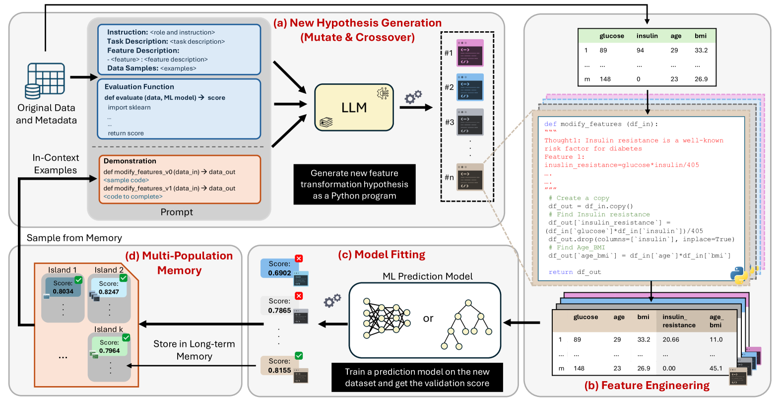
Figure 1: Overview of the LLM-FE Framework. For a given dataset, LLM-FE follows these steps: (a) New Hypothesis Generation, where an LLM generates feature transformation hypotheses as programs for a given tabular dataset; (b) Feature Engineering, where the feature transformation program is applied to the underlying dataset, resulting in a modified dataset; (c) Model Fitting, where a prediction model is fitted on the modified training set and evaluated on the corresponding validation set; (d) Multi-Population Memory, which maintains a buffer of high-scoring programs that act as in-context samples for LLM’s iterative refinement prompt.

To address these limitations, we propose LLM-FE, a novel framework integrating the capabilities of LLMs with tabular prediction models and evolutionary search to facilitate effective feature optimization. As shown in Figure 1, LLM-FE follows an iterative process to generate and evaluate the hypothesis of the feature transformation, using the performance of the tabular prediction model as a reward to enhance the generation of effective features. Starting from an initial feature transformation program, LLM-FE leverages the LLMs’ embedded domain knowledge by incorporating task-specific details, feature descriptions, and a subset of data samples to generate new feature discovery hypotheses (Figure 1(a)). At each iteration, LLM acts as a knowledge-guided evolutionary optimizer, which mutates examples of previously successful feature transformation programs to generate new effective features (Meyerson et al., 2024). The refined hypotheses are then evaluated by augmenting the original dataset with the proposed feature hypotheses (Figure 1(b)) and training a tabular prediction model on the augmented data (Figure 1(c)). The model’s performance, measured on a held-out validation set, provides data-driven feedback that, combined with a dynamic memory of previously explored feature transformation programs (Figure 1(d)), guides the LLM to refine its hypothesis generation iteratively.

Table 1 summarizes a list of distinguishing features of LLM-FE compared to the state-of-the-art classical and LLM-based feature engineering methods. Unlike prior methods that rely on either fixed rules or pure LLM generation, LLM-FE leverages LLMs’ domain knowledge to seed a flexible hypothesis space while employing evolutionary optimization to iteratively refine features. This facilitates open-ended feature discovery, generalizing effectively across both classification and regression tasks in tabular data prediction.

We evaluate LLM-FE with GPT-3.5-Turbo (OpenAI, 2023) and Llama-3.1-8B-Instruct (Dubey et al., 2024) backbones on classification and regression tasks across diverse tabular datasets. LLM-FE consistently outperforms the state-of-the-art feature engineering methods, identifying contextually relevant features that improve downstream performance. In particular, we observe improvements with tabular models like XGBoost (Chen & Guestrin, 2016), TabPFN (Hollmann et al., 2022), and MLP (Gorishniy et al., 2021). Our analysis also highlights the importance of evolutionary search in achieving effective results. The major contributions of this work can be summarized as follows.

$\bullet$ We introduce LLM-FE, a novel framework that leverages the LLM’s reasoning capabilities and domain knowledge, coupled with evolutionary search, to perform automated feature engineering for tabular data.

$\bullet$ Our experimental results demonstrate the effectiveness of LLM-FE, showcasing its ability to outperform state-of-the-art baselines across diverse benchmark datasets.

$\bullet$ Through a comprehensive ablation study, we highlight the critical role of domain knowledge, evolutionary search, data-driven feedback, and data samples in guiding the LLM to efficiently explore the feature space and discover impactful features more effectively.

Table 1: Comparison of the proposed LLM-FE with existing feature engineering methods.

Method	Classification	Regression	Domain	Evolutionary
			Knowledge	Refinement
AutoFeat	✓	✓	✗	✗
OpenFE	✓	✓	✗	✗
FeatLLM	✓	✗	✓	✗
CAAFE	✓	✗	✓	✗
LLM-FE	✓	✓	✓	✓

2 Related Works

Feature Engineering.

Feature engineering involves creating meaningful features from raw data to improve predictive performance (Hollmann et al., 2024). The growing complexity of datasets has driven the automation of feature engineering to reduce manual effort and optimize feature discovery. Traditional automated feature engineering methods include tree-based exploration (Khurana et al., 2016), iterative subsampling (Horn et al., 2020), and transformation enumeration (Kanter & Veeramachaneni, 2015). Learning-based methods leverage machine learning and reinforcement learning for feature transformation (Nargesian et al., 2017; Khurana et al., 2018; Zhang et al., 2019). OpenFE (Zhang et al., 2023) integrates a feature-boosting algorithm with a two-stage pruning strategy. These traditional approaches often fail to leverage domain knowledge for feature discovery, making LLMs well-suited for such tabular prediction tasks due to their prior contextual domain understanding.

LLMs and Optimization.

Recent advances in LLMs enable them to leverage their pre-trained knowledge to handle novel tasks through techniques such as prompt engineering and in-context learning without requiring additional training (Brown et al., 2020; Wei et al., 2022). Despite the progress made with LLMs, they often struggle with factually incorrect or inconsistent outputs (Madaan et al., 2024; Zhu et al., 2023). Researchers have thus explored methods that use feedback or refinement mechanisms to improve LLM responses and leverage them within complex optimization tasks (Madaan et al., 2024; Haluptzok et al., 2022). More recent approaches involving evolutionary optimization frameworks couple LLMs with evaluators (Lehman et al., 2023; Liu et al., 2024; Wu et al., 2024; Lange et al., 2024), using LLMs to perform adaptive mutation and crossover operations (Meyerson et al., 2024). This approach has shown success in areas such as prompt optimization (Yang et al., 2024; Guo et al., 2023), neural architecture search (Zheng et al., 2023; Chen et al., 2024), discovery of mathematical heuristics (Romera-Paredes et al., 2024), and symbolic regression (Shojaee et al., 2024). Building on these concepts, our LLM-FE framework utilizes an LLM as an evolutionary optimizer by coupling its prior knowledge with data-driven refinement to discover optimal features for the underlying tabular learning task.

LLMs for Tabular Learning.

The rich prior knowledge encapsulated in LLMs has been harnessed to analyze structured data by serializing tabular data into natural language formats (Dinh et al., 2022; Hegselmann et al., 2023; Wang et al., 2023). Existing approaches include table-specific tokenization methods to pre-train models for consistent performance across diverse datasets (Yan et al., 2024) or employ fine-tuning/few-shot examples via in-context learning (Dinh et al., 2022; Hegselmann et al., 2023; Nam et al., 2023) to adapt LLMs to tabular prediction tasks. Recent research has explored the potential of LLMs for feature engineering. FeatLLM (Han et al., 2024) improves tabular predictions by generating and parsing rules to engineer binary features. CAAFE (Hollmann et al., 2024) introduces a context-aware approach where LLMs generate features directly from task descriptions, while OCTree (Nam et al., 2024) incorporates an additional decision tree reasoning feedback to enhance feature engineering. We advance this line of research by leveraging LLMs to efficiently navigate the optimization space of feature discovery, generating meaningful features that are informed by prior knowledge and enriched with data-driven insights and evolutionary exploration.

3 LLM-FE

3.1 Problem Formulation

A tabular dataset $\mathcal{D}$ comprises $N$ rows (or instances), each characterized by $d$ columns (or features). Each data instance $x_{i}$ is a $d$-dimensional feature vector with feature names denoted by $C=\{c_{j}\}_{j=1}^{d}$. The dataset is accompanied by metadata $\mathcal{M}$, which contains feature descriptions and task-specific information. For supervised learning tasks, each instance $x_{i}$ is associated with a corresponding label $y_{i}$, where $y_{i}\in\{0,1,...,K\}$ for classification tasks with $K$ classes, and $y_{i}\in\mathbb{R}$ for regression tasks. Given a labeled tabular dataset $\mathcal{D}={(x_{i},y_{i})}_{i=1}^{N}$, the primary objective is to derive a prediction model $f$ through the empirical risk minimization process. This model $f$ is designed to establish a mapping from the input feature space $\mathcal{X}$ to its corresponding label space $\mathcal{Y}$:

$$\min_{f}\mathcal{L}_{f}(f(\mathcal{X}),\mathcal{Y})$$ (1)

where $\mathcal{L}_{f}$ is the loss function. Our objective in feature engineering is to determine an optimal feature transformation $\mathcal{T}$, which enhances the performance of a predictive model when trained on the transformed input space. Formally, the feature engineering task can be defined as:

$$\max_{\mathcal{T}}\mathcal{E}(f^{*}(\mathcal{T}(\mathcal{X}_{\text{val}})),\mathcal{Y}_{\text{val}})$$ (2)

subject to

$$f^{*}=\operatorname*{arg\,min}_{f}\mathcal{L}_{f}(f(\mathcal{T}(\mathcal{X}_{\text{train}})),\mathcal{Y}_{\text{train}})$$ (3)

where $\mathcal{T}$ is the feature transformation generated by the LLM $\pi_{\theta}$ and defined as $\mathcal{T}=\pi_{\theta}(\mathcal{X}_{train})$ meaning the transformation is learned from the training data by the LLM. The predictive model $f^{*}$ is then trained on the transformed training data $\mathcal{T}(\mathcal{X}_{train})$ to minimize loss. Consequently, the bilevel optimization problem seeks to identify the feature transformations $\mathcal{T}$ that maximize the performance $\mathcal{E}$ on the validation set $\mathcal{T}(\mathcal{X}_{\text{val}})$ while minimizing the loss function on the transformed training data, thereby efficiently exploring the potential feature space.

3.2 Hypothesis Generation

Figure 1(a) illustrates the hypothesis generation step that uses an LLM to create multiple new feature transformation programs, leveraging the model’s prior knowledge, reasoning, and in-context learning abilities to effectively explore the feature space.

3.2.1 Input Prompt

To facilitate the creation of effective and contextually relevant feature discovery programs, we develop a structured prompting methodology. The prompt is designed to provide comprehensive data-specific information, an initial feature transformation program for the evolution starting point, an evaluation function, and a well-defined output format (see Appendix B.2 for more details). Our input prompts $p$ are composed of the following key elements:

Instruction.

The LLM is assigned the task of finding the most relevant features to help solve the given regression/ classification problem. The task emphasizes using the LLM’s prior knowledge of the dataset’s domain to generate features. The LLM is explicitly instructed to generate novel features and provide clear step-by-step reasoning for their relevance to the prediction task.

Dataset Specification.

After providing the instructions, we provide LLM with the dataset-specific information from the metadata $\mathcal{M}$. This information encompasses a detailed description of the intended downstream task, along with the feature names $C$ and their corresponding descriptions. In addition, we provide a limited number of representative samples from the tabular dataset. To improve the effective interpretation of the data, we adopt the serialization approach used in previous works (Dinh et al., 2022; Hegselmann et al., 2023; Han et al., 2024). We serialized the data samples as follows:

$$\small\text{Serialize}(x_{i},y_{i},C)=$$

$$`\text{If }c_{1}\text{ is }x_{i}^{1},...,c_{d}\text{ is }x_{i}^{d}.~~\text{Then Result is }y_{i}\text{'}$$ (4)

By providing dataset-specific details, we guide the language model to focus on the most contextually pertinent features that directly support the dataset and task objective.

Evaluation Function.

The evaluation function, incorporated into the prompt, guides the language model to generate feature transformation programs that align with performance objectives. These programs augment the original dataset with new features, which are assessed on the basis of a prediction model’s performance when trained on the augmented data. The model’s evaluation score on the augmented validation set serves as an indicator of feature quality. By including the evaluation function in the prompt, the LLM generates programs that are inherently aligned with the desired performance criteria.

In-Context Demonstration.

Specifically, we sample the $k$ highest-performing demonstrations from previous iterations, enabling the LLM to build on successful outputs. The iterative interaction between the LLM’s generative outputs and the evaluator’s feedback, informed by these examples, facilitates a systematic refinement process. With each iteration, the LLM progressively improves its outputs by leveraging patterns and insights identified in previous successful demonstrations.

3.2.2 Hypothesis Sampling

At each iteration $t$, we construct the prompt $p_{t}$ by sampling the previous iteration as input to the LLM $\pi_{\theta}$, resulting in the output $\mathcal{T}_{1},\dots,\mathcal{T}_{b}=\pi_{\theta}(p_{t})$ representing a set of $b$ sampled programs. To promote diversity and maintain a balance between exploration (creativity) and exploitation (prior knowledge), we employ stochastic temperature-based sampling. Each of the sampled feature hypotheses ($\mathcal{T}_{i}$) is executed before evaluation to discard error-prone programs. This ensures that only valid and executable feature transformation programs are considered further in the optimization pipeline. In addition, to ensure computational efficiency, a maximum execution time threshold is enforced, discarding any programs that exceed it.

3.3 Data-Driven Evaluation

Following hypotheses generation, we use the generated hypotheses to augment the original dataset with the newly derived features (Figure 1(b)). As illustrated in Figure 1(c), the feature space evaluation process comprises two stages: (i) model training on the augmented dataset, and (ii) performance assessment using validation data. We fit a tabular predictive model $f^{*}$, to the transformed training set $\mathcal{T}(\mathcal{X}_{\text{tr}})$, by minimizing the loss $\mathcal{L}_{f}$ as shown in Eq.2. Subsequently, we evaluated the LLM-generated feature transformations $\mathcal{T}$ by evaluating the model’s performance on the augmented validation set $\mathcal{T}(\mathcal{X}_{\text{val}})$ (see Eqs. 2 and 3). As explained in Section 3.1, the objective is to find optimal features that maximize the performance $\mathcal{E}$, i.e. accuracy for classification tasks and error metrics for regression problems.

3.4 Memory Management

To promote diverse feature discovery and avoid stagnation in local optima, LLM-FE employs evolutionary multi-population memory management (Figure 1(d)) to store feature discovery programs in a dedicated database. Then, it uses samples from this database to construct in-context examples for LLM, facilitating the generation of novel hypotheses. This step consists of two components: (i) multi-population memory to maintain a long-term memory buffer, and (ii) sampling from this memory buffer to construct in-context example demonstrations. After evaluating the feature hypotheses in iteration $t$, we store the pair of hypotheses score ($\mathcal{T},s$) in the population buffer $\mathcal{P}_{t}$ to iteratively refine the search process. To effectively evolve a population of programs, we adopt a multi-population model inspired by the ‘island’ model employed by (Cranmer, 2023; Shojaee et al., 2024; Romera-Paredes et al., 2024). The program population is divided into $m$ independent islands, each evolving separately and initialized with a copy of the user’s initial example (see Figure 5(d)). This enables parallel exploration of the feature space, mitigating the risk of suboptimal solutions. At each iteration $t$, we select one of the $m$ islands and sample programs from the memory buffer to update the prompt with new in-context examples. The newly generated hypotheses samples $b$ are evaluated, and if their scores $s_{j}$ exceed the current best score, the hypotheses score pair ($\mathcal{T}_{j},s_{j}$) is added to the same island from which the in-context examples were sampled. To preserve diversity and ensure that programs with different performance characteristics are maintained in the buffer, we cluster programs within islands based on their signature, which is defined by their scores.

To build refinement prompts, we follow the sampling process from (Romera-Paredes et al., 2024), first sampling one of the $m$ available islands followed by sampling the $k$ programs from the selected island to create $k$-shot in-context examples for the LLM. Cluster selection prefers high-scoring programs and follows Boltzmann sampling (De La Maza & Tidor, 1992) with a score-based probability of choosing a cluster $i$: $P_{i}=\frac{exp(s_{i}/\tau_{c})}{\sum_{i}exp(s_{i}/\tau_{c})}$, where $s_{i}$ denotes the mean score of the $i$-th cluster and $\tau_{c}$ is the temperature parameter. The sampled feature transformation programs from the memory buffer are then included in the prompt as examples to guide LLM toward successful feature hypotheses. Refer to Appendix B.2 for more details.

Algorithm 1 presents the pseudocode of LLM-FE. We begin with the initialization of a memory buffer BufferInit, incorporating an initial population that contains a simple feature transform. This initialization serves as the starting point for the evolutionary search for feature transformation programs to be evolved in the subsequent steps. At each iteration $t$, the function topk is used to sample $k$ in-context examples from the population of the previous iteration $\mathcal{P}_{t-1}$ to update the prompt. Subsequently, we prompt the LLM using this updated prompt to sample $b$ new programs. The sampled programs are then evaluated using FeatureScore, which represents the Data-Driven Evaluation (Section 3.3). After $T$ iterations, the best-scoring program $\mathcal{T}^{*}$ from $\mathcal{P}_{t}$ and its corresponding score $s^{*}$ are returned as the optimal solution found for the problem. LLM-FE employs an iterative search to enhance programs, harnessing the LLM’s capabilities. Learning from the evolving pool of experiences in its buffer, the LLM steers the search toward effective solutions.

Algorithm 1 LLM-FE

0:  LLM $\pi_{\theta}$, Dataset $\mathcal{D}$, Metadata $\mathcal{M}$, Memory Buffer $\mathcal{P}$, Iterations $T$, Prediction model $f$, Performance Metric $\mathcal{E}$, Prompt template $p$

1:  # Initialize Memory Buffer

2:  $\mathcal{P}_{0}\leftarrow$ BufferInit()

3:  $\mathcal{T}^{*},s^{*}\leftarrow\text{null},\text{-}\infty$

4:  # Update Prompt template with Data and Metadata $p\leftarrow\texttt{UpdatePrompt}(\mathcal{D,M})$

5:  for $t=1,\dots,T-1$ do

6:  # Add $k$ examples from Memory Buffer to the Prompt

7:  $p_{t}=(p+\mathcal{P}_{t-1}.\texttt{topk}())$

8:  # Sample $b$ outputs from the LLM

9:  $\mathcal{T}_{1},\dots,\mathcal{T}_{b}\leftarrow\pi_{\theta}(p_{t})$

10:  # Evaluation and Buffer Update

11:  for $j=0,\dots,b$ do

12:   $s_{j}\leftarrow$ FeatureScore($f,\mathcal{T}_{j},\mathcal{D},\mathcal{E}$)

13:   if $s>s^{*}$ then

14:    $\mathcal{T}^{*},s^{*}\leftarrow\mathcal{T}_{j},s_{j}$

15:    $\mathcal{P}_{t}\leftarrow\texttt{UpdateBuffer}(\mathcal{P}_{t-1},\mathcal{T}_{j},s_{j})$

16:   end if

17:  end for

18:  end for

18:  $\mathcal{T}^{*},s^{*}$

4 Experimental Setup

Table 2: Performance of XGBoost on Classification Datasets using various Feature Engineering (FE) Methods, evaluated using accuracy (higher values indicate better performance). We report the mean values and standard deviation across five splits. ✗ : denotes failure for all runs due to execution errors. bold: indicates the best performance. underline: indicates the second-best performance. ‘n’: indicates the number of samples; ‘p’: indicates the number of features.

Dataset	n	p	Base	Classical FE Methods		LLM-based FE Methods		LLM-FE
				AutoFeat	OpenFE	CAAFE	FeatLLM
balance-scale	625	4	0.856 $\pm$ 0.020	0.925 $\pm$ 0.036	0.986 $\pm$ 0.009	0.966 $\pm$ 0.029	0.800 $\pm$ 0.037	0.990 $\pm$ 0.013
breast-w	699	9	0.956 $\pm$ 0.012	0.956 $\pm$ 0.019	0.956 $\pm$ 0.014	0.960 $\pm$ 0.009	0.967 $\pm$ 0.015	0.970 $\pm$ 0.009
blood-transfusion	748	4	0.742 $\pm$ 0.012	0.738 $\pm$ 0.014	0.747 $\pm$ 0.025	0.749 $\pm$ 0.017	0.771 $\pm$ 0.016	0.751 $\pm$ 0.036
car	1728	6	0.995 $\pm$ 0.003	0.998 $\pm$ 0.003	0.998 $\pm$ 0.003	0.999 $\pm$ 0.001	0.808 $\pm$ 0.037	0.999 $\pm$ 0.001
cmc	1473	9	0.528 $\pm$ 0.029	0.505 $\pm$ 0.015	0.517 $\pm$ 0.007	0.524 $\pm$ 0.016	0.479 $\pm$ 0.015	0.531 $\pm$ 0.015
credit-g	1000	20	0.751 $\pm$ 0.019	0.757 $\pm$ 0.017	0.758 $\pm$ 0.017	0.751 $\pm$ 0.020	0.707 $\pm$ 0.034	0.766 $\pm$ 0.015
eucalyptus	736	19	0.655 $\pm$ 0.024	0.664 $\pm$ 0.028	0.663 $\pm$ 0.033	0.679 $\pm$ 0.024	✗	0.668 $\pm$ 0.027
heart	918	11	0.858 $\pm$ 0.013	0.857 $\pm$ 0.021	0.854 $\pm$ 0.020	0.849 $\pm$ 0.023	0.865 $\pm$ 0.030	0.866 $\pm$ 0.021
pc1	1109	21	0.931 $\pm$ 0.004	0.931 $\pm$ 0.014	0.931 $\pm$ 0.009	0.929 $\pm$ 0.005	0.933 $\pm$ 0.007	0.935 $\pm$ 0.006
tic-tac-toe	958	9	0.998 $\pm$ 0.002	1.000 $\pm$ 0.000	0.994 $\pm$ 0.006	0.996 $\pm$ 0.003	0.653 $\pm$ 0.037	0.998 $\pm$ 0.005
vehicle	846	18	0.754 $\pm$ 0.016	0.788 $\pm$ 0.018	0.785 $\pm$ 0.008	0.771 $\pm$ 0.019	0.744 $\pm$ 0.035	0.761 $\pm$ 0.027
Mean Rank			–	3.18	3.09	3.00	3.82	1.54

Table 3: Performance of XGBoost on Regression Datasets using various Feature Engineering (FE) Methods, evaluated using normalized root mean square error (N-RMSE) (lower values indicate better performance). We report the mean values and standard deviation across five splits. ✗ : denotes failure for all runs due to execution errors. bold: indicates the best performance. underline: indicates the second-best performance. ‘n’: indicates the number of samples; ‘p’: indicates the number of features.

Dataset	n	p	Base	Classical FE Methods		LLM-FE
				AutoFeat	OpenFE
airfoil_self_noise	1503	6	0.013 $\pm$ 0.001	0.012 $\pm$ 0.001	0.013 $\pm$ 0.001	0.011 $\pm$ 0.001
bike	17389	11	0.216 $\pm$ 0.005	0.223 $\pm$ 0.006	0.216 $\pm$ 0.007	0.207 $\pm$ 0.006
cpu_small	8192	10	0.034 $\pm$ 0.003	0.034 $\pm$ 0.002	0.034 $\pm$ 0.002	0.033 $\pm$ 0.003
crab	3893	8	0.234 $\pm$ 0.009	0.228 $\pm$ 0.008	0.224 $\pm$ 0.001	0.223 $\pm$ 0.013
diamonds	53940	9	0.139 $\pm$ 0.002	0.140 $\pm$ 0.004	0.137 $\pm$ 0.002	0.134 $\pm$ 0.002
forest-fires	517	13	1.469 $\pm$ 0.080	1.468 $\pm$ 0.086	1.448 $\pm$ 0.113	1.417 $\pm$ 0.083
housing	20640	9	0.234 $\pm$ 0.009	0.231 $\pm$ 0.013	0.224 $\pm$ 0.005	0.218 $\pm$ 0.009
insurance	1338	7	0.397 $\pm$ 0.020	0.384 $\pm$ 0.024	0.383 $\pm$ 0.022	0.381 $\pm$ 0.028
plasma_retinol	315	13	0.390 $\pm$ 0.032	0.411 $\pm$ 0.036	0.392 $\pm$ 0.032	0.388 $\pm$ 0.033
wine	4898	10	0.110 $\pm$ 0.001	0.109 $\pm$ 0.001	0.108 $\pm$ 0.001	0.105 $\pm$ 0.001
Mean Rank			–	3.00	2.00	1.00

We evaluated LLM-FE on a range of tabular datasets, encompassing both classification and regression tasks. Our experimental analysis included quantitative comparisons with baselines and detailed ablation studies. Specifically, we assessed our approach using three known tabular predictive models with distinct architectures: (1) XGBoost, a tree-based model (Chen & Guestrin, 2016), (2) MLP, a neural model (Gorishniy et al., 2021), and (3) TabPFN (Hollmann et al., 2022), a transformer-based foundation model (Vaswani, 2017). The results highlight LLM-FE’s capability to generate effective features that consistently enhance the performance of different prediction models across diverse datasets.

4.1 Datasets

For our evaluation, we utilized two categories of datasets including (1) 11 classification datasets and (2) 10 regression datasets, each containing a mix of categorical and numerical features. Additionally, we included 8 large-scale, high-dimensional datasets to ensure a comprehensive evaluation of our method (see Appendix C.3). Following (Hollmann et al., 2024; Zhang et al., 2023), these datasets were sourced from well-known machine learning repositories, including OpenML (Vanschoren et al., 2014; Feurer et al., 2021), the UCI Machine Learning Repository (Asuncion et al., 2007), and Kaggle. Each dataset is accompanied by metadata, which includes a natural language description of the prediction task and descriptive feature names. We partitioned each dataset into training and testing sets using an 80-20 split. Following (Hollmann et al., 2024), we evaluated all methods over five iterations, each time using a distinct random seed and train-test splits. For more details, check Appendix 5.

4.2 Baselines

We evaluated LLM-FE against state-of-the-art feature engineering approaches, including OpenFE (Zhang et al., 2023) and AutoFeat (Horn et al., 2020), as well as LLM-based methods CAAFE (Hollmann et al., 2024) and FeatLLM (Han et al., 2024). We used XGBoost as the default tabular data prediction model in comparison between feature engineering baselines and employed GPT-3.5-Turbo as the default LLM backbone for all LLM-based methods. To ensure a fair comparison, all LLM-based baselines were configured to query the LLM backbone for a total of 20 samples until they converged to their best performance. Additional implementation details for all baselines are provided in Appendix B.1.

4.3 LLM-FE Configuration

In our experiments, we utilized GPT-3.5-Turbo and Llama-3.1-8B-Instruct as backbone LLMs, with a sampling temperature parameter of $t=0.8$ and the number of islands set to $m=3$. At each iteration, the LLM generated $b=3$ feature transformation programs per prompt in Python. To ensure consistency with baselines, LLM-FE was also configured with a total of 20 LLM samples for each experiment. Finally, we sampled the top $m$ (where $m$ denotes the number of islands) feature discovery programs based on their respective validation scores and reported the final prediction through an ensemble. More implementation details are provided in Appendix B.2.

5 Results and Discussion

5.1 Performance Comparisons

Evaluation on Classification Datasets.

In Table 2, we compare LLM-FE against various feature engineering baselines across 11 classification datasets. The results demonstrate that LLM-FE consistently enhances predictive performance from the base model (using raw data). LLM-FE also obtains the lowest mean rank, showing better effectiveness in enhancing feature discovery compared to other leading baselines. We have also extended our analysis to more complex datasets including high-dimensional and large-sample datasets to evaluate LLM-FE’s scalability in challenging scenarios. See Appendix C.3 for detailed results.

Evaluation on Regression Datasets.

To further evaluate the effectiveness of LLM-FE, we perform experiments on 10 regression datasets using the same evaluation settings employed for the classification datasets. The hypothesis space of current LLM-based baselines (CAAFE and FeatLLM) are only designed for classification datasets, so in this experiment, we only compare LLM-FE with non-LLM baselines (OpenFE and AutoFeat) which have been tested before for regression tasks. Table 3 compares the predictive performance using normalized root mean square error (N-RMSE). The results indicate that LLM-FE outperforms all baseline methods, achieving the lowest mean rank and consistently improving errors across all datasets.

5.2 Generalizability Analysis

To evaluate the generalizability of the LLM-FE framework, we examine its performance across multiple tabular prediction models and various LLM backbones. Specifically, we employ two LLM backbones, Llama-3.1-8B-Instruct and GPT-3.5-Turbo, in conjunction with three distinct tabular prediction models: XGBoost (Chen & Guestrin, 2016), a widely-used tree-based algorithm for tabular tasks; Multilayer Perceptron (MLP), a simple yet common deep-learning architecture tailored to tabular datasets (Gorishniy et al., 2021); and TabPFN (Hollmann et al., 2022), a recent transformer-based foundation model specifically designed for tabular data. Table 4 summarizes our findings, demonstrating that LLM-FE effectively identifies features that enhance the performance of various prediction models and LLM backbones across different tasks. Notably, the results indicate that features generated by LLM-FE using either LLM backbone consistently improve base model prediction performance compared to scenarios without any feature engineering. More detailed analyses of dataset-specific performances and feature transferability experiments are provided in Appendix C.1 and C.4.

Table 4: Performance improvement by LLM-FE using different prediction models and LLM backbones. We report the accuracy for classification tasks and normalized root mean square error for regression tasks. All results represent the mean and standard deviation computed across five splits. bold: indicates the best performance. TabPFN^∗ evaluations are conducted using only 10,000 samples due to its limited processing capacity.

Method	LLM	Classification $\uparrow$	Regression $\downarrow$
XGBoost
Base	–	0.820 $\pm$ 0.144	0.324 $\pm$ 0.016
LLM-FE	Llama 3.1-8B	0.832 $\pm$ 0.147	0.310 $\pm$ 0.022
	GPT-3.5 Turbo	0.840 $\pm$ 0.150	0.306 $\pm$ 0.015
MLP
Base	–	0.745 $\pm$ 0.193	0.871 $\pm$ 0.027
LLM-FE	Llama 3.1-8B	0.764 $\pm$ 0.173	0.794 $\pm$ 0.016
	GPT-3.5 Turbo	0.784 $\pm$ 0.175	0.631 $\pm$ 0.043
TabPFN∗
Base	–	0.852 $\pm$ 0.133	0.289 $\pm$ 0.016
LLM-FE	Llama 3.1-8B	0.856 $\pm$ 0.133	0.288 $\pm$ 0.016
	GPT-3.5 Turbo	0.863 $\pm$ 0.132	0.286 $\pm$ 0.015

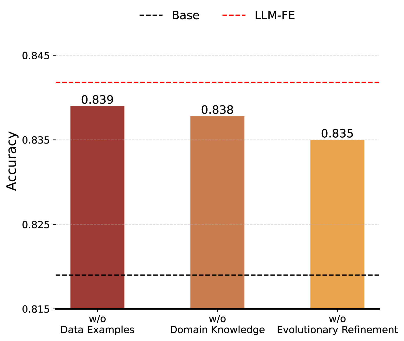
Figure 2: Aggregated ablation study results across classification datasets, showcasing the impact of individual components on LLM-FE’s performance: (a) Data Examples, (b) Domain Knowledge, and (c) Evolutionary Refinement. The model performance is measured using accuracy, with higher accuracy indicating better performance.

6 Analysis

6.1 Ablation Study

We perform an ablation study on the classification datasets listed in Table 2 to assess the contribution of each component in LLM-FE. Figure 2 illustrates the impact of individual components on overall performance, using XGBoost for prediction and GPT-3.5-Turbo as the LLM backbone. We report the accuracy aggregated over all the classification datasets. In the ‘w/o Domain Knowledge’ setting, dataset and task-specific details are removed from the prompt to assess the impact of domain knowledge on performance. Feature names are anonymized and replaced with generic placeholders such as C1, C2, $\dots$, Cn, effectively removing any semantic meaning that could provide contextual insights about the problem. Without domain knowledge, the classification performance significantly drops to 0.838, underscoring its critical role in generating meaningful features. Removing the evolutionary refinement (‘w/o Evolutionary Refinement’ setting) also leads to a considerable decline in performance, emphasizing the importance of iterative data-driven feedback in addition to domain knowledge for refining hypotheses. Lastly, ablation results show that eliminating data examples from the LLM prompt (‘w/o Data Examples’ variant) leads to only a slight performance drop across datasets. This suggests that providing data examples in the prompt offers limited benefit, as LLMs struggle to comprehend the nuances and patterns within the data samples. The best-performing variant (LLM-FE) demonstrates the positive contribution of each component including domain knowledge, evolutionary search, and example-based guidance in enhancing performance beyond the base model.

6.2 Qualitative Analysis

Impact of Evolutionary Refinement.

Figure 3 shows the detailed performance trajectory of LLM-FE compared with its ‘w/o Evolutionary Refinement’ variant on PC1 and Balance-Scale datasets. The graph demonstrates that LLM-FE, using evolutionary search, consistently improves validation accuracy, while the non-refinement variant stagnates due to local optima. On the PC1 dataset, the non-refinement variant plateaus after seven iterations, and on the Balance-Scale dataset, it stagnates after five iterations. LLM-FE’s evolutionary refinement helps it escape local optima with more robust optimization, leading to better validation accuracy on both datasets.

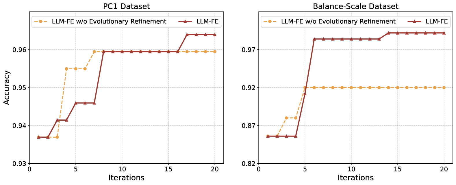
Figure 3: Performance Trajectory Analysis. Validation Accuracy progression for LLM-FE w/o evolutionary refinement and LLM-FE. LLM-FE demonstrates better validation accuracy, highlighting the advantage of evolutionary iterative refinement.

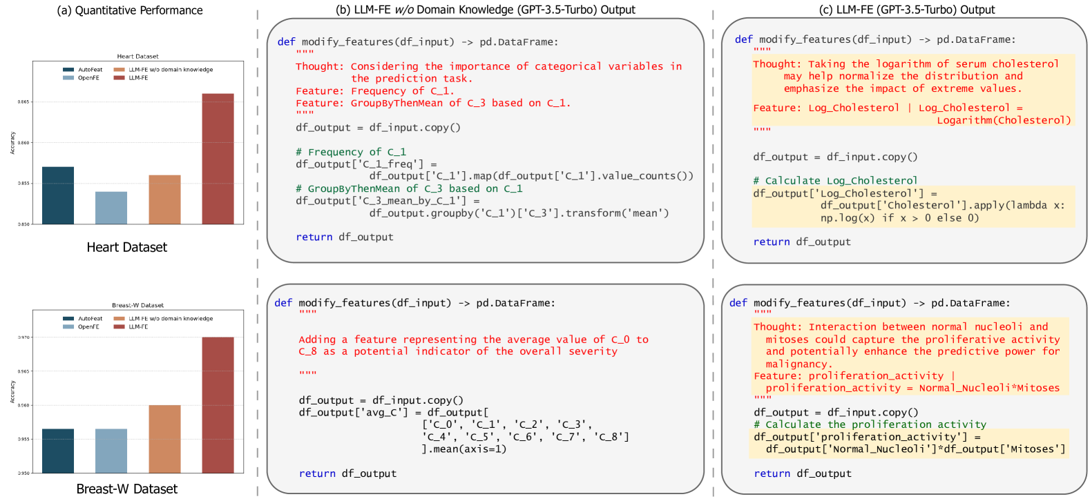
Figure 4: Quantitative and Qualitative Analysis on Impact of Domain Knowledge for LLM-FE on Heart and Breast-W datasets. (a) Comparison of XGBoost performance for LLM-FE against its domain-agnostic variant and traditional methods, such as OpenFE and AutoFeat, which do not integrate domain knowledge and exhibit reduced performance. (b) Features generated using the w/o Domain Knowledge variant of LLM-FE. (c) Feature discovery program generated by LLM-FE. The generated programs emphasize how incorporating domain expertise leads to more interpretable features that improve model performance.

Impact of Domain Knowledge.

Figure 4 highlights the qualitative and quantitative benefits of domain-specific feature transforms. We demonstrate this using two datasets: the Breast-W dataset, which focuses on distinguishing between benign and malignant tumors, and the Heart dataset, which predicts cardiovascular disease risk based on patient attributes. These tasks underscore the crucial role of domain knowledge in identifying meaningful features. Using embedded domain knowledge, LLM-FE not only significantly improves accuracy but also provides the reasoning for choosing the given feature, leading to more interpretable feature engineering. For example, in the Heart dataset, LLM-FE suggests the feature ‘Log_Cholesterol’, recognizing cholesterol’s critical role in heart health and applying a logarithmic transformation to reduce the impact of outliers and stabilize the variance. In contrast, the ‘w/o Domain Knowledge’ variant arbitrarily combines existing features, leading to uninterpretable transformations and reduced overall performance (Figure 4 (a)). Similarly, for breast cancer prediction, LLM-FE identifies ‘proliferation_activity’ a biologically relevant metric leading to performance improvement, whereas the absence of domain knowledge results in a simple mean of all features, lacking interpretability and clinical significance (Figures 4(b) and 4(c)).

7 Conclusion

In this work, we introduce a novel framework LLM-FE that leverages LLMs as evolutionary optimizers to discover new features for tabular prediction tasks. By combining LLM-driven hypothesis generation with data-driven feedback and evolutionary search, LLM-FE effectively automates the feature engineering process. Through comprehensive experiments on diverse tabular learning tasks, we demonstrate that LLM-FE consistently outperforms state-of-the-art baselines, delivering substantial improvements in predictive performance across various tabular prediction models. Future work could explore integrating more powerful or domain-specific language models to enhance the relevance and quality of generated features for domain-specific problems. Moreover, our framework could extend beyond feature engineering to other stages of the tabular learning and data-centric pipeline, such as data augmentation, automated data cleaning (including imputation and outlier detection), and model tuning.

Impact Statement

The introduction of LLM-FE as a framework for leveraging LLMs in automated feature engineering has the potential to significantly impact the field of machine learning for tabular data by improving predictive performance and reducing the manual effort involved in feature engineering. This is particularly beneficial in resource-intensive domains where efficient feature extraction and transformation are crucial for accelerating model development. By combining domain expertise with evolutionary optimization, LLM-FE improves over existing methods, which often struggle to identify optimal feature transformations. While LLM-FE currently targets feature engineering, its potential could be extended to broader data-centric AI tasks. Future extensions could include automated data cleaning (such as imputation and outlier detection), exploratory data analysis, and data augmentation, further strengthening the quality and robustness of datasets in tabular learning. LLM-FE could also be extended to support model tuning and hyperparameter optimization, contributing to a more streamlined and interpretable machine learning pipeline and improving the generalization of the model.

Reproducibility Statement

To ensure the reproducibility of our work, we provide comprehensive implementation details of LLM-FE. Section 3 outlines the full methodology, while Appendix B.2 offers an in-depth description of the framework, including the specific LLM prompts used. The datasets employed in our experiments are also detailed in Appendix 5. Additionally, we plan to release our code and data at this repository to facilitate further research.

Appendix A Dataset Details

Table 5 describes the diverse collection of datasets spanning three major categories: (1) binary classification, (2) multi-class classification, and (3) regression problems used in our evaluation. The datasets were primarily sourced from established platforms, including OpenML (Vanschoren et al., 2014; Feurer et al., 2021), UCI (Asuncion et al., 2007), and Kaggle. We specifically selected datasets with descriptive feature names, excluding those with merely numerical identifiers. Each dataset includes a task description, enhancing contextual understanding for users. Our selection encompasses not only small datasets but also larger ones, featuring extensive data samples and high-dimensional datasets with over 50 features. This diverse and comprehensive selection of datasets represents a broad spectrum of real-world scenarios, varying in both feature dimensionality and sample size, thereby providing a robust framework for evaluating feature engineering works.

Table 5: Dataset statistics.

Dataset	#Features	#Samples	Source	ID/Name
Binary Classification
adult	14	48842	OpenML	1590
blood-transfusion	4	748	OpenML	1464
bank-marketing	16	45211	OpenML	1461
breast-w	9	699	OpenML	15
credit-g	20	1000	OpenML	31
tic-tac-toe	9	958	OpenML	50
pc1	21	1109	OpenML	1068
Multi-class Classification
arrhythmia	279	452	OpenML	5
balance-scale	4	625	OpenML	11
car	6	1728	OpenML	40975
cmc	9	1473	OpenML	23
eucalyptus	19	736	OpenML	188
jungle_chess	6	44819	OpenML	41027
vehicle	18	846	OpenML	54
cdc diabetes	21	253680	Kaggle	diabetes-health-indicators-dataset
heart	11	918	Kaggle	heart-failure-prediction
communities	103	1994	UCI	communities-and-crime
myocardial	111	1700	UCI	myocardial-infarction-complications
Regression
airfoil_self_noise	6	1503	OpenML	44957
cpu_small	12	8192	OpenML	562
diamonds	9	53940	OpenML	42225
plasma_retinol	13	315	OpenML	511
forest-fires	13	517	OpenML	42363
housing	9	20640	OpenML	43996
crab	8	3893	Kaggle	crab-age-prediction
insurance	7	1338	Kaggle	us-health-insurancedataset
bike	11	17389	UCI	bike-sharing-dataset
wine	10	4898	UCI	wine-quality

Appendix B Implementation Details

B.1 Baselines

We implement and evaluate various state-of-the-art feature engineering baselines, spanning traditional methods to recent LLM-based approaches, for comparison with LLM-FE. After generating features with each baseline, we apply a unified preprocessing pipeline to prepare the data for training and evaluation in the machine learning model. We implement the following baselines:

AutoFeat.

AutoFeat is a classical feature engineering approach that uses iterative feature subsampling with beam search to select informative features. We utilize the open-source autofeat package, retaining the default parameter settings. For parameter settings, we refer to the example ‘.ipynb’ files provided in their official repository.

OpenFE.

OpenFE is another state-of-the-art traditional feature engineering method using feature boosting and pruning algorithms. We employ the open-source openfe package with standard parameter settings.

FeatLLM.

FeatLLM uses an LLM to generate rules to binarize features that are then used as input to a simple model such as linear regression. We adapt the open-source featllm implementation, modifying the pipeline to use an XGBoost model for inference. To ensure a fair comparison with other methods, we provide the entire training dataset to train the XGBoost model while using only a subset of the dataset (10 samples) to the LLM to generate binary features. We report the results through an ensemble over three samples to maintain consistency with LLM-FE.

CAAFE.

We utilize the official implementation of CAAFE, maintaining all parameter settings as specified in the original repository. Following their workflow, we preprocess the data using their pipeline before inputting them into the prediction model after the feature engineering process.

B.2 LLM-FE

Hypothesis Generation.

Figure 5 presents an example prompt for the balance-scale dataset. The prompt begins with general instructions, followed by dataset-specific details, such as task descriptions, feature descriptions, and a subset of data instances serialized and expressed in natural language. To introduce diversity in prompting, we randomly sample between this approach and an alternative set of instructions, encouraging the LLM to explore a wider range of operators from OpenFE (Zhang et al., 2023), as prior LLMs tend to favor simpler operators (Küken et al., 2024) (see Figure 6). By providing this structured context, the model can leverage its domain knowledge to generate semantically and contextually meaningful hypotheses for new feature optimization programs.

Data-Driven Evaluation.

After prompting the LLM, we sample $b=3$ outputs. Based on preliminary experiments, we set the temperature for LLM output generation to $t=0.8$ to balance creativity (exploration) and adherence to problem constraints, as well as reliance on prior knowledge (exploitation). The data modification process is illustrated in Figure 5(c), where the outputs are used to modify the features via modify_features(input). These modified features are then input into a prediction model, and the resulting validation score is calculated. To ensure efficiency, our evaluation is constrained by time and memory limits set at $T=30$ seconds and $M=2GB$, respectively. Programs exceeding these limits are disqualified and assigned None scores, ensuring timely progress and resource efficiency in the search process.

Memory Management.

Following the ‘islands’ model used by (Cranmer, 2023; Shojaee et al., 2024; Romera-Paredes et al., 2024), we maintain the generated hypotheses along with their evaluation scores in a memory buffer comprising multiple islands ($m=3$) that evolve independently. Each island is initialized with a basic feature transformation program specific to the dataset. Each island is initialized with a simple feature transformation program specific to the dataset (def modify_features_v0()in Figure 5(d)). In each iteration, novel hypotheses and their validation metrics are incorporated into their respective islands only if they exceed the island’s current best score. Within each island, we additionally cluster feature discovery programs based on their signature, characterized by their validation score. Feature transformation programs that produce identical scores are consolidated together, creating distinct clusters. This clustering approach helps preserve diversity by ensuring that programs with varying performance characteristics remain in the population. We leverage this island model to construct prompts for the LLM. After an initial update of the prompt template with dataset-specific information, we integrate in-context demonstrations from the buffer. Following (Shojaee et al., 2024; Romera-Paredes et al., 2024), we randomly select one of the $m$ available islands. Within the chosen island, we sample $k=2$ programs to serve as in-context examples. To sample programs, we first select clusters based on their signatures using the Boltzmann selection strategy (De La Maza & Tidor, 1992) to sample clusters based on their signatures with a preference for clusters with higher scores. Let $s_{i}$ be the score of the i-th cluster, and probability $P_{i}$ for selecting i-th cluster is given as:

$$P_{i}=\frac{exp(\frac{s_{i}}{\tau_{c}})}{\sum_{i}(\frac{s_{i}}{\tau_{c}})},\text{ where }\tau_{c}=T_{0}(1-\frac{u\text{ mod }N}{N})$$ (5)

where $\tau_{c}$ is the temperature parameter, $u$ is the current number of programs on the island, and $T_{0}=0.1$ and $N=10,000$ are hyperparameters. Once a cluster is selected, we sample the programs from it.

Figure 5: Example of an input prompt for balance-scale dataset containing (a) instruction, (b) dataset specification containing the details about the task, features, and data samples, (c) evaluation function, (d) initial in-context demonstration, and (e) function to complete.

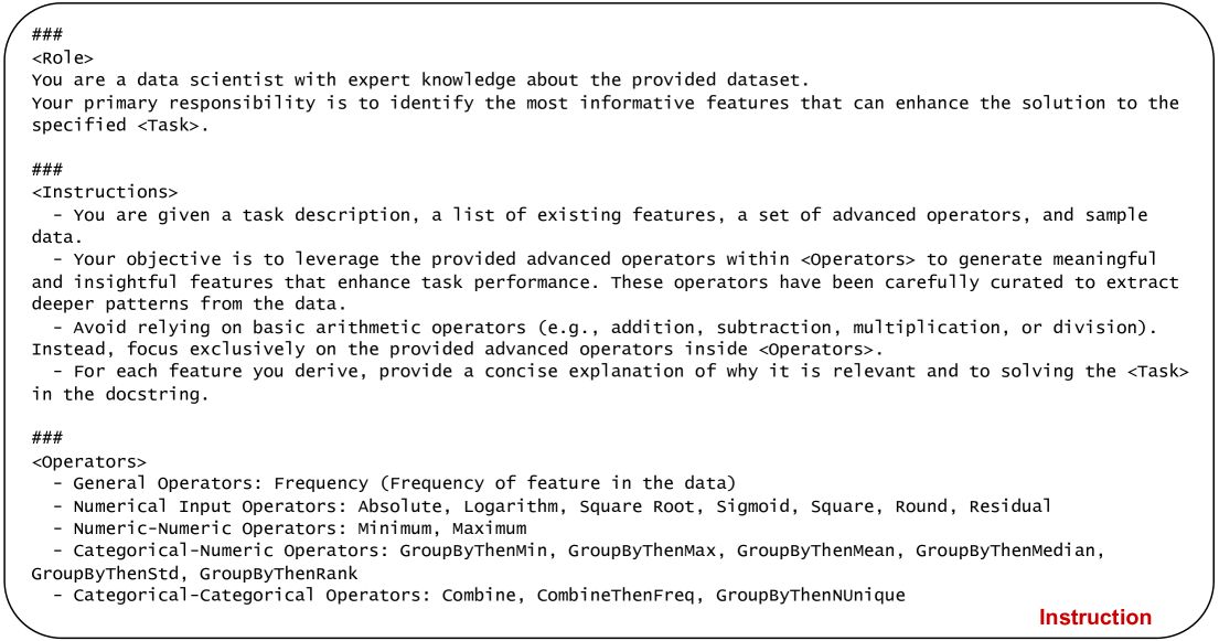
Figure 6: An example of the alternate set of instructions used to direct the model to use a complex set of operations over simple operators for generating features.

Appendix C Additional Analysis

C.1 Transferability of Generated Features

While traditional approaches typically use the same model for both feature generation and inference, we demonstrate that the features generated by one model can be utilized by other models. Following (Nam et al., 2024), we use XGBoost, a computationally efficient decision tree-based model, to generate features to be used by more complex architectures for inference. As demonstrated in Table 6, XGBoost-generated features show an improvement in the performance of MLP and TabPFN over its base versions. This cross-architecture performance improvement suggests that the generated features capture meaningful data characteristics that are valuable across different modeling paradigms.

Table 6: Comparative analysis of LLM-FE using feature transfer. We use XGBoost to perform feature engineering and apply these features to MLP and TabPFN inference models (indicated as LLM-FE _XGB). We report the accuracy for classification tasks and normalized root mean square error for regression tasks. We report the mean values and standard deviation across five random splits. bold: indicates the best performance.

Method	LLM	Classification $\uparrow$	Regression $\downarrow$
MLP
Base	–	0.745 $\pm$ 0.193	0.871 $\pm$ 0.027
LLM-FEXGB	GPT-3.5-Turbo	0.763 $\pm$ 0.216	0.848 $\pm$ 0.017
LLM-FE	GPT-3.5-Turbo	0.784 $\pm$ 0.175	0.631 $\pm$ 0.043
TabPFN
Base	–	0.852 $\pm$ 0.133	0.289 $\pm$ 0.016
LLM-FEXGB	GPT-3.5-Turbo	0.861 $\pm$ 0.136	0.287 $\pm$ 0.015
LLM-FE	GPT-3.5-Turbo	0.863 $\pm$ 0.132	0.286 $\pm$ 0.015

C.2 Robustness to Noise

Noise is an inherent challenge in real-world data, arising from various sources, including sensor errors, human mistakes, environmental factors, and equipment limitations. Such noise can mask underlying patterns and impair machine learning models’ ability to learn true relationships in the data. To evaluate how effectively LLM-FE leverages prior knowledge and evolutionary search to handle noisy data, we introduced Gaussian noise ($\sigma$ = 0, 0.01, 0.05, 0.1) into numerical classification datasets. As shown in Figure 7, we compared XGBoost’s performance across different feature engineering approaches, using GPT-3.5-Turbo as the LLM backbone for both the LLM-based approaches. The results demonstrate that LLM-FE maintains superior accuracy and robustness even under increasing noise conditions.

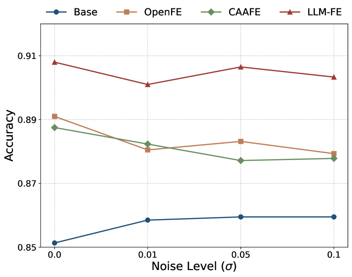
Figure 7: Impact of Noise Levels on XGBoost model performance across different feature engineering approaches, under increasing noise conditions ($\sigma=0.0\text{ to }0.1$). We report the mean accuracy across six classification datasets containing only numerical features.

C.3 Scalability Analysis

In addition to smaller classification datasets (see Section 5), we evaluate the effectiveness of our method on more complex datasets, including (1) high-dimensional datasets with a large number of features and (2) large-scale datasets with a substantial number of instances. We report the performance of the XGBoost model on these classification datasets using accuracy. For LLM-based methods, we utilize GPT-3.5-Turbo as the LLM backbone. Based on the findings from Section 5, we select the best-performing traditional feature engineering approach (OpenFE) and LLM-based baseline (CAAFE) for comparison with LLM-FE.

Table 7: Performance of XGBoost on complex datasets using various Feature Engineering Methods on (1) High-dimensional classification datasets, and (2) Large-scale classification datasets, evaluated using accuracy (higher values indicate better performance). We report the mean values and standard deviation across five random splits. ✗ : denotes failure for all runs due to execution errors. bold: indicates the best performance. underline: indicates the second-best performance. ‘n’: indicates the number of samples; ‘p’: indicates the number of features.

	n	p	Base	OpenFE	CAAFE	LLM-FE
Large scale datasets
adult	48.8k	14	0.873 $\pm$ 0.002	0.873 $\pm$ 0.002	0.872 $\pm$ 0.002	0.874 $\pm$ 0.003
bank-marketing	45.2k	16	0.906 $\pm$ 0.003	0.908 $\pm$ 0.002	0.907 $\pm$ 0.002	0.907 $\pm$ 0.002
cdc diabetes	253k	21	0.849 $\pm$ 0.001	0.849 $\pm$ 0.001	0.849 $\pm$ 0.001	0.849 $\pm$ 0.001
jungle_chess	44.8k	6	0.869 $\pm$ 0.001	0.900 $\pm$ 0.004	0.901 $\pm$ 0.038	0.969 $\pm$ 0.004
High dimensional datasets
covtype	581k	54	0.870 $\pm$ 0.001	0.885 $\pm$ 0.007	0.872 $\pm$ 0.003	0.882 $\pm$ 0.003
communities	1.9k	103	0.706 $\pm$ 0.016	0.704 $\pm$ 0.009	0.707 $\pm$ 0.013	0.711 $\pm$ 0.012
arrhythmia	452	279	0.657 $\pm$ 0.019	✗	✗	0.659 $\pm$ 0.018
myocardial	1.7k	111	0.784 $\pm$ 0.023	0.787 $\pm$ 0.026	0.789 $\pm$ 0.023	0.789 $\pm$ 0.023
Mean Rank			–	2.13	2.00	1.25

Analysis over high-dimensional dataset.

High-dimensional data in machine learning presents unique challenges due to the ‘curse of dimensionality’, where an increase in the feature space leads to sparse data distributions. This sparsity can degrade model performance and complicate feature engineering, making it difficult to identify relevant features and generate new ones to support the downstream task. To evaluate high-dimensional datasets, we focus on datasets containing more than 50 features as part of our analysis. As shown in Table 7, the general trend is that model performance gradually degrades as the number of features increases, though there are exceptions. Our LLM-FE framework addresses these challenges by carefully balancing dimensionality reduction with the retention of meaningful information, ensuring robust model generalization. Notably, our framework outperforms all feature engineering baselines for XGBoost.

Analysis over large-scale dataset.

Large-scale datasets present unique challenges compared to high-dimensional data. While a large number of samples can help reduce overfitting, the sheer volume of data can diminish the ability to identify and extract meaningful insights. Furthermore, even when meaningful features are identifiable, their impact may be reduced due to the dataset’s size. Features that perform well on smaller subsets may struggle to generalize across the entire distribution. Table 7 illustrates these challenges, showing how the presence of a large number of samples can obscure underlying patterns, making improvements from feature engineering negligible. Despite these challenges, LLM-FE shows better results compared to other baseline methods.

C.4 More Details About the Results

We extend the results from Section 5, showcasing the performance improvements achieved by LLM-FE across various prediction models. Specifically, we employ XGBoost, MLP, and TabPFN to generate features and subsequently use the same models for inference. As shown in Table 8, the features using GPT-3.5-Turbo by LLM-FE consistently enhance model performance across different datasets, outperforming the base versions trained without feature engineering.

Table 8: Performance improvement with LLM-FE. We report the mean and standard deviation over five splits. We use Normalized Root Mean Square Error for all regression datasets, with a lower value indicating better performance, and Accuracy for classification datasets, with a higher value indicating better performance. bold: indicates the best performance.

Dataset	XGBoost		MLP		TabPFN
	Base	LLM-FE	Base	LLM-FE	Base	LLM-FE
Classification Datasets
balance-scale	0.856 $\pm$ 0.020	0.990 $\pm$ 0.013	0.933 $\pm$ 0.008	0.997 $\pm$ 0.004	0.970 $\pm$ 0.016	1.000 $\pm$ 0.000
breast-w	0.956 $\pm$ 0.012	0.970 $\pm$ 0.009	0.957 $\pm$ 0.010	0.964 $\pm$ 0.005	0.971 $\pm$ 0.006	0.971 $\pm$ 0.007
blood-transfusion	0.742 $\pm$ 0.012	0.751 $\pm$ 0.036	0.674 $\pm$ 0.071	0.782 $\pm$ 0.017	0.790 $\pm$ 0.012	0.791 $\pm$ 0.011
car	0.995 $\pm$ 0.003	0.999 $\pm$ 0.001	0.929 $\pm$ 0.019	0.950 $\pm$ 0.009	0.984 $\pm$ 0.007	0.996 $\pm$ 0.006
cmc	0.528 $\pm$ 0.030	0.531 $\pm$ 0.015	0.559 $\pm$ 0.028	0.566 $\pm$ 0.028	0.563 $\pm$ 0.030	0.566 $\pm$ 0.036
credit-g	0.751 $\pm$ 0.019	0.766 $\pm$ 0.025	0.558 $\pm$ 0.144	0.633 $\pm$ 0.101	0.728 $\pm$ 0.008	0.794 $\pm$ 0.022
eucalyptus	0.655 $\pm$ 0.024	0.668 $\pm$ 0.027	0.414 $\pm$ 0.064	0.456 $\pm$ 0.062	0.712 $\pm$ 0.016	0.715 $\pm$ 0.021
heart	0.858 $\pm$ 0.013	0.866 $\pm$ 0.021	0.840 $\pm$ 0.010	0.844 $\pm$ 0.006	0.882 $\pm$ 0.025	0.880 $\pm$ 0.021
pc1	0.931 $\pm$ 0.004	0.935 $\pm$ 0.006	0.931 $\pm$ 0.002	0.904 $\pm$ 0.055	0.936 $\pm$ 0.007	0.937 $\pm$ 0.003
tic-tac-toe	0.998 $\pm$ 0.004	0.998 $\pm$ 0.005	0.816 $\pm$ 0.029	0.854 $\pm$ 0.052	0.984 $\pm$ 0.005	0.986 $\pm$ 0.009
vehicle	0.754 $\pm$ 0.016	0.761 $\pm$ 0.027	0.583 $\pm$ 0.062	0.673 $\pm$ 0.043	0.852 $\pm$ 0.016	0.856 $\pm$ 0.028
Regression Datasets
airfoil_self_noise	0.013 $\pm$ 0.001	0.011 $\pm$ 0.001	0.275 $\pm$ 0.008	0.108 $\pm$ 0.001	0.008 $\pm$ 0.001	0.007 $\pm$ 0.001
bike	0.216 $\pm$ 0.005	0.207 $\pm$ 0.005	0.636 $\pm$ 0.015	0.551 $\pm$ 0.022	0.200 $\pm$ 0.005	0.199 $\pm$ 0.006
cpu_small	0.034 $\pm$ 0.003	0.033 $\pm$ 0.003	3.793 $\pm$ 0.731	2.360 $\pm$ 1.263	0.036 $\pm$ 0.001	0.035 $\pm$ 0.001
crab	0.234 $\pm$ 0.009	0.223 $\pm$ 0.014	0.214 $\pm$ 0.010	0.212 $\pm$ 0.011	0.208 $\pm$ 0.013	0.207 $\pm$ 0.014
diamond	0.139 $\pm$ 0.002	0.134 $\pm$ 0.002	0.296 $\pm$ 0.018	0.265 $\pm$ 0.011	0.132 $\pm$ 0.005	0.130 $\pm$ 0.005
forest-fires	1.469 $\pm$ 0.080	1.417 $\pm$ 0.083	1.423 $\pm$ 0.104	1.344 $\pm$ 0.091	1.270 $\pm$ 0.101	1.269 $\pm$ 0.114
housing	0.234 $\pm$ 0.009	0.218 $\pm$ 0.009	0.505 $\pm$ 0.009	0.444 $\pm$ 0.036	0.210 $\pm$ 0.004	0.202 $\pm$ 0.003
insurance	0.397 $\pm$ 0.144	0.381 $\pm$ 0.142	0.896 $\pm$ 0.053	0.487 $\pm$ 0.026	0.351 $\pm$ 0.018	0.346 $\pm$ 0.020
plasma_retinol	0.390 $\pm$ 0.032	0.388 $\pm$ 0.033	0.440 $\pm$ 0.070	0.411 $\pm$ 0.053	0.348 $\pm$ 0.048	0.348 $\pm$ 0.055
wine	0.110 $\pm$ 0.001	0.105 $\pm$ 0.001	0.125 $\pm$ 0.001	0.125 $\pm$ 0.013	0.117 $\pm$ 0.004	0.116 $\pm$ 0.004

References

- Anaconda (2020) Anaconda. The state of data science 2020. Website, 2020. URL https://www.anaconda.com/state-of-data-science-2020.
- Asuncion et al. (2007) Asuncion, A., Newman, D., et al. Uci machine learning repository, 2007.
- Brown et al. (2020) Brown, T., Mann, B., Ryder, N., Subbiah, M., Kaplan, J. D., Dhariwal, P., Neelakantan, A., Shyam, P., Sastry, G., Askell, A., et al. Language models are few-shot learners. Advances in neural information processing systems, 33:1877–1901, 2020.
- Chen et al. (2024) Chen, A., Dohan, D., and So, D. Evoprompting: language models for code-level neural architecture search. Advances in Neural Information Processing Systems, 36, 2024.
- Chen & Guestrin (2016) Chen, T. and Guestrin, C. Xgboost: A scalable tree boosting system. In Proceedings of the 22nd acm sigkdd international conference on knowledge discovery and data mining, pp. 785–794, 2016.
- Cranmer (2023) Cranmer, M. Interpretable machine learning for science with pysr and symbolicregression. jl. arXiv preprint arXiv:2305.01582, 2023.
- De La Maza & Tidor (1992) De La Maza, M. and Tidor, B. Increased flexibility in genetic algorithms: The use of variable boltzmann selective pressure to control propagation. In Computer Science and Operations Research, pp. 425–440. Elsevier, 1992.
- Dinh et al. (2022) Dinh, T., Zeng, Y., Zhang, R., Lin, Z., Gira, M., Rajput, S., Sohn, J.-y., Papailiopoulos, D., and Lee, K. Lift: Language-interfaced fine-tuning for non-language machine learning tasks. Advances in Neural Information Processing Systems, 35:11763–11784, 2022.
- Domingos (2012) Domingos, P. A few useful things to know about machine learning. Communications of the ACM, 55(10):78–87, 2012.
- Dubey et al. (2024) Dubey, A., Jauhri, A., Pandey, A., Kadian, A., Al-Dahle, A., Letman, A., Mathur, A., Schelten, A., Yang, A., Fan, A., et al. The llama 3 herd of models. arXiv preprint arXiv:2407.21783, 2024.
- Feurer et al. (2021) Feurer, M., Van Rijn, J. N., Kadra, A., Gijsbers, P., Mallik, N., Ravi, S., Müller, A., Vanschoren, J., and Hutter, F. Openml-python: an extensible python api for openml. Journal of Machine Learning Research, 22(100):1–5, 2021.
- Gorishniy et al. (2021) Gorishniy, Y., Rubachev, I., Khrulkov, V., and Babenko, A. Revisiting deep learning models for tabular data. Advances in Neural Information Processing Systems, 34:18932–18943, 2021.
- Grinsztajn et al. (2022) Grinsztajn, L., Oyallon, E., and Varoquaux, G. Why do tree-based models still outperform deep learning on typical tabular data? Advances in neural information processing systems, 35:507–520, 2022.
- Guo et al. (2023) Guo, Q., Wang, R., Guo, J., Li, B., Song, K., Tan, X., Liu, G., Bian, J., and Yang, Y. Connecting large language models with evolutionary algorithms yields powerful prompt optimizers. arXiv preprint arXiv:2309.08532, 2023.
- Haluptzok et al. (2022) Haluptzok, P., Bowers, M., and Kalai, A. T. Language models can teach themselves to program better. arXiv preprint arXiv:2207.14502, 2022.
- Han et al. (2024) Han, S., Yoon, J., Arik, S. O., and Pfister, T. Large language models can automatically engineer features for few-shot tabular learning. arXiv preprint arXiv:2404.09491, 2024.
- Hegselmann et al. (2023) Hegselmann, S., Buendia, A., Lang, H., Agrawal, M., Jiang, X., and Sontag, D. Tabllm: Few-shot classification of tabular data with large language models. In International Conference on Artificial Intelligence and Statistics, pp. 5549–5581. PMLR, 2023.
- Hollmann et al. (2022) Hollmann, N., Müller, S., Eggensperger, K., and Hutter, F. Tabpfn: A transformer that solves small tabular classification problems in a second. arXiv preprint arXiv:2207.01848, 2022.
- Hollmann et al. (2024) Hollmann, N., Müller, S., and Hutter, F. Large language models for automated data science: Introducing caafe for context-aware automated feature engineering. Advances in Neural Information Processing Systems, 36, 2024.
- Horn et al. (2020) Horn, F., Pack, R., and Rieger, M. The autofeat python library for automated feature engineering and selection. In Machine Learning and Knowledge Discovery in Databases: International Workshops of ECML PKDD 2019, Würzburg, Germany, September 16–20, 2019, Proceedings, Part I, pp. 111–120. Springer, 2020.
- Kanter & Veeramachaneni (2015) Kanter, J. M. and Veeramachaneni, K. Deep feature synthesis: Towards automating data science endeavors. In 2015 IEEE international conference on data science and advanced analytics (DSAA), pp. 1–10. IEEE, 2015.
- Khurana et al. (2016) Khurana, U., Turaga, D., Samulowitz, H., and Parthasrathy, S. Cognito: Automated feature engineering for supervised learning. In 2016 IEEE 16th international conference on data mining workshops (ICDMW), pp. 1304–1307. IEEE, 2016.
- Khurana et al. (2018) Khurana, U., Samulowitz, H., and Turaga, D. Feature engineering for predictive modeling using reinforcement learning. In Proceedings of the AAAI Conference on Artificial Intelligence, volume 32, 2018.
- Küken et al. (2024) Küken, J., Purucker, L., and Hutter, F. Large language models engineer too many simple features for tabular data. arXiv preprint arXiv:2410.17787, 2024.
- Lange et al. (2024) Lange, R., Tian, Y., and Tang, Y. Large language models as evolution strategies. In Proceedings of the Genetic and Evolutionary Computation Conference Companion, pp. 579–582, 2024.
- Lehman et al. (2023) Lehman, J., Gordon, J., Jain, S., Ndousse, K., Yeh, C., and Stanley, K. O. Evolution through large models. In Handbook of Evolutionary Machine Learning, pp. 331–366. Springer, 2023.
- Liu et al. (2024) Liu, T., Astorga, N., Seedat, N., and van der Schaar, M. Large language models to enhance bayesian optimization. arXiv preprint arXiv:2402.03921, 2024.
- Madaan et al. (2024) Madaan, A., Tandon, N., Gupta, P., Hallinan, S., Gao, L., Wiegreffe, S., Alon, U., Dziri, N., Prabhumoye, S., Yang, Y., et al. Self-refine: Iterative refinement with self-feedback. Advances in Neural Information Processing Systems, 36, 2024.
- Meyerson et al. (2024) Meyerson, E., Nelson, M. J., Bradley, H., Gaier, A., Moradi, A., Hoover, A. K., and Lehman, J. Language model crossover: Variation through few-shot prompting. ACM Transactions on Evolutionary Learning, 4(4):1–40, 2024.
- Nam et al. (2023) Nam, J., Tack, J., Lee, K., Lee, H., and Shin, J. Stunt: Few-shot tabular learning with self-generated tasks from unlabeled tables. arXiv preprint arXiv:2303.00918, 2023.
- Nam et al. (2024) Nam, J., Kim, K., Oh, S., Tack, J., Kim, J., and Shin, J. Optimized feature generation for tabular data via llms with decision tree reasoning. arXiv preprint arXiv:2406.08527, 2024.
- Nargesian et al. (2017) Nargesian, F., Samulowitz, H., Khurana, U., Khalil, E. B., and Turaga, D. S. Learning feature engineering for classification. In Ijcai, volume 17, pp. 2529–2535, 2017.
- OpenAI (2023) OpenAI, R. Gpt-4 technical report. arxiv 2303.08774. View in Article, 2(5), 2023.
- Romera-Paredes et al. (2024) Romera-Paredes, B., Barekatain, M., Novikov, A., Balog, M., Kumar, M. P., Dupont, E., Ruiz, F. J., Ellenberg, J. S., Wang, P., Fawzi, O., et al. Mathematical discoveries from program search with large language models. Nature, 625(7995):468–475, 2024.
- Shojaee et al. (2024) Shojaee, P., Meidani, K., Gupta, S., Farimani, A. B., and Reddy, C. K. Llm-sr: Scientific equation discovery via programming with large language models. arXiv preprint arXiv:2404.18400, 2024.
- Vanschoren et al. (2014) Vanschoren, J., Van Rijn, J. N., Bischl, B., and Torgo, L. Openml: networked science in machine learning. ACM SIGKDD Explorations Newsletter, 15(2):49–60, 2014.
- Vaswani (2017) Vaswani, A. Attention is all you need. Advances in Neural Information Processing Systems, 2017.
- Wang et al. (2023) Wang, Z., Gao, C., Xiao, C., and Sun, J. Anypredict: Foundation model for tabular prediction. CoRR, 2023.
- Wei et al. (2022) Wei, J., Wang, X., Schuurmans, D., Bosma, M., Xia, F., Chi, E., Le, Q. V., Zhou, D., et al. Chain-of-thought prompting elicits reasoning in large language models. Advances in neural information processing systems, 35:24824–24837, 2022.
- Wu et al. (2024) Wu, X., Wu, S.-h., Wu, J., Feng, L., and Tan, K. C. Evolutionary computation in the era of large language model: Survey and roadmap. arXiv preprint arXiv:2401.10034, 2024.
- Yan et al. (2024) Yan, J., Zheng, B., Xu, H., Zhu, Y., Chen, D. Z., Sun, J., Wu, J., and Chen, J. Making pre-trained language models great on tabular prediction. arXiv preprint arXiv:2403.01841, 2024.
- Yang et al. (2024) Yang, C., Wang, X., Lu, Y., Liu, H., Le, Q. V., Zhou, D., and Chen, X. Large language models as optimizers, 2024. URL https://arxiv.org/abs/2309.03409.
- Zhang et al. (2019) Zhang, J., Hao, J., Fogelman-Soulié, F., and Wang, Z. Automatic feature engineering by deep reinforcement learning. In Proceedings of the 18th International Conference on Autonomous Agents and MultiAgent Systems, pp. 2312–2314, 2019.
- Zhang et al. (2023) Zhang, T., Zhang, Z. A., Fan, Z., Luo, H., Liu, F., Liu, Q., Cao, W., and Jian, L. Openfe: automated feature generation with expert-level performance. In International Conference on Machine Learning, pp. 41880–41901. PMLR, 2023.
- Zheng et al. (2023) Zheng, M., Su, X., You, S., Wang, F., Qian, C., Xu, C., and Albanie, S. Can gpt-4 perform neural architecture search? arXiv preprint arXiv:2304.10970, 2023.
- Zhu et al. (2023) Zhu, Z., Xue, Y., Chen, X., Zhou, D., Tang, J., Schuurmans, D., and Dai, H. Large language models can learn rules. arXiv preprint arXiv:2310.07064, 2023.