Decentralized RISE-based Control for Exponential Heterogeneous Multi-Agent Target Tracking of Second-Order Nonlinear Systems

Abstract

This work presents a decentralized implementation of a Robust Integral of the Sign of the Error (RISE) controller for multi-agent target tracking problems with exponential convergence guarantees. Previous RISE-based approaches for multi-agent systems required 2-hop communication, limiting practical applicability. New insights from a Lyapunov-based design-analysis approach are used to eliminate the need for multi-hop communication required in previous literature, while yielding exponential target tracking. The new insights include the development of a new P-function which is developed which works in tandem with the inclusion of the interaction matrix in the Lyapunov function. Nonsmooth Lyapunov-based stability analysis methods are used to yield semi-global exponential convergence to the target agent state despite the presence of bounded disturbances with bounded derivatives. The resulting outcome is a controller that achieves exponential target tracking with only local information exchange between neighboring agents.

I Introduction

Multi-agent systems have emerged as a powerful framework for distributed sensing, decision-making, and control across various domains. A challenging problem within this framework is target tracking, where networked agents must collectively track a designated target despite uncertainties and limited information exchange [1, 2]. This capability enables critical applications in surveillance, search and rescue, environmental monitoring, and defense systems [3, 4, 5].

The multi-agent target tracking problem presents several technical challenges, including network topology constraints, communication limitations, and the presence of unmodeled dynamics and external disturbances. Robust control techniques that effectively handle these uncertainties while maintaining stability guarantees are therefore essential. Among these techniques, the Robust Integral of the Sign of the Error (RISE) methodology has demonstrated significant potential by achieving exponential tracking error convergence with continuous control inputs despite time-varying disturbances [6, 7, 8].

The RISE control approach incorporates integration of a signum term to achieve robust performance, making it particularly suitable for multi-agent systems where disturbance rejection is critical. Central to the RISE control structure is the design of the $P$-function, which is used in the Lyapunov-based stability analysis. The $P$-function construction leverages convolutional integral properties and specific 1-norm identities. However, extending the traditional $P$-function construction used in previous literature to multi-agent systems presents significant challenges, because the stability analysis is typically conducted at the ensemble level rather than the agent level.

The first application of RISE to multi-agent tracking was presented in [9], where a synchronization error is used to represent the collective tracking error, which includes an interaction matrix to combine the graph Laplacian and pinning matrix. The controller in [9] requires 2-hop communication, meaning agents need information from the neighbors of their neighboring agents, which may limit some practical scenarios. RISE control has been applied to related multi-agent problems, including the leader-following flocking problem [10], where a virtual leader guides the multi-agent system, thereby avoiding challenges inherent to target tracking where targets may be indifferent or noncooperative. Additionally, [11] employed RISE control for distributed stabilization in multi-agent systems with uncertain strong-weak competition networks, addressing a fundamentally different problem from target tracking.

In this work, a decentralized implementation of a RISE-based controller for multi-agent target tracking is developed. The key innovation is the inclusion of the interaction matrix directly in the Lyapunov function, rather than coupling it explicitly to the signum term as in [9]. This modification eliminates the need for 2-hop communication but introduces new challenges in the $P$-function construction. To overcome these challenges, a novel $P$-function design is developed that incorporates the interaction matrix while enabling the use of 1-norm identities. Through a nonsmooth stability analysis, semi-global exponential convergence to the target agent state is established.

The primary contributions of this work are: (1) a decentralized RISE-based control design that requires only local information exchange, (2) a novel $P$-function construction technique for multi-agent systems with interaction matrix incorporation, and (3) exponential convergence despite the presence of disturbances and uncertainties.

II Preliminaries

II-A Notation

For a set $A$ and an input $x$, the indicator function is denoted by $\boldsymbol{1}_{A}\left(x\right)$, where $\boldsymbol{1}_{A}\left(x\right)=1$ if $x\in A$, and $\boldsymbol{1}_{A}\left(x\right)=0$ otherwise. For a vector $\mathbf{x}\in\mathbb{R}^{n}$, the element-wise signum function is given by $\text{sgn}\left(\mathbf{x}\right)=\left[\begin{array}[]{ccc}\text{sgn}\left(x_{1}\right)&\cdots&\text{sgn}\left(x_{n}\right)\end{array}\right]^{\top}\in\mathbb{R}^{n}$, where each $x_{i}\in\mathbb{R}$ and $\text{sgn}\left(x_{i}\right)=\mathbf{1}_{\left\{x>0\right\}}\left(x_{i}\right)-\mathbf{1}_{\left\{x<0\right\}}\left(x_{i}\right)$. Let $\mathbf{1}_{n}\in\mathbb{R}^{n}$ denote the column vector of length $n>1$ whose entries are all ones. Similarly, $\mathbf{0}_{n}\in\mathbb{R}^{n}$ denotes the column vector of length $n>1$ whose entries are all zeroes. For $m,n>1$, $\mathbf{0}_{m\times n}\in\mathbb{R}^{m\times n}$ denotes the $m\times n$ zero matrix. The $p\times p$ identity matrix is denoted by $I_{p}$. Given $M\in\mathbb{Z}_{>0}$, define $\left[M\right]\triangleq\left\{1,2,\ldots,M\right\}$. Let $n,m\in\mathbb{Z}_{>0}$ with $m>n$. The $p$-norm of $r\in\mathbb{R}^{n}$ is denoted by $\left\|r\right\|_{p}$, where in the special case that $p=2$, $\left\|\cdot\right\|$ is used. The Euclidean norm of $r\in\mathbb{R}^{n}$ is $\left\|r\right\|\triangleq\sqrt{r^{\top}r}$. Given a positive integer $N$ and collection $\left\{x_{i}\right\}_{i\in\left[N\right]}\subset\mathbb{R}^{n}$, let $\left(x_{i}\right)_{i\in\left[n\right]}\triangleq\left[\begin{array}[]{ccc}x_{1}^{\top}&\cdots&x_{N}^{\top}\end{array}\right]^{\top}\in\mathbb{R}^{nN}$. Let $f:\mathbb{R}^{n}\to\mathbb{R}$ be a differentiable function. The maximum and minimum eigenvalues of $A=A^{\top}$ are denoted by $\overline{\lambda}_{A}\in\mathbb{R}$ and $\underline{\lambda}_{A}\in\mathbb{R}$, respectively.

II-B Nonsmooth Analysis

The space of essentially bounded Lebesgue measurable functions is denoted by $\mathcal{L}_{\infty}$. A function is of class ${\tt C}^{k}$ if it has $k$ continuous derivatives. The Lebesgue measure on $\mathbb{R}^{n}$ is denoted by $\mu$. Given some sets $A$ and $B$, a set-valued map $F$ from $A$ to subsets of $B$ is denoted by $F:A\rightrightarrows B$. The notation $\overline{\mathrm{co}}A$ denotes the closed convex hull of the set $A$. The notation $\mathbb{B}_{\delta}\left(x\right)$, for $x\in\mathbb{R}^{n}$ and $\delta>0$, is used to denote the set $\left\{y\in\mathbb{R}^{n}:\left\|x-y\right\|<\delta\right\}$. The interior of a set $S$, denoted by $\text{int}\left(S\right)$, is the set of all points $x\in S$ for which there exists $\delta>0$ such that $\mathbb{B}_{\delta}\left(x\right)\subset S$. The closure of a set $S$, denoted by $\overline{S}$, is the union of $S$ and its boundary points. A set is compact if it is closed and bounded, and a set is precompact if its closure is compact. Consider a Lebesgue measurable and locally essentially bounded function $h:\mathbb{R}^{n}\times\mathbb{R}_{\geq 0}\to\mathbb{R}^{n}$. The Filippov regularization of $h$ is defined as $K\left[h\right]\left(y,t\right)\triangleq\bigcap\limits_{\delta>0}\bigcap\limits_{\mu\mathbb{S}=0}\overline{\text{co}}\ h\left(\mathbb{B}_{\delta}\left(y\right)\backslash\mathbb{S},t\right)$, where $\underset{\mu\mathbb{S}=0}{\bigcap}$ denotes the intersection over all sets $\mathbb{S}$ of Lebesgue measure zero [12, Equation 2b]. Additionally, given any sets $A,B\subset\mathbb{R}$, the notation $A\leq B$ is used to state $a\leq b$ for all $a\in A$ and $b\in B$. The notation "a.e." (almost everywhere) means that a property $P$ holds for all $x\in X\backslash N$, where $N\in\Sigma$ and $\mu\left(N\right)=0$ in a measure space $\left(X,\Sigma,\mu\right)$. A function $y:\mathcal{I}_{y}\to\mathbb{R}^{n}$ is called a Filippov solution of $\dot{y}=h\left(y,t\right)$ on the interval $\mathcal{I}_{y}\subseteq\mathbb{R}_{\geq 0}$, if $y$ is absolutely continuous on $\mathcal{I}_{y}$, and is a solution to the differential inclusion $\dot{y}\stackrel{{\scriptstyle{\rm a.e.}}}{{\in}}K\left[h\right]\left(y,t\right)$. Clarke’s generalized gradient for a locally Lipschitz function $V:\mathbb{R}^{n}\times\mathbb{R}_{\geq 0}\to\mathbb{R}$ is defined as $\partial V\left(x,t\right)\triangleq\overline{\text{co}}\left\{\lim\nabla V\left(x,t\right):\left(x_{i},t_{i}\right)\to\left(x,t\right),\left(x_{i},t_{i}\right)\not\in\Omega_{V}\right\}$, where $\Omega_{V}$ denotes the set of measure zero wherever $\nabla V$ is not defined [13, Def. 2.2].

II-C Algebraic Graph Theory

Consider a network of $N$ distinct vertices indexed by $i\in\mathcal{V}$, where $\mathcal{V}\triangleq\left[N\right]$ for $N\in\mathbb{Z}_{>0}$. The flow of information between vertices is modeled by a static, weighted, and undirected graph $G\triangleq\left(\mathcal{V},E,w\right)$, where $E\subseteq\mathcal{V}\times\mathcal{V}$ represents the set of edges between distinct vertices, and $w:E\to\mathbb{R}_{>0}$ is a function that assigns a positive real weight $w\left(e\right)$ to each edge $e\in E$. A bidirectional exchange of information between vertices $i$ and $j$, denoted by $i\leftrightarrow j$, exists if and only if $\left(i,j\right)\in E$ and $\left(j,i\right)\in E$ with $i\neq j$. The neighborhood of vertex $i$, denoted by $\mathcal{N}_{i}$, is the set of vertices $j\in\mathcal{V}$ such that information flows between $i$ and $j$, i.e., $\mathcal{N}_{i}\triangleq\left\{j\in\mathcal{V}:\left(j,i\right)\in E\wedge\left(i,j\right)\in E,j\neq i\right\}$. The adjacency matrix $A\in\mathbb{R}^{N\times N}$ of the graph $G$ is defined by $a_{ij}\triangleq w\left(\left(j,i\right)\right)\mathbf{1}_{\left\{\left(j,i\right)\in E\wedge\left(i,j\right)\in E\right\}}$, the degree matrix $D\in\mathbb{R}^{N\times N}$ is defined by $D\triangleq\text{diag}\left\{A\mathbf{1}_{N}\right\}$, and the graph Laplacian $L\in\mathbb{R}^{N\times N}$ is defined by $L\triangleq D-A$.

Consider an external vertex indexed by $0$, and define the extended vertex set as $\overline{\mathcal{V}}\triangleq\mathcal{V}\cup\left\{0\right\}$. The extended flow of information is modeled by a static graph $\overline{G}\triangleq\left(\overline{\mathcal{V}},\overline{E}\right)$, where $\overline{E}\subseteq\overline{\mathcal{V}}\times\overline{\mathcal{V}}$ is the extended edge set. Exclusive to vertex $0$, the notation $0\to i$ indicates that vertex $i$ can sense vertex $0$, i.e., $0\to i$ exists if and only if $\left(0,i\right)\in\overline{E}$. If $0\to i$, vertex $i$ is said to be pinned.

III Problem Formulation

III-A System Dynamics

Consider a multi-agent system composed of $N$ agents indexed by $\mathcal{V}$, and consider a target agent indexed by $\left\{0\right\}$. The dynamics for agent $i\in\mathcal{V}$ are given by

$$\ddot{q}_{i}=f_{i}\left(q_{i},\dot{q}_{i},t\right)+g_{i}\left(q_{i},\dot{q}_{i},t\right)u_{i}\left(t\right)+d_{i}\left(t\right),$$ (1)

where: $q_{i},\dot{q}_{i},\ddot{q}_{i}\in\mathbb{R}^{n}$ denote the agents’ unknown generalized position, velocity, and acceleration, respectively; the unknown functions $f_{i}:\mathbb{R}^{n}\times\mathbb{R}^{n}\times\left[0,\infty\right)\to\mathbb{R}^{n}$ and $d_{i}:\left[0,\infty\right)\to\mathbb{R}^{n}$ represent modeling uncertainties and exogenous disturbances, respectively; $g_{i}:\mathbb{R}^{n}\times\mathbb{R}^{n}\times\left[0,\infty\right)\to\mathbb{R}^{n\times m_{i}}$ denotes a known control effectiveness matrix; and $u_{i}:\left[0,\infty\right)\to\mathbb{R}^{m_{i}}$ denotes the control input. Here, the functions $f_{i}$ are of class $\mathtt{C}^{3}$, the mappings $t\mapsto f_{i}\left(q_{i},\dot{q}_{i},t\right)$, $t\mapsto\nabla f_{i}\left(q_{i},\dot{q}_{i},t\right)$, and $t\mapsto\nabla^{2}f_{i}\left(q_{i},\dot{q}_{i},t\right)$ are uniformly bounded, the functions $g_{i}$ have full row-rank, are of class $\mathtt{C}^{3}$, the mappings $t\mapsto g_{i}\left(q_{i},\dot{q}_{i},t\right)$, $t\mapsto\nabla g_{i}\left(q_{i},\dot{q}_{i},t\right)$, and $t\mapsto\nabla^{2}g_{i}\left(q_{i},\dot{q}_{i},t\right)$ are uniformly bounded, and the functions $d_{i}$ are of class $\mathtt{C}^{2}$, and there exist known constants $\overline{d}_{i},\overline{\dot{d}}_{i},\overline{\ddot{d}}_{i}\in\mathbb{R}_{>0}$ such that $\left\|d_{i}\left(t\right)\right\|\leq\overline{d}_{i}$, $\left\|\dot{d}_{i}\left(t\right)\right\|\leq\overline{\dot{d}}_{i}$, and $\left\|\ddot{d}_{i}\left(t\right)\right\|\leq\overline{\ddot{d}}_{i}$ for all $t\in\left[0,\infty\right)$, for all $i\in\mathcal{V}$. By the full row-rank property, the existence of the right Moore-Penrose inverse $g_{i}^{+}:\mathbb{R}^{n}\times\mathbb{R}^{n}\times\left[0,\infty\right)\to\mathbb{R}^{m_{i}\times n}$ is ensured, for all $i\in\mathcal{V}$, where the functions $g_{i}^{+}$ are of class $\mathtt{C}^{1}$, and the mappings $t\mapsto g_{i}^{+}\left(q_{i},\dot{q}_{i},t\right)$ and $t\mapsto\nabla g_{i}^{+}\left(q_{i},\dot{q}_{i},t\right)$ are uniformly bounded for all $i\in\mathcal{V}$.

The dynamics for the target agent are given by

$$\ddot{q}_{0}=f_{0}\left(q_{0},\dot{q}_{0},t\right),$$ (2)

where $q_{0},\dot{q}_{0},\ddot{q}_{0}\in\mathbb{R}^{n}$ denote the target’s unknown generalized position, velocity, and acceleration, respectively, and the function $f_{0}:\mathbb{R}^{n}\times\mathbb{R}^{n}\times\left[0,\infty\right)\to\mathbb{R}^{n}$ is unknown, of class $\mathtt{C}^{3}$, and the mappings $t\mapsto\nabla f_{0}\left(q_{0},\dot{q}_{0},t\right)$ and $t\mapsto\nabla^{2}f_{0}\left(q_{0},\dot{q}_{0},t\right)$ are uniformly bounded.

Assumption 1.

There exist known constants $\overline{q}_{0},\overline{\dot{q}}_{0},\overline{\ddot{q}}_{0},\overline{\dddot{q}}_{0}\in\mathbb{R}_{>0}$ such that $\left\|q_{0}\left(t\right)\right\|\leq\overline{q}_{0}$, $\left\|\dot{q}_{0}\left(t\right)\right\|\leq\overline{\dot{q}}_{0}$, $\left\|\ddot{q}_{0}\left(t\right)\right\|\leq\overline{\ddot{q}}_{0}$, and $\left\|\dddot{q}_{0}\left(t\right)\right\|\leq\overline{\dddot{q}}_{0}$ for all $t\in\left[0,\infty\right)$.

III-B Control Objective

Each agent $i\in\mathcal{V}$ can measure the relative position $q_{i,j}\in\mathbb{R}^{n}$ and relative velocity $\dot{q}_{i,j}\in\mathbb{R}^{n}$ between itself and any agent $j\in\overline{\mathcal{N}}_{i}$ , where the relative position is defined as

$$q_{ij}\triangleq q_{j}-q_{i}.$$ (3)

The objective is to design a distributed controller that enables all agents to track the target using only relative state measurements, given the unknown dynamics described by (1) and (2). To quantify the tracking performance, the target tracking error $e_{i}\in\mathbb{R}^{n}$ is defined as

$$e_{i}\triangleq q_{0}-q_{i}.$$ (4)

Using (4), the neighborhood tracking error $\eta_{i}\in\mathbb{R}^{n}$ is defined as

$$\eta_{i}\triangleq b_{i}e_{i}+\sum_{j\in\mathcal{N}_{i}}a_{ij}q_{ij},$$ (5)

where $b_{i}\in\left\{0,1\right\}$ indicates whether agent $i\in\mathcal{V}$ senses the target. Using (3), (5) is expressed in an equivalent analytical form as

$$\eta_{i}=b_{i}e_{i}-\sum_{j\in\mathcal{N}_{i}}a_{ij}\left(e_{j}-e_{i}\right).$$ (6)

IV Control Design

Let $\mathcal{I}\triangleq\left[t_{0},t_{1}\right]$ denote the interval where solutions exist for the subsequent closed-loop error system, where $t_{0},t_{1}\in\mathbb{R}_{\geq 0}$ and $t_{1}>t_{0}$. Based on the subsequent stability analysis, the continuous control input $u_{i}$ for each agent $i\in\mathcal{V}$ is designed as

$$u_{i} =g_{i}^{+}\left(q_{i},\dot{q}_{i},t\right)\left(k_{3}\dot{\eta}_{i}+\left(\left(k_{1}+k_{2}\right)k_{3}+1\right)\eta_{i}\right.$$

$$\left.+\left(k_{1}+k_{2}\right)b_{i}\dot{e}_{i}+\left(1+k_{1}k_{2}\right)b_{i}e_{i}+\hat{\nu}_{i}\right)$$ (7)

where $\hat{\nu}_{i}\in\mathbb{R}^{n}$ is designed as a Filippov solution to

$$\dot{\hat{\nu}}_{i}=\left(k_{1}+\left(1+k_{1}k_{2}\right)k_{3}\right)\eta_{i}+k_{4}\text{sgn}\left(\dot{\eta}_{i}+k_{1}\eta_{i}\right),$$ (8)

where $k_{1},k_{2},k_{3},k_{4}\in\mathbb{R}_{>0}$ are user-defined constants. To aid in the stability analysis, the interaction matrix $\mathcal{H}\in\mathbb{R}^{nN\times nN}$ is defined as

$$\mathcal{H}\triangleq\left(L+B\right)\otimes I_{n},$$ (9)

where $B\triangleq\text{diag}\left\{b_{1},\ldots,b_{N}\right\}\in\mathbb{R}^{N\times N}$. Using (9), the neighborhood position error in (6) is expressed in an ensemble representation as

$$\eta=\mathcal{H}e,$$ (10)

where $\eta\triangleq\left(\eta_{i}\right)_{i\in\mathcal{V}}\in\mathbb{R}^{nN}$ and $e\triangleq\left(e_{i}\right)_{i\in\mathcal{V}}\in\mathbb{R}^{nN}$. Based on the subsequent stability analysis, define the filtered tracking error $r_{1}\in\mathbb{R}^{nN}$ as

$$r_{1}\triangleq\dot{e}+k_{1}e.$$ (11)

Using (10), (11) is expressed as

$$\mathcal{H}r_{1}=\dot{\eta}+k_{1}\eta.$$ (12)

Similarly, define the auxiliary tracking error $r_{2}\in\mathbb{R}^{nN}$ as

$$r_{2}\triangleq\dot{r}_{1}+k_{2}r_{1}+e.$$ (13)

Using (12), (13) is expressed as

$$\mathcal{H}r_{2}=\ddot{\eta}+\left(k_{1}+k_{2}\right)\dot{\eta}+\left(1+k_{1}k_{2}\right)\eta.$$ (14)

Using (8), (12), and (14), the time-derivative of (7) is expressed in an ensemble representation as

$$\dot{u} =g^{+}\left(\mathcal{H}\left(r_{1}+k_{3}r_{2}\right)+k_{4}\text{sgn}\left(\mathcal{H}r_{1}\right)+\mathcal{B}\left(k_{1}\ddot{e}+k_{2}\dot{r}_{1}+\dot{e}\right)\right),$$ (15)

where $u\triangleq\left(u_{i}\right)_{i\in\mathcal{V}}\in\mathbb{R}^{N\sum_{i\in\mathcal{V}}m_{i}}$, $g^{+}\triangleq\text{diag}\left(g_{1}^{+},\ldots,g_{N}^{+}\right)\in\mathbb{R}^{N\left(\sum_{i\in\mathcal{V}}m_{i}\times n\right)}$, and $\mathcal{B}\triangleq B\otimes I_{n}\in\mathbb{R}^{nN}$. Substituting (15) into the time-derivative of (13) yields

$$\dot{r}_{2} =h_{B}+\widetilde{h}-k_{4}\text{sgn}\left(\mathcal{H}r_{1}\right)-\left(k_{3}\mathcal{H}+\left(k_{1}+k_{2}\right)\left(\mathcal{B}-I_{nN}\right)\right)r_{2}$$

$$-\left(\mathcal{H}+\left(1-2k_{1}^{2}-k_{1}k_{2}\right)\left(\mathcal{B}-I_{nN}\right)\right)r_{1}$$

$$+\left(k_{1}\left(2-k_{1}^{2}\right)+k_{2}\right)\left(\mathcal{B}-I_{nN}\right)e,$$ (16)

where $h_{B}\triangleq\left(\dot{f}_{0}\right.\left(q_{0},\dot{q}_{0},t\right)-\dot{f}_{i}\left(q_{0},\dot{q}_{0},t\right)-\dot{d}_{i}\left(t\right)-\dot{g}_{i}\left(q_{0},\dot{q}_{0},t\right)g_{i}^{+}\left(q_{0},\dot{q}_{0},t\right)\left.\left(\ddot{q}_{0}-f_{i}\left(q_{0},\dot{q}_{0},t\right)-d_{i}\left(t\right)\right)\right)_{i\in\mathcal{V}}\in\mathbb{R}^{nN}$ and $\widetilde{h}\triangleq\left(\dot{f}_{i}\left(q_{0},\dot{q}_{0},t\right)\right.-\dot{f}_{i}\left(q_{i},\dot{q}_{i},t\right)+\dot{g}_{i}\left(q_{0},\dot{q}_{0},t\right)g_{i}^{+}\left(q_{0},\dot{q}_{0},t\right)\left(\ddot{q}_{0}-f_{i}\left(q_{0},\dot{q}_{0},t\right)-d_{i}\left(t\right)\right)-\dot{g}_{i}\left(q_{i},\dot{q}_{i},t\right)g_{i}^{+}\left(q_{i},\dot{q}_{i},t\right)\left.\left(\ddot{q}_{i}-f_{i}\left(q_{i},\dot{q}_{i},t\right)-d_{i}\left(t\right)\right)\right)_{i\in\mathcal{V}}\in\mathbb{R}^{nN}$.

Assumption 2.

[9, Assumption 3] The graph $G$ is connected with at least one $b_{i}>0$, for all $i\in\mathcal{V}$.

Lemma 1.

[2, Remark 1.2] Following Assumption 2, $\mathcal{H}$ is positive definite.

Define the concatenated state vector $z:\mathbb{R}_{\geq 0}\to\mathbb{R}^{3nN}$ as $z\triangleq\left[\begin{array}[]{ccc}e^{\top}&r_{1}^{\top}&r_{2}^{\top}\end{array}\right]^{\top}$. Using (11), (13), and (16), the closed-loop error system is expressed as

$$\dot{z} =\left[\begin{array}[]{c}r_{1}-k_{1}e\\ r_{2}-k_{2}r_{1}-e\\ \left(\begin{array}[]{c}h_{B}+\widetilde{h}-k_{4}\text{sgn}\left(\mathcal{H}r_{1}\right)\\ -\left(k_{3}\mathcal{H}+\left(k_{1}+k_{2}\right)\left(\mathcal{B}-I_{nN}\right)\right)r_{2}\\ -\left(\mathcal{H}+\left(1-2k_{1}^{2}-k_{1}k_{2}\right)\left(\mathcal{B}-I_{nN}\right)\right)r_{1}\\ +\left(k_{1}\left(2-k_{1}^{2}\right)+k_{2}\right)\left(\mathcal{B}-I_{nN}\right)e,\end{array}\right)\end{array}\right].$$ (24)

The following section provides a Lyapunov-based stability analysis to provide exponential tracking error convergence guarantees with the developed controller. Some supporting lemmas are first presented to facilitate the subsequent analysis.

Lemma 2.

There exist known constants $\chi_{1},\chi_{2}\in\mathbb{R}_{>0}$ such that $\left\|h_{B}\right\|\leq\chi_{1}$ and $\left\|\dot{h}_{B}\right\|\leq\chi_{2}$.

Proof:

By Assumption 1, $q_{0}$ is defined over a compact set $\mathcal{Q}\subset\mathbb{R}^{n}$, where $\mathcal{Q}\triangleq\left\{\iota\in\mathbb{R}^{n}:\left\|\iota\right\|\leq\overline{q}_{0}\right\}$. Using the definition of $h_{B}$ and the triangle inequality yields $\left\|h_{B}\right\|\leq N\left\|\frac{{\rm d}}{{\rm d}t}\right.f_{0}\left(q_{0},\dot{q}_{0},t\right)-\frac{{\rm d}}{{\rm d}t}f_{i}\left(q_{0},\dot{q}_{0},t\right)-\frac{{\rm d}}{{\rm d}t}d_{i}\left(t\right)-\frac{{\rm d}}{{\rm d}t}\left(g_{i}\left(q_{0},\dot{q}_{0},t\right)\right)g_{i}^{+}\left(q_{0},\dot{q}_{0},t\right)\left(f_{i}\left(q_{0},\dot{q}_{0},t\right)\right.+d_{i}\left(t\right)-\left.\left.\ddot{q}_{0}\right)\right\|$. Applying Assumption 1, the chain-rule, the Cauchy-Schwarz inequality, and the triangle inequality yields $\left\|h_{B}\right\|\leq N\left(\overline{\dot{q}}_{0}\right.\left(\left\|\frac{\partial f_{0}}{\partial q_{0}}\right\|+\left\|\frac{\partial f_{i}}{\partial q_{0}}\right\|\right)+\overline{\ddot{q}}_{0}\left(\left\|\frac{\partial f_{0}}{\partial\dot{q}_{0}}\right\|+\left\|\frac{\partial f_{i}}{\partial\dot{q}_{0}}\right\|\right)+\left\|\frac{\partial f_{0}}{\partial t}\right\|+\left\|\frac{\partial f_{i}}{\partial t}\right\|+\overline{\dot{d}}_{i}+\left(\left\|\frac{\partial g_{i}}{\partial q_{0}}\right\|\overline{\dot{q}}_{0}\right.+\left\|\frac{\partial g_{i}}{\partial\dot{q}_{0}}\right\|\overline{\ddot{q}}_{0}+\left.\left\|\frac{\partial g_{i}}{\partial t}\right\|\right)\left\|g_{i}^{+}\left(q_{0},\dot{q}_{0},t\right)\right\|\left(\left\|f_{i}\left(q_{0},\dot{q}_{0},t\right)\right\|\right.+\overline{d}_{i}+\left.\left.\overline{\ddot{q}}_{0}\right)\right)$. Since $q_{0}$ is defined over the compact set $\mathcal{Q}$, applying the mean value theorem gives $\left\|h_{B}\right\|\leq\chi_{1}$.

Using the definition of $h_{B}$ and the triangle inequality yields $\left\|\dot{h}_{B}\right\|\leq N\left\|\frac{{\rm d}^{2}}{{\rm d}t^{2}}\right.f_{0}\left(q_{0},\dot{q}_{0},t\right)-\frac{{\rm d}^{2}}{{\rm d}t^{2}}f_{i}\left(q_{0},\dot{q}_{0},t\right)-\frac{{\rm d}^{2}}{{\rm d}t^{2}}d_{i}\left(t\right)-\frac{{\rm d}^{2}}{{\rm d}t^{2}}\left(g_{i}\left(q_{0},\dot{q}_{0},t\right)\right)g_{i}^{+}\left(q_{0},\dot{q}_{0},t\right)\left(f_{i}\left(q_{0},\dot{q}_{0},t\right)\right.+d_{i}\left(t\right)-\left.\left.\ddot{q}_{0}\right)\right\|$. Applying Assumption 1, the chain-rule, the product rule, the Cauchy-Schwarz inequality, and the triangle inequality yields $\left\|\dot{h}_{B}\right\|\leq N\left(\overline{\dot{q}}_{0}\left(\left\|\frac{{\rm d}}{{\rm d}t}\left(\frac{\partial f_{0}}{\partial q_{0}}\right)\right\|+\left\|\frac{{\rm d}}{{\rm d}t}\left(\frac{\partial f_{i}}{\partial q_{0}}\right)\right\|\right)\right.+\overline{\ddot{q}}_{0}\left(\left\|\frac{\partial f_{0}}{\partial q_{0}}\right\|+\left\|\frac{{\rm d}}{{\rm d}t}\left(\frac{\partial f_{0}}{\partial\dot{q}_{0}}\right)\right\|+\left\|\frac{\partial f_{i}}{\partial q_{0}}\right\|+\left\|\frac{{\rm d}}{{\rm d}t}\left(\frac{\partial f_{i}}{\partial\dot{q}_{0}}\right)\right\|\right)+\overline{\dddot{q}}_{0}\left(\left\|\frac{\partial f_{0}}{\partial\dot{q}_{0}}\right\|+\left\|\frac{\partial f_{i}}{\partial\dot{q}_{0}}\right\|\right)+\left\|\frac{{\rm d}}{{\rm d}t}\left(\frac{\partial f_{0}}{\partial t}\right)\right\|+\left\|\frac{{\rm d}}{{\rm d}t}\left(\frac{\partial f_{i}}{\partial t}\right)\right\|+\overline{\ddot{d}}_{i}+\left(\left\|\frac{{\rm d}}{{\rm d}t}\left(\frac{\partial g_{i}}{\partial q_{0}}\right)\right\|\right.\overline{\dot{q}}_{0}+\overline{\ddot{q}}_{0}\left(\left\|\frac{\partial g_{i}}{\partial q_{0}}\right\|+\left\|\frac{{\rm d}}{{\rm d}t}\left(\frac{\partial g_{i}}{\partial\dot{q}_{0}}\right)\right\|\right)+\left\|\frac{\partial g_{i}}{\partial\dot{q}_{0}}\right\|\left.\overline{\dddot{q}}_{0}+\left\|\frac{{\rm d}}{{\rm d}t}\left(\frac{\partial g_{i}}{\partial t}\right)\right\|\right)\left\|g_{i}^{+}(q_{0},\dot{q}_{0},t)\right\|\left(\left\|f_{i}(q_{0},\dot{q}_{0},t)\right\|\right.+\overline{d}_{i}+\left.\left.\overline{\ddot{q}}_{0}\right)\right)$. Since $q_{0}$ is defined over the compact set $\mathcal{Q}$, applying the mean value theorem gives $\left\|\dot{h}_{B}\right\|\leq\chi_{2}$. ∎

Lemma 3.

[14, Lemma 5] There exists a strictly increasing function $\rho:\left[0,\infty\right)\to\left[0,\infty\right)$ such that $\left\|\widetilde{h}\right\|\leq\rho\left(\left\|z\right\|\right)\left\|z\right\|$.

V Stability Analysis

To establish exponential stability for the closed-loop error system in (24) a $P$-function is introduced. This function is used to develop a strict Lyapunov function and is designed to be non-negative under specific gain conditions. The $P$-function $P:\mathcal{I}\to\mathbb{R}_{\geq 0}$ is designed as

$$P \triangleq k_{4}\left\|\mathcal{H}r_{1}\right\|_{1}-r_{1}^{\top}\mathcal{H}^{\top}h_{B}+\mathrm{e}^{-\lambda_{P}t}*r_{1}^{\top}\mathcal{H}^{\top}\dot{h}_{B}$$

$$+\mathrm{e}^{-\lambda_{P}t}*\left(k_{4}\left(k_{2}-\lambda_{P}\right)\left\|\mathcal{H}r_{1}\right\|_{1}-\left(k_{2}-\lambda_{P}\right)r_{1}^{\top}\mathcal{H}^{\top}h_{B}\right),$$ (25)

where $\lambda_{P}\in\mathbb{R}_{>0}$ is a user-defined constant, and the symbol ‘$*$’ denotes the convolutional integral, defined for any given function $\alpha\left(t\right):\mathcal{I}\to\mathbb{R}$ as $\mathrm{e}^{-\lambda_{P}t}*\alpha\left(t\right)=\int_{t_{0}}^{t}\mathrm{e}^{-\lambda_{P}\left(t-\tau\right)}\alpha\left(t\right){\rm d}\tau$. Using Leibniz’s rule, the time derivative of a convolution integral satisfies $\frac{{\rm d}}{{\rm d}t}\left(\mathrm{e}^{-\lambda_{P}t}*\alpha\right)=\alpha\left(t\right)-\lambda_{P}\int_{t_{0}}^{t}\mathrm{e}^{-\lambda_{P}\left(t-\tau\right)}\alpha\left(\tau\right){\rm d}t$ which simplifies to $\frac{{\rm d}}{{\rm d}t}\left(\mathrm{e}^{-\lambda_{P}t}*\alpha\right)=\alpha\left(t\right)-\lambda_{P}\mathrm{e}^{-\lambda_{P}t}*\alpha\left(t\right)$. Using (25) and the definition of the convolutional integral yields

$$P\left(t_{0}\right)=k_{4}\left\|\mathcal{H}r_{1}\left(t_{0}\right)\right\|_{1}-r_{1}^{\top}\left(t_{0}\right)\mathcal{H}^{\top}h_{B}\left(t_{0}\right).$$ (26)

Since $t\mapsto\mathcal{H}r_{1}\left(t\right)$ is absolutely continuous and $\left\|\cdot\right\|_{1}$ is globally Lipschitz, the mapping $t\mapsto\left\|r_{1}\left(t\right)\right\|_{1}$ is differentiable almost everywhere. By the chain rule from [13, Theorem 2.2], the derivative of $\left\|\mathcal{H}r_{1}\right\|_{1}$ is given almost everywhere by $\frac{{\rm d}}{{\rm d}t}\left\|\mathcal{H}r_{1}\right\|_{1}=\frac{{\rm d}}{{\rm d}t}\left\|\dot{\eta}+k_{1}\eta\right\|_{1}\stackrel{{\scriptstyle{\rm a.e.}}}{{\in}}\left(\ddot{\eta}+k_{1}\dot{\eta}\right)^{\top}K\left[\text{sgn}\right]\left(\dot{\eta}+k_{1}\eta\right)$. By the definition of the $L_{1}$-norm, $\left\|\dot{\eta}+k_{1}\eta\right\|_{1}=\left(\dot{\eta}+k_{1}\eta\right)^{\top}K\left[\text{sgn}\right]\left(\dot{\eta}+k_{1}\eta\right)$. Using the definitions of the chain rule and the $L_{1}$-norm, taking the time-derivative of (25), using Leibniz’s rule, and substituting (12), (14), and (25) into the resulting expression yields that $t\mapsto P\left(t\right)$ satisfies the differential inclusion

$$\dot{P} \stackrel{{\scriptstyle{\rm a.e.}}}{{\in}}-\lambda_{P}P-r_{2}^{\top}\mathcal{H}^{\top}\left(h_{B}-k_{4}K\left[\text{sgn}\right]\left(\mathcal{H}r_{1}\right)\right).$$ (27)

To facilitate the inclusion of the $P$-function into the subsequent Lyapunov function candidate, $P$ must be designed to be non-negative under certain gain conditions. These sufficient gain conditions connect the $P$-function with the controller design and are formalized in the subsequent proposition.

Proposition 1.

For the $P$-function defined as in (25), if $k_{4}>\chi_{1}+\frac{\chi_{2}}{k_{2}-\lambda_{P}}$ with $\lambda_{P}\in\left(0,k_{2}\right)$, then $P\left(t\right)\geq 0$, for all $t\in\mathcal{I}$.

Proof:

By Lemma 2, the $k_{4}\left\|\mathcal{H}r_{1}\right\|_{1}-r_{1}^{\top}\mathcal{H}^{\top}h_{B}$ term in (25) satisfies $k_{4}\left\|\mathcal{H}r_{1}\right\|_{1}-r_{1}^{\top}\mathcal{H}^{\top}h_{B}\geq\left(k_{4}-\chi_{1}\right)\left\|\mathcal{H}r_{1}\right\|_{1}\geq 0$ by the Cauchy-Schwarz inequality and the condition $k_{4}>\chi_{1}$. The convolution integrand in (25) is bounded as $r_{1}^{\top}\mathcal{H}^{\top}\dot{h}_{B}+\left(k_{2}-\lambda_{P}\right)\left(k_{4}\left\|\mathcal{H}r_{1}\right\|_{1}-r_{1}^{\top}\mathcal{H}^{\top}h_{B}\right)\geq\left\|\mathcal{H}r_{1}\right\|_{1}\left(\left(k_{2}-\lambda_{P}\right)\left(k_{4}-\chi_{1}\right)-\chi_{2}\right)$. This expression is non-negative when $\left(k_{2}-\lambda_{P}\right)\left(k_{4}-\chi_{1}\right)\geq\chi_{2}$ which is equivalent to $k_{4}\geq\chi_{1}+\frac{\chi_{2}}{k_{2}-\lambda_{P}}$. Since $k_{4}>\chi_{1}+\frac{\chi_{2}}{k_{2}-\lambda_{P}}$ by assumption, the convolution integrand is positive, making the entire convolution positive. Therefore, $P\left(t\right)\geq 0$, for all $t\in\mathcal{I}$. ∎

To state the main results of this work, the following definitions are introduced. Let $W:\mathbb{R}^{3nN}\to\mathbb{R}_{\geq 0}$ be defined as

$$W\left(\sigma\right) \triangleq\underline{\lambda}_{Q}^{-\frac{1}{2}}\sqrt{\overline{\lambda}_{Q}\left\|\sigma\right\|^{2}+2\left(k_{4}+\chi_{1}\right)\left\|\mathcal{H}\right\|_{1}\left\|\sigma\right\|_{1}},$$ (28)

for all $\sigma\in\mathbb{R}^{3nN}$, where $Q\triangleq\text{diag}\left(I_{2nN},\mathcal{H}\right)\in\mathbb{R}^{3nN\times 3nN}$ and $\chi_{1}$ is defined as in Lemma 2. Additionally, let $k_{\min}\in\mathbb{R}$ be a constant gain defined as $k_{\min}\triangleq\min\left\{k_{1}\right.-\frac{1}{2},k_{2}-\frac{1}{2},2\left(k_{1}+k_{2}\right)\left(\underline{\lambda}_{\mathcal{H}}\underline{\lambda}_{\left(\mathcal{B}-I_{nN}\right)}+k_{3}\underline{\lambda}_{\mathcal{H}}^{2}\right)-\left(\overline{\lambda}_{\left(I_{nN}-\mathcal{H}^{2}\right)}+\left(1+2k_{1}^{2}+k_{1}k_{2}\right)\overline{\lambda}_{\mathcal{H}}\overline{\lambda}_{\left(\mathcal{B}-I_{nN}\right)}\right)^{2}-\left(k_{1}\left(2-k_{1}^{2}\right)+k_{2}\right)^{2}\overline{\lambda}_{\mathcal{H}}^{2}\left.\overline{\lambda}_{\left(\mathcal{B}-I_{nN}\right)}^{2}\right\}$, $\lambda_{V}\in\mathbb{R}_{>0}$ be the desired rate of convergence, and the set of stabilizing initial conditions $\mathcal{S}\subset\mathbb{R}^{3nN}$ be defined as

$$\mathcal{S}\triangleq\left\{\sigma\in\mathbb{R}^{3nN}:\rho\left(W\left(\sigma\right)\right)\leq\frac{k_{\min}-\lambda_{V}}{\overline{\lambda}_{\mathcal{H}}}\right\}.$$ (29)

Let $\xi:\mathcal{I}\to\mathbb{R}^{3nN+1}$ be defined as $\xi\left(t\right)=\left[\begin{array}[]{cc}z^{\top}\left(t\right)&P\left(t\right)\end{array}\right]^{\top}$, and $\psi:\mathbb{R}^{3nN+1}\times\mathbb{R}_{\geq 0}\rightrightarrows\mathbb{R}^{3nN+1}$ denote the set-valued map

$$\psi\left(\xi,t\right)\triangleq\left[\begin{array}[]{c}r_{1}-k_{1}e\\ r_{2}-k_{2}r_{1}-e\\ \left(\begin{array}[]{c}h_{B}+\widetilde{h}-k_{4}K\left[\text{sgn}\right]\left(\mathcal{H}r_{1}\right)\\ -\left(k_{1}+k_{2}\right)\left(\mathcal{B}-I_{nN}\right)r_{2}\\ -\left(1-2k_{1}^{2}-k_{1}k_{2}\right)\left(\mathcal{B}-I_{nN}\right)r_{1}\\ -\mathcal{H}r_{1}-k_{3}\mathcal{H}r_{2}\\ +\left(k_{1}\left(2-k_{1}^{2}\right)+k_{2}\right)\left(\mathcal{B}-I_{nN}\right)e\end{array}\right)\\ \left(\begin{array}[]{c}-\lambda_{P}P-r_{2}^{\top}\mathcal{H}^{\top}h_{B}\\ +k_{4}r_{2}^{\top}\mathcal{H}^{\top}K\left[\text{sgn}\right]\left(\mathcal{H}r_{1}\right)\end{array}\right)\end{array}\right].$$ (30)

Then using (24) and (27), it follows that the trajectories $t\mapsto\xi\left(t\right)$ satisfy the differential inclusion $\dot{\xi}\stackrel{{\scriptstyle{\rm a.e.}}}{{\in}}\psi\left(\xi,t\right)$.

Theorem 1.

All solutions to (24) with $z\left(t_{0}\right)\in\text{int}\left(\mathcal{S}\right)$ satisfy $\left\|z\left(t\right)\right\|\leq W\left(z\left(t_{0}\right)\right){\rm e}^{-2\underline{\lambda}_{Q}\lambda_{V}\left(t-t_{0}\right)}$, for all $t\in\left[t_{0},\infty\right)$, provided that the sufficient control gains $k_{1},k_{2},k_{3}$ are selected to satisfy $k_{1}>\frac{1}{2}$, $k_{2}>\frac{1}{2}$, $k_{3}>\left(\overline{\lambda}_{\left(I_{nN}-\mathcal{H}^{2}\right)}+\overline{\lambda}_{\mathcal{H}}\overline{\lambda}_{\left(\mathcal{B}-I_{nN}\right)}\right)^{2}+2\overline{\lambda}_{\mathcal{H}}^{2}\overline{\lambda}_{\left(\mathcal{B}-I_{nN}\right)}^{2}$, $k_{4}$ is selected to satisfy Proposition 1, and Assumptions 1 and 2 hold. Moreover, the result is semi-global in the sense that the set of stabilizing initial conditions $\mathcal{S}$ can be made arbitrarily large by appropriately adjusting $k_{\min}$ to encompass any bounded subset of $\mathbb{R}^{3nN}$.

Proof:

Consider the function $V:\mathbb{R}^{3nN+1}\times\mathbb{R}_{\geq 0}\to\mathbb{R}_{\geq 0}$ defined as

$$V\left(\xi\right)\triangleq\frac{1}{2}z^{\top}Qz+P.$$ (31)

For the subsequent analysis, consider all arbitrary trajectories $t\mapsto\xi\left(t\right)$ satisfying (26) and $z\left(t_{0}\right)\in\text{int}\left(\mathcal{S}\right)$. Since Proposition 1 holds, it follows that these trajectories satisfy $P\left(t\right)\geq 0$ for all $t\in\mathcal{I}$ which implies that $V\left(\xi\left(t\right)\right)>0$ for all $t\in\mathcal{I}$. Invoking the Rayleigh quotient theorem and using (31) yields

$$\frac{\underline{\lambda}_{Q}}{2}\left\|z\right\|^{2}+P\leq V\left(\xi\right).$$ (32)

Based on the chain rule for differential inclusions in [13, Theorem 2.2], the derivative of $t\mapsto V\left(\xi\left(t\right)\right)$ exists almost everywhere and is a solution to $\dot{V}\left(\xi\right)\stackrel{{\scriptstyle{\rm a.e.}}}{{\in}}\dot{\widetilde{V}}\left(\xi\right)$, where the set $\dot{\widetilde{V}}\left(\xi\right)$ is defined as $\dot{\widetilde{V}}\left(\xi\right)\triangleq\underset{\zeta\in\partial V\left(\xi\right)}{\bigcap}\zeta^{\top}\psi\left(\xi,t\right)$. Since $V\left(\xi\right)$ is continuously differentiable for all $\xi\in\mathbb{R}^{3nN+1}$, Clarke’s gradient reduces to the singleton $\left\{\nabla^{\top}V\left(\xi\right)\right\}=\left\{\left[\begin{array}[]{cccc}e^{\top}&r_{1}^{\top}&r_{2}^{\top}\mathcal{H}&1\end{array}\right]\right\}$. Thus, $\dot{\widetilde{V}}\left(\xi\right)=\underset{\zeta\in\partial V\left(\xi\right)}{\bigcap}\zeta^{\top}\psi\left(\xi,t\right)=\nabla^{\top}V\left(\xi\right)\psi\left(\xi,t\right).$Evaluating $\dot{\widetilde{V}}\left(\xi\right)$ yields

$$\dot{\widetilde{V}}\left(\xi\right) =-k_{1}e^{\top}e-k_{2}r_{1}^{\top}r_{1}-\lambda_{P}P+r_{2}^{\top}\mathcal{H}\widetilde{h}$$

$$-r_{2}^{\top}\left(\left(k_{1}+k_{2}\right)\mathcal{H}\left(\mathcal{B}-I_{nN}\right)+k_{3}\mathcal{H}^{2}\right)r_{2}$$

$$+r_{2}^{\top}\left(I_{nN}-\mathcal{H}^{2}-\left(1-2k_{1}^{2}-k_{1}k_{2}\right)\mathcal{H}\left(\mathcal{B}-I_{nN}\right)\right)r_{1}$$

$$+\left(k_{1}\left(2-k_{1}^{2}\right)+k_{2}\right)r_{2}^{\top}\mathcal{H}\left(\mathcal{B}-I_{nN}\right)e$$

$$+k_{4}r_{2}^{\top}\mathcal{H}^{\top}\left(K\left[\text{sgn}\right]\left(\mathcal{H}r_{1}\right)-K\left[\text{sgn}\right]\left(\mathcal{H}r_{1}\right)\right).$$ (33)

By [9, Footnote 2], the right-hand side of (33) is continuous almost everywhere. Specifically, it is discontinuous only on a set of times with Lebesgue measure zero, where $K\left[\text{sgn}\right]\left(\mathcal{H}r_{1}\right)-K\left[\text{sgn}\right]\left(\mathcal{H}r_{1}\right)\neq 0$. Since this set is Lebesgue negligible, $K\left[\text{sgn}\right]\left(\mathcal{H}r_{1}\right)\stackrel{{\scriptstyle{\rm a.e.}}}{{=}}\left\{\text{sgn}\left(\mathcal{H}r_{1}\right)\right\}$. Furthermore, from Lemma 3, $\left\|\widetilde{h}\right\|\leq\rho\left(\left\|z\right\|\right)\left\|z\right\|$. Applying the Cauchy-Schwarz inequality, the triangle inequality, and Young’s inequality yields that (33) is upper bounded as

$$\dot{\widetilde{V}}\left(\xi\right) \stackrel{{\scriptstyle{\rm a.e.}}}{{\leq}}-\left(k_{1}-\frac{1}{2}\right)\left\|e\right\|^{2}-\left(k_{2}-\frac{1}{2}\right)\left\|r_{1}\right\|^{2}$$

$$-\left(k_{1}+k_{2}\right)\left(\underline{\lambda}_{\mathcal{H}}\underline{\lambda}_{\left(\mathcal{B}-I_{nN}\right)}+k_{3}\underline{\lambda}_{\mathcal{H}}^{2}\right)\left\|r_{2}\right\|^{2}$$

$$+\left(\overline{\lambda}_{\left(I_{nN}-\mathcal{H}^{2}\right)}+\left(1+2k_{1}^{2}+k_{1}k_{2}\right)\overline{\lambda}_{\mathcal{H}}\overline{\lambda}_{\left(\mathcal{B}-I_{nN}\right)}\right)^{2}\left\|r_{2}\right\|^{2}$$

$$+\frac{1}{2}\left(k_{1}\left(2-k_{1}^{2}\right)+k_{2}\right)^{2}\overline{\lambda}_{\mathcal{H}}^{2}\overline{\lambda}_{\left(\mathcal{B}-I_{nN}\right)}^{2}\left\|r_{2}\right\|^{2}$$

$$+\overline{\lambda}_{\mathcal{H}}\rho\left(\left\|z\right\|\right)\left\|z\right\|^{2}-\lambda_{P}P.$$ (34)

Since $k_{1},k_{2}$, and $k_{3}$ are selected to satisfy $k_{1}>\frac{1}{2}$, $k_{2}>\frac{1}{2}$, and $k_{3}>\left(\overline{\lambda}_{\left(I_{nN}-\mathcal{H}^{2}\right)}+\overline{\lambda}_{\mathcal{H}}\overline{\lambda}_{\left(\mathcal{B}-I_{nN}\right)}\right)^{2}+2\overline{\lambda}_{\mathcal{H}}^{2}\overline{\lambda}_{\left(\mathcal{B}-I_{nN}\right)}^{2}$, it follows that $k_{\min}>0$. Consequently, using the definition of $\left\|z\right\|$ yields that (34) is upper-bounded as

$$\dot{\widetilde{V}}\left(\xi\right) \stackrel{{\scriptstyle{\rm a.e.}}}{{\leq}}-\left(k_{\min}-\overline{\lambda}_{\mathcal{H}}\rho\left(\left\|z\right\|\right)\right)\left\|z\right\|^{2}-\lambda_{P}P.$$ (35)

Since $z\left(t_{0}\right)\in\mathcal{S}$, it follows from (29) that $k_{\min}>\text{$\lambda_{V}+\overline{\lambda}_{\mathcal{H}}\rho\left(W\left(z\left(t_{0}\right)\right)\right)$}$. Therefore,

$$\dot{\widetilde{V}}\left(\xi\right) \stackrel{{\scriptstyle{\rm a.e.}}}{{\leq}}-\left(\lambda_{V}+\overline{\lambda}_{\mathcal{H}}\left(\rho\left(W\left(z\left(t_{0}\right)\right)\right)-\rho\left(\left\|z\right\|\right)\right)\right)\left\|z\right\|^{2}-\lambda_{P}P.$$ (36)

By the definition of $W$ in (28), it follows that $\left\|z\left(t_{0}\right)\right\|\leq W\left(z\left(t_{0}\right)\right)$. Because the solution $t\mapsto z\left(t\right)$ is continuous, $z$ cannot instantaneously escape $\mathcal{S}$ at $t_{0}$. Therefore, there exists a time interval $\mathcal{I}_{\mathcal{S}}$ satisfying $\mathcal{I}_{\mathcal{S}}\subseteq\mathcal{I}$ such that $z\left(t\right)\in\mathcal{S}$ for all $t\in\mathcal{I}_{\mathcal{S}}$, implying $\left\|z\left(t\right)\right\|<W\left(z\left(t_{0}\right)\right)$. Because $\rho$ is strictly increasing, $\rho\left(\left\|z\left(t\right)\right\|\right)<\rho\left(W\left(z\left(t_{0}\right)\right)\right)$ for all $t\in\mathcal{I}_{\mathcal{S}}$. Consequently, using (32), selecting $\lambda_{P}>\lambda_{V}$ and recalling $\dot{V}\left(\xi\right)\stackrel{{\scriptstyle{\rm a.e.}}}{{\in}}\dot{\widetilde{V}}\left(\xi\right)$ yields that

$$\dot{V}\left(\xi\right) \leq-\left(2\underline{\lambda}_{Q}\lambda_{V}\left(\frac{1}{2}\left\|z\right\|^{2}\right)+\lambda_{P}P\right),$$

$$\leq-2\underline{\lambda}_{Q}\lambda_{V}\left(\frac{1}{2}\left\|z\right\|^{2}+P\right),$$

$$\leq-2\underline{\lambda}_{Q}\lambda_{V}V\left(\xi\right),$$ (37)

for all $t\in\mathcal{I}_{\mathcal{S}}$. Solving the differential inequality in (37) yields

$$V\left(\xi\left(t\right)\right) \leq V\left(\xi\left(t_{0}\right)\right){\rm e}^{-2\underline{\lambda}_{Q}\lambda_{V}\left(t-t_{0}\right)},$$ (38)

for all $t\in\mathcal{I}_{\mathcal{S}}$. Using (32) and (38) yields that $\left\|z\right\|$ is upper-bounded as

$$\left\|z\left(t\right)\right\|\leq\sqrt{2\underline{\lambda}_{Q}^{-1}V\left(\xi\left(t_{0}\right)\right)}{\rm e}^{-2\underline{\lambda}_{Q}\lambda_{V}\left(t-t_{0}\right)},$$ (39)

for all $t\in\mathcal{I}_{\mathcal{S}}$. Using (26) yields that $V\left(\xi\left(t_{0}\right)\right)=\frac{1}{2}\overline{\lambda}_{Q}\left\|z\left(t_{0}\right)\right\|^{2}+k_{4}\left\|\mathcal{H}r_{1}\left(t_{0}\right)\right\|_{1}-r_{1}^{\top}\left(t_{0}\right)\mathcal{H}^{\top}h_{B}\left(t_{0}\right)$. Since $h_{B}$ is bounded by Lemma 2, using the Cauchy-Schwarz inequality and the fact that $\left\|r_{1}\left(t_{0}\right)\right\|\leq\left\|r_{1}\left(t_{0}\right)\right\|_{1}\leq\left\|z\left(t_{0}\right)\right\|_{1}$ yields

$$\sqrt{2\underline{\lambda}_{Q}^{-1}V\left(\xi\left(t_{0}\right)\right)} \leq W\left(z\left(t_{0}\right)\right),$$ (40)

where $W$ is defined in (28). Finally, applying (40) to (39) yields $\left\|z\left(t\right)\right\|\leq W\left(z\left(t_{0}\right)\right){\rm e}^{-2\underline{\lambda}_{Q}\lambda_{V}\left(t-t_{0}\right)}$, for all $t\in\mathcal{I}_{\mathcal{S}}$.

It remains to be shown that $\mathcal{I}_{\mathcal{S}}$ can be extended to $\left[t_{0},\infty\right)$. Let $t\mapsto\xi\left(t\right)$ be a maximal solution to the differential inclusion $\dot{\xi}\stackrel{{\scriptstyle{\rm a.e.}}}{{\in}}\psi\left(\xi,t\right)$ with initial conditions satisfying (26) and $z\left(t_{0}\right)\in\text{int}\left(\mathcal{S}\right)$. From the preceding analysis, $z\left(t\right)\in\text{int}\left(\mathcal{S}\right)$ for all $t\in\mathcal{I}_{\mathcal{S}}$. This implies that $\xi\left(t\right)\in\mathcal{D}\triangleq\left\{\mathfrak{S}\in\mathbb{R}^{3nN+1}:\mathfrak{S}=\left[\begin{array}[]{cc}\sigma^{\top}&\varsigma\end{array}\right]^{\top},\sigma\in\text{int}\left(\mathcal{S}\right),\varsigma\in\mathbb{R}_{\geq 0}\right\}$. For any compact subinterval $\mathcal{J}\subseteq\mathcal{I}_{\mathcal{S}}$, $\left\|z\left(t\right)\right\|\leq W\left(z\left(t_{0}\right)\right){\rm e}^{-2\underline{\lambda}_{Q}\lambda_{V}\left(t-t_{0}\right)}$, for all $t\in\mathcal{J}$. Since $W$ is a locally bounded function and ${\rm e}^{-2\underline{\lambda}_{Q}\lambda_{V}\left(t-t_{0}\right)}\leq 1$ for all $t\geq t_{0}$, the mapping $t\mapsto z\left(t\right)$ is uniformly bounded on $\mathcal{J}$. By definition, $\left(\xi,t\right)\mapsto\psi\left(\xi,t\right)$ is locally bounded when $\xi$ is bounded. Since $z\left(t\right)$ is bounded on $\mathcal{J}$ and $P\left(t\right)$ is non-negative, the trajectory $t\mapsto\left(\xi\left(t\right),t\right)$ is precompact. Furthermore, since the map $\left(\xi,t\right)\mapsto\psi\left(\xi,t\right)$ is locally bounded, it follows from [15, Remark 3.4] that $\bigcup_{t\in\mathcal{J}}\psi\left(\xi\left(t\right),t\right)$ is bounded for every compact subinterval $\mathcal{J}\subseteq\mathcal{I}_{\mathcal{S}}$. Therefore, the conditions of [15, Lemma 3.3] are satisfied, guaranteeing that $t\mapsto\xi\left(t\right)$ is complete, i.e., $\mathcal{I}=\left[t_{0},\infty\right)$. Thus, all trajectories satisfying $z\left(t_{0}\right)\in\text{int}\left(\mathcal{S}\right)$ also satisfy $\left\|z\left(t\right)\right\|\leq W\left(z\left(t_{0}\right)\right){\rm e}^{-2\underline{\lambda}_{Q}\lambda_{V}\left(t-t_{0}\right)}$, for all $t\in\left[t_{0},\infty\right)$.

Recall that $k_{\min}>\text{$\lambda_{V}+\overline{\lambda}_{\mathcal{H}}\rho\left(W\left(z\left(t_{0}\right)\right)\right)$}$, implying that the exponential stability result is semi-global [16, Remark 2], as the set of stabilizing initial conditions in (29) can be made arbitrarily large by appropriately adjusting $k_{\min}$ to encompass any $z\left(t_{0}\right)\in\mathbb{R}^{3nN}$.

Because $k_{4}$, $\chi_{1}$, and $\lambda_{V}$ are independent of the initial time $t_{0}$ or initial condition $z\left(t_{0}\right)$, the exponential convergence is uniform [17]. Additionally, the convergence and boundedness of $\left\|z\right\|$ implies the convergence and boundedness of $\left\|e\right\|$, $\left\|r_{1}\right\|$, and $\left\|r_{2}\right\|$. Therefore, since $q_{0},\dot{q}_{0},\ddot{q}_{0}\in\mathcal{L}_{\infty}$ by Assumption 1, using (4), (6) and (10)-(14) yields that $q_{i},\dot{q}_{i},\ddot{q}_{i}\in\mathcal{L}_{\infty}$, for all $i\in\mathcal{V}$. Thus, $f_{i}\left(q_{i},\dot{q}_{i},t\right)$ and $g_{i}\left(q_{i},\dot{q}_{i},t\right)$ are bounded for all $i\in\mathcal{V}$. Therefore, using (1) yields that $u\in\mathcal{L}_{\infty}$. ∎

VI Simulation

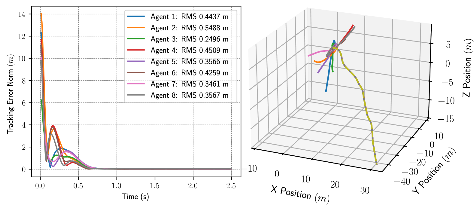
Figure 1: Left: Tracking error norm $\left\|e_{i}\right\|$ for $t\in\left[0,2.5\right]$s, showing cumulative RMS error of 0.3973m and convergence within 0.05m of target after 1.75s. Right: 3D agent trajectories for $t\in\left[0,15\right]$s.

A simulation is performed where a network of $N=8$ agents tracks a target agent with cycle graph topology and pinning matrix $B=\text{diag}\left\{1,0,1,0,1,0,1,0\right\}$. Initial agent positions are sampled from $U\left(-10,10\right)$ m, with zero initial velocities, while the target agent begins with velocity. $\left[\begin{array}[]{ccc}1&-1&0.5\end{array}\right]^{\top}$ $m/s$. Agent dynamics follow (1) with $f_{i}=\left[c_{i,1}\left(y_{i}-z_{i}\right)\right.+c_{i,2}\tanh\left(\dot{x}_{i}t\right)c_{i,3}\left(z_{i}-x_{i}\right)+c_{i,4}\tanh\left(\dot{y}_{i}t\right)c_{i,5}\left(x_{i}-y_{i}\right)+\left.c_{i,6}\tanh\left(\dot{z}_{i}t\right)\right]^{\top}$, $g_{i}=I_{3}-\text{diag}\left\{c_{i,7}\cos\left(t\right),c_{i,8}\sin\left(t\right),c_{i,9}\cos\left(t\right)\sin\left(t\right)\right\}$, and $d_{i}=\left[\begin{array}[]{ccc}c_{i,10}\cos\left(t\right)&c_{i,11}\sin\left(t\right)&c_{i,12}\cos\left(t\right)\sin\left(t\right)\end{array}\right]^{\top}$ with parameters $c_{i,j}$ sampled from $U\left(-0.5,0.5\right)$. Target agent dynamics follow $f_{0}=\left[\sin\left(x_{0}\right)\right.-\cos\left(y_{0}\dot{x}_{0}\right)\cos\left(z_{0}\dot{y}_{0}\right)-\sin\left(x_{0}\right)-\sin\left(y_{0}\dot{z}_{0}\right)-\left.\sin\left(z_{0}\right)\right]^{\top}$. Gaussian noise ($\mu=0$, $\sigma=0.001$m) affects position and velocity measurements. Control gains are $k_{1}=k_{2}=10$, $k_{3}=25$, and $k_{4}=50$. Fig. 1 shows the norm of the tracking error $\left\|e_{i}\right\|$ and the 3D trajectories over subsets of the 30-second simulation.

VII Conclusion

This work has presented a decentralized RISE-based control framework for multi-agent target tracking that achieves exponential convergence while requiring only local information exchange. The key innovation lies in the development of a controller and Lyapunov-based stability analysis which results from incorporating the interaction matrix directly into the Lyapunov function, eliminating the need for 2-hop communication present in previous approaches. The control development necessitated the development of a novel $P$-function construction technique that accommodates the interaction matrix while preserving the mathematical properties required for stability guarantees. The nonsmooth stability analysis established semi-global exponential convergence to the target agent state despite the presence of bounded disturbances with bounded derivatives.

Several directions for future research emerge from this work. The current approach assumes a fixed communication topology; extending the results to time-varying, switching, or directed topologies would enhance applicability to dynamic environments. Investigating performance under communication delays and packet losses would provide insights into robustness under realistic network conditions. Finally, integrating adaptive elements to estimate unknown disturbance bounds could further enhance practical implementation.

References

• [1] F. L. Lewis, H. Zhang, K. Hengster-Movric, and A. Das, Cooperative control of multi-agent systems: optimal and adaptive design approaches. Springer Science and Business Media, 2013.
• [2] W. Ren and Y. Cao, Distributed Coordination of Multi-agent Networks. Springer London, 2013.
• [3] C. Kwon and I. Hwang, “Sensing-based distributed state estimation for cooperative multiagent systems,” IEEE Trans. Autom. Control, vol. 64, no. 6, pp. 2368–2382, 2019.
• [4] Y. Mao, H. Jafarnejadsani, P. Zhao, E. Akyol, and N. Hovakimyan, “Novel stealthy attack and defense strategies for networked control systems,” IEEE Trans. Autom. Control, vol. 65, no. 9, pp. 3847–3862, 2020.
• [5] D. S. Drew, “Multi-agent systems for search and rescue applications,” Curr. Robot. Rep., vol. 2, no. 2, pp. 189–200, 2021.
• [6] O. Patil, A. Isaly, B. Xian, and W. E. Dixon, “Exponential stability with RISE controllers,” IEEE Control Syst. Lett., vol. 6, pp. 1592–1597, 2022.
• [7] O. S. Patil, K. Stubbs, P. Amy, and W. E. Dixon, “Exponential stability with RISE controllers for uncertain nonlinear systems with unknown time-varying state delays,” in Proc. IEEE Conf. Decis. Control, pp. 6431–6435, 2022.
• [8] O. S. Patil, R. Kamalapurkar, and W. E. Dixon, “Saturated RISE controllers with exponential stability guarantees: A projected dynamical systems approach,” IEEE Trans. Autom. Control, pp. 1–8, 2025.
• [9] J. R. Klotz, Z. Kan, J. M. Shea, E. L. Pasiliao, and W. E. Dixon, “Asymptotic synchronization of a leader-follower network of uncertain euler-lagrange systems,” IEEE Trans. Control Netw. Syst., vol. 2, no. 2, pp. 174–182, 2015.
• [10] X. Wang, J. Sun, Z. Wu, and Z. Li, “Robust integral of sign of error-based distributed flocking control of double-integrator multi-agent systems with a varying virtual leader,” Int. J. Robust Nonlinear Control, vol. 32, no. 1, pp. 286–303, 2022.
• [11] H.-X. Hu, G. Wen, X. Yu, Z.-G. Wu, and T. Huang, “Distributed stabilization of heterogeneous mass in uncertain strong-weak competition networks,” IEEE Trans. Syst. Man Cybern. Syst., vol. 52, no. 3, pp. 1755–1767, 2022.
• [12] B. E. Paden and S. S. Sastry, “A calculus for computing Filippov’s differential inclusion with application to the variable structure control of robot manipulators,” IEEE Trans. Circuits Syst., vol. 34, pp. 73–82, 1987.
• [13] D. Shevitz and B. Paden, “Lyapunov stability theory of nonsmooth systems,” IEEE Trans. Autom. Control, vol. 39 no. 9, pp. 1910–1914, 1994.
• [14] R. Kamalapurkar, J. A. Rosenfeld, J. Klotz, R. J. Downey, and W. E. Dixon, “Supporting lemmas for RISE-based control methods.” arXiv:1306.3432, 2014.
• [15] R. Kamalapurkar, W. E. Dixon, and A. Teel, “On reduction of differential inclusions and Lyapunov stability,” ESAIM: Control, Optim. Calc. of Var., vol. 26, no. 24, pp. 1–16, 2020.
• [16] K. Y. Pettersen, “Lyapunov sufficient conditions for uniform semiglobal exponential stability,” Automatica, vol. 78, pp. 97–102, 2017.
• [17] A. Loría and E. Panteley, “Uniform exponential stability of linear time-varying systems: revisited,” Syst. Control Lett., vol. 47, no. 1, pp. 13–24, 2002.