Inference and Learning of Nonlinear LFR State-space Models*

Abstract

Estimating the parameters of nonlinear block-oriented state-space models from input-output data typically involves solving a highly non-convex optimization problem, making it susceptible to poor local minima and slow convergence. This paper presents a computationally efficient initialization method for fully parametrizing nonlinear linear fractional representation (NL-LFR) models using periodic data. The approach first infers the latent variables and then estimates the model parameters, yielding initial estimates that serve as a starting point for further nonlinear optimization. The proposed method shows robustness against poor local minima, and achieves a twofold error reduction compared to the state-of-the-art on a challenging benchmark dataset.

I INTRODUCTION

The identification of nonlinear dynamical systems from input-output data is challenging for two main reasons: first, a suitable model structure must be selected to accurately represent the system’s behavior; second, its parameters must be estimated, which is typically achieved through nonlinear optimization. Since the choice of model structure directly influences the parameter estimation process, it is essential to find the right balance between model parsimony and its ability to capture complex nonlinear phenomena.

State-space models are particularly appealing for modeling nonlinear systems, as they provide an efficient framework while also serving as the foundation for many modern model-based control techniques. A well-known example is the polynomial nonlinear state-space (PNLSS) model [1], which separates the nonlinear dynamics into a linear time-invariant (LTI) component and a static nonlinearity. Additional structure can be incorporated by recognizing that nonlinearities typically appear locally, motivating the use of block-oriented models [2, 3]. Block-oriented models describe the interaction between LTI blocks and static nonlinearities, making them more interpretable while requiring fewer parameters than the more general PNLSS model. Popular examples include the Hammerstein, Wiener, and Wiener-Hammerstein models. The focus of this work, however, is on the nonlinear linear fractional representation (NL-LFR) model, which features a nonlinear feedback loop, essential for capturing amplitude-dependent resonant behavior in many mechanical systems. Any block-oriented model with a single static nonlinearity can be expressed in NL-LFR form, making it the most general model of this type. A schematic overview of the model structure is shown in Fig. 1.

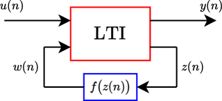
(a)

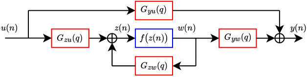
(b)

Figure 1: The NL-LFR model as (a) a multi-input, multi-output LTI block with nonlinear feedback, and (b) an equivalent interaction between LTI blocks and a static nonlinearity.

This paper focuses on NL-LFR simulation models, which, unlike finite-horizon prediction models, present greater parameter estimation challenges as the relationship between model parameters and simulated output becomes more nonlinear with increasing data length. Consequently, the optimization problem is highly non-convex, making it susceptible to poor local minima and potentially slow convergence due to the complexity of the loss landscape.

One approach to reducing the complexity of the estimation problem is to initialize the NL-LFR model with the best linear approximation (BLA) [4], which can be parametrized non-iteratively using subspace methods [5, 6]. For weakly nonlinear systems, this significantly simplifies the nonlinear optimization problem, as only deviations from the BLA need to be estimated. Another approach to reducing the complexity of parameter estimation is to first infer the model’s latent variables ($w$ and $z$ in Fig. 1), which removes recursive dependencies and hence facilitates a more tractable optimization problem. This strategy, known as inference and learning, is key to probabilistic methods such as the expectation-maximization algorithm [7, 8] and kernel-based methods leveraging canonical correlation analysis [9, 10]. Indeed, inference and learning can be combined with initialization strategies, as demonstrated in [11, 12, 13], leading to both higher accuracy and reduced training times.

Existing approaches for NL-LFR identification attempt to estimate the latent signals $w$ and $z$, but either rely on computationally expensive two-tone experiments [14], or require BLA estimates at multiple operating conditions [15]. Moreover, these methods are limited to cases where all five sub-blocks in Fig. 1 are single-input single-output (SISO) systems, significantly restricting the modeling flexibility of the NL-LFR structure. Other works focus on improving initialization rather than inferring internal signals. In [16], a fully nonlinear initialization approach is proposed for NL-LFR models, though it remains limited to the SISO case. Meanwhile, [17] imposes no restrictions on the dimensionality of the sub-blocks but relies solely on BLA-based initialization, which can still lead to slow convergence and suboptimal local minima.

This paper introduces a computationally efficient NL-LFR model identification method, combining BLA initialization with a novel frequency-domain inference and learning approach. The proposed method requires periodic data, and, as opposed to [14, 15, 16], allows for arbitrarily-sized sub-blocks, thus improving model flexibility. Compared to [17], we obtain a fully initialized NL-LFR model, aiming to mitigate the risk of poor local minima and accelerate subsequent nonlinear optimization. The remainder of this paper is structured as follows. Section II establishes the problem context, while Section III presents the proposed identification approach. Section IV demonstrates the method’s effectiveness on the parallel Wiener-Hammerstein benchmark dataset [18], and Section V concludes the paper.

Notation: The sets of real and complex numbers are denoted by $\mathbb{R}$ and $\mathbb{C}$, respectively, while $\mathbb{Z}_{>0}$ represents the set of positive integers. For a vector $x\in\mathbb{C}^{n}$ and a Hermitian, positive definite matrix $Q\in\mathbb{C}^{n\times n}$, the squared weighted 2-norm of $x$ is given by $\|x\|_{Q}^{2}=x^{\mathrm{H}}Qx$, where $x^{\mathrm{H}}$ denotes the conjugate transpose of $x$. For a real-valued vector $x\in\mathbb{R}^{n}$, the transpose is denoted by $x^{\top}$. The discrete Fourier transform (DFT) of the time-domain samples $\{x(n)\}_{n=0}^{N-1}$ at frequency index $k$ is expressed as $X(k)=\mathcal{F}_{d}\{x(n)\}$, while the inverse DFT at time instance $n$, for the frequency-domain samples $\{X(k)\}_{k=-N/2+1}^{N/2}$, is $x(n)=\mathcal{F}_{d}^{-1}\{X(k)\}$. Finally, the $n\times n$ identity matrix is denoted by $I_{n}$.

II PROBLEM STATEMENT

We begin by outlining the system class, model structure, and noise framework to define the problem setting.

Assumption 1 (System class).

The system to be identified is of the periodic in, same period out (PISPO) class, which contains systems where a periodic input produces a steady-state output with the same period.

Definition 1 (Model structure).

The considered NL-LFR model structure is parametrized as a discrete-time linear state-space representation interconnected with a static nonlinearity of polynomial form:

$$x(n+1) ={A}x(n)+{B}_{u}u(n)+B_{w}w(n),$$ (1a)

$$y_{0}(n) ={C_{y}}x(n)+D_{yu}u(n)+D_{yw}w(n),$$ (1b)

$$z(n) =C_{z}x(n)+D_{zu}u(n),$$ (1c)

$$w(n) =\beta^{\top}\phi({z}(n)),$$ (1d)

where $x(n)\in\mathbb{R}^{n_{x}}$ represents the latent state at time index $n$, and $u(n)\in\mathbb{R}^{n_{u}}$ and $y_{0}(n)\in\mathbb{R}^{n_{y}}$ are the observable system inputs and outputs, respectively, while $z(n)\in\mathbb{R}^{n_{z}}$ and $w(n)\in\mathbb{R}^{n_{w}}$ are the respective unobservable inputs and outputs of the static nonlinearity. The matrices $A\in\mathbb{R}^{n_{x}\times n_{x}}$, $B_{u}\in\mathbb{R}^{n_{x}\times n_{u}}$, $B_{w}\in\mathbb{R}^{n_{x}\times n_{w}}$, $C_{y}\in\mathbb{R}^{n_{y}\times n_{x}}$, $C_{z}\in\mathbb{R}^{n_{z}\times n_{x}}$, $D_{yu}\in\mathbb{R}^{n_{y}\times n_{u}}$, $D_{yw}\in\mathbb{R}^{n_{y}\times n_{w}}$, and $D_{zu}\in\mathbb{R}^{n_{z}\times n_{u}}$ constitute the to-be-estimated LTI parameters. The static nonlinearity is modeled through $\phi:\mathbb{R}^{n_{z}}\to\mathbb{R}^{n_{\phi}}$ and parameters $\beta\in\mathbb{R}^{n_{\phi}\times n_{w}}$. The function $\phi$ first applies a $\tanh$ operation element-wise to its input $z$, after which it maps the result to a feature vector of monomials, which may include cross-terms, up to a specified degree. The $\tanh$ operation can be seen as a well-behaved saturation function which ensures that the output elements of $\phi$ remain bounded.

Remark 1.

A direct feedthrough from $w(n)$ to $z(n)$ is not modeled, as this would result in an algebraic loop.

The output $y_{0}(n)$ is not directly observable due to the presence of measurement noise, formalized as follows.

Assumption 2 (Noise framework).

The output measurements are corrupted by zero-mean, possibly colored, stationary noise $v(n)$ with finite variance: $y(n)\coloneqq y_{0}(n)+v(n).$ The input $u(n)$ is assumed to be noiseless and exactly known.

Although the model (1) is defined in the time domain, certain optimization challenges can be mitigated by switching to the frequency domain. That is, the Fourier transform’s decoupling property can break recurrence in specific cases, thus simplifying the simulation process. To accommodate this, it is more natural to work with the block-oriented representation of Fig. 1, with LTI blocks:

$$G_{yu}(\zeta,\theta) =C_{y}(\zeta I_{n_{x}}-A)^{-1}B_{u}+D_{yu},$$ (2a)

$$G_{yw}(\zeta,\theta) =C_{y}(\zeta I_{n_{x}}-A)^{-1}B_{w}+D_{yw},$$ (2b)

$$G_{zu}(\zeta,\theta) =C_{z}(\zeta I_{n_{x}}-A)^{-1}B_{u}+D_{zu},$$ (2c)

$$G_{zw}(\zeta,\theta) =C_{z}(\zeta I_{n_{x}}-A)^{-1}B_{w},$$ (2d)

where $\zeta$ denotes the z-transform variable ($q$ in Fig. 1 represents the forward shift operator).

Remark 2.

The considered model structure is not unique; gains and delays can be exchanged between the different blocks without affecting the input-output behavior [14]. In addition, state-space similarity transformations can be applied, leading to infinitely many input-output equivalent representations, thus complicating parameter estimation.

The considered frequency-domain approach requires the excitation signals to be periodic, as formalized next.

Definition 2 (Random-phase multisine).

The input excitations are described by a random-phase multisine signal [4] with $N$ samples per period, where $N$ is even:

$${u}(n)\coloneqq\frac{2}{\sqrt{N}}\sum_{k=1}^{N/2-1}U_{k}\cos{(2\pi kf_{0}n+\varphi_{k})},$$ (3)

where $U_{k}$ denotes the excitation amplitude at frequency index $k$, and $f_{0}=f_{s}/N$ is the frequency resolution, with $f_{s}$ being the sampling frequency. The random phases $\varphi_{k}$ are independent and uniformly distributed on the interval $[0,2\pi)$.

In practice, $R$ independent realizations of (3) are used to estimate the model parameters, leading to dataset

$$\mathcal{D}=\big{\{}\big{(}u^{\left[r\right]}(n),y^{\left[r\right]}(n)\big{)}\big{\}}_{n=0,r=0}^{N-1,R-1}.$$ (4)

Some additional conditions on $\mathcal{D}$ are required to guarantee the validity or improve the quality of the model.

Assumption 3 (Steady state).

All signals in $\mathcal{D}$ are in steady state. In practice this is achieved by performing experiments with multiple consecutive periods of (3) and discarding the ones that contain transients.

Remark 3.

If multiple steady-state periods are available, $\mathcal{D}$ can be defined using the average of these periods, thereby improving the signal-to-noise ratio. Moreover, repeated periods allow for computation of the frequency-dependent estimate of the output noise variance [4], which can later serve as a weighting matrix in the estimation procedure.

Assumption 4 (Standardization).

To improve numerical stability and algorithm performance, the data in $\mathcal{D}$ are standardized to zero mean and unit variance.

To estimate the model parameters $\theta$, we formulate the following optimization problem:

$$\hat{\theta}=\arg\min_{\theta}V(\theta),\vskip-4.0pt$$ (5a)

where the frequency-domain loss function is given by

$$V(\theta)=\frac{1}{RN}\sum_{r=0}^{R-1}\sum_{k=0}^{N/2}\big{\|}Y^{\left[r\right]}(k)-\hat{Y}^{\left[r\right]}(k,\theta)\big{\|}_{\Lambda(k)}^{2},$$ (5b)

with $Y^{\left[r\right]}(k)$ denoting the DFT of $y^{\left[r\right]}(n)$, $\hat{Y}^{\left[r\right]}(k,\theta)$ the modeled output spectrum, and $\Lambda(k)$ a frequency-dependent weighting matrix. This work evaluates (5b) in two ways: initially, through an inference and learning approach, and subsequently, using a more conventional simulation method. In both cases, the optimization problem (5b) is solved using the Levenberg-Marquardt (LM) algorithm [19].

III METHOD

We estimate the model parameters in three sequential steps. First, in Section III-A, $\theta_{uy}=\{(A,B_{u},C_{y},D_{yu})\}$ is parametrized using the BLA. Second, in Section III-B, $\theta_{wz}=\{(B_{w},C_{z},D_{yw},D_{zu})\}$ and $\beta$ are parametrized through a frequency-domain inference and learning approach. Third, in Section III-C, all parameters $\theta=\{\theta_{uy},\theta_{wz},\beta\}$ are jointly optimized in simulation mode.

III-A Best linear approximation

Following [4], and given dataset $\mathcal{D}$, the BLA of a nonlinear system within the PISPO class is defined as:

$$\hat{G}(q)=\arg\min_{G}\mathbb{E}\left[\|y(n)-G(q)u(n)\|^{2}\right],$$ (6)

where $\mathbb{E}\left[\cdot\right]$ denotes the expected value operator. In this work, we estimate the BLA in the frequency domain using the DFT of the input-output data. The procedure consists of three steps. First, a nonparametric estimate of $\hat{G}$ is obtained (for details, see [4]). Second, $\hat{G}$ is parametrized, non-iteratively, in state-space form using the frequency-domain subspace method [6]. Third, the obtained parameters are refined through iterative LM optimization steps. The resulting matrices $\hat{A}$, $\hat{B}$, $\hat{C}$, and $\hat{D}$ are used to initialize:

$${\theta_{uy}}=\{(T_{x}^{-1}\hat{A}T_{x},\,\,T_{x}^{-1}\hat{B},\,\,\hat{C}T_{x},\,\,\hat{D})\},$$ (7)

where $T_{x}$ is a diagonal matrix containing the standard deviations of the BLA state simulations. This similarity transform scales the linear state trajectories to have unit variance, which is beneficial for the subsequent optimization steps.

III-B Full nonlinear initialization

The next step is to initialize all NL-LFR model parameters, which is achieved by solving (5b) with $\theta_{wz}\subseteq\theta$ as decision variables and $\theta_{uy}\subseteq\theta$ as static ones. The optimization scheme follows an inference and learning approach, where inference estimates the latent variables based on the observed data in $\mathcal{D}$ and the LTI parameters, and learning uses the inferred variables to efficiently estimate the coefficients $\beta$.

Before optimization, $\theta_{wz}$ is initialized using matrices $B_{w}^{*}$, $C_{z}^{*}$, $D_{yw}^{*}$, and $D_{zu}^{*}$, of which the elements are randomly sampled from a normal distribution with zero mean and unit variance. Specifically:

$${\theta}_{wz}=\{(B_{w}^{*},\,\,T_{z}^{-1}C_{z}^{*},\,\,{D}_{yw}^{*},\,\,T_{z}^{-1}D_{zu}^{*})\}.$$ (8)

For $C_{z}$ and $D_{zu}$ a scaling with diagonal matrix $T_{z}$ is applied, of which the diagonal elements are defined as $(z_{\max}^{*}-z_{\min}^{*})/2$. Here, $z_{\min}^{*},z_{\max}^{*}\in\mathbb{R}^{n_{z}}$ are the minimum and maximum values of the samples of $z^{*}$, respectively, where $z^{*}$ is obtained by simulating the BLA together with the initial values of $C_{z}^{*}$ and $D_{zu}^{*}$. This scaling approach ensures that the initial linear estimates of $z$ are within the range $[-1,1]$, thus providing a suitable input to the $\tanh$ function. In the following, $\tilde{\theta}=\{\theta_{uy},\theta_{wz}\}$, where $B_{w}^{*}$, $C_{z}^{*}$, $D_{yw}^{*}$, and $D_{yu}^{*}$ are iteratively optimized while the BLA is kept fixed.

III-B1 Inference of hidden variables

The objective of this step is to obtain estimates of the latent system variables. To do so, we formulate a frequency-domain optimization problem that minimizes $\mathcal{E}^{\left[r\right]}(k)={Y}^{\left[r\right]}(k)-\hat{Y}^{\left[r\right]}(k)$ while regularizing the required input $W^{\left[r\right]}(k)$:

$$\begin{split}\min_{{W}}\sum_{r=0}^{R-1}\sum_{k=0}^{N/2}\big{(}\frac{1}{2}\|\mathcal{E}^{\left[r\right]}(k)\|^{2}_{\Lambda(k)}+\frac{\lambda}{2}\|{W}^{\left[r\right]}(k)\|^{2}_{\Theta}&\big{)},\end{split}$$ (9a)

subject to

$$\hat{Y}^{\left[r\right]}(k)=G_{yu}(\zeta_{k},\tilde{\theta}){U}^{\left[r\right]}(k)+G_{yw}(\zeta_{k},\tilde{\theta}){W}^{\left[r\right]}(k),$$ (9b)

where $\zeta_{k}$ is the z-transform variable evaluated on the unit circle at DFT frequency $k$. The hyperparameter $\lambda>0$ controls solution variability by penalizing the influence of ${W}^{\left[r\right]}(k)$ on the state and output through

$$\Theta=\begin{bmatrix}B_{w}\\ D_{yw}\end{bmatrix}^{\top}\begin{bmatrix}B_{w}\\ D_{yw}\end{bmatrix}+\frac{\epsilon}{\lambda}I_{n_{w}},$$ (10)

where $\epsilon$ is a small positive value that guarantees strict positive definiteness of $\Theta$. Therefore, the optimization problem (9b) is convex, with closed-form solution:

$${W}_{*}^{\left[r\right]}(k)=\Omega^{-1}\Psi\big{(}{Y}^{\left[r\right]}(k)-G_{yu}(\zeta_{k},\tilde{\theta}){U}^{\left[r\right]}(k)\big{)},$$ (11)

where $\Psi=G^{\mathrm{H}}_{yw}(\zeta_{k},\tilde{\theta})\Lambda(k)$, and $\Omega=\Psi G_{yw}(\zeta_{k},\tilde{\theta})+\lambda\Theta$. Next, the corresponding estimate of ${Z}^{\left[r\right]}(k)$ is computed as

$${Z}_{*}^{\left[r\right]}(k)=G_{zu}(\zeta_{k},\tilde{\theta}){U}^{\left[r\right]}(k)+G_{zw}(\zeta_{k},\tilde{\theta}){W}_{*}^{\left[r\right]}(k),$$ (12)

which concludes the inference step.

III-B2 Learning of model parameters

The process of learning consists of three stages. First, the nonlinear model parameters $\beta$ are determined from the inferred signals by solving an estimation problem that is linear in the parameters. Second, an iterative root-finding algorithm is applied to promote consistent feedback dynamics. Third, the elements of $\theta_{wz}$ are iteratively adjusted to minimize the loss in (5b).

(i) Solving for $\beta$: Using the obtained nonparametric spectral estimates in (11) and (12), the coefficients $\beta$ can be learned by solving an estimation problem that is linear in the parameters. We perform this step in the time domain, since this significantly simplifies the construction of the nonlinear monomials. We define the relations:

$${\mathcal{W}}_{*}^{\left[r\right]} =\big{[}{w}_{*}^{\left[r\right]}(0),\ldots,{w}_{*}^{\left[r\right]}(N-1)\big{]}^{\top}\in\mathbb{R}^{N\times n_{w}},$$ (13a)

$$\mathcal{W}_{*} =\big{[}(\mathcal{W}_{*}^{\left[0\right]})^{\top},\ldots,(\mathcal{W}_{*}^{\left[R-1\right]})^{\top}\big{]}^{\top}\in\mathbb{R}^{(NR)\times n_{w}},$$ (13b)

$${\mathcal{Z}}_{*}^{\left[r\right]} =\big{[}{z}_{*}^{\left[r\right]}(0),\ldots,{z}_{*}^{\left[r\right]}(N-1)\big{]}^{\top}\in\mathbb{R}^{N\times n_{z}},$$ (13c)

$$\mathcal{Z}_{*} =\big{[}(\mathcal{Z}_{*}^{\left[0\right]})^{\top},\ldots,(\mathcal{Z}_{*}^{\left[R-1\right]})^{\top}\big{]}^{\top}\in\mathbb{R}^{(NR)\times n_{z}},$$ (13d)

where ${w}_{*}^{\left[r\right]}(n)$ and ${z}_{*}^{\left[r\right]}(n)$ are the inverse DFTs of (11) and (12), respectively. Equation (13) allows for writing the nonlinear relationship (1d) in matrix-form as $\mathcal{W}^{*}=\Phi({\mathcal{Z}_{*}})\beta$, where $\Phi:\mathbb{R}^{(NR)\times n_{z}}\to\mathbb{R}^{(NR)\times n_{\phi}}$ applies $\phi$ row-wise to its input. The estimation of $\beta$ then simplifies to:

$$\hat{\beta}=\big{(}\Phi^{\top}({\mathcal{Z}}_{*})\Phi({\mathcal{Z}}_{*})\big{)}^{-1}\Phi^{\top}({\mathcal{Z}}_{*})\mathcal{W}_{*},$$ (14)

which, together with $\tilde{\theta}$, fully defines the NL-LFR model.

(ii) Promoting internal consistency: A tempting approach to evaluating the loss function in (5b) is to directly use $\hat{\beta}$ and $z_{*}^{\left[r\right]}(n)$ to define the parametric estimate:

$${W}_{\beta}^{\left[r\right]}(k)=\mathcal{F}_{d}\big{\{}\hat{\beta}^{\top}\phi\big{(}{z}_{*}^{\left[r\right]}(n)\big{)}\big{\}},$$ (15)

which can be used to compute $\hat{Y}^{\left[r\right]}(k,\theta)$ in (5b). However, this approach ignores the feedback dynamics, as it does not account for the effect of ${W}_{\beta}^{\left[r\right]}(k)$ on itself through

$${Z}_{\beta}^{\left[r\right]}(k)=G_{zu}(\zeta_{k},\tilde{\theta}){U}^{\left[r\right]}(k)+G_{zw}(\zeta_{k},\tilde{\theta}){W}_{\beta}^{\left[r\right]}(k).$$ (16)

If the feedback dynamics were consistent, one could replace ${z}_{*}^{\left[r\right]}(n)$ in (15) with $\mathcal{F}_{d}^{-1}\{{Z}_{\beta}^{\left[r\right]}(k)\}$, and then recompute (16) without affecting the value of ${Z}_{\beta}^{\left[r\right]}(k)$. The problem, however, is that any practical estimate of $\hat{\beta}$ that imperfectly describes the relationship between the nonparametric signals $\mathcal{Z}_{*}$ and $\mathcal{W}_{*}$, does change the reconstructed ${Z}_{\beta}^{\left[r\right]}(k)$, and is therefore inconsistent. This inconsistency can become problematic when the NL-LFR model is simulated forward in time: the output $w$ of the nonlinear function $\phi$ at time $n$ affects its own input $z$ at time $n+1$. As a result, small inconsistencies no longer remain locally contained but instead accumulate over time, leading to a mismatch between the training and simulation environment that may quickly result in divergence [20].

The risk of divergence motivates the search for a parametric estimate of ${W}^{\left[r\right]}(k)$ that not only minimizes the loss in (5b), but also reduces internal inconsistency. To formalize this, we express the feedback dynamics (16) in implicit form:

$$Z_{\beta_{*}}^{\left[r\right]}(k)=\Gamma_{k}\big{(}Z_{\beta_{*}}^{\left[r\right]}(k)\big{)},$$ (17)

where $\Gamma_{k}:\mathbb{C}^{n_{z}}\to\mathbb{C}^{n_{z}}$ represents the implicit feedback mapping, of which a visual representation is given in Fig. 2. Equation (17) characterizes a consistent feedback loop, since applying $\Gamma_{k}$ to $Z_{\beta_{*}}^{\left[r\right]}(k)$ results in $Z_{\beta_{*}}^{\left[r\right]}(k)$ being reproduced. In other words, $Z_{\beta_{*}}^{\left[r\right]}(k)$ is what is known as a fixed point of $\Gamma_{k}$. This insight enables us to (i) define consistency in terms of fixed points, and (ii) search for such points based on the initial nonparametric estimate of $Z^{\left[r\right]}(k)$ in (12) and the obtained value of $\hat{\beta}$. This search is realized by iteratively looping through $\Gamma_{k}$, as formalized in the following definition.

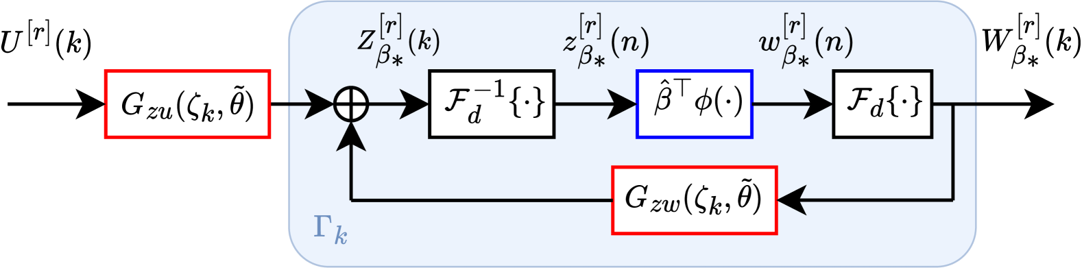
Figure 2: Schematic of a consistent feedback loop: ${Z}_{\beta_{*}}^{\left[r\right]}(k)$ is invariant to the feedback transformation $\Gamma_{k}$.

Definition 3 (Fixed-point iterations).

Given the initial nonparametric estimate ${Z}_{\beta_{0}}^{\left[r\right]}(k)={Z}_{*}^{\left[r\right]}(k)$, we perform $\tau\in\mathbb{Z}_{>0}$ fixed-point iterations according to:

$$\big{\{}{Z}_{\beta_{i+1}}^{\left[r\right]}(k)=\Gamma_{k}\big{(}{Z}_{\beta_{i}}^{\left[r\right]}(k)\big{)}\big{\}}_{i=0,r=0,k=0}^{\tau-1,R-1,N/2}.$$ (18)

By Banach’s fixed-point theorem, if $\Gamma_{k}$ is a contraction mapping, the sequence is guaranteed to converge to a unique fixed point for sufficiently large $\tau$.

Note that $\Gamma_{k}$ being contractive depends on the specific elements of $\tilde{\theta}$ and $\hat{\beta}$. Rather than enforcing contractiveness explicitly, we argue that the optimizer implicitly promotes this property by adjusting $\theta_{wz}$ during the optimization process. The effectiveness of the proposed fixed-point interations in terms of time-domain stability and performance is experimentally validated in Section IV.

Remark 4.

It is generally not required for ${Z}_{\beta_{\tau}}^{\left[r\right]}(k)$ to be an exact fixed point of $\Gamma_{k}$. Instead, it needs to be sufficiently close to ensure bounded and numerically stable time-domain simulations of the NL-LFR model.

(iii) Updating $\theta_{wz}$: From the final fixed-point iteration we compute the modeled output as

$$\hat{Y}^{\left[r\right]}(k,\theta)=G_{yu}(\zeta_{k},\tilde{\theta}){U}^{\left[r\right]}(k)+G_{yw}(\zeta_{k},\tilde{\theta}){W}_{\beta_{\tau}}^{\left[r\right]}(k),$$ (19)

where ${W}_{\beta_{\tau}}^{\left[r\right]}(k)=\mathcal{F}_{d}\big{\{}\hat{\beta}^{\top}\phi\big{(}\mathcal{F}_{d}^{-1}\{{Z}_{\beta_{\tau}}^{\left[r\right]}(k)\}\big{)}\big{\}}.$ Equation (19) is then used to evaluate the loss in (5b), where the decision variables $\theta_{wz}$ are iteratively adjusted until either convergence is achieved or the maximum number of iterations is reached. A complete overview of the proposed inference and learning approach is provided in Algorithm 1.

Algorithm 1 Inference and learning of NL-LFR models

1:Input: Dataset $\mathcal{D}$, BLA parameters $\theta_{uy}$, regularization parameter $\lambda$, and number of fixed-point iterations $\tau$

2:Initialize $\theta_{wz}$ using random values $\triangleright$ Eq. (8)

3:while not converged do

4:  1) Inference of hidden variables

5:  for $r=0$ to $R-1$ do

6:   for $k=0$ to $N/2$ do

7:     Compute ${W}_{*}^{\left[r\right]}(k),\>{Z}_{*}^{\left[r\right]}(k)$ $\triangleright$ Eqs. (11)–(12)

8:   end for

9:  end for

10:  2) Learning of model parameters

11:  (i) Solve a linear problem to obtain $\hat{\beta}$ $\triangleright$ Eq. (14)

12:  (ii) Perform $\tau$ fixed-point iterations $\triangleright$ Eq. (18)

13:  (iii) Update elements of $\theta_{wz}$ $\triangleright$ Eqs. (19) and (5b)

14:end while

15:Output: Fully initialized NL-LFR model

III-C Full nonlinear optimization

At this stage, all NL-LFR parameters have been initialized, i.e., $\theta=\{\tilde{\theta},\hat{\beta}\}$, but further optimization is needed to improve the simulation performance of the model. Therefore, we optimize all parameters $\theta$ using forward simulations driven by $u^{\left[r\right]}(n)$. We take the DFT of the simulated output to minimize the frequency-domain loss function (5b). It may be expected that poor local minima are avoided since the previous steps should have already provided a good initialization.

IV RESULTS

We evaluate the effectiveness of the proposed method on the parallel Wiener-Hammerstein benchmark system [18], where each of the two branches contains a diode-resistor static nonlinearity, sandwiched between two third-order linear filters. The overall SISO system exhibits 12th-order dynamics ($n_{x}=12$) and can be reformulated as an NL-LFR structure with a multi-input multi-output (MIMO) nonlinearity ($n_{w}=n_{z}=2$). The nonlinearity is modeled using monomial basis functions up to degree 7, including cross-terms, resulting in a total of 293 model parameters.

For estimation, we use $R=5$ realizations, each obtained by averaging two steady-state periods (see Remark 3) of random-phase multisines with with $N=16384$ samples and an RMS excitation amplitude of 1 V. All experiments are conducted on a Nvidia GeForce RTX 2080 Ti GPU. Implementation details are provided in this work’s repository.

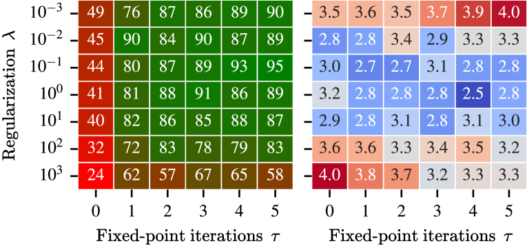
Figure 3: Impact of $\tau$ and $\lambda$ on the simulation stability of the inference and learning method, based on 100 random initializations per grid point: (left) number of runs that led to stable time-domain simulations; (right) corresponding average simulation error (expressed as a percentage).

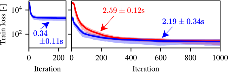
Figure 4: Training progress of 100 random initializations of $\theta_{wz}$: (left) inference and learning method for $\lambda=10^{0}$ and $\tau=3$; (right) full nonlinear optimization. Blue: proposed method; red: baseline method. The numbers indicate the computation time per iteration (mean $\pm$ standard deviation).

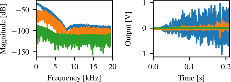
Figure 5: Simulations on test data: (left) multisine in frequency domain; (right) arrowhead in time domain. Blue: system output; orange: BLA error; green: NL-LFR error.

TABLE I: Comparison of simulation RMSEs (in volts) on the multisine and arrowhead test datasets.

	BLA	Proposed	ParWH [18]	NL-LFR [17]
Multisine	3.77e-2	6.04e-4	1.10e-3	1.37e-3
Arrowhead	4.54e-2	6.12e-4	2.66e-3	1.42e-3

First, we assess the effect of the number of fixed-point iterations $\tau$ and the regularization parameter $\lambda$ on the time-domain stability of the inference and learning method. Specifically, we perform a grid search over $\lambda\in\{10^{-3},10^{-2},\ldots,10^{3}\}$ and $\tau\in\{0,\ldots,5\}$. For each combination we run 250 LM iterations of inference and learning, and we repeat each trial 100 times with different random initializations of $\theta_{wz}$. The results are shown in Fig. 3, where the left grid indicates the number of trials that resulted in stable time-domain simulations; the right grid presents the corresponding mean relative simulation errors as percentages (for reference, the BLA error is 11.18%). Fig. 3 shows that the success rate generally increases with $\tau$, which aligns with expectations, as higher $\tau$ values enhance the model’s internal consistency and hence reduce accumulating time-domain errors. Moreover, the initialization method demonstrates robustness with respect to $\lambda$: a broad range of values leads to stable simulations with low errors; the performance only notably deteriorates at the extremes, both in terms of successful trials and simulation accuracy. In summary, inference and learning achieves a significant improvement over the BLA, and is generally stable across hyperparameters.

Next, we examine the impact of the inference and learning method on the final optimization stage. We do so by comparing the full proposed method to a baseline approach where the final optimization is initialized merely with the BLA. For the proposed method, we first perform 250 LM iterations of inference and learning with $\lambda=10^{0}$ and $\tau=3$, followed by 1000 LM iterations of nonlinear optimization. For the baseline approach, we directly perform 1000 LM iterations of nonlinear optimization. Both methods follow the same random initialization of $\theta_{wz}$ in (8), which is again repeated 100 times. For the baseline method, the elements of $\beta$ are initially set to zero, ensuring that the initial loss matches the BLA loss. Fig. 4 shows the median of the respective training loss progressions for all 100 trials, with shaded regions indicating the median absolute deviation. The left plot in Fig. 4 shows that inference and learning quickly reduces the training loss with with roughly a factor of 20, after which it plateaus, likely due to the optimizer’s degrees of freedom being restricted to $\theta_{wz}$ alone. From the right plot of Fig. 4 it can be seen that the obtained initial estimates provide a head start for the final optimization. As a result, the proposed method converges faster and to a slightly lower minimum compared to the baseline method. Notably, inference and learning produced 91 stable initializations, all of which converged to significantly lower local minima during final optimization. In contrast, only 85 trials of the baseline method showed significant improvement over the BLA, which suggests that starting farther from a good local minimum made them more prone to getting stuck in poor local minima. Fig. 4 also reports on the respective computational times per iteration, where, due to its parallelizable nature, the inference and learning iterations are over six times faster than those of the full nonlinear optimization. This efficiency enables rapid exploration of multiple model architectures, which is useful for practical applications.

Finally, from the trials in Fig. 4, we select the model with the lowest training loss and test it on two datasets: (i) another multisine realization with the same properties as the estimation data, and (ii) a Gaussian noise sequence with a linearly increasing amplitude over time (denoted as the arrowhead signal). The simulation results are shown in Fig. 5, where it is clear that the NL-LFR model significantly outperforms the BLA. The corresponding time-domain relative simulation errors are reduced from 11.29% to just 0.18% for the multisine data, and from 17.36% to 0.23% for the arrowhead signal. This improvement is also evident from Table I, where the proposed method is compared to the BLA and two state-of-the-art approaches: the first method explicitly enforces the parallel Wiener-Hammerstein structure [18], while the second initializes an NL-LFR model with the BLA and then models the residual [17] (similar to the baseline method). The selected model of this work outperforms both methods on both test datasets, achieving approximately a factor of two reduction in error, while requiring a similar number of parameters.

V CONCLUSIONS

This paper presented an inference and learning method for identifying NL-LFR state-space models. By combining initialization based on the BLA with the inference of latent variables and the learning of nonlinear parameters, the proposed method improves convergence properties and achieves the lowest error on a challenging benchmark dataset. Additionally, its computational efficiency allows for quickly exploring multiple model architectures, making it a promising tool for nonlinear system identification in practical applications. Future work will focus on extending the algorithm to non-periodic data and enhancing the performance of the inference and learning method by allowing the optimizer to also adjust the BLA parameters.

References

- [1] J. Paduart, L. Lauwers, J. Swevers, K. Smolders, J. Schoukens, and R. Pintelon, “Identification of nonlinear systems using polynomial nonlinear state space models,” Automatica, vol. 46, no. 4, 2010.
- [2] F. Giri and E.-W. Bai, Block-oriented nonlinear system identification. Springer, 2010, vol. 1.
- [3] M. Schoukens and K. Tiels, “Identification of block-oriented nonlinear systems starting from linear approximations: A survey,” Automatica, vol. 85, pp. 272–292, 2017.
- [4] R. Pintelon and J. Schoukens, System identification: a frequency domain approach. John Wiley & Sons, 2012.
- [5] P. Van Overschee and B. De Moor, “N4SID: Subspace algorithms for the identification of combined deterministic-stochastic systems,” Automatica, vol. 30, no. 1, pp. 75–93, 1994.
- [6] T. McKelvey, H. Akçay, and L. Ljung, “Subspace-based multivariable system identification from frequency response data,” IEEE Transactions on Automatic Control, vol. 41, no. 7, pp. 960–979, 1996.
- [7] R. Turner, M. Deisenroth, and C. Rasmussen, “State-space inference and learning with Gaussian processes,” in Proceedings of the Thirteenth International Conference on Artificial Intelligence and Statistics. JMLR Workshop and Conference Proceedings, 2010.
- [8] T. B. Schön, A. Wills, and B. Ninness, “System identification of nonlinear state-space models,” Automatica, vol. 47, no. 1, 2011.
- [9] V. Verdult, J. A. Suykens, J. Boets, I. Goethals, and B. De Moor, “Least squares support vector machines for kernel CCA in nonlinear state-space identification,” in Proceedings of the 16th International Symposium on Mathematical Theory of Networks and Systems (MTNS2004), Leuven, Belgium, 2004.
- [10] J.-W. van Wingerden and M. Verhaegen, “Closed-loop subspace identification of Hammerstein-Wiener models,” in Proceedings of the 48h IEEE Conference on Decision and Control (CDC) held jointly with 2009 28th Chinese Control Conference. IEEE, 2009, pp. 3637–3642.
- [11] A. Marconato, J. Sjöberg, J. A. Suykens, and J. Schoukens, “Improved initialization for nonlinear state-space modeling,” IEEE Transactions on Instrumentation and Measurement, vol. 63, no. 4, 2013.
- [12] M. Floren, S. Mamedov, J.-P. Noël, and J. Swevers, “Identification of Deformable Linear Object Dynamics from Input-output Measurements in 3D Space,” IFAC-PapersOnLine, vol. 58, no. 15, pp. 468–473, 2024.
- [13] M. Floren and J.-P. Noël, “Nonlinear restoring force modelling using Gaussian processes and model predictive control,” in Conference Proceedings of ISMA2022-USD2022, 2022, pp. 2493–2498.
- [14] G. Vandersteen and J. Schoukens, “Measurement and identification of nonlinear systems consisting of linear dynamic blocks and one static nonlinearity,” IEEE Transactions on Automatic Control, vol. 44, no. 6, pp. 1266–1271, 1999.
- [15] L. Vanbeylen, “Nonlinear LFR block-oriented model: Potential benefits and improved, user-friendly identification method,” IEEE Transactions on Instrumentation and Measurement, vol. 62, no. 12, 2013.
- [16] A. Van Mulders, J. Schoukens, and L. Vanbeylen, “Identification of systems with localised nonlinearity: From state-space to block-structured models,” Automatica, vol. 49, no. 5, pp. 1392–1396, 2013.
- [17] M. Schoukens and R. Tóth, “On the initialization of nonlinear LFR model identification with the best linear approximation,” IFAC-PapersOnLine, vol. 53, no. 2, pp. 310–315, 2020.
- [18] M. Schoukens, A. Marconato, R. Pintelon, G. Vandersteen, and Y. Rolain, “Parametric identification of parallel Wiener–Hammerstein systems,” Automatica, vol. 51, pp. 111–122, 2015.
- [19] K. Levenberg, “A method for the solution of certain non-linear problems in least squares,” Quarterly of applied mathematics, vol. 2, no. 2, pp. 164–168, 1944.
- [20] A. Venkatraman, M. Hebert, and J. Bagnell, “Improving multi-step prediction of learned time series models,” in Proceedings of the AAAI Conference on Artificial Intelligence, vol. 29, no. 1, 2015.