Effects of time-periodic drive in the linear response for planar-Hall set-ups with Weyl and multi-Weyl semimetals

Abstract

We investigate the influence of a time-periodic drive on three-dimensional Weyl and multi-Weyl semimetals in planar-Hall/planar-thermal-Hall set-ups. The drive is modelled here by circularly-polarized electromagnetic fields, whose effects are incorporated by a combination of the Floquet theorem and the van Vleck perturbation theory, applicable in the high-frequency limit. We evaluate the longitudinal and in-plane transverse components of the linear-response coefficients using the semiclassical Boltzmann formalism. We demonstrate the explicit expressions of these transport coefficients in certain limits of the system parameters, where it is possible to derive the explicit analytical expressions. Our results demonstrate that the topological charges of the corresponding semimetals etch their trademark signatures in these transport properties, which can be observed in experiments.

I Introduction

In contemporary reserach involving solid-state materials, there has been an upsurge in the explorations of systems exhibiting band-crossing points in the Brillouin zone, where the densities-of-states go to zero. These include the celebrated Weyl semimetals (WSMs)[1] and its cousins, the multi-Weyl semimetals (mWSMs) [2]. These are three-dimensional (3d) semimetals hosting nodal points, which also harbour nontrivial topological properties in their bandstructures. The topology of the 3d manifold formed by the Brillouin zone is responsible for giving rise to various novel properties. Fermi arcs, chiral anomaly, planar-Hall effects exemplify some such exotic characteristics. The nodal points behave as sinks and sources of the Berry flux, i.e., they act like the monopoles of the Berry curvature (BC) vector field, which arises from the Berry phase. Since the total topological charge over the entire Brillouin zone must vanish, these nodes must come in pairs, each pair carrying positive and negative topological charges of equal magnitude. This also follows from the Nielsen–Ninomiya theorem [3]. Mathematically, these monolpoles (or topological charges) are equivalent to the Chern numbers. The sign of the monopole charge is often referred to as the chirality of the corresponding node. While WSMs have a linear and isotropic dispersion and their band-crossing points harbour Chern numbers equalling $\pm 1$, mWSMs exhibit anisotropic dispersions, which turn out to be a hybrid of linear and nonlinear (in momentum) [cf. Fig. 1(a)]. The mWSMs, additionally, harbour nodes with Chern numbers $\pm 2$ (double-Weyl) or $\pm 3$ (triple-Weyl). It can be proved mathematically that the magnitude of the Chern number in mWSMs is bounded by $3$, by using symmetry arguments for crystalline structures [4, 5, 2]. Due to the nonzero topological charges of these systems, novel optical and transport properties, such as circular photogalvanic effect [6], circular dichroism [7], negative magnetoresistance [8, 9], and planar-Hall effect (PHE) [10], magneto-optical conductivity [11, 12, 13, 14] can emerge.

There has been unprecedented advancement in the experimental fronts as well, where WSMs have been realized experimentally [15, 16, 9, 17, 18] in compounds like TaA, NbA, and TaP. These materials have been reported to have topological charges equal to $\pm 1$. Compounds like $\text{HgCr}_{2}\text{Se}_{4}$ and $\text{SrSi}_{2}$ have been predicted to harbour double-Weyl nodes [4, 2, 19]. DFT calculations have found that nodal points in compounds of the form $\text{A(MoX)}_{3}$ (where A = Na, K, Rb, In, Tl, and X=S, Se, Te) have Chern numbers $\pm 3$ [20]. Dynamical/nonequilibrium topological semimetallic phases can also be designed by Floquet engineering [21, 22, 23, 24].

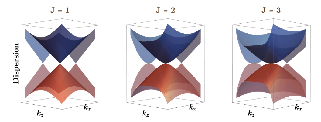
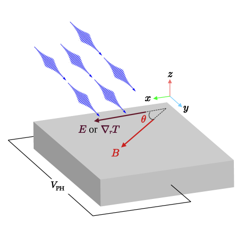
Figure 1: (a) Dispersion characteristics of a single node in a Weyl, double-Weyl, and triple-Weyl semimetal, respectively,plotted against the $k_{z}k_{x}$-plane. The double(triple)-Weyl node shows an anisotropic hybrid dispersion with a quadratic(cubic)-in-momentum dependence along the $k_{x}$-direction. In order to pinpoint the direction-dependent features, the projections of the dispersion along the respective momentum axes are also shown. (b) Schematics showing the planar-Hall (or planar-thermal Hall) experimental configuration, where the sample is subjected to a uniform electric field $E\,{\boldsymbol{\hat{x}}}$ (and/or a temperature gradient $\partial_{x}T\,{\boldsymbol{\hat{x}}}$) along the $x$-axis. An external magnetic field $\boldsymbol{B}$ is applied as well, which makes an angle $\theta$ with the $x$-axis. The blue wave-packets represent a time-periodic drive implemented by shining circularly polarized light.

When a conductor is placed in a magnetic field $\boldsymbol{B}$, such that it has a nonzero component perpendicular to the electric field $\boldsymbol{E}$ (which has been applied across the conductor), a current is generated perpendicular to the $\boldsymbol{E}$-$\boldsymbol{B}$ plane. This current is usually referred to as the Hall current, and the phenomenon is the well-known Hall effect. A generalization of this phenomenon is the PHE [10], when there is the emergence of a voltage difference perpendicular to an applied external $\boldsymbol{E}$, which is in the plane along which $\boldsymbol{E}$ and $\boldsymbol{B}$ lie [cf. Fig. 1(b)]. The planar-Hall conductivity, denoted by $\sigma_{xy}$ in this paper, is dependent on the angle between $\boldsymbol{E}$ and $\boldsymbol{B}$. In contrast with the canonical Hall conductivity, PHE does not require a nonzero component of $\boldsymbol{B}$ perpendicular to $\boldsymbol{E}$. While this novel phenomenon has been known to be found in ferromagnetic materials [25, 26, 27, 28, 29], they have been found to exist in semimetals which harbour nontrivial topology in their Brillouin zone. In particular WSMs/mWSMs possess a nontrivial BC, which source the so-called chiral anomaly [30, 31, 32, 33]. We would like to emphasize that the planar-Hall effect survives in a configuration in which the conventional Hall effect vanishes (because $\boldsymbol{E}$, $\boldsymbol{B}$, and the induced transverse Hall voltage, all lie in the same plane). Similar to the PHE, the planar thermal Hall effect [also referred to as the the planar Nernst effect (PNE)] is the appearance of a voltage gradient perpendicular to an applied temperature ($T$) gradient $\nabla_{\boldsymbol{r}}T$, which is coplanar with an externally applied magnetic field $\boldsymbol{B}$ [cf. Fig. 1(b)].

There have been extensive theoretical [34, 35, 36, 37, 38] and experimental [9, 39] studies of the transport coefficients in these planar Hall set-ups for various semimetals. Examples include longitudinal magneto-conductivity (LMC), planar Hall conductivity (PHC), longitudinal thermoelectric coefficient (LTEC), transverse thermoelectric coefficient (TTEC) (also known as the Peltier coefficient), and the components of the thermal conductivity. In this paper, we will compute these linear-response transport coefficients for WSMs and mWSMs, where such a semimetal is subjected to a time-periodic drive (for example, by shining circularly polarized light with frequency $\omega$). We will use the semiclassical Boltzmann approach for calculating these properties.

A widely used approach to analyze periodically driven systems, where the time-independent Hamiltonian is perturbed with a periodic potential, is the application of Floquet formalism [40, 37, 41, 42, 43, 44, 45]. The approach relies on the fact that a particle can gain or lose energy in multiples of $\hbar\omega$ (quantum of a photon), where $\omega$ is the driving frequency. Since the time($t$)-dependent Hamiltonian $H$ satisfies $H(t+\mathcal{T})=H(t)$, where $\mathcal{T}=2\,\pi/\omega$, we perform a Fourier transformation in tiem domain. When $\omega$ is much larger than the typical energy-bandwidth of the system, we can combine the Floquet formalism with the van Vleck perturbation theory to obtain an effective perturbative potential of the following form [40]:

$$V_{\text{eff}} =\sum\limits_{n=1}^{\infty}\left(\frac{\left[H_{-n},H_{n}\right]}{n\,\omega}+\frac{\left[\left[H_{-n},H_{0}\right],H_{n}\right]}{n^{2}\,\omega^{2}}+\cdots\right).$$ (1)

Here, $H_{\tilde{n}}$ denotes the ${\tilde{n}}^{\rm{th}}$ Fourier mode of the Hamiltonian.

The paper is organized as follows: In Sec. II, we explain the forms of the low-energy effective Hamiltonians for the WSMs and mWSMs. There, we also chalk out the formalism employed to compute the transport coefficiants in the planar-Hall set-ups, coupled with the application of a time-periodic drive. In Sec. III, we derive the explicit expressions for the in-plane components of the magneto-electric conductivity, dubbed as the LMC and the PHC. In Sec. III.4, we discuss the distinct characteristics observed from our results. Finally, we conclude with a summary and outlook in Sec. IV. The appendix contains some details regarding the explanations of the intermediate steps. In all our expressions, we will be using the natural units, which amounts to setting the reduced Planck’s constant ($\hbar$), the speed of light ($c$), and the Boltzmann constant ($k_{B}$) to unity. Additionally, electric charge has no units, with the magnitude of a single electronic charge measuring $e=1$. Nevertheless, we will retain the symbol $e$ in our linear-response tensors purely for the purpose of bookkeeping.

II Model and formalism

The low-energy effective Hamiltonian in the vicinity of a single WSM/mWSM node, with topological charge $J$, can be written as [4, 2, 5]

$$H_{J}\left(\boldsymbol{k}\right)=\boldsymbol{d}_{\boldsymbol{k}}\cdot\boldsymbol{\sigma}=\begin{bmatrix}v_{z}\,k_{z}&\alpha_{J}\left(k_{x}-i\,k_{y}\right)^{J}\\ \alpha_{J}\left(k_{x}+i\,k_{y}\right)^{J}&-\,v_{z}\,k_{z}\end{bmatrix},\text{ with }J\in(1,2,3),$$

$$\boldsymbol{d}_{\boldsymbol{k}}=\left\{\alpha_{J}\,k^{J}_{\perp}\cos\left(J\,\phi_{k}\right),\,\alpha_{J}\,k^{J}_{\perp}\sin\left(J\,\phi_{k}\right),\,v_{z}\,k_{z}\right\},\quad k_{\perp}=\sqrt{k_{x}^{2}+k_{y}^{2}}\,,\quad\phi_{k}=\arctan\Big(\frac{k_{y}}{k_{x}}\Big{missing})\,,\quad\alpha_{J}=\frac{v_{\perp}}{k_{0}^{J-1}}\,.$$ (2)

Here, $v_{z}$ and $v_{\perp}$ are the Fermi velocities in the $z$-direction and $xy$-plane, respectively, and $k_{0}$ is a system-dependent parameter with the dimension of momentum. The vector $\boldsymbol{\sigma}$ comprises the three Pauli matrices (viz. $\sigma_{x}$, $\sigma_{y}$, and $\sigma_{z}$), defining the pseudospin space. The value of $J=1$ represents the WSM, which has a linear and isotropic dispersion with $v_{\perp}=v_{z}$. The energy eigenvalues are given by $(-1)^{m}\,\epsilon^{(0)}_{\boldsymbol{k}}$, where

$$\epsilon^{(0)}_{\boldsymbol{k}}=\sqrt{\alpha^{2}_{J}\,k^{2J}_{\perp}+v_{z}^{2}\,k^{2}_{z}}\;\text{ and }m\in(0,1)\,,$$ (3)

with the values “$0$” and “$1$” representing the conduction and valence bands, respectively. The hybrid nature of the dispersion for $J>1$ is depicted in Fig. 1(a).

The quasiparticle-velocity (or group-velocity) vectors, associated with the conduction and valence bands, are given by $(-1)^{m}\,{\boldsymbol{v}}^{(0)}$, where

$${\boldsymbol{v}}^{(0)}\equiv\left\{v^{(0)}_{x},\,v^{(0)}_{y},\,v^{(0)}_{z}\right\}={\nabla}_{\boldsymbol{k}}\epsilon^{(0)}_{\boldsymbol{k}}=\frac{1}{\epsilon^{(0)}_{\boldsymbol{k}}}\left\{J\,k_{x}\,\alpha_{J}^{2}\,k_{\perp}^{2\,J-2},\,J\,k_{y}\,\alpha_{J}^{2}\,k_{\perp}^{2\,J-2},\,v_{z}^{2}\,k_{z}\right\}.$$ (4)

The $i^{\rm{th}}$-component of the BC for the $m^{\textrm{th}}$ band is given by [46]

$$\boldsymbol{\Omega}^{(m)}_{i}(\boldsymbol{k}) =\frac{(-1)^{m}\,\epsilon_{ijl}}{4}\,\frac{\boldsymbol{d}_{\boldsymbol{k}}\cdot\left(\partial_{k_{j}}\boldsymbol{d}_{\boldsymbol{k}}\times\partial_{k_{l}}\boldsymbol{d}_{\boldsymbol{k}}\right)}{|\boldsymbol{d}_{\boldsymbol{k}}|^{3}}\,,\text{ with }i,\,j,\,l\in\{x,y,z\}$$

$$\Rightarrow\boldsymbol{\Omega}^{(m)}(\boldsymbol{k}) =\frac{(-1)^{m}\,J\,v_{z}\,\alpha_{J}^{2}\,k^{2J-2}_{\perp}}{2\,\left(\epsilon^{(0)}_{\boldsymbol{k}}\right)^{3}}\left\{k_{x},\,k_{y},\,J\,k_{z}\right\}.$$ (5)

Clearly, the components of ${\boldsymbol{\Omega}}^{m}(\boldsymbol{k})$ are anisotropic for $J>1$. We have chosen the convention such that the chirality (and, hence, the Chern number) is positive for the conduction band, taking the explicit form of ${\boldsymbol{\Omega}}^{(0)}(\boldsymbol{k})=\frac{J\,v_{z}\,\alpha_{J}^{2}\,k^{2J-2}_{\perp}}{2\,\left(\epsilon^{(0)}_{\boldsymbol{k}}\right)^{3}}\left\{k_{x},\,k_{y},\,J\,k_{z}\right\}.$ In the following, we will consider the case when the chemical potential $\mu$ (measured with respect to the nodal point) cuts the positive-energy band (i.e., $\mu>0$).

II.1 Semiclassical Boltzmann formalism

In this subsection, we will review the semiclassical Boltzmann formalism [47, 48, 49, 50], which is used to calculate the transport coefficients in the set-ups shown in Fig. 1(b). In particular, we limit ourselves to the regime when the externally-applied magnetic field ($\boldsymbol{B}$) has a small-enough magnitude, leading to a small cyclotron frequency $\omega_{c}=e\,B/m^{*}$ (where $m^{*}$ is the effective mass with the magnitude $\sim 0.11\,m_{e}$, with $m_{e}$ denoting the electron mass), which satisfies $\omega_{c}\ll\mu$. This condition ensures that we can ignore the quantization of the dispersion into the form of Landau levels. While the details of the step-by-step derivations of the linear-response tensors can be found in Refs. [49, 50] in the context of nodal-point semimetals, we summarize the salient points here. When we use the Boltzmann equations to describe the evolution of the distribution function $f(\boldsymbol{k},\boldsymbol{r},t)$ of fermionic quasiparticles, we start with the form given by

$$\left(\frac{\partial}{\partial t}+\,\dot{\boldsymbol{r}}\,.{\nabla}_{\boldsymbol{r}}+\,\dot{\boldsymbol{k}}\,.{\nabla}_{\boldsymbol{k}}\right)f(\boldsymbol{k},\boldsymbol{r},t)=I_{coll}[{f(\boldsymbol{k},\boldsymbol{r},t)}]\,,$$ (6)

which results from the Liouville’s equation in the presence of scattering events. The term on the right-hand side (viz. $I_{coll}[{f(\boldsymbol{k},\boldsymbol{r},t)}]$) represents the collision integral, and arises due to scattering of electrons (e.g., scattering from lattice or from impurities). In the relaxation-time approximation, $I_{coll}[{f(\boldsymbol{k},\boldsymbol{r},t)}]$ is approximated as $\delta f/\tau$, where (1) $\delta f=f_{0}-f$, (2) $\tau$ is known as the relaxation time, and (3) $f_{0}$ is the equilibrium value of $f$ (i.e., in the absence of any externally applied fields), captured by the Fermi-Dirac distribution function. Physically, $\tau$ is a phenomenological estimate of the average time between successive collisions of the quasiparticles. For the fermionic quasiparticles occupying a band with the dispersion represented as $\varepsilon(\boldsymbol{k})$, $f_{0}=f_{0}(\varepsilon(\boldsymbol{k}),\mu,T)\equiv\left[1+e^{\frac{\varepsilon(\boldsymbol{k})-\mu}{T}}\right]^{-1}$.

Here, we are interested in looking for steady-state solutions, for which $f(\boldsymbol{k},\boldsymbol{r},t)$ is time-independent, implying $f(\boldsymbol{k},\boldsymbol{r},t)=f(\boldsymbol{k},\boldsymbol{r})$. Under these circumstance, Eq. (7) reduces to

$$\left(\dot{\boldsymbol{r}}\cdot{\nabla}_{\boldsymbol{r}}+\dot{\boldsymbol{k}}\cdot{\nabla}_{\boldsymbol{k}}\right)f({\boldsymbol{k}},\boldsymbol{r})=\frac{-\,\delta f({\boldsymbol{k}},\boldsymbol{r})}{\tau}\,.$$ (7)

For a system harbouring a nontrivial BC [51, 52, 50, 49], which we denote by ${\boldsymbol{\Omega}}_{F}$, under the effect of a magnetic field $\boldsymbol{B}$, it is necessary to introduce a phase-space factor defined by

$$\mathcal{D}({\boldsymbol{k}}) =\left[1+e\;\boldsymbol{B}\cdot{\boldsymbol{\Omega}}_{F}({\boldsymbol{k}})\right]^{-1},$$ (8)

which ensures that the Liouville’s theorem continues to hold in equilibrium (i.e., in the absence of any external probe fields). More specifically, ${\mathcal{D}}({\boldsymbol{k}})$ arises from the fact that ${\boldsymbol{\Omega}}_{F}({\boldsymbol{k}})$ modifies the phase-space volume element as $d^{3}\boldsymbol{k}\,d^{3}\boldsymbol{x}\rightarrow d^{3}\boldsymbol{k}\,d^{3}\boldsymbol{x}\,\mathcal{D}^{-1}({\boldsymbol{k}})$. After incorporating this correction, the final forms of the semiclassical transport equations for a system with BC turn out to be

$$\dot{\boldsymbol{r}} =\mathcal{D}\left[\boldsymbol{v}+e\left(\boldsymbol{E}\times{\boldsymbol{\Omega}}_{F}\right)+e\left(\boldsymbol{v}\cdot{\boldsymbol{\Omega}}_{F}\right)\boldsymbol{B}\right]\,,\quad\dot{\boldsymbol{k}}=-\mathcal{D}\left[e\,\boldsymbol{E}+e\left(\boldsymbol{v}\times\boldsymbol{B}\right)+e^{2}\left(\boldsymbol{E}\cdot\boldsymbol{B}\right){\boldsymbol{\Omega}}_{F}\right].$$ (9)

Here, $\boldsymbol{v}$ denotes the quasiparticles’ group velocity. Incorporating all these ingredients, Eq. (7) reduces to

$$\mathcal{D}\,\left[\left\{\boldsymbol{v}+e\,{\boldsymbol{E}}\crossproduct\boldsymbol{\Omega}_{F}+e\left({\boldsymbol{\Omega}}_{F}\cdot\boldsymbol{v}\right)\boldsymbol{B}\right\}\cdot\nabla_{\boldsymbol{r}}-e\left({\boldsymbol{E}}+\boldsymbol{v}\crossproduct{\boldsymbol{B}}\right)\cdot\nabla_{\boldsymbol{k}}-e^{2}\left({\boldsymbol{E}}\cdot{\boldsymbol{B}}\right)\,{\boldsymbol{\Omega}}_{F}\cdot\nabla_{\boldsymbol{k}}\right]f=\frac{-\,\delta f}{\tau}\,.$$ (10)

Next, one assumes that the probe fields, viz., $\boldsymbol{E}$, $\nabla_{\boldsymbol{r}}T$, and the resulting $\delta f$, are of the same order of smallness. To the leading order in this “smallness parameter”, the so-called linearized Boltzmann equation is obtained as

$$-e\left[\left\{{\boldsymbol{v}}+e\left({\boldsymbol{\Omega}}_{F}\cdot{\boldsymbol{v}}\right)\boldsymbol{B}\right\}\cdot\boldsymbol{E}\right]\frac{\partial f_{0}(\varepsilon,\mu,T)}{\partial\varepsilon}+e\,{\boldsymbol{B}}\cdot\left({\boldsymbol{v}}\crossproduct\nabla_{\boldsymbol{k}}\right)\,\delta f=-\frac{\delta f}{\tau\,\mathcal{D}}\,.$$ (11)

Now, the charge- and thermal-current densities are given by [47, 48, 49]

$$J^{i} =\sigma_{ij}\,E^{j}+\alpha_{ij}\,(-{\nabla}_{r_{j}}T)\,,\quad J^{Q}_{i}=T\,\alpha_{ij}\,E^{j}+\ell_{ij}\,(-{\nabla}_{r_{j}}T)\,,$$ (12)

respectively. Here, $\sigma_{ij}$ and $\alpha_{ij}$ define the components of the electric-conductivity tensor and the thermoelectric coefficients, respectively. The third one, namely $\ell$, is the tensor relating the thermal-current density to the temperature gradient at a vanishing electric field. Since $\ell$ contributes to the magnetothermal conductivity tensor, we will loosely refer to $\ell_{ij}$ themselves as the magnetothermal coefficients.

For investigating the response in the planar-Hall and planar-thermal-Hall set-ups, we consider the application of an external electric field $\boldsymbol{E}$ and/or temperature gradient along the $x$-axis [viz. $\boldsymbol{E}=E\,\boldsymbol{{\hat{x}}}$ and $\nabla_{\boldsymbol{r}}=\partial_{x}T\,\boldsymbol{{\hat{x}}}$], accompanied by an external magnetic field $\boldsymbol{B}$ along the $xy$-plane [viz., $\boldsymbol{B}=B_{x}\,\boldsymbol{{\hat{x}}}+B_{y}\,\boldsymbol{{\hat{y}}}$]. We will denote the angle made by $\boldsymbol{B}$ with respect to the $x$-axis as $\theta$, such that $B_{x}=B\cos\theta$ and $B_{y}=B\sin\theta$. Now the charge- and thermal-current densities are given by

$${\boldsymbol{J}} =-\,e\,\int\frac{d^{3}\boldsymbol{k}}{(2\,\pi)^{3}}\,\mathcal{D}^{-1}\,\dot{\boldsymbol{r}}\,f(\boldsymbol{r},\boldsymbol{k})\,,\text{ and }{\boldsymbol{J}}^{Q}=\int\frac{d^{3}\mathbf{k}}{(2\,\pi)^{3}}\,\mathcal{D}^{-1}\,\dot{\bf r}\,\left(\varepsilon-\mu\right)f(\bf r,\bf k)\,,$$ (13)

respectively, where $f$ is determined as the solution of Eq. (11). In particular, we will focus on the behaviour of the in-plane components (i.e., the $xx$- and $yx$-components) of the linear-response tensors, which are obtained by evaluating [53, 54]

$$\sigma_{ij}\approx-\,e^{2}\,\tau\int\frac{d^{3}\boldsymbol{k}}{(2\,\pi)^{3}}\,{\mathcal{D}}\left[v_{i}+e\,B_{i}\left({\boldsymbol{v}}\cdot\boldsymbol{\Omega}_{F}\right)\right]\left[v_{j}+e\,B_{j}\left({\boldsymbol{v}}\cdot\boldsymbol{\Omega}_{F}\right)\right]\,\frac{\partial f_{0}}{\partial\varepsilon}\,,$$

$$\alpha_{ij}\approx e\,\tau\int\frac{d^{3}\boldsymbol{k}}{(2\,\pi)^{3}}\,\mathcal{D}\left[v_{i}+e\,B_{i}\left({\boldsymbol{v}}\cdot\boldsymbol{\Omega}_{F}\right)\right]\left[v_{j}+e\,B_{j}\left({\boldsymbol{v}}_{s}\cdot\boldsymbol{\Omega}_{F}\right)\right]\,\frac{\left(\varepsilon-\mu\right)}{T}\,\frac{\partial f_{0}}{\partial\varepsilon}\,,$$

$$\ell_{ij}\approx-\,\tau\int\frac{d^{3}\boldsymbol{k}}{(2\,\pi)^{3}}\,\mathcal{D}\left[v_{i}+e\,B_{i}\left({\boldsymbol{v}}\cdot\boldsymbol{\Omega}_{F}\right)\right]\left[v_{j}+e\,B_{j}\left({\boldsymbol{v}}_{s}\cdot\boldsymbol{\Omega}_{F}\right)\right]\,\frac{\left(\varepsilon-\mu\right)^{2}}{T}\,\frac{\partial f_{0}}{\partial\varepsilon}\,.$$ (14)

We have used an “approximately equal to” ($\approx$) sign because we have ignored the contribution from the Lorentz-force factors arising from external magnetic field [i.e., from the part $e\,{\boldsymbol{B}}\cdot\left({\boldsymbol{v}}\crossproduct\nabla_{\boldsymbol{k}}\right)\,\delta f$ in Eq. (12)]. This is justified because these correction factors go to zero at leading order in the Lorentz-force operator, $\check{L}\equiv(\boldsymbol{v}\crossproduct\boldsymbol{B})\cdot\nabla_{\boldsymbol{k}}$, when we consider the in-plane components of the response tensors [54, 55, 56].

A few important observations and comments are in order. We would like to point out that the phase-space factor of $\mathcal{D}$ in the expression for $\alpha_{ij}$ was missed in Ref. [35] [cf. Eqs. (17) and (18) therein]. This, in some way, affected our computations in Ref. [57] (since we started with the erroneous expression of Ref. [35]), which we have self-retracted after realizing the mistake.

II.2 Time-periodic drive with a high frequency

On top of the applied electric and magnetic fields ($\boldsymbol{E}$ and $\boldsymbol{B}$), which are assumed to be static and uniform, we subject the system to a time-periodic optical drive with high value of frequency, $\omega$. While the corresponding electric-field vector for the light waves can be represented as ${\boldsymbol{\mathcal{E}}}(t)=E_{0}\left[-\cos(\omega t)\,\boldsymbol{{\hat{x}}}+\sin(\omega\,t)\,\boldsymbol{{\hat{y}}}\right]$, a vector potential for the associated magnetic field can be written as ${\boldsymbol{A}}(t)=\frac{E_{0}}{\omega}\left[\sin(\omega\,t)\,\boldsymbol{{\hat{x}}}+\cos(\omega\,t)\,\boldsymbol{{\hat{y}}}\right]$ upon using the Landau gauge. The effect of the circularly polarized electromagnetic field on the Hamiltonian $H_{J}$ can be obtained via the Peierls substitution, $\boldsymbol{k}\rightarrow\boldsymbol{k}-e\,\boldsymbol{A}$. Defining $A_{0}=\frac{e\,E_{0}}{\omega}$, the gauge-dependent momentum components are found via $k_{x}\rightarrow k_{x}^{\prime}=k_{x}-A_{0}\sin(\omega\,t)$, $k_{y}\rightarrow k_{y}^{\prime}=k_{y}-A_{0}\cos(\omega\,t)$, and $k_{z}\rightarrow k_{z}^{\prime}=k_{z}$. Using the binomial expansion, we obtain $(k^{\prime}_{x}\,\pm\,i\,k^{\prime}_{y})^{J}=\sum\limits_{m=0}^{J}(k_{\perp}\,e^{\pm i\,\phi_{k}})^{J-m}\,(-A_{0})^{m}\,e^{\pm i\,m\,(\frac{\pi}{2}-\omega\,t)}~{}^{J}C_{m}$, where $~{}^{J}C_{m}=\frac{J!}{(J-m)!\,m!}$ represents the combinatorial factor. With these ingredients, the resulting time-dependent Hamiltonian takes the form of

$$\tilde{H}_{J}({\boldsymbol{k}},{\boldsymbol{A}}) =\left[\alpha_{J}\left(k^{\prime}_{x}-i\,k^{\prime}_{y}\right)^{J}\sigma_{+}+\alpha_{J}\left(k^{\prime}_{x}+i\,k^{\prime}_{y}\right)^{J}\sigma_{-}+v_{z}\,k_{z}\,\sigma_{z}\right],\text{ where }\quad\sigma_{\pm}=\frac{\sigma_{x}\pm i\,\sigma_{y}}{2}\,.$$ (15)

We consider the limit where Floquet theorem can be applied and extract the leading-order-correction terms from the van Vleck’s high-frequency expansion . In this limit, one can describe the dynamics of the driven system, with time period $\mathcal{T}=\frac{2\,\pi}{\omega}$, in terms of an effective Floquet Hamiltonian defined as [40]

$$H^{F}_{J}({\boldsymbol{k}})=H_{J}({\boldsymbol{k}})+V({\boldsymbol{k}})+\mathcal{O}(\omega^{-2}),\text{ where }V({\boldsymbol{k}})=\sum\limits_{p=1}^{\infty}\frac{[V_{-p},V_{p}]}{p\,\omega}\text{ and }V_{p}=\frac{1}{\mathcal{T}}\int_{0}^{\mathcal{T}}dt\,\tilde{H}_{J}({\boldsymbol{k}},{\boldsymbol{A}})\,e^{i\,p\,\omega\,t}\,.$$ (16)

It represents the driving term being treated perturbatively. The above approximation for $H^{F}_{J}({\boldsymbol{k}})$ results from the fact that, while deriving the explicit analytical expressions for the linear response, we are going to restrict ourselves to only the leading-order pertubative term.

The explicit form of $V_{p}$ in Eq. (16) is obtained as

$$V_{p}=\alpha_{J}\sum\limits_{m=1}^{J}(k_{\perp})^{J-m}(-A_{0})^{m}~{}^{J}C_{m}\begin{bmatrix}0&e^{-i[(J-m)\phi_{k}+m\,\frac{\pi}{2}]}\,\delta_{p,-m}\\ e^{i[(J-m)\phi_{k}+m\frac{\pi}{2}]}\,\delta_{p,m}&0\end{bmatrix},$$ (17)

resulting in

$$H^{F}_{J}({\boldsymbol{k}}) \simeq{\boldsymbol{d}}_{\boldsymbol{k}}\cdot{\boldsymbol{\sigma}}+\lambda\,\frac{\alpha_{J}^{2}}{\omega}\sum\limits_{p=1}^{J}\frac{\left(\,{}^{J}C_{p}\,A_{0}^{p}\right)^{2}\,k_{\perp}^{2J-2p}}{p}\;\sigma_{z}\equiv\boldsymbol{\tilde{d}}_{\boldsymbol{k}}\cdot{\boldsymbol{\sigma}}\,,$$

$$\text{where }\boldsymbol{\tilde{d}}_{\boldsymbol{k}} =\left\{\alpha_{J}\,k^{J}_{\perp}\cos\left(J\,\phi_{k}\right),\,\alpha_{J}\,k^{J}_{\perp}\sin\left(J\,\phi_{k}\right),\,v_{z}\,k_{z}+\lambda\,\frac{T_{\boldsymbol{k}}}{\omega}\right\}\text{ and }T_{\boldsymbol{k}}=\alpha_{J}^{2}\,k_{\perp}^{2\,J}\sum\limits_{p=1}^{J}\frac{(^{J}C_{p}\,A_{0}^{p})^{2}}{p\,k_{\perp}^{2\,p}}\,.$$ (18)

We have incorporated a parameter $\lambda$ infront of the pertubation term merely for the sake of bookkeeping, so that we can keep track of the order to which we obtain the perturbative expansions. In the end of the calculations, we will set it to one.

Let us estimate the range of values for $E_{0}$ so that we are in the perturbative regime. Considering the fact that the dominant contributions from quasiparticle-excitations to any transport property arises from the mometum regions around the Fermi surface, the dominant contributions to the integrals [shown in Eq. (II.1)] come from the region where $v_{z}\,k_{z}\sim\mu$ and $\alpha_{J}\,k_{\perp}^{J}\sim\mu$. From the first and the last terms in the series in $T_{\boldsymbol{k}}$, we have two conditions:

$$E_{0}^{2}\ll\frac{\omega^{3}}{e^{2}J\mu^{2}}\left(\frac{\mu}{\alpha_{J}}\right)^{2/J}\text{ and }\quad E_{0}^{2}\ll\frac{\omega^{2}}{e^{2}}\left(\frac{J\,\omega}{\alpha_{J}^{2}}\right)^{1/J}\,.$$ (19)

If we consider the representative values in Table 1 (and with $\omega>\mu$), we find that the stricter bound is always provided by the second condition, from which we conclude that we must have $E_{0}^{2}\ll\frac{\omega^{2}}{e^{2}}\left(\frac{J\,\omega}{\alpha_{J}^{2}}\right)^{1/J}$, representing the bounds on the values of $E_{0}$ within which our analytical approximations are valid.

The eigenvalues of this effective Hamiltonian, which we call quasi-energies, are given by $(-1)^{m}\,\epsilon_{\boldsymbol{k}}$, with

$$\epsilon_{\boldsymbol{k}}=\sqrt{\alpha^{2}_{J}\,k^{2J}_{\perp}+\left(v_{z}\,k_{z}+\lambda\,\frac{T_{\boldsymbol{k}}}{\omega}\right)^{2}}\,.$$ (20)

As before, $m=0$ ($m=1$) refers to the conduction (valence) band. The group-velocity vectors are also modified to $(-1)^{m}\,{\boldsymbol{v}}$, where

$${\boldsymbol{v}}={\nabla}_{\boldsymbol{k}}\epsilon_{\boldsymbol{k}}=\frac{1}{\epsilon_{\boldsymbol{k}}}\left\{J\,k_{x}\,\alpha_{J}^{2}\,k_{\perp}^{2\,J-2},\,J\,k_{y}\,\alpha_{J}^{2}\,k_{\perp}^{2\,J-2},\,v_{z}^{2}\,k_{z}\right\}\,.$$ (21)

These modified values, compared to the static/undriven system represented by Eq. (20), will affect the behaviour of the transport coefficients.

Working with $\tilde{H}_{J}({\boldsymbol{k}},{\boldsymbol{A}})$, the BC of the conduction band of the effective system is given by

$${\boldsymbol{\Omega}}^{(0)}_{F}({\boldsymbol{k}}) =\frac{\alpha_{J}^{2}\,k^{2J-2}_{\perp}\,J}{2\,\epsilon_{\boldsymbol{k}}^{3}}\left\{v_{z}\,k_{x},\,v_{z}\,k_{y},\,J\,v_{z}\,k_{z}+\lambda\,\frac{J\,T_{\boldsymbol{k}}-\Upsilon_{\boldsymbol{k}}}{\omega}\right\},\text{ where }\Upsilon_{\boldsymbol{k}}=2\,\alpha_{J}^{2}\,k_{\perp}^{2\,J}\sum\limits_{p=1}^{J}\left(J-p\right)\frac{(^{J}C_{p}\,A_{0}^{p})^{2}}{p\,k_{\perp}^{2\,p}}\,.$$ (22)

Comparing this with Eq. (5), we note that the $z$-component of the BC has changed. This is expected to produce a discernible effect via terms involving

$$\boldsymbol{v}\cdot{\boldsymbol{\Omega}}_{F}^{(0)}=\frac{J\,k_{\perp}^{2\,J-2}\,v_{z}\,\alpha_{J}^{2}}{2\,\epsilon_{\bf k}^{4}}\left[J\left(\epsilon^{(0)}_{\bf k}\right)^{2}+\lambda\,\frac{k_{z}\left(J\,T_{\bf k}-U_{\bf k}\right)v_{z}}{\omega}\right]\text{ and }\boldsymbol{B}\cdot{\boldsymbol{\Omega}}^{(0)}_{F}=\frac{J\,k_{\perp}^{2\,J-2}\,v_{z}\,\alpha_{J}^{2}\left(B_{x}\,k_{x}+B_{y}\,k_{y}\right)}{2\,\epsilon_{\bf k}^{3}}\,.$$ (23)

These appear in the expressions for the integrands determining the transport coefficients [48, 49, 50].

Parameter	SI Units	Natural Units
$v_{z}$ from Ref. [58]	$15\times 10^{5}$ m s-1	$0.005$
$\tau$ from Ref. [58]	$~10^{-13}\,s$	$151.72$ eV-1
$E_{0}$ from Ref. [59]	$2.5\times 10^{7}$ V m-1	$57.75$ eV2
$T$ from Ref. [35]	$\sim 10$ – $100$ K	$\sim 8.617\times 10^{-4}$ – $8.617\times 10^{-3}$ eV
$B$ from Ref. [60]	$0$ – $5$ Tesla	$0$ – $1000$ eV2
$\omega$ from Ref. [41]	$\sim 15\times 10^{15}$ Hz	$\sim 10$ eV
$\mu$ from Refs. [35, 41]	$1.6\times 10^{-20}$ J	$0.1$ eV

Table 1: The values of typical parameter values applicable for WSMs/mWSMs are tabulated here. Since $\alpha_{J}={v_{\perp}}/{k_{0}^{J-1}}$, $\alpha_{1}=v_{\perp}$, $\alpha_{2}={v_{\perp}}/{k_{0}}$, this implies that $\alpha_{3}={v_{\perp}}/{k_{0}^{2}}={\alpha_{2}^{2}}/{\alpha_{1}}$. In natural units, $\hbar=c=k_{B}=e=1$, and $4\,\pi\,\epsilon_{0}=137$. In our plots, we have used $v_{\perp}=v_{z}$ (from the table entry), $\alpha_{2}=0.00012$ eV^-1 [41], $\alpha_{3}=2.88\times 10^{-6}$ eV^-2. For $J=2$ and $J=3$, $v_{\perp}$ has been set equal to $v_{z}$ for the sake of simplicity, while for $J=1$, we have the constraint $v_{\perp}=v_{z}$ anyway (due to isotropy).

III Components of the conductivity tensors

In this section, we will evaluate the integrals shown in Eq. (II.1). Primarily, we will derive the expressions for the LMC and the PHC for the situation when the chemical potential cuts the positive-energy band. As for the LTEC and TTEC, we will invoke the Mott relations [47] to outline their structure. The Mott relations are applicable in the limit $T\rightarrow 0$ [47, 50, 53, 54, 55], and it continues to hold in the presence of a nonzero BC (see, e.g., Eq. [61], where generic settings for deriving linear response have been considered). Here, we show the results which are correct up to order $\lambda^{2}$ in the perturbation.

Due to the presence of the phase-space factor, $\mathcal{D}$, in each integral, which is incorrigible in the presence of a nintrivial BC, we need to expand the $B$-dependent terms upto a given order in $B$ in order to obtain closed-form analytical expressions. This requires the assumption that it has a small magnitude, which anyway an essential condition in order to neglect the quantization of the dispersion into discrete Landau levels and applying the semiclassical Boltzmann formalism, as discussed in Sec. II.1. Here, we will limit ourselves to the expansion up to order $B^{2}$, because those are the lowest-order $B$-dependent nonzero terms that can appear in the in-plane response tensors.

III.1 Magneto-electric conductivity: LMC and PHC

Using Eq. (II.1), the expressions for the LMC and the PHC are given by

$$\sigma_{xx} \approx-\,e^{2}\,\tau\int\frac{d^{3}\boldsymbol{k}}{(2\,\pi)^{3}}\,\mathcal{D}\left[v_{x}+e\,B_{x}\left(\boldsymbol{v}\cdot{\boldsymbol{\Omega}}_{F}^{(0)}\right)\right]^{2}\,\partial_{\epsilon_{\boldsymbol{k}}}f_{0}(\epsilon_{\boldsymbol{k}})\text{ and}$$

$$\sigma_{yx} \approx-\,e^{2}\,\tau\int\frac{d^{3}\boldsymbol{k}}{(2\,\pi)^{3}}\,\mathcal{D}\left[v_{y}+{e\,B_{y}}\left(\boldsymbol{v}\cdot{\boldsymbol{\Omega}}_{F}^{(0)}\right)\right]\left[v_{x}+e\,B_{x}\left(\boldsymbol{v}\cdot{\boldsymbol{\Omega}}_{F}^{(0)}\right)\right]\,\partial_{\epsilon_{\boldsymbol{k}}}f_{0}(\epsilon_{\boldsymbol{k}})\,,$$ (24)

respectively.

For the convenience of computations, $\sigma_{yx}$ and $\sigma_{xx}$ are divided up as

$$\sigma_{xx}=\sigma_{xx}^{(1)}+\sigma_{xx}^{(2)}+\sigma_{xx}^{(3)}\,,\quad\sigma_{yx}=\sigma_{yx}^{(1)}+\sigma_{yx}^{(2)}+\sigma_{yx}^{(3)}+\sigma_{yx}^{(4)}\,,$$ (25)

where

$$\sigma^{(1)}_{xx} =e^{2}\,\tau\int\frac{d^{3}\boldsymbol{k}}{(2\,\pi)^{3}}\mathcal{D}\,v_{x}^{2}\left[-\partial_{\epsilon_{\boldsymbol{k}}}f_{0}(\epsilon_{\boldsymbol{k}})\right],\quad\sigma^{(2)}_{xx}={e^{4}\,\tau\,B_{x}^{2}}\int\frac{d^{3}\boldsymbol{k}}{(2\,\pi)^{3}}\mathcal{D}\left(\boldsymbol{v}\cdot\boldsymbol{\Omega}_{F}^{(0)}\right)^{2}\left[-\partial_{\epsilon_{\boldsymbol{k}}}f_{0}(\epsilon_{\boldsymbol{k}})\right],$$

$$\sigma^{(3)}_{xx} =2\,e^{3}\,\tau\,B_{x}\int\frac{d^{3}\boldsymbol{k}}{(2\,\pi)^{3}}\mathcal{D}\,v_{x}\left(\boldsymbol{v}\cdot\boldsymbol{\Omega}_{F}^{(0)}\right)\left[-\partial_{\epsilon_{\boldsymbol{k}}}f_{0}(\epsilon_{\boldsymbol{k}})\right],$$ (26)

and

$$\sigma^{(1)}_{yx} =e^{2}\,\tau\int\frac{d^{3}\boldsymbol{k}}{(2\,\pi)^{3}}\mathcal{D}\,v_{y}\,v_{x}\left[-\partial_{\epsilon_{\boldsymbol{k}}}f_{0}(\epsilon_{\boldsymbol{k}})\right],\quad\sigma^{(2)}_{yx}={e^{4}\,\tau\,B_{y}\,B_{x}}\int\frac{d^{3}\boldsymbol{k}}{(2\,\pi)^{3}}\mathcal{D}\left(\boldsymbol{v}\cdot\boldsymbol{\Omega}_{F}^{(0)}\right)^{2}\left[-\partial_{\epsilon_{\boldsymbol{k}}}f_{0}(\epsilon_{\boldsymbol{k}})\right],$$

$$\sigma^{(3)}_{yx} =e^{3}\,\tau\,B_{x}\int\frac{d^{3}\boldsymbol{k}}{(2\,\pi)^{3}}\mathcal{D}\,v_{y}\left(\boldsymbol{v}\cdot\boldsymbol{\Omega}_{F}^{(0)}\right)\left[-\partial_{\epsilon_{\boldsymbol{k}}}f_{0}(\epsilon_{\boldsymbol{k}})\right],\quad\sigma^{(4)}_{yx}=e^{3}\,\tau\,B_{y}\int\frac{d^{3}\boldsymbol{k}}{(2\,\pi)^{3}}\mathcal{D}\,v_{x}\left(\boldsymbol{v}\cdot\boldsymbol{\Omega}_{F}^{(0)}\right)\left[-\partial_{\epsilon_{\boldsymbol{k}}}f_{0}(\epsilon_{\boldsymbol{k}})\right].$$ (27)

We consider the zero-temperature limit ($T=0$) and, hence, $-\,\partial_{\epsilon_{\boldsymbol{k}}}f_{0}(\epsilon_{\boldsymbol{k}})=\delta(\epsilon_{\boldsymbol{k}}-\mu)$. The finite-temperature results can be easily obtained from the zero-temperature result using the relation [47]

$$\sigma_{ij}(\mu,T)=-\,\int_{-\infty}^{\infty}d\varepsilon\,\sigma_{ij}(\varepsilon,T=0)\,\partial_{\varepsilon}f_{0}(\varepsilon,\mu,T)\,.$$ (28)

We provide the elaborate and complete expressions for the in-plane components for all the three values of $J$, dividing them under three separate heads.

III.1.1 $J=1$

The three parts of the LMC turn out to be

$$\sigma_{xx}^{(1)}=6\,\pi^{2}\,e^{2}\,\tau\,v_{z}\left(\mu^{2}-\frac{\alpha_{1}^{4}\,A_{0}^{4}}{5\,\omega^{2}}\right)+\frac{e^{4}\,\tau\,\alpha_{1}^{2}\,v_{z}\left(3B_{x}^{2}+B_{y}^{2}\right)}{120\,\pi^{2}\mu^{2}}\left(1-\frac{3\,\alpha_{1}^{4}\,A_{0}^{4}}{7\,\mu^{2}\,\omega^{2}}\right),$$

$$\sigma_{xx}^{(2)}=\frac{e^{4}\,\tau\,\alpha_{1}^{2}\,B_{x}^{2}\,v_{z}}{8\,\pi^{2}\,\mu^{2}}\left(1-\frac{2\,\alpha_{1}^{4}\,A_{0}^{4}}{3\,\mu^{2}\,\omega^{2}}\right),\quad\sigma_{xx}^{(3)}=\frac{-\,e^{4}\,\tau\,\alpha_{1}^{2}\,v_{z}\,B_{x}^{2}}{60\,\pi^{2}\,\mu^{2}}\left(5-\frac{3\,\alpha_{1}^{4}\,A_{0}^{4}}{\mu^{2}\,\omega^{2}}\right).$$ (29)

Similarly, the expressions for PHC are given by

$$\sigma_{yx}^{(1)}=\frac{e^{4}\,\tau\,v_{z}\,\alpha_{1}^{2}\,B_{x}\,B_{y}}{420\,\pi^{2}\,\mu^{2}}\left(7-\frac{3\,\,\alpha_{1}^{4}\,A_{0}^{4}}{\mu^{2}\,\omega^{2}}\right),\quad\sigma_{yx}^{(2)}=\frac{B_{y}}{B_{x}}\,\sigma_{xx}^{(2)}\,,\quad\sigma_{yx}^{(3)}=\sigma_{yx}^{(4)}=\frac{B_{y}}{B_{x}}\,\frac{\sigma_{xx}^{(2)}}{2}\,.$$ (30)

Adding up all the parts, we obtain

$$\sigma_{xx}-\sigma_{xx}\big{|}_{B=0}=\frac{e^{4}\,\tau\,v_{z}\,\alpha_{1}^{2}\,B^{2}}{240\,\pi^{2}\,\mu^{2}}\left[9+7\cos(2\theta)-\frac{2\,E_{0}^{4}\,\alpha_{1}^{4}\left\{17\cos(2\theta)+20\right\}}{7\,\mu^{2}\,\omega^{6}}\right]$$ (31)

and

$$\sigma_{yx}=\frac{7\,e^{4}\,\tau\,v_{z}\,\alpha_{1}^{2}\,B^{2}\sin(2\theta)}{240\,\pi^{2}\,\mu^{2}}\left(1-\frac{34\,E_{0}^{4}\,\alpha_{1}^{4}}{49\,\mu^{2}\,\omega^{6}}\right).$$ (32)

III.1.2 $J=2$

The longitudinal and in-plane transverse components are obtained as follows:

$$\sigma_{xx}^{(1)}=\frac{e^{2}\,\tau\,\mu^{2}}{3\,\pi^{2}\,v_{z}}\left[1-\frac{\alpha_{2}^{2}\,A_{0}^{4}\left(315\,\pi\,\alpha_{2}\,A_{0}^{2}\,\mu+28\,\alpha_{2}^{2}\,A_{0}^{4}+6144\,\mu^{2}\right)}{560\,\mu^{2}\,\omega^{2}}\right]+\frac{5\,e^{4}\,\tau\,v_{z}\,\alpha_{2}\left(3\,B_{x}^{2}+B_{y}^{2}\right)}{256\,\pi\,\mu}\,\left(1-\frac{\alpha_{2}^{4}\,A_{0}^{4}}{32\,\mu^{2}\,\omega^{2}}\right),$$

$$\sigma_{xx}^{(2)}=\frac{e^{4}\,\tau\,\alpha_{2}\,B_{x}^{2}\,v_{z}}{4\,\pi\mu}\left[1+\frac{480\,\pi\,\alpha_{2}^{2}\,A_{0}^{4}\,\mu+224\,\alpha_{2}^{3}\,A_{0}^{6}}{15\,\pi\,\mu\,\omega^{2}}\right],$$

$$\sigma_{xx}^{(3)}=\frac{-\,3\,e^{4}\,\tau\,\alpha_{2}\,v_{z}\,B_{x}^{2}}{16\,\pi\,\mu}\left[1+\frac{4800\,\pi\,\alpha_{2}^{2}\,A_{0}^{4}\,\mu^{2}+2048\,\alpha_{2}^{3}\,A_{0}^{6}\,\mu-15\,\pi\,\alpha_{2}^{4}\,A_{0}^{8}}{360\,\pi\,\mu^{2}\,\omega^{2}}\right],$$ (33)

$$\sigma_{yx}^{(1)}=\frac{5\,e^{4}\,\tau\,v_{z}\,\alpha_{2}}{128\,\pi\,\mu}\left(1-\frac{\alpha_{2}^{4}\,A_{0}^{8}}{32\,\mu^{2}\,\omega^{2}}\right),\quad\sigma_{yx}^{(2)}=\frac{B_{y}}{B_{x}}\,\sigma_{xx}^{(2)}\,,\quad\sigma_{yx}^{(3)}=\sigma_{yx}^{(4)}=\frac{B_{y}}{B_{x}}\,\frac{\sigma_{xx}^{(2)}}{2}\,.$$ (34)

Adding up all the parts, we obtain

$$\sigma_{xx}-\sigma_{xx}\big{|}_{B=0}=\frac{e^{4}\,\tau\,v_{z}\,\alpha_{2}\,B^{2}}{256\,\pi\,\mu}\left[18+13\cos(2\theta)+\frac{1408\,E_{0}^{4}\,\alpha_{2}^{2}\cos^{2}\theta}{\omega^{6}}+\frac{2048\,E_{0}^{6}\,\alpha_{2}^{3}\cos^{2}\theta}{3\,\pi\,\mu\,\omega^{8}}+\frac{E_{0}^{8}\,\alpha_{2}^{4}\left\{22+27\cos(2\theta)\right\}}{32\,\mu^{2}\,\omega^{10}}\right]$$ (35)

and

$$\sigma_{yx}=\frac{13\,e^{4}\,\tau\,v_{z}\,\alpha_{2}\,B^{2}\sin(2\theta)}{256\pi\mu}\left(1+\frac{704\,E_{0}^{4}\,\alpha_{2}^{2}}{13\,\omega^{6}}+\frac{1024\,E_{0}^{6}\,\alpha_{2}^{3}}{39\,\pi\,\mu\,\omega^{8}}+\frac{27\,E_{0}^{8}\,\alpha_{2}^{4}}{416\,\mu^{2}\,\omega^{10}}\right).$$ (36)

III.1.3 $J=3$

The LMC and the PHC are obtained as follows:

$$\sigma_{xx}^{(1)}=\frac{e^{2}\,\tau\,\mu^{2}}{2\,\pi^{2}\,v_{z}}\left[1-\frac{12\,A_{0}^{4}\,\Gamma\left(\frac{1}{6}\right)\Gamma\left(\frac{1}{3}\right)\left(\frac{\alpha_{3}}{\mu}\right)^{\frac{4}{3}}\left(230\alpha_{3}^{2}\,A_{0}^{6}+14553\,\mu^{2}\right)}{21505\,\sqrt{\pi}\,\omega^{2}}-\frac{\alpha_{3}^{2}\,A_{0}^{6}\left(7\,\alpha_{3}^{2}\,A_{0}^{6}+17496\,\mu^{2}\right)}{315\,\mu^{2}\,\omega^{2}}-\frac{1750\,\alpha_{3}^{\frac{8}{3}}\,A_{0}^{8}\,\Gamma\left(-\frac{4}{3}\right)\Gamma\left(\frac{5}{6}\right)}{247\,\sqrt{\pi}\,\mu^{\frac{2}{3}}\,\omega^{2}}\right]$$

$$\quad\qquad+\frac{3200\,e^{4}\,\tau\,v_{z}\,\Gamma\left(-\frac{16}{3}\right)\,\Gamma\left(\frac{5}{6}\right)\left(\frac{\alpha_{3}}{\mu}\right)^{\frac{2}{3}}\left(3\,B_{x}^{2}+B_{y}^{2}\right)}{171\,\pi^{\frac{5}{2}}}\,\Bigg{[}1+\frac{741\,A_{0}^{4}\left\{8575\,\alpha_{3}^{\frac{8}{3}}A_{0}^{4}\,\Gamma\left(\frac{1}{6}\right)\Gamma\left(\frac{1}{3}\right)-1632816\,\sqrt{\pi}\left(\alpha_{3}\,\mu\right)^{\frac{4}{3}}\right\}}{99783200\,\Gamma\left(-\frac{4}{3}\right)\Gamma\left(\frac{5}{6}\right)\,\mu^{\frac{2}{3}}\,\omega^{2}}$$

$$\hskip 256.0748pt-\frac{1188\,\alpha_{3}^{2}\,A_{0}^{6}}{775\,\omega^{2}}-\frac{\alpha_{3}^{4}\,A_{0}^{12}}{135\,\mu^{2}\,\omega^{2}}\Bigg{]},$$

$$\sigma_{xx}^{(2)}=\frac{26244\,e^{4}\,\tau\,v_{z}\,\Gamma\left(\frac{2}{3}\right)\Gamma\left(\frac{29}{6}\right)\left(\frac{\alpha_{3}}{\mu}\right)^{\frac{2}{3}}B_{x}^{2}}{150535\,\pi^{\frac{5}{2}}}\,\Bigg{[}1+\frac{150535\,\sqrt{\pi}\,\alpha_{3}^{\frac{10}{3}}\,A_{0}^{10}}{3888\,\mu^{\frac{4}{3}}\,\omega^{2}\,\Gamma\left(\frac{2}{3}\right)\,\Gamma\left(\frac{29}{6}\right)}+\,\frac{223652\,\sqrt{\pi}\,\alpha_{3}^{\frac{4}{3}}\,A_{0}^{4}\,\mu^{\frac{2}{3}}}{81\,\omega^{2}\,\Gamma\left(\frac{2}{3}\right)\,\Gamma\left(\frac{29}{6}\right)}+\frac{4\,\alpha_{3}^{4}\,A_{0}^{12}}{351\,\mu^{2}\,\omega^{2}}$$

$$\hskip 199.16928pt+\frac{8326\,\sqrt{3}\,\pi\,\alpha_{3}^{\frac{7}{3}}\,A_{0}^{8}\;\Gamma\left(\frac{25}{6}\right)(\alpha_{3}\,\mu)^{\frac{1}{3}}}{247\,\mu\,\omega^{2}\,\Gamma\left(\frac{2}{3}\right)^{2}\,\Gamma\left(\frac{29}{6}\right)}+\frac{39690\,\alpha_{3}^{2}\,A_{0}^{6}}{247\,\omega^{2}}\Bigg{]},$$

$$\sigma_{xx}^{(3)}=\frac{-\,405\,e^{4}\,\tau\,v_{z}\,\Gamma\left(\frac{2}{3}\right)\,\Gamma\left(\frac{5}{6}\right)\left(\frac{\alpha_{3}}{\mu}\right)^{\frac{2}{3}}B_{x}^{2}}{182\,\pi^{\frac{5}{2}}}\Bigg{[}1+\frac{182\,\sqrt{\pi}\,\alpha_{3}^{\frac{10}{3}}\,A_{0}^{10}}{225\,\mu^{\frac{4}{3}}\,\omega^{2}\,\Gamma\left(\frac{2}{3}\right)\,\Gamma\left(\frac{5}{6}\right)}+\frac{1716\,\sqrt{\pi}\,\alpha_{3}^{\frac{4}{3}}\,A_{0}^{4}\,\mu^{\frac{2}{3}}}{25\,\omega^{2}\,\Gamma\left(\frac{2}{3}\right)\,\Gamma\left(\frac{5}{6}\right)}-\frac{5\,\alpha_{3}^{4}\,A_{0}^{12}}{513\,\mu^{2}\,\omega^{2}}$$

$$\hskip 199.16928pt+\frac{209573\,\alpha_{3}^{\frac{7}{3}}\,A_{0}^{8}\,\Gamma\left(\frac{1}{3}\right)\,\Gamma\left(\frac{7}{6}\right)\left(\alpha_{3}\,\mu\right)^{\frac{1}{3}}}{21505\,\mu\,\omega^{2}\,\Gamma\left(\frac{2}{3}\right)\,\Gamma\left(\frac{5}{6}\right)}+\frac{31536\,\alpha_{3}^{2}\,A_{0}^{6}}{475\,\omega^{2}}\Bigg{]},$$ (37)

$$\sigma_{yx}^{(1)}=\frac{4374\,e^{4}\,\tau\,v_{z}\,\Gamma\left(\frac{11}{6}\right)\,\Gamma\left(\frac{8}{3}\right)\left(\frac{\alpha_{3}}{\mu}\right)^{\frac{2}{3}}\,B_{x}\,B_{y}}{8645\,\pi^{\frac{5}{2}}}\,\Bigg{[}1-\frac{494\sqrt{\pi}\alpha_{3}^{\frac{4}{3}}A_{0}^{4}\,\mu^{\frac{2}{3}}}{99\,\omega^{2}\,\Gamma\left(\frac{11}{6}\right)\,\Gamma\left(\frac{8}{3}\right)}-\frac{\alpha_{3}^{4}\,A_{0}^{12}}{135\,\mu^{2}\,\omega^{2}}+\frac{2118025\,\alpha_{3}^{2}\,A_{0}^{8}\,\Gamma\left(\frac{1}{3}\right)\Gamma\left(\frac{7}{6}\right)\,\left(\alpha_{3}\,\mu\right)^{\frac{1}{3}}}{13470732\,\mu\,\omega^{2}\,\Gamma\left(\frac{11}{6}\right)\,\Gamma\left(\frac{8}{3}\right)}$$

$$\hskip 213.39566pt-\frac{1188\,\alpha_{3}^{2}\,A_{0}^{6}}{775\,\omega^{2}}\Bigg{]},$$

$$\sigma_{yx}^{(2)}=\frac{B_{y}}{B_{x}}\,\sigma_{xx}^{(2)}\,,\quad\sigma_{yx}^{(3)}=\sigma_{yx}^{(4)}=\frac{B_{y}}{B_{x}}\,\frac{\sigma_{xx}^{(2)}}{2}\,.$$ (38)

Adding up all the parts, we obtain

$$\sigma_{xx}-\sigma_{xx}\big{|}_{B=0}$$

$$=e^{4}\,\tau\,v_{z}\,B^{2}\left(\frac{\alpha_{3}}{\mu}\right)^{\frac{2}{3}}\Big{[}0.070099+0.049632\cos(2\theta)+\frac{16.521\,E_{0}^{4}\,\alpha_{3}\,(\alpha_{3}\,\mu^{2})^{\frac{1}{3}}\left\{\cos(2\theta)+0.99226\right\}}{\omega^{6}}+\frac{E_{0}^{6}\,\alpha_{3}^{2}\left\{13.823\cos(2\theta)+13.791\right\}}{\omega^{8}}$$

$$\hskip 99.58464pt+\frac{E_{0}^{8}\,\alpha_{3}^{\frac{8}{3}}\left\{3.4775\cos(2\theta)+3.4832\right\}}{\mu^{\frac{2}{3}}\,\omega^{10}}+\frac{0.50154\,E_{0}^{10}\,\alpha_{3}^{\frac{10}{3}}\cos^{2}\theta}{\mu^{\frac{4}{3}}\,\omega^{12}}+\frac{E_{0}^{12}\,\alpha_{3}^{4}\left\{0.0022362\cos(2\theta)+0.0020846\right\}}{\mu^{2}\,\omega^{14}}\Big{]}$$ (39)

and

$$\sigma_{yx} =e^{4}\,\tau\,v_{z}\,B^{2}\sin(2\theta)\left(\frac{\alpha_{3}}{\mu}\right)^{\frac{2}{3}}\Big{[}0.049632+\frac{16.521\,E_{0}^{4}\,\alpha_{3}^{\frac{4}{3}}\,\mu^{\frac{2}{3}}}{\omega^{6}}+\frac{13.823\,E_{0}^{6}\,\alpha_{3}^{2}}{\omega^{8}}+\frac{3.4775\,E_{0}^{8}\,\alpha_{3}^{\frac{8}{3}}}{\mu^{\frac{2}{3}}\,\omega^{10}}+\frac{0.25077\,E_{0}^{10}\,\alpha_{3}^{\frac{10}{3}}}{\mu^{\frac{4}{3}}\,\omega^{12}}$$

$$\hskip 135.15059pt+\frac{0.0022362\,E_{0}^{12}\,\alpha_{3}^{4}}{\mu^{2}\omega^{14}}\Big{]}.$$ (40)

III.2 Magneto-thermoelectric conductivity: LTEC and TTEC

Using Eq. (II.1), the LTEC and the TTEC are given by

$$\alpha_{xx} \approx e\,\tau\int\frac{d^{3}\boldsymbol{k}}{(2\,\pi)^{3}}\,\mathcal{D}\left\{{v_{x}}+{e\,B_{x}}\left(\boldsymbol{v}\cdot{\boldsymbol{\Omega}}_{F}^{(0)}\right)\right\}^{2}\frac{\left(\mu-\epsilon_{\boldsymbol{k}}\right)}{T}\left(-\frac{\partial f_{0}}{\partial\epsilon_{\boldsymbol{k}}}\right),\text{ and}$$

$$\alpha_{yx} \approx e\,\tau\int\frac{d^{3}\boldsymbol{k}}{(2\,\pi)^{3}}\,\mathcal{D}\left(-\frac{\partial f_{0}}{\partial\epsilon_{\boldsymbol{k}}}\right)\left\{v_{y}+e\,B_{y}\left(\boldsymbol{v}\cdot{\boldsymbol{\Omega}}_{F}^{(0)}\right)\right\}\left\{v_{x}+e\,B_{x}\left(\boldsymbol{v}\cdot{\boldsymbol{\Omega}}_{F}^{(0)}\right)\right\}\frac{\left(\mu-\epsilon_{\boldsymbol{k}}\right)}{T}\left(-\frac{\partial f_{0}}{\partial\epsilon_{\boldsymbol{k}}}\right),$$ (41)

respectively. On the other hand, assuming a small-temperature limit of $T\ll\mu$, we can apply the Mott relations, which tell us that

$$\partial_{\mu}\sigma_{ij}=-\,\frac{3\,e}{\pi^{2}\,T}\,\alpha_{ij}+\order{T^{2}}\,.$$ (42)

Therefore, instead of explicitly evaluating the integrals leading to extremely lengthy and cumbersome expressions, one can invoke the Mott relation to infer the characteristics of the LTEC and the TTEC. We would like to point out that the explicit expressions in the static limit can be found in Refs. [50, 53], where they are shown to satisfy the Mott relations.

III.3 Magnetothermal coefficients

Using Eq. (II.1), the in-plane components of the magnetothermal conductivity are given by

$$\ell_{xx} \approx\tau\int\frac{d^{3}\boldsymbol{k}}{(2\,\pi)^{3}}\,\mathcal{D}\left\{{v_{x}}+{e\,B_{x}}\left(\boldsymbol{v}\cdot{\boldsymbol{\Omega}}_{F}^{(0)}\right)\right\}^{2}\frac{\left(\epsilon_{\boldsymbol{k}}-\mu\right)^{2}}{T}\left(-\frac{\partial f_{0}}{\partial\epsilon_{\boldsymbol{k}}}\right),\text{ and}$$

$$\alpha_{yx} \approx\tau\int\frac{d^{3}\boldsymbol{k}}{(2\,\pi)^{3}}\,\mathcal{D}\left(\frac{\partial f_{0}}{\partial\epsilon_{\boldsymbol{k}}}\right)\left\{v_{y}+e\,B_{y}\left(\boldsymbol{v}\cdot{\boldsymbol{\Omega}}_{F}^{(0)}\right)\right\}\left\{v_{x}+e\,B_{x}\left(\boldsymbol{v}\cdot{\boldsymbol{\Omega}}_{F}^{(0)}\right)\right\}\frac{\left(\epsilon_{\boldsymbol{k}}-\mu\right)^{2}}{T}\left(-\frac{\partial f_{0}}{\partial\epsilon_{\boldsymbol{k}}}\right),$$ (43)

respectively. On the other hand, assuming a small-temperature limit of $T\ll\mu$, we can apply the relation embodied by

$$\sigma_{ij}=\frac{3\,e^{2}}{\pi^{2}\,T}\,\ell_{ij}+\order{T^{2}},$$ (44)

which holds by the virtue of the Wiedemann-Franz law. Again, this law is applicable in the limit $T\rightarrow 0$ [47]. Since $\ell_{ij}$ is related to thermal conductivity ($\kappa$) [47, 49, 62, 38], the characteristics of the in-plane components of $\kappa$ can also be inferred from our explicit derivations of the in-plane components of $\sigma$.

III.4 Discussions of the nature of the resulting conductivity

In this subsection, we will discuss the results obtained for the transport coefficients. For each value of $J$, we note that there appears a Drude term in $\sigma_{xx}^{(1)}$, which refers to the part independent of $\boldsymbol{B}$. However, no nonzero Drude term exists for the in-plane transverse components. With the choice of parameter values listed in Table 1, with which the validity of the semiclassical Boltzmann transport theory is justified, both the LMC and the PHC gravitate towards the static case values (which can be found in Refs. [35, 50]) very fast, as $\omega$ is cranked up. This is regardless of the topological charge $J$. This can be traced to the fact that the leading-order-in-$\omega^{-1}$ correction falls of as $E_{0}^{4}/\omega^{6}$. Consequently, the dependencies on the of parameters like $\mu$ and $B$ in the static case continue to dictate the dominant behaviour, even after including the time-periodic drive. For all values of $J$, the Fermi-energy dependence of the LMC is dominated by the Drude term, which is proportional to $\mu^{2}$ and indenpendent of $\boldsymbol{B}$. If we consider the $\boldsymbol{B}$-dependent terms, which include the effects of the BC, they show show a strong dependence on $J$, because the the zeroth-order term (pertaining to the static case [35, 50]) scale as $\mu^{-2/J}$.

Apart from the nonzero Drude part of $\sigma_{xx}$ and $\alpha_{xx}$, everything else has a quadratic-in-$B$ dependence, which is expected on account of the Onsager-Casimir reciprocity relation, $\sigma_{ij}(\mathbf{B})=\sigma_{ji}(-\mathbf{B})$ [63, 64, 65]. Stated more explicitly, when the system is subjected to homogeneous external fields, in the absence of any other scale in the problem, the Onsager-Casimir reciprocity relation forbids any term to be linear-in-$B$. This holds unless the change of sign of $\mathbf{B}$ is compensated by a change of sign in another parameter in the system, for example, a tilt in the spectrum [66] or the emergence of an axis pseudomagnetic field [50]. Hence, our conclusion here is that, all the $B$-dependent parts of the conductivity tensor arise as $B_{x}^{2}$ or $B_{x}\,B_{y}$, elucidating the fact that they are all sinusoidal functions of $(2\theta)$. Consequently, the resulting curves have a $\pi$-periodic dependence on $\theta$. In light of the Mott relation and the Wiedemann-Franz law [cf. Eqs. (42) and (44)], needless to say that the behaviour of the components of $\alpha$ and $\ell$ should follow suit.

IV Summary and outlook

In this paper, we have evaluated the components of the in-plane conductivity for WSMs/mWSMs in planar-Hall set-ups, when the system is perturbed by a high-frequency time-periodic drive. From there, we have inferred the behaviour of the thermoelectric coefficients, applicable for the planar-thermal-Hall configurations. We have used the low-energy effective Hamiltonian for a single node and, using a combination of the Floquet formalism and the van Vleck perturbation theory, we have obtained the leading-order corrections in the high-frequency limit. This serves as a complementary signature for these semimetal systems, in addition to studies of other transport properties (see, for example, Refs. [60, 67, 35, 68, 41, 69, 7, 70, 71]) of WSMs/mWSMs. In particular, the topological charge, equalling $J$, etches a unique signature on the linear-response tensors arising in the planar-Hall set-ups, through the BC terms appearing in the integrands. Additionally, the periodic drive provides an extra control knob, in terms of the frequency-dependence of the incident circularly-polarized electromagntic fields, thus making the overall transport coefficients depend on the parameter $\omega$.

While computing the analytical expressions for the magneto-transport coefficients, we have limited ourselves to the large-frequency limit [captured by Eq. (16)], and shown the corrections by expanding the physical quantities up to $\lambda^{2}$. Using the systematic scheme we have followed, higher-order corrections can also be incorporated into the expressions, if desired. Our results show that, for large but finite $\omega$, the behaviour of the ($\omega$-dependent) perturbative terms are significantly different with respect to the static case (corresponding to $\omega^{-1}\rightarrow 0$). As is evident from our results, these pertubative terms are complicated functions of the chemical potential ($\mu$) and the material-dependent parameter $\alpha_{J}$. It is to be noted that these parameters enter into the static parts via $(\alpha_{J}/\mu)^{2/J}$ [35, 50]. The difference from the static values amplifies especially for small values of $\mu$, as some of the terms in the analytical expressions contain inverse powers of $\mu$.

The linear-response coefficients in the presence of a quantizing magnetic field have been computed for (1) tilted WSMs/WSMs in Ref. [72] and (2) 2d semi-Dirac semimetals in Ref. [36]. It will be worthwhile to compute the effects of a high-frequency periodic drive for those cases. A challenging avenue is to carry out the conductivity calculations in the presence of interactions (such that when interactions affect the quantized physical observables in the topological phases [73, 74, 75], or when non-Fermi liquids emerge [76, 38, 77]), and/or disorder [78, 79, 80, 81].

Appendix: Detailed steps to evaluate the integrals for LMC and PHC

In this appendix, we will outline the computation of the terms shown in Eq. (25). For the ease of carrying out the integrals, we employ a change of variables via the following transformations:

$$k_{x}=\left(\frac{\varepsilon}{\alpha_{J}}\sin\gamma\right)^{1/J}\cos\phi\,,\quad k_{y}=\left(\frac{\varepsilon}{\alpha_{J}}\sin\gamma\right)^{1/J}\sin\phi\,,\quad k_{z}=\frac{\varepsilon}{v_{z}}\cos\gamma\,,$$ (45)

where $\varepsilon\in[0,\infty)$, $\phi\in[0,2\pi)$, and $\gamma\in[0,\pi]$. The Jacobian for the transformation is $\mathcal{J}(\varepsilon,\gamma)=\frac{1}{J\,v_{z}\sin\gamma}\left(\frac{\varepsilon\sin\gamma}{\alpha_{J}}\right)^{\frac{2}{J}}$.

Let us re-express Eq. (20) for the quasi-energies as

$$\epsilon_{\boldsymbol{k}} =\sqrt{\varepsilon^{2}+\lambda\,\frac{2\,\varepsilon\cos\gamma\,\chi_{J}(\varepsilon,\gamma)}{\omega}+\lambda^{2}\,\frac{\chi_{J}^{2}(\varepsilon,\gamma)}{\omega^{2}}}\,,\text{ where }\chi_{J}(\varepsilon,\gamma)=(\varepsilon\sin{\gamma})^{2}\sum\limits_{p=1}^{J}\frac{(^{J}C_{p}\,A_{0}^{p})^{2}}{p}\left({\frac{\alpha_{J}}{\varepsilon\sin{\gamma}}}\right)^{\frac{2\,p}{J}}.$$ (46)

Since we want to limit ourselves to $\lambda^{2}$, we can approximate the quasi-energy as

$$\epsilon_{\boldsymbol{k}}=\varepsilon+\tilde{\chi}_{J}(\varepsilon,\gamma)+\mathcal{O}\left(\lambda^{3}\right),\text{ where }\tilde{\chi}_{J}(\varepsilon,\gamma)=\lambda\,\frac{\chi_{J}(\varepsilon,\gamma)\cos\gamma}{\omega}+\frac{\lambda^{2}}{\omega^{2}}\,\frac{\chi_{J}^{2}(\varepsilon,\gamma)\sin^{2}\gamma}{2\,\varepsilon}.$$ (47)

Aided by the expressions in Eqs. (23) and (47), we first expand the integrands in Eqs. (III.1) and (III.1) in small $B$, in order to take care of the $\boldsymbol{B}$-dependent terms in the phase-space factor $\mathcal{D}$. Retaining terms upto $\mathcal{O}(B^{2})$, we perform the $\phi$-integrals as the second step. After that step, each integral reduces to a generic form shown below:

$$I_{\gamma,\varepsilon}=\int d\gamma\,d\varepsilon\;F(\varepsilon,\mu,\gamma)\;\delta\Big{(}\varepsilon+\tilde{\chi}_{J}(\varepsilon,\gamma)-\mu\Big{)}\,,$$ (48)

where $F(\varepsilon,\mu,\gamma)$ is a function of $\varepsilon$, $\mu$, $\gamma$ We now implement the expansion

$$\delta\big{(}\varepsilon+\chi_{J}(\varepsilon,\gamma)\cos\gamma-\mu\big{)}=\delta\big{(}\varepsilon-\mu\big{)}+\tilde{\chi}_{J}(\varepsilon,\gamma)\;\partial_{\varepsilon}[\delta\big{(}\varepsilon-\mu\big{)}]+\mathcal{O}\left(\frac{1}{\omega^{2}}\right).$$ (49)

Thus, retaining the leading-order corrections in $\omega^{-1}$, we arrive at

$$I_{\gamma,\varepsilon}=\int_{0}^{\pi}d\gamma\Big{[}\,F(\varepsilon,\mu,\gamma)-\partial_{\varepsilon}\left\{F(\varepsilon,\mu,\gamma)\,\tilde{\chi}_{J}(\varepsilon,\gamma)\right\}\Big{]}_{\varepsilon=\mu}.$$ (50)

We now use this form to evaluate the final integrals, and get the final expressions shown in the main text.

References

- Jia et al. [2016] S. Jia, S.-Y. Xu, and M. Z. Hasan, Weyl semimetals, Fermi arcs and chiral anomalies, Nature Materials 15, 1140–1144 (2016).
- Fang et al. [2012] C. Fang, M. J. Gilbert, X. Dai, and B. A. Bernevig, Multi-Weyl topological semimetals stabilized by point group symmetry, Phys. Rev. Lett. 108, 266802 (2012).
- Nielsen and Ninomiya [1981] H. Nielsen and M. Ninomiya, A no-go theorem for regularizing chiral fermions, Physics Letters B 105, 219 (1981).
- Xu et al. [2011] G. Xu, H. Weng, Z. Wang, X. Dai, and Z. Fang, Chern semimetal and the quantized anomalous Hall effect in HgCr2Se4, Phys. Rev. Lett. 107, 186806 (2011).
- Yang and Nagaosa [2014] B.-J. Yang and N. Nagaosa, Classification of stable three-dimensional Dirac semimetals with nontrivial topology, Nature Communications 5 (2014).
- Moore [2018] J. E. Moore, Optical properties of Weyl semimetals, National Science Review 6, 206 (2018).
- Sekh and Mandal [2022a] S. Sekh and I. Mandal, Circular dichroism as a probe for topology in three-dimensional semimetals, Phys. Rev. B 105, 235403 (2022a).
- Lv et al. [2021] B. Q. Lv, T. Qian, and H. Ding, Experimental perspective on three-dimensional topological semimetals, Rev. Mod. Phys. 93, 025002 (2021).
- Huang et al. [2015] X. Huang, L. Zhao, Y. Long, P. Wang, D. Chen, Z. Yang, H. Liang, M. Xue, H. Weng, Z. Fang, X. Dai, and G. Chen, Observation of the chiral-anomaly-induced negative magnetoresistance in 3d Weyl semimetal TaAs, Phys. Rev. X 5, 031023 (2015).
- Burkov [2017] A. A. Burkov, Giant planar Hall effect in topological metals, Phys. Rev. B 96, 041110 (2017).
- Ashby and Carbotte [2013] P. E. C. Ashby and J. P. Carbotte, Magneto-optical conductivity of Weyl semimetals, Phys. Rev. B 87, 245131 (2013).
- Sun and Wang [2017] Y. Sun and A.-M. Wang, Magneto-optical conductivity of double Weyl semimetals, Phys. Rev. B 96, 085147 (2017).
- Stålhammar et al. [2020] M. Stålhammar, J. Larana-Aragon, J. Knolle, and E. J. Bergholtz, Magneto-optical conductivity in generic Weyl semimetals, Phys. Rev. B 102, 235134 (2020).
- Yadav et al. [2023a] S. Yadav, S. Sekh, and I. Mandal, Magneto-optical conductivity in the type-I and type-II phases of Weyl/multi-Weyl semimetals, Physica B: Condensed Matter 656, 414765 (2023a).
- Lv et al. [2015a] B. Q. Lv, H. M. Weng, B. B. Fu, X. P. Wang, H. Miao, J. Ma, P. Richard, X. C. Huang, L. X. Zhao, G. F. Chen, Z. Fang, X. Dai, T. Qian, and H. Ding, Experimental discovery of Weyl semimetal TaAs, Phys. Rev. X 5, 031013 (2015a).
- Lv et al. [2015b] B. Q. Lv, N. Xu, H. M. Weng, J. Z. Ma, P. Richard, X. C. Huang, L. X. Zhao, G. F. Chen, C. E. Matt, F. Bisti, V. N. Strocov, J. Mesot, Z. Fang, X. Dai, T. Qian, M. Shi, and H. Ding, Observation of Weyl nodes in TaAs, Nature Physics 11, 724 (2015b).
- Xu et al. [2015a] S.-Y. Xu, N. Alidoust, I. Belopolski, Z. Yuan, G. Bian, T.-R. Chang, H. Zheng, V. N. Strocov, D. S. Sanchez, G. Chang, C. Zhang, D. Mou, Y. Wu, L. Huang, C.-C. Lee, S.-M. Huang, B. Wang, A. Bansil, H.-T. Jeng, T. Neupert, A. Kaminski, H. Lin, S. Jia, and M. Zahid Hasan, Discovery of a Weyl fermion state with Fermi arcs in niobium arsenide, Nature Physics 11, 748 (2015a).
- Xu et al. [2015b] S.-Y. Xu, I. Belopolski, D. S. Sanchez, C. Zhang, G. Chang, C. Guo, G. Bian, Z. Yuan, H. Lu, T.-R. Chang, P. P. Shibayev, M. L. Prokopovych, N. Alidoust, H. Zheng, C.-C. Lee, S.-M. Huang, R. Sankar, F. Chou, C.-H. Hsu, H.-T. Jeng, A. Bansil, T. Neupert, V. N. Strocov, H. Lin, S. Jia, and M. Z. Hasan, Experimental discovery of a topological Weyl semimetal state in TaP, Science Advances 1, e1501092 (2015b).
- Huang et al. [2016] S.-M. Huang, S.-Y. Xu, I. Belopolski, C.-C. Lee, G. Chang, T.-R. Chang, B. Wang, N. Alidoust, G. Bian, M. Neupane, D. Sanchez, H. Zheng, H.-T. Jeng, A. Bansil, T. Neupert, H. Lin, and M. Z. Hasan, New type of Weyl semimetal with quadratic double Weyl fermions, Proceedings of the National Academy of Sciences 113, 1180 (2016).
- Liu and Zunger [2017] Q. Liu and A. Zunger, Predicted realization of cubic Dirac fermion in quasi-one-dimensional transition-metal monochalcogenides, Phys. Rev. X 7, 021019 (2017).
- Hübener et al. [2017] H. Hübener, M. A. Sentef, U. De Giovannini, A. F. Kemper, and A. Rubio, Creating stable Floquet-Weyl semimetals by laser-driving of 3d Dirac materials, Nature Communications 8, 10.1038/ncomms13940 (2017).
- Bomantara et al. [2016] R. W. Bomantara, G. N. Raghava, L. Zhou, and J. Gong, Floquet topological semimetal phases of an extended kicked Harper model, Phys. Rev. E 93, 022209 (2016).
- Umer et al. [2021a] M. Umer, R. W. Bomantara, and J. Gong, Dynamical characterization of Weyl nodes in Floquet Weyl semimetal phases, Phys. Rev. B 103, 094309 (2021a).
- Umer et al. [2021b] M. Umer, R. W. Bomantara, and J. Gong, Nonequilibrium hybrid multi-Weyl semimetal phases, Journal of Physics: Materials 4, 045003 (2021b).
- [25] V. D. Ky, Planar Hall effect in ferromagnetic films, physica status solidi (b) 26, 565.
- Ge et al. [2007] Z. Ge, W. L. Lim, S. Shen, Y. Y. Zhou, X. Liu, J. K. Furdyna, and M. Dobrowolska, Magnetization reversal in (Ga, Mn) As/MnO exchange-biased structures: Investigation by planar Hall effect, Phys. Rev. B 75, 014407 (2007).
- Friedland et al. [2006] K.-J. Friedland, M. Bowen, J. Herfort, H. P. Schönherr, and K. H. Ploog, Intrinsic contributions to the planar Hall effect in fe and fe3si films on GaAs substrates, Journal of Physics: Condensed Matter 18, 2641 (2006).
- Goennenwein et al. [2007] S. Goennenwein, R. Keizer, S. Schink, I. Dijk, van, T. Klapwijk, G. Miao, G. Xiao, and A. Gupta, Planar Hall effect and magnetic anisotropy in epitaxially strained chromium dioxide thin films, Journal of Applied Physics 90, 142509 (2007).
- Bowen et al. [2005] M. Bowen, K.-J. Friedland, J. Herfort, H.-P. Schönherr, and K. H. Ploog, Order-driven contribution to the planar Hall effect in Fe3Si thin films, Phys. Rev. B 71, 172401 (2005).
- Nielsen and Ninomiya [1983] H. Nielsen and M. Ninomiya, The Adler-Bell-Jackiw anomaly and Weyl fermions in a crystal, Physics Letters B 130, 389 (1983).
- Hosur and Qi [2013] P. Hosur and X. Qi, Recent developments in transport phenomena in Weyl semimetals, Comptes Rendus Physique 14, 857 (2013).
- Son and Spivak [2013] D. T. Son and B. Z. Spivak, Chiral anomaly and classical negative magnetoresistance of Weyl metals, Phys. Rev. B 88, 104412 (2013).
- Mandal [2024a] I. Mandal, Chiral anomaly and internode scatterings in multifold semimetals, arXiv e-prints (2024a), arXiv:2411.18434 [cond-mat.mes-hall] .
- Nandy et al. [2019] S. Nandy, A. Taraphder, and S. Tewari, Planar thermal Hall effect in Weyl semimetals, Physical Review B 100, 10.1103/physrevb.100.115139 (2019).
- Nag and Nandy [2020] T. Nag and S. Nandy, Magneto-transport phenomena of type-I multi-Weyl semimetals in co-planar setups, Journal of Physics: Condensed Matter 33, 075504 (2020).
- Mandal and Saha [2020] I. Mandal and K. Saha, Thermopower in an anisotropic two-dimensional Weyl semimetal, Phys. Rev. B 101, 045101 (2020).
- Menon et al. [2018] A. Menon, D. Chowdhury, and B. Basu, Photoinduced tunable anomalous Hall and Nernst effects in tilted Weyl semimetals using Floquet theory, Phys. Rev. B 98, 205109 (2018).
- Freire and Mandal [2021] H. Freire and I. Mandal, Thermoelectric and thermal properties of the weakly disordered non-Fermi liquid phase of Luttinger semimetals, Physics Letters A 407, 127470 (2021).
- Zyuzin [2017] V. A. Zyuzin, Magnetotransport of Weyl semimetals due to the chiral anomaly, Phys. Rev. B 95, 245128 (2017).
- Eckardt and Anisimovas [2015] A. Eckardt and E. Anisimovas, High-frequency approximation for periodically driven quantum systems from a Floquet-space perspective, New Journal of Physics 17, 093039 (2015).
- Nag et al. [2020] T. Nag, A. Menon, and B. Basu, Thermoelectric transport properties of Floquet multi-Weyl semimetals, Physical Review B 102 (2020).
- Zhu and Cai [2017] R. Zhu and C. Cai, Fano resonance via quasibound states in time-dependent three-band pseudospin-1 Dirac-Weyl systems, Journal of Applied Physics 122, 124302 (2017).
- Oka and Kitamura [2019] T. Oka and S. Kitamura, Floquet engineering of quantum materials, Annual Review of Condensed Matter Physics 10, 387–408 (2019).
- Bera and Mandal [2021] S. Bera and I. Mandal, Floquet scattering of quadratic band-touching semimetals through a time-periodic potential well, Journal of Physics: Condensed Matter 33, 295502 (2021).
- Bera et al. [2023] S. Bera, S. Sekh, and I. Mandal, Floquet transmission in Weyl/multi-Weyl and nodal-line semimetals through a time-periodic potential well, Ann. Phys. (Berlin) 535, 2200460 (2023).
- Xiao et al. [2010] D. Xiao, M.-C. Chang, and Q. Niu, Berry phase effects on electronic properties, Rev. Mod. Phys. 82, 1959 (2010).
- Ashcroft and Mermin [2011] N. Ashcroft and N. Mermin, Solid State Physics (Cengage Learning, 2011).
- Arovas [2014] D. Arovas, Lecture Notes on Condensed Matter Physics (CreateSpace Independent Publishing Platform, 2014).
- Mandal and Saha [2024] I. Mandal and K. Saha, Thermoelectric response in nodal-point semimetals, Ann. Phys. (Berlin) 536, 2400016 (2024).
- Ghosh and Mandal [2024a] R. Ghosh and I. Mandal, Electric and thermoelectric response for Weyl and multi-Weyl semimetals in planar Hall configurations including the effects of strain, Physica E: Low-dimensional Systems and Nanostructures 159, 115914 (2024a).
- Duval et al. [2006] C. Duval, Z. Horváth, P. A. Horváthy, L. Martina, and P. C. Stichel, Berry phase correction to electron density in solids and “exotic” dynamics, Modern Physics Letters B 20, 373 (2006).
- Son and Yamamoto [2012] D. T. Son and N. Yamamoto, Berry curvature, triangle anomalies, and the chiral magnetic effect in Fermi liquids, Phys. Rev. Lett. 109, 181602 (2012).
- Medel et al. [2024] L. Medel, R. Ghosh, A. Martín-Ruiz, and I. Mandal, Electric, thermal, and thermoelectric magnetoconductivity for Weyl/multi-Weyl semimetals in planar Hall set-ups induced by the combined effects of topology and strain, Scientific Reports 14, 21390 (2024).
- Ghosh et al. [2024] R. Ghosh, F. Haidar, and I. Mandal, Linear response in planar Hall and thermal Hall setups for Rarita-Schwinger-Weyl semimetals, Phys. Rev. B 110, 245113 (2024).
- Haidar and Mandal [2025] F. Haidar and I. Mandal, Reflections of topological properties in the planar-Hall response for semimetals carrying pseudospin-1 quantum numbers, arXiv e-prints (2025), arXiv:2501.04498 [cond-mat.mes-hall] .
- Mandal [2024b] I. Mandal, Linear response of tilted anisotropic two-dimensional Dirac cones, arXiv e-prints (2024b), arXiv:2412.13978 [cond-mat.mes-hall] .
- Yadav et al. [2022] S. Yadav, S. Fazzini, and I. Mandal, Magneto-transport signatures in periodically-driven Weyl and multi-Weyl semimetals, Physica E Low-Dimensional Systems and Nanostructures 144, 115444 (2022).
- Watzman et al. [2018] S. J. Watzman, T. M. McCormick, C. Shekhar, S.-C. Wu, Y. Sun, A. Prakash, C. Felser, N. Trivedi, and J. P. Heremans, Dirac dispersion generates unusually large Nernst effect in Weyl semimetals, Phys. Rev. B 97, 161404 (2018).
- Wang et al. [2013] Y. H. Wang, H. Steinberg, P. Jarillo-Herrero, and N. Gedik, Observation of Floquet-Bloch states on the surface of a topological insulator, Science 342, 453 (2013).
- Nandy et al. [2017] S. Nandy, G. Sharma, A. Taraphder, and S. Tewari, Chiral anomaly as the origin of the planar Hall effect in Weyl semimetals, Phys. Rev. Lett. 119, 176804 (2017).
- Xiao et al. [2006] D. Xiao, Y. Yao, Z. Fang, and Q. Niu, Berry-phase effect in anomalous thermoelectric transport, Phys. Rev. Lett. 97, 026603 (2006).
- Mandal and Freire [2024] I. Mandal and H. Freire, Transport properties in non-Fermi liquid phases of nodal-point semimetals, Journal of Physics: Condensed Matter 36, 443002 (2024).
- Onsager [1931] L. Onsager, Reciprocal Relations in Irreversible Processes. I., Phys. Rev. 37, 405 (1931).
- Casimir [1945] H. B. G. Casimir, On Onsager’s principle of microscopic reversibility, Rev. Mod. Phys. 17, 343 (1945).
- Jacquod et al. [2012] P. Jacquod, R. S. Whitney, J. Meair, and M. Büttiker, Onsager relations in coupled electric, thermoelectric, and spin transport: The tenfold way, Phys. Rev. B 86, 155118 (2012).
- Ghosh and Mandal [2024b] R. Ghosh and I. Mandal, Direction-dependent conductivity in planar Hall set-ups with tilted Weyl/multi-Weyl semimetals, Journal of Physics: Condensed Matter 36, 275501 (2024b).
- Mandal [2020] I. Mandal, Tunneling in Fermi systems with quadratic band crossing points, Annals of Physics 419, 168235 (2020).
- Mandal [2020] I. Mandal, Transmission in pseudospin-1 and pseudospin-3/2 semimetals with linear dispersion through scalar and vector potential barriers, Physics Letters A 384, 126666 (2020).
- Mandal and Sen [2021] I. Mandal and A. Sen, Tunneling of multi-Weyl semimetals through a potential barrier under the influence of magnetic fields, Physics Letters A 399, 127293 (2021).
- Sekh and Mandal [2022b] S. Sekh and I. Mandal, Magnus Hall effect in three-dimensional topological semimetals, The European Physical Journal Plus 137, 736 (2022b).
- Mandal [2023] I. Mandal, Transmission and conductance across junctions of isotropic and anisotropic three-dimensional semimetals, Eur. Phys. J. Plus 138, 1039 (2023).
- Yadav et al. [2023b] S. Yadav, S. Sekh, and I. Mandal, Magneto-optical conductivity in the type-I and type-II phases of Weyl/multi-Weyl semimetals, Physica B: Condensed Matter 656, 414765 (2023b).
- Rostami and Juričić [2020] H. Rostami and V. Juričić, Probing quantum criticality using nonlinear Hall effect in a metallic Dirac system, Phys. Rev. Research 2, 013069 (2020).
- Avdoshkin et al. [2020] A. Avdoshkin, V. Kozii, and J. E. Moore, Interactions remove the quantization of the chiral photocurrent at Weyl points, Phys. Rev. Lett. 124, 196603 (2020).
- Mandal [2020] I. Mandal, Effect of interactions on the quantization of the chiral photocurrent for double-Weyl semimetals, Symmetry 12, 919 (2020).
- Mandal and Freire [2021] I. Mandal and H. Freire, Transport in the non-Fermi liquid phase of isotropic Luttinger semimetals, Phys. Rev. B 103, 195116 (2021).
- Mandal and Freire [2022] I. Mandal and H. Freire, Raman response and shear viscosity in the non-Fermi liquid phase of Luttinger semimetals, Journal of Physics: Condensed Matter 34, 275604 (2022).
- Nandkishore and Parameswaran [2017] R. M. Nandkishore and S. A. Parameswaran, Disorder-driven destruction of a non-Fermi liquid semimetal studied by renormalization group analysis, Phys. Rev. B 95, 205106 (2017).
- Mandal and Nandkishore [2018] I. Mandal and R. M. Nandkishore, Interplay of Coulomb interactions and disorder in three-dimensional quadratic band crossings without time-reversal symmetry and with unequal masses for conduction and valence bands, Phys. Rev. B 97, 125121 (2018).
- Mandal and Ziegler [2021] I. Mandal and K. Ziegler, Robust quantum transport at particle-hole symmetry, EPL (Europhysics Letters) 135, 17001 (2021).
- Mandal [2021] I. Mandal, Robust marginal Fermi liquid in birefringent semimetals, Physics Letters A 418, 127707 (2021).