Device-independent secure correlations in sequential quantum scenarios

Abstract

Device-independent quantum information is attracting significant attention, particularly for its applications in information security. This interest arises because the security of device-independent protocols relies solely on the observed outcomes of spatially separated measurements and the validity of quantum physics. Sequential scenarios, i.e., where measurements occur in a precise temporal order, have been proved to enhance performance of device-independent protocols in some specific cases by enabling the reuse of the same quantum state. In this work, we propose a systematic approach to designing sequential quantum protocols for device-independent security. Our method begins with a bipartite self-testing qubit protocol and transforms it into a sequential protocol by replacing one measurement with its non-projective counterpart and adding an additional user thereafter. We analytically prove that, with this systematic construction, the resulting ideal correlations are secure in the sense that they cannot be reproduced as a statistical mixture of other correlations, thereby enabling, for example, the generation of maximal device-independent randomness. The general recipe we provide can be exploited for further development of new device-independent quantum schemes for security.

I Introduction

The development of device-independent quantum information protocols is particularly appealing for security applications. The core idea behind this approach is to perform quantum information tasks and ensure their secure implementation based solely on observed data. Rather than relying on assumptions about the inner workings of the devices, security in this paradigm stems from the assumption that quantum mechanics can describes the correlations observed between two spatially separated users [1, 2, 3, 4]. By removing the need for full experimental device characterization, device-independent protocols not only strengthen security but can also simplify its certification in practical implementations.

Device-independent protocols rely on quantum nonlocality [5, 6, 7, 8], i.e., the fact that quantum correlations cannot be explained by any local hidden variables model. This is achieved by violating a Bell inequality, and since Bell inequalities are linear functions of only the observed correlations, this certification is possible in a device-independent setting. Crucially, such certification requires the shared quantum system to be in an entangled state, as entanglement is necessary for nonlocal correlations to arise [5]. However, entanglement is a delicate resource [9]: creating and maintaining high-quality entangled states is technically demanding. Additionally, entanglement is completely lost when observers use projective measurements, which is the default choice in most current device-independent protocols.

Non-projective measurements offer a way to circumvent this last fundamental limitation. These measurements allow the entanglement to be preserved in the post-measurement state [10, 11], and this feature can be leveraged for sequential measurement schemes with the aim of improving the performances of quantum protocols. For example, sequential measurements can be exploited in quantum networks for sharing nonlocality [12], or utilized for randomness generation, enhancing the number of random bits produced in each round [13, 14, 15]. However, to date, the literature lacks simple sequential schemes proved to be robust against noise, or a systematic way of constructing sequential protocols.

To address this last point we take inspiration from [15], where the authors introduced a sequential quantum protocol that can be used for randomness generation. They analytically computed the quantum min-entropy for a specific sequence of measurements under ideal conditions and provided numerical analysis of the performance in presence of random noise. In this work, we generalize such scenario into a broader class of sequential quantum protocols suitable for device-independent randomness generation. We consider a general bipartite self-testing protocol with real observables and a maximally entangled qubit state. We propose a systematic sequential extension of it by changing a measurement into a non-projective one and adding further sequential measurements after it. The entire protocol involves three parties: two sequential parties, Bob₁ and Bob₂, and a spatially separated party, Alice, each of them with a binary choice of dichotomic measurements.

We demonstrate, under device-independent assumptions, that the ideal quantum correlations generated by our sequential extension cannot be replicated by statistically selecting alternative strategies which could benefit a potential eavesdropper. In technical terms, this means that the correlations are extremal, ensuring that no eavesdropper can gain any advantage beyond simply betting on the most probable outcome. In fact, the extremality condition also implies that the quantum min-entropy and the worst-case conditional von Neumann entropy of the measurement outcomes reduce, respectively, to the classical (non-conditional) min-entropy and Shannon entropy of the outcomes probability distribution. Therefore we can certify the maximal randomness obtainable from the observed outcomes.

II Methods

II.1 Sequential quantum correlations

The scenario we consider involves three users: Alice, Bob₁, and Bob₂, each with a device that takes an input and produces an output. Alice’s inputs are labeled $x\in\quantity{0,1}$, with outcomes $a\in\quantity{\pm 1}$, while Bob_n’s inputs are denoted by $y_{n}\in\quantity{0,1}$, with corresponding outcomes $b_{n}\in\quantity{\pm 1}$.

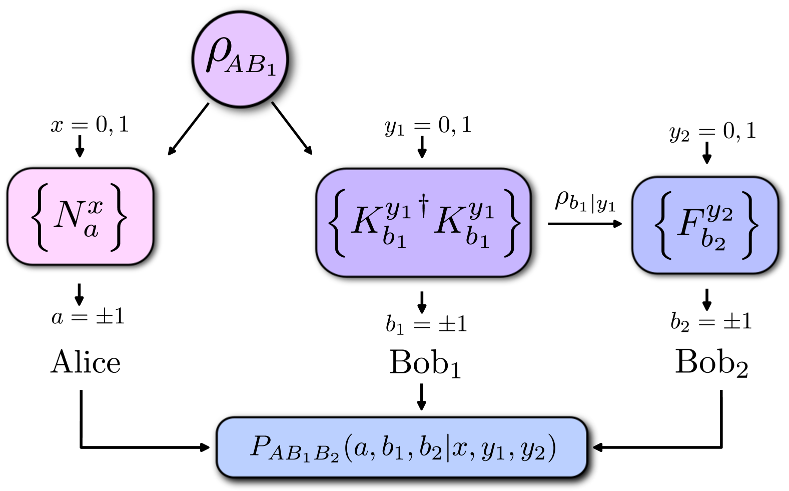
Figure 1: The sequential quantum scenario considered in this work.

The scheme proceeds as follows: a source prepares an unknown physical state $\rho_{AB_{1}}$, which is sent to both Alice and Bob₁. They locally randomly choose an input for their own device, which returns the outcome according to the result of a Positive Operator-Valued Measurement (POVM). After his operations, Bob₁ sends its post-measurement state to a second Bob, Bob₂, who also measures the state. We label Alice’s POVMs as $\{N^{x}_{a}\}$, Bob₁’s POVMs as $\{{K^{y_{1}}_{b_{1}}}^{\dagger}K^{y_{1}}_{b_{1}}\}$, for some appropriate set of Kraus operators, and Bob₂’s POVMs with $\{F^{y_{2}}_{b_{2}}\}$. We model the POVMs of Bob₁ with Kraus operators because we are interested in the post-measurement state left to Bob₂ which, given the input $y_{1}$, is

$$\rho_{AB_{2}}^{y_{1}}\equiv\sum_{b_{1}}K^{y_{1}}_{b_{1}}\rho_{AB_{1}}{K^{y_{1}}_{b_{1}}}^{\dagger}\,.$$ (1)

Throughout this process, all inputs are assumed to be independent, and there is no communication between Alice and the Bobs. However, Bob₁ is allowed to transmit information to Bob₂ after his measurement and, without loss of generality, this information is assumed to be passed through the action of the Kraus operators [16].

The conditional sequential correlations between the three users, $P_{AB_{1}B_{2}}(a,\mathbf{b}|x,\mathbf{y})$ with $\mathbf{b}=(b_{1},b_{2})$ and $\mathbf{y}=(y_{1},y_{2})$, are described through the Born rule:

$$P_{AB_{1}B_{2}}(a,\mathbf{b}|x,\mathbf{y})=\Tr\left[\rho_{AB_{1}}~N^{x}_{a}\otimes{K^{y_{1}}_{b_{1}}}^{\dagger}F^{y_{2}}_{b_{2}}K^{y_{1}}_{b_{1}}\right]\,.$$ (2)

From the above joint correlations, the marginals can be calculated by summing over the other parties’ outcomes. In particular, we can calculate the marginal correlations between Alice-Bob₁ and Alice-Bob₂ as

$$P_{AB_{1}}(a,b_{1}|x,y_{1}) =\Tr\left[\rho_{AB_{1}}~N^{x}_{a}\otimes{K^{y_{1}}_{b_{1}}}^{\dagger}K^{y_{1}}_{b_{1}}\right]\,,$$ (3)

$$P_{AB_{2}}(a,b_{2}|x,y_{1},y_{2}) =\Tr\left[\rho_{AB_{1}}~N^{x}_{a}\otimes\sum_{b_{1}}{K^{y_{1}}_{b_{1}}}^{\dagger}F^{y_{2}}_{b_{2}}K^{y_{1}}_{b_{1}}\right]\,.$$ (4)

From now on, we assume that such correlations are perfectly known and arise from independent and identically distributed (i.i.d.) runs of the protocol.

II.2 A class of sequential quantum protocols

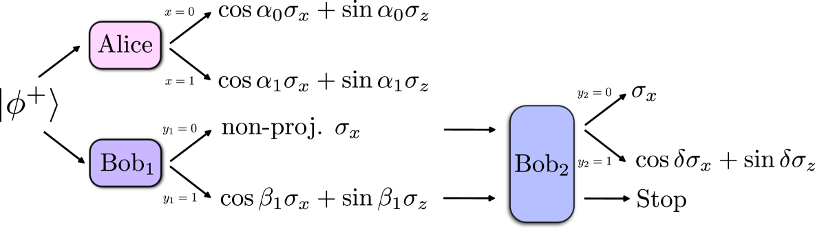
Figure 2: Scheme of measurement of the ideal sequential protocols.

Having outlined the sequential quantum scenario, we now present a class of sequential protocols for device-independent randomness generation. These protocols can be understood as sequential extensions of standard bipartite protocols that admit a self-testing certification from the correlations they produce. Therefore, we begin by considering a general self-testing qubit protocol with maximally entangled states, and then we present our systematic sequential construction.

When Alice and Bob share the two-qubit maximally entangled state

$$\ket{\phi^{+}}=\frac{\ket{00}+\ket{11}}{\sqrt{2}}\,,$$ (5)

the most general measurements that can be chosen to realize self-testing (in the two-inputs and two-outputs scenario) are described by the observables

$$\mathcal{A}_{0} =\cos\alpha_{0}\sigma_{x}+\sin\alpha_{0}\sigma_{z}\ ,$$ (6)

$$\mathcal{A}_{1} =\cos\alpha_{1}\sigma_{x}+\sin\alpha_{1}\sigma_{z}\ ,$$ (7)

$$\mathcal{B}_{0}^{\prime} =\sigma_{x}\ ,$$ (8)

$$\mathcal{B}_{1} =\cos\beta_{1}\sigma_{x}+\sin\beta_{1}\sigma_{z}\,,$$ (9)

with the parameters $\alpha_{0}$, $\alpha_{1}$, and $\beta_{1}$ chosen to satisfy the necessary and sufficient conditions discussed in [17]. We only consider real measurements: this stems from the fact that, once the necessary and sufficient conditions for the self-testing are met, we can always find local isometries mapping the measurements of Alice and Bob to combinations of $\sigma_{x}$ and $\sigma_{z}$ [17, 18]. In principle, we could have also defined $\mathcal{B}_{0}^{\prime}=\cos\beta_{0}\sigma_{x}+\sin\beta_{0}\sigma_{z}$. However, since the correlations $\expectationvalue{\mathcal{A}_{y}\mathcal{B}_{y}}=\cos(\alpha_{x}-\beta_{y})$, when evaluated on the state $\ket{\phi^{+}}$, depend only on the difference $\alpha_{x}-\beta_{y}$, we do not lose generality by assuming the angle $\beta_{0}=0$.

When extending the protocol in (5) and (6)-(9) sequentially, we aim to use the same state and modify one measurement into a non-projective one to prevent the loss of entanglement after it is performed. At the same time we want to preserve the self-testing properties to facilitate security proofs. To achieve this, we replace $\mathcal{B}_{0}^{\prime}$ by a POVM $\{{K^{0}_{b_{1}}}^{\dagger}K^{0}_{b_{1}}\}$ described by the Kraus operators

$$K^{0}_{+} \equiv\cos\theta\frac{\openone+\mathcal{B}_{0}^{\prime}}{2}+\sin\theta\frac{\openone-\mathcal{B}_{0}^{\prime}}{2}\,,$$ (10)

$$K^{0}_{-} \equiv\sin\theta\frac{\openone+\mathcal{B}_{0}^{\prime}}{2}+\cos\theta\frac{\openone-\mathcal{B}_{0}^{\prime}}{2}\,,$$ (11)

where we call $\theta\in\quantity[0,\frac{\pi}{4}]$ the strength parameter and $(\openone\pm\mathcal{B}_{0}^{\prime})/2$ define the two eigenspace projectors of $\mathcal{B}_{0}^{\prime}$. Note that for $\theta=0$ the two Kraus operators reduce to the two projectors of $\mathcal{B}_{0}^{\prime}$, while for $\theta=\frac{\pi}{4}$ they become proportional to the identity operator. After this measurement, the post-measurement state is sent to a second Bob, who performs a projective measurement equal to $\mathcal{B}_{0}^{\prime}$ for $y_{2}=0$ and a projective measurement in the form $\cos\delta\sigma_{x}+\sin\delta\sigma_{z}$, with $\delta\neq 0$, for $y_{2}=1$.

The key point is that, for the choice $y_{1}=0$ and $y_{2}=0$, Bob₂ measures $\mathcal{B}_{0}^{\prime}$ after Bob₁ has performed a non-projective version of $\mathcal{B}_{0}^{\prime}$ itself. This implies that the correlations $P_{AB_{2}}(a,b_{2}|x,0,0)$ between Alice and Bob₂ are equivalent to those that would be obtained with a projective measurement of $\mathcal{B}_{0}^{\prime}$, i.e., those which allow the self-testing. To check this property, we evaluate (4) for $y_{1}=0$ and $y_{2}=0$:

$$\begin{split}P_{AB_{2}}&(a,b_{2}|x,0,0)=\sum_{b_{1}}P_{AB_{1}B_{2}}(a,b_{1},b_{2}|x,0,0)\\ &=\sum_{b_{1}}\Tr\left[\rho_{AB_{1}}~N^{x}_{a}\otimes{K^{0}_{b_{1}}}^{\dagger}\frac{\openone+b_{2}\mathcal{B}_{0}^{\prime}}{2}K^{0}_{b_{1}}\right]\\ &=\Tr\left[\rho_{AB_{1}}~N^{x}_{a}\otimes\frac{\openone+b_{2}\mathcal{B}_{0}^{\prime}}{2}\right]\,.\end{split}$$ (12)

Last equality holds because the projectors of $\mathcal{B}_{0}^{\prime}$ are invariant under the action of the Kraus operators $K^{0}_{b_{1}}$:

$$\sum_{b_{1}}K^{0}_{b_{1}}\frac{\openone+b_{2}\mathcal{B}_{0}^{\prime}}{2}K^{0}_{b_{1}}=\frac{\openone+b_{2}\mathcal{B}_{0}^{\prime}}{2}\,.$$ (13)

Thanks to this property, after the sequential extension, we can still rely on the self-testing properties of the correlations, which we will leverage to prove randomness in a device-independent scenario.

The ideal sequential protocol, depicted in Fig. 2, can be summarized as follows. First, Alice and Bob₁ share a maximally entangled state, $\ket{\phi^{+}}_{AB_{1}}$. Alice randomly selects one of two inputs, $x\in\{0,1\}$, corresponding to the two observables $\mathcal{A}_{x}$ defined in (6) and (7). Bob₁ also randomly chooses between two inputs, $y_{1}\in\{0,1\}$. Input $y_{1}=1$ corresponds to a projective measurement of $\mathcal{B}_{1}$, while $y_{1}=0$ corresponds to a non-projective measurement of $\mathcal{B}_{0}^{\prime}$, implemented through the two Kraus operators (10) and (11). If $y_{1}=0$, Bob₁ sends its post-measurement state to Bob₂. Bob₂ then randomly selects one of two inputs, $y_{2}\in\{0,1\}$, corresponding to either a projective measurement of $\mathcal{B}_{0}^{\prime}$ or a measurement of the observable $\cos\delta\,\sigma_{x}+\sin\delta\,\sigma_{z}$. Otherwise, if Bob₁ chooses $y_{1}=1$, then Bob₂ does nothing, ending the protocol.

II.3 Device-independent framework for sequential quantum correlations

We now recall the projective framework introduced in [15] for describing sequential quantum correlations in a device-independent scenario. We adopt this framework for our analytical proofs.

In a device-independent sequential scenario, the experimental correlations (2) are assumed to derive from an unknown tripartite state $\ket{\psi}\in\mathcal{H}_{A}\otimes\mathcal{H}_{B}\otimes\mathcal{H}_{E}$ measured by Alice’s and Bob’s unknown projectors acting on the Hilbert spaces $\mathcal{H}_{A}$ and $\mathcal{H}_{B}$ respectively. $\mathcal{H}_{E}$ is an arbitrary Hilbert space where a potential eavesdropper Eve acts. Therefore, the sequential correlations can be calculated as

$$P_{AB_{1}B_{2}}(a,\mathbf{b}|x,\mathbf{y})=\expectationvalue{\Lambda^{x}_{a}\otimes\Pi^{y_{1}}_{b_{1}}\Pi^{y_{1}y_{2}}_{b_{2}}\otimes\openone_{E}}{\psi}\,.$$ (14)

In this framework, Alice’s POVMs are replaced by the projective measurements $\{\Lambda^{x}_{a}\}$, and the pair of Bobs, represented by the four-outcomes POVMs $\{{K^{y_{1}}_{b_{1}}}^{\dagger}F^{y_{2}}_{b_{2}}K^{y_{1}}_{b_{1}}\}$ in (2), is replaced by just one Bob with the product of the projectors $\Pi^{y_{1}}_{b_{1}}$ and $\Pi^{y_{1}y_{2}}_{b_{2}}$. These projectors satisfy specific mathematical constraints deriving from the sequentiality, namely they satisfy the commutation relation $\left[\Pi^{y_{1}}_{b_{1}},\Pi^{y_{1}y_{2}}_{b_{2}}\right]=0$ for any input pair $y_{1},y_{2}$ [15]. These operators can be used to evaluate the marginal distributions of Bob₁ and Bob₂, respectively:

$$P_{AB_{1}}(a,b_{1}|x,y_{1}) =\expectationvalue{\Lambda^{x}_{a}\otimes\Pi^{y_{1}}_{b_{1}}\otimes\openone_{E}}{\psi}\,,$$ (15)

$$P_{AB_{2}}(a,b_{2}|x,y_{1},y_{2}) =\expectationvalue{\Lambda^{x}_{a}\otimes\Pi^{y_{1}y_{2}}_{b_{2}}\otimes\openone_{E}}{\psi}\,.$$ (16)

The fact that $\Pi^{y_{1}}_{b_{1}}$ and $\Pi^{y_{1}y_{2}}_{b_{1}}$ commute guarantees that the product $\Pi^{y_{1}}_{b_{1}}\Pi^{y_{1}y_{2}}_{b_{1}}$ is a well-defined measurable projector. In addition, since every measurement of the protocol has two possible outcomes, we can construct Hermitian and unitary operators from the projectors in (14) as:

$$A_{x} \equiv\Lambda^{x}_{+}-\Lambda^{x}_{-}\ ,$$ (17)

$$B_{y_{1}} \equiv\Pi^{y_{1}}_{+}-\Pi^{y_{1}}_{-}\ ,$$ (18)

$$B_{y_{1}y_{2}} \equiv\Pi^{y_{1}y_{2}}_{+}-\Pi^{y_{1}y_{2}}_{-}\ ,$$ (19)

$$\quantity[B_{y_{1}},B_{y_{1}y_{2}}] =0\,.$$ (20)

Using these operators we can provide an alternative equivalent parametrization for the sequential correlations (14). In particular, the observables $B_{1}$ and $B_{00}$ generate the same correlations as $\mathcal{B}_{1}$ and $\mathcal{B}_{0}^{\prime}$, and hence they can be self-tested.

III Results

III.1 Security and extremality of correlations

In this section, we explain why the correlations produced by the sequential construction of Sec. II.2 can be used for device-independent security. By security, we mean that for any possible quantum realization of the sequential correlations, the following holds:

$$\expectationvalue{\Lambda^{x}_{a}\otimes\Pi^{y_{1}}_{b_{1}}\Pi^{y_{1}y_{2}}_{b_{2}}\otimes E}{\psi}=P_{AB_{1}B_{2}}(a,\mathbf{b}|x,\mathbf{y})\expectationvalue{E}\,,$$ (21)

where $E$ is an arbitrary Hermitian quantum operator measured by Eve. As shown in [19], this condition is equivalent to requiring that the correlations are extremal, meaning they cannot be expressed as a combination of other quantum correlations. Intuitively, this implies that an eavesdropper cannot decompose them to gain an advantage. See also Appendix A for more details.

A necessary condition for the correlations to be extremal (and hence secure) is that they lie on the boundary of the set of all realizable quantum correlations [7]. In our scenario, we denote this set as $\mathcal{Q}_{SEQ}$, which includes all quantum correlations between one Alice and two Bobs that are compatible with the sequentiality constraints [16]. The fact that some correlations lie on the boundary of $\mathcal{Q}_{SEQ}$ can be certified by demonstrating that they saturate a Tsirelson bound [20, 5, 16]. Indeed, relying on the results of [21], we can explicitly construct a Tsirelson bound that is saturated by the correlations produced by the sequential protocol of Sec. II.2, as we now show.

First, recall that we constructed our class of sequential protocol starting from a non-sequential class, (5) and (6)–(9), whose correlations self-test state and measurements [17]. Then, thanks to the invariance (13), also the correlations Alice-Bob₁, $P_{AB_{1}}(a,b_{1}|x,1)$, and the correlations Alice-Bob₂, $P_{AB_{2}}(a,b_{2}|x,0,0)$ certify, up to local isometries, that the measurements $A_{0}$, $A_{1}$, $B_{00}$ and $B_{1}$ are the ones in (6)–(9), and the part of the state on which they act is $\ket{\phi^{+}}$.

Regarding the correlations of the remaining operators, $B_{0}$ and $B_{01}$, we observe that they are realized by a rank-one four-outcomes POVM with elements $\{{K^{0}_{b_{1}}}^{\dagger}F^{1}_{b_{2}}K^{0}_{b_{1}}\}$. Then, using the results of [21], the Tsirelson bound we consider is written as

$$\expectationvalue{S_{\theta,\delta}}=0\,,$$ (22)

where the Bell operator $S_{\theta,\delta}$ has the form

$$S_{\theta,\delta}\equiv\frac{1}{2}\Bigl{[}\openone-X_{A}\Bigl{(}c_{1}B_{01}+c_{2}B_{0}\Bigr{)}-Z_{A}\Bigl{(}c_{3}B_{01}+c_{4}B_{0}\Bigr{)}\Bigr{]}\,.$$ (23)

The operators $X_{A}$ and $Z_{A}$ are defined from $A_{0}$ and $A_{1}$ such that in the ideal protocol they coincide with $\sigma_{x}$ and $\sigma_{z}$ respectively:

$$\begin{split}X_{A}&\equiv\frac{\sin\alpha_{1}A_{0}+\sin\alpha_{0}A_{1}}{\sin(\alpha_{1}-\alpha_{0})}\ ,\\ Z_{A}&\equiv\frac{\cos\alpha_{1}A_{0}+\cos\alpha_{0}A_{1}}{\sin(\alpha_{0}-\alpha_{1})}\,,\end{split}$$ (24)

while the coefficients $c_{i}$ depend on the strength parameter $\theta$ and on the angle $\delta$ (see Eq. (54) in Appendix B). Since it holds that $\expectationvalue{S_{\theta,\delta}}=\expectationvalue*{S_{\theta,\delta}^{\dagger}S_{\theta,\delta}}\geq 0$, then Eq. (22) implies

$$S_{\theta,\delta}\ket{\psi}=0\,,$$ (25)

from which the security condition can be verified. All the calculations are provided in Appendix B.3.

The proof holds for any value of the strength parameter $\theta$, except for the extremal values $0$ and $\frac{\pi}{4}$. This can be explained by considering that when $\theta=0$, Bob₁ is performing a projective measurement and hence Bob₂ receives a state that is no longer entangled. In contrast, when $\theta=\frac{\pi}{4}$, although Bob₁ shares a maximally entangled state, his outcomes are completely uncorrelated with both Alice and Bob₂, because his measurement operators are proportional to the identity. However, as shown by the following examples, setting $\theta\in\quantity{0,\frac{\pi}{4}}$ does not necessarily imply that the randomness drops to zero, but rather to a value that depends on the specific sequential protocol chosen.

The security condition (21) guarantees that the quantum min-entropy reduces to the classical min-entropy, and the worst-case conditional von Neumann entropy reduces to the Shannon entropy, as we show in Appendix A. These quantities are defined in the following way [22]. Suppose that we aim to generate random numbers from the outcomes obtained by the inputs $x^{\star}$ and $\mathbf{y}^{\star}$. By using the projective framework of (14), we define the classical-quantum post-measurement state associated to the measurements $x^{\star}$ and $\mathbf{y}^{\star}$ (not to be confused with the post-measurement state of Bob₁ introduced in Section II.1):

$$\rho_{ABE}^{post}\equiv\sum_{a,\mathbf{b}}P_{AB_{1}B_{2}}(a,\mathbf{b}|x^{\star},\mathbf{y}^{\star})\outerproduct{a,\mathbf{b}}{a,\mathbf{b}}\otimes\tau_{E}^{a,\mathbf{b}}\,.$$ (26)

In the above definition, $\outerproduct{a,\mathbf{b}}{a,\mathbf{b}}\in\mathcal{H}_{A^{\prime}}\otimes\mathcal{H}_{B^{\prime}}$ is a classical state in which Alice and Bob register their measurement results, and $\tau_{E}^{a,\mathbf{b}}\in\mathcal{H}_{E}$ is the reduced state of Eve:

$$\tau_{E}^{a,\mathbf{b}}\equiv\frac{\Tr_{AB}\quantity[\Lambda^{x^{\star}}_{a}\otimes\Pi^{y_{1}^{\star}}_{b_{1}}\Pi^{y_{1}^{\star},y_{2}^{\star}}_{b_{2}}\otimes\openone_{E}~\outerproduct{\psi}{\psi}]}{P_{AB_{1}B_{2}}(a,\mathbf{b}|x^{\star},\mathbf{y}^{\star})}\,.$$ (27)

The worst-case conditional von Neumann entropy is defined as

$$H(AB|E)\equiv\min_{\rho_{ABE}^{post}}\left[H(AB)_{\rho_{ABE}^{post}}-H(E)_{\rho_{ABE}^{post}}\right]\ ,$$ (28)

where the minimization is over all the possible classical-quantum post-measurements states compatible with the observed probability distribution. The min-entropy is defined as $H_{min}\equiv-\log_{2}G(AB|E)$, where $G(AB|E)$ is the guessing probability

$$G(AB|E)\equiv\!\!\!\max_{E_{a\mathbf{b}},\tau_{E}^{a,\mathbf{b}}}\sum_{a,\mathbf{b}}\!P_{AB_{1}B_{2}}(a,\mathbf{b}|x^{\star},\mathbf{y}^{\star})\Tr_{E}\quantity[E_{a\mathbf{b}}\tau_{E}^{a,\mathbf{b}}]$$ (29)

where, again, the maximization must be compatible with the experimental data and $E_{a\mathbf{b}}$ is a generic projector of Eve. It turns out that, if the security definition (21) holds, then the post-measurement state (26) has a product form $\rho_{ABE}^{post}=\rho_{AB}^{post}\otimes\rho_{E}^{post}$. Therefore, $H(AB|E)$ reduces to the Shannon entropy of $P_{AB_{1}B_{2}}(a,\mathbf{b}|x^{\star},\mathbf{y}^{\star})$, and the guessing probability to the best classical guess $\max_{a,\mathbf{b}}P_{AB_{1}B_{2}}(a,\mathbf{b}|x^{\star},\mathbf{y}^{\star})$.

In our protocol the input sequence $\mathbf{y}=(0,0)$ is used to generate the self-testing correlations, while the sequence $\mathbf{y}^{\star}=(0,1)$ is chosen for randomness generation. To maximize the entropy, $\delta$ must be chosen based on the values of $\alpha_{0}$ (if $x^{\star}=0$) or $\alpha_{1}$ (if $x^{\star}=1$). The complete parametric expressions for the min-entropy and von Neumann entropy are provided in Eq. (81) in Appendix B.3.

III.2 Example 1: Sequential CHSH

In [15], the authors proposed a sequential extension of the CHSH protocol and analytically proved the local min-entropy of a specific Bobs’ input sequence in case of ideal correlations. With respect to the general class of protocols presented before, the sequential CHSH is defined by setting $\alpha_{0}=\frac{\pi}{4}$, $\alpha_{1}=\frac{3\pi}{4}$, $\beta_{1}=\frac{\pi}{2}$ and $\delta=\frac{\pi}{2}$, and by performing an Hadamard transformation on Bobs’ measurements. We can conclude that whatever input (global or local) is chosen for randomness generation, under ideal conditions, the min-entropy coincides with the entropy of the most probable outcome, and the von Neumann entropy with the Shannon entropy of the outcomes probability distribution. See Fig. 3 for a plots of the two entropies when the randomness is generated by the measurements identified by $x^{\star}=0$, $y_{1}^{\star}=0$ and $y_{2}^{\star}=1$. For $\theta\in\quantity{0,\frac{\pi}{4}}$ the min-entropy reduces to $\approx 1.2$ bits, while the von Neumann entropy reduces to $\approx 1.6$ bits.

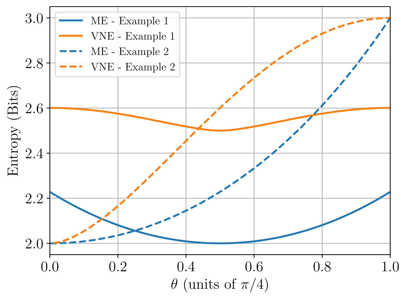
Figure 3: Min-entropy (ME) and von Neumann entropy (VNE) of the protocols described in Example 1 (continuous line) and Example 2 (dashed line).

III.3 Example 2: Sequential extension of [23]

The previous example is not optimal for global randomness generation because the ideal measurements of Alice and the Bobs are strongly correlated. Therefore, we could look for a protocol in which Alice has at least one measurement that is loosely correlated with the Bobs’ measurements. One feasible candidate is the sequential extension of the protocol proposed in [23], saturating the Bell expression

$$\expectationvalue{I_{\omega}}=\expectationvalue{A_{0}B_{0}}+\frac{\expectationvalue{A_{0}B_{1}}+\expectationvalue{A_{1}B_{0}}}{\sin\omega}-\frac{\expectationvalue{A_{1}B_{1}}}{\cos 2\omega}\,,$$ (30)

for $\omega\in(0,\frac{\pi}{6}]$. The Tsirelson bound is given by $2\cos^{3}\omega/(\cos 2\omega\sin\omega)$, and the optimal non-sequential strategy is to set $\alpha_{0}=\frac{\pi}{2}$, $\alpha_{1}=-\omega$ and $\beta_{1}=\omega+\frac{\pi}{2}$. For the sequential extension, we set $\delta=\frac{\pi}{2}$, since, as can be verified, it maximizes the generation of randomness.

For a plot of the min- and von Neumann entropy generated by the measurements identified by $x^{\star}=0$, $y_{1}^{\star}=0$ and $y_{2}^{\star}=1$ with $\omega=\frac{\pi}{6}$, see Fig. 3. It shows that both entropies are always greater than $2$ bits for $\theta\in(0,\frac{\pi}{4})$ and reduce to $2$ bits only for $\theta\in\quantity{0,\frac{\pi}{4}}$.

IV Conclusions

We have proposed a class of simple quantum sequential protocols, relying on measurements of Pauli observables on a maximally entangled qubit state and designed for device-independent cryptographic tasks.

Under device-independent and i.i.d. assumptions, we have analytically demonstrated that the ideal sequential correlations arising in this scenario can serve cryptographic purposes, as these correlations are shown to be extremal within the set of sequential quantum correlations, and extremality ensures that the optimal strategy for any potential eavesdropper attempting to guess the random bits is limited to betting on the most probable measurement outcomes. We leave the study of the robustness against noise and detection efficiency as future work, which can already be pursued by leveraging numerical methods [24, 25, 26, 27, 28]. Moreover, although we considered a scenario with three parties choosing between two possible dichotomic measurements, more complex scenarios can be explored. For example, the number of sequential parties could be increased, or the number of inputs could be expanded by considering self-testing protocols that involve all Pauli matrices [29] and by extending them sequentially. In that case, the three users could achieve 3 bits of global randomness, independently of the strength parameter of Bob₁. Additionally, we note that the maximally entangled state is not necessary for applying our sequential construction. One may further generalize our results by considering non-maximally entangled states, exploiting the self-testing properties of some tilted Bell inequality [30].

We emphasize that the device-independent security of our sequential protocols explicitly relies on the sequential ordering between the two Bobs. Consequently, a proper device-independent implementation must not only address known loopholes [31, 32] but also ensure that Bob₁ receives his measurement outcomes before Bob₂ does. This requirement excludes pure photonic implementations with a tree-like sequential measurement structure, such as the ones in [11, 14, 15], where the whole outcomes history is retrieved with a photon detector placed at Bob₂’s location. Although pure photonic implementations could leverage quantum non-demolition measurements of photon states, they remain inefficient [33, 34]. Nevertheless, while photons may not be the ideal candidates for these protocols at present, alternative implementations based on matter-based quantum states and measurements could be explored [35, 36, 37, 38, 39, 40].

The key feature of the proposed sequential scheme is the inclusion of a non-projective measurement, which can be viewed as a weak version of an observable, and the subsequent measurement of the same observable. It is well-established that quantum non-projective measurements exhibit a trade-off between information gain and state disturbance [10]: stronger measurements provide more information but induce greater disturbance on the measured state. Accordingly with [15], our results show that even when the measurement strength approaches zero, yielding arbitrarily small information gain, the measurement outcomes still remain random in a device-independent setting. The results of this work can open avenues for future research on device-independent randomness generation and key distribution protocols. For example, we note a connection between the sequential scenario considered in this work and the routed Bell experiments [41, 42, 43], in which sequentiality is present between the switch station and the two possible subsequent Bobs. Could the methods adopted here further improve the performance of protocols based on routed Bell experiments? In addition to their application in device-independent security protocols, sequential quantum schemes are also valuable for investigating fundamental aspects of quantum mechanics, such as contextuality [44, 45, 46, 47, 48]. Our findings may be useful for advancing research in this area as well. For example, they could help in finding new inequalities whose violation certifies contextuality in the same way that Bell inequalities certify nonlocality.

APPENDIX A Extremality and security of the sequential quantum correlations

In this appendix we recall the device-independent sequential scenario, the definition of extremal correlations, and the connection between extremality and the security condition defined in the main text. Finally, we show that when security condition holds, the correlations certify the maximal randomness obtainable from the observed outcomes.

A.1 Relation between extremality and security

We utilize the projective framework reviewed in the main text and presented in [16, 15]. In particular, we consider a pure quantum state $\ket{\psi}\in\mathcal{H}_{A}\otimes\mathcal{H}_{B}\otimes\mathcal{H}_{E}$ and some sets of measurements, $\quantity{\Lambda^{x}_{a}}$ and $\quantity{\Pi^{y_{1}}_{b_{1}},\Pi^{y_{1},y_{2}}_{b_{2}}}$, acting on $\mathcal{H}_{A}$ and $\mathcal{H}_{B}$ respectively. We will refer to the set $\quantity{\ket{\psi},\quantity{\Lambda^{x}_{a}},\quantity{\Pi^{y_{1}}_{b_{1}},\Pi^{y_{1},y_{2}}_{b_{2}}}}$ as a quantum realization of the correlations. The Alice-Bob₁-Bob₂ correlations are retrieved through the Born rule by tracing out over Eve’s space $\mathcal{H}_{E}$:

$$P_{AB_{1}B_{2}}(a,\mathbf{b}|x,\mathbf{y})=\expectationvalue{\Lambda^{x}_{a}\otimes\Pi^{y_{1}}_{b_{1}}\Pi^{y_{1},y_{2}}_{b_{2}}\otimes\openone_{E}}{\psi}=\Tr_{AB}\quantity[\Lambda^{x}_{a}\otimes\Pi^{y_{1}}_{b_{1}}\Pi^{y_{1},y_{2}}_{b_{2}}~\rho_{AB}]\,,$$ (31)

where we defined $\rho_{AB}\equiv\Tr_{E}[\outerproduct{\psi}{\psi}]$. The operators in the above expression satisfy the orthogonality and normalization constraints:

$$\begin{split}\Lambda^{x}_{a}\Lambda^{x}_{a^{\prime}}&=\delta_{aa^{\prime}}\Lambda^{x}_{a}\ ,\\ \Pi^{y_{1}}_{b_{1}}\Pi^{y_{1}}_{b_{1}^{\prime}}&=\delta_{b_{1}b_{1}^{\prime}}\Pi^{y_{1}}_{b_{1}}\ ,\\ \Pi^{y_{1}y_{2}}_{b_{2}}\Pi^{y_{1}y_{2}}_{b_{2}^{\prime}}&=\delta_{b_{2}b_{2}^{\prime}}\Pi^{y_{1}y_{2}}_{b_{2}}\ ,\\ \sum_{a}\Lambda^{x}_{a}&=\openone_{A}\ ,\\ \sum_{b_{1}}\Pi^{y_{1}}_{b_{1}}&=\sum_{b_{2}}\Pi^{y_{1}y_{2}}_{b_{2}}=\openone_{B}\,.\end{split}$$ (32)

Moreover, from the sequential constraints, the following commutation holds

$$\left[\Pi^{y_{1}}_{b_{1}},\Pi^{y_{1}y_{2}}_{b_{2}}\right]=0\,.$$ (33)

The operations that Eve can perform in her own space can be assumed without loss of generality to be some set of projectors $\quantity{E_{e}}$ satisfying $\sum_{e}E_{e}=\openone_{E}$. Therefore, the correlations (31) can be written as a convex sum of some set of (possibly different) correlations parameterized by the index $e$:

$$\begin{split}P_{AB_{1}B_{2}}(a,\mathbf{b}|x,\mathbf{y})&=\sum_{e}\Tr_{AB}\quantity[\Lambda^{x}_{a}\otimes\Pi^{y_{1}}_{b_{1}}\Pi^{y_{1},y_{2}}_{b_{2}}~\Tr_{E}\quantity[E_{e}\outerproduct{\psi}{\psi}]]\\ &=\sum_{e}P_{E}(e)\Tr_{AB}\quantity[\Lambda^{x}_{a}\otimes\Pi^{y_{1}}_{b_{1}}\Pi^{y_{1},y_{2}}_{b_{2}}~\rho_{AB}^{e}]\\ &=\sum_{e}P_{E}(e)P_{AB_{1}B_{2}}(a,\mathbf{b}|x,\mathbf{y},e)\,,\end{split}$$ (34)

where we defined the normalized states $\rho_{AB}^{e}\equiv\Tr_{E}[E_{e}\outerproduct{\psi}{\psi}]/P_{E}(e)$ and $P_{E}(e)\equiv\Tr_{E}[E_{e}\Tr_{AB}[\outerproduct{\psi}{\psi}]]$. We say that the correlations $P_{AB_{1}B_{2}}(a,\mathbf{b}|x,\mathbf{y})$ are extremal if they cannot be written as a convex combination of other different correlations. In other terms, if $P_{AB_{1}B_{2}}(a,\mathbf{b}|x,\mathbf{y})$ are extremal and (34) holds, then it must be $P_{AB_{1}B_{2}}(a,\mathbf{b}|x,\mathbf{y},e)=P_{AB_{1}B_{2}}(a,\mathbf{b}|x,\mathbf{y})$ for each $e$. Since the aim of Eve is to guess the outcomes of the three users by leveraging the knowledge of the final convex decomposition in (34), extremality guarantees that Eve cannot have more information about the experimental correlations than the information that Alice, Bob₁ and Bob₂ have.

As shown in [19], the extremality of correlations is in one to one correspondence with the security of correlations. For the sake of clarity, we adapt the discussion of [19] to our sequential scenario. A probability distribution $P_{AB_{1}B_{2}}(a,\mathbf{b}|x,\mathbf{y})$ is called secure if it does not factorize, $P_{AB_{1}B_{2}}\neq P_{A}(a|x)P_{B_{1}B_{2}}(\mathbf{b}|\mathbf{y})$, and if for any quantum realization and any operator $E$ it holds

$$\expectationvalue{\Lambda^{x}_{a}\otimes\Pi^{y_{1}}_{b_{1}}\Pi^{y_{1},y_{2}}_{b_{2}}\otimes E}{\psi}=\Tr[E\outerproduct{\psi}{\psi}]P_{AB_{1}B_{2}}(a,\mathbf{b}|x,\mathbf{y})\,.$$ (35)

With this definition, it is possible to show that a probability distribution $P_{AB_{1}B_{2}}(a,\mathbf{b}|x,\mathbf{y})$ is secure if and only if it is extremal in $\mathcal{Q}_{SEQ}\setminus\mathcal{C}$, with $\mathcal{C}$ the set of correlations that can be written as convex combination of results of local deterministic measurements [19]. Note that, since signaling is present from Bob₁ to Bob₂, we consider them as a unique Bob with four inputs and four outputs, whose measurements are defined in terms of the projectors ${\mathsf{B}}^{y_{1}y_{2}}_{b_{1}b_{2}}\equiv\Pi^{y_{1}}_{b_{1}}\Pi^{y_{1}y_{2}}_{b_{2}}$ satisfying sequentiality constraints. See also [16] for further details.

We highlight that, in [19], the authors imposed only commutation between operators of separated parties, rather than the tensor product structure of the entire Hilbert space. This is not an issue for our proofs, since we can always redefine the local operators to act on the entire Hilbert space as $\Lambda^{x}_{a}\equiv\Lambda^{x}_{a}\otimes\openone_{B}\otimes\openone_{E}$, and similarly for Bob’s and Eve’s operators, thereby realizing a strategy with commuting operators. In fact, although we specifically consider tensor product realizations, the following demonstrations can be expressed solely by invoking the commutation between Alice, Bob, and Eve. Therefore, they also apply to the more general case of commuting realizations.

A.2 Randomness from security

We now show that security guarantees that maximal randomness can be generated from the correlations. From this point forward, we denote the set of chosen inputs used to generate randomness as $\mathbf{r}\equiv(x^{\star},y_{1}^{\star},y_{2}^{\star})$. In particular, we show that the worst-case quantum conditional min-entropy, $H_{min}(AB|E)$ reduces to $-\log_{2}\max_{ab_{1}b_{2}}P_{AB_{1}B_{2}}(a,\mathbf{b}|\mathbf{r})$, while the worst-case conditional von Neumann entropy, $H(AB|E)$, reduces to the Shannon entropy $-\sum_{ab_{1}b_{2}}P_{AB_{1}B_{2}}(a,\mathbf{b}|\mathbf{r})\log_{2}\quantity[P_{AB_{1}B_{2}}(a,\mathbf{b}|\mathbf{r})]$. These two quantities are calculated on the classical-quantum post-measurement state defined as

$$\rho_{ABE}^{post}\equiv\sum_{a,\mathbf{b}}P_{AB_{1}B_{2}}(a,\mathbf{b}|\mathbf{r})\outerproduct{a,\mathbf{b}}{a,\mathbf{b}}\otimes\tau_{E}^{a,\mathbf{b}}\quad\in\mathcal{H}_{A^{\prime}}\otimes\mathcal{H}_{B^{\prime}}\otimes\mathcal{H}_{E}\,,$$ (36)

where $\mathcal{H}_{A^{\prime}}$ and $\mathcal{H}_{B^{\prime}}$ are two Hilbert spaces in which Alice and Bob register their outcomes, $\outerproduct{a,\mathbf{b}}{a,\mathbf{b}}=\outerproduct{a}{a}\otimes\outerproduct{\mathbf{b}}{\mathbf{b}}$, $\sum_{a}\outerproduct{a}{a}=\openone_{A^{\prime}}$, $\sum_{\mathbf{b}}\outerproduct{\mathbf{b}}{\mathbf{b}}=\openone_{B^{\prime}}$ and

$$\tau_{E}^{a,\mathbf{b}}\equiv\frac{\Tr_{AB}\quantity[\Lambda^{x^{\star}}_{a}\otimes\Pi^{y_{1}^{\star}}_{b_{1}}\Pi^{y_{1}^{\star},y_{2}^{\star}}_{b_{2}}\otimes\openone_{E}~\outerproduct{\psi}{\psi}]}{P_{AB_{1}B_{2}}(a,\mathbf{b}|\mathbf{r})}\quad\in\mathcal{H}_{E}\,.$$ (37)

The statement regarding the two entropies is proved by showing that security implies that the post-measurement state is in product form with Eve’s space. Eve’s outcomes are distributed according

$$P_{E}(e|a,\mathbf{b})=\Tr_{E}[E_{e}~\tau_{E}^{a,\mathbf{b}}]=\frac{P_{AB_{1}B_{2}}(a,\mathbf{b},e|\mathbf{r})}{P_{AB_{1}B_{2}}(a,\mathbf{b}|\mathbf{r})}=\frac{\expectationvalue{\Lambda^{x}_{a}\otimes\Pi^{y_{1}}_{b_{1}}\Pi^{y_{1},y_{2}}_{b_{2}}\otimes E_{e}}{\psi}}{P_{AB_{1}B_{2}}(a,\mathbf{b}|\mathbf{r})}\,,$$ (38)

and imposing (35) we obtain $P_{E}(e|a,\mathbf{b})=P_{E}(e)$, indicating that Eve’s outcomes do not depend on the ones of Alice and the Bobs. Since we are not fixing a particular quantum realization, and (35) holds for any Eve’s measurement, the states $\tau_{E}^{a,\mathbf{b}}$ and $\Tr_{AB}[\outerproduct{\psi}{\psi}]$ are equal. Therefore, the post-measurement state reduces to

$$\rho_{ABE}^{post}=\quantity[\sum_{a,\mathbf{b}}P_{AB_{1}B_{2}}(a,\mathbf{b}|\mathbf{r})\outerproduct{a,\mathbf{b}}{a,\mathbf{b}}]\otimes\Tr_{AB}[\outerproduct{\psi}{\psi}]\equiv\rho^{post}_{AB}\otimes\rho^{post}_{E}\,.$$ (39)

We can then directly conclude about the conditional von Neumann entropy. Indeed, by definition $H(AB|E)_{\rho}=H(\rho^{post}_{ABE})-H(\rho^{post}_{E})$ and, since the $\rho^{post}_{ABE}$ has a product form, for additivity we obtain that $H(AB|E)_{\rho}=H(\rho^{post}_{AB})$. Finally, since $\rho^{post}_{AB}$ has a diagonal form, its von Neumann entropy is the Shannon entropy of $P_{AB_{1}B_{2}}(a,\mathbf{b}|\mathbf{r})$.

For the min-entropy we calculate the guessing probability as [49, 50, 51]

$$\begin{split}G(AB|E)&\equiv\max_{\quantity{E_{a\mathbf{b}}}}\sum_{a,\mathbf{b}}P_{AB_{1}B_{2}}(a,\mathbf{b}|\mathbf{r})\Tr_{E}[E_{a\mathbf{b}}\tau_{E}^{a,\mathbf{b}}]\\ &=\sum_{a,\mathbf{b}}P_{AB_{1}B_{2}}(a,\mathbf{b}|\mathbf{r})\max_{\quantity{E_{a\mathbf{b}}}}\Tr_{E}[E_{a\mathbf{b}}\rho^{post}_{E}]\\ &=\sum_{a,\mathbf{b}}P_{AB_{1}B_{2}}(a,\mathbf{b}|\mathbf{r})P_{E}(a,\mathbf{b})\leq\max_{a,\mathbf{b}}P_{AB_{1}B_{2}}(a,\mathbf{b}|\mathbf{r})\,.\end{split}$$ (40)

Finally, $H_{min}(AB|E)=-\log_{2}G(AB|E)=-\log_{2}\max_{a,\mathbf{b}}P_{AB_{1}B_{2}}(a,\mathbf{b}|\mathbf{r})$.

APPENDIX B Proof of security of the sequential correlations

In this appendix, we propose a specific quantum realization of the sequential correlations using projective measurements. Such realization is obtained from the one in Sec. II.2 through a Stinespring dilation of the POVMs. Furthermore, we recall in detail the expression of the Tsirelson bound and, using its maximal saturation, we prove the security of the correlations.

B.1 Sequential correlations with projective measurements

As introduced in the main text, sequential quantum correlations can always be written in terms of a pure state and projective measurements. Here we show such state and measurements for the sequential protocols proposed in the main text.

The state is

$$\ket{\psi}=\ket{\phi^{+}}_{AB}\Bigl{[}\cos\theta\ket{+}_{B^{\prime}}+\sin\theta\ket{-}_{B^{\prime}}\Bigr{]}\quad\in\mathcal{H}_{A}\otimes\mathcal{H}_{B}\otimes\mathcal{H}_{B^{\prime}}=\mathbb{C}^{2}\otimes\mathbb{C}^{2}\otimes\mathbb{C}^{2}\,,$$ (41)

where the kets $\quantity{\ket{\pm}}$ are the eigenstates of $\sigma_{x}$.

Alice’s measurements remain the same introduced in the main text:

$$A_{0} =\cos\alpha_{0}\sigma_{x}+\sin\alpha_{0}\sigma_{z}\,,$$ (42)

$$A_{1} =\cos\alpha_{1}\sigma_{x}+\sin\alpha_{1}\sigma_{z}\,,$$ (43)

and act on $\mathcal{H}_{A}$. On Bob’s side, the measured observables are

$$B_{0} =\sigma_{x}\otimes\sigma_{x}\ ,$$ (44)

$$B_{1} =\Bigl{[}\cos\beta_{1}\sigma_{x}+\sin\beta_{1}\sigma_{z}\Bigr{]}\otimes\openone_{B^{\prime}}\ ,$$ (45)

$$B_{00} =\sigma_{x}\otimes\openone_{B^{\prime}}\ ,$$ (46)

$$B_{01} =\cos\delta\sigma_{x}\otimes\openone_{B^{\prime}}+\sin\delta\sigma_{z}\otimes\sigma_{z}\,$$ (47)

and act on $\mathcal{H}_{B}\otimes\mathcal{H}_{B^{\prime}}$. The previous measurements can be identified as projective dilation of the protocol in Sec. II.2 by using the same procedure used in [15] (see supplementary material therein), up to replacing the unitary evolution in [15] with the CNOT gate

$$U=\outerproduct{+}{+}\otimes\openone_{B^{\prime}}+\outerproduct{-}{-}\otimes\sigma_{z}$$ (48)

acting on $\mathcal{H}_{B}\otimes\mathcal{H}_{B^{\prime}}$.

B.2 Tsirelson bound

The Tsirelson bound considered in the main text is based on the self-testing assumptions of part of the measurements in the protocols. These assumptions are the following equalities

$$\begin{split}\ket{\psi}&\overset{uli}{=}\ket{\phi^{+}}_{AB}\ket{\xi}_{B^{\prime}E}\ ,\\ A_{0}\ket{\psi}&\overset{uli}{=}\Bigl{[}\cos\alpha_{0}\sigma_{x}+\sin\alpha_{0}\sigma_{z}\Bigr{]}\otimes\openone_{B}\otimes\openone_{B^{\prime}E}~\ket{\phi^{+}}_{AB}\ket{\xi}_{B^{\prime}E}\ ,\\ A_{1}\ket{\psi}&\overset{uli}{=}\Bigl{[}\cos\alpha_{1}\sigma_{x}+\sin\alpha_{1}\sigma_{z}\Bigr{]}\otimes\openone_{B}\otimes\openone_{B^{\prime}E}~\ket{\phi^{+}}_{AB}\ket{\xi}_{B^{\prime}E}\ ,\\ B_{1}\ket{\psi}&\overset{uli}{=}\openone_{A}\otimes\Bigl{[}\cos\beta_{1}\sigma_{x}+\sin\beta_{1}\sigma_{z}\Bigr{]}\otimes\openone_{B^{\prime}E}~\ket{\phi^{+}}_{AB}\ket{\xi}_{B^{\prime}E}\ ,\\ B_{00}\ket{\psi}&\overset{uli}{=}\openone_{A}\otimes\sigma_{x}\otimes\openone_{B^{\prime}E}~\ket{\phi^{+}}_{AB}\ket{\xi}_{B^{\prime}E}\,,\end{split}$$ (49)

where the symbol $\overset{uli}{=}$ indicates an equality up to local isometries. In particular, on Alice’s side we can reconstruct two unitary operators associated to her $\sigma_{x}$ and $\sigma_{z}$ in the ideal protocol:

$$\matrixquantity(X_{A}\\ Z_{A})\equiv\matrixquantity(\cos\alpha_{0}&\sin\alpha_{0}\\ \cos\alpha_{1}&\sin\alpha_{1})^{-1}\cdot\matrixquantity(A_{0}\\ A_{1})\,.$$ (50)

As shown in [17], these operators are unitary and anti-commute on the support of the state:

$$X_{A}^{\dagger}X_{A}\ket{\psi}=Z_{A}^{\dagger}Z_{A}\ket{\psi} =\ket{\psi}\ ,$$ (51)

$$\quantity{X_{A},Z_{A}}\ket{\psi} =0\,.$$ (52)

From now on, for simplicity, we will omit the tensor product symbol $\otimes$. However, we recall that $X_{A}$ and $Z_{A}$ commute with any of Bob’s and Eve’s operators, as they act on different spaces.

We recall that, by construction,

$$\quantity[B_{0},B_{00}]=\quantity[B_{0},B_{01}]=0\,$$ (53)

and we define the coefficients

$$c_{1} \equiv\frac{\cos(\delta)\sin^{2}(2\theta)}{1-\cos^{2}(\delta)\cos^{2}(2\theta)}\ ,$$ (54)

$$c_{2} \equiv\frac{\cos(2\theta)\sin^{2}(\delta)}{1-\cos^{2}(\delta)\cos^{2}(2\theta)}\ ,$$

$$c_{3} \equiv\frac{\sin(\delta)\sin(2\theta)}{1-\cos^{2}(\delta)\cos^{2}(2\theta)}\ ,$$

$$c_{4} \equiv-\frac{\sin(\delta)\cos(\delta)\cos(2\theta)\sin(2\theta)}{1-\cos^{2}(\delta)\cos^{2}(2\theta)}\,,$$

satisfying

$$c_{1}^{2}+c_{2}^{2}+c_{3}^{2}+c_{4}^{2} =1\ ,$$ (55)

$$c_{1}c_{2}+c_{3}c_{4} =0\,.$$ (56)

The Tsirelson bound is expressed as a function of the Bell operator

$$S_{\theta,\delta}\equiv\frac{1}{2}\Bigl{[}\openone-X_{A}\Bigl{(}c_{1}B_{01}+c_{2}B_{0}\Bigr{)}-Z_{A}\Bigl{(}c_{3}B_{01}+c_{4}B_{0}\Bigr{)}\Bigr{]}\,.$$ (57)

This Bell operator can be easily retrieved with the method described in [21]. Under the self-testing assumption, we can state that

$$S_{\theta,\delta}^{\dagger}S_{\theta,\delta}\ket{\psi}=S_{\theta,\delta}\ket{\psi}\,,$$ (58)

and therefore $\expectationvalue{S_{\theta,\delta}}\geq 0$. Given (57) and (58), we deduce that a necessary condition that states and measurements must satisfy in order to saturate $\expectationvalue{S_{\theta,\delta}}=0$ is

$$\ket{\psi}=X_{A}\quantity(c_{1}B_{01}+c_{2}B_{0})\ket{\psi}+Z_{A}\quantity(c_{3}B_{01}+c_{4}B_{0})\ket{\psi}\,.$$ (59)

By direct calculation, it is possible to verify that such condition is verified by the state and measurements defined in the previous section.

B.3 Security

In this section we prove the separability of the correlations Alice-Bobs-Eve with respect to Eve, as described in (35).

All the correlations $P_{AB_{1}B_{2}}(a,\mathbf{b}|x,\mathbf{y})$ can be retrieved from the expectation values of the operators

$$Z_{A} B_{0}$$

$$X_{A} B_{01}$$

$$B_{1} B_{0}B_{00}$$

$$B_{00} B_{0}B_{01}$$

$$Z_{A}B_{1} Z_{A}B_{0}$$

$$X_{A}B_{1} X_{A}B_{0}$$

$$Z_{A}B_{00} Z_{A}B_{01}$$

$$X_{A}B_{00} X_{A}B_{01}$$

$$Z_{A}B_{0}B_{00}$$

$$Z_{A}B_{0}B_{01}$$

$$X_{A}B_{0}B_{00}$$

$$X_{A}B_{0}B_{01}$$

The aim is to prove that, for any operator $O$ in the above two columns, it holds $\expectationvalue{OE}=\expectationvalue{O}\expectationvalue{E}$ for any Hermitian operator $E$ of Eve. Given the self-test (49), this holds true already for the operators in the left column. Moreover, it holds also

$$\expectationvalue{Z_{A}X_{A}BE}\in i\mathbb{R}$$ (60)

for any Bobs’ operator $B$.

• $B_{0}$ and $B_{01}$: Define

  $$B_{x} =c_{1}B_{01}+c_{2}B_{0}\ ,$$ (61)

  $$B_{z} =c_{3}B_{01}+c_{4}B_{0}\ .$$ (62)

  If the matrix made of the $c_{i}$ is invertible (which is true for $\delta\neq 0$ and $\theta\neq k\frac{\pi}{4}$), then $B_{0}$ and $B_{01}$ can be written in terms of $B_{x}$ and $B_{z}$. From the boundary condition (59), applying $X_{A}E$ to both sides by and considering the mean values, we obtain

  $$\expectationvalue{X_{A}E}=\expectationvalue{B_{x}E}+\expectationvalue{X_{A}Z_{A}B_{z}E}=0\,$$ (63)

  where we used the self-testing conditions on Alice’s operator to set the entire expression to $0$. Using that the mean value of $\expectationvalue{Z_{A}X_{A}BE}$ is purely imaginary, Eq. (60), we can conclude that $\expectationvalue{B_{x}E}=0$. Similarly, applying $Z_{A}E$ to (59), we can also derive the condition $\expectationvalue{B_{z}E}=0$. Therefore we conclude that

  $$\expectationvalue{B_{0}E} =0=\expectationvalue{B_{0}}\expectationvalue{E}\ ,$$ (64)

  $$\expectationvalue{B_{01}E} =0=\expectationvalue{B_{01}}\expectationvalue{E}\,.$$ (65)

• $Z_{A}B_{0}B_{01}$ and $X_{A}B_{0}B_{01}$: Starting again from the boundary condition (59) and applying $B_{0}E$ or $X_{A}Z_{A}B_{0}E$ we obtain, respectively

  $$\expectationvalue{B_{0}E} =0=c_{1}\expectationvalue{X_{A}B_{0}B_{01}E}+c_{3}\expectationvalue{Z_{A}B_{0}B_{01}E}\,,$$ (66)

  $$\expectationvalue{X_{A}Z_{A}B_{0}E} =0=-c_{1}\expectationvalue{Z_{A}B_{0}B_{01}E}+c_{3}\expectationvalue{X_{A}B_{0}B_{01}E}\,.$$ (67)

  Considering now the linear combination $c_{2}\cdot\eqref{eq:una}+c_{4}\cdot\eqref{eq:dua}$, and using the property (56) we arrive to

  $$0=(c_{2}c_{3}-c_{1}c_{4})\expectationvalue{Z_{A}B_{0}B_{01}E}\,,$$ (68)

  and therefore $\expectationvalue{Z_{A}B_{0}B_{01}E}=0=\expectationvalue{Z_{A}B_{0}B_{01}}\expectationvalue{E}$, if $c_{2}c_{3}-c_{1}c_{4}\neq 0$ (which is true if $\delta\neq 0$ and $\theta\neq k\frac{\pi}{4}$).

  Considering instead the combination $c_{4}\cdot\eqref{eq:una}-c_{2}\cdot\eqref{eq:dua}$, and using again (56), we end up with

  $$0=(c_{1}c_{4}-c_{2}c_{3})\expectationvalue{X_{A}B_{0}B_{01}E}\,,$$ (69)

  and therefore $\expectationvalue{X_{A}B_{0}B_{01}E}=0=\expectationvalue{X_{A}B_{0}B_{01}}\expectationvalue{E}$ when $\delta\neq 0$ and $\theta\neq k\frac{\pi}{4}$.

• $X_{A}B_{0}B_{00}$ and $Z_{A}B_{0}B_{00}$: The mean value of these operators is computed by recalling that, from the self-test (49), we have

  $$B_{00}\ket{\psi}=X_{A}\ket{\psi}\,.$$ (70)

  Applying $X_{A}B_{0}$ to both sides leads to

  $$\expectationvalue{X_{A}B_{0}B_{00}E}=\expectationvalue{X_{A}B_{0}X_{A}E}=\expectationvalue{B_{0}E}=0=\expectationvalue{B_{0}}\expectationvalue{E}\,.$$ (71)

  Applying instead $Z_{A}B_{0}$ , it holds

  $$\expectationvalue{Z_{A}B_{0}B_{00}E}=\expectationvalue{Z_{A}X_{A}B_{0}E}=-\expectationvalue{X_{A}Z_{A}B_{0}E}$$ (72)

  where we used the anti-commutation of $X_{A}$ and $Z_{A}$. However, using the property (53), we can also write

  $$-\expectationvalue{X_{A}Z_{A}B_{0}E}=\expectationvalue{Z_{A}B_{0}B_{00}E}=\expectationvalue{Z_{A}B_{00}B_{0}E}=\expectationvalue{X_{A}Z_{A}B_{0}E}\,,$$ (73)

  so that

  $$\expectationvalue{Z_{A}B_{0}B_{00}E}=0=\expectationvalue{Z_{A}B_{0}B_{00}}\expectationvalue{E}\ .$$ (74)

• All the remaining ones: The remaining correlations to consider are:

  $$\expectationvalue{Z_{A}B_{01}E} =c_{3}\expectationvalue{E}+c_{4}\expectationvalue{B_{0}B_{01}E}\ ,$$ (75)

  $$\expectationvalue{Z_{A}B_{0}E} =c_{4}\expectationvalue{E}+c_{3}\expectationvalue{B_{0}B_{01}E}\ ,$$ (76)

  $$\expectationvalue{X_{A}B_{01}E} =c_{1}\expectationvalue{E}+c_{2}\expectationvalue{B_{0}B_{01}E}\ ,$$ (77)

  $$\expectationvalue{X_{A}B_{0}E}=\expectationvalue{B_{0}B_{00}E} =c_{2}\expectationvalue{E}+c_{1}\expectationvalue{B_{0}B_{01}E}\ .$$ (78)

  By using above equations and (70), we can evaluate $\expectationvalue{Z_{A}B_{00}E}$ from (59):

  $$\begin{split}0=\expectationvalue{Z_{A}B_{00}E}&=c_{1}\expectationvalue{Z_{A}X_{A}B_{00}B_{01}E}+c_{2}\expectationvalue{Z_{A}X_{A}B_{00}B_{0}E}+c_{3}\expectationvalue{B_{00}B_{01}E}+c_{4}\expectationvalue{B_{00}B_{0}E}\\ &=-c_{1}\expectationvalue{Z_{A}B_{01}E}+c_{2}\expectationvalue{Z_{A}B_{0}E}+c_{3}\expectationvalue{X_{A}B_{01}E}+c_{4}\expectationvalue{X_{A}B_{0}E}\\ &=2c_{2}c_{4}\expectationvalue{E}+2c_{2}c_{3}\expectationvalue{B_{0}B_{01}E}\end{split}$$ (79)

  where in the second line we used $\quantity[B_{0},B_{00}]=0$. We then find

  $$\expectationvalue{B_{0}B_{01}E}=-\frac{c_{4}}{c_{3}}\expectationvalue{E}\,.$$ (80)

  We note that above calculations allow to conclude that the correlations saturating the Tsirelson bound are unique in the sequential scenario. Indeed, by fixing $E=\openone_{E}$ in the previous discussion, we can calculate all the correlations between Alice, Bob₁ and Bob₂ by imposing only the boundary condition (59) and the sequential constraint (53).

Thanks to the security condition, we can directly calculate the global min and von Neumann entropy of the outcomes of the measurements in the protocol. Specifically, we are interested in the input $x^{\star}$ on Alice’s side and the sequence $\mathbf{y}^{\star}=(0,1)$ on Bob’s side, for which we have the following formulas

$$\begin{split}H_{min}&=3-\log_{2}\quantity[\max_{a,b_{1},b_{2}}f_{x^{\star},y_{1}^{\star},y_{2}^{\star}}(a,b_{1},b_{2})]\ ,\\ H&=3-\frac{1}{8}\sum_{a_{1},b_{2},b_{2}}f_{x^{\star},y_{1}^{\star},y_{2}^{\star}}(a,b_{1},b_{2})\log_{2}[f_{x^{\star},y_{1}^{\star},y_{2}^{\star}}(a,b_{1},b_{2})]\,,\end{split}$$ (81)

with

$$f_{x^{\star},y_{1}^{\star},y_{2}^{\star}}(a,b_{1},b_{2})=1+b_{1}b_{2}\cos\delta\cos 2\theta+a\cos\alpha_{x^{\star}}(b_{1}\cos 2\theta+b_{2}\cos\delta)+ab_{2}\sin\alpha_{x^{\star}}\sin 2\theta\sin\delta\,,$$ (82)

where the parameters $\delta$ and $\theta$ on Bob’s side can be chosen to maximize the randomness, together with the parameter $\alpha_{x^{\star}}$ characterizing Alice’s input $x^{\star}$.

References

- Scarani [2015] V. Scarani, The device-independent outlook on quantum physics (lecture notes on the power of bell’s theorem) (2015), arXiv:1303.3081 [quant-ph] .
- Šupić and Bowles [2020] I. Šupić and J. Bowles, Self-testing of quantum systems: a review, Quantum 4, 337 (2020).
- Zapatero et al. [2023] V. Zapatero, T. van Leent, R. Arnon-Friedman, W.-Z. Liu, Q. Zhang, H. Weinfurter, and M. Curty, Advances in device-independent quantum key distribution, npj Quantum Information 9 (2023).
- Primaatmaja et al. [2023] I. W. Primaatmaja, K. T. Goh, E. Y.-Z. Tan, J. T.-F. Khoo, S. Ghorai, and C. C.-W. Lim, Security of device-independent quantum key distribution protocols: a review, Quantum 7, 932 (2023).
- Brunner et al. [2014] N. Brunner, D. Cavalcanti, S. Pironio, V. Scarani, and S. Wehner, Bell nonlocality, Rev. Mod. Phys. 86, 419 (2014).
- Christensen et al. [2015] B. G. Christensen, Y.-C. Liang, N. Brunner, N. Gisin, and P. G. Kwiat, Exploring the limits of quantum nonlocality with entangled photons, Phys. Rev. X 5, 041052 (2015).
- Goh et al. [2018] K. T. Goh, J. Kaniewski, E. Wolfe, T. Vértesi, X. Wu, Y. Cai, Y.-C. Liang, and V. Scarani, Geometry of the set of quantum correlations, Phys. Rev. A 97, 022104 (2018).
- Acín et al. [2012] A. Acín, S. Massar, and S. Pironio, Randomness versus nonlocality and entanglement, Phys. Rev. Lett. 108, 100402 (2012).
- Horodecki et al. [2009] R. Horodecki, P. Horodecki, M. Horodecki, and K. Horodecki, Quantum entanglement, Rev. Mod. Phys. 81, 865 (2009).
- Silva et al. [2015] R. Silva, N. Gisin, Y. Guryanova, and S. Popescu, Multiple observers can share the nonlocality of half of an entangled pair by using optimal weak measurements, Phys. Rev. Lett. 114, 250401 (2015).
- Foletto et al. [2020] G. Foletto, L. Calderaro, A. Tavakoli, M. Schiavon, F. Picciariello, A. Cabello, P. Villoresi, and G. Vallone, Experimental certification of sustained entanglement and nonlocality after sequential measurements, Phys. Rev. Appl. 13, 044008 (2020).
- Zhang et al. [2023] T. Zhang, N. Jing, and S.-M. Fei, Sharing quantum nonlocality in star network scenarios, Frontiers of Physics 18, 31302 (2023).
- Curchod et al. [2017] F. J. Curchod, M. Johansson, R. Augusiak, M. J. Hoban, P. Wittek, and A. Acín, Unbounded randomness certification using sequences of measurements, Phys. Rev. A 95, 020102 (2017).
- Foletto et al. [2021] G. Foletto, M. Padovan, M. Avesani, H. Tebyanian, P. Villoresi, and G. Vallone, Experimental test of sequential weak measurements for certified quantum randomness extraction, Phys. Rev. A 103, 062206 (2021).
- Padovan et al. [2024] M. Padovan, G. Foletto, L. Coccia, M. Avesani, P. Villoresi, and G. Vallone, Secure and robust randomness with sequential quantum measurements, npj Quantum Information 10, 94 (2024).
- Bowles et al. [2020] J. Bowles, F. Baccari, and A. Salavrakos, Bounding sets of sequential quantum correlations and device-independent randomness certification, Quantum 4, 344 (2020).
- Wang et al. [2016] Y. Wang, X. Wu, and V. Scarani, All the self-testings of the singlet for two binary measurements, New Journal of Physics 18, 025021 (2016).
- McKague et al. [2012] M. McKague, T. H. Yang, and V. Scarani, Robust self-testing of the singlet, Journal of Physics A: Mathematical and Theoretical 45, 455304 (2012).
- Franz et al. [2011] T. Franz, F. Furrer, and R. F. Werner, Extremal quantum correlations and cryptographic security, Phys. Rev. Lett. 106, 250502 (2011).
- Cirel’son [1980] B. S. Cirel’son, Quantum generalizations of bell’s inequality, Letters in Mathematical Physics 4, 93 (1980).
- Coccia et al. [2025] L. Coccia, M. Padovan, A. Pompermaier, M. Sabatini, M. Avesani, D. G. Marangon, P. Villoresi, and G. Vallone, Quantum bounds and device-independent security with rank-one qubit measurements (2025), arXiv:2503.13282 [quant-ph] .
- Brown et al. [2020a] P. J. Brown, S. Ragy, and R. Colbeck, A framework for quantum-secure device-independent randomness expansion, IEEE Transactions on Information Theory 66, 10.1109/tit.2019.2960252 (2020a).
- Wooltorton et al. [2022] L. Wooltorton, P. Brown, and R. Colbeck, Tight analytic bound on the trade-off between device-independent randomness and nonlocality, Phys. Rev. Lett. 129, 150403 (2022).
- Navascués et al. [2007] M. Navascués, S. Pironio, and A. Acín, Bounding the Set of Quantum Correlations, Physical Review Letters 98, 010401 (2007).
- Navascués et al. [2008] M. Navascués, S. Pironio, and A. Acín, A convergent hierarchy of semidefinite programs characterizing the set of quantum correlations, New Journal of Physics 10, 073013 (2008).
- Brown et al. [2024] P. Brown, H. Fawzi, and O. Fawzi, Device-independent lower bounds on the conditional von neumann entropy, Quantum 8, 1445 (2024).
- Chung et al. [2025] R. R. B. Chung, N. H. Y. Ng, and Y. Cai, A generalized numerical framework for improved finite-sized key rates with renyi entropy (2025), arXiv:2502.02319 [quant-ph] .
- Masini and Sarkar [2024] M. Masini and S. Sarkar, One-sided di-qkd secure against coherent attacks over long distances (2024), arXiv:2403.11850 [quant-ph] .
- Bowles et al. [2018] J. Bowles, I. Šupić, D. Cavalcanti, and A. Acín, Self-testing of pauli observables for device-independent entanglement certification, Phys. Rev. A 98, 042336 (2018).
- Bamps and Pironio [2015] C. Bamps and S. Pironio, Sum-of-squares decompositions for a family of clauser-horne-shimony-holt-like inequalities and their application to self-testing, Phys. Rev. A 91, 052111 (2015).
- Larsson [2014] J.-A. Larsson, Loopholes in bell inequality tests of local realism, Journal of Physics A: Mathematical and Theoretical 47, 424003 (2014).
- Cabello and Larsson [2007] A. Cabello and J.-A. Larsson, Minimum detection efficiency for a loophole-free atom-photon bell experiment, Phys. Rev. Lett. 98, 220402 (2007).
- Pryde et al. [2004] G. J. Pryde, J. L. O’Brien, A. G. White, S. D. Bartlett, and T. C. Ralph, Measuring a photonic qubit without destroying it, Phys. Rev. Lett. 92, 190402 (2004).
- Pryde et al. [2005] G. J. Pryde, J. L. O’Brien, A. G. White, T. C. Ralph, and H. M. Wiseman, Measurement of quantum weak values of photon polarization, Phys. Rev. Lett. 94, 220405 (2005).
- Storz et al. [2023] S. Storz, J. Schär, A. Kulikov, P. Magnard, P. Kurpiers, J. Lütolf, T. Walter, A. Copetudo, K. Reuer, A. Akin, J.-C. Besse, M. Gabureac, G. J. Norris, A. Rosario, F. Martin, J. Martinez, W. Amaya, M. W. Mitchell, C. Abellan, J.-D. Bancal, N. Sangouard, B. Royer, A. Blais, and A. Wallraff, Loophole-free bell inequality violation with superconducting circuits, Nature 617, 265–270 (2023).
- Krutyanskiy et al. [2023] V. Krutyanskiy, M. Galli, V. Krcmarsky, S. Baier, D. A. Fioretto, Y. Pu, A. Mazloom, P. Sekatski, M. Canteri, M. Teller, J. Schupp, J. Bate, M. Meraner, N. Sangouard, B. P. Lanyon, and T. E. Northup, Entanglement of trapped-ion qubits separated by 230 meters, Phys. Rev. Lett. 130, 050803 (2023).
- Nadlinger et al. [2022] D. Nadlinger, P. Drmota, B. Nichol, G. Araneda, D. Main, R. Srinivas, D. Lucas, C. Ballance, K. Ivanov, E. Tan, P. Sekatski, R. Urbanke, R. Renner, N. Sangouard, and J.-D. Bancal, Device-Independent Quantum Key Distribution Between Two Ion Trap Nodes, in APS Division of Atomic, Molecular and Optical Physics Meeting Abstracts, APS Meeting Abstracts, Vol. 2022 (2022).
- Zhou et al. [2024] Y. Zhou, P. Malik, F. Fertig, M. Bock, T. Bauer, T. van Leent, W. Zhang, C. Becher, and H. Weinfurter, Long-lived quantum memory enabling atom-photon entanglement over 101 km of telecom fiber, PRX Quantum 5, 020307 (2024).
- Redeker et al. [2023] K. Redeker, W. Rosenfeld, and H. Weinfurter, Long‐distance entanglement of atomic qubits (2023).
- van Leent et al. [2022] T. van Leent, M. Bock, F. Fertig, R. Garthoff, S. Eppelt, Y. Zhou, P. Malik, M. Seubert, T. Bauer, W. Rosenfeld, W. Zhang, C. Becher, and H. Weinfurter, Entangling single atoms over 33 km telecom fibre, Nature 607, 69–73 (2022).
- Chaturvedi et al. [2023] A. Chaturvedi, G. Viola, and M. Pawłowski, Extending loophole-free nonlocal correlations to arbitrarily large distances (2023), arXiv:2211.14231 [quant-ph] .
- Lobo et al. [2024] E. P. Lobo, J. Pauwels, and S. Pironio, Certifying long-range quantum correlations through routed Bell tests, Quantum 8, 1332 (2024).
- Roy-Deloison et al. [2024] T. L. Roy-Deloison, E. P. Lobo, J. Pauwels, and S. Pironio, Device-independent quantum key distribution based on routed bell tests (2024), arXiv:2404.01202 [quant-ph] .
- Budroni et al. [2022] C. Budroni, A. Cabello, O. Gühne, M. Kleinmann, and J.-A. Larsson, Kochen-specker contextuality, Rev. Mod. Phys. 94, 045007 (2022).
- Cabello [2008] A. Cabello, Experimentally testable state-independent quantum contextuality, Phys. Rev. Lett. 101, 210401 (2008).
- Cabello [2016] A. Cabello, Simple method for experimentally testing any form of quantum contextuality, Phys. Rev. A 93, 032102 (2016).
- Gühne et al. [2010] O. Gühne, M. Kleinmann, A. Cabello, J.-A. Larsson, G. Kirchmair, F. Zähringer, R. Gerritsma, and C. F. Roos, Compatibility and noncontextuality for sequential measurements, Phys. Rev. A 81, 022121 (2010).
- Kumari and Pan [2023] A. Kumari and A. K. Pan, Sharing preparation contextuality in a bell experiment by an arbitrary pair of sequential observers, Phys. Rev. A 107, 012615 (2023).
- Renner [2006] R. Renner, Security of quantum key distribution (2006), arXiv:quant-ph/0512258 [quant-ph] .
- Konig et al. [2009] R. Konig, R. Renner, and C. Schaffner, The operational meaning of min- and max-entropy, IEEE Transactions on Information Theory 55, 4337 (2009).
- Brown et al. [2020b] P. J. Brown, S. Ragy, and R. Colbeck, A framework for quantum-secure device-independent randomness expansion, IEEE Transactions on Information Theory 66, 2964 (2020b).