A new method to retrieve the star formation history from white dwarf luminosity functions – an application to the Gaia catalogue of nearby stars

Abstract

With the state-of-the-art Gaia astrometry, the number of confirmed white dwarfs has reached a few hundred thousand. We have reached the era where small features in the white dwarf luminosity function (WDLF) of the solar neighbourhood can be resolved. We demonstrate how to apply Markov chain Monte Carlo sampling on a set of pre-computed partial-WDLFs to derive the star formation history of their progenitor stellar populations. We compare the results against many well-accepted and established works using various types of stars, including white dwarfs, main sequence stars, sub-giants and the entire stellar population. We find convincing agreements among most of the methods, particularly at the intermediate age of 0.1-9 Gyr.

1 Introduction

White dwarfs (WDs) are the final stage of stellar evolution of main sequence (MS) stars with zero-age MS (ZAMS) mass less than $8\mathcal{M}_{\sun}$. Since this mass range encompasses the vast majority of stars in the Galaxy, these degenerate remnants are the most common final product of stellar evolution. Thus, they are a good population to study the history of star formation in the Galaxy. At this late stage of stellar evolution, there is an inconsequential amount of nuclear base burning to replenish the energy they radiate away (Renedo et al., 2010). As a consequence, the luminosity and temperature decrease monotonically with time. The electron degenerate nature means that a WD with a typical mass of $0.6\mathcal{M}_{\sun}$ has a similar size to the Earth, giving rise to their high densities, low luminosities, and large surface gravities.

The use of the white dwarf luminosity function (WDLF) as a cosmochronometer was first introduced by Schmidt (1959). Given the finite age of the Galaxy, there is a minimum temperature below which no white dwarfs can reach in a limited cooling time. This limit translates to an abrupt downturn in the WDLF at faint magnitudes. Evidence of such behaviour was observed by Liebert et al. (1979), however, they were not sure at the time whether it was due to incompleteness in the observations (e.g., Iben & Tutukov, 1984). A decade later, Winget et al. (1987) gathered concrete evidence for the downturn and estimated the age of the disc to be $9.3\pm 2.0$ Gyr (see also Liebert et al. 1988). While most studies focused on the Galactic discs (Liebert et al., 1989; Wood, 1992; Oswalt & Smith, 1995; Leggett et al., 1998; Knox et al., 1999; Giammichele et al., 2012; Gaia Collaboration et al., 2021b), some worked with the stellar halo (Harris et al., 2006; Rowell & Hambly, 2011; Munn et al., 2017; Lam et al., 2019; Torres et al., 2021).

As most WDs have a similar broadband colour to main sequence stars, they cannot be identified using photometry alone. They are found from UV-excess, large proper motion and/or parallax. Because of the strongly peaked surface gravity distribution of WDs, photometric fitting for their intrinsic properties is possible by assuming a surface gravity. WDs fitted in such a way are useful statistically provided that the sample is not strongly selection biased. This is demonstrated in various studies comparing photometric and spectroscopic solutions to calibrate the atmosphere model (Genest-Beaulieu & Bergeron, 2019a, b), as well as from the agreeing shapes of the WDLFs from spectroscopic and photometric samples. The Gaia satellite provides parallactic measurements for over a billion point sources (Gaia Collaboration et al., 2021a; Bailer-Jones et al., 2021) of which $359,000$ are high confidence WD candidates (Gentile Fusillo et al., 2021, hereafter, GF21). The availability of parallaxes allows much more accurate fitting, which is particularly important when the surface gravity is unknown for the photometric sample. This has completely revolutionized the field of WD sciences.

The Early Data Release 3 (EDR3) of Gaia relies on 34 months of observations, it represents an improvement on all fronts over DR2, with parallax measurements being now on average 20-30 per cent more accurate and proper motion measurements twice as accurate as in the previous DRs (Gaia Collaboration et al., 2021a; Lindegren et al., 2021). The $Gaia$ Catalogue of Nearby Stars (GCNS) contains 331 312 objects within 100 pc of the Sun, of which 21 848 are white dwarfs (Gaia Collaboration et al., 2021b).

This article is organized as follows: in Section 2, we go through the background of WDLFs; in Section 3 we explain how WDs can be used to retrieve the SFH of a population and introduce a new concept – the partial WDLF. We explain the fitting procedure in Section 4 and then apply it to the Gaia data in Section 5. In Section 6 we compare the results against previous works. We conclude and discuss potential future work in Section 7.

2 White Dwarf Luminosity Function

The WDLF is a common tool for deriving the age of a stellar population. The WDLF is the number density of WD as a function of luminosity, and it is an evolving function with time. Its shape and normalisation are determined from only a few parameters. Winget et al. (1987) compared an observed WDLF derived from the Luyten Half-Second (LHS) catalogue with a theoretical WDLF to obtain an estimate of the age of the Galaxy for the first time with this technique. Noh & Scalo (1990) examined WDLFs with various SFH scenarios, finding that the WDLF is a sensitive probe of the star formation history (SFH) as it shows signatures of star formation episodes such as bursts and lulls. Rowell (2013) took it further to address this inverse problem mathematically and showed some success in recovering the SFH of the solar neighbourhood when compared against SFH computed from other methods. By decomposing the disks and halo components of the Milky Way, we can have an independent view of the star formation history revealed by only the WD populations, where they are most useful in deriving the SFH of old stellar populations (Rowell & Hambly, 2011; Lam, 2017). Throughout this work, we use lower case italicized $m$ for apparent magnitude, upper case italicized $M$ for absolute magnitude, cursive upper case $\mathcal{M}$ for mass, subscript $i$ and $f$ are reserved for initial (progenitor) and final (WD). Hence, the summation indices are over $j$ throughout this work. $t$ is for time and $\tau$ is the inverse cooling rate of WDs.

The physical picture of getting a population of isolated WDs is straightforward: the progenitor stars formed in their birth clusters following a distribution of mass ($\mathcal{M}_{i}$) described by the initial mass function (IMF, $\phi$). Then, they spend their MS lifetime carrying out nuclear burning ($t_{\mathrm{MS}}$), and the time they spend depends mainly on their mass. Towards the end stage of the MS stellar evolution, stars lose most of the atmosphere, modelled by the initial-final mass relation (IFMR, $\zeta$). Once they have become WDs, all that is left is to know how long it has been cooling ($t_{\mathrm{cool}}$) in order to reach the current luminosity ($M_{\mathrm{bol}}$). Most of the computations to account for these physical processes are derived from pre-computed models. Particular care is needed to interpolate and integrate over the grids of WD evolutionary models, because they are both susceptible to significant rounding errors given the huge dynamic ranges the variables cover. For example, in the case of a simple starburst of $\mathcal{O}(10^{6})$ yrs, it requires a relative error tolerance of $\texttt{epsabs}=\texttt{epsrel}=10^{-10}$ for the scipy interpolator, a large number of breakpoints in the bounded integration interval ($\texttt{n\_points}=10000$) and an arbitrarily large value of the upper bound on the number of sub-intervals for integration ($\texttt{limit}=10^{6}$) in order to integrate properly for an old population with a short starburst. See Appendix C for a more detailed description.

When the luminosity function is properly smoothed and weighted, and the uncertainties accurately propagated, the parameterization using luminosity or magnitude should give identical results to within the errors coming from the interpolation over the model grid covering a large dynamic range of values. In this work, we parametrize the computation with the bolometric magnitude so the integral for a WDLF is written as

$$n(M_{\mathrm{bol}})=\int_{\mathcal{M}_{l}}^{\mathcal{M}_{u}}\tau(M_{\mathrm{bol}},\mathcal{M}_{f})\psi(t_{0},M_{\mathrm{bol}},\mathcal{M}_{i},\mathcal{M}_{f},Z)\phi(\mathcal{M}_{i})d\mathcal{M}_{i}$$ (1)

where $n$ is the number density, $\tau$ is the inverse cooling rate, $\psi$ is the relative star formation rate, $\phi$ is the initial mass function; and their dependent variables: $M_{\mathrm{bol}}$ is the absolute bolometric magnitude, $\mathcal{M}_{f}$ is the WD mass, $t_{0}$ is the look-back time, $\mathcal{M}_{i}$ is the progenitor MS mass, $Z$ is the metallicity, $\mathcal{M}_{l}$ is the minimum progenitor MS mass that could have evolved in isolation into a WD in the given time, and $\mathcal{M}_{u}$ is the maximum progenitor MS mass.

The inverse cooling rate

$$\tau(M_{\mathrm{bol}},\mathcal{M}_{f})=\dfrac{dt_{\mathrm{cool}}}{dM_{\mathrm{bol}}}\left(M_{\mathrm{bol}},\mathcal{M}_{f}\right)$$ (2)

is a quantity taken from the pre-computed grid of cooling models. This rate is also dependent on the internal structure and the chemistry of the core as well as the atmosphere of the WDs. However, interpolation over these dependencies is not possible with the available models, so their effects are not included in this work, and is not included in the equation.

The relative star formation rate is expressed as a function of look-back time,

$$\psi(t_{0},M_{\mathrm{bol}},\mathcal{M}_{i},\mathcal{M}_{f},Z)=$$ (3)

$$\qquad\psi\left[t_{0}-t_{\mathrm{cool}}\left(M_{\mathrm{bol}},\mathcal{M}_{f}\right)-t_{\mathrm{MS}}\left(\mathcal{M}_{i},Z\right)\right]$$ (4)

where $\psi$ is set to zero when $t_{0}$ exceeds the total time spent on the main sequence evolution and the WD cooling time (i.e. the onset of star formation). The absolute normalization is not needed when the total stellar mass is coming from observations, given the relative normalization from the integrations are retained. The theoretical WDLF only requires a constant multiplier (the total number density) to account for the normalization.

The IFMR takes a simple form of

$$\mathcal{M}_{f}=\zeta(\mathcal{M}_{i}),$$ (5)

although there is evidence that more metal-rich stars lose more envelope (Kilic et al., 2007), there is insufficient empirical data to derive an IFMR at metallicity much lower or higher than solar abundance.

All the calculations in this work adopt the following models: the IMF is that of Chabrier (2003), MS lifetime and metallicity are those from PARSEC’s solar metallicity model (Z=0.017, Y=0.279; Bressan et al., 2012); the IFMR is from Catalán et al. (2008) and the WD cooling models and their synthetic photometries with pure hydrogen atmosphere (DA) are from the Montreal group’s August 2020 version (Bédard et al., 2020). All the theoretical WDLFs and post-hoc bolometric magnitude uncertainties are computed using WDPhotTools (Lam & Yuen, 2022; Lam et al., 2022).

3 Methods to Retrieve Star Formation History from a WD population

Noh & Scalo (1990) were the pioneers in studying how the shape of a WDLF is more sensitive to the time-dependency of the SFR than to the changes in the IMF. They have attributed the broad bump at $M_{\mathrm{bol}}\approx 10\,\mathrm{mag}$ to a recent burst of star formation occurring at a look back time of 0.3 Gyr. After a long hiatus, with new high-quality photometric data available from, most importantly, SDSS (York et al., 2000), SuperCOSMOS (Hambly et al., 2001) and Pan-STARRS 1 (Chambers et al., 2016), there was increasing evidence that such a feature exists, but it remained inconclusive due to the size of the uncertainty in the measurements (Harris et al., 2006; Rowell & Hambly, 2011; Lam et al., 2019; Qiu et al., 2024).

3.1 Direct binning of age estimated from individual stars

Tremblay et al. (2014, hereafter, T14) reported the SFH using a spectroscopic sample of WDs complete to 40 pc. They found two peaks of star formation at around a look-back time of $\approx 4.5$ Gyr and at $\approx 8.5$ Gyr. Isern (2019) uses accurate parallactic measurements in Gaia to study massive white dwarfs in the solar neighbourhood as reported in Tremblay et al. (2019) to study the effect of crystallization. They found two peaks in the SFH from these massive WDs within the 100 pc distance from us, one at $\approx 2.5$ Gyr and one at $\approx 7$ Gyr. Cukanovaite et al. (2023, hereafter, C23) found a constant star formation history from a lookback time of 0 to 10 Gyr. This approach relies on the estimation of the age of each individual star, so it is only applicable to a relatively small sample with highly accurate parallactic measurements because of the mass-radius degeneracy in the solution.

3.2 Inversion of the WDLF

With a mathematical inversion method, it is possible to retrieve the SFH of a stellar population (Rowell, 2013). They adopt the Richardson-Lucy deconvolution method (Richardson, 1972; Lucy, 1974) that is typically used in image reconstruction. In this case, the images are the two-dimensional histograms in the progenitor mass – formation time plane and the WD mass – luminosity plane. However, it is prone to amplify noise into enhanced star formation (T14). This is due to the existence of degenerate solutions that can yield the same WDLF to within the uncertainty. Some forms of explicit regularization are necessary to ensure smoothness in the solution. For example, Rowell (2013) defines a convergence criterion (section §2.1.4) as a $1\%$ change in the best fit $\chi^{2}$, beyond which they consider the improvement as overfitting. They have recovered a SFH in good agreement with other works, including the peak at 0.3 Gyr, and an enhanced star formation peaking at around 2 Gyr, a lull at 6 Gyr and a broad strong star formation showing the combined thin and thick disks between 7 and 10 Gyr.

3.3 Forward modelling with parametric SFH

Fantin et al. (2019) investigated the SFH using CFIS (Ibata et al., 2017) and Pan-STARRS 1 3$\uppi$ survey (Chambers et al., 2016). CFIS covers $10,000$ deg² and $5000$ deg² of the northern sky in u and r-band photometry to a depth of $24.2$ and $24.85$ (AB mag) respectively. They fit the sample simultaneously with three skewed Gaussian distributions that represent the thin disk, thick disk and stellar halo population. They identified a peak SFH at $\approx 8$ Gyr which is dominated by their thick disk population.

3.4 Forward modelling with non-parametric SFH (this work)

Another option to work on a statistical sample is to match a theoretical WDLF based on an initial guess input SFH. However, a direct implementation to derive a non-parametric SFH is extremely computationally heavy. In view of this, we look into various astronomical fitting techniques and found that it is possible to follow the mathematical construction of full spectrum fitting of galactic spectra, and the use of partial CMD to derive the SFH of a stellar population (Cignoni et al., 2006), to speed up the modelling significantly. In both of these methods, they derived various physical properties, e.g. SFH and metallicity, of the stellar population. In the case of WDLF inversion in this work, SFH is the only independent variable (function). Full spectrum fitting works by comparing the observed spectrum against a combination of basis model spectra of a set of pre-computed simple stellar populations. Because of the large possible number of degenerate solutions and the sensitivity to noise, regularization is necessary to avoid erroneously amplified solutions. For example, pPXF (Cappellari, 2023) implements an explicit regularisation parameter, which can be interpreted as a convergence criterion as in Rowell (2013). Alternatively, a Markov chain Monte-Carlo method can be used to mitigate “overfitting” (e.g. in Prospector, Johnson et al., 2021). This automatically comes with the statistics of the solutions. This approach requires immense computational power and, thus, it has not been explored in previous work.

In order to apply the fitting method to compute the SFH from WDLFs, we introduce the partial WDLF (pWDLF). It is inspired by the partial CMD designed in (Cignoni et al., 2006), we use these pWDLFs as basis models for fitting. Similar to their method, the word partial refers to a view of the system over a small time range. In the context of this work, a pWDLF corresponds to a WDLF from a stellar population with an intense star formation at the given time and with no star formation before or after that. The pre-computation of a set of pWDLFs introduces a heavy overhead to the analysis. However, this can significantly reduce the computation demand during the fitting stage. The pre-computation can also allow much simpler reanalysis or fitting multiple WDLFs since the set of pWDLFs is invariant.

Isern et al. (2008, hereafter, I08) noted that at $M_{\mathrm{bol}}<13$, the shape of a WDLF is almost independent of the star formation rate. R11 disagreed on that conclusion; from our set of pWDLFs (see Section 5), it shows that I08’s statement only holds if an observer can only see a perfectly smooth WDLFs in the range of $9<M_{\mathrm{bol}}<13$, and without the knowledge of the completeness level of the observation. A short period of star formation corresponds to a prominent peak in a WDLF, changes in the SFR in $\sim$$0.25-2$ Gyr (corresponding to the magnitude range above) would appear as a bump in the WDLF.

4 SFH from fitting pWDLFs

The fitting for the SFH is done in two steps: the first one uses a Markov-Chain Monte Carlo method, and the second step refines the solution with a least-squares method. The free parameters to be fitted are the weights of the pWDLFs required to compose a theoretical WDLF that matches the observed WDLF. The weight to each pWDLF in reconstructing the WDLF is directly proportional to the SFH, provided that the set of pWDLFs was computed using the same normalising factor from the IMF and IFMR. This can be written as

$$n(M_{\mathrm{bol}})=\sum_{j}w_{j}\times n_{j}(t,M_{\mathrm{bol}})$$ (6)

where the $w_{j}$ is the weight of the $j$-th pWDLF ($n_{j}$) with a short burst of star formation at time $t$.

In this work, we fit with 45 pWDLFs (see Section 5). The total number of steps was set to 0.25 million with a burn in of 10%. The 31.73 and 68.27 percentiles are computed as the upper and lower 1-sigma uncertainties of the solution. The solution is then fed into the scipy.optimize.least_squares minimisation function to compare against the observed one with the ftol, xtol and gtol set to 1E-12. The refinement only leads to little change to the solution, but this guarantees the accuracy and repeatability of the solution.

The likelihood function to be maximized is essentially minimizing the $\chi^{2}$ between the observed and the reconstructed WDLFs weighted by the variance from the observed WDLF:

$$\chi^{2}=\sum\frac{\left[n(M_{\mathrm{bol}})-n_{\mathrm{obs}}\right]^{2}}{\sigma_{n}^{2}}$$ (7)

where $n(M_{\mathrm{bol}})$ is the reconstructed WDLF, $n_{\mathrm{obs}}$ is the observed WDLF, $\sigma_{n}$ is the standard deviation in $n_{\mathrm{obs}}$, and the summation is over magnitude.

4.1 Test case - noiseless

We demonstrate the performance of the use of pWDLF in two scenarios: (i) exponentially increasing star formation rates at five truncation ages, and (ii) two bursts where the broad and weak burst is fixed in time while the strong narrow bursts are superposed at five different ages, as well as one with all these profiles combined. The bin size in both time (number of pWDLFs) and magnitude (number of data points in a WDLF) are the set used in analyzing the empirical Gaia EDR3 data (see Section 5.2 for how the binning is determined).

Exponentially increasing SFR with a truncation

The set of unrealistic SFH as shown in Fig. 1 tests the capability of the MCMC method in recovering slowly varying trends as well as rapidly truncated features in the SFH. The five input SFHs have an exponentially increasing SFH peaked at a look back time of $2$, $4$, $6$, $8$ and $10$ Gyr, where the exponential constant is $3$ Gyr. We can see excellent agreement in the recovered SFH to the input SFHs. Except for the bins adjacent to the truncations of the SFH, all but one bin in the purple curve have discrepancies within two standard deviations from the input values.

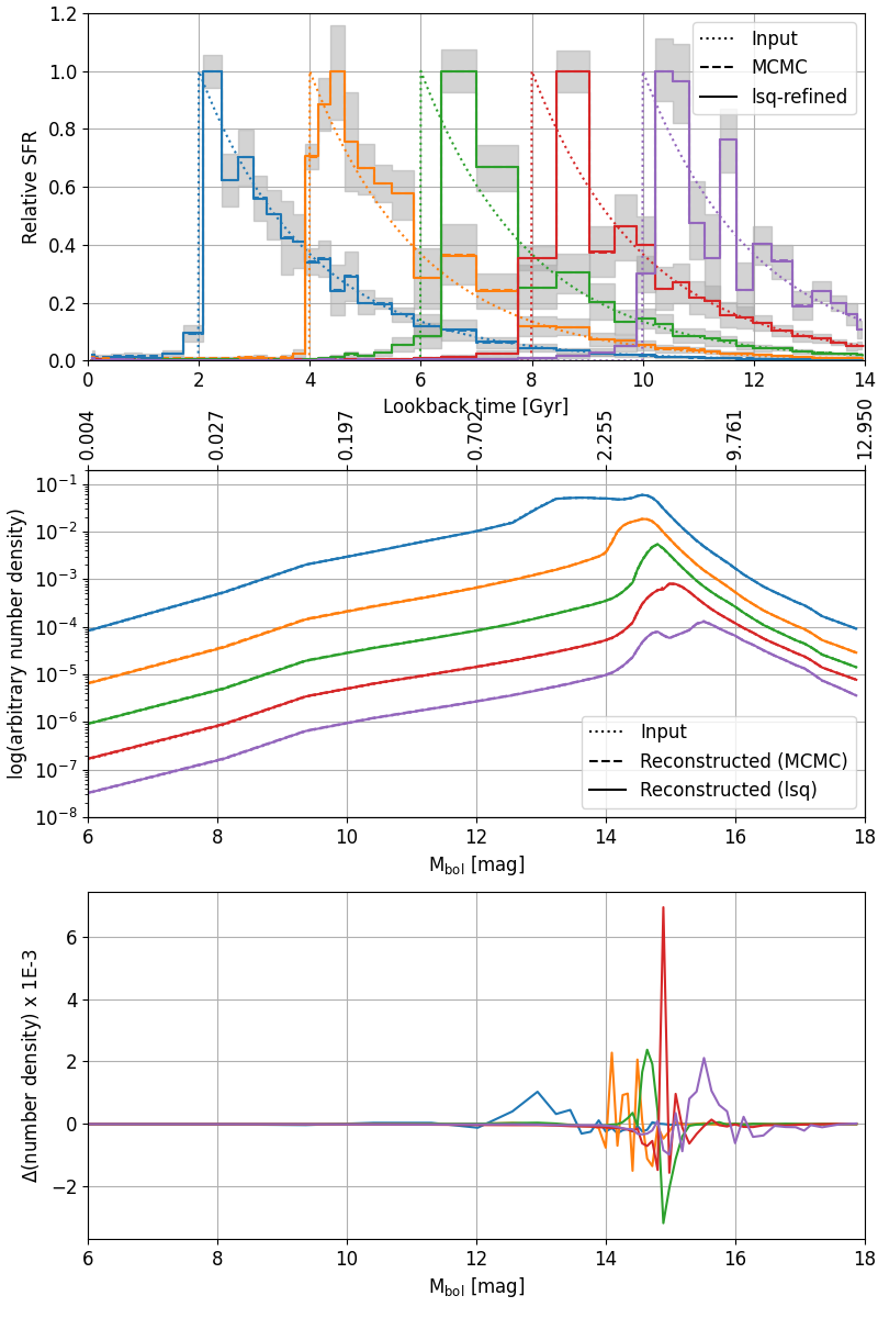
Figure 1: In the top two panels, the input are plotted with dotted line; the marginalized results from the MCMC are plotted with dashed line; and the refined solutions with a least-square minimization method using a set of perturbed MCMC results as initial conditions are plotted in solid lines. The least-squares  (lsq) method is to validate that the solutions are not trapped inside a local minimum. The MCMC and lsq solutions are almost identical. Top: the recovered SFH and reconstructed SFH of a set of mock stellar populations with exponentially increasing star formation rates. Each of the population has an exponential constant of 3 Gyr, the SFHs were truncated at a look-back time of 2, 4, 6, 8, and 10 Gyr. See Section 5.2 for the explanation for the varying bin size in the lookback time. Middle: the input SFHs. Bottom: The difference in the number density between the lsq solution and the input.

Multiple bursts

The set of WDLFs shown in Fig. 2 demonstrates that the method can retrieve both sharp and broad features whether they are distinctly separated or directly on top of each other. The last set (brown) comprises all five sharp peaks and the broad feature. It shows that some correlated results are not completely accounted for at around $6-7$ Gyr (M${}_{\mathrm{bol}}\approx 14-15$ mag). This is coming from the fact that the pWDLFs are very similar as the WDLFs evolve the slowest at these magnitudes, as is obvious from the similarity in the green and red curves in Fig. 2. We plan to address this issue in future work by considering the colour information (see the discussion in Section 7) which should relieve some degeneracy issues in the solutions.

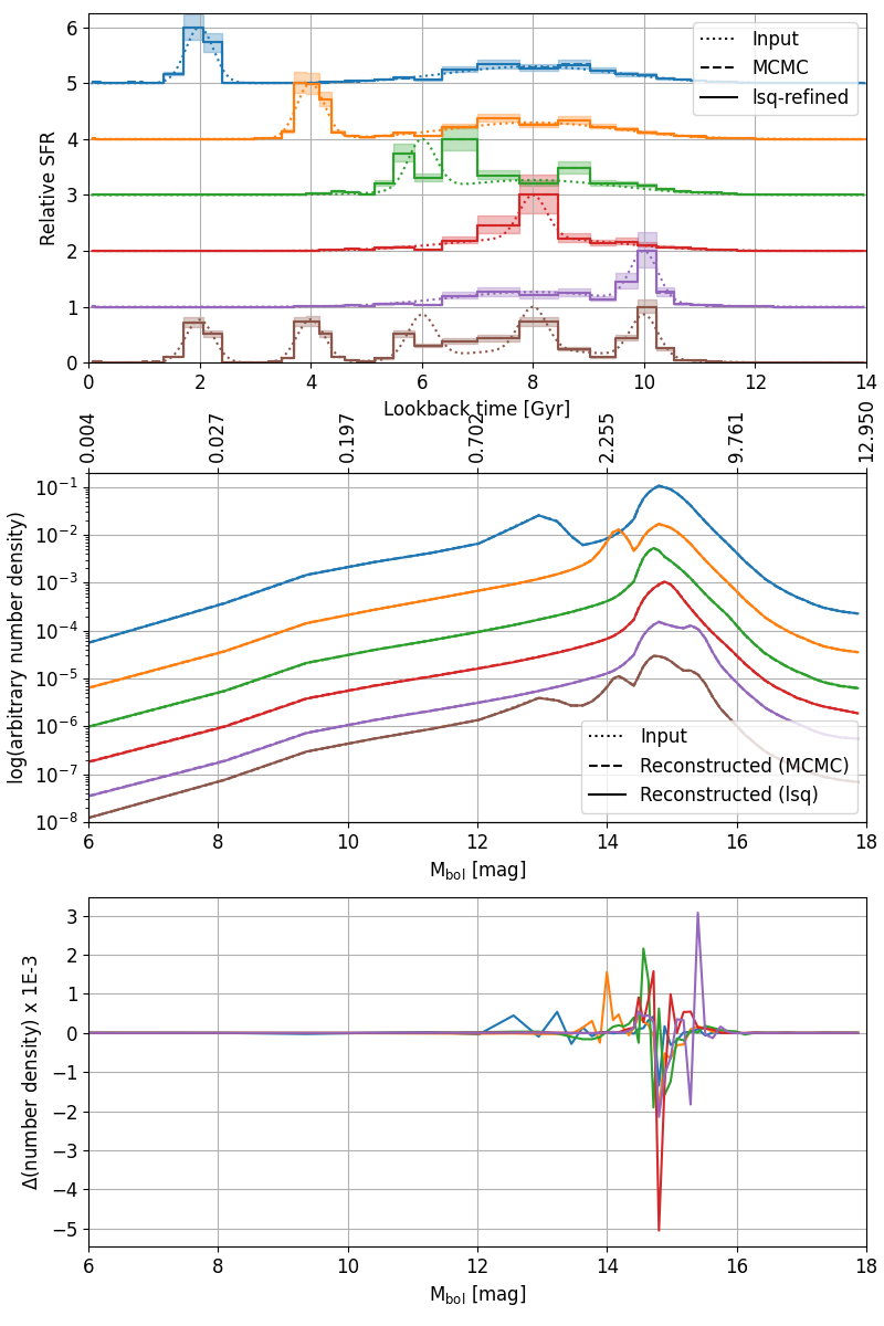
Figure 2: The recovered SFH and reconstructed SFH of a set of mock stellar populations with a dual-burst SFH (blue, orange, green, red and purple), and the last one (brown) is a superposition of five short and one broad SFH. See Fig. 1 for the descriptions of the three sets of legends.

5 Application to the Early Gaia Data Release 3

Upon deriving an SFH from a WDLF, one of the most important unsolved problems is “How much information can we obtain?”. We address in this work how, as a first step, to achieve the maximal sampling in the magnitude space to extract as much information from a WDLF as possible while avoiding the amplification of noise. Any attempt to retrieve a signal at finer intervals than the resolution of the data is essentially amplifying random noise. In this section, we define the optimal bin sizes in bolometric magnitude, and how this naturally defines the lookback time bin sizes.

5.1 WDs from the GCNS

The GCNS contains 21 848 WDs within a 100 pc distance from us. The most significant limitation from this sample is the uncorrected incompleteness. The incompleteness is primarily at the bright end where there are very few WDs, and in the faintest absolute magnitudes where the astrometric solutions are the least reliable due to the intrinsic faintness of these WDs. Furthermore, bright WDs are rare, they are found only at larger distances, there are very few of them in the local 100 pc. The WDs are fitted with the pure hydrogen model from the Montreal group (Bergeron et al., 2019) ignoring the effects of varying the H/He atmospheric composition and surface gravity. The GCNS work interpolated the model grid to look up $G$-band bolometric corrections as a function of ($G-G_{\mathrm{RP}}$) to map M_G to M_bol, at a fixed surface gravity of $\log(g)=8.0$. Because of the different colour evolution as a function of the chemistry of the atmosphere, opting to fit a pure hydrogen atmosphere limits the accuracy of the estimation of the cooling ages as mixed hydrogen-helium atmosphere models give a shorter cooling age than the pure hydrogen model (Bergeron et al., 2022).

When computing the WDLF, the GCNS adopted a fixed scaleheight of 365 pc, a value found from the GCNS itself. This choice can lead to significant effect on the volumetric correction based on the 1/V_max method for deriving the WDLF. Particularly, the scaleheight is increasing with time. However, such evolution is never studied with a completeness corrected sample of WDs (Harris et al., 2006), and previous works on empirical WDLFs all adopted a fixed scaleheight (Harris et al., 2006; Rowell & Hambly, 2011; Lam et al., 2019).

This sample also assumed all WDs have come from isolated stellar evolution, which would be a good assumption given that their colour-absolute magnitude selection and the probability map in the colour-magnitude diagram would have removed WDs at unusually small and large surface gravities. These outliers are products of stars that had gone through stellar interactions in the progenitor systems (e.g.  Ivanova et al., 2013; Hallakoun et al., 2023).

The data available from the GCNS WDLF is a catalogue of WDs where instead of having each row corresponding to one object, each row contributes $1\%$ to the WDLF. When performing photometric fitting of the WDs, the posterior distribution of the distance of each WD is stored for each percentile. Each row represents a $1\%$ chance of the WD at that distance and bolometric magnitude. The catalogue reports the central $99$ percentiles for each WD. The maximum volumes are computed for each percentile for every WD. In some cases, the tail of the distribution exceeds 100 pc (the distance limit of GCNS), these WDs only contribute a small fraction of a WD to the total WDLF. The density normalization and the uncertainties in the WDLF have to be rescaled properly when summing for the total WDLF because directly adding the solution from each row will lead to an amplification of $\sim$$100$ times in the density. Similarly, the error bars would be $100$ times too small if uncorrected. Since the catalogue has retained enough information on the bolometric magnitude and distance, we can choose any bin size to present the GCNS WDLF as it is necessary to optimally extracting the SFH. However, one downside of the catalogue is that it does not come with the uncertainties of the derived bolometric magnitude, so we refit the photometry that has taken into account the photometric and parallactic uncertainties, intrinsic distribution in the surface gravity and the accuracy in using synthetic photometry (see below). In this work, we use the GCNS $M_{\mathrm{bol}}$ and the refitted uncertainties.

5.2 Bin size

From the uncertainties in the photometric fitting for the bolometric magnitudes, we can determine the resolution with which we can sample the WDLF. At the Nyquist sampling rate (Shannon, 1949), there should be two sampling points in the space of one full-width at half maximum (FWHM). Assuming the noise is Gaussian, one FWHM is equivalent to $2.355$ standard deviations ($\sigma$). Thus, the optimal sampling rate is $1.1775\sigma$ at the given magnitude.

5.2.1 Bolometric magnitude

We have identified four main contributions to the uncertainties in the bolometric magnitudes, with which we require to derive the size of the smoothing kernel as a function of the bolometric magnitude.

Uncertainties in the synthetic photometry

The synthetic photometry also comes with uncertainties, we estimate the model uncertainty using the FWHM of the residuals in the SDSS filters reported in Holberg & Bergeron (2006). We take the mean FWHM of in $u$, $g$ and $r$ as the proxy of $G_{\mathrm{BP}}$; the mean FWHM of $u$, $g$, $r$, $i$ and $z$ as a proxy of $G$; and the mean FWHM of $r$, $i$ and $z$ as the proxy of $G_{\mathrm{RP}}$. Dividing them by $2.355$ gives us the dispersion that is added to the Gaia magnitude uncertainty in quadrature. These values are found to be $\sigma_{G_{\mathrm{BP}}}=0.0529$, $\sigma_{G}=0.0462$ and $\sigma_{G_{\mathrm{RP}}}=0.0343$ mag.

Intrinsic distribution of surface gravity

Singly evolved WDs follow a narrow distribution of surface gravity with $\log(g)=7.998\pm 0.011$ for DA (Kepler et al., 2021). An assumption of a fixed surface gravity will lead to a small contribution to the smoothing kernel as it increases the uncertainty.

Uncertainties in photometric fitting

Genest-Beaulieu & Bergeron (2014) reported that photometric fitting with a model grid of synthetic photometry leads to a dispersion of $\sigma_{\log(g)}=0.404$ in the $\log(g)$, which is the combined effect of the intrinsic dispersion and the precision. This is precisely the quantity required in this work because the GCNS sample of WDs was fitted assuming a fixed surface gravity.

Total uncertainties and dispersion

In order to obtain the estimates of the uncertainties in the fitted bolometric magnitudes due to the assumption of fixed surface gravity, we used WDPhotTools to fit the GCNS WD samples in the three Gaia filters at seven surface gravities. These seven values range from $\log(g)-3\sigma_{\log(g)}$ to $\log(g)+3\sigma_{\log(g)}$ in an increment of one $\sigma_{\log(g)}$. The photometric uncertainties in the Gaia filters are the sum in quadrature of the given uncertainties in the photometry in each filter and the corresponding uncertainties in the synthetic photometry (Section 5.2.1 and 5.2.1). While the $\sigma_{\log(g)}$ is the sum in quadrature of the intrinsic distribution of surface gravity and the dispersion in surface gravity coming from photometric fitting  (Section 5.2.1 and 5.2.1).

From the seven fitted bolometric magnitudes, we can approximate the dispersion with:

$$\sigma_{M_{\mathrm{bol}}}=\frac{1}{6}\times\sum_{-3\leq j\leq 3,j\neq 0}\Biggl{\{}\frac{M_{\mathrm{bol}}(\log(g)=7.998+i\sigma_{\log(g)})}{|j|}\\ -M_{\mathrm{bol}}(\log(g)=7.998)\Biggr{\}}$$ (8)

The Gaussian smoothing kernel is described by the sum of the fitting uncertainties, the model uncertainties and the distribution coming from the assumption of fixed surface gravity in quadrature (blue scattered points in top panel of Fig. 3). The weighted average uncertainty as a function of the bolometric magnitude is computed using the inverse maximum volume as weights as it is used to weight each data point to the WDLF.

The use of WDLF relies on the assumption that WD shares similar properties at the same luminosity. Based on such an underlying assumption, we measure the mean of these dispersions weighted by the $1/\mathrm{V}_{\mathrm{max}}$ as provided in the GCNS WD catalogue. Then they are fitted with a spline as a function of bolometric magnitudes (see Fig. 3 and Table 1 in the appendix for the interpolation presented in the middle panel of Fig. 3) to get the average uncertainty as a function of the bolometric magnitude.

5.2.2 Lookback time

The WDLFs with short bursts of star formation are strongly peaked at a single magnitude (see, for example, the set of pWDLFs in Fig. 4). Thus, adding the monotonically cooling nature of WDs, there is a one-to-one mapping of the cooling age of the population and the peak magnitude (see middle panel of Fig. 3). Although at older ages, with the peak magnitude beyond $15$ mag, a WDLF starts to show double peaks, there is always a dominant peak that is at least half an order of magnitude higher in the number density. Thus, we can reliably relate the two relations: peak magnitude–age and peak magnitude–magnitude-resolution. Since the peak magnitude has a one-to-one mapping to the age of the system, we can obtain the time resolution in which we construct the set of the basis pWDLFs that would allow the extraction of the SFH at the maximum sampling rate (i.e. the minimum bin size) without the amplification of noise.

At the oldest age (i.e. faintest magnitudes), the uncertainties of the bolometric magnitude is most likely underestimated as the value $\sigma_{\log(g)}=0.404$ from Genest-Beaulieu & Bergeron (2014) did not include WDs from the faint end. Additionally, from the recent calibration works (Bergeron et al., 2022), it is known that the models are less accurate at the lowest temperature, and the bolometric magnitudes obtained by assuming DA or DB atmosphere is fainter than what mixed hydrogen-helium models would give (Bergeron et al., 2022). However, we cannot quantify these uncertainties, so we only caution readers to pay attention when drawing conclusions from any information fainter than $\approx 15.5$ mag, which corresponds to a look back time of $\approx 9$ Gyr.

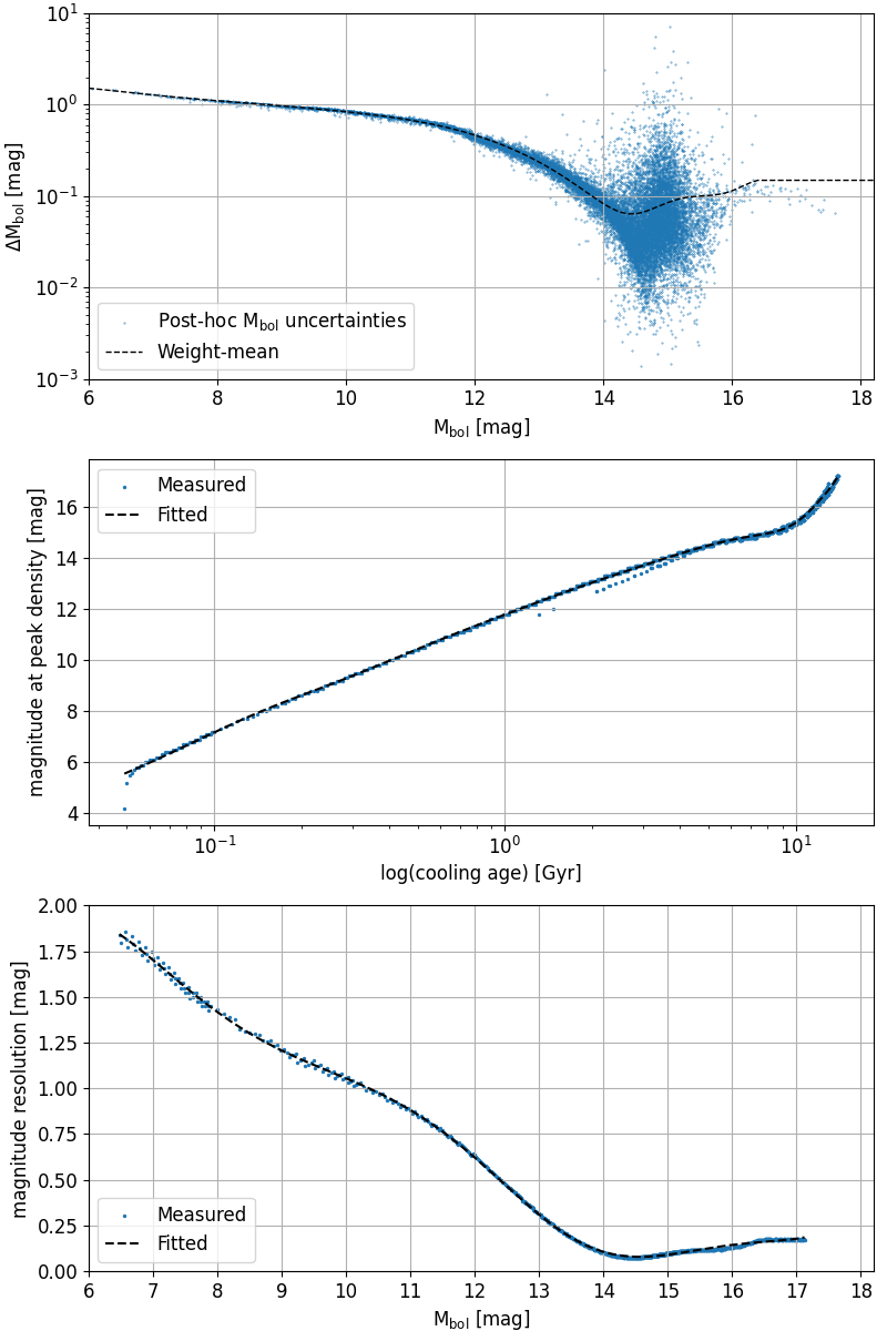
Figure 3: Top: the total uncertainties in the bolometric magnitude as a function of bolometric magnitude (blue). Due to the small number of data points, the weighted average at magnitudes fainter than $16.5$ mag are not computed. At these magnitudes, the uncertainties at the last bin centred at $16.45$ mag is used. Middle: the bolometric magnitude at which the peaks of the pWDLF are located. Bottom: the bolometric magnitude resolution of the WDLF computed using the fitting uncertainties from the top figure and the added uncertainties coming from the synthetic photometry and the assumption of fixed surface gravity (see text). The low resolution in the bright end comes from a combination of large uncertainties in the observed magnitudes, the lack of UV photometry and the sensitivity of the solution to the surface gravity.

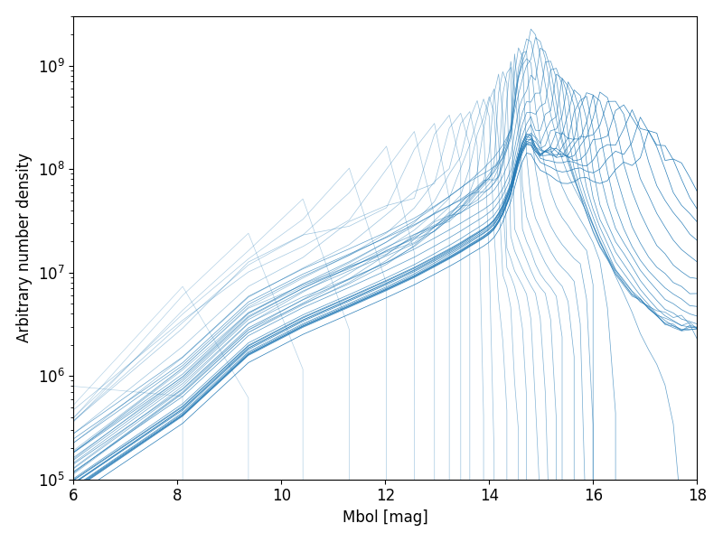
Figure 4: The set of partial WDLF (basis functions) that the peaks are separated by the magnitude resolution as found in Fig 3. At older ages, double peaks start to emerge. However, there is always a dominant peak that is at least half an order of magnitude higher in the contribution. All pWDLFs have the same relative normalization coming directly from the integrations using various input model.

5.3 Star Formation History

By applying the set of basis functions to the fitting method as described in section §4, because the set of pWDLFs is normalized the same way, the relative contribution translates to the relative SFH of the solar neighbourhood. The absolute normalization can be found by matching the reconstructed WDLF to the integrated number density of the input WDLF, and correct for the irregular bin size. We have found multiple phases of enhanced star formation using this novel method, these bursts and lulls are all in good agreement with previous works found using other methods and stellar populations (see Fig. 5 and the next section). We find a strong burst of star formation at $\sim$3 Gyr, and some prominent enhanced star formation at $\sim$2, 4, 9 and 11 Gyr (see bottom panel of Fig. 5)

The 20 pc subset shows the contribution of the WDs within the 20 pc distance, it should not be interpreted as a 20 pc sample where the maximum volume (upper integral limit) for each WD would be different to that of a 100 pc sample. We do not compute the maximum volume in this work, hence we have opted for the word “subset”. We show this subset for a more meaningful comparison of other works that probed much smaller volumes (see Section 6). As already pointed out in the previous section, we caution readers to pay particular attention in drawing conclusions from any information older than $\sim$$9$ Gyr due to, most likely, some correlated signals unaccounted for.

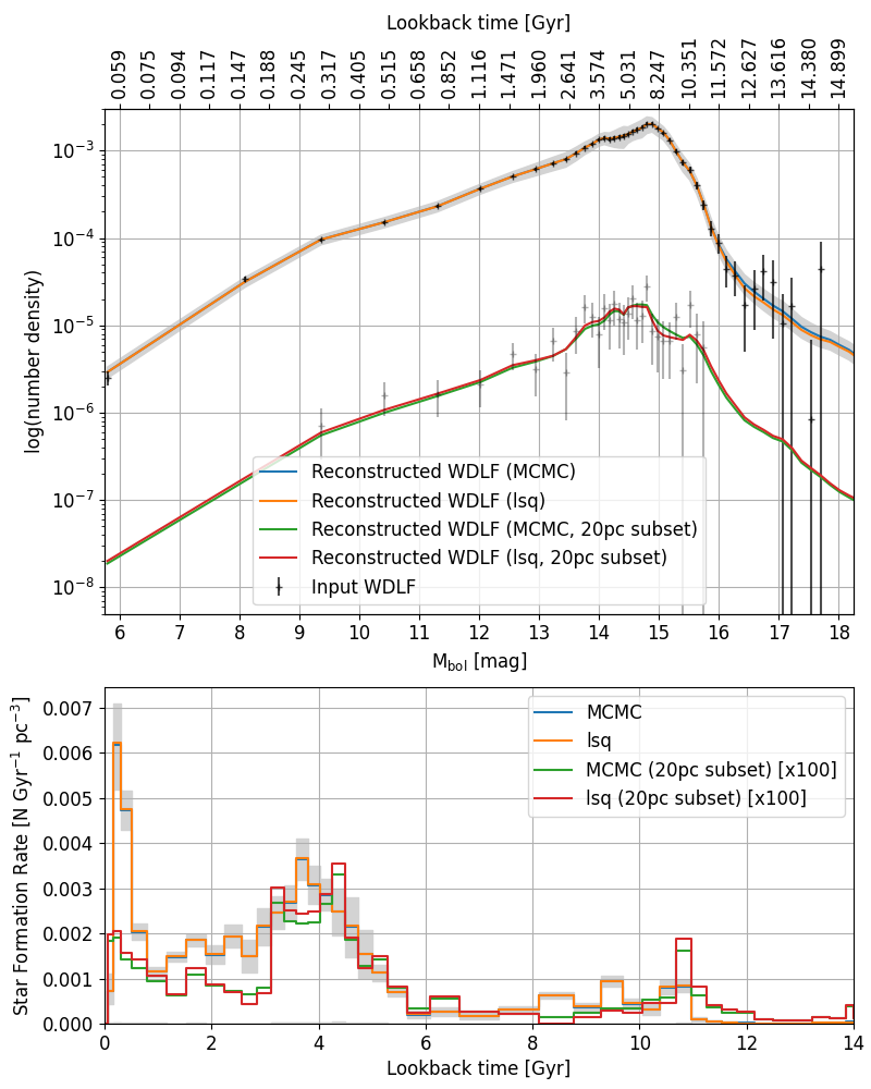
Figure 5: Top: the reconstructed WDLF using MCMC method on the pWDLFs is shown in blue, where the set of solutions is being further refined with a least-squares method is shown in orange. The 20 pc subset shows the contribution of the WDs within the 20 pc distance, it should not be interpreted as a 20 pc sample. The x-axis on the top side shows only the cooling age WDs but not the total age. A luminosity function has marginalized over the progenitor masses, so the total age of WDs is not linearly mapped to the axis of this figure. Bottom: The weights of the pWDLFs transformed to the unit of per billion year by dividing by the bin widths, and by normalizing with the number density to get the unit of per cubic parsec. The raw weights are found from MCMC sampling and finishing with a least-squares minimization.

The tabulated input and best-fit WDLFs from this work can be found in Appendix B.

6 Comparison and discussion

6.1 WDLF

In order to validate the results in this paper, we have compared the resulting SFH with the equivalent result obtained from an independent method applied to the same input WDLF.

Rowell (2013) presented a method to estimate the star formation history from WDLFs using an inversion algorithm on the integral Equation 1. Their method is based on the expectation-maximization algorithm similar in principle to the Richardson-Lucy deconvolution, which is used to obtain maximum-likelihood solutions to inverse problems in the presence of missing data – which in the present application is the unknown distribution of WD mass as a function of magnitude.

We applied their inversion algorithm using an identical set of synthetic photometry to the GCNS dataset to compute the SFH using the same bolometric magnitude binning (see Figure 6). Note that the uncertainty is known to be underestimated, due mostly to the existence of degenerate solutions in the vicinity of rapid changes in star formation rate. Systematic errors arising from e.g. the particular choice of WD cooling models are also not included. The corresponding reconstructed WDLF and residuals are shown in Figure 7.

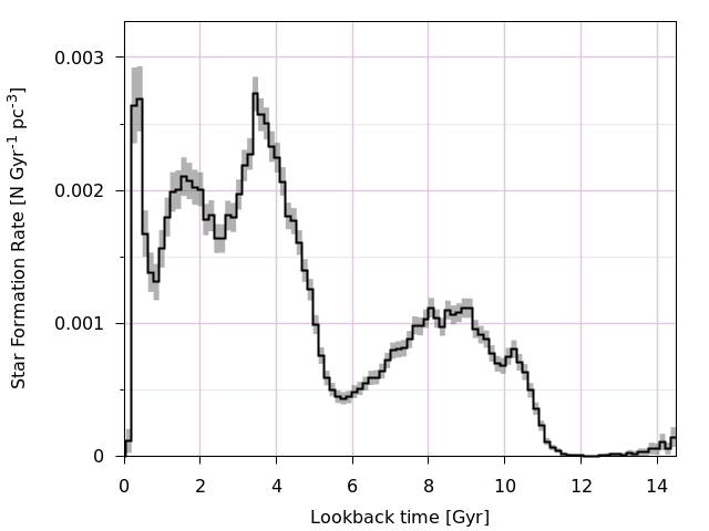
Figure 6: Star formation rate obtained by inversion of the GCNS WDLF using the algorithm presented in Rowell (2013) and described in section 6.1.

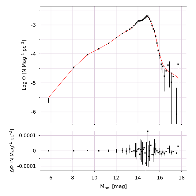
Figure 7: Comparison between the observed (black points) and model (red line) WDLF obtained from the inversion algorithm, and corresponding to the star formation history presented in figure 6.

6.2 Other methods using WDs

T14 reported the SFH using a 20 pc volume-complete sample. They found roughly two broad bursts of SFH. The higher intensity one is in the last 5 Gyr peaking at 3.5 Gyr, and a lower intensity one between 5 and 12 Gyr with a peak at 8.5 Gyr. They are reporting the SFH using the direct number count of WDs, hence further bias corrections are required. The main-sequence bias as termed in T14 is already handled when constructing the WDLF in our case. The kinematics bias is uncorrected in the GCNS sample, and we have not attempted to correct it because in order to perform the correction properly, it has to be computed together in the integral of the maximum volume (Lam et al., 2015). Nevertheless, for a sample that does not require stringent selection criteria, for example, when studying high-velocity WDs only, the kinematic correction is small.

Based on a comparison between T14 and R13, they pointed out a concern regarding the methods of mathematical inversion in the application SFH retrieval from a WDLF. We have shown in Fig. 5 the contribution of SFH from the WDs within a distance of 20 pc that the peak of star formation at a lookback time of about 0.3 Gyr is almost completely disappeared and the SFH is dominated by the broad peak centered at just under 4 Gyr, which is in good agreement with T14. A second broad feature between 8 and 12 Gyr with a sharp peak at 11 Gyr has some resemblance to their findings. The differences, which are mostly a translation and scaling in the direction of the lookback time, are likely to be coming from the adoption of different cooling models. Lam et al. (2022) has illustrated the effect of various models on the shape of the WDLFs. Model combinations C & D in Figure 12 of their work show how the switching between the cooling models including phase separation can lead to a 0.5 mag difference in the position where WDs pile up (due to significant slowdown of the cooling). From Fig. 5, it is clear from the top axis that at these magnitudes, the cooling age is very sensitive to the bolometric magnitude between 13 and 16 mag, corresponding to a cooling age of 1.25 and 9.76 Gyr, respectively, at the two limits.

C23 made use of a similar sample to this work, and they found a constant star formation rate over the last 10.5 Gyr with the 40 pc sample of WDs. Their recovery method overlooks methods available to optimally extract information from a given signal (as we described in details in 5.2). It is possible to identify an optimal bin size and the set of bin sizes determines the time resolution in which we can derive the SFH. In observational astronomy, using photometry as an example, optimal extraction based on a known point-spread function is a technique to maximise the signal-to-noise ratio in the photometry (Tody, 1980; Stetson, 1987). It is possible because we have information on the impulse response of the optical system, including detector effects (and possibly atmospheric seeing). Very similar reasoning is used in, and not limited to, image differencing where a point spread function is used (Alard & Lupton, 1998; Bramich, 2008; Albrow et al., 2009; Zackay et al., 2016), spectroscopy using a line spread function (Horne, 1986; Marsh, 1989; Kelson, 2003), image reconstruction where the smoother kernel is known (Richardson, 1972; Lucy, 1974), and image deconfusion where the position of the two confused sources is known from an external study (Merlin et al., 2015).

Secondly, we attribute the main differences in our derived SFH to their use of chi-squared statistics in fitting cumulative distribution functions (CDF). By fitting a CDF directly to the cumulative data, one would run into significant issues coming from strongly correlated values in the neighbouring values in the ordinal axis. The uncertainty of a data point on a CDF is not merely the uncertainty in that given bin, the uncertainties accumulate to the successive bins non-linearly, depending on how accurate the measurement can be made on the observed variable. In this case, the measurement is the absolute magnitude in the $G$ band. A Poisson error can serve as the lower limit of the uncertainties at best. Specific to fitting a CDF of the bolometric magnitude of WDs, the faintest WDs are most poorly determined because of large uncertainties in both the measurement and in the models. Fitting such CDF with a $\chi^{2}$-minimisation method significantly puts too much weight on the least reliable data. Specifically, the faintest WD has a perfect measurement because a CDF has to converge to unity – a necessary boundary condition.

Thirdly, the scale height they have adopted (75 pc) is much smaller than those adopted by all other WDLF works (e.g. Harris et al. 2006; Rowell & Hambly 2011; Lam et al. 2019). Particularly, Harris et al. (2006) found that the typical minimum and maximum scale height of WD at different bolometric magnitudes span between 200 and 900 pc. C23’s choice of scaleheight is coming from young open clusters, which is not a representative population for the evolution of the galaxy. Given these open clusters remain open clusters by their self-gravity, this value can, at best, set the lower limit of the scaleheight as the progenitor clusters had to have dissolved by the time we observe these isolated WDs. We agree that the youngest WDs should have a smaller scaleheight, and both the scaleheight and $\sigma_{W}$ (velocity dispersion perpendicular to the Galactic plane) increase with time (Rowell & Kilic, 2019). However, assuming both functions increase linearly with time as adopted in their work, the gradients of the two relations are not the same, doubling in $\sigma_{W}$ from 1 to 8 Gyr (Fig. 4 in their work) does not mean the scaleheight doubles over the same time. There is a missing multiplier that should be at least a factor of $\sim$2 to $\sim$3 judging from how the aforementioned works found a typical scale height of $\sim$300 pc. The effect of this missing factor in a simulated population of WDs should lead to an over-density of the older WDs. This can explain the consistent trend of deviation starting at the brightest WD up to $\sim$13 mag (cooling time of $\sim$1 Gyr) because the effect is strongest for the youngest WDs where the scaleheight is comparable to the distance limit of 40 pc, particularly, there is an offset of 20 pc of the Sun from the Galactic plane. Furthermore, the necessary boundary conditions of fitting CDF requires the residuals to converge to 0.0 at the brightest and faintest magnitudes. One should not read it as proof of the quality of fit.

Isern (2019) performed an analysis by directly computing the star formation history of a population of massive WDs selected from Tremblay et al. (2019). The choice of using only massive WDs removes the degeneracy issues arising from the choice of metallicity models of the progenitors; and the fact that massive WDs are remnants of the most massive stars that could have turned into WDs, where their progenitor lifetime is short compared to the WD cooling age. They found an abrupt start of star formation at $\sim$7 Gyr and an enhanced star formation around 2-3 Gyr. They also note that they find a burst at $\sim$0.4 Gyr when applying their method on the 25 pc sample from Oswalt et al. (2017). This recent burst was not seen in all but one previous work – R13’s. Interestingly enough, we have recovered the same peak with the GCNS sample using the R13 inverse modelling method (Section 6.1) and the pWDLF forward modelling method (this work).

Torres et al. (2021) analysed a 100 pc sample of WDs from Torres et al. (2019) with a completeness of $91\%$ at 20.5 mag. This sample contains 95 WDs that are disentangled into thin disk, thick disk and stellar halo components. The data with their selection criteria applied is commonly referred to as a high-velocity sample, but their treatment of the data selection is much more sophisticated, making use of a supervised machine learning method based on Random Forest techniques in eight-dimensional space. They found a cut-off age of $12\pm 0.5$ Gyr where the peak of star formation happened at $\sim$11 Gyr. The star formation continued for about 4 Gyr. $13\%$ of their WDs are younger than 7 Gyr which is puzzling given their kinematic choice, spurious WDs from the thin and thick disk should not have contributed to such a fraction of contamination. They suggested that individual analysis will be required to unravel the origin of these objects.

6.3 MS stars

There are several works concerning the SFH of the solar neighbourhood. We have selected the following three because their sample selections are similar to that of the GCNS sample with little directional dependence.

Cignoni et al. (2006) used the Hipparcos catalogue of stars within 80 PC of the Sun and brighter than $V=8$ mag. The restrictive selection has significantly excluded the effects due to photometric or kinematic incompleteness. They computed the SFH by minimizing the differences between the colour-magnitude diagram of the population from the Hipparcos data and the sum of the partial CMD (the concept that inspired this work to use partial WDLFs). They recovered the strongest star formation at a lookback time of $2-3$ Gyr, and a slowly decreasing SFH up to a lookback time of $6$ Gyr where there is a sharp drop in SFR until a lookback time of $10-12$ Gyr. Their SFH shows excellent agreement to our work, except for the strong peak at the most recent time (see more in Section 7).

Reid et al. (2007) used the Hipparcos catalogue to calibrate bias in the Valenti & Fischer (2005) volume-limited spectroscopic sample of 1 039 FGK dwarfs in the solar neighbourhood with estimates of their age and metallicity. They went through thorough selection criteria, which resulted in two samples. Each sample has limiting absolute magnitudes between $4$ and $\sim$$6$ mag, with a distance limit of $\sim$$30$ pc, and MS mass in the range $\sim 1.25$ to $\sim 0.8$ M_☉. Their results are a direct number count of stars in a volume-limited survey that only include late F to early K stars, so their SFH as plotted in Fig. 8 is a simple normalisation by multiplying by an arbitrary value to allow comparison of the shape, particularly the peaks and troughs of the SFH. The most notable peaks from their work are at $2$ & $4$ Gyr. Two narrow peaks at $6$ & $8$ Gyr are also present.

Bernard (2018) used the TGAS data to perform an initial analysis with the technique of synthetic colour-magnitude diagram-fitting, they found a recent star burst at a lookback time of $\sim$2–3 Gyr, an enhanced star formation $\sim$6–10 Gyr. Figure 8 shows their mildly corrected solutions.

Mor et al. (2019) selected from Gaia DR2 2 890 208 stars with mean $G_{\mathrm{DR2}}<12$, estimated to be $97\%$ complete. Only stars with proxy-absolute magnitude $G_{\pi}$ brighter than $10$ mag are considered in their second filtering in order to remove all brown dwarfs and white dwarfs in their analysis. They applied a non-parametric method that uses an approximate Bayesian computation (Jennings & Madigan, 2017) algorithm to compute their merit function by comparing the Gaia data against the Besancon Galaxy model fast approximation simulations (Mor et al., 2018)). They have found that their analysis is most affected by the thick disk modelling and the stellar evolution models. From their four choices of fitting configurations of the Gaia sample, they see a general trend of decreasing star formation from $\sim$10 Gyr to 6 Gyr, followed by an enhanced star formation of 4 Gyr in duration with a peak at $\sim$2.5 Gyr. They also found a sharp and fast drop in the star formation rate in the most recent 1 Gyr.

6.4 Subgiants

Xiang & Rix (2022) used subgiants to map the metallicity, angular momentum and SFH of the Milky Way. The distance they probe is much larger than this work so it is expected that the recovered SFH shows different features. Nevertheless, they observe one dominant peak at 10.5 Gyr and two small peaks at 2 and 4 Gyr.

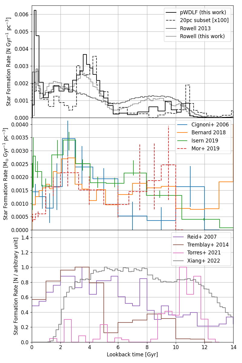
Figure 8: Comparision of the recovered SFH against previous works, see body text of Sec 6 for details. Top: SFH retrieved with the pWDLF method, R13 results (with the H06 WDLF), and the SFH derived using the R13 algorithm on the GCNS WDLF. The 20 pc subset of the GCNS is also plotted for comparison (see body text for details). The SFH is reported in the unit of number of stars formed per unit time per unit volume. Middle: The SFH using four independent methods and samples reported in the unit of solar mass formed per unit time per unit volume (solid line) or projected-area (dashed line). Bottom: The SFHs that are derived from four other independent methods and samples in the unit of number of stars formed per arbitrary time and spatial unit.

7 Conclusions and Future Work

By properly propagating the uncertainties in the systematics and measurements, this work has shown that it is possible to recover the SFH from the WDLF with uncertainties that encompass the uncertainties in the WD atmosphere models, the photometry and the consequence of assuming a fixed surface gravity in the determination of the bolometric magnitude. We have chosen a set of varying bin sizes such that it matches the Nyquist sampling rate where two sampling points are required for every FWHM of the signal. In this case, the single is the shape of the WDLF, which ultimately comes from the SFH. From the comparisons with other works on the SFH of the solar neighbourhood, it is obvious that our new method can retrieve non-parametric SFH. This is achieved by carefully treating the uncertainties from noisy data using well-established mathematical tools. The recovered SFHs agree particularly well at an intermediate age of 0.1-9 Gyr. We outline the most imminent issues to be addressed as follows:

Known issues

1. The GCNS sample is not incompleteness corrected, particularly, the kinematic selection can lead to a significant bias (Tremblay et al., 2014; Lam et al., 2015) in the analysis that leads to underestimation in the number densities. Although not applicable to the GCNS sample, the parallax-related selection usually leads to Lutz-Kelker bias (Lutz & Kelker, 1973), which would affect the shape of the WDLF, hence the SFH.

2. The model uncertainty in the synthetic photometry is considered, however, the treatment is not rigorous as the uncertainty should be a function of the bolometric magnitude. Particularly, it is known that in the visible wavelengths, the errors are the largest in the red end.

3. The properties of the Galaxy are assumed to be static, while in reality the scaleheights and metallicity of the disks and stellar halo have been evolving through cosmic history.

4. There are unaccounted uncertainties from the MS progenitors, including their initial mass function, metallicity evolution, initial-final mass relation, and the binary/multiplicity fraction. All of them can lead to biases in the derived WDLF. As noted by Isern (2019), the R13 method is sensitive to the adopted metallicity and IMF models but not the DA/non-DA ratio and among other choices of models. Although the pWDLF method does not suffer similar convergence and regularisation issues, this method is also sensitive to the choice of MS models, as would any method that requires the progenitor MS lifetimes in the analysis.

5. There are uncertainties from WD modelling that are not considered, for example, the effects from the choice of cooling models, atmosphere models, and synthetic photometric models. Statistical treatment for the bias due to unresolved binaries containing WDs should also be taken into account.

6. There is bias in the bright end of the WDLF leading to the underestimation of the density. Hot WDs can be seen from the largest distance, so they should be the most complete in a 100 pc sample. However, the single scaleheight of 250 pc used in the entire sample of GCNS WDs would lead to a bias. Particularly, as pointed out in C23, the scaleheight of the youngest WDs could be as low as 75 pc.

7. There is incompleteness in the faint end of the sample. It is reported that Gaia has a detection limit of $\sim$20.5 mag. At 100 pc, which corresponds to a distance modulus of 5 mag, an absolute magnitude of $\sim$15.5 mag in $G$ is a naive derivation of the completeness limit. The GCNS contains WDs below this absolute magnitude.

8. In the era of Gaia astrometry, the sample size of WDs is large enough that we should investigate the directional dependency of the WDLFs The CFHS survey (Fantin et al., 2019) and HSC survey (Qiu et al., 2024) seem to reveal a WDLF dissimilar to the WDLFs from SDSS, SuperCOSMOS and Gaia. The distance dependency should also be investigated, since the large distances probed by Gaia (for the relatively bright WDs) means the line-of-sight can go through multiple stellar populations.

When comparing with the T14 sample, we realized that there is a striking difference in the SFH from the 20 pc and 100 pc sample at the most recent time. This brings up three important points that should be investigated: first, arbitrary selection of SFHs reported from different works cannot draw meaningful comparison; second, even at the scale in the order of 10 pc, we can observe variations in the SFHs; third, if the SFH is a strong function of distance from the Sun, then the directional dependency should also be strong given that the Sun is not located in the middle of the Galactic plane. Furthermore, the Sun is not located in the middle of a major arm region of the Galaxy. The analysis should be more complex than simply dividing the sample into zones of Galactic latitudes because, for example, looking into the length of the Orion-Cygnus arm, where the Sun resides, should be different to looking into the inter-arm regions; while the Perseus arm and the Carina-Sagittarius arms are too far away for WD studies, looking into their directions only gives us the WDs in the foreground. In the recent work by Qiu et al. (2024), they have found a much fainter truncation magnitude in the Galactic WDLF using one of the deepest proper-motion and photometry-selected samples to date. Their sample covers a sky area of 165 deg² down to $i=24$ mag. This may be an indication of incompleteness in all previous surveys that have not probed sufficiently deep – methods for completeness correction are not useful when there are no detections at all. Alternatively, it could be due to their assumption that $\sim 90$% of the faintest WDs are members of the thin disc with an exponential scale height of 250 pc, a figure too low for such an old population of stars. This will lead to an underestimation of the generalized survey volume and an overestimation in the spatial density, increased with respect to other surveys that have made similar assumptions due to their significantly increased survey depth.

As pointed out in Mor et al. (2019) and Isern (2019), the decreasing SFR trend from $\sim$10 to 6 Gyr is consistent with the onset of quenching observed in a cosmological context at a redshift of z$\sim$1.8 (corresponds to a lookback time of $\sim$10 Gyr, e.g. Rowan-Robinson et al., 2016; Koprowski et al., 2017). It is also compatible with the evidence of the quenching of the Milky Way (Haywood et al., 2016). This is in line with the thick-disc formation scenario attributed to a major merger event at a lookback time of $\sim$10 Gyr (Helmi et al., 2018).

Beyond systematics and directional dependence, one obvious next step is to use the colour information. All the derivation of SFH from WDLFs of the solar neighbourhood were reported in the bolometric magnitudes/luminosities. Thus, all works have essentially marginalized over the colour-space. To address the problem of degeneracy and correlated signal in the solution, simultaneously fitting multiple WDLFs in various filters may relieve some issues with degeneracy as the pWDLFs evolve at different rates in different wavelengths.

Data Availability

The source code underlying this article, as well as all the data sufficient to reproduce all of the figures in this article are available on GitHub, at https://github.com/cylammarco/SFH-WDLF-article. Two tables are available in the appendix for the magnitude resolution (Fig. 3) and the WDLFs sampled at those magnitude bins (Fig. 5).

Appendix A Tabulated data for the bolometric magnitude resolution

This appendix lists the bin centres and bin sizes used in the WDLFs in this work, as found in Fig. 3.

Magnitude [mag]	Magnitude resolution [mag]
5.7983	3.1967
8.1014	1.4094
9.3663	1.1204
10.4145	0.9759
11.3062	0.8077
12.0220	0.6238
12.5581	0.4485
12.9453	0.3258
13.2311	0.2457
13.4506	0.1935
13.6251	0.1554
13.7680	0.1305
13.8905	0.1146
13.9983	0.1010
14.0934	0.0892
14.1793	0.0826
14.2605	0.0799
14.3388	0.0767
14.4137	0.0731
14.4873	0.0742
14.5621	0.0754
14.6385	0.0774
14.7177	0.0811
14.8009	0.0852
14.8885	0.0899
14.9809	0.0950
15.0784	0.0999
15.1809	0.1051
15.2893	0.1117
15.4018	0.1133
15.5162	0.1154
15.6323	0.1169
15.7504	0.1193
15.8719	0.1236
15.9967	0.1261
16.1279	0.1362
16.2730	0.1541
16.4294	0.1587
16.5881	0.1587
16.7468	0.1587
16.9055	0.1587
17.0642	0.1587
17.2229	0.1587
17.3816	0.1587
17.5403	0.1587

Table 1: The bin centres and bin sizes used as the magnitudes in the WDLFs as found in Fig. 3. The bin sizes are already multiplied by the factor of $2.355/2=1.1775$ as explained in Section 5.2.

Appendix B Tabulated Gaia and reconstructed WDLF

These two tables provide (1) the GCNS WDLF binned at the magnitude as tabulated in Appendix A and the best-fit WDLF and the associated uncertainties from this work; and (2) the same for the 20-pc subset.

Mbol	$\Phi_{\mathrm{GCNS}}$	$\sigma_{\Phi_{\mathrm{GCNS}}}$	$\Phi_{\mathrm{mcmc+lsq}}$	$-\sigma_{\Phi}$	$+\sigma_{\Phi}$
[mag]	[N / Gyr / pc3]		[N / Gyr / pc3]
5.798	2.523414e-06	4.554390e-07	2.915736e-06	0.000000e+00	0.000000e+00
8.101	3.386410e-05	2.526061e-06	3.173625e-05	4.309751e-04	1.103847e-03
9.366	9.520056e-05	4.740354e-06	9.604709e-05	5.185332e-03	7.100745e-03
10.414	1.502980e-04	6.396270e-06	1.510770e-04	4.301908e-03	5.151344e-03
11.306	2.300590e-04	8.687899e-06	2.303309e-04	1.847690e-03	2.222435e-03
12.022	3.649259e-04	1.245546e-05	3.662165e-04	1.047091e-03	1.257641e-03
12.558	5.036294e-04	1.743204e-05	5.046021e-04	1.370802e-03	1.588509e-03
12.945	6.121816e-04	2.233322e-05	6.140492e-04	1.713488e-03	1.989712e-03
13.231	7.119219e-04	2.774027e-05	7.133481e-04	1.328978e-03	1.730608e-03
13.451	7.967154e-04	3.306716e-05	7.990812e-04	1.677853e-03	2.201390e-03
13.625	9.372146e-04	4.005816e-05	9.370679e-04	1.131944e-03	1.860796e-03
13.768	1.080471e-03	4.680300e-05	1.083305e-03	1.733897e-03	2.551980e-03
13.891	1.194054e-03	5.259130e-05	1.193569e-03	2.107802e-03	2.816401e-03
13.998	1.334793e-03	5.919526e-05	1.333824e-03	2.324533e-03	3.073292e-03
14.093	1.383527e-03	6.413906e-05	1.397979e-03	3.177470e-03	4.093294e-03
14.179	1.350647e-03	6.571475e-05	1.367460e-03	2.650060e-03	3.498381e-03
14.261	1.388975e-03	6.859877e-05	1.398500e-03	2.497552e-03	3.212754e-03
14.339	1.421546e-03	7.081691e-05	1.442193e-03	1.963955e-03	2.981955e-03
14.414	1.471563e-03	7.353554e-05	1.482808e-03	1.479573e-03	2.787200e-03
14.487	1.535507e-03	7.437741e-05	1.546505e-03	1.016226e-03	2.071977e-03
14.562	1.662523e-03	7.679106e-05	1.647164e-03	9.457268e-04	1.309049e-03
14.638	1.742285e-03	7.739816e-05	1.735380e-03	6.069240e-04	7.701937e-04
14.718	1.852156e-03	7.792224e-05	1.825555e-03	1.319544e-04	2.827918e-04
14.801	2.025200e-03	7.942008e-05	2.008011e-03	1.801493e-04	3.548753e-04
14.888	2.027768e-03	7.744200e-05	2.016139e-03	1.010963e-04	2.329979e-04
14.981	1.793493e-03	7.093499e-05	1.800859e-03	2.580019e-04	3.829521e-04
15.078	1.593453e-03	6.572193e-05	1.608668e-03	5.457895e-04	7.040109e-04
15.181	1.322591e-03	5.913300e-05	1.313423e-03	2.881408e-04	4.564123e-04
15.289	9.722678e-04	5.107216e-05	9.760354e-04	8.235361e-04	1.050184e-03
15.402	7.298879e-04	4.734546e-05	7.329364e-04	3.203850e-04	5.535021e-04
15.516	6.049411e-04	4.613457e-05	5.839862e-04	1.965852e-04	4.448201e-04
15.632	4.032579e-04	3.994824e-05	4.007261e-04	6.417822e-04	9.671050e-04
15.750	2.381554e-04	3.277612e-05	2.409734e-04	6.978632e-04	9.651653e-04
15.872	1.288113e-04	2.548382e-05	1.327989e-04	5.724355e-05	1.390353e-04
15.997	8.843260e-05	2.335248e-05	8.186839e-05	2.741793e-05	6.911541e-05
16.128	4.461156e-05	1.746933e-05	5.351029e-05	1.628604e-05	4.195098e-05
16.273	3.757578e-05	1.596991e-05	3.762660e-05	9.469341e-06	2.404994e-05
16.429	1.701715e-05	1.197352e-05	2.660023e-05	5.721878e-06	1.311169e-05
16.588	2.609129e-05	1.725264e-05	2.154815e-05	5.227229e-06	1.349627e-05
16.747	4.165517e-05	2.219290e-05	1.827147e-05	6.289489e-06	1.563853e-05
16.906	3.137629e-05	2.436612e-05	1.520276e-05	1.340397e-05	3.276446e-05
17.064	1.047112e-05	1.256871e-05	1.314954e-05	1.140362e-05	2.861901e-05
17.223	1.666423e-05	1.818556e-05	1.081724e-05	2.701836e-05	6.968997e-05
17.382	0.000000e+00	0.000000e+00	8.847148e-06	1.488918e-05	3.629019e-05
17.540	8.376158e-07	5.922987e-06	7.699928e-06	0.000000e+00	0.000000e+00

Table 2: The Gaia WDLFs (left) and the reconstructed WDLFs (middle) in Fig. 5. The uncertainties are only available at the magnitudes when there is observed data. The solutions in bins without observation come from the method fitting partial WDLFs that the faintest WDs are in the model. For a given short period of star burst, the faintest WDs that are unobserved should also be present given the model.

Mbol	$\Phi_{\mathrm{GCNS},20\mathrm{pc}}$	$\sigma_{\Phi_{\mathrm{GCNS},20\mathrm{pc}}}$	$\Phi_{\mathrm{mcmc+lsq},20\mathrm{pc}}$	$-\sigma_{\Phi},20\mathrm{pc}$	$+\sigma_{\Phi},20\mathrm{pc}$
[mag]	[N / Gyr / pc3]		[N / Gyr / pc3]
5.798	0.000000e+00	0.000000e+00	2.008714e-08	0.000000e+00	0.000000e+00
8.101	0.000000e+00	0.000000e+00	1.808817e-07	1.032725e-05	2.613477e-05
9.366	7.002769e-07	4.076263e-07	5.945359e-07	1.295753e-05	2.471377e-05
10.414	1.562234e-06	6.421644e-07	1.075154e-06	8.517363e-06	1.877375e-05
11.306	1.628837e-06	7.338286e-07	1.651998e-06	7.797393e-06	1.586568e-05
12.022	2.115492e-06	9.516867e-07	2.365957e-06	6.177150e-06	1.291882e-05
12.558	4.684087e-06	1.666852e-06	3.492876e-06	3.940791e-06	8.937519e-06
12.945	3.129331e-06	1.576799e-06	3.985347e-06	6.834640e-06	1.559295e-05
13.231	6.557330e-06	2.694735e-06	4.480917e-06	5.306174e-06	1.139134e-05
13.451	2.866976e-06	2.038813e-06	5.351570e-06	4.998281e-06	9.365934e-06
13.625	8.523870e-06	3.835587e-06	7.445907e-06	3.774940e-06	9.276724e-06
13.768	1.634726e-05	5.817472e-06	9.957790e-06	5.336604e-06	1.068174e-05
13.891	1.263226e-05	5.360104e-06	1.089772e-05	1.817502e-05	3.571634e-05
13.998	7.838850e-06	4.553943e-06	1.122371e-05	1.526763e-05	2.962377e-05
14.093	1.572319e-05	6.765451e-06	1.231565e-05	1.272365e-05	3.150949e-05
14.179	1.135261e-05	6.098631e-06	1.437385e-05	1.507442e-05	2.918199e-05
14.261	1.741245e-05	7.475021e-06	1.554368e-05	1.749560e-05	3.481641e-05
14.339	1.183223e-05	6.367848e-06	1.510835e-05	2.103562e-05	4.188097e-05
14.414	1.082799e-05	6.283162e-06	1.339249e-05	1.164923e-05	2.595493e-05
14.487	1.379686e-05	6.950771e-06	1.611393e-05	8.305666e-06	1.743608e-05
14.562	2.037534e-05	8.687685e-06	1.654213e-05	9.932924e-06	1.820051e-05
14.638	1.158530e-05	6.314313e-06	1.658188e-05	4.943371e-06	1.116079e-05
14.718	1.278931e-05	6.429679e-06	1.626148e-05	2.226694e-06	4.627630e-06
14.801	2.804673e-05	9.286878e-06	1.618106e-05	3.684124e-06	7.442626e-06
14.888	8.501000e-06	4.938071e-06	1.144772e-05	1.706969e-06	3.404797e-06
14.981	7.415379e-06	4.502816e-06	8.636473e-06	1.432173e-06	2.876785e-06
15.078	6.693432e-06	4.285507e-06	7.650171e-06	9.704362e-07	2.078141e-06
15.181	6.575534e-06	4.163230e-06	7.330502e-06	1.610019e-06	3.396802e-06
15.289	1.240751e-05	5.661147e-06	7.065039e-06	2.179104e-06	4.427521e-06
15.402	3.033059e-06	3.048347e-06	6.806302e-06	2.087426e-06	4.959924e-06
15.516	1.729959e-05	7.819954e-06	7.810787e-06	3.637352e-06	7.233835e-06
15.632	7.920514e-06	5.749337e-06	6.710100e-06	3.683817e-06	7.783434e-06
15.750	5.611557e-06	5.639829e-06	5.150729e-06	1.058384e-05	2.146752e-05
15.872	0.000000e+00	0.000000e+00	3.406149e-06	3.756867e-06	8.432366e-06
15.997	0.000000e+00	0.000000e+00	2.362102e-06	2.121897e-06	4.946986e-06
16.128	0.000000e+00	0.000000e+00	1.660809e-06	1.659654e-06	3.398983e-06
16.273	0.000000e+00	0.000000e+00	1.225689e-06	1.582272e-06	3.139145e-06
16.429	0.000000e+00	0.000000e+00	8.862513e-07	5.786190e-07	1.190269e-06
16.588	0.000000e+00	0.000000e+00	7.342508e-07	5.460554e-07	1.025725e-06
16.747	0.000000e+00	0.000000e+00	6.372236e-07	4.740149e-07	9.158305e-07
16.906	0.000000e+00	0.000000e+00	5.435278e-07	8.547697e-07	1.861049e-06
17.064	0.000000e+00	0.000000e+00	4.980030e-07	7.937958e-07	1.677031e-06
17.223	0.000000e+00	0.000000e+00	3.947699e-07	2.135516e-06	5.669458e-06
17.382	0.000000e+00	0.000000e+00	2.825303e-07	7.703770e-07	1.566415e-06
17.540	0.000000e+00	0.000000e+00	2.325782e-07	0.000000e+00	0.000000e+00

Table 3: Same as the previous table for the $20$ pc subset.

Appendix C Integration precision requirement

The integration of a WDLF at a given magnitude spans a huge dynamic range in different parameters. In this appendix, we illustrate the importance in setting a sufficient tolerance limit for the integrator such that a continuous WDLF can be generated. This also shows how the precision levels can be computed for a given analysis using theoretical WDLFs.

100 Myr population
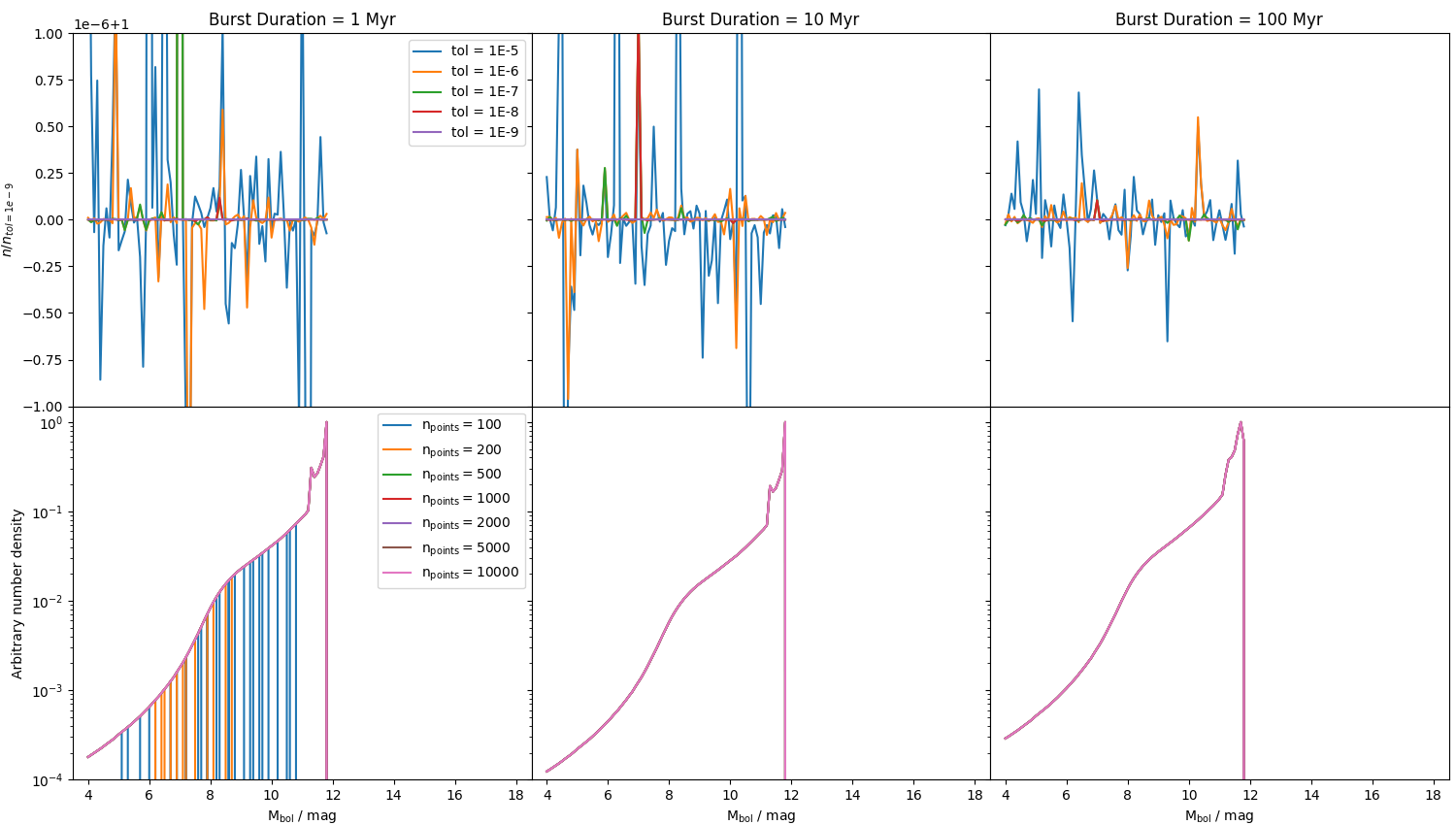
1 Gyr population

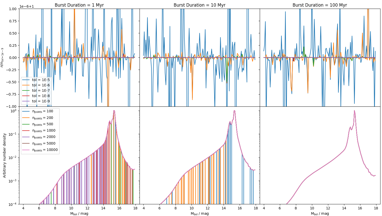
Figure 9: Top: The upper row shows the fractional difference between each of the 100 Myr WDLFs integrated using scipy.integrate.quad with a relative tolerance of $10^{-5}$ (blue), $10^{-6}$ (orange), $10^{-7}$ (green), $10^{-8}$ (red) and $10^{-9}$ (purple) against the WDLF integrated using a relative tolerance of $10^{-9}$, combined with the use of n${}_{\mathrm{points}}=10000$. They are repeated using three different star formation duration, at 1 Myr (left), 10 Myr (middle) and 100 Myr (right). The fractional differences are typically smaller than $10^{-7}$ by using a relative tolerance of $10^{-8}$. The lower row shows the 100 Myr WDLFs integrated using a fixed relative tolerance of $10^{-9}$ and n${}_{\mathrm{points}}=100,200,500,1000,5000$ and $10000$. It is clear that a n_points of at least $500$ is required to compute a WDLF properly. Bottom: Same as above for a 1 Gyr population. The main difference is that for a 1 Myr burst ($0.1\%$ of the age of the population) an n${}_{\mathrm{points}}=5000$ is required to compute a smooth WDLF. Thus, for the partial WDLF we pre-compute in this work, we use a fixed n_points of 10000 and a relative tolerance of $10^{-10}$.

References

- Alard & Lupton (1998) Alard C., Lupton R. H., 1998, ApJ, 503, 325
- Albrow et al. (2009) Albrow M. D., et al., 2009, MNRAS, 397, 2099
- Bailer-Jones et al. (2021) Bailer-Jones C. A. L., Rybizki J., Fouesneau M., Demleitner M., Andrae R., 2021, AJ, 161, 147
- Bédard et al. (2020) Bédard A., Bergeron P., Brassard P., Fontaine G., 2020, ApJ, 901, 93
- Bergeron et al. (2019) Bergeron P., Dufour P., Fontaine G., Coutu S., Blouin S., Genest-Beaulieu C., Bédard A., Rolland B., 2019, ApJ, 876, 67
- Bergeron et al. (2022) Bergeron P., Kilic M., Blouin S., Bédard A., Leggett S. K., Brown W. R., 2022, ApJ, 934, 36
- Bernard (2018) Bernard E. J., 2018, in Recio-Blanco A., de Laverny P., Brown A. G. A., Prusti T., eds, IAU Symposium Vol. 330, Astrometry and Astrophysics in the Gaia Sky. pp 148–151 (arXiv:1801.01427), doi:10.1017/S1743921317006159
- Bramich (2008) Bramich D. M., 2008, MNRAS, 386, L77
- Bressan et al. (2012) Bressan A., Marigo P., Girardi L., Salasnich B., Dal Cero C., Rubele S., Nanni A., 2012, MNRAS, 427, 127
- Cappellari (2023) Cappellari M., 2023, MNRAS, 526, 3273
- Catalán et al. (2008) Catalán S., Isern J., García-Berro E., Ribas I., 2008, MNRAS, 387, 1693
- Chabrier (2003) Chabrier G., 2003, PASP, 115, 763
- Chambers et al. (2016) Chambers K. C., et al., 2016, arXiv e-prints, p. arXiv:1612.05560
- Cignoni et al. (2006) Cignoni M., Degl’Innocenti S., Prada Moroni P. G., Shore S. N., 2006, A&A, 459, 783
- Cukanovaite et al. (2023) Cukanovaite E., Tremblay P. E., Toonen S., Temmink K. D., Manser C. J., O’Brien M. W., McCleery J., 2023, MNRAS, 522, 1643
- Fantin et al. (2019) Fantin N. J., et al., 2019, ApJ, 887, 148
- Gaia Collaboration et al. (2021a) Gaia Collaboration et al., 2021a, A&A, 649, A1
- Gaia Collaboration et al. (2021b) Gaia Collaboration et al., 2021b, A&A, 649, A6