Online ResNet-Based Adaptive Control for Nonlinear Target Tracking

Abstract

This work introduces a generalized ResNet architecture for adaptive control of nonlinear systems with black box uncertainties. The approach overcomes limitations in existing methods by incorporating pre-activation shortcut connections and a zeroth layer block that accommodates different input-output dimensions. The developed Lyapunov-based adaptation law establishes semi-global exponential convergence to a neighborhood of the target state despite unknown dynamics and disturbances. Furthermore, the theoretical results are validated through a comparative simulation.

I Introduction

Neural networks (NNs) are well established for approximating unstructured uncertainties in continuous functions over compact domains [1, 2, 3, 4]. The evolution of NN-based control has progressed from single-layer architectures with Lyapunov-based adaptation [5, 6, 7] to more complex DNN implementations, motivated by numerous examples of improved function approximation efficiency [8, 9, 10]. Early DNN approaches develop Lyapunov-based adaptive update laws for the output layer while the inner layers are updated either in an iterative offline manner as in [11] and [12], or using modular adaptive update laws [13]. Recent developments have established frameworks for real-time adaptation of all DNN layers [14, 15, 16, 17] for various DNN architectures, addressing issues in transient performance [18] and leveraging persistence of excitation [19].

Deep residual neural network (ResNet) architectures have emerged as particularly promising candidates for adaptive control applications. The ResNet architecture is popular because it addresses optimization challenges that arise with increasing network depth, making them potentially valuable for modeling complex system uncertainties.

The key innovation of ResNets is the introduction of skip connections that create direct paths for information to flow through the network during backpropagation as in [20] and [21]. These skip connections help prevent the degradation of gradient information as it passes through multiple layers—a phenomenon known as the vanishing gradient problem where the magnitude of gradients becomes too small for effective weight updates in deep networks. Rather than learning completely new representations at each layer, ResNets learn the difference (or "residual") between the input and the desired output of a layer, which simplifies the optimization process. Theoretical analyses have demonstrated that ResNets possess favorable optimization properties, including smoother loss landscapes [22], absence of spurious local optima with every local minimum being a global minimum as in [23] and [24], and stability of gradient descent equilibria [25]. The universal approximation capabilities of ResNets have also been investigated [26, 27, 28], confirming their ability to approximate any continuous function on a compact set to arbitrary accuracy. A critical advancement in ResNet design was the introduction of pre-activation shortcuts by [29], which position the skip connection before activation functions, improving the flow of information through the network and enhancing the network’s ability to generalize to unseen data. This architectural modification shares conceptual similarities with DenseNets [30], which strengthen feature propagation through dense connectivity patterns that connect each layer to every other layer, facilitating feature reuse and enhancing information flow throughout the network.

Recently, [31] introduced the first Lyapunov-based ResNet for online learning in control applications. However, their implementation utilized the original ResNet architecture without incorporating the pre-activation shortcut connections that have been demonstrated to improve performance [29]. This limitation potentially restricts the learning capabilities and convergence properties of their approach. Additionally, this approach requires the inputs and outputs of the ResNet architecture to be of the same dimensions, thus limiting the applicability of the development. These limitations potentially restrict the learning capabilities and convergence properties of their approach.

In this paper, we develop a generalized ResNet architecture that incorporates pre-activation shortcut connections and a zeroth layer block for target tracking of nonlinear systems. The developed approach positions the skip connection before activation, with post-activation feeding into the DNN block, leveraging the improved information propagation through the network established by [29]. Additionally, the zeroth layer block can compensate for uncertainties with different input and output size, overcoming the limitations of the approaches in [31]. Similar to DenseNets [30], the developed architecture facilitates stronger feature propagation and reuse, and is specifically designed for online learning in control applications. The key contribution of this work is the development and analysis of a Lyapunov-based adaptation law for this generalized ResNet architecture, which establishes semi-global exponential convergence to a neighborhood of the target state despite unknown dynamics and disturbances. Furthermore, the theoretical results are validated through a comparative simulation.

II Deep Residual Neural Network Model

Consider a fully connected feedforward deep residual neural network (ResNet) with $b\in\mathbb{Z}_{\geq 0}$ building blocks, input $x\in\mathbb{R}^{L_{\text{in}}}$, and output $y\in\mathbb{R}^{L_{\text{out}}}$. For each block index $i\in\left\{0,\ldots,b\right\}$, let $k_{i}\in\mathbb{Z}_{>0}$ be the number of hidden layers in the $i^{\text{th}}$ block, let $\kappa_{i}\in\mathbb{R}^{L_{i,0}}$ denote the block input (with $\kappa_{0}\triangleq x$ and $L_{0,0}\triangleq L_{\text{in}}$), and let $\theta_{i}\in\mathbb{R}^{p_{i}}$ be the vector of parameters (weights and biases) associated with the $i^{\text{th}}$ block.

For each block $i\in\left\{0,\ldots,b\right\}$, let $L_{i,j}\in\mathbb{Z}_{>0}$ denote the number of neurons in the $j^{\text{th}}$ layer for $j\in\left\{0,\ldots,k_{i}+1\right\}$. Furthermore, define the augmented dimension $L_{i,j}^{a}\triangleq L_{i,j}+1$, for all $\left(i,j\right)\in\left\{0,\ldots,b\right\}\times\left\{0,\ldots,k_{i}\right\}$. Each block function $\Phi_{i}:\mathbb{R}^{L_{i,0}^{a}}\times\mathbb{R}^{p_{i}}\to\mathbb{R}^{L_{i,k_{i}+1}}$ is a fully connected feedforward deep neural network (DNN), with $L_{i,k_{i}+1}\triangleq L_{\text{out}}$ for all $\left(i,j\right)\in\left\{0,\ldots,b\right\}\times\left\{0,\ldots,k_{i}\right\}$. For any input $v\in\mathbb{R}^{L_{i,j}^{a}}$, the DNN is defined recursively by

$$\varphi_{i,j}\left(v\right)\triangleq\begin{cases}V_{i,0}^{\top}v,&j=0,\\ V_{i,j}^{\top}\phi_{i,j}\left(\varphi_{i,j-1}\left(v\right)\right),&j\in\left\{1,\ldots,k_{i}\right\},\end{cases}$$ (1)

with $\Phi_{i}\left(v,\theta_{i}\right)=\varphi_{i,k_{i}}\left(v\right)$.

For each $j\in\left\{0,1,\ldots,k_{i}\right\}$ the matrix $V_{i,j}\in\mathbb{R}^{L_{i,j}^{a}\times L_{i,j+1}}$ contains the weights and biases; in particular, if a layer has $n$ (augmented) inputs and the subsequent layer has $m$ nodes, then $V\in\mathbb{R}^{n\times m}$ is constructed so that its $\left(i,j\right)^{\text{th}}$ entry represents the weight from the $i^{\text{th}}$ node of the input to the $j^{\text{th}}$ node of the output, with the last row corresponding to the bias terms. For the DNN architecture described by (1), the vector of DNN weights of the $i^{\text{th}}$ block is $\theta_{i}\triangleq\left[\begin{array}[]{ccc}\text{vec}\left(V_{i,0}\right)^{\top}&\cdots&\text{vec}\left(V_{i,k_{i}}\right)^{\top}\end{array}\right]^{\top}\in\mathbb{R}^{p_{i}}$, where $p_{i}\triangleq\sum_{j=0}^{k_{i}}L_{i,j}^{a}L_{i,j+1}$, and $\text{vec}\left(V_{i,j}\right)$ denotes the vectorization of $V_{i,j}$ performed in column-major order (i.e., the columns are stacked sequentially to form a vector). The activation function $\phi_{i,j}:\mathbb{R}^{L_{i,j}}\to\mathbb{R}^{L_{i,j}^{a}}$ is given by $\phi_{i,j}\left(\varphi_{i,j-1}\right)$ $=$ $\left[\varsigma_{i,1}\left(\left(\varphi_{i,j-1}\right)_{1}\right)\right.$ $\begin{array}[]{c}\varsigma_{i,2}\left(\left(\varphi_{i,j-1}\right)_{2}\right)\end{array}$ $\begin{array}[]{c}\cdots\end{array}$ $\begin{array}[]{c}\varsigma_{i,L_{i,j}}\left(\left(\varphi_{i,j-1}\right)_{L_{i,j}}\right)\end{array}$ $\left.1\right]^{\top}$ $\in\mathbb{R}^{L_{i,j}^{a}}$ where $\left(\varphi_{i,j-1}\right)_{\ell}$ denotes the $\ell^{\text{th}}$ component of $\varphi_{i,j-1}$, each $\varsigma_{i,j}:\mathbb{R}\to\mathbb{R}$ denotes a smooth activation function, and 1 denotes the augmented hidden layer that accounts for the bias term.

Figure 1: Deep Residual Neural Network Architecture

A pre-activation design is used so that, before each block (except block $0$), the output of the previous block is processed by an external activation function. Specifically, for each block $i\in\left\{1,\ldots,b\right\}$, define the pre-activation mapping $\psi_{i}:\mathbb{R}^{L_{i,k_{i}+1}}\to\mathbb{R}^{L_{i,k_{i}+1}^{a}}$ by $\psi_{i}\left(\kappa_{i}\right)$ $=$ $\left[\varrho_{i,1}\left(\left(\kappa_{i}\right)_{1}\right)\right.$ $\varrho_{i,2}\left(\left(\kappa_{i}\right)_{2}\right)$ $\begin{array}[]{c}\cdots\end{array}$ $\varrho_{i,L_{i,k_{i}+1}}\left(\left(\kappa_{i}\right)_{L_{i,k_{i}+1}}\right)$ $\left.1\right]^{\top}$ $\in\mathbb{R}^{L_{i,k_{i}+1}^{a}}$ where $\left(\kappa_{i}\right)_{\ell}$ denotes the $\ell^{\text{th}}$ component of $\kappa_{i}$, each $\varrho_{i,j+1}:\mathbb{R}\to\mathbb{R}$ denotes a smooth activation function, and 1, again, accounts for the bias term. The output of $\psi_{i}$ serves as the input to block $i$ and the residual connection is implemented by adding the current block output to the pre-activated output from the previous block. Hence, the ResNet recursion is defined by

$$\kappa_{i+1}\triangleq\begin{cases}\Phi_{0}\left(\kappa_{0}^{a},\theta_{0}\right),&i=0,\\ \kappa_{i}+\Phi_{i}\left(\psi_{i}\left(\kappa_{i}\right),\theta_{i}\right),&i\in\left\{1,\ldots,b\right\},\end{cases}$$ (2)

with output $y\in\mathbb{R}^{L_{\text{out}}}$ and overall parameter vector $\Theta\triangleq\left[\begin{array}[]{ccc}\theta_{0}&\cdots&\theta_{b}\end{array}\right]\in\mathbb{R}^{{\tt p}}$, with ${\tt p}\triangleq\sum_{i=0}^{b}p_{i}$, where $\kappa_{0}^{a}\triangleq\left[\begin{array}[]{cc}\kappa_{0}^{\top}&1\end{array}\right]^{\top}\in\mathbb{R}^{L_{0,0}^{a}}$ denotes the augmented input to block $i=0$. Therefore, the complete ResNet is represented as $\Psi:\mathbb{R}^{L_{\text{in}}}\times\mathbb{R}^{{\tt p}}\to\mathbb{R}^{L_{\text{out}}}$ expressed as $\Psi\left(\kappa,\Theta\right)=\kappa_{b+1}$.

The Jacobian of the ResNet is represented as $\frac{\partial}{\partial\Theta}\Psi\left(\kappa,\Theta\right)=\left[\begin{array}[]{ccc}\frac{\partial}{\partial\theta_{0}}\Psi\left(\kappa,\Theta\right)&\cdots&\frac{\partial}{\partial\theta_{b}}\Psi\left(\kappa,\Theta\right)\end{array}\right]\in\mathbb{R}^{L_{\text{out}}\times{\tt p}}$ and $\frac{\partial}{\partial\theta_{i}}\Psi\left(\kappa,\Theta\right)=\left[\begin{array}[]{ccc}\frac{\partial}{\partial{\rm vec}\left(V_{i,0}\right)}\Psi\left(\kappa,\Theta\right)&\cdots&\frac{\partial}{\partial{\rm vec}\left(V_{i,k_{i}}\right)}\Psi\left(\kappa,\Theta\right)\end{array}\right]\in\mathbb{R}^{L_{\text{out}}\times p_{i}}$, where $\frac{\partial}{\partial{\rm vec}\left(V_{i,j}\right)}\Psi\left(\kappa,\Theta\right)\in\mathbb{R}^{L_{\text{out}}\times L_{i,j}^{a}L_{i,j+1}}$ for all $j\in\left\{0,\ldots,k_{i}\right\}$. Using (1), (2), and the property of the vectorization operator yields

$$\frac{\partial\Psi}{\partial\mathrm{vec}\left(V_{i,j}\right)} =\left(\stackrel{{\scriptstyle\curvearrowleft}}{{\stackrel{{\scriptstyle[}}{{m}}=i+1]{b}{\prod}}}\left(I_{L_{\text{out}}}+\left(\stackrel{{\scriptstyle\curvearrowleft}}{{\stackrel{{\scriptstyle[}}{{\ell}}=1]{k_{m}}{\prod}}}V_{m,\ell}^{\top}\frac{\partial\phi_{m,\ell}}{\partial\varphi_{m,\ell-1}}\right)V_{m,0}^{\top}\frac{\partial\psi_{m}}{\partial\kappa_{m}}\right)\right)$$

$$\hskip 7.00002pt\cdot\left(\stackrel{{\scriptstyle\curvearrowleft}}{{\stackrel{{\scriptstyle[}}{{\ell}}=j+1]{k_{i}}{\prod}}}V_{i,\ell}^{\top}\frac{\partial\phi_{i,\ell}}{\partial\varphi_{i,\ell-1}}\right)\left(I_{L_{i,j+1}}\otimes\varkappa_{i,j}^{\top}\right),$$

where $\varkappa_{i,j}\triangleq\mathbf{1}_{\left\{i=0\right\}}\left(\kappa_{0}^{a}\mathbf{1}_{\left\{j=0\right\}}+\phi_{0,j}\left(\varphi_{0,j-1}\left(\kappa_{0}^{a}\right)\right)\mathbf{1}_{\left\{j>0\right\}}\right)$ $+$ $\mathbf{1}_{\left\{i>0\right\}}\left(\psi_{i}\left(\kappa_{i}\right)\mathbf{1}_{\left\{j=0\right\}}+\phi_{i,j}\left(\varphi_{i,j-1}\left(\psi_{i}\left(\kappa_{i}\right)\right)\right)\mathbf{1}_{\left\{j>0\right\}}\right)$ for $\left(i,j\right)\in\left\{0,\ldots,b\right\}\times\left\{0,\ldots,k_{i}\right\}$.

The Jacobian $\frac{\partial\phi_{i,j}\left(\varphi_{i,j-1}\left(v\right)\right)}{\partial\varphi_{i,j-1}\left(v\right)}:\mathbb{R}^{L_{i,j}}\to\mathbb{R}^{L_{i,j}^{a}\times L_{i,j}}$ of the activation function vector at the $j^{\mathrm{th}}$ layer is given by $\frac{\partial\phi_{i,j}\left(\varphi_{i,j-1}\left(v\right)\right)}{\partial\varphi_{i,j-1}\left(v\right)}$ $=$ $\left[\text{diag}\left\{\frac{{\rm d}\varsigma_{i,1}\left(\left(\varphi_{i,j-1}\right)_{1}\right)}{{\rm d}\left(\varphi_{i,j-1}\right)_{1}},\ldots,\frac{{\rm d}\varsigma_{i,L_{i,j}}\left(\left(\varphi_{i,j-1}\right)_{L_{i,j}}\right)}{{\rm d}\left(\varphi_{i,j-1}\right)_{L_{i,j}}}\right\}\right.$$\left.\mathbf{0}_{L_{i,j}}^{\top}\right]^{\top}$. Similarly, the Jacobian $\frac{\partial\psi_{m}\left(\kappa_{m}\right)}{\partial\kappa_{m}}:\mathbb{R}^{L_{\text{out}}}\to\mathbb{R}^{L_{\text{out}}^{a}\times L_{\text{out}}}$ of the pre-activation function vector at block $m$ is given by $\frac{\partial\psi_{m}\left(\kappa_{m}\right)}{\partial\kappa_{m}}$ $=$ $\left[\text{diag}\left\{\frac{{\rm d}\varrho_{m,1}\left(\left(\kappa_{m}\right)_{1}\right)}{{\rm d}\left(\kappa_{m}\right)_{1}},\ldots,\frac{{\rm d}\varrho_{m,L_{\text{out}}}\left(\left(\kappa_{m}\right)_{L_{\text{out}}}\right)}{{\rm d}\left(\kappa_{m}\right)_{L_{\text{out}}}}\right\}\right.$$\left.\mathbf{0}_{L_{\text{out}}}^{\top}\right]^{\top}$.

III Problem Formulation

Consider the second order nonlinear system

$$\ddot{q}=f\left(q,\dot{q}\right)+g\left(q,\dot{q},t\right)u+\omega\left(t\right),$$ (3)

where $q,\dot{q}\in\mathbb{R}^{n}$ denote the known generalized position and velocity, respectively, $\ddot{q}\in\mathbb{R}^{n}$ denotes the unknown generalized acceleration, the unknown functions $f:\mathbb{R}^{n}\times\mathbb{R}^{n}\to\mathbb{R}^{n}$ and $\omega:\left[0,\infty\right)\to\mathbb{R}^{n}$ represent modeling uncertainties and exogenous disturbances, respectively, $g:\mathbb{R}^{n}\times\mathbb{R}^{n}\times\left[0,\infty\right)\to\mathbb{R}^{n\times m}$ denotes the known control effectiveness matrix, and $u\in\mathbb{R}^{m}$ denotes the control input. Here, the function $f$ is of class ${\tt C}^{1}$, the function $g$ has full row-rank, is of class ${\tt C}^{1}$, the mapping $t\mapsto g\left(q,\dot{q},t\right)$ is uniformly bounded, the function $\omega$ is of class ${\tt C}^{1}$, and there exists a known constant $\overline{\omega}\in\mathbb{R}_{\geq 0}$ such that $\left\|\omega\left(t\right)\right\|\leq\overline{\omega}$ for all $t\in\left[0,\infty\right)$. By the full row-rank property, the existence of the right Moore-Penrose inverse $g^{+}:\mathbb{R}^{n}\times\mathbb{R}^{n}\times\left[0,\infty\right)\to\mathbb{R}^{m\times n}$ is guaranteed, defined as $g^{+}\left(\cdot\right)\triangleq g^{\top}\left(\cdot\right)\left(g\left(\cdot\right)g^{\top}\left(\cdot\right)\right)^{-1}$, where the function $g^{+}$ is of class ${\tt C}^{1}$ and the mapping $t\mapsto g^{+}\left(q,\dot{q},t\right)$ is uniformly bounded. The dynamics for the target trajectory are given by

$$\ddot{q}_{d}=f_{d}\left(q_{d},\dot{q}_{d}\right),$$ (4)

where $q_{d},\dot{q}_{d}\in\mathbb{R}^{n}$ denote the measurable generalized position and velocity, respectively, $\ddot{q}_{d}\in\mathbb{R}^{n}$ denotes the unknown generalized acceleration, and the unknown function $f_{d}:\mathbb{R}^{n}\times\mathbb{R}^{n}\to\mathbb{R}^{n}$ represents the unknown target drift.

Assumption 1.

There exist known constants $\overline{q}_{d},\overline{\dot{q}}_{d}\in\mathbb{R}_{>0}$ such that $\left\|q_{d}\left(t\right)\right\|\leq\overline{q}_{d}$ and $\left\|\dot{q}_{d}\left(t\right)\right\|\leq\overline{\dot{q}}_{d}$ for all $t\in\left[0,\infty\right)$.

The control objective is to design a ResNet-based adaptive controller such that the state $q$ is exponentially regulated to a neighborhood of the target state $q_{d}$, despite the presence of unknown dynamics and disturbances. To facilitate the tracking objective, let the tracking error $e\in\mathbb{R}^{n}$ be defined as

$$e\triangleq q_{d}-q.$$ (5)

IV Control Synthesis

To facilitate the control design, let the auxiliary tracking error $r\in\mathbb{R}^{n}$ be defined as

$$r\triangleq\dot{e}+k_{1}e,$$ (6)

where $k_{1}\in\mathbb{R}_{>0}$ denotes a constant control gain. Substituting (3)-(6) into the time-derivative of (6) yields

$$\dot{r}=h\left(q,\dot{q},q_{d},\dot{q}_{d}\right)-g\left(q,\dot{q},t\right)u-\omega\left(t\right)+k_{1}\left(r-k_{1}e\right),$$ (7)

where $h\left(q,\dot{q},q_{d},\dot{q}_{d}\right)\triangleq f_{d}\left(q_{d},\dot{q}_{d}\right)-f\left(q,\dot{q}\right)$.

IV-A Residual Neural Network Function Approximation

The ResNet architecture, defined by skip connections and hierarchical feature extraction, learns the differences (or "residuals") between the input and desired output at each layer, effectively modeling incremental changes rather than complete transformations of nonlinear dynamical systems without requiring explicit governing equations. This approach simplifies the learning task by focusing on how much the representation needs to change at each stage rather than learning entirely new representations. This approximation capability addresses systems with high-dimensional state spaces, nonlinearities, and coupling effects that conventional physics-based models cannot adequately represent. The integration of ResNet-based function approximation into system identification and control frameworks enables the development of models for nonlinear dynamical systems with formal approximation error bounds under appropriate regularity conditions.

To facilitate the tracking objective, a ResNet will be used to approximate the unknown dynamics given by $h\left(q,\dot{q},q_{d},\dot{q}_{d}\right)$ in (7). Let $\kappa\triangleq\left[\begin{array}[]{cccc}q^{\top}&\dot{q}^{\top}&q_{d}^{\top}&\dot{q}_{d}^{\top}\end{array}\right]^{\top}\in\Omega$ denote the known input to the ResNet, where $\Omega\subset\mathbb{R}^{4n}$ denotes the compact set over which the universal approximation property holds. The ResNet-based approximation of $h\left(\kappa\right)$ is given by $\widehat{h}=\Psi\left(\kappa,\widehat{\Theta}\right)$, where $\Psi:\mathbb{R}^{4n}\times\mathbb{R}^{{\tt p}}\to\mathbb{R}^{n}$ denotes the ResNet architecture and $\widehat{\Theta}\in\mathbb{R}^{{\tt p}}$ denotes the ResNet parameter estimates that are subsequently designed. The approximation objective is to determine optimal estimates of $\widehat{\Theta}$ such that $\kappa\mapsto\Psi\left(\kappa,\widehat{\Theta}\right)$ approximates $\kappa\mapsto h\left(\kappa\right)$ with minimal error for any $\kappa\in\Omega$. To quantify the approximation objective, let the loss function $\mathcal{L}:\mathbb{R}^{{\tt p}}\to\mathbb{R}_{\geq 0}$ be defined as

$$\mathcal{L}\left(\Theta\right)\triangleq\int_{\Omega}\left(\left\|h\left(\kappa\right)-\Psi\left(\kappa,\Theta\right)\right\|^{2}+\sigma\left\|\Theta\right\|^{2}\right){\rm d}\mu\left(\kappa\right),$$ (8)

where $\mu$ denotes the Lebesgue measure, $\sigma\in\mathbb{R}_{>0}$ denotes a regularizing constant, and the term $\sigma\left\|\Theta\right\|^{2}$ represents $L_{2}$ regularization. Let $\mathbb{f}\subset\mathbb{R}^{{\tt p}}$ denote a user-selected compact, convex parameter search space with a smooth boundary, satisfying $\mathbf{0}_{{\tt p}}\in\text{int}\left(\mathbb{f}\right)$. Additionally, define $\overline{\Theta}\triangleq\underset{\Theta\in\mathbb{f}}{\max}\left\|\Theta\right\|.$ Due to the strict convexity of the regularizing term $\sigma\left\|\Theta\right\|^{2}$ in (8), there exists $\sigma\in\mathbb{R}_{>0}$ which ensures $\mathcal{L}\left(\Theta\right)$ is convex for all $\Theta\in\mathbb{f}$. For ResNets with arbitrary nonlinear activation functions, it has been established that every local minimum is a global minimum [24]. The objective is to identify the vector of ideal ResNet parameters $\Theta^{\ast}\in\mathbb{f}$ defined as

$$\Theta^{\ast} \triangleq \underset{\Theta\in\mathbb{f}}{\arg\min\ }\mathcal{L}\left(\Theta\right).$$ (9)

For clarity in subsequent analysis, it is desirable that the solution $\Theta^{\ast}$ to (9) be unique. To this end, the following assumption is made.

Assumption 2.

The loss function $\mathcal{L}$ is strictly convex over the set $\mathbb{f}$.

Remark 1.

The universal function approximation property of ResNets was not invoked in the definition of $\Theta^{\ast}$. The universal function approximation theorem states that the function space of ResNets is dense in the space of continuous functions ${\tt C}\left(\Omega\right)$ [26, 28]. Consequently, for any prescribed $\overline{\varepsilon}>0$, there exists a ResNet $\Psi$ and a corresponding parameter $\Theta$ such that $\underset{\kappa\in\Omega}{\sup}\left\|h\left(\kappa\right)-\Psi\left(\kappa,\Theta\right)\right\|<\overline{\varepsilon}$, and therefore $\int_{\Omega}\left\|h\left(\kappa\right)-\Psi\left(\kappa,\Theta\right)\right\|^{2}{\rm d}\mu\left(\kappa\right)<\overline{\varepsilon}^{2}\mu\left(\Omega\right)$. However, determining a search space $\mathbb{f}$ for arbitrary $\overline{\varepsilon}$ remains an open challenge. Therefore, $\mathbb{f}$ is allowed to be arbitrarily selected, at the expense of guarantees on the approximation accuracy.

IV-B Control Design

Following the previous discussion, the unknown dynamics in (7) can be modeled using a ResNet as

$$h\left(\kappa\right)=\Psi\left(\kappa,\Theta^{\ast}\right)+\varepsilon\left(\kappa\right),$$ (10)

where $\varepsilon:\mathbb{R}^{4n}\to\mathbb{R}^{n}$ is an unknown function representing the reconstruction error that is bounded as

$$\sup_{\kappa\in\Omega}\left\|\varepsilon\left(\kappa\right)\right\|<\overline{\varepsilon}.$$ (11)

Based on (7) and the subsequent stability analysis, the control input is designed as

$$u=g^{+}\left(q,\dot{q},t\right)\left(\left(1-k_{1}^{2}\right)e+\left(k_{1}+k_{2}\right)r+\Psi\left(\kappa,\widehat{\Theta}\right)\right),$$ (12)

where $k_{2}\in\mathbb{R}_{>0}$ denotes a constant control gain. Substituting (10) and (12) into (7) yields

$$\dot{r}=-k_{2}r-e+\Psi\left(\kappa,\Theta^{\ast}\right)-\Psi\left(\kappa,\widehat{\Theta}\right)+\varepsilon\left(\kappa\right)-\omega\left(t\right).$$ (13)

Based on the subsequent stability analysis, the adaptive update law is designed as

$$\dot{\widehat{\Theta}}=\text{proj}\left(\Gamma\left(\frac{\partial\Psi\left(\kappa,\widehat{\Theta}\right)}{\partial\Theta}^{\top}r-k_{3}\widehat{\Theta}\right)\right),$$ (14)

where $k_{3}\in\mathbb{R}_{>0}$ denotes a constant control gain, $\Gamma\in\mathbb{R}^{{\tt p}\times{\tt p}}$ is a user-defined positive definite learning rate, and where the projection operator ensures $\widehat{\Theta}\left(t\right)\in\mathbb{f}$ for all $t\in\mathbb{R}_{\geq 0}$, defined as in [32, Appendix E].

V Stability Analysis

The ResNet described in (10) is inherently nonlinear with respect to its weights. Designing adaptive controllers and performing stability analyses for systems that are nonlinearly parameterizable presents significant theoretical challenges. A method to address the nonlinear structure of the uncertainty, especially for ResNets, is to use a first-order Taylor series approximation. To quantify the approximation, the parameter estimation error $\widetilde{\Theta}\in\mathbb{R}^{{\tt p}}$ is defined as

$$\widetilde{\Theta}=\Theta^{\ast}-\widehat{\Theta}.$$ (15)

Applying first-order Taylor’s theorem to $\Psi\left(\kappa,\Theta^{\ast}\right)$ evaluated at $\widehat{\Theta}$ and using (15) yields

$$\Psi\left(\kappa,\Theta^{\ast}\right)-\Psi\left(\kappa,\widehat{\Theta}\right)=\frac{\partial}{\partial\widehat{\Theta}}\Psi\left(\kappa,\widehat{\Theta}\right)\widetilde{\Theta}+R\left(\kappa,\widetilde{\Theta}\right),$$ (16)

where $R:\mathbb{R}^{4n}\times\mathbb{R}^{{\tt p}}\to\mathbb{R}^{n}$ denotes the Lagrange remainder term. The following lemma provides a polynomial bound on the Lagrange remainder term.

Lemma 1.

There exists a polynomial function $\rho_{0}:\mathbb{R}_{\geq 0}\to\mathbb{R}_{\geq 0}$ of the form $\rho_{0}\left(\left\|\kappa\right\|\right)=a_{2}\left\|\kappa\right\|^{2}+a_{1}\left\|\kappa\right\|+a_{0}$ with constants $a_{2},a_{1},a_{0}\in\mathbb{R}_{\geq 0}$ such that the Lagrange remainder term can be bounded as $\left\|R\left(\kappa,\widetilde{\Theta}\right)\right\|\leq\rho_{0}\left(\left\|\kappa\right\|\right)\left\|\widetilde{\Theta}\right\|^{2}$.

Substituting (16) into (13) yields

$$\dot{r}=\frac{\partial}{\partial\widehat{\Theta}}\Psi\left(\kappa,\widehat{\Theta}\right)\widetilde{\Theta}+\Delta\left(\kappa,\widetilde{\Theta}\right)-k_{2}r-e-\omega\left(t\right),$$ (17)

where $\Delta:\mathbb{R}^{4n}\times\mathbb{R}^{{\tt p}}\to\mathbb{R}^{n}$ is defined as $\Delta\left(\kappa,\widetilde{\Theta}\right)\triangleq R\left(\kappa,\widetilde{\Theta}\right)+\varepsilon\left(\kappa\right)$.

Let $z\triangleq\left[\begin{array}[]{ccc}e^{\top}&r^{\top}&\widetilde{\Theta}^{\top}\end{array}\right]^{\top}\in\mathbb{R}^{\varphi}$ denote the concatenated state, where $\varphi\triangleq 2n+{\tt p}$. Using (5), (14), (15), and (17) yields

$$\dot{z}=\left[\begin{array}[]{c}r-k_{1}e\\ \frac{\partial}{\partial\widehat{\Theta}}\Psi\left(\kappa,\widehat{\Theta}\right)\widetilde{\Theta}+\Delta\left(\kappa,\widetilde{\Theta}\right)-k_{2}r-e-\omega\left(t\right)\\ -\text{proj}\left(\Gamma\left(\frac{\partial\Psi\left(\kappa,\widehat{\Theta}\right)}{\partial\Theta}^{\top}r-k_{3}\widehat{\Theta}\right)\right)\end{array}\right].$$ (18)

Since the universal approximation property of the ResNet expressed in (10) holds only on the compact domain $\Omega$, the subsequent stability analysis requires ensuring $\kappa\left(t\right)\in\Omega$ for all $t\in\left[t_{0},\infty\right)$. This is achieved by yielding a stability result which constrains $z$ to a compact domain. Consider the Lyapunov function candidate $V:\mathbb{R}^{\varphi}\to\mathbb{R}_{\geq 0}$ defined as

$$V\left(z\right)\triangleq\frac{1}{2}z^{\top}Pz,$$ (19)

where $P\triangleq\text{blkdiag}\left\{I_{2n},\Gamma^{-1}\right\}\in\mathbb{R}^{\varphi\times\varphi}$. Using the Rayleigh quotient, (19) satisfies

$$\frac{1}{2}\lambda_{1}\left\|z\right\|^{2}\leq V\left(z\right)\leq\frac{1}{2}\lambda_{\varphi}\left\|z\right\|^{2},$$ (20)

where $\lambda_{1}\triangleq\lambda_{\min}\left\{P\right\}=\min\left\{1,\lambda_{\min}\left\{\Gamma^{-1}\right\}\right\}$ and $\lambda_{\varphi}\triangleq\lambda_{\max}\left\{P\right\}=\max\left\{1,\lambda_{\max}\left\{\Gamma^{-1}\right\}\right\}$. Based on the subsequent analysis, define $\delta\triangleq\frac{\left(\overline{\omega}+\overline{\varepsilon}\right)^{2}}{2k_{2}}+\frac{k_{3}\overline{\Theta}^{2}}{2}$ and $k_{\min}\triangleq\min\left\{k_{1},\frac{1}{2}k_{2},\frac{1}{2}k_{3}\right\}$. The region in which $z$ is constrained is defined as

$$\mathcal{D}\triangleq\left\{\iota\in\mathbb{R}^{\varphi}:\left\|\iota\right\|\leq\rho^{-1}\left(k_{\min}-\lambda_{V}\right)\right\},$$ (21)

where $\lambda_{V}\in\mathbb{R}_{>0}$ denotes the desired rate of convergence and $\rho:\mathbb{R}_{\geq 0}\to\mathbb{R}_{\geq 0}$ is a strictly increasing and invertible function. The compact domain $\Omega$ over which the universal approximation property must hold is selected as

$$\Omega\triangleq\left\{\iota\in\mathbb{R}^{4n}:\left\|\iota\right\|\leq\left(k_{1}+2\right)\rho^{-1}\left(k_{\min}-\lambda_{V}\right)+2\left(\overline{q}_{d}+\overline{\dot{q}}_{d}\right)\right\}.$$ (22)

For the dynamical system described by (18), the set of initial conditions $\mathcal{S}\subset\mathcal{D}$ is defined as

$$\mathcal{S}\triangleq\left\{\iota\in\mathbb{R}^{\varphi}:\left\|\iota\right\|\leq\sqrt{\frac{\lambda_{1}}{\lambda_{\varphi}}}\rho^{-1}\left(k_{\min}-\lambda_{V}\right)-\sqrt{\frac{\delta}{\lambda_{V}}}\right\},$$ (23)

and the uniform ultimate bound $\mathcal{U}\subset\mathbb{R}^{\varphi}$ is defined as

$$\mathcal{U}\triangleq\left\{\iota\in\mathbb{R}^{\varphi}:\left\|\iota\right\|\leq\sqrt{\frac{\lambda_{\varphi}\delta}{\lambda_{1}\lambda_{V}}}\right\}.$$ (24)

Theorem 1.

Consider the dynamical system described by (3) and (4). For any initial conditions of the states $z\left(t_{0}\right)\in\mathcal{S}$, the controller given by (12) and the adaptation law given by (14) ensure that $z$ uniformly exponentially converges to $\mathcal{U}$ in the sense that $\left\|z\left(t\right)\right\|\leq\sqrt{\frac{\lambda_{\varphi}}{\lambda_{1}}\left\|z\left(t_{0}\right)\right\|^{2}{\rm e}^{-\frac{2\lambda_{V}}{\lambda_{\varphi}}\left(t-t_{0}\right)}+\frac{\lambda_{\varphi}\delta}{\lambda_{1}\lambda_{V}}\left(1-{\rm e}^{-\frac{2\lambda_{V}}{\lambda_{\varphi}}\left(t-t_{0}\right)}\right)}$ for all $t\in\left[t_{0},\infty\right)$, provided that the sufficient gain condition $k_{\min}>\lambda_{V}+\rho\left(\sqrt{\frac{\lambda_{\varphi}\delta}{\lambda_{1}\lambda_{V}}}\right)$ is satisfied and Assumptions 1 and 2 hold.

Proof:

Taking the derivative of (19), substituting the dynamics from (18), invoking [32, Appendix E.4], and using (15) yields

$$\dot{V}\left(z,t\right) \leq-k_{1}\left\|e\right\|^{2}-k_{2}\left\|r\right\|^{2}-k_{3}\left\|\widetilde{\Theta}\right\|^{2}$$

$$-r^{\top}\omega\left(t\right)+r^{\top}\Delta\left(\kappa,\widetilde{\Theta}\right)+k_{3}\widetilde{\Theta}^{\top}\Theta^{\ast}.$$ (25)

Using (5), Assumption 1, and the triangle inequality yields $\left\|q\right\|\leq\left\|e\right\|+\overline{q}_{d}$. Similarly, using (6), Assumption 1, and the triangle inequality yields $\left\|\dot{q}\right\|\leq k_{1}\left\|e\right\|+\left\|r\right\|+\overline{\dot{q}}_{d}$. Therefore, using the definition of $\kappa$, Assumption 1, and (11) yields

$$\left\|\kappa\right\|\leq\left(k_{1}+2\right)\left\|z\right\|+2\left(\overline{q}_{d}+\overline{\dot{q}}_{d}\right).$$ (26)

Using (11), Lemma 1, and (26) yields $\left\|\Delta\left(\kappa,\widetilde{\Theta}\right)\right\|\leq\rho_{0}\left(\left(k_{1}+2\right)\left\|z\right\|+2\left(\overline{q}_{d}+\overline{\dot{q}}_{d}\right)\right)\left\|\widetilde{\Theta}\right\|^{2}+\overline{\varepsilon}$. Since $\rho_{0}$ is a polynomial with non-negative coefficients, it is strictly increasing. Consequently, there exists a strictly increasing function $\rho_{1}:\mathbb{R}_{\geq 0}\to\mathbb{R}_{\geq 0}$ such that $\rho_{1}\left(\left\|z\right\|\right)=\rho_{0}\left(\left(k_{1}+2\right)\left\|z\right\|+2\left(\overline{q}_{d}+\overline{\dot{q}}_{d}\right)\right)$, yielding

$$\left\|\Delta\left(\kappa,\widetilde{\Theta}\right)\right\|\leq\rho_{1}\left(\left\|z\right\|\right)\left\|z\right\|^{2}+\overline{\varepsilon}.$$ (27)

Since $\rho_{1}$ is strictly increasing, there exists a strictly increasing function $\rho:\mathbb{R}_{\geq 0}\to\mathbb{R}_{\geq 0}$ such that $\rho\left(\left\|z\right\|\right)=\rho_{1}\left(\left\|z\right\|\right)\left\|z\right\|$. Thus, using (27) and the definitions of $\overline{\Theta}$, $\delta$, and $k_{\min}$, (25) is upper bounded as

$$\dot{V}\left(z,t\right)\leq-\left(k_{\min}-\rho\left(\left\|z\right\|\right)\right)\left\|z\right\|^{2}+\delta.$$ (28)

Since the solution $t\mapsto z\left(t\right)$ is continuous, there exists a time-interval $\mathcal{I}\triangleq\left[t_{0},t_{1}\right]$ with $t_{1}>t_{0}$ such that $z\left(t\right)\in\mathcal{D}$ for all $t\in\mathcal{I}$. Consequently, using (20) yields that (28) is upper bounded as

$$\dot{V}\left(z,t\right) \leq-\frac{2\lambda_{V}}{\lambda_{\varphi}}V\left(z\right)+\delta,$$ (29)

for all $t\in\mathcal{I}$. Solving the differential inequality given by (29) over $\mathcal{I}$ yields

$$V\left(z\left(t\right),t\right)\leq V\left(z\left(t_{0}\right)\right){\rm e}^{-\frac{2\lambda_{V}}{\lambda_{\varphi}}\left(t-t_{0}\right)}+\frac{\lambda_{\varphi}\delta}{2\lambda_{V}}\left(1-{\rm e}^{-\frac{2\lambda_{V}}{\lambda_{\varphi}}\left(t-t_{0}\right)}\right),$$ (30)

for all $t\in\mathcal{I}$. Applying (20) to (30) yields

$$\left\|z\left(t\right)\right\|\leq\sqrt{\frac{\lambda_{\varphi}}{\lambda_{1}}\left\|z\left(t_{0}\right)\right\|^{2}{\rm e}^{-\frac{2\lambda_{V}}{\lambda_{\varphi}}\left(t-t_{0}\right)}+\frac{\lambda_{\varphi}\delta}{\lambda_{1}\lambda_{V}}\left(1-{\rm e}^{-\frac{2\lambda_{V}}{\lambda_{\varphi}}\left(t-t_{0}\right)}\right)},$$ (31)

for all $t\in\mathcal{I}$. It remains to be shown that $\mathcal{I}$ can be extended to $\left[t_{0},\infty\right)$. Let $t\mapsto z\left(t\right)$ be a solution to the ordinary differential equation (18) with initial condition $z\left(t_{0}\right)\in\mathcal{S}$. By [32, Lemma E.1], the projection operator defined in (14) is locally Lipschitz in its arguments. Then, the right-hand side of (18) is piecewise continuous in $t$ and locally Lipschitz in $z$ for all $t\geq t_{0}$ and all $z\in\mathbb{R}^{\varphi}$. By (31), it follows that $\left\|z\left(t\right)\right\|<\sqrt{\frac{\lambda_{\varphi}}{\lambda_{1}}}\left\|z\left(t_{0}\right)\right\|+\sqrt{\frac{\lambda_{\varphi}\delta}{\lambda_{1}\lambda_{V}}}$ for all $t\in\mathcal{I}$. Since $z\left(t_{0}\right)\in\mathcal{S}$, it follows that $\left\|z\left(t\right)\right\|<\rho^{-1}\left(k_{\min}-\lambda_{V}\right)$, i.e., $z\left(t\right)\in\mathcal{D}$ for all $t\in\mathcal{I}$, and since $z\left(t\right)$ remains in the compact set $\mathcal{D}\subset\mathbb{R}^{\varphi}$ for all $t\in\mathcal{I}$, by [33, Theorem 3.3], a unique solution exists for all $t\geq t_{0}$. Therefore, $\mathcal{I}=\left[t_{0},\infty\right)$.

Consequently, all trajectories with $z\left(t_{0}\right)\in\mathcal{S}$ satisfy $\left\|z\left(t\right)\right\|\leq\sqrt{\frac{\lambda_{\varphi}}{\lambda_{1}}\left\|z\left(t_{0}\right)\right\|^{2}{\rm e}^{-\frac{2\lambda_{V}}{\lambda_{\varphi}}\left(t-t_{0}\right)}+\frac{\lambda_{\varphi}\delta}{\lambda_{1}\lambda_{V}}\left(1-{\rm e}^{-\frac{2\lambda_{V}}{\lambda_{\varphi}}\left(t-t_{0}\right)}\right)}$, for all $t\in\left[t_{0},\infty\right)$. As $t\to\infty$, this bound converges to $\left\|z\left(t\right)\right\|\leq\sqrt{\frac{\lambda_{\varphi}\delta}{\lambda_{1}\lambda_{V}}}$ which, by (24), implies that the trajectory $z\left(t\right)$ converges to $\mathcal{U}$. For any bounded set $\mathcal{B}\subset\mathbb{R}^{\varphi}$ with radius $R_{\mathcal{B}}$, selecting $k_{\min}>\lambda_{V}+\rho\left(\sqrt{\frac{\lambda_{\varphi}}{\lambda_{1}}}R_{\mathcal{B}}+\sqrt{\frac{\lambda_{\varphi}\delta}{\lambda_{1}\lambda_{V}}}\right)$ ensures that $\left\|z\left(t\right)\right\|\leq\sqrt{\frac{\lambda_{\varphi}}{\lambda_{1}}\left\|z\left(t_{0}\right)\right\|^{2}{\rm e}^{-\frac{2\lambda_{V}}{\lambda_{\varphi}}\left(t-t_{0}\right)}+\frac{\lambda_{\varphi}\delta}{\lambda_{1}\lambda_{V}}\left(1-{\rm e}^{-\frac{2\lambda_{V}}{\lambda_{\varphi}}\left(t-t_{0}\right)}\right)}$. This implies that the stability result is semi-global [34, Remark 2], as the set of stabilizing initial conditions can be made arbitrarily large by appropriately adjusting $k_{\min}$ to encompass any bounded subset of $\mathbb{R}^{\varphi}$. Furthermore, since $z\left(t\right)\in\mathcal{D}$ for all $t\in\left[t_{0},\infty\right)$, it follows from (22) and (26) that $\kappa\left(t\right)\in\Omega$ for all $t\in\left[t_{0},\infty\right)$, ensuring that the universal approximation property of the ResNet expressed in (10) holds throughout the entire trajectory.

Because $\lambda_{V}$ is independent of the initial time $t_{0}$ or initial condition $z\left(t_{0}\right)$, the exponential convergence is uniform [35]. Additionally, the boundedness of $\left\|z\right\|$ implies that $\left\|e\right\|$, $\left\|r\right\|$, and $\left\|\widetilde{\Theta}\right\|$ are bounded. Therefore, since $q_{d},\dot{q}_{d}\in\mathcal{L}_{\infty}$ by Assumption 1, using (5) and (6) yields that $q,\dot{q}\in\mathcal{L}_{\infty}$, implying that $g^{+}\left(q,\dot{q},t\right)$ is bounded. Following (26) and the fact that $z\in\mathcal{L}_{\infty}$ yields that $\kappa\in\mathcal{L}_{\infty}$. Due to the projection operator, $\widehat{\Theta}\in\mathcal{L}_{\infty}$. Since $\kappa,\widehat{\Theta}\in\mathcal{L}_{\infty}$, $\Psi\left(\kappa,\widehat{\Theta}\right)$ is bounded. Thus, by (12), $u$ is bounded. ∎

VI Simulation

A comparative simulation validates the effectiveness of the proposed ResNet-based controller against four benchmark controllers: a proportional-derivative (PD) controller (omitting the learning feedforward term in (12)), a shallow NN-based controller, a DNN-based controller (employing $\Phi$ instead of $\Psi$ in (12)), and the identity activation function ResNet developed in [31]. The system under control follows the dynamics described in (3), with the nonlinear terms

$$f\left(q,\dot{q}\right) =\left[\begin{array}[]{c}-19.62\sin\left(q^{x}\right)-10\left(q^{x}-q^{y}\right)-0.8\dot{q}^{x}\\ 5\left(q^{x}-q^{y}\right)-4\left(q^{y}-q^{z}\right)-0.4\dot{q}^{y}\\ 5.33\left(q^{y}-q^{z}\right)-0.33\text{sign}\left(\dot{q}^{z}\right)\left(\dot{q}^{z}\right)^{2}\end{array}\right],$$

$$g\left(q,\dot{q},t\right) =\left[\begin{array}[]{ccccc}1&-0.5&0&-0.4\left(q^{x}-q^{y}\right)&0\\ 0&0.25&-0.35&0.2\left(q^{x}-q^{y}\right)&0\\ 0&0&-0.46&0&-0.2\dot{q}^{z}\end{array}\right],$$

$$\omega\left(t\right) =\left[\begin{array}[]{c}0.2\sin\left(2t\right)\\ 0.15\cos\left(3t\right)\\ 0.1\sin\left(t\right)\cos\left(2t\right)\end{array}\right].$$

The target dynamics follow (4), with the oscillator-like term

$$f_{d}\left(q_{d},\dot{q}_{d}\right)=\left[\begin{array}[]{c}-4\sin\left(q_{d}^{x}\right)-0.25\dot{q}_{d}^{x}+0.15q_{d}^{y}\cos\left(\dot{q}_{d}^{y}\right)\\ -3.33\sin\left(q_{d}^{y}\right)-0.25\dot{q}_{d}^{y}+0.2q_{d}^{x}\dot{q}_{d}^{x}-0.1q_{d}^{z}\\ -3.2\sin\left(q_{d}^{z}\right)-0.125\dot{q}_{d}^{z}+0.25q_{d}^{y}\cos\left(\dot{q}_{d}^{y}\right)\end{array}\right],$$

where $q^{x},q^{y},q^{z},q_{d}^{x},q_{d}^{y},q_{d}^{z}\in\mathbb{R}$ denote the spatial coordinates in $\mathbb{R}^{3}$. Initial positions were randomly sampled from uniform distribution $U\left(-10,10\right)$ m with zero initial velocities. Control gains were selected as $k_{1}=k_{2}=1$ and $k_{3}=0.0001$. The shallow NN used $\Gamma=I_{2051}$, $\overline{\Theta}=10$, tanh activation function with 128 neurons in its hidden layer, totaling 2051 parameters. The DNN used $\Gamma=10\cdot I_{1211}$, $\overline{\Theta}=50$, and a tanh activation function at the input and output layers, with 16 layers and 8 neurons per hidden layer, totaling 1211 parameters. Both the reference ResNet and the developed ResNet used $\Gamma=0.95\cdot I_{563}$, $\overline{\Theta}=100$, and a tanh activation function at the input and output layers, with 16 blocks, 1 layer per block, and 4 neurons per hidden layer, totaling 563 parameters. The developed ResNet implemented the swish activation function for shortcut connection blocks.

Fig. 2 presents the tracking error norm $\left\|e\right\|$ over the 60-second simulation period. The results demonstrate that all learning-based controllers significantly outperform proportional-derivative control. The developed ResNet achieves performance comparable to the DNN and NN while requiring 53.33% and 72.56% fewer parameters, respectively.

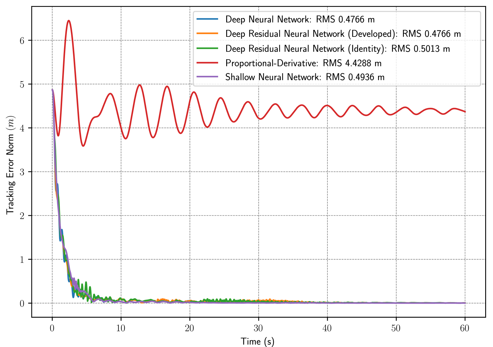
Figure 2: Evolution of tracking error norm $\left\|e\right\|$ over the 60-second simulation period for all controllers.

VII Conclusion

The presented generalized ResNet architecture addresses adaptive control of nonlinear systems with black box uncertainties. Key innovations include pre-activation shortcut connections that improve signal propagation and a zeroth layer block that allows handling different input-output dimensions. The Lyapunov-based adaptation law guarantees semi-global exponential convergence to a neighborhood of the target state.

References

- [1] M. H. Stone, “The generalized Weierstrass approximation theorem,” Math. Mag., vol. 21, no. 4, pp. 167–184, 1948.
- [2] K. Hornik, “Approximation capabilities of multilayer feedforward networks,” Neural Netw., pp. 251–257, 1991.
- [3] P. Kidger and T. Lyons, “Universal approximation with deep narrow networks,” in Conf. Learn. Theory, pp. 2306–2327, 2020.
- [4] A. Kratsios and L. Papon, “Universal approximation theorems for differentiable geometric deep learning,” J. Mach. Learn. Res., 2022.
- [5] F. L. Lewis, “Nonlinear network structures for feedback control,” Asian J. Control, vol. 1, no. 4, pp. 205–228, 1999.
- [6] F. L. Lewis, S. Jagannathan, and A. Yesildirak, Neural network control of robot manipulators and nonlinear systems. Philadelphia, PA: CRC Press, 1998.
- [7] P. Patre, S. Bhasin, Z. D. Wilcox, and W. E. Dixon, “Composite adaptation for neural network-based controllers,” IEEE Trans. Autom. Control, vol. 55, pp. 944–950, 2010.
- [8] Y. LeCun, Y. Bengio, and G. Hinton, “Deep learning,” Nature, vol. 521, no. 436444, 2015.
- [9] I. Goodfellow, Y. Bengio, A. Courville, and Y. Bengio, Deep Learning, vol. 1. MIT press Cambridge, 2016.
- [10] D. Rolnick and M. Tegmark, “The power of deeper networks for expressing natural functions,” in Int. Conf. Learn. Represent., 2018.
- [11] G. Joshi and G. Chowdhary, “Deep model reference adaptive control,” in Proc. IEEE Conf. Decis. Control, pp. 4601–4608, 2019.
- [12] R. Sun, M. Greene, D. Le, Z. Bell, G. Chowdhary, and W. E. Dixon, “Lyapunov-based real-time and iterative adjustment of deep neural networks,” IEEE Control Syst. Lett., vol. 6, pp. 193–198, 2022.
- [13] D. Le, M. Greene, W. Makumi, and W. E. Dixon, “Real-time modular deep neural network-based adaptive control of nonlinear systems,” IEEE Control Syst. Lett., vol. 6, pp. 476–481, 2022.
- [14] O. Patil, D. Le, M. Greene, and W. E. Dixon, “Lyapunov-derived control and adaptive update laws for inner and outer layer weights of a deep neural network,” IEEE Control Syst Lett., vol. 6, pp. 1855–1860, 2022.
- [15] R. Hart, O. Patil, E. Griffis, and W. E. Dixon, “Deep Lyapunov-based physics-informed neural networks (DeLb-PINN) for adaptive control design,” in Proc. IEEE Conf. Decis. Control, pp. 1511–1516, 2023.
- [16] S. Akbari, E. J. Griffis, O. S. Patil, and W. E. Dixon, “Lyapunov-based dropout deep neural network (Lb-DDNN) controller,” arXiv preprint arXiv:2310.19938, 2023.
- [17] M. Ryu and K. Choi, “CNN-based end-to-end adaptive controller with stability guarantees,” arXiv preprint arXiv.2403.03499, 2024.
- [18] D. Le, O. Patil, C. Nino, and W. E. Dixon, “Accelerated gradient approach for deep neural network-based adaptive control of unknown nonlinear systems,” IEEE Trans. on Neural Netw. Learn. Syst., 2024.
- [19] O. S. Patil, E. J. Griffis, W. A. Makumi, and W. E. Dixon, “Composite adaptive Lyapunov-based deep neural network (Lb-DNN) controller,” arXiv preprint arXiv.2311.13056, 2023.
- [20] K. He, X. Zhang, S. Ren, and J. Sun, “Deep residual learning for image recognition,” in Proc. IEEE Conf. Comput. Vis. Pattern Recognit., pp. 770–778, 2016.
- [21] A. Veit, M. Wilber, and S. Belongie, “Residual networks behave like ensembles of relatively shallow networks,” in Proc. 30th Int. Conf. Neural Inf. Process. Syst., pp. 550–558, Curran Assoc. Inc., 2016.
- [22] H. Li, Z. Xu, G. Taylor, C. Studer, and T. Goldstein, “Visualizing the loss landscape of neural nets,” in Proc. 32nd Int. Conf. Neural Inf. Process. Syst., pp. 6391–6401, Curran Assoc. Inc., 2018.
- [23] M. Hardt and T. Ma, “Identity matters in deep learning,” arXiv preprint arXiv.1611.04231, 2017.
- [24] K. Kawaguchi and Y. Bengio, “Depth with nonlinearity creates no bad local minima in ResNets,” Neural Netw., vol. 118, pp. 167–174, 2019.
- [25] K. Nar and S. Sastry, “Residual networks: Lyapunov stability and convex decomposition,” arXiv preprint arXiv:1803.08203, 2018.
- [26] H. Lin and S. Jegelka, “ResNet with one-neuron hidden layers is a universal approximator,” Adv. Neural Inf. Process. Syst., vol. 31, 2018.
- [27] P. Tabuada and B. Gharesifard, “Universal approximation power of deep residual neural networks through the lens of control,” IEEE Trans. Autom. Control, vol. 68, no. 5, pp. 2715–2728, 2023.
- [28] C. Liu, E. Liang, and M. Chen, “Characterizing ResNet’s universal approximation capability,” in Proc. Mach. Learn. Res., vol. 235, pp. 31477–31515, PMLR, 2024.
- [29] K. He, X. Zhang, S. Ren, and J. Sun, “Identity mappings in deep residual networks,” arXiv preprint arXiv.1603.05027, 2016.
- [30] G. Huang, Z. Liu, L. van der Maaten, and K. Q. Weinberger, “Densely connected convolutional networks,” in Proc. IEEE Conf. Comput. Vis. Pattern Recognit., 2017.
- [31] O. S. Patil, D. M. Le, E. Griffis, and W. E. Dixon, “Deep residual neural network (ResNet)-based adaptive control: A Lyapunov-based approach,” in Proc. IEEE Conf. Decis. Control, pp. 3487–3492, 2022.
- [32] P. K. M Krstic, I Kanellakopoulos, Nonlinear and Adaptive Control Design. John Willey, New York, 1995.
- [33] H. K. Khalil, Nonlinear Systems. Prentice Hall, 3 ed., 2002.
- [34] K. Y. Pettersen, “Lyapunov sufficient conditions for uniform semiglobal exponential stability,” Automatica, vol. 78, pp. 97–102, 2017.
- [35] A. Loría and E. Panteley, “Uniform exponential stability of linear time-varying systems: revisited,” Syst. Control Lett., vol. 47, no. 1, pp. 13–24, 2002.